Aerodynamically Balanced Ailerons Commuter Aircraft

Progress in Aerospace Sciences 37 (2001) 497–550

Aerodynamically balanced ailerons for a commuter aircraft

Erkki Soinne1

Royal Institute of Technology and Saab Aerospace, Sweden

Abstract

This review paper describes the state of designing aerodynamically balanced ailerons with a practical application tocommuter aircraft, with Saab 2000 being used as an example. A modern design method is presented based on the

application of CFD computations to determine the aileron aerodynamic data combined with flight mechanicalsimulations to study the impact on airplane rolling maneuvers and aileron dynamics. Dynamic response of ailerondeflection, airplane roll rate and roll acceleration to the applied wheel force is determined by frequency analysis. A

review on the design requirements on ailerons and practical design considerations is presented. The CFD computationsare described in detail with comparisons against wind tunnel experiments and flight tests for validation of themethodology. Description of the flight mechanical simulation system includes the modeling of the aileron control

system. The frequency analysis summarizes the equations of the employed Fourier analysis, spectrum analysis andsystem identification. Numerical results are presented on aileron hinge moment coefficient, airplane rolling momentcoefficient, wheel force in sideslip and rolling maneuvers and gain and phase lag in frequency analysis results to

highlight the key discussion points including the effects of aileron control system and aileron and tab gap sizes. Overall,aerodynamically balanced ailerons, together with a mechanical control system, offer large cost savings on small- andmedium-sized airplanes. r 2001 Elsevier Science Ltd. All rights reserved.

Contents

1. Introduction . . . . . . . . . . . . . . . . . . . . . . . . . . . . . . . . . . . . . . . . . . . . 5012. Two-dimensional trailing edge flow . . . . . . . . . . . . . . . . . . . . . . . . . . . . . . . . 504

2.1. Governing equations . . . . . . . . . . . . . . . . . . . . . . . . . . . . . . . . . . . . . 5042.2. Two-dimensional formulation in ns2d code . . . . . . . . . . . . . . . . . . . . . . . . . 5042.3. Turbulence models . . . . . . . . . . . . . . . . . . . . . . . . . . . . . . . . . . . . . . 505

2.4. Transition model . . . . . . . . . . . . . . . . . . . . . . . . . . . . . . . . . . . . . . . 5062.5. FX 61-163 airfoil . . . . . . . . . . . . . . . . . . . . . . . . . . . . . . . . . . . . . . . 5072.6. FX 66-17AII-182 airfoil . . . . . . . . . . . . . . . . . . . . . . . . . . . . . . . . . . . 509

3. Two-dimensional flow around ailerons . . . . . . . . . . . . . . . . . . . . . . . . . . . . . . 5123.1. NSMB code . . . . . . . . . . . . . . . . . . . . . . . . . . . . . . . . . . . . . . . . . . 512

3.2. MS (1)-0313 airfoil . . . . . . . . . . . . . . . . . . . . . . . . . . . . . . . . . . . . . . 5123.3. DLBA032 airfoil . . . . . . . . . . . . . . . . . . . . . . . . . . . . . . . . . . . . . . . 5143.4. Grid variation and grid convergence . . . . . . . . . . . . . . . . . . . . . . . . . . . . . 515

4. Aerodynamic design of ailerons . . . . . . . . . . . . . . . . . . . . . . . . . . . . . . . . . . 5174.1. Design requirements . . . . . . . . . . . . . . . . . . . . . . . . . . . . . . . . . . . . . 5174.2. Practical design considerations . . . . . . . . . . . . . . . . . . . . . . . . . . . . . . . . 519

4.3. Analysis procedure . . . . . . . . . . . . . . . . . . . . . . . . . . . . . . . . . . . . . . 5234.4. Comparison with flight tests . . . . . . . . . . . . . . . . . . . . . . . . . . . . . . . . . 525

E-mail address: [email protected] (E. Soinne).1Senior Research Scientist

0376-0421/01/$ - see front matter r 2001 Elsevier Science Ltd. All rights reserved.

PII: S 0 3 7 6 - 0 4 2 1 ( 0 1 ) 0 0 0 1 2 - 4

Nomenclature

AcronymsACJ advisory circular-jointADI alternating direction implicitARX auto regression with extra input signalCFD computational fluid dynamicsCFL Courant Friedrichs Levy (number)CG center of gravityCPU central processing unitDFT discrete Fourier transformFAR federal aviation regulationsFAS full approximation schemeFFT fast Fourier transformFPE final prediction errorGflops giga (109) floating point operations per secondJAR joint airworthiness requirementsKCAS knots calibrated air speedKEAS knots equivalent air speedKIAS knots indicated air speedKTAS knots true air speedLU-SGS lower–upper symmetric Gauss–Seidel (implicit solver)MAC mean aerodynamic chordMUSCL monotone upwind schemes for conservation lawsOEI one engine inoperativePFLF power for level flightrms root mean squareSST shear stress transportTVD total variation diminishingVG vortex generator

Notation

A plant matrix; polynomial of ARX modelB control matrix; polynomial of ARX modelc airfoil chord; damping coefficient%cca aileron reference chordcD two-dimensional drag coefficientcf friction coefficientch two-dimensional hinge moment coefficientcL two-dimensional lift coefficientcLp two-dimensional pressure lift coefficientcm:25 two-dimensional pitching moment coefficient referred to 25% chordcLa two-dimensional lift curve slope @cL=@acLd two-dimensional lift coefficient derivative @cL=@da (two-dimensional lift effectiveness)ce1; ce2 turbulence model empirical constantsC system matrixCh control surface hinge moment coefficient, positive when increasing positive deflection (trailing edge down)Cha control surface hinge moment coefficient derivative @Ch=@aChd control surface hinge moment coefficient derivative @Ch=@da

Ch0control surface hinge moment coefficient at zero angle of attack and deflection

C1 rolling moment coefficient based on wing area and span, positive right wing downClp airplane roll damping derivative due to roll rate pCp specific heat in constant pressure; pressure coefficientC *

p critical pressure coefficientCv specific heat in constant volumeds required first cell height

4.5. Effect of tolerances . . . . . . . . . . . . . . . . . . . . . . . . . . . . . . . . . . . . . . 5265. Flight dynamic design of ailerons . . . . . . . . . . . . . . . . . . . . . . . . . . . . . . . . . 530

5.1. Flight mechanical simulations . . . . . . . . . . . . . . . . . . . . . . . . . . . . . . . . 5305.2. Frequency analysis . . . . . . . . . . . . . . . . . . . . . . . . . . . . . . . . . . . . . . 537

6. Summary . . . . . . . . . . . . . . . . . . . . . . . . . . . . . . . . . . . . . . . . . . . . . . 545Acknowledgements . . . . . . . . . . . . . . . . . . . . . . . . . . . . . . . . . . . . . . . . . . 548References . . . . . . . . . . . . . . . . . . . . . . . . . . . . . . . . . . . . . . . . . . . . . . . 548

E. Soinne / Progress in Aerospace Sciences 37 (2001) 497–550498

D system matrixe specific internal energy; unit vector; white noiseE specific total energy; mathematical expectationf damping function in the vicinity of a wallF flux in coordinate direction 1Fa generalized aileron control force; wheel force for roll controlFaer aerodynamic wheel force for roll controlg gravity of earth; gap widthG flux in coordinate direction 2; transfer function#GG transfer function estimate

GðioÞ time continuous frequency function#GGsðioÞ empirical transfer function estimate

GTðeiotÞ sampled frequency functionh specific internal enthalpy; cell length; altitudeH stagnation enthalpy; boundary layer shape parameter; control system local momentHa hinge moment of one aileronHF control system local moment at basic static friction levelH flux tensorI moment of inertia; identity matrixIa aileron moment of inertia around the hinge axisIay product of inertia of the aileron with respect to its hinge line and the x-axisk turbulent kinetic energy; approximation parameter; index for sampling time periods; stiffness coefficientL; M; N aerodynamic moments acting around the body axes x, y and z, respectivelym airplane massM width of lag windowMC design cruise Mach numberMDF demonstrated flight diving Mach numberMMO maximum operating Mach numberMa Mach numbern total number of estimated parametersna parameter defining the order of polynomial Anb parameter defining the order of polynomial Bnk number of delaysng grid level parameternx; ny; nz accelerations in the directions of body axes x; y and z; respectively#nn boundary normal unit vectorN logarithm of the amplification ratio of Tollmien–Schlichting waves; length of sampling data recordp pressure; approximation parameterp; q; r angular rates around the x, y and z axes, respectivelyP production term of turbulencePr Prandtl numberPrT Prandtl number for turbulent flowq heat flux; shift operatorR gas constantRe Reynolds number based on airfoil chordRey Reynolds number based on momentum thicknessReyc critical Reynolds numberRu covariance function of uðtÞRyu covariance function of uðtÞ and yðtÞs length; streamwise coordinatesij strain tensorS area; source term of turbulence; time intervalt timeT temperatureu vector of control inputsu+ dimensionless velocityu; v; w components of the airplane speed projected to the x; y and z axes, respectivelyua; va;wa airplane atmospheric (true) airspeed components projected into the body oriented systemui velocity component in Cartesian coordinate direction xi

Ue velocity at boundary layer external edgeUS estimation of uðtÞ in frequency planeV airplane speedVCLEAN minimum climb speed flaps upVDF demonstrated flight diving speedVFE maximum flaps extended speedVLE maximum speed landing gear extendedVMC minimum control speed

E. Soinne / Progress in Aerospace Sciences 37 (2001) 497–550 499

VMCL minimum control speed in landingVMO maximum speed during normally expected conditions of operation (maximum operating speed)VREF reference speed for landing (landing threshold speed)VS calibrated stalling speed (minimum steady flight speed)VS1 stalling speed with flaps retractedVS1g one-g stall speedV2 takeoff safety speedwðzÞ Hamming window functionW vector of conserved variables; airplane weightWMðtÞ lag windowx state vectorx; y; z Cartesian coordinates; body axes, see Fig. 39xE; yE; zE aircraft position in earth coordinatesxi Cartesian coordinateX ; Y ; Z aerodynamic forces acting in the direction of body axes x; y and z; respectivelyy exact function value; output vectoryn normal distance from wallyþ dimensionless normal distance from wallyðhÞ function value computed with cell size h#yyðt; yÞ estimate of y(t) depending on the model yYS estimation of yðtÞ in frequency planea angle of attackad two-dimensional section lift effectiveness cLd=cLab sideslip angleG circulationda aileron deflectiondaL left aileron deflectiondaR right aileron deflectiondat aileron tab deflectiondf flap deflectiondij Kronecker’s delta’dd control system local deflection rate’ddLIM limit value for control system local deflection ratee dissipation rate of turbulent kinetic energy; prediction errorZ dimensionless spanwise coordinatey boundary layer momentum thickness; elevation angle; parametric modell dimensionless pressure gradient parameterm dynamic viscosity; friction coefficientmt turbulent eddy viscosityn kinematic viscosityr densityse turbulence model constantsk turbulence model constantt time shifttij viscous stress tensortR roll mode time constanttw wall stressf bank angleFu (auto) spectrum of u(t)Fyu spectrum of y(t) and u(t)c azimuth angleond

undamped circular frequency of Dutch rollOij arbitrary quadrilateral cell area

Subscripts

i; j grid indices corresponding to x, y computational coordinates

Superscripts

c convectiven iteration indext turbulentv viscous0 fluctuation� time derivative- time averaged value^ estimate of entity


1. Introduction

A common way of reducing a control surface hingemoment is to use aerodynamic balance or a tab.Aerodynamic balance means having a balance nose

forward of the hinge axis to counteract the hingemoment created by the pressures on the control surfaceaft of the hinge axis. Examples of this are the overhangbalance, the internal (Irving) balance and the horn

balance. Frise aileron is an overhang balance with aspecial nose form to cause flow separation on the lowersurface of a down going aileron nose. A geared tab is

mechanically linked to turn into the opposite directionas the control surface so as to reduce the net hingemoment, see Fig. 1. When the connection between the

control surface and the pilot control wheel is through aspring, permitting a flexible connection, the tab is calleda spring tab. When the spring stiffness is reduced to zero,

so that the direct connection between the control surfaceand the pilot control disappears completely, the pilotsteers directly on the tab which is then called a servo tab.All these configurations can be used for ailerons.

Usually the company tradition and preferences rulewhich solution is chosen.

A combination of aerodynamic balancing and tabs is

generally used on ailerons with a mechanical controlsystem. Aerodynamically balanced ailerons have beenused in general aviation aircraft and up to 150 passenger

transport category airplanes because a mechanicalcontrol system provides large potential in cost savingscompared with a hydraulic system. Usually there is aslot between the control surface and the fixed part of the

airfoil. The flow conditions in the slot are dependent onthe slot and aileron geometry, local angle of attack,Reynolds number and Mach number. This makes the

design of a control surface a demanding task to finda geometry that gives acceptable pilot forces in the entirespeed regime.

Traditionally the design of aerodynamically balancedailerons has largely relied on the practical experience of

aerodynamicists that have been working on the design ofcontrol surfaces. However, after the retirement of theexperienced aerodynamicists, who started their career in

the industry during the 50s, the knowledge is largelygone. Still the potential for cost savings prevails andthere is a need for a better understanding of the flowphenomena.

Reaching the correct Mach and Reynolds numbers isnot easy in a wind tunnel and requires a pressurizedtunnel. Flight tests provide the correct conditions but

are expensive and possible first at a late stage of anaircraft project. CFD is a new method to study theaerodynamics of control surfaces. Compared with

testing it is easy to vary the flow conditions and thegeometry.

The design of ailerons is not, however, only a question

of hinge moments and aerodynamics. The determinationof the wheel force of the pilot additionally requires aknowledge of the mechanical design of the controlsystem and flight mechanics. In a steady maneuver such

as a sideslip a stationary analysis is sufficient. In astationary roll maneuver a quasi-stationary analysis isneeded. An unsteady roll maneuver demands full

dynamic analysis. A prerequisite for this is data on thedynamic stability derivatives which can be determinedwith the help of unsteady aerodynamic theory. The

determination of airplane or aileron response to pilotinput may be studied by frequency analysis usingFourier analysis, spectrum analysis or system identifica-tion. Taking into account the effect of the pilot leads to a

closed-loop system and requires the knowledge ofcontrol theory. The interaction of the pilot and theairplane can also be studied with a flight simulator or

flight test aircraft. A flying simulator aircraft, in whichthe computerized control system may be changed torepresent the prototype airplane, can be used to study

special topics of handling qualities. A prerequisite forailerons with a mechanical control system at mediumor high subsonic speeds is a proper flutter analysis.

In conclusion the development of ailerons involves quitea number of disciplines within aeronautics.

Much of the tedious analysis and pitfalls in the designmay be avoided if experience exists from similar designs.

Hence the cumulated experience from analysis, windtunnel experiments and flight tests, gained during thelast 60 years or so form an invaluable base of knowl-

edge. The general principles of control surface designwere developed already before and during the secondWorld War. The experience gathered in Great Britain

was documented in the classical paper by Morgan andThomas [1]. This paper already describes the problemswith production variability causing variation in control

surface hinge moment. A comprehensive paper onspring tab controls was published by Morgan et al. [2]Fig. 1. Principles of a geared tab and a spring tab.


summarizing the experience gained at RAE. A classicalpaper by Morris [3] treats the implications of icing on

hinge moment coefficient and amount of balance. Theresearch work on lateral control design, conducted atNACA in the United States, was summarized by Toll [4]

after the war.As shown by the literature survey by the author there

are tens of reports on aerodynamic data of controlsurfaces, most of which date back to the 40s. The

classical theory of a thin airfoil with a hinged flap waspresented by Glauert [5] already in the 20s. However,viscous effects strongly dominate the flow around a

control surface and simple analytical theory is notsufficient in general. Semi-empirical methods, takinginto account the effects of boundary layers, are available

in ESDU [6] and DATCOM [7]. These methods arebased on a large number of wind tunnel tests conductedon different geometries such as plain aileron, overhang

balance, Irving balance, horn balance and Frise aileronincluding the effects of gaps and beveled trailing edge.The general trends of the different geometries on aileronhinge moment and lift are summarized by Sears [8] and

Toll [4]. However, the references warn that the trendsmay not be valid for modern airfoil sections differingfrom those employed in the experiments. The only

possibility to obtain data for modern, for example rearloaded sections is to conduct new wind tunnel tests orperform CFD computations.

Published literature on airplane roll control andaileron design is rather limited as shown by theperformed literature survey [9]. Out of the over onehundred references found on aileron aerodynamics only

a small number deals with roll control and ailerondesign. A brief review on aerodynamically balancedcontrol surfaces and ailerons is included in the more

general NACA report [10] by Phillips. Hoerner andBorst [11] commit one chapter on airplane roll control intheir handbook on Fluid Dynamic Lift. There are

descriptions on the development of manual primaryflight controls with aerodynamic balancing on a numberof aircraft shown in Table 1 below. However, only the

references on Pilatus PC-9 are entirely devoted to thedesign of roll control. Masefield [17] gives and interest-ing description on the design of the ailerons on thePilatus PC-9 turboprop trainer. The development of the

ailerons was performed entirely with flight tests bytesting an aileron geometry and then adjusting theconfiguration. To freeze the aerodynamic design over

200 test flights were conducted, the majority of whichconcentrated purely on rolling maneuvers. However onlarger aircraft, due to the high cost of test flights, it is not

possible to base the development of ailerons entirely onflight testing.

The emphasis of this review is twofold. On one hand a

new design methodology is presented based on derivingaileron aerodynamic data using CFD combined with

flight mechanical simulations. On the other hand

practical design experience is reviewed. Both subjectsare studied with the practical application on the 50passenger Saab 2000 commuter aircraft shown in Fig. 2.

Application of Navier–Stokes computations to aileronsis a new field of research with only a few publicationsknown to the author, by Grismer et al. [19], Jiang [20],

Londenberg [21] and Soinne [22]. Due to stringentrequirements on the accuracy of the hinge moment of ahighly balanced aileron, special measures are requiredon grid generation and converged runs. Literature on

aileron dynamics is even more rare with no publishedpapers, known to the author, on civil aircraft.

It is known that in two-dimensional flow, lift is

produced in potential theory only if the stream lines areforced to leave the trailing edge smoothly. This can bedone by prescribing the so-called Kutta condition at the

airfoil trailing edge. On an airfoil with a finite trailingedge angle (e.g. a K!aarm!aan–Trefftz airfoil) a stagnationpoint is formed at the trailing edge. On an airfoil withzero trailing edge angle (e.g. a Joukowsky airfoil) there

is no stagnation point, but the velocities on the upperand lower surfaces of trailing edge are equal. The effectof inertia is included in Euler equations and Kutta

condition is not needed for the computation of lift whenthe airfoil has a trailing edge with a sharp corner. Theeffect of viscosity is introduced with Navier–Stokes

equations and should potentially improve the analysis asviscous phenomena appear in the wake aft of the airfoiltrailing edge. Hence the analysis of the flow conditions

at the trailing edge has a coupling to the creation of lift,a classical question in aerodynamics. The flow condi-tions are especially important on ailerons, because theaileron hinge moment is strongly influenced by the long

moment arm stretching from the trailing edge to thehinge axis.

This review begins with a description of the validation

of the CFD methodology for aileron computations.Because the hinge moment is sensitive to the flowconditions at the airfoil trailing edge, two-dimensional

airfoils were studied first with comparisons against windtunnel experiments in Chapter 2. The next step is thecomputation of a slotted aileron but without aerody-

namic balancing and to compare the results with windtunnel experiments in Chapter 3. Also grid variation

Table 1

Descriptions on roll control development

Airplane Reference Year

Douglas DC-6 [12] 1949

Fokker F28 [13] 1969

Aeritalia G 222 [14] 1972

Dornier 228 [15] 1983

Pilatus PC-9 [16,17] 1988

Aermacchi AMX, MB-326/329 [18] 1990


studies were undertaken in a low speed test case by

refining the grid locally, relaxing the first cell size andincreasing the computational domain size. Grid conver-gence was studied with the help of the basic mesh thatwas created with multiples of 4 cells in every subface

giving three grid levels denoted as coarse, medium andfine mesh levels. A very fine mesh was created separatelyby once more doubling the number of cells in the two

directions. Results at infinitely dense grid level weredetermined by using Richardson’s extrapolation.

Validation of CFD codes is a delicate matter. Every

large code contains errors and discrepancies. Evena theoretically fault-free code has inherent limitationsdue to simplifications in governing equations of the flow

and solution methods. By successfully testing an arbit-rary flow case it is not possible to draw the conclusionthat a program is good for any other flow case. Codeverification, validation, certification and calibration

have drawn increased attention in the past years. Theterminology has been developing but it still seems to besomewhat varying between the authors. Quite a number

of papers has been presented, of which Rizzi and Vos[23] and Roache [24] are two examples. Following thesethe word validation is here used for validation of

calculations by comparing computed results withtrustworthy experimental measurements. The validationprocess is in line with the Guide of AIAA [25].

Comparison of computations with experimental

results usually shows some discrepancy. This may be

due to acknowledged and unacknowledged errors

in modeling and simulation. Examples of the formerare approximations in the modeling of the physicsand round-off errors in the computations. A humanprogramming error is an unacknowledged error. Com-

mon for errors is that they do not arise due to lackof knowledge which, on the contrary, is the casefor uncertainties. For example lack of knowledge

about the complex phenomenon of turbulence resultsin applying simplifications in turbulence modelswith associated uncertainties. Also experiments contain

uncertainties such as the geometrical dimensions of amodel and the measuring accuracy. Therefore the wholeprocess of validation contains some uncertainties.

Aerodynamic design of ailerons is treated in Chapter 4where the design requirements originating from theairworthiness requirements and design specifications aredescribed. The presentation is based on the doctoral

thesis [26] by the author. Practical design considerationsare discussed with issues on maximum wheel force,aileron efficiency and up-floating as well as control

system mechanics. One important issue, namely icing, isnot treated as the ailerons of Saab 2000 have shownproblem-free characteristics. The analysis procedure

from two-dimensional CFD computations to three-dimensional aerodynamic coefficients for the completeaileron is then described. The aerodynamically balanced,type design aileron of Saab 2000 was modeled at two

sections and computations were made at five aileron

Fig. 2. Saab 340 and 2000 commuter aircraft.


deflections in a selected flight test case. The three-dimensional airplane rolling moment and aileron hinge

moment coefficients are compared with the results of adisconnect test flight. The effect of production toleranceswas studied by performing CFD computations on

aileron geometries with a variation on aileron and tabslot gap sizes within the allowable minimum andmaximum values. Also the aileron hinge axis locationwas varied between the typed design and the original

lower positions.A simulation system, based on the flight mechanical

six degree of freedom differential equations, was

employed for flight mechanical simulations on Saab2000 and 340 aircraft. The aircraft models, linkedtogether with the simulation system, contain the airplane

aerodynamics and pertinent aircraft systems such asaileron control system, flaps, engines, landing gear, etc.Simulations were performed in steady heading sideslips

in a flight test case at maximum flaps extended speedVFE: The simulations were performed for the type designaileron geometry and for the aileron without vortexgenerators, based on CFD-derived aerodynamic data.

Roll maneuvers were studied in one low and one highspeed case. In the low speed case, roll control efficiencywas investigated at the reference speed for landing VREF

in landing configuration. In the high speed case, rollcontrol efficiency was investigated in an en-routecondition at airspeeds up to the maximum speed during

normally expected conditions of operation VMO=MMO:The roll maneuvers were studied using the type designgear tab configuration and also a tentative springtab configuration. Also the effect of production toler-

ances was investigated on the aileron slot gap size andthe misrigging of the tab. The results of the flightmechanical simulations are presented in Chapters 5.1.4

and 5.1.5.Frequency analysis was used to study the response

of aileron deflection, airplane roll rate and roll

acceleration to the wheel force applied by the pilot.The frequency response was calculated using Fourieranalysis, spectrum analysis and system identification

employing an ARX model at the lowest value ofminimum control speed in landing when the airplanesare most susceptible to gusts. Computations were alsomade on the effects of flying speed, airplane rolling

moment of inertia, aileron control path stiffness as wellas setting the aileron control system friction anddamping to zero. Simulations on Saab 2000 without

vortex generators were made with pertinent aerody-namic data and by introducing the aileron hingemoment and airplane rolling moment from the CFD

computations. The computed results of the flightdynamic simulations and the frequency analysis arepresented in Chapter 5.2.5. The presentation ends with

concluding remarks and recommendations for futurework in Chapter 6.

2. Two-dimensional trailing edge flow

2.1. Governing equations

The compressible flow Navier–Stokes equations have

the general form, where conservation of mass is written as

@

@trþ

@

@xiðruiÞ ¼ 0 ð1Þ

where r is the density, t the time, and ui the velocitycomponent in Cartesian coordinate direction xi: The

transport equation of momentum is written

@

@tðruiÞ þ

@

@xjðruiuj þ pdijÞ ¼

@tij

@xjð2Þ

where p is the pressure, dij the Kronecker’s delta, and tij

the viscous stress tensor defined for a Newtonian fluid by

tij ¼ m 2sij �2

3

@um

@xmdij

� �ð3Þ

where m is dynamic viscosity and sij is the strain tensor

sij ¼1

2

@ui

@xjþ

@uj

@xi

� �ð4Þ

The conservation of total energy is written as

@

@tr e þ

1

2uiui

� �� þ

@

@xjruj h þ

1

2uiui

� ��

¼@

@xjðuitijÞ �

@qj

@xjð5Þ

where e is the specific internal energy, h the specific

internal enthalpy

h ¼ e þ p=r ð6Þ

and q heat flux. In order to close the system of equationsrelations are needed for pressure, internal energy andtemperature. For a caloric perfect gas the thermodynamicrelations are

e ¼ CvT ð7Þ

p ¼ rRT ð8Þ

where Cv is specific heat in constant volume, R gas

constant and T temperature.

2.2. Two-dimensional formulation in ns2d code

The Saab Navier–Stokes code ns2d [27] solves thetwo-dimensional time-dependent compressible Reynolds

averaged Navier–Stokes equations written in conserva-tive form. The equations are solved in a structuredmulti-block domain. The mean flow equations are

discretized in space using a cell-centered finite volumeapproximation. Central differences are used for theconvective fluxes. For the viscous fluxes the gradients of

velocity and temperature are evaluated at the cellinterfaces using the gradient theorem on auxiliary cells.


The viscous fluxes are then computed in the same way asthe convective fluxes. A blending of adaptive second and

fourth-order artificial dissipation terms are added to thenumerical scheme to damp spurious oscillations andimprove convergence. In the k � e turbulence models,

the diffusive terms are discretized using central differ-ences while for the convective terms a hybrid of upwindand central differencing is used. The discretizationresults in a tridiagonal system of linear algebraic

equations which are solved with an ADI method.The mean flow equations are integrated in time using

an explicit five-step Runge–Kutta scheme. Local time

steps as well as multigrid technique are availablefor convergence acceleration. The multigrid techniqueis based on a full approximation scheme (FAS). The

far-field boundary conditions utilize the one-dimen-sional Riemann invariants combined with a velocitycorrection based on equivalent circulation G: The Airfoil

lift, drag and moment coefficients are determined byintegration of the airfoil surface pressure p and the wallstress tw:

The code has been validated in the BRITE/EURAM

EUROVAL and GARTEUR collaboration projectswith applications such as the Aerospatiale AS239 airfoil(A airfoil), the NLR7301 flapped airfoil and the Airbus

A310 three element airfoil. At Saab the code has beenused for example for the wing flap and horizontal tailcomputations of Saab 2000, for details see Larsson [28].

Integrating the two-dimensional unsteady compressi-ble Reynolds averaged Navier–Stokes equations, writtenin conservative form, over an arbitrary quadrilateral cellOi;j yields, following the nomenclature of ns2d [28]Z Z

Oi;j

@W

@tdS þ

I@Oi;j

HðWÞ #nn ds ¼ 0 ð9Þ

Here the vector of conserved variables contains thefluxes W ¼ r; ru1; ru2; rEf gT; where u1 and u2 are the

mean velocity components in Cartesian coordinatedirections 1 and 2 and E is the specific total energy

E ¼ e þ1

2u2

1 þ u22

� �: ð10Þ

The flux tensor H is composed of convective, viscousand turbulent parts

H ¼ ðF c � Fv � F tÞe1 þ ðGc � Gv � GtÞe2 ð11Þ

in the coordinate directions 1 and 2, respectively. The

convective fluxes are given by

Fc ¼

ru1

ru12 þ p

ru2u1

ru1H

26664

37775; Gc ¼

ru2

ru1u2

ru22 þ p

ru2H

26664

37775 ð12Þ

where H is the stagnation enthalpy

H ¼ E þ p=r: ð13Þ

The viscous and turbulent fluxes are given by

Fv þ F t ¼

0

t11 � ru021

t21 � ru02u01

u1ðt11 � ru021 Þ þ u2ðt12 � ru01u02Þ � q1

2666664

3777775 ð14Þ

Gv þ Gt ¼

0

t12 � ru01u02

t22 � ru022

u1ðt21 � ru02u01Þ þ u2ðt22 � ru022 Þ � q2

2666664

3777775 ð15Þ

An overline denotes time-averaged mean value and anapostrophe a fluctuation. Using Fourier’s law and aclosure approximation for the turbulent part the heat-

flux can be expressed as

qi ¼ �CpmPr

þmT

PrT

� �@T

@xi; i ¼ 1; 2 ð16Þ

where Cp is the specific heat in constant pressure, Pr thePrandtl number, PrT the Prandtl number for turbulent

flow, and mt turbulent eddy viscosity. For a Newtonianfluid the stress tensor tij can be expressed in terms of themean velocity gradients and the dynamic viscosity m as

tij ¼ m@ui

@xjþ

@uj

@xi�

2

3

@um

@xmdij

� �; i; j ¼ 1; 2 ð17Þ

The remaining unknown terms in the system ofequations are the Reynolds stresses �ru0iu

0j : Applying

the Boussinesq eddy viscosity concept the Reynolds

stresses can be expressed as

� ru0iu0j ¼ mT

@ui

@xjþ

@uj

@xi�

2

3

@um

@xmdij

� ��

2

3dijrk

i; j ¼ 1; 2 ð18Þ

where k is turbulent kinetic energy.

Using spatial discretization and numerical integrationin time a stationary solution is sought for the vectorof conserved variables W that satisfies the Navier–

Stokes equations in the entire flow field. Intwo-dimensional flow there are four unknown fluxvariables in every point. The value of turbulent eddyviscosity mt needed in every point is solved through the

turbulence model which introduces up to two additionalunknowns. It is worth while noticing that the elements inthe system matrix are dependent on Mach and Reynolds

numbers.

2.3. Turbulence models

Turbulence models are needed for the closure ofNavier–Stokes equations because direct numerical si-

mulation is not possible in the computation of practicalreal cases due to excessive computing times. In algebraic


turbulence models no differential equations are em-ployed but turbulent eddy viscosity is computed from

the main flow through a set of algebraic equations. Theturbulence models based on two differential equationsare called two-equation models. The k2e turbulence

models employed in this investigation belong to thiscategory. In these models the turbulent kinetic energy kand its dissipation rate e are obtained from theirtransport equations that have a generalized form

@

@tðrkÞ þ

@

@xjðrujkÞ

¼@

@xjmþ

mT

sk

� �@k

@xj

� �þ Pk � re� Sk ð19Þ

@

@tðreÞ þ

@

@xjðrujeÞ

¼@

@xjmþ

mT

se

� �@e@xj

� �þ

ek

ce1 f1Pk � ce2 f2reð Þ � Se;

ð20Þ

where P denotes a production term and S a sourceterm. Factors f are damping functions in the vicinity ofa wall and se; sk; ce1 and ce2 are empirical constants.

Depending on the turbulence model in question someterms may be omitted in the transport equations. Kineticenergy and its dissipation rate can be solved for usingEqs. (19) and (20) and the associated turbulent eddy

viscosity is obtained from the equations applicable forthe turbulence model. In this work one algebraic andthree k2e turbulence models were used. The Baldwin–

Lomax turbulence model [29] is an algebraic model. Oneof the k2e models is the Launder–Sharma turbulencemodel [30]. The two-layer k2e turbulence model is based

on Jones–Launder high Reynolds number turbulencemodel [31] in the outer layer and an adoption Wolfshteinone equation model [32] near the walls. A modified two-layer model is defined by applying an eddy viscosity

limiter, Shear stress transport (SST) in the waysuggested by Menter [33].

2.4. Transition model

Transition is predicted in ns2d code by computing

the laminar boundary layer parameters with Thwaites’method and checking transition due to Tollmien–Schlichting instability waves with the eN-method.Thwaites’ method also gives the separation point

for the laminar boundary layer. The determinationof the transition location is an iterative process in thecode.

In Thwaites’ method algebraic relations are obtainedfrom assumptions of uni-parametric velocity profilesbetween boundary layer momentum thickness y; shape

parameter H and the friction coefficient cf that are theunknowns in the von K!aarm!aan momentum integral

equation

dyds

þ ð2 þ HÞy dUe

Ue ds¼

1

2cf ð21Þ

where s is the streamwise coordinate and Ue the velocityat the boundary layer external edge. By introducing adimensionless pressure gradient parameter

l ¼ry2

mdUe

dsð22Þ

and applying Thwaites’ approximation for the right-

hand side of the rewritten integral equation a first-orderdifferential equation is obtained for the momentumthickness (see Moran [34])

d

dsðy2U6

e Þ ¼ 0:45nU5e ð23Þ

where n is kinematic viscosity.

The velocity of an inviscid flow at stagnation point isgenerally analytic and can be expanded in a power seriesat that point. Substituting a linear approximation for the

velocity into Eq. (23), integrating and assuming that themomentum thickness is finite at the stagnation point anexpression for it is obtained. The momentum thickness

can then be integrated downstream the boundary layerusing Eq. (23). The form parameter is computed asfunction of l using the correlation formulas given by

Cebeci and Bradshaw [35]. If separation of the laminarboundary layer occurs before the transition, it isassumed in the code that transition takes place 2%chord downstream of the separation point.

The transition prediction, based on linear stabilitytheory, assumes that transition will occur when the mostamplified Tollmien–Schlichting waves have grown a

factor eN. Drela and Giles [36] solved the Orr-Sommerfeld equation using Falkner–Skan velocityprofiles for the spatial amplification rates in a range of

shape parameters and unstable frequencies. The loga-rithm of the amplification ratio N is calculated byintegrating the local amplification rate downstream fromthe stagnation point

N ¼Z Rey

Reyc

dN

dReydRey ð24Þ

No amplification will take place for ReyoReyc bysetting dN=dRey ¼ 0: The slope of the maximum

amplification rate dN=dRey is assumed to be only afunction of the local shape factor H using an empiricalrelation and the critical Reynolds number Reyc is also

expressed through an empirical formula (see Drela andGiles [36]). Transition occurs when N reaches somecritical value. Throughout this work the default value

Ncrit=9 has been used.The self-similar Falkner–Skan velocity profiles, on

which the method is based, are not exactly valid for

airfoil boundary layers in general. However, accordingto Dini et al. [37] the shape factor distribution


characteristics of most airfoil flows are smooth enoughand the envelope method of Drela and Giles is

sufficiently accurate before laminar separation.

2.5. FX 61-163 airfoil

The evaluation of the ns2d code was started with asingle component airfoil. The test case should be a well-

known airfoil with experimental data from severalsources. FX 61-163 is a classical laminar airfoil thathas been tested in the laminar flow wind tunnel at the

Technical University of Stuttgart by Althaus [38], at theTechnical University of Delft by Boermans and Selen[39] and at the University of Alberta by Marsden [40].

The quality of the flow in the different tunnels, themeasuring techniques and the accuracy of the windtunnel models are reviewed in Ref. [41] by the author.

The measurements are consistent on lift and dragcoefficient, but on pitching moment the results obtainedin Delft somewhat deviate from those of the other two.This is believed to be a result from the finite trailing edge

thickness and slightly higher thickness ratio of theexperimental model. The conclusion is that the measure-ments are reliable and support each other. The weak

point in the experiments is the model geometry that inthe Delft model was slightly different from the nominalairfoil. The deviation in the Stuttgart model was smaller

but the exact test geometry was not reported.The mesh for the computations was created with an in-

house program at Saab. The created C-mesh has 64 cellsperpendicular and 256 cells parallel to the airfoil surface.

The airfoil trailing edge ends in a single point thus havingzero thickness as shown in the grid in Fig. 3. To guaranteea sufficient resolution in the viscous sublayer the grid was

generated so that the distance from the airfoil contoursatisfies the condition yþp1 for the dimensionless normaldistance from the wall at the first cell centre. This gave a

first cell height in the order of 10�5c.

Four sets of computations were performed in thisstudy:

* transition free at Re=1.5 106 and Ma=0.1, two-layer turbulence model

* transition free at Re=1.5 106 and Ma=0.1, mod-ified turbulence model

* transition fixed at Re=1.0 106 and Ma=0.1, two-

layer turbulence model* transition fixed at Re=2.5 106 and Ma=0.1, two-

layer turbulence model

The transition locations for the smooth airfoil were

taken from the wind tunnel measurements by Althaus[38], because at the time of the computations there wasno transition model available in the code.

The computations were made on a SGI IndigoR4000 workstation with a 32Mb RAM. The two-layerk2e turbulence model was utilized for the computations

and a modification of it with an SST eddy viscositylimiter was employed to study the airfoil stall. Thenumber of workunits1 was selected as 9000 which gave a

run time of 13.5 h with the two-layer model. Conver-gence was controlled by monitoring the rms value of thedensity residual and pressure lift coefficient cLp: Whenusing the modified turbulence model it was not sufficient

to check the density residual when monitoring theconvergence but lift coefficient changed slowly even if nochange was noticed on the density residual. The

iterations were continued until the change in liftcoefficient was less than 1% of its value. This showedto require a number of iterations up to 54,000 work

units.The airfoil polar, computed transition free, is shown

in Fig. 4. As is seen the lift curve slope was approxi-mately 5% higher than the measured reference curve. In

the computed values there was also a shift of roughly0.51 in the zero lift direction. Consequently thecomputed lift coefficient values were around 0.08 higher

than the measured ones in the linear lift range. Thecomputations with transition fixed showed that the liftcurves were lowered due to a thicker boundary layer, see

Figs. 8 and 9 in [41]. However the curves were still abovethe measured ones in the same way as for the smoothairfoil. The two-layer turbulence model did not produce

a complete stall up to the highest angle of attack studied,a=161. The modified turbulence model gave a max-imum lift coefficient of 1.72 at angle of attack a=131.The corresponding measured values are 1.38 at a=111.

Even if there was no boundary layer suction on the windtunnel walls the difference between the computationsand experiments is unexplainably large. The pattern of

stream lines in Fig. 5 shows that in post stall there is alarge flow separation on the airfoil upper surface but onemay question the contraction of the wake.

Fig. 3. A close-up view of the mesh used on FX 61-163 airfoil. 1 Iterations on the fine mesh level.


Fig. 4. Computed and measured [38,39,40] aerodynamic coefficients and transition locations on FX 61-163, smooth airfoil.

Fig. 5. Streamlines for FX 61-163 smooth airfoil, ns2d code, modified two-layer turbulence model.


For the smooth airfoil the computed drag coefficientswere in the laminar bucket 7–20% higher than the

measured ones. The form of the laminar bucket wasreproduced fairly well even at the edges of the bucket.

For smooth airfoil the computed moment coefficient

curve showed a similar form as measured in Stuttgart.The absolute values were somewhat higher,Dcm.25=0.02, which is roughly 20% of the measuredvalue. It is logical that, with computed lift coefficients

exceeding the measured values, the computed momentcoefficients show more negative values than the mea-sured ones, if the deviation is due to the flow conditions

mainly at the airfoil trailing edge. The momentcoefficients for the airfoil with transition fixed atReynolds number 2.5 106 showed only small differ-

ences compared with the transition free case.The performed runs with the Navier–Stokes code ns2d

show that computation of a complete airfoil polar is needed

for insight into the overall performance of a program.Because the lift curve, computed with ns2d, deviated

from the wind tunnel measurements more than expected,calculations with MSES code were made for compar-

ison. MSES is a computer program, developed at MITby Drela [42], for the analysis and design of two-dimensional transonic airfoils and cascades. It uses

Newton method to solve the Euler equations on an intri-nsic streamline grid coupled with an integral boundarylayer method. A detailed description of the theory,

included into the program, is presented by Drela [43].Three sets of calculations were performed at

Re=1.5 106:

* FX 61-163 nominal airfoil.* FX 61-163 with trailing edge thickened to 0.2% of

chord.* FX 61-163 with trailing edge clipped to a thickness of

0.22% of chord.

The three trailing edge geometries are shown in Fig. 6.

The lift and pitching moment curves of the nominal

airfoil, computed with MSES and ns2d, were virtuallythe same in the linear lift range, see Fig. 7. Thethickening of the airfoil trailing edge had only amarginal effect on the lift curve and moment coefficient.

The clipped trailing edge produced considerably less liftand pitching moment.

The chosen FX 61-163 airfoil is a demanding test case.

The computations on the trailing edge modificationsshow that even small changes at a strongly cuspedtrailing edge have a significant effect on the lift and

pitching moment coefficients. This may be a majorexplanation for the differences in the computed andmeasured results as the true trailing edge geometries of

the wind tunnel models are not known.

2.6. FX 66-17AII-182 airfoil

FX 66-17AII-182 airfoil was chosen for furtherstudies because wind tunnel tests, performed in NASAlow-turbulence pressure tunnel at Langley by Somers

[44], were available with a measurement of the actualmodel geometry. The wind tunnel model had a finitethickness trailing edge of 0.08% of the airfoil chord. In

the computations of slotted airfoils by Ashby [45] and deCock and Lindblad [46], the main airfoil blunt trailingedge was modified to end in zero thickness to ease the

meshing and the computations. However, the effect of ageometry modification on the computed results may

Fig. 6. Close-up view of the trailing edge modifications of FX

61-163 airfoil.

Fig. 7. Effect of trailing edge modifications on FX 61-163

airfoil lift and pitching moment curves.


always be questioned. To avoid that kind of discussionthe grid generation was here performed on the exact

wind tunnel model geometry. The airfoil contour isshown in Fig. 8.

The modified C-type mesh was extended 10 chord

lengths away from the airfoil. The four block mesh,contained altogether 30,700 nodes. The number anddistribution of nodes and stretching of cells were basedon the grid variation and grid convergence studies

performed by the author [47]. The geometry of theairfoil blunt trailing edge was accurately modeled byusing 32 cells over the trailing edge thickness, see Fig. 9.

To ensure a sufficient resolution of the boundarylayers the first cell size was based on the requirement ofy+=1 at the cell center. Using the 1/7 power velocity

profile approximation for incompressible flow turbulent

boundary layer over a flat plate (see Schlichting [48]) ananalytic expression was derived for the required first cell

size ds divided by the airfoil chord c

ds

c¼ 2

ffiffiffiffiffiffiffiffiffiffiffiffiffiffiffiffiffiffiffiffiffiffiffiffiffiffiffiffiffiffi0:371=4ðx=cÞ1=5

0:0225Re9=5

sð25Þ

ds=c at the trailing edge (x=c ¼ 1) is plotted in Fig. 10.The incompressible flow assumption gives a slightly

Fig. 8. Contours of FX 66-17AII-182 nominal airfoil and wind

tunnel model.

Fig. 9. Close-up view of the grid at the 0.08% chord thick trailing edge of FX 66-17AII-182 airfoil.

Fig. 10. Maximum first cell size divided by airfoil chord as

function of Reynolds number based on the requirement yþ ¼ 1

at the first cell center at airfoil trailing edge.


conservative estimate for the required cell size, becausethe increase in boundary layer thickness with Mach

number is mainly due to the increase in volume which isassociated with the increase in temperature of the airnear the wall.

A physical explanation can be given on the require-ment of yþ ¼ 1 at the first cell center. In a viscoussublayer, the layer closest to the wall in a turbulentboundary layer, the dimensionless velocity varies line-

arly with the dimensionless normal distance from thewall yþ: This means that for the dimensionless velocityin a viscous sublayer

uþ ¼ yþ ð26Þ

Due to the linear velocity distribution it can be reasonedthat it would be sufficient to have only two cells in this

layer to capture the flow physics. When correct valuesare obtained in these cells it is possible to compute thewall shear stress correctly using the usual two-dimen-

sional approximation

tw ¼ m@ %uu

@yn

� �yn¼0

ð27Þ

and hence also the viscous contribution to airfoil drag.When the viscous effects model properly the drag, they

should also reproduce the boundary layers withsufficient accuracy in other respects such as loss of lift.

The thickness of the viscous sublayer, in which the lawof linearity is valid, is not a precisely defined value.

By general agreement the thickness is chosen as yþ ¼ 5(Schlichting [48], p. 604, White [49], p. 415) and beyondthis, measurements deviate successively more from the

linear law. Taking the value yþ ¼ 5 and covering thisthickness with two cells of equal size gives at the first cellcentre a value yþ ¼ 1:25 which can be rounded off to 1,which is the value based on past experience. The

reasoning above is not valid in separated flows whereuþ goes to infinity and yþ to zero.

Three sets of computations were carried out:

* transition specified according to the wind tunnelmeasurements at Re=1.5 106 and Ma=0.10;

* transition computed with the transition model atRe=1.5 106 and Ma=0.10;

* transition computed with the transition model at

Re=3.0 106 and Ma=0.10.

A special version of the ns2d code was used with thetransition routine implemented. Also the two-layer

turbulence model contained an automatic routine forswitching between the inner and outer models. With a194 MHz SGI Power Challenge processor the computing

time to 20,000 work units was approximately 12 h.Convergence was ensured by monitoring the rms values

Fig. 11. Computed and measured [44] aerodynamic coefficients and transition locations of FX 66-17AII-182 airfoil at Ma=0.1 and

Re=1.5 106. Two-layer turbulence model of ns2d code.


of the time derivatives of the density and turbulentkinetic energy residuals as well as the aerodynamic

coefficients on lift, drag and pitching moment.Complete polars were computed in the three cases

with an example of the results shown in Fig. 11. For

more details see Ref. [50] by the author. The transitionmodel made it possible to make computations withexperimental cases where transition locations where not

measured. At Re=1.5 106 the computed transitionlocations were close to the experimental values. Thecomputed drag polars reproduced the experimental dragvalues fairly well at both Reynolds numbers. The

matching of the computed and measured lift andpitching moment curves was excellent in the linear liftrange. There was no boundary layer suction applied on

the tunnel walls why the experimental values onmaximum lift are somewhat uncertain. Anyhow it isclear that the two-layer turbulence model failed to

predict the airfoil stall.There is also experimental evidence that small

geometrical changes at the airfoil trailing edge, such aswedges and Gurney flaps, have a large effect on airfoil

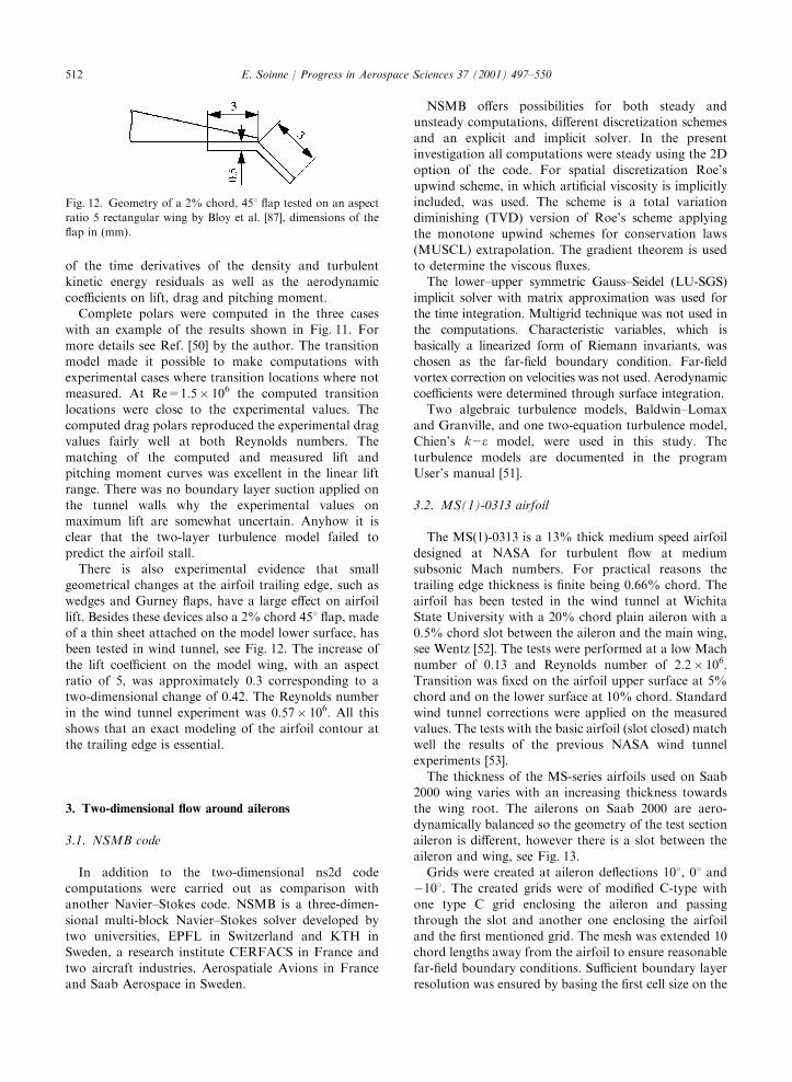
lift. Besides these devices also a 2% chord 451 flap, madeof a thin sheet attached on the model lower surface, hasbeen tested in wind tunnel, see Fig. 12. The increase of

the lift coefficient on the model wing, with an aspectratio of 5, was approximately 0.3 corresponding to atwo-dimensional change of 0.42. The Reynolds number

in the wind tunnel experiment was 0.57 106. All thisshows that an exact modeling of the airfoil contour atthe trailing edge is essential.

3. Two-dimensional flow around ailerons

3.1. NSMB code

In addition to the two-dimensional ns2d codecomputations were carried out as comparison withanother Navier–Stokes code. NSMB is a three-dimen-

sional multi-block Navier–Stokes solver developed bytwo universities, EPFL in Switzerland and KTH inSweden, a research institute CERFACS in France and

two aircraft industries, Aerospatiale Avions in Franceand Saab Aerospace in Sweden.

NSMB offers possibilities for both steady andunsteady computations, different discretization schemes

and an explicit and implicit solver. In the presentinvestigation all computations were steady using the 2Doption of the code. For spatial discretization Roe’s

upwind scheme, in which artificial viscosity is implicitlyincluded, was used. The scheme is a total variationdiminishing (TVD) version of Roe’s scheme applyingthe monotone upwind schemes for conservation laws

(MUSCL) extrapolation. The gradient theorem is usedto determine the viscous fluxes.

The lower–upper symmetric Gauss–Seidel (LU-SGS)

implicit solver with matrix approximation was used forthe time integration. Multigrid technique was not used inthe computations. Characteristic variables, which is

basically a linearized form of Riemann invariants, waschosen as the far-field boundary condition. Far-fieldvortex correction on velocities was not used. Aerodynamic

coefficients were determined through surface integration.Two algebraic turbulence models, Baldwin–Lomax

and Granville, and one two-equation turbulence model,Chien’s k2e model, were used in this study. The

turbulence models are documented in the programUser’s manual [51].

3.2. MS(1)-0313 airfoil

The MS(1)-0313 is a 13% thick medium speed airfoil

designed at NASA for turbulent flow at mediumsubsonic Mach numbers. For practical reasons thetrailing edge thickness is finite being 0.66% chord. The

airfoil has been tested in the wind tunnel at WichitaState University with a 20% chord plain aileron with a0.5% chord slot between the aileron and the main wing,see Wentz [52]. The tests were performed at a low Mach

number of 0.13 and Reynolds number of 2.2 106.Transition was fixed on the airfoil upper surface at 5%chord and on the lower surface at 10% chord. Standard

wind tunnel corrections were applied on the measuredvalues. The tests with the basic airfoil (slot closed) matchwell the results of the previous NASA wind tunnel

experiments [53].The thickness of the MS-series airfoils used on Saab

2000 wing varies with an increasing thickness towards

the wing root. The ailerons on Saab 2000 are aero-dynamically balanced so the geometry of the test sectionaileron is different, however there is a slot between theaileron and wing, see Fig. 13.

Grids were created at aileron deflections 101, 01 and�101. The created grids were of modified C-type withone type C grid enclosing the aileron and passing

through the slot and another one enclosing the airfoiland the first mentioned grid. The mesh was extended 10chord lengths away from the airfoil to ensure reasonable

far-field boundary conditions. Sufficient boundary layerresolution was ensured by basing the first cell size on the

Fig. 12. Geometry of a 2% chord, 451 flap tested on an aspect

ratio 5 rectangular wing by Bloy et al. [87], dimensions of the

flap in (mm).


curve of Fig. 10. The streamwise cell size at the trailingedge and the stretching values were carefully chosen to

ensure sufficient resolution. Again the airfoil trailingedge was modeled accurately avoiding simplifications.Sixty-four cells were chosen over the trailing edge

thickness and across the aileron slot. This gave around62,000 nodes for the two-dimensional ns2d grids and

187,000 for the three-dimensional grids of NSMB.The meshes were visually checked by plotting the

maximum angle deviation, see example in Fig. 14. The

maximum distortion appears in the area where the cellsemanating from the aileron slot meet the cells in theupper and lower boundary layers. This is inevitable witha structured mesh and the distortion is limited to local

small areas. The mesh is so dense in these areas that noanomalies were noticed in the solutions.

The computations were made at a local angle of

attack in the linear lift range representative for theconditions in approach flight with 5% descent gradientat reference speed for landing VREF. In the low speed

case the flight and wind tunnel test conditions are shownin Table 2.

The main alternative for the computations with ns2d

was the two-layer turbulence model. Some computations

Fig. 13. Geometries of Saab 2000 airfoil section at aileron and

two wind tunnel models.

Fig. 14. Maximum angle deviation on the grid of MS(1)-0313 airfoil with a 20% chord plain aileron at aileron deflection da=101.

Table 2

Flight and wind tunnel conditions in the low speed test case

Condition Airfoil Ma Re

Approach flight MS-series 0.19 7.2 106

Wind tunnel test MS(1)-0313 0.13 2.2 106


were also made with Baldwin–Lomax and Launder–Sharma turbulence models for comparisons. ns2d

computations were performed on Cray C90 vectorcomputer having six processors and a theoreticalmaximum performance of 5.7Gflops. Convergence was

monitored on the rms value of the derivatives of thedensity and turbulent kinetic energy residuals as well asthe aerodynamic coefficients of lift, drag and pitchingand hinge moment. Convergence of hinge moment

normally required from 50,000 to 100,000 work unitswhereas the residuals were not a good indicator ofconvergence. Computations with NSMB were per-

formed using the Baldwin–Lomax turbulence modeland k2e turbulence model of Chien. NSMB computa-tions were run on Cray T3E parallel computer using 16

processors. Convergence was monitored on the residualsand the aerodynamic coefficients of lift, drag andpitching moment. The residuals were not a good

indicator on convergence.The numerical results of the computations on MS(1)-

0313 airfoil with the basic set of grids are reported inTable 1 of Ref. [47] by the author. In the low speed test

case at Ma=0.13 and Re=2.2 106 on the MS(1)-0313airfoil the results were practically the same with ns2dand NSMB codes. The computed lift coefficient values

agreed best with the measurements in the case of thenegative aileron deflection of �101 (trailing edge up).The higher the lift coefficient and the more positive the

aileron deflection were, the larger was the differencebetween the computed and measured values. Thesmallest difference in cL was 0.016 and the largest0.138, typically below 0.1. A possible explanation for the

largest difference at positive aileron deflection may bethe fact that k2e turbulence models are known topredict too late a separation on flows with adverse

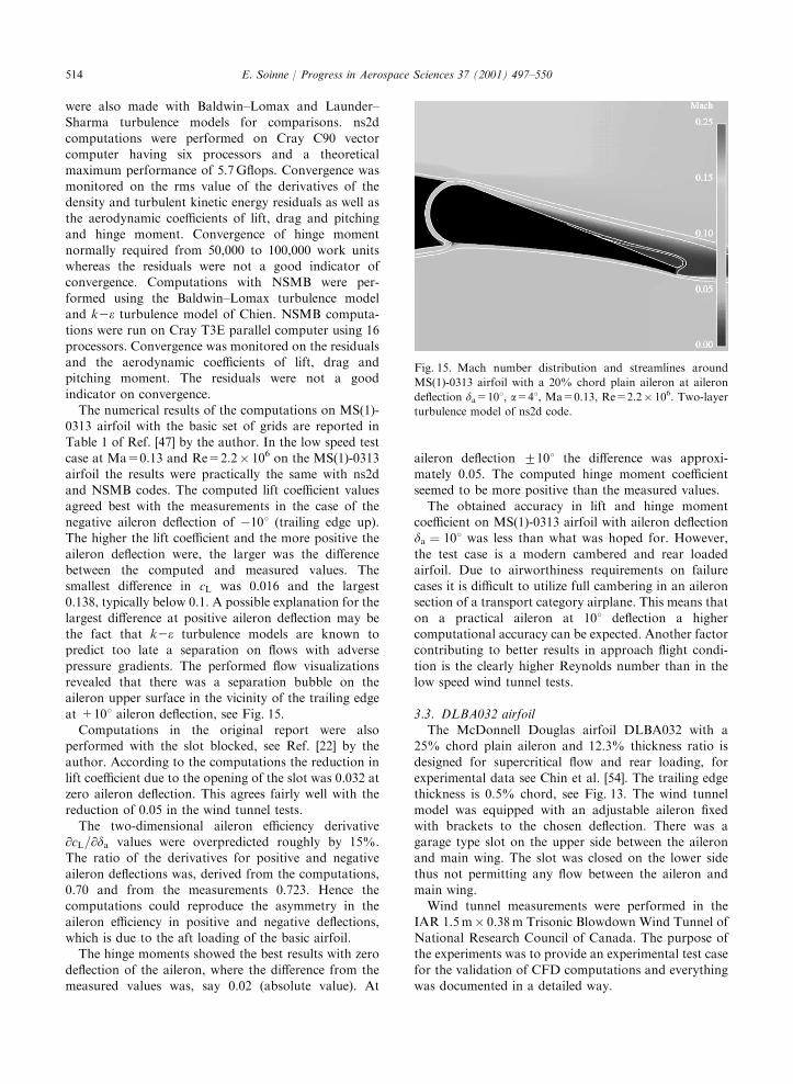
pressure gradients. The performed flow visualizationsrevealed that there was a separation bubble on theaileron upper surface in the vicinity of the trailing edge

at +101 aileron deflection, see Fig. 15.Computations in the original report were also

performed with the slot blocked, see Ref. [22] by the

author. According to the computations the reduction inlift coefficient due to the opening of the slot was 0.032 atzero aileron deflection. This agrees fairly well with thereduction of 0.05 in the wind tunnel tests.

The two-dimensional aileron efficiency derivative@cL=@da values were overpredicted roughly by 15%.The ratio of the derivatives for positive and negative

aileron deflections was, derived from the computations,0.70 and from the measurements 0.723. Hence thecomputations could reproduce the asymmetry in the

aileron efficiency in positive and negative deflections,which is due to the aft loading of the basic airfoil.

The hinge moments showed the best results with zero

deflection of the aileron, where the difference from themeasured values was, say 0.02 (absolute value). At

aileron deflection 7101 the difference was approxi-mately 0.05. The computed hinge moment coefficientseemed to be more positive than the measured values.

The obtained accuracy in lift and hinge momentcoefficient on MS(1)-0313 airfoil with aileron deflectionda ¼ 101 was less than what was hoped for. However,

the test case is a modern cambered and rear loadedairfoil. Due to airworthiness requirements on failurecases it is difficult to utilize full cambering in an aileronsection of a transport category airplane. This means that

on a practical aileron at 101 deflection a highercomputational accuracy can be expected. Another factorcontributing to better results in approach flight condi-

tion is the clearly higher Reynolds number than in thelow speed wind tunnel tests.

3.3. DLBA032 airfoilThe McDonnell Douglas airfoil DLBA032 with a

25% chord plain aileron and 12.3% thickness ratio is

designed for supercritical flow and rear loading, forexperimental data see Chin et al. [54]. The trailing edgethickness is 0.5% chord, see Fig. 13. The wind tunnel

model was equipped with an adjustable aileron fixedwith brackets to the chosen deflection. There was agarage type slot on the upper side between the aileronand main wing. The slot was closed on the lower side

thus not permitting any flow between the aileron andmain wing.

Wind tunnel measurements were performed in the

IAR 1.5m 0.38m Trisonic Blowdown Wind Tunnel ofNational Research Council of Canada. The purpose ofthe experiments was to provide an experimental test case

for the validation of CFD computations and everythingwas documented in a detailed way.

Fig. 15. Mach number distribution and streamlines around

MS(1)-0313 airfoil with a 20% chord plain aileron at aileron

deflection da=101, a=41, Ma=0.13, Re=2.2 106. Two-layer

turbulence model of ns2d code.


The modified C grids were created in the same way asfor the MS(1)-0313 airfoil. The garage type slot, going

halfway through the wind tunnel model between the ail-eron and the main airfoil, was modeled accurately to givethe correct boundary condition at the slot opening. The

number of nodes was 53,000 for the two-dimensional ns2dmesh and 163,000 for the three-dimensional NSMB grid.

For the DLBA032 airfoil the high speed test case waschosen so as to match the local lift at the aileron of Saab

2000 in en-route condition at demonstrated flight divingspeed VDF/MDF. In the high speed case the flight andwind tunnel test conditions are shown in Table 3.

The local aileron angle of attack was selected to matchthe chosen flight case and the aileron deflection was setto +51 so as to represent a typical deflection for aileron

corrective action.Computations were made with ns2d and NSMB codes

using the same turbulence models and computers as for

the MS(1)-0313 airfoil. An extract of the results is shownin Fig. 16. A dashed line shows the value of criticalpressure coefficient C�

p : The pressure coefficient valuesobtained with ns2d code and the two-layer turbulence

model deviate from the measurements not only at theshock wave, but also on the forward part of the airfoilupper and lower surfaces. Results obtained with NSMB

code and Baldwin–Lomax turbulence model matchthe wind tunnel tests clearly better. The suction peak

on the airfoil upper surface in the vicinity of the aileronhinge line is caused by the local upper surface curvatureprotruding into the flow due to the positive aileron

deflection. A contributing factor to the fairly goodresolution of the suction peak was the modeling of thegarage type slot between the aileron and the main wing.The boundary condition at the slot opening is consider-

ably softer than a solid wall condition. The conclusionfrom the computations is that this off design test case is ademanding case for both codes. The angle of attack is so

low that the compression shock wave is so far back thatit interferes with the aileron and the slot.

One turbulence model of each code failed to reach

convergence in the computations with this locallytransonic flow. The two-layer turbulence model ofns2d predicted the shock wave on the aileron upper

surface slightly too far aft. Baldwin–Lomax turbulencemodel of NSMB gave a fairly accurate solution andbetter reproduced the suction peak on aileron uppersurface aft of the slot. A contributing factor to this was

the modeling of the garage type slot between the aileronand main wing to reproduce accurately the wind tunnelmodel geometry. The conclusion from the computations

of the locally transonic flow case is that both codes hadclear difficulties in producing a converged solution in anoff design case giving an impression that the codes are

not in general mature for this type of production runs.

3.4. Grid variation and grid convergence

Because there were no available wind tunnel measure-

ments on a two-dimensional airfoil with a balancedaileron, airfoils with slotted plain ailerons were used atlow and high speeds for the validation of computations.

However, one has to keep in mind that a balancedaileron has a hinge moment coefficient with an order ofmagnitude of 0.01 whereas for a plain type aileron the

order of magnitude is 0.1. This means that one has tocreate the grids so accurately that they are good also fora balanced aileron. Special attention must be paid on thetrailing edge as the fulfillment of the Kutta condition

and the hinge moment coefficient may be sensitive in thisregion due to the long moment arm.

Grid variation studies were undertaken on MS(1)-

0313 airfoil with aileron deflection da ¼ 101 in the lowspeed test case with ns2d code by:

* refining the grid locally in the vicinity of the trailing

edge and slot opening;* relaxing the first cell size;* increasing the computational domain size.

The local streamwise grid refinement from 5 10�4 cto 1 10�4 c in the vicinity of the trailing edge and the

Fig. 16. Pressure coefficient distribution for DLBA032 airfoil

at da=51, a=�0.3291, Ma=0.715, Re=14.8 106, experi-

ments Ref. [54].

Table 3

Flight and wind tunnel conditions in the high speed test case

Condition Airfoil Ma Re

Flight at VDF/MDF MS-series 0.72 10.7 106

Wind tunnel test DLBA032 0.715 14.8 106


slot opening, where separation bubbles appeared,showed no improvement compared with the basic grid.

This was also the case later on with streamwise gridrefinement in the vicinity of the stagnation point onSaab 2000 aileron.

First cell size was relaxed from the conservativelychosen value of the basic grid, corresponding roughly toyþ ¼ 0:5; to more closely fulfill the yþp1 requirement.This relaxation showed no noticeable degradation of the

results.The mesh size was increased from the normal with

external boundary at 10 chord lengths from the airfoil to

20 chord lengths. There was practically no change in theaerodynamic coefficients, which is attributed to theapplied farfield velocity correction based on an equiva-

lent vortex strength.Grid convergence was studied with the help of the

basic mesh that was created with multiples of 4 cells in

every subface giving three grid levels denoted as coarse,medium and fine mesh levels. A very fine mesh wascreated separately by once more doubling the number ofcells in the two directions. The number of nodes on the

very fine grid was approximately 250,000. Becauseobtaining complete grid convergence, i.e. no change ofresults due to grid refinement, is not possible due to

practical limitations on computer resources, the resultsat infinitely dense grid were estimated with Richardson’sextrapolation. The method is originally derived for grids

with a constant cell size but is applied here for grids withvarying cells with the motivation that the cells have thesame form at different mesh levels.

Assume, that when the exact function value y is

approximated by yðhÞ; the function value computed withcell size h; the following holds:

yðhÞ ¼ y þ khp ð28Þ

where k and p are approximation parameters. Byapplying the formula at cell sizes 2h and 4h; the

parameters can be solved for giving the expressions

p ¼logððyð4hÞ � yð2hÞÞ=ðyð2hÞ � yðhÞÞÞ

log2ð29Þ

y ¼ yðhÞ �yð2hÞ � yðhÞ

2p � 1ð30Þ

The function value y at infinite mesh density can now becalculated approximately using the last expression when

the exponent p has first been determined using Eq. (29).The convergence on the very fine mesh was slightly

worse than on the corresponding basic mesh. The

computed results at different grid levels are displayedin Fig. 17 as function of grid level parameter ng: Theparameter is proportional to the number of cells in one

coordinate direction. The results on coarse mesh levelare at 1=ng ¼ 1 and on very fine mesh level at 1=ng ¼

1=8: The scales in the figure have been blown up forpresentation.

On lift coefficient the mesh level had a negligible effect

on the results, but the computed results did not convergetowards the wind tunnel measurements. The fine meshvalue exceeded by 0.138 the wind tunnel test result of

1.03.The hinge moment coefficient converged also quite

well with the fine mesh absolute value being only 0.0002

above the infinite mesh result. However, the computedresults did not converge towards the wind tunnelmeasurements. The fine mesh value fell by 0.051 shortof the wind tunnel test result of �0.29.

The drag coefficient converged towards the experi-mental value with the fine mesh value already beingwithin 3%. The medium and coarse level grids were too

coarse for the determination of the airfoil drag. The gridconvergence on the pitching moment coefficient wasgood but the fine mesh value differed slightly from the

wind tunnel test value.It is obvious that the discrepancy between the

measurements and the fine mesh level values is not dueto changes in grid convergence. The fine mesh results

are so close to the infinite mesh values that the fine

Fig. 17. Grid convergence of aerodynamic coefficients for

MS(1)-0313 airfoil at 101 aileron deflection and a=41,

Ma=0.13, Re=2.2 106. Two-layer turbulence model of

ns2d code.


mesh solution is a good engineering approximation. Thediscrepancies are probably due to the inherent properties

of the turbulence model used.

4. Aerodynamic design of ailerons

4.1. Design requirements

For flight safety reasons airworthiness regulations set

minimum requirements for the handling qualities ofcommercial aircraft. In Europe there are joint require-ments [55] given by the Joint Airworthiness Authorities

JAA and in the United States there are federalregulations [56] published by the Federal AviationAgency FAA. The requirements are continually devel-

oped to increase flight safety. However, when applyingfor the certification of a new airplane it is agreed uponwith the authorities about a certain status of theregulations which the airplane shall meet. In the case

of Saab 2000 the certification basis was frozen to a leveldefined in Ref. [57].

In principle the certification basis stays unchanged

during the development phase of a new airplane.However, there will be a continuous dialog with the

authorities about the interpretation of the regulations.The agreements made are included into the certification

basis as Certification Review Items CRI when workingwith JAA and as Issue Papers when dealing with FAA.JAA also publishes acceptable means of compliance and

interpretations of the regulations in so called ACJs,Advisory Circular - Joint. These additional papersusually specify one way of showing compliance withrequirements that has already been accepted by the

authorities.The regulations however specify only the minimum

acceptable requirements for flying qualities. Optimal

values and gradings are found in American militaryspecifications, MIL Spec [58], Society of AutomotiveEngineers standards [59] or company specifications, an

example of which is Ref. [60]. The background of theMIL Spec is described more in detail by Chalk et al. [61]and MIL-STD-1797A [62]. The standards are based on

research work published for example in NASA reports,see for example Cooper and Harper [63], Holleman et al.[64–66] and Innis et al. [67]. The first reference is theone that defines the well-known Cooper–Harper pilot

rating scale on handling qualities, shown in Fig. 18. Byperforming flight tests and letting different pilots assess acertain parameter, satisfactory and minimum acceptable

Fig. 18. Cooper–Harper handling qualities rating scale [63].


values for the parameter are found. Ratings aboveminimum acceptable do not require (but may warrant)

improvement. Satisfactory values have at least pilotrating 3.5 and minimum acceptable values at least rating6.5 which is just barely certifiable. The MIL Spec [58]

defines flying quality Levels 1–3. At Level 1 the flyingqualities are clearly adequate for the mission flightphase. At Level 2 the flying qualities are adequate toaccomplish the mission flight phase, but some increase in

pilot workload or degradation in mission effectiveness,or both, exists. At Level 3 the airplane can be controlledsafely, but pilot work load is excessive or mission

effectiveness is inadequate, or both. The Cooper–Harperratings 3.5 and 6.5 correspond with the lower limit offlying quality Levels 1 and 2, respectively, of the MIL

Spec (see Chalk et al. [65], p. 18). The lower limit ofLevel 3 corresponds with Cooper–Harper rating 9+.

From the pilots point of view it would be desirable

that the roll control of a commercial airplane has:

* A small break-out force (1–3 lbf) for good controlcentering;

* A linear relationship between control force andaircraft response independent of aircraft speed, inparticular at small control inputs;

* A high steady-state roll rate (30–401/s) over its entireoperational envelope without excessive control forces(max 20–25 lbf);

* A sufficient aileron capacity to safely perform engine-out takeoffs and landings in high cross winds.

However, the pilot would desire optimal character-istics which may differ from minimum acceptablerequirements for flight safety. For example the minimumroll rate specified in the regulations in approach flight is

around 91/s (a 601 roll in 7 s) at reference speed forlanding and around 61/s at minimum control speed inlanding OEI (one engine inoperative, a 601 roll in 11 s).

Designing the ailerons to fulfill the optimal character-istics even in the extreme conditions would produce anairplane with very nice, but uneconomic characteristics.

The certification and optimal design requirements onthe roll control design of a transport category airplanehave been surveyed by the author and are listed in detail

in Ref. [68]. The minimum (certification) requirementsare taken as the most stringent combination of theairworthiness requirements of FAR 25 [56] and JAR 25[55] as an airplane is normally developed for the whole

world market. Requirements with consequences onaileron design are set on lateral control forces, lateralcontrol efficiency, lateral static stability, lateral dynamic

stability and miscellaneous issues such as control systemfailure, control centering and breakout forces. Thedesign requirements are summarized shortly in the

following. For details consult the examples in thefollowing chapters or the survey in Ref. [68].

The certification requirements state at present amaximum control force of 50 lbf for temporary applica-

tion when two hands are available for control and 25 lbfwhen only one hand is available. The values may notexceed prescribed limits neither during takeoff, climb, level

flight, descent and landing nor during a sudden failure ofthe critical engine. In normal operation of the airplane thespeed may vary from minimum control speed VMC tomaximum operating speed VMO/MMO. One hand opera-

tion applies for flight phases where the other hand isneeded for operation of other controls such as powerlever. Hence flare is a case for one hand requirement but

rotation a two hand case. In principle the specifications ofMIL Spec [58] and Boeing [60] conform with therequirements of the certification authorities. For example

the maximum two hand control force of 50 lbf applieseven for fly-by-wire controlled transport aircraft. Require-ments are also set on the linearity of the wheel forces with

control deflection but the requirements are not quantified.Airworthiness regulations set quantified requirements

on lateral control efficiency, to be reached withoutexceeding the maximum allowable wheel forces, in

following cases:

* It should be possible to roll the airplane at takeoff

safety speed V2 one engine inoperative, flaps in takeoffposition and landing gear retracted from a steady 301banked turn through an angle of 601, so as to reverse

the direction of the turn, in not more than 11 s.* To establish the minimum control speed during

landing approach it shall be possible to demonstrate

with the critical engine inoperative and the operatingengines developing maximum take-off power or thrust,that it is possible to roll the airplane through an angleof 201, in the direction necessary to initiate a turn away

from the inoperative engine, in not more than 5 s.* To establish the minimum control speed during

landing approach it shall be possible to demonstrate

with the critical engine inoperative and the thrustnecessary to maintain a gradient of descent of 5%and starting from a condition of straight flight, that it

is possible to roll the airplane through an angle of201, in the direction necessary to initiate a turn awayfrom the inoperative engine, in not more than 3.5 s.

* All engines operating at all powers from flight idle tomaximum continuous power in en-route condition,flaps in en-route position, landing gear retracted,airbrakes in any permitted setting from extended to

retracted it must be possible at airspeed fromminimum value of the scheduled all-engines-operat-ing climb speed VCLEAN to maximum operating

speed VMO/MMO to roll the airplane from a steady301 banked turn through an angle of 601, so as toreverse the direction of turn, in not more than 7 s.

* All engines operating at a power required to give agradient of descent of 5.0% in approach flight


condition, flaps in each landing position, landinggear extended, airbrakes in the maximum permitted

extended setting it must be possible at landingthreshold speed VREF to roll the airplane from asteady 301 banked turn through an angle of 601, so as

to reverse the direction of turn, in not more than 7 s.* To demonstrate that there is adequate roll capability

to assure a prompt recovery from a lateral upsetcondition it should be possible all engines operating at

the power required to maintain level flight at all VMO/MMO, flaps in en-route position, air brakes inpermitted settings from retracted to extended, landing

gear retracted at airspeed from VMO/MMO to a speednot exceeding VDF/MDF during the maneuver to rollthe airplane using lateral control alone from a steady

201 banked turn through an angle of 401, so as toreverse the direction of the turn, in not more than 8 s.

The wheel forces tend to be high in the high speedcases whereas the attainable roll rates tend to be low at

low speed. Ignoring the transient part in these rollmaneuvers the specified values can be transformed intofollowing roll rates as shown in Table 4.

In the same way the specifications of MIL Spec [58]and Boeing [60] set requirements on lateral controlefficiency with increasing roll rates specified at higherspeeds. There are also other requirements on the

airplane roll capability not so easy to apply in designas there are no numerical quantifications. Supplemen-tary recommendations are given by the MIL Spec [58],

Holleman and Gilyard [65] and Holleman and Powers[66] on additional parameters, such as roll control powerand roll mode time constant, as a measure for control

efficiency and control feel.The airworthiness regulations state about lateral static

stability that:

* The static lateral stability, as shown by the tendencyto raise the low wing in a sideslip with the aileron

controls free and for any landing gear and powercondition, may not be negative at any airspeed from1.2VS1 to VMO/MMO.

The requirement does not apply for speeds beyondmaximum flap extended speed VFE or maximum speed

landing gear extended VLE when the flaps or gear, res-pectively, are extended. There is also a requirement thatin straight, steady, sideslips the aileron control move-

ments and forces must be substantially proportional tothe angle of sideslip but the values are not quantified.

Concerning lateral dynamic stability the airworthinessregulations quote that any combined lateral-directional

oscillations (Dutch roll) occurring between stallingspeed and maximum allowable speed appropriate tothe configuration of the airplane must be positively

damped with controls free, and controllable with normaluse of the primary controls without requiring excep-tional pilot skill. However, no numerical values are

specified. Supplementary recommendations are given inthe MIL Spec and literature about flying qualities onlateral directional, roll rate and bank angle oscillations,

spiral stability, sideslip excursions, turn coordinationand pilot induced oscillations.

Miscellaneous certification requirements are given inthe regulations on lateral trimming, stall characteristics

and control system failure that have a connection toaileron design. In preliminary design it is essential totake into account the requirement on control system

failures, treated in paragraphs 25.671 and 25.673 of theairworthiness regulations for transport category air-planes (Refs. [56,55]). It is stated that two-control

airplanes must be able to continue safely in flight andlanding if any one connecting element in the directional-lateral flight control system fails. The wording ‘‘tocontinue safely in flight and landing’’ allows a degrada-

tion of flying qualities and restrictions on flightenvelope. The failure case has a special consequenceon ailerons with a rear loaded airfoil. An aileron tends

to float up when disconnected from the system due to amechanical failure. The up-floating aileron on one sidecreates a rolling moment that must be compensated. In

addition to the mentioned miscellaneous requirementsthere are more detailed recommendations in theliterature on control harmony, control centering and

breakout forces and wheel throw.

4.2. Practical design considerations

4.2.1. Maximum wheel forceSaab 340 was certified in 1984 for a maximum wheel

force of 60 lbf but since then one hand operation in

approach flight with a maximum 25 lbf wheel force hasbeen introduced in Change 13 of JAR 25 [55]. As Saab2000 was originally introduced as a stretched 340 it was

not initially believed that Change 13 would be requiredfor certification. It was assumed that the 60 lbfmaximum wheel force, that had later on been reduced

to 50 lbf, was possible due to grandfather rights.However, this was not accepted by the airworthiness

Table 4

Required roll rates ignoring the transient part of the roll

maneuver

Flight case Speed Roll rate

(deg/s)

Takeoff V2 5.5

Approach VMCL 4.0

Approach VMCL 5.7

En-route VCLEAN to VMO 8.6

Approach VREF 8.6

High speed VMO to VDF 5.0


authorities. The outcome of the discussions with thecertification authorities is summarized in Ref. [69] and

states about one hand cases that:

* The approach/landing flare OEI is a one hand casebut turbulence is not required to be considered.

* Crosswind shall be considered in the one hand case ofapproach/landing flare.

* The transition mode between approach and climb at

OEI go-around is a one hand case.* The following go-around climb is a two hand case.

So in one hand cases the maximum allowable wheelforce is 25 lbf whereas in a two hand case 50 lbf is

permitted.A factor further increasing the wheel forces by 10%

on Saab 2000 is the reduction of control wheel size by

this amount compared with 340. The reason for this wasthe size and placement of the displays for the electronicflight instrument system. The displays were located so

low that the wheel size had to be reduced, otherwise thepilots fists would have shadowed the primary flight datadisplay.

Wheel throw is another factor having impact onwheel forces. On Saab 2000 the maximum control wheelthrow conforms with the value of 801 proposed fora completely mechanical system in the MIL Spec [58].

On MD 80 series aircraft with a mechanical controlsystem the maximum wheel throw is 1201.

The control forces should be something like roll:-

pitch:yaw equal to 1 : 2 : 3–1 : 2 : 4 (SAE Std [59], p. 6,Morgan and Thomas [1], p. 435) but on 2000 the ratiosare about 2 : 1 : 1 due to the powered controls on the

elevator and the rudder. However, this does not seem tobe a problem for the pilots, probably due to therelatively light control forces.

The pilot work load in crosswind landings was

initially high and the reason was not understood. Lateron test flights with Calspan flying simulator showed thatthe pilot work load depended mainly on the wheel

forces. The maximum wheel deflections were around 601if the pilot did not have the strength to turn the wheelfurther with only one hand. After the improvement of

aileron effectiveness with vortex generators and asso-ciated reduction in required wheel deflections theallowable maximum sidewind in landing was increased

from 26 to 40 knots.

4.2.2. Aileron geometryThe wing design of Saab 2000 was based on the

smaller Saab 340 to minimize the cost and program risk.

Both wings have the same planform (Fig. 19) andairfoils, but the wing area of the 2000 is 33% largerand the design cruise Mach number MC has been

increased from 0.5 to 0.66. The aileron designs weresimilar with a geared tab configuration to benefit from

the past experience. During the course of the projectailerons were developed in wind tunnel tests with 10

different geometries. The balance ratio varied in the testsbetween 40% and 50% with a final type design value of45%. As the wing rear spar location was already frozen

when increasing the balance ratio, the aileron hinge lineand trailing edge were moved aft, which shows as anotch in the wing trailing edge. The original wing

sections and the final aileron contours are shown inFig. 20.

The tests were performed in a low speed tunnel with a

1 : 5.7 scaled airplane model. Some high speed tests wereperformed with smaller complete airplane and half-models. One configuration was investigated with differ-ent combinations of vortex generators in a transonic

tunnel. Aileron tabs were not included in any of thewind tunnel models. However, control surface flow issensitive to Reynolds number effects and especially the

low speed wind tunnel test results were not representa-tive of real flight conditions. Control surface flow isoften studied in a pressurized tunnel with a two-

dimensional model so that the correct combination ofReynolds and Mach numbers is reached. It is not alwaysnecessary to reach the full-scale Reynolds number, oftena Reynolds number of 3–4 million is sufficient. Devel-

opment flight tests with a 2000 geometry aileron on

Fig. 19. Saab 2000 airplane.


a Saab 340 were concluded slightly before the first flightof Saab 2000.

The selected aerodynamic balancing is so high that theabsolute value of the hinge moment coefficient derivative@Ch=@da is in the order of 0.05 which is clearly below

the classical rule of thumb limit of 0.075 [3]. Asa consequence production variability on the ailerongeometry introduces variation in the hinge moment.

Production tolerance requirements were set accordingly.The nominal size of the gap between the aileron nose

and the cove varies from 0.33% chord at the aileron rootto 0.48% chord at the aileron tip. A classical rule by

Morgan and Thomas [1] says that when the gap size is lessthan 0.25% chord the gap is effectively sealed and whenthe gap is larger than 0.5% the gap is effectively fully

unsealed. In ESDU ([70,71]) the maximum limit of gapsize has been set at ‘‘about 0.2% chord’’ for a sealed plaincontrol in incompressible two-dimensional flow. In con-

clusion the chosen gap size may be within a sensitive zone.The requirement on control system failures implies

that the rolling moment, created by an up-floating

aileron, must be taken care of. The up-float is even morepronounced with a rear loaded airfoil. Without a specialmechanical connection (bus) between the left- and right-hand side ailerons the rear loading of an airfoil cannot

be utilized on a transport category airplane with ageared tab configuration. On Saab 2000 the rollcompensation is done by the pilots who can disconnect

the left and right ailerons and adjust the other aileron tohave the same deflection. The airplane is then in balancefor steady level flight. However, there must also be

sufficient control authority in the other direction so thatthe remaining aileron can roll the airplane against thefloating one. So the aileron up float may not be too largeto impair the control authority. On Saab 2000 the

consequence has been to deflect the aileron trailing edge

and tab upwards so as to reduce the aileron up float.Another possibility would be to use a downspring as on

Saab 340. The chosen approach has two advantages,namely reduced friction and the ability to handle afailure at any airspeed, as both up-float and tab moment

are subject to the same pressure.The reduced airfoil camber, the slots and the trailing

edge reflexion on the aileron affect the wing lift

distribution because the local lift coefficients aredecreased. Compared with the original airfoil thereduction in local lift coefficient is 0.26 at the aileroninner section and 0.32 at the outer section. This

manifests as a dip over the aileron in the wing liftdistribution as shown in Fig. 21, based on extendedlifting line computations. The effect of the fuselage and

nacelle was ignored in the computations.The induced drag of the wing was determined using

the type design aileron and a wing with the original MS-

series airfoil with no local loss of lift over the aileronspan and no notch in the trailing edge of the wingplanform. The induced drag increase due to the type

design aileron was approximately 2% of the airplanetotal drag in cruise condition.

4.2.3. Aileron effectivenessThe flight tests showed that the down going aileron

was not effective at large deflections. To improve this theaileron hinge line was moved upwards (see Fig. 20) to

improve the flow on the aileron upper surface. Theaileron effectiveness was improved and so was thelinearity of the hinge moment curves, except at large

deflections. The raising of the hinge line also increasedthe aileron up-float significantly and this was anadditional reason for introducing the reflex upwards

on the aileron fixed trailing edge and the trim tab. Lateron the reflex on the tab could be reduced.

Fig. 20. Saab 2000 type design aileron inner and outer sections

and basic airfoils. Fig. 21. Lift distribution of Saab 2000 wing computed with

extended lifting line theory. da=01, df=01, CL=0.36.


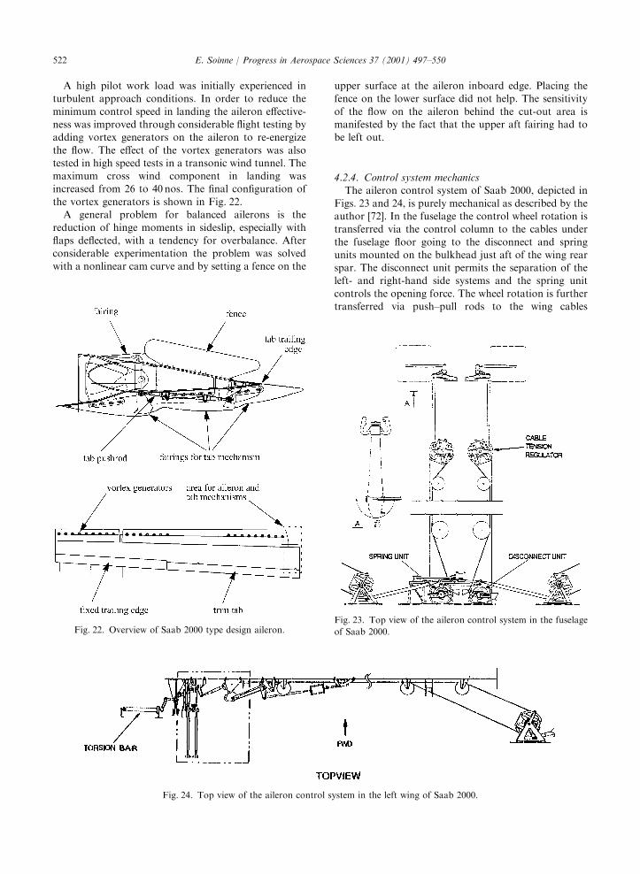
A high pilot work load was initially experienced inturbulent approach conditions. In order to reduce the

minimum control speed in landing the aileron effective-ness was improved through considerable flight testing byadding vortex generators on the aileron to re-energize

the flow. The effect of the vortex generators was alsotested in high speed tests in a transonic wind tunnel. Themaximum cross wind component in landing wasincreased from 26 to 40 nos. The final configuration of

the vortex generators is shown in Fig. 22.A general problem for balanced ailerons is the

reduction of hinge moments in sideslip, especially with

flaps deflected, with a tendency for overbalance. Afterconsiderable experimentation the problem was solvedwith a nonlinear cam curve and by setting a fence on the

upper surface at the aileron inboard edge. Placing thefence on the lower surface did not help. The sensitivity

of the flow on the aileron behind the cut-out area ismanifested by the fact that the upper aft fairing had tobe left out.

4.2.4. Control system mechanicsThe aileron control system of Saab 2000, depicted in

Figs. 23 and 24, is purely mechanical as described by theauthor [72]. In the fuselage the control wheel rotation istransferred via the control column to the cables under

the fuselage floor going to the disconnect and springunits mounted on the bulkhead just aft of the wing rearspar. The disconnect unit permits the separation of theleft- and right-hand side systems and the spring unit

controls the opening force. The wheel rotation is furthertransferred via push–pull rods to the wing cables

Fig. 22. Overview of Saab 2000 type design aileron.

Fig. 24. Top view of the aileron control system in the left wing of Saab 2000.

Fig. 23. Top view of the aileron control system in the fuselage

of Saab 2000.


running along the wing rear spar and terminating at alever assembly at the outboard end of the wing.

The disconnect unit is used by the pilot in a failurecase when there is a jam on one side of the controlsystem to free the other side for the control of the

airplane. When the disconnect is made the ailerons tendto float upwards due to the aft loading of the basicairfoil. To counteract this the aileron fixed trailing edgeand the tab were reflexed upwards and a centering spring

was added on the aileron. A centering spring prevents afloating aileron from oscillating in a failure case.

The tension in the control cables was reduced from

600 to 300 lbf compared with Saab 340 to keep the wheelforces due to friction as low as possible. The air-worthiness regulations do not set requirements on

maximum breakout wheel force but Mil Spec [58] setsa value 6 lbf for a category II land based light or mediumtransport aircraft. So of the maximum 25 lbf one hand

wheel force 6 lbf may be due to friction. On Saab 2000the breakout force is below 4 lbf.

To ensure that full aileron deflections are reachedduring flight under loaded conditions the stops at the

control wheel allow larger deflections on the groundthan the stops at the ailerons. The difference is in theorder of 51 aileron deflection as the cables are relatively

slack in normal operation for low friction. Consequentlythe gearing aileron/wheel deflection diminishes some-what with increasing wheel force.

The centering cams have highly nonlinear character-istics to provide positive wheel forces especially insideslip maneuvers. The centering cams were originallyplaced into the wing but due to space problems they

were moved into the fuselage under the cabin floor (notshown in Fig. 23). There it was possible to enlarge themconsiderably to reduce friction, but virtually no im-

provement was attained in aileron response. This wasprobably due to the slackness of the cables between thecams and the ailerons.

The aileron hinge moments at flap deflection df=151were almost the same as with flaps retracted but atdf=351 the ailerons were considerably heavier. Even-

tually the problem was solved with a variable tabgearing ratio depending on the flap deflection.

4.3. Analysis procedure

In the determination of the aileron aerodynamics theprocedure consists of deriving the local angle of attack

values at two aileron sections chosen for the two-dimensional Navier–Stokes computations, performingthe CFD computations and transforming the two-

dimensional aerodynamic coefficients into three-dimen-sional values for the aileron hinge moment and theairplane rolling moment.

The local angles of attack at the aileron weredetermined with the extended lifting line program LIFLI

(Mai [73]), based on the theory of DeYoung and Harper[74] and Weissinger [75], [76]. LIFLI takes into account

the nonlinearities of the local lift curves, such as airfoilstall, and hence it is possible to combine two-dimen-sional experimental airfoil lift curve data with three-

dimensional computations on wing lift distribution.The fuselage, nacelle and the leading edge extension

between the fuselage and the nacelle were ignored andthe airplane half-wing was divided into five subareas as

shown in Fig. 25. Thus the wing twist distribution couldbe closely approximated with piecewise linear distribu-tions that are assumed in the program. Two-dimensional

airfoil data for MS(1)-0316 and MS(1)-0313 was takenfrom the NASA wind tunnel tests from Refs. [53,77] byMcGhee and Beasley. Interpolations in airfoil thickness

ratio, Reynolds number and Mach number wereperformed where applicable. The two-dimensional sec-tion data over the aileron was determined with CFD

computations from two sections, representative for theinner part with the tab and the outer part with thereflexed aileron trailing edge, see Fig. 20. The sectionswere taken at the aerodynamic centers of each subarea.

LIFLI permits linear interpolation of airfoil lift curvesbetween the end stations of a subarea. The code solvesfor the local lift coefficient which through the local

sectional lift curve yields the local angle of attack.The creation of the computational grids on Saab 2000

aileron sections was based on the experience gained in

the investigations on grid variation and grid conver-gence. The number of nodes on the two-dimensionalgrids for ns2d code ranged from 74,000 on the outersection to 90,000 on the inner section with the tab cavity

modeled. An example of a 15 block grid with the cavitymodeled is depicted in Fig. 31. Plotting of the yþ

distribution in Fig. 26 shows that the value is fairly

constant over the airfoil surface. The value of 1 isexceeded only slightly at the airfoil forward part andlocally in the corners of the slots. Stagnation points in

the vicinity of the airfoil leading edge and on the aileronlower surface are visible through low trough values.

Fig. 25. Modeling of Saab 2000 wing for computations with

LIFLI.


Convergence of the computations was checked by

monitoring the rms values of the derivatives of thedensity and turbulent kinetic energy residuals as well asthe aerodynamic coefficients of lift, drag and pitching

and hinge moment. An example of convergence historiesis shown in Fig. 27. The derivatives of the residuals werenot reliable indicators of convergence because due to

small local time steps in the smallest cells the derivativesreached very high values. However, the absolute changesin the flow, not the derivatives, are of physical interest.The run times on the employed Cray C90 vector

computer having six processors and a theoreticalmaximum performance of 5.7 Gflops were from 40 to100 CPU hours which meant a clock time of 3–7 days.

The longest times were needed at the beginning of thecampaign with a reduction towards the end due toimprovements in the stability criteria of the code per-

mitting the use of higher CFL numbers, see Ref. [78]by the author.

The transformation of the two-dimensional flow hinge

moment coefficient to a three-dimensional value is basedon the handbook method of ESDU. The method isbased on determining the derivatives of the linearizedhinge moment coefficient for a three-dimensional con-

trol surface

Ch ¼ Ch0þ Chaaþ Chdda ð31Þ

where Ch0is the hinge moment coefficient at zero angle

of attack and zero aileron deflection and the two otherterms represent the effects of angle of attack a and

aileron deflection da: A corresponding equation can bewritten for the hinge moment coefficient in two-dimensional flow by formally chancing the capital ‘‘C’’s

to lower case letters. In this work the ratios of thethree-dimensional derivatives to the corresponding

Fig. 27. Convergence history on Saab 2000 aileron inner

section grid. da=101, a=01, Ma=0.298, Re=10.7 106.

Two-layer turbulence model of ns2d code.

Fig. 26. Distribution of yþ in the first cell center on the grid of

Saab 2000 aileron inner section. da=101, a=01, Ma=0.298,

Re=10.7 106.


two-dimensional values were determined and then appliedon the two- and three-dimensional coefficients. The three-

dimensional derivative Chd became generally around 90%of the two-dimensional value whereas the variation in Cha

was somewhat larger. The values of the inner and outer

sections were weighed together in proportion of thereference entities. A correction due to the cut-outs atthe aileron root for the aileron and tab mechanisms andthe hinge at the middle was performed by an approx-

imative integration of the pressure distribution over thebalance nose. The correction term was transformed into athree-dimensional value by proportioning with the

associated reference entities. The amount of correctionhad the same order of magnitude as the basic valueshowing that on a closely balanced aileron the cut-outs

have a considerable effect on the hinge moment.The determination of the airplane rolling moment

coefficient is also based on the handbook method of

ESDU by feeding the CFD-derived section lift effective-ness ad values into the calculations instead of using theempirical graphs. The inner and outer section contribu-tions were weighed together in proportion of the

respective reference areas.

4.4. Comparison with flight tests

The validation cases were selected from the disconnectflight tests. The tests were performed by disconnecting

the control system so that both ailerons could bedeflected in the same direction. The captain deflectedthe control wheel a specified amount and the co-pilot

turned the other control wheel to keep the wings level.The airplane was kept in steady level flight at thespecified flying speed and the aileron hinge moment wasthen measured on one (left) side. The selected test flight

with type design aileron configuration was performed at180 KIAS with zero flap deflection. Because the flyingspeed was kept constant during the measurement the

angle of attack decreased slightly when the ailerons weredeflected downwards and vice versa. This is properlytaken into account in the comparisons with the CFD

computations. The test methodology contains uncer-tainties due to geometrical tolerances, instrumentationand measuring accuracy. By comparison of test results

on left- and right-hand side ailerons it was estimatedthat the total accuracy was around DCh=0–0.005.

The computed three-dimensional hinge momentcoefficients for one aileron are presented together with

flight test results in Fig. 28. The form of the computedcurve matches better the flight test results for the aileronwithout vortex generators. This is as expected because

no account was taken of the VGs in the two-dimensionalmodeling of the CFD computations. Because the wheelforce is given by the difference of the left- and right-hand

side hinge moments, the slope, not the level of the curveis of primary interest.

The complete aileron is very closely balanced with theaerodynamic balance nose and the gearing of the tab.Actually the inner section is overbalanced due to the

geared tab and works against the outer section. Thismeans that the cut-outs at the root and in the middle,shown in Fig. 22, although being small in area, have

a noticeable influence on the aileron hinge moment.Together they gave corrections of the same order ofmagnitude as the basic value. The aileron root part is

difficult to model due to the fence on the upper side andthe fairings on the lower side that modify the pressuredistribution. The gaps in the cut-out area are so large

that they permit a local flow of air through the structure.On the upper side the forward fairing causes a flowseparation on the aileron over the entire width of thecut-out. It is difficult to take into account all these

factors in the three-dimensional hinge moment coeffi-cient. Considering the extremely low hinge momentvalues the case is really demanding and the results are

surprisingly accurate even at �151 and +151 ailerondeflections when flow separations are present.

The airplane rolling moment at 10o aileron deflection,

as calculated from the two-dimensional CFD computa-tions and a transformation applying the method ofESDU, is 3% in excess of the flight test value withvortex generators and 29% in excess without vortex

generators, see Table 5.

Fig. 28. Comparison of hinge moment coefficients on Saab

2000 type design aileron without vortex generators, derived

through CFD computations and flight tests. df=01, V=180

KIAS, trim tab deflection dat=�31 at zero aileron deflection.

Table 5

Airplane rolling moment coefficient Cl at aileron deflections

daL=101 and daR=�101

CFD and transformation Flight test

ESDU, no VGs No VGs With VGs

0.0264 0.0205 0.0256


4.5. Effect of tolerances

One goal of the investigation was to study the effectsof the production tolerances on aileron aerodynamics.The variations of the aileron slot and tab slot gap sizes

as well as the hinge line position of the aileron werepotential factors having an impact on the aileronaerodynamics.

The production tolerances on the tab slot allow a

variation of the constant width gap size g at the tab midsection in an interval of

min g ¼ 0:19% chord

max g ¼ 0:32% chord

with a nominal gap size of 0.23% chord. Except at thetab hinge brackets the actual construction contains a

cavity in front of the tab, see Fig. 29. The cavity was firstmodeled at zero aileron deflection with the nominal gapsize to compare the results with the original constant

width slot. Then the effect of the tab slot was studied bycreating additional six grids with minimum and max-imum gap sizes at aileron deflections da=�101, 01 and101.

On the aileron slot the constant width gap varies

min g ¼ 0:1720:24% chord

max g ¼ 0:4420:64% chord

with the low values referring to the aileron root and thehigh values to the tip. The nominal gap size varies

between 0.34% and 0.49% chord. As the effect of thecavity was globally insignificant the aileron slot gap sizewas studied without modeling the cavity. Altogether 16grids were created at the aileron inner and outer sections

with different gap sizes of the aileron slot at ailerondeflections da=�101, 01 and 101.

The effect of aileron hinge line raise was investigatedby creating three grids at aileron inner section with

nominal gaps and the original low aileron position. Theaileron deflections were again chosen as da=�101, 01and 101.

First the effects of the modeling of the cavity wereinvestigated. Computations on nominal tab slot gap sizewith an without modeling the cavity showed very smalldifferences at zero aileron deflection. On the aerody-

namic coefficients the changes were at maximum twounits on the third significant number. Consequently themodeling of the tab cavity is not of importance when

other effects are studied such as those due to aileron slotgap size and hinge axis position.

However, when the effects of the tab slot area are of

interest simplifications in the local modeling may causediscrepancies. Therefore the tab cavity was modeled forstudying these effects. At 0o aileron deflection the hinge

moment is close to zero and there is very little flowthrough the slot. Consequently the tab slot gap size hasalmost no effect on any of the sectional aerodynamiccoefficients cL; cD; cm:25 and ch: The changes were most

significant on the hinge moment coefficient. At �101 and101 deflections the effects are still small as shown inFig. 30. The influence on the three-dimensional flow

aileron hinge moment coefficient is larger because theaileron intentionally overbalanced inner section worksagainst the outer section with only the moment

difference felt by the aircraft pilot. The effect is howeverstill small compared with the hinge moment curve inFig. 28. The increase of the tab slot gap size tends tosteepen the net hinge moment curve and thus slightly

increases the wheel forces.On lift coefficient the deviations from the nominal

values were less than 0.01 due to the variation of the tab

Fig. 29. Saab 2000 aileron design at a section through the trim/

geared tab, not to scale.

Fig. 30. Effect of tab slot gap size g on two-dimensional hinge

moment coefficient on the inner section of Saab 2000 type

design aileron.


slot gap size. The two-dimensional aileron effectiveness

@cL=@da variation was within 2% from the nominalvalue. Increasing the gap tends to slightly increase thesectional lift coefficient value.

With the ailerons at neutral position no effect wasnoticed on the sectional drag coefficient due to the gapsize variation within the allowable tolerances. The

impact on pitching moment coefficient was negligibleat zero deflection.

An example of the flow in the cavity area is visualized

at aileron deflection 101 in Fig. 32. The flow passes fromthe upper to the lower surface and is considerablyaccelerated when approaching the slot. The primaryvortex in the cavity is slightly compressed to keep the

channel open for the passing flow. Two secondaryvortices are visible in the corners of the cavity.

The second effect studied was that of the aileron slot

gap size. CFD computations were performed withdifferent gap sizes and the effect on the aerodynamiccoefficients at the inner section is depicted in Fig. 33.

Increased gap size causes a noticeable loss of lift. Thetwo-dimensional aileron effectiveness varied at positiveaileron deflections in the tolerance band from �9% to+23% from the nominal value of 0.0319 per degree. At

negative aileron deflections the variation was from �9%

to +20%. The nominal value at negative deflections was0.0327 per degree and consequently the unsymmetry atpositive and negative aileron deflections gives a ratio of

0.98 on aileron effectiveness. Increasing the aileron slot

Fig. 31. Maximum angle deviation on the grid of Saab 2000 aileron inner section at aileron deflection da=101 with tab slot cavity

modeled.


aileron inner section with minimum gap size and raised hinge

axis position at aileron deflection da=101, a=01, Ma=0.298,

Re=10.7 106. Two-layer turbulence model of ns2d code.


gap size diminishes the aileron effectiveness. Note thatthe computed values contain the effect of tab gearing.

On the outer section with the fixed trailing edge theeffectiveness was considerably higher. Contrary to therule of thumb of Morgan and Thomas [1] the slot does

not seem to be ‘‘effectively sealed from the viewpoint oflift’’ below 0.25% chord or ‘‘effectively fully unsealed’’beyond 0.5% chord. On the hinge moment coefficientthere is though a plateau at small gap sizes. A

comparison with wind tunnel tests [8] showed that fora NACA 0009 airfoil with a 30% chord medium noseoverhang control surface and a 35% balance ratio the

hinge moment coefficient did not have a plateau at thelow values of the slot gap size.

On sectional drag coefficient the effect of the gap size

was large when the ailerons were deflected. However,more interesting is the drag variation with ailerons atneutral position, where the change is only �3 and +1

drag counts. Also the impact on pitching momentcoefficient was small at zero deflection amounting from�0.0003 to 0.0005.

The influence of aileron slot gap size on the sectional

hinge moment coefficient was at +101 deflection from0.0091 to �0.0024 corresponding to the minimum andmaximum gap widths, respectively. At �101 deflection,

the corresponding values were �0.0042 and 0.0027. Theincrease of the aileron slot gap size tends to steepen thenet hinge moment curve and thus increase the wheel

forces. This is also true on the outer aileron sectionwhich, due to the fixed trailing edge, is not overbalancedas the inner section. The reason for the hinge momentincrease is that with increased aileron slot gap size the

mass flow through the slot increases. Then the gapcannot sustain the pressure difference between the upperand lower surfaces on the aileron balance nose, see

Fig. 34.The flow patterns at �101 and 01 aileron deflections

were principally the same for the minimum and

maximum gap sizes. With the maximum gap sizethe increased flow through the slot requires more volumeand hence diminishes the vortices in the aileron slot area.

At 101 aileron deflection the flow patterns differ onthe aileron upper surface, see Figs. 35 and 36. On theminimum gap geometry there is a small vortex on topthe aileron balance nose but no flow separation in front

of the tab slot. The maximum gap geometry showsno flow separation on the balance nose (even if the flowis locally retarded with a thickened boundary layer).

In front of the tab slot there is a local region ofseparated flow. Computations with the nominal gap size

3——————————————————————————

Fig. 33. Effect of aileron slot gap size g on two-dimensional

aerodynamic coefficients on the inner section of Saab 2000 type

design aileron.


showed a vortex on the balance nose and abeginning flow separation in front of the tab slot

(Fig. 37).The third effect investigated was that of the hinge axis

position. CFD computations were made with the

original hinge axis position that was 8mm (0.32 in)lower than on the type design aileron. The flow patternswith the low hinge axis position somewhat differ fromthose of the type design aileron. An example is shown in

Figs. 37 and 38 at aileron deflection da=101. With the

nominal gap size the low aileron shows a vortex on thebalance nose and a flow separation in front of the tab

slot. Due to the raised hinge line the flow separation wassuccessfully delayed with an improvement in aileroneffectiveness.

Due to the raise of the hinge line the two-dimensionalaileron effectiveness @cL=@da was increased 12% from0.0286 to 0.0319 per degree at positive deflections. Thechange was 2% from 0.0334 to 0.0327 per degree at

negative deflections. The ratio of sectional aileron

Fig. 34. Pressure coefficient distributions around Saab 2000

type design aileron inner section with two aileron slot gap sizes

at aileron deflection 101, a=01, Re=10.7 106, Ma=0.298.

Two-layer turbulence model of ns2d code.


aileron inner section with maximum aileron slot gap size and

raised hinge axis position at aileron deflection da=101, a=01,


ns2d code.


aileron inner section with minimum aileron slot gap size and



ns2d code.


aileron inner section with nominal aileron slot gap size and



ns2d code.


effectiveness at positive and negative deflections wasimproved from 0.858 to 0.978.

According to the computations the raise of the hingeline gave a drag reduction amounting to 7 drag countswith the ailerons at the neutral position.

The changes due to the aileron hinge line raise on thesectional hinge moment coefficient are noticeable inrelation to the low values of the coefficient. At all ailerondeflections the coefficient became more negative with the

absolute values of the difference varying from 0.0058 to0.0202.

5. Flight dynamic design of ailerons

5.1. Flight mechanical simulations

5.1.1. Governing equations

FORMIC is the simulation system used at Saab forflight mechanical simulations on Saab 340 and Saab2000 aircraft [79]. The aircraft models, linked together

with FORMIC, are based on state-space representationof the flight mechanical six degree of freedom differentialequations, the airplane control system, landing gear,engines and other pertinent systems. Nonlinearities in

the aerodynamic data are fully taken into account. Theflight mechanical modeling has been verified throughcomparison with flight test maneuvers in proof of match

tests, required by the authorities for the airplanesimulator for pilot training.

In the state-space representation the higher-order

flight mechanical differential equations and otherdifferential equations included into the system are

transformed into a set of first-order differential equa-tions that are written in matrix form

’xx ¼ Ax þ Bu ð32Þ

where x is the state vector, ’xx its time derivative and u isthe vector of control inputs, A is the plant matrix and B

the control or input matrix. The output of the system isexpressed in terms of the state and control inputs asfollows:

y ¼ Cx þ Du ð33Þ

where y is the output vector and C and D theappropriate system matrices. Eqs. (32) and (33) aresolved by numerical integration. A version of the

Runge–Kutta third-order integration method, modifiedby Ashour [80] for better performance on stiff equations,is used. The program automatically adjusts the integra-

tion step so that the specified accuracy is reached.The basic flight mechanical equations in the airplane

models are written by treating the earth as a stationary

plane in inertial space. The force balance is written inbody axes (the index b is left out)

X � mg sin y ¼ mð ’uu þ qw � rvÞ ð34Þ

Y þ mg cos y sinf ¼ mð’vvþ ru � pwÞ ð35Þ

Z þ mg cos y cos f ¼ mð ’ww þ pv� quÞ ð36Þ

where X ; Y and Z are the aerodynamic forces acting in

the direction of body axes x; y and z; respectively, asshown in Fig. 39, m is the airplane mass and g thegravity of earth, y the elevation angle and f the bank

angle, u; v and w are the components of the airplanespeed projected to the x; y and z axes, respectively, withdots indicating the corresponding accelerations, p; q andr are angular rates around the x; y and z axes,

respectively.The moment balance is written in the body axes

L ¼ Ix ’pp � Izxð’rr þ pqÞ � ðIy � IzÞqr ð37Þ

M ¼ Iy ’qq � Izxðr2 � p2Þ � ðIz � IxÞrp ð38Þ

N ¼ Iz ’rr � Izxð ’pp � qrÞ � ðIx � IyÞpq ð39Þ

where L; M and N are the aerodynamic moments acting

around the body axes x; y and z; respectively. Themoments of inertia are denoted with I with an obviousconvention for the indices. A dot on the angular rates

indicates time derivative yielding corresponding angularaccelerations.

The Euler angle rates are obtained from kinematics inbody axes

’ff’yy’cc

2664

3775 ¼

1 sinf tan y cos f tan y

0 cos f �sin f

0 sinf sec y cos f sec y

264

375

p

q

r

264375 ð40Þ


aileron inner section with nominal aileron slot gap size and low

hinge axis position at aileron deflection da=101, a=01,


ns2d code.


where f is bank angle, y elevation angle and c azimuthangle.

The relations for the angle of attack a and the sideslip

angle b are also obtained from kinematics

a ¼ atanwa

uað41Þ

b ¼ atan ¼vaffiffiffiffiffiffiffiffiffiffiffiffiffiffiffiffi

u2a þ w2

a

p ð42Þ

where ua; va and wa are the airplane atmospheric (true)airspeed components projected into the body-orientedsystem. The positive directions of a and b are shown

in Fig. 39.The aircraft position in earth coordinates xE; yE and zE

is obtained by applying a general coordinate transforma-

tion from the speed vector ½u v w T in body axes to thespeed vector ½ ’xxE ’yyE ’zzE T: The earth coordinates, denotedwith the index E, are body fixed but parallel with the

earth defined axes in order to simplify coordinatetransformations with respect of acceleration terms. Afourth coordinate system t, based on the airplanetrajectory, is used in the calculations because it simplifies

the trimming (longitudinal and lateral equations).The differential equations (34–39) contain all forces

and moments inclusive those of the airplane controls,

such as ailerons, and are integrated in time using therelations of other pertinent equations. The basic entitiesin the state vector are the airplane position coordinates

xE; yE and zE; speeds u; v and w; Euler angles y; f and cand the rotation rates p; q and r: Because the flight

mechanical equations can be split into the longitudinaland lateral equations the state vectors are also handledseparately. This simplifies trimming the model and

permits three degree of freedom simulations. Thelongitudinal motion basic state vector contains entitiesu; w; q and y and the lateral motion basic state vectorv; p; r; and f:

5.1.2. Aileron control system modeling

The differential equation for the motion of twoailerons without aileron differential and lying in xyplane can be expressed (see Etkin [81])

Ia.dda þ 2Iayðrq þ ’ppÞ ¼ 2Ha þ Fa ð43Þ

where Ia is the aileron moment of inertia around thehinge axis, da the aileron deflection, Iay the product of

inertia of the aileron with respect to its hinge line and thex-axis, Ha the hinge moment of one aileron and Fa thegeneralized aileron control force.

For the purpose of modeling the aileron controlsystem was divided into seven mass points which wereconnected together with weightless springs, see Fig. 40.Because account was taken of the aileron differential,

asymmetric aerodynamics on the left- and right-handsides, etc. one equation was needed for every mass point.This meant that an equation similar to the above

equation was written for every mass point so that therewas a set of seven differential equations. Due to thenonlinearities and backlashes in the control system it

was possible to solve the system of equations onlynumerically.

Fig. 39. Positive directions for flight mechanical entities in the Saab system.


Friction exists at the control wheels, along the control

path at the pulleys and at the ailerons. The frictionfunction uses a basic static friction level, denoted withHF for the corresponding (local) moment, and the(local) deflection rate ’dd as inputs, see Fig. 41. It provides

static friction, starting friction and dynamic frictiondepending on the deflection rate in question. ’ddLIM is alimit value for the deflection rate, established through

engineering judgement, to give a rational dampingcharacteristics in the system. The corner in the frictioncurve, when approaching the limiting values, is rounded

off to ease the numerical integration of the model.Besides the aerodynamic damping of the ailerons, the

small damping in the control path itself due to corrosion

protection grease on the cables and the chain in thecontrol column was also taken into account. Due tonumerical reasons also an internal damping for thecontrol path has been added into the model. This

damping is proportional to the cable elasticity andnumber of pulleys and has been somewhat overesti-mated to provide a stable numerical behavior. Because

the damping is applied on a cable which has a muchhigher resonance frequency than the entire controlsystem, its effect on simulation results is negligible.

The damping functions were linear with respect to thelocal deflection rate ’dd:

There exists a small backlash in the control pathbetween the control wheel and disconnect unit, in the

disconnect unit, in the control path between the

disconnect unit and the aileron and in the autopilotservo. Backlashes in the control system were taken into

account by modeling them as very weak and aileronstops as very stiff springs.

The nonlinear behavior of the centering cams,

disconnect and spring units, aileron differential as wellas nonlinear aerodynamic data were accurately takeninto account in the modeling. The geared tab and springtab were not modeled with a mass point but the tab

deflection was calculated arithmetically as well asthe loads from the tabs (and associated springs) to theaileron. Because trimming directly on a spring tab at

the cams may be inaccurate due to friction in the system,a tentative configuration with one spring tab and onegeared tab with electrical trim function was suggested.

The spring tab with a 42% balance ratio would replacethe existing trim tab at the aileron root part, see Fig. 22.With an unchanged tab area and geometry behindthe hinge line this would move the tab hinge line and the

trailing edge slightly aft. The combined geared tab/trimtab would replace the aileron fixed trailing edge. Themodeling of the type design aileron control system has

been verified by ground response tests.

5.1.3. Aerodynamic data

The aerodynamic data for Saab 2000 and 340 typedesign configurations were taken from the pertinentAerodynamic Design Data Books, based on wind tunnel

experiments and verified through flight tests. Besides theeffect of aileron and tab deflections on the aileron hingemoment coefficient, account is taken of angle of attack

and sideslip, flap angle, power and dynamic effects.Simulations on Saab 2000 were also made on an

aileron configuration without vortex generators. Theaerodynamic data without VGs was based on two-

dimensional Navier–Stokes computations. The two-dimensional flow aerodynamic coefficients on aileronhinge moment and airplane rolling moment were

transformed into three-dimensional values using thehandbook method of ESDU. The difference of the hingemoment coefficient, derived through CFD computation

and ESDU transformation, compared with the flight testresult of the type design aileron with vortex generators is

Fig. 40. Aileron control system model on Saab 2000.

Fig. 41. Modeling of friction.


shown in Fig. 42. This is the effect of leaving out thevortex generators.

On rolling moment the CFD-based computations gave avalue of 3% in excess of the type design airplane rollingmoment. An adjustment was made accordingly on airplane

rolling moment coefficient for simulations when applicable.Aerodynamic data for the simulations of the effects of

aileron slot gap size was based on the type design values.Corrections were made on aileron hinge moment

coefficients, based on the CFD computations, wherethe changes due to the aileron slot size on the innerand outer sections were weighed together. The effect of

the aileron slot gap size on the hinge moment coefficientis shown in Fig. 43. Also the airplane rolling momentvalues due to aileron deflection were adjusted accord-

ingly. The values were derived at aileron deflections

�101 and +101 and extrapolated to cover the maximumpermitted aileron deflections. At 101 aileron deflection

the change due to the maximum aileron slot gap size wasa few percent on the airplane rolling moment coefficientcompared with the nominal gap size.

The effects of the vortex generators and the aileronslot gap size are first order in the sense that the samevalues, derived at Mach number 0.298, are used in thesimulations independent of the airplane speed. Some feel

for the effects of compressibility can be obtained fromthe examples of Fig. 44 where the lift and hinge momentefficiencies are presented for Saab 2000 aileron inner

section. Both effectivenesses first increase and thenslightly decrease with increasing Mach number. Thevariation of lift effectiveness is within 5% whereas of

hinge moment effectiveness it is at maximum 8%.

Fig. 42. Computed difference of hinge moment coefficient DCh

without and with vortex generators as function of aileron

deflection da.

Fig. 43. Effect of aileron slot gap size on aileron hinge moment

coefficient as function of aileron deflection da.

Fig. 44. Computed effect of compressibility on the lift and

hinge moment efficiency on the inner section of Saab 2000 type

design aileron with different aileron slot gap sizes. a=01,

varying Reynolds number.


The high speed values were derived for the flight

conditions (Table 6):The first case represents a test flight case at maximum

allowed speed at the selected altitude and the second one

cruise at maximum altitude and operating speed. TheReynolds numbers were adjusted in the computations toconform with the values above.

5.1.4. Steady heading sideslips

Lateral static stability was investigated in a steadyheading sideslip. Paragraph 25.177 of FAR 25 [56]requires that the static lateral stability, as shown by the

tendency to raise the low wing in a sideslip with aileroncontrols free may not be negative at any airspeed from1.2VS1 to VMO=MMO: The requirement does not applyfor speeds beyond maximum flap extended speed VFE or

maximum speed landing gear extended VLE when theflaps or gear, respectively, are extended. Also in straight,steady sideslips the aileron control movements and

forces must be substantially proportional to the angleof sideslip (within sideslip angles appropriate to theoperation of the airplane).

The flight mechanical simulations were performed forthe type design aileron geometry and for the aileronwithout vortex generators as computed with CFD andtransformed into three-dimensional values using the

ESDU method. The case was investigated with flapsdeflected to df=351 and landing gear down. Theairplane weight was chosen as 19,000 kg (42000 lbs),

center of gravity position at 37% MAC and flying speed165 KCAS with flight idle power, a flight test case atmaximum flaps extended speed VFE with flight test data

available. This is generally not a dimensioning casebecause flight at lower speeds would be more critical asslipstream then has a more adverse effect on the aircraft

rolling moment due to sideslip. The comparison ofcomputations with flight test data in Fig. 45 shows afairly good matching.

Up to sideslip angles of 51 the computations, based on

the hinge moment derived through CFD, are close to theresults of the type design aileron with vortex generators.At large sideslip angles the wheel force gradient, based

on CFD computations, changes sign and even the forcechanges sign meaning that the control wheel would goagainst a stop when released free. The phenomenon was

noticed in early development flight tests on an aileronconfiguration without the fence and the vortex gen-

erators. In other words CFD computations could haveindicated a potential stability problem at an early stage.

It was seen in the simulation results (Fig. 46) thatbetween the configurations with and without vortexgenerators there were only small differences (some tenths

of a degree) in aileron and rudder deflections, bankangle and angle of attack as well as in applied pedalforce. This is consistent with the small 3% adjustment inthe airplane rolling moment coefficient due to CFD-

based computations without the vortex generators. Thechange in wheel force is mainly due to the change in theaileron hinge moment coefficient. In the aerodynamic

data of the type design airplane there is also adependency of aileron hinge moment coefficient onsideslip angle b but this was retained unchanged in both

simulations.Simulations were also carried out for the tentative

spring tab configuration with and without the effect ofvortex generators. It is seen in Fig. 45 that the basic

wheel force curve with vortex generators is more

Fig. 45. Wheel force on Saab 2000 with geared tab and spring

tab as function of sideslip angle b at 165 KCAS, df=351,

landing gear down and flight idle power.

Table 6

Flight cases used for studying compressibility effects

h (ft) V (KTAS) Ma Re

11,000 316 0.497 10.7 106

31,000 364 0.620 9.9 106


nonlinear than the corresponding curve for the typedesign aileron. The reason for this is probablythe nonlinear cam curve that has been tailored for

the type design ailerons. However, the difference in thewheel force for the spring tab configuration withand without VGs is considerably smaller than in the

case of the type design aileron with the geared tab. Thisshows that the self-adjusting spring tab is capable tocompensate for changes in the aerodynamic hingemoment.

5.1.5. Roll maneuversRoll control efficiency was investigated in an ap-

proach condition where ACJ 25.147(e) of JAR 25 [55]requires at reference speed for landing VREF a roll of 601from a steady 301 banked turn so as to reverse the

direction of turn in not more than 7 s. The landing gearshall be extended and the flaps in landing position. Allengines shall be operating at a power required to give a

gradient of descent of 5.0%. The case was investigated ina flight test case at a weight of 21,550 kg (47500 lbs)

corresponding to a speed of VREF=119 KCAS (1.3 VS1).The airplane was trimmed to give a 5% gradient ofdescent.

The flight mechanical simulations were performed forthe type design aileron geometry and for the aileronwithout vortex generators. The hinge moment curve for

the latter configuration was derived through CFD andESDU transformation as well as the rolling momentcoefficient. To get a reasonably coordinated turn theyaw damper/turn coordinator was engaged in the

simulations. An extract of the simulation results inFig. 47, with the control wheel deflections from 101 to701, shows that the omission of VGs gives a reduction of

wheel forces with a tendency for overbalancing. Theabrupt increase of the wheel force in the fastest rollmaneuvers is due to aileron bottoming. The same

simulations were also performed on the spring tabconfiguration. For the same control wheel deflectionsthe times to roll the required 601 are slightly longer thanfor the geared tab, as shown in Fig. 47. This is due to the

elastic coupling to the control command. However,

Fig. 46. Steady heading sideslip simulation on Saab 2000 with geared tab at VFE=165KCAS, df=351, W=19,000kg, CG=37%

MAC, landing gear down and with flight idle power. Solid line type design aileron, dashed line without VGs.


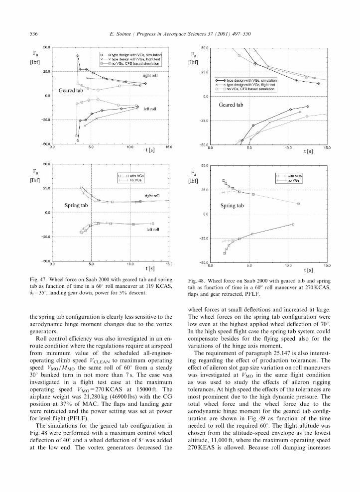
the spring tab configuration is clearly less sensitive to the

aerodynamic hinge moment changes due to the vortexgenerators.

Roll control efficiency was also investigated in an en-

route condition where the regulations require at airspeedfrom minimum value of the scheduled all-engines-operating climb speed VCLEAN to maximum operatingspeed VMO=MMO the same roll of 601 from a steady

301 banked turn in not more than 7 s. The case wasinvestigated in a flight test case at the maximumoperating speed VMO=270 KCAS at 15000 ft. The

airplane weight was 21,280 kg (46900 lbs) with the CGposition at 37% of MAC. The flaps and landing gearwere retracted and the power setting was set at power

for level flight (PFLF).The simulations for the geared tab configuration in

Fig. 48 were performed with a maximum control wheeldeflection of 401 and a wheel deflection of 81 was added

at the low end. The vortex generators decreased the

wheel forces at small deflections and increased at large.The wheel forces on the spring tab configuration were

low even at the highest applied wheel deflection of 701.In the high speed flight case the spring tab system couldcompensate besides for the flying speed also for the

variations of the hinge axis moment.The requirement of paragraph 25.147 is also interest-

ing regarding the effect of production tolerances. Theeffect of aileron slot gap size variation on roll maneuvers

was investigated at VMO in the same flight conditionas was used to study the effects of aileron riggingtolerances. At high speed the effects of the tolerances are

most prominent due to the high dynamic pressure. Thetotal wheel force and the wheel force due to theaerodynamic hinge moment for the geared tab config-

uration are shown in Fig. 49 as function of the timeneeded to roll the required 601. The flight altitude waschosen from the altitude–speed envelope as the lowestaltitude, 11,000 ft, where the maximum operating speed

270 KEAS is allowed. Because roll damping increases


tab as function of time in a 601 roll maneuver at 119 KCAS,

df=351, landing gear down, power for 5% descent.


tab as function of time in a 60o roll maneuver at 270KCAS,

flaps and gear retracted, PFLF.


with decreasing altitude roll rate is expected to decreaseat low altitude. The airplane weight was chosen,almost at the maximum take-off weight, at a value of

22,500 kg (50,000 lbs) with the CG position at 25% ofMAC. The simulation system gave a typical rollingmoment of inertia of 208,000 kgm2, that is 15% belowthe maximum value. Wheel force values due to all

allowed production tolerances, measured in productionaircraft, are shown as comparison. The variation inwheel force due to aileron slot gap size somewhat

exceeds the variation due to the allowed tab riggingtolerances.

The same simulations were performed with the spring

tab configuration with control wheel deflections 81 and10–701 (Fig. 50). The spring tab configuration cancompensate for the variation of the hinge moment dueto the elastic coupling of the aileron much better than

the geared tab.

The investigated cases on one hand of the steadysideslips and low speed roll maneuvers and on the otherhand the high speed roll maneuvers represent the

extreme cases for wheel force. At low speed the wheelforces were low or even reversed sign and at high speedsthe forces were high. The aileron slot gap size had anoticeable effect on the wheel forces with a reduction of

forces with decreasing gap size.

5.2. Frequency analysis

5.2.1. Outline of procedureFrequency analysis was used to study the response of

aileron deflection, airplane roll rate and roll accelerationto the wheel force applied by the pilot. The appliedwheel force was modeled using a chirp signal with

varying frequency. The response of the system in timewas determined with the simulation system FORMIC

Fig. 49. Effect of aileron slot gap size on wheel force Fa and

aerodynamic wheel force Faer on Saab 2000 with geared tab as

function of time to roll 601 at 270KCAS, flaps and gear

retracted, PFLF.

Fig. 50. Effect of aileron slot gap size on wheel force Fa and

aerodynamic wheel force Faer on Saab 2000 with spring tab as

function of time to roll 601 at 270KCAS, flaps and gear

retracted, PFLF.


that produces the output signal at selected discrete timesteps. The frequency response was calculated using

Fourier analysis, spectrum analysis and system identifi-cation employing an ARX model.

Simulink system was used to create a 10 s long signal

with an initial frequency of 0.1Hz and a final frequencyof 2.0Hz. The frequency interval was chosen to coverthe interesting area of human pilot operation in gusty

weather that is known to be around 1 Hz. The amplitudeof the wheel force was chosen as 22.5 lbf (100N). This isjust below the value 25 lbf that is the maximum limit set

by the airworthiness authorities in approach flight withonly one hand operation. By increasing the samplingfrequency until the frequency response results did notchange anymore a frequency of 80Hz was chosen.

The flight case chosen for the studies is approachflight on a 31 glide slope at an altitude of 1000 ft flapsdeflected 351. Because an airplane is most susceptible to

rolling motion disturbances due to turbulence at lowrolling moment of inertia and low speed the lowest valueof reference speed for landing was selected for the

analysis. In ACJ 25.125(a)(2) of JAR 25 [55] it isrequired that the reference landing speed shall not beless than the greater of minimum control speed inlanding VMCL and 1.3 VS where VS is the calibrated

stalling speed. The minimum control speed in landing onSaab 2000 and 340 is limited by roll control and hencealso VREF is limited by aileron effectiveness. The

airplane weights were computed to match the speed1.23 VS1g to cover the requirement of 1.3 VS duringapproach. The factor 1.23 has been used at Saab to

account for the difference2 of the one-g stall speed VS1g

and the calibrated stalling speed VS: The calibratedstalling speed (or minimum steady flight speed) VS takes

into account the momentary reduction of airplanenormal acceleration nz below unity during the stallmaneuver. The selected speeds and correspondingairplane weights are shown in Table 7.

The aerodynamic data for the type design airplaneand the aileron without vortex generators was the sameas in the flight dynamic simulations, see Chapter 5.1.3.

The type design aerodynamic data is based on windtunnel experiments and verified through flight tests. Thedata for the aileron without VGs was either taken from

the official data base or derived with CFD together witha transformation in to three dimension.

Two dynamic derivatives of aileron hinge momentcoefficient are included in the type design data, namely

those with respect of roll rate p and aileron deflectionrate ’dda: The roll rate derivative is coupled with the locala derivative through

@CHa

@pb

2V

� � ¼ Z@CHa

@að44Þ

where b is wing span and Z the dimensionless spanwiselocation 2y=b: The roll rate derivative has low positive

values that tend to increase the rolling.The deflection rate derivative is quite important as it is

known often to supply the main damping of the aileroncontrol system. The value of the derivative on Saab 2000

was identified from flight tests. As there was no flighttest value on 340 a new estimate was computed usingSaab’s unsteady potential flow code Aerel [82], that was

calibrated with the 2000 flight test data. The values forthe derivatives in incompressible flow are shown inTable 8. The value of the damping derivative increased

10% at Mach number 0.6 whereas the roll ratederivative showed no Mach number dependency in theunsteady potential flow computations.

The response of aileron and airplane motion to the

applied sinusoidal wheel force with varying frequencywas determined with FORMIC simulations. The air-plane digital model contains an option to associate

typical moments of inertia to a chosen weight whichgave at the low weights values corresponding to arelatively low level of fuel. The combination of rolling

and sideslipping can create rolling moments that are notpresent when a pilot executes a coordinated roll byapplying the rudder as needed. In the stylized maneuver

the sideslip was suppressed by requiring the yaw angle c;yaw rate r and yaw acceleration ’rr; as well as thelongitudinal and lateral speed components, u and v

respectively, to be constant during the simulation. The

aileron and airplane motions for Saab 2000 type designconfiguration are depicted in Figs. 51 and 52, respec-tively. The applied 22.5 lbf external wheel force produces

a wheel rotation with a decaying amplitude. Also theaileron deflection and aileron aerodynamic hinge mo-ment show damped characteristics. The airplane roll rate

and acceleration time histories resemble the dampedcurves of wheel and aileron deflections. Because the

Table 7

Airplane speeds and weights selected for frequency analysis

VMCL (KIAS) W (lbs)

Saab 340 106 20,000

Saab 2000 111 40,800

Table 8

Dynamic derivative values

@CHa

@’dda %cca

2V

! @CHa

@pb

2V

� �

Saab 2000 �2.80 0.05

Saab 340 �2.04 0.09

2FAR 25 uses VS whereas the requirements of JAR 25 are

based on VS1g:


applied wheel force pulse is not exactly symmetric due to

the increasing frequency the air plane rolls during themaneuver so that the bank angle increases approxi-mately to f=101. The sideslip angle is almost zero

during the entire maneuver.

5.2.2. Fourier analysisThe transfer function GðqÞ of a general linear model

yðtÞ ¼ GðqÞuðtÞ þ vðtÞ ð45Þ

can be estimated with fast Fourier transform (FFT)

when the input and output vectors, uðtÞ and yðtÞ;respectively, are known in discrete form vectors. q isthe shift operator

qyðtkÞ ¼ yðtkþ1Þ ð46Þ

and vðtÞ is a noise term. When the input and outputsignals are known during a finite time interval 0ptpS

estimations on output and input signals

YSðoÞ ¼Z S

0

yðtÞe�iot dt ð47Þ

USðoÞ ¼Z S

0

uðtÞe�iot dt ð48Þ

can be made. Then the empirical transfer function

estimate can be calculated as

#GGSðioÞ ¼YSðoÞUSðoÞ

ð49Þ

When only sampling data is available at time periods

kT ; with k ¼ 1yN; it is natural to use followingapproximations:

YSðoÞ ¼XNk¼1

yðtÞe�iokT ð50Þ

USðoÞ ¼XNk¼1

uðtÞe�iokT ð51Þ

The estimates YSðoÞ and USðoÞ can be computed using

discrete Fourier transform formulas that can be evaluatedusing the recursive formulas of fast Fourier transform.Then N is first adjusted to be a product of 2 by adding

zero values to the output signal. For details of DFT andFFT see R(aade and Westergren [83]. The function calledetfe in MATLAB computes the empirical transfer

function estimate as the ratio of the output Fouriertransform to the input Fourier transform using FFT.

Fig. 51. Time histories of Saab 2000 type design aileron motion in response to an applied wheel force pulse with frequency increasing

from 0.1 to 2.0 Hz.


Comparing the state-space representation of the flight

mechanical differential equations and the equations forthe aileron control system, Eqs. (32) and (33), it is seenthat in transfer function form the equations for the

state-space representation correspond with

GðqÞ ¼ CðqI � AÞ�1B þ D ð52Þ

where I is identity matrix.

5.2.3. Spectrum analysisProvided that the input uðtÞ is independent of noise

vðtÞ the linear system equation (45) implies for theassociated spectra

FyuðoÞ ¼ GðeioÞFuðoÞ: ð53Þ

Consequently the frequency function GðeioÞ can beestimated by estimating the two spectra. The definitionsof the spectra are

FuðoÞ ¼XN

t¼�N

RuðtÞe�iot ð54Þ

FyuðoÞ ¼XN

t¼�N

RyuðtÞe�iot ð55Þ

where the covariance functions RuðtÞ and RyuðtÞ are

RuðtÞ ¼ EuðtÞuðt � tÞ ð56Þ

RyuðtÞ ¼ EyðtÞuðt � tÞ ð57Þ

and E denotes mathematical expectation. The covar-iance functions can be estimated as

#RRuðtÞ ¼1

N

XNt¼1

uðt þ tÞuðtÞ ð58Þ

#RRyuðtÞ ¼1

N

XNt¼1

yðt þ tÞuðtÞ ð59Þ

and the corresponding spectra as

#FFuðoÞ ¼XMt¼�M

#RRuðtÞWMðtÞe�iot ð60Þ

#FFyuðoÞ ¼XMt¼�M

#RRyuðtÞWMðtÞe�iot ð61Þ

WMðtÞ is the so-called lag window

WMðtÞ ¼Z p

�pwðxÞeixt dx ð62Þ

Fig. 52. Time histories of Saab 2000 type design airplane motion in response to an applied wheel force pulse with frequency increasing

from 0.1 to 2.0 Hz.


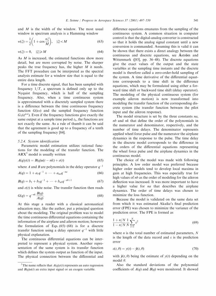
and M is the width of the window. The most usualwindow in spectrum analysis is a Hamming window

wðxÞ ¼1

21 þ cos

pxM

� �; xj joM ð63Þ

wðxÞ ¼ 0; xj jXM ð64Þ

As M is increased, the estimated functions show moredetail, but are more corrupted by noise. The sharperpeaks the true frequency has, the higher M it needs.

The FFT procedure can be interpreted as the spectralanalysis estimate for a window size that is equal to theentire data length.

For a time discrete signal, that has been sampled with

frequency 1=T ; a spectrum is defined only up to theNyquist frequency, which is half of the samplingfrequency. Also, when a time continuous system

is approximated with a discretely sampled system thereis a difference between the time continuous frequencyfunction GðioÞ and the sampled frequency function

GTðeiotÞ: Even if the frequency functions give exactly thesame output at a sample time period tk; the functions arenot exactly the same. As a rule of thumb it can be said

that the agreement is good up to a frequency of a tenthof the sampling frequency [84].

5.2.4. System identificationParametric model estimation utilizes rational func-

tions for the modeling of the transfer function. The

ARX3 model is usually written

AðqÞyðtÞ ¼ BðqÞuðt � nkÞ þ eðtÞ ð65Þ

where A and B are polynomials in the delay operator q�1

AðqÞ ¼ 1 þ a1q�1 þ?þ anaq�na ð66Þ

BðqÞ ¼ b1 þ b2q�1 þ?þ bnbq�nbþ1 ð67Þ

and eðtÞ is white noise. The transfer function then reads

GðqÞ ¼ q�nk BðqÞAðqÞ

: ð68Þ

At this stage a reader with a classical aeronauticaleducation may, like the author, put a principal questionabout the modeling. The original problem was to model

the time continuous differential equations containing theinformation of the airplane and aileron motion; howeverthe formulation of Eqs. (65)–(68) is for a discrete

transfer function using a delay operator q�1 with littlephysical explanation.

The continuous differential equations can be inter-

preted to represent a physical system. Another repre-sentation of the same system is its transfer functionwhich defines the system output as function of the input.

The physical connection between the differential and

difference equations emanates from the sampling of thecontinuous system. A common situation in computer

control is that the digital-analog converter is constructedso that it holds the analog signal constant until a newconversion is commanded. Assuming this is valid it can

be shown that there exists a direct analogy between thecontinuous and discrete equations, see (AAstr .oom andWittenmark ([85], pp. 36–48). The discrete equationsgive the exact values of the output and the state

variables at the sampling time instants and the discretemodel is therefore called a zero-order-hold sampling ofthe system. A time derivative of the differential equat-

ions corresponds to a time shift in the differenceequations, which may be formulated using either a for-ward time shift or backward time shift (delay operator).

The modeling of the physical continuous system (forexample aileron motion) is now transformed intomodeling the transfer function of the corresponding dis-

crete system (the transfer function between the pilotinput and the aileron response).

The model structure is set by the three constants na;nb and nk that define the order of the polynomials in

the numerator and denominator, respectively, and thenumber of time delays. The denominator representsapplied wheel force pulse and the numerator the airplane

dynamics in the response to the pulse. The time delayin the discrete model corresponds to the difference inthe orders of the differential equations representing

the wheel force pulse and the airplane dynamics in thecontinuous model.

The choice of the model was made with followingprinciples. A low order model was preferred because

higher order models tend to develop local maxima ingain at high frequencies. This was especially true forhigh values of nb as the order of modeling for the aileron

deflection was increased. It was more important to havea higher value for na that describes the airplanedynamics. The order of time delays was chosen to

minimize the loss function.Because the model is validated on the same data set

from which it was estimated Akaike’s final prediction

error (FPE) was chosen to minimize the variance of theprediction error. The FPE is formed as

1 þ n=N

1 � n=N

1

N

XNt¼1

e2 ð69Þ

where n is the total number of estimated parameters, Nis the length of the data record and e is the predictionerror

eðt; yÞ ¼ yðtÞ � #yyðt; yÞ ð70Þ

with #yyðt; yÞ being the estimate of yðtÞ depending on themodel y:

Also the standard deviations of the polynomialcoefficients of AðqÞ and BðqÞ were monitored. It showed

3The name reflects that AðqÞyðtÞ represents an auto regression

and BðqÞuðtÞ an extra input signal or an exogen variable.


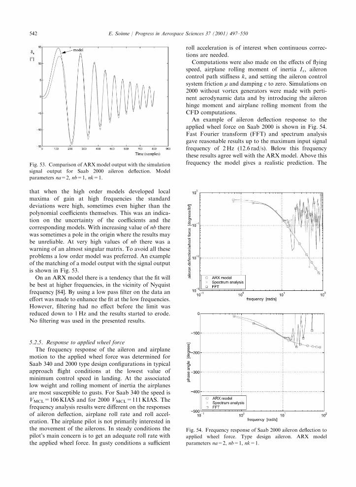
that when the high order models developed localmaxima of gain at high frequencies the standard

deviations were high, sometimes even higher than thepolynomial coefficients themselves. This was an indica-tion on the uncertainty of the coefficients and the

corresponding models. With increasing value of nb therewas sometimes a pole in the origin where the results maybe unreliable. At very high values of nb there was a

warning of an almost singular matrix. To avoid all theseproblems a low order model was preferred. An exampleof the matching of a model output with the signal outputis shown in Fig. 53.

On an ARX model there is a tendency that the fit willbe best at higher frequencies, in the vicinity of Nyquistfrequency [84]. By using a low pass filter on the data an

effort was made to enhance the fit at the low frequencies.However, filtering had no effect before the limit wasreduced down to 1Hz and the results started to erode.

No filtering was used in the presented results.

5.2.5. Response to applied wheel forceThe frequency response of the aileron and airplane

motion to the applied wheel force was determined for

Saab 340 and 2000 type design configurations in typicalapproach flight conditions at the lowest value ofminimum control speed in landing. At the associatedlow weight and rolling moment of inertia the airplanes

are most susceptible to gusts. For Saab 340 the speed isVMCL=106KIAS and for 2000 VMCL=111 KIAS. Thefrequency analysis results were different on the responses

of aileron deflection, airplane roll rate and roll accel-eration. The airplane pilot is not primarily interested inthe movement of the ailerons. In steady conditions the

pilot’s main concern is to get an adequate roll rate withthe applied wheel force. In gusty conditions a sufficient

roll acceleration is of interest when continuous correc-tions are needed.

Computations were also made on the effects of flyingspeed, airplane rolling moment of inertia Ix; aileroncontrol path stiffness k; and setting the aileron control

system friction m and damping c to zero. Simulations on2000 without vortex generators were made with perti-nent aerodynamic data and by introducing the aileronhinge moment and airplane rolling moment from the

CFD computations.An example of aileron deflection response to the

applied wheel force on Saab 2000 is shown in Fig. 54.

Fast Fourier transform (FFT) and spectrum analysisgave reasonable results up to the maximum input signalfrequency of 2 Hz (12.6 rad/s). Below this frequency

these results agree well with the ARX model. Above thisfrequency the model gives a realistic prediction. TheFig. 53. Comparison of ARX model output with the simulation

signal output for Saab 2000 aileron deflection. Model

parameters na=2, nb=1, nk=1.

Fig. 54. Frequency response of Saab 2000 aileron deflection to

applied wheel force. Type design aileron. ARX model

parameters na=2, nb=1, nk=1.


responses on airplane roll rate and roll acceleration

showed the same type of agreement.The frequency analysis results on aileron deflection

response to the applied wheel force pulse, obtained with

the ARX model in the approach flight case, aresummarized in Fig. 55. The amplitude gain of ailerondeflection on Saab 2000 increases with decreasingfrequency. Below a cross-over frequency of 0.4Hz the

gain on 2000 is higher than on Saab 340 and lowerabove. Saab 340 shows a weak resonance peak at 0.6Hz.Ignoring friction and damping (m ¼ c ¼ 0) on the

control system of the 2000 type design aileron yields amarked increase in the gain of the aileron deflection witha peak at 0.6 Hz. The effect of suppressing the friction

and damping (m ¼ c ¼ 0) in the control system is muchlarger on 340 with a pronounced peak in gain at 0.9Hz.This is partly due to the inherently higher control systemfriction on 340 due to a higher tension of the control

cables. The main reason is however the remaining

aerodynamic damping. Due to the airplane larger size(and the small difference in VMCL) the aerodynamic

damping moment on aileron hinge axis is a factor 2.6higher on 2000. On aileron deflection the frequencyresponse of Saab 2000 aileron without vortex genera-

tors, based on the official aerodynamic data, ‘‘no VGs’’,shows clearly lower gain at frequencies below 0.9Hz andslightly higher above. The aileron without VGs, basedon the CFD-derived aerodynamic data, ‘‘no VGs

(CFD)’’, shows below a cross-over frequency of 0.4 Hza higher gain than the type design aileron and above it aslightly lower.

The corresponding phase lags of aileron deflection arepresented in the lower part of Fig. 55. MIL Spec [58] setsrequirements on the dynamics of a primary flight control

system. On aileron control system the response ofcontrol surfaces in flight shall not lag the cockpit-control force inputs by more than specified angles. On

roll control the allowable lags are defined at a frequencybased on the undamped circular frequency of Dutch rollond

and the roll mode time constant tR: The allowablecontrol surface lag is 301 in terminal flight phase C

(including approach) for flying quality level 2. Thefrequencies for Saab 340 and 2000 in the approach flightcondition in question are 0.33 and 0.36 Hz, respectively.

For the type design configurations the phase lags areapproximately 221 for Saab 340 and 411 for Saab 2000.The same principal difference in phase lag is also visible

in the results of 340 and 2000 with zero damping andfriction in the aileron control system. Hence it is obviousthat the difference is due to the aerodynamic damping ofthe ailerons.

In gusty conditions the pilot is concerned about rollcontrol authority that is gained through roll accelera-tion. The frequency analysis results, obtained with the

ARX model in the approach flight case, are summarizedin Fig. 56, where the response of airplane roll accelera-tion is presented. The amplitude gain on Saab 340 with

type design aileron shows a maximum at a frequency of0.9 Hz, which is known to be in the region of pilotoperation in gusty conditions. Saab 2000 with type

design aileron shows with increasing frequency adecreasing gain without a resonance peak. The effectof control system friction and damping is again larger onSaab 340 than on 2000.

The control system friction values in the airplanedigital models have been established by system identi-fication in ground response tests. However, it is known

that friction is lower airborne than on the ground.Consequently the cases with nominal and zero controlsystem friction present the bounds for real flight cases. It

is not known how much lower the friction is duringflight than on the ground, but it is obvious that the effectof friction on rolling is more prominent on 340. Thus the

difference between the two airplanes may be larger thanthe curves based on nominal friction indicate.

Fig. 55. Frequency response of aileron deflection amplitude

and phase angle to applied wheel force on Saab 340 and 2000

airplanes.


Based on the official aerodynamic data the rollacceleration gain for 2000 without VGs showed in the

entire frequency band a reduction due to reduced aileronefficiency compared with the type design configuration.This is probably a reason for the initially high pilot work

load in approach flight in turbulent conditions. TheCFD-based simulations did not show a reduction in gainroll acceleration without the VGs, probably because theCFD computations did not predict the reduction in

airplane rolling moment coefficient. The time history ofthe aileron hinge moment, however, did at lowfrequency show a tendency for overbalancing. At low

frequencies this caused an increase in the gains of ailerondeflection, airplane roll rate and roll acceleration.

The phase angle delays of roll acceleration response

resembled those of aileron deflection response with anasymptotic delay of 180o at high frequencies. On typedesign configurations the lag in roll acceleration wasagain smaller on Saab 340 than on 2000. The MIL Spec

[58] for handling qualities of piloted airplanes does not

specify values on airplane lag, neither on roll rate nor onroll acceleration.

On roll rate the frequency responses showed qualita-tively the same characteristics on amplitude gain as onroll acceleration. Also the phase lags resembled those of

roll acceleration. However, the values were somewhatlarger with a delay of 1801 reached already atfrequencies 0.9–1.4Hz.The modeling of phase angledelay for roll rate response was more difficult than the

two other delays at high frequencies beyond 2.5 Hzgiving an impression that the modeling was generallymore difficult on roll rate response.

On Saab 2000 the effects of aileron control systemfriction and damping, control system stiffness, rollingmoment of inertia and flying speed were investigated on

the responses of aileron deflection, airplane roll rate andairplane roll acceleration. The results on frequencyresponse of aileron deflection, airplane roll rate and roll

acceleration amplitudes are depicted in Fig. 57. Theresults for the type design aileron and for zero frictionand damping in the control system are presented againfor reference.

In order to reduce the aileron control path friction onSaab 2000 the tension in the aileron cables was reducedfrom 600 to 300 lbf. If the control cables were perfectly

straight the pretension of the cables would not have anyeffect on the control path stiffness. However, in realitythe cables in the wing are hanging like a hyperbolic

cosine curve thus affecting the stiffness. Also the controlpath design was changed. Due to these changes thecontrol path stiffness was considerably decreased com-pared with Saab 340. When the pilot work load in

turbulent conditions on 2000 was initially high, therewas a concern that this might be inherently due to thecontrol path design. The effect of control path stiffness

was investigated by inserting the value, valid for Saab340, into the simulation model of Saab 2000. Thesimulation time histories showed only small changes in

aileron higher order oscillations in the aerodynamichinge moment curve. The increased aileron control pathstiffness, ‘‘high k’’ in Fig. 57, showed only negligible

changes on the amplitude gains and time delays in all ofthe three cases of aileron deflection, airplane roll rateand airplane roll acceleration compared with the typedesign aileron control system. From the airplane control

point of view the mechanical design of Saab 2000 aileroncontrol system seems to be as good as on Saab 340.

The effect of rolling moment inertia was investigated

by increasing the value of Ix from the low value153,100 kgm2, valid in approach flight at a low weightof 40,800 lbs, to a value of 232,000 kgm2 valid in cruise

flight at a higher weight of 46,300 lbs. In order toinvestigate the change of only one parameter theairplane weight was retained unchanged. The change

can be interpreted as trading payload to reach the fullamount of fuel. The increased airplane rolling moment

Fig. 56. Frequency response of airplane roll acceleration

amplitude and phase angle to applied wheel force on Saab

340 and 2000 airplanes.


of inertia, ‘‘high Ix’’ in Fig. 57, showed no differencecompared with the type design airplane in the low speed

case with respect to aileron deflection response to the

applied wheel force pulse. This is natural as the airplaneinertia does change the pilot’s ability to move the

ailerons. The amplitude gain of airplane roll rateresponse to the applied wheel force was somewhatdecreased due to the increased rolling moment of inertia.

In a steady-state roll the moment of inertia is of noimportance. This indicates that the airplane did notreach a steady-state roll in the performed roll maneuverwith the high moment of inertia. However, there is no

guarantee that the steady-state roll was reached with thelower moment of inertia either. The difficulties inmodeling the phase lag of roll rate response could be

an indication of this. So one should be careful ininterpreting the absolute values of the roll rate responseanalysis, but rather use the results as a comparison

between the two airplane configurations. The amplitudegain of airplane roll acceleration response to the appliedwheel force was decreased markedly due to the increased

rolling moment of inertia compared with the type designairplane. This is natural as the airplane moment ofinertia is immediately felt in a dynamic maneuver. Theresults obtained show that it is not sufficient to study

only the aileron motion. It does not take into accountthe airplane aerodynamic rolling capability (airplanerolling moment coefficient) nor the airplane dynamics

(airplane moment of inertia).The effect of flying speed was investigated by studying

Saab 2000 in a typical cruise condition at an altitude of

28,000 ft and a flying speed of 360 KTAS. The airplaneweight was 46,300 lbs and the rolling moment of inertia232,000 kgm2, the same value as in the previous highinertia case at low speed. The studied cruise flight case,

‘‘Vc’’ in Fig. 57, shows primarily the effects of speed andairplane rolling moment of inertia. Compared with thelow speed case there are secondary effects due to a

higher flying altitude and airplane higher weight and flapangle. The intention is to show frequency responses in atypical cruise flight case. Aileron deflection amplitude

response to the applied wheel force showed a dramaticreduction in gain at low and medium frequencies, thatwas due to the increased wheel forces at high speed.

Airplane roll rate gain however showed an increaseabove a frequency of 0.6Hz compared with the lowspeed flight case. At low frequencies there was areduction in roll rate gain. Airplane roll acceleration

gain showed a resonance peak at 1.5Hz in the highspeed case. In spite of the increased wheel forces the highdynamic pressure provides for a better roll authority at

higher frequencies. The phase lags were notably small inall of the high speed frequency responses.

6. Summary

The design of ailerons in aircraft projects have oftenbeen overshadowed by the elevator and rudder control

Fig. 57. Frequency responses of aileron deflection and airplane

roll rate and roll acceleration amplitudes to applied wheel force

on Saab 2000.


designs which are considered as more importantchannels. This being true there is still a need for

understanding the aileron design because problems inone primary flight control channel could delay thecertification of a complete aircraft project. Published

literature on aileron design has been scarce in the lastdecades with only a few papers devoted to the subject.Practical experience, gained in the design of Saab 2000ailerons, is summarized in this paper together with a

general review of the certification and other designrequirements and contributes to the base of knowledgeof aerodynamic design.

In the past the design of ailerons has largelybeen based on the know-how of experienced aerodyna-micists. The knowledge has been acquired by working

with many different airplane projects and gathering theexperience from different aileron geometries and config-urations. As the time between airplane projects tends to

increase, the time for the collection of the experience isin the order of decades. CFD is a new method to studythe aerodynamics of control surfaces. Comparedwith wind tunnel experiments it is easy to vary the flow

conditions and the aileron geometry. In this workthe CFD investigations were started with two-dimen-sional flow around airfoil trailing edge as the flow

conditions at the trailing edge are sensitive becausethe fulfillment of the Kutta condition governs thecreation of lift. Airfoil pitching moment and aileron

hinge moment are especially sensitive to the flowconditions at the trailing edge due to the long momentarm to the reference points. The modeling of theslot is important as the flow and pressure distributions

are sensitive to small geometry changes. Even rel-atively small changes in the pressure distributionhave an influence on the hinge moment of a balanced

aileron.A methodology was established by grid variations for

grid creation on slotted ailerons regarding the size and

number of cells as well as stretching. The variationsincluded the size of the computational domain, the sizeof the first cell in wall normal direction and the

streamwise length of the cell in the corners of the slotand the trailing edge and in the vicinity of the stagnationpoint on the aileron. Grid convergence was studied withcomputational grids at four consecutive grid levels and

at infinite grid level using Richardson’s extrapolation.The convergence studies confirmed a sufficient resolu-tion of the created grids. The convergence of the runs

was ensured by monitoring the aerodynamic coefficientsand the rms values of the time derivatives of the densityand turbulent kinetic energy residuals. The hinge

moment coefficient showed the slowest convergencebeing sensitive to the flow conditions at the trailingedge due to the long moment arm from the trailing edge

to the hinge axis. The derivatives of the residuals werenot good indicators of convergence due to the small

local time steps. Consequently it is important to monitorthe parameter of primary interest.

A review of design requirements on roll control wasmade on the certification requirements in the airworthi-ness regulations and other design requirements and

recommendations in military specifications, standardsand other literature. The airworthiness regulations setnumerical values for minimum requirements on rollcontrol efficiency in takeoff, approach, en-route and

high speed flight conditions. These can be checked earlyin an aircraft development project with a flight mechan-ical simulation model when aileron aerodynamic data is

determined with CFD. Also a requirement is set insideslips for static lateral stability which is not allowedto be negative. Also this requirement can be checked in

advance. Most notable of the miscellaneous certificationrequirements concerning the design of mechanicallyoperated ailerons is the requirement on control system

failure, which states that two-control airplanes must beable to continue safely in flight and landing if any oneconnecting element in the directional-lateral flightcontrol system fails. The failure case has a special

consequence on an aileron with a rear loaded airfoilwhich tends to float up when disconnected from thesystem due to a mechanical failure. The upfloating

aileron on one side creates a rolling moment that mustbe taken care of.

The review on the design experience on Saab 2000

shows that highly aerodynamically balanced aileronspose a stringent design case. Quite a number of factorswithin aileron aerodynamics and dynamics, controlsystem mechanics and pilot ergonomics set contra-

dictory requirements. The issues of maximum wheelforce, aileron geometry and effectiveness as well ascontrol system mechanics are described in detail. The

increased aileron chord together with the upwards bentaileron fixed trailing edge and tab caused a dip in the liftdistribution with an associated increase of the airplane

drag by 2% in cruise condition.The determination of the aileron aerodynamics

consists of deriving the local angle of attack values at

two aileron sections chosen for the two-dimensionalNavier–Stokes computations, performing the CFDcomputations and transforming the two-dimensionalaerodynamic coefficients into three-dimensional values

for the aileron hinge moment and the airplane rollingmoment. The comparison of the CFD-based data,derived within this work, showed a good agreement

with flight test data. Hence CFD, together with aconversion to three-dimensional values, offers a promis-ing method for determining aerodynamic data for

ailerons.The CFD computations showed that the variation of

the tab slot gap size had only a negligible effect on

aileron efficiency and hinge moment. The variationof the aileron slot within the allowable production


tolerances caused noticeable variations in aileronefficiency and hinge moment. The increase of the aileron

slot gap size steepened the net hinge moment curve andthus increased the wheel forces. Increased aileron slotgap size caused a local flow separation on the aileron in

front of the tab which may cause oscillation of theailerons. The same type of flow separation was alsonoticed on the aileron configuration with the originallow hinge axis position. Due to the raised hinge line the

flow separation was successfully delayed with animprovement in aileron effectiveness.

The combined analysis with CFD-based aerodynamic

data together with flight mechanical simulations showeda tendency to aileron overbalancing without vortexgenerators in steady heading sideslips and low speed roll

maneuvers for the type design geared tab configuration.The variation in wheel force due to the effect of thevortex generators was considerably lower for a spring

tab configuration. A tendency for wheel force reductionwas also noticed in low speed roll maneuver simulationsfor the geared tab but not for the spring tab configura-tion. At high speed roll maneuvers the spring tab rather

than the geared tab configuration could better compen-sate for the effect of speed and vortex generators. In rollmaneuvers at high speed with the geared tab the effect of

production tolerances on aileron slot gap size somewhatexceeded the variation due to the allowed tab riggingtolerances. With the spring tab configuration the same

effect was considerably smaller. Spring tab also offersa mechanical advantage as a disconnect systembetween the left and right control paths is not required.Due to the elastic couplings to the ailerons the

system permits compensation on one side when theother side is jammed. However, due to the elasticity ofthe system the roll capability may be reduced. It has

been estimated by simulation that on Saab 2000 a springtab would have increased the minimum control speedin landing by 1 knot compared with the type design

geared tab.Frequency analysis on airplane and aileron dynamics

was performed using Fourier analysis, spectrum analysis

and system identification employing an ARX model.The results of the frequency analysis differed on theresponses of aileron deflection, airplane roll rate and rollacceleration. In roll control the airplane pilot is not

however primarily interested in the movement of theailerons. The primary interest in steady conditions is theairplane response in roll rate and in gusty conditions in

roll acceleration.Frequency analysis on the airplane roll acceleration

response to the applied wheel force showed in an

approach flight condition that Saab 340 has a resonancepeak around 0.9Hz, which is in the region of pilotoperation in gusty conditions. Due to an inherently

higher aerodynamic damping Saab 2000 does not havethis peak. Frequency analysis, based on pertinent

aerodynamic data without vortex generators, showedon Saab 2000 a further reduction in the gain of airplane

roll acceleration response to the applied wheel force.Aileron deflection lagged the cockpit-control force inputon Saab 2000 more than on Saab 340. These factors can

explain why the pilot work load on Saab 2000was initially experienced high in turbulent approachconditions.

Analysis with increased control path stiffness on Saab

2000 showed only negligible changes on frequencyresponses. The mechanical design of 2000 aileroncontrol system seems to be as good as on Saab 340

from the airplane control point of view. Analysis in atypical cruise flight case showed due to the increasedwheel forces a dramatic reduction in gain on the aileron

deflection amplitude response to the applied wheel forceat low and medium frequencies. Airplane roll accelera-tion gain, however, showed a resonance peak at 1.5 Hz

in the high speed case with a gain value twice the lowspeed reference case. In spite of the increased wheelforces the high dynamic pressure provides for a betterroll authority at higher frequencies.

The review paper presents a new design methodspanning over CFD computations and a transformationto three-dimensional aerodynamic data combined with

flight mechanical simulations of roll maneuvers and atruly dynamic analysis of airplane and aileron responseto an applied wheel force pulse. In conclusion the

method shows promising potential for the preliminarydesign of ailerons.

However, the method is not better than the individuallinks in the procedure. The process was validated by

comparing the computed three-dimensional aileronhinge moment with flight test results. Future workwould be needed to better validate the two-dimensional

CFD computations for an aerodynamically balancedaileron to eliminate the effects of the transformation intothree dimension. A two-dimensional wind tunnel test on

a balanced control surface is then needed at representa-tive Reynolds and Mach numbers. The modeling of theairfoil trailing edge was performed here using modified

C-type grids around the finite thickness trailing edge. Itwas established that the grids used were of sufficientquality but not proven that they were the most efficientsolution. Generation of optimal grids for finite thickness

trailing edges should be investigated more thoroughly.An effort in this field has been done by Jirasek et al. [86].Another issue that warrants more research is the phase

lag in the airplane roll rate and roll accelerationresponses to the applied wheel force. In the MIL Specthere are recommended limit values for the phase lag in

aileron deflection response but not for the lags inairplane roll rate and acceleration. However, the pilot isnot interested in the aileron but the airplane response. It

should be investigated what values are acceptable in theairplane response.


The analysis method was applied here on a balancedaileron with tabs that are designed for lightening the

controls. On unmanned aerial vehicles electrical opera-tion of controls may also set a limit for control hingemoments. Airplanes with hydraulically operated con-

trols do not have the same need to reduce the controlforces. However, there is a need to increase the controleffectiveness. In the future there will be research in theapplication of small chord tabs and movable Gurney

flaps to improve the control surface effectiveness.

Acknowledgements

This research work on aerodynamically balanced

control surfaces was performed in a collaborativeresearch project between Saab Aerospace/Saab AircraftAB and Department of Aeronautics at Royal Institute

of Technology and run within the competence centerPSCI (Parallel and Scientific Computing Institute) atRoyal Institute of Technology (KTH). The use of theCray T3E and C90 computers of the National Super-

computer Centre in Sweden at Link .ooping Universityas well as the computers at the Center for ParallelComputers (PDC) at Royal Institute of Technology

(KTH) is gratefully acknowledged. Altogether over16,000 hours of CPU time was utilized in this investiga-tion. The author also thanks Prof. Rizzi for suggesting

this review article.

References

[1] Morgan MB, Thomas HHBM. Control surface design in

theory and practice. RAeS J, 1945. p. 431–510.

[2] Morgan MB, Bethwaite CF, Nivison J. Spring-tab

controlsFnotes on development to date, with special

reference to design aspects. Royal Aircraft Establishment,

Farnborough, Report No. Aero 1972, September 1944.

89pp.

[3] Morris DE. Designing to avoid dangerous behavior of an

aircraft due to the effects on control hinge moments of ice

on the leading edge of the fixed surface. ARC C.P. No. 66,

Royal Aeronautical Establishment, 1947. 10pp.

[4] Toll TA. Summary of lateral-control research. NACA-TR-

868, 1947. 74pp. (also published as NACA TN No. 1245).

[5] Glauert H. Theoretical relationships for an aerofoil with

hinged flap. Aeronautical Research Council, R. & M.

No. 1095, 1927. 15pp.

[6] Engineering Sciences Data, Aerodynamics. Vol. 5, Con-

trols and Flaps, ESDU International, 2001. 704pp.

[7] USAF Stability and Control DATCOM. Airforce Flight

Dynamics Laboratory, Wright-Patterson Air Force Base

Ohio, Revised February 1972. Section 6.1.3, Section Hinge

Moment of High-Lift and Control Devices.

[8] Sears RI. Wind-tunnel data on the aerodynamic char-

acteristics of airplane control surfaces. NACA ACR No.

3L08, 1943. 215pp. (also published as NACA WR L-663).

[9] Soinne E. Literature review on aileron design. Royal

Institute of Technology, Department of Aeronautics Skrift

97-17, 1997. 25pp.+App. 125pp.

[10] Phillips WH. Appreciation and prediction of flying

qualities. NACA Report 927, 1949. 44pp. (also published

as NACA TN 1670).

[11] Hoerner SF, Borst HV. Fluid-dynamic lift, 2nd ed.

1985. 30+22pp. (Chapter IX, Characteristics of airplane

control surfaces and Chapter XFRoll control of air-

planes).

[12] Dunn OR. Aerodynamically boosted surface controls

and their application to the DC-6 transport. Douglas

Aircraft Company Inc. S. Santa Monica Plant. Second

International Conference I.A.S and R.Ae., New York,

1949. 39pp.

[13] Bergmeyer P. Aerodynamic development of Fokker F28

wing-Flap, lift dumpers and lateral control. DE INGE-

NIEUR 1969;81:94–100.

[14] Filisetti A, Ferretti G. Considerations on the manual flight

control design of a military transport aircraft. In: AGARD

Stability and Control Advisory Group for Aerospace

Research and Development, 92200 Neuilly-sur-Seine,

France, 1972. 20pp.

[15] Halfmann G, Jonas K. The design of control forces and

their adaptation in a flight test, taking into account the

example of the DO 228. In: Symposium on problems and

development trends in general aviation. Friedrichshafen,

West Germany, March 24, 25, 1983, Deutsche Gesellschaft

fuer Luft- und Raumfahrt. 1983, pp. 165–91.

[16] Masefield OLP. Aerodynamic design of a manual aileron

control for an advanced turboprop trainer. ICAS Congress

Jerusalem August 28–September 2, 1988. 8pp.

[17] Masefield OLP. Design of a manual roll control for a

trainer aircraft. A doctoral thesis, Loughborough Uni-

versity of Technology, 1990. 218pp.

[18] Bufacchi B, Lucchesini M, Manfriani L, Valtorta E.

Aerodynamic control design: Experience and results

at Aermacchi. In: AGARD-CP-465, Aerodynamics of

Combat Aircraft Controls and of Ground Effects. Ad-

visory Group for Aerospace Research and Development,

92200 Neuilly-sur-Seine, France, 1990. 13pp.

[19] Grismer M, Kinsey D, Grismer D. Hinge moment

predictions using CFD. AIAA Paper 2000-4325, 18th

AIAA Applied Aerodynamics Conference, Denver CO,

14–17 August 2000, 13pp.

[20] Jiang F. CFD Predictions for control surface effectiveness.

AIAA Paper 2000-0510, 38th Aerospace Sciences Meeting

& Exhibit, Reno NV, 10–13 January 2000, 11pp.

[21] Londenberg WK. Turbulence model evaluation for the

prediction of flows over a supercritical airfoil with

deflected aileron at high Reynolds number. AIAA Paper

93-0191, 1993. 11pp.

[22] Soinne E. Aerodynamically balanced aileron design. AIAA

paper 99-3147, 17th AIAA Applied Aerodynamics Con-

ference, Norfolk VA, 29 June–2 July 1999. 11pp.

[23] Rizzi A, Vos J. Toward establishing credibility in

computational fluid dynamics simulations. AIAA J

1998;36(5):668–75.

[24] Roache P. Verification of codes and calculations. AIAA J

1998;36(5):696–702.


[25] Guide for the Verification and Validation of Computa-

tional Fluid Dynamics Simulations. AIAA G-077-1998,

1998. 19pp.

[26] Soinne E. Aerodynamic and flight dynamic simulations of

aileron characteristics. Doctoral thesis, Royal Institute of

Technology, Department of Aeronautics Report No. 2000-

12, 2000. 70 pp.+app.

[27] Weinerfelt P. Documentation of ns2d 1.4. Saab Report

FAU-98.036, 1998. 6pp.

[28] Larsson T. Separated and high-lift flows over single and

multi-element airfoils. ICAS paper 94-5.7.3, September

1994. 14pp.

[29] Baldwin BS, Lomax H. Thin layer approximation and

algebraic model for separated turbulent flows. AIAA

Paper 78-257, 1978.

[30] Launder BE, Sharma BI. Application of the energy

dissipation model of turbulence to the calculation of

flow near a spinning disc. Lett Heat Mass Transfer

1974;1(2):131–8.

[31] Jones WP, Launder BE. The prediction of laminarisation

with a two-equation model of turbulence. Int J Heat Mass

Transfer 1972;15:301–14.

[32] Wolfshtein M. The velocity and temperature distribution

in one-dimensional flow with turbulence augmentation and

pressure gradient. Int J Mass Heat Transfer 1969;12:

301–18.

[33] Menter FR. Zonal two equation k–o turbulence models

for aerodynamic flows. AIAA paper No 93-2906, Orlando,

6–9 July, 1993.

[34] Moran J. An introduction to theoretical and computa-

tional aerodynamics. New York: Wiley, 1984. 464pp.

[35] Cebeci T, Bradshaw P. Momentum transfer in boundary

layers. McGraw-Hill/Hemispehere, Washington DC,

1977.

[36] Drela M, Giles MB. Viscous-inviscid analysis of transonic

and low Reynolds number airfoils. AIAA J 1987;25(10).

[37] Dini P, Selig MS, Maughmer MD. Simplified linear

stability transition prediction method for separated

boundary layers. AIAA J 1992;30(8):1953–61.

[38] Althaus D. Stuttgarter Profilkatalog I. Institut fur Aero-

dynamik und Gasdynamik der Universit.aat Stuttgart, 1972.

386p.

[39] Boermans LMM, Selen HJW. On the design of some

airfoils for sailplane application. Delft University of

Technology, Department of Aerospace Engineering, April

1981. 48p.

[40] Marsden DJ. Wind tunnel tests of a slotted flapped wing

section. Can Aeronaut and Space J 1978;24(2):83–91.

[41] Soinne E. Navier–Stokes computations on a laminar

airfoil. Presented at XXV OSTIV Congress, Saint-Auban,

France, 1997. 26pp.

[42] Drela M. A User’s guide to MSES 2.7. MIT Computa-

tional Aerospace Sciences Laboratory, November 1994.

28pp.

[43] Drela M. Two-dimensional transonic aerodynamic design

and analysis using the Euler equations. Dissertation at

Massachusetts Institute of Technology, 851202. 159pp.

[44] Somers DM. Experimental and theoretical low-speed

aerodynamic characteristics of a Wortmann airfoil as

manufactured on a fiberglass sailplane. NASA TN

D-8324, 1977. 48pp.

[45] Ashby D. Experimental and computational investigation

of lift-enhancing tabs on a multi-element airfoil. Stanford

University JIAA TR 116, June 1996. 199p.

[46] de Cock KMJ, Lindblad I. 2D Maximum lift prediction

for the 59 percent span wing section of the A310 aircraft.

High Lift Aerodynamics, phase IV, Garteur/TP-098-**,

AG 25, March 23 1998. 174pp.

[47] Soinne E. CFD Computations on aircraft control surface

flow. Presented at 11th Nordic Seminar on Computational

Mechanics, Stockholm, Sweden, 1998. 27pp.

[48] Schlichting H. Boundary layer theory. New York:

McGraw-Hill, 1979. 817pp.

[49] White FM. viscous fluid flow. New York: McGraw-Hill,

1991. 614pp.

[50] Soinne E. Validation of Navier–Stokes computations

and a transition model. Presented at the XXVI OSTIV

Congress, Bayreuth, Germany, August 1999. 10pp.

[51] Vos JB, Leyland P, Lindberg P (AA, van Kemenade V,

Gacherieu C, Duquesne N, L .ootstedt P, Weber C,

Ytterstr.oom A. NSMB handbook 4.0, February 13th

1997. 185pp.

[52] Wentz WH. Wind tunnel force and pressure tests of a 13%

thick medium speed airfoil with 20% aileron, 25% slotted

flap and 10% slot-lip spoiler. NASA Contractor Report

3439, 1981. 113pp.

[53] McGhee RJ, Beasley WD. Low-speed aerodynamic

characteristics of a 13-percent-thick medium-speed airfoil

designed for general aviation applications. NASA Techni-

cal Paper 1498, 1979. 76pp.

[54] Chin VD, Dominik CJ, Lynch FT, Rodriguez DL. 2-D

aileron effectiveness study. In: AGARD-AR-303-VOL-2,

A Selection of Experimental Test Cases for the Validation

of CFD codes, vol. 2. Advisory Group for Aerospace

Research and Development, 92200 Neuilly-sur-Seine,

France, 1994. 20pp.

[55] Joint Airworthiness Requirements. JAR-25, Large Aero-

planes, Change 13.

[56] Federal Aviation Regulations Part 25. Airworthiness

Standards: Transport Category Airplanes. Department of

Transportation, Federal Aviation Administration.

[57] Ewaldsson S. Saab 2000 Certification Basis. Saab AB

Directive 73CCS0016 and 6, 930218. 1993. 624pp.

[58] Military Specification. Flying qualities of piloted airplanes.

MIL-F-8785C, NOTICE 1, 24 September 1991. 93pp.

[59] Design Objectives for Handling Qualities of Transport

Aircraft. Aerospace Recommended Practice ARP

4104, Society of Automotive Engineers Inc., July 1988.

23pp.

[60] Flight characteristics. Extract from Boeing document

D923W331. p. 199–295.

[61] Chalk CR, Neal TP, Harris TM, Pritchard FE, Woodcock

RJ. Background information and user guide for MIL-F-

8785B(ASG), ‘‘Military SpecificationFFlying Qualities of

Piloted Airplanes’’. Technical Report AFFDL-TR-69-72,

Air Force Flight Dynamics Laboratory, Wright-Patterson

Air Force Base, August 1969.

[62] Military Standard. Flying qualities of piloted vehicles.

MIL-STD-1797A, USA Department of Defence, 1991.

[63] Cooper GE, Harper RP. The use of pilot rating in the

evaluation of aircraft handling qualities. NASA TN

D-5153, 1969. 52pp.


[64] Holleman EC. Flight investigation of the roll requirements

for transport airplanes in cruising flight. NASA TN

D-5957, 1970. 106pp.

[65] Holleman EC, Gilyard GB. In-flight evaluation of the

lateral handling of a four-engine jet transport during

approach and landing. NASA TN D-6339, 1971. 30pp.

[66] Holleman EC, Powers BG. Flight investigation of the roll

requirements for transport airplanes in the landing

approach. NASA TN D-7062, 1972. 48pp.

[67] Innis RC, Holzhauser CA, Quigley HC. Airworthiness

considerations for STOL aircraft. NASA TN D-5594,

1970. 65pp.

[68] Soinne E. Dimensioning cases for the aileron design of

a commercial aircraft. Royal Institute of Technology,

Department of Aeronautics Report No. 97-25, 1997. 37pp.

[69] SAAB 340-2000 Certification Review Item CRI Number

B01, Joint Aviation Authorities. Amendment 6 to Saab

Report 73CCS0016, 910430. 3pp.

[70] Engineering Sciences Data Item Controls 04.01.01. Rate of

change of hinge-moment coefficient with incidence for a

plain control in incompressible two-dimensional flow,

(b1)0, with amendments A and B, August 1989. 4pp.

[71] Engineering Sciences Data Item Controls 04.01.02. Rate

of change of hinge-moment coefficient with control

deflection for a plain control in incompressible

two-dimensional flow, (b2)0, with amendments A and B,

August 1989. 4pp.

[72] Soinne E. Flight mechanical design of aerodynamically

balanced ailerons. AIAA Paper 2000-3915, Presented at

AIAA Atmospheric Flight Mechanics Conference,

Denver, CO, USA, August 2000. 11pp.

[73] Mai HU. Generalizations of extended lifting line theory

and computer program LIFLI for the calculation of lift

distribution of wing and wing-body configurations.

Laboratory of Aerodynamics Report 78-B1, Helsinki

University of Technology, 1978. 57pp. (in Finnish).

[74] DeYoung J, Harper CW. Theoretical symmetric span

loading at subsonic speeds for wings having arbitrary plan

form. NACA-TR-921, 1948. 56pp.

[75] Weissinger J. .UUber die Auftriebsverteilung von

Pfeilfl .uugeln. Forsch.-Ber. d. Zentr. f. Wiss. Berichtswesen,

No. 1553, Berlin-Adlershof, 1942.

[76] Weissinger J. .UUber eine Erweiterung de Prandtlschen

Theorie der tragenden Linie. Mathematische Nachrichten,

2. Band, 1949. p. 45–106.

[77] McGhee RJ, Beasley WD. Low-speed aerodynamic

characteristics of a 17-percent-thick medium-speed airfoil

designed for general aviation applications. NASA TP-

1786, 1980. 87pp.

[78] Soinne E. Effects of tolerances on aerodynamically

balanced ailerons. AIAA Paper 2001-0424, 39th AIAA

Aerospace Sciences Meeting and Exhibit, Reno, NV, USA,

Jan 2001. 11pp.

[79] Bergstr .oom J. Functional description of the FORMIC state

space model environment. Saab Report 73FMS4183,

990117. 5pp.

[80] Ashour SS. Investigation of new methods for the integra-

tion of stiff ordinary differential systems. University of

California, Santa Barbara, 1989.

[81] Etkin B. Dynamics of flight. New York: Wiley, 1958. 513pp.

[82] Stark VJE. General equations of motion for an elastic wing

and method of solution. AIAA J 1984;22:1146–53.

[83] R(aade L, Westergren B. Beta b mathematics handbook,

concepts theorems methods algorithms formulas graphs tables.

2nd ed. Studentlitteratur Chartwell-Bratt, 1990. 494pp.

[84] Ljung L, Glad T. Model construction and simulation

(Modellbygge och simulering). Studentlitteratur 1991.

363pp. (in Swedish)

[85] (AAstr .oom KJ, Wittenmark B. Computer controlled systems,

theory and design. Englewood Cliffs, NJ: Prentice-Hall,

Inc., 07632, 1984. 430pp.

[86] Jirasek A, Eliasson P, Wallin S. Computational study of

the high-lift A-airfoil. AIAA-2001-0708, 39th AIAA

Aerospace Sciences Meeting and Exhibit, Reno, NV,

USA, January 2001. 11pp.

[87] Bloy AW, Tsioumanis N, Mellor NT. Enhanced aerofoil

performance using small trailing-edge flaps, engineering

note. J Aircraft 1997;34(4):569–71.


Documents

Aerodynamically Balanced Ailerons Commuter Aircraft