Embed Size (px)
Citation preview
Aeroelastic Analysis of
Super Long Cable-Supported Bridges
Zhang, Xin
SCHOOL OF CIVIL AND ENVIRONMENTAL ENGINEERING
NANYANG TECHNOLOGICAL UNIVERSITY
2003
Aeroelastic Analysis of
Super Long Cable-Supported Bridges
Zhang, Xin
SCHOOL OF CIVIL AND ENVIRONMENTAL ENGINEERING
A Thesis Submitted to Nanyang Technological University
in Fulfilment for the Degree of
Doctor of Philosophy
2003
CONTENTS
Acknowledgement i
Abstract ii
List of Tables iii
List of Figures iv
Nomenclature vi
Chapter 1 Introduction 1
1.1 Long-Span Bridges 1
1.2 Motivation for the Study 2
1.3 Organization 3
Chapter 2 Aeroelasticity and Aerodynamics of Bridge Decks 4
2.1 Introduction 5
2.2 Thin Airfoil Aeroelasticity 11
2.3 Aeroelastic and Aerodynamic Forces on
Long-Span Cable-Supported Bridge Decks 14
2.3.1 Formulation of the Self-Excited Forces 15
2.3.2 Buffeting Forces 20
2.4 Analytical Method in Frequency Domain 22
2.4.1 Analytical Method for Flutter Analysis 22
2.4.2 Governing Equations of Flutter 25
2.4.3 Buffeting Analysis 29
Summary 30
Chapter 3 Wind Tunnel Experiment to Extract Flutter Derivatives 31
3.1 Introduction 32
3.1.1 Similitude in the Experiment 33
3.1.2 Other Model Types 37
3.2 Extraction of Flutter Derivatives 37
3.3 The Experiment 40
3.3.1 The Wind Tunnel 40
3.3.2 Sectional Models 41
3.3.3 The Experimental Setup 44
3.3.4 The Experimental Procedure 46
3.3.5 Calibration 47
3.4 Basic Measurements 48
Summary 51
Chapter 4 Method Used to Identify Flutter Derivatives 52
4.1 Introduction 53
4.2 Basics of ERA 53
4.2.1 History of ERA 53
4.2.2 The Method of ERA 54
Summary 60
Chapter 5 Experimental Detection of Nonlinearity in
Self-Excited Forces 61
5.1 Introduction 62
5.2 Relative Amplitude Effect 63
5.3 Physical Significance of Flutter Derivatives with
Different Relative Amplitudes 65
5.4 Use of Output Covariance as Markov Parameters 67
5.5 Numerical Considerations for the Computation of
Output Covariance 68
5.6 The Experiment 69
5.7 Results and Discussion 70
Summary 79
Chapter 6 Numerical Flutter Analysis 80
6.1 Introduction 81
6.2 The Suspension Bridge and Modeling 83
6.3 Method to Solve the Aeroelastically Influenced
Eigenvalue Problem 89
6.4 Approximating the Impedance Matrix 90
6.5 Description of the Analysis 93
6.5.1 Analytical Cases 94
6.5.2 Effect of Relative Amplitude 97
6.5.3 Effect of Lateral Flutter Derivatives 98
Summary 99
Chapter 7 Time Domain Formulation of Self-Excited Forces
on Bridge Decks for Wind Tunnel Experiments 104
7.1 Introduction 105
7.2 Relative Amplitude Effect on the Transformation of
Flutter Derivative Model to Time Domain 107
7.3 State Space Model for SEF Generation System 108
7.3.1 The Model 108
7.3.2 Relation to Flutter Derivative Model 113
7.3.3 The Transformation in Modal Coordinates 116
7.4 Suggestions for Future Experiments 117
Summary 119
Chapter 8 Errors in the Identification of Flutter Derivatives 121
8.1 Introduction 122
8.1.1 Errors Due to Non-White Noise 122
8.1.2 Errors Due to Nonlinearity in the Self-Excited Forces 124
8.2 Evaluation Based on Block Hankel Matrix 125
8.3 Data From Experiment 129
Summary 132
Chapter 9 Conclusions and Future Work 133
9.1 Conclusions 133
9.2 Suggestions for Future Work 137
Appendix I 138
Appendix II 139
Reference 140

i
Acknowledgements
After going through almost three years of hard work it is time to thank all those who
have pulled me through this period and made my stay at NTU a pleasant one.
I would like to express my sincere gratitude and thanks to Prof. James Brownjohn
for his invaluable guidance and moral support.
My special thanks go to Dr. Piotr Omenzetter for the inspiring discussions and
valuable suggestions.
I take this opportunity to thank Mr. Tay Lye Chuan for the help in operating the
wind tunnel and setting up the experimental devices. My Thanks also go to Mr.
Phua Kok Soon for the help in manufacturing the sectional model and suspension
system.
My special gratitude is due to all my friends for making my time spent at NTU an
unforgettable memory.
I would like to thank the School of Civil and Environmental Engineering for the full
financial support and the research facilities they provided during my study.

ii
Abstract
A study on properties of interactive wind forces on bridge sectional models is
presented in this thesis. Two and three-dimensional sectional model tests in the
wind tunnel were carried out to detect nonlinearity in the self-excited wind forces.
The transformation of a frequency-time domain hybrid flutter derivative model to
either time or frequency domain usually requires the linearity assumption of the
self-excited wind forces, which has not been investigated thoroughly.
The self-excited wind forces on a bridge deck can be nonlinear even when the
vibration amplitude of the body is small. Through the concept of “relative
amplitude”, i.e. the amplitude of the externally triggered free vibration relative to
the magnitude of the ambient response of an elastically supported rigid sectional
model, nonlinearity in the self-excited wind forces is studied. The effect of relative
amplitude on flutter derivatives and on the flutter boundary reveals, from the
structural point of view, a complex relationship between the self-excited forces and
the “structural vibration noise” due to buffeting forces relating to signature
turbulence. Although the aeroelastic forces are linear when the body motion due to
an external trigger is not affected significantly by the turbulence, they are nonlinear
when the noise component in the vibration due to the turbulence is not negligible.
The effect of lateral motion related derivative on flutter boundary is also studied by
using flutter derivatives identified from 2 and 3 degree of freedom (DOF)
experiments.
A time domain model for the self-excited forces generation mechanism is suggested
with the objective in view to offer more flexibility for experimental studies of the
self-excited forces. This expression can be linked to the frequency-time-domain
hybrid flutter derivative model. A transform relationship between the two models is
suggested.

iii
List of Tables
Table 3.1 Intensity of Lateral Turbulence
Table 3.2 Experimental Information
Table 3.3 Derivatives of Respective Static Force Coefficients
Table 6.1 Material Properties of the Humber Bridge
Table 6.2 Dynamic Properties of the Bridge
Table 6.3 Flutter Speeds & Frequencies in Different Combinations
Table 6.4 Participation Factors of Major Modes at Flutter

iv
List of Figures
Figure 2.1 Damping Driven Flutter
Figure 2.2 Coalescence Flutter
Figure 3.1 Conventions
Figure 3.2 Power Spectral Density of Lateral Turbulence U=17.4m/s
Figure 3.3 Twin Deck Bluff Model
Figure 3.4 Streamlined Box Girder Model
Figure 3.5 Set Up for Free Vibration Test
Figure 3.6 Set Up for Static Force Coefficient Measurement
Figure 3.7 CL of Model A
Figure 3.8 CM of Model A
Figure 3.9 CD of Model A
Figure 3.10 CL of Model B
Figure 3.11 CM of Model B
Figure 3.12 CD of Model B
Figure 5.1 The Definition of Relative Amplitude
Figure 5.2 Non-Stationary Flutter Boundary
Figure 5.3a. Transient Signal of Model B at U=17.5m/s
Figure 5.3b. FFT of Transient Signal at U=17.5m/s
Figure 5.4a. Ambient Vibration of Model B at U=17.5 m/s
Figure 5.4b. FFT of Ambient Vibration at U=17.5 m/s
Figure 5.5. Output Covariance of Model B at U=17.5 m/s
Figure 5.6a. 2DOF H (Model A)
Figure 5.6b. 2DOF A (Model A)
Figure 5.7a. 2DOF H (Model B)
Figure 5.7b. 2DOF A (Model B)
Figure 5.8a. 3DOF H (Model B)
Figure 5.8b. 3DOF A (Model B)
Figure 5.8c. 3DOF P (Model B)
Figure 6.1 Plot of the Bridge
Figure 6.2.a Structural Modes of the Bridge Deck
v
Figure 6.2.b Structural Modes of the Bridge Deck
Figure 6.2.c Structural Modes of the Bridge Deck
Figure 6.2.d Structural Modes of the Bridge Deck
Figure 6.2.e Structural Modes of the Bridge Deck
Figure 6.3 Sensitivity of E-matrix to Damping Ratio
Figure 6.4 Singular Values at Flutter (2D FD Case), 1st Mode
Figure 6.5 E-Matrix of 2D FD
Figure 6.6 E-Matrix From 2D FD By Deleting P Related FD
Figure 6.7 E-Matrix From 3D FD
Figure 6.8 First Flutter Mode from 2D FD
Figure 6.9 Second Flutter Mode from 2D FD
Figure 6.10 The 1st Flutter Mode (2D FD from 3D FD)
Figure 6.11 The 2nd Flutter Mode (2D FD From 3D FD)
Figure 6.12 First Flutter Mode from 3D FD
Figure 7.1 Indicial Functions of Different Kinds
Figure 7.2 Simulation Diagram of the SEF Model
Figure 7.3 FRF Matrix of the HB Bridge Section via Flutter Derivatives
(Transient)
Figure 7.4 FRF Matrix of the HB Bridge Section via Flutter Derivatives
(Ambient)
Figure 8.1 Singular Values at U=14m/s
Figure 8.2 Error Index for 3D Transient and Ambient Vibration Testing (HB)
Figure 8.3 Error Index for 2D Transient and Ambient Vibration Testing (HB)
Figure 8.4 Error Index for 2D Transient and Ambient Vibration Testing (TK)
vi
Nomenclature
A State Matrix of Discrete State Space Model
cA State Matrix of Continuous State Space Model
*mA , *
mH , *mP Flutter Derivatives
)(KAij Variables in ijE
fss AA , State Matrix of Rigid Body System
B Input Matrix of Discrete State Space Model or Width of the
Bridge Deck
cB Input Matrix of Continuous State Space Model
fB , sB , covB Input Matrix of SEF, Rigid Body and Covariance Dynamics
System
)(KBij Variables in ijE
C Output Matrix
[ ]strC , [ ]aeroC , [ ]effC Structural, Aeroelastic and Effective Damping Matrix
)(kC Theodorsen Circulation Function
)(kCi Output Covariance
fC Output Matrix of SEF System
MDL CCC ,, Static Wind Force Coefficient
sC Output Matrix of Rigid Body System
Cov Covariance Estimation
D Feed Through Matrix
aeaeae MLD ,, Aeroelastic Forces
aebb MLD ,, Buffeting Forces
dm Infinitesimal Mass
E Impedance Matrix
[ ]•E Expectation Operator
ijE Element in Impedance Matrix
vii
)(nEr Error Signal Matrix
)(sf State Vector of SEF
bufff Buffeting Force
seff Self-Excited Forces
F State Matrix of SEF System
)(),( kGkF Functions in Aerodynamic Coefficient
G Input Matrix for Covariance Dynamics
ji srG Modal Integral
α,, ph Displacements of the Rigid Body in Vertical, Lateral and
Rotational Direction, Respectively
ih , iα , ip thi Vertical, Rotational and Lateral Mode, Respectively
)(kH Block Hankel Matrix
[ ])(kH Flutter Derivative Matrix
[ ]K , [ ]aeroK , [ ]effectK Structural, Aeroelastic and Effective Stiffness
iI Generalized Inertia
K Reduced Frequency
l Bridge Deck Length
ML, Lift and Moment Forces of Wind
[ ]M Structural Mass Matrix
aeM Aeroelastic Moment
αP Observability Matrix
)(tp Buffeting Force
βQ Controllability Matrix
)(•r Rank Operation
[ ]R FRF Matrix
s Dimensionless Time
)(•Tr Trace Operation
U Wind Speed
viii
)(tv Measurement Noise
X State Vector
)(sX State Vector of Rigid Body Motion
Y Displacement
iY Markov Parameters
)(sY Output Vector of Rigid Body State Space Model
)(τZ Structural Function
21 ,ΞΞ Power Matrix of the Error Signal
Σ , nΣ Singular Value Matrix
Θ Signal Power Matrix
)(kΘ Sears Function
21 ,ΩΩ Ratio of Error to Signal Power
τ Time
iω Circular Frequency
ξ Participation Factor Vector of Structural Modes at Flutter
iη The Ith Full Bridge Mode Shape
)(sφ Wagner Function
ψ Kussner Function MDL χχχ ,, Admittance Function

Aeroelastic Analysis of Super Long Cable-Supported Bridge
1
CHAPTER ONE
Introduction to the Research
1.1 Long-Span Bridges
Long-span suspension bridges or cable-stayed bridges are highly susceptible to wind
excitations because of their inherent structural flexibility and low damping ratios. The
collapse of the center span of Tacoma Narrows Bridge in 1940 at a relatively low wind
speed of 42 mph is the most dramatic incident of wind-induced failure of bridges. This
incident caused investigators to examine many of existing suspension bridges built in
the same area for the possibility of excessive wind-induced vibrations.
Up to now, the driving force to build bridges of this kind is still obvious due to its
elegant appearance and economy. Fast developments in the state-of-the-art design over
the last two decades have brought about a new stage of the construction of such
structures. The ambitious Akashi-Kaikyo Bridge has a center span up to 2000 m. The
Strait of Messina Bridge with a center span of 3.3km will stand as the landmark bridge
of 21st century.
Aeroelastic Analysis of Super Long Cable-Supported Bridge
2
1.2 Motivation for the study
To have a better design, the study of the wind load on bridge decks is of vital
importance. The wind load is classified in two categories: motion dependent (self-
excited) forces and motion independent forces. One of the main tasks of bridge
aeroelasticity is to formulate the wind load on the structure when the body is in motion.
With increasing length of bridges, the structure becomes more flexible when the span is
longer. There is a transition of the analytical method from frequency domain to time
domain to overcome the difficulties in dealing with structural nonlinearity. Other
researchers also used the time domain approximation of self-excited wind load to study
control of bridge vibrations. The transformation of the frequency-time domain hybrid
flutter derivative model to either time or frequency domain usually requires the linearity
assumption of self-excited wind forces, which, unfortunately, is yet to be proven either
by theoretical or experimental means.
Furthermore, current analytical methods for the buffeting analysis use flutter derivatives
identified experimentally for flutter instability analysis, assuming that in these two
cases, the interactive forces are the same in their properties. It is also based on the
linearity assumption of self-excited forces.
The possible existence of nonlinearity in the self-excited forces could have a
fundamental impact on the state of the art understanding of the interactive wind load.
Experiments in this research are efforts to test whether or not the self-excited wind
forces can be treated linearly.
Because usually aeroelastic analysis is meant to predict the structural behavior when the
structural vibration amplitude and the angle of attack of the oncoming wind are both
small, it is important to detect the existence of nonlinearity in the self-excited forces
under the small amplitude condition. Previous tests (Scanlan, 1997; Falco, et al. 1992)
did not take this factor into consideration.
Aeroelastic Analysis of Super Long Cable-Supported Bridge
3
The existence of nonlinearity in self-excited wind forces will demand more efforts to be
exercised in the future to formulate the interactive wind load. It must be recognized that
a frequency-time domain hybrid flutter derivative model works as a linear model under
specific conditions. Any extension of the model to perform analysis under other
conditions will need experimental verification.
1.3 Organization
After a brief review in Chapter 2 on background literatures on bridge and airfoil
aeroelasticity, the design for experiments to extract flutter derivatives in 2 and 3
dimensions is presented in Chapter 3. The identification method selected in this thesis is
eigensystem realization algorithm (ERA); it is introduced in Chapter 4. Through the
concept of relative amplitude effect, the detection of the nonlinearity in self-excited
wind force by experimental means is described in Chapter 5, where most of the
experimental results are presented. Flutter boundary prediction is subsequently
described in Chapter 6 to illustrate the effects of the nonlinearity in the self-excited
wind force and the lateral flutter derivatives on aeroelastic instability analysis. Because
of nonlinearity in the self-excited force, new considerations on the interactive force
modeling is needed and an alternative model is proposed in Chapter 7 with the objective
in view to offer more flexibility to manipulate the experiment and the empirical model.
In Chapter 8, a new error index is presented to evaluate the identification of
experimental results. Conclusions and suggestions are given in Chapter 9.
Aeroelastic Analysis of Super Long Cable-Supported Bridge
4
CHAPTER TWO
Aeroelasticity and Aerodynamics of Bridge Decks
Abstract
This section is devoted to a review of the past work on aerodynamics and
aeroelasticity of bridge decks relevant to the present work. The discussion begins
with a few definitions followed by the classification of aeroelastic phenomena. After
a brief introduction of thin airfoil aeroelasticity, current methods for analyzing the
aeroelastic and aerodynamic behavior of bridge decks are reviewed.
Aeroelastic Analysis of Super Long Cable-Supported Bridge
5
2.1 Introduction
Researches are booming in the area of aerodynamics of civil structures, which are
not usually designed to influence or accommodate the airflow over them, but rather
with other objectives in view. The aerodynamics of such structures is characterized
by separated flow and turbulent wakes exhibiting widely varying degrees of flow
organizations.
A body immersed in a fluid flow is subjected to surface pressures induced by the
flow. If the oncoming flow is turbulent, this will be one of the sources of time
dependent surface pressure. If the body moves or deforms appreciably under the
induced surface pressure, these deflections, changing as they do the boundary
conditions of the flow, will affect the fluid forces, which in turn will influence the
deflections. Aeroelasticity is the discipline concerned with the study of the
phenomenon wherein aerodynamic forces and structural motions interact
significantly (Simiu and Scanlan, 1996).
If the body in the fluid flow deflects under some forces and the initial deflection
gives rise to successive deflections of oscillatory and/or divergent character,
aeroelastic instability is said to be produced. All aeroelastic instabilities involve
aerodynamic forces that act on the body as a consequence of its motion. Such forces
are termed self-excited.
A body is said to be aerodynamically bluff when it causes the wind flow around it
to separate from its surface leaving a significant trailing wake. In contrast, wind
flow around a streamlined body remains tangential and attached to its entire
surface, leaving a narrow trailing wake. Most civil engineering structures, including
the bridge sections of the long span bridges qualify as bluff bodies, while the shapes
of an airfoil belong to the category of a streamlined body.
The fundamental aspects of aeroelastic phenomena that need to be taken into

Aeroelastic Analysis of Super Long Cable-Supported Bridge
6
account in the design of certain structural members, towers, stacks, tall buildings,
suspension bridges, cable roofs piping system and power lines are not completely
understood. In most investigations empirical models are set up because pure
theoretical computations based on CFD can hardly produce reliable results. The
corresponding analytical models usually include just enough parameters to match
the strongest observed feature of the phenomena. Such models are minimally
descriptive, but not explanatory in the sense of revealing basic physical causes;
subtle but important details of the actual fluid-structure interaction may in certain
cases be left unattended. According to these models, aeroelastic phenomena fall into
the following categories:
1 Vortex Shedding and the Lock-in Phenomenon.
Under certain conditions a fixed bluff body sheds alternating vortices (Ehsan 1988;
Hartlen and Currie 1970; Iwan and Blevins 1974; Nakamura and Nakashima 1986
and Ongoren and Rockwell 1988). The primary frequency of the vortex shedding is
according to the Strouhal Relation:
SU
DNs = (2.1.1)
where the Strouhal number S depends on body geometry and the Reynolds number,
D is the across-wind dimension, U is the mean velocity and sN is the primary
frequency of the vortex shedding.
If the body is elastically supported and being driven periodically by the vortices
shed in its wake, it will experience small response unless the Strouhal frequency of
the alternating pressure approaches the across-flow mechanical frequency of the
structure. At this stage, the body interacts strongly with the flow. The mechanical
frequency controls the vortex shedding even when variations in flow velocity
displace the nominal Strouhal frequency away from the natural mechanical
frequency by a few percent. This phenomenon is known as lock-in.
Aeroelastic Analysis of Super Long Cable-Supported Bridge
7
2 Galloping
Galloping (Novak 1972 and Van Oudheusden 1995) is an instability of typically
slender structure with a special cross section shape such as a rectangular or a “D”
shapes. The structure exhibits large amplitude vibration in the direction normal to
the flow at frequencies much lower than those of vortex shedding from the same
section. In the across wind galloping, the relative angle of attack of the wind to the
bridge section depends directly on the across wind velocity of the structure. Mean
lift and drag force coefficients of the cross section obtained under static condition,
as functions of angle of attack, suffice as a basis upon which to build the analytical
description. Wake galloping is due to the turbulent wake of the upstream cylinder,
and may occur only under conditions where the frequencies of response of the
downstream cylinder are lower compared to its vortex-shedding frequencies and to
those of the upstream cylinder. It is also governed by parameters describing mean
rather than instantaneous aerodynamic phenomena.
3 Torsional divergence
Under the effect of wind, the structure will be subjected to drag, lift and pitching
moment. As the wind speed increases, the twisting moment may also increase,
twisting the structure further. This condition may also, by increasing the effective
angle of attack, further increase the twisting moment. Then additional deflections
occur. Finally, a velocity is reached at which the magnitude of wind-induced
moment together with the tendency for twisting to demand additional structural
reaction creates an unstable condition and the structure twists to destruction.
4 Flutter
In the context of bridge engineering, flutter is usually of single aeroelastic mode, a
typical self-excited oscillation (Jain et al. 1996; Matsumoto et al. 1994; and Chen et
al. 2000). The flutter mode changes from a pure structural mode to an aeroelastic
mode incorporating the effect of aeroelastic coupling. The structural system by
Aeroelastic Analysis of Super Long Cable-Supported Bridge
8
means of its deflection and time derivatives taps off energy from the wind flow. If
the system is given an initial disturbance, its motion will either decay or diverge
according to whether the energy of motion extracted from the flow is less than or
exceeds the energy dissipated by the system through mechanical damping. The
dividing line between the decay and divergent case, namely, sustained sinusoidal
oscillation, is recognized as the critical flutter condition, the threshold of negative
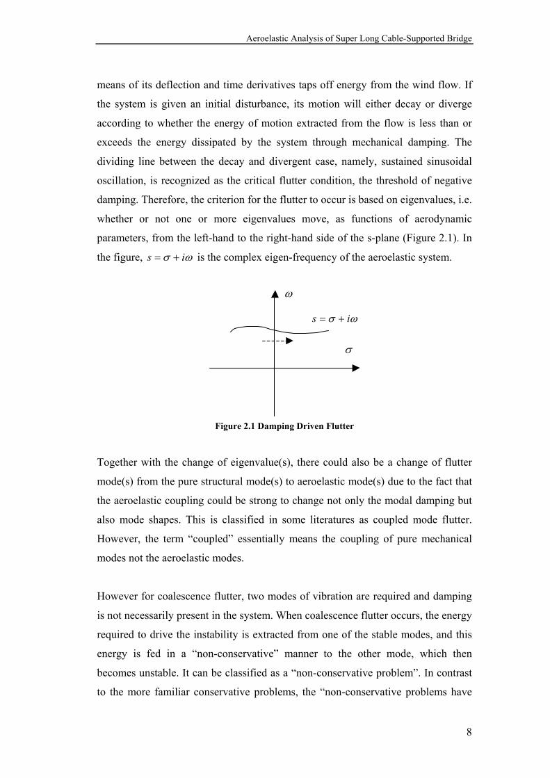
damping. Therefore, the criterion for the flutter to occur is based on eigenvalues, i.e.
whether or not one or more eigenvalues move, as functions of aerodynamic
parameters, from the left-hand to the right-hand side of the s-plane (Figure 2.1). In
the figure, ωσ is += is the complex eigen-frequency of the aeroelastic system.
Figure 2.1 Damping Driven Flutter
Together with the change of eigenvalue(s), there could also be a change of flutter
mode(s) from the pure structural mode(s) to aeroelastic mode(s) due to the fact that
the aeroelastic coupling could be strong to change not only the modal damping but
also mode shapes. This is classified in some literatures as coupled mode flutter.
However, the term “coupled” essentially means the coupling of pure mechanical
modes not the aeroelastic modes.
However for coalescence flutter, two modes of vibration are required and damping
is not necessarily present in the system. When coalescence flutter occurs, the energy
required to drive the instability is extracted from one of the stable modes, and this
energy is fed in a “non-conservative” manner to the other mode, which then
becomes unstable. It can be classified as a “non-conservative problem”. In contrast
to the more familiar conservative problems, the “non-conservative problems have
σ
ω
ωσ is +=
Aeroelastic Analysis of Super Long Cable-Supported Bridge
9
non-self-adjoint characteristics and are inherently unstable. If we define the set of
aeroelastically influenced stiffness matrix as a family of matrices depending on
parameters e.g. reduced frequency, coalescence flutter is defined by the bifurcation
position of the matrix family in a matrix bundle1.
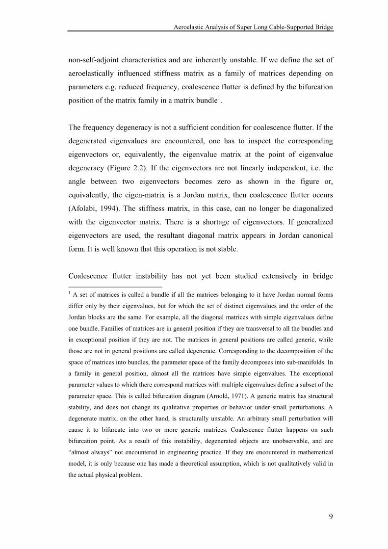
The frequency degeneracy is not a sufficient condition for coalescence flutter. If the
degenerated eigenvalues are encountered, one has to inspect the corresponding
eigenvectors or, equivalently, the eigenvalue matrix at the point of eigenvalue
degeneracy (Figure 2.2). If the eigenvectors are not linearly independent, i.e. the
angle between two eigenvectors becomes zero as shown in the figure or,
equivalently, the eigen-matrix is a Jordan matrix, then coalescence flutter occurs
(Afolabi, 1994). The stiffness matrix, in this case, can no longer be diagonalized
with the eigenvector matrix. There is a shortage of eigenvectors. If generalized
eigenvectors are used, the resultant diagonal matrix appears in Jordan canonical
form. It is well known that this operation is not stable.
Coalescence flutter instability has not yet been studied extensively in bridge 1 A set of matrices is called a bundle if all the matrices belonging to it have Jordan normal forms
differ only by their eigenvalues, but for which the set of distinct eigenvalues and the order of the
Jordan blocks are the same. For example, all the diagonal matrices with simple eigenvalues define
one bundle. Families of matrices are in general position if they are transversal to all the bundles and
in exceptional position if they are not. The matrices in general positions are called generic, while
those are not in general positions are called degenerate. Corresponding to the decomposition of the
space of matrices into bundles, the parameter space of the family decomposes into sub-manifolds. In
a family in general position, almost all the matrices have simple eigenvalues. The exceptional
parameter values to which there correspond matrices with multiple eigenvalues define a subset of the
parameter space. This is called bifurcation diagram (Arnold, 1971). A generic matrix has structural
stability, and does not change its qualitative properties or behavior under small perturbations. A
degenerate matrix, on the other hand, is structurally unstable. An arbitrary small perturbation will
cause it to bifurcate into two or more generic matrices. Coalescence flutter happens on such
bifurcation point. As a result of this instability, degenerated objects are unobservable, and are
“almost always” not encountered in engineering practice. If they are encountered in mathematical
model, it is only because one has made a theoretical assumption, which is not qualitatively valid in
the actual physical problem.

Aeroelastic Analysis of Super Long Cable-Supported Bridge
10
engineering. Therefore, most of the past and current works concentrated on the
prediction of the negative damping boundary with or without considering the
change of pure structural modes to aeroelastic modes.
Figure 2.2 Coalescence Flutter 5 Buffeting
Buffeting is defined as the unsteady loading of a structure by velocity fluctuations
in the oncoming flow. If these velocity fluctuations are clearly associated with the
turbulence shed from the wake of an upstream body, the unsteady loading is
referred to as wake buffeting. However, the buffeting force is usually due to the
atmospheric turbulence.
In this study, the work is focused on flutter instability, i.e. the identification of the
flutter derivative model for self-exited forces on the bridge deck and the prediction
of the damping driven (single mode) flutter boundary. In the following part, some
related work based on flutter derivative models done in the past decades on long
span bridges are introduced. First, there is a review of some historical studies on
thin airfoils.
900
00
Aerodynamic Parameter
Non
-Dim
ensi
onal
Eig
enva
lues
A
ngle
Bet
wee
n Ei
genv
ecto
rs
Aeroelastic Analysis of Super Long Cable-Supported Bridge
11
2.2 Thin Airfoil Aeroelasticity
The aerodynamic forces acting on a thin airfoil undergoing complex sinusoidal
motion h and α : tiehh ω
0= (2.2.1)
tie ωαα 0= (2.2.2)
in two-dimensional incompressible flow are given by Theodorsen (1935) from basic
principles of potential flow theory. The expressions for hL and αM are linear in h ,
α and their first and second derivatives:
))21()((2)(2 ααπρααπρ &&&&&&& abhUkUCbahUbL −++−−+−= (2.2.3)
−+++
+
−++−−=
ααπρ
ααπρ
&&
&&&&&
)21()()
21(2
)81()
21(
2
222
abhUkCaUb
hababUbabM (2.2.4)
where Ubk /ω= is the reduced frequency, b is the half-chord of the airfoil, ab is
the distance between the mid chord and the rotation point, ρ is the air density, U is
the flow velocity and ω is the circular frequency of oscillation. The complex
function )()()( kiGkFkC += is Theodorsen’s circulation function. The coefficients
in the expression, referred to as aerodynamic coefficients, are defined in terms of
two theoretical functions )(kF and )(kG ,
[ ] [ ][ ] [ ]201
201
011011
)()()()()()()()()()()(
kJkYkYkJkJkYkYkYkJkJkF
−++−++
= (2.2.5)
[ ] [ ]2012
01
0101
)()()()()()()()()(
kJkYkYkJkJkJkYkYkG
−+++
−= (2.2.6)

Aeroelastic Analysis of Super Long Cable-Supported Bridge
12
in which 10 , JJ are Bessel functions of the first kind, 10 ,YY are Bessel functions of
the second kind.
This equation is in frequency and time domain hybrid format. There were also
efforts to transform the expression from unsteady aeroelastic force to time domain.
Wagner (1925) showed that the lift evolution with dimensionless time bUts /=
acting on a theoretical flat airfoil given a step function change 0α in angle of attack
is given by
)()2)(2(21
02 sbUL φαπρ= (2.2.7)
where )(sφ is the Wagner function:
∫∞
∞−= dke
kkC
is iks)(
21)(π
φ . (2.2.8)
)(kC is the Theodorsen circulation function and k is the reduced frequency.
For arbitrary motion, the lift force is given as
σσφσαπρ dsbUsLs
∫ ∞−−′−= )()()2)(2(
21)( 4/3
2 (2.2.9)
where )(4/34/3 sdsd αα =′ and 4/3α is the effective angle of attack,
−++=
Uab
Uh ααα
&&)
21(4/3 . (2.2.10)
h& is the vertical velocity and ab is the distance from the mid-chord to the reference
point at which deflection and rotation angle are measured.
Aeroelastic Analysis of Super Long Cable-Supported Bridge
13
Jones [1940] introduced rational approximation of the unsteady loads on a typical
airfoil section in incompressible flow in order to ease the difficulties in flutter
stability analysis. In dimensionless time domain,
ss ees 300.00455.0 335.0165.01)( −− −−≅φ . (2.2.11)
Kussner (1936) considered the problem of an airfoil with forward flight velocity
U penetrating a uniform vertical gust of infinite downstream extent and vertical
velocity 0w . He determined the lift due to this circumstance to evolve according to
the description:
)()2(21)( 02 s
UwBUsL ψπρ= (2.2.12)
with L and 0w considered positive upward, and )(sψ is the Kussner function
defined approximately by Jones(1941)
ss ees −− −−≅ 500.0500.01)( 130.0ψ . (2.2.13)
For the gust of arbitrary velocity distribution )(sw , the lift generated by an airfoil
advancing through it will be given as
∫ ∞−−′=
sdswUBsL σσψσπρ )()()( . (2.2.14)
For a gust velocity distribution that is sinusoidal of the form iksewsw 0)( = , Sears
(1941) derived the corresponding oscillatory lift on the airfoil in the form
iksekUwBUsL )()2(
21)( 02 Θ= πρ (2.2.15)
Aeroelastic Analysis of Super Long Cable-Supported Bridge
14
where )(kΘ is a complex frequency-domain function known as Sears function. It is
clear that the Kussner function and Sears function are a Fourier transform pair:
∫∞ −=Θ0
)()( σσψ σ deikk ik . (2.2.16)
It was further shown by Fung (1955) that Sears function )(kΘ is related to
Theodorsen circulation function )(kC as follows
[ ] )()()()()( 110 kiJkJkJkCk +−=Θ (2.2.17)
where 0J and 1J are Bessel functions of argument k .
Spectral forms of )(sL are also available, but will not be reviewed.
In the case of bridge engineering, however, because of the complexity of the bluff
body aerodynamics, special considerations are needed for the formulation of self-
excited forces on bridge decks.
2.3 Aeroelastic and Aerodynamic Forces on Long-Span
Cable-Supported Bridge Decks
A basic task in the study of the bridge aeroelasticity is to formulate the forces of
wind on the structure. The total lift force L, drag force D and moment M are
decomposed to motion dependent force and motion independent force: aeroelastic
forces (ae) and buffeting force (b):
bae LLL += (2.3.1)
bae DDD += (2.3.2)
bae MMM += (2.3.3)
Aeroelastic Analysis of Super Long Cable-Supported Bridge
15
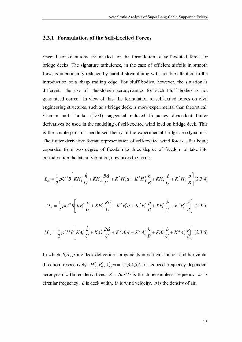
2.3.1 Formulation of the Self-Excited Forces
Special considerations are needed for the formulation of self-excited force for
bridge decks. The signature turbulence, in the case of efficient airfoils in smooth
flow, is intentionally reduced by careful streamlining with notable attention to the
introduction of a sharp trailing edge. For bluff bodies, however, the situation is
different. The use of Theodorsen aerodynamics for such bluff bodies is not
guaranteed correct. In view of this, the formulation of self-exited forces on civil
engineering structures, such as a bridge deck, is more experimental than theoretical.
Scanlan and Tomko (1971) suggested reduced frequency dependent flutter
derivatives be used in the modeling of self-excited wind load on bridge deck. This
is the counterpart of Theodorsen theory in the experimental bridge aerodynamics.
The flutter derivative format representation of self-excited wind forces, after being
expanded from two degree of freedom to three degree of freedom to take into
consideration the lateral vibration, now takes the form:
+++++=
BpHK
UpKH
BhHKHK
UBKH
UhKHBULae
*6
2*5
*4
2*3
2*2
*1
2
21 &&&
ααρ (2.3.4)
+++++=
BhPK
UhKP
BpPKPK
UBKP
UpKPBUDae
*6
2*5
*4
2*3
2*2
*1
2
21 &&&
ααρ (2.3.5)
+++++=
BpAK
UpKA
BhAKAK
UBKA
UhKABUM ae
*6
2*5
*4
2*3
2*2
*1
2
21 &&&
ααρ (2.3.6)
In which ph ,,α are deck deflection components in vertical, torsion and horizontal
direction, respectively. 6,5,4,3,2,1,,, *** =mAPH mmm are reduced frequency dependent
aerodynamic flutter derivatives, UBK /ω= is the dimensionless frequency. ω is
circular frequency, B is deck width, U is wind velocity, ρ is the density of air.

Aeroelastic Analysis of Super Long Cable-Supported Bridge
16
The flutter derivative model works only for sinusoidal or exponentially modified
sinusoidal motion with decay rate less then 20%. Among the flutter derivatives, *1H , *
2H , *5H , *
1A , *2A , *
5A , *1P , *
2P and *5P describe aerodynamic forces in phase
with bridge deck velocity. Therefore they are damping terms. *3H , *
4H , *6H , *
3A ,
*4A , *
6A , *3P , *
4P and *6P describe aeroelastic forces in phase with the bridge deck
displacement. They are stiffness terms. A better understanding of the flutter
derivatives is due to quasi-static theory in the following way (Simiu and Scanlan,
1996). The static wind force coefficients are defined as non-dimensional numbers:
BlULCL 2
2ρ
= , BlU
DCD 2
2ρ
= , lBU
MCM 22
2ρ
= (2.3.7)
where MDL CCC ,, are mean lift, drag and moment force coefficients respectively
L is lift force, D is drag force, M is moment, B model width, U is wind speed, l is
model length, ρ is the density of air.
For small angle of attack α ,
Uh&
=α or UBαα&
= (2.3.8)
the typical term in equation (2.3.4~2.3.6) can be viewed in the classical patterns of
expressions for aerodynamic lift force per unit span.
αα
ρρddCBUCBUL L
L )2(21)2(
21 22 ≅= (2.3.9)
Formally, term *1KH is analogous of the lift coefficient derivative αddCL / . These
flutter derivatives should be referred to as motional derivatives and they go over
into steady-state derivatives only for zero frequency, i.e. 0→K . The general
expressions of flutter derivatives in the form of quasi-static theory are as follows:

Aeroelastic Analysis of Super Long Cable-Supported Bridge
17
'*1 2
1LC
nBUH
=
π (2.3.10)
'2
2*3 4
1LC
nBUH
=
π (2.3.11)
LCnBUH
−=
π1*
5 (2.3.12)
'*1 2
1MC
nBUA
=
π (2.3.13)
'2
2*3 4
1MC
nBUA
=
π (2.3.14)
MCnBUA
−=
π1*
5 (2.3.15)
DCnBUP
−=
π1*
1 (2.3.16)
'*2 2
1DC
nBUP
=
π (2.3.17)
'2
2*
3 41
DCnBUP
=
π (2.3.18)
'*5 2
1DC
nBUP
=
π (2.3.19)
where ''' ,, MDL CCC are corresponding first derivatives of force coefficients with
respect to angle of attack α at 0=α ; n is structural frequency.
Like the researchers in the airfoil aeroelasticity, civil engineering researchers are
trying to expand the time-frequency domain hybrid format model to time domain. A
more general understanding of the unsteady aeroelastic force is found by
recognizing that the indicial function expression can be seen as a modification of
quasi-static nominal form of wind force under turbulent condition. The wind lift
Aeroelastic Analysis of Super Long Cable-Supported Bridge
18
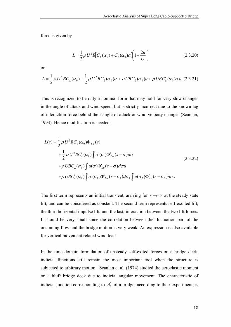
force is given by
[ ]
+′+=
UuCCBUL LL
21)()(21
002 αααρ (2.3.20)
or
uCUBuUBCCBUBCUL LLLL ααραρααραρ )()()(21)(
21
0002
02 ′++′+= (2.3.21)
This is recognized to be only a nominal form that may hold for very slow changes
in the angle of attack and wind speed, but is strictly incorrect due to the known lag
of interaction force behind their angle of attack or wind velocity changes (Scanlan,
1993). Hence modification is needed:
∫∫∫
∫
−Φ′−Φ′′+
−Φ′+
−Φ′′+
Φ=
s
Lu
s
LL
s
LuL
s
LL
LL
dsudsCUB
udsuUBC
dsCBU
sBCUsL
0 2220 1110
00
002
02
)()()()()(
)()()(
)()()(21
)()(21)(
σσσσσσααρ
σσσαρ
σσσααρ
αρ
α
α
α
(2.3.22)
The first term represents an initial transient, arriving for ∞→s at the steady state
lift, and can be considered as constant. The second term represents self-excited lift,
the third horizontal impulse lift, and the last, interaction between the two lift forces.
It should be very small since the correlation between the fluctuation part of the
oncoming flow and the bridge motion is very weak. An expression is also available
for vertical movement related wind load.
In the time domain formulation of unsteady self-exited forces on a bridge deck,
indicial functions still remain the most important tool when the structure is
subjected to arbitrary motion. Scanlan et al. (1974) studied the aeroelastic moment
on a bluff bridge deck due to indicial angular movement. The characteristic of
indicial function corresponding to *2A of a bridge, according to their experiment, is

Aeroelastic Analysis of Super Long Cable-Supported Bridge
19
strongly different from those of the corresponding functions of airfoils. They
showed the relationship between the flutter derivatives and the indicial function by
recognizing that for a sinusoidal motion, the Duhamel integral is of the nature of a
Fourier transform and the inverse transform of frequency domain expression should
then produce the indicial function.
The direct measurement of indicial function is neither easy, nor conventional in the
sense of modern dynamic experiment techniques. Yoshimura and Nakamura (1979)
suggested, in their study on the measurement of the indicial aerodynamic moment
response of moving bluff prismatic sections in still air, that since the aeroelastic
moment arises from the relative motion between the fluid and body, it might be
expressed more conveniently by the time derivatives of the state variables. By
assuming the superposition of small disturbances to a linear aerodynamic system,
the moment due to the angular motion is decomposed into two parts, namely the
moment due to the angle of attack )(sα and the angular velocity of the body axis
relative to the fixed coordinated )(sq :
constconstq sqMsMsqsM == += ααα ))(())(())(),(( (2.3.23)
and the indicial dynamic moment response is also decomposed into two terms:
dsdss q /)()( Φ+Φ=Φ αθ . (2.3.24)
The first term is the indicial aerodynamic moment response for the angle of attack
motion and the second term is the indicial aerodynamic moment response for the
angular velocity motion. Three types of indicial motion were used. In the reported
study, it was found that the contribution of the angle of attack motion dominates,
while the second term contribution to the overall indicial function is small and
negligible.
Aeroelastic Analysis of Super Long Cable-Supported Bridge
20
2.3.2 Buffeting Forces
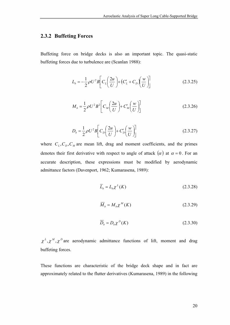
Buffeting force on bridge decks is also an important topic. The quasi-static
buffeting forces due to turbulence are (Scanlan 1988):
( )
+′+
−=
UwCC
UuCBUL DLLb
221 2ρ (2.3.25)
′+
=
UwC
UuCBUM MMb
221 22ρ (2.3.26)
′+
=
UwC
UuCBUD DDb
221 2ρ (2.3.27)
where MDL CCC ,, are mean lift, drag and moment coefficients, and the primes
denotes their first derivative with respect to angle of attack ( )α at 0=α . For an
accurate description, these expressions must be modified by aerodynamic
admittance factors (Davenport, 1962; Kumarasena, 1989):
)(KLL Lbb χ= (2.3.28)
)(KMM Mbb χ= (2.3.29)
)(KDD Dbb χ= (2.3.30)
DML χχχ ,, are aerodynamic admittance functions of lift, moment and drag
buffeting forces.
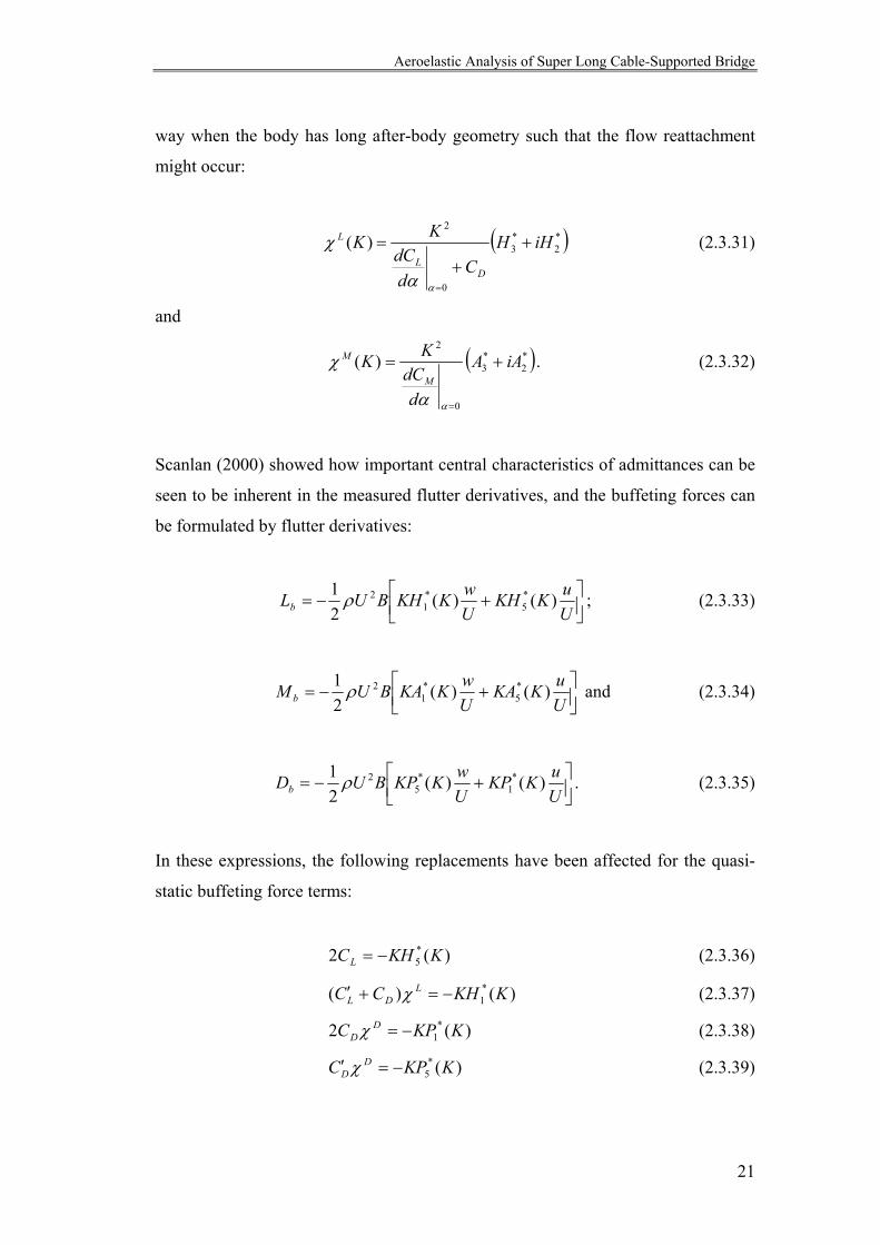
These functions are characteristic of the bridge deck shape and in fact are
approximately related to the flutter derivatives (Kumarasena, 1989) in the following
Aeroelastic Analysis of Super Long Cable-Supported Bridge
21
way when the body has long after-body geometry such that the flow reattachment
might occur:
( )*2
*3
0
2
)( iHHC
ddC
KKD
L
L ++
=
=αα
χ (2.3.31)
and
( )*2
*3
0
2
)( iAA
ddC
KKM
M +=
=αα
χ . (2.3.32)
Scanlan (2000) showed how important central characteristics of admittances can be
seen to be inherent in the measured flutter derivatives, and the buffeting forces can
be formulated by flutter derivatives:
+−=
UuKKH
UwKKHBULb )()(
21 *
5*1
2ρ ; (2.3.33)
+−=
UuKKA
UwKKABUM b )()(
21 *
5*1
2ρ and (2.3.34)
+−=
UuKKP
UwKKPBUDb )()(
21 *
1*
52ρ . (2.3.35)
In these expressions, the following replacements have been affected for the quasi-
static buffeting force terms:
)(2 *5 KKHCL −= (2.3.36)
)()( *1 KKHCC L
DL −=+′ χ (2.3.37)
)(2 *1 KKPC D
D −=χ (2.3.38)
)(*5 KKPC D
D −=′ χ (2.3.39)

Aeroelastic Analysis of Super Long Cable-Supported Bridge
22
)(2 *5 KKAC M
M −=χ (2.3.40)
)(*1 KKAC M
M −=′ χ (2.3.41)
All coefficients on the left are associated with zero angle of attack for a horizontal
wind, or to any other desired reference position. Because these terms are seen to be
functions of K rather than being, in general, simple constants, they reflect
frequency dependency and thus incorporate aerodynamic admittance effects. In
other words, aerodynamic admittance is inherently expressible in this context as a
function of the flutter derivatives.
2.4 Analytical Method in Frequency Domain
In the last several decades, the most significant advances have been made in
understanding aeroelastic phenomena. Most of current efforts are concentrated on
developing methods to alleviate the flutter instability, vortex-induced vibration and
buffeting. Modern approaches to address these issues are based on a combination of
state-of-the-art analytical, numerical and experimental techniques.
2.4.1 Analytical Method For Flutter Analysis
Techniques predicting flutter boundary of cable-supported bridges have been
developing in two parallel ways: one in frequency domain (Davenport 1962;
Scanlan 1978; Jain et al, 1996), the other in time domain (Matsumoto et al. 1994;
Chen et al. 2000). All these methods are developed to solve negative damping
driven flutter, due to the fact that for civil engineering structures, the wind speed is
rare to reach such a high value to bring about coalescence flutter.
Frequency domain analysis has dominated in the past due to the efficiency of
computation, especially when handling the unsteady aeroelastic forces that are
functions of reduced frequency. The nature of flutter analysis is generally a
Aeroelastic Analysis of Super Long Cable-Supported Bridge
23
complex eigenvalue problem, while buffeting analysis is conducted mainly by
mode-by-mode approach ignoring the aerodynamic coupling among modes.
As mentioned in the proceeding paragraph, the flutter instability of cable-supported
bridges is defined with respect to a negative damping threshold. It is reasonable to
postulate that a single mode will approximate the total response. This assumption is
justifiable from observation of the fact that typically just one predominant mode
will become unstable and dominate the flutter response of a three-dimensional
bridge model in the wind tunnel.
The so-called two-degree-of-freedom flutter analysis method supposes that there is
coherence between bending and torsional mode shapes along the span, and does not
consider the possible influence of transverse displacements. The small lack of
coherence between the bending and torsional mode shape in conventional
suspension bridges may have a non-negligible influence on critical wind velocity, as
has already been notice by other authors (Irwin 1979; Scanlan 1987; Lin and Yang
1983; Miyata et al. 1992). This effect is usually more important for shorter bridges
especially for cable-stayed bridges.
Other authors proposed three-dimensional flutter analysis on the basis of flutter
derivatives (Scanlan and Tomko 1971; Scanlan 1989; 1993). The main point in
studying the fully 3D stability consists in taking into consideration the degrees of
freedom in the lateral direction. Then the equations are more difficult to solve, since
the relations between the vertical, rotational and lateral displacement and the
aeroelastic forces become quite complex, as they depend on the deformation
patterns of the full bridge. In any case it will be supposed that there is no
aerodynamic coupling between these forces along the deck, so that the sectional
description will be integrated along the full bridge length to get total forces.
It has been common to use the combination of a set of mechanical modes, namely
the modes of the bridge structure under non-wind condition, as the flutter mode to
perform the flutter analysis. It is clear, however, due to the aeroelastic effects, the

Aeroelastic Analysis of Super Long Cable-Supported Bridge
24
combination of a limited number of the mechanical modes is only an approximation
of what happens in wind. Direct FEM flutter analysis by Miyata and Yamada
(1988), Miyata et al. (1995), and later development of the mode tracing method by
Dung et al. (1996, 1998) could serve as a better representation of the dynamic
behavior of the long-pan bridges in terms of complex flutter mode. Complex
eigenanalysis is made for an integrated system consisting of the 3-D FEM model of
a bridge and the aeroelastic force caused by the wind flow. To solve the complex
mode is an iterative procedure, tracing down the evolution of each aerodynamic
complex mode with step-by-step increment of wind speed. Finite element method is
the most common choice in this circumstance (Miyata, and Yamada 1988; Agar
1988; 1989; Namini 1991; Namini et al. 1992; Starossek 1993). The deck is usually
modeled by beam elements located along the bridge axis. Plate elements could also
be used provided that aeroelastic force is applied along the elastic axis of the deck.
By assuming harmonic oscillation, the self-exited force on a unit length of bridge
deck is incorporated into the element matrix. With the usual FE procedure, the
governing equations of the aeroelastically-influenced structure can be established.
Eignvalues and eigenvectors need to be found by iterative method since the
governing equation is reduced frequency dependent. In one step, a set of natural
frequencies of the aeroelastically-influenced structure is obtained with fixed wind
speed. The procedure repeats with a different wind speed covering the speed range
of interest.
More recently, an efficient scheme for coupled multimode flutter analysis has been
proposed introducing the unsteady self-exited aerodynamic forces in terms of
rational function approximations (Matsumoto et al. 1994; Chen et al. 2000). This
has led to a convenient transformation of the equation into a state space format
independent of reduced frequency. A significant feature of this approach is that an
iterative solution for determining flutter boundary is unnecessary because the
equations are independent of reduced frequency UBK /ω= where ω is the
circular frequency, B is the deck width and U is the wind velocity. In general,
frequency domain methods are restricted to linear structures excited by the
stationary wind load without aerodynamic nonlinearities. To include nonlinearities

Aeroelastic Analysis of Super Long Cable-Supported Bridge
25
of structural and aerodynamic origins, the time domain approach is more
appropriate. Time domain methods, however, involve the transformation of flutter
derivatives into indicial functions, which have inherent deficit, as will be shown in
the thesis. The effectiveness of time domain analysis in calculating buffeting
response depends on the establishment of an effective time domain model for the
self-excited wind force.
In this thesis, the traditional frequency domain analysis will be used for the flutter
instability analysis in chapter 6. Therefore, it will be reviewed in detail in the
following part.
2.4.2 Governing Equations of Flutter
(Jain et al, 1996)
Deck deflection components can be expressed by generalized mode coordinates
)(tiξ . If B is the bridge deck width, ),( txh is vertical displacement, ),( txα is
torsion displacement and ),( txp is lateral displacement. Deck deflections are
expressed in the following forms:
∑=i
ii tBxhtxh )()(),( ξ (2.4.1)
∑=i
ii txtx )()(),( ξαα (2.4.2)
∑=i
ii tBxptxp )()(),( ξ (2.4.3)
in which, )(xhi , )(xiα and )(xpi are dimensionless representations of thi mode in
each direction respectively.
The governing equation for the bridge deck motion can then be deduced as:
)()2( 2 tqI iiiiiiii =++ ξωξωζξ &&& (2.4.4)

Aeroelastic Analysis of Super Long Cable-Supported Bridge
26
The generalized force is defined as
[ ]dxMBDpBLhtphql
iiii ∫ ++=0
),,,( αα , (2.4.5)
where l is the deck span length; the generalized inertia is
( ) ( )∫= zyxdmzyxI ii ,,,,2η (2.4.6)
where iη is the full bridge mode, iω is the circular frequency and iζ is damping
ratio-to-critical and dm is infinite small mass.
The lift force L, drag force D and moment M in the governing equations are
decomposed to motion dependent force and motion independent force: aeroelastic
forces (ae) and buffeting force (b) as in Equation (2.3.1~2.3.3),
Substituting (2.4.5), (2.4.6) into (2.4.4), we have the dimensionless time domain
governing equation for the bridge deck motion:
),( sxQBAI b=+′+′′ ξξξ (2.4.7)
where BUts /= is the dimensionless time; ξ is the generalized coordinate vector; a
prime denotes the derivative with respect to dimensionless time s ; I is the identity
matrix and the general terms of matrix A , B and bQ are
]
[2
2)(
*5
*2
*1
*5
*2
*1
*5
*2
*1
4
jijijijiji
jijijiji
phhpp
ppphhhhi
ijiiij
GAGAGAGPGP
GPGHGHGHI
lKBKkA
ααααα
αρδζ
+++++
+++−= (2.4.8)
Aeroelastic Analysis of Super Long Cable-Supported Bridge
27
]
[2
)(
*6
*4
*3
*6
*4
*3
*6
*4
*3
242
jijijijiji
jijijiji
phhppp
pphhhhi
ijiij
GAGAGAGPGP
GPGHGHGHIlKBKkB
αααα
ααρδ
+++++
+++−= (2.4.9)
∫ ++=l
ibibibi
b ldxsxMpsxDhsxL
IlBsxQ
i 0
4
),(),(),(2
),( αρ (2.4.10)
where UBK /ω= is the reduced frequency and UBK ii /ω= is the reduced
frequency of mode i , *** ,, mmm PAH , )6,,1( L=m are flutter derivatives and ijδ is the
Kronecker delta function defined as:
≠=
=jiji
ij 01
δ . (2.4.11)
The modal integrals ji srG are obtained by integration over the deck, which is the
primarily aerodynamic load source
∫=l
jisr ldxxsxrG
ji 0)()( (2.4.12)
where iii phr ,= or iα ; jjj phs ,= or jα .
Note that the off-diagonal terms in equation (2.4.7) represent the aeroelastic
coupling through the flutter derivatives and mechanical coupling through the cross
mode integrals among different modes.
The new equation is Fourier transformed in to reduced frequency ( K ) domain
(Scanlan and Jones 1990) by
∫∞ −=
0)()( dsesfKf iks (2.4.13)
and is represented as

Aeroelastic Analysis of Super Long Cable-Supported Bridge
28
bQE =ξ (2.4.14)
where ξ and bQ are Fourier-transformed vectorsξ and bQ , respectively.
The general term of the impedance matrix is
)()(2 KBKiKAKE ijijijij ++−= δ (2.4.15)
where 1−=i .
The flutter condition is then defined as the aeroelasctically influenced eigenvalue
problem:
0=E . (2.4.16)
It is clear that the buffeting terms do not affect flutter stability. However it is
reasonable to argue that the turbulence effect on flutter stability can be take into
consideration by measuring the flutter derivatives in turbulent flow. These effects,
as will be shown in the thesis, will need further studies to include “relative
amplitude” effect.
The flutter mode is determined by the vector ξ in the homogeneous equation
0=ξE . (2.4.17)
The nontrivial solution of equation (2.4.16) and (2.4.17) yields the reduced
frequency at which flutter instability occurs and a non-zero vector ξ . This vector
indicates the relative magnitudes of participation structural modes at flutter. It can
be used as a tool to determine the flutter mode.

Aeroelastic Analysis of Super Long Cable-Supported Bridge
29
2.4.3 Buffeting Analysis
(Jain, 1997)
The vector of buffeting forces on the right hand side of Equation (2.4.14) is
=
∫
∫
∫
l
bnn
l
b
l
b
b
ldxF
I
ldxF
I
ldxF
I
lBQ
0
0 22
0 11
4
1
1
1
2M
ρ (2.4.18)
where the integrands in the vector are:
)(),()(),()(),(),( xKxMxpKxDxhKxLKxF ibibibbi α++= (2.4.19)
The buffeting force may include admittance functions. The power spectral density
(PSD) matrix is obtained by multiplying bQ and its complex conjugate transpose
vector *bQ :
=
∫ ∫∫ ∫
∫ ∫∫ ∫
l l BAbnbn
nn
l l BAbbn
n
l l BAbnb
n
l l BAbb
bb
ldx
ldxFF
IIldx
ldxFF
II
ldx
ldxFF
IIldx
ldxFF
II
UlBQQ
0 0
*
0 0
*1
1
0 0
*1
10 0
*11
1124
*
11
11
2L
MOM
L
ρ , (2.4.20)
where a ‘ * ’ denotes complex conjugate transpose.
Expressed in generalized displacement ξ (2.4.7), the PSD matrix becomes:
1**1 ][)( −−= EQQEKS bbξξ . (2.4.21)
Hence, physical displacement PSD is obtained.
Aeroelastic Analysis of Super Long Cable-Supported Bridge
30
Take vertical displacement as an example:
∑∑=i j
jiBjAiBAhh KSxhxhBKxxS )()()(),,( 2ξξ (2.4.22)
By integrating respective PSDs the mean-square value of the displacement can be
found:
∫∞
=0
2 ),,(),( dnnxxSxx BAhhBAhhσ . (2.4.23)
A covariance matrix for vertical displacement is thus obtained. Torsion and lateral
displacement can be treated in the same manner. The statistics of the displacements
can be calculated.
Summary
Besides the historical work in airfoil aerodynamics, selected research was obtained
from the literature on bridge aerodynamics for presentation in this chapter. Flutter
derivative models and analytical methods for flutter prediction and buffeting
response estimation are reviewed. Frequency domain methods are paid attention to.
Aeroelastic Analysis of Super Long Cable-Supported Bridge
31
CHAPTER THREE
Wind Tunnel Experiment to Extract
Flutter Derivatives
Abstract
The wind tunnel experiment remains the practical means to study the aeroelastic
behavior of bridges. In this part, methods of wind tunnel experiment to measure
flutter derivatives are reviewed; experimental design for the research is presented;
the experimental procedure is introduced and limitations of the experiment
discussed. Preliminary results are also presented.

Aeroelastic Analysis of Super Long Cable-Supported Bridge
32
3.1 Introduction
Wind tunnel experiments are usually used to evaluate the aerodynamic behavior of
bridge decks, as the reliable prediction based on purely theoretical methods has
proven hard to obtain. The confidence of wind tunnel testing has grown not only
because the principles of dynamic similarity lead one to expect good predictions
from wind tunnel models but also because good correspondence has been observed
between model and full-scale in a number of specific cases. While wind tunnel
models are frequently used as direct physical analog of full-scale structures, they
are now often employed more as a tool for obtaining values of empirical parameters
needed by various theories. An example of such theory is the semi-theoretical
flutter derivative model for the prediction of flutter boundary of cable-supported
bridges (Scanlan 1971, Scanlan & Jones 1990, Jain et al. 1996). The model does not
attempt to describe the detailed flow patterns around the bridge deck, and the
corresponding aerodynamic forces, but rather to provide a theoretical framework,
which contains a number of empirical parameters, flutter derivatives, describing the
wind forces. Although they are semi-empirical in nature, they can be helpful in
understanding the bridge behavior especially in more complex cases where the
bridge modes of vibration are complex. Wind tunnel experiments, primarily
sectional model testing, are used to quantify the flutter derivatives.
A sectional model is a span-wise representative segment of a full-scale structure.
The model itself is rigid, but is elastically suspended between end plates. The
model-to-full-scale ratio is typically in the range 30:1=Lλ to 200:1 . A sectional
model can be used in airflow as
1 An almost immobile object to measure time-average load for the whole
model or transducer forces and pressure data including everything except for
motion dependency;
2 Forced oscillating model to measure time series of driving forces and input
motion, plus possible pressure or
3 Free vibrating model to measure the displacement time series and/or
transducer forces.
Aeroelastic Analysis of Super Long Cable-Supported Bridge
33
The state-of-the-art use of sectional model is different from that used earlier
(Farquharson 1949). In the past, full-scale response was estimated from sectional
model testing directly. This estimation was at times of questionable reliability.
3.1.1 Similitude in the Experiment (Tanaka 1992)
The wind tunnel experiment is to correctly model the behavior of wind flow in a
certain space or area and its interaction between the geometrical and/or mechanical
characteristics of the boundaries of the field of concern. Based on Buckingham’s Pi-
theorem, it is required that a set of dimensionless parameters be invariant in the
model and prototype and with them, the governing equations also be dimensionless.
These parameters consist of suitable combinations of the reference quantities.
Various boundary conditions have also to be maintained in a dimensionless form.
Theoretically speaking, all of the dimensionless parameters in the prototype must be
duplicated in the model. However, almost inevitably, complete duplication of these
parameters is impracticable. As a mater of fact, all the requirements can be satisfied
exactly only when model and prototype are identical. Hence, decision must be made
as to which parameters can be relaxed or distorted to what extent for each testing
based on the understanding of the phenomenon and knowledge of dominant
parameters. Only a part of the process can be simulated to clarify the unknown
mechanism. The deficit part has to rely on analytical means for its solution.
The similitude requirements for testing have been well established and practiced for
a long time. The tradition of the aeroelastic model testing requires the similarities of
geometry and reduced frequencies (Cauchy Number) to be met (Hjorth-Hansen
1992). It is worthwhile, however, to have a review on all the dimensionless
numbers.
Cauchy Number is defined as the ratio of elastic force to the fluid inertia force:

Aeroelastic Analysis of Super Long Cable-Supported Bridge
34
2/ UECa ρ= . In aeroelastic testing of a sectional model, the Cauchy number is
usually rewritten to fBU / , where U is a short time average of wind speed; f is an
eigen-frequency of un-damped motion in some reference condition; B is the a
reference length. In most wind tunnel tests, rather than the original Cauchy number,
reduced velocity ( fBU / ) is much easier to use.
Reynolds number can be defined as the ratio of the fluid inertia force to the fluid
viscous force. In most wind tunnel tests, it is impractical to satisfy the Reynolds
number similitude. Indeed, the viscous force is usually of smaller magnitude and
relatively unimportant compared with the fluid inertia force for a large part of the
flow domain, but can be large for the parts close to the boundary. To have a correct
interpretation of the results, the consequences of neglecting the Reynolds number
similitude should be examined carefully, particularly in the case of vortex shedding
about structures with curved surface. Since vortex-shedding formation around such
structures is sensitive to Reynolds number. There is a shift of separation point with
the change of Reynolds number. The critical Reynolds number also dependents on
the surface roughness of the solid boundary and the turbulence level of the
oncoming flow. Civil engineering structures usually have sharp corners, their flow
separation points do not shift and the flow pattern is believed to be less sensitive to
the change of Reynolds number. However, a broad wake after separation from the
upstream corner may reattach to the body surface, depending on the aspect ratio of
the structure. The reattachment results in the reduction of drag force and increase of
Strouhal number in general. The critical body aspect ratio at which this change
occurs depends on Reynolds number as well as the corner radius and the air stream
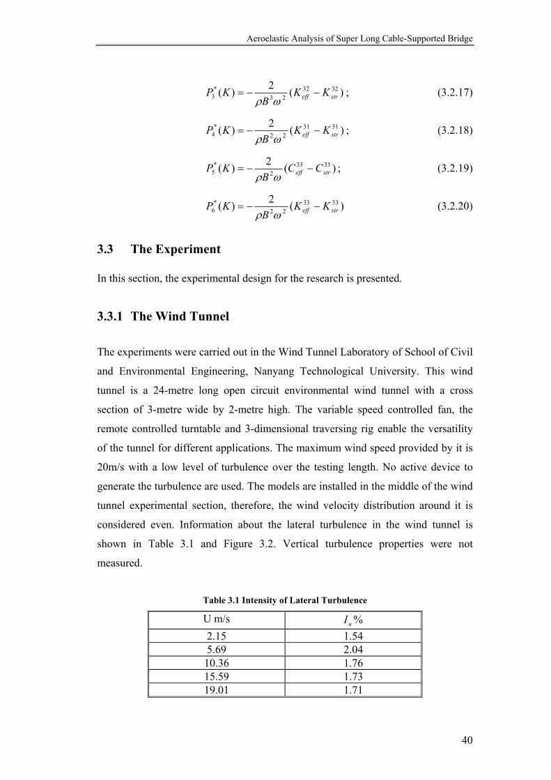
turbulence level. This factor is also affected by the wind tunnel blockage ratio.
As the turbulence effect on the flutter boundary is an important issue, it is essential
to simulate the velocity spectra correctly if the experiment is done with turbulence
effect on the flutter derivatives being taken into consideration. A sectional model
may be exposed to flow of any mean speed profile and to different types of wind
turbulence. A sheared mean speed profile may not really be important for full-scales
with good clearance from water or land, but wind turbulence is presumably very
Aeroelastic Analysis of Super Long Cable-Supported Bridge
35
important. The target values for turbulence intensity may be encircled in the
satisfactory manner, but the flow inevitably contains too much fine-grained
fluctuation and too little at the low-frequency end, corresponding to long wave
eddies approaching the model. Therefore, while some results may hold their value
as reasonably good predictions for full-scale, the buffeting response of the model
will not be linked to that of the full-scale (Hjorth-Hansen 1992). Lack of similarity
of integral length-scales of the turbulent flow is not a unique feature of sectional
models, but rather a common error source for any stand-in for the full-scale.
For a Reynolds number that is large enough to allow turbulent flow, the flow
structures are almost the same for all Reynolds numbers. This is very important
since achieving the similitude of Reynolds number is in any case impractical.
However, Reynolds numbers does play a role in the existence of the inertia sub-
range of energy spectra.
Froude number represents the ratio of fluid inertia forces and vertical gravity or
buoyant forces. Consequently the Froude similitude becomes important when the
gravity predominates the dissipation of air born particles or wind induced response
of cable-supported structures. Although Froude similitude has been widely accepted
and employed for many aeroelastic studies in the past, it is not an essential
requirement unless the gravity or buoyancy plays an important role. In the
experiment of sectional model testing, the restoring force is provided mainly by
elastic force in the spring; the aeroelastic response does not require the Froude
similitude.
Density ratio is referred to the ratio of structural material density to air. In the case
where the model is only an equivalent model, which simply maintains the
geometrical and dynamical characteristics of the prototype, this ratio is thus of no
consequence.
The magnitude of structural damping in the system is obviously an important
parameter for the predication of structural response. The problem, however, is that
Aeroelastic Analysis of Super Long Cable-Supported Bridge
36
its magnitude is not known precisely until the structure has been constructed. As a
mater of fact, even for the existing structure, the magnitude of structural damping is
uncertain because of the difficulty in measuring its value and its dependency on
amplitude.
For the identification of the flutter derivatives, structural damping is not important.
Singh (1997) used additional dampers to increase the stability of very bluff model
when it became unstable under low wind velocity. For the study of vortex-shedding
effects, system damping and mass cannot be overlooked. Peak bending or rotational
amplitudes of beams under vortex-shedding excitations are clearly related to the
damping and mass of the system.
Structural details have significant effects on the flutter derivatives measured in wind
tunnel experiments. This was manifested by Ehsan et al (1993). Therefore, the
design of structure details for the bridge deck model is very important. The rail, for
example, need to be duplicated in such a way that the static force and moment
generated by it in the full scale and the model satisfy the requirement of similarity
in terms of geometric scale factor. The difficulty is that the dimension of the model
is very small and the Reynolds number in the wind tunnel corresponding to its
dimension is rather small, the drag or lift coefficients may have a significant change
if the rail was faithfully duplicated. In practice, instead of a replica of the full-scale
rail, wire mesh is usually used so that similarity requirement can be met. In such a
small dimension, Reynolds number effect on the drag coefficient of the circular
sectioned wire is not large.
End plates are usually used to reduce the end effect. For sectional model, it is
necessary to ensure the flow around it is a two-dimensional flow. However
according to the work of some researchers e.g. Hjorth-Hansen (1992), the end effect
is, hopefully, not significant.
Aeroelastic Analysis of Super Long Cable-Supported Bridge
37
3.1.2 Other Model Types
Besides sectional model, partial and full models are also used for the study on
aeroelastic behavior of cable-supported bridges.
Full models (Irwin, 1992) can simulate turbulent effects, topographic effects, mode
effects and responses during different construction stages. However, they are very
expensive and time consuming to build. Besides, a full model requires that
similarities pertaining to mass distribution, reduced frequency, mechanical damping
and mode shapes be met. Full models are not suitable for the investigation of flutter
mechanisms since the addition of tower and cable has influences on the bridge deck
behavior, making it even difficult to understand the mechanisms of bridge deck
vibrations.
Taut strip models or partial bridge model (Davenport, 1992) is a three dimensional
but simplified representation of the prototype. With properly designed sectional
model mounted on the taut wires or taut tubes stretched between two anchors, it can
match the lowest vertical, horizontal and torsional modes shape and frequency ratio
of the model to those of the prototype.
Because full and partial bridge models are built at too small a scale to present the
small details, they are not good at responding to vortex shedding. Also, vortex-
shedding excitations can happen at quite moderate wind speeds at full-scale which
scale down to very low values on the aeroelastic model in wind tunnel. This can
introduce the unwanted Reynolds number effects on the mean flow and turbulence
(Irwin, 1998).
3.2 Extraction of Flutter Derivatives
Figure (3.1) shows the sectional model and coordinates system for the bridge
section. In the experiment, we will denote the vertical, lateral and rotational
Aeroelastic Analysis of Super Long Cable-Supported Bridge
38
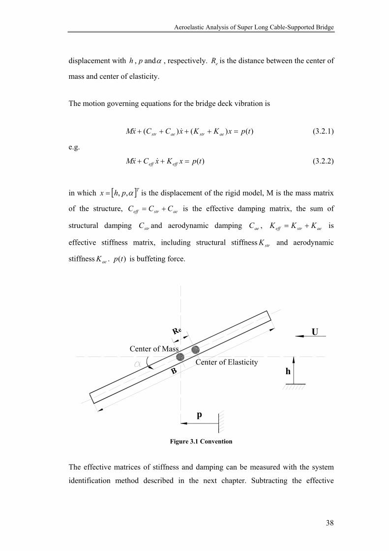
displacement with h , p andα , respectively. eR is the distance between the center of
mass and center of elasticity.
The motion governing equations for the bridge deck vibration is
)()()( tpxKKxCCxM aestraestr =++++ &&& (3.2.1)
e.g.
)(tpxKxCxM effeff =++ &&& (3.2.2)
in which [ ]Tphx α,,= is the displacement of the rigid model, M is the mass matrix
of the structure, aestreff CCC += is the effective damping matrix, the sum of
structural damping strC and aerodynamic damping aeC , aestreff KKK += is
effective stiffness matrix, including structural stiffness strK and aerodynamic
stiffness aeK . )(tp is buffeting force.
B
Re
p
h
U
Center of Mass
Center of Elasticity
Figure 3.1 Convention
The effective matrices of stiffness and damping can be measured with the system
identification method described in the next chapter. Subtracting the effective
Aeroelastic Analysis of Super Long Cable-Supported Bridge
39
matrices by structural matrices, aeroelastic derivatives can be obtained. Flutter
derivatives are as follows:
)(2)( 11112
*1 streff CC
BKH −−=
ωρ; (3.2.3)
)(2)( 12123
*2 streff CC
BKH −−=
ωρ; (3.2.4)
)(2)( 121223
*3 streff KK
BKH −−=
ωρ; (3.2.5)
)(2)( 111122
*4 streff KK
BKH −−=
ωρ; (3.2.6)
)(2)( 13132
*5 streff CC
BKH −−=
ωρ; (3.2.7)
)(2)( 131322
*6 streff KK
BKH −−=
ωρ; (3.2.8)
)(2)( 21213
*1 streff CC
BKA −−=
ωρ; (3.2.9)
)(2)( 22224
*2 streff CC
BKA −−=
ωρ; (3.2.10)
)(2)( 222224
*3 streff KK
BKA −−=
ωρ; (3.2.11)
)(2)( 212123
*4 streff KK
BKA −−=
ωρ; (3.2.12)
)(2)( 23233
*5 streff CC
BKA −−=
ωρ; (3.2.13)
)(2)( 232323
*6 streff KK
BKA −−=
ωρ; (3.2.14)
)(2)( 31312
*1 streff CC
BKP −−=
ωρ; (3.2.15)
)(2)( 32323
*2 streff CC
BKP −−=
ωρ; (3.2.16)
Aeroelastic Analysis of Super Long Cable-Supported Bridge
40
)(2)( 323223
*3 streff KK
BKP −−=
ωρ; (3.2.17)
)(2)( 313122
*4 streff KK
BKP −−=
ωρ; (3.2.18)
)(2)( 33332
*5 streff CC
BKP −−=
ωρ; (3.2.19)
)(2)( 333322
*6 streff KK
BKP −−=
ωρ (3.2.20)
3.3 The Experiment In this section, the experimental design for the research is presented.
3.3.1 The Wind Tunnel
The experiments were carried out in the Wind Tunnel Laboratory of School of Civil
and Environmental Engineering, Nanyang Technological University. This wind
tunnel is a 24-metre long open circuit environmental wind tunnel with a cross
section of 3-metre wide by 2-metre high. The variable speed controlled fan, the
remote controlled turntable and 3-dimensional traversing rig enable the versatility
of the tunnel for different applications. The maximum wind speed provided by it is
20m/s with a low level of turbulence over the testing length. No active device to
generate the turbulence are used. The models are installed in the middle of the wind
tunnel experimental section, therefore, the wind velocity distribution around it is
considered even. Information about the lateral turbulence in the wind tunnel is
shown in Table 3.1 and Figure 3.2. Vertical turbulence properties were not
measured.
Table 3.1 Intensity of Lateral Turbulence
U m/s %uI 2.15 1.54 5.69 2.04 10.36 1.76 15.59 1.73 19.01 1.71

Aeroelastic Analysis of Super Long Cable-Supported Bridge
41
10-1 100 101 102-18
-16
-14
-12
-10
-8
-6
-4
Frequency (Hz)
Pow
er S
pect
ral D
ensi
ty (d
B/H
z)
Figure 3.2 Power Spectral Density of Lateral Turbulence U=17.4m/s
3.3.2 Sectional Models
There are two bridge deck sectional models used in the experiment: a bluff twin
deck model and a partially streamline box girder model. They are chosen as
representatives of different types of bridge decks.
1. Model A (Figure 3.3) is a bluff twin deck model with an opening between
the two decks. Configuration of the model follows the design of Ting Kau
Bridge1. The scale ratio for the model is 1:80 to allow for adequate detailing
1 The Ting Kau Bridge (King et al, 1997) with its 1177m length is one of the longest cable-stayed bridges in the world. It consists of two main span of 448m and 475m and two side spans and provides a vital link in Hong Kong’s new Route 3, connecting Hong Kong Island, Kowloon and the new airport on Lantau to the New Territories and the border to Mainland. The deck has a varying chord with a minimum of 42.28m excluding fairings, and is separated into two carriageways. Each carriage way has a varying a chamber of approximately 2.5% with two longitudinal L-shaped edge girders, and I-shaped cross beams every 4.5m. Every 13.5m cross beams extend to connect with the other carriageway across at 5.26m void. The deck is very slender with a very high chord to depth ratio of approximately 25, making it potentially susceptible to aerodynamic actions. Since the bridge is situated in a typhoon area it will during its lifetime be subjected to very strong wind. It is thus important to establish the relationship between wind actions and bridge response. Furthermore, because of its slender section and bluff edges the aerodynamic stability is of great concern.
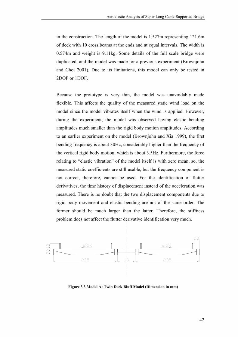
Aeroelastic Analysis of Super Long Cable-Supported Bridge
42
in the construction. The length of the model is 1.527m representing 121.6m
of deck with 10 cross beams at the ends and at equal intervals. The width is
0.574m and weight is 9.11kg. Some details of the full scale bridge were
duplicated, and the model was made for a previous experiment (Brownjohn
and Choi 2001). Due to its limitations, this model can only be tested in
2DOF or 1DOF.
Because the prototype is very thin, the model was unavoidably made
flexible. This affects the quality of the measured static wind load on the
model since the model vibrates itself when the wind is applied. However,
during the experiment, the model was observed having elastic bending
amplitudes much smaller than the rigid body motion amplitudes. According
to an earlier experiment on the model (Brownjohn and Xia 1999), the first
bending frequency is about 30Hz, considerably higher than the frequency of
the vertical rigid body motion, which is about 3.5Hz. Furthermore, the force
relating to “elastic vibration” of the model itself is with zero mean, so, the
measured static coefficients are still usable, but the frequency component is
not correct, therefore, cannot be used. For the identification of flutter
derivatives, the time history of displacement instead of the acceleration was
measured. There is no doubt that the two displacement components due to
rigid body movement and elastic bending are not of the same order. The
former should be much larger than the latter. Therefore, the stiffness
problem does not affect the flutter derivative identification very much.
Figure 3.3 Model A: Twin Deck Bluff Model (Dimension in mm)

Aeroelastic Analysis of Super Long Cable-Supported Bridge
43
2. Model B (Figure3.4) is a partially streamlined box girder deck model with a
wing on each side. Its prototype is the Humber Bridge2. More information of
the bridge can be found in Chapter 6. Length scale is 1:80. Its length is
1.08m; width is 0.35m; weight is 7.7 kg. This model was specifically made
for this study, so it can be tested in 3DOF experiment. The sectional model
is also strong since it has truss structure with a Perspex coat. The frequency
component of the wind load on the stationary model was also not correct,
since the rig was vibrating, which was all unfortunately transmitted to the
load cell.
227355
91
53
92
40 2464
20
92
402464
perspex coat
Figure 3.4 Model B: Streamlined Box Girder Model (Dimension mm)
2 The Humber Bridge connects the towns of Barton and Hessle across the Humber estuary upstream from Hull. Its main span of 1410m was the longest at the time it was built, with side span of 530 and 280m. The argument is not symmetric. It was opened to traffic in July 1981. All three spans at Humber are supported by cables. In the main span and Barton side span, the deck shapes parts of the circles in the vertical plane, tangential to each other at the tower. The Hessel side span is straight. The steel box-sections are 22m wide and 4.5m deep, carrying two traffic lanes each way. The cables consist of 37 strands each of which contains 404 galvanized drawn wires of 5 mm diameter. In each cable above the Hessle side span there are additional 800 wires divided into 4 strands fixed to strand shoes at both the main anchorage and tower saddles. This increased cable area is required to carry the greater tension generated in the steeper slop of this span. For 325.8 m either side of the mid-point of the main span, the hangers are articulated in both lateral and longitudinal directions at deck level; elsewhere, the articulation is in the longitudinal (i.e. about the X-axis) direction only. The towers at Humber are slip-formed concrete box section, 6 by 6 m at the base and 4.5 by 4.5 at the tower tops. The foundation for the Hessle tower is sited on the high-water line, being essentially a reinforced concrete slab 44 by 16 in plan and 11.5 deep. On the Barton side, the tower is supported on a concrete pier, 16 m deep, resting on twin hollow circular caissons each 24 m in diameter.
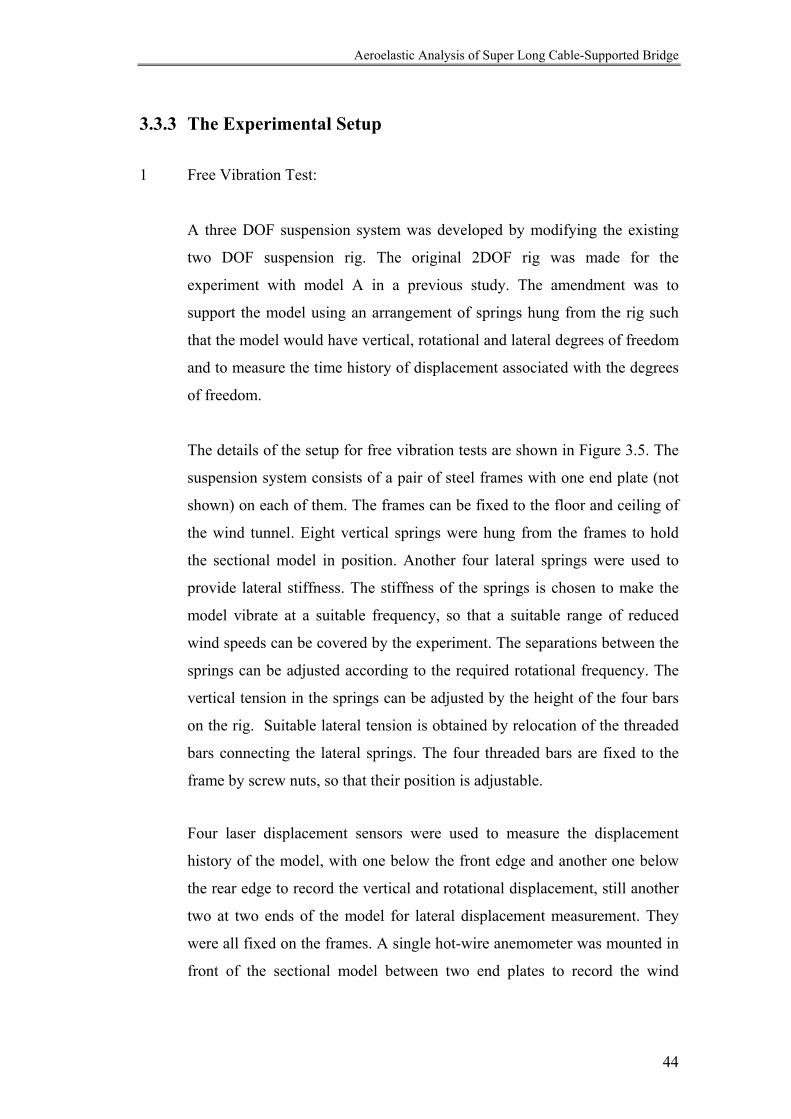
Aeroelastic Analysis of Super Long Cable-Supported Bridge
44
3.3.3 The Experimental Setup
1 Free Vibration Test:
A three DOF suspension system was developed by modifying the existing
two DOF suspension rig. The original 2DOF rig was made for the
experiment with model A in a previous study. The amendment was to
support the model using an arrangement of springs hung from the rig such
that the model would have vertical, rotational and lateral degrees of freedom
and to measure the time history of displacement associated with the degrees
of freedom.
The details of the setup for free vibration tests are shown in Figure 3.5. The
suspension system consists of a pair of steel frames with one end plate (not
shown) on each of them. The frames can be fixed to the floor and ceiling of
the wind tunnel. Eight vertical springs were hung from the frames to hold
the sectional model in position. Another four lateral springs were used to
provide lateral stiffness. The stiffness of the springs is chosen to make the
model vibrate at a suitable frequency, so that a suitable range of reduced
wind speeds can be covered by the experiment. The separations between the
springs can be adjusted according to the required rotational frequency. The
vertical tension in the springs can be adjusted by the height of the four bars
on the rig. Suitable lateral tension is obtained by relocation of the threaded
bars connecting the lateral springs. The four threaded bars are fixed to the
frame by screw nuts, so that their position is adjustable.
Four laser displacement sensors were used to measure the displacement
history of the model, with one below the front edge and another one below
the rear edge to record the vertical and rotational displacement, still another
two at two ends of the model for lateral displacement measurement. They
were all fixed on the frames. A single hot-wire anemometer was mounted in
front of the sectional model between two end plates to record the wind
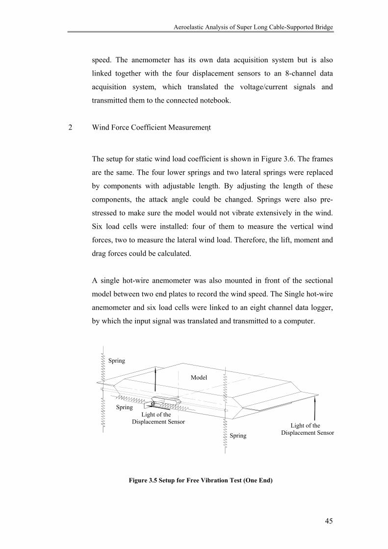
Aeroelastic Analysis of Super Long Cable-Supported Bridge
45
speed. The anemometer has its own data acquisition system but is also
linked together with the four displacement sensors to an 8-channel data
acquisition system, which translated the voltage/current signals and
transmitted them to the connected notebook.
2 Wind Force Coefficient Measurement
The setup for static wind load coefficient is shown in Figure 3.6. The frames
are the same. The four lower springs and two lateral springs were replaced
by components with adjustable length. By adjusting the length of these
components, the attack angle could be changed. Springs were also pre-
stressed to make sure the model would not vibrate extensively in the wind.
Six load cells were installed: four of them to measure the vertical wind
forces, two to measure the lateral wind load. Therefore, the lift, moment and
drag forces could be calculated.
A single hot-wire anemometer was also mounted in front of the sectional
model between two end plates to record the wind speed. The Single hot-wire
anemometer and six load cells were linked to an eight channel data logger,
by which the input signal was translated and transmitted to a computer.
Figure 3.5 Setup for Free Vibration Test (One End)
Spring
Light of the Displacement Sensor
Spring
Model
Light of the Displacement SensorSpring
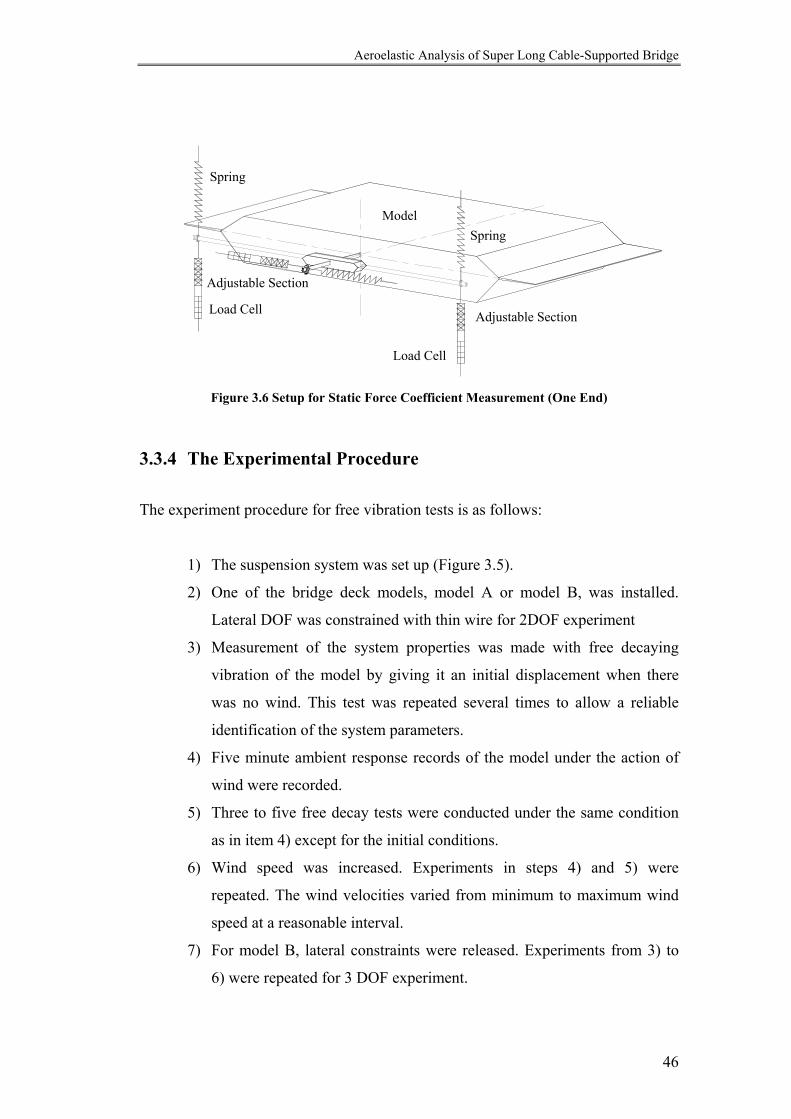
Aeroelastic Analysis of Super Long Cable-Supported Bridge
46
Figure 3.6 Setup for Static Force Coefficient Measurement (One End)
3.3.4 The Experimental Procedure
The experiment procedure for free vibration tests is as follows:
1) The suspension system was set up (Figure 3.5).
2) One of the bridge deck models, model A or model B, was installed.
Lateral DOF was constrained with thin wire for 2DOF experiment
3) Measurement of the system properties was made with free decaying
vibration of the model by giving it an initial displacement when there
was no wind. This test was repeated several times to allow a reliable
identification of the system parameters.
4) Five minute ambient response records of the model under the action of
wind were recorded.
5) Three to five free decay tests were conducted under the same condition
as in item 4) except for the initial conditions.
6) Wind speed was increased. Experiments in steps 4) and 5) were
repeated. The wind velocities varied from minimum to maximum wind
speed at a reasonable interval.
7) For model B, lateral constraints were released. Experiments from 3) to
6) were repeated for 3 DOF experiment.
Spring
Load Cell
Adjustable Section
Adjustable Section
Load Cell
ModelSpring

Aeroelastic Analysis of Super Long Cable-Supported Bridge
47
8) After the wind speed reached the upper limit (20m/s), the other model
replaced the first one. Experiments from 2) to 7) were repeated.
The experiment procedure to measure the static wind force is as follows:
1) The suspension system was setup (Figure 3.6).
2) One model was selected, and installed.
3) The mean attack angle was adjusted to 00.
4) The wind was applied. The loads in the six load cells were recorded
5) The wind speed was increased by the interval used in dynamic
experiments.
6) Steps 4) and 5) were repeated to cover the range of wind speed.
7) After the upper limit of the wind speed was reached, the mean attack
angle was increased or decreased by 1~20
8) Experiments in 4)-7) were repeated until the maximum attack angle 50
(or -50) was reached.
9) The other model was installed. Experiments from 3) to 8) were repeated.
3.3.5 Calibration
Before being used in the testing, all displacement sensors and load cells were
calibrated by measuring a series of known displacements and weight, respectively.
The measured relationships between voltage output and the input were compared
with those given in manuals. No remarkable difference was noticed. The data given
in manuals were adopted.
The stiffness, mass and moment of inertia are measured by adding a weight at each
end (front and rear) of the model. The system parameters in still air are identified by
the change of the frequencies. Suppose the added mass is m∆ , creating added
moment of inertia I∆ . The stiffness, mass and moment of inertia of the original
system is ),,( αphiKi = , ),( phjM j = and I . There exists the equation:

Aeroelastic Analysis of Super Long Cable-Supported Bridge
48
phiKm
KM
ii
i
i
,12 =
∆+=
ω (3.3.1)
or
αααω KI
KI ∆
+=2
1 . (3.3.2)
The mass, stiffness and moment of inertia can thus be identified by least squares
method.
3.4 Basic Measurements
The results of one-dimensional experiments are not to be presented here because the
models were found to be not vibrating well due to additional restraints and the
aeroelastic coupling effect. The aeroelastic coupling couples the free and restrained
DOFs together, demanding a feedback from the restrained DOFs. But the additional
restraints in those directions may cause the feedback to be “unnatural” and further
affect the free DOF vibration. For example, in the experiment with the partially
streamlined box girder model (model B), *3H was found to be large in value,
indicating a strong coupling between the rotational and vertical DOFs. If the
rotational DOF is free, force in the vertical direction will be generated, but in one
DOF experiments, the vertical DOF is restrained when the rotational DOF is free.
The restraint in the vertical direction may become a restraint to the rotational DOF
as well via the aeroelastic coupling. Under this condition, the vibration in the
rotational direction is affected.
Also, the design of the experimental devices did not provide an effective trigger
mechanism to trigger the model to vibrate in one dimension.
Table 3.2 summarizes the experiments conducted in the study. Due to the
limitations of model A, P derivatives were not measured for it. Therefore, the

Aeroelastic Analysis of Super Long Cable-Supported Bridge
49
experiments were 2DOF. For model B, both 2DOF experiments and 3DOF
experiment were carried out.
Table 3.2 Experimental Information
Items to measure Model
No.
M
I
Remax DML CCC ,, DML CCC ′′′ ,, *** ,, iii PAH
A 9.27 0.23 3*104 Y/Y/Y Y/Y/Y Y/Y/-
B 8.5 0.029 7*104 Y/Y/Y Y/Y/Y Y/Y/Y
Y=Measured, - =Not Measured
The maximum Reynolds numbers of the experiment is of the order of 104 based on
the depth of the deck. They are almost in the same order of Reynolds numbers in
other researches, for example, by Ehsan et al (1993). The Reynolds numbers in their
experiments were between 5*104 and 1.1*105 based on the section width.
Considering the reference length in the experiments of this thesis does not include
the height of the railings, the range of Reynolds numbers covered is not small.
The following figures show the measured static lift, moment and drag force
coefficients of model A and B vs. angle of attack. The reference length B was the
width of the bridge deck model. Due to the design and availability of experiment
apparatus, the angle of attack was not easy to adjust while keeping suitable pre-
tension in the load cell. Only a limited number of angles were tested, especially for
model B. The sampling rate was 20Hz, the record length was 300 seconds.
CL of Model A
-0.30-0.20-0.100.000.100.200.300.40
-8 -6 -4 -2 0 2 4 6 8
deg
Figure 3.7CL of Model A

Aeroelastic Analysis of Super Long Cable-Supported Bridge
50
Cm of Model A
-0.08
-0.06
-0.04-0.02
0.00
0.02
0.04
-8 -6 -4 -2 0 2 4 6 8
deg
Figure 3.8 Cm of Model A
Cd of Model A
0.00
0.05
0.10
0.15
0.20
0.25
-8 -6 -4 -2 0 2 4 6 8
deg
Figure 3.9 Cd of Model A
CL of Model B
-0.50-0.40-0.30-0.20-0.100.000.100.20
-6 -4 -2 0 2 4 6
deg
Figure 3.10 CL of Model B
Cm of Model B
-0.10
-0.05
0.00
0.05
0.10
0.15
-6 -4 -2 0 2 4 6
deg
Figure 3.11 Cm of Model B
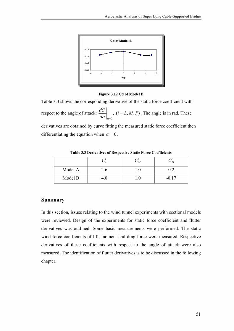
Aeroelastic Analysis of Super Long Cable-Supported Bridge
51
Cd of Model B
0.00
0.05
0.10
0.15
-6 -4 -2 0 2 4 6
deg
Figure 3.12 Cd of Model B
Table 3.3 shows the corresponding derivative of the static force coefficient with
respect to the angle of attack: 0=ααd
dCi , ),,( PMLi = . The angle is in rad. These
derivatives are obtained by curve fitting the measured static force coefficient then
differentiating the equation when 0=α .
Table 3.3 Derivatives of Respective Static Force Coefficients
LC ′ MC ′ DC ′
Model A 2.6 1.0 0.2
Model B 4.0 1.0 -0.17
Summary In this section, issues relating to the wind tunnel experiments with sectional models
were reviewed. Design of the experiments for static force coefficient and flutter
derivatives was outlined. Some basic measurements were performed. The static
wind force coefficients of lift, moment and drag force were measured. Respective
derivatives of these coefficients with respect to the angle of attack were also
measured. The identification of flutter derivatives is to be discussed in the following
chapter.
Aeroelastic Analysis of Super Long Cable-Supported Bridge
52
CHAPTER FOUR
Method Used To Identify Flutter Derivatives
Abstract
Many identification methods have been used effectively to extract flutter derivatives.
In this section, the method of ERA (eigensystem realization algorithm) is reviewed
and selected as the tool to do the identification. The flutter derivative model is a
linear equation with reduced frequency dependent parameters. In the experiment, at
each wind speed level, it reduces to a linear equation with constant coefficients
corresponding to specified reduced frequency. It suffices to identify it as a time-
invariant linear dynamic system.
Aeroelastic Analysis of Super Long Cable-Supported Bridge
53
4.1 Introduction
Many methods have been tried for the identification of flutter derivatives.
Shinozuka (1982) used ARMA models to identify flutter derivatives. Yamada et al.
(1992) used the extended Kalman filter method to retrieve the aforementioned
parameters from coupled vibration time histories. Bogunovic-Jakobsen (1995)
followed Hoen (1991, 1993) to employ ambient response to recover covariance
function estimates for the identification of aeroelastic derivatives. There are many
other exercises not mentioned. In this work, the last mentioned method is followed.
The essence of this method is to employ the classic idea in stochastic identification
of using output covariance as Markov parameters, which was further used in
Eigensystem Realization Algorithm (ERA).
ERA is a minimum order realization method. Although for experiments with
sectional model, the number of degrees of freedom is known beforehand and there
is no need to determine the system order in the sense of minimum state-space
dimensions, this method offers us a good framework to discuss the errors in the
identification through singular-values.
4.2 Basics of ERA
In this part, the method of ERA is reviewed after a short introduction of the
historical development of the method.
4.2.1 The History of ERA
It is common to construct state-space representation of linear systems. Gilbert
(1963) and Kalman (1963) introduce the important principles of realization theory
in terms of the concepts of controllability and observability. Ho and Kalman (1966)
showed that the minimum realization problem is equivalent to a representation
Aeroelastic Analysis of Super Long Cable-Supported Bridge
54
problem involving a sequence of real matrices known as Markov Parameters (pulse
response function). By minimum realization is meant a model with the smallest
state-space dimension among systems realized that have the same input-output
relations within a specified degree of accuracy.
A common weakness of the schemes of that time is that the effects of noise on the
data analysis were not evaluated. Zeiger and McEwen (1974) proposed a
combination of the Ho-Kalman algorithm with the singular–value decomposition
technique for the treatment of noisy data. However, no theoretical or numerical
studies were reported by them. The singular-value decomposition technique has
been widely recognized as being very effective and numerically stable. It was used
by Juang and Pappa (1984) to form ERA for modal parameter identification of
flexible structures.
ERA consists of two major parts, namely, basic formulation of minimum-order
realization and modal parameter realization. In the first part, the Hankel matrix,
which represents the data structure for the Ho-Kalman algorithm, is generalized to
allow random distribution of Markov parameters generated by free decay response.
Then Ho-Kalman algorithm is combined with singular-value decomposition to
identify the dynamic system. In modal space, modal parameters are identified.
4.2.2 The Method of ERA
(Juang and Pappa, 1984, 1986; Juang 1994)
Linear dynamic systems can be expressed in the form of state equations. The
collection of state variables in state equations is the state of the system. The set of
all possible states is the state space of the system.
Rewriting the system equation of a bridge deck
)(tpxKxCxM effeff =++ &&& (4.2.1)

Aeroelastic Analysis of Super Long Cable-Supported Bridge
55
in state equation form, with input )(tp , output Tphx α,,= , we have,
)(tpBXAX cc +=& (4.2.2)
)(tDvCXY += (4.2.3)
with state matrix
−−
= −−effeff
c CMKMI
A 11
0, (4.2.4)
input matrix
= −1
0M
Bc , (4.2.5)
output matrix C , feed through matrix D and state variable TTT xxX &,= .
For bridge deck experiments, C= [ ]0I and D is zero.
The discrete time state space equation of the same systems above is in the form:
)()()1( iBpiAXiX +=+ (4.2.6)
)()( iCXiY = (4.2.7)
Where tAceA ∆= (4.2.8)
and
∫∆
=t
cA dBeB c
0ττ (4.2.9)
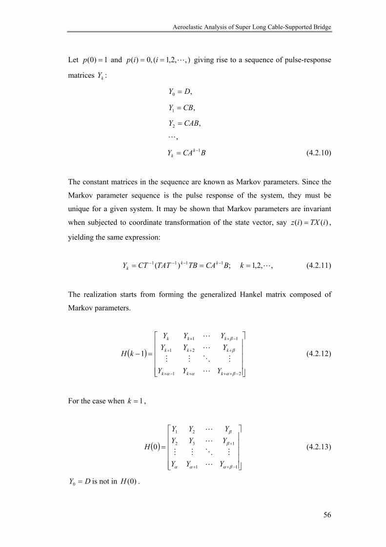
Aeroelastic Analysis of Super Long Cable-Supported Bridge
56
Let 1)0( =p and ),,2,1(,0)( L== iip giving rise to a sequence of pulse-response
matrices kY :
,0 DY =
,1 CBY =
,2 CABY =
,L
BCAY kk
1−= (4.2.10)
The constant matrices in the sequence are known as Markov parameters. Since the
Markov parameter sequence is the pulse response of the system, they must be
unique for a given system. It may be shown that Markov parameters are invariant
when subjected to coordinate transformation of the state vector, say )()( iTXiz = ,
yielding the same expression:
,,2,1;)( 1111 L=== −−−− kBCATBTATCTY kkk (4.2.11)
The realization starts from forming the generalized Hankel matrix composed of
Markov parameters.
( )
=−
−+++−+
+++
−++
21
21
11
1
βααα
β
β
kkk
kkk
kkk
YYY
YYYYYY
kH
L
MOMM
L
L
(4.2.12)
For the case when 1=k ,
( )
=
−++
+
11
132
21
0
βααα
β
β
YYY
YYYYYY
H
L
MOMM
L
L
(4.2.13)
DY =0 is not in )0(H .
Aeroelastic Analysis of Super Long Cable-Supported Bridge
57
If nn >> βα , ( n is the order of the state-space model), the matrix )(kH is of rank
n . To confirm this we can decompose )(kH into three matrices
βα QAPkH k=)( (4.2.14)
Where block matrix αP is the observability matrix:
=
−1
2
α
α
CA
CACAC
PM
(4.2.15)
and βQ is the controllability matrix:
[ ]BABAABBQ 12 −= ββ L (4.2.16)
If the system is controllable and observable, αP and βQ are of rank n . Therefore
nkHr =))(( . (4.2.17)
If the first Block Hankel matrix )0(H is factored by singular value decomposition
(SVD): TSRH Σ=)0( (4.2.18)
where the columns of R and S are orthonormal and Σ is a rectangular matrix
Σ=Σ
000n (4.2.19)
with
Aeroelastic Analysis of Super Long Cable-Supported Bridge
58
[ ]nn diag σσσ L21=Σ (4.2.20)
having diagonal elements monotonically non-increasing, i.e.
nσσσ ≥≥≥ L21 . (4.2.21)
Hence the number of non zero singular values n equals the rank of )0(H .
If R and TS are partitioned as
][ 0RRR n= and ][ 0TT
nT SSS = , (4.2.22)
observation on the expression suggests that matrices αP and βQ are related to R
and TS , respectively. Indeed,
2/1
nnRP Σ=α (4.2.23)
T
n SQ 2/1Σ=β (4.2.24)
In reality, the Block Hankel Matrix will always be full rank due to noise
components in the signal, non-linearity or computation round-off. However the
singular-value decomposition technique has been widely recognized as being very
effective and numerically stable in that small perturbations in the matrix generate
small perturbations in Σ . Some of the singular-values, inn σσσ ,,, 21 L++ may be
small and negligible in the sense that they contain more noise information than
system information. It is equivalent to saying that the directions determined by them
have less significant degrees of controllability and observability relative to the
noise. In this case, we should assume that:
βα QAPkH k≈)( (4.2.25)
Specifically,
Aeroelastic Analysis of Super Long Cable-Supported Bridge
59
βαQPH ≈)0( (4.2.26)
If the noise component in the Hankel Matrix is not too big, the solution should be
still acceptable. Therefore we have
T
nnn SARAQPH 2/12/1)1( ΣΣ== βα . (4.2.27)
Therefore 2/12/1* )1( −− ΣΣ= n
Tn
Tnn SHRA (4.2.28)
Tnn SB 2/1* Σ= (4.2.29)
2/1*
nnRC Σ= (4.2.30)
Where ' * ' denotes similar transformation of respective matrix, since it is known
that the identified result is the same with respect to similar transformation. In the
experiments to extract aeroelastic derivatives, all the degrees of freedom are
measured; it is possible to transform the identified result back to observability
canonical form.
Because it is possible to ensure in the experiment that the output matrix is
]0[IC = (4.2.31)
for the observability canonical realization, the observability matrix is equal to the
identity matrix, i.e.
ICAC
Q =
= (4.2.32)
Under the nonsingular transform,

Aeroelastic Analysis of Super Long Cable-Supported Bridge
60
*TXX = (4.2.33)
where T is a nonsingular transform matrix. Applying this in the state-space
equation,
)()()1( 1*1* iBpTiATXTiX −− +=+ (4.2.34)
)()( * iCTXiY = (4.2.35)
the identified observability matrix can be expressed as
TQTATCTT
CTAC
CQ ==
=
= −1**
** (4.2.36)
So, we have the original discrete time state matrix, output and input matrices as:
1* −= TTAA (4.2.37)
*TBB = (4.2.38)
1* −= TCC (4.2.39)
The method of ERA is completed.
Summary
In this section, system identification methods for the identification of flutter
derivatives were reviewed. ERA is the method to be used in the study.

Aeroelastic Analysis of Super Long Cable-Supported Bridge
61
CHAPTER FIVE
Effect of Relative Amplitude and Lateral Aerodynamic Derivatives on Bridge Deck Flutter I:
Experimental Detection of Nonlinearity in Self-Excited Forces
Abstract:
The self-excited wind forces on a bridge deck can be nonlinear even when the
vibration amplitude of the body is small. In this chapter, experiments detecting the
nonlinearity are described with the concept of “relative amplitude”, i.e. the
amplitude of the externally triggered free vibration relative to the envelope of the
ambient response of an elastically supported rigid sectional model. The effect of
relative amplitude on flutter derivatives and on the flutter boundary reveals, from
the structural point of view, a complex relationship between the self-excited forces
and the “structural vibration noise” due to signature turbulence related buffeting
forces. Although the aeroelastic forces are linear when the body motion due to an
external trigger is not affected significantly by the signature turbulence, they are
nonlinear when the noise component in the vibration due to the signature
turbulence related buffeting forces cannot be neglected. Two and three-dimensional
wind tunnel experiments with two types of sectional models were performed to
detect the existence of nonlinearity in the interactive wind forces.
Aeroelastic Analysis of Super Long Cable-Supported Bridge
62
5.1 Introduction:
This research studies the characteristics of interactive wind forces on bridge decks
at flutter.
Under the action of net wind forces on the bridge, the structure may deflect, causing
it as a whole to respond in its natural vibration modes. Some prominent modes may
attract interactive aerodynamic forces that lead to modal auto-excitation. In this
situation, the strong linear tendencies of a large elastic structure actually
predominate, permitting a simplified linear appreciation of what is indeed a highly
complex nonlinear phenomenon at least insofar as detailed loading is concerned. By
employing a flutter derivative model, a linearized representation of the self-excited
wind loads is obtained.
Previous researches (Scanlan 1997, Falco et al 1992) have indicated amplitude
dependency of the measured flutter derivatives. From this point of view,
nonlinearity does not exist for the small amplitude analysis. As a matter of fact, the
self-excited wind force due to a pulse input can be nonlinear even if the response
amplitude is small.
To illustrate this, it is necessary to include another issue: turbulence effects on
flutter derivatives and, further, on the flutter instability. As criticized by Cai et al
(1999), many theoretical and experimental studies of flutter were conducted in
smooth flow (Scanlan 1978a, 1978b; Namini 1989) for the reason of avoiding both
mathematical complexity and technical difficulty. Scanlan and Jones (1990) and
Jain et al. (1996) argued the effect of turbulence could be reflected by testing the
flutter derivatives under suitable conditions of turbulence and incorporating the
span-wise coherence effect of flutter derivatives into the formulation. By
recognition of a span-wise diminution of coherence in the associated flutter
derivatives, a higher critical wind speed for flutter is usually expected. The
argument is supported by experimental observations in wind tunnel. Typically, as
has been observed repeatedly, an extended span bridge model in the wind tunnel

Aeroelastic Analysis of Super Long Cable-Supported Bridge
63
becomes unstable at a certain crosswind velocity under smooth approaching flow
but at a distinctly higher one under turbulent flow (Scanlan 1997).
Lin and Li (1993, 1995) followed by Cai et al. (1999a) introduced the stochastic
method for predicting instability of wind-excited structures, making it possible to
consider the self-excited forces as random values to model the random nature of
turbulent wind. Flutter derivatives in smooth flow are used. The self-excited forces
are presented as a function of fluctuating wind speed.
The major problem of the methods, however, is that they do not carry the
information that the existence of buffeting response may change the feature of the
interactive forces and flutter derivatives, as will be shown in this chapter. A set of
flutter derivatives identified for flutter instability analysis may not be suitable for
the analysis when effects of buffeting forces are being considered. The argument of
a span-wise diminution of coherence in the associated flutter derivatives (Scanlan
1997) is a supplement for the free decay vibration testing in turbulent flow. Studies
(Sarkar et al 1994) have shown that turbulence effect on the measured flutter
derivatives is not noticeable. However, the tests were based on free decay vibration
testing. The tests with free decay or forced sinusoidal motion usually deal with a
clear harmonic motion, even if the turbulence is included. This situation, however,
exaggerates the effect of structural motion by forcing the surrounding fluid to
behave in phase with the body, increasing the span-wise coherence of the flutter
derivatives. If the magnitude of the pulse response of the rigid model is reduced to a
smaller level, i.e. within the ambient response vibration envelope, so that the
ambient response property of the aeroelastic system can be preserved, the effect of
turbulence on flutter derivatives will be manifested. This is a condition under which
more information from the fluid may be obtained.
5.2 The Relative Amplitude Effect
To investigate the nonlinearity in the self-excited wind forces, we shall limit our
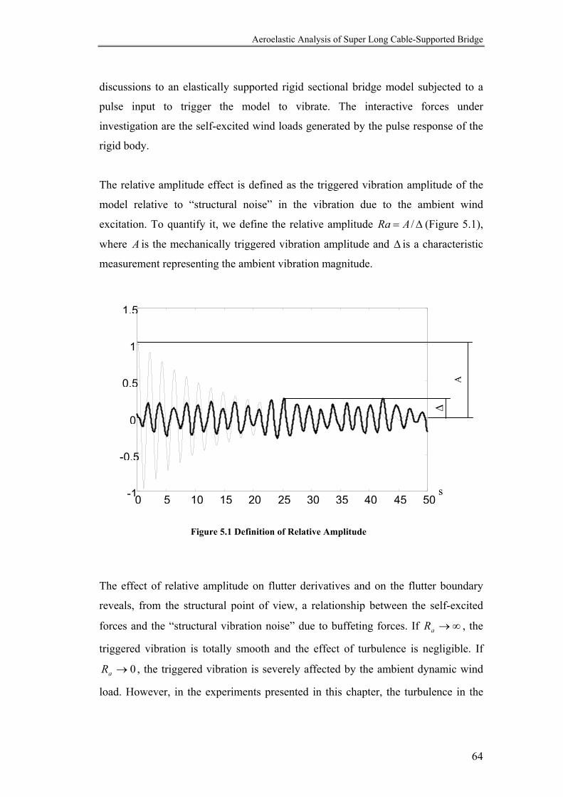
Aeroelastic Analysis of Super Long Cable-Supported Bridge
64
discussions to an elastically supported rigid sectional bridge model subjected to a
pulse input to trigger the model to vibrate. The interactive forces under
investigation are the self-excited wind loads generated by the pulse response of the
rigid body.
The relative amplitude effect is defined as the triggered vibration amplitude of the
model relative to “structural noise” in the vibration due to the ambient wind
excitation. To quantify it, we define the relative amplitude ∆= /ARa (Figure 5.1),
where A is the mechanically triggered vibration amplitude and ∆ is a characteristic
measurement representing the ambient vibration magnitude.
The effect of relative amplitude on flutter derivatives and on the flutter boundary
reveals, from the structural point of view, a relationship between the self-excited
forces and the “structural vibration noise” due to buffeting forces. If ∞→aR , the
triggered vibration is totally smooth and the effect of turbulence is negligible. If
0→aR , the triggered vibration is severely affected by the ambient dynamic wind
load. However, in the experiments presented in this chapter, the turbulence in the
0 5 10 15 20 25 30 35 40 45 50-1
-0.5
0
0.5
1
1.5
∆
A
s
Figure 5.1 Definition of Relative Amplitude

Aeroelastic Analysis of Super Long Cable-Supported Bridge
65
oncoming flow was not generated artificially due to the limitations of equipment.
The buffeting response in the following experiment is mainly due to the signature
turbulence and turbulence in the approaching flow (turbulence intensity was less the
2% during the experiment, Table 3.1).
5.3 Physical Significance of Flutter Derivatives with Different
Relative Amplitudes
Discussions in the previous section may be summarized from another point of view.
We also limit our discussions to the interactive force on an elastically supported
rigid sectional bridge model due to a pulse response. In the wind tunnel experiment,
the sectional model is always responding to the ambient wind excitation, namely the
turbulence in the oncoming flow, and the signature turbulence generated by the
bluff structure itself when wind is passing by. This ambient response forms the
“environment” for the impulse response to exist. It could be a different story if the
pulse response of the sectional model is strong and destroys the ambient response,
or the pulse response is small with all the “ambient properties” of the aeroelastic
system unchanged.
The difference will be told by the various flutter derivatives identified with different
relative amplitudes. Experiments will show whether or not the turbulence effect
will manifest itself when the relative amplitude is small and causes nonlinearity in
the self-excited force.
For a flexible bridge in the wind, if there is no relative amplitude effect considered,
usually, the flutter analysis predicts the critical wind speed for a smooth sustained
sinusoidal motion of the deck, which indicates the bridge is going to lose its
stability due to negative damping. However, a “smooth” sinusoidal motion is rarely
the real case when there are disturbances in the aerodynamic forces. The ambient
vibration exists. An initially small amplitude sinusoidal motion can be only
Aeroelastic Analysis of Super Long Cable-Supported Bridge
66
considered as a “noisy” sinusoidal motion. It needs to be answered in the first place
whether or not the noisy sinusoidal motion will grow in the “environmental noise1”
and become larger in amplitude making itself smoother (the ambient vibration then
becomes relatively unimportant) before a flutter prediction is applied.
Based on this understanding, in reference to the frequency domain method to
predict the flutter boundary (Jain et al. 1996), there should be two thresholds AmbU
and TranU of the wind speed. The former is for a signal to diverge in the context of
ambient response, the latter is for a large amplitude signal to diverge after going
outside “ambient vibration envelope”. If a signal cannot diverge in the former case,
i.e. AmbUU < , it would not go to the stage of latter case. Theoretically, it is stable to
wind excitation. If the signal diverges from ambient response to larger amplitude
but subsequently decays, i.e. TranAmb UUU << , the response is bounded. If the
signal diverges in both cases, i.e. UU Amb < & UUTran < , the system is not stable.
It is interesting to consider the case where AmbTran UU < . Under this condition, the
judgment of the onset of flutter based on AmbU is not safe, since there could be other
sources of excitation contributing to the dynamic response. A strong gust, for
example, could push the bridge deck outside the normal ambient vibration
envelope. After the gust, the bridge deck may decay back from outside into the
ambient vibration envelope. Before the gust, the critical wind speed for flutter is
ambU , after the gust, however, the critical wind speed may change to tranU , which
may be lower than ambU . This is shown in Figure 5.2. If flutter happens in this way,
a transient rather than steady critical flutter wind speed exists. It will be
conservative to use TranU as the design flutter wind speed in this case.
1 This response is termed “noise” instead of buffeting response because the buffeting response of the flexible prototype carries many modes of different frequencies, which may be very difficult, if not impossible, to be reflected by sectional model testing. The discussion in this research is limited to the effect of “noise”. No special spectrum of it will be considered.

Aeroelastic Analysis of Super Long Cable-Supported Bridge
67
5.4 Use Of Output Covariance As Markov Parameters
It is difficult, if not impossible, to identify the flutter derivatives when the pulse
response is small in amplitude compared with the ambient vibration. However a
pulse response or Markov Parameters, if the discrete form is considered, can be
produced mathematically by using output covariance of ambient vibration. (Hoen et al
1993, Jakobsen and Hansen 1995). This corresponds to the extreme case where the
pulse response amplitude tends to zero.
The input term, buffeting force on the bridge deck model, is random and unknown
and assumed to be white noise. We assume the displacement measurement is zero
mean. If the deck has a static displacement due to the static wind load, it can be
treated as centered process, i.e.
[ ])()()( tYEtYtY −= (5.5.1)
where [ ]•E denotes expectation operation.
Therefore, we always assume we are dealing with a zero mean process.
As mentioned in Chapter 4, it is a classical result in stochastic identification that the
output covariance can be used as Markov parameters of deterministic linear time
invariant system when the measurement noise in the equipment and process noise
U
t
U amb Utran
Figure 5.2 Non-Stationary Flutter Boundary
Aeroelastic Analysis of Super Long Cable-Supported Bridge
68
(the small scale buffeting force due to signature turbulence and local variation of
wind speed in the oncoming flow) is white and zero mean. Markov parameters are
the discrete version of pulse response function; a proof is presented in the Appendix
I. The output covariance produces a new discrete state-space model of
)0(,,, iCCGA , where A is the state matrix; G is the input matrix;C is the output
matrix and )0(iC is the initial condition. Matrix G and )0(iC are defined in the
Appendix I.
One consideration is that within the time period of measurement of the ambient
vibration, the system is actually non-stationary due to uncontrollable experimental
conditions. Therefore, in calculating the output covariance, some numerical
consideration has been taken to overcome the problem, which will be addressed in
the following section.
5.5 Numerical Considerations for Computation of Output
Covariance
The structure function was introduced by Kolmogorov (1941) in his study of locally
isotropic and homogeneous stochastic turbulence. It is defined as:
[ ] ))()0((2)()(1lim)(
0
2 τττ tt
T
TCCdttYtY
TZ −=+−= ∫
∞→ (5.5.1)
where )(τtC is the auto-covariance function of the measurement after time τ+t .
For ambient vibration, the covariance function for zero lag time is constant, and the
structure function is the sum of the negative covariance function and a constant. If
the measurement shows slow fluctuation or has a time varying trend, i.e. shows
marked derivation from a stationary behavior, the method of structure function may
be advantageous because the structure function can tolerate more low frequency
noise than the correlation function (Solnes 1997).
Consider, for example, a simple harmonic function ttx ωsin)( = without random
Aeroelastic Analysis of Super Long Cable-Supported Bridge
69
amplitude and phase, the process can be shown to have an autocorrelation
function ttRx ωcos21)( = , by taking care to integrate over an integer number of half
circles πω nT = . Since this condition is almost impossible to realize in practice,
systematic error is introduced. Near the origin, 1<ωτ , the limit of error can be
shown as:
TTRx ω
ωτ2
)2sin(21)( −≈∆ . (5.5.2)
For the auto-structural function, the limit of error is
TTZ x ω
ωτωτ2
)2sin(21)( 22−≈∆ . (5.5.3)
This shows that the structural function is less distorted for 1<ωτ , hence is less
susceptible to low-frequency noise.
5.6 The Experiment
The two sectional models A & B described in Chapter 3 were tested. For the bluff
twin deck model A, two-dimensional ambient and transient vibration experiments
were carried out. For the partially streamlined box girder model B, both two and
three-dimensional tests were done with transient and ambient vibration. Transient
and ambient vibrations were recorded under the same condition. No turbulence in
the oncoming flow was artificially generated. The procedures were outlined in
previous chapters. In all of the experiments the signal outputs from the laser
displacement sensor and anemometer were recorded at 200Hz sampling rate.
System identification procedure was then applied. The method used was ERA
(eigensystem realization algorithm) as described in Chapter 4. After the state
matrices A and cA were recovered, the aeroelastic system parameters were
converted to flutter derivatives, the conversion is given in Chapter 3.
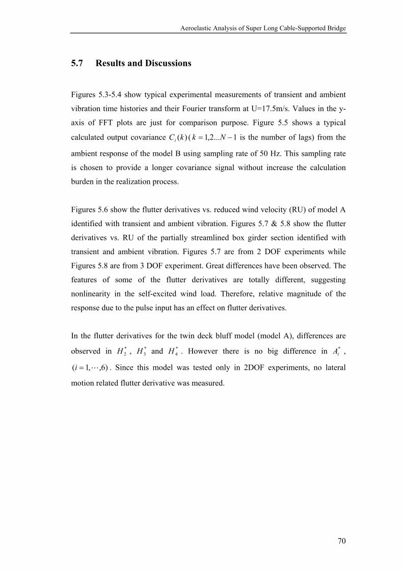
Aeroelastic Analysis of Super Long Cable-Supported Bridge
70
5.7 Results and Discussions
Figures 5.3-5.4 show typical experimental measurements of transient and ambient
vibration time histories and their Fourier transform at U=17.5m/s. Values in the y-
axis of FFT plots are just for comparison purpose. Figure 5.5 shows a typical
calculated output covariance )(kCi ( 1...2,1 −= Nk is the number of lags) from the
ambient response of the model B using sampling rate of 50 Hz. This sampling rate
is chosen to provide a longer covariance signal without increase the calculation
burden in the realization process.
Figures 5.6 show the flutter derivatives vs. reduced wind velocity (RU) of model A
identified with transient and ambient vibration. Figures 5.7 & 5.8 show the flutter
derivatives vs. RU of the partially streamlined box girder section identified with
transient and ambient vibration. Figures 5.7 are from 2 DOF experiments while
Figures 5.8 are from 3 DOF experiment. Great differences have been observed. The
features of some of the flutter derivatives are totally different, suggesting
nonlinearity in the self-excited wind load. Therefore, relative magnitude of the
response due to the pulse input has an effect on flutter derivatives.
In the flutter derivatives for the twin deck bluff model (model A), differences are
observed in *2H , *
3H and *4H . However there is no big difference in *
iA ,
)6,,1( L=i . Since this model was tested only in 2DOF experiments, no lateral
motion related flutter derivative was measured.
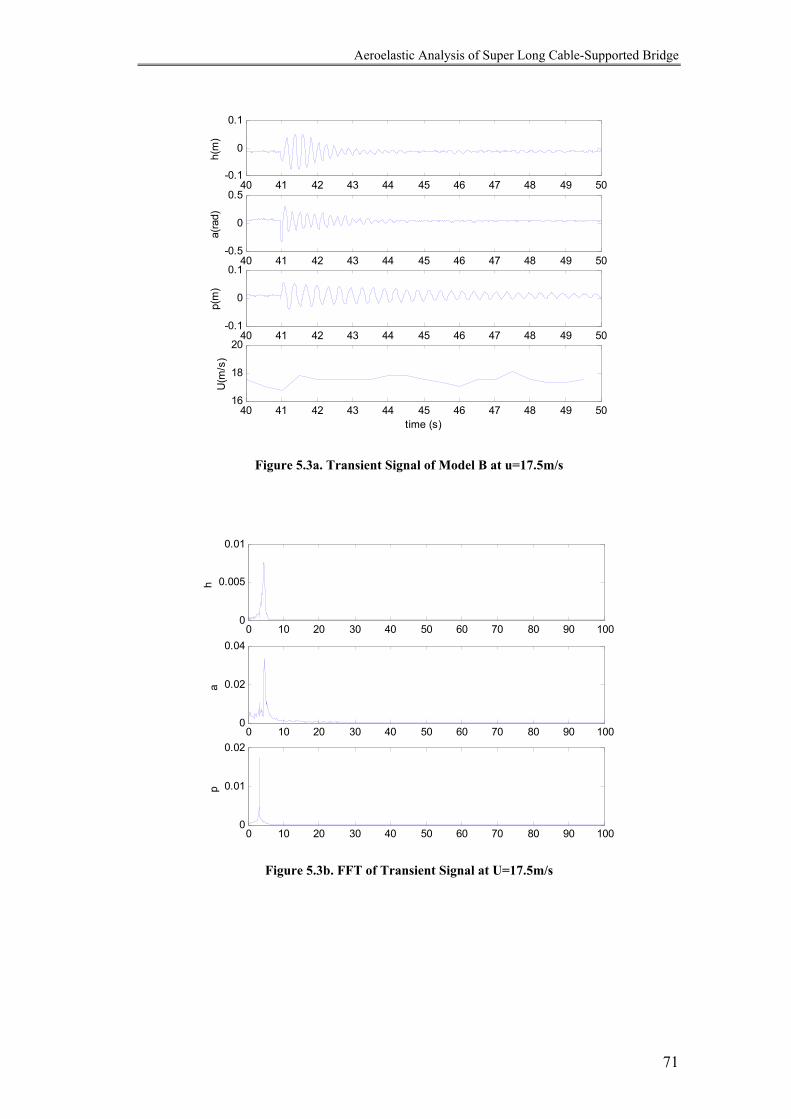
Aeroelastic Analysis of Super Long Cable-Supported Bridge
71
40 41 42 43 44 45 46 47 48 49 50-0.1
0
0.1
h(m
)
40 41 42 43 44 45 46 47 48 49 50-0.5
0
0.5
a(ra
d)
40 41 42 43 44 45 46 47 48 49 50-0.1
0
0.1
time (s)
p(m
)
40 41 42 43 44 45 46 47 48 49 5016
18
20
time (s)
U(m
/s)
Figure 5.3a. Transient Signal of Model B at u=17.5m/s
0 10 20 30 40 50 60 70 80 90 1000
0.005
0.01
h
0 10 20 30 40 50 60 70 80 90 1000
0.02
0.04
a
0 10 20 30 40 50 60 70 80 90 1000
0.01
0.02
p
Figure 5.3b. FFT of Transient Signal at U=17.5m/s
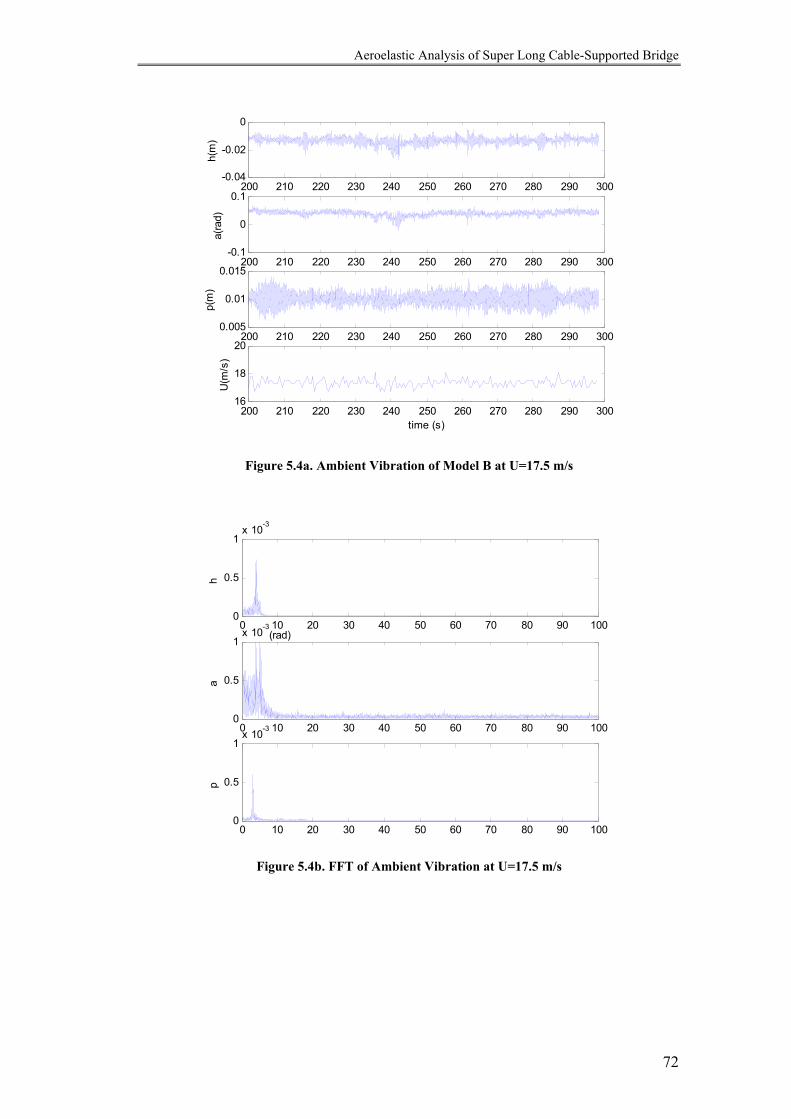
Aeroelastic Analysis of Super Long Cable-Supported Bridge
72
200 210 220 230 240 250 260 270 280 290 300-0.04
-0.02
0
h(m
)
200 210 220 230 240 250 260 270 280 290 300-0.1
0
0.1
a(ra
d)
200 210 220 230 240 250 260 270 280 290 3000.005
0.01
0.015
time (s)
p(m
)
200 210 220 230 240 250 260 270 280 290 30016
18
20
time (s)
U(m
/s)
Figure 5.4a. Ambient Vibration of Model B at U=17.5 m/s
0 10 20 30 40 50 60 70 80 90 1000
0.5
1x 10⁻³
h
0 10 20 30 40 50 60 70 80 90 1000
0.5
1x 10⁻³
a
0 10 20 30 40 50 60 70 80 90 1000
0.5
1x 10⁻³
p
(rad)
Figure 5.4b. FFT of Ambient Vibration at U=17.5 m/s
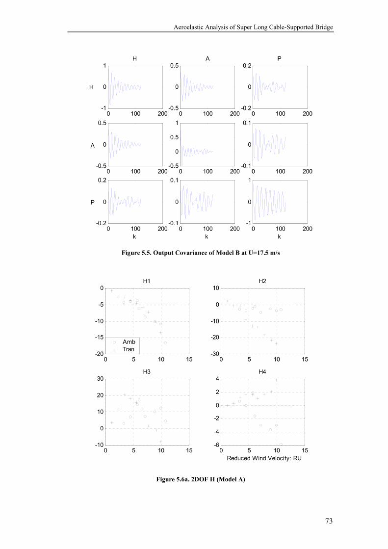
Aeroelastic Analysis of Super Long Cable-Supported Bridge
73
0 100 200-1
0
1H
0 100 200-0.5
0
0.5
0 100 200-0.2
0
0.2P
0 100 200-0.5
0
0.5
0 100 200-0.5
0
0.5
1
0 100 200-0.1
0
0.1
0 100 200-0.2
0
0.2
k0 100 200
-0.1
0
0.1
k0 100 200
-1
0
1
k
A
H
A
P
Figure 5.5. Output Covariance of Model B at U=17.5 m/s
0 5 10 15-20
-15
-10
-5
0H1
Amb Tran
0 5 10 15-30
-20
-10
0
10H2
0 5 10 15-10
0
10
20
30H3
0 5 10 15-6
-4
-2
0
2
4H4
Reduced Wind Velocity: RU
Figure 5.6a. 2DOF H (Model A)

Aeroelastic Analysis of Super Long Cable-Supported Bridge
74
0 5 10-1.5
-1
-0.5
0
0.5A1
0 5 10-1
-0.8
-0.6
-0.4
-0.2
0A2
0 5 10-0.5
0
0.5
1
1.5
2A3
0 5 10-0.4
-0.2
0
0.2
0.4A4
Reduced Wind Velocity: RU
Amb Tran
Figure 5.6b. 2DOF A (Model A)
0 5 10 15-10
-5
0
5H1
0 5 10 15-60
-40
-20
0
20
40H2
0 5 10 15-50
0
50
100
150H3
0 5 10 15-20
-10
0
10
20H4
Reduced Wind Velocity: RU
Amb Tran
Figure 5.7a. 2DOF H (Model B)

Aeroelastic Analysis of Super Long Cable-Supported Bridge
75
0 5 10 15-1.5
-1
-0.5
0
0.5A1
0 5 10 15-2
-1.5
-1
-0.5
0
0.5A2
0 5 10 15-1
0
1
2A3
0 5 10 15-1
-0.5
0
0.5A4
Reduced Wind Velocity: RU
Amb Tran
Figure 5.7b. 2DOF A (Model B)
0 10 20-15
-10
-5
0
5H1
0 10 20-60
-40
-20
0
20
40H2
0 10 20-50
0
50
100
150
200H3
0 10 20-15
-10
-5
0
5
10H4
0 10 20-10
-5
0
5
10H5
0 10 20-20
-10
0
10
20H6
Reduced Wind Velocity: RU
Amb Tran
Figure 5.8a. 3DOF H (Model B)
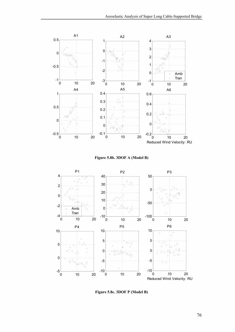
Aeroelastic Analysis of Super Long Cable-Supported Bridge
76
0 10 20-1
-0.5
0
0.5A1
0 10 20-3
-2
-1
0
1A2
0 10 20-1
0
1
2
3
4A3
0 10 20-0.5
0
0.5
1A4
0 10 20-0.1
0
0.1
0.2
0.3
0.4A5
0 10 20-0.2
0
0.2
0.4
0.6A6
Reduced Wind Velocity: RU
Amb Tran
Figure 5.8b. 3DOF A (Model B)
0 10 20-4
-2
0
2
4P1
0 10 20-10
0
10
20
30
40P2
0 10 20-100
-50
0
50P3
0 10 20-5
0
5
10P4
0 10 20-10
-5
0
5
10P5
0 10 20-10
-5
0
5
10P6
Reduced Wind Velocity: RU
Amb Tran
Figure 5.8c. 3DOF P (Model B)
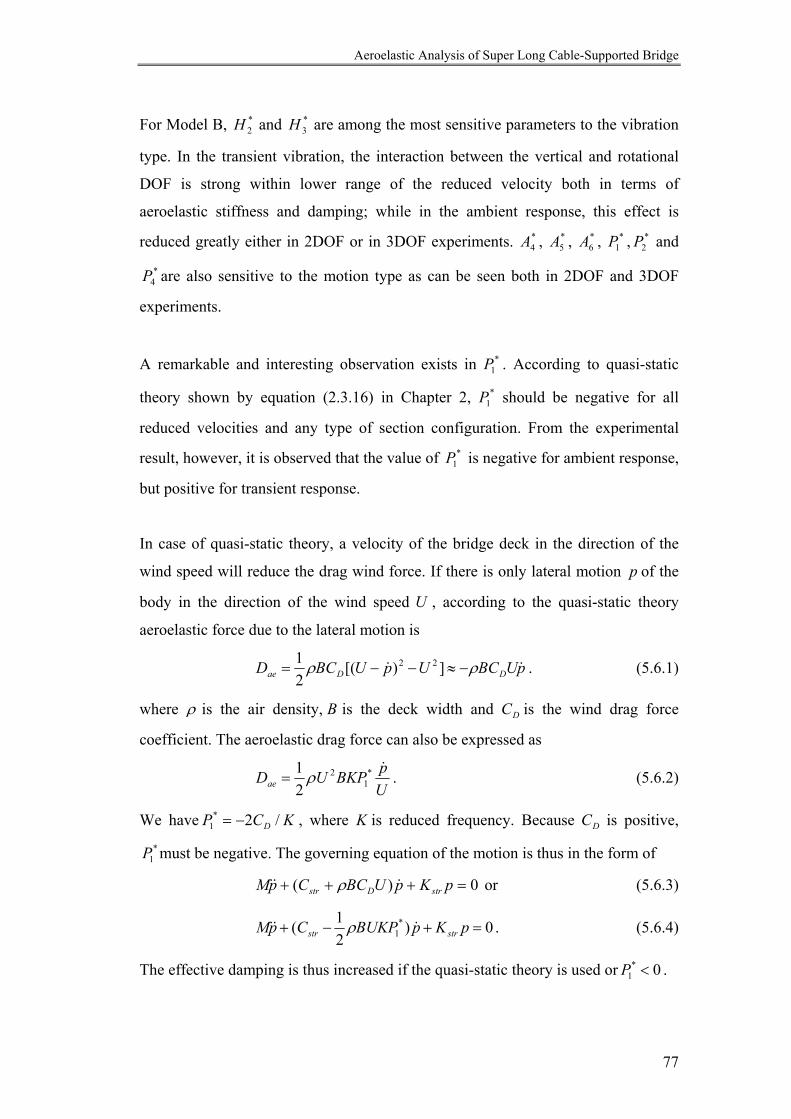
Aeroelastic Analysis of Super Long Cable-Supported Bridge
77
For Model B, *2H and *
3H are among the most sensitive parameters to the vibration
type. In the transient vibration, the interaction between the vertical and rotational
DOF is strong within lower range of the reduced velocity both in terms of
aeroelastic stiffness and damping; while in the ambient response, this effect is
reduced greatly either in 2DOF or in 3DOF experiments. *4A , *
5A , *6A , *
1P , *2P and
*4P are also sensitive to the motion type as can be seen both in 2DOF and 3DOF
experiments.
A remarkable and interesting observation exists in *1P . According to quasi-static
theory shown by equation (2.3.16) in Chapter 2, *1P should be negative for all
reduced velocities and any type of section configuration. From the experimental
result, however, it is observed that the value of *1P is negative for ambient response,
but positive for transient response.
In case of quasi-static theory, a velocity of the bridge deck in the direction of the
wind speed will reduce the drag wind force. If there is only lateral motion p of the
body in the direction of the wind speed U , according to the quasi-static theory
aeroelastic force due to the lateral motion is
pUBCUpUBCD DDae && ρρ −≈−−= ])[(21 22 . (5.6.1)
where ρ is the air density, B is the deck width and DC is the wind drag force
coefficient. The aeroelastic drag force can also be expressed as
UpBKPUDae&*
12
21 ρ= . (5.6.2)
We have KCP D /2*1 −= , where K is reduced frequency. Because DC is positive,
*1P must be negative. The governing equation of the motion is thus in the form of
0)( =+++ pKpUBCCpM strDstr &&& ρ or (5.6.3)
0)21( *
1 =+−+ pKpBUKPCpM strstr &&& ρ . (5.6.4)
The effective damping is thus increased if the quasi-static theory is used or 0*1 <P .
Aeroelastic Analysis of Super Long Cable-Supported Bridge
78
However, the quasi-static theory is recognized to be only a nominal form that may
hold for very slow changes in the angle of attack and wind speed. It is, strictly
speaking, asymptotic case approached at high-reduced velocity e.g. the case when
vibration frequency 0→n and the reduced velocity ∞→= nBURU / .
For the triggered 3DOF experiment, however, the acceleration in the lateral
direction is the major reason for the generation of aerodynamic damping. Lin and
Yang (1983) suggested impulse response functions of the self-excited force due,
separately, to velocity and acceleration of the rigid body. By using Duhammel
integral, the acceleration related effect will become velocity related, i.e. added
damping effect. In this case, it is hard to say that the *1P must be negative because
the acceleration can be either positive or negative for a given velocity in the quasi-
static expressions. The time domain SEF model, which will be shown in Chapter 7
of this thesis, also points to the same conclusion: a velocity in the direction of wind
speed could increase the drag force. This may indicate that omitting the derivatives *
iP )6,,1( L=i may not be always safe for the prediction of the flutter boundary.
In the ambient response, the bridge deck model is driven by noise instead of a non-
zero initial condition as is in the transient vibration. The coherence of the interactive
fluid behavior along the axis of the model might be smaller in the former case than
in the later case. This is observed in the reduction in values of some of flutter
derivatives as *2H and *
3H , but not necessarily for others such as *1P and *
4P .
Transient vibration and ambient response represent the two cases where the
structural noise component accounts for a small part of the total signal energy and
100 percent of it, respectively. In the former case, the effect of initial condition is
the main factor of the experiment; while in the later case, the effect of the
“structural vibration noise” is exaggerated. The relative amplitude effect, i.e. the
significance of the consequence of the model being bluff in affecting the interactive
forces, is thus studied. The comparison of these two extreme conditions reveals that
the function of flutter derivatives of a particular section depends not only on
reduced velocity or reduced frequency but also relative amplitude of the vibration.

Aeroelastic Analysis of Super Long Cable-Supported Bridge
79
In transient vibration tests, the triggered vibration is clearly larger than the ambient
vibration when it starts, but decays very fast into the ambient vibration envelope. At
the beginning, the relative amplitude effect is negligible, but it is not at the end. The
identification of flutter derivatives corresponding to the free decay vibration
actually deals with a time-varying phenomenon if the vibration decays very fast. On
the contrary, in the experiment with ambient vibration, there is no change in the
relative amplitude because the pulse response is calculated numerically by output
covariance. The phenomenon to be identified is time-invariant under this condition.
As will be shown in the later chapter, the linear identification can approximate the
output covariance of the ambient response better than the triggered transient
vibration. This may support the idea that the relative amplitude effect on flutter
derivatives is not negligible.
Summary
In this study, nonlinearity in self-excited wind forces is detected through the
concept of relative amplitude effect. By comparing the flutter derivatives identified
from triggered free decay and ambient vibration of the elastically supported rigid
sectional bridge model, the relative amplitude effect on the interactive wind forces
is manifested. This effect, from the structural point of view, reveals a complex
relationship between the self-excited forces and the “structural vibration noise” due
to ambient wind excitations. Although the aeroelastic forces are linear when the
body motion due to an external trigger is not affected significantly by the
turbulence, they are nonlinear when the noise component in the vibration due to the
turbulence is not negligible. The major limitation in the research is that the
oncoming flow was considered smooth. The effect of signature turbulence on flutter
derivative was fully manifested but the effect of turbulence in the approaching flow
was not included. This effect needs to be considered in the same manner in a future
study.
Aeroelastic Analysis of Super Long Cable-Supported Bridge
80
CHAPTER SIX
Effect of Relative Amplitude and Lateral Aerodynamic Derivatives on Bridge Deck Flutter II:
Numerical Flutter Analysis
Abstract
Differences between flutter derivatives (FDs) identified from ambient and transient
vibration indicate, through the concept of relative amplitude, nonlinearity in self-
excited forces. In view of this, the relative amplitude effect on the flutter instability
of the cable-supported bridges is studied in this Chapter. The effect of P-related-
derivative is also studied by using flutter derivatives identified from 2 and 3 DOF
experiments. The flutter frequencies are obtained from Impedance Matrix Equation
(IME). To solve flutter modes, a numerically robust singular value decomposition
(SVD) method is used. This is because the approximate Impedance Matrix, due to
the unavoidable numerical errors, is not singular practically although it should be
singular theoretically. The direct solution of such equations for flutter modes is
sensitive to the numerical errors in the Impedance Matrix.

Aeroelastic Analysis of Super Long Cable-Supported Bridge
81
6.1 Introduction
As has been reviewed in Chapter 2, techniques predicting flutter boundary and
buffeting behavior of cable-supported bridges have been developing in two parallel
ways: one in frequency domain (Scanlan1978, Jain et al 1996), the other in time
domain (Xiang et al 1995, Diana et al 1998, Boonyapinyo 1999, Chen 2000). All
these methods are developed to solve negative damping driven flutter, considering
the change of the pure structural modes to aeroelastic ones in wind.
In this chapter, the frequency domain method developed by Jain et al (1996) is used
to perform the flutter instability analysis, as has been reviewed in Chapter 2. The
method is well established, but a systematic method is needed to solve for the flutter
modes.
The flutter condition is obtained at the reduced frequency satisfying equation
(2.4.16), i.e.
0)( =KE . (6.1.1)
As mentioned by Jain (1997), the nontrivial solution ξ of the aeroelastically
influenced eigenvalue problem stated in equation (2.4.17), i.e.
0=ξE (6.1.2)
indicates the relative participation of each structural mode under the flutter
condition. Solving ξ is useful for multi-mode flutter as it identifies the major
structural mode participating in the flutter state. To determine the vector ξ at flutter,
one of the elements must be preset at a certain value, usually unity for ease of
reference. Some care must be exercised in the assignment of the value due to the
numerical sensitivity of the system at flutter. However, multimode flutter is not
always initiated by the fundamental symmetric torsional mode (Miyata and Yamada
1988; Agar 1989); therefore, it is not always safe to assign the value corresponding
Aeroelastic Analysis of Super Long Cable-Supported Bridge
82
to the first torsional mode to be unity. In this chapter, a modification is made and
numerically robust singular value decomposition is used to overcome the
uncertainties in solving the flutter mode.
In the study in the previous chapter, through consideration of the relative amplitude
effect on the flutter derivatives, nonlinearity in self-excited forces was indicated by
comparing flutter derivatives from transient and ambient vibration. In Chapter 5, the
“relative amplitude” was defined as the triggered structural vibration amplitude
relative to “structural vibration noise” due to the ambient wind excitation. From this
point of view, the nonlinearity is related to both the structural vibration and
fluctuations in the flow. The effect of relative amplitude on flutter derivatives and
on the flutter boundary reveals, from the structural point of view, a complex
relationship between the self-excited forces and the “structural vibration noise” due
to signature turbulence related buffeting forces. The ambient response is the
extreme case where amplitude of bridge deck response due to an impulse input is
small comparing to the amplitude of ambient vibration. The properties of the
structural ambient vibration can be thus “preserved”. In the experiment with
transient vibration, on the other hand, the initial condition is larger than the ambient
vibration envelope; the structural behavior predominates by forcing the surrounding
fluid to behave more in phase with the structural vibration.
Differences have been found between the flutter derivatives identified from these
two cases, suggesting further study is needed on the effect of relative amplitude on
flutter prediction. In this section, a sample suspension bridge is used to manifest the
effect of relative amplitude on the flutter boundary.
The effect of the third dimension, the lateral direction, on flutter (Katsuchi 1999) is
also an interesting topic and will be studied at the same time by using the flutter
derivatives identified from the 2DOF and 3DOF experiment. The traditional
understanding based on the quasi-static theory indicates it will be safer to leave
aside the lateral motion related flutter derivatives because *1P should be negative all
the time, contributing to the stability of the bridge. However, the experimental
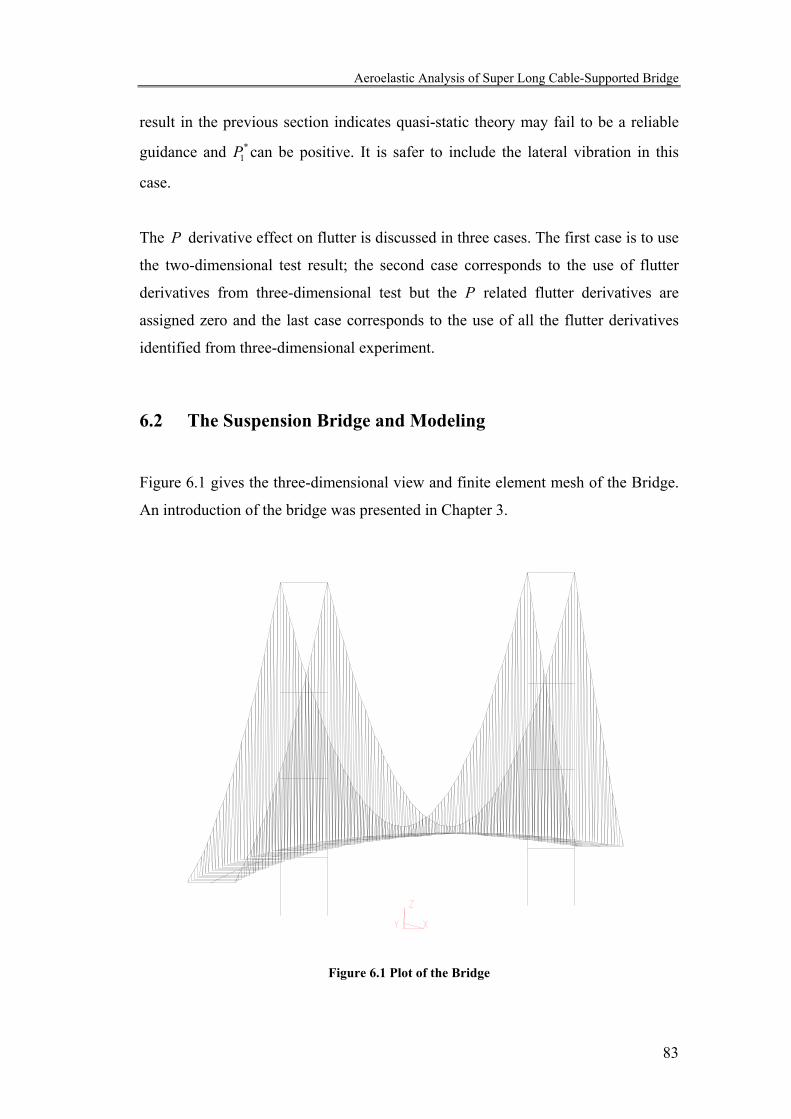
Aeroelastic Analysis of Super Long Cable-Supported Bridge
83
result in the previous section indicates quasi-static theory may fail to be a reliable
guidance and *1P can be positive. It is safer to include the lateral vibration in this
case.
The P derivative effect on flutter is discussed in three cases. The first case is to use
the two-dimensional test result; the second case corresponds to the use of flutter
derivatives from three-dimensional test but the P related flutter derivatives are
assigned zero and the last case corresponds to the use of all the flutter derivatives
identified from three-dimensional experiment.
6.2 The Suspension Bridge and Modeling
Figure 6.1 gives the three-dimensional view and finite element mesh of the Bridge.
An introduction of the bridge was presented in Chapter 3.
Figure 6.1 Plot of the Bridge

Aeroelastic Analysis of Super Long Cable-Supported Bridge
84
Table 6.1 summarizes the material properties and other dimensions required in
calculation. The main span is 1410m, with side span of 530 and 280m. The steel
box-sections are 22m wide and 4.5m deep and the shape is the same as the box
girder sectional model (model B in chapter 3). The towers are box section, 6 by 6 m
at the base and 4.5 by 4.5 at the tower tops.
Table 6.1 Material Properties of the Humber Bridge
Cable
Young’s modulus of cables 193 KN/mm2
Young’s modulus of hangers 140 KN/mm2
Area per hanger 0.0021 m2
Main Span 0.29 m2
Area of each cable Side Span 0.31 m2
Box Girder Deck
Young’s Modulus 200 KN/mm2
Axial area of steal 0.73 m2
Second moment of area for vertical bending 1.940 m4
Second moment of area for lateral bending 37.07 m4
Torsional rigidity 4.5 m4
Towers
Young’s modulus 20 KN/mm2
Average axial material area of each leg 20.37 m2
Average second moment of area of each tower leg for longitudinal
bending 66.8 m4
Average second moment of area of each tower leg for lateral bending 68.24 m4
Average torsional rigidity of each tower leg 113.1 m4
To facilitate the inclusion of an aeroelastic load model, 3-D beam deck formulation
was used to model the deck structure. Spar elements (having no flexural stiffness)
were used to present the main cable and hanger. They have the facility to

Aeroelastic Analysis of Super Long Cable-Supported Bridge
85
accommodate the initial strain value. The tower was analyzed using beam elements
with tension, compression, torsion and bending capabilities.
The modal analysis was conducted by using commercial software, ANSYS. Table
6.2 summarizes the modal analysis results. These resultant frequencies are generally
5-10% higher than the measured value on the prototype (Brownjohn et al. 1987).
Table 6.2 Dynamic Properties of the Bridge
Mode No. Mode Type Frequency
in (Hz)
Modal
damping
iς (%)
1 L, 1st S 0.0688 0
2 V, 1st S 0.1277 0
3 L, 1st AS 0.1591 0
4 V, 1st AS 0.1646 0
5 V, 2nd S 0.1897 0
13 V, 2nd AS 0.2498 0
14 LT, L, 2nd S; T, 1st S 0.2816 0
16 V, 3rd S 0.3246 0
26 V, 3rd AS 0.4022 0.5*
28 T, 1st AS 0.45853 0.5*
Note: S=symmetrical; AS=anti-symmetrical; L: Lateral; V=vertical; LT=lateral-torsion; T=torsion
and *=Assumed value
Structural modes used in flutter boundary computation are normalized with respect to mass matrix.
Figures 6.2.a-6.2.e show the structural mode shapes. These modes are normalized
by mass matrix. In the figures, H, P and A denote, respectively, vertical, lateral and
rotational components of the mode. In mode No. 14 & 28, the rotational component
is multiplied by half of the bridge width, so that its magnitude is comparable to
other components.
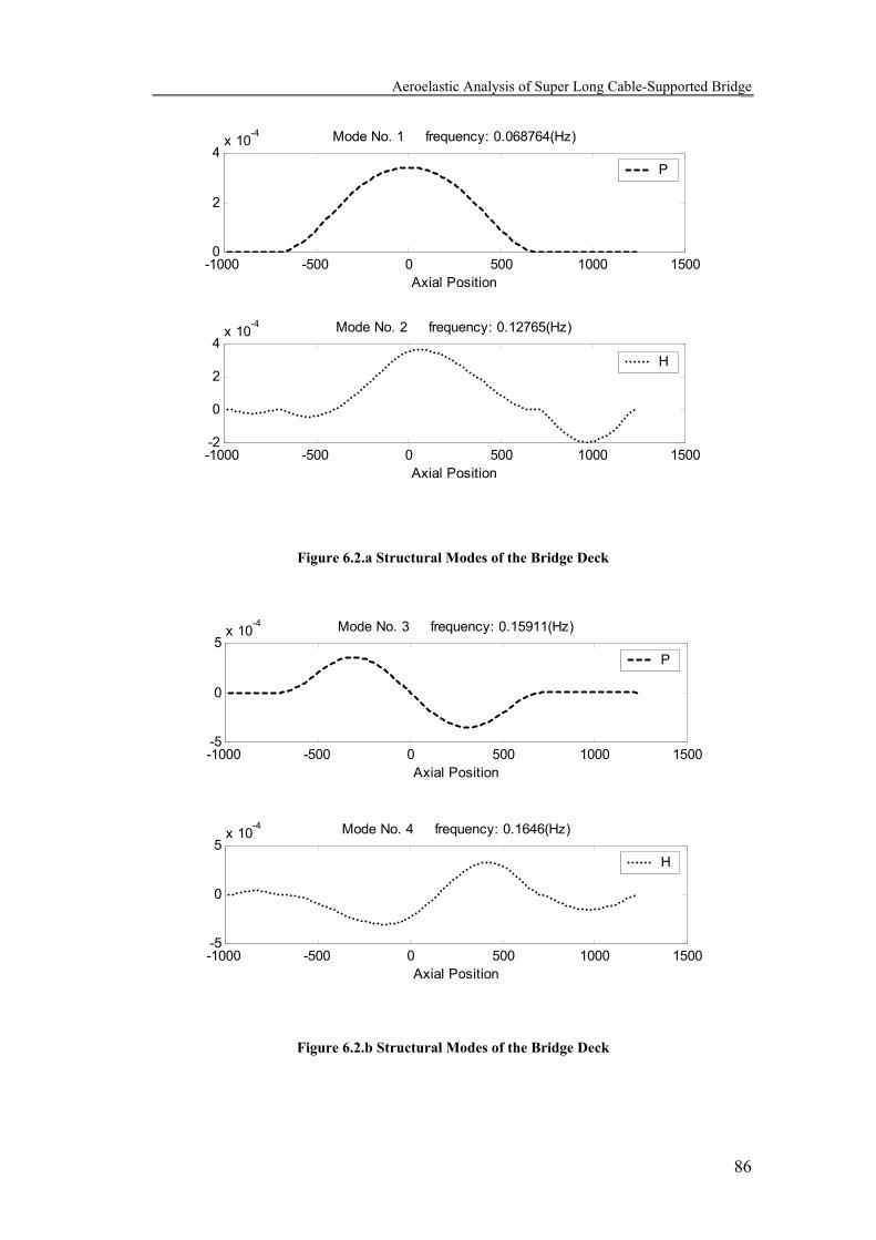
Aeroelastic Analysis of Super Long Cable-Supported Bridge
86
-1000 -500 0 500 1000 15000
2
4x 10⁻⁴ Mode No. 1 frequency: 0.068764(Hz)
Axial Position
P
-1000 -500 0 500 1000 1500-2
0
2
4x 10⁻⁴ Mode No. 2 frequency: 0.12765(Hz)
Axial Position
H
Figure 6.2.a Structural Modes of the Bridge Deck
-1000 -500 0 500 1000 1500-5
0
5x 10⁻⁴ Mode No. 3 frequency: 0.15911(Hz)
Axial Position
P
-1000 -500 0 500 1000 1500-5
0
5x 10⁻⁴ Mode No. 4 frequency: 0.1646(Hz)
Axial Position
H
Figure 6.2.b Structural Modes of the Bridge Deck
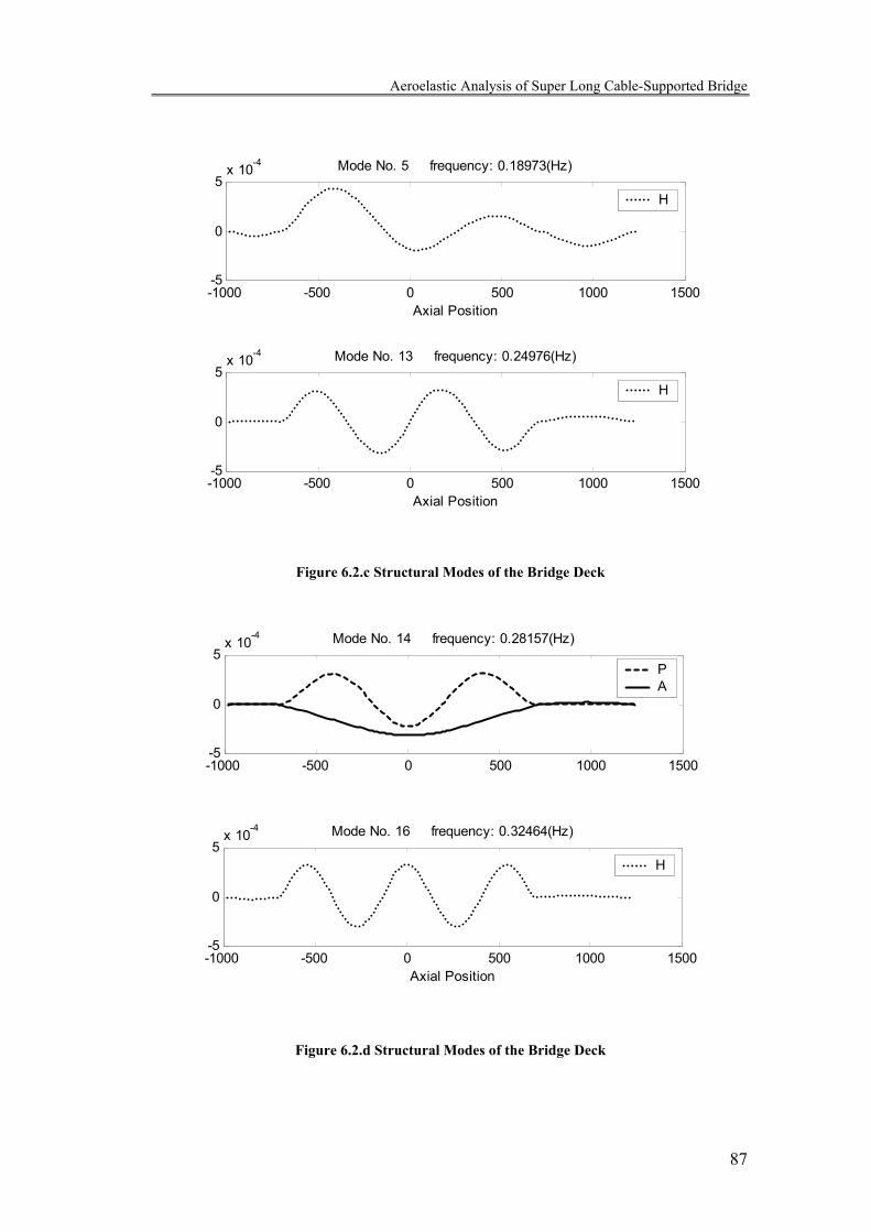
Aeroelastic Analysis of Super Long Cable-Supported Bridge
87
-1000 -500 0 500 1000 1500-5
0
5x 10⁻⁴ Mode No. 5 frequency: 0.18973(Hz)
Axial Position
H
-1000 -500 0 500 1000 1500-5
0
5x 10⁻⁴ Mode No. 13 frequency: 0.24976(Hz)
Axial Position
H
Figure 6.2.c Structural Modes of the Bridge Deck
-1000 -500 0 500 1000 1500-5
0
5x 10⁻⁴ Mode No. 14 frequency: 0.28157(Hz)
PA
-1000 -500 0 500 1000 1500-5
0
5x 10⁻⁴ Mode No. 16 frequency: 0.32464(Hz)
Axial Position
H
Figure 6.2.d Structural Modes of the Bridge Deck

Aeroelastic Analysis of Super Long Cable-Supported Bridge
88
-1000 -500 0 500 1000 1500-5
0
5x 10⁻⁴ Mode No. 26 frequency: 0.40216(Hz)
Axial Position
H
-1000 -500 0 500 1000 1500-1
0
1x 10⁻³
Axial Position
Mode No. 28 frequency: 0.45853(Hz)
A
Figure 6.2.e Structural Modes of the Bridge Deck
These mode shapes are similar to those modes experimentally identified in previous
study (Brownjohn et al. 1987).
After the modal parameters were obtained, they were exported to MATLAB (The
Mathworks 1998) environment to perform the flutter instability prediction.
6.3 Method to Solve the Aeroelastically Influenced Eigenvalue
Problem
Equation (6.1.1) is doubled up since both the real and imaginary parts of the
determinant have to be zero. Corresponding unknowns are reduced frequency K or
wind velocity U and vibration frequency ω . These equations are highly nonlinear
in both unknowns not only through the dependence that appears in the expression of
the elements in impedance matrix, but also through the flutter derivatives that are
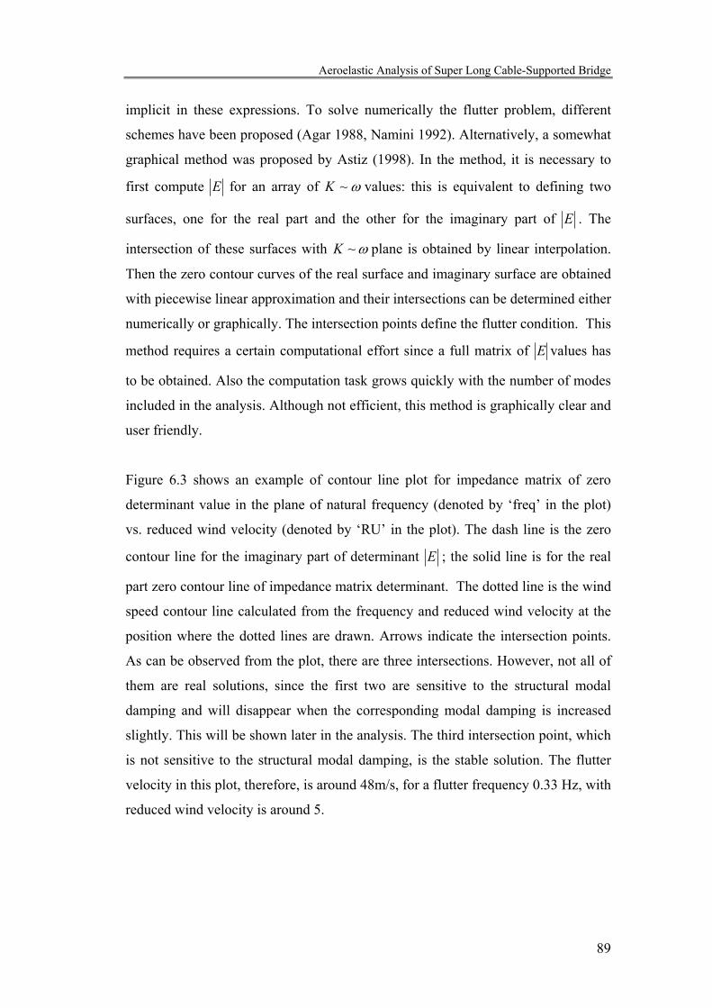
Aeroelastic Analysis of Super Long Cable-Supported Bridge
89
implicit in these expressions. To solve numerically the flutter problem, different
schemes have been proposed (Agar 1988, Namini 1992). Alternatively, a somewhat
graphical method was proposed by Astiz (1998). In the method, it is necessary to
first compute E for an array of ω~K values: this is equivalent to defining two
surfaces, one for the real part and the other for the imaginary part of E . The
intersection of these surfaces with ω~K plane is obtained by linear interpolation.
Then the zero contour curves of the real surface and imaginary surface are obtained
with piecewise linear approximation and their intersections can be determined either
numerically or graphically. The intersection points define the flutter condition. This
method requires a certain computational effort since a full matrix of E values has
to be obtained. Also the computation task grows quickly with the number of modes
included in the analysis. Although not efficient, this method is graphically clear and
user friendly.
Figure 6.3 shows an example of contour line plot for impedance matrix of zero
determinant value in the plane of natural frequency (denoted by ‘freq’ in the plot)
vs. reduced wind velocity (denoted by ‘RU’ in the plot). The dash line is the zero
contour line for the imaginary part of determinant E ; the solid line is for the real
part zero contour line of impedance matrix determinant. The dotted line is the wind
speed contour line calculated from the frequency and reduced wind velocity at the
position where the dotted lines are drawn. Arrows indicate the intersection points.
As can be observed from the plot, there are three intersections. However, not all of
them are real solutions, since the first two are sensitive to the structural modal
damping and will disappear when the corresponding modal damping is increased
slightly. This will be shown later in the analysis. The third intersection point, which
is not sensitive to the structural modal damping, is the stable solution. The flutter
velocity in this plot, therefore, is around 48m/s, for a flutter frequency 0.33 Hz, with
reduced wind velocity is around 5.
Aeroelastic Analysis of Super Long Cable-Supported Bridge
90
2.5 3 3.5 4 4.5 5 5.5 6 6.5 7 7.5 8
0.2
0.25
0.3
0.35
0.4
0.45
0.5
RU
freq
30m/s
50m/s
70m/s
Real Part
Imag Part
Figure 6.3 Sensitivity of E-matrix to Damping Ratio
6.4 Approximating the Impedance Matrix
As mentioned above, the solution of equation (6.1.2) at flutter determines the
participation magnitude of each structural mode. Because the flutter frequency is
solved numerically or graphically, the determinant of impedance matrix obtained at
flutter is not strictly zero, i.e.
0≈fluuter
E (6.4.1)
Directly solving the equation
0=ξflutterE (6.4.2)
Aeroelastic Analysis of Super Long Cable-Supported Bridge
91
will not always give a reasonable result.
Jain (1997) mentioned that before solving the equation, one of the elements in
vector ξ should be preset at a certain value and some care should be exercised in
the assignment of the value, due to the numerical sensitivity of the system at flutter.
Typically for suspension bridges a single torsional mode is the most likely mode to
dominate flutter, while participation of other modes may not significantly alter the
outcome of the analysis. Therefore, Jain (1997) argued that for practical reason, the
preset value should be assigned to the entry corresponding to such flutter
dominating modes; otherwise, misleading result may be obtained.
Although practical, this method is not convincing. Some analytical results of
multimode flutter analysis of long-span bridges indicate that because of the closely
spaced natural frequencies and three-dimensional structural mode shapes, the
aerodynamic coupling mechanism among structural modes becomes complex.
Furthermore, the coupled multimode flutter is not always initiated by the
fundamental symmetric torsional mode (Miyata and Yamada 1988, Agar 1989).
These results seem to be sensitive to the structural and aerodynamic characteristics
of the system.
Therefore, it is needed to find an exact singular matrix E~ , so that the numerically
obtained impedance matrix can be approximated with the main structure of the
impedance matrix being maintained and the solution of equation 0~ =ξE produces
approximately the real eigenvector.
Singular value decomposition (SVD) of a matrix is a good tool to approximate a
matrix around a singular point. If the impedance matrix is decomposed with SVD
TUSVE = , (6.4.3)
where U and V are orthogonal singular vectors matrices, the diagonal singular
value matrix
Aeroelastic Analysis of Super Long Cable-Supported Bridge
92
=
0
1
00S
SS (6.4.4)
is affected by the perturbations in the numerically calculated impedance matrix and
tends to be full rank. The diagonal elements in S are nii ,,2,1, L=σ , and
nσσσ ≥≥≥ ,,21 L . n is the dimension of the E matrix.
By letting some of the last few singular values be zero, i.e.
[ ] 00 =S (6.4.5)
the rank of the matrix E is reduced:
)()( 1SRankSRank = . (6.4.6)
Multiplying Equation (6.4.2) by TU , since matrix U is orthogonal, we have:
00001 =
≈ ξξ TT V
SEU . (6.4.7)
It is easier to solve
[ ] 001 =ξTVS . (6.4.8)
Figure 6.4 shows a representative profile of singular values (S Value in the plot) of
the impedance matrix at flutter. It can be observed that the last point is much closer
to zero than others. It is safe to say this point is generated by the small perturbation
in the impedance matrix, and can be deleted.

Aeroelastic Analysis of Super Long Cable-Supported Bridge
93
0 5 100
2
4
6
8
10
12
S V
aluv
e
0 5 1010-5
10-4
10-3
10-2
10-1
100
101
102
Figure 6.4 Non-dimensional Singular Values at Flutter (2D FD Case, 1st Mode)
One problem that remains is how many singular values should be assigned zero. If
n singular values are assigned zero, that means there are n linearly independent
flutter modes at the given flutter frequency. It seems satisfactory to have one single
flutter mode corresponding to a given flutter frequency in current analysis.
However, there could be more than one flutter mode with the same frequency. This
question is open.
6.5 Description of the Analysis
The analysis adopts flutter derivatives identified from three and two-dimensional
experiments of both transient and ambient type. The relative amplitude effect is
studied by changing the FDs (flutter derivatives) identified by transient vibration to
FDs identified by ambient vibration. The flutter derivatives used are FDs of model
Aeroelastic Analysis of Super Long Cable-Supported Bridge
94
B presented in Chapter 5. Some of FDs are smoothed according to their trend to
avoid unexpected fluctuations in the calculation.
6.5.1 Analytical Cases
In the first step, the analysis is performed with 2D FDs, and the critical wind speeds
for flutter are obtained. In the second step, 2D FDs are obtained from 3D FDs by
setting the P related derivatives to zero for all the reduced velocities, i.e.
0~ *6
*1 =PP ; 0*
6*5 == AA ; 0*
6*5 == HH . In the third step, analysis is carried out
with 3D FDs. These three steps repeat for transient and ambient cases. The first step
indicates that there is no self-excited load relating to lateral structural vibration; the
second step assumes that there is self-excited load relating to lateral vibration but it
is neglected; the third step fully considers self-excited forced in 3DOF.
Note that the flutter derivatives ( *4
*1 ~ HH , *
4*1 ~ AA ) identified from 2D
experiment might not always be consistent with the results of 3D experiment. There
could be some effects of the restriction in the third dimension because in the
experimental setup of the first step, the structure is actually being restricted in the
lateral direction. If the aeroelastic coupling between the vertical and lateral
vibration, or between rotational and lateral vibration is not negligible, and must be
taken into consideration, the results could be different in step one and step two.
In total, 10 structural modes are included to be linearly combined to represent the
flutter mode in this analysis. Table 6.2 shows the structural modes included in the
flutter analysis. Modal damping of the first eight modes was assigned to be zero, so
that the analysis would be conservative. It was found that the flutter occurs at very
low wind speed if the last two modes have zero damping (as shown in Figure 6.3).
Therefore, accepting 0.5% damping is assigned to both modes. Considering that the
method of predicting flutter is a pure numerical procedure and the aeroelastic
parameters are experimentally measured, the sensitivity of the numerical procedure
does not necessarily mean that the structure’s flutter is sensitive to the structural
Aeroelastic Analysis of Super Long Cable-Supported Bridge
95
damping in the mechanical sense. The sensitivity, therefore, may reflect the “virtual
reality in the numerical world”. A physically meaningful solution will be robust to
the disturbances in the parameters, e.g. errors in the identified flutter derivatives. If
it is noticed that the geometrical features of the three intersection points in Figure
6.3 are different, it may be reasonable to argue that the tangential intersection points
(the first two intersection point in Figure 6.3) of the continuous lines and dashed
lines may be not reliable. The geometric feature is ill conditioned. The
perpendicular intersection point (the third intersection point in Figure 6.3) is more
reliable than the first two. If the first two intersection points are sensitive to
perturbations in the identified parameters (additional structural damping is
equivalent to a perturbation in the flutter derivatives), the solutions corresponding to
them may not be reliable.
Table 6.3 summarizes the analysis and the corresponding flutter wind speeds and
frequencies. Figures (6.5-6.7) show the plot of contour lines for impedance matrix
of zero determinant value. The intersection points of the solid line (zero value
contour line of real part of the determination of the impedance matrix) and the
dashed line (zero value contour line of imaginary part) define the flutter condition.
Table 6.3 Flutter Speeds & Frequencies in Different Combinations
Case Structural Modes Included Flutter Speed
flutterU (m/s)
Flutter
Frequency
flutterf (Hz)
1. Transient 1, 2, 3, 4, 5, 13, 14, 16, 26, 28 52.7 75.9 0.267 0.3922D FD
2. Ambient 1, 2, 3, 4, 5, 13, 14, 16, 26, 28 NA NA
3. Transient 1, 2, 3, 4, 5, 13, 14, 16, 26, 28 38.5 51.1 0.252 0.3412D from 3D
4. Ambient 1, 2, 3, 4, 5, 13, 14, 16, 26, 28 NA NA
5. Transient 1, 2, 3, 4, 5, 13, 14, 16, 26, 28 48.2 NA 0.332 NA 3D
6. Ambient 1, 2, 3, 4, 5, 13, 14, 16, 26, 28 NA NA
NA: Solution not found within the reduce velocity range covered by experiment

Aeroelastic Analysis of Super Long Cable-Supported Bridge
96
2.5 3 3.5 4 4.5 5 5.5 6 6.5 7 7.5 8
0.2
0.25
0.3
0.35
0.4
0.45
0.5
RU
freq
0
30m/s
50m/s
70m/s
Real Part
Imag Part
Figure 6.5 E Matrix of 2D FD
2.5 3 3.5 4 4.5 5 5.5 6 6.5 7 7.5 8
0.2
0.25
0.3
0.35
0.4
0.45
0.5
RU
freq
30m/s
50m/s
70m/s
Real Part
Imag Part
Figure 6.6 E Matrix From 2D FD By Deleting P Related FD
Aeroelastic Analysis of Super Long Cable-Supported Bridge
97
2.5 3 3.5 4 4.5 5 5.5 6 6.5 7 7.5 8
0.2
0.25
0.3
0.35
0.4
0.45
0.5
RU
freq
30m/s
50m/s
70m/s
Real Part
Imag Part
Figure 6.7 E Matrix From 3D FD
6.5.2 Effect of Relative Amplitude
The effects of relative amplitude are manifested by replacing the flutter derivatives
identified from transient vibration with those identified from ambient vibration. As
can be observed in Table 6.3, while the flutter derivatives identified from transient
vibration may produce flutter condition, the flutter derivatives from ambient
response are aeroelastically stable. No flutter occurs in all the study cases within the
range of reduced velocity covered by experiments. This indicates that when the
modal amplitude of a particular mode is smaller than the ambient vibration
amplitude it needs additional excitations, strong gust, for example, to put it outside
the “ambient vibration envelope” to be a flutter mode.
The weakness of the argument is that the ambient vibrations may have different
wind spectra in sectional model and full-scale studies. In view of this, in the
discussion of the relative modal amplitude effect on flutter, it is an open question

Aeroelastic Analysis of Super Long Cable-Supported Bridge
98
whether or not the experiment to identify the flutter derivatives based on sectional
model testing is applicable to the full bridge. However, the logic is that if there is no
such effect as relative amplitude effect on flutter, there should be no big difference
between the analytical prediction results by using either transient or ambient
vibration testing. Now that there is a difference between these two analyses, there
must be relative amplitude effect. Although the quantitative significance is
questionable, the qualitative significance stands.
A major conjecture relating to relative amplitude effect is that if turbulence exists in
the oncoming flow or is generated by the structure itself, the “ambient vibration
envelope” will grow, making it harder to put the modal amplitude outside the
envelope. Therefore the structure will become more stable. As has been indicated in
the previous study, the discussions on turbulence effect on flutter follow two ways,
one is to resort to stochastic differential equation, the other is to measure flutter
derivatives in turbulence with transient free or forced sinusoidal vibration. Neither
of these two ways, however, considers the relative amplitude effect on flutter
derivatives, i.e. the interaction between the buffeting force and interactive force, and
its further effect on flutter boundary.
6.5.3 Effect of Lateral Flutter Derivatives
As indicated above, there are three case studies to investigate the lateral flutter
derivative effect on flutter. The quasi-static theory is not included, since the
experimental result from transient vibration appears not to be consistent with it.
Although the ambient vibration testing gives rise to negative *1P , its resultant flutter
derivatives are aeroelastically stable, suggesting there is no need to include quasi-
static theory in this case.
The lowest wind speed for flutter occurs in the second step of the analysis, i.e. the
case which uses the 3D flutter derivatives with all P related flutter derivatives
being assigned zero. The flutter wind velocity in this case is 38.5m/s, and the flutter
Aeroelastic Analysis of Super Long Cable-Supported Bridge
99
frequency is 0.252Hz. 2D flutter derivatives give rise to the highest flutter wind
speed: 53m/s, and flutter frequency 0.267Hz. 3D flutter derivatives produce the
flutter wind velocity 48m/s and flutter frequency 0.332Hz.
It can be observed that there are two flutter modes found in analysis with 2D flutter
derivatives and 3D flutter derivatives with all P related flutter derivatives being
assigned zero, but only one flutter mode is found for the 3D flutter analysis. The P
derivatives push the lower one of the two unstable modes to higher reduced wind
velocity, which is outside the experimental range. The flutter mode shapes are
shown in Figure (6.8-6.12). Every mode vector x is normalized so that 12=x .
The flutter mode shape in the 3D flutter derivative case is close to the second flutter
mode in the other two cases. Table 6.4 summarizes the participation factors of the
structural modes at flutter. All the figures indicate that the vertical motion
predominates in the flutter mode.
Summary
Flutter derivatives of a partially streamlined box girder section identified from
transient and ambient vibration testing were used to manifest the relative amplitude
effect on flutter. The flutter derivatives from ambient vibration were found
aeroelastically stable. Therefore, the relative amplitude effect has a stabilizing
consequence. The relative amplitude effect may be used to study the turbulence
effect on flutter, but further studies are needed.
The analysis was carried out with 3DOF and 2DOF flutter derivatives, so that the
effect of lateral flutter derivatives can be investigated. In comparison with the two
study cases where flutter derivatives used are 2D or 3D, the analysis using 3D
flutter with P related flutter derivatives being assigned zero gives rise to the lowest
flutter wind speed. All these discussions are limited to the specific section type
under study.
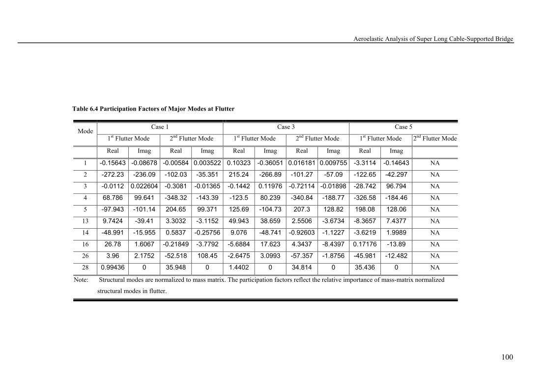
Aeroelastic Analysis of Super Long Cable-Supported Bridge
100
Table 6.4 Participation Factors of Major Modes at Flutter
Case 1 Case 3 Case 5 Mode
1st Flutter Mode 2nd Flutter Mode 1st Flutter Mode 2nd Flutter Mode 1st Flutter Mode 2nd Flutter Mode
Real Imag Real Imag Real Imag Real Imag Real Imag
1 -0.15643 -0.08678 -0.00584 0.003522 0.10323 -0.36051 0.016181 0.009755 -3.3114 -0.14643 NA
2 -272.23 -236.09 -102.03 -35.351 215.24 -266.89 -101.27 -57.09 -122.65 -42.297 NA
3 -0.0112 0.022604 -0.3081 -0.01365 -0.1442 0.11976 -0.72114 -0.01898 -28.742 96.794 NA
4 68.786 99.641 -348.32 -143.39 -123.5 80.239 -340.84 -188.77 -326.58 -184.46 NA
5 -97.943 -101.14 204.65 99.371 125.69 -104.73 207.3 128.82 198.08 128.06 NA
13 9.7424 -39.41 3.3032 -3.1152 49.943 38.659 2.5506 -3.6734 -8.3657 7.4377 NA
14 -48.991 -15.955 0.5837 -0.25756 9.076 -48.741 -0.92603 -1.1227 -3.6219 1.9989 NA
16 26.78 1.6067 -0.21849 -3.7792 -5.6884 17.623 4.3437 -8.4397 0.17176 -13.89 NA
26 3.96 2.1752 -52.518 108.45 -2.6475 3.0993 -57.357 -1.8756 -45.981 -12.482 NA
28 0.99436 0 35.948 0 1.4402 0 34.814 0 35.436 0 NA
Note: Structural modes are normalized to mass matrix. The participation factors reflect the relative importance of mass-matrix normalized
structural modes in flutter.
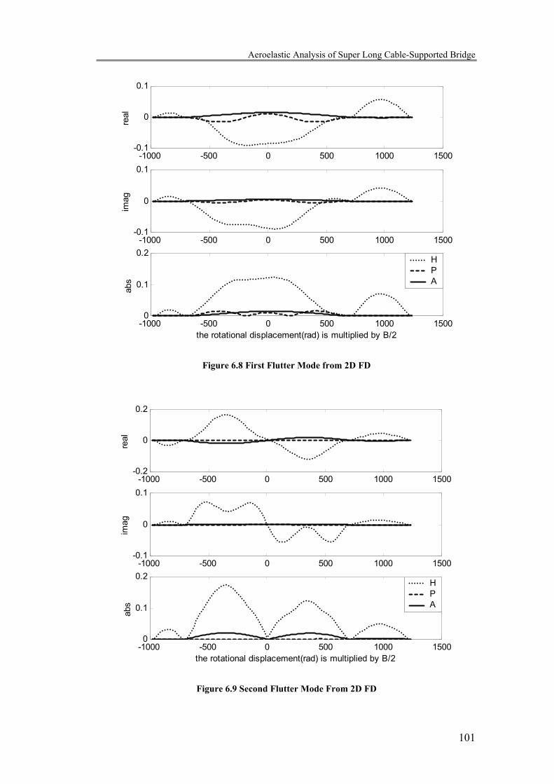
Aeroelastic Analysis of Super Long Cable-Supported Bridge
101
-1000 -500 0 500 1000 1500-0.1
0
0.1
real
-1000 -500 0 500 1000 1500-0.1
0
0.1
imag
-1000 -500 0 500 1000 15000
0.1
0.2
abs
the rotational displacement(rad) is multiplied by B/2
HPA
Figure 6.8 First Flutter Mode from 2D FD
-1000 -500 0 500 1000 1500-0.2
0
0.2
real
-1000 -500 0 500 1000 1500-0.1
0
0.1
imag
-1000 -500 0 500 1000 15000
0.1
0.2
abs
the rotational displacement(rad) is multiplied by B/2
HPA
Figure 6.9 Second Flutter Mode From 2D FD
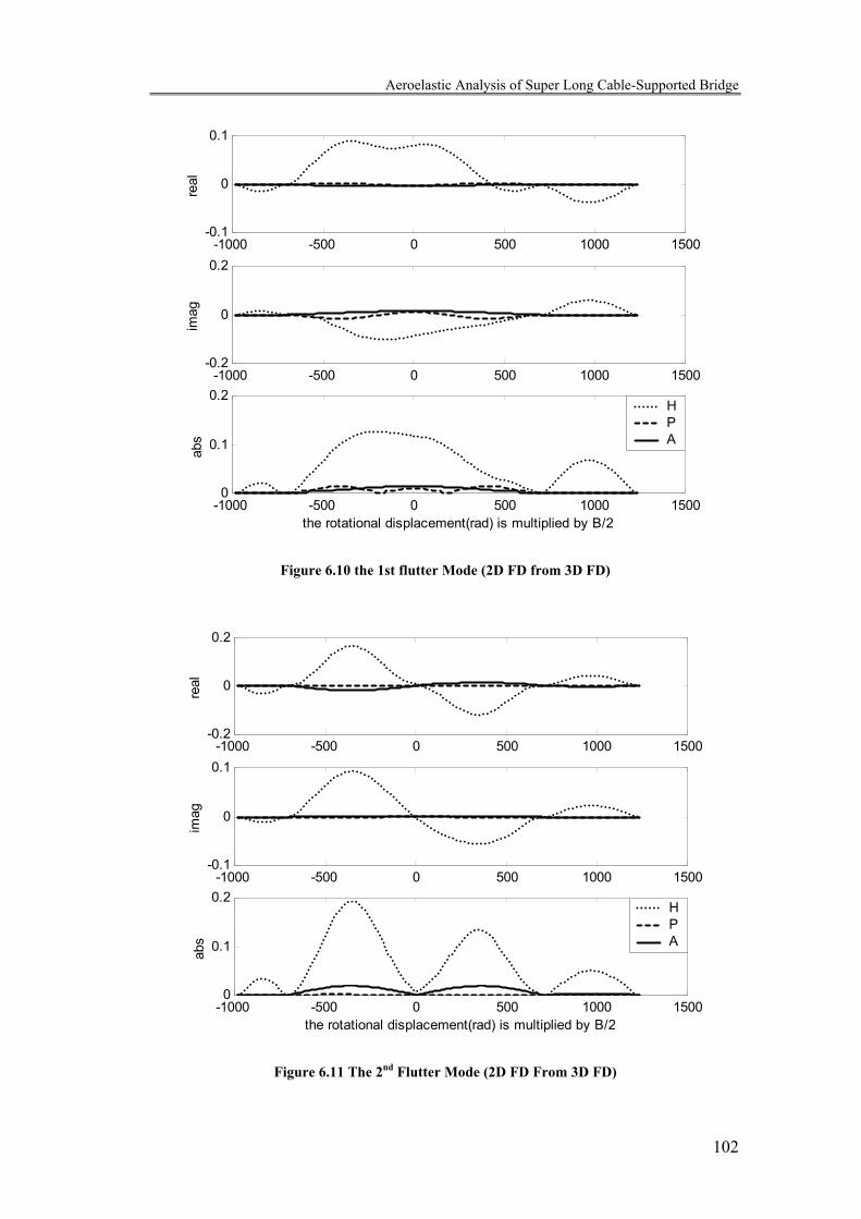
Aeroelastic Analysis of Super Long Cable-Supported Bridge
102
-1000 -500 0 500 1000 1500-0.1
0
0.1
real
-1000 -500 0 500 1000 1500-0.2
0
0.2
imag
-1000 -500 0 500 1000 15000
0.1
0.2
abs
the rotational displacement(rad) is multiplied by B/2
HPA
Figure 6.10 the 1st flutter Mode (2D FD from 3D FD)
-1000 -500 0 500 1000 1500-0.2
0
0.2
real
-1000 -500 0 500 1000 1500-0.1
0
0.1
imag
-1000 -500 0 500 1000 15000
0.1
0.2
abs
the rotational displacement(rad) is multiplied by B/2
HPA
Figure 6.11 The 2nd Flutter Mode (2D FD From 3D FD)
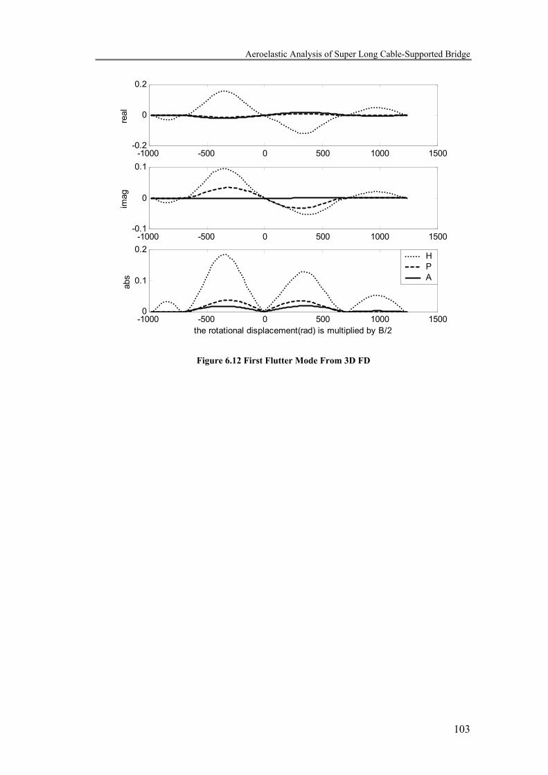
Aeroelastic Analysis of Super Long Cable-Supported Bridge
103
-1000 -500 0 500 1000 1500-0.2
0
0.2
real
-1000 -500 0 500 1000 1500-0.1
0
0.1
imag
-1000 -500 0 500 1000 15000
0.1
0.2
abs
the rotational displacement(rad) is multiplied by B/2
HPA
Figure 6.12 First Flutter Mode From 3D FD
Aeroelastic Analysis of Super Long Cable-Supported Bridge
104
CHAPTER SEVEN
Time Domain Formulation of Self-Excited Forces on
Bridge Decks for Wind Tunnel Experiments
Abstract
Time domain formulation of the self-excited wind forces on bridge decks often
employs indicial functions. The usual practice in bridge aeroelasticity is to
transform the flutter derivative model to time domain. Studies in previous chapters
suggested, however, that the relative amplitude effect, i.e. the structural oscillation
amplitude relative to the ambient vibration amplitude on flutter derivatives, needs
to be considered. This effect indicates that although self-excited wind forces are
linear when the pulse response of an elastically supported body is smooth, they are
nonlinear when the motion is significantly affected by the buffeting forces. The
nonlinearity may cause unnoticed error in the transformation. An alternative is to
treat the self-excited forces (SEF) generation mechanism as a separate dynamic
system, so that the relative amplitude effect can be evaluated in more details. In this
part, SEF generation system coupled with the rigid bridge deck system is proposed
to overcome the difficulties in the measurement and derivation of the time domain
representation of self-excited forces on bridge decks. This expression can be linked

Aeroelastic Analysis of Super Long Cable-Supported Bridge
105
to the frequency-time-domain-hybrid flutter derivative model, and a transform
relationship between the two models is suggested. The SEF model enables the
treatment of the self-excited forces as an independent dynamic system and identify it
directly. This may change significantly the way of doing wind tunnel experiments to
formulate the self-excited wind force and make the experiment more in line with
system theory.
7.1 Introduction
The most fundamental task of bridge aeroelasticity lies in the formulation of the
self-excited forces, the wind load caused by the movement of the structure. Some of
the historical works were reviewed in Chapter 2. They are summarized in the next
several paragraphs.
Theodorsen (1935) derived the theoretical description of the unsteady aerodynamic
forces on the efficient airfoil under sinusoidal motion by employing the reduced
frequency dependent Theodorsen’s circulation function. Theodorsen and Garrick
(1943) further extended the work to characterize the non-stationary flow about a
wing-aileron-tab combination. Following Sears (1940) and Luke and Dengler
(1951), Edwards (1977) showed that these results could be generalized for arbitrary
motion. The unsteady aerodynamic force thus can be formulated by a reduced-
frequency dependent aerodynamic influence matrix. In time domain, Wagner
(1925) showed the lift evolution with dimensionless time acting on a theoretical flat
airfoil given a step change in angle of attack. Kussner (1936) considered the
problem of an airfoil with forward flight velocity penetrating a uniform vertical gust
of infinite downstream extent and vertical velocity. Sears (1940) derived the
corresponding oscillatory lift for a gust velocity distribution that is sinusoidal. Jones
(1941) introduced rational approximations of the unsteady loads.
However, the signature turbulence, in the case of efficient airfoils in smooth flow, is
intentionally reduced by careful streamlining with notable attention to introduction

Aeroelastic Analysis of Super Long Cable-Supported Bridge
106
of a sharp trailing edge. For bluff bodies, the situation is different. The use of
Theodorsen aerodynamics for bluff bodies is not guarantied to be correct. In view
of this, the formulation of self-excited forces on a civil engineering structures, such
as a bridge decks, is more experimental than theoretical. Scanlan and Tomko (1971)
suggested reduced frequency dependent flutter derivatives be used in the modelling
of self-excited wind load on bridge deck.
In the time domain formulation of self-excited forces on a bridge deck, indicial
functions are the most important tools when the structure is subjected to arbitrary
motion. Scanlan et al. (1974) studied the aeroelastic moment on a bluff bridge deck
due to indicial angular movement. The characteristic of corresponding indicial
function of a bridge, i.e. the rotational aerodynamic damping due to the rotational
motion, according to their experiment, is strongly different from those of the
corresponding functions of airfoils. It was showed that the relationship between the
flutter derivatives and the indicial function is obtained by recognizing that for a
sinusoidal motion, the Duhammel integral is of the nature of a Fourier transform
(Sabzevari, 1971) and the inverse transform of frequency domain expression should
then produce the indicial function. Other studies (Yoshimura and Nakamura 1979)
to measure indicial functions are available. Figure 7.1 shows the indicial functions
with different structural forms. The Jones approximation is for efficient airfoils. The
other two curves are experimental measurements from bluff bridge decks. Scanlan
et al (1974) used an exponential approximation form with two exponential terms to
curve fit the experimental data from a truss structure. The measurement of
Yoshimura and Nakamura (1979) is a direct measurement of indicial aerodynamic
moment response of moving bluff prismatic sections of H or T type in still air. This
curve is scaled to match the magnitude of other curves; it is shown here only
qualitatively. Striking differences can be observed from the exponential
approximation curves: an initial steep rise from a low negative value to a peak,
which “overshoots” the steady state value, then settles down asymptotically. The
oscillating component in the curve by Yoshimura and Nakamura is clear and cannot
be neglected.

Aeroelastic Analysis of Super Long Cable-Supported Bridge
107
However, the direct measurement of indicial functions is neither easy, nor
conventional. Bucher and Lin (1988), and Chen et al. (2000a, 2000b) treated the
surrounding airflow as a set of filter like devices in generating self-excited forces on
bridge by transforming the frequency domain flutter derivatives to time domain for
the flutter and buffeting analysis of cable supported bridges.
0 1 2 3 4 5 6 7 8-1
-0.5
0
0.5
1
1.5
2
2.5
3
3.5
Dimensionless Time s
Val
ue o
f Ind
icia
l Fun
ctio
n
Scanlan et al
Yoshimura & Nakamura
Jones
Figure 7.1 Indicial Functions of Different Kinds
7.2 Relative Amplitude Effect on the Transformation of Flutter Derivative
Model to Time Domain
The relative amplitude effect is defined as the effect of triggered vibration
amplitude of the model relative to “structural noise” in the vibration due to the
ambient wind excitation. As have been observed in previous part of the study on the
identification of flutter derivatives from transient and ambient vibration, the relative
Aeroelastic Analysis of Super Long Cable-Supported Bridge
108
amplitude effect on flutter derivatives cannot be neglected. The effect of relative
amplitude on flutter derivatives and on the flutter boundary reveals, from the
structural point of view, a complex relationship between the self-excited forces and
the “structural vibration noise” due to signature turbulence related buffeting forces.
Although the aeroelastic forces are linear when the body motion due to an external
trigger is not affected significantly by the signature turbulence, they are nonlinear
when the noise component in the vibration due to the signature turbulence related
buffeting forces couldn’t be neglected.
In view of this, it may not be valid in some cases to transform the flutter derivative
model measured under sinusoidal or exponentially modified oscillation to time
domain for general-purpose analysis. Alternative models for the identification of
interactive forces from experiments may be favourable.
7.3 State Space Model for SEF Generation System
In this section, the SEF generation system is dealt with as a sperate dynamic
system. The effort is not to provide a nonlinear model, but to linearize the nonlinear
behaviour at different values of relative amplitude so that further experiment can be
done to study the interactive forces on a bridge deck at different relative amplitude
either in time domain format or conventional time-frequency-domain hybrid format.
It is speculated that the nonlinearity in the self-excited wind force on a bridge deck
is due to the change of the relative amplitude of the body vibration and can be
linearized if the relative amplitude is kept constant.
7.3.1 The Model
If the bridge deck motion is known, the nonlinear SEF generation mechanism can
be modeled approximately by a linear time invariant system, it is possible to
identify a linear state space model with a minimum number of states from the
Aeroelastic Analysis of Super Long Cable-Supported Bridge
109
experimental data to approximate the input-output relationship. The SEF system is
coupled with the bridge deck sectional model motion: the rigid body system gives
excitations to the SEF generation system and receives feedback from it.
The equation of the sectional model motion is formulated as:
[ ] [ ] [ ] buffsef ffxKxCxM +=++ &&& (7.3.1)
in which Tphx α= is the displacement vector comprising of vertical, lateral
and rotational motion, [ ]M is structural mass matrix, [ ]C is the structural damping;
[ ]K structural stiffness. bufff is the buffeting force vector due to the fluctuating
component in the oncoming flow and signature turbulence generated by the bluff
body itself. This term is considered independent of the structural motion. seff is the
self-excited force, i.e. the feedback from the SEF generation system to the structural
system.
Changing equation (7.3.1) to dimensionless time s domain via
tBUs = (7.3.2)
where s is the dimensionless time; U is the wind velocity, B is the width of the
bridge deck, one has
[ ] [ ] [ ] [ ]
[ ] ))((
)()()(
12
12
1
sffMUB
sxKMUBsxCM
UBsx
buffsef +
=
+′
+′′
−
−−
(7.3.3)
where ′ and ″ are the first and second derivatives of corresponding variable with
respect to dimensionless time s , respectively.
Aeroelastic Analysis of Super Long Cable-Supported Bridge
110
The state space form of equation (7.3.3) is:
)()(
))()(()()(
sXCsY
sfsfBsXAsX
s
buffsefss
=
++=′ (7.3.4)
with state vector
TsspshsspshsX )()()()()()()( αα ′′′= (7.3.5)
and the state matrix
[ ] [ ] [ ] [ ]
−
−= −− CM
UBKM
UB
IAs 11
20
. (7.3.6)
The input matrix for self-excited forces and buffeting forces vector is
[ ]
= −1
20
MUBBs ; (7.3.7)
and the output matrix is
=
000100000010000001
sC . (7.3.8)
Similarly, the state space formulation for the flutter derivative model is obtained by
using reduced frequency dependent matrices [ ]aeroC and [ ]aeroK :
[ ] [ ] )()()( txKtxCtf aeroaerosef += & . (7.3.9)
Aeroelastic Analysis of Super Long Cable-Supported Bridge
111
Therefore equation (7.3.4) can be rewritten as
)()(
)()()(
sXCsY
sfBsXAsX
s
buffsf
s
=
+=′ (7.3.10)
where
[ ] [ ] [ ] [ ]
−
−= −−
effeff
fs CM
UBKM
UB
IA 11
20
(7.3.11)
[ ] [ ] [ ]aeroeff KKK −= and (7.3.12)
[ ] [ ] [ ]aeroeff CCC −= (7.3.13)
SEF generation system is also formulated by state space equations in dimensionless
time domain. One question is how to determine the input of the SEF generation
system. It can be argued that the dimensionless time derivative of the rigid body
state vector can be considered as the input “force” of the SEF system.
A proof is due to Bisplinghoff and Ashley (1962). They have pointed out that
indicial response functions corresponding to lift and moment due, respectively, to
step changes in effective angle of attack and effective rate of change of angle of
attack, should be used to formulate the unsteady aeroelastic force on airfoil. Lin and
Yang (1983) held the same idea and suggested impulse response functions of the
self-excited forces due to velocity and acceleration of the rigid body, respectively. It
is justified to argue that the time derivative of rigid body state vector, i.e. )(sXdsd ,
can be the input of SEF system.
The SEF system may be modeled by a linear state space model, with order up to
experimental determination, in dimensionless time domain:

Aeroelastic Analysis of Super Long Cable-Supported Bridge
112
)()(
)()()(
sfCsf
sXdsdBsFfsf
fsef
f
=
+=′ (7.3.14)
in which )(sf is the 1×n state vector of SEF system,
)(sf ′ is the dimensionless time derivative of )(sf with respect to dimensionless
time,
F is the nn× square state matrix,
fB is the 6×n input matrix,
fC is the n×3 output matrix.
The value of n , i.e. the system order, is to be determined from experimental data.
Equation (7.3.14) reveals a deterministic relationship between the dimensionless
time derivative of rigid body state vector, )(sXdsd and the self-excited forces
)(sfsef . By no means will this imply that there is a similar relation between
)(sX and )(sfsef . The determinability of the relationship between )(sX and )(sfsef
depends on specific motion patterns of the rigid body. Using the input-output
relation )()( sfsXdsd
sef→ is physically different from using )()( sfsX sef→ when
the rigid body motion pattern is more general.
The coupled system governed by equation (7.3.4) and (7.3.14) can be expressed in
the form of the simulation diagram shown in Figure 7.2. In the diagram, the self-
excited forces system and the bridge deck system are referred to as SEF and BDS,
respectively. The SEF system takes the dimensionless time derivative of the BDS
state vector as its input and returns the self-excited forces as output to the BDS as a
part of its input.
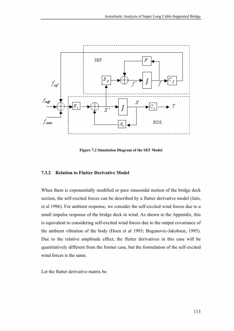
Aeroelastic Analysis of Super Long Cable-Supported Bridge
113
Figure 7.2 Simulation Diagram of the SEF Model
7.3.2 Relation to Flutter Derivative Model
When there is exponentially modified or pure sinusoidal motion of the bridge deck
section, the self-excited forces can be described by a flutter derivative model (Jain,
et al 1996). For ambient response, we consider the self-excited wind forces due to a
small impulse response of the bridge deck in wind. As shown in the Appendix, this
is equivalent to considering self-excited wind forces due to the output covariance of
the ambient vibration of the body (Hoen et al 1993; Bogunovic-Jakobsen, 1995).
Due to the relative amplitude effect, the flutter derivatives in this case will be
quantitatively different from the former case, but the formulation of the self-excited
wind forces is the same.
Let the flutter derivative matrix be

Aeroelastic Analysis of Super Long Cable-Supported Bridge
114
[ ]
=Η
*2
*5
*1
*3
2*6
2*4
2
*2
*5
*1
*3
2*6
2*
4
2
*2
*5
*1
*3
2*6
2*4
2
)(
KAABKA
BKAKA
BKA
BK
KPPBKP
BKPKP
BKP
BK
KHHBKH
BKHKH
BKH
BK
K (7.3.15)
The self-excited forces model is rewritten in a matrix form:
[ ] )()(21)( 2 sXKBUsf sef Η= ρ (7.3.16)
in which Taeaeaesef MDLf = is the self-excited lift drag and moment forces, ρ
is the air density, UBK ω
= is the reduced frequency and 6,1,,, *** K=iAPH iii are
flutter derivatives.
It is possible to convert SEF system model to retrieve flutter derivatives. It seems
easier to be solved in a different format by using Duhammel integral to represent
the “fluid memory”. The “force” term is the time derivative of rigid body state
vector:
[ ]∫ ∞−−Φ=
s
sef dXddsBUf σσσ
σρ )()(21 2 (7.3.17)
in which
[ ] fFs
f BeCsBU =Φ )(21 2ρ (7.3.18)
is the pulse response function of SEF.
The relationship between the time-frequency domain hybrid model and the SEF
system model can be developed as follows. Substitute the rigid body state space
equation (7.3.10) into (7.3.17) and equate to (7.3.16):

Aeroelastic Analysis of Super Long Cable-Supported Bridge
115
[ ] [ ] σσσσ dfBXAssXKH sbuffs
fs∫ +−Φ= ∞− )()()()()( . (7.3.19)
Change the integration variable σ to στ −= s
[ ] [ ] [ ]∫∞∞ −Φ+∫ −Φ=
00 )()()()()()( ττττττ dsfBdsXAsXKH buffsf
s . (7.3.20)
Taking Laplace transform and using convolution property, we have
[ ] [ ] )()()()( KfBKXAKXKH buffsf
s +Φ= (7.3.21)
in which, an over bar denotes Laplace transform.
For the rigid body state space equation (7.3.10), because the buffeting force is
considered as process noise, which is white around the reduced natural frequency,
its magnitude should be much smaller that that of the state vector. Therefore
)()( KfBKXA buffsf
s >> . (7.3.22)
The covariance function equation (A.6) corresponds to the noise free case,
i.e. 0)( =Kfbuff .
Therefore, in both cases equation (7.3.21) yields
[ ] [ ] )()()( KXAKXKH fs⋅Φ≈ . (7.3.23)
There is no particular requirement for )(KX , therefore, the general relationship
between the flutter-derivative matrix and the transfer function of the SEF system
matrix is:
[ ] [ ]( ) 1)()( −Η≈Φ f
sAKK . (7.3.24)
Aeroelastic Analysis of Super Long Cable-Supported Bridge
116
7.3.3 The Transformation in Modal Coordinates
One observation is that the transformation depends on matrix ( ) 1−fsA , which
consists of aeroelastic coupling due to the self-excited forces in addition to the
structural properties. If the motion is decoupled, e.g. in sinusoidal rotational motion,
the system matrix must have the following format:
−
=0
02K
IA f
s , (7.3.25)
so that the aeroelastic matrix is
[ ] [ ]*2
*3
2 KAAK=Η , (7.3.26)
and the transfer function is
[ ] [ ][ ] [ ]*3
*2
-1s
fsA AKAHMM −==ΦΦ ′′′ αα . (7.3.27)
Because the state vector is
TiKsiKs eiKxexsX 00)( = , (7.3.28)
we define an impulse function for moment due to the rotational movement as
αα ′′′ Φ+Φ=Φ MaMM iK (7.3.29)
so that
][ *3
*2 iAAKM −=Φ α . (7.3.30)
This relation is valid for single DOF transfer function and flutter derivatives. For
multi-DOF in the α,, ph coordinates, the transformation of [ ])(KH into [ ])(kΦ
involves the state matrix of the aeroelastically-influenced system, which couples the
Aeroelastic Analysis of Super Long Cable-Supported Bridge
117
elements in matrix [ ])(KH to produce those in matrix [ ])(kΦ . For free vibrations,
the aeroelastic coupling is not always weak, the modal coordinate may be different
from the α,, ph coordinate. If modal coordinates [ ]ϕ are adopted,
[ ] )()( ssX ξϕ= (7.3.31)
it gives:
[ ][ ] [ ]ϕϕ Φ=Λ −1H (7.3.32)
in which
[ ] [ ][ ]ϕϕ HH = , (7.3.33)
[ ] [ ][ ]ϕϕ Φ=Φ , (7.3.34)
and
[ ] [ ] [ ][ ]
==Λ −
22
21
1
n
fs
K
KA Oϕϕ . (7.3.35)
nKK 21 ,..., is reduced natural frequency.
7.4 Suggestions for Future Experiments
Due to the relative amplitude effect, the self-excited wind forces are nonlinear. By
using the SEF model, it is possible to study the effect in more details. The practice
may need non-contact active drivers to force the model so that the model is not
constrained by the forcing device as it is in the case of conventional forced
vibration testing. Since the relative amplitude effect will vanish if the buffeting
response accounts for only a small percentage of the total signal energy, the non-
contact driving device is vital to the study.
If the driving force is sinusoidal, the experiment will be like the conventional forced
vibration testing. By choosing the magnitude of the driving force, the experiment
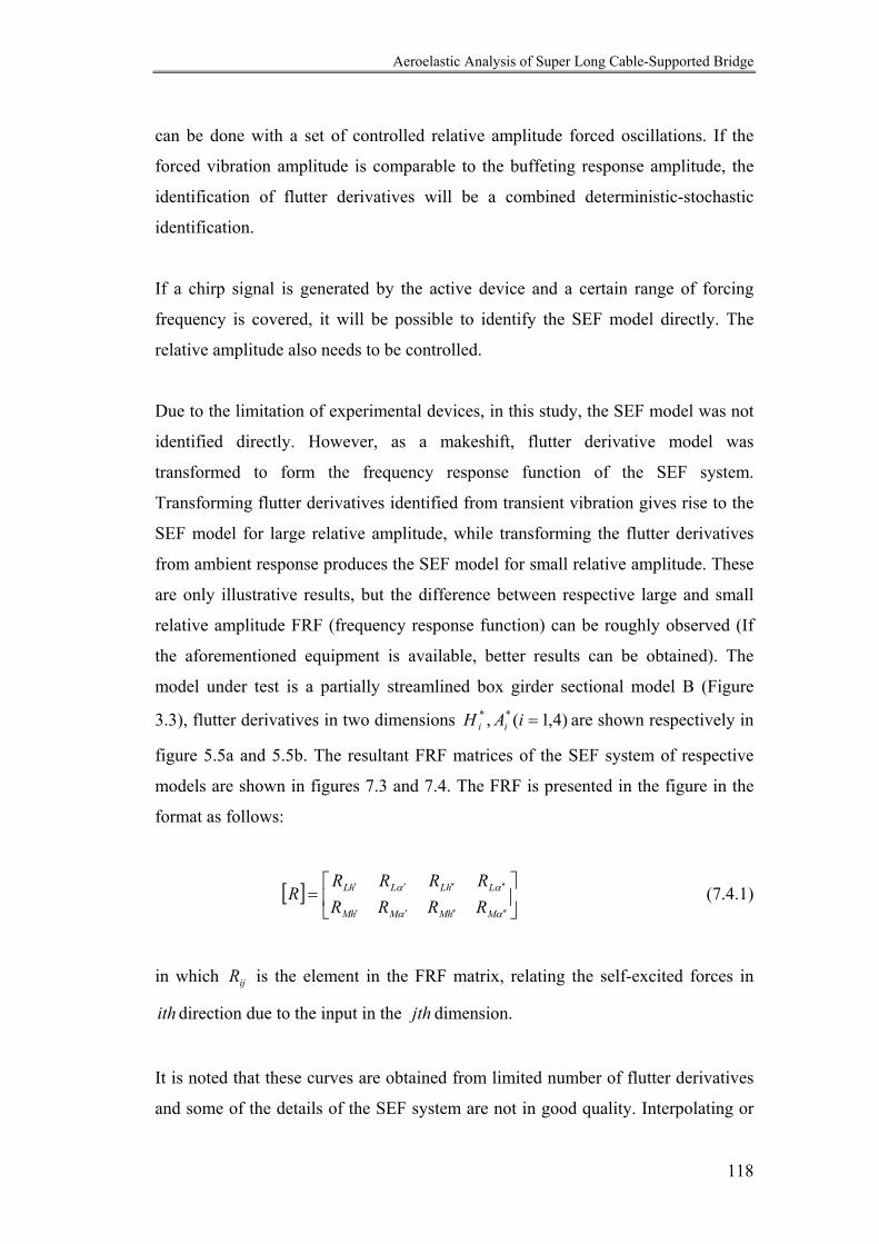
Aeroelastic Analysis of Super Long Cable-Supported Bridge
118
can be done with a set of controlled relative amplitude forced oscillations. If the
forced vibration amplitude is comparable to the buffeting response amplitude, the
identification of flutter derivatives will be a combined deterministic-stochastic
identification.
If a chirp signal is generated by the active device and a certain range of forcing
frequency is covered, it will be possible to identify the SEF model directly. The
relative amplitude also needs to be controlled.
Due to the limitation of experimental devices, in this study, the SEF model was not
identified directly. However, as a makeshift, flutter derivative model was
transformed to form the frequency response function of the SEF system.
Transforming flutter derivatives identified from transient vibration gives rise to the
SEF model for large relative amplitude, while transforming the flutter derivatives
from ambient response produces the SEF model for small relative amplitude. These
are only illustrative results, but the difference between respective large and small
relative amplitude FRF (frequency response function) can be roughly observed (If
the aforementioned equipment is available, better results can be obtained). The
model under test is a partially streamlined box girder sectional model B (Figure
3.3), flutter derivatives in two dimensions )4,1(, ** =iAH ii are shown respectively in
figure 5.5a and 5.5b. The resultant FRF matrices of the SEF system of respective
models are shown in figures 7.3 and 7.4. The FRF is presented in the figure in the
format as follows:
[ ]
=
′′′′′′
′′′′′′
αα
αα
MhMMhM
LhLLhL
RRRRRRRR
R (7.4.1)
in which ijR is the element in the FRF matrix, relating the self-excited forces in
ith direction due to the input in the jth dimension.
It is noted that these curves are obtained from limited number of flutter derivatives
and some of the details of the SEF system are not in good quality. Interpolating or
Aeroelastic Analysis of Super Long Cable-Supported Bridge
119
extrapolating the result will not improve the reliability of the identification,
therefore they are not suitable for the identification of the SEF model and direct
measurement mentioned above is needed.
Another issue regarding the FRF matrix so measured is that it is real. This is due to
the fact that the flutter derivative matrix [ ]Η and state matrix [ ]fsA are both real.
Identifying FRF of SEF from flutter derivative matrix is equivalent to finding a
matrix [ ]Φ , mapping the time history of rigid body state vector multiplied by the
flutter derivative matrix to weighted integration of its dimensionless time
derivative. The weighting function in this case is the impulse response function of
SEF system. Therefore, the calculated FRF is real. If the FRF of SEF is measured
directly, it is not necessary to be a real matrix.
Summary
Linear SEF dynamic system model for self-excited forces on bridge deck is
presented, making it possible to study the relative amplitude effect in more detail.
Direct experimental determination of the of SEF generation system in time domain
is possible if SEF model is adopted. To measure the FRF and further identify the
time domain representation of the SEF system, a new experimental method is
suggested but not exercised due to the limitation of equipment. SEF model may
serve as a more general formulation of self-excited forces.
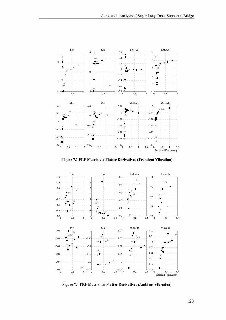
Aeroelastic Analysis of Super Long Cable-Supported Bridge
120
0 0.5 1-3
-2
-1
0
1L-h
0 0.5 1-5
0
5L-a
0 0.5 1-0.8
-0.6
-0.4
-0.2
0
0.2
0.4
0.6L-dh/ds
0 0.5 1-4
-3
-2
-1
0
1L-da/ds
0 0.5 1 1.5-0.3
-0.2
-0.1
0
0.1
0.2M-h
0 0.5 1 1.5-0.15
-0.1
-0.05
0
0.05M-a
0 0.5 1 1.5-0.05
-0.04
-0.03
-0.02
-0.01
0
0.01M-dh/ds
0 0.5 1 1.5-0.06
-0.05
-0.04
-0.03
-0.02
-0.01
0
Reduced Frequency
M-da/ds
Figure 7.3 FRF Matrix via Flutter Derivatives (Transient Vibration)
0 0.2 0.4-1.8
-1.6
-1.4
-1.2
-1
-0.8
-0.6
-0.4L-h
0 0.2 0.4-2
-1
0
1
2
3
4
5L-a
0 0.2 0.4-0.8
-0.7
-0.6
-0.5
-0.4
-0.3L-dh/ds
0 0.2 0.4-0.8
-0.6
-0.4
-0.2
0L-da/ds
0 0.2 0.4-0.08
-0.07
-0.06
-0.05
-0.04
-0.03M-h
0 0.2 0.4-0.25
-0.2
-0.15
-0.1
-0.05
0M-a
0 0.2 0.4-0.01
0
0.01
0.02
0.03
0.04M-dh/ds
0 0.2 0.4-0.05
-0.04
-0.03
-0.02
-0.01
0
0.01
0.02
Reduced Frequency
M-da/ds
Figure 7.4 FRF Matrix via Flutter Derivatives (Ambient Vibration)
Aeroelastic Analysis of Super Long Cable-Supported Bridge
121
CHAPTER EIGHT
Errors in the Identification of
Aeroelastic Derivatives
Abstract:
Errors in the identification of flutter derivatives may be due to nonlinearity in the
aeroelastic system as indicated by the relative amplitude effect, possible strong
wake oscillator behind the body or poor experimental conditions such as the high
level noise in the identified Markov parameters. In this chapter, error indices are
used as a confidence indicator of the identification. These indices are built on the
instantaneous energy discrepancy between the identified and the measured system
in subspace, and the real values of flutter derivatives are not needed during the
evaluation. The discussion is within the framework of eigensystem realization
algorithm (ERA).

Aeroelastic Analysis of Super Long Cable-Supported Bridge
122
8.1 Introduction:
There are some error sources in the identification of flutter derivative model such as
the nonlinearity in the self-excited wind force as indicated by the relative amplitude
effect, noise in the measurement, non-whiteness of the buffeting force (Bogunovic-
Jacobsen 1995) and so on.
8.1.1 Errors due to Non-White Noise
The experiments with ambient response might be sensitive to the nature of the
external excitations since the model is totally “noise driven” in this case. An
identification method based on response data only cannot distinguish between the
properties belonging to the structure or the load. The nonwhite noise in the system
can be attributed to at least the two factors listed below.
8.1.1.1 Non-White Noise Due to the Fluid Oscillation
The time-frequency domain hybrid linear model using flutter derivatives has always
been dissociated from those bridge deck forms that exhibit strong vortex-shedding
effects and lock-in in certain velocity ranges. In other words, at an earlier stage
either some bluff deck forms prone to vortex excitation are deemed to be entirely
untreatable by flutter derivative methods or the application of these method was
provisionally suspended over strong vortex shedding lock in velocity regimes.
Bogunovic-Jakobsen (1995) discussed the effect of non-white noise effects of the
buffeting wind load on the identification of aeroelastic derivatives. The power
spectral density of wind load on a stationary sectional model is needed to create a
filter to correct the measured data. One possible disadvantage is that buffeting load
is measured in a separate experiment. Putting together two experiments possibly
under different conditions might not be an acceptable way to evaluate the result of

Aeroelastic Analysis of Super Long Cable-Supported Bridge
123
the identification. This method also leads to difficulties when the DOF of the
system is more than one.
8.1.1.2 Non-White Noise Due to Structural Vibration.
The other source of non-whiteness in the input is due to the additional vibration
source in the suspension system. If we expand the order of the state space model
for the aeroelastic system to include this part of vibration, the state vector is
expressed as
TTs
Tm tXtXtX )()()( = (8.1.1)
In the state vector, mX is the rigid body degree of freedom (DOF), if the
experiment is 3D, its dimension, mDim , is six, sX is DOF due to other vibration
sources, its dimension, sDim , is unknown. If the suspension system is not strong
enough the measurement could possibly contain other sources of vibration, such as
the ground vibration or the suspension system vibration and so on.
The corresponding state space equation will be
buffBftAXtX += )()(&
)()( tCXtY = (8.1.2)
in which A is the state matrix, having dimension
( ) ( )ssA DimDimDim +×+= 66 , (8.1.3)
Matrix B is the input matrix for random buffeting load and
Matrix C is the output matrix, having dimension
Aeroelastic Analysis of Super Long Cable-Supported Bridge
124
)6(3 sC DimDim +×= . (8.1.4)
The column vector )(tY is the output vector at time t . Since only the rigid body
motion is measured, the dimension of the output vector remains unchanged.
However, our goal is not to identify this model of unknown order, but rather, unlike
other situations in which system identification is used, to identify a system that has
a fixed order, i.e. the state matrix A , in 3 DOF experiment, must have order 6.
However, in the experiment, it is not necessarily true that the signal measured
carries nothing else but the desired information. Other sources of vibration can also
be represented. The vibration of the suspension system and other vibration sources
could affect the pre-assumption that the signal has an order of 6. By truncating the
system to order six, the originally internal forces between the truncated degrees of
freedom and the remaining ones become external, and may contribute to the non-
white component of the unknown buffeting force.
8.1.2 Errors Due To Nonlinearity in the Self-Excited Forces
It is difficult, however, to attribute the errors in the identification of flutter
derivatives solely to the nonwhite noise effect, since the argument above is as weak
as either the fluid states of the aeroelastic system or the additional structural states
of the suspension system. The major errors come from, at least in the experiment
described in the thesis, the non-stationary nature of the triggered free decay
vibration.
The study in previous chapters indicates that the relative amplitude has a notable
effect on the identified flutter derivatives. Flutter derivatives identified under the
conditions of small and large relative amplitude may be different. In transient
vibration tests, the triggered vibration is clearly larger than the ambient vibration at
the beginning, but decays very fast into the ambient vibration envelope. When the
vibration starts, the relative amplitude effect is negligible but it is not at the end.
Aeroelastic Analysis of Super Long Cable-Supported Bridge
125
The identification of flutter derivatives corresponding to the free decay vibration
actually deals with a time-varying phenomenon. On the contrary, in the experiment
with ambient vibration, there is no change in the relative amplitude because the
impulse response is calculated numerically by output covariance. The phenomenon
to be identified is time-invariant under this condition.
As in these two cases of the identification of free decay and ambient vibration, other
factors remain almost the same; it is predictable that if the identification errors in
the former case are considerably larger than those in the latter case, the transient
nature of the free decay vibration may be considered to have a contribution to errors
in the identification. The remaining part of the chapter will serve as a proof.
8.2 Evaluation Based on Block Hankel Matrix
Based on the analysis in the previous part, it is necessary to present an index of
confidence together with the identified flutter derivatives. It is straightforward to
create a ratio of the signal power of the rigid body to the signal power of the cut off
parts in the Block Hankel Matrix.
By the fundamental ideas of ERA (Juang, 1994), The measured Block Hankel
Matrix is decomposed with SVD
[ ] [ ]Tnn
n SSPPH 00
0 00
)0(ˆ
Σ
Σ= (8.2.1)
[ ] Nn PPP ≡0 and [ ] Nn SSS ≡0 are orthogonal, and eigenvector matrices of
)0(ˆ)0(ˆ HH T and )0(ˆ)0(ˆ THH , respectively. nΣ and 0Σ are diagonal matrices, their
elements are positive singular values. Their magnitudes reflect the contribution of
the signal in that dimension to the overall measurements. The dimensions of
nΣ equal the order of the state-space model. Elements in 0Σ are small and
considered negligible. If the measured Hankel matrix is exactly generated by a
Aeroelastic Analysis of Super Long Cable-Supported Bridge
126
linear time invariant system, elements in 0Σ are exactly zero. Due to the
incompleteness of the flutter derivative model and other error sources 0Σ might not
be small, but deemed as zero in the identification.
Because the ERA interprets singular vectors as directions in the system, in the
evaluation of errors in the identification, it is needed to find a common coordinate,
onto which both realized and unrealized parts are projected. By such projection, the
“realized signal ellipsoid” and “unrealized signal ellipsoid” can be constructed. The
length of each semi-axis of the ellipsoids can quantify the contribution of the signal
to the overall Block Hankel Matrix in each direction defined by the projection
matrix. The power corresponding to each direction can be compared without
confusing the dimensions the signal powers correspond to.
By observation, the matrix [ ]0PPn is a good candidate for the aforementioned
base matrix.
Projecting the Block Hankel Matrix to the subspace TnP we have )0(HPT
n . We
define the realized signal power matrix on the subspace TnP of the defined base
matrix as
nTT
n PHHP )0()0(=Θ . (8.2.3)
It is clear that the signal power matrix so defined is symmetric and positive semi-
definite. The singular values of the signal power matrix Θ equal to its eigenvalues,
i.e.
TQQD 2=Θ (8.2.4)
where ),,,( 21 nddddiagD L= , 2id is the eigenvalue as well as singular values of
signal power matrix Θ . Hence the singular values define the length of semi-axes of
Aeroelastic Analysis of Super Long Cable-Supported Bridge
127
the signal ellipsoid, while the column vectors of the orthogonal matrix Q define the
directions of these axes.
The error signal matrix is defined as
−=−
=
)0(ˆˆ
)0(ˆ0
)0()(
0 HPNPHP
HPnE
T
TnT
N
Tn
r (8.2.5)
in which ][ 0PPP nN = is the orthogonal projection matrix; )0(ˆ)0(ˆ HHN −= is
the error matrix between the identified block Hankel matrix )0(H and the
originally measured block Hankel matrix )0(H in the original coordinate.
The power matrix of the error signal is defined as:
==
Ξ
Ξ
002
1
)0(ˆ)0(ˆ00ˆˆ
)()(0
0PHHP
PNNPnEnETT
nTT
nTrr . (8.2.6)
The first part is the projection of the difference between the measured and identified
Block Hankel Matrix in the direction of the identified singular vectors TnP . The
second part is projection of the measured Block Hankel Matrix on the unidentified
part of the singular vector TP0 , the orthogonal complement of TnP . Because of the
truncation of singular values, and singular vectors, the SVD of the identified Block
Hankel Matrix does not produce TP0 and the subspace formed by TP0 is not a part of
)0(H . The projection of )0(H onto these directions are zero, so only )0(H is
considered in projecting onto TP0 .
The 1Ξ part is the error due to the computation, which will be shown, in the
following result, is small.

Aeroelastic Analysis of Super Long Cable-Supported Bridge
128
It is clear that energy of 2Ξ belongs to the directions that are not a part of the
aeroelastically influenced rigid body motion. Within the structure of ERA, it is
excluded from the system and cannot be incorporated into the rigid body motion
direction, unless additional states are included. If this part of energy is unacceptably
large, the identification may cease to be effective to represent the behavior of the
deck.
Define the sum of all semi-axes of the signal ellipsoid as the overall power in the
subspace defined by the semi-axes. The trace of the matrix Θ or Ξ produces the
sum of the eigenvalues and, in this case, the sum of singular values as well. Hence
we have the summation of realized power in the rigid body motion direction of the
state space
∑=
=Θn
ii
TTi pHHpTr
1)0()0()( . (8.2.7)
The summary of error power in the rigid body motion direction of the state space is
∑=
=Ξn
ii
TTi pNNpTr
11
ˆˆ)( , (8.2.8)
in other directions
∑+=
=ΞN
njj
TTj pHHpTr
12 )0(ˆ)0(ˆ)( . (8.2.9)
We have two ratio values: the ratio of error to signal power in the rigid body motion
direction:
)()( 1
1 ΘΞ
=ΩTrTr
(8.2.10)
and in other directions
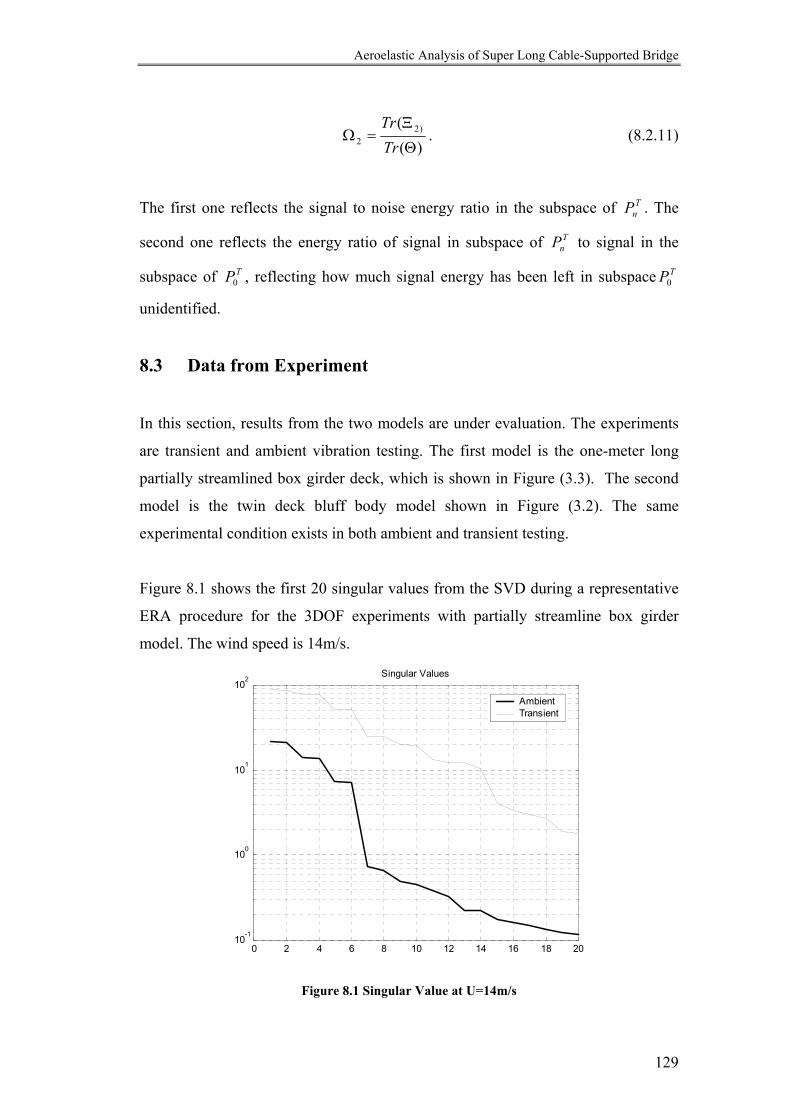
Aeroelastic Analysis of Super Long Cable-Supported Bridge
129
)(( )2
2 Θ
Ξ=Ω
TrTr
. (8.2.11)
The first one reflects the signal to noise energy ratio in the subspace of TnP . The
second one reflects the energy ratio of signal in subspace of TnP to signal in the
subspace of TP0 , reflecting how much signal energy has been left in subspace TP0
unidentified.
8.3 Data from Experiment
In this section, results from the two models are under evaluation. The experiments
are transient and ambient vibration testing. The first model is the one-meter long
partially streamlined box girder deck, which is shown in Figure (3.3). The second
model is the twin deck bluff body model shown in Figure (3.2). The same
experimental condition exists in both ambient and transient testing.
Figure 8.1 shows the first 20 singular values from the SVD during a representative
ERA procedure for the 3DOF experiments with partially streamline box girder
model. The wind speed is 14m/s.
0 2 4 6 8 10 12 14 16 18 2010
-1
100
101
102
Singular Values
Ambient Transient
Figure 8.1 Singular Value at U=14m/s
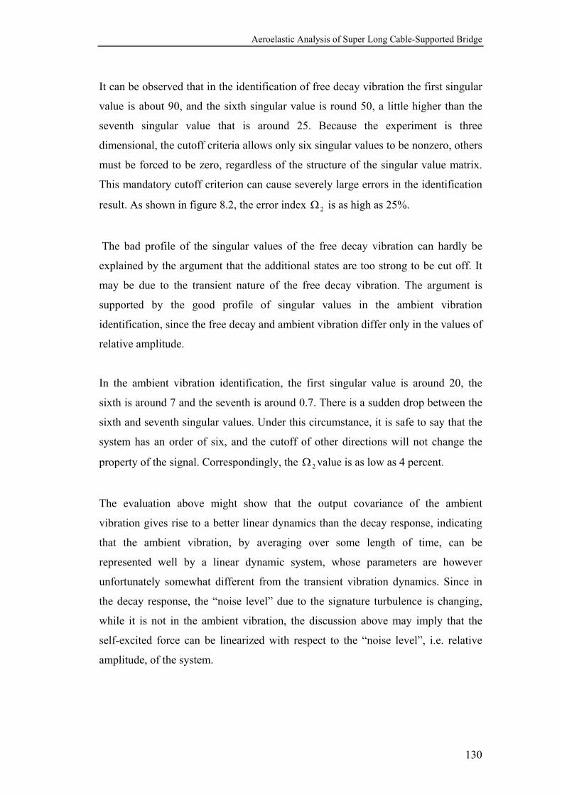
Aeroelastic Analysis of Super Long Cable-Supported Bridge
130
It can be observed that in the identification of free decay vibration the first singular
value is about 90, and the sixth singular value is round 50, a little higher than the
seventh singular value that is around 25. Because the experiment is three
dimensional, the cutoff criteria allows only six singular values to be nonzero, others
must be forced to be zero, regardless of the structure of the singular value matrix.
This mandatory cutoff criterion can cause severely large errors in the identification
result. As shown in figure 8.2, the error index 2Ω is as high as 25%.
The bad profile of the singular values of the free decay vibration can hardly be
explained by the argument that the additional states are too strong to be cut off. It
may be due to the transient nature of the free decay vibration. The argument is
supported by the good profile of singular values in the ambient vibration
identification, since the free decay and ambient vibration differ only in the values of
relative amplitude.
In the ambient vibration identification, the first singular value is around 20, the
sixth is around 7 and the seventh is around 0.7. There is a sudden drop between the
sixth and seventh singular values. Under this circumstance, it is safe to say that the
system has an order of six, and the cutoff of other directions will not change the
property of the signal. Correspondingly, the 2Ω value is as low as 4 percent.
The evaluation above might show that the output covariance of the ambient
vibration gives rise to a better linear dynamics than the decay response, indicating
that the ambient vibration, by averaging over some length of time, can be
represented well by a linear dynamic system, whose parameters are however
unfortunately somewhat different from the transient vibration dynamics. Since in
the decay response, the “noise level” due to the signature turbulence is changing,
while it is not in the ambient vibration, the discussion above may imply that the
self-excited force can be linearized with respect to the “noise level”, i.e. relative
amplitude, of the system.
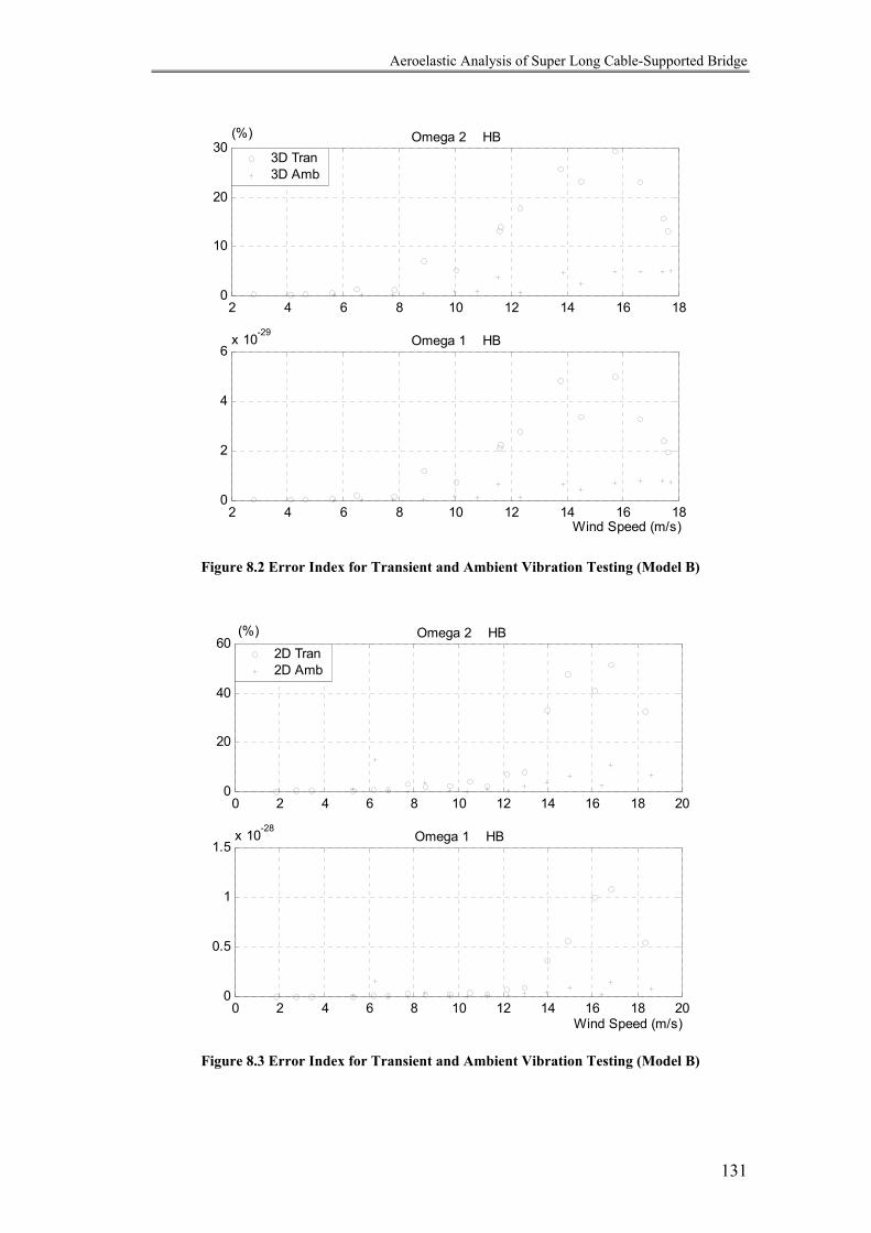
Aeroelastic Analysis of Super Long Cable-Supported Bridge
131
2 4 6 8 10 12 14 16 180
2
4
6x 10-29
2 4 6 8 10 12 14 16 180
10
20
303D Tran3D Amb
Omega 2 HB
Omega 1 HB
(%)
Wind Speed (m/s)
Figure 8.2 Error Index for Transient and Ambient Vibration Testing (Model B)
0 2 4 6 8 10 12 14 16 18 200
0.5
1
1.5x 10⁻²⁸
0 2 4 6 8 10 12 14 16 18 200
20
40
602D Tran2D Amb
Omega 2 HB
Omega 1 HB
Wind Speed (m/s)
(%)
Figure 8.3 Error Index for Transient and Ambient Vibration Testing (Model B)
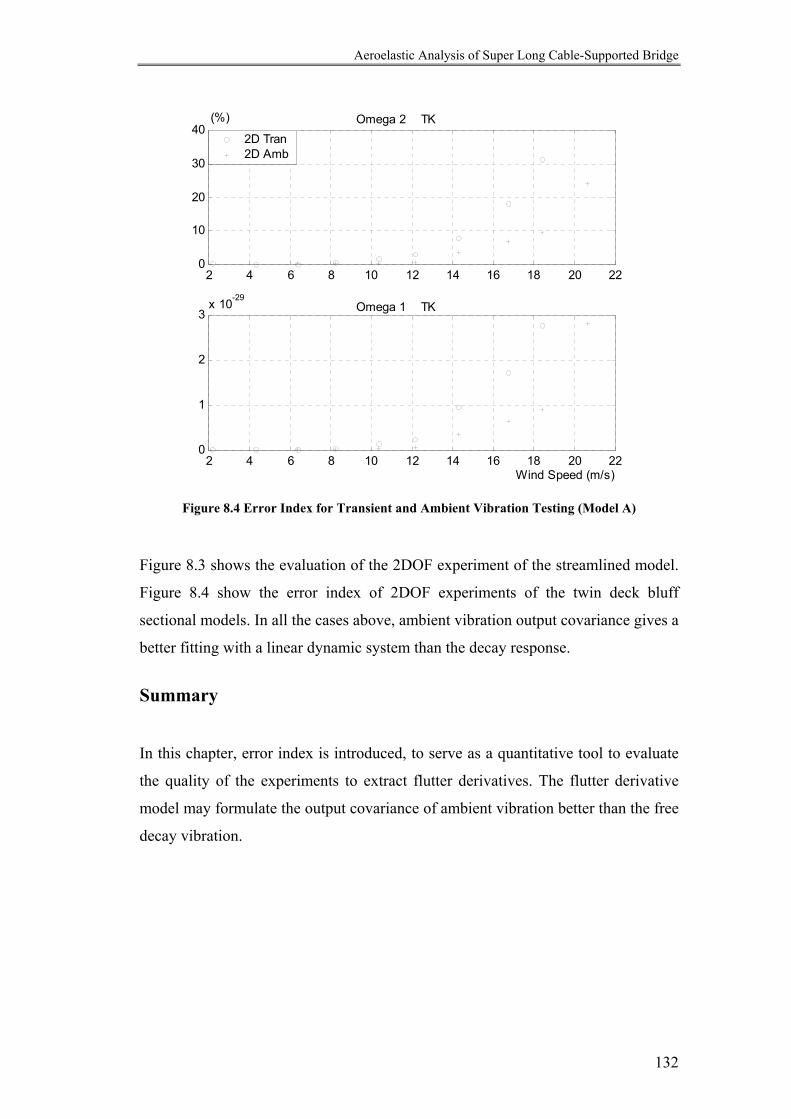
Aeroelastic Analysis of Super Long Cable-Supported Bridge
132
2 4 6 8 10 12 14 16 18 20 220
1
2
3x 10-29
2 4 6 8 10 12 14 16 18 20 220
10
20
30
402D Tran2D Amb
Omega 2 TK
Omega 1 TK
Wind Speed (m/s)
(%)
Figure 8.4 Error Index for Transient and Ambient Vibration Testing (Model A)
Figure 8.3 shows the evaluation of the 2DOF experiment of the streamlined model.
Figure 8.4 show the error index of 2DOF experiments of the twin deck bluff
sectional models. In all the cases above, ambient vibration output covariance gives a
better fitting with a linear dynamic system than the decay response.
Summary
In this chapter, error index is introduced, to serve as a quantitative tool to evaluate
the quality of the experiments to extract flutter derivatives. The flutter derivative
model may formulate the output covariance of ambient vibration better than the free
decay vibration.
Aeroelastic Analysis of Super Long Cable-Supported Bridge
133
CHAPTER NINE
Conclusions and Future Work
9.1 Conclusions
The research described herein consists of studies on properties of interactive wind
forces on elastically supported bluff bridge sectional models. Two and three-
dimensional sectional model tests in a wind tunnel were carried out to detect the
nonlinearity in the self-excited wind forces. This work is needed because the
transformation of frequency-time domain hybrid flutter derivative model to either
time or frequency domain usually requires the linearity assumption of the self-
excited wind forces, which has not been investigated thoroughly.
In this study,
1: Nonlinearity in self-excited wind forces was detected through the concept of
relative amplitude of the aeroelastically-influenced system.

Aeroelastic Analysis of Super Long Cable-Supported Bridge
134
This method is different from the usual practice of examining the amplitude
effect on flutter derivative. Because aeroelastic analysis is by and large
meant to predict the structural behavior when the structural vibration
amplitude and the angle of attack of the oncoming wind are both small, it is
important to detect the existence of nonlinearity in the self-excited force
under the same condition.
Relative amplitude is defined as the body oscillatory amplitude relative to
the ambient vibration envelope. It reflects the relation between the
mechanically triggered body oscillations and aerodynamically induced
random vibration due to turbulence, indicating the relative importance of the
two factors. Physically, the larger the buffeting component in the total
response, the more the information about the fluid feature than about the
structure the system carries, and vice versa. These two conditions are
different in that the body oscillation may change the behavior of the
surrounding fluid if its amplitude exceeds the ambient vibration amplitude,
and the identified flutter derivatives may also be changed.
Ambient vibration and triggered free decay vibration are two extreme cases
of the tests on the relative amplitude effect. By comparing resultant flutter
derivatives of these two extreme cases, the nonlinearity is detected.
The effect of relative amplitude on flutter derivatives and on the flutter
boundary reveals, from the structural point of view, a complex relationship
between the self-excited forces and the “structural vibration noise” due to
signature turbulence related buffeting forces. Although the aeroelastic forces
are linear when the body motion due to an external trigger is not affected
significantly by the signature turbulence, they are nonlinear when the noise
component in the vibration due to the signature turbulence related buffeting
forces could not be neglected.

Aeroelastic Analysis of Super Long Cable-Supported Bridge
135
2: By using flutter derivatives of a partially streamlined box girder section
identified form transient and ambient vibration testing, the relative
amplitude effect on flutter instability is studied.
The flutter derivatives from ambient vibration were found aeroelastically
stable. Therefore, the relative amplitude effect has a stabilizing
consequence. The relative amplitude effect may also be used to study the
turbulence effect on flutter, but further studies are needed.
3: The effect of lateral flutter derivatives was investigated by using 3DOF and
2DOF flutter derivatives.
In comparison with the two cases where flutter derivatives used are 2D or
3D, the analysis with 3D flutter derivatives with P related flutter derivatives
being assigned zero gives rise to the lowest flutter wind speed. The 2D
flutter derivatives produce the highest wind speed for instability. Both in the
two cases of 2D and 3D with P derivatives assigned zero, two flutter
conditions were found within the reduced velocity range covered by
experiments producing two flutter frequencies and modes in both cases.
Only one flutter condition was found in the 3D case. It corresponds to the
higher second flutter mode in the other analytical cases. The lower flutter
mode is “pushed”, by the P derivatives, outside the reduced velocity range
covered by experiment
All these discussions are limited to the specific section type under study.
Because the experimental result is not in consistence with that from quasi-
static theory, the conclusion of the investigation is somewhat different from
the usual idea based on the quasi-static theory.
4: A more general formulation of self-excited wind forces is discussed.
The formulation in time domain of the self-exited force on bridge decks
often employs indicial function by transforming the flutter derivative model.
Aeroelastic Analysis of Super Long Cable-Supported Bridge
136
However the relative amplitude effect may make the transformation
questionable if the flutter derivatives identified from transient and ambient
vibration are different.
As it is suspected in this study that the self-excited wind forces might be
linearized with respect to the relative amplitude, an alternative model
treating the self-exited force generation mechanism as a separate dynamic
system may be favorable to offer more flexibilities in manipulating the
sectional model testing.
In this paper, SEF generation system coupled with the rigid bridge deck
system is proposed. This expression was linked to the frequency-time
domain hybrid form of flutter derivative model and transform relationship
between the two models was also suggested. The SEF model enables the
treatment of the self-exited forces as an independent dynamic system and
direct identification in time domain.
5: One of the error sources in extracting flutter derivatives was identified.
The ineffectiveness of the identification of flutter derivatives may be due to
nonlinearity in the aeroelastic system as has been indicated by the relative
amplitude effect, possible strong wake oscillator behind the body or poor
experimental conditions such as the high level noise in the identified
Markov parameters.
As all factors remain almost the same in the two cases of the identification
of free decay and ambient vibration, it is predictable that if the identification
errors in the former case are considerably larger than those in the latter case,
the non-stationary nature of the free decay vibration will contribute to errors
in the identification.
The evaluation might suggest that the output covariance of the ambient
vibration gives rise to a better linear dynamics than the decay response does.
Aeroelastic Analysis of Super Long Cable-Supported Bridge
137
This indicates that the ambient vibration, by averaging over some length of
time, can be represented by a linear dynamic system, whose parameters are
however unfortunately somewhat different from the transient vibration
dynamics. It is noticed that in the decay response, the “noise” level due to
the turbulence is changing, while it is not in the ambient vibration. This
might imply that the self-excited force can be linearized with respect to the
noise level in the system.
9.2 Suggestions for Future Work
Studies on the formulation of interactive wind forces on bridge decks are far from
ending. It must be recognized that the frequency-time domain hybrid flutter
derivative model works under specific conditions. Any transformation of the model
will only extend it nominally. The surplus information so generated may be
factious. To formulate the self-excited force for more general purpose, conceptual
models for experiments that can work in time domain are needed. The following
subjects are among the most important:
1: Criteria evaluating the quality of transforming the flutter derivative model to
time domain.
2: Nonlinear model in time domain for the self-excited wind force.
3: Nonlinear identification method to identify the aeroelastically influenced
model directly.
Therefore, in order to have better approaches for flutter and buffeting analysis, it is
important to have a better understanding of the self-excited forces.
138
Appendix I Output Covariance of Discrete-Time State Space System (Overschee and Moor 1996)
When the measurement noise in the equipment and process noise (the small scale
buffeting force due to signature turbulence and local variation of wind speed in the
oncoming flow) is white and zero mean, then
0][ =⋅ TqXE and 0][ =⋅ TwXE (5.A.1)
where )()( iBpiq = and )()( iDviw = .
The Lyapunov equation for the state covariance matrix is
QAAiXiXE Tsi
Tsi +Σ=+⋅+=Σ + )]1()1([1 (5.A.2)
where )]()([ iqiqEQ T⋅= .
If output covariance is defined as
)]()([)( iYkiYEkC Ti ⋅+= (5.A.3)
then
RCCiYiYEC Tsi
Ti +Σ=⋅= )]()([)0( (5.A.4)
where )]()([ iwiwER T⋅= .
If we define
SCAiYiXEG Tsi
T +Σ=⋅+= )]()1([ , (5.A.5)
where )]()([ iwiqES ⋅= , we have for L,2,1=k
GCAkC ki
1)( −= . (5.A.6)
This produces a new state-space model of )0(,,, iCCGA .
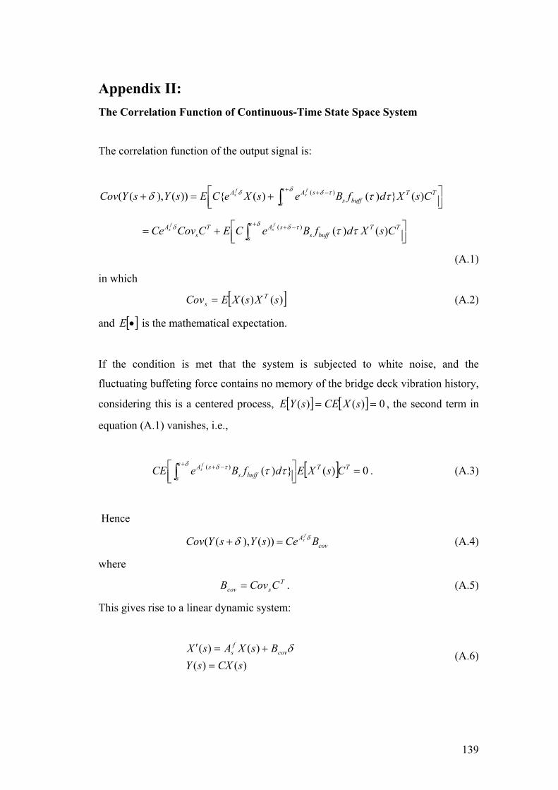
139
Appendix II: The Correlation Function of Continuous-Time State Space System
The correlation function of the output signal is:
+=+ ∫
+ −+δ τδδ ττδs
s
TTbuffs
sAA CsXdfBesXeCEsYsYCovfs
fs )()()())(),(( )(
+= ∫
+ −+δ τδδ ττs
s
TTbuffs
sATs
A CsXdfBeCECCovCefs
fs )()()(
(A.1)
in which
[ ])()( sXsXECov Ts = (A.2)
and [ ]•E is the mathematical expectation.
If the condition is met that the system is subjected to white noise, and the
fluctuating buffeting force contains no memory of the bridge deck vibration history,
considering this is a centered process, [ ] [ ] 0)()( == sXCEsYE , the second term in
equation (A.1) vanishes, i.e.,
[ ] 0)()()( =
∫
+ −+ TTs
s buffssA CsXEdfBeCE
fs
δ τδ ττ . (A.3)
Hence
covA BCesYsYCovfs δδ =+ ))(),(( (A.4)
where T
scov CCovB = . (A.5)
This gives rise to a linear dynamic system:
)()()()(
sCXsYBsXAsX cov
fs
=+=′ δ
(A.6)
140
Reference
Afolabi, D. (1994)
Flutter Analysis Using Transversality Theory
Acta Mechanica 103 p1-15
Afolabi, D. (1995)
Sylvester’s Eliminant and Stability Criteria for Gyroscopic Systems
Journal of Sound and Vibration 182(2) p229-244
Afolabi, D. and Pidaparti, R.M.V. (1998)
Flutter Prediction Using an Eigenvector Orientation Approach
AIAA Journal, Vol. 36 No. 1, p69-74
Agar, T. T.A. (1988)
The Analysis of Aerodynamic Flutter of Suspension Bridges
Computers and Structures, 30, p593-600
Agar, T. T. A. (1989)
Aerodynamic Flutter Analysis of Suspension Bridges by a Modal Technique
Engineering Structures, 11, p75-82
Arnold, V.I. (1971)
On Matrices Depending on Parameters
Russian Math. Surveys 26, p29-43
Astiz, M. A. (1998)
Flutter Stability of Very Long Suspension Bridges
Journal of Bridge Engineering, ASCE, Vol. 3, No. 3, p132-139
Bay, J.S. (1998)
Fundamentals of Linear State Space Systems
141
Mcgraw-Hill Companies, Inc.
Bienkiewicz, B and Kobayashi, H (1993)
Effects of Partial Streamlining on Aerodynamic Response of Bridge Decks
Journal of Structural Engineering, ASCE, Vol. 119, No. 1, p342-348
Bihop, R. E. D., and Hassan, A. Y. (1964)
The Lift and Drag Forces on a Circular Cylinder in a Flowing Field.
Proc. Roy. Soc.(London) Ser. A, 277, p51-75
Bisplinghoff, R. L., and Ashley, H. (1962)
Principle of Aeroelasticity,
John Wiley And Sons, Inc., New York, N. Y.
Blevins, R. D. (1977)
Flow-Induced Vibration
Van Nostrand Reinhold Company
Bogunovic-Jakobsen, J. (1995)
Fluctuating Wind Load and Response of a Line-Like Engineering Structure With
Emphasis on Motion-Induced Wind Forces
Doktor Ingenioravhandling, 1995:62
Institutt for Konstruksjonsteknikk Trondheim
Boonyapinyo, V.; Yamada, H. and Miyata, T (1994)
Wind-Induced Nonlinear Lateral-Torsional Buckling of Cable Stayed Bridges
Journal of Structural Engineering, ASCE, Vol. 120, No.2, p486-506
Boonyapinyo, V.; Miyata, T. and Yamada, H. (1999)
Advanced Aerodynamic Analysis of Suspension Bridges by State-Space Approach
Journal of Structural Engineering, ASCE, Vol. 125, No.12, p1357-1366

142
Brownjohn, J.M.W; Dumanoglu, A.A.; Severn, R.T and Taylor, C.A. (1987)
Ambient Measurements of the Humber Suspension Bridge and Comparison with
Calculated Characteristics
Proceedings of Institution of Civil Engineers Part 2, 1987, 83, Sept., p561-600
Brownjohn, J.M.W. (1990)
Humber Bridge Monitoring Digital Measurements March-May 1990 and
Preliminary Analysis
Report UBCE_EE_90_10, Department Of Civil Engineering, University Of Bristol.
Brownjohn, J.M.W.; Zasso, A; Stephen, G.A. and Severn, P.T. (1995)
Analysis of Experimental Data from Wind Induced Response of a Long Span
Bridge
Journal of Wind Engineering and Industrial Aerodynamics, 54/55 (1995) p13-24
Brownjohn, J.M.W and Xia, P. (1999)
Finite Element Updating of a Damaged Structure
Proceedings, IMAC 17, Vol. 1, Florida USA, Feb. 1999, p457-462
Brownjohn, J.M.W. and Choi, C.C. (2001)
Wind Tunnel Section Model Study of Aeroelastic Performance for Ting Kau Bridge
Deck
Wind & Structures, an international Journal, Vol. 4, No.5 (2001) p367-382
Bucher, C. G., and Lin, Y. K. (1988).
Stochastic Stability of Bridges Considering Coupled Modes: I.
Journal of Engineering Mechanics, ASCE, 114(12) p2055-2070
Bucher, C. G., and Lin, Y. K. (1989).
Stochastic Stability of Bridges Considering Coupled Modes: II.
Journal of Engineering Mechanics, ASCE, 115(2) p384-400

143
Cai, C. S.; Albrecht, P. and Bosch, H. R. (1999)
Flutter and Buffeting Analysis I: Finite Element and RPE Solution.
Journal of Bridge Engineering, ASCE, 4(3) p174-180
Cai, C. S., Albrecht, P., and Bosch, H. R. (1999)
Flutter and Buffeting Analysis. II: Luling and Deer Isle Bridges.
Journal of Bridge Engineering, ASCE, 4(3) p174-180
Chen, X. Z., Matsumoto, M. and Kareem, A. (2000 A)
Time Domain Flutter and Buffeting Response Analysis of Bridges
Journal of Engineering Mechanics, ASCE, Vol. 126 No.1 p7-16
Chen, X. Z., Matsumoto, M. and Kareem, A. (2000 B)
Aerodynamic Coupling Effects on Flutter and Buffeting of Bridges
Journal of Engineering Mechanics, ASCE, Vol. 126 No.1, p17-26
Davenport, A.G.
Comparison of Model and Full-Scale Tests on Bridges
(Sources Not Clear)
Davenport, A.G. (1962)
The Buffeting of a Suspension Bridge by Storm Winds
Journal of Structural Division, ASCE, Vol. 88, p 233-268
Davenport, A.G. (1998)
Probabilistic Method in Wind Engineering for Long Span Bridges
Bridge Aerodynamics, Larsen and Esdahl (eds), Balkema, Rotterdam
Davenport, A.G.; King, J.P.C. and Larose, G.L. (1992)
Taut Strip Model Testing
Proc., Int. Symp. on Aerodynamics of Large Bridges, Larsen A. (ed),
Balkema, Rotterdam, The Netherlands. p113-124
144
Diana,G.; Cheli, F and Resta,F. (1995)
Time Domain Aeroelastic Force Identification on Bridge Decks
9ICWE New Delhi, India
Diana, G., Bruni, S., Collina, A., and Zasso, A. (1998)
Aerodynamic Challenges in Super Long Span Bridges Design
Bridge Aerodynamics, Larsen and Esdahl, ed, p131-144
Ding, Q. and Lee, P.K.K (2000)
Computer Simulation of Buffeting Actions of Suspension Bridge under Turbulent
Wind
Computers and Structures 76(2000) p787-797
Dung, N. N.; Miyata, T and Yamada, H; (1996)
The Mode Tracing Method for Flutter of Long Span Bridges
Proceedings of the 14th National Symposium on Wind Engineering, Kyoto, Japan
Dung, N. N.; Miyata, T.; Yamada, H.; and Minh, N. N. (1998)
Flutter Responses in Long Span Bridges with Wind Induced Displacement by the
Mode Tracing Method
Journal of Wind Engineering and Industrial Aerodynamics, 77-78(0), p367-379
Dyrbye, C. (1996)
Wind Loads on Structures
John Wiley & Sons
Edwards, J. W. (1977)
Unsteady Aerodynamic Modeling and Active Aeroelastic Control
SUDDAR 504 Stanford University
Ehsan, F. (1988)

145
The Vortex-Induced Response of Long Suspended-Span Bridges
Thesis Presented to Johns Hopkins University, Baltimore, MD. In Partial
Fulfillment of the Requirements for the Degree of Doctor of Philosophy
Ehsan, F. and Scanlan, R. H. (1990)
Vortex-Induced Vibrations of Flexible Bridges
Journal of Engineering Mechanics, ASCE Vol. 116, No. 6, p1392-1411
Ehsan, F.; Jones, N. P. and Scanlan, R.H. (1993)
Effect of Sidewalk Vents on Bridge Response to Wind
Journal of Structural Engineering, ASCE, Vol. 119 No. 2, p484-504
Ewins, D.J. (1984)
Modal Testing: Theory and Practice
John Wiley &Sons Inc.
Falco, M; Curami, A and Zasso, A. (1992)
Nonlinear Effects in Sectional Model Aeroelastic Parameters Identification
Journal of Wind Engineering and Industrial Aerodynamics, 41-44 (1992) p1321-
1332
Fung, Y. C. (1955)
An Introduction to the Theory of Aeroelasticity
John Wiley and Sons, New York, N. Y.
Gilbert, E. G. (1963)
Controllability and Observability in Multivariable Control Systems
SIAM Journal on Control, Vol. 1, No. 2, p128-151
Goswami, I.; Scanlan, R. H. and Jones, N. P. (1993)
Vortex-Induced Vibration of Circular Cylinders I: Experimental Data
Journal of Engineering Mechanics, ASCE, Vol. 119, No. 11, p2270-2287
146
Goswami, I.; Scanlan, R. H. and Jones, N. P. (1993)
Vortex-Induced Vibration of Circular Cylinders II: New Model
Journal of Engineering Mechanics, ASCE, Vol. 119, No. 11, p2288-2302
Gu, M.; Zhang, R. and Xiang, H. (2000)
Identification of Flutter Derivatives of Bridge Decks
Journal of Wind Engineering and Industrial Aerodynamics, 84 (2000) p151-162
Gupta, H.; Sarkar, P.P. and Mehta, K.C. (1996)
Identification of Vortex-Induced-Response Parameters in Time Domain
Journal of Engineering Mechanics, ASCE, Vol. 112, No. 11, p1031-1037
Hay, J (1992)
Response of Bridges to Wind
HMSO Publication Centre.
Hiroshi K., Jones N. P. and Scanlan R. H. (1999)
Multiomode Coupled Flutter and Buffeting Analysis of the Akashi-Kaikto Bridge
Journal of Structural Engineering, ASCE, Vol. 125 No. 1, p60-70
Hjorth-Hansen, E. (1992).
Section Model Tests
Proc., Int. Symp. On Aerodynamics Of Large Bridges, Larsen A (ed)
Balkema, Rotterdam, The Netherlands p95-112
Ho, B. L. and Kalman, R. E. (1965)
Effective Construction of Linear State-Variable Model from Input/Output Data
Proceedings of The 3rd Annual Allerton Conference on Circuit and System Theory,
1965, p449-459
Hoen, C.; Moan, N. and Remseth, S. (1993)
147
System Identification of Structures Exposed to Environmental Loads
Structural Dynamics-EURODYN'93, Moan Et Al. (eds) Balkema, Rotterdam.
Ibrahim, S.R and Mikulcik, E.C. (1973)
A Method for The Direct Identification of Vibration Parameters from the Free
Response
The Shock and Vibration Bulletin, 43, Part 4 p183-198
Imai, H.; Yun, C. B.; Maruyama, O. and Shinozuka, M.(1989)
Fundamentals of System Identification in Structural Dynamics
Probabilistic Engineering Mechanics 4(4) p162-173
Irwin, P. A. (1992).
Full Aeroelastic Model Tests
Proc., Int. Symp. on Aerodynamics of Large Bridges, Larsen A. (ed)
Balkema, Rotterdam, The Netherlands. p 125-135
Kalman, R. E., (1963)
Mathematical Description of Linear Dynamical Systems
SIAM Journal on Control, Vol. 1, No. 2, 1963, p 152-192
Katsuchi, H.; Jones, N.P. and Scanlan, R.H. 1999
Multimode Coupled Flutter and Buffeting Analysis of the Akashi-Kaikyo Bridge
Journal of Structural Engineering, Vol. 125, No.1 p60-70
Kimura, K and Tanaka, H. (1992)
Bridge Buffeting due to Wind with Yaw Angles
Journal of Wind Engineering and Industrial Aerodynamics, 41-44 (1992) p1309-
1320
Kumarasena, T.; Scanlan, R.H. and Ehsan, F. (1992)
Recent Observations in Bridge Deck Aeroelasticity
148
Journal of Wind Engineering and Industrial Aerodynamics, 40(1992) p225-247
Kolmogorov, A. N., (1941)
Local Structure of Turbulence in Non-Compressible Flow with High Reynolds
Numbers
Dokl. Acad Sci., USSR, 30
Jain, A; Jones, N. P. and Scanlan, R. H. (1996)
Coupled Flutter and Buffeting Analysis of Long-Span Bridges
Journal of Structural Engineering, ASCE, Vol. 122 No.7, p716-725.
Jain, A. (1997).
Multi-Mode Aeroelastic and Aerodynamic Analysis of Long-Span Bridges
Ph.D. Thesis, Johns Hopkins University, Baltimore.
Johansson, R (1993)
System Modeling and Identification
Prentice Hall Inc.
Jakobsen, J. B. and Hansen, E.; (1995)
Determination of Aerodynamic Derivatives by a System Identification Method
Journal of Wind Engineering and Industrial Aerodynamics, 57 (1995) p295-305
Jones, N. P and Spartz, C. A. (1990)
Structural Damping Estimation for Long-Span Bridges
Journal of Engineering Mechanics, Vol. 116, No. 11, p2414-2433
Jones, N.P.; Scanlan, R.H.; Sarkar, P.P. and Singh,L.(1995a)
The Effects of Section Model Details on Aeroelastic Parameters
Journal of Wind Engineering and Industrial Aerodynamics, 54/55(1995) p45-53
Jones, N.P.; Shi, T.H.; Ellis,H and Scanlan, R.H (1995b)
149
System Identification Procedure for System and Input Paramters in Ambient
Vibration Survey
Journal of Wind Engineering and Industrial Aerodynamics, 54/55
Jones, N.P. and Scanlan, R.H. (1998)
Advances in The Prediction of Long-Span Bridge Response to Wind
Proceedings of International Symposium on Aerodynamics of Large Bridges,
Larsen (ed), Balkema, Rotterdam, The Netherlands p59-85
Jones, R.T. 1941,
The Unsteady Lift of a Wing of Finite Aspect Ratio
NACA Rept. 681
Juang, J. N. and Pappa, R. S. (1984)
An Eigensystem Realization Algorithm for Modal Parameter Identification and
Modal Reduction
Journal of Guidance Vol. 8 No. 5 p620-627
Juang, J. N. and Pappa, R.S. (1986)
Effects of Noise on Modal Parameters Identified by the Eigensystem Realization
Algorithm
Journal of Guidance. Vol. 9, No. 3, p294-303
Juang, J. N. (1994)
Applied System Identification
PTR Prentice-Hall, Inc. Englewood Cliffs, New Jersey
Karpel, M. (1982)
Design for Active Flutter Suppression and Gust Alleviation Using State-Space
Aeroelastic Modeling
Journal of Aircraft, Vol. 19 No. 3 p221-227
150
Kumarasena, T. (1989)
Wind Response Prediction of Long Span Bridges
Thesis Submitted in Conformity with the Requirements for Doctor of Philosophy,
Johns Hopkins University, Baltimore, MD, USA.
Kussner, H. G., (1936)
Zusammenfassender Bericht Uber Den Instantionaren Auftried Von Flugeln
Luftfahrt-Forschung, 13, p410-424
Li Q.C. and Lin, Y.K. (1995)
New Stochastic Theory for Bridge Stability in Turbulent Flow II
Journal of Engineering Mechanics, ASCE, Vol. 121 No.1, p102-116
Lin, Y. K. (1979).
Motion of Suspension Bridges in Turbulent Winds
Journal of Engineering Mechanics, ASCE, 105(6) p921-932
Lin, Y. K. and Yang, J. N. (1983)
Multimode Bridge Response to Wind Excitations
Journal of Engineering Mechanics, ASCE, Vol. 109, No. 2, p586-603
Lin, Y. K and Li, Q. C. (1993)
New Stochastic Theory for Bridge Stability in Turbulent Flow
Journal of Engineering Mechanics, ASCE, Vol. 119, No. 1, p113-127
Lin, Y. K. and Li, Q.C. (1995)
Stochastic Stability of Wind Excited Structures
Journal of Wind Engineering and Industrial Aerodynamics, 54/55(1995) p75-82
Luke, Y. and Dangler, M. A. (1951)
Tables of Theodorsen Circulation Function for Generalized Motion
Journal of the Aeronautical Sciences, p478 –483
151
Matsmoto, M.; Chen, X., and Shiraishi, N. (1994)
Buffeting Analysis of Long Span Bridge with Aerodynamic Coupling
Proceedings of 13th National Symposium on Wind Engineering, Japan Association
for Wind Engineering, p227-232
Minh, N.N.; Yamada, H.; Miyata, T. and Katsuchi, H. (2000)
Aeroelastic Complex Mode Analysis for Coupled Gust Response of the Akashi
Kaikyo Bridge Model.
Journal of Wind Engineering and Industrial Aerodynamics, 88 (2000) p307-324
Miyata, T and Yamada, H; (1988)
Coupled Flutter Estimate of a Suspension Bridge
Journal of Wind Engineering and Industrial Aerodynamics, 37 (1988) p485-492
Miyata, T; Yamada, H and Kazama, K (1995)
On Application of Direct FEM Analysis fro Long-Span Bridges
Proceedings of The Ninth International Conference on Wind Engineering, New
Delhi, India
Morrand, H.J.P. and Ohayon
Fluid Structure Interaction
John Wiley and Sons
Nakamura, Y. and Nakashima, M. (1986)
Vortex Excitation of Prisms with Elongate Rectangular H and −| Cross-Sections
Journal of Fluid Mechanics, 163, p149-169
Namini, A., Albrecht, P., and Bosch, H. (1992).
Finite Element-Based Flutter Analysis of Cable-Suspended Bridges
Journal of Structural Engineering, ASCE, 118(6), p1508-1526

152
Nelles, O.
Nonlinear System Identification: from Classical Approaches to Neural Networks
And Fuzzy Models
Springer-Verlag Berlin Heidelberg
Novack, M. (1972)
Galloping Oscillations of Prismatic Strucutres
Journal of Engineering Mechanics, ACSE, Vol. 98, No. EM1, p27-46
Omenzetter, P.; Wilde, K. and Fujino, Y. (2000)
Suppression of Wind –Induced Instability of a Long Span Bridge by A Passive
Deck-Flaps Control System Part I: Formulation
Journal of Wind Engineering and Industrial Aerodynamics, 87(2000) p61-79
Omenzetter, P.; Wilde, K. and Fujino, Y. (2000)
Suppression of Wind–Induced Instability of a Long Span Bridge by a Passive Deck-
Flaps Control System Part II: Numerical Simulation
Journal of Wind Engineering and Industrial Aerodynamics, 87(2000) p81-91
Ongoren, A., and Rockwell, D. (1988)
Flow Structure from an Oscillating Cylinder
Part I: Mechanisms of Phase shift and recovery in near wake
Journal of Fluid Mechanics 191, p197-223
Overschee, P.V. and Moor, B.D. (1996)
Subspace Identification for Linear Systems, Theory- Implementation-Application
Kluwer Academic Publishers
Owen, J, S.; Vann, A. M.; Davies, J. P. and Blakeborough, A. (1996)
The Prototype Testing of Kessock Bridge: Response to Vortex Shedding
Journal of Wind Engineering and Industrial Aerodynamics, 60(1996) p91-108.

153
Pidaparti R.M.V. and Afolabi D (1996)
The Role of Eigenvectors in Aeroelastic Analysis
Journal of Sound and Vibration 193(4) p934-940
Podolny, W. Jr. and Scalzi, J. (1986)
Construction and Design of Cable-Stayed Bridges
John Willy & Sons
Roger, K. L., (1977)
Airplane Math Modeling Methods for Active Control Design
AGARD-CP-228.
Sabzevari, A. (1971)
Aerodynamic Response of Suspension Bridge to Wind Gust
Proceedings, 3rd International Conference on Wind Loads on Buildings and
Structures, Tokyo, Japan, Oct. 6-10, 1971, Paper IV-37.
Sarkar, P.P. (1993)
New Identification Methods Applied to the Response of Flexible Bridges to Wind
Ph.D. Thesis. Johns Hopkins University, Baltimore.
Sarkar P. P.; Jones N. P. and Scanlan R. H. (1994)
Identification of Aeroelastic Parameters of Flexible Bridges
Journal of Engineering Mechanics, ASCE, Vol. 120, No. 8, p1718-1742
Scanlan, R.H. and Tomko, J. J. (1971)
Airfoil and Bridge Deck Flutter Derivatives
Journal of Engineering Mechanics, ASCE 97(6) p1717-1737
Scanlan, R. H., Beliveau, J. G. and Budlong, K. S. (1974)
Indicial Aerodynamic Functions for Bridge Decks

154
Journal of Engineering Mechanics, ASCE, Vol. 100, No. EM4, p 657-672
Scanlan.R. H., (1978a). .
The Action of Flexible Bridges under Wind. Part I: Flutter Theory
Journal of Sound and Vibration, 60(2). P187-199
Scanlan, R.H. (1978b).
The Action of Flexible Bridges under Wind. Part II: Buffeting Theory
Journal of Sound and Vibration, 60(2). P201-211
Scanlan, R.H. and Lin W.H. (1978)
Effects of Turbulence on Bridge Flutter Derivatives
Journal of The Engineering Mechanics Division, ASCE, Vol. 104, No. EM4, p719-
733
Scanlan, R. H. (1981)
On The State-of-The-Art Methods for Calculations of Flutter Vortex-Induced and
Buffeting Response of Bridge Structures
FHWA/RD-80/050, Nat. Tech. Information Service, Springfield, VA
Scanlan, R. H. (1984)
Role of Indicial Functions in Buffeting Analysis of Bridges
Journal of Structural Engineering, ASCE Vol. 110, No. 7, p1433-1446
Scanlan, R. H. and Jones, N. P. (1990)
Aeroelastic Analysis of Cable Stayed Bridges
Journal of Structural Engineering, ASCE Vol. 116 No.2, p279-297
Scanla, R. H. (1992)
Wind Dynamics of Long Span Bridges
Aerodynamics of Large Bridges, p47-57,
A. Larsen Ed. 1992 Balkema, Rotterdam
155
Scanlan, R. H., (1993)
Problematics in Formulation of Wind Force Models for Bridge Decks
Journal of Engineering Mechanics, ASCE, Vol. 119, No.7 p1353-1375
Scanlan,R.H.(1993)
Bridge Buffeting by Skew Wind in Erection Stage
Journal of Engineering Mechanics. ASCE, 119(2) p251-269
Scanlan, R. H. (1997)
Amplitude and Turbulence Effects on Bridge Flutter Derivatives
Journal of Structural Engineering, ACSE Vol. 123, No. 2, p232-236
Scanlan, R. H. (1998)
Bridge Flutter Derivatives at Vortex Lock-In
Journal of Structural Engineering, ASCE, Vol. 124 No. 4, p450-458
Scanlan, R. H. (2000)
Bridge Deck Aeroelastic Admittance Revised
Journal of Bridge Engineering, ASCE, 5(1), p1-7
Sears, W. R., (1940)
Operational Methods in the Theory of Airfoils in Non-uniform Motion
Journal of The Franklin Institute Vol. 230, No. 1
Simiu, E. and Scanlan, R.H. (1996)
Wind Effects on Structures Fundamentals and Applications to Design, 3rd Edition
John Wiley And Sons, Inc.
Singh, L. (1997).
Experimental Determination of Aeroelastic and Aerodynamic Parameters of Long-
Span Bridges
156
Ph.D. Thesis. Johns Hopkins University, Baltimore.
Shinozuka, S. et al. (1982)
Identification of Linear Structure Dynamic System,
Journal of Engineering Mechanics, ASCE 108 (6), p1371~1390
Solari,G. (1993a)
Gust Buffeting. I: Peak Wind Velocity and Equivalent Pressure
Journal of Structural Engineering, ASCE. 119(2), p365-382
Solari,G. (1993b)
Gust Buffeting. II: Dynamic Along-Wind Response
Journal of Structural Engineering, ASCE, 119(2), p383-398
Solnes, J. (1997)
Stochastic Processes and Random Vibration Theory and Practice
John Wiley & Sons, 1997
Starossek, U. (1998)
Complex Notation in Flutter Analysis
Journal of Structural Engineering, ASCE Vol. 124, No. 8, p975-977
Tanaka, H. and Davenport, A.G. (1983)
Wind-Induced Response of Golden Gate Bridge
Journal of Engineering Mechanics, ASCE, Vol. 109, No.1 p296-312
Tanaka, H. (1992).
Similitude and Modelling in Bridge Aerodynamics.
Proc., Int. Symp. on Aerodynamics of Large Bridges, p83-95 Larsen (Ed)
Balkema, Rotterdam, The Netherlands.
Tanaka, H.; Yamada, N and Tatsumi, M; (1992)

157
Coupled Mode Flutter Analysis Using Flutter Derivatives
Journal of Wind Engineering and Industrial Aerodynamics, 41-44 (1992) p1279-
1290
Theodorsen, T., (1935)
General Theory of Aerodynamic Instability and Mechanization of Flutter
NACA Rept. 496
Tsiatas, G., and Sarkar, P. P. (1988).
Motion Stability of Long-Span Bridges under Gusty Winds
Journal of Engineering Mechanics, ASCE, 114(2), p257-276
Using MATLAB Version 5 (1998) The Mathworks, USA.
Vidyasagar, M. (1978)
Nonlinear System Analysis
Prentice Hall, Inc.
Van Oudheusden, B. W. (1995)
On the Quasi-static Analysis of One-Degree-of-Freedom Galloping with Combined
Translational and Rotational Effects
Nonlinear Dynamics, 8 (1995) p435-451
Wyatt, T.A. (1992)
Bridge Aerodynamics 50 Years after Tacoma Narrows-Part I: the Tacoma Narrows
Failure and After
Journal of Wind Engineering and Industrial Aerodynamics, 40(1992) p317-326
Xiang, H.F., Liu, C. H., and Gu, M. (1995)
Time Domain Analysis for Coupled Buffeting Response of Long-Span Bridge
Proc., 9th ICWE, p881-892
158
Yamada, H.; Miyata, T. and Ichikawa, H (1992)
Measurement of Aerodynamic Coefficients by System Identification Method
Journal of Wind Engineering and Industrial Aerodynamics, 41-44 (1992), p1255-
1263
Yoshimura, T. and Nakamura, Y.
On The Indicial Aerodynamic Moment Response of Bridge Deck Sections
Proceedings, Fifth International Conference on Wind Engineering, Fort Collins,
Colo. P877-885
Zasso, A.; Cigada, A. and Negri, S. (1996)
Flutter Derivatives Identification Through Full Bridge Aeroelastic Model Transfer
Function Analysis
Journal of Wind Engineering and Industrial Aerodynamics, 60(1996) p17-33
Zeiger, H.P. and Mcewen, A.J.
Approximated Linear Realizations of Given Dimension Via Ho’s Algorithm.
IEEE Transactions on Automatic Control, Vol. AC-19, No.2, p153