Aerosol and ozone changes as forcing for climate evolution between 1850 … · 2013-08-01 · Aerosol and ozone changes as forcing for climate evolution between 1850 and 2100

Aerosol and ozone changes as forcing for climate evolutionbetween 1850 and 2100

Sophie Szopa • Y. Balkanski • M. Schulz • S. Bekki • D. Cugnet • A. Fortems-Cheiney •

S. Turquety • A. Cozic • C. Deandreis • D. Hauglustaine • A. Idelkadi •

J. Lathiere • F. Lefevre • M. Marchand • R. Vuolo • N. Yan • J.-L. Dufresne

Received: 26 October 2011 / Accepted: 24 May 2012 / Published online: 29 July 2012

� The Author(s) 2012. This article is published with open access at Springerlink.com

Abstract Global aerosol and ozone distributions and

their associated radiative forcings were simulated between

1850 and 2100 following a recent historical emission

dataset and under the representative concentration path-

ways (RCP) for the future. These simulations were used in

an Earth System Model to account for the changes in both

radiatively and chemically active compounds, when sim-

ulating the climate evolution. The past negative strato-

spheric ozone trends result in a negative climate forcing

culminating at -0.15 W m-2 in the 1990s. In the

meantime, the tropospheric ozone burden increase gener-

ates a positive climate forcing peaking at 0.41 W m-2. The

future evolution of ozone strongly depends on the RCP

scenario considered. In RCP4.5 and RCP6.0, the evolution

of both stratospheric and tropospheric ozone generate rel-

atively weak radiative forcing changes until 2060–2070

followed by a relative 30 % decrease in radiative forcing

by 2100. In contrast, RCP8.5 and RCP2.6 model projec-

tions exhibit strongly different ozone radiative forcing

trajectories. In the RCP2.6 scenario, both effects (strato-

spheric ozone, a negative forcing, and tropospheric ozone,

a positive forcing) decline towards 1950s values while they

both get stronger in the RCP8.5 scenario. Over the twen-

tieth century, the evolution of the total aerosol burden is

characterized by a strong increase after World War II until

the middle of the 1980s followed by a stabilization during

the last decade due to the strong decrease in sulfates in

OECD countries since the 1970s. The cooling effects

reach their maximal values in 1980, with -0.34 and

-0.28 W m-2 respectively for direct and indirect total

radiative forcings. According to the RCP scenarios, the

aerosol content, after peaking around 2010, is projected to

decline strongly and monotonically during the twenty-first

century for the RCP8.5, 4.5 and 2.6 scenarios. While for

RCP6.0 the decline occurs later, after peaking around 2050.

As a consequence the relative importance of the total

cooling effect of aerosols becomes weaker throughout the

twenty-first century compared with the positive forcing of

greenhouse gases. Nevertheless, both surface ozone and

aerosol content show very different regional features

depending on the future scenario considered. Hence, in

2050, surface ozone changes vary between -12 and

?12 ppbv over Asia depending on the RCP projection,

whereas the regional direct aerosol radiative forcing can

locally exceed -3 W m-2.

This paper is a contribution to the special issue on the IPSL and

CNRM global climate and Earth System Models, both developed in

France and contributing to the 5th coupled model intercomparison

project.

Electronic supplementary material The online version of thisarticle (doi:10.1007/s00382-012-1408-y) contains supplementarymaterial, which is available to authorized users.

S. Szopa (&) � Y. Balkanski � M. Schulz � A. Fortems-Cheiney �A. Cozic � D. Hauglustaine � J. Lathiere � R. Vuolo � N. Yan

Laboratoire des Sciences du Climat et de l’Environnement,

LSCE-IPSL, CEA-CNRS-UVSQ, L’Orme des Merisiers,

91191 Gif-sur-Yvette, France

e-mail: [email protected]

Present Address:M. Schulz

Norwegian Meteorological Institute (MetNo), Olso, Norway

S. Bekki � D. Cugnet � F. Lefevre � M. Marchand

LATMOS-IPSL, UPMC-UVSQ-CNRS, Paris, France

S. Turquety � A. Idelkadi � J.-L. Dufresne

LMD-IPSL, UPMC, CNRS, ENS, Ecole Polytechnique,

Paris, France

C. Deandreis

IPSL, Paris, France

123

Clim Dyn (2013) 40:2223–2250

DOI 10.1007/s00382-012-1408-y

http://dx.doi.org/10.1007/s00382-012-1408-y

Keywords Ozone � Aerosols � Radiative forcing �Climate-chemistry � Modeling � Future projections

1 Introduction

Reactive greenhouse gases (methane and ozone) and

aerosols are key climate forcing agents, comparable to CO2

in terms of anthropogenic net radiative forcing intensity,

but with contrasting regional effects. Due to the diversity

of their sources and sinks, their spatio-temporal evolution

is uncertain, therefore contributing to the large uncertain-

ties in their effects on climate. Hence, the fourth assess-

ment report (AR4) of the Intergovernmental Panel on

Climate Change (IPCC) cites global average net radiative

forcing due to anthropogenic changes in concentrations

from preindustrial era of: ?0.48 W m-2 for methane,

?0.35 W m-2 for tropospheric ozone and -0.05 W m-2

for stratospheric ozone. The range of uncertainty, in par-

ticular for ozone, notably exceeds the forcing estimate

(these uncertainty ranges representing 90 % uncertainty

intervals) (IPCC 2007). The aerosol radiative forcing can

be separated into three main effects: the direct effect,

estimated to -0.5 W m-2, the cloud albedo effect, esti-

mated to be -0.7 W m-2 and the albedo effect of black

carbon on snow estimated to ?0.1 W m-2. The associated

ranges around the values reaches 160 % for direct effect

and can reach more than double the forcing itself for the

indirect effects. Altogether, these species are responsible

for the dominant uncertainties in the radiative forcing

evaluation (Forster et al. 2007).

Estimating the global radiative forcing is crucial to

compare the various factors influencing the atmospheric

energy balance. Moreover, aerosols and reactive gases also

influence the Earth’s climate in many other ways. For

example, aerosols influence cloud lifetime and precipita-

tion via microphysical processes (e.g. soot interactions)

altering snow albedo and even inducing snow melting in

particular conditions (Flanner et al. 2009; Quaas 2011);

Stratospheric ozone depletion can reduce ocean carbon

uptake and enhance ocean acidification (Lenton et al.

2009); Tropospheric ozone can alter the terrestrial bio-

sphere and thus significantly modify the carbon cycle

(Sitch et al. 2007). In order to investigate and quantify

such effects, several groups have, during the last decade,

included chemical processes into Earth System Models

(ESMs) with various degrees of complexity. Hence, 23

Atmospheric Ocean General Circulation Models (AOGCMs)

were involved in the previous global multi-model exercise

(CMIP3) which provided the elements for the AR4-IPCC

climate projections. Among these 23 AOGCMs, all but one

considered the evolution of CH4, stratospheric ozone and

tropospheric ozone as climate forcing. All models have

taken into account the evolution of sulfate particles

whereas 8 of them only dealt with the evolution of black

carbon and organic carbon. Only two considered nitrates

(Table 10.1 in Meehl et al. 2007). Nine models consid-

ered the indirect effects (first, second or both) of aerosols

on clouds (mainly from sulfates and organic carbon).

Most of the models treated the evolution of atmo-

spheric composition as an external forcing with no online

feedback of climate on atmospheric content. Further-

more, the future evolution of these compounds was

ignored in some of the models due to the lack of avail-

able datasets.

In the meantime, multi-model experiments were per-

formed with global climate-chemistry models (CCMs) and

chemistry transport models (CTMs) to better assess the past

and future evolution of the atmospheric composition under

anthropogenic emission evolution as well as climate

change: PHOTOCOMP for tropospheric chemistry (Gauss

et al. 2006; Stevenson et al. 2006; Dentener et al. 2006a),

CCMVal for stratospheric ozone (Eyring et al. 2005, 2006,

2007; SPARC 2010) and AeroCom for aerosols (Kinne

et al. 2006; Schulz et al. 2006). Such climate-chemistry

models solely consider atmospheric circulation and include

a more or less detailed representation of atmospheric

chemistry. The CCMs allow investigations of the effect of

emissions changes on the chemical composition of the

atmosphere. However, except in CCMVal, the effect of the

short-lived GHG on climate was not considered in these

simulations. Furthermore, the climate evolution was con-

sidered only by a few models (Gauss et al. 2006); the focus

being on changes in tropospheric aerosols and ozone

abundances due to emission changes.

In order to account for realistic evolution of atmospheric

composition in the two French AOGCMs (IPSL-CM5,

Dufresne et al. this issue and CNRM-CM5, Voldoire et al.

2012, this issue), aerosol and ozone climatologies for the

period 1850–2100 were prepared using simulations from

two climate-chemistry models: LMDz-OR-INCA for the

tropospheric aerosols and photo-oxidative chemistry and

LMDz-REPROBUS for stratospheric ozone chemistry.

These models and their set-up are presented in Sects. 2.1

and 2.3. This paper aims to describe the methodology used

to build these climatologies (Sect. 2.4) and to discuss the

evolution of atmospheric composition therein (Sect. 4).

The realism of the climatologies for present-day conditions

is discussed (Sect. 3) and the radiative perturbation asso-

ciated with each atmospheric forcing component is pre-

sented (Sect. 5). The way the atmospheric composition

changes impact the radiative budget in the IPSL-CM5a

(Low Resolution) model are discussed, keeping in mind

that the previous version of this model (IPSL-CM4) solely

dealt with long-lived greenhouse gases (LL-GHG: CO2,

CH4, N2O, CFC) and sulfates (direct and 1st indirect effect)

2224 S. Szopa et al.

123

for the CMIP3 multi-model exercise (Reddy et al. 2005;

Marti et al. 2005).

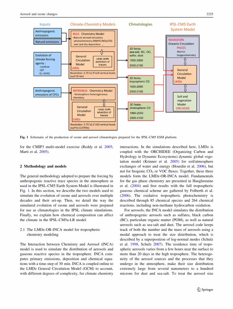
2 Methodology and models

The general methodology adopted to prepare the forcing by

anthropogenic reactive trace species in the atmosphere as

used in the IPSL-CM5 Earth System Model is illustrated in

Fig. 1. In this section, we describe the two models used to

simulate the evolution of ozone and aerosols over multiple

decades and their set-up. Then, we detail the way the

simulated evolution of ozone and aerosols were prepared

for use as climatologies in the IPSL climate simulations.

Finally, we explain how chemical composition can affect

the climate in the IPSL-CM5a-LR model.

2.1 The LMDz-OR-INCA model for tropospheric

chemistry modeling

The Interaction between Chemistry and Aerosol (INCA)

model is used to simulate the distribution of aerosols and

gaseous reactive species in the troposphere. INCA com-

putes primary emissions, deposition and chemical equa-

tions with a time-step of 30 min. INCA is coupled online to

the LMDz General Circulation Model (GCM) to account,

with different degrees of complexity, for climate chemistry

interactions. In the simulations described here, LMDz is

coupled with the ORCHIDEE (Organizing Carbon and

Hydrology in Dynamic Ecosystems) dynamic global vege-

tation model (Krinner et al. 2005) for soil/atmosphere

exchanges of water and energy (Hourdin et al. 2006), but

not for biogenic CO2 or VOC fluxes. Together, these three

models form the LMDz-OR-INCA model. Fundamentals

for the gas phase chemistry are presented in Hauglustaine

et al. (2004) and first results with the full tropospheric

gaseous chemical scheme are gathered by Folberth et al.

(2006). The oxidative tropospheric photochemistry is

described through 85 chemical species and 264 chemical

reactions, including non-methane hydrocarbon oxidation.

For aerosols, the INCA model simulates the distribution

of anthropogenic aerosols such as sulfates, black carbon

(BC), particulate organic matter (POM), as well as natural

aerosols such as sea-salt and dust. The aerosol code keeps

track of both the number and the mass of aerosols using a

modal approach to treat the size distribution, which is

described by a superposition of log-normal modes (Schulz

et al. 1998, Schulz 2007). The residence time of tropo-

spheric aerosols varies from a few hours near the surface to

more than 20 days in the high troposphere. The heteroge-

neity of the aerosol sources and the processes that they

undergo in the atmosphere, make their size distribution

extremely large from several nanometers to a hundred

microns for dust and sea-salt. To treat the aerosol size

Fig. 1 Schematic of the production of ozone and aerosol climatologies prepared for the IPSL-CM5 ESM platform

Aerosol and ozone changes 2225

123

diversity, particles are partitioned into 3 size classes: a sub-

micron (diameters \ 1 lm), a micron (diam. between 1

and 10 lm) and a super-micron class ([10 lm diam.). This

treatment using modes is computationally much more

efficient compared to a bin-scheme (Schulz et al. 1998).

Furthermore, to account for the diversity in chemical

composition, hygroscopicity, and mixing state, we distin-

guish between soluble and insoluble modes. In both sub-

micron and micron-size, soluble and insoluble aerosols are

treated separately. Sea-salt, SO4 and methane sulfonic acid

(MSA) are treated as soluble components of the aerosol.

Dust is treated as insoluble, whereas black carbon (BC) and

particulate organic matter (POM) appear both in the solu-

ble or insoluble fractions. The aging of primary insoluble

carbonaceous particles transfers insoluble aerosol number

and mass to soluble with a half-life of 1.1 days (Cooke and

Wilson 1996; Chung and Seinfeld 2002).

The uptake and loss of water from aerosol particles is

generally fast and depends on the chemical composition,

size and surface properties of the aerosol particle. Aerosol

water is responsible for about 50 % of the global aerosol

column loads. This water uptake modifies the aerosol

optical properties. The nondimensional optical depth, s,

can be expressed as a function of the effective radius of the

aerosol:

s ¼ 3 Q M = 4 qre

where Q is the nondimensional extinction coefficient,

computed using Mie theory, M, is the aerosol burden per

unit area (kg m-2), q is the particle density (kg m-3), and

re, the effective radius (m). As relative humidity increases,

this equation must be modified to account for the presence

of water. The density is then recomputed as the mass-

weighted sum of the dry density of the aerosol and the

density of water. The refractive index, hence the extinction,

is also changed to account for water. We use a formulation

first implemented by Chin et al. (2002) to rewrite the

relationship above as a function of the aerosol dry burden

Mdry (in kg m-2):

s ¼ b Mdry

where b, the specific extinction (m2 kg-1), is computed as

follows:

b ¼ 3 Q M = 4 qre Mdry

The optical properties and hygroscopic growth of sea-salt

were taken from Irshad et al. (2009). For sulfates, we fol-

lowed the relationships published for ammonium sulfate by

Martin et al. (2003). In the case of black carbon and

organic carbon we took the same dependence of hygro-

scopic growth on relative humidity as Chin et al. (2002).

The aerosol scheme is thoroughly explained in Schulz

(2007) and Balkanski (2011). The chemistry of ammonia/

nitrate/ammonium containing aerosols was not considered

in this model version.

2.2 LMDz-OR-INCA set-up

The LMDz-OR-INCA simulations consist of two groups: a

simulation covering the historical 1850–2000 period and a

set of simulations covering four future projections of

emissions for the 2000–2100 period. For the simulation

aiming to represent the evolution of tropospheric compo-

sition over the past period, the emissions provided by

Lamarque et al. (2010) for anthropogenic (including ship

and aircraft) and biomass burning emissions are used.

These emission datasets consist of fluxes for each decade

of methane, carbon monoxide, nitrogen oxides and 23 non-

methane hydrocarbons (specific species or family of com-

pounds) for ozone precursors and black carbon, organic

carbon, ammonia and sulfur dioxide for aerosols and aer-

osol precursors. They have a 0.5� 9 0.5� horizontal reso-

lution. For the 4 future projections, the Representative

Concentration Pathways (RCP) emissions are used and can

be found at [http://www.iiasa.ac.at/web-apps/tnt/RcpDb/].

They correspond to emission trajectories compatible with

the evolution of radiative forcing equivalent in 2100 to 8.5,

6.0, 4.6 and 2.6 W m-2. These scenarios are intended to

span a range of climate forcing levels (Moss et al. 2010)

and are not intended to be associated with any socio-eco-

nomic pathway. Hence, many socio-economic pathways

could potentially be associated with a given RCP scenario.

Methodological elements used to build these projections

can be found in Riahi et al. (2007) for RCP8.5; Fujino et al.

(2006) and Hijioka et al. (2008) for RCP6.0; Clarke et al.

(2007), Smith and Wigley (2006) and Thomson et al.

(2011) for RCP4.5 and van Vuuren et al. (2007) for

RCP2.6. An important point to mention regarding past and

future emissions is the considerable effort made to recon-

cile the main regional and global present-day inventories to

have a common starting point in 2000 for all the projec-

tions and historic reconstructions, which was not the case

in previous works, for example in the IPCC-AR4 simulations

(Lamarque et al. 2010). The assessment of the long-term

trends induced by the use of the historical anthropogenic

emission datasets in global chemical models is discussed in

Lamarque et al. (2010) and is not tackled in this paper. The

historical trends of total aerosols contents and global tropo-

spheric ozone compared to those described in Cionni et al.

(2011) and Lamarque et al. (2011) are shown Figures S6 and

S7 of the supplementary material.

In order to use these fluxes in the INCA model, we

reported the individual hydrocarbon fluxes on INCA spe-

cies or surrogate species as described in Folberth et al.

(2006), we spatially interpolated the fluxes to the model

resolution (3.75� 9 1.9�) and we applied a linear


123

http://www.iiasa.ac.at/web-apps/tnt/RcpDb/

interpolation between decades. The methane oxidation is

computed interactively according to the emissions and not

prescribed on concentrations as often made in such exer-

cises (e.g. Stevenson et al. 2006). The evolution of the CH4

concentrations simulated by LMDz-OR-INCA against

those prescribed in the CMIP5 exercise is presented Figure

S5 in the supplementary material. The anthropogenic and

biomass-burning fluxes, compiled by Lamarque et al.

(2010), are added to natural fluxes used in the INCA

model. All natural emissions are kept at their present-day

levels, except lightning NOx. Hence, for organic aerosols,

the secondary organic matter formed from biogenic emis-

sions is equal to that provided by the AeroCom emission

dataset (Dentener et al. 2006b). The lightning NOx emis-

sions are computed interactively during the simulations

depending on the convective clouds, according to Price and

Rind (1992), with a vertical distribution based on Pickering

et al. (1998) as described in Jourdain and Hauglustaine

(2001). The ORCHIDEE vegetation model was used (off-

line) to calculate biogenic surface fluxes of isoprene,

terpenes, acetone and methanol as well as NO soil emis-

sions as described by Lathiere et al. (2006). Natural

emissions of dust and sea salt are computed using the 10 m

wind components from the ECMWF reanalysis for 2006

and, consequently, have seasonal cycles, but no inter-

annual variability. As described in Hauglustaine et al.

(2004), the stratospheric ozone concentrations are relaxed

toward observations at the altitudes having potential tem-

peratures above 380 K. The ozone observations are taken

from the monthly mean 3D climatologies of Li and Shine

(1995), based on ozone soundings and different satellite

data.

The LMDz general circulation model requires sea sur-

face temperature (SST), solar constant and LL-GHG global

mean concentrations as forcings. For historical simulations,

we use the HADiSST for sea surface temperature (Rayner

et al. 2003) and the evolution of LL-GHG concentrations

compiled in the AR4-IPCC report. For future projections,

we use the LL-GHG concentrations distributed by the RCP

database. No RCP projections from Earth System Model

were available at that time. The SST are from previous

IPSL-CM4 simulations having similar climate trajectories

in terms of radiative forcing evolution. Hence, for the

RCP8.5 projection, we use the SST from IPSL-CM4 sim-

ulation for the SRES-A2 scenario. Analogously, we use the

SRES-A1B for RCP6.0, the SRES-B1 for RCP4.5 and the

scenario E1 (van Vuuren et al. 2007) for the RCP2.6

simulation.

Using the model set-up described above, the LMDz-OR-

INCA is run to generate 3D monthly fields of ozone vol-

ume mixing ratio and aerosol loads (for SO4, POM, SS,

DUST and BC) with a 3.75 9 1.9� horizontal resolution

over 19 vertical levels. In these simulations, the

tropospheric composition simulated by INCA does not

influence the climate simulated by LMDz-OR. The simu-

lations were performed using a vector parallel supercom-

puter, NEC SX-9 system. A century-long simulation takes

3 months on four processors.

2.3 LMDz-REPROBUS model and Set-up

The LMDz-REPROBUS model is used to simulate the

stratospheric chemistry and to produce the stratospheric

ozone climatology. The REPROBUS (Reactive Processes

Ruling the Ozone Budget in the Stratosphere) model

(Lefevre et al. 1994, 1998) interactively calculates the

global distribution of trace gases, aerosols and clouds

within the stratosphere. The model has been extensively

described in Jourdain et al. (2008). It includes 55 chemical

species and the related stratospheric gas-phase and heter-

ogeneous chemistry. Absorption cross-sections and kinetics

data are based on the JPL recommendations (Sander et al.

2006). The photolysis rates are calculated off-line with the

Tropospheric and Ultraviolet visible (TUV) radiative

model (Madronich and Flocke 1998). The heterogeneous

chemistry component takes into account the reactions on

sulphuric acid aerosols, and liquid (ternary solution) and

solid (NAT, ice) Polar Stratospheric Clouds (PSCs). The

gravitational sedimentation of PSCs is also simulated.

For the calculation of the stratospheric ozone fields,

REPROBUS was coupled to a version of the LMDz model,

which extended from the ground up to 65 km, on 50 hybrid

sigma-pressure vertical levels, with a resolution varying in

the stratosphere from about 1 km around the tropopause

region to about 3 at 50 km (Lott et al. 2005). The hori-

zontal resolution is 3.75� in longitude and 2.5� in latitude.

The temporal evolution of the Ozone-Depleting Sub-

stances (ODSs) and GHGs mixing ratios were derived from

observations for the 1961–2006 period, and then according

to one ODS scenario and two different GHG scenarios

from the CCMVal project for the 2007–2100 period: REF2

and SCN-B2c (Morgenstern et al. 2010, Eyring et al.

2010b). The evolution of ODSs in REF2 is based on the

scenario A1 from WMO (2007), but slightly modified to

account for the earlier phase out of HCFCs agreed upon at

the 2007 Meeting of the Parties to the Montreal Protocol

(Morgenstern et al. 2010). Regarding GHGs, REF2 follows

the SRES A1B scenario (IPCC 2001) and is close to the

RCP6.0 scenario. The evolution of GHGs in SCN-B2c is

fixed at 1960 levels; in comparison with REF2 results, this

sensitivity scenario is used to diagnose the respective

contributions of ODSs and GHGs to the evolution of

stratospheric ozone. To be consistent with the evolution of

GHGs, sea surface temperature and sea ice concentration

(SST/SIC) in REF2 were prescribed with the AMIP

(Atmospheric Model Intercomparison Project) climatologies


123

for the past (Kanamitsu et al. 2002) and from results from

IPSL-CM4 simulation following the SRES A1B scenario

(IPCC 2007) for the future because no RCP simulations

from a climate model were available yet. The SST/SIC in

SCN-B2c simulation were prescribed with the 1955–1964

average of the values used in REF2.

Since the stratospheric ozone fields from REF2 follow

the RCP6.0 trajectory, the construction of the fields for

the three other scenarios was required to cover the range of

the four RCP projections. Note that the ODS scenario is the

same for all the RCP scenarios. As a consequence, the

stratospheric RCP fields were reconstructed by interpolat-

ing (for RCP2.6 and RCP4.5 scenarios) or extrapolating

(for RCP8.5) linearly from the REF2 and SCN-B2c

stratospheric ozone series using a time-varying weighting

coefficient proportional to the CO2 mixing ratio. This

simple approach is supported by the finding of a nearly

linear dependence of stratospheric ozone changes on the

change in CO2 level over the range of RCP scenarios

(Eyring et al. 2010a).

2.4 Constructions of climatologies for use

in IPSL-CM5

Ozone variations are now considered in the IPSL-CM5

simulations, which was not the case in previous climate

simulation exercises. To account for the temporal evolution

of both stratospheric and tropospheric ozone, the two

model-calculated ozone datasets computed respectively

with the LMDz-REPROBUS and LMDz-OR-INCA models

are combined in order to produce ozone fields to force the

IPSL coupled ocean–atmosphere model. Tropospheric

ozone fields were simulated by LMDz-OR-INCA over the

1850–2000 period and according to the four RCP scenarios

for the 2000–2100 period. Stratospheric fields are based on

the 1960–2100 REF-2 LMDz-REPROBUS simulation,

corresponding to RCP6.0, and on inter/extrapolations

between REF-2 and SCN-B2c simulations to produce the

three other pseudo-RCP simulations. The choice of tropo-

spheric and stratospheric datasets for each period is sum-

marized in Table 1.

Atmospheric measurements and model simulations

constrained by emission inventories indicate that the

increase in ODS (Ozone Depleting Substances, mostly

CFCs) concentrations was very marginal before 1960

(WMO 2011). Therefore, trends in stratospheric ozone are

expected to be negligible before 1960 compared to post-

1960s stratospheric ozone changes. Therefore, prior to

1960, only the temporal variation in tropospheric ozone is

considered and a 1960s smoothed annual cycle is used for

stratospheric ozone. After 1960, both tropospheric and

stratospheric fields are varying. Raw monthly fields of both

INCA and REPROBUS ozone time series are interpolated,

zonally averaged and temporally smoothed using a 11-year

running mean.

For the merging of the tropospheric and stratospheric

model-calculated ozone series, the first step is to determine

the chemical tropopause (defined as the contours of

150 ppbv of ozone) in all the monthly-mean fields. Then,

the INCA ozone fields are slightly stretched or compressed

in the vertical in order to have the INCA tropopause alti-

tude matching the REPROBUS tropopause altitude.

Finally, REPROBUS and INCA fields are merged at the

chemical tropopause region. The thickness of this transition

region is taken to be about 3 km, extending from 2 km

above the tropopause to 1 km below the tropopause. The

two ozone mixing ratio fields are merged within the tran-

sition region using a sinusoidal interpolation between the

upper or lower limit instead of a standard linear interpo-

lation. The resulting merged field contains INCA fields

below the tropopause region and REPROBUS fields above,

together with a relatively smooth transition from one field

to another within the tropopause region.

There is a large diurnal cycle of ozone in the upper

stratosphere and mesosphere. In order to avoid a diurnal

bias in the radiative transfer calculations, notably of the

heating rates, the IPSL coupled ocean–atmosphere climate

model is forced by monthly-mean day-time and night-time

ozone fields in this altitude range whereas it is forced with

monthly-mean 24 h averaged ozone fields in the rest of the

model domain.

Regarding aerosols, only the sulfate induced radiative

forcing was considered in the previous IPSL-CM4 model

(Dufresne et al. 2005). The historical evolution of sulfate

was prescribed according to decadal means computed by

Boucher and Pham (2002) and its future evolution was

based on SRES-A2 projections (Pham et al. 2005). For the

IPSL-CM5 simulations, the radiative impact of dust, sea

salt, black carbon and organic carbon aerosols were

introduced in LMDz as described in Deandreis (2008) and

Balkanski (2011). The INCA fields are then averaged to

obtain an 11-year running mean with a monthly resolution.

2.5 The IPSL-CM5 platform for Earth system

and climate modeling

This section describes the way ozone and aerosols can

influence the climate in the IPSL-CM5 platform. The solar

radiation code in the LMDz GCM consists of an improved

version of the parameterizations of Fouquart and Bonnel

(1980). The shortwave spectrum is divided into two inter-

vals: 0.25–0.68 and 0.68–4.00 lm. The model accounts for

the diurnal cycle of solar radiation and allows fractional

cloudiness to form in a grid box. The reflectivity and

transmissivity of a layer are computed using the delta

Eddington approximation (Joseph et al. 1996) in the case of


123

Ta

ble

1L

MD

z-O

R-I

NC

Aan

dL

MD

z-R

EP

RO

BU

Ssi

mu

lati

on

su

sed

for

con

stru

ctio

no

fo

zon

ecl

imat

olo

gie

s

Ozo

ne

clim

ato

log

yu

sed

in

IPS

L-C

M5

Tro

po

sph

eric

ozo

ne

fro

mL

MD

z-O

R-I

NC

AS

trat

osp

her

ico

zon

efr

om

LM

Dz-

RE

PR

OB

US

Per

iod

Sce

nar

ioR

un

An

thro

po

gen

ic

emis

sio

ns

of

O3

pre

curs

ors

GH

Gan

dS

ST

for

clim

ate

Ru

nA

nth

rop

og

enic

emis

sio

ns

of

ozo

ne

dep

leti

ng

sub

stan

ceG

HG

and

SS

Tfo

rcl

imat

e

18

50

–1

96

0H

isto

rica

lH

isto

rica

lD

eriv

edfr

om

ob

sD

eriv

edfr

om

Ref

-1(a

ver

age

ov

erth

efi

rst

yea

rs,

rep

rese

nta

tiv

eo

fa

19

60

sst

rato

sph

eric

ozo

ne

con

ten

t)

19

60

–2

00

0R

ef-1

Der

ived

fro

mo

bs

Der

ived

fro

mo

bs

20

00

–2

00

6R

CP

2.6

RC

P2

.6R

CP

2.6

GH

G=

RC

P2

.6

SS

T=

E1

RC

P4

.5R

CP

4.5

RC

P4

.5G

HG

=R

CP

4.5

SS

T=

SR

ES

-B1

RC

P6

.0R

CP

6.0

RC

P6

.0G

HG

=R

CP

6.0

SS

T=

SR

ES

-A1

B

RC

P8

.5R

CP

8.5

RC

P8

.5G

HG

=R

CP

8.5

SS

T=

SR

ES

-A2

20

07

–2

10

0R

CP

2.6

RC

P2

.6R

CP

2.6

GH

G=

RC

P2

.6

SS

T=

E1

Lin

ear

Inte

rpo

lati

on

fro

mR

EF

2an

dS

CN

-B2

C

RC

P4

.5R

CP

4.5

RC

P4

.5G

HG

=R

CP

4.5

SS

T=

SR

ES

-B

1

Lin

ear

Inte

rpo

lati

on

fro

mR

EF

2an

dS

CN

-B2

C

RC

P6

.0R

CP

6.0

RC

P6

.0G

HG

=R

CP

6.0

SS

T=

SR

ES

-A1

B

Ref

-2S

RE

S-A

1?

20

07

Mo

ntr

eal

Pro

toco

lS

RE

S-A

1B

RC

P8

.5R

CP

8.5

RC

P8

.5G

HG

=R

CP

8.5

SS

T=

SR

ES

-A2

Ex

trap

ola

tio

nli

nea

rly

fro

mR

EF

2an

dS

CN

-B2

C

SC

N-B

2c

20

07

–2

10

0

SR

ES

-A1

?2

00

7M

on

trea

lP

roto

col

Der

ived

fro

m1

95

5–

19

64


123

a maximum random overlap (Morcrette and Fouquart

1986) by averaging the clear and cloudy sky fluxes

weighted linearly by their respective fractions in the layer.

The radiative fluxes are computed every 2 h, at the top-of-

atmosphere and at the surface, with and without the pres-

ence of clouds, and with and without the presence of

aerosols. The clear-sky and all-sky radiative effect of aer-

osol components or greenhouse gases is finally obtained by

subtracting from the radiative fluxes the radiative effect of

the respective in 1850 components. For ozone, the aver-

aged day-night ozone is used for longwave whereas only

daylight ozone is used for shortwave computations.

Regarding aerosols, we treat the indirect effect of aerosols

by computing the first indirect effect only. For this effect,

the cloud droplet number is increased with aerosol con-

centrations for constant liquid water content. We do not

consider the second indirect effect that affects the lifetime

of clouds. The number of cloud droplets is calculated

through the prognostic equation from Boucher and Loh-

mann (1995), with the coefficients that were derived from

the Polder satellite measurements by Quaas and Boucher

(2005). The cloud droplet number concentration (CDNC, in

droplets per cm3), is computed from the mass of soluble

aerosol msoluble = mSO4 ? mBC, soluble ? mPOM, soluble,

through the relationship:

CDNC ¼ 101:7þ 0:2 logðmsolubleÞ

considering the parameters described in Dufresne et al.

(2005) and mass (m) in lg m-3.

3 Present-day distribution of aerosols and ozone

In this section we discuss briefly the realism of the present

day distribution of the reactive climate forcing agents.

Since the simulations are performed with a GCM climate

(as opposed to using a CTM or a nudged climate), the

comparison of model results with observations is only

meaningful when considering observations sufficiently

averaged in time to have a climatological representativity.

It would not make sense to attempt to collocate model

results and observations as is done for a full model

evaluation. Moreover, the evaluation of the successive

versions of LMDz-INCA (used in nudged mode) and

LMDz-REPROBUS, particularly in the framework of

international modeling exercises (see references in Sect.

1), gives us confidence in their capabilities to reproduce

ozone and aerosol distributions and their evolution.

However, as with the other global chemical-climate

models (Shindell et al. 2003; Lamarque et al. 2011 and

references therein), LMDz-OR-INCA failed to reproduce

the B10 ppb values of ozone measured in the late nine-

teenth century.

3.1 Tropospheric composition

The LMDz-INCA model results have been extensively

evaluated with surface, aircraft, and satellite observations

of tropospheric oxidants, aerosols, and related species and

the conformity of the results of this GCM version com-

pared with the CTM results has been checked (not shown).

Regarding tropospheric ozone, the LMDz-INCA chemical

results were compared with many other global CTMs or

GCMs, and with observations as part of the international

HTAP (Hemispheric Transport of Air Pollution) and

ACCENT/PhotoComp (Atmospheric Composition Change:

the European NeTwork of excellence) exercises. The

related papers show a response (in terms of sensitivity to

emissions) of LMDz-INCA which is quite similar to the

ensemble mean of the results for ozone (Stevenson et al.

2006). Comparisons with ozone surface network (Ellingsen

et al. 2008) show a systematic positive bias for all the

models, partly due to misrepresentation of NOx gradients

close to the sources. Reidmiller et al. (2009) and Fiore et al.

(2009) tried to discriminate the climatologic features of

ozone measured by the CASTNET (Clean Air Status and

Trends Network; USA) and EMEP (European Monitoring

and Evaluation Programme) networks before comparing

with global models. LMDz-INCA showed in these studies

a fairly good agreement for ozone with US stations.

Figure 2 shows the monthly zonal-mean distribution of

tropospheric ozone in the INCA_REPROBUS climatology

(11-year mean around 2007) and for two remote sensing

based datasets: the NASA-TES dataset (averaged over the

2006–2008 period) and the IASI dataset (averaged over the

2008–2010 period). TES (Tropospheric Emissions Spec-

trometer) is an infrared spectrometer flying aboard the

Aura satellite, the third of NASA’s Earth Observing Sys-

tem (EOS) spacecraft, which has orbited Earth since 2004.

This high resolution Fourier transform spectrometer, has

been flying on a *705 km sun-synchronous polar orbit,

with equator crossing time about 13:43 LST. It provides

global ozone measurements, retrieved from the 9.6 lm

ozone absorption band using the 995–1,070 cm-1 spectral

range. The present study makes use of the TES Version 004

nadir ozone profiles (level 2), collected from

https://wist.echo.nasa.gov/. These profiles are reported on a

vertical grid of 67 standard levels (surface ? 66 levels).

The retrievals and error estimation, already described by

Worden et al. (2004), Bowman et al. (2002, 2006) and

Kulawik et al. (2006) are based on the optimal estimation

approach (Rodgers et al. 2000). TES ozone has been

evaluated on a regular basis since the start of the mission in

2004, and compared against ozone-sonde measurements.

For the previous version, Nassar et al. (2008) indicate a

positive bias comprised in the 3–10 ppbv range for the

upper-troposphere and lower-stratosphere. For the most


123

https://wist.echo.nasa.gov/

recent versions, Boxe et al. (2010) indicate, for the high

latitudes, a positive bias from the surface to the upper-

troposphere, and a negative bias from the upper-tropo-

sphere to the lower-stratosphere. The data have been

selected following the criteria of the TES v004 Data

Users’s Guide (http://tes.jpl.nasa.gov/documents/, access:

September 2011) and of quality flags (SpeciesRetrievalQ-

uality flag = 1, Ozone ‘‘C-Curve’’ flag = 1) developed by

the data providers.

The ozone retrievals from the nadir-viewing Infrared

Atmospheric Sounding Instrument (IASI), launched

onboard the polar-orbiting METOP platform in December

2006, are also shown. TES and IASI are both nadir-viewing

Fourier Transform spectrometers, such that both datasets

have similar characteristics. The main differences are: IASI

has better horizontal coverage (twice daily global coverage

while TES has a 10 days revisit time), but TES has better

spectral resolution (0.1 cm-1 for TES and 0.5 cm-1 for

IASI). The latter results in better vertical resolution for

TES, with *4 independent pieces of information in the

vertical, two of which are in the troposphere, compared

to *3 for IASI. This vertical resolution directly depends

on surface temperatures, with more information above

warm surfaces. The IASI retrievals used in this work are

from the FORLI algorithm, which is also based on optimal

estimation. A full description of the retrieval method and

setup is provided in Coheur et al. (2005) and Boynard et al.

(2009). The validation against ozone sondes in the mid and

tropical latitudes performed by Boynard et al. (2009), Keim

et al. (2009) and Dufour et al. (2011) shows good agree-

ment in terms of tropospheric partial columns. They all

note, however, a tendency to overestimate ozone, espe-

cially in the tropopause region. The UTLS bias (12 %) is

partly compensated by a low bias in the lower troposphere

(-7 %). The observed biases in the UTLS are most likely

linked to the instrumental limitations in terms of vertical

sensitivity (large correlations between vertical levels).

Information on the troposphere will be particularly limited

above cold surfaces, so that the performance is expected to

be lower in polar regions (low sensitivity to the lower

troposphere, lower tropopause). Here, a monthly-mean

climatology based on the retrievals in 2008 to 2010 has

been constructed using filters based on retrieval errors

recommended by the retrieval team (D. Hurtmans, personal

communication) to keep only the most accurate data. An

accurate, quantitative, comparison between model and

Pre

ssur

e (m

illib

ar)

Model climatology (2002-2012) TES (2006-2008) IASI (2008-2010)

Zonal Mean Ozone

0 10 20 4030 50 60 70 80 90 100 110ppb

Pre

ssur

e (m

illib

ar)

1000

800

600

400

200

0

1000

800

600

400

200

0

LatitudeLatitude

80°S 40°S 0° 40°N 80°N 80°S 40°S 0° 40°N 80°N 80°S 40°S 0° 40°N 80°N

Latitude

january

july

Fig. 2 Monthly averaged zonal-mean ozone distribution in ppbv. The model results (left column) are averaged over a 11 year period centered

around 2007. The remote sensing based ozone is obtained using the TES dataset averaged over the 2006–2008 period (middle column) and using

the IASI dataset over the 2008–2010 period (right column)


123

http://tes.jpl.nasa.gov/documents/

observations would require that each instrument’s vertical

sensitivity characteristics be taken into account (i.e. the

calculation of model profiles smoothed with the averaging

kernels). Since precise validation was not the purpose here,

only a simple, direct comparison was undertaken.

Comparing with TES data, the ozone mixing ratios are

satisfactorily well reproduced by the climatology with

values of a few tens ppbv at the surface increasing with

altitude and a North/South gradient due to the distribution

of emissions. The northern free tropospheric values are

slightly underestimated by the model with differences of

10–25 ppbv at 500 hPa at northern midlatitudes. Elsewhere

in the troposphere the underestimation is lower than

10 ppbv. An overestimation appears in the upper tropo-

sphere (P \ 400 hPa) at the Southern mid latitudes

(30�S:60�S) but not exceeding 20 ppbv. Such differences

between the model results and the TES data are partly

explained by the TES bias found by Nassar et al. (2008)

and Boxe et al. (2010) and are in the lower range of those

reported for four state-of-the-art global chemistry climate

models in Aghedo et al. (2011). For IASI, direct compar-

ison is trickier due to the coarser vertical resolution, and

would require comparisons of integrated columns. It is

interesting to note, however, that the discrepancies between

TES and the model-based climatology remain lower than

the differences between two similar satellite sensors.

In order to quantify the potential impact of the model/

TES discrepancies on the evaluation of radiative forcing of

ozone, Aghedo et al. (2011) defined the instantaneous

radiative forcing kernels (IRFK). The IRFK represent the

sensitivity of outgoing longwave radiation to the vertical

and spatial distribution of ozone under all-sky conditions.

This sensitivity reaches its maximum in the tropical free

troposphere (between 550 and 300 hPa) with values

reaching 0.6–0.8 mW m-2 ppbv-1. It means that a

10 ppbv systematic underestimation could lead, locally, to

a 0.07 W m-2 underestimation of the radiative forcing

according to Aghedo et al. (2011). In this particularly

sensitive region of the troposphere, the mean difference

between the climatology and TES is -3.2 ppbv

(i.e. *5–10 % of the absolute global value) leading to a

possible underestimation of 0.024 W m-2 of the radiative

forcing.

The aerosol optical depth (AOD) contains contributions

from the different aerosol species. Total AOD is often used

to evaluate aerosol simulations because of the availability

of global observational datasets e.g. from Aeronet. The

split of AOD into contributions from aerosol species is of

interest, for example to attribute radiative forcing to scat-

tering and absorbing aerosols. We first evaluate, for each

aerosol type, the LMDz-OR-INCA results for the year

2000 compared with the AeroCom multi-model ensemble

from phase I (Textor et al. 2006), representing year 2000,

and the range of model results from the AeroCom phase II,

representing the year 2006 (see Fig. 3). Considering that

the emissions are different, the LMDz-OR-INCA results

are close to the AeroCom database (i.e. within 25–75 %

percentile distribution of model results) for black carbon,

dust, sea-salts and total aerosol. The POM optical depth is

slightly higher than the mean. The SO4 content is outside

the 25–75 % percentile interval with a 50 % overestima-

tion of the total content compared with the median value.

Compared with the results from the CAM-CHEM model

using the same emissions (Lamarque et al. 2010), the black

carbon burdens are identical both in 1850 and 2000, the

sulfate burden is 15 % lower in INCA for the 2000 year

and the burden of particulate organic matter is 80 % higher

in INCA but at least 2/3 of this discrepancy arises from the

consideration of secondary organic aerosol from natural

sources in the POM category. Altogether total AOD is

close to the median from current models used for the

AeroCom phase II. For each species, the spatial concor-

dance between these INCA results and the AeroCom

median can be checked Figures S2, S3 and S4 of the

supplementary material. The order of magnitude of the

maxima and their location are captured (keeping in mind

that the years are not the same and that interannual vari-

ability is large for species with natural sources).

We secondly evaluate the AOD fields against observa-

tions. Given we read in the aerosol mass fields from

LMDz-OR-INCA into the IPSL-CM5a-LR, the final AOD

affecting the climate model runs differs slightly because of

humidity fluctuations and synoptic variations (different in

the two model versions). We thus chose to evaluate both

the LMDz-OR-INCA field for year 2000 and the decadal

mean for 2000–2009 from the IPSL-CM5a-LR historical

Fig. 3 Optical Depth of the INCA model (red triangles) for total

aerosol and the aerosol species against the AeroCom phase I model

median (black dots). The spread of recent AeroCom phase II results is

shown as box and whisker plot with minimum, 25 % percentile,

median, 75 % percentile and maximum. Note that total AOD is scaled

by a factor 0.5 and Black Carbon OD by 10


123

base run against a climatological dataset constructed from

Aeronet sun photometer data covering 2000–2009 (Schulz

and Aerocom team 2011). Figure 4 shows the basic sta-

tistics of monthly aggregated data at the Aeronet surface

sites for these two model results. The same statistics are

obtained for representative AeroCom model results, range

and median of the models. The AeroCom ensemble multi-

model mean outperforms most models. The INCA and

IPSL show slightly lower correlation with observed AOD

than the recent AeroCom phase II results. However, these

latter have specifically used 2006 meteorology and emis-

sions representative of the last part of the decade. In terms

of RMS errors, the models are rather similar. At the Aer-

onet sites the mean AOD of the LMDz-OR-INCA model is

close to the median of the recent state-of-the-art multi-

model ensemble. The performance of the IPSL-CM5a-LR

AOD field is slightly better than the LMDz-OR-INCA

forcing model AOD field. This might reflect the fact that

we use the decadal mean of the whole decade from the

IPSL climate model run, and only the year 2000 from

the INCA model run. All in all it shows the realism of the

AOD fields used in the IPSL-CM5 model (see also figure

S1 in the supplementary material).

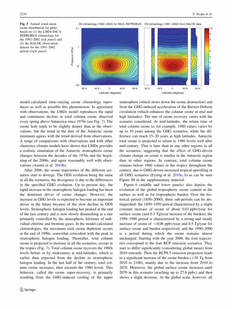
3.2 Stratospheric ozone

The LMDz-REPROBUS model simulations of strato-

spheric ozone used to build the climatologies for the IPSL-

CM5 for the 1850–2006 period have been evaluated

against other chemistry-climate models and a wide range of

observations (Jourdain et al. 2008; Austin et al. 2010a, b;

Gettelman et al. 2009a, b; Hegglin et al. 2010; Morgenstern

et al. 2010). Figure 5 shows a comparison between the

model-calculated and the HALOE (Halogen Occultation

Experiment) observation-based annual zonal mean distri-

butions. The model-calculated distribution reproduces

correctly the maximum of about 10 ppmv near 10 hPa in

the tropics but the model-calculated maximum is a bit

narrower than in the HALOE climatology. In the strato-

sphere, the difference in ozone mixing ratios between the

model-calculated climatology and the HALOE climatology

is generally within 0.5 ppmv, except at high latitudes in the

upper stratosphere due to shortcomings in the transport in

the LMDz-REPROBUS model (Jourdain et al. 2008). In

the mesosphere (above 1 mb level), the ozone mixing ratio

is overestimated compared to HALOE observations which

is not surprising since the model chemistry scheme is only

suited for stratospheric applications.

4 Atmospheric composition change between 1850

and 2100

4.1 Ozone

When analysing total column ozone changes, one has to

keep in mind that about 90 % of the ozone is contained in

the stratosphere. Therefore, total column ozone changes are

generally driven by stratospheric ozone changes. Figure 6

(upper panel) shows the evolution of the model-calculated

globally and annually averaged total column ozone for the

four scenarios since 1960 only. Figure 7 shows the evo-

lution of annually averaged total column ozone as a func-

tion of latitude for the standard scenario RCP6.0. Before

2010, the model-calculated column ozone changes repro-

duce all the major features of the long-term temporal

evolution of column ozone revealed by observations,

mostly satellite, balloon, and ground-based. On a global

scale, the model-calculated total column ozone decreases

by about 4 % from 1960s to the end of the 1990s with most

of the reduction occurring primarily at mid- to high lati-

tudes of both hemispheres. There is no clear trend in the

tropics. All theses features in the model-calculated column

ozone climatology are in line with the trends reported from

observations (WMO 2011; SPARC 2010). In view of the

well-established impact of the so-called ozone hole on the

Antarctic climate (Son et al. 2010), it is important that the

Fig. 4 Statistics of evaluation of aerosol optical depth of the INCA

model and the IPSL-CM5a evaluation against monthly worldwide

Aeronet data climatological mean 2000–2009. Correlation coefficient,

model mean at Aeronet sites (Observations show mean of 0.202) and

RMS error are shown. For comparison, AeroCom phase II model

median is also shown (black dots). The spread of corresponding

recent AeroCom phase II results is shown as box and whisker plot

with minimum, 25 % percentile, median, 75 % percentile and

maximum


123

model-calculated time-varying ozone climatology repro-

duces as well as possible this phenomenon. In agreement

with observations, the LMDz model reproduces the rapid

and continuous decline in total column ozone observed

every spring above Antarctica since 1970s (see Fig. 7). The

ozone hole tends to be slightly deeper than in the obser-

vations, but the trend in the date of the Antarctic ozone

minimum agrees with the trend derived from observations.

A range of comparisons with observations and with other

chemistry-climate models have shown that LMDz provides

a realistic simulation of the Antarctic stratospheric ozone

changes between the decades of the 1970s and the begin-

ning of the 2000s, and agree reasonably well with obser-

vations (Austin et al. 2010b).

After 2006, the ozone trajectories of the different sce-

narios start to diverge. The ODS evolution being the same

in all the scenarios, the divergence is due to the differences

in the specified GHG evolution. Up to present day, the

rapid increase in the stratospheric halogen loading has been

the dominant driver of ozone changes. However, the

increase in GHG levels is expected to become an important

driver in the future because of the slow decline in ODS

levels. Stratospheric halogen loading has peaked at the end

of the last century and is now slowly diminishing at a rate

primarily controlled by the atmospheric lifetimes of indi-

vidual chlorine and bromine gases. In the model-calculated

climatologies, the maximum total ozone depletion occurs

at the end of 1990s, somewhat coincident with the peak in

stratospheric halogen loading. Thereafter, total column

ozone is projected to increase in all the scenarios, except in

the tropics (Fig. 7). Total column ozone recovers the 1960s

levels before or by midcentury at mid-latitudes, which is

earlier than expected from the decline in stratospheric

halogen loading. In the last half of the century, total col-

umn ozone increases, then exceeds the 1960 levels. This

behavior, called the ozone super-recovery, is primarily

resulting from the GHG-induced cooling of the upper

stratosphere (which slows down the ozone destruction) and

from the GHG-induced acceleration of the Brewer-Dobson

circulation (which enhances the column ozone at mid and

high latitudes). The rate of ozone recovery varies with the

scenario considered. At mid-latitudes, the return time of

total column ozone to, for example, 1980 values varies by

up to 10 years among the GHG scenarios, while the dif-

ference can reach 15–20 years at high latitudes. Antarctic

total ozone is projected to return to 1980 levels well after

mid-century. That is later than in any other regions in all

the scenarios, suggesting that the effect of GHG-driven

climate change on ozone is smaller in the Antarctic region

than in other regions. In contrast, total column ozone

remains below 1960 values in the tropics throughout the

century, due to GHG-driven increased tropical upwelling in

all GHG scenarios (Eyring et al. 2010a, b) as can be seen

Figure S8 in the supplementary material.

Figure 6 (middle and lower panels) also depicts the

evolution of the global tropospheric ozone content at the

surface as well as for tropospheric burden. Over the his-

torical period (1850–2000), three sub-periods can be dis-

tinguished: the 1850–1950 period characterized by a slight

constant increase of ozone of about 0.03 ppbv/year for

surface ozone (and 0.3 Tg/year increase of the burden), the

1950–1990 period is characterized by a strong and steady

increase of ozone of *0.06 ppbv/year and 0.5 Tg/year for

surface ozone and burden respectively and the 1990–2000

is a period during which the ozone remains almost

unchanged. Starting with the year 2000, the four trajecto-

ries correspond to the four RCP emission scenarios. They

start to differ significantly (considering global mean) from

2010 onwards. Then the RCP8.5 emission projection leads

to a significant increase of the ozone burden (?30 Tg from

2010 to 2100), mainly due to the increase from 2010 to

2070. Moreover, the global surface ozone increases until

2070 in this scenario (reaching up to 27.6 ppbv) and then

shows a slight decrease. At the global scale, however, all

Latitude (degrees)

Pre

ssur

e (h

Pa)

O3 climatology (1992−2002) for INCA−REPROBUS

80 S 40 S 0 40 N 80 N

0.1

1

10

100

Latitude (degrees)

O3 climatology (1991−2002) from HALOE data

80 S 40 S 0 40 N 80 N

1

2

3

4

5

6

7

8

9

10

Fig. 5 Annual zonal-mean

ozone distribution (in ppm)

based on (1) the LMDz-INCA-

REPROBUS climatology for

the 1992–2002 (left panel) and

(2) the HALOE observation

dataset for the 1991–2002

period (right panel)


123

the precursor emissions from this scenario decrease

strongly after 2030, with the exception of methane. The

global tropospheric ozone increase is mainly due to CH4

and regional precursor emission increases over India and

some parts of Africa (Central and South Africa as well as

Gulf of Guinea). Figure 8 shows the map of surface ozone

differences for each RCP scenario in the 2050s compared

to the present-day. For RCP8.5 (upper left), a significant

decrease of surface ozone in North America is simulated

together with a strong increase over India ([8 ppbv

locally). African surface ozone also exhibits a large

increase (4–8 ppbv) over a large part of the continent and

particularly over the tropics. The responses of Europe and

South America are spatially contrasted and range in 2050

between [0; 4.5] ppbv and [- 1.5; 3.5] ppbv respectively.

The three other scenarios (RCP6.0, 4.5 and 2.6) lead to an

ozone decrease either following a stabilization period (e.g.

between 2010 and 2040 for RCP4.5) or as early as 2010.

Looking at the global scale (Fig. 6), the RCP4.5 and

RCP6.0 trajectories are relatively close. However the

ozone evolution corresponds to relatively different regional

patterns. As shown in Fig. 8, not only the amplitude of

regional changes is different (e.g. a stronger decrease over

USA in RCP4.5 compared with RCP6.0) but also the socio-

Fig. 6 Evolution of ozone between 1850 and 2100 shown as total ozone in the temporally averaged climatology (in DU, upper panel),tropospheric ozone burden in the INCA simulation (in Tg, middle panel) and surface ozone in the INCA simulation (in ppbv, lower panel)


123

economical hypotheses underlying the emission projection

as is the case for Asia. The RCP6.0 leads to an increase of

surface ozone over China and Indonesia whereas RCP4.5

results in a significant decrease over China/Indonesia but in

a strong increase over India. In 2100, while RCP6.0 global

surface ozone decrease is greater than the one of RCP4.5,

the global ozone burden remains close to each other.

The RCP2.6 shows a strong and almost constant ozone

decrease of about 0.07 ppbv/year. The surface ozone

decreases in the northern hemisphere but increases in some

tropical regions. However in this scenario it is surprising to

see that global surface ozone is lower than the 1950s level

from 2070 until the end of the century.

In 2030, the surface ozone trajectories of the four RCPs

lie in the range of previous projections performed with

LMDz-INCA during the PHOTOCOMP project (Szopa

et al. 2006). The RCP projections are comprised between

the scenarios corresponding to the storyboards ‘Maximum

Feasible Reduction’ (matching the RCP2.6) and ‘Current

Legislation’ (matching the RCP8.5) (Dentener et al. 2005).

4.2 Aerosols

Figure 9 shows the evolution of the global aerosol optical

depth at 550 nm between 1850 and 2100 as simulated by

year

Latit

ude

(deg

rees

)Total global mean model−calculated ozone column (D.U.) for run RCP6.0

1960 1980 2000 2020 2040 2060 2080

80

60

40

20

0

−20

−40

−60

−80 220

240

260

280

300

320

340

360

380

400

420

Fig. 7 Evolution of the latitudinal mean total ozone (in Dobson Unit)

during the 1960–2000 historical period and during the 2000–2100

according to the RCP6.0 scenario

Fig. 8 Distribution of surface ozone changes in 2050 compared with 2000 for the 4 RCP scenarios (using 10 year means)


123

LMDz-OR-INCA and averaged using a 11-year running

mean. At the global scale, the historical period can be

divided into three sub-periods: 1850–1950, 1950–1990 and

post 1990 periods. The 1850–1950 period shows a slight,

but constant increase in the aerosol content, mainly due to

the increase of sulfate and black carbon over North-Eastern

America and Europe (with regional changes exceeding a

factor of 10 for sulfates). The 1950–1990 period exhibiting

a strong increase of the global aerosol content slightly

smoothed over, from the 1980s, by the slowdown in sulfate

increase. In the last decade of the twentieth century, the

global content of aerosol is almost stable due to compen-

sation between the strong decrease of aerosols over Europe

and North of America (especially sulfates) and an increase

of all types of aerosols over Southern and Eastern Asia. In

the twenty-first century simulations, an increase with a

growth rate equivalent to that of the 1950–1990 period is

simulated for the first decade of the twenty-first century. It

is explained by a strong increase of particulate organic

matter over central Africa and sulfates over Asia for the

four RCPs. After 2010, the projections show different

evolutions both in term of types of aerosols and regional

Fig. 9 Evolution of the global

aerosol optical depth at 550 nm

between 1850 and 2100 shown

by types of aerosols simulated

by the LMDz-OR-INCA model

and then averaged using a

11-year running mean. The

evolution after 2000 is

simulated according to the

4 RCP scenarios


123

features. The common characteristic is the general decline

in the global aerosol content (and for all anthropogenic

components) between 2010 and 2100. However, two

exceptions to this general decline occur. First, a burst of

sulfates over Asia between 2030 and 2080 in the RCP6.0

scenario leads to a subsequent slowdown of the global total

aerosol decrease. The second notable feature is a delay

(compared to other RCP) of the inversion of the growth

rate in the RCP2.6 scenario due to a large increase of black

carbon content over Asia which precedes a faster decline of

aerosol content finally reaching in 2100 a level close to the

one simulated before 1950 (also for the RCP4.5). The final

content in 2100 for RCP6.0 and 8.5 is equivalent to the

1960s level. Whereas wind fields used to generate dust and

sea-salt uplifts remain the same throughout the entire

simulations, as described above, the dust and sea-salt

contents evolve with time. The large increase of dust AOD

([10 %) is correlated in these simulations with a longer

lifetime, due to a changed pattern of wet deposition in

future climate. Indeed, even if the global value of precip-

itation increases in a warmer climate, the precipitation

changes vary in amplitude and sign depending on the

location (Dufresne et al. this issue). Regarding dust, the wet

deposition is strongly weakened around 40�N due, in par-

ticular, to the precipitation decrease over a large area

around the Black Sea.

In the previous CMIP exercise, the IPSL-CM4 con-

sidered only sulfate evolutions computed by Boucher and

Pham (2002) for historical period and Pham et al. (2005)

for future projections based on the SRES scenarios. For

the historical period, the values and distribution of emis-

sions provided by Lamarque et al. (2010) are similar to

those of Boucher and Pham (2002). The slight decline of

global emissions between 1980 and 1990 is similar. The

Lamarque et al. (2010) dataset extends longer (up to the

year 2000), with a strong emission decline ([16 %) over

the last decade. Some very large differences can be

pointed out between the RCP trajectories and the SRES

scenarios for future projections. In the SRES trajectories,

four of the six scenarios lead to a peak in sulfate content

followed by a rapid decrease, which slowed down around

2080. The two other scenarios exhibited an almost con-

stant value of sulfate load throughout the whole twenty-

first century or a constant decrease leading, at the end of

the century, to a value equivalent to 37 % of the 2000

global content. This last SRES scenario (A1T) is inter-

mediate between the RCP2.6 and RCP4.5 projections

regarding sulfate evolution. However, this scenario was

skewed towards non-fossil energy source. Besides this

drastic scenario, the cleanest realistic scenarios are the B1

family relying on the introduction of clean and resource

efficient technologies together with reductions in material

intensity. Such clean scenarios exhibit higher sulfate

content than the RCP simulations, either temporarily or

over the whole century.

5 Radiative Forcings due to chemical climate forcing

agents

The impact of the evolution in the chemical atmospheric

composition on climate is presented here in terms of

radiative forcing (RF), which represents the radiative

imbalance in the climate system at the top of atmosphere

caused by the addition of a greenhouse gas (or other

change), as stated by the 1st IPCC report (IPCC 1990).

Figure 10 shows the present day radiative forcing for each

anthropogenic chemical forcing agent, both long- and

short-lived, as estimated by the IPSL-CM5a-LR Earth

System Model. Some of them are computed individually

and were archived during the ESM simulations, some

others were computed afterwards with the GCM radiation

scheme to isolate the role of each compound and, as a

consequence, with a slightly different protocol. The total

aerosol direct and indirect effects were diagnosed on-line

and archived during the IPSL-CM5a-LR simulations. For

separate components of the aerosols, radiative forcing

diagnostics are calculated as total instantaneous forcing

referenced to preindustrial aerosols. The present-day cli-

mate is used for these computations whatever the period

investigated. For ozone and LL-GHG, however, they are

referenced to the 1850s GHG content. The RF of gaseous

species are computed considering a 1850s climatological

climate and after thermal adjustment of the stratosphere.

As described in the IPCC (2001) report, the radiative

forcing is defined as the imbalance of the net radiation at

the tropopause since the stratosphere adjusts in a few

months after a perturbation whereas the troposphere adjusts

far more slowly due to the thermal inertia of the oceans. In

order to compute radiative forcing with a thermal adjust-

ment of the stratosphere, the radiative code iterates until

the RF at the top of the stratosphere converges with the RF

at the tropopause. Compared to the evaluation done in the

4th IPCC (2007), which can be considered as a useful

reference point, the respective impacts of the climate

forcing agents are correctly ranked. However, the CO2 and

CH4 RF are respectively under- and overestimated (by at

least 7 and 21 %). The discrepancies between the CO2 RF

computed in this work and the IPCC estimation can be

partly explained by the 10 ppm differences between the

1850 and 1750 levels which are used respectively as ref-

erences. However, for both carbon dioxide and methane

RF, the bias is mainly due to a non up-to-date absorption

spectrum in the radiative code. For other species, in par-

ticular ozone and aerosols, the mean RF computed by

LMDz lies in the 90 % confidence interval of the IPCC


123

report. The first indirect forcing of aerosol (cloud albedo

effect) is estimated at -0.29 W m-2, which is almost equal

to the lowest range of estimation.

During the last decade, the quantification of the first

indirect effect evolved significantly in the successive works

based on the IPSL modeling infrastructure reflecting the

large uncertainties in the mechanisms involved in the

quantification of this effect. Hence, Boucher and Pham

(2002), considering only the sulfate aerosol, computed an

indirect effect of -1 W m-2 between 1850 and 1990 using

the LMDz atmospheric model. Then, efforts were done

to use satellite data to adjust the parameters of the empir-

ical relationship between the cloud droplet number

concentrations and the aerosol mass concentration (see

Sect. 2.5) in the GCM (Quaas and Boucher 2005; Quaas

et al. 2004a, b; Dufresne et al. 2005). These modifications

came in addition to cloud cover changes due to the cou-

pling of the atmospheric model with the ORCHIDEE land

surface model for the hydrological cycle. Still using the

Boucher and Pham (2002) sulfate content, the resulting

indirect forcing was assessed to be -0.2 W m-2 between

1850 and 1995 (Dufresne et al. 2005). More recently,

Deandreis et al. (2011) found a -0.39 W m-2 indirect

forcing for sulfate using the IPSL-ESM reading aerosol

fields computed offline (same configuration as the one

retained in IPSL-CM5) between natural and present-day

aerosol distributions (as simulated for AeroCom and rep-

resenting the year 2000). The reason of the difference with

the value found in this work (-0.29) is twofold. First,

contrary to IPSL-CM4, the mass of all soluble part of

aerosols simulated by INCA (dust, sea-salt, particulate

organic matter and black carbon) is taken into account,

which can lead to an increase of the number of cloud

condensation nuclei, where the sulfate concentrations are

low. It results in an increase of a few tens of milliwatts per

square meters of the global indirect effect (Deandreis,

personal communication) since the relation between

CDNC and aerosol concentration is highly non-linear and

reaches a plateau beyond a 50 lg m-3 aerosol content

(Deandreis et al. 2011, Fig. 1). Secondly, the IPSL-CM5a-

LR configuration leads to a significantly colder climate

than the IPSL-CM4 configuration (-0.7 K on the global

mean temperature), which can lead to an increase of low

level cloud cover (Brient and Bony 2012, this issue). Such

increased cloud cover, if matching the aerosol distribution,

is favourable to an increase of the indirect aerosol effect

(Dufresne et al. 2005). The indirect effect estimation will

Fig. 10 Global averaged radiative forcing (RF) estimates in 2000s in

the IPSL-CM5 model for anthropogenic carbon dioxide (CO2),

methane (CH4), nitrous oxide (N2O), chlorofluorocarbons (CFCs),

and 2000 for tropospheric and stratospheric ozone and aerosols (blackand organic carbon, sulfates). The pastel bars indicate the RF values

reported in the IPCC 2007 with their 90 % confidence interval

Fig. 11 Top of atmosphere shortwave radiative forcing due to three anthropogenic aerosol components in 2000


123

probably increase in the coming version of the IPSL

infrastructure IPSL-CM5b, in which low-mid level cloud

coverage is improved (and increased) thanks to more

sophisticated physical parameterizations, in particular the

convective boundary layer representation (Hourdin et al.,

this issue).

The geographical pattern of the RF for the year 2000 is

presented for different aerosol components (Fig. 11), for

total aerosols (Fig. 12) and tropospheric ozone (Fig. 13).

The regional feature of the influence of aerosols is well

represented with regional maximum cooling due to sulfates

exceeding -3 W m-2 over Europe, East Coast of USA,

Asia and the Arabian sea and a warming reaching up to

2 W m-2 due to black carbon over Asia and over the Gulf

of Guinea. As a consequence, the total direct aerosol

forcing is maximal over central Europe, Arabian Sea, Bay

of Bengal, Red Sea and Yellow Sea where the cooling

exceeds -2 W m-2. Figure 14 (lower panels) illustrates

the contrast in the evolution in term of aerosol RF over

Asia and Europe. The indirect cooling effect occurs mostly

over ocean associated with large areas having the highest

values along the North Western African coast in the North

Atlantic and off the Japan coast in North Pacific.

For tropospheric ozone, the forcing is almost exclusively

positive and shows the highest values between 15�N and

40�N, with maximum values ([0.7 W m-2) over a large

area surrounding the North Africa/Arabian Peninsula and

India, as already found by previous studies (e.g. Gauss

et al. 2006).

Figures 14 and 15 show the evolution of the RF due to

ozone and aerosols respectively throughout the twentieth

and twenty-first centuries. The radiative forcing of tropo-

spheric ozone evolves similarly to the ozone burden. After

a stabilization period around 0.4 W m-2 between 1990 and

2010, RF increases in the RCP8.5 scenario, reaching

0.62 W m-2 in 2100. The RF in RCP6.0 and RCP4.5 starts

to decrease after 2060, reaching 0.3 W m-2 in 2100. The

RCP2.6 leads to a constant decrease of the tropospheric

ozone RF after 2010 leading to 0.16 W m-2 in 2100. This

positive RF is partly counteracted by the negative RF of

stratospheric ozone. For the historical period, the strato-

spheric ozone RF peaks in the 1990s (-0.15 W m-2)

before reaching around 2030–2040 a stabilization period

with a lower impact (*-0.1 W m-2). The stratospheric

ozone RF projections from the different scenarios diverge

after 2040. In RCP8.5 and, to a lesser extent, in RCP6.0,

the stratospheric ozone RF increases (decreases if the sign

is taken into account) again throughout the second part of

the century to reach values well below the maximum RF of

the 1990s. For example, it reaches -0.25 W m-2 in 2090

in the RCP8.5 scenario. In contrast, the stratospheric ozone

RF remains constant in RCP4.5 and even decreases in the

RCP2.6. The differences are due to the differences in the

evolution of ozone in the tropical lower stratosphere.

Indeed, as discussed by Forster (1999), the global strato-

spheric ozone RF is very sensitive to the ozone trend

assumed in the tropical lower stratosphere (Hansen et al.,

2005). For example, he found that including in RF calcu-

lations not statistically significant ozone trends in the

tropical lower stratosphere would modify the results by

several fold. In all the scenarios, tropical lower strato-

spheric ozone decreases throughout the twenty-first cen-

tury. The main mechanism driving this evolution is the

GHG-driven increase in tropical upwelling during the

twenty-first century, which is a robust feature in the CCM

simulations (WMO 2011). The increase in tropical

upwelling is the strongest in RCP8.5, the scenario with the

maximum increase in GHG. As a result, the tropical lower

Fig. 12 Shortwave direct and indirect radiative forcing due to all

type of aerosols in 2000 computed by the IPSL-CM5 ESM model


123

stratospheric ozone decrease is also the most pronounced in

RCP8.5 and hence the negative RF carries on decreasing.

At the other end of the scenario spectrum, in RCP4.0 and

RCP2.6, the increases in the tropical upwelling and in the

associated ozone depletion are much more limited

throughout the twenty-first century, leading to much

smaller changes in the stratospheric ozone RF (WMO

2011). Note that the ozone RF trajectories presented here

match well those presented in Cionni et al. (2011) for the

same scenario even if the absolute values of RF are slightly

higher, but still within the AR4 interval.

Figure 16 shows the response of direct radiative forcing

caused by aerosols as a function of the total AOD. Some

subsets of the simulations show linear relationships

between AOD and RF but the slope can differ strongly

between the subsets. On the contrary, for some part of the

simulations, no evident link between RF and AOD can be

found. In fact, since the geographic pattern of the aerosol

radiative effect is heterogeneous, the sensitivities of the

total aerosol direct RF to the trends in aerosol loads vary

depending on the region and type of aerosols dominating

the aerosol changes. Between 1880 and 1980, the increase

in aerosol is dominated by the increase in sulfate aerosol

and consequently, the direct RF is continuously decreasing

reaching -0.34 W m-2 in 1980. Then, from 1980 to 2000,

the increasing fraction of absorbing aerosols (even if the

global content of total aerosol remains almost constant)

tends to attenuate the general cooling effect of aerosol,

which stabilizes during the first years of the twenty-first

century around -0.3 W m-2. That is not the case for

indirect forcing, which stabilizes as soon as 1980 (around

-0.28 W m-2) and seems not affected by the nature

change of aerosol. Between 1995 and 2006 there is no clear

relationship between RF and loads. After 2006, RCP8.5,

4.5 and 6.0 have decreasing total aerosol trajectories,

leading to a reduction of the direct global cooling of

aerosol. The absolute value of RF decreases linearly with

loads but with different slope pointing out the different

underlying hypothesis used for each scenario. Figure 17

presents the spatial distribution of the direct radiative

forcing of aerosols in 2050 and 2100 for the four RCP

scenarios. It clearly confirms how different the regional

evolution can be among the scenario as well as the regional

intensity of the forcing especially over Asia. Hence, the

RCP6.0 scenario induces a strong cooling effect over Asia

(with values exceeding -5 W m-2 over East China) in the

middle of the twenty-first century. Even if the RCP6.0

trajectory is very different over Asia, it does not perturb the

continuous attenuation of the indirect effect at the global

scale, but it leads to a significant peak of the global cooling

effect resulting from direct forcing. In 2100, the effects are

weaker than -2 W m-2 everywhere and for all scenarios,

which is less than the present effect of sulfates alone.

Figure 18 presents the evolution of the RF over the

1850–2100 period considering the RCP8.5 projection for

all the atmospheric climate forcing agents considered in the

IPSL-CM5 model. According to the RCP projections, the

cooling effect of aerosol becomes small in the twenty-first

Fig. 13 Top of atmosphere

radiative forcing due to

tropospheric ozone in 2000


123

century compared to the GHG increase. This is true for all

RCP scenarios as can be seen in Dufresne et al. (this issue).

This was already pointed out by Dufresne et al. (2005) for

SRES projections but it is even more striking here because

of (1) RCP projections relying on a strong emission

decrease for aerosols, (2) black carbon, having a warming

effect, which was added to the atmospheric model and (3)

indirect effect, weaker than in first estimates within the

IPSL modeling infrastructure. The ozone is also now

considered in these simulations and plays a warming role

during the whole twenty-first century (considering total

ozone) according to these scenarios. The amplitude of the

total ozone effect is of the same order as that of the cooling

effect of aerosol.

Among the perspectives to improve the quantification of

chemical compounds on the climate system, the on-line

simulations of atmospheric composition are a promising

way. Hence, Deandreis et al. (2011), show an impact

equivalent of 30 % of the direct radiative forcing solely

due to the impact of a high frequency variation of sulfates

(compared with monthly mean) on radiative forcing

computations. Furthermore, although computationally

costly, only on-line chemistry-climate simulations would

allow quantification of regional feedbacks such as ozone

impact on vegetation or via interplay between carbon and

nitrogen biogeochemical cycles both being directly or

indirectly linked to VOC/NOx/OH gaseous chemistry,

secondary organic aerosols and ammonia/nitrate equilib-

rium. According to RCP projections, the ammonia emis-

sions increase in all the RCP scenarios during the twenty-

first century with 2100 values corresponding to a 50 %

increase of the 2000 emissions. According to the recent

Bellouin et al. (2011) study, nitrate aerosols could partially

replace sulfate aerosols in the climate system in the

remainder twenty-first century. The combining of tropo-

spheric and stratospheric ozone fields is also a weakness of

this work and a single model including both chemical

schemes would allow more consistency for the upper tro-

posphere-lower stratosphere ozone distribution and strato-

sphere/troposphere exchanges.

As always in such projection exercise, the emissions can

not cover all possible futures. Smith et al. (2011) warn

Fig. 14 Evolution of the direct and indirect radiative forcings of aerosol at the global scale and of the direct forcings over Asia and Europe


123

Fig. 15 Evolution of the tropospheric and stratospheric ozone radiative forcings for historical period and RCP scenarios

Fig. 16 Direct radiative forcing as a function of total aerosol depth. The linear trend as well as corresponding correlation coefficients are

specified


123

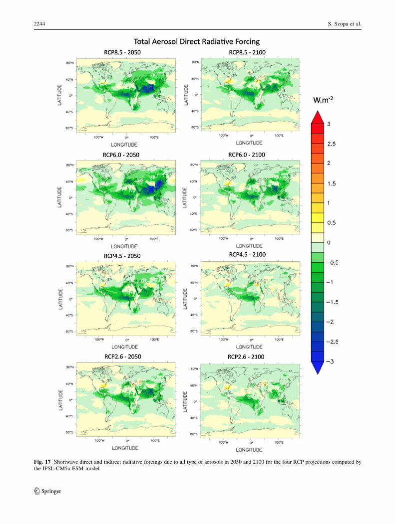
Fig. 17 Shortwave direct and indirect radiative forcings due to all type of aerosols in 2050 and 2100 for the four RCP projections computed by

the IPSL-CM5a ESM model


123

against the air pollutant hypothesis underlying the RCP

scenarios arguing that they are not necessarily consistent

with arbitrary socio-economic pathways. Indeed, these

scenarios have in general allowed emission controls to

increase with income. Nevertheless, the link between

income and pollutant emissions is far more complex with

non-linear relationships between emissions and regional

concentrations as well as air pollution transport from one

region to another. Furthermore, the cost of emission

reductions will differ due to geographical specificities,

emissions density or population levels (Smith et al. 2011).

6 Conclusion

Simulations of the global aerosol (dust, sea-salt, black

carbon, particulate organic matter and sulfates) and ozone

(tropospheric and stratospheric) distributions between 1850

and 2100 have been performed following a recent historical

emission dataset and under the Representative Concentra-

tion Pathways (RCP) for the future. In these simulations,

only biomass burning and anthropogenic sources are vary-

ing from year-to-year. The RCP projections, defined in the

IPCC-AR5 framework, allow to investigate four emission

trajectories for the 2000–2100 period. Each emission tra-

jectory is compatible with a distinct climate pathway and

includes gridded emissions for aerosol and ozone precursors

in decadal increment. These simulations were subsequently

used by the two French Earth System Models (ESMs) to

account for the spatial and temporal evolution of both

radiatively and chemically active compounds, when simu-

lating the climate evolution. This paper presents the meth-

odology used to prepare such climatologies for ESMs. Main

characteristics and trends shown by the climatologies are

discussed for both ozone and aerosols.

The model-calculated present-day distribution of tro-

pospheric ozone is qualitatively compared with two space-

borne thermal infrared spectrometers. Overall, the zonal

distribution appears to be correctly reproduced in the

model-calculated climatology including the summer

increase of ozone in the lower levels of Northern mid-

latitudes. The discrepancies between the model results and

satellite datasets are rather small compared with the dif-

ferences between the two remote sensor-based datasets.

The present-day global mean optical depth for each type of

aerosol is compared with a large multi-model database.

The model results are found to be consistent with the multi-

model dataset for total aerosol, even if the sulfate content is

slightly higher than the multi-model median. The model-

calculated stratospheric ozone distribution is also found to

reproduce most of the features of a well-established satel-

lite-based climatology.

The past negative stratospheric ozone trends, most

apparent in the CFC-induced decline in polar ozone

Fig. 18 Evolution of the individual radiative forcings due to chemical climate forcing agents as considered in the IPSL-CM5 historical and

RCP85 simulation


123

decrease between the 1970s and 1990s, is properly repro-

duced and results in a negative climate forcing culminating

at -0.15 W m-2 in the 1990s. In the meantime, the tro-

pospheric ozone burden increases due to rising fossil-fuel

consumption and generates a positive climate forcing

peaking at 0.41 W m-2, according to our model compu-

tations. The future evolution of ozone strongly depends on

the RCP scenario considered. In RCP4.5 and RCP6.0, the

evolutions of both stratospheric and tropospheric ozone

generate relatively weak radiative forcing changes until

2060–2070 followed by a 30 % decrease in radiative

forcing (in relative values) by 2100. In contrast, RCP8.5

and RCP2.6 model projections exhibit strongly different

ozone radiative forcing trajectories. In the RCP2.6 sce-

nario, both effects (stratospheric ozone, a negative forcing,

and tropospheric ozone, a positive forcing) decline towards

1950s values while they both get stronger in the RCP8.5

scenario. Whereas the tropospheric ozone radiative forcing

is correlated to the tropospheric ozone burden increase in

the past and the future, the evolution of the stratospheric

ozone forcing may be more correlated with the evolution of

ozone content in the tropical lower stratosphere than with

the stratospheric ozone burden.

Over the twentieth century, the evolution of the total

aerosol burden is characterized (according to the emission

dataset available) by a strong increase after World War II

until the middle of the 1980s followed by a stabilization

during the last decade due to the strong decrease in sulfates

in OECD countries since the 1970s. According to the RCP

scenarios, after peaking around 2010, the aerosol content is

projected to decline strongly during the twenty-first century

either monotonically for RCP8.5, 4.5 and 2.6 or after

peaking around 2050 for the RCP6.0 scenario. This com-

mon feature in the emission scenario is strongly different

from the SRES trajectories used for the previous IPCC

report. As a consequence the relative importance of the

total cooling effect of aerosols becomes weaker throughout

the twenty-first century compared with the positive forcing

of GHG. This is due in particular to the inclusion of black

carbon positive forcing during the first half of the century

followed by the emission decline during the second half of

the century.

Nevertheless, both surface ozone and aerosol contents

show very different regional features depending on the

future scenario considered. These regional differences are

of crucial interest regarding the impact of surface ozone on

vegetation or on air quality index and regarding regional

aerosol-driven climate feedbacks.

Acknowledgments Computer time was provided by the CCRT/

GENCI computer center of the CEA. This research was supported by

CNRS, via the INSU-LEFE French Program under the project MIS-

TERRE and by the PRIMEQUAL project called Salut’air. The IPSL-

CM5 model development and the IPSL-CM5 simulations were

performed by the ‘‘IPSL Climate Modeling Center’’. The authors are

thankful for their technical help in carrying the INCA simulations out.

The authors are grateful to the LATMOS (J. Hadji-Lazaro,

M. George, C. Clerbaux) and the ULB (P.F. Coheur, D. Hurtmans)

IASI teams for the availability of the IASI ozone retrievals and their

support in the data analysis. They also acknowledge the Ether French

atmospheric database (http://ether.ipsl.jussieu.fr) for providing the

IASI data and CNES for financial support. The TES data were

obtained from the NASA Langley Research Center Atmospheric

Science Data Center. The authors acknowledge the TES-NASA team

for the availability of ozone level 2 retrievals and the TES Pis

(A. Eldering, J. Worden, R. Beer) from the Jet Propulsion Laboratory,

NASA.

Open Access This article is distributed under the terms of the

Creative Commons Attribution License which permits any use, dis-

tribution, and reproduction in any medium, provided the original

author(s) and the source are credited.

References

Aghedo AM, Bowman KW, Worden HM, Kulawik SS, Shindell DT,

Lamarque JF, Faluvegi G, Parrington M, Jones DBA, Rast S

(2011) The vertical distribution of ozone instantaneous radiative

forcing from satellite and chemistry climate models. J Geophys

Res 116:D01305. doi:10.1029/2010JD014243

Austin J et al (2010a) The decline and recovery of total column ozone

using a multi-model time series analysis. J Geophys Res 115:

D00M10. doi:10.1029/2010JD013857

Austin J et al (2010b) Chemistry-climate model simulations of spring

Antarctic ozone. J Geophys Res 115:D00M11. doi:10.1029/2009

JD013577

Balkanski Y (2011) L’Influence des Aerosols sur le Climat—These

d’Habilitation a Diriger des Recherches. Universite Versailles

Saint Quentin, France

Bellouin N, Rae J, Jones A, Johnson C, Haywood J, Boucher O (2011)

Aerosol forcing in the Climate Model Intercomparison Project

(CMIP5) simulations by HadGEM2-ES and the role of ammo-

nium nitrate. J Geophys Res 116:D20206. doi:10.1029/2011

JD016074

Boucher O, Lohmann U (1995) The sulfate –CCN– cloud albedo

effect—a sensitivity study with two general circulation models.

Tellus Ser B 47:281–300

Boucher O, Pham M (2002) History of sulfate aerosol radiative

forcing. Geophys Res Lett 29(9). doi:10.1029/2001GL0140148

Bowman KW, Steck T, Worden HM, Worden J, Clough S, Rodgers C

(2002) Capturing time and vertical variability of tropospheric

ozone: a study using TES nadir retrievals. J Geophys Res

107(D23):4723. doi:10.1029/2002JD002150

Bowman KWEt et al (2006) Tropospheric emission spectrometer:

retrieval method and error analysis. IEEE Trans Geosci Remote

Sens 44(5):1297–1307. doi:10.1109/TGRS.2006.871234

Boxe CS, Worden JR, Bowman KW, Kulawik SS, Neu JL, Ford WC,

Osterman GB, Herman RL, Eldering A, Tarasick DW, Thomp-

son AM, Doughty DC, Hoffmann MR, Oltmans SJ (2010)

Validation of northern latitude tropospheric emission spectrom-

eter stare ozone profiles with ARC-IONS sondes during ARC-

TAS: sensitivity, bias and error analysis. Atmos Chem Phys

10I(20):9901–9914. doi:10.5194/acp-10-9901-2010

Boynard A, Clerbaux C, Coheur P-F, Hurtmans D, Turquety S,

George M, Hadji-Lazaro J, Keim C, Meyer-Arnek J (2009)

Measurements of total and tropospheric ozone from IASI:


123

http://ether.ipsl.jussieu.fr

http://dx.doi.org/10.1029/2010JD014243

http://dx.doi.org/10.1029/2010JD013857

http://dx.doi.org/10.1029/2009JD013577

http://dx.doi.org/10.1029/2009JD013577

http://dx.doi.org/10.1029/2011JD016074

http://dx.doi.org/10.1029/2011JD016074

http://dx.doi.org/10.1029/2001GL0140148

http://dx.doi.org/10.1029/2002JD002150

http://dx.doi.org/10.1109/TGRS.2006.871234

http://dx.doi.org/10.5194/acp-10-9901-2010

comparison with correlative satellite, ground-based and ozone-

sonde observations. Atmos Chem Phys 9:6255–6271. doi:

10.5194/acp-9-6255-2009

Brient F, Bony S (2012) Interpretation of the positive low-cloud

feedback predicted by a climate model under global warming.

Clim Dyn. doi:10.1007/s00382-011-1279-7

Chin M, Ginoux P, Kinne S, Holben BN, Duncan BN, Martin RV,

Logan JA, Higurashi A, Nakajima T (2002) Tropospheric

aerosol optical thickness from the GOCART model and com-

parisons with satellite and sun photometer measurements.

J Atmos Sci 59:461–483

Chung SH, Seinfeld JH (2002) Global distribution and climate forcing

of carbonaceous aerosols. J Geophys Res 107. doi:10.1029/

2001JD00397

Cionni I, Eyring V, Lamarque JF, Randel WJ, Stevenson DS, Wu F,

Bodeker GE, Shepherd TG, Shindell DT, Waugh DW (2011)

Ozone database in support of CMIP5 simulations: results and

corresponding radiative forcing. Atmos Chem Phys 11:11267–

11292. doi:10.5194/acp-11-11267-2011

Clarke L, Edmonds J, Jacoby H, Pitcher H, Reilly J, Richels R (2007)

Scenarios of greenhouse gas emissions and atmospheric con-

centrations. Sub-report 2.1A of synthesis and assessment product

2.1 by the US climate change science program and the

subcommittee on global change research. Department of Energy,

Office of Biological and Environmental Research, Washington,

DC, USA, vol 7, 154 pp

Coheur P-F, Barret B, Turquety S, Hurtmans D, Hadji-Lazaro J,

Clerbaux C (2005) Retrieval and characterization of ozone

vertical profiles from the IMG nadir high-resolution thermal

infrared remote sounder. J Geophys Res 110:D24303. doi:

10.1029/2005JD005845

Cooke WF, Wilson JJN (1996) A global black carbon aerosol model.

J Geophys Res 101:19395–19409

Deandreis C (2008) Impact des aerosols anthropiques sur le climat

present et future, These de Doctorat de l’Universite Pierre et

Marie Curie, Paris VI

Deandreis C, Balkanski Y, Dufresne JL, Cozic A (2011) Radiative

forcing estimates in coupled climate-chemistry models with

emphasis on the role of the temporal variability. Atmos Chem

Phys Discuss 11:24313–24364. doi:10.5194/acpd-11-24313-

2011

Dentener F, Stevenson D, Cofala J, Mechler R, Amann M,

Bergamaschi P, Raes F, Derwent R (2005) The impact of air

pollutant and methane emission controls on tropospheric ozone

and radiative forcing: CTM calculations for the period

1990–2030. Atmos Chem Phys 5:1731–1755. doi:10.5194/acp-

5-1731-2005

Dentener F et al (2006a) Global atmospheric environment for the next

generation. Environ Sci Technol 40:3586–3594

Dentener F, Kinne S, Bond T, Boucher O, Cofala J, Generoso S,

Ginoux P, Gong S, Hoelzemann J, Ito A, Marelli L, Penner J,

Putaud J-P, Textor C, Schulz M, van der Werf G, Wilson J

(2006b) Emissions of primary aerosol and precursor gases in the

years 2000 and 1750 -prescribed data-sets for AeroCom. Atmos

Chem Phys 6:4321–4344

Dufour G, Eremenko M, Griesfeller A, Barret B, LeFlochmoen E,

Clerbaux C, Hadji-Lazaro J, Coheur P-F, Hurtmans D (2011)

Validation of three different scientific ozone products retrieved

from IASI spectra using ozonesondes. Atmos Meas Tech Discuss

4:5425–5479. doi:10.5194/amtd-4-5425-2011

Dufresne JL et al The IPSL-CM5A Earth System Model: general

description and climate change projections, submitted to this issue

Dufresne J-L, Quaas J, Boucher O, Denvil S, Fairhead L (2005)

Contrasts in the effects on climate of anthropogenic sulfate

aerosols between the 20th and the 21st century. Geophys Res

Lett 32:L21703. doi:10.1029/2005GL023619

Ellingsen K, Gauss M, Van Dingenen R, Dentener FJ, Emberson L,

Fiore AM, Schultz MG, Stevenson DS, Ashmore MR, Atherton

CS, Bergmann DJ, Bey I, Butler T, Drevet J, Eskes H,

Hauglustaine DA, Isaksen ISA, Horowitz LW, Krol M, Lamar-

que JF, Lawrence MG, van Noije T, Pyle J, Rast S, Rodriguez J,

Savage N, Strahan S, Sudo K, Szopa S, Wild O (2008) Global

ozone and air quality: a multi-model assessment of risks to

human health and crops. ACPD 8:2163–2223. SRef-ID: 1680-

7375/acpd/2008-8-2163

Eyring V, Harris NRP, Rex M, Shepherd TG, Fahey DW, Amanatidis

GT, Austin J, Chipperfield MP, Dameris M, De PM, Forster F,

Gettelman A, Graf HF, Nagashima T, Newman PA, Pawson S,

Prather MJ, Pyle JA, Salawitch RJ, Santer BD, Waugh DW

(2005) A strategy for process-oriented validation of coupled

chemistry-climate models. Bull Am Meteorol Soc 86:1117–1133

Eyring V, Butchart N, Waugh DW, Akiyoshi H, Austin J, Bekki S,

Bodeker GE, Boville BA, Bruhl C, Chipperfield MP, Cordero E,

Dameris M, Deushi M, Fioletov VE, Frith SM, Garcia RR,

Gettelman A, Giorgetta MA, Grewe V, Jourdain L, Kinnison DE,

Mancini E, Manzini E, Marchand M, Marsh DR, Nagashima T,

Newman PA, Nielsen JE, Pawson S, Pitari G, Plummer DA,

Rozanov E, Schraner M, Shepherd TG, Shibata K, Stolarski RS,

Struthers H, Tian W, Yoshiki M (2006) Assessment of temper-

ature, trace species and ozone in chemistry-climate model

simulations of the recent past. J Geophys Res 111:D22308. doi:

10.1029/2006JD007327

Eyring V, Waugh DW, Bodeker GE, Cordero E, Akiyoshi H, Austin

J, Beagley SR, Boville B, Braesicke P, Bruhl C, Butchart N,

Chipperfield MP, Dameris M, Deckert R, Deushi M, Frith SM,

Garcia RR, Gettelman A, Giorgetta M, Kinnison DE, Mancini E,

Manzini E, Marsh DR, Matthes S, Nagashima T, Newman PA,

Nielsen JE, Pawson S, Pitari G, Plummer DA, Rozanov E,

Schraner M, Scinocca JF, Semeniuk K, Shepherd TG, Shibata K,

Steil B, Stolarski R, Tian W, Yoshiki M (2007) Multimodel

projections of stratospheric ozone in the 21st century. J Geophys

Res 112:D16303. doi:10.1029/2006JD008332

Eyring V et al (2010a) Sensitivity of 21st century stratospheric ozone

to greenhouse gas scenarios. Geophys Res Lett 37:L16807. doi:

10.1029/2010GL044443

Eyring V et al (2010b) Multi-model assessment of stratospheric ozone

return dates and ozone recovery in CCMVal-2 models. Atmos

Chem Phys 10:9451–9472. doi:10.5194/acp-10-9451-2010

Fiore AM, Dentener FJ, Wild O, Cuvelier C, Schultz MG, Hess P,

Textor C, Schulz M, Doherty R, Horowitz LW, MacKenzie IA,

Sanderson MG, Shindell DT, Stevenson DS, Szopa S, Van

Dingenen R, Zeng G, Atherton C, Bergmann D, Bey I, Carmichael

G, Duncan BN, Faluvegi G, Folberth G, Gauss M, Gong S,

Hauglustaine D, Holloway T, Isaksen ISA, Jacob DJ, Jonson JE,

Kaminski JW, Keating TJ, Lupu A, Marmer E, Montanaro V, Park

R, Pitari G, Pringle KJ, Pyle JA, Schroeder S, Vivanco MG, Wind

P, Wojcik G, Wu S, Zuber A (2009) Multi-model estimates of

intercontinental source-receptor relationships for ozone pollution.

J Geophys Res 114:D04301. doi:10.1029/2008JD010816

Flanner MG, Zender CS, Hess PG, Mahowald NM, Painter TH,

Ramanathan V, Rasch PJ (2009) Springtime warming and

reduced snow cover from carbonaceous particles. Atmos Chem

Phys 9:2481–2497. doi:10.5194/acp-9-2481-2009

Folberth GA, Hauglustaine DA, Lathiere J, Brocheton F (2006)

Interactive chemistry in the Laboratoire de Meteorologie Dyna-

mique general circulation model: model description and impact

analysis of biogenic hydrocarbons on tropospheric chemistry

Atmos Chem Phys 6:2273–2319. www.atmos-chem-phys.net/

6/2273/2006/

Forster PMF (1999) Radiative forcing due to stratospheric ozone

changes 1979–1997, using updated trend estimates. J Geophys

Res 104:24395–24399


123


http://dx.doi.org/10.1007/s00382-011-1279-7

http://dx.doi.org/10.1029/2001JD00397

http://dx.doi.org/10.1029/2001JD00397


http://dx.doi.org/10.1029/2005JD005845

http://dx.doi.org/10.5194/acpd-11-24313-2011

http://dx.doi.org/10.5194/acpd-11-24313-2011



http://dx.doi.org/10.5194/amtd-4-5425-2011

http://dx.doi.org/10.1029/2005GL023619

http://dx.doi.org/10.1029/2006JD007327

http://dx.doi.org/10.1029/2006JD008332

http://dx.doi.org/10.1029/2010GL044443


http://dx.doi.org/10.1029/2008JD010816


http://www.atmos-chem-phys.net/6/2273/2006/


Forster P et al (2007) In: Solomon S et al (ed) Climate change 2007:

the physical science basis. Cambridge University Press, Cam-

bridge, pp 129–234

Fouquart Y, Bonnel B (1980) Computations of solar heating of the

Earth’s atmosphere: a new parameterization. Beitr Phys Atmos

53:35–63

Fujino J, Nair R, Kainuma M, Masui T, Matsuoka Y (2006) Multi-gas

mitigation analysis on stabilization scenarios using AIM global

model. Multigas mitigation and climate policy. Energy J Special

Issue

Gauss M et al (2006) (2006), Radiative forcing since preindustrial

times due to ozone change in the troposphere and the lower

stratosphere. Atmos Chem Phys 6:575–599

Gettelman A et al (2009a) Multimodel assessment of the upper

troposphere and lower stratosphere: tropics and global trends.

J Geophys Res 115:D00M08. doi:10.1029/2009JD013638

Gettelman A et al (2009b) The tropical tropopause layer 1960–2100.

Atmos Chem Phys 9:1621–1637

Hansen J et al (2005) Efficacy of climate forcings. J Geophys Res

110:D18104. doi:10.1029/2005JD005776

Hauglustaine DA, Hourdin F, Jourdain L, Filiberti M-A, Walters S,

Lamarque J-F, Holland EA (2004) Interactive chemistry in the

Laboratoire de Meteorologie Dynamique general circulation

model: description and background tropospheric chemistry eval-

uation. J Geophys Res 109:D04314. doi:10.1029/2003JD003957

Hegglin MI et al (2010) Multimodel assessment of the upper

troposphere and lower stratosphere: extratropics. J Geophys

Res 115:D00M09. doi:10.1029/2010JD013884

Hijioka Y, Matsuoka Y, Nishimoto H, Masui M, Kainuma M (2008)

Global GHG emissions scenarios under GHG concentration

stabilization targets. J Glob Environ Eng 13:97–108

Hourdin F, Musat I, Bony S, Braconnot P, Codron F, Dufresne J-L,

Fairhead L, Filiberti M-A, Friedlingstein P, Grandpeix J-Y,

Krinner G, LeVan P, Li Z-X, Lott F (2006) The LMDZ4 general

circulation model: climate performance and sensitivity to

parametrized physics with emphasis on tropical convection.

Clim Dyn 27:787–813. doi:10.1007/s00382-006-0158-0

Hourdin F, Grandpeix J-Y, Rio C, Bony S, Jam A, Rochetin N,

Fairhead L, Idelkadi A, Musat I, Dufresne J-L et al The LMDZ5-

NP climate model: a breakthrough in the parametrization of

boundary layer, clouds and convection, submitted to this issue

Intergovernmental Panel on Climate Change (IPCC) (1990) Report on

Climate change by Working Group I. In: Houghton JT, Jenkins

GJ, Ephraums JJ (eds) Cambridge University Press, Cambridge,

Great Britain, New York, USA and Melbourne, Australia

Intergovernmental Panel on Climate Change (IPCC) (2001) Climate

change 2001: the scientific basis: contribution of Working Group

1 to the third assessment report of the intergovernmental panel

on climate change. In: Houghton JT et al (ed) Cambridge

University Press, New York, 881 pp

IPCC (2007) Summary for policymakers. In: Solomon S, Qin D,

Manning M, Chen Z, Marquis M, Averyt KB, Tignor M, Miller

HL (eds) Climate change 2007: the physical science basis.

Contribution of Working Group I to the Fourth Assessment

Report of the Intergovernmental Panel on Climate Change.

Cambridge University Press, Cambridge, United Kingdom and

New York, NY, USA

Irshad R, Grainger RG, Peters DM, McPheat RA, Smith KM, Thomas

G (2009) Laboratory measurements of the optical properties of

sea salt aerosol. Atmos Chem Phys 9:221–230

Joseph JH, Wiscombe WJ, Weinman JA (1996) The delta-Eddington

approximation for radiative flux transfer. J Atmos Sci 33:2452–

2459

Jourdain L, Hauglustaine DA (2001) The global distribution of

lightning NOx simulated on-line in a general circulation model.

Phys Chem Earth 26:585–591

Jourdain L, Bekki S, Lott F, Lefevre F (2008) The coupled chemistry-

climate model LMDz-REPROBUS: description and evaluation

of a transient simulation of the period 1980–1999. Ann Geophys

26:1391–1413

Kanamitsu M, Ebisuzaki W, Woollen J, Yang SK et al (2002) NCEP-DOE

AMIP-II reanalysis (R-2). Bull Amer Meteoro Soc 83:1631–1643

Keim C, Eremenko M, Orphal J, Dufour G, Flaud J-M, Hopfner M,

Boynard A, Clerbaux C, Payan S, Coheur P-F, Hurtmans D,

Claude H, Dier H, Johnson B, Kelder H, Kivi R, Koide T, Lopez

Bartolome M, Lambkin K, Moore D, Schmidlin FJ, Stubi R

(2009) Tropospheric ozone from IASI: comparison of different

inversion algorithms and validation with ozone sondes in the

northern middle latitudes. Atmos Chem Phys 9:9329–9347. doi:

10.5194/acp-9-9329-2009

Kinne S, Schulz M, Textor C, Guibert S, Balkanski Y, Bauer SE,

Berntsen T, Berglen TF, Boucher O, Chin M, Collins W,

Dentener F, Diehl T, Easter R, Feichter J, Fillmore D, Ghan S,

Ginoux P, Gong S, Grini A, Hendricks J, Herzog M, Horowitz L,

Isaksen I, Iversen T, Kirkevag A, Kloster S, Koch D, Kristjans-

son JE, Krol M, Lauer A, Lamarque JF, Lesins G, Liu X,

Lohmann U, Montanaro V, Myhre G, Penner J, Pitari G, Reddy

S, Seland Ø, Stier P, Takemura T, Tie X (2006) An AeroCom

initial assessment optical properties in aerosol component

modules of global models. Atmos Chem Phys 6:1815–1834

Krinner G et al (2005) A dynamic global vegetation model for studies

of the coupled atmosphere-biosphere system. Glob Biogeochem

Cycles 19(1):GB1015. doi:10.1029/2003GB002199

Kulawik SS, Worden J, Eldering A, Bowman K, Gunson M,

Osterman GB, Zhang L, Clough S, Shepard MW, Beer R

(2006) Implementation of cloud retrievals for Tropospheric

Emission Spectrometer (TES) atmospheric retrievals: 1. Descrip-

tion and characterization of errors on trace gas retrievals.


Lamarque J-F, Bond TC, Eyring V, Granier C, Heil A, Klimont Z,

Lee D, Liousse C, Mieville A, Owen B, Schultz MG, Shindell D,

Smith SJ, Stehfest E, Van Aardenne J, Cooper OR, Kainuma M,

Mahowald N, McConnell JR, Naik V, Riahi K, van Vuuren DP

(2010) Historical (1850–2000) gridded anthropogenic and bio-

mass burning emissions of reactive gases and aerosols: method-

ology and application. Atmos Chem Phys 10:7017–7039

Lamarque JF, Kyle GP, Meinshausen M, Riahi K, Smith SJ, van

Vuuren DP, Conley AJ, Vitt F (2011) Global and regional

evolution of short-lived radiatively-active gases and aerosols in

the representative concentration pathways. Clim Chang

109(1–2):191–212. doi:10.1007/s10584-011-0155-0

Lathiere J, Hauglustaine DA, Friend AD, De Noblet-Ducoudre N,

Viovy N, Folberth GA (2006) Impact of climate variability and

land use changes on global biogenic volatile organic compound

emissions. Atmos Chem Phys 6:2129–2146. www.atmos-chem-

phys.net/6/2129/2006/

Lefevre F, Brasseur GP, Folkins I, Smith AK, Simon P (1994)

Chemistry of the 1991–1992 stratospheric winter: three-dimen-

sional model simulations. J Geophys Res 199:8183–8195

Lefevre F, Figarol F, Carslaw KS, Peter T (1998) The 1997 Arctic

ozone depletion quantified from three-dimensional model sim-

ulations. Geophys Res Lett 25(13):2425–2428

Lenton A, Codron F, Bopp L, Metzl N, Cadule P, Tagliabue A, Le

Sommer J (2009) Stratospheric ozone depletion reduces ocean

carbon uptake and enhances ocean acidification. Geophys Res

Lett 36:L12606. doi:10.1029/2009GL038227

Li D, Shine KP (1995) A 4-D ozone climatology for UGAMP models,

UGAMP internal report. UK Univ. Global Atmos. Model,

Programme

Lott F, Fairhead L, Hourdin F, Levan P (2005) The stratospheric

version of LMDz: dynamical climatologies, arctic oscillation,

and impact on the surface climate. Clim Dyn 25:851–868


123

http://dx.doi.org/10.1029/2009JD013638

http://dx.doi.org/10.1029/2005JD005776

http://dx.doi.org/10.1029/2003JD003957

http://dx.doi.org/10.1029/2010JD013884

http://dx.doi.org/10.1007/s00382-006-0158-0


http://dx.doi.org/10.1029/2003GB002199

http://dx.doi.org/10.1029/2005JD006733

http://dx.doi.org/10.1007/s10584-011-0155-0



http://dx.doi.org/10.1029/2009GL038227

Madronich S, Flocke S (1998) The role of solar radiation in

atmospheric chemistry. In: Boule P (ed) Handbook of environ-

mental chemistry. Springer, Heidelberg, pp 1–26

Marti O, Braconnot P, Bellier J, Benshila R, Bony S, Brockmann P,

Cadule P, Caubel A, Denvil S, Dufresne J-L, Fairhead L,

Filiberti M-A, Foujols M-A, Fichefet T, Friedlingstein P, Goosse

H, Grandpeix J-Y, Hourdin F, Krinner G, Levy C, Madec G,

Musat I, de Noblet N, Polcher J, Talandier C (2005) The new

IPSL climate system model: IPSL-CM4. Institut Pierre Simon

Laplace, Paris, p 84

Martin ST, Schlenker JC, Malinowski A, Hung H-M, Rudich Y

(2003) Crystallization of atmospheric sulfate-nitrate-ammonium

particles. Geophys Res Lett 30(21):2102. doi:10.1029/2003

GL017930

Meehl GA, Stocker TF, Collins WD, Friedlingstein P, Gaye AT,

Gregory JM, Kitoh A, Knutti R, Murphy JM, Noda A, Raper SCB,

Watterson IG, Weaver AJ, Zhao Z-C (2007) Global climate

projections. In: Solomon S, Qin D, Manning M, Chen Z, Marquis

M, Averyt KB, Tignor M, Miller HL (eds) Climate change 2007:

the physical science basis. Contribution of Working Group I to the

fourth assessment report of the intergovernmental panel on climate

change. Cambridge University Press, Cambridge, United King-

dom and New York, NY, USA

Morcrette J–J, Fouquart Y (1986) The overlapping of cloud layers in

shortwave radiation parameterizations. J Atmos Sci 43:321–328

Morgenstern O et al (2010) Review of the formulation of present

generation stratospheric chemistry-climate models and associ-

ated external forcings. J Geophys Res 115:D00M02. doi:

10.1029/2009JD013728

Moss RH, Edmonds JA, Hibbard K, Carter T, Emori S, Kainuma M,

Kram T, Manning M, Meehl J, Mitchell J, Nakicenovic N, Riahi

K, Rose S, Smith SJ, Stouffer R, Thomson AM, VanVuuren D,

Weyant J, Wilbanks T (2010) Representative concentration

pathways: a new approach to scenario development for the IPCC

fifth assessment report. Nature 463:747–756

Nassar R, Logan JA, Worden HM, Megretskaia IA, Bowman KW,

Osterman GB, Thompson AM, Tarasick DW, Austin S, Claude

H, Dubey MK, Hocking WK, Johnson BJ, Joseph E, Merrill J,

Morris GA, Newchurch M, Oltmans SJ, Posny F, Schmidlin FJ,

Vomel H, Whiteman DN, Witte JC (2008) Validation of

tropospheric emission spectrometer (TES) nadir ozone profiles

using ozonesonde measurements. J Geophys Res 113:D15817.

doi:10.1029/2007JD008819

Pham M, Boucher O, Hauglustaine D (2005) Changes in atmospheric

sulfur burdens and concentrations and resulting radiative forc-

ings under IPCC SRES emission scenarios for 1990–2100.


Pickering KE, Wang Y, Tao W-K, Price C, Muller J-F (1998) Vertical

distributions of lightning NO for use in regional and global

chemical transport models. Geophys Res Lett 103:31203–31216

Price C, Rind D (1992) A simple lightning parameterization for

calculating global lightning distributions. J Geophys Res

97:9919–9933

Quaas J (2011) Global warming: the soot factor. Nature 471:456–457.

doi:10.1038/471456a

Quaas J, Boucher O (2005) Constraining the first aerosol indirect

radiative forcing in the LMDZ GCM using POLDER and

MODIS satellite data. Geophys Res Lett 32:L17814. doi:

10.1029/2005GL023850

Quaas J, Boucher O, Breon F-M (2004a) Aerosol indirect effects in

POLDER satellite data and the Laboratoire de Meteorologie

Dynamique- Zoom (LMDZ) general circulation model. J Geo-

phys Res 109:D08205. doi:10.1029/2003JD004317

Quaas J, Boucher O, Dufresne J-L, Le Treut H (2004b) Impacts of

greenhouse gases and aerosol direct and indirect effects on

clouds and radiation in atmospheric GCM simulations of the

1930–1989 period. Clim Dyn 23:779–789. doi:10.1007/s00382-

004-0475-0

Rayner NA, Parker DE, Horton EB, Folland CK, Alexander LV,

Rowell DP, Kent EC, Kaplan A (2003) Global analyses of sea

surface temperature, sea ice, and night marine air temperature

since the late nineteenth century. J Geophys Res 108(D14):4407.

doi:10.1029/2002JD002670

Reddy MS, Boucher O, Bellouin N, Schulz M, Balkanski Y, Dufresne

J-L, Pham M (2005) Estimates of global multicomponent aerosol

optical depth and direct radiative perturbation in the Laboratoire

de Meteorologie Dynamique general circulation model. J Geo-

phys Res 110:D10S16. doi:10.1029/2004JD004757

Reidmiller DR, Fiore AM, Jaffe DA, Bergmann D, Cuvelier C,

Dentener FJ, Duncan BN, Folberth G, Gauss M, Gong S, Hess P,

Jonson JE, Keating T, Lupu A, Marmer E, Park R, Schultz MG,

Shindell DT, Szopa S, Vivanco MG, Wild O, Zuber A (2009)

The influence of foreign vs. North American emissions on

surface ozone in the US. Atmos Chem Phys 9:5027–5042

Riahi K, Gruebler A, Nakicenovic N (2007) Scenarios of long-term

socio-economic and environmental development under climate

stabilization. Technol Forecast Soc Chang 74(7):887–935

Rodgers CD et al (2000) Inverse methods for atmospheric sounding:

theory and practice. World Science, London

Sander SP et al (2006) JPL 2006: chemical kinetics and photochem-

ical data for use in atmospheric studies, Eval. 15, JPL Publ. 06-2,

Jet Propul. Lab., Pasadena

Schulz M (2007) Constraining model estimates of the aerosol

radiative forcing. These d’Habilitation a Diriger des Recherches,

Universite Pierre et Marie Curie, Paris VI

Schulz M, AeroCom team (2011) Typical aerosol properties as

suggested by the AeroCom model ensemble median (in prepa-

ration for ACP)

Schulz M, Balkanski Y, Dulac F, Guelle W (1998) Role of aerosol

size distribution and source location in a three-dimensional

simulation of a Saharan dust episode tested against satellite-

derived optical thickness. J Geophys Res 103:10579–10592

Schulz M, Textor C, Kinne S, Balkanski Y, Bauer S, Berntsen T,

Berglen T, Boucher O, Dentener F, Grini A, Guibert S, Iversen

T, Koch D, Kirkevag A, Liu X, Montanaro V, Myhre G, Penner

J, Pitari G, Reddy S, Seland Ø, Stier P, Takemura T (2006)

Radiative forcing by aerosols as derived from the AeroCom

present-day and pre-industrial simulations. Atmos Chem Phys

6:5225–5246

Shindell DT, Faluvegi G, Bell N (2003) Preindustrial-to-present-day

radiative forcing by tropospheric ozone from improved simula-

tions with the GISS chemistry-climate GCM. Atmos Chem Phys

3:1675–1702

Sitch S, Cox PM, Collins WJ et al (2007) Indirect radiative forcing of

climate change through ozone effects on the land-carbon sink.

Nature 448:791–794. doi:10.1038/nature06059

Smith SJ, Wigley TML (2006) Multi-Gas forcing stabilization with

the MiniCAM. Energy J (Special Issue #3):373–391

Smith SJ, West JJ, Kyle P (2011) Economically consistent long-term

scenarios for air pollutant emissions. Clim Chang

108(3):619–627. doi:10.1007/s10584-011-0219-1

Son S-W, Gerber EP, Perlwitz J, Polvani LM, Gillett NP, Seo K-H,

Eyring V, Shepherd TG, Waugh D, Akiyoshi H, Austin J,

Baumgaertner A, Bekki S et al (2010) The impact of strato-

spheric ozone on southern hemisphere circulation change: a

multimodel assessment. J Geophys Res 115:D00M07. doi:

10.1029/2010JD014271

SPARC CCMVal (2010) SPARC report on the evaluation of

chemistry-climate models. In: Eyring V, Shepherd TG, Waugh

DW (eds) SPARC report no. 5, WCRP-132, WMO/TD-No. 1526

Stevenson DS, Dentener FJ, Schultz M, Ellingsen K, van Noije T,

Zeng G, Amann M, Atherton CS, Bell N, Bergmann DJ, Bey I,


123

http://dx.doi.org/10.1029/2003GL017930

http://dx.doi.org/10.1029/2003GL017930

http://dx.doi.org/10.1029/2009JD013728

http://dx.doi.org/10.1029/2007JD008819

http://dx.doi.org/10.1029/2004JD005125

http://dx.doi.org/10.1038/471456a

http://dx.doi.org/10.1029/2005GL023850

http://dx.doi.org/10.1029/2003JD004317

http://dx.doi.org/10.1007/s00382-004-0475-0

http://dx.doi.org/10.1007/s00382-004-0475-0

http://dx.doi.org/10.1029/2002JD002670

http://dx.doi.org/10.1029/2004JD004757

http://dx.doi.org/10.1038/nature06059

http://dx.doi.org/10.1007/s10584-011-0219-1

http://dx.doi.org/10.1029/2010JD014271

Butler T, Cofala J, Collins WJ, Derwent RG, Doherty RM,

Drevet J, Eskes H, Fiore A, Gauss M, Hauglustaine D, Horowitz

L, Isaksen I, Krol M, Lamarque JF, Lawrence M, Montanaro V,

Muller JF, Pitari G, Prather MJ, Pyle J, Rast S, Rodriguez J,

Sanderson M, Savage N, Shindell D, Strahan S, Sudo K, Szopa

S, Wild O (2006) Multi-model ensemble simulations of present-

day and near-future tropospheric ozone. J Geophys Res 111:

D08301. doi:10.1029/2005JD006338

Szopa S, Hauglustaine D, Vautard R, Menut L (2006) Evolution of the

tropospheric composition in 2030: impact on European air quality.

Geophys Res Lett 33:L14805. doi:10.1029/2006GL025860

Textor C, Schulz M, Kinne S, Guibert S, Bauer S, Berntsen T,

Berglen T, Boucher O, Chin M, Dentener F, Diehl T, Feichter H,

Fillmore D, Ghan S, Ginoux P, Gong S, Grini A, Hendricks J,

Horrowitz L, Isaksen I, Iversen T, Koch D, Krol M, Lauer A,

Lamarque JF, Liu X, Montanaro V, Myhre G, Penner J, Pitari G,

Reddy S, Seland O, Stier P, Takemura T, Tie X (2006) Analysis

and quantification of the diversities of aerosol life cycles within

AeroCom. Atmos Chem Phys 6:1777–1813

Thomson AM, Calvin KV, Smith SJ, Kyle GP, Volke A, Patel P,

Delgado-Arias S, Bond-Lamberty B, Wise MA, Clarke LE,

Edmonds JA (2011) RCP4.5: a pathway for stabilization of

radiative forcing by 2100 climatic change. doi:10.1007/

s10584-011-0151-4

van Vuuren D, den Elzen M, Lucas P, Eickhout B, Strengers B, van

Ruijven B, Wonink S, van Houdt R (2007) Stabilizing green-

house gas concentrations at low levels: an assessment of

reduction strategies and costs. Clim Chang. doi:10.1007/s/

10584-006-9172-9

Voldoire A, Sanchez-Gomez E, Salas y Melia D, Decharme B,

Cassou C, Senesi S, Valcke S, Beau I, Alias A, Chevallier M,

Deque M, Deshayes J, Douville H, Fernandez E, Madec G,

Maisonnave E, Moine M-P, Planton S, Saint-Martin D, Szopa S,

Tyteca S, Alkama R, Belamari S, Braun A, Coquart L, Chauvin

F (2012) The CNRM-CM5.1 global climate model: description

and basic evaluation. Clim Dyn. doi:10.1007/s00382-011-1259-y

WMO (2007) Scientific assessment of ozone depletion: 2006, World

Meteorological Organization. Global Ozone Research and

Monitoring Project, Report 50. Geneva, 572 pp

WMO (2011) Scientific assessment of stratospheric ozone: 2010.

World Meteorological Organization, Global Ozone Research and

Monitoring Project, Report 52. Geneva 438 pp

Worden JS, Kulawik SS, Shepard M, Clough S, Worden H, Bowman

K, Goldman A (2004) Predicted errors of tropospheric emission

spectrometer nadir retrievals from spectral window selection.



123

http://dx.doi.org/10.1029/2005JD006338

http://dx.doi.org/10.1029/2006GL025860

http://dx.doi.org/10.1007/s10584-011-0151-4

http://dx.doi.org/10.1007/s10584-011-0151-4

http://dx.doi.org/10.1007/s/10584-006-9172-9

http://dx.doi.org/10.1007/s/10584-006-9172-9

http://dx.doi.org/10.1007/s00382-011-1259-y

http://dx.doi.org/10.1029/2004JD004522

Documents

Aerosol and ozone changes as forcing for climate evolution between 1850 … · 2013-08-01 · Aerosol and ozone changes as forcing for climate evolution between 1850 and 2100