NBER WORKING PAPER SERIES

AFFIRMATIVE ACTION IN HIGHER EDUCATION IN INDIA:TARGETING, CATCH UP, AND MISMATCH

Verónica C. Frisancho RoblesKala Krishna

Working Paper 17727http://www.nber.org/papers/w17727

NATIONAL BUREAU OF ECONOMIC RESEARCH1050 Massachusetts Avenue

Cambridge, MA 02138January 2012

We are grateful to Jun Xiao for research assistance at an early stage of the project and to Susumu Imaifor comments on an earlier draft. Kala Krishna is grateful to the Human Capital Foundation (www.hcfoundation.ru),and especially Andrey P. Vavilov, for support of the Department of Economics, the Center for theStudy of Auctions, Procurements, and Competition Policy (CAPCP, http://capcp.psu.edu/), and theCenter for Research in International Financial and Energy Security (CRIFES, http://crifes.psu.edu/)at Penn State University. The views expressed herein are those of the authors and do not necessarilyreflect the views of the National Bureau of Economic Research.

NBER working papers are circulated for discussion and comment purposes. They have not been peer-reviewed or been subject to the review by the NBER Board of Directors that accompanies officialNBER publications.

© 2012 by Verónica C. Frisancho Robles and Kala Krishna. All rights reserved. Short sections of text,not to exceed two paragraphs, may be quoted without explicit permission provided that full credit,including © notice, is given to the source.

Affirmative Action in Higher Education in India: Targeting, Catch Up, and MismatchVerónica C. Frisancho Robles and Kala KrishnaNBER Working Paper No. 17727January 2012, Revised February 2012JEL No. I20,J15,J31,J7

ABSTRACT

Affirmative action policies in higher education are used in many countries to try to socially advancehistorically disadvantaged minorities. Although the underlying social objectives of these policies arerarely criticized, there is intense debate over the actual impact of such preferences in higher educationon educational performance and labor outcomes. Most of the work uses U.S. data where clean performanceindicators are hard to find.

Using a remarkably detailed dataset on the 2008 graduating class from an elite engineering institution(EEI) in India we evaluate the impact of affirmative action policies in higher education on minoritystudents focusing on three central issues in the current debate: targeting, catch up, and mismatch. Inaddition, we present preliminary evidence on labor market discrimination. We find that admissionpreferences effectively target minority students who are poorer than the average displaced non-minoritystudent. Moreover, by analyzing the college performance of minority and non-minority students asthey progress through college, we find that scheduled caste and scheduled tribe students, especiallythose in more selective majors, fall behind their same-major peers which is the opposite of catchingup. We also identify evidence in favor of the mismatch hypothesis: once we control for selection intomajors, minority students who enrol in more selective majors as a consequence of admission preferencesend up earning less than if they would have had if they had chosen a less selective major. Finally, althoughthere is no evidence of discrimination against minority students in terms of wages, we find that scheduledcaste and scheduled tribe students are more likely to get worse jobs, even after controlling for selection.

Verónica C. Frisancho RoblesDepartment of Economics306 Kern BuildingThe Pennsylvania State UniversityUniversity Park, PA 16802vfrisancho@psu.edu

Kala KrishnaDepartment of Economics523 Kern Graduate BuildingThe Pennsylvania State UniversityUniversity Park, PA 16802and NBERkmk4@psu.edu

1 Introduction

Affirmative action (AA) policies in higher education are used in many countries to try to socially

advance historically disadvantaged groups. Although the underlying social objectives of these

policies are rarely criticized, there is intense debate over the actual impact of minority preferences

in higher education on educational performance and labor outcomes. The debate has mainly

focused on three issues: targeting, mismatch, and catch up.

It is well known that family income is a strong predictor of performance. Thus, there is

great concern about the fairness of targeting based on race, ethnicity, or caste rather than on

income. If admission preferences only allow richer students within the minority group to traverse

the (lower) hurdles required for admission, then they may be displacing poor students from the

non-minority or general group. This is also called the “creamy layer problem” in India.

The second issue is catch up. Students admitted to college under preferences often start

off far behind those admitted under regular admission criteria. But how does the gap between

these two groups change as both progress through college? Do they catch up or fall further

behind? If those admitted under preferences can catch up, even part of the way, then the case

for preferences is clearly stronger than if they fall further behind.

Opponents of AA also claim that the actual gains for the intended beneficiaries of the policy

may not exist. In the extreme case, minority students may even be worse off if they are unpre-

pared for the academic environment they obtain access to through the policy. This argument is

known as the mismatch hypothesis: students who do not qualify for ordinary admission would

do better if they enroled at schools and/or majors which are more in line with their credentials.

If there is severe mismatch, then preferences may even do more harm than good.

Most of the studies to date are narrowly focused on the effects of AA on U.S. minorities’

college performance and labor outcomes. The U.S., we think, is a poor setting in which to

look for such evidence. In most U.S. higher education settings, selection criteria are relatively

nebulous. While institutions do want good students, they pay attention to much more than

grades or SAT scores in deciding whom to admit.1 SAT scores, extracurricular activities, essays,

1This is partly explained by a large number of people having close to or perfect SAT scores. The best schoolscould easily fill their seat with only such candidates. However, based on the U.S. experience, there is reason tobelieve that this would result in a worse entering class (Blau et al., 2004 and Bowen and Bok, 1998).

1

alumni ties, interviews, the perceived likelihood of the student coming2 and donations all matter.

Moreover, AA policies in the U.S. are themselves relatively nebulous: even in their heyday,

they basically consisted of adding some “points” for race. There were rarely quotas or large

and well documented differences in admission standards.3 Finally, American students have a

huge amount of choice over courses while in college. For example, if smart/serious students take

harder courses where good grades are more difficult to obtain, while poor students take the “gut”

courses where an A- is ensured with minimal effort, then grades may provide little information

on actual academic performance. Recent work by Arcidiacono et al., 2011 that controlling for

selection into majors virtually eliminates any convergence in the black-white performance gap

in college. For all these reasons, the U.S. may not be the best place to evaluate the effects of

AA.

We argue that other countries, with transparent selection criteria and rigid course structure,

provide much more fertile ground for evaluating the effect of AA policies on minority students.

The evidence presented here is particularly important due to its focus on India, which provides

a better setting than the U.S. In India, admission criteria are clear: performance in an open

admission exam or in the school leaving exam is all that matters. Moreover, admission pref-

erences imposed by AA in India are far greater than the ones given to African American or

Hispanic applicants in the U.S. India has very strict and binding quotas in higher education

in favor of scheduled castes (SC) and scheduled tribes (ST). These groups include what were

known as the “untouchable” castes, which used to be relegated to the most menial occupations,

as well as tribal populations who were isolated from the mainstream and often treated as badly

as the SC.4 The quotas result in very large differences in admission standards, which provide a

nice natural experiment.5 Thus, it is not likely that the empirical results for the Indian case are

confounded by the program being a marginal one. Our focus on India also helps us overcome

2Admissions officers are often rewarded on the basis of acceptance rates.3The Texas top 10% law, which guaranteed admission to the top 10% of graduates from all Texas high schools

to any state or public University may be one of the few exceptions. See the Texas Higher Education OpportunityProject (THEOP) for more on this. The law was loosened in June 2010.

4Lower castes in India represent a greater share in total population than any minority in the U.S. Even if weonly consider the most disadvantaged castes, SC and ST, their 22.5% share surpasses the 13% share of AfricanAmericans in the U.S.

5In fact, the quotas are so much in favor of these disadvantaged groups that even with huge differences inadmissions cutoffs, some elite schools are not able to fill their quotas.

2

selection problems present in U.S. college data. Most higher education institutions in India have

a very strict curriculum which minimizes the issue of self selection into easier courses. In this

setting, grades are a very good indicator of college performance.

Using detailed data on the 2008 graduating class from an elite engineering institution (EEI)

in India, this article tries to cast some light on the effects of AA on Indian minorities. In

particular, we look at income and grade distributions of minority and non-minority students

at the EEI to provide some basic evidence on targeting. We find that SC/ST students are in

general poorer than other students at the EEI. Using a supplementary data set with information

on entrance exam scores, caste and place of residence for all the applicants to a group of elite

engineering colleges in India in 2009, we show that AA seems to be effectively targeting minority

students who are poorer than the average displaced general (GE) student. By analyzing the

college performance of minority and non-minority students as they progress through college, we

find no evidence of catch up: SC and ST students, especially those in more selective majors,

actually seem to fall behind their same-major peers.

We also test the mismatch hypothesis using labor market outcomes and students’ self re-

ports on emotional and social well-being while at the EEI. Without controlling for selection into

selective and non-selective majors, it looks like students in more selective majors earn more.

Propensity score matching methods that control for selection in observables reduce the esti-

mated effect of major selectivity on wages, though it remains positive and significant for general

students. However, if the wage and selection equations are jointly estimated to take into account

the role of unobservables, the positive effect among general students goes away, suggesting it was

driven by selection. In other words, general students earn more and choose more selective majors

because they are better in terms of unobservables. Even more interesting, minority students in

more selective majors end up earning significantly less than their same-race counterparts in less

selective majors, which supports the mismatch hypothesis. We also identify some evidence in

favor of social mismatch: even after controlling for selection, being enroled in a more selective

major increases stress levels and feelings of not belonging among SC/ST students but the effect

goes in the other direction among general students.

Although there is no evidence that wages are lower for SC/ST students once selection,

3

grades, and background characteristics are controlled for, we conclude by asking whether labor

market discrimination may be operating in more subtle ways. We find preliminary evidence of

discrimination against minority students in terms of the types of jobs they are able to find once

they graduate from the EEI. Controlling for selection into majors and grades, SC/ST students

are less likely to get placed in highly rewarded jobs in the areas of finances and management

consulting. This could be due to choices made by the students themselves, in which case the

implications of this pattern are benign. For example, if SC/ST students are more risk averse,

they may choose a job based on their core competence that pays less but that is more secure

than one in finance.

The rest of the paper proceeds as follows. Section 2 sketches out the major findings in the

literature so far. Much of this work is on the U.S. and is plagued by data problems. Section 3

describes the EEI context and the reservation policies mandated by the Indian government in

higher education admissions. Section 4 describes the data. Section 5 presents the evidence we

have put together on targeting, catch up, mismatch, and discrimination. Section 6 concludes

and describes the limitations of the study, as well as directions for future research.

2 The Evidence to Date

AA policies are meant to help historically disadvantaged minorities. However, if only richer

students within the minority group benefit from AA preferences, displacing poor students from

the advantaged group, the fairness of the policy comes under scrutiny. In the U.S., for example,

the use of race as a proxy for income when targeting the poor has been strongly questioned

over the last decade. The current debate focuses on a shift from race-based to economic-based

affirmative action policies as proposed by Kahlenberg (1996, 2004) among others. Even though

it is true that racial diversity has increased in top colleges in the U.S., income inequality may

have increased as competition to get in has, by all accounts, intensified. Carnevale and Rose

(2003) find that 74% of the students at the top 146 colleges in the U.S. came from families in the

richest economic quarter while only 3% came from the least advantaged quarter. There is also

some indication that AA policies that favor African Americans have disproportionately benefited

richer minority students. At the 28 selective colleges studied by Bowen and Bok (1998), 86% of

4

African Americans were middle or upper class students.

In India, however, work by Bertrand et al. (2010) suggests that affirmative action success-

fully targets financially disadvantaged students applying to engineering colleges. Even though

caste-based targeting did not benefit the poorest SC/ST students, admission was successfully

reallocated from richer to poorer households. In particular, upper-caste applicants displaced by

AA were richer than the lower-caste applicants taking their place.

Besides targeting, two related issues plague the debate on the appropriateness of AA policies:

catch up and mismatch. In India, where quotas in some states reach 50% of college admissions,

a large burden comes from the expected negative effect on the average quality of students

graduating from higher education institutions. If colleges are forced to admit students from

scheduled castes until the quota is met, large reductions in students’ average ability are expected.

The magnitude of these reductions will be determined not only by the level of the quota, but

by the initial differences in performance between general and minority students (Kochar, 2010).

However, if minority students catch up while in college, this particular cost of AA policies can

be greatly reduced. Alon and Tienda (2007) evaluate the 10% rule in Texas (where the top 10%

of the graduating class in public high schools was ensured admission to UT Austin) and argue

that the likelihood of graduation rose after the policy was implemented, and did so significantly

for blacks. Their evidence is consistent with previous studies that find that those admitted

under the top 10% rule outperform those who were admitted with a lower class rank but higher

SAT scores, suggesting that SAT scores are not a good indicator of college performance and

that there may well be considerable catch up. However, Alon and Tienda’s (2007) results are

far from conclusive if those admitted from worse schools were less prepared for college and are

likely to choose less challenging majors. If this is the case, graduation rates per se may be less

than fully informative. Sander (2004) finds that the average performance gap between blacks

and whites at selective law schools is large and, more importantly, tends to get larger as both

groups progress through college. He also finds that boosting black applicants into more selective

schools lowers their probability of graduation mostly though reduced grades.

It is clear that minority students targeted by AA policies have initial academic credentials

that are significantly weaker than those of their non-minority peers. If minority students are not

5

able to close the gap, AA policies that allow them into more selective colleges and/or majors may

end up hurting them. If minority students attending more selective schools due to AA policies

obtain lower grades than the ones they would have obtained in less selective environments, their

labor market outcomes could be worsened by admission preferences.

Attempts to empirically evaluate the “mismatch hypothesis” in the U.S. provide mixed evi-

dence. Rothstein and Yoon (2009) and Sander (2004) find evidence of mismatch in law school.

Loury and Garman (1993, 1995) find that blacks in the U.S. get considerable earning gains from

attending more selective schools but these gains are offset for black students by lower perfor-

mance both in terms of grades and probability of graduation. Alon and Tienda (2005) assess the

effect of college selectivity on the graduation probability. Using both propensity score matching

methods as well as bivariate probit models, they reject the mismatch hypothesis suggesting that

blacks and Hispanics in the U.S. are able to catch up. We must keep in mind though that U.S.

colleges tend to have low performance graduation requirements so that graduation rates may

not be a good measure of academic success. Arcidiacono (2005) estimates a structural model

that incorporates application decisions, admission decisions, attendance decisions and future

earnings. He argues that removing affirmative action reduces the presence of minority students,

especially in top schools, but it does not affect income or college attendance by much.

Bertrand et al. (2009) is one of the first studies analyzing the mismatch hypothesis in India.

They find that the marginal effect of caste-based admission preferences in Indian engineering

colleges is positive for minority students: i.e., they do earn more as a result. However, they gain

less than what the students they displace lose. Though their data is better than ours as they

have information on accepted and rejected students, they have no information on grades, which

account for a large part of the differences in earnings. At the very least, their results are unable

to distinguish between the pure gains from graduating from more selective institutions and the

loss arising from poorer grades in these institutions.

3 Admission Process and Reservation Policies

Admissions to undergraduate programs and some graduate programs offered by the EEI are

conducted through a national examination that is also used by other engineering colleges. The

6

admission process is very competitive both because of the difficulty of the open competitive

exam and the high number of test takers. The undergraduate acceptance rate is less than 1 in

60: over 300,000 annual test takers compete for 5500 seats in undergraduate programs.

The entrance exam tests the candidate’s knowledge of 3 subjects: Chemistry, Mathematics

and Physics. After the exam is administered, the average of the marks scored by all candidates

is computed for each of the three subjects. These averages give the Minimum Qualifying Marks

(MQM) for Ranking in each subject. All students above the MQM in each subject are ranked in

terms of their aggregate score to construct a common merit list. This merit list contains as many

students as the number of seats available in all undergraduate and graduate programs offered by

the colleges that use the exam for admission. The aggregate score of the last candidate admitted

from this list gives the general cut-off score for admission.

Although minority students take the exam with the rest of the students, India’s law enti-

tles them to preferences. In traditional Hindu society, caste is hereditary and it used to be

occupation-specific. Thus, lower caste individuals were trapped in less attractive occupations,

both in terms of prestige and wages. Although reservation policies in India were first applied

in labor markets, they soon appeared in higher education as a way to reduce the inequalities

generated and perpetuated by the caste system (see Bertrand et al., 2009). After independence

from Britain, all central government higher education funded institutions were mandated to

comply with reservation requirements for traditionally disadvantaged castes. In particular, the

central government requires that 15% of the students admitted to universities must be from SC

while 7.5% have to come from ST, reflecting their share of the general population.6

To comply with the affirmative action policies imposed in higher education admissions, the

EEI has implemented caste-based reserved quotas since 1973. After the common merit list is

constructed, separate merit lists for SC and ST candidates are prepared. If the number of

candidates in each minority list is at least 1.4 times the number of seats available for that caste,

the merit list contains all these candidates. If the number of qualified minority candidates is less

6Reservations for other backward classes (OBC) were recommended in 1978 and implemented in 1989 in privateunaided institutions as well as high-end government jobs for minority communities. The EEI we analyze did notmake any changes to its reservations policy until 2008. Since then, OBCs have also been provided with a 27%reservation, although their share in India’s population is about 50%. However, it has been argued that the OBCgroup is not “backward” and some privileged castes have made it on to this list.

7

than 1.4 times the number of available SC or ST seats, the general admission cut-off is reduced

by up to 50 percentage points to get the number of candidates as close as possible to 1.4 times

the number of seats. Thus, if the general cutoff is 97%, the SC/ST cutoff could be as low as

47%. However, even after extreme relaxation of the cut-off scores for minority students, the

aggregate quota of 22.5% for SC and ST students is not always met.7

Each program at the EEI or at any other higher education institution that uses the centralized

exam to regulate admissions offers a fixed number of seats for general, OBC, SC, and ST

students. Once a student qualifies into the relevant merit list, she submits a preference ranking

over majors and colleges. Within each merit list, exam scores can be thought of as bids for a

particular program. Placement is offered until the reserved number of seats for a caste group

is filled or until all applicants in the corresponding merit list are placed. Ex-post, this system

generates major and caste specific cut-off scores. More prestigious majors with higher salaries in

the labor market tend to be more competitive and hence have higher exam cut-off scores for both

general and minority students. This allocation process generates assortative matching within

each major: top students from the general group are matched with top students in the minority

group. However, as the quotas are major by major and the aggregate quota is not filled, SC/ST

students are more likely to be in selective majors so that the difference in performance between

SC/ST and general students tends to be greatest in selective majors. Note that once at the

EEI all students are evaluated under the same criteria both in terms of grades and graduation

requirements though SC/ST students usually take longer to graduate.

4 Data

The sample of students used in this study corresponds to the graduating class of 2008 from

an EEI, which includes 354 Bachelor students and 97 Dual Degree students.8 The data set

contains institutional records and some background information obtained from an exit survey

administered to all graduating students.9 The institutional records contain data on GPA and

7Since 2008, a separate merit list is also constructed for OBC students. However, the relaxation in marksapplied to the admission cut-off for this group is at most 10%.

8Dual degrees programs integrate undergraduate and postgraduate studies in selected areas of specialization.They are completed in five years, only one more year compared to conventional Bachelor’s degrees.

9The survey was only administered in 2008.

8

number of credits completed at the EEI on a semester by semester basis, as well as some basic

information on the students such as gender, caste, age, and major. Additionally, the exit survey

data provides information on previous schooling, family income, land, and property ownership,

parents’ and siblings’ educational levels and occupations, expenditures in coaching to prepare

for the admission exam, as well as some information about placement, such as type of job and

first salary after graduation. The survey also collects detailed information on academic life

experience, hostel life at the EEI10, and extracurricular activities.

A major limitation of the data is that it does not include students’ scores in the entrance

exam as a pre-college performance measure. However, this problem can be partly circumvented

by using the cumulative GPA (CGPA) of the student at the end of the first year in the EEI. This

is a good proxy for the exam score because the courses taken during the first year of Bachelor’s

and Dual Degree programs share a common structure across majors and the material covered

closely reflects the material evaluated through the exam.11 However, there is anecdotal evidence

that some students slack off in the first year. In what follows, we define major selectivity based

on students’ average performance in the major in the first year. According to this criterion,

Bachelor’s programs in Computer Science and Electrical Engineering (Power) as well as dual

degrees in Computer Science and Electrical Engineering are “selective” majors.12

The second data limitation is the large number of students with missing values in one or

more of the variables obtained from the survey. Only 56% of the sample has complete data

for all the 31 variables we use. Almost 36% of the students have missing values in one or two

variables, and the remaining 8% of the sample has between 3 and 14 variables with missing

values. As column 1 in Table A.1 in Appendix A shows, most of the variables have missing

values for a few individuals. The variables with the greatest percentage of missing data points

are wages after graduation and type of school attended but even in these cases the problem is

not severe. To avoid dropping variables or observations, we rely on multiple random imputation

methods to generate an imputed complete data set. Assuming the data is missing at random,

a common assumption in most imputations methods, the completed data set is obtained using

10Throughout their stay in the EEI, students live in hostels located in campus.11Common courses usually include basic Electronics, Mechanics, Chemistry, and Physics.12See Table C.1 in Appendix C.

9

sequential generalized regression models. A complete description of the procedures used is given

in Appendix B.

We also rely on a supplementary database on the scores of the universe of applicants who

took the centralized entrance exam used for admission to the EEI in 2009 (384,977 students).

These records were obtained from the exam organizer’s website in September 2010. In addition

to each applicant’s aggregate score and scores by subject, the records contain information on

the caste and place of residence as indicated by the All India Postal Index Number (PIN).

Using the PIN code identifiers, we merged the exam applicant data with district level poverty

data in urban areas as well as data on the share of SC/ST population and the share of rural

population.13

5 Empirical Evidence

5.1 Targeting

AA policies are usually implemented for two main reasons. First, governments may directly

target minority groups pursuing objectives related to diversity, social harmony, and social ad-

vancement of historically excluded groups. Second, race (or caste in India) can be a substitute

for income to target social interventions. As mentioned above, minority groups in India have

been historically trapped in less prestigious occupations with lower wages. Consequently, the

government adopted caste-based targeting policies as a substitute for income-based targeting

policies with the hope that the former was a more efficient way to identify disadvantaged groups

as backward caste status is harder to falsify than income.14 Verifying income is especially difficult

in India since 92% of the labor force works as informal workers (NCEUS, 2009).

Nevertheless, race or ethnicity-based targeting strategies raise questions about the fairness

of the preferences. Although it is true that the proportion of people below the poverty line

among scheduled castes and tribes is about 50% higher than that among the general category

(see Chakravarty and Somanathan, 2008), a common argument against AA is that low caste

13Poverty data comes from Table A2 in Chaudhuri and Gupta (2009) while data on minority and rural popu-lation at the district level is obtained from the Indian Census 2001.

14SC/ST status is documented by certificates issued by the Indian government. Given the widespread incometax evasion in India, income is likely to be underestimated, especially in non-salaried employment.

10

applicants may be far richer than the average low caste household. Even worse, advantaged

minority students may take slots away from poorer students from the non-minority group.

To address targeting issues, one needs to compare the background characteristics of displaced

general students to displacing minority students. Although the data from the the EEI’s 2008

graduating class provides us with detailed background information for admitted EEI students

we do not observe the background characteristics of displaced general students who were not

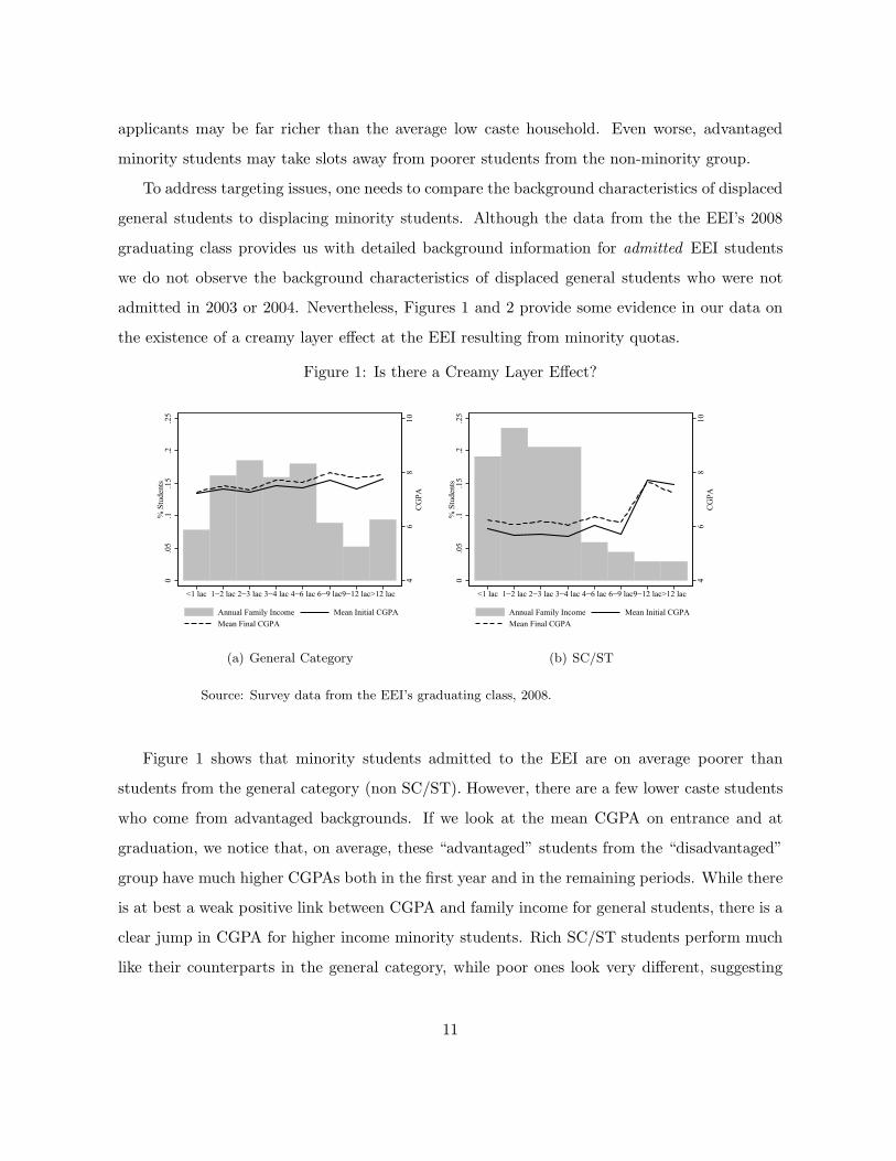
admitted in 2003 or 2004. Nevertheless, Figures 1 and 2 provide some evidence in our data on

the existence of a creamy layer effect at the EEI resulting from minority quotas.

Figure 1: Is there a Creamy Layer Effect?

46

810

CG

PA

0.0

5.1

.15

.2.2

5%

Stu

dent

s

<1 lac 1−2 lac 2−3 lac 3−4 lac 4−6 lac 6−9 lac9−12 lac>12 lac

Annual Family Income Mean Initial CGPAMean Final CGPA

(a) General Category

46

810

CG

PA

0.0

5.1

.15

.2.2

5%

Stu

dent

s

<1 lac 1−2 lac 2−3 lac 3−4 lac 4−6 lac 6−9 lac9−12 lac>12 lac

Annual Family Income Mean Initial CGPAMean Final CGPA

(b) SC/ST

Source: Survey data from the EEI’s graduating class, 2008.

Figure 1 shows that minority students admitted to the EEI are on average poorer than

students from the general category (non SC/ST). However, there are a few lower caste students

who come from advantaged backgrounds. If we look at the mean CGPA on entrance and at

graduation, we notice that, on average, these “advantaged” students from the “disadvantaged”

group have much higher CGPAs both in the first year and in the remaining periods. While there

is at best a weak positive link between CGPA and family income for general students, there is a

clear jump in CGPA for higher income minority students. Rich SC/ST students perform much

like their counterparts in the general category, while poor ones look very different, suggesting

11

that it is the interaction of poverty and SC/ST status that is most harmful.

Figure 2 is consistent with this insight. Panel (a) shows that higher income students from

the general group have slightly higher average grades. However, both first order and second

order stochastic dominance of the distribution of richer general students is rejected. Panel (b)

in Figure 2 shows that high income students among the SC/ST have much higher grades than

low income ones. In addition, while the general category has some rich students with poor

GPAs, the SC/ST does not. A Kolmogorov-Smirnov type test cannot reject the null of second

order dominance of the grade distribution for rich SC/ST students over that for poorer minority

students, which is consistent with the higher mean and lower dispersion for the rich observed

by eyeballing the data.

Figure 2: First Year CGPA Distribution by Caste and Income Level

0.2

.4.6

.8D

ensi

ty

4 5 6 7 8 9 10First Year CGPA

Low Income (<3lac) Middle Income (3−6 lac)High Income (>6 lac)

(a) General Category

0.2

.4.6

.8D

ensi

ty

4 5 6 7 8 9 10First Year CGPA

Low Income (<3lac) Middle Income (3−6 lac)High Income (>6 lac)

(b) SC/ST

Source: Survey data from the EEI’s graduating class, 2008.

Results from a regression of initial CGPA on income, caste, and controls confirm that the

interaction between high income (above 9 lacs) and SC/ST is still positive and significant even

after adding additional regressors and despite very few SC/ST students in the highest income

group (see Table C.2). These results confirm the evidence presented above: poor minority

students start off lagging behind general and rich minority students.

To summarize, better-off minority students who benefit from caste-based preferences repre-

12

sent a very small proportion of all the SC/ST students admitted into the EEI (see histogram in

Figure 1) and they look like students in the general category. These two facts suggest that the

extent of the creamy layer problem at the EEI might be small. However, we must keep in mind

that we are only comparing admitted students across income groups and caste and we know

nothing about general applicants who are not placed due to the minority preferences.

Fortunately, we can learn more about targeting by using the 2009 entrance exam applicant

database (see Appendix D for more details on district-level patterns identified in the 2009 ap-

plicant data). As described in Section 3, admission through the centralized entrance exam is a

deterministic function of the student’s score and caste. Within their caste, students are ranked

according to their exam score and only those above a caste-specific threshold make it into their

group’s merit list. Descending through the caste-specific score ranking, students in each merit

list are progressively placed until all available seats for that caste are filled or until all students

in the merit list are placed. Given this system, we can evaluate the targeting properties of the

AA policy. A basic test would be to compare the economic background of minority students

admitted under the preferences (“displacing” students) to that of students who are denied a

seat but who would have been accepted in the absence of the preferences (“displaced students”).

If displacing students are less advantaged than displaced students we can conclude that AA is

redistributing resources to relatively poorer students.

As mentioned before, the 2009 applicant data lacks of data on final college placement. How-

ever, we approximate displaced and displacing groups using the information on the students in

each caste-specific merit list as well as the number of seats available for each caste group. In

2009, all colleges using the centralized exam to regulate admission offered 8295 seats.15 Out of

these seats, 4784 were assigned to general students, while 1594, 1282, and 635 were reserved for

OBC, SC, and ST students, respectively. We construct the displaced GE group with all general

students who would have obtained a seat in a college (including the EEI) if the 8295 seats were

allocated without caste-specific preferences. These are general students who made it into the

common merit list but who were ranked worse than the 4784th general student in this list and

so ended up without a seat. The displacing SC/ST group consists of two groups: i) SC students

15Additionally, 251 seats were reserved for students with physical disabilities but since we do not have theseapplicants in the applicant data we exclude them from the analysis.

13

who did not qualify into the common merit list but who are better ranked than the 1282nd

student within the SC merit list and ii) ST students who did not qualify into the common merit

list but who are better ranked than the 635th student within the ST merit list. In 2009, 93%

(92%) of the SC (ST) applicants in the SC (ST) merit list are displacing students.16

Figure 3: Does AA Target Students from the Poorest Districts?0

.2.4

.6.8

1C

um. D

ensi

ty

0 20 40 60 80 100% Poor in district of residence (Urban)

Displaced GE Displacing SC/ST

Source: Centralized Entrance Exam, Applicant data 2009.

Assuming that neither the number of applicants in each caste nor the number of seats

available would change in the absence of the AA policy, we can compare district poverty rates

across displaced and displacing groups to evaluate the targeting properties of the program.

Figure 3 plots the cumulative distributions of the percentage of poor in urban areas in the

applicants’ districts of residence for both groups. It is clear that displacing minority students

come from poorer districts compared to displaced general students. The null of first or higher

order stochastic dominance is rejected, but when rich districts with poverty rates below 4% are

dropped, the distribution of poverty rates of displacing students second order dominates that

of displaced students. This suggests that the use of minority admission preferences at the EEI

is effectively redistributing educational opportunities to students who live in poorer districts.

16Although we might mislabel some applicants due to non-enrolment after placement, we expect this potentialbias to be small. Colleges who allocate seats using this centralized exam are top higher education institutions inthe country so students who are offered a seat in one of them are not very likely to reject it.

14

However, lack of individual data on income or consumption in the 2009 applicant database does

not allow us to compare living standards of displacing SC/ST’s households to that of the average

minority household.

5.2 Catch up

The use of minority preferences on college admission in India is justified by the under-representation

of SC and ST students in higher education institutions. AA policies were introduced as a way

to alleviate the legacy of the caste system and allow SC and ST groups to catch up to the

educational and labor outcomes of upper castes. In turn, opponents of affirmative action argue

that reservation schemes undermine the quality of education since the lack of preparation of

minority students during childhood cannot be amended at such a late stage. They argue that

minority students who benefit from preferential admission start off college far behind students

accepted under regular criteria and that competition while in college will then translate into

poor performance among SC and ST students.

Figure 4: Proportion of General and SC/ST Students by 2009 Entrance Exam Score Deciles

0.2

.4.6

.8Pr

opor

tion

of st

uden

ts

1 (lowest) 2 3 4 5 6 7 8 9 10 (highest)

GE OBC SC/ST

Source: Centralized Entrance Exam, Applicant data 2009.

In fact, data on test results for the universe of students taking the exam in 2009 reveal a

huge difference in initial caste-based academic levels. If we look at the distribution of exam

scores in Figure 4, we find that SC/ST students account for 22% of those in the lowest decile.

15

Moreover, their participation in higher deciles steadily declines and their contribution in the

top decile only reaches 3%. In turn, almost 80% of the students in the top decile come from

the general category. Even more striking is the participation of backward castes in the common

merit list: out of the 8,295 students who made it into the common merit list in 2009, only 78

come from SC while 15 come from ST.

But how is the educational gap between general and SC/ST students changing once at the

EEI? First of all, what do we mean by educational gap? One approach might be to look at

how these two groups fare at the end of their time at the EEI relative to the beginning. Figure

5 compares the cumulative GPA of minority and non-minority students at the end of the first

year and by the end of their programs, net of their initial performance. While it is clear that

the distribution of grades among general students always first order dominates that of minority

students (a Kolmogorov-Smirnov type test confirms it), a first look might lead one to think that

SC/ST students are catching up. For both SC/ST and the GE group, the CGPA distribution

at the end seems to improve relative to that in the first year, and more so for minority students.

By this measure, the gap in average CGPA between general and SC/ST students shrinks by

15%.17 But we argue below that this is not comparing like to like as we need to control, at the

very least, for major choices and differences in grading across majors.

Figure 6 presents the evolution of grades over years by caste. Among general students,

the distribution of grades does not move much over time. However, the distribution of grades

for SC/ST students seems to be improving as time in the EEI goes by. While the gap in

average CGPAs between the first and the last year contracts by 10% among general students,

the reduction is close to 15% among minority students.

It is tempting to interpret the evidence in Figures 5 and 6 as preliminary evidence in favor of

catch up, but it is inappropriate to do so without controlling for the major or without taking into

account relative instead of absolute grades. First, if GPAs tend to go up in later semesters, say

because faculty grade more leniently in advanced courses, we could see CGPAs drifting upwards

17Notice that for each time period and caste group, average CGPA is given by the area above the cumulativedistribution. The gap between GE and SC/ST average scores in the first year is just the area between the twosolid curves. Similarly, the gap between the two groups at the end of their careers is the area between the dashedcurves. The contraction of the gap in averages scores is just the percentage change in these areas between thefirst and the last year at the EEI.

16

Figure 5: Performance Gap between GE and SC/ST Students at the EEI

0.2

.4.6

.81

Cum

. Den

sity

4 6 8 10Cumulative GPA

GE, 1st year SC/ST, 1st yearGE, net of 1st year SC/ST, net of 1st year

Source: Survey data from the EEI’s graduating class, 2008.

Figure 6: Evolution of GPA over Time

0.2

.4.6

.81

Cum

. Den

sity

0 2 4 6 8 10CGPA

1st Year 2nd Year3rd Year 4th Year

(a) GE

0.2

.4.6

.81

Cum

. Den

sity

0 2 4 6 8 10CGPA

1st Year 2nd Year3rd Year 4th Year

(b) SC/ST

Source: Survey data from the EEI’s graduating class, 2008.

17

for all students over time. Moreover, if some majors do more of this than others, and SC/ST

students select into these majors, then we might see the above even if there was no catch up.

Finally, if we are interested in catch up, we should not be looking at the absolute grades, but at

the relative grades within each program. In fact, this is exactly what Arcidiacono et al., 2011

show happens in elite U.S. colleges. Although the gap between white and black GPA falls by

half between the first and the last year of college, this comes primarily from switching into easier

majors and smaller variance in grading during later years.

To control for major and relative grades, we look at how students who were in a particular

percentile in terms of first year CGPA, relative to all those in their major, fared in terms of their

CGPA after the first year, relative to all those in their major. If students who were in the 30th

percentile of their major in terms of their first year CGPA are on average in the 40th percentile

in terms of their CGPA in the next 3-4 years of their careers, catch up may be occurring. In turn,

if those students average at the 20th percentile after the first year, they are falling back instead

of catching up. Since we are considering how students fare relative to others in their major, we

eliminate the effect of different grading standards across majors. Moreover, by considering their

ordinal standing rather than the level of CGPA, we eliminate the effect of differences in grades

in early versus late semesters.

Panel (a) in Figure 7 plots average major ranks at graduation versus first year major ranks

both by caste and major selectivity. Average percentiles at the end are calculated through

separate locally linear regressions within each group.18 Thus, for example, general students in

non-selective majors who were in the 20th percentile of their majors in terms of their fist year

CGPA are, on average, in the 28th percentile of their major at graduation, measured in terms

of their final CGPA net of the first year.

In general, the curves presented in Panel (a) show that the slope of the final average ranking

with respect to the initial ranking is less than unity, especially at the top and bottom. This

is to be expected as those initially at the bottom have no place to go but up and those at the

top have no place to go but down. In other words, reversion to the mean should be present.

18To avoid misleading patterns due to outliers, the five SC/ST students who ranked above the 50th percentilein the first year are removed. Two of these dropped observations belong to the group of minority students whohave high family income.

18

Figure 7: Average Ranking at Graduation by Initial Ranking: Major-Specific Percentiles ofCGPA

020

4060

8010

0

Ave

rage

CG

PA p

erce

ntile

at g

radu

atio

nne

t of 1

st y

ear,

rela

tive

to m

ajor

0 20 40 60 80 100First year CGPA percentile, relative to major

GE, Selective SC/ST, SelectiveGE, Non−Selective SC/ST, Non−Selective

(a)−.

50

.51

1.5

GE,Selective

GE,Non−Selective

SC/ST,Selective

SC/ST,Non−Selective

Point Estimate

(b)

Source: Survey data from the EEI’s graduating class, 2008.

Notes: Bachelor programs in CS and EE Power as well as dual degree programs in CS and EE are classified as

Selective Majors. Average final rankings are locally mean-smoothed using a kernel-weighted local polynomial

smoother.

Nevertheless, in the general category, irrespective of the selectivity of the major, these curves

are very close to the 45 degree line suggesting that, on average, general students stay in the

major-specific percentiles they start off in. However, this is not the case for SC/ST students.

Panel (a) shows that the slope for selective and non-selective majors seems to be below one for

minority students and it is even flatter for selective majors, suggesting that SC/ST students are

falling behind over time and more so in more selective majors.

Panel (b) in Figure 7 presents the results of separate regressions by caste and major selectivity

of the final major rank on the initial percentile relative to the major. The round marker shows

point estimates of the coefficient of the initial ranking while the vertical line represents the 95%

confidence interval of each coefficient. The estimates confirm the pattern observed in panel (a):

the slope of final ranking with respect to the initial ranking is close to one for general students,

and even so for SC/ST students in less selective majors. In fact, we cannot reject the null of

19

the coefficient being equal to unity for the latter. In turn, the slope for SC/ST students in more

selective majors is around 0.25 and unity is clearly far outside the confidence interval.

The evidence presented in Figure 7 suggests that the catch up we seemed to find in the

aggregate was an illusion. When we look at how SC/ST students do relative to those in their

major over time, a different picture emerges. Although minority students in less selective majors

are able to at least keep up, SC/ST students in more selective majors seem to be falling behind

rather than catching up. This is not surprising considering that minority students start college

lagging far behind non-minority students. Consequently, the gap between general and SC/ST

students is likely to increase as both groups progress through college, especially in more selective

majors. Even by running as fast as they can, SC/ST students can hope, at best, to stay in the

same place they started but those in more competitive majors cannot even do this and fall even

further behind their general category peers.

5.3 Mismatch

The evidence so far seems to suggest that minority students are not catching up in terms of

academic performance. On the contrary, SC/ST students in more selective majors tend to fall

behind in their major-specific rankings as they progress through college. This pattern seems

to be supportive of the mismatch hypothesis, which predicts lower success rates for minority

students who enrol in more selective colleges and/or majors relative to those in colleges and/or

majors where their academic credentials are better matched to the average.

We first explore the extent to which AA policies motivate minority students to aim for more

selective majors at the EEI. Figure 8 displays the fractions of general and minority students in

the EEI who are accepted into selective majors as functions of their first year CGPA percentile.19

The fraction of students in selective majors at each percentile score is computed from separate

locally linear regressions within each group. Although the fraction of students who attend selec-

tive majors is increasing in initial performance for both general and SC/ST students, minority

students are much more likely to attend selective majors for all levels of first year CGPA. This

evidence is consistent with Rothstein and Yoon’s (2009) findings on school choice for white and

black students in law school and it suggests that the reservation schemes in India are playing a

19Again, the five minority students above the 50th percentile in terms of first year CGPA are dropped.

20

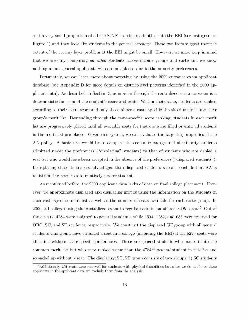
significant role in the major choice of SC/ST applicants.

Figure 8: Fraction of Students Attending Selective Majors by Caste and Initial CGPA Percentile

0.2

5.5

.75

1Fr

actio

n in

sele

ctiv

e m

ajor

s

0 25 50 75 100Percentile CGPA Score in the First Year

GE SC/ST

Source: Survey data from the EEI’s graduating class, 2008.

Notes: Bachelor programs in CS and EE Power as well as dual degree programs in CS and EE are classified as

Selective Majors. Fractions are locally mean-smoothed using a kernel-weighted local polynomial smoother.

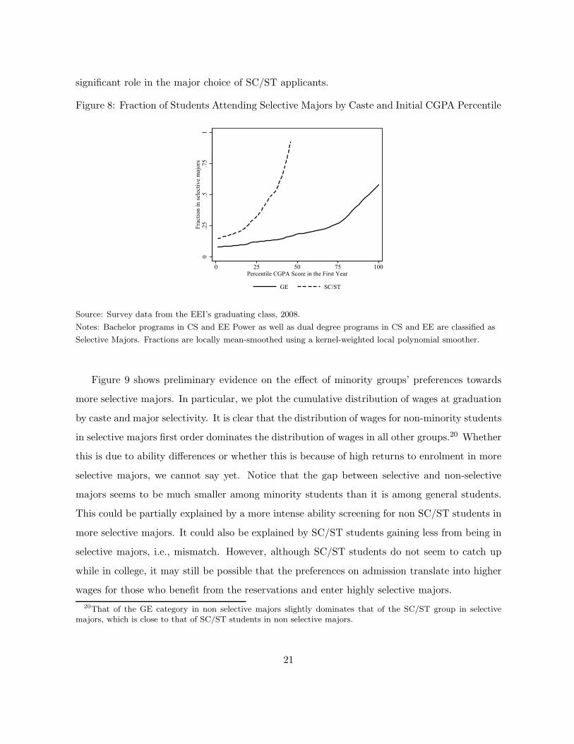
Figure 9 shows preliminary evidence on the effect of minority groups’ preferences towards

more selective majors. In particular, we plot the cumulative distribution of wages at graduation

by caste and major selectivity. It is clear that the distribution of wages for non-minority students

in selective majors first order dominates the distribution of wages in all other groups.20 Whether

this is due to ability differences or whether this is because of high returns to enrolment in more

selective majors, we cannot say yet. Notice that the gap between selective and non-selective

majors seems to be much smaller among minority students than it is among general students.

This could be partially explained by a more intense ability screening for non SC/ST students in

more selective majors. It could also be explained by SC/ST students gaining less from being in

selective majors, i.e., mismatch. However, although SC/ST students do not seem to catch up

while in college, it may still be possible that the preferences on admission translate into higher

wages for those who benefit from the reservations and enter highly selective majors.

20That of the GE category in non selective majors slightly dominates that of the SC/ST group in selectivemajors, which is close to that of SC/ST students in non selective majors.

21

Figure 9: Cumulative Distribution of Wages by Caste and Major Selectivity

0.2

.4.6

.81

Cum

. Den

sity

<3 lac 3−4 lac 4−5 lac 5−7 lac 7−10 lac10−15 lac15−25 lac>25 lac

First Wage after Graduation

GE, Selective SC/ST, SelectiveGE, Non Selective SC/ST, Non Selective

Source: Survey data from the EEI’s graduating class, 2008.

The rest of this sub section will evaluate the effect of major selectivity on labor market out-

comes for both general and SC/ST students. Since admission is only driven by caste and per-

formance in the centralized entrance exam, the allocation of seats in selective and non-selective

majors is not exogenous with respect to future academic performance and wages. Taking into

account that allocation to selective and non-selective majors is not random, we try to assess the

causal link between major selectivity and first wage after graduation.

To evaluate the mismatch hypothesis, we compare the wages of students in selective majors

with their same-caste counterparts in less selective majors. This task requires taking into ac-

count that graduating from a selective major depends on being admitted to that major, which

ultimately depends on ability (maybe partially unobserved) and other individual characteristics

that also determine wages.

Let S∗

i be a latent continuous variable which is increasing in the selectivity of i’s major:

S∗

i = Ziγ − µi

where Zi denotes observed individual characteristics such as gender, first year CGPA (proxy for

entrance exam score), family income, father’s education, school type, a dual degree dummy, and

22

type of job. Define Si = 1 if S∗

i ≥ 0 and Si = 0 if S∗

i < 0. Assuming that µi ∼ N(0, σ2µ), the

probability of being enroled in a selective major is given by:

Pr(S = 1|Zi) = Φ(Ziγ;σ2

µ) (1)

Let w∗

i denote individual i’s log wage at graduation (in logs of lacs):

w∗

i = α1Si +Xiβ1 − εi

where Xi is contained in Zi. Our data gives interval data for wages, so we define a discrete

variable, wi, which will be equal to category Wk if ξk−1 ≤ w∗

i < ξk. We use three wage groups

with known thresholds, ξk, at ξ0 = −∞, ξ1 = log(5), ξ2 = log(7), and ξ3 = ∞. Assuming that

εi ∼ N(0, σ2ε ), and representing the normal cumulative distribution with mean zero and variance

σ2 by Φ(x;σ2), the probability of wi = Wk is given by:

Pr(wi = Wk|Xi) = Pr(ξk−1 ≤ w∗

i < ξk)

= Φ(α1Si +Xiβ1 − ξk−1;σ2

ε )− Φ(α1Si +Xiβ1 − ξk;σ2

ε ) (2)

Our model can be summarized by the system (1)-(2). In particular, the parameter of interest

is α1: if α1 ≤ 0, we cannot reject the mismatch hypothesis for SC/ST students in selective ma-

jors. However, we need to take into account the endogenous selection process that determines

allocation into majors, summarized by (1). Measuring the wage premium of selective majors as

the difference in wages of students in selective and non-selective majors gives a biased picture:

upward bias is likely since observable and unobservable personal traits that make a student more

likely to get into a selective major also make a student more likely to get higher wages. For ex-

ample, students with higher exam scores, measured by first year CGPA, are more likely to be in

selective majors and earn higher wages. If we ignore the role of exam score in selection into ma-

jors, the beneficial effect of major selectivity on wages is overestimated as selective majors have

students with relatively higher scores. If we assume that both εi and µi are uncorrelated random

shocks, so that selection into more selective majors is only driven by observables, propensity

score matching techniques yield an unbiased effect of Si on wages. However, if εi and µi contain

unobserved traits that increase the probability of being in a more selective major and that of

23

getting higher wages, propensity score matching methods yield biased estimates of α1. In this

case, the bias caused by the correlation between εi and µi can be prevented by jointly estimating

(1)-(2).

Assuming selection is exclusively driven by observables, we obtain propensity scores (or the

probability of a student being enroled in a selective major) separately for general and minority

students based on their observable characteristics in Xi as well as additional controls such as

coaching expenditures for the entrance exam, number of household members, and age of the

student. We then include the estimated propensity score as an additional regressor in the wage

equation, assuming that enrolment in selective majors is random with respect to wages once we

control for Xi and the propensity score.21

If we also allow selection into selective majors to be related to students’ unobservable char-

acteristics (i.e., εi and µi are correlated through unobservables), the system in (1)-(2) must be

jointly estimated. Despite the availability of extensive survey data at the student level, we could

not find a good exclusion restriction. Finding an instrument that would only affect the major se-

lectivity equation but not the wage equation was impossible given that the determinants of both

equations overlap a great deal. Therefore, identification comes from the normality assumptions

on the error terms.22

Table 1 summarizes our results (see Table C.3 and C.4 for more details). Column 1 provides

a baseline estimate of α1 when the endogeneity of the major choice is ignored and the wage

equation in (2) is estimated including Si and Xi as regressors. Columns 2 provides estimates

based on propensity score matching methods, where the propensity score has been added to

equation (2) as an additional control.

Among general students, being enroled in a more selective major seems to have a positive

and significant effect even after controlling for selection on observables. Of course, α̂1 is lower

once we control for selection on observables, which is expected if students who enrol in more

selective majors are also more likely to earn higher wages. Propensity score matching methods

21See Rosenbaum and Rubin (1983). Unfortunately, we have interval data on wages. If the outcome variablewere binary or continuous, we could also implement the traditional matching approach which provides a non-parametric estimator of α1 without making assumptions on the relationship between wages and Xi (or Zi).

22We also experimented with instruments. For the GE group, the results were very similar to those relyingon functional form assumptions. The sample size was too small in the SC/ST group for us to consider usinginstruments there.

24

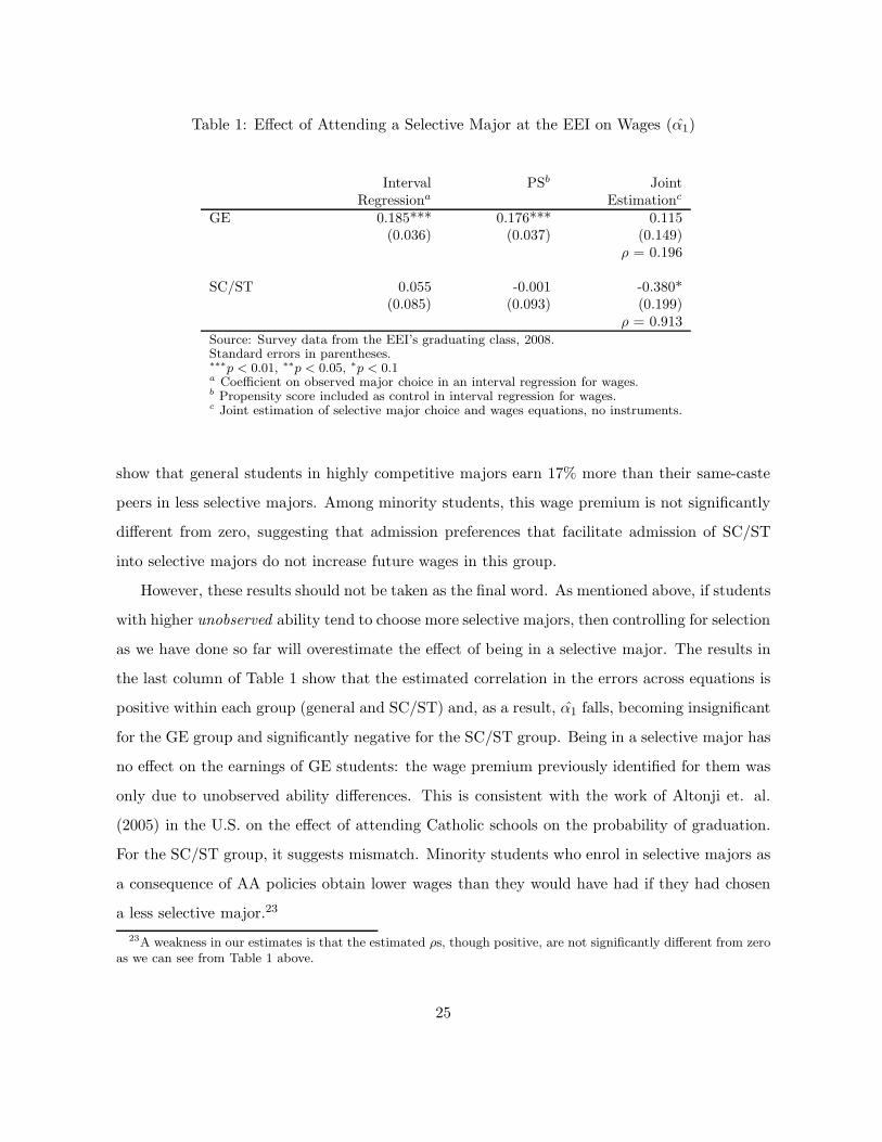
Table 1: Effect of Attending a Selective Major at the EEI on Wages (α̂1)

Interval PSb JointRegressiona Estimationc

GE 0.185*** 0.176*** 0.115(0.036) (0.037) (0.149)

ρ = 0.196

SC/ST 0.055 -0.001 -0.380*(0.085) (0.093) (0.199)

ρ = 0.913Source: Survey data from the EEI’s graduating class, 2008.Standard errors in parentheses.∗∗∗p < 0.01, ∗∗p < 0.05, ∗p < 0.1a Coefficient on observed major choice in an interval regression for wages.b Propensity score included as control in interval regression for wages.c Joint estimation of selective major choice and wages equations, no instruments.

show that general students in highly competitive majors earn 17% more than their same-caste

peers in less selective majors. Among minority students, this wage premium is not significantly

different from zero, suggesting that admission preferences that facilitate admission of SC/ST

into selective majors do not increase future wages in this group.

However, these results should not be taken as the final word. As mentioned above, if students

with higher unobserved ability tend to choose more selective majors, then controlling for selection

as we have done so far will overestimate the effect of being in a selective major. The results in

the last column of Table 1 show that the estimated correlation in the errors across equations is

positive within each group (general and SC/ST) and, as a result, α̂1 falls, becoming insignificant

for the GE group and significantly negative for the SC/ST group. Being in a selective major has

no effect on the earnings of GE students: the wage premium previously identified for them was

only due to unobserved ability differences. This is consistent with the work of Altonji et. al.

(2005) in the U.S. on the effect of attending Catholic schools on the probability of graduation.

For the SC/ST group, it suggests mismatch. Minority students who enrol in selective majors as

a consequence of AA policies obtain lower wages than they would have had if they had chosen

a less selective major.23

23A weakness in our estimates is that the estimated ρs, though positive, are not significantly different from zeroas we can see from Table 1 above.

25

In addition to its effect on wages, being enroled in a more selective major can also affect

minority students’ well-being while at the EEI. Since they see themselves falling behind general

students in the same major they could also be facing higher instantaneous costs of going to college

by being more stressed and frustrated than their same-caste peers in less selective majors.24

We rely on survey data on academic life experience and hostel life to analyze students’ well-

being while in college. In particular, we focus on two survey questions. The first one asks the

students if they had ever felt stressed, depressed, lonely, or discriminated at the EEI where the

possible answers are Never, Occasionally, Often and Regularly. We also rely on a question that

asks the student if he or she felt that the hostel was like a home away from home.

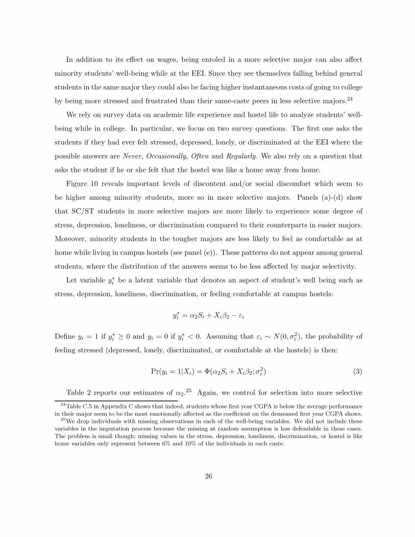
Figure 10 reveals important levels of discontent and/or social discomfort which seem to

be higher among minority students, more so in more selective majors. Panels (a)-(d) show

that SC/ST students in more selective majors are more likely to experience some degree of

stress, depression, loneliness, or discrimination compared to their counterparts in easier majors.

Moreover, minority students in the tougher majors are less likely to feel as comfortable as at

home while living in campus hostels (see panel (e)). These patterns do not appear among general

students, where the distribution of the answers seems to be less affected by major selectivity.

Let variable y∗i be a latent variable that denotes an aspect of student’s well being such as

stress, depression, loneliness, discrimination, or feeling comfortable at campus hostels:

y∗i = α2Si +Xiβ2 − εi

Define yi = 1 if y∗i ≥ 0 and yi = 0 if y∗i < 0. Assuming that εi ∼ N(0, σ2ε ), the probability of

feeling stressed (depressed, lonely, discriminated, or comfortable at the hostels) is then:

Pr(yi = 1|Xi) = Φ(α2Si +Xiβ2;σ2

ε) (3)

Table 2 reports our estimates of α2.25 Again, we control for selection into more selective

24Table C.5 in Appendix C shows that indeed, students whose first year CGPA is below the average performancein their major seem to be the most emotionally affected as the coefficient on the demeaned first year CGPA shows.

25We drop individuals with missing observations in each of the well-being variables. We did not include thesevariables in the imputation process because the missing at random assumption is less defendable in these cases.The problem is small though; missing values in the stress, depression, loneliness, discrimination, or hostel is likehome variables only represent between 6% and 10% of the individuals in each caste.

26

Figure 10: Well-being of the Students While at the EEI

0.2

.4.6

.81

%

Non−selective SelectiveSC/ST GE SC/ST GE

Never Occasionally OftenRegularly Missing

(a) Stress

0.2

.4.6

.81

%

Non−selective SelectiveSC/ST GE SC/ST GE

Never Occasionally OftenRegularly Missing

(b) Depression

0.2

.4.6

.81

%

Non−selective SelectiveSC/ST GE SC/ST GE

Never Occasionally OftenRegularly Missing

(c) Loneliness

0.2

.4.6

.81

%

Non−selective SelectiveSC/ST GE SC/ST GE

Never Occasionally OftenRegularly Missing

(d) Discrimination

01

23

%

Non−selective SelectiveSC/ST GE SC/ST GE

Agree Disagree No view Missing

(e) Hostel does not feel like home

Source: Survey data from the EEI’s graduating class, 2008.

27

Table 2: Effect of Attending a Selective Major at the EEI on Emotional and Social Well-Being(α̂2)

Probita PSb JointEstimationc

StressGE 0.112* 0.125* -0.082***

(0.065) (0.068) (0.010)ρ=0.85

SC/ST 0.351*** 0.320** 0.115**(0.120) (0.137) (0.046)

ρ= -0.34Depression

GE 0.015 0.019 -0.110***(0.052) (0.053) (0.014)

ρ= 0.86***SC/ST -0.249 -0.212 -0.013

(0.152) (0.162) (0.353)ρ= -0.38

LonelinessGE 0.035 0.042 -0.093*

(0.052) (0.054) (0.049)ρ = 0.96

SC/ST -0.089 -0.068 -0.061(0.141) (0.161) (0.109)

ρ = 0.32Discrimination

GE -0.026 -0.026 -0.096**(0.043) (0.045) (0.049)

ρ = 0.68**SC/ST -0.018 -0.018 -0.082

(0.172) (0.212) (0.124)ρ = 0.56

Hostel does not feel like homeGE -0.016 -0.008 -0.003

(0.057) (0.058) (0.085)ρ = -0.01

SC/ST 0.155 0.088 0.121***(0.122) (0.125) (0.036)

ρ=-0.86*Source: Survey data from the EEI’s graduating class, 2008.Standard errors in parentheses.Note: Stress, depression, loneliness, and discrimination dummies are constructed bycoding Often and Regularly as ones. Hostel feels like home dummy is obtained bycoding with ones all students who agree with the statement.∗∗∗p < 0.01, ∗∗p < 0.05, ∗p < 0.1a Coefficient on observed major choice in a probit model.b Propensity score included as control in probit model.c Joint estimation of selective major choice and well-being equations, no instruments.

28

majors using propensity score matching methods and jointly estimating the system (1)-(3).

Once selection into observables and unobservables is taken into account, general students in

more selective majors tend to be slightly happier during their college experience than their

same-race counterparts in less selective majors. The estimated ρs for general students suggest

that more able or motivated students who are more likely to choose tougher majors are also more

likely to face higher levels of emotional discomfort during their college experience.26 Once this

correlation is taken into account, general students in more selective majors are more likely to fit

in socially than non-minority students in less selective majors. However, the story is different

for SC/ST students. Compared to minority students in less selective majors, SC/ST students in

tougher majors are significantly more stressed and feel less comfortable at the hostel facilities.

Mismatch is not only generating lower wages, but it is also imposing a higher cost of going to

college on them.27

In sum, the results suggest that general students do not benefit from being in selective

majors; they earn more because they are better. However, they do tend to face relatively lower

emotional and social costs of studying at the EEI compared to general students in less selective

majors. Taking unobservables into account shows that SC/ST students in selective majors earn

less than minority students in less selective majors, supporting the mismatch hypothesis. These

students also seem to experience what we call social mismatch as they also feel more stressed

and less comfortable at the campus hostels when compared to SC/ST in less selective majors.

5.4 Discrimination in the Labor Market

In the previous sub-section, we found that SC/ST students in selective majors earn less relative

to minority students in easier majors. However, we cannot tell if minority students are better

off as a group due to AA in higher education. Lack of an adequate control group or a structural

model impede us to compare minority students’ wages after graduating from the EEI to their

wages in the absence of minority preferences.

Since we know that very few students from the minority group enter the entrance exam’s

common merit list, it is very likely that without minority preferences most SC/ST students

26The exception is the last variable, hostel does not feel like home, where the correlation is very close to zero.27Social mismatch does not seem to affect wages or grades directly.

29

admitted into the EEI would have gone to a worse school - that is, if they even made it into

college. Given that the Indian labor market rewards degrees from better universities with

higher wages, AA beneficiaries are expected to be better off as a group. However, even if SC/ST

students experience gains from attending the EEI, these benefits could be offset by labor market

discrimination. If employers with negative stereotypes against minority students are less likely

to assign workers from that group to highly rewarded jobs, we could observe discrimination in

terms of wages or occupations (Coate and Loury, 1993). Even worse, if employers are aware of

the extent of minority quotas, coming from the SC/ST group could become a negative signal in

the labor market.

Here we provide some basic evidence on discrimination. We evaluate if, conditional on the

admission minority preferences in place, there is discrimination in the workplace. Although we

are aware of the limitations of a regression-based approach that controls for observable differences

among minority and non-minority students, there is still some informative value in this exercise.

Of course, differences in unobservable traits across groups can bias our estimates.28

Tables C.3 and C.4 showed that the constant term in the wage equation varies very little by

caste, implying that caste-specific mean wages net of observables are very close. Indeed, even

after controlling for selection into majors, grades, and type of job we cannot reject the null that

the constant in the wage equation is equal across groups. But what if discrimination operates

in more subtle ways? We ask below whether SC/ST students seem to get what are seen as less

prestigious or upwardly mobile jobs like those in Finance. Of course, this could be (i) because

such jobs are riskier than jobs using their core competencies in engineering and SC/ST students

are risk averse and choose not to go for such jobs in which case the outcome is benign, or (ii)

because employers are giving SC/ST worse jobs.

To test this hypothesis, we measure occupational differences by caste, conditioning on major

choice and grades. We estimate an ordered probit model where the outcome variable increases as

the job becomes less menial from core and analytical jobs to management/consulting, financial,

28See Charles and Guryan (2011) for more details.

30

and non-technical positions.29 Let j∗i be a continuous latent variable increasing in job’s prestige:

j∗i = α3Si +Xiβ3 − νi

In the data, we find 5 job types, ji, where the first category are core jobs and the last one

corresponds to non-technical positions. The thresholds between categories, ζk, are unknown and

have to be estimated. Again, we assume that νi ∼ N(0, σ2ν) so that the probability of getting a

job in category k is:

Pr(ji = Jk|Xi) = Pr(ζk−1 ≤ j∗i < ζk)

= Φ(α3Si +Xiβ3 − ζk−1;σ2

ν)− Φ(α3Si +Xiβ3 − ζk;σ2

ν) (4)

We estimate the model described by (4) in the complete sample of students but adding a

caste dummy to matrix Xi which is equal to one when the student is from the general group. If

the coefficient for caste in vector β3 turns out to be positive and significant, we argue that there

is some evidence in favor of discrimination against SC/ST graduates in terms of occupation.

Table 3 presents the results for discrimination without controlling for the endogeneity of

major choice, as well as the results that rely on propensity scores and joint estimation of (4)-

(1) to control for selection. When selection into selective majors is ignored, the results from

an ordered probit indicate that initial performance, as measured by the first year CGPA, has

an important positive effect on the probability of getting better jobs. Being from the general

group also seems to have a positive and significant effect on the type of jobs EEI graduates

get. Even after controlling for selection in observables and unobservables, general students get

placed in better occupations relative to comparable SC/ST students but the effect of grades on

job type vanishes. It is worth noting that major selectivity and father’s education turn out to

have a positive and significant effect on job type that persists after controlling for selection in

unobservables. In sum, although there are no earnings differentials by caste within occupations,

the evidence shows that minority students tend to start their labor market experience in less

lucrative occupations which are also less likely to offer professional development opportunities.30

29We order them according to the average wages by occupation in our data.30Notice that the estimated ρ is negative, which implies that students who have higher shocks in the selection

equation also have lower shocks in the type of job equation. In other words, students who prefer more selective

31

Table 3: Occupational Discrimination

Ordereda PSb JointProbit Estimationc

Selective Major 0.194 0.170 1.089***(0.131) (0.136) (0.365)

GE 1.757*** 1.883*** 1.888***(0.208) (0.280) (0.202)

Male 0.097 0.072 0.040(0.172) (0.176) (0.173)

Dual degree/Master 0.132 0.068 -0.009(0.126) (0.158) (0.139)

CGPA First Year (CGPA1) 0.127** 0.058 -0.021(0.055) (0.115) (0.083)

Household Income (base: < 3 lac)[3− 6] lac 0.001 -0.030 -0.064

(0.117) (0.126) (0.119)> 6 lac 0.022 -0.028 -0.084

(0.167) (0.183) (0.171)Father’s Education (base: High School or less)

College or Technical Training 0.252 0.312* 0.356**(0.158) (0.182) (0.159)

Grad Education 0.183 0.220 0.244(0.173) (0.181) (0.171)

School Type (base: Public)KV/Minority -0.068 -0.036 -0.003

(0.243) (0.248) (0.243)Private 0.043 0.042 0.036

(0.154) (0.154) (0.152)Propensity Score 0.469

(0.699)Observations 451 451 451Log likelihood -621.3 -621.1 -831.1ρ -0.535**Source: Survey data from the EEI’s graduating class, 2008.Standard errors in parentheses.∗∗∗p < 0.01, ∗∗p < 0.05, ∗p < 0.1a Coefficient on observed major choice in a ordered probit model.b Propensity score included as control in ordered probit model.c Joint estimation of selective major choice and type of job equations, no instruments.

majors also prefer worse jobs. This is potentially driven by students in selective majors who prefer to work inacademic jobs instead of highly paid jobs in the private sector.

32

6 Conclusion

AA policies always generate divided opinions and provoke intense debate. In the U.S., for exam-

ple, evidence showing that AA policies have only benefited richer black students has promoted

proposals to shift from race-based to economic-based affirmative action. This paper offers evi-

dence that can contribute to the debate on reservation policies in higher education admissions

in India by analyzing the real impact of such policies on their intended beneficiaries.

Using detailed data on the 2008 graduating class from an elite engineering institution (EEI)

in India and applicant data on students taking the joint entrance exam for engineering colleges

in 2009, this article tries to cast some light on the effects of AA on Indian minorities. Our paper

is particularly relevant because it overcomes the limitations of U.S. studies. First, admission

criteria are clear and rigid so that performance in the entrance exam is all that matters to get

into the EEI in contrast to the much more nebulous admissions process in the U.S. Moreover, the

use of AA policies in India results in very large differences in admission standards, which implies

that our empirical results are unlikely to be confounded by the program being a marginal one.

Finally, the strict curricula in higher education Indian institutions minimizes the issue of self

selection into easier courses within a major so that grades are a better indicator of performance.

We provide some basic evidence on three issues central to the debate over AA: targeting,

catch up, and mismatch. We also offer some basic evidence on discrimination. We find that

minority admission preferences seem to be doing a reasonable job targeting poorer populations,

though there seems to be little evidence of catch up. In fact, minority students in more selective

majors seem to be falling behind, suggesting that mismatch effects might be present. Finally,

we find no effect of major selectivity on wages for minority students when only observables are

assumed to drive selection into selective majors. However, when the effect of unobservables

is taken into account, the results suggest that minority students do not benefit from being

in selective majors to which they are attracted by the preferences. In fact, SC/ST students

in selective majors earn less than minority students in less selective majors, supporting the

mismatch hypothesis. Although there are no earnings differentials by caste within occupations,

minority students seem to be placed in worse occupations than general students.

As Rothstein and Yoon (2008) point out, the pervasive nature of affirmative action policies

33

eliminates the possibility of finding a control group for the minorities benefited by the policy.

Rothstein and Yoon (2009) argue that much of the existing evidence on catch up and mismatch is

flawed since differences in the control groups chosen have been an important source of variation

across studies. One of our planned extensions is to develop a structural model that can help us

overcome a difficulty faced by most empirical studies on the topic: finding a control group.

34

References

[1] Allison, Paul. 2001. “Missing Data”. Thousand Oaks, CA: Sage.

[2] Alon, Sigal, and Marta Tienda. 2007. “Diversity, Opportunity, and the Shifting Meritocracyin Higher Education” , American Sociological Review, 72(4) August. 487-511.

[3] . 2005. “Assessing the “Mismatch” Hypothesis: Differences in CollegeGraduation Rates by Institutional Selectivity”, Sociology of Education, 78: 294-315.

[4] Altonji, Joseph G., Todd E. Elder, and Christopher R. Taber. 2005. “Selection on Observedand Unobserved Variables: Assessing the Effectiveness of Catholic Schools”, Journal of

Political Economy, University of Chicago Press, 113(1): 151-184.

[5] Arcidiacono, Peter. 2005. “Affirmative Action in Higher Education: How do Admission andFinancial Aid Rules Affect Future Earnings?”, Econometrica, Vol. 73, No. 5 (September),1477-1524.

[6] . 2011. “What Happens After Enrollment? An Analysis of the Time Pathof Racial Differences in GPA and Major Choice”, Working paper.

[7] Bertrand, Marianne, Rema Hanna, and Sendhil Mullainathan. 2010. “Affirmative Actionin Education: Evidence from Engineering College Admissions in India”, Journal of PublicEconomics, 94(1-2): 16-29 .

[8] Blau, Judith, Stephanie Moller, and Lyle Jones. 2004. “Why test? Talent loss and enrolmentloss”, Social Science Research, 33:40934.

[9] Bowen, William and Derek Bok. 1998. “The Shape of the River”, Princeton UniversityPress.

[10] Carnevale, Anthony P. and Stephen J. Rose. 2003. “Socioeconomic Status, Race/Ethnicityand Selective College Admissions”, The Century Foundation, New York.

[11] Chakravarty, Sujoy and E Somanathan. 2008. “Discrimination in an Elite Labour Market?Job Placements at IIM-Ahmedabad”, Economic and Political Weekly, 43(44): 45-50.

[12] Charles, Kerwin Kofi and Jonathan Guryan. 2011. “Studying Discrimination: FundamentalChallenges and Recent Progress”, The Annual Review of Economics, 3:479–511.

[13] Chaudhuri, Siladitya and Nivedita Gupta. 2009. “Levels of Living and Poverty Patterns: ADistrict-Wise Analysis for India”, Economic and Political Weekly, 44(9): 94-110.

[14] Coate, Stephen and Glenn Loury. 1993. “Will Affirmative-Action Policies Eliminate Nega-tive Stereotypes?”, The American Economic Review, 83(5): 1220-1240.

[15] Kahlenberg, Richard D. (ed). 2004. “America’s Untapped Resource: Low-Income Studentsin Higher Education”, Century Foundation Press, New York.

35

[16] . 1996. “The Remedy: Class, Race, and Affirmative Action”, Basic Books,New York.

[17] Kochar, Anjini. 2010. “Affirmative Action through Quotas: The Effect on Learning InIndia”. Stanford Center for International Development, Working Paper No. 430.

[18] . 1993. “Affirmative Action in Higher Education”, American Economic

Review, American Economic Association, 83(2), pp. 99-103.

[19] Loury, Linda Datcher and David Garman. 1995. “College Selectivity and Earnings”, Journalof Labor Economics, University of Chicago Press, 13(2), pp. 289-308.

[20] National Commission for Enterprises in the Unorganised Sector. 2009. “The Challenge ofEmployment in India An Informal Economy Perspective”, Volume 1.

[21] Rothstein, Jesse M. and Albert Yoon. 2009. “Mismatch in Law School”, Working paper.

[22] . 2008. “Affirmative Action in Law School Admissions: What Do RacialPreferences Do?”, University of Chicago Law Review 75(2), Spring, pp. 649-714.

[23] Sander, Richard H. 2004. “A Systemic Analysis of Affirmative Action in American LawSchools”, Stanford Law Review, 57(2): 367-483.

[24] Van Buuren, S., Brand, J.P.L., Groothuis-Oudshoorn, C.G.M. and Rubin, D.B. 2006. “Fullyconditional specification in multivariate imputation”, Journal of Statistical Computation

and Simulation 76: 1046-1064.

36

A Appendix A: Pattern of missing observations

Table A.1: Summary Statistics

% Missing Original Dataset Imputed DatasetVariable (N=453) Mean S.D. Mean S.D.Male 0.0 0.90 0.90General Category 0.0 0.85 0.85First year CGPA 0.0 7.20 1.17 7.20 1.17CGPA at graduation 0.0 7.40 1.03 7.40 1.03Bachelor’s degree (Dual/Master’s = 0) 0.0 0.79 0.79Major

CS 0.0 0.13 0.13ME 0.0 0.20 0.20EE 0.0 0.17 0.17CH 0.0 0.13 0.13BB 0.0 0.05 0.05MT 0.0 0.04 0.04PH 0.0 0.06 0.06TT 0.0 0.09 0.09CE 0.0 0.12 0.12

Family income (lac) 1.8<1 0.09 0.101-2 0.17 0.172-3 0.19 0.193-4 0.17 0.174-6 0.16 0.166-9 0.08 0.089-12 0.05 0.05>12 0.08 0.08

Number of household members 2.4 2.22 0.75 2.25 0.82Enter the EEI in first attempt 3.1 0.49 0.49Father’s occupation 3.5

Non main earner - retired 0.05 0.08Government or public sector 0.54 0.52Private sector 0.42 0.40

Mother’s occupation 3.5Non main earner - house wife 0.71 0.72Government or public sector 0.17 0.17Private sector 0.12 0.11

Father’s education 5.3Middle school or less 0.04 0.09High school 0.10 0.09College 0.53 0.50Post-graduate 0.34 0.32

Mother’s education 5.3Middle school or less 0.11 0.14

(continues)

37

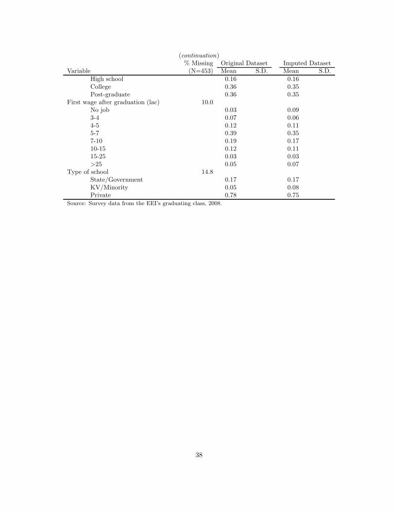
(continuation)% Missing Original Dataset Imputed Dataset

Variable (N=453) Mean S.D. Mean S.D.High school 0.16 0.16College 0.36 0.35Post-graduate 0.36 0.35

First wage after graduation (lac) 10.0No job 0.03 0.093-4 0.07 0.064-5 0.12 0.115-7 0.39 0.357-10 0.19 0.1710-15 0.12 0.1115-25 0.03 0.03>25 0.05 0.07

Type of school 14.8State/Government 0.17 0.17KV/Minority 0.05 0.08Private 0.78 0.75

Source: Survey data from the EEI’s graduating class, 2008.

38

B Appendix B: Multiple Random Imputation

Allison (2001) proposes multiple imputation methods as an alternative to maximum likelihoodfunction methods. Like maximum likelihood, multiple imputation estimates are consistent andasymptotically normal and close to being asymptotically efficient. In addition, multiple imputa-tion has two big advantages over maximum likelihood: i) it can be applied to any kind of dataor model and ii) the imputation procedure can be implemented using conventional software.Since imputed values are random draws, the major disadvantage of multiple imputation is thatit produces different imputed databases every time you use it.

The most widely-used method for multiple imputation is the Markov Chain Monte Carloalgorithm based on linear regression. However, in the case of the EEI data, important com-plications arise from the fact that some of the missing variables are categorical. The MonteCarlo method presumes that every variable with missing data is normally distributed and thatis clearly not the case for categorical variables. An alternative approach is known as “sequentialgeneralized regression” or “multiple imputation for chained equations” (MICE). Instead of as-suming a single multivariate model for all the data, this method specifies a separate regressionmodel for each variable which is used to impute missing values. This method is thus flexible andallows us to incorporate logistic, binomial, or multinomial models for categorical variables.31

Each model is estimated sequentially using available data, starting with the variable thathas the fewest missing data and proceeding to the variable with the most missing data. Aftereach model is estimated, the parameter estimates are used to generate imputed values. Onceimputed values have been generated for all the missing data, the sequential imputation processis repeated, except now the imputed values of the previous round are used as predictors forimputing other variables. The main drawback of sequential generalized regressions is that notheory guarantees convergence to the correct distribution for the missing values. However,simulation based evidence in Van Buuren et al. (2006) suggests that the method works well.

The MICE method is implemented in the following way:

1. For each dependent variable to be imputed, choose a model that reflects the type of data.

2. First round: Imputation starts with dependent variable with the fewest missing data andproceeds to dependent variable with the most missing data.

• Order dependent variables according to amount of missing data from Y1 to Yk. Denotevariables with complete data values as X.

• Regress Y1 on X and obtain β̂ and V̂ (β̂). Generate imputed values using observedcovariates and coefficients drawn from N(β̂,V̂ (β̂)).

• Regress Y2 on X and Y1 (including imputed values of Y1) and obtain imputed values.

• Continue until all regression models have been estimated.

3. Second and subsequent rounds repeat the process, but each variable is regressed on all

other variables, using imputed values from previous rounds.

4. Process ends when stable imputed values are reached or after a specified number of rounds.

31See Allison (2001).

39

C Appendix C: Additional Tables and Figures

Table C.1: Average First Year CGPA by Major and Caste

Major Total GE SC/STBachelor’s

Computer Science 8.20 8.56 6.65Electrical Engineering, Power 7.70 8.03 6.37Mechanical Engineering, Production 7.39 7.72 5.59Electrical Engineering 7.32 7.74 5.99Mechanical Engineering 7.26 7.57 5.50Civil Engineering 6.94 6.94Engineering Physics 6.89 6.90 6.44Chemical Engineering 6.75 7.19 5.31Textile Technology 6.69 7.01 5.19

Dual degreeComputer Science 8.09 8.21 6.79Electrical Engineering 7.26 7.31 6.50Chemical Engineering 7.20 7.36 5.25Biotechnology 6.92 7.08 5.48Mathematics and Computing (Master’s) 6.45 6.54 5.87

Source: Survey data from the EEI’s graduating class, 2008.

40

Table C.2: First Year CGPA as a Function of Income and Caste

First YearCGPA

Constant 7.517***(0.205)

Selective Major 0.832***(0.104)

Male -0.402***(0.148)

Dual degree/Master -0.314***(0.109)

SC/ST -1.545***(0.168)

Household Income (base: < 3 lac)[3− 9] lac 0.167

(0.107)> 9 lac 0.194

(0.149)Household Income x Caste

[3− 9] lac x SC/ST -0.349(0.271)

> 9 lac x SC/ST 1.367***(0.516)

Father’s Education (base: High School or less)College or Technical Training 0.053

(0.130)Grad Education -0.052

(0.143)School Type (base: Public)

KV or Minority -0.141(0.194)

Private 0.070(0.129)

Observations 451R-squared 0.383Source: Survey data from the EEI’s graduating class, 2008.

Standard errors in parentheses.∗∗∗p < 0.01, ∗∗p < 0.05, ∗p < 0.1.

41

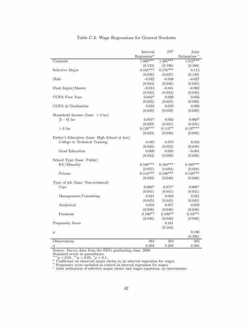
Table C.3: Wage Regressions for General Students

Interval PSb JointRegressiona Estimation c

Constant 1.060*** 1.205*** 1.012***(0.133) (0.196) (0.166)

Selective Major 0.185*** 0.176*** 0.115(0.036) (0.037) (0.149)

Male -0.032 -0.048 -0.027(0.043) (0.046) (0.045)

Dual degree/Master -0.013 -0.041 -0.002(0.032) (0.042) (0.040)

CGPA First Year 0.043* 0.020 0.056(0.025) (0.035) (0.036)

CGPA at Graduation 0.033 0.033 0.028(0.028) (0.028) (0.030)

Household Income (base: < 3 lac)[3− 6] lac 0.055* 0.043 0.060*

(0.029) (0.031) (0.031)> 6 lac 0.129*** 0.112** 0.137***

(0.043) (0.046) (0.046)Father’s Education (base: High School or less)

College or Technical Training 0.045 0.078 0.032(0.040) (0.052) (0.049)

Grad Education 0.009 0.034 -0.001(0.043) (0.050) (0.048)

School Type (base: Public)KV/Minority 0.160*** 0.164*** 0.160***

(0.057) (0.058) (0.058)Private 0.144*** 0.136*** 0.148***

(0.039) (0.040) (0.040)Type of job (base: Non-technical)

Core 0.069* 0.071* 0.068*(0.041) (0.041) (0.041)

Management/Consulting 0.021 0.024 0.021(0.045) (0.045) (0.045)

Analytical 0.058 0.057 0.058(0.046) (0.046) (0.046)

Financial 0.106** 0.106** 0.107**(0.046) (0.046) (0.046)

Propensity Score 0.181(0.182)

ρ 0.196(0.396)

Observations 383 383 383σ 0.203 0.203 0.204

Source: Survey data from the EEI’s graduating class, 2008.Standard errors in parentheses.∗∗∗p < 0.01, ∗∗p < 0.05, ∗p < 0.1.a Coefficient on observed major choice in an interval regression for wages.b Propensity score included as control in interval regression for wages.c Joint estimation of selective major choice and wages equations, no instruments.

42

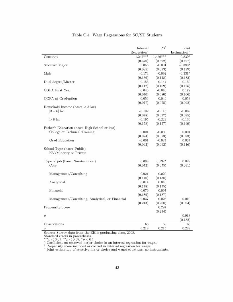
Table C.4: Wage Regressions for SC/ST Students

Interval PSb JointRegressiona Estimation c

Constant 1.247*** 1.459*** 0.830*(0.370) (0.392) (0.497)

Selective Major 0.055 -0.001 -0.380*(0.085) (0.093) (0.199)

Male -0.174 -0.092 -0.331*(0.136) (0.148) (0.182)

Dual degree/Master -0.155 -0.144 -0.159(0.112) (0.109) (0.125)

CGPA First Year 0.046 -0.010 0.172(0.070) (0.080) (0.106)

CGPA at Graduation 0.056 0.049 0.053(0.077) (0.075) (0.092)

Household Income (base: < 3 lac)[3− 6] lac -0.102 -0.115 -0.069

(0.078) (0.077) (0.095)> 6 lac -0.195 -0.223 -0.136

(0.158) (0.157) (0.199)Father’s Education (base: High School or less)

College or Technical Training 0.001 -0.005 0.004(0.074) (0.073) (0.093)

Grad Education -0.001 -0.024 0.037(0.092) (0.092) (0.116)

School Type (base: Public)KV/Minority or Private

Type of job (base: Non-technical) 0.098 0.132* 0.028Core (0.072) (0.075) (0.091)

Management/Consulting 0.021 0.029(0.140) (0.138)

Analytical 0.014 0.010(0.178) (0.175)

Financial 0.079 0.097(0.189) (0.187)

Management/Consulting, Analytical, or Financial -0.037 -0.026 0.010(0.213) (0.208) (0.094)

Propensity Score 0.297(0.214)

ρ 0.913(0.182)

Observations 68 68 68σ 0.219 0.215 0.289

Source: Survey data from the EEI’s graduating class, 2008.Standard errors in parentheses.∗∗∗p < 0.01, ∗∗p < 0.05, ∗p < 0.1.a Coefficient on observed major choice in an interval regression for wages.b Propensity score included as control in interval regression for wages.c Joint estimation of selective major choice and wages equations, no instruments.

43

Table C.5: Well-being as a Function of Relative Academic Disadvantage and Controls

Stressed Depressed Lonely Discriminated Hostel feelslike home

Selective Major 0.005 -0.114 -0.161** -0.106* 0.003(0.089) (0.075) (0.071) (0.060) (0.077)

Male -0.072 -0.024 0.012 0.003 -0.115(0.081) (0.070) (0.067) (0.054) (0.076)

Dual degree/Master 0.047 0.064 0.079* 0.038 0.025(0.060) (0.049) (0.047) (0.037) (0.054)

CGPA First Year (CGPA1) 0.120 0.078 0.158** 0.035 -0.061(0.082) (0.068) (0.066) (0.053) (0.072)

GE 0.069 -0.076 0.193 0.020 -0.046(0.136) (0.105) (0.136) (0.093) (0.126)

(CGPA1 - Major’s mean CGPA1) -0.194* -0.103 -0.296*** -0.095 0.099(0.113) (0.090) (0.097) (0.073) (0.101)

GE x (CGPA1 - Major’s mean CGPA1) -0.012 -0.032 0.052 0.021 -0.052(0.091) (0.070) (0.083) (0.059) (0.080)

Household Income (base: < 3 lac)[3− 6] lac -0.016 -0.040 0.026 0.025 -0.020

(0.053) (0.043) (0.042) (0.034) (0.047)> 6 lac 0.046 -0.016 -0.052 0.039 -0.115*

(0.076) (0.063) (0.065) (0.049) (0.063)Father’s Education (base: High School or less)

College or Technical Training 0.080 0.005 -0.024 0.039 0.003(0.069) (0.055) (0.055) (0.047) (0.060)

Grad Education -0.005 -0.033 0.050 0.043 -0.001(0.076) (0.061) (0.059) (0.051) (0.066)

School Type (base: Public)KV/Minority -0.096 -0.018 -0.174* 0.027 -0.025

(0.100) (0.079) (0.094) (0.053) (0.082)Private 0.029 0.026 -0.031 -0.040 -0.007

(0.066) (0.053) (0.052) (0.039) (0.056)

Observations 422 413 420 412 425Log likelihood -270.5 -194.5 -189.4 -128.8 -226.0

Source: Survey data from the EEI’s graduating class, 2008.Standard errors in parentheses.∗∗∗p < 0.01, ∗∗p < 0.05, ∗p < 0.1.

44

D Appendix D: 2009 Entrance Exam Applicant Data

In general, Figure D.1 shows that there are greater concentrations of exam applicants in northeastern areas, especially in richer districts. Moreover, central regions of the country with higherurban poverty rates are contributing less to the applicant pool. Although this evidence issuggestive, we need to take into account the population “at risk” of taking the exam in eachdistrict to check if certain district characteristics are related to a relatively higher proportionof high school graduates taking the entrance exam. We approximate the probability of takingthe entrance exam in a given district as the number of 2009 applicants from a given PIN codedivided by the number of high school students enroled in grades 9th through 12th in 2006.32

Even though the 2009 applicant data does not contain information about students’ placement,we code all students who made it into their respective merit list and are ranked above themaximum number of seats available for their group as admitted students. We can then proxythe district’s probability of getting into college as the number of admitted students divided bythe total number of applicants from the corresponding PIN code.

Using the results from non-parametric locally linear regressions in the sample of districtswith exam applicants in 2009, Figure D.2 plots districts’ probability of taking the exam and theprobability of getting into college as functions of urban poverty rates, share of rural populationand share SC/ST population. The blue lines in panels (a) and (b) show that both the probabilityof taking the college entrance exam and the probability of getting in do not seem to be affectedby the share of minority population in the district. This pattern is particularly interesting if onetakes into account that areas with higher concentrations of SC/ST population tend to have loweraverage performance in the entrance exam (both in the aggregate and by subject) as shown inpanel (a), Figure D.3. In the absence of AA policies, the lower prospects of success in the examin areas with higher concentrations of minority population would lead to a lower probability oftaking the exam as well as lower chances of being admitted. The fact that we do not identify arelationship between the district’s share of SC/ST population and the probabilities of writing theexam or getting in suggests that admission preferences particularly motivate minority studentsto take the exam and facilitate their admission into college.

When we order districts by their poverty rate, panel (a) in Figure D.2 shows a modest declinein the probability of taking the exam as the percentage of urban poor rises. However, the blackline in panel (b) suggests that there is no relationship between the probability of getting inand poverty. This could be due to preferences for SC/ST who tend to be poorer than the GEgroup. The small differences in the proportion of people getting in may follow from the smalldifferences in average performance among poor and rich districts exhibited in panel (b) in FigureD.3. Finally, the gray lines in panels (a) and (b) in Figure D.2 show that the probability oftaking the exam and the probability of getting into college are both decreasing in the share ofrural population, which reflects AA’s lack of focus on rural students.

32The latter comes from the State Profile 2005-06 prepared by the Indian Ministry of Human Resource andDevelopment. We acknowledge that the total population “at risk”of taking the exam will be overestimated,especially due to higher dropout in the last years of high school, and more so in poorer districts. Unfortunately,data for 12th grade enrolment in 2008 was not publicly available at the district level, only at the state level.

45

Figure D.1: District-Level Poverty Rate and Number of Exam Applicants

Legend

1 Dot = 20

N

% Urban Poor

[0 - 10]

]10 - 25]

[25 - 50]

[50 - 75]

]75 - 100]

missing data

Number of Applicants

Source: Centralized Entrance Exam, Applicant data 2009. Poverty rates from and Chakravarty and

Somanathan (2008).

46

Figure D.2: Probability of Taking the Entrance Exam and Probability of Admission0

.005

.01

.015

.02

Prob

abili

ty o

f tak

ing

the

JEE

0 20 40 60 80 100%

By poverty rate By rural populationBy share of SC/ST

(a) Probability of taking Exam

0.0

1.0

2.0

3.0

4.0

5Pr

obab

ility

of A

dmis

sion

0 20 40 60 80 100%

By poverty rate By rural populationBy share of SC/ST

(b) Probability of Admission

Source: Centralized Entrance Exam, Applicant data 2009.

Note: Probabilities are locally mean-smoothed using a kernel-weighted local polynomial smoother.

Figure D.3: District Average Total Marks and Marks by Subject in the 2009 Entrance Exam

02

46

810

Ave

rage

Mar

ks in

the

Dis

trict

(100

scal

e)

0 10 20 30 40Share of SC/ST Applicants in the District

Total Marks MathChemistry Physics

(a) SC/ST Share

02

46

810

Ave

rage

Mar

ks in

the

Dis

trict

(100

scal

e)

0 20 40 60 80 100% of Urban Poor in the District

Total Marks MathChemistry Physics

(b) Poverty

Source: Centralized Entrance Exam, Applicant data 2009.

Note: Average Marks in panel (a) are locally mean-smoothed using a kernel-weighted local polynomial smoother.

47