Embed Size (px)
Citation preview
AFIT/GOR/OS/85 I)- "jIOTC ALE COPY
tO
II
ASf EL.'CTESEP 3 0 1987
A COST MODEL OF ITEM MIGRATION"IN THE
AIR FORCE LOGISTICS COMMANDCONSUMABLF ITEM INVENTORY
THESIS
Lee J. LohmkuhlCaptain, USAF
AFIT/GOR/OS/BsD-7
Approv*- d . : .. '
S D D Jt .ti---n . - -- --

UNCLASSIFIED - ,SECURITY CLASSIFICATION OF THIS PAGE -
Form ApprovedREPORT DOCUMENTATION PAGE OMiloN oo.-o0eO
4. REPORT SECURITY CLASSIFICATION lb RESTRICTIVE MARKINGS
UNCLASSIFIED2a. SECURITY CLASSIFICATION AUTHORITY 3. DISTRIBUIION/AVAILABILITY OF REPORT
R I... .. Approved for public release;2b. DECLASSIFICATION/DOWNGRADING SCHEDULE distribution unlimited
4. PERFORMING ORGANIZATION REPORT NUMBER(S) S. MONITORING ORGANIZATION REPORT NUMBER(S)
AFIT/GOR/OS/86D-7
68. NAME OF PERFORMING ORGANIZATION 6b. OFFICE SYMBOL 7a. NAME OF MONITORING ORGANIZATION(f applicable)
School of Engineering AFIT/EN
6c. ADDRESS (City, State, and ZIP Code) 7b. ADDRESS (City, State, a•d ZIP Code)Air Force Institute of TechnologyWright-Patterson AFB, Ohio 45433
GB. NAME OF FUNDING/SPONSORING Bb. OFFICE SYMBOL 9. PROCUREMENT INSTRUMENT IDENTIFICATION NUMBERORGANIZATION (If applicable)
Sc. ADDRESS(City, State, and ZlPCode) 10. SOURCE OF FUNDING NUMBERS
PROGRAM PROJECT TASK WORK UNITELEMENT NO. NO. NO ACCESSION N
11. TITLE (irclude Security Classitication)
See Block 19
12. PERSONAL AUTHOR(S)Lehmkuhlf Lee J.( B.S.t M.S.I C_ t USA
13a. TYPE OF REPORT t13b TIME COVERED f14. DATE OF REPORT (Year, Month Day) lS. PAGE COUNT
MS Thesis FROM _ ___TO. 96Dcmp 18116. SUPPLEMENTARY NOTATION
17. COSATI CODES " 18 SUBJECT TERMS (Continue on reverse If necessary and identify by block number)
FIELD GROUP SUB-GROUP Inventory Control, Supply Depots, Economic Order11i 05 Quantity, Markov Processes
19. ABSTRACT (Continue on reverse If necessary and identify by block namber)
TITLE: A Cost Model of Item Migration in the Air ForceLogistics Command Consumable Item Inventory(Unclassified)
Thesis Advisors: Major Joseph R. LitkoDr. Palmer W. Smith $#bd'dk S*, a
p... ..All rylaq Insftitto of Tachnlviov.+[lJbt-~m Atis• OU O L OS1•
20 DISTRIBUTION/ AVAILABILITY OF ABSTRACT 21. ABSTRACT SECURITY CLASSIFICATIONUUNCLASSIrIED/UNLIMITED -1 SAME AS RPT. C DTIC USERS UNCLASSIFIED
22a. NAME OF RESPONSIBLE INDIVIDUAL 122b. I'ELEPHONE (Include Area Code) 22c OFFICE SYMBOLMajor Joseph R. Litko (513) 255-3362 I AFIT/ENS
DD Form 1473, JUN 86 Previous editions are obsolete. SECURITY CLASSIFICATION OF THIS PAGE_.

AFIT/GOR/OS/860-7
A COST MODEL OF ITEM MIGRATION IN THE
AIR FORCE LOGISTICS COMMAND
CONSUMABLE ITEM INVENTORY
THESI S
Presented to the Faculty of the School of Engineering
oF the Air Force Institute of Technology
Air University
In Partial Fulfillment of the
Requirements for thm Degree of
Master of Science
94. co DTIC, TAU
Lee J. Lehmkuhl, B.S. B
Captain, USAF ~-
December 1986
Approved for public release; distribution unlimited
trLqua&
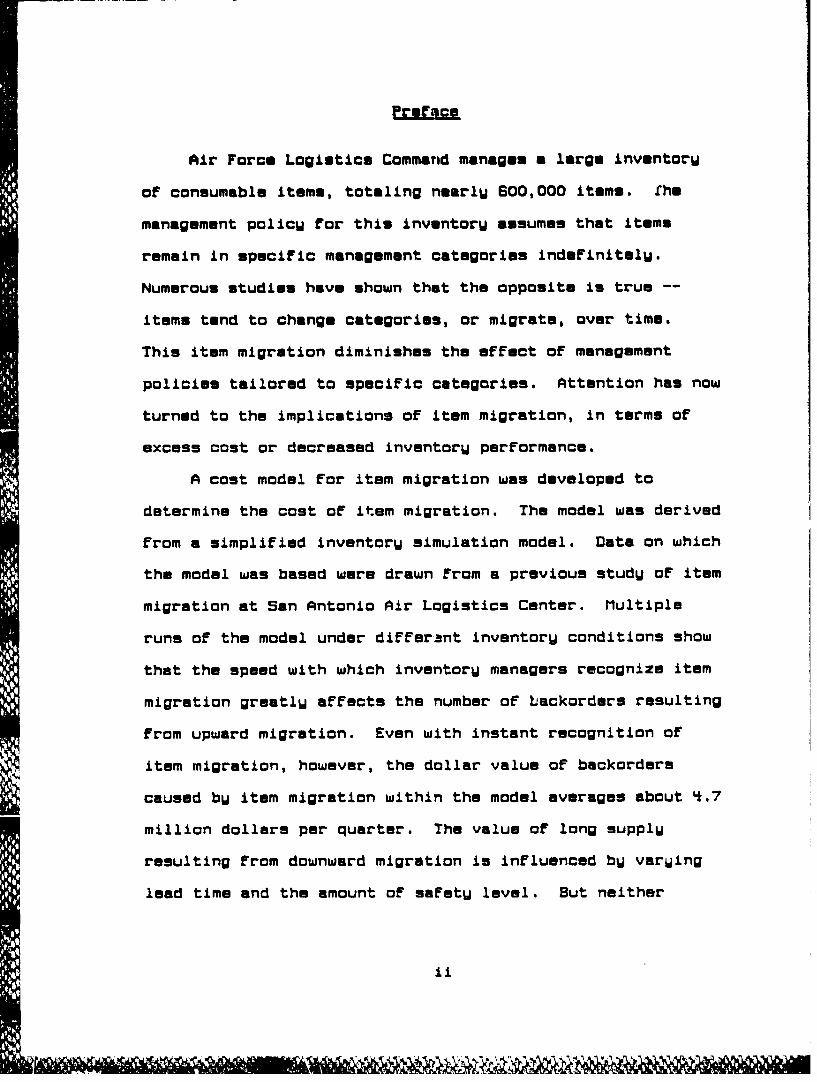
Air Force Logistics Command manages a large inventory
of consumable items, totaling nearly 600,000 items. the
management policy for thiu inventory ausumes that items
remain in specific management categories indefinitely.
Numerous studies have shown that the opposite is true --
items tend to change categories, or migrate, over time.
This item migration diminishes the effect of management
policies tailored to specific categories. Attention has now
turned to the implications of item migration, in terms of
excess cost or decreased inventory performance.
A cost model for item migration was developed to
determine the cost of item migration. The model was derived
from a simplified inventory simulation model. Data on which
the model was based were drawn from a previous study of item
migration at San Antonio Air Logistics Center. Multiple
runs of the model under diFferant inventory conditions show
that the speed with which inventorU managers recognize item
migration greatly affects the number of backorders resulting
from upward migration. Even with instant recognition of
item migration, however, the dollar value of backorders
caused by item migration within the model averages about 4.7
million dollars per quarter. The value of long supply
resulting from downward migration is influenced by varying
lead time and the amount of safety level. But neither

influence is strong enough to greatly affect the total value
of long supply, which averaged about 75 million dollwrs.
This study would not have been possible without the
help of several dedicated people. Mark Fruman, Patti Moore,
and Frsd Rmxroad provided much-needed insight into the AFLC
data bass and item management policy. Special thanks go to
my advisor, Maj Joseph R. Litko, for his suggestions, ideas,
and support; and Lt Col Palmer W. Smith, USAF (Rat), for
giving me a solid foundation in this area and staying with
the project. Finally, I thank mu wifa Michel for her
unfailing support and caring during mu tour at AFIT.
i ils
TIable Contents
-I
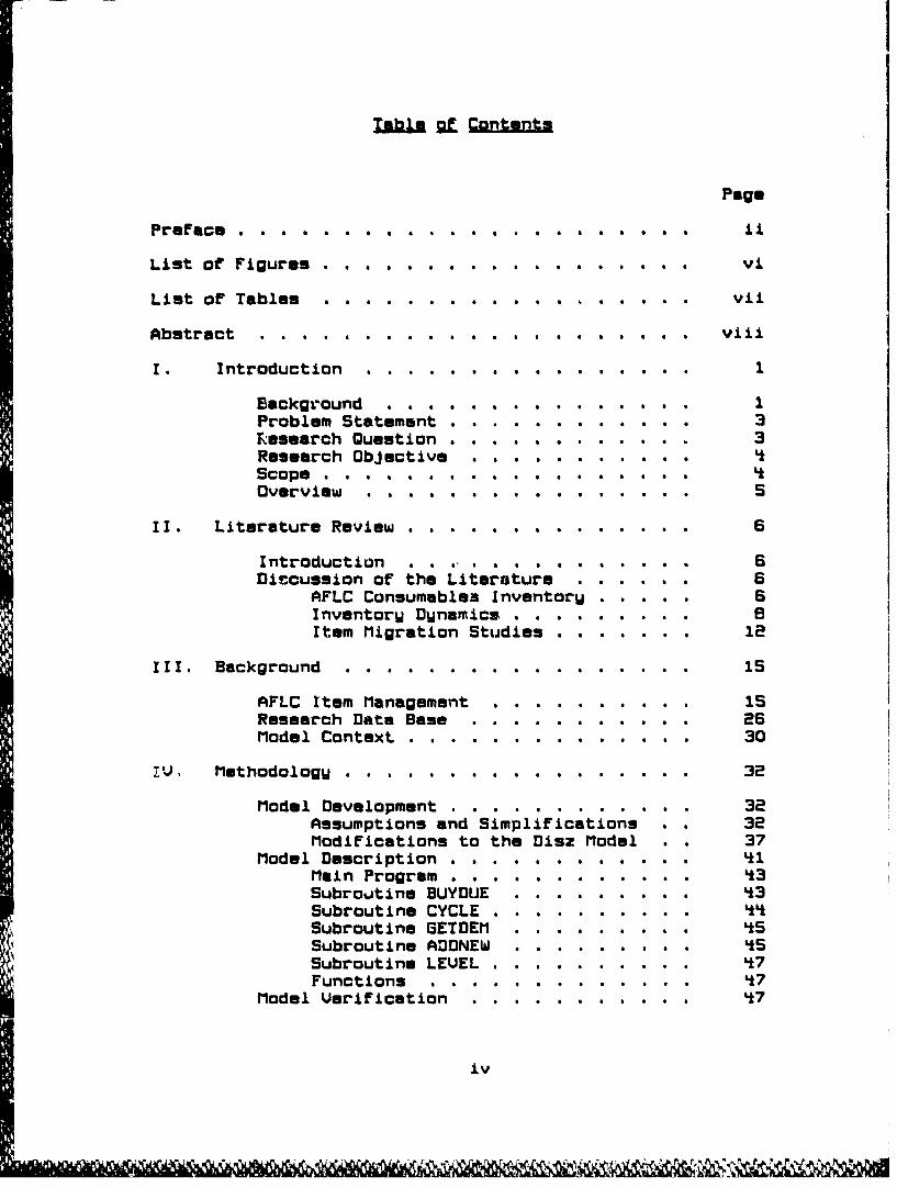
PagePreface . . . . . . . . . .
List of Figures . ....... . ..... ... vi
List of Tables . . . . . . . . . . . . . . . . . vii
Abstract . . . . . . . . . . . . . a a a a viii
I. Introduction . . . . . . . . . . . . . . . ..
Background . . . . . . . . . . . . . . . 1Problem Statement. .... ...... . 3Research Question. .. ........ 3Research Objective . . . . . . . . . . .Scope . . . . . . . . . . . . . . . .
Overview . . . . . . . . . . . . . . . . 5
II. Literature Review . ............ 6
Introduction . . .. . . . . . . . . . . . 6Discussion of the Literature . . . . . . 6
AFLC Consumables Inventory . . . . . 6Inventory Dynamics .........Item Migration Studies . . . . . . . 12
III. Background . . . . . . . . . . . . . . . . . 15
AFLC Item Management ... 9.9.... 15Research Data Base ........... 26Model Context . ........ 9... 30
iv, Methodology . . . . . . . . . . . . . . . . 32
Model Development ..... 32Assumptions and Simplification!s 32Modifications to the Disz Model 37
Model Description.. ........ .1Main Program ... .... .. 3Subroutine BUYDUE ...... . 3Subroutine CYCLE .......... 44Subroutine GETDEM . . . . . . . . . 55Subroutine ADDNEW . . . . . . . . . 54
4 Subroutine LEVEL .......... 47Functions . . . ........... ......... 47
Model Verification .. 7
iv
Model Validation . . . . . . . . . . . . 4 8Steady State Solution . . . . . . . 49Inventory Performance . . . . . . . 51Altered Transition Matrix . . . . . Se
Experimental Design . . . . . . . . . . 53Factors . . . . . . . . . . . . . .Treatments ..... ..... .. . 5
U. Analysis of Results ......... . .. 57
Dollar-Weighted Maximum Backorders . . . S7Analysis of Variance . . . . . . . . 58Comparison of Mean Responses . . . . 60
Dollar Value of Long Supply . . . . . . . 63Analysis of Variance . . . . . . . 60Comparison of Mean Responses . . . . 67
The Cost of Item Migration . . . . . . 70Dollar-WeightedMaximum Backorders . . . . . . . . . 70Dollar Value of Long Supply . . . . 71
UI. Conclusions and Recommendations . . . . . . . 73
Conclusions. ..... . . . . . . . . 73Recommendations...... . . . . . . . 77
Appendix A: MIBSIM FORTRAN Source Cede . . . . . 80
Appendix B: MISSIM Output Reports . . . . . . . S5
Appendix C: MISSIM Output Reports withNo Item Migration . . . . . . . . 146
Appendix D: MIGSIM Output Reports with
Altered Transition Matrix . . . . 148
Appendix E: SAS Residual Plots . . . . . . . . . 164
Bibliography . . . . . . . . . . . . . . . . . . . 165
V
- ~ ~ ~ V t .~~ .Uf&M- .l~~ t .M .lj ' .". i. .~ .) . .~ . X'~ . 7
Figure L=2.Fiue Page
2.MgainTransition Matrix . . . .. ee
3. Assignment of Prices to New Items . . . .. . . 4*0
Lt. Altered Transition Matrix . . . . . . . . . . . S
vi
LIU~ gL Tables
Table Page
I. Steady State Proportions . . . . . . . . . . 50
II. Normalized Steady State vs. ActualSMOC Proportions . . . . . . . . . . . . . 50
III. Normalized Steady State vs. ActualSMIC Proportions . . . . . . . . . . . . . 53
IV. Treatments For Full Factorial Design . . . . 55
U. First Run Dollar-Weighted
Maximum Backorders . ......... . . . 57
UI. Full Model ANOUA Table for Backorders . . . . 55
UII. Reduced Model ANOUA Table for Backorders . . 50
UIII. Mean Responses for Backorders . . . . . . . . 61
IX. First Run Dollar Valum of Long Supply . . . . 6
X. Full Model ANOUA Table for Long Supply . . . 65
XT. Reduced Model ANOVA Table for Long Supply . , 66
XII. Mean Responses for Long Supply . . . . . . 68
vii

This i•wt investigates the phenomenon of
item migration within the Air Force Logistics Command CAFLC)
consumable item tnventory. Item migration is the movement
of items between the Supply Management Grouping Codes (SMOC)
used by AFLC to categorize items. Since SMOCs are based on
dollar value of annual demand, item migration entails
substantial changes in demand rate. Migration to a higher
level of demand gives rise to backorders, while downward
migration may result in unneeded stock on hand, or 4long
supply."
A simplified model of the AFLC item management system
provides the means for experimentation within the inventory
sustem. By using a constant quarterly demand rate with
discrete changes in the demand rate as migration occurs, the
model is able to isolate the backorders and long supply
resulting strictly from migration. The influences of the
speed of recognition of migration, the variability of lead
time, and the amount of safety level are determined by
running the simulation under various conditions. An
analysis of variance for the dollar value of both backorders
and long supply provides insight into the negative effect of
item migration on inventory performance.
Migration creates high levels of both backorders and
long supply within the simulation. The amount of backorders
viii
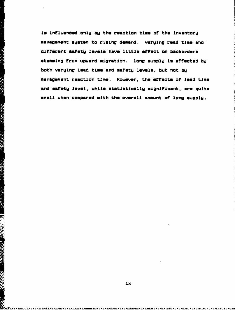
in Influenced only by the reaction time of the inventory
maiiagement sysetm to rising demand. Varying read time and-
different safety levels have little affect on backorders
stemming frum upward migration. Long supply is affected by
both varying lead time and safety levels, but not by
management reaction time. However, the effects of lead time
and safety level, while statistically significant, are quite
small when compared with the overall amount of long supply.
'I ix

A COST MODEL OF ITEM MIGRATION IN THE
AIR FORCE LOGISTICS COMMAND
CONSUMABLE ITEM INVENTORY
1. Introduction
The Air Force Logistics Command (AFLC) is responsible
For maintainLng the Air Force inventoru oF consumable items,
that is, items not repaired after theu unar out. Item
managers, with the aid of the DO-BE computerized inventoru
control sustem, track the stock level of each itmm and
request purchase oF replacement stock when needed. Stock is
purchased in quantities which minimize the overall cost of
maintaining the inventory, based on a modal oF the inventoru
system.
To avoid the time-consuming process of closelU
monitoring each oF the nearlu 600,000 items in the
consumables inventory, AFLC divides the inventorU into three
management categories. The projected dollar value oF WearlU
demand For an item determines the item's category. Items in
the high value category receive close scrutiny From the item
manager to avoid excessive backorders or costlU unnecessaru
purchases. Items in the middle category receive a moderate
degree of item manager attention. For lnw value items, item
managers depend a great deal on the DO-S2 swstem to
automaticall calcula13 stock levels and determine when to
buW more stock. Under this sWstem, an evaluation of
management practices can reveal management-related proLlems
within a specific categorW. AFLC then develops new policies
targeted for that categorW.
Item management under this sWstem becomes more
d±fficult, however, when an item's dollar value of demand
changes significantly. This causes the item to move. or
migrate, to another category. Item migration makes the
evaluation of management policies within a categorW less
straightforward. A problem with an item (for example, too
much stock or hand) maW have started when the item was in a
category other than the current one, under different
management policies. In this case, a management change in
the current category has no effect on the actual cause of
the problem. Since purchase amounts are related to demand,
item migration also leads to incorrect purchasing. A
purchase initiated when an item is in one catagorW may
arrive after the item has migrated and be coo large or too
small given the new level of demcnd.
Lt Col Palmer W. Smnith and Mr. Robert Gjmbert first
identified item migration and its effect on stock levels and
purchases a. the Defense Electronics Supply Center (DESC).
Their study covered the entire DESC inventory from 1S76 to
2

1980. A subsequent AFIT Mastern thesis bU Capt Vevin Smith
attempted to incorporate item migration into the DESC
inventorW simulation model. More recentlW, an AFIT Masters
thesis bw Capt J. D. KmnnedW has quantified item migration
within the AFLC consumables inventorW. A detailed
discussion of literature pertaining to item migration is
presented in Chapter II.
Problem Statement
Item migration complicates the task of managing the
AFLC consumables inventorW. It makes evaluation oF
management policies within management categories difficult.
Backorders result when low-demand items migrate upward. and
excess stock accrues in the low value categorW as high-
demand items migrate downward. Item migration has not been
sLccessfullU modeled, preventing anW estimate of the cost of
item migration or analwsis or new policies addressing item
migration.
Research Question
How can item migration be modeled within the context or
existing inventorU models and management practices? rhis
question gives rise to several subsidiary questions. How do
item management practices differ between management
categories? How time-dependent is the probabilitU of an
item migrating? How best can item migration be effectively
modeled? What is the dollar value of item migration in
3
terms of backorders and excess stock? What effect does
JinFormat~.on on changing demand have on the cost oF item
migration?
Research ,Oblective
It is the purpose of this investigation to develop a
simulation model o item migration within the AFLC
consumables inventory and, based on the model, estimate the
cost of item migration. This overall objective requires the
fulfillment of the following subsidiary objectives:
1. Determine the amount of migration in theconsumables inventory.
2. Create a simple model of the inventory, simulatingthe occurrence of item migration.
3. Ualidate modeled item migration.
4. Estimate the cost of item migration.
Scoose
This research is limited to item migration only within
the AFLC conrumable item inventory at the San Antonio Air
Logistius Center. Migration patterns are derived from item
migration data presented in the Kennedy thesis (Kennedy).
The simulation of the AFLC inventory is based on a
simplistic model of the AFLC consumables inventory developed
by Dizz (5:25-25). This model is modified to include item
LkL
migration. The studU does not use the large AFLC inventory
simulatior model, EDOSIM.
Overv' ew
Cheater 1I is a review of literature pertinent to item
migration. The review covers professional Journals,
technical reports, and past theses.
Chapter III presents a detailed background For the
research conducted. There is a thorough description of the
DO-62 inventory control system, including the computations
performed within the system. Ths data from the Kennedy
thesis CKennedU), which forms the basis For model
development, is covered; and lastlW, Chapter III covers the
general context in which the model will be used.
Chapter IV describes the methodology for developing the
simulation model and presents a description of the model.
Chapter IV also covers the validation of the model and
concludes with a discussion of the design of the experiment
to be performed with the model.
Chapter V presents the results of the research and
analUsis of those results.
Chapter UI contains the conclusions and implications
drawn from the analysis in Chapter V, and concludes with
recommendations for additional research.
S

II. Literature Review
Introduction
The literature review includes professional Journals
and periodicals; technical reports produced by the Air
Force, contractors, universities, and others; and past
thuses by students at the Air Force Institute of Technology.
The review covers three main areas. First, it presents
documents or studies pretaining to the AF[C consumables
inventory. Second, it discusses studies of the underlying
dynamic nature of an inventory system which gives rise to
item migration. This includes random changes in demand and
lead time (the time to receive an order of replenishment
stock oncF the order is placed) and techniques for
quantifrU..ng and dealing with these random changes. Third,
the review covers attempts to specifically analyze item
migration within inventory sustems, the approaches taken,
and results achieved.
Discussion •.•t "h Literature
AFLC Consumables Inventoru. The management of the AFLC
consumables inventory is governed by AFLC Regulation 57-6
(AFLCR S7-6). AFLCR 57-6 describes in detail the
functioning or the DO-62 computer system which automates the
management process and all management policies affecting the
inventory. Of special interest is the criterion for an item
to change management groups. An item must exhibit an annual
5

demand rate well in excess of current category
specifications for three consecutive months to enter another
category C1:12). The specific critbiia For entering each
SMSC are discussed in Chapter III, Section 1. A recent
study of the consumables inventory Found significant demand
and lead time fluctuations. This information was compared
to the way demand and lead time are modeled within AFLC'm
consumables inventory simulation, EDOSIM. EOGSIM is a
large, complex discrete event simulation of the DO-62
sWstem.. It couples the demand Forecasting techniques of DO-
62 with stochastically determined requisitions based on
actual experienced demand and an empirical distribution of
requisition size C7: Sac III, 5). EOGSIM is run on a
stratified sample of the consumables inventory. Several key
assumptions within EOQSIM concerning the stationarity of
inventory parameters may be incorrect, including the methods
for forecasting demand and lead time (8:49).
Another study of the consumables inventorW, concerned
with the impact of increasing the minimum order size,
developed a simplified model uE the inventory system (C:24-
2S). This model, created by Mr. Thomas E. Disz, aids in the
analysis of management policy changes without resorting to
the complex and possibly flawed EDOSIM model. The Disz
approach avoids the complications of stochastic demand, lead
time demand, and population sampling present in EOQSIM.
(5:25; 8:4S-50). The Diaz model employs a constant level of
7
±4j

demand over a ton Wear period. This drives a steadW series
of stock purchases to replenish the inventory. Because of
its *implicitU. the Oisz model may be run using the entire
AFLC inventory. This eliminates the need for a stratified
sample of the inventory, a potential source of error. The
modal was run several times with different minimum buy
policies. (A minimum buy is the smallest amount of stock
that can be purchased at one time, given in months of
demand.) The results provided an estimate of the cost of
different minimum buy policies C9:25,38).
Inventoru Ounamics. Inventory dynamics is a term
covering the changing nature of items within an inventory.
It includes the varying nature of demand, lead time, and
methods to analyze and compensate for this variation.
Weruino Demand. Much of the movement within an
inventory is caused by varying levels of demand. Recent
improvements in technology have contributed to the
variation. The complex technology associated with new
systems requires more complex, expensive replacement parts,
while improvements in the quality and reliability of such
parts have decreased the quantity demanded. Additionally,
many of these expensive components are modular in nature.
Modular components allow rapid replacement of failed parts,
demanding a faster response from the inventory system for
the replacement part (5:17-18). This situation results in a
S - ••r• • • i " " • . . .. .
significant number of high-cost, high-prioritU parts with
sporadic demand (5:18).
Demand within the AFLC consumables inventorW is highly
erratic. Current policies are based on the assumption that
actual demand is normallW distributed with a mean value
equal to the forecasted demand rate. But based on empirical
cata over several Wears, the actual distribution of demand
appears highlW skewed with a large number of sample demand
levels in excess of the forecasted demand rate (6:S). A
varying demand rate is a standard feature of real-world
inventorW systems, and much effort has been devoted to
expressing the variation in theormtical statistical
distributions. Such distributions allow the derivation of
explicit management policies to minimize the cost of
incorrectly predicting demand. The paWoff for such research
can be great. The Air Force consumables inventory accounts
for 6S percent of all base-level supply transactions and
seven billion dollars of yearlW Air Force requirements
(3:11). Recent changes in computing the variability of
demand at base level are expected to increase the number of
successfully filled requisitions throughout the Air Force by
14 percent C3:22). One theoretical treatment of demand
variability used a combination of the Poisson distribution
and the geometric distribution to express erratic demand.
The Poisson was used to predict the arrival of customer
requisitions, and the geometric to model the size of the

individual requisitions. The use of this distribution,
known as the stuttering Poisson, led to an empirical formula
for calculating the reorder po.Int to minimizm invaroici& cost
(19:562). :The reorder point is the level of stock nn hand
which, when reached, indicates that more stock should be
purchased.)
Varuing Land Time. Lad time variation is a major
problem for inventory managers. When an order takes longer
to arrive than expected, backorders result, and support to
inventory customers suffers. Lead time greatly affects
inventory costs. In fact, the total effect is greater than
that of demand variations over a given time period (2:158).
Aoproaches to handling lead time varu. Management policy
mau treat lead time an a constant or, as in the case of the
Air Force, use the lead time resulting from the last order
for the item in question. Additional approaches are using
the longest lead time previously occurring (to be on the
sare side) or developing a distribution of possible lead
time values using histor2:.al data (2:159-160). This last
approach was used by Bagchi, HeaUW, and Ord in developing a
distribution for demand occuring during lead time, or lead
time demand. They modeled lead time demand as a compound
distribution based on three varging elements: lead time,
number of requisitions, and the size of individual
roquisitions C2:151).
10

Safetu Level. SafetW level is a quantitU of stock
held in the inventorw. It provides a hedge against
backorders resulting from gruatur-than-expected lead time
demand. AFLC calculates sefety levels using a formula
developed bU Presutti and Trepp. The formula was derived
using the Method of Lagrange, minimizing inventorU costs
subject to a constraint on total backorders. The derivation
assumes normalU distributed lead time demand with a mean
provided bW averaging historical demand. The formula
provides the optimum amount of safetU level for a given item
based on item demand, demand variability, cost, and the cost
of a backorder (13:243,249). AFLC maW then adjust the value
used For the cost ot a backorder to remain within the budget
for safetU level expenditures (13:25O).
Parameter Estimation. Besides using a safetU
level, other techniques exist for compensatirg for
variations in demand and inaccurate management policies.
KXs parameters used in computing when and how much stock to
buU iri holding cost, ordering cost. and demand rate. These
parameters are oflen estimated, and inaccurate estimates maU
be castl.. Lowe has developed a method for estimating these
paa'ametars bW mtnrwtzing the deviation betweer the actual
average cost tncurred and the theoretical average cost given
pa-fect information abou" the distribution of demand, The
method works for both stationarU parameters (unknown but
11

fixed within a given range) and unstationary perameters
(unknown and varying within a given range) (C2:358-389).
Sig Studes. Several pmst studies have
identified and quantified item migration in different
inventory systems.
IdentifuLn= Ltm Micratia. The first research
into item migration war that of Smith and Gumbert at the
Defense Electronic Supply Center (DESC). They documented
and quantified high levels of migration between the five
DESC item management categories from March 1975 to March
1980. Their findings revealed there is an error in
evaluating the effectiveness of management category policies
based only on the observotion of items currently in the
category: items may move into a category, and the status of
such items will have nothing to do with the policies for
that category A18:t-5). A study by Kennedy has found
significant levels of migration in the AFLC consumables
inventory C11: Sac IU, 1). The analysis tracked on an item-
bU-item basis three consecutive Ueers of inventory data from
San Antonio Air Logistics Center. KennedU provides accurate
percentages of items migrating between the three AFLC
management categories from quarter to quarter
(11: Sac Ill, 3).
Modeling Item Miaration. In a follow-on effort to
Smith and Gumbert, Hobson and Kirchoff investigated the use
of a Markov chain to describe the movement of items between
12

manag'.nant categories at DISC. The transition probabilities
proved to be time-dependent and unstable using the
,management cateaories defined bU DESC (10:35,51). The use
of differart C•tsgories based on both demand value and time
in current category reduced the instability, but the
transition probabilities remained unable (10:64-66).
Further work at DISC attempted to model demand by fitting
theoretical probability distributions to demand data on
various groupings of items. The demand distributions could
then model actual demand and item migration patterns for
these groupings (16: Sac I1, 5). However, *Simulation
results were very dependent on the item characteristics used
to define the groupings" (16: Sac U, 31). The item
migration patterns from the model did not match observed
item migration patterns CIS: Sac U1, 3).
Proposed. Policu Chanoges Addressina Item MiRration.
Although Markov chains failed to modal DESC item migration,
Hobson and Kirchoff used DESC migration patterns to develop
a proposed policy for buying replenishment stock in medium
and high value categories. A comparison of the time an item
had been in a category and the percentage of time such an
item would migrate to a lower category showed a linear
relationship C10:.S-71). The proposed policy used this
relationship to decrease the size of replenishment order
based on the time in category. For medium value items, this
involved buying about 60 percent of a normal order for an
13
MK.

item in the categoru for only one quarter. This percentage
Increased linearlU with time until a full order was
recommended for items with mure than 1e quarters in a
category. High value order size varied from three months
worth of demand for items ii. the catwgorW fMr ucr.lWu n
quarter, climbing to a 12 month maximum order size
(specified bU regulation) when the item exceeded eO quarters
in the category C10:71-7e).

8EL Manaenmant
fth Economi Qrder gumntitu &UU~tMM9 Ginnuta1mnSuals. DO-Be is a computerized data management
sUstem designed to gather data, compute requirements, and
provide the information necessary for intelligent management
of the non-rmroverable items in the AFLC inventory. The
system has two computation processes. One computea and
identifies procurement actions required for support of 0OD
missions. This is done on an exception basis, when items
fall outside specific parameters within DO-Be (1:13). The
other process projects funding requirements for the
procurement of necessary stock. This research effort is
concerned with the former, the item management function of
DO-Ba.
The primary function of 0O-68 for item management is
the computation of stock levels and projected requirements.
Requirements are forecasted based on past demands. "The
sUstem runs four times each month using the most current
asset...and demand date..." C1:13). DO-62 items are managed
"by exception". Computations and updates to stock levels
and demands are performed automatically, and the item
manager is notified only when the asset position for an item
violates specified parameters (1:13). For example, when the
15

stock level for an item falls below a certain level, the
system generates a notice to purchase more stock.
DO-62 13 structured so that management intensity for an
item depends on the dollar value of demand for that item.
High demand value items are given the closest scrutiny to
ensure effective, cost-efficient management. To this end,
items are categorized by their annual dollar value of demand
into Supply Management Groupings, denoted by a SupplU
Management Grouping Code (SMGC) (1:12). The item data used
in this study are from June 1581 to March 1598. At that
time AFLC used four SMGCs. In December 1S81 AFLC reduced
the number of SMGCs to three, but since all data are based
on four SMGCs, the pre-December 1i84 SMGCs are used (11: Sac
II, 3). The four groupings are:
SMC X. These are the low value items, with a
UearliU demand value of SO - $500. Items in this SMGC
receive a low level of management intensity. Item data are
raviewed occasionally for accuracy. If an item in this SMSC
has an annual demand rate of $2600 or more for 3 consecutivn
months, the item is reassigned to another SMSC.
SMGC T. These are the medium value items, with a
WearlU demand value of 5S00.01 - 5S,000. Items in this SMGC
receive a moderate level of management intensity. Item data
are reviewed regularly for accuracy, especiallU when the
system indicates that more stock should be purchased. If an
item in this SMGC has an annual demand rate of less than
16

'00.01 or more then 55,100 for three consecutive months, the
item is reassigned to another SMGC.
SMC P. These are the high value items, with a
yearly demand value of 55000.01 - $50,000. Items in this
SMGC receive a high level of management intensity. Item
data are reviewed often for accuracy, and is closely
reviewed when the system indicates that more stock should be
purchased. If an item in this SMSC has an annual demand
rate of less than 4900.01 or more than 350,000 for three
consecutive months, the item is reassigned to another SMGC.
SMlC M. These are the very high value items, with
a WearlU demand velue of over 550,000. Items in this
"category receive a very high degree of managemmnt intensity.
Item data are reviewed constantlW, and all data involved in
the computation of a purchase request are scrutinized to
ensure no unnecessary stock is purchased. Large
requisitions for stock are also double-checked to make sure
the user has a legitimate need for a large quantity of such
high-value assets. If the annual demand for such en item
falls below *9,000.01 for 3 consecutive months, the item is
reassigned to a lower category (1:12,22).
Hioh intensitu. High intensity management may be
&pecified for an item in any SMGC when that item has great
impa.7t on supply availability (fill rate) or when the ALC
responsible believes that intensified management will
significantly improve support. Items so specified receive
17

the highest degree of management intensity. All input data
are screened extremely carefully, and all management actions
are subject to close scrutiny for accuracy, completeness,
and timeliness (1:12-13,22-23).
Functions of DO-52. This section covers the main areas
of item information calculated and/or maintained bW DO-62.
This information allows DO-62 to accuratesi] track the status
of items within the system, maintain a history of the demand
for the item, and forecast future demand for the item. DO-
62 maintains information on assets, past demand, end
projected requirements; calculates vLrious stock levels; and
computes the economic order quantity for purchases of
replenishment stock.
Assets. Assets are the stock available within the
system to meet the demands of item users. Assets fall into
several categories. Item manager controlled assets are
stored in depot supply warehouses. The issue of these items
is directed by the item manager. Depot supply assets are
issued by the item manager to the depot to cover the
required depot supply level. These assets are issued by the
depot supply clerk. In-transit assets are stock being moved
from one depot to another. Due-in assets are stock which
has been purchased but has not Wet been received, as well as
stock arriving from reclamation or as support from other
services (1:20,21). Unservicable assets are unservicable,
repairable items which are expected to be repaired to
18
M?%AnA
serviceable condition. The number of unservicable items is
multiplied by a condemnation factor to determine how manw
are expected to be returned to service (1:21). Since DO-62
items are considered non-recoverable, the condemnation
Factor is usually 1.0, leaving zero unservicable assets for
use in the total asset computation.
Assets used in computation are the total of the above
asset categories. This total is used in all calculations in
DO-52 requiring total available assets for an item (1:20).
Demand historu. As stated above, 00-62 uses past
demand data to project requirements for support. The sastem
maintains a past history of the current quarter and last two
Wears (eight quarters) demand data for each item. Demand
data include demand history bw quarter, stock returned
unused, the demand level used in DO-62 computations, and
requisition frequency.
Demand history bw quarter is the sum of the quantities
on all requisitions received during the quarter unless the
requisition was cancelled bw the item manager. These are
demands bw and users only, not shipments to depot supply or
other storage sites. Demand history includes total sales,
one-time demands, and transfers to base-level supply. Total
sales is stock issued bw both the item manager and depot
supply (1:13-14). Besides Air Force maintenance functions,
end users include overhaul and repair contractors end other
services and DOD agencies. One-time only demands are

generated bU activities such as initial activation oF a
sUstem or a one-time exercise. These are recorded as non-
recurring demands and are considered in projecting demand
for low demand value items. Transfers to base-level supp1U
are free issue, so reimbursement occurs when the sale is
made at base supplU (1:13).
Serviceable returns are stock that was returned to the
depot in suitable ccodition for re-issue. Returns are
identified to the original stock issue.
DO-62 computes a level of demand for use in DO-62
computations. Demands used in computation are calculated
differentlU for different SMGCs. Within SMGC X and T,
demands used in computation equal the total sales plus non-
recurring demands plus transfer demands. Within SMSC P and
M, demands used in computation equal the total sales plus
transfer demands minus serviceable returns (1:78).
Requisition frequencU is a quarterlU count of the
number of requisitions received. Non-recurring requisitions
are not counted (1:14).
Requirements. Requirements are projected demands
for items. D0-62 tracks several areas of requirements data
-- monthlU demand rate, program demand rate, quantitative
requirements, depot level maintenance requirements, and
several requirements factors.
McnthlU demand rate is the expected rate of monthlW
demand determined from the demand historU discussed earlier.
20
LI

It is* computed bgj taking the average of the quarterly demand
over the last eight quarters. This is a moving average,
always based on the current quarter and the eight quarters
just preceding. There is an option to us. only the four
previous quarters when the item manager believe. this will
give a more accurate projection of demanri C1:13-14i,78).
Quantitative requirements are known additional
requirements for the next three Wears, over and above the
projected demand indicated by item history. Quantitative
requirements are added to the program demand rats for the
quarter in which they will occur to project the total
support required in that quarter (1:16).
Depot level maintenance requirements, as the name
implies, are parts requirements for depot level maintenance.
They are computed separately. The schedule for much
maintenance is known with certainty, arnd therefore, so is
the parts requirement. This requirement is also added to
the program demand rate for total demand projections (1:16).
Requirements factors are used in projecting
requirements. TheW are either supplied by AFLC invenltory
management or computed within the DO-62 sustem. The primary
requirements factors are the peacetime program ratio CPPR)
and lead time. The PPR is a factor used to adjust the
monthly demand rate to reflect upcoming changes in the rate
of use For the supported system. The program demand rate is
the monthly demand rate multiplied by the PPR (1:78). For
21
example, a known increase in flying hours for a particular
aircraft will result in a PPR greater than one for some
components of that aircraft, to reflect the increased
consumption of parts. For items with no usage fluctuations
from increases in system operation, the PPR equals one.
Lead time is the number of days between the time DO-B2
outputs a notice to buy stock and the time when tan percent
of the normal deliveries of that order arrive. Lead time
has two components, administrative lead time and production
lead time. Administrative lead time is the amount of time
that elapses from the output of the buy notice to the
letting of a contract for the procurement of the required
stock. It consists of both the time it takes for the
Directorate of Materiel Management (MM) to prepare a
purchase request, and for the Directorate of Contracting and
Manufacturing (PM) to process the purchase request and award
the contract or purchase order. The MM time is a maximum of
30 days for SMGC X items, 2l days for T and P items, 16 days
for M items, and 14 days for high intensiity management
items (1:14). The PM time is projected from the previous
procurement action for that item. If the previous
procurement is not representative of a normal buy, the item
manager may substitute a more realistic PM time C1:15).
Production lead time is the amount of time it takes the
contractor to produce the required stock, beginning with the
letting of the contract. The time of stock arrival is the
22
time when ten percent of the total normal deliveries of the
purchase have arrived. Normal deliveries do not include~
special "rush orders" arriving ahead of the bulk of the
purchase. Production lead time is projected by using the
time required during the previous purchase for the item. If
that purchase was not representative of a normal purchase of
that item, the item manager may substitute a more realistic
production lead time (1:15).
Computed Levels. Computed levels are the internal
control parameters on DO-62 assets. When asset position
violates a level, a notice of the occurrence is printed for
the item manager. The two most important levels are the
reorder level and the safety level. The amount of stock due
out, leand time demand, and the amount of funded war reserve
materiel all influence the level computations.
The reorder level (ROL) is that level of stock on hand
which, when reached, indicates that more stock should be
ordered. It is equal to lead time demand plus due-outs plus
safety level plus depot supply level plus funded war reserve
materiel. Each of these components is discussed below
Lead time demand is the projected demand for the item
during lead time. It is the sum of the F'ollowing two demand
projections: (1) the program demand rate computed from
historical data multiplied by the lead time and (2) the
quantitative requirements projected during lead time (1:79).
44 23

Due-outs are stock alreadu committed to issue. Due-
outs are added to the ROL since they cannot be used to meet
demands during lead time (1:15). Depot supply level is the
amount of supply required at depot level for each of the
five ALCa. Funded war reserve material is all funded
requirements for war reserve materiel on hand, on order, or
to be bought (1:19).
Safety level is a variable quantity required to help
support peak periods of demand and minimize shortages. The
safety level factor K is the number of standard deviations
worth of lead time demand (denoted as 0) to allow as a
safety level on a particular item. The computation of K and
0 are explained in the following paragraphs.
First compute the mean absolute deviation of demand
CMAD). MAD is the average over the item history of the
difference between each quarter's actual not recurring
demands and the quarter average projected by historical
data. The formula for the absolute deviation (AD) for each
quarter is:
AD - I0emands - (3 ' monthly demand rate)I
The formula for MAD is:
MAD - sum of ADs for all quarters in computationnumber of quarters in computation
24
MAD is converted to the standard deviation of lead time
demand CS) by the equation:
8 - PPR 0 .S9e*MAD * (.82375 + .4252S5leadtime)-*.85
where .82375 and .4252S express MAD over lead timeand recognize that a particular month's demands areinfluenced by previous months' demands, and .55converts the quarterly MAD to a monthly MAD (1:00).
With these computations complete, the formula for K is:
K - -. 70701n Vf' GacS ze c 1 -exp c-7- 375-5>
where
a - holding cost factorc - unit costa - economic order quantity (discussed later)
- implied shortage factor2 - 31 square root of average requisition size8 - standard deviation of sad time demand.
The value of K must be greater than or equal to zero;
so, if this equation returns a negative value, K is set
equal to zero. The safety level equals K*8. The average
requisition size is obtained by dividing the actual demand
for the item over the item historw bw the number of
requisitions C1:80). The economic order quantity is
discussed in the next paragraph.
Purchase of stock. DO-62 initiates a notice For
the item manager to prepare a purchase request when the
assets on hand fall below the reorder level. DO-S2 also
computes the Economic Order Quantity (EOQ) (1:19,22). This
25
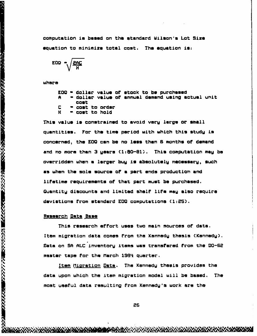
computation is based on the standard Wilson's Lot Size
equation to minimize total cost. The equation is:
EO - AC
where
EDO - dollar value of stock to be purchasedA - dollar value of annual demand using actual unit
costC - cost to orderH - cost to hold
This value is constrained to avoid very large or small
quantities. For the time period with which this study is
concerned, the EGO can be no less than B months of demand
and no more than 3 Wears (1:80-81). This computation maw be
overridden when a larger buy is absolutely necessary, such
as when the sole source of a part ends production and
lifetime requirements of that part must be purchased.
Ouantitw discounts and limited shelf life maw also require
deviations from standard EGO computations (1:25).
Research Data Base
This research effort uses two main sources of data.
Item migration data comes from the Kennedw thesis (Kennedy).
Data on SA ALC inventory items was transferud from the DO-62
master tape for the March 1984 quarter,
Item Micration Data. The Kennedy thesis provides the
data upon which the item migration model will be based. The
most useful data resulting from Kennedy's work are the
26
- -
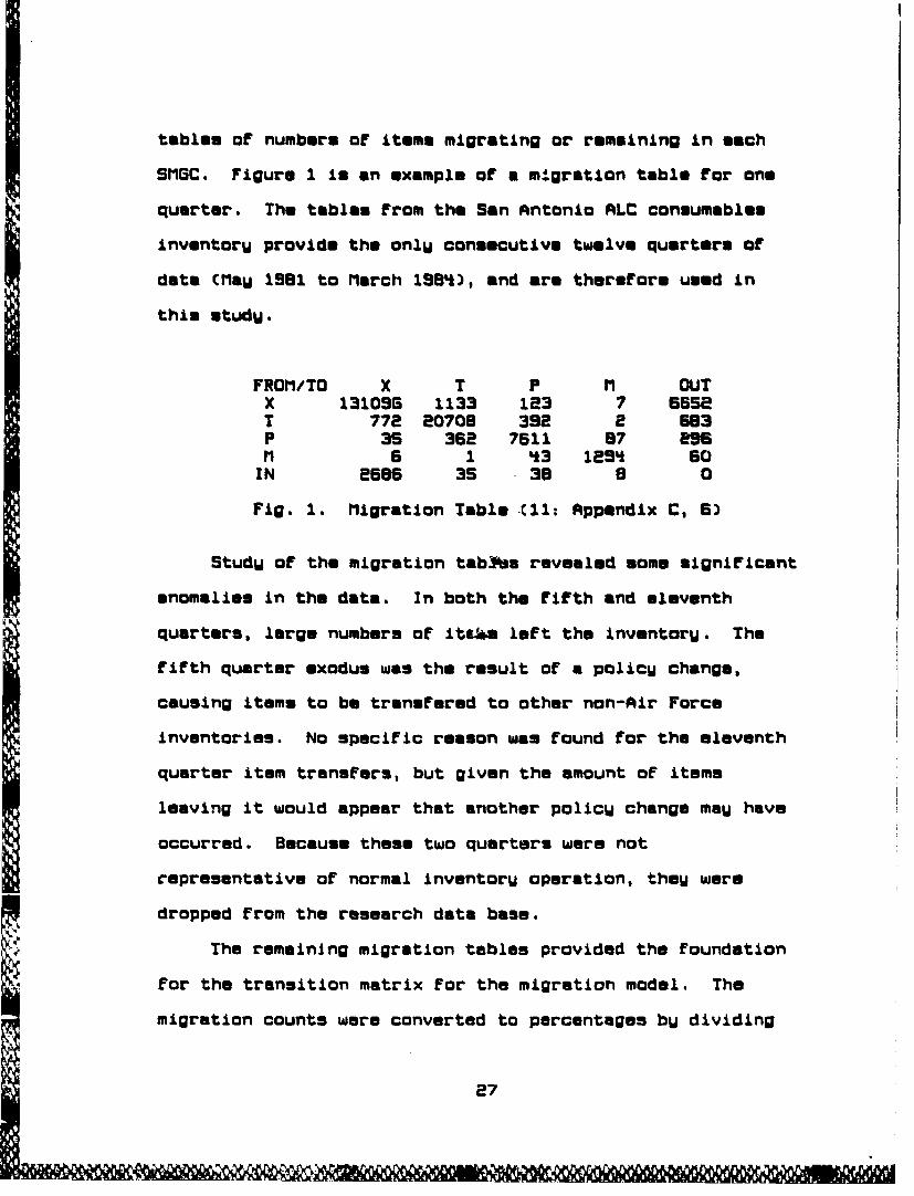
tables of numbers of items migrating or remaining in each
SMSC. Figure 1 is an example of a migration table for one
quarter. The tables from the San Antonio ALC consumables
inventorU provide the only consecutive twelve quarters of
data (Maw 1981 to March 9S84), and arm therefore used in
this study.
FROM/TO X T P M OUTX 131096 1133 123 7 665eT 772 20708 392 a 583P 35 352 7511 87 e96M 6 1 43 129* 50
IN 2586 35 38 8 0
Fig. 1. Migration Table Cl1: Appendix C, 6)
StudU of the migration tab-s revealed some significant
anomalies in the data. In both the fifth and eleventh
quarters, large numbers of itL"i left the inventory. The
fifth quarter exodus was the result of a policy change,
causing items to be transfered to other non-Air Force
inventories. No specific reason was found for the eleventh
quarter item transfers, but given the amount of items
leaving it would appear that another policy change mau have
occurred. Because these two quarters were not
representative of normal inventory operation, they were
dropped from the research data bass.
The remaining migration tables provided the foundation
for the transition matrix for the migration model. The
migration counts were converted to percentages bU dividing
27

each row entry by the sum of the entries in the row. Each
migration percentage was averaged over all quarters. This
resulted in the transition matrix shown in Figure e.
FROM/TO X T P M OUTX .544888 .019E88 .001377 .000157 .00L656T .Oe'5S3 .899571 .03L441O .000850 .0e50*eP .007961 .043185 .907705 .01769k .023858MI .004731 .001040 .041668 .SeRS99 .0eS86e
IN .503474 .063613 .086530 .006383 0.0
Fig. e. Migration Transition Matrix
Kennedy also provided data on the relationship of
migration to the amount of time an item has boon in a SMGC.
All items in each SMIC at the start of the twelve quarters
of data were tracked until they left the SMOC. This showed
the draw-down of items within the SMOC over time. Items at
DESC had been found to be less likely to migrate the longer
they remained in a category (18:10); KennedU sought to find
out if the same was true at AFLC. If it was, one would see
a decreasing percentage of items leaving the initial group
in the SMSC from quarter to quarter. Analysis of the draw-
down of the initial stock of items in each SMOC does not
support this premise. The fraction of items leaving each
quarter shows no detectable pattern over the twelve quarter
period for anW of the SMGCs. For this reason no attempt was
made to incorporate any time-related migration data in the
model.
Inventoru Data. Item data was gleaned from the 00-62
master tape. The tape was ruad onto the AFIT UAX 11/780 CSC
28

computer system as an ASCII text file. A FORTRAN program
extracted the following fields:
1. Price: the actual unit price.
e. Total assets: the sum of assets used in
computation, as discussd in Section 111-1.
3. Peacetime program ratio.
4. Program monthly demsand rate.
S. Lead time.
6. Mean absolute deviation.
7. Average requisition size.
The AFLC data presented the same problem encountered by
Disz: some numerical fields carried the sign as an
overstrike on the last character in the field (S:36). A
modification of Diazls FORTRAN subroutine to translate the
ovarstrikes, incorporated in the program to extract the
data, alleviated this problem CS:74-75).
The data described above formed records for each of the
nearly 10,000 items in the SA ALC inventory. This master
file was then sorted into separate files for each SMeC.
AdditionallU, SMGC X was divided into two files: one for
items with zero demand and one for items with non-zero
demand. This sorting provides for later statistical
analUsis of item data within each SMOC and for zero demand
items.
2S

Model Context
Any model of item migration within the AFLC consumables
inventory should start with a model of the inventory itself,
including the management procedures and policies used by
AFLC. In this way item migration may be modeled within the
context of AFLC inventory management, and the influence of
that management on item migration may be explored. Without
a solid model of the AFLC inventory as a foundation, a
migration model oan provide no meaningful insights into AFLC
item migration.
Item migration is nothing more than a change in the
dollar value of demand for an item that is large enough to
propel that item into a different SMGC. The limits of the
SMOC are a threshold over which demand changes must rise to
cause the item to migrate. A model of item migration should
show the effect of demand changes above this threshold. The
effects of migration are most visible in terms of backorders
and excess stock on hand, so the model should provide these
performance indicators.
Information on demand changes also may contribute to
the effects of migration. The model should allow for
evaluating the effect of the speed with which the inventory
management system recognizes the new level of demand for a
migrating item. The DO-62 system currently has a one
quarter lag between demand change and item migration. The
30
affect of instantly recognizing the demand change and moving
the item to the now SMGC may be considerable.
There are other factors which may contribute to or
mitigate the effects of migration. Lead time often
increases as the dollar value of demand increase, since
larger orders take longer to process and fill. Lead time
changes also contribute to backorders. The model should
provide for a comparison of migration effects with lead time
hold constant and with changing lead time. Another factor
influencing backorders is the implied shortage factor. The
implited shortage~ factor is determined from the amount of
funds available for safety level stock. The less safety
level funding available, the smaller the implied shortage
factor, and the lower the safety level. Lower safety levels
allow a greater potential for backorders. The model should
allow for different values of the implied shortage factor to
determine the effect of safety level on migration-induced
backorders..
31
IV. Methodoloau
Model Development
This research effort centers around the use of the Disz
inventorw simulation model described in Chapter II. To
effectivelU model item migration, the Disz model requires
extensive modification. Manw assumptions and simplications
concerning the DO-62 swstem are also necessarw to keap model
complexitU within manageable limits. First, keU assumptions
and simplifications are incorporated in the model. Then,
specific modifications to the Disz model allow the it to
model migration within the context of the AFLC consumables
inventorw.
Assumptions and Simplifications. The DO-62 swstem,
discussed in Section II, is a verU complex inventorg
manager3nt sWstem. Without significant simplifications, a
model nf DO-S2 would be so large and cumbersomv that
validation and analwsis of results would be difficult if not
impossible. Assumptions about the nature of items within
the inventorW are also necessarU. Within the simulation
model, items need to be created to enter the inventorU. The
parameters associated with these items should conform as
much as possible to those of real items, and this requires
assumptions for a "twpical" item entering the inventorW.
The following paragraphs discuss the assumptions and
simplifications underlwing the item migration model.
32

The greatest simplification of the model is the use of
a constant, or "straight line", demand for items in the
inventorU. The Disz model also used this simplification.
Items will migrate between quarters, so the demand during
any one quarter will be at a constant rate, with the
possibility of an instant change to a different constant
rate For the next quarter if migration occurs. If the item
does not migrate, demand continues at the same coistant
rate. The substitution of constant demand for random demand
allows the model to eliminate backorders caused by small
demand fluctuations. The backorders generated will be the
result of item migration only. Additionally, constant
demand greatly reduces the complexity and required
computational effort of the model.
QuarterlW migration is modeled based on the assumption
of a stationary Markov process. The cumulative transition
matrix discussed in Chapter III provides the prohability of
migration for items in each SMUC. This is similar to the
approach attempted by Hobson und Kirchoff; however, the same
stationarity criteria is not applied. The model centers on
approximating AFLC migration patterns to a reasonable level
to allow valid experimentation within the model.
Another important assumption is that all items in an
SMOC have an equal chance or migrating. This disregards the
possibility of items near the boundary of the SMOC having a
greater likelihood than other items of migrating the short
3-
|N
distance to the adjacent category. Support for this
assumption comes from the significant amount of large demand
changes within the D0-62 sustam. According to an AFLC
study, during a twelve quarter period, 38.5 percent of the
items in the SA ALC consumables inventory experienced a
demand fluctuation of from 50 percent to over 5900 percent.
Item migration appears to involve considerable changes in
demand (4:12). Additional support for this assumption comes
from Dr. Palmer W. Smith. Quoting his work at DESC, Dr.
Smith points out that over a nine quarter period at DESC,
less than 0.10 percent of the items in the 1 million item
DESC inventory moved back and forth between adjacent
categories every quarter, and only 0.20 percent moved back
and forth between adjacent categories every two quarters.
The lack of back and forth movement also shows that item
migration is not a transient change in demand. Items in
general do not jump back and forth across a categoru
boundary (17).
To further simplify the model, certain item parameters
are held constant. These parameters are mean absolute
deviation of demand (MAD), average requisition size (ARS),
and peacetime program ratio (PPR). Once an item is read in,
the values of these parameters remain the same as long as
the item remains in the simulation. As items are created to
enter the inventorW, the simulation assigns point estimates
of these parameters based on the average values of the
34
7 '..VU

parameters for the SMGC the created item is entering. Any
missing parameters are assigned values in the same manner.
Item prices are also hold constant. This assumption is
supported by a recent AFLC study showing that item migration
is primarily the result of changes in demand, as opposed to
changes in price (4*:9,11). Prices for new items entering
the inventorW are based on the empirical distribution of
pric~es in the SMGC the item 'is entering.
Lead time is an important parameter within the
simulation. Lead time often changes as demand changes,
since items at different levels of demand fall under
different procurement rules. Procuremnent rules affect the
amount of administrative lead time, and therefore aFaect
total lead time. Item migration involves a significant
change in demand, so item migration and changes in lead time
may often coincide. The simulation provides two options for
dealing with lead time. The first is to hold an item's lead
time constant throughout the simulation. The second option
changes the lead time when an item migrates. The new lead
time value is a point estimate based on the average lead
time For the SMGC the item is entering. Under either
option, created items receive the average lead time for
their initial SaIGC.
As previously stated, the level of demand for an item
changes only when an item migrates. To assign a now dollar
value of demand to a migrated item, a distribution of dollar
3S
demand values for the new SMGC is needed. A histogram of
dollar demand for each SMOC shows a strong resemblance to
the exponential distribution. Unfortunately, goodness-of-
fit tests on random samples from each SMOC failed for both
the exponential and log-normal distributions. Because of
the strong resemblance to the exponential, however, dollar
demand values were assumed to be exponentiallu distributed.
The lower limit of the SMGC provides the location parameter
for the exponential distribution, and the mean is set equal
to the average dollar demand value for the SMGC minus the
lower limit of the SMSC. Values generated in excess of the
upper limit of the SMOC are discarded, and another value is
generated.
To summarize the basic assumptions and simplifications
of tha model, most item parameters are held constant, and
new items receive parameter values created
deterministically. The demand rate during any quarter is
constant. Demand only changes when an items migrates, and
then the change is a discrete Jump to a different constant
demand rate. OnlU two parameter values are generated
stochastically. The SMGC of an item for the next quarter in
the simulation comes from a random draw to sample the
cumulative transition matrix. This determines item
migration. If the item migrates, the second stochasticllU
generated value is the dollar value of demand within the new
SMSC.
36
Modifications to the Diaz Model. The Disz modal
required several significant modifications to effectively
model the dynamic inventory scenario associated with item
migration. The original Disz modal maintains constant,
unchanging demand for the length of the simulation. This
means no backorders and no item migration can occur. No
differentiation is made between stock purchase and arrival;
stock arrives instantly at the end of each procurement
cycle. There is no movement of items in and out of the
inventory. To alleviate these shortcomings, several new
model components were created.
The first modification is a means to generate quarterly
item migratiun. At the start of each quarter, the model
co~npares a standard uniform random number to the row of the
transition matrix corresponding to the current SMGC of the
item. The range of values within which the random number
falls determines the SMGC for the next quarter. If the item
migr as, the new level of demand comes from the exponential
distribution of demand for the new SMGC, obtained from the
inverse transform of the exponential cumulative density
Function acting upon a standard uniform random number.
The importance of lead time, occurring between stock
order -nd ival, requires the model to track the days
within each quarter. When the reorder level is breached,
the model places the order by scheduling the order to arrive
at the end n he lead time. Lead time is converted from
37
Zm~ii

days to quarters and days, and is added to the current
quarter and day to determine the time of arrival. Each day
during the simulation the current quarter and day are
chocked to sea if an order is to arrive that day. The
average number of days in a quarter is 91.25. To allow the
computer n~rogram of the model to loop on integer values, the
model uses 51 days per quarter. Real days are converted to
these slightlW longer days by multiplying by 91/51.2S.
The length of lead time For some items exceeds the
length of time the economic order quantity of stock for
those items will last. To deal with this possibility, the
reorder level is compared to the assets on hand plus the
assets on order. Lead time becomes a "pipeline" oF stock on
order scheduled to arrive when on hand assets reach the
safety level. Each order has its own arrival date, and each
daW of the simulation all inbound orders are checked to see
if an order arrives that day. The model provides for
several orders to be inbound at anw given time.
Another change to the model involves generating inbound
orders of stock when an item enters the simulation. At the
beginning oF a simulation run, many items in the inventory
will have assets below the reorder level and orders due to
arrive in the future. The model is modified to determine
the dates of order arrival bW calculating the times from the
start oF the simulation through one lead time when, under
the current demand rate, the asset level Falls to the safetW

level. These times are the scheduled arrivals of an
economic order quantity of stock. The inbound orders raise
the level of assets on hand plus assets on order above the
reorder level, and the normal order-placing mechanism of the
model takes over. If the asset position is at or below the
safety level at the start of the simulation, a full order
plus anw safety level replenishment is added before the
simulation begins.
To simulate items entering the inventorU, the model
must create now items. New items are generated after the
simulation has run on the items present in the inventory at
the start or the simulation. The number of items generated
during each quarter is set equal to the number of items that
left the inventorw during that quarter to maiT,,ain a
constant number of items in the inventorU. The fifth row of
the transition matrix determines the proportion of new items
going into each SMGC, and the demand is calculated using the
exponential distribution discussed above.
The unit price of the new item comes from the empirical
price distribution for the specific SMSC. For the items
entering a given SMGC in a given quarter, the first ten
percent receive the average of the lowest ten percent of the
prices of items in the SMGC. The next ten percent entering
receive the average price of the next lowest ten percent of
prices in the SMGC, and so on (see Figure 3).
39
Q
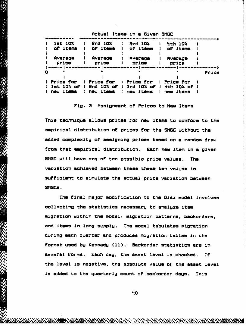
Actual Items in a Given SMOC
I lot 10% 1 End 10% I 3rd 10% 1 Ith 10% II of items I of items I of items I of items II I I I II Average I Average I Average I Average I
price I price I price I price IS I ---------- I-- ---------- I-- -------I -------------
0 .. a.aPriceI l I I
I Price for I Price for I Price for I Price for II lst 10% or I End 10% of 1 3rd 10% or I Ith i0% of II new items I new items I new items I now items I
Fig. 3 Assignment of Prices to New Items
This technique allows prices for new items to conform to the
empirical distribution of prices for the SMGC without the
added complexitU of assigning prices based on a random draw
from that empirical distribution. Each new item in a given
SMGC will have one of ten possible price values. The
variation achieved between these these ten values is
sufficient to simulate the actual price variation between
SMGCs.
The final major modification to the Disz model involves
collecting the statistics necessaru to analUze item
migration within the model: migration patterns, backorders,
and items in long supplw. The model tabulates migration
during each quarter and produces migration tables in the
format used bW KennedW (11). Backordar statistics are in
several forms. Each daU, the asset level is checked. If
the level is negative, the absolute value of the asset level
is added to the quarterlW count of backorder dams. This
40

figure is also multiplied bU the item price to track the
quarterlU dollar-weighted backorder dr.Us. Backorders arm
also counted when replenishment stock arrives, since this is
the point when maximum backorders exist. The model tracks
the total maximum backorders and dollar-weighted maximum
backorders occurring in each quarter. FinallU, at the end
of s,.;i quarter in the simulation, items with assets in
excess of the Approved Force Aquisition Objective (AFAO)
count as items in nlong supplU." The AFAO is defined for
SMGC X as the reorder level plus one economic order quantity
plus stock for one Usar of demand. The AFRO for SMGCs T, P,
and M is the reorder level plus the greater of either the
economic order quantity or stock for two Uears of demand
C1:81). The number of items in long supply and the dollar
value of the excess stock are collected for each quarter.
Model •Descriation
The inventorU simulation model developed through this
research effort is called MIGSIM. MISIM is programmed in
FORTRAN 77 and currentlU runs on the VAX 11/760 Classroom
Support Computer (CSC) sUstem at the Air Force Institute of
TechnologU. As is tUpical of manu computer simulations,
MIISIM consists of a main program driving several
subroutines which carrU out most of the important aspects of
the inventory simulation. MIGSIM is compact enough to run
using the entire consumables inventory of the San Antonio
ALC, about 1*0,000 items; however, because of the need for
Li1

multiple runs and hmavy utilization of computer resources,
MIOSIM currently runs on a ten percent sample of the San
Antonio ALC inventory. Ten percent of the items from each
SMOC, selected at random, comprise the sample. SMOC X,
because of the large number of zero demand items, was split
into two groups: zero demand and non-zero demand items. Ten
percent of each of those two groups was included in the
sample. During the simulation, Items have an opportunitu to
migrate to a different SMSC each quarter.
MISSIM mau be configured to run in three item migration
modes. The first is with no item migration, similar to the
original Disz model. The second is with instant recognition
of item migration. When demand changes and an item
migrates, all levels are recomputed immediatelU with the new
item parameters. The third mode includes a one quarter lag
in the recognicionn bU the inventoru management sUstem of a
migration and accompanuing demand change. For one quarter,
the item is managed according to the old level of demand
while stock on hand is actuallu reduced at the new demand
level in the new SMGC. This third mode is equivalen: to the
manner in which AFLC currently treats item migration; an
item must exhibit the new demand level for three months Cone
quarter) before the item is moved to the new SMGC.
The MISSIM source code listing, thoroughly commented,
is contained in Appendix A. For information on the FORTRAN
formulation of specific aspects of the simulation model,
'*2

refer to Appendix A. The following paragraphs present a
general discussion of the functions performed by the main
program, called MAIN, and each subroutine.
MAIN. MAIN is the central component of MIGSIM. MAIN
reads in item date from an external file for each item in
the inventory at the start of the simulation. The
cumulative transition matrix and table of prices for items
entering the inventory are read into arraus. MAIN contains
the initial values for the random number generator seeds
associated with the two stochastic events in the simulation:
migration and the resulting new demand level. Finally, MAIN
initializes all statistics collection variables to zero
before the simulation starts and writes to a file all output
statistics at the end of the simulation.
Subroutine BUYDUE. BUYDUE is the first subroutine to
process an inventory item when the item starts the
simulation. BUYDUE calls subroutine LEVEL, discussed below,
to obtain the reorder level, safetu level, and the EOO; and
compares the currant asset level to the reorder level. If
assets are below the reorder level, BUYDUE establishes a
timm period equal to lead time, beginning at the item's
entru into the simulation. BUYDUE then schedules the
necessary EDO orders of replenishment stock to arrive at the
precise times during that time period when, undar the
current demand rate, the asset level will reach the safety
level. For items with long lead times and small EO0s, more
43
!.I *'I

than one inbound order mau be needed. The amount of stock
and time of arrival for each order is stored in an array to
be added to stock on hand at the correct time in the
simulation. This process accounts for the arrival of orders
placed before the simulation begins. The inbound orders
raise the asset position above the reorder leve~l before the
start of simulated demand.
Subroutine CYCLE. CYCLE is the heart of the actual
inventory management simulated in MIGSIM. CYCLE subjects
inventory items to up to twelve quarters of demand and
provides a quarterly opportunity for item migration. CYCLE
carries out the main functions of the 00-52 system -- it
calculates levels, orders replenishment stock, and schedules
stock arrival. Additionally, CYCLE collects quarterly
statistics on backorders, dollars spent on stock, items in
long supply, an~d the actual demand experienced by the
inventory.
To model item migration, CYCLE uses the stand~ard
uniform random number generator present in FORTRAN on the
CSC. Each quarter, a random number is compared to the row
of the cumulative transition matrix corresponding to the
item's current SMGC. CYCLE determines the smallest column
value greater than or equal to the rendom number, and that
column corresponds to the item's SMGC for the next quarter.
If the next quarter's SMGC is different From that of ths
previous quarter (the item has migrated), then CYCLE calls
44~

the subroutine GETDEM, discussed below, to get the new
demand level. CYCLE then recalculates levels, either
:immediately or after a one quarter lag, depending on the
migration mode.
Subroutine GETDEM. GETDEM generates the now dollar
value )f demand for items migrating to SMGCs. As described
in Section IU.1, the distribution of demand is modeled as
exponential. GETDEM uses the resident standard uniform
random number generator to drive the inverse transform of
tee exponential cumulative density function for the new
demand value. This process is modified somewhat for items
entering SMGC X. Because of the extremely large number of
zero demand items in SMGC X, a simple Monte Carlo draw first
determines whether the item will have a zero or non-zero
demand. IF the demand is to be non-zero, CYCLE generates
another random number and uses the exponential distribution
to determine the exact demand.
Subroutine ADDNEW. Item migration includes items
leaving the inventory and new items entering the inventory.
ADDNEW creates the new items entering the inventory and
assigns parameters to those items. The total number of
iteaia to enter the inventory each quarter is set equal to
the number that have left the inventory during that quarter.
ADDNEW is called after the simulation has run for all items
in the original inventory, and ADDNEW proceeds by quarter
from the first quarter to the twelfth. So when ADDNEW
45

II
prepares to generate nfw items for a given quarter, the
number of items (both original and previously created bU
ADDNEW) that have left the inventory during that quarter is
known precisely. In this manner the number of items in the
inventory remains constant, eliminating anW confounding
effects caused by fluctuations in inventory size. This is
also consistent with the assumption of a stationary Markov
process.
The proportion of new items entering each SMGC is
provided by the transition probabilities For the "IN"
category of the Markov process. ADDNEW generates the
required number of new items for each SMGC sequentially,
first the SMGC X items, then the SMGC T items, and so on.
Subroutine GETDEM is called to determine the dollar value of
demand based on the SMGC. The technique for assigning
parametric values to a new item is also based on the SMGC
and was covered in Section IV.1. 7 or items with non-zero
demand, ADDNEW calls BUYDUE to set the initial asset level
and schedule inbound orders. Items with no demand receive
assets on hand equal to fifteen and no inbound orders.
(Fifteen is the average asset level for zero demand items in
the actual inventory.)
Once the new item has the necessary assets and inbound
orders, ADDNEW calls CYCLE, and the simulation begins at the
quarter specified by ADDNEW. To insure that the item
experiences one quarter of demand in the SMGC specified by
Lis
ADDNEW, the possibility of item migration is eliminated for
the first quarter a new item is in the inventorW.
Subroutine LEVEL, LEVEL provides a single subroutine
to execute the computation of the inventory levels
maintained by the DO-62 system. LEVEL calls the appropriate
functions, discussed below, to determine the safetj level
and EDO. The reorder level is set equal to the lead time
demand plus safety level.
Functions. Two subroutines perform function
calculations. Subroutine SAFLEU calculates the safety level
according to the Presutti-Trepp safety level formula used in
DO-62. Subroutine EDO calculates the economic order
quantity using the Wilson Lot Size equation specified in
DO-62 (1:80-81).
Model Verification
The migration patterns generated bU MIGSIM are driven
by the cumulative transition matrix discussed earlier in
this chapter. The actual migration patterns observed during
MIGSIM runs must be verified as conforming to that
transition matrix. This is really a check of the mechanics
of the model to see if the migration-producing component of
MIGSIM is performing as designed.
VeriFication oF migratiori patterns is accomplished
using the Chi-square goodness-of-Fit test on the migration
tables produced by MIGSLM. Each line of a table is tested
individuallW. The line entry for each SMGC is considered a
cell. The total of all calls in a row is multiplied by the
transition probability for migrating to each SMGC from the
row SMSC. The results of these computations are the
expected number of items in each cell. The difference
between the actual and expected value for each cell is
squared, divided by the expected value for the cell, and the
results for each cell in the row are summed to obtain the
Chi-square statistic. The Chi-square test with an alpha
value of O.OS was performed on all twelve migration tables
produced in the first run under the first treatment. The
test showed good overall compliance with the transition
matrix. Although a few scattered rows did fail, general
performance was excellent. The few failures may be due to
the inherent variability introduced by the random number
generator. In fact, the alpha value of .05 means a failure
rate of about five percent can be expected.
Model Validation
Before any meaningful experimentation can be done with
any simulation model, the experimenter must be sure that the
output of the model is consistent with the real activity
being modeled. For this research effort, MIGSIM must
conform reasonably well to the actual workings of the DO-62
system for the results to have any value. Ualidation of
MIOSIM concerns three aspects of the model output. First,
the Markov steady state condition of the model calculated
from the original estimates of the transition probabilities
'*8

is compared to the actual inventoru composition. Second,
inventory performance within the model is compared to actual
inventory performance in terms of commit dollars and total
demand value. Third, the model is run with an altered
transition matrix. The transition probabilities are
adjusted to achieve a steady state solution consistent with
actual inventory composition. The commit dollars and demand
value of this modified simulation are then cumpared to
actual inventory performance.
Steadu State Solution. Since MIGSIM is based on the
assumption of a stationary Markov process, the model can be
solved for the steady state condition. The steady state
condition is the proportion of items in each category after
a long period of time. MIGSIM, after several quarters of
simulation, can be expected to approach this steady state
condition in terms of the number of items in each SMGC. The
steady state conditions are expressed as a five element row
vector and may be determined bW solving the following
equation:
QM-Q
where
0 - the steadu state row vectorM - the transition matrix from Figure 2
Solving for 0 provides the steady state proportions of
items in each category shown in Table I (page SO).
49
AL, A.MW M&N

Table I Steady State Proportions
SMC Proportion of Itemsx 0.704765T 0.149608P 0.0848103M 0.0257706
OUT 0.0350385
The existence of "OUT" as a category with a population of
items requires special consideration. The assumption of a
Markov process implies a Fixed population moving between
different categories. The transition matrix shows that OUT
is a transient state, i.e. no items remain in OUT more than
one quarter. In reality, items usually leave the inventory
for good, and new items enter. The OUT category is merely a
convention to allow for this turnover of items within the
Markov Framework and has no physical counterpart or
interpretation. The actual steady state proportions that
would be observed may be calculated by discarding the OUT
proportion and normalizing the remaining proportions by
dividing by their sum. The results of the normalization and
the actual proportion of items in each SMGC in March 198 is
presented in Table II.
Table II
Normalized Steady State vs. Actual SMGC Proportions
SMGC Normalized Steadu State Actual SMGC ProportionsX 0.7303553 0.78035T 0.1550403 0.1466SlP 0.0878556 0. 059398M 0.0267146 0.0135567
so
'' ' il'A - . -~~.-..-A M

From Table II it is clear that the model, over the long
run, will have a higher percentage of items in the high
value categories than was present in the baseline data from
March 1984. The difference is not so great that the model
would "run away" by drastically altering the make-up of the
inventory. However, the larger number of items in 5MGC P
and M means the simulated total dollar value of demand may
grow from its initial value until steady state is reached.
Inventoru Performance. For MIOSIM to effectively show
the effect of item migration on inventory performance,
MIGSIM must have valid annual demand value and quarterly
commit dollars as a baseline before item migration is
implemented. Without a valid performance baseline,
phenomena observed during experimentation cannot be
accurately attributed to experimental factors.
The baseline annual demand value and quarterly commit
dollars for MIGSIM are obtained by disabling the migration-
producing mechanism within MIGSIM. This results in a
constant demand rate for each item throughout the
simulation. No items migrate out of the inventory, so no
new items enter the inventory. MIGSIM is effectively
reduced to the Disz model from which it was developed. Run
on a ten percent sample of the inventory, MIGSIM with no
item migration maintains an annual demand value of a
constant 66.5 million dollars, and average quarterly commit
dollars of about 16 million dollars. Quarterly commit
51
Iý.LW-16,-
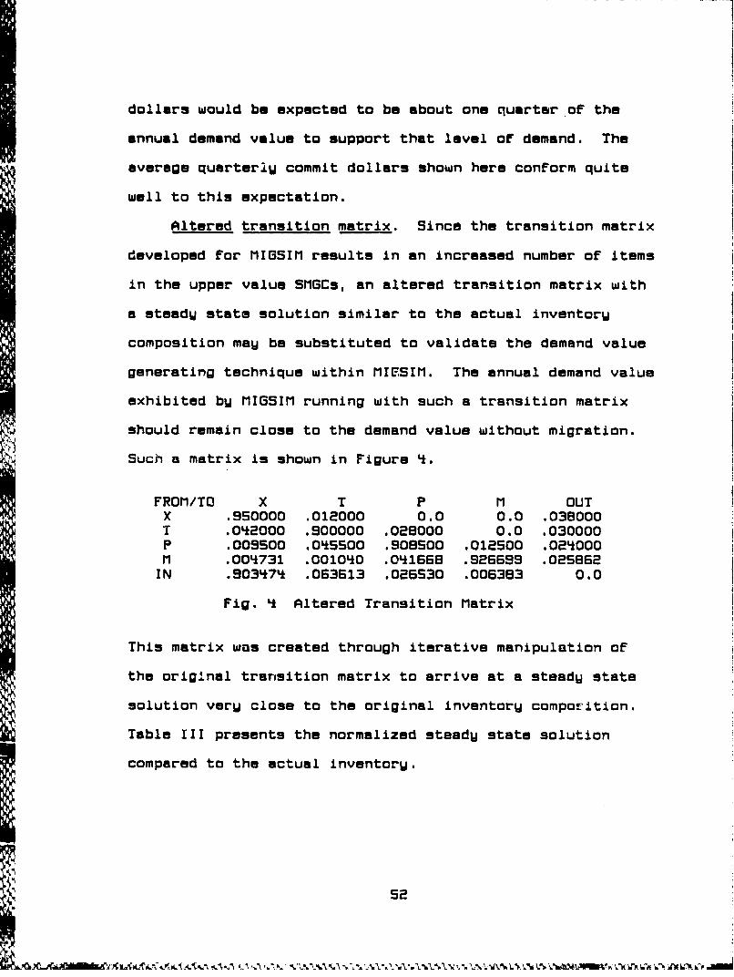
dollars would be expected to be about one quarter of the
annual demand value to support that level of demand. The
average quarter.W commit dollars shown here conform quite
well to this expectation.
Altered transition matrix. Since the transition matrix
developed for MIGSIM results in an increased number of items
in the upper value SMGCs, an altered transition matrix with
a steadW state solution similar to the actual inventory
composition may be substituted to validate the demand value
generating technique within MIESIM. The annual demand value
exhibited by MIGSIM running with such a transition matrix
should remain close to the demand value without migration.
Such a matrix is shown in Figure 4.
FROM/TO X T P M OUTX .950000 .012000 0.0 0.0 .038000T .042000 .900000 .028000 0.0 .030000P .009500 .05SO0 .908S00 .012500 .02000M .004731 .001040 .041668 .8266SS .02S862
IN .903474 .063613 .025S30 .006383 0.0
Fig. 4 Altered Transition Matrix
This matrix was created through iterative manipulation of
the original transition matrix to arrive at a steady state
solution verW close to the original inventory comporition.
Table III presents the normalized steadW state solution
compared to the actual inventory.
52
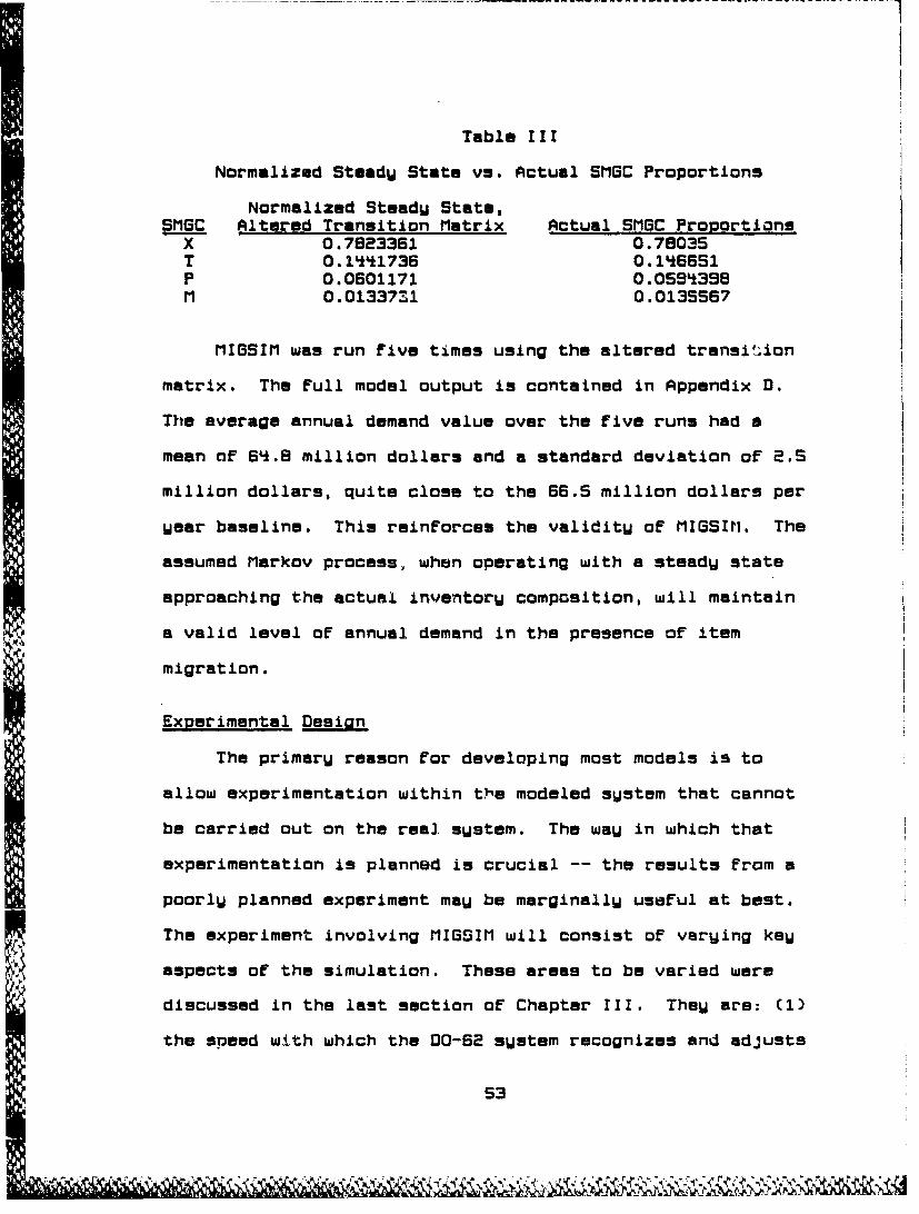
Table III
Normalized SteadW State vs. Actual SMOC Proportions
Normalized SteadW State,SMGC Altered Transition Matrix Actual SMOC Proportions
X 0.7823361 0.78035T 0.1441736 0.146551P 0.0501171 0.05943SBM 0.01337S1 0.0135567
MIGSIM was run five times using the altered transil.ion
matrix. The full model output is contained in Appendix D.
The average annual demand value over the five runs had a
mean of 64.8 million dollars and a standard deviation of 2.S
million dollars, quite close to the 56.5 million dollars per
Wear baseline. This reinforces the validity of MIGSIM. The
assumed Markov process, when operating with a steady state
approaching the actual inventory composition, will maintain
a valid level of annual demand in the presence of item
migration.
Experimental Design
The primary reason for developing most models is to
allow experimentation within the modeled system that cannot
be carried out on the real system. The wau in which that
experimentation is planned is crucial -- the results from a
poorly planned experiment maw be marginally useful at best.
The experiment involving MIGSIM will consist of varying key
aspects of the simulation. These areas to be varied were
discussed in the last section of Chapter III. They are: (1)
the speed with which the DO-B2 system recognizes and adjusts
53
ass- .- O -

to item migration and changing demand, (2) fixed lead time
or different lead time for each SSiiC, and (3) different
values for the implied shortage factor. These are the
factors in the experiment.
Factors. The first factor, the recognition time for
item migration, ham two levels. One is instant recognition
of item migration. All inventory levels are recomputed as
soon as demand changis, and the item is managed according to
its new category. The second level involves a one quarter
lag before DO-S2 recognizes that the item has migrated. For
that quarter, the item is managed according to its old
demand rate, while stock is removed at the new demand rate.
The second factor, lead time variation, also has two
levels. The first employs fixed lead time, assigned
according to SMSC when the item enters the simulation and
never changing throughout the simulation. The second level
allows lead time to change when the item migrates. In this
case, migrating items will receide a lead time equal to the
average lead time of the SMSC they are entering.
The third factor is the i~mplied shortage factor. The
implied shortage factor determines the amount of safety
level present in the inventory. Safety level is an
important method for reducing backorders, and could be of
use in limiting the backorders resulting from item
migration. BW using the implied shortage factor as an
experimental factor, this analysis investigates the ability
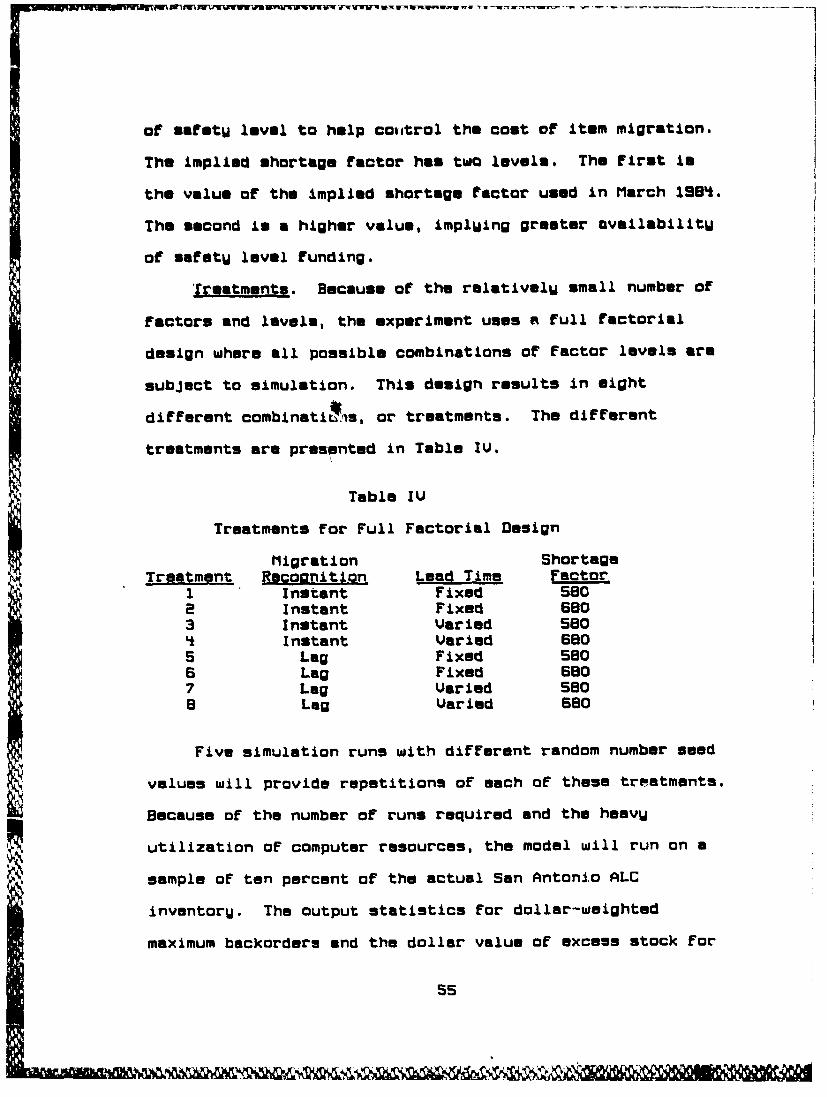
of safety level to help couitrol the cost of item migration.
The implied shortage factor has two levels. The first is
the value of the implied shortage factor used in March 1984.
The second is a higher value, implying greater availability
of safsty level funding.
Treatments. Because of the relativelw small number of
factors and levels, the experiment uses a full factorial
design where all possible combinations of factor levels are
subject to simulation. This design results in eight
different combinatiLls, or treatments. The different
treatments are presented in Table IV.
Table IV
Treatments for Full Factorial Design
Migration ShortageTreatment Recoanition Lead Time Factor
1 Instant Fixed SoInstant Fixed 580
3 Instant Varied 580SInstant Varied 5805 Lag Fixed 5806 Lag Fixed 6607 Lag Varied So8 Lag Varied 680
Five simulation runs with different random number seed
values will provide repetitions of each of these treatments.
Because of the number of runs required and the heavy
utilization of computer resources, the model will run on a
sample of ten percent of the actual San Antonio ALC
inventory. The output statistics for dollar-weighted
maximum backorders and the dollar value of excess stock for
55

items in long supply will be the subject of an analyais of
variance CANOVA) to determine the effect of each of the
factors on the coat of item migration.
i
55
pmam

V. Snhia 2E oaulrs
The MIGSIM computer model was run according to the
mxperimental design discussed in Chapter IV. The output for
all runs is contained in Appendix B. Migration tables from
the five runs are identical under each treatment, and so arm
included for onlU the first treatment. The General Linear
Modal procedure of the Statistical AnalUsis SUstmi (SAS)
provides an analUsis of variance CANOVA) for the output
statistics for dollar-weighted maximum backorders par
quarter and the dollar value of long supplU (15:43S). Thu
results for backorders and long supplU are presented
separatelU, and provide thu foundation for a discussion of
the cost of item migration.
Dollar-Weiohted Maximum nrpra
Table U prnsents the average dollar-weighted backorders
for the first simulation run under each treatment. Refer to
Appendix B for values for runs two through five.
Table V
First Run Dollar-Weighted Maximum Backorders
Migration Shortage Dollar-Weightedftco• i'••L• Lead Time Factor Maximum Backorders
Instant Fixed 580 4,004,050Instant Fixed 580 3,9SS,780Instant Varied 580 4,593,480Instant Varied 680 4,585,730
Lag Fixed 580 10,S63,200Lag Fixed 680 10,94tS.00Lag Varied So 10,753,100Lag Uaried 58O 10,70,800
57
9

Analusis of jariance (ANOVA). The initial ANOUA is of
the Full Factorial design with all possible Factor
interactions. The design is blocked by run number to
compensate For variation caused by the common random number
streams. The Full model ANOVA table with partial sums of
squares, Table VI (page S), shows that interaction effects
are negligible. Of the main effects only the demand
information lag and run number account For signiFicant
variation in the model.
The significance of the information lag and run number
is explored bu reducing the model to onlW the main effects
o? the information lag and run number. Table VII (page 60)
presents the ANOUA table For the reduced model. From Table
UII it is clear that the information lag and variation
between runs account For all significant variaoiiity within
the modpl. The P-values For the partial F tests show that
both Factors are very important. The R-squared value of
0.97 Further shows the modil to be very effective in
explaining variation of responses. Appendix E contains a
plot of predicted values versus Lesiduals which gives no
indication of changing variance, so model aptness is
confirmed. A plot of ranked residuals, also in Appendix E,
supports the underlying assumption of normality. The
strength and validity of this model allow meaningful
analysis of mean responses For Factor levels.
5e
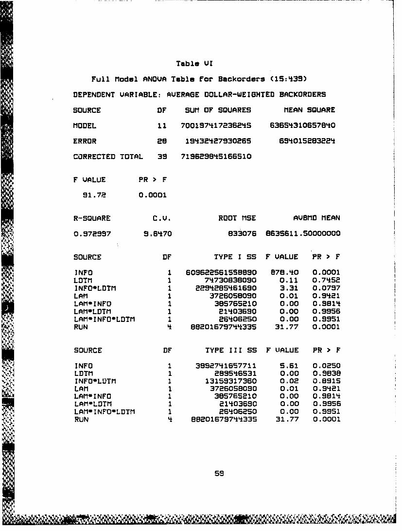
Table VI
Full Model ANOVA Tmble for Backorders (15:439)
DEPENDENT UARIABLE: AVERAGE DOLLAR-WEIGHTED BACKORDERS
SOURCE OF SUM OF SQUARES MEAN SQUARE
MODEL 11 700197417236245 63654310657840
ERROR 28 19432427930265 694015283224
CORRECTED TOTAL 39 7196298*5166510
F UALUE PR > F
91.72 0.0001
R-SQUARE C.U. ROOT MSE AUBMO MEAN0.972997 9.6470 833076 8635611.50000000
SOURCE DF TYPE I SS F VALUE PR > F
INFO 1 609622561558690 878.40 0.0001LDTM 1 74730838090 0.11 0.7452INFODLDTM 1 2294285L61690 3.31 0.0797LAM 1 3726058090 0.01 0.9421LAMOINFO 1 385765210 0.00 0.981'tLAMOLDTM 1 21403690 0.00 0.59556LAMOINFOOLDTM 1 26406250 0.00 0.5951RUN 4 88201679744335 31.77 0.0001
SOURCE DF TYPE III 55 F UALUE PR > F
INFO 1 3852741657711 S.61 0.0250LDTM 1 289546531 0.00 0.9838INFOOLUTM 1 13159317360 0.02 0.8915LAM 1 37260S8050 0.01 0.9S21LAMOINFO 1 385765210 0.00 0.9814LAMOLDTM 1 21403650 0.00 0.9956LAMOINFOOLDTM 1 26406250 0.00 0.9951RUN 4 88201679744335 31.77 0.0001
59
I' KAI

Table UII
Reduced Model ANOUA Tabla for Backarders Cl5:439)
DEPENDENT VARIABLE: AVERAGE DOLLAR-WEIGHTED BACKORDERS
SOURCE DF SUM OF SQUARES MEAN SQUARE
MODEL 5 697824241303225 139564848260645
ERROR 34 21805603B63265 651341290097
CORRECTED TOTAL 39 719629855166510
F UALUE PR > F
217.61 0.0001
R-SQUARE C.V. ROOT MSE AVEMD MEAN
0.969699 9.2737 800838 8638611.SO00000
SOURCE 1F TYPE I SS F VALUE PR > F
INFO 1 609622561586890 950.54 0.0001RUN ' 8820167974433S 34.38 0.0001
SOURCE DF TYPE III SS F VALUE PR > F
INFO 1 609622561556690 950.54 0.0001RUN k 88201679744335 34.3B 0.0001
Comparison of Mean Responses. The MEANS statement
within the SAS General Linear Model procedure provides the
TukeW test for mean response differences and Tukey
confidence intervals for the difference between mean
responses for the two levels of information lag: no lag and
one quarter of lag C15:439). The results appear in
Table VIII (page 61).
60

Table VIII
Mean Responses for Backurders (15:439)
TUKEY'S STUDENTIZED RANGE (HSD) TEST FOR VARIABLE: AVERAGEDOLLAR-WZIGHTED BACKORDERS
ALPHA-.OS DF-34 MSE-6.4E+11CRITICAL VALUE OF STUDENTIZED RANGE-2.874MINIMUM SIGNIFICANT DIFFERENCE-S14669
MEANS WITH THE SAME LETTER ARE NOT SIGNIFICANTLY DIFFERENT.
TUKEY GROUPING MEAN N INFC
A 12539528 20 lag
B 473169S 20 nolag
COMPARISONS SIGNIFICANT AT THE .05 LEVELARE INDICATED BY 'Q'
SIMULTANEOUS SIMULTANEOUSLOWER DIFFERENCE UPPER
INFO CONFIDENCE BETWEEN CONFIDENCECOMPARISON LIMIT MEANS LIMIT
lag - nolag 7293164 7807833 8322502
There is clearly a very large difference in the dollar-
weighted backorders generated when item migration is
instantly recognized compared to a one quarter lag in
migration information. A one quarter lag would seem to at
least double the amount of backorders. A difference of this
magnitude may suggest that P one quarter information lag is
not a very realistic factor level. For instance, iF the
change in demand came from known quantitative requirements,
the projected demand rate would be updated before the demand
actually occurred. Although the item would not migrate for
one quarter. the system would use the updated demand rate to
61

immediatslW compute the correct order size and reorder
level. For the many high demand items falling under the six
month minimum buW policy there is a fifty percent chance of
placing an order in anu quarter, so with a one quarter lag
there is a fiftW percent ch'ance of placing an incorrect
order when migration occurs. Also, a one quarter delay in
recognizing a much higher demand level for such an item will
in itself cause manu backorders, regardless of whether an
incorrect order is placed. But although a one quarter
information lag maW not be entirely realistic, it does
illustrate the importance of accurate, timely demand
information to inventory support.
The importance of the information lag to dollar-weighted
backorders to the exclusion of other factors may be
explained by considering size of the demand change
associated with migration. Safety level, determined bW the
implied shortage factor, provides only a margin of extra
stock to cover demand v&riations about a mean level of
demand during lead time. Item migration to even the next
higher SMGC, creating backorders, often involves at least a
ten-fold increase in demand. A change of this magnitude
overwhelms any reasonable safety level immediatelW,
rendering safety level an ineffective method for
counteracting migration-induced backorders.
The affect of lead time variation is also negliQible,
and for much the same rsason. MIGSIM provides for an
62
ý i~
incrasse in lead time of from 50 to 80 daws when an item
migrates to the next higher SMGC. This adjacent migration
is the most common. A change of that size, when compared to
the length of lead time itself, is not overlW large.
Although it will create some shortfall in stock on hand,
this shortfall, like safety level, will be dwarfed by the
stock shortage resulting from the large demand increase.
Additionally, only orders placed after the item migrates
will be affected by the change in lead time. Orders already
in the pipeline have their own previously scheduled arrival
times which will not change.
The lack of effect of varying lead time runs contrarW
to findings at the Defense Electronic Supply Center.
Research there indicated a significant contribution of
increasing lead time to the backorders caused by upward
migration (1B:9-10). Although the evidence presented here
does not support the same conclusion at AFLC, the reasoning
presented by Smith and Gumbert for the lead time effect is
nonetheless compelling (18:9). The reason for the
inconsistancy between the two studies may be because of the
overpowering effect of the information lag discussed above.
Dollar Value o Lon Supplu
Tab' . IX (page 54) presents the average dollar value of
long supply for the first simulation run under each
treatment. Refer to Appendix B for values for runs two
through five.
63
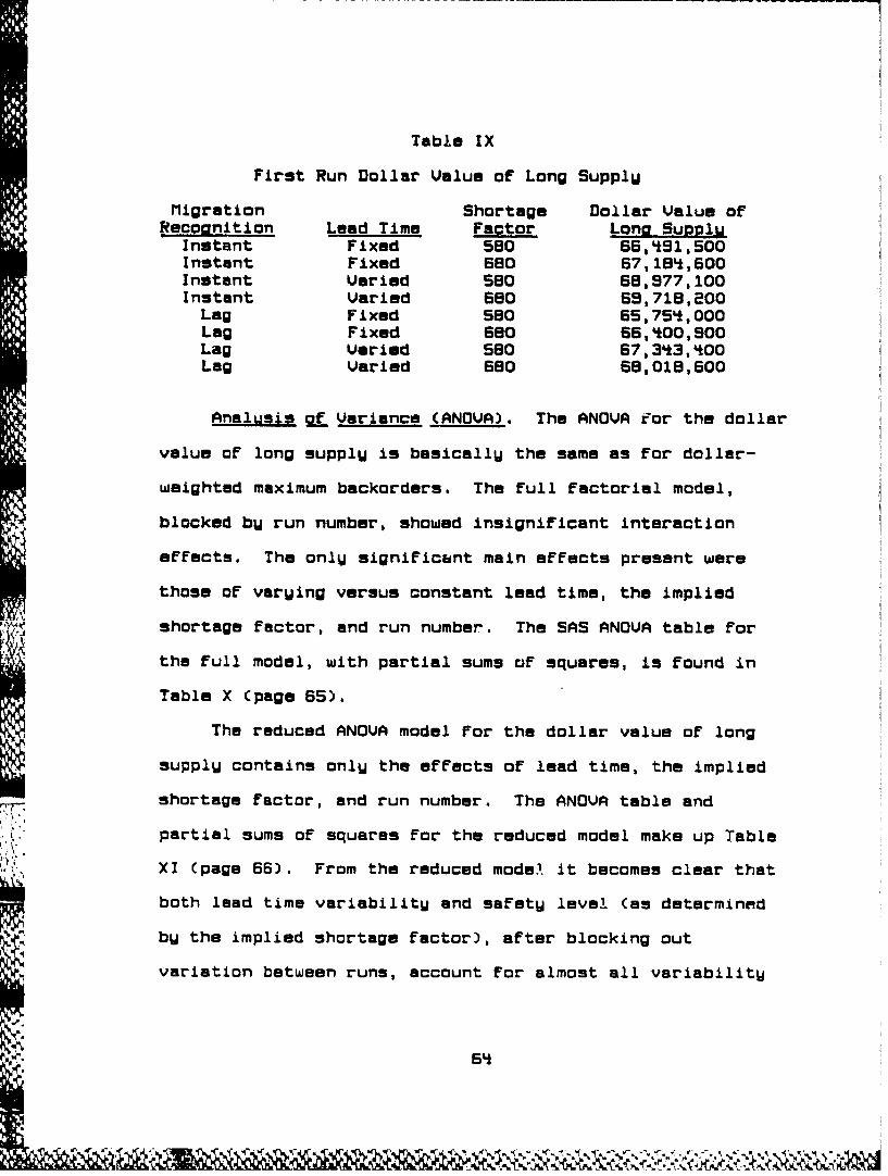
Table IX
First Run Dollar Value of Long Supply
Migration Shortage Dollar Value ofRecounition Lead Time Factor Lono Suoolu
Instant Fixed 580 65,'91,500Instant Fixed 680 67, 18,600Instant Varied 580 68,977,100Instant Varied 680 69,718,200
Lag Fixed 580 5S,754,000Lag Fixed 680 6 5,00,900Lag Varied 580 67,343,400Lag Varied 680 68,018,600
Analusis of Variance (ANOUA). The ANOVUA or the dollar
value of long supply is basically the same as for dollar-
weighted maximum backorders. The full factorial model,
blocked bU run number, showed insignificant interaction
effects. The onlU significbnt main effects present were
those of varying versus constant lead time, the implied
shortage factor, and run number. The SAS ANOUA table for
the full model, with partial sums of squares, is found in
Table X (page 65).
The reduced ANOUA model For the dollar value of long
supply contains only the effects of lead time, the implied
shortage factor, and run number. The ANOUA table and
partial sums of squares For the reduced model make up Table
XI (page 66). From the reduced mode' it becomes clear that
both lead time variability and safety level (as determined
by the implied shortage factor), after blocking out
variation between runs, account for almost all variability
kkil
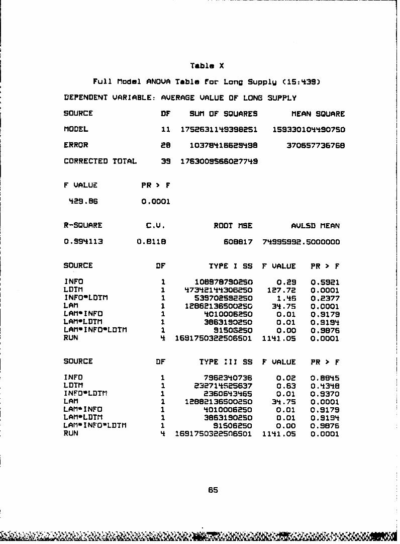
Table X
Full Model ANOUA Table for Long SupplU (15:439)
DEPENDENT VARIABLE: AVERAGE VALUE OF LONG SUPPLY
SOURCE OF SUM OF SQUARES MEAN SQUARE
MODEL 11 1752631149396251 159330104490750
ERROR 2B 10378416629S98 370657736768
CORRECTED TOTAL 39 1763009566027749
F VALUE PR > F
429.86 0.0001
R-SQUARE C.V. ROOT MSE AVLSD MEAN
0.99*113 0.8118 608817 74995992.5000000
SOURCE OF TYPE I SS F VALUE PR > F
INFO 1 106878790250 0.29 0.5921LDTM 1 47342144306250 127.72 0.0001INFOOLDTM 1 539702592250 1.46 0.2377LAM 1 12862136500250 34.75 0.0001LAMOINFO 1 4010006250 0.01 0.9179LAMOLDTM 1 3863190250 0.01 0.9194LAMOINFOLDTM 1 91508250 0.00 0.9876RUN 4 1691750322506501 1141.05 0.0001
SOURCE DF TYPE III SS F VALUE PR > F
INFO 1 7962340736 0.02 0.8845LDTM 1 232714525637 0.63 0.434BINFODLDTM 1 2360643465 0.01 0.9370LAM 1 12882136500250 34.75 0.0001LAM*INFO 1 4010006250 0.01 0.9179LAMOLDTM 1 3863190250 0.01 0.919StLAM*INFOLDTM 1 91506250 0.00 0.9876RUN 4 16917503225O6501 1141.05 0.0001
65

Table XI
Reduced Model ANOUA Table for Long Supply (15:439)
DEPENDENT UARIABLE: AVERAGE VALUE OF LONG SUPPLY
SOURCE DF SUM OF SQUARES MEAN SQUARE
MODEL 6 1751974603313001 291995767218833
ERROR 33 110349627147413 33439280953B
CORRECTED TOTAL 35 1763009566027749
F UALUE PR > F
873.21 0.0001
R-SQUARE C.U. ROOT MSE AULSD MEAN
0.993741 0.7711 578267 74995992.5000000
SOURCE DF TYPE I SS F VALUE PR > F
LDTM 1 47342144306250 141.58 0.0001LAM 1 12882136500250 38.$2 0.0001RUN 4 1691750322506501 1264.79 0.0001
SOURCE OF TYPE III SS F VALUE PR > F
LDTM 1 47342144306250 I41.58 0.0001LAM 1 12882136500250 38.52 0.0001RUN 4 1691750322506501 1264.79 0.0001
in the dollar value of long supplU. The partial F tests
show each to be a strong model component, and the R-square
value of 0.99 attests to the effectiveness of the reduced
model. A plot of predicted versus residual values supports
unchanging variance for model aptness, and a plot of ranked
66
residuals confirms that the assumption of normality is
valid. Further analysis of mean responses is warranted.
Comparisonof Moan Responses. Again, SAS provides the
Tukey test for significant differences between mean
responses for each level of a given factor. The TukeW
confidence interval for the diffnrence between mean
rosponses is also included.
The difference in the dollar value of long supply for
constant and varying lead time is shown in Table XII. Both
the mean difference and the 95 percent confidence interval
show a considerable increasra in long supply when lead time
varies. The higher safety level associated with a higher
implied shortage factor also brings about a higher mean
response in the dollar value of long supply, as shown in
Table XII (page 66). While the effect of safety level is
roughly half that of varying lead time, it is nevertheless
significant.
The reason for the considerable effect of lead time
changes on long supply involves the direct relationship
between lead time and the Approved Force Acquisition
Objective (AFAO). A major portion of the AFAD is the
reorder level, which in turn is primarily a function of lead
time. It is reasonable to expect lead time to fall when
demand falls. Less demand means smaller orders, and smaller
orders take less processing time and are not subject to as
many restrictions to assure competitive purchases.
67

Table XII
Mean Responses for Long Supply (15:43S)
TUKEY'S STUDENTIZED RANGE (HSD) TEST FOR VARIABLE: AVERAGEUALUE OF LONG SUPPLY
ALPHA-.O5 DF-33 MSE-3.3E÷1CRITICAL VALUE OF STUDENTIZED RANGE-2.877MINIMUM SIGNIFICANT DIFFERENCE-37204S
MEANS WITH THE SAME LETTER ARE NOT SIGNIFICANTLY DIFFERENT.
TUKEY GROUPING MEAN N LDTM
A 7608390S 20 vary
B 73906080 20 fixed
TUKEY GROUPING MEAN N LAM
A 75563490 20 Goo
B 74428435 20 So
COMPARISONS SIGNIFICANT AT THE .05 LEVELARE INDICATED BY ,**'
SIMULTANEOUS SIMULTANEOUSLOWER DIFFERENCE UPPER
LDTM CONFIDENCE BETWEEN CONFIDENCECOMPARISON LIMIT MEANS LIMIT
vary - fixed 1803780 2175B25 25*7870
SIMULTANEOUS SIMULTANEOUSLOWER DIFFERENCE UPPER
LAM CONFIDENCE BETWEEN CONFIDENCECOMPARISON LIMIT MEANS LIMIT
680 - S5O 762950 113LkSS 1507040
Production oF smaller orders takes less time as well. If
lead time falls with demand, not only is the AFAO decreased
as a result of declining demand, but it is also decreased by
66

declining reorder level. The lead time "pipeline" becomes
shorter and lessn stock is needed to meet the AFAO. lior.
stock falls above the AFAO and is counted as long supply.
Higher lmv~ls of safety stock contribute to an
increased dollar value of long supply by increasing the
amount of stock on hand when an item mi~rates downward. Low
demand value items are likely to have little or no safety
level for am reasonable implied shortage factor value. An
item migrating downward takes along its safety level to the
lower demand level, where the safety level requirement is
reduced or eliminated. The former safety stock is no longer
part of the reorder level and so is not needed to meet the
AFAG. It only adds to the excess stock over and above the
AFAD.
The lack of~ effect of a demand information lag on the
dollar value of long supply can be explained by the size of
the drop in demand that occurs when an item migrates
Idownward. Item demand drops considerably, and stock on handis reduced at a much smaller daily rate, whether or not theinventory management system recognizes that migration hasII occurred. So in the presence of an information lag, while
then reorder level is set too high For one quarter, it is
unlikely that the new lower demand rate of the downward
migrating item will cause that reorder level to be breached.
Only in those instances where the item is alreadW close to
69

the reorder point when demand drops will an incorrsct order
be generated because of the information leg.
Dollar-WeiAhtmd W5yim §Dackorders. Analusiz of the
results of MIGSIM provides a best and worst case scenario
for the dollar-weighted backorders generated by item
migration. The best case is when the demand change
resulting from item migration is recognized instantly,
allowing an average of about *.7 million dollars worth of
backorders per quarter. This measure of backorders does not
take into consideration the importance of specific
backorders. Certainlu backorders of a high-prioritU part
which mau ground a weapon sustem are much more costlU to the
Air Force than backorders of office supplies. MIGSIM does
not measure the prioritU of a backorder.
The steadu state solution for the MIGSIM transition
matrix may also influence the cost of migration. The
gradual growth in demand value predicted by the steadu state
solution and observed within MIGSIM means more items may be
migrating to higher SMGCs than in the actual inventory
sustem. Increased upward migration would tend to inflate
the value of backorders observed.
The dollar-weighted backorders present under the one
quarter demand information lag, as mentioned earlier, may
not relate to a realistic inventory scenario. Large
increases in demand mau come from quantitative requirements,
70
which would be known in advance by the system and added to
the predicted demand before demand actuallu changes. But
the dramatic increase in backordars resulting from the delaU
does illustrate the crucial role accurate information on
Item demand plaUs in determining the effectiveness of an
inventoru system. The cost of item migration in terms of
dollar-weighted backorders is clearly substantial, even with
the most timmlu information on item demand.
Dollar Ualue of Long SuoPlu. To effectively gauge the
value of long supplu caused by item migration, the excess
stock present during migration must be compared to the
excess stock already in the inventory. The level of
existing long supplU can be observed from the MIGSIM run
with no item migration contained in Appendix C. The average
value of that baseline excess stock is about 29 million
dollars. Item migration creates 74 to 76 million dollars of
long supply depending on the amount of safety level and the
variability of lead time. It appears that item migration
may be responsible for increasing the value of long supply
over 45 million dollars during the twelve quarters of the
simulation. If this number 13 extrapolated from the ten
percent inventory sample to the entire inventory, the figure
could be roughly 450 million dollars. That is a large
amount of munew tied up in unnecessary stock -- money thatcould be used to meet priority requirements elsewhere. The
71
cost of item migration must include this opportunlitu cost of
funds committed to unneeded stock.
-7
VI. Conclusions end Recommendations
Conclusions
Item migration has been shown to exist in inventory
systems within the Department of Defense. But though the
occurrence of item migration was documented, the full
implications of item migration for inventorW managers were
not explored in depth. No cost was assigned to item
migration eit'her in terms of dollars or a decreased ability
of the inventory to meet the needs of customers.
This research effort begins to quantiFy the effects of
item migration on the AFLC consumable item inventory. A
simplified model of the inventory management system provides
a vehicle to measure both the value of backorders generated
by items migrating upward and the value of stock in long
supply created by items migrating downward. The influence
of certain key factors within the inventory management
system are analyzed. These factors are the speed with which
the system recognizes and reacts to the demand change
resulting From item migration, the variability of lead time,
and the amount of safety level in the inventory.
It appears that the ability of the inventory system to
react quickly to large demand changes is very important in
limiting the number of backorders from upward migration.
The chance of failing to place a necessary order of
replenishment stock or placing too small an order before the
system adjusts to the now demand rate greatly exacerbates
73

the problem oF backorders. The research investigated only
the ability to react once migration occurred, however, not
the effect of correctly anticipating item migration before
it occurs. On the other hand, reaction time during item
migration is not important for downward-migrating items.
The sudden drop in demand occuring when an item moves to a
lower SMGC makes the breach of the reorder level unlikely,
even if the reorder level is calculated from a higher,
incorrect demand rate. So incorrect orders of stock seldom
result,
Lead time variability seems to have little effect on
migration-induced backorders. The large demand change
associated with migrating to a higher SMGC may overshadow
the extra stock required in the "pipeline" for increased
lead time, at least when lead time increases only
incrementally as within this model. As mentioned in Chapter
IU, this lack of effect runs counter to the findings of
Smith and Gumbert at DESC (18:9). The disagreement may be
reconciled by realizing that the large information lag
effect may render an otherwise valid lead time effect
invisible. However, lead time changes have a definite
effect on the amount of long supply resulting From downward
migration. As lead time decreases, so does the Approved
Force Acquisition Objective. Stock that before was Filling
.'the lead time "pipeline" is no longer required for that
purpose, and adds to the amount of long supply.
74
The last factor, the implied shortage factor,
determines how much safety level is present. SafetW level
is shown to be ineFFective in limiting backorders From item
migration. The large demand change associated with upward
migration overwhelms the relatively small margin of safety
stock. Safety level does influence the value of long
supply, for much the same reason as varying lead time.
SaFety level counts toward the Approved Force Acquisition
Objective. At lower demand levels less safety stock is
required, and the Former safety stock winds up adding to the
amount of long supply. The higher the safety level, the
more the potential for long supply.
This research effort attempts to put a "price tag" on
item migration. The figures arrived at, however, must be
couched with the realization that approximations within the
model may affect the magnitude of the cost. The model shows
a mean dollar value of maximjm backorders of 4.7 million per
quarter under the best conditions, i.e. with instant
Srecognition of item migration. This figure may be inflated
by the general rise in total demand value for the entire
inventory as the model approaches the Markov steady state.
But even in light of that fact, it may be safely said that
item migration causes large amounts oF backorders, and the
failure of inventory management to react quickly to changing
demand will greatly increase the level of backorders. This
is illustrated by the jump to a mean of 12.S million dollars
75

in backorders per quarter when one quarter is allowed to
elapse before the inventory management system recognizes the
now demand level.
The v'alue of long supply is less volatile in responding
to different levels of the factors influencing it. The mean
responses range from about 7'4 to 76 million dollars worth of
stock. While this difference is statistically significant,
when compared to the overall amount of long supply it
carries less weight. Although reducing safety level would
produce a lower value of long supply, the increased
backorders resulting from the routine demand fluctuations
of moe idUp in this level of long supply is lamentable,
but the factors investigated here do not provide a solid
* basis for attacking the problem. While the effects of
varying lead time and safety level pass the significance
test, they do not have the magnitude necessary to spawn new
management policy.
The cost of item migration shown in the model may be
extrapolated to the entire San Antonio ALC inventory. The
model was run on a ten percent sample, so multiplying the
results by ten indicates the effect on the whole consumab'les
inventory. Item migration may account for at least Lj7
million dollars in backorders each quarter in just this one
ALC, and if similar conditions exist in the other- four ALCs,
the backorder cost to AFLC becomes greater still. The
K), 76

calculated value oF migration-induced long supply at San
Antonio ALC is about 4SO million dollars over a three. ear
period. Again, if this is similar to the other ALCs, AFLC
is experiencing great opportunity cost as a result of item
migration. As new weapon systems enter service and the
defense budget becomes tighter, the money tied up in long
supply will be urgently needed to meet priority
requirements. The cost of the long supply shown here maw
become intolerable.
RecommendationsI The research presented here has provided some insight
into the movement of items betueen SMGCs and the impact of
that phenomena on the inventory system. The most
meaningful Finding is that item migration costs money, and
good, responsive inventory management can limit that cost.
AFLC would be well served by investing resources in ways to
quickly recognize the large increases in demand that
indicate item migration. The sooner the item is managed
according to the new demand level, the fewer the resulting
backorders. Accessible, accurate data on projected
requirements will greatly aid in this area, The
Requirements Data Base initiative, now becoming operational
in AFLC, is just the mechanism to provide such data.
The impact of item migration on inventory mansjement
policies must also be considered. This research shows that
much oF the long supply present is the result of downward
77
migration. Any action taken to evaluate or prevent long
supplW must be directed at downward-migrating items.
Minimum buy policies may also be confounded by item
migration. AnW increase in the minimum buy will increase
the average size of the inventoy7, and the resulting extra
stock will further increase the amount of long supply from
downward migration.
While answering some questions, this research has also
uncovered new questions. AnalWsis of the characteristics of
items in each SMGC shows great disparity within SMGC X. The
overwhelming majority of X items have no demand. The
parameters of the zero demand items are far different from
their positive demand counterparts in SMGC X, yet all are
managed as low value items. For instance, the prices for
zero demand items in general are much higher than for other
X items. Since zero demand items make up such a large part
of the inventorW, the nature of these items should be more
thoroughlW explored. It maW be interesting to know where
these items originated, how long theW have had no demand,
and the probability of experiencing demand in the future.
Finally, the manner in which items migrate should be
investigated Further. The model used for this research gave
all items in an SMGC an equal chance of migrating. This was
necessarW since the onlW data available provided onlW a
count of items moving between SMGCs. It maW well be that
items tend more to migrate between the upper range of one
78
J 4A .A

SMGC and the lower range of the next highest VIGC. Given
the breadth of the uppeo SMGCs such a Jump could still
involve a large demand change, but not the average ten-Fold
increase For upward migration currentiW experienced in the
simulation. Better understanding of the specific origins
and destinations of migrating items will allow more accurate
modeling of migration in the future.
I
79
w N

Appendix A: tIIGSIM FORTRAN Source Code
60

C Program MISSIMC Variables:c cat - SMSC CX-l,T-2,P-3,rl-',OUT-S)c q -economic order quantityc al - safmtu levelc rol -reorder levelC leadti - lead time (dayus)C ip -invantoru position Con hand plus due in)C pmdr - program monthlW demand ratec demand - dollar value of~ annual demandc lam - implied shortage factorC astot -total on hand ass3etsc price - actual unit pricea mad - mean absolute deviation of~ demandC ers - average requisition sizec ppr - peacetime program ratioc lag -is there a one quarter information lag? CT/F)c varldt -doss lead time varw bW SMGC? CT/F)c migad - seed value for migration generatorc demsd - seed value For demand generatorc av** - average of quarterly values fora output statisticcU mgcnt migration tables
c bkrd -backorder daysC bkmax - maximum backordersc bkdol, dollar-weighted bacnkorder daus
c bkmxdl - dollar-weighted maximum backorder da~sc longsp - number of' items in long supplua longdl -dollar value of' long supplUC demval -toital annual demand valuec comdol - quarterlU commit dollarsC qtrdue - quarter dk.9 of' inbound orderC daUdue - daW due of' inbound ordera order - size of' inbound ordera mprob - cumulative transition matrixa madval - average mad value f'or each SMGCc arsval -average ars value f'or each SMGCc prval -empirical price distribution f'or each SMGCc
program migsim
&bkord(12),bkmax(12),ldtvalC'*),qtrdue(6),&daudue(6),order(S),q,rol~leadti,run,ip,&longspC l2)integer migsd, dmsd
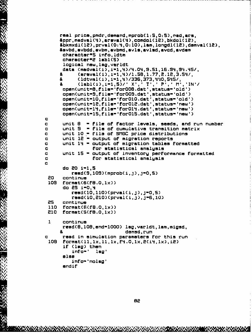
* ~real pricm,pmdr,dumand,mprobC1:5,0:5),rmad,ars,&ppr,madvalC'k),arsvalC't),comdol(12),bkdol(12),&bkmxdl(12),prvalC0:'t,O:10),Iam,longdll(l2),clemval(12),&avbd, avbdd,avbm, avbmd, avis,aviud, avcd,avdmmcharacter*S info, ldtmcharmctur*2 lablC5)logical e, lag, varldt.dataCmvai),i1)/.Ok.5,69.i5/
a Ceraval~i), 1-1, 4)/3365,1373, 442,3.5*/,& (labl~i),i-1,5)/' X), ,TO,$ ?PI,$ MP'W(dvl/,-,*/3633''05k/open(unit-B,rile-'ForOOB.dat' ,status-'old')open~unit-S,File-'forOOS.dat' ,status-'old')open~unitl10,file'lforOlO.dat' ,status-'old')open~unit-12,rile-'EorOl2.clat' ,status-'new')open~unit-1'i,fil.-'For~l'*.dat' ,status-'new')open~unit-15,Filein'Eor015.dat',status-mnew')
c unit 8 - file or rector levels, seeds, and run numberC unit 5 - rile of cumulative transition matrixc unit 10 -fila or SMSC price distributionsc unit 12 - output of migration reportsC unit 14* - output of migration tables formattedc for statistical analysisc unit 15 - output of inventory performance formattedc ror statistical analysis
do 20 1i1,5readC5,10S)Cmprob~i,j) ,J0O,S)
20 continue109 formatCBSfB.O,1x))
do 25 1-0,4*read(10,110)CprvalCi,j),J-0,5)read(10,210)Cprval~i,j) ,J-6, 10)
25 corntinue110 formatC6CFB.0,lx))
210 formatC3CFB.O,lx))II1 continuereedCB,1O8,end-1000) lag,varldt,lam,migsd,
& demsd,runc read in simulation parameters for this run10B format~ll,lx,11, lx,f'*.O,lx,2Ci*, lx),i2)Iv: if C(lag) then
into-' lag'else
info-' nolag'endif
82

~~~~~~~1~~~~~~ ----------------------- --------- 1
If Cvarldt) thenldtm-' varu'
alga
1dtm-'Fixed'endif
do 5 1-1,12bkord(i)-Obkdol(i)-Obkmax(i)-Obkmxdl(1)-Olongsp(±)-Olongdl(i)-OdemvalCi)-Ocomdol(i)-Odo 10 J'1,5
do 15 k-1,5mgcnt~i,Jk)-O
15 continue10 continue5 continue
new-.False.
write(12,113)if (lag) then
write(12,114)also
write(12,115)endifif (varldt) than
write(12,116)else
write(12,117)endifwrite(12,120) lamwrite(12,118) runwrite(12,119) migsd,demsd
c write header for run output113 format(C '/' sI' / ','Model output'/)114 format(' ','One quarter information lag')115 format(' ','No information lag')116 format(' ','Uariable lead time')117 format( ','Constant lead time')118 format ','Run number ',12)119 formatC ','migsd- ',14/' ','demsd- ',i4/)120 format(' ','Implied shortage factor- ',f4.0)
open(unit-1l,file-'fcrOll.dat',status-'old')c unit 11 - file of inventorU items
2 continuereadC11,111,end-900) price,astot,ppr,pmdr,l d':i,
a mad,arm
63
4.... ......

if (price.eq.O.0) goto 2dommnd-prica*pmdr*12. 0
C categorize into SMGC9if (domand .gm.O.and .demand. lu.S00.O) than
cat-11endifif (dmmancl.gt.500.0.ancdadmand.la.5000.0) then
cat-2endifif (clamand.gt.S000.0.and.demartd.le.50000.0) then
cat-3endifif Cdemand.gt.S0000.0) than
cat-,*endifif' (ppr.eq.0) ppr-l.0leadti-ldtval~cat)1.adti-nintCCleaacti/355.O)036'*.0)if Cmad.eq.0) mad-madvai~cat)if Care.eq.0) ars-arsval~cat)qtrl1if (demand.ne.0) then
call buUdum~pricm,astot~ppr,pmdr,leedti,mad,ars,& qtrdum~daUdue,ordur,q,rol~lsm,new,& comdol.ip~qtr,cat)
elseip-matot
rolO0do 35 i-1,6
or-dmr( i)-0qtrdu. i )-0daudue~i )0
3S continueendifcall cUclm~qtr,cat,mgcnt~mprob,price,astot,ppr,a pmdr,leadti,mad,ars,demand,migsd,demsd,a madval ,arsval,bkord, bkdol, bkmax, bkmxdl,a comdol, qtrdue, daydue, order, q,rol,new, lag,a&ot varldt,lam, longsp,longdl,damval,ip,ldtval)
900 continue
a migsd,dumsd,bkord,bkclol ,bkmax,bkmxdl,
writs(l2,121) ido S10 J-1,5
writ.C12,112) lsblCj),Cmgcntci,j,k),k-1,S)
writae'*14,11) info,ldtm,1.rn,run,i,j,I & (mgcnt(i,j,k),k-1,5)

910 continuewritec 12,500)
920 continuec compute average of quarterly stats
avbdd-0avbmdinOavbm-0avismdOavladin
avcd-0mvdam-0do 930 i-1,12
avbd-avbd~bkord Ci ) /12.avbdd-avbdd+bkdol Ci) /12.avbm-avbm~bkmax i )/12.avbmdinavbmd+bkrnxdlCi )/12.mvls-avlu+longup( i )/12.avlsdinevlsd+IongdI~i )/12.avcd-avcd+comdol Ci) /12.avdam-avdemedemvel Ci) /12.
930 continuewrita(l2, 212)do960 1-1,12
write(12,312) i,bkcrd~i),bkdol~i),a bkmax~i),bkmxdl~i)
960 continuewrl~teC12,313)writeC 12, 31') evbd,avbdd,svbm,avbmdwriteC 12,500)writeC 12,4'12)do 970 1-1,12
write(12,'*13) i~longsp~i),longdl~i),comdol(i),* uiemval(i)
970 continuewrite C12,313)writeCl2,'*1') avlsaevlsd,evcd,avdamwriteCl5,151) info,ldtm,lam,run,avbd,avbdd,avbm,avbmd,a avls,avlsd~evcd,avdemcloseC 11)goto 1
C get next item111 rormattrll.0,lx,iS~lx,rS.O,lx,rlo.0,lx,
a i5,1x,f11.O,1x,F7.0)112 formatC' ',aE,3x,5CiB,2x))121 formatC' ','Quarter ',12/
I 9,'FROM/TO X',Sx,'T',Sx,'P',Hx,& M',Bx:,'DUT')
14*1 Eormet(' ',2Cm5,lx),r'*.0,lx,3Ci2,lx),S~i6,lx))151 formatC' a,2CmS,1x),f'*.0,1x,i2,lx,*Ce12.6,lx)/
& ' ',*Cel26,lx)
ININ -I IW. 100185l
Khan I -I-
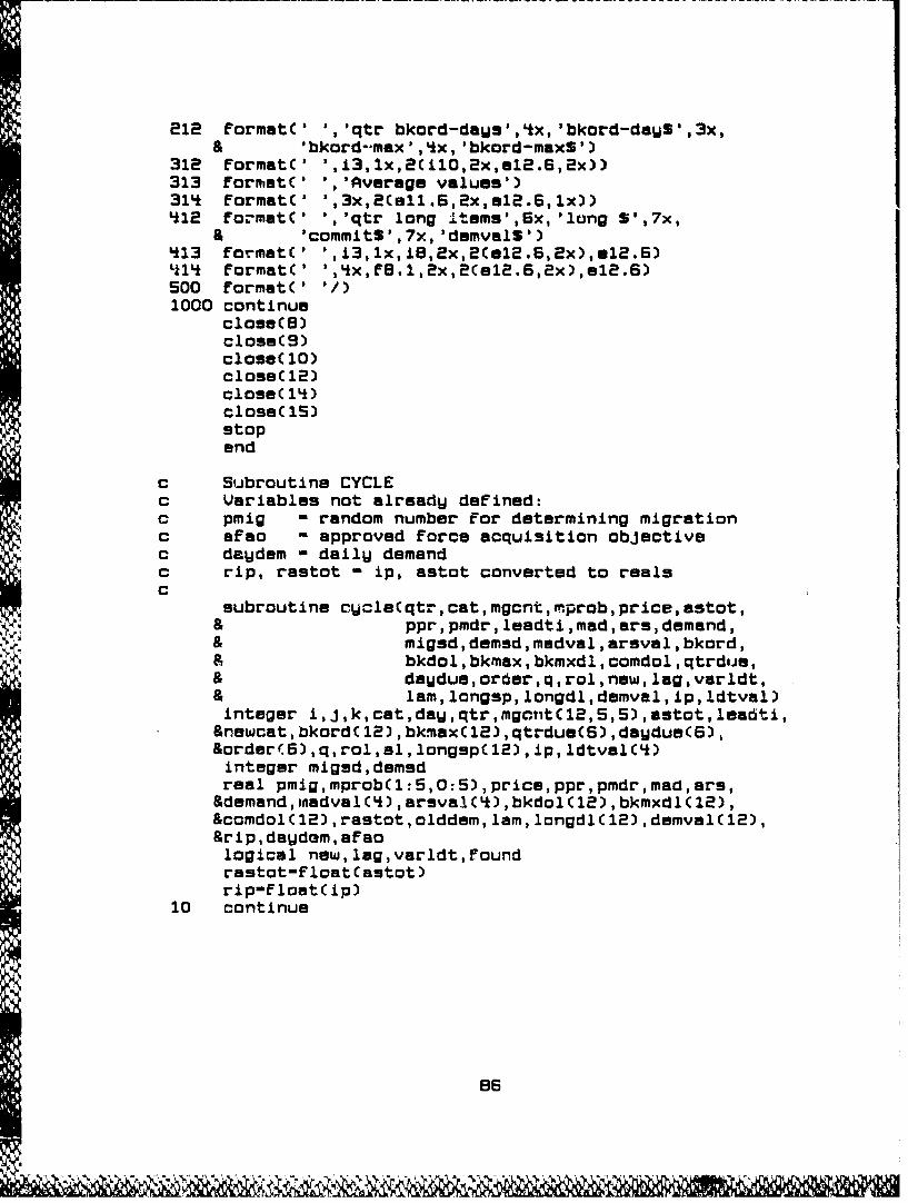
212 format(' ','qtr bkord-da~s' ,4~x, 'bkord-daUS' ,3x,a *bkord--maxI ,4'x, 'bkord-maxS')
312 format(' ',i3,1x,2(i10,2xm1l2.6,2x))313 format(' ','Average values')314* format(' ',3x,2Ce11.6,2x,e12.6,1x))41l2 for~mat(' ','qtr long .1tems',6x,'long S',7x,
a 'commit5',7x, 'dmmvalS')413 fromat(' ',13,lx,iB,2x,2Cel2.S,2x),el2.S)4k14 Format(' ','kx,f8.1,2x,2Cel2.6,2x),e12.6)500 formatC VI)1000 continue
close C8)closeCS)closeC 10)closeC 12)close C1'i)closeC 15)stopend
c Subroutine CYCLEc Variables not already defined:c pmig - random number for determining migrationc afac - approved force acquisition objectiveC daydem - daily demandc rip, rastot - ip, astot converted to realsC
subroutine cycle~qtr,cat,mgcnt,'!~prob,price,astot,& ppr,pmdr,leadti~mad,ars,demand,& migsd,demsd,madval,arsval,bkord,
& ~bkdol,bkmax, bkmxdl,comdol ,qtrdue,& daydue,orcder,q,rol,new,lag,varldt,
& ~lam,longsp, longdl,demval,ip,ldtval)integer i,.j,k,cat,daW,qtr,mgcntitl2,5,5),astot, leadti,&newcat,bkordC 12) ,bkmax(12) ,qtrdue(5) ,daydue(6),&orderC6),q,rol,sl, longsp(l2),ip, ldtvalC(k)integer miged,demsdreel pmig, mprob~l :5,0:5) ,pric., ppr, pmdr, mad, ars,gdemand,madvalcl*),arsvalC(k),bkdol(12),bkmxdl(12),&comdol(C12), rastot, aiddum, lam, longdl(C12) ,dumval(C12),&rip, daydom, afaological new, lag, varldt, Foundrastotinfloat Castot)rip-f lost Cip)
10 continue
86

c generate item migrationif C4tr.le.12.and.cat.ne.S) then
if C.not.new) thenpmig-ran( migad)do 15 k-1,S
if Cprnig.ge.mprob~cat,k-1) .and.pmig.lt.& mprob~cat,k)) then
newcatmkandif
continuemgcnt(qtr,cat, newcat)-mgcnt~qtr, cat, newcat)+1
elsenewcat-catmgcnt Cqtr,5, newcat )imgcntC qtr,5, newcat) +1new-. false.
endifif Cnewcat.ne.5) then
olddemindumandif (cat.ne.newcat) then
if Cvarldt) leadti-& ~nintC(ldtval(newcat)/365. )*35L*.)
c get new demand levelcall getdem~newcat, demsd, demand)pmdr-(demand/prica)/12 .0if Colddem.eq.O.or..not.lag) then
if CBFs.eq.0) ars-arsval(neuwcat)if Cmad.eq.O) mad-madval~newcat)
c compute levels For instant reactionIc to item migration
call levelcnewcat,demand,q,sl,rol,price,
&ni pmdr, ppr, mad, leadti ,ars, lam)endif
da~demin(pmdr*12.0)/3S4*.0do 20 dayl1,S1
do 25 i-1,6if Cqtrdue~i).eq.qtr.and.daydue~i).eq.day)
& thenc when order arrives count max backor-ders
if Crastot.lt.0) thenbkmax~qtr)-
& bkmax~qtr)+nint~abs~rasto.;))bkmxdl Cqtr)-
a bkmxdl Cqtr)+abs(r3stot~price)andi10'rastot-rastot+orderC i)order~i)inOqtrdum~i )iOda~due~i )iO
endif2S continue
87

rastot-raatot-daudumrip-rip-daudum
c count backorder daysif (rastat.lt.0) then
bkord(qtr)-hko-6d(qtr) +- nint(abs~rastat))bkdol~qtr)aubkdo1Cqtr)4+ abs~price*rastot)
endifif Crip.lm.rol) then
c place and 3chedule orderi-1found. False..
3S continueif(i.le.5.and. .not.found) then.
if Corderci).eq.O) thenorder i )-q+(Crol-nint(rip))qtrdua~iýinqtr~int~leadti/91 .)
& ~~int(day/9l .0+-leadti/S1 .0-& int~leadti/Sl.))
daudu9(i)-1+mod('leadti+daw, 91)comdolCqtr)-
& ~comdol Cqtr)+CorderC i)*price)rtp-rip4-orderC i)found-. rue.
endifi-i+e-goto 3S
andifendiF'
20 continue
if' Ccat.ne.newcat.and.lag) thenc compute levels after one quarter lag
call level~newcat,demanii,q,sl,rol,price,& pmdr, ppr, mad, leadti ,ars, lam)
endif'
andif'
cat-newcatdemval&(qtr)-demval~qtr)-edemand
c count items and value of' long supplWif' Ccat.eq.1) then
aF'ao-'rol~q+Cpmdr*1R .0)alse
af'ao-rol~amaxi~f'loat(q), (pmdr*2'.0))endif'if' Crip.gt.af'ao) then
longspC qtr )-lavrtspC qtr )+1longdl~qtz-)-longdl~qtr)+price*(rip-af'ao
endiF'

qtrinqtr+ 1Goto 10
endifastot-nint Crastot)ip-nint~rip)return
c ou - nmbe of tem leai inin a quarter
C frcdn fratio of tem toenter a SMGC that have
a arsval,migsd,demsd,bkord,bkdrnl,& bkmax,bkmxdl,comdol, longup, longdl,& demval, lag, varldt, lam)real mprob(l :5,0:5) ,prvalC0:'*,0: 10) ,madvalC'*),
&arsvalC*) ,bkdol(12) ,bkmxdl(l2) ,comdol(l2) ,longdl(l2),gdemvalC 12) ,laminteger ldtvalC(k),mgcnt(12,5,5),bkord(l2),bkmax(12),
&longspC 12)integer migsd,demsdreal fracdn,price,demand,pmdr,ppr,j,med,arsinteger qtr,cat,i,k,totlin,astot, leadti,sl,rol,q,
&qtrdue(6),da~dueC6),orderC6),qstart,out,ip,ii,&numin, catstlogical found, new, lag, varldtdo 50 qtr-1,12
out-0c count items that left SMGC
do 4*5 k-1,4outinout+mgcnt~qtr, k, 5)
'*5 continuetotl in-outif Ctatlin.gt.0) then
do 4*0 catl1,'c calculate number to enter each SIIGC
& ~numin-nintCfloat~totlin)*CmprobC5, cat)-a mprob(S,cat-i)))
if Cnumin.eq.0) numininldo 30 i'1,numin
c track how manu have entered alreadWfracdn-float i )/Float~numin)J-0o.1found-. False.
20 continue
89
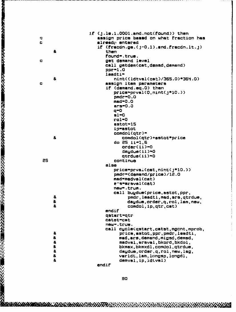
if (J.lm.l.0001.and.not(found)) thenC assign price based on what fraction has
C already' enteredif Cfracdn.ge.(J-O.l) .mnd.fracdn.It.j)
& thenfound- . rue.
C get demand levelcall getdom( cat, demsd, demand)ppr-1 .0laadti-
& nint( Cldtval~cat%-)/365.O)*36Lk.0)c assign item parameters
if Cdomand.sq.0) thenprice-prvalC0,nint(j*l0.))pmdr-0.0madO .0ars-O .0q-0
rolO0astot'15ip-astotcomdal~qtr)-
a comdol (qtr)+astot~pcicedo 2S 11-1,6
order( ii)-0daUdue~ii )-0qtrdue( ii )0
25 continuealso
price-prval~(cat,nintQj010.))pmdr-(domand/price)/12 .0madinmadvsl (cat)-s-arsval (cat)
new. trun.call buUdueC price, astot, ppr,
& ~pmdr, leadti ,m, ars, qtrdue,a da~due,order,q,rol,lam~now,
& ~comdol, ip,qtr,cat)endifqstart-qtrcatst-catnew- . rue.call c~cle~qstart, catat, mgcnt, mprob,
& ~price, astot, ppr, pmdr, leadti,& ~mad, ars, demand, migad, demsd,I & madval ,aruval, bkord, bkdol,a ~bkmsx, bkmxdl, comdol ,qtrdue,
a da~due,order ,q, rol,new, lag,& varldt, lam, longap, longdl,a&ni demval, ip, ldtval)
so

i-i +0.1goto 20
endif30 continue4*0 continue
anclif50 continue
returnand
c Subroutine BUYDUEc Variables not already defined:c dumin - number of days before order is due inc from start of item in simulationc PCP - procurement cycle period0 numord - number or orders to be scheduledc
subroutine buudue~price,astot,ppr, pmdr, lemdti ,mari,ars,a qtrdue,de~due,order,q,r-ol,lam,new,a comdol,ip,qtr,cat)real price,ppr,pmdr,mad,ars,lam,comdol(12),demandinteger astot,leadti,qtrdueC6),da~dueC5),orderC6),
&sl ,q, rol ,dusin(6), ip,qtr,cat, pcp, i, numordlogical newdemand-pritce~pmdr*1B .0call level~cat,demand,q,sl,rol,price,pmdr,ppr,a mad,leadti,ars,lam)pcp-nint(cq/Cpmdr*12 .0/364*.0))if (newu) then
astot-q+s 1comdol Cqtr )-comdol Cqtr ) price~astot
elseir Castot.le.sl) astot-q+sl
endifip-astotdo 10 1i1,6
duein~i)0Oorder~i)inOqtrdue~i )0daUdueC i )0
10 continuec see if an order is needed within lead time
dusinC1)-nintC(astot--sl)/Cpmdr*12.0/36'*.0))if Cduein~l).lt.leadti) then
C see how meny orders needednumord-intC Cleadti-duein 1) )/pcp)I if Cnumord.gt.0) then
1A4 iftnew) comdol~qtr)-comdol~qtr)+numor-d*q*price
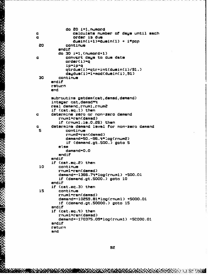
do 20 £-1,numordc calculate number of da~s until eachc order im due
dumin~i+1)induain~l) + i~pcp20 continue
endifdo 30 i-l,(numord+1)
c convs~rt da~U to due dateordmr~i)inqip-ip~qqtrdua~i)-qtr+lntcduain(i)/91.)dawdu9(i)-1+mod~duein~i) ,91)
30 continueendifreturnend
subroutine getdemC cat, dared, demand)integer cat, demsd*4real demand,rnum1, rnum2if Ccat.sq.1) then
c determine zero or non-zero demandrnuml-ran(domsd)if (rnuml.le.0.26) then
c determine demand level for non-zero demand5 continue
rnum2-ran~demsd)demand-SO. -56 .4*!og~rnum2)if Cdemand.gt.SO0.) goto IS
elsesdemand-0.0
endi fendifit Ccat.eq.2) then
10 continuernuml -ran Cdemad)demand--1366 .7'**log~rnuml) +500.01if Cdemand.gt.5000.) goto 10
endi fif (cat.eq.3) then
15 continuernuml-ranC darnd)demandin-102SS.810log~rnuml) +5000.01if Cdemand.gt.S0000.) goto 15
andifif Ccat.eq.'i) then
rnuml -ran Cdemod)demand--170375..09*log~rnuml) -5C0OD.01
endi Freturnend

subroutine ioeml(cat,clemand,q,ml,rol,price,pmdr,ppr,mad, leadti arm, lam)
integer cat, q,ml, rol, lmadti,mizereal demmnd,price,pmdr,ppr,mad,ars, lam
c determine order size for correct order costif Ccat.mq.'*) then
mizm-2else
size-iendifif (dmmand.sq.O) then
qw091-0rolO0
elsecall eoq(q,size,price,pmdr)call saflev~si,ppr,mad,leadti,q,ars,pmdr,price,lam)rol-sl+nint(0.'*5S+float~leadti)*pmdr*12.0/36'*.0)if Crol.eq.0) ral-1
endifreturnend
subroutine saflsv~sl,ppr,med,ieadti,q,ars,& pmdr,price,iam)
real ppr,mad,arm,pmdr,price,hc, lam,theta,k,rlead,a slr,almaxl,slmax2integer lemdti, q, size, mlrlead-flost~leadti)hcin *17
theta-(ppro* .85)* .59't5*mad*C .82375+C .462S*rlead))if (thata.le.0.) th~ta-0.0001if(lam .eq .0.or .srs .eq .0.or .theta .eq.O.or .q .eq .0) then
print *, q,pc, pmdr,r, theta.stop
end ifk-C-.7O7)*alog(C2.Osqrt(2. )Ohc'q'price)/& C(lam/ars)wthata*& (1-expCC-sqrt(2.)*q)/thata))))slr-k'thataslmax1-rlead*Cpmdr*12.0)/35'*.slmax2-:3.6thetaif (slr.gt.almaxl) slr-slmaxlif Cslr.gt.slmax2) slrinslmax2if Cslr.It.0.) slrO0.sl-nint(91r)returnand
93

subroutine voqCq, size, pricm,pmdr)real price~pmdr,hc,ocC2),aoqUrinteger size,t,qdate Coc~i),iin1,8)/3bi5.5t,608.i0/,hc/.17/eoq~rinsqrtQýe.*Oc~size))/(hc*pricmepmdr~le.))if Ceoq~r.le.0.) moq~r-0.Sif (moq~r.gt.3.0) umoqyr-3.0q-r~ir~t(*oqur*pmdr*12 .0)if (q.eq.O) q-1lreturnend
a94
IAf tftýx.,
Appendix 8: MISIM Output Reports
I
95

Model output
No information logConstant lead timeImplied shortage factor- =ec.Run number 1migud- 95OSdemad- 7415
Quarter 1FROM/TO X P M OUT
X lO2SS 137 14 4 60eT 85 185 63 1 55P 8 32 762 11 29M 0 0 11 168 9
IN 447 31 13 3 0
Quarter 2FROM/TO X T P M OUT
X 10194 143 10 0 438T 91 1833 54 0 47P 10 40 758 E2 13M 2 0 8 171 4
IN 6*S 32 13 3 0
Quarter 3FROM/TO X T P M OUT
X 10168 16* 25 4 6*10T 92 2836 66 0 54P 4 33 773 14 15M 0 0 13 180 3
IN 439 31 13 3 0
Quarter 4FROM/TO X T P M OUT
X 10136 128 15 3 *21T 76 1839 86 0 45P 11 36 818 15 12M 0 0 9 185 7
IN 438 31 13 3 0
Quarter SFROM/TO X T P M OUT
X 10066 141 15 3 436T 71 1869 62 0 50P 6 49 862 15 27M 2 0 15 187 a
IN 666 33 14 3 0
56
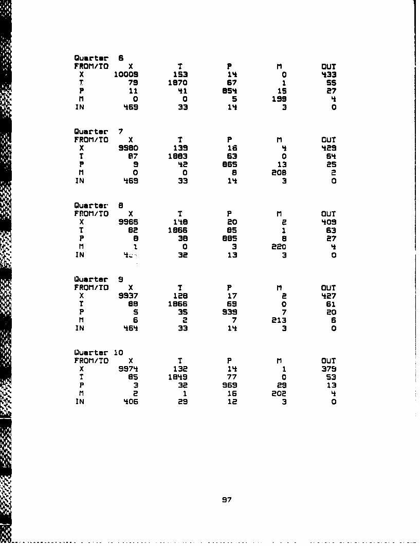
Qumrter 6FROM/TO X T P M OUT
X 10009 153 14 0 433T 79 1870 67 1 55P 11 '1 BS 15 27M 0 0 S 199
IN 469 33 1 3 0
Quarter 7FROM/TO X T P M OUT
X 9580 139 16 ' *29T 87 1863 63 0 64P 9 '2 a65 13 a5M 0 0 a 206 2
IN *69 33 14 3 0
Quarter 6FROM/TO X T P M OUT
X 9965 lie 20 2 409T 82 1666 65 1 63P 8 3B 885 6 27M 1 0 3 220
IN 32 13 3 0
Quarter 9FROM/TO X T P M OUT
X 9937 128 17 2 '27T 6a 1666 69 0 61P s 35 939 7 20m 6 2 7 213 6
IN 464 33 14 3 0
Quarter 10FROM/TO X T P M OUT
X 9974 132 14 1 379T 65 1849 77 0 53P 3 32 569 2s 13M 2 1 16 202
IN '05 29 12 3 0
97

Quarter 11FROM/TO X T P M OUT
X 5856 129 15 1 Li25T 78 1843 72 0 70P 5 39 10.L! 15 18M 2 1 5 212 11
IN 477 34 1 3 0
Quarter 12FROM/TO X T PM OUT
X 9839 169 9 1 440T 93 1843 58 0 52P 7 51 997 17 29M 2 1 10 213 5
IN 474 33 14 3 0
qtr bkord-daus bkord-daWS bkord-max bkord-maxS1 2542031 O.P39700E+08 37 0.539839E+042 10283039 0.103940E+09 135 O.547416E+053 25318113 0.2627S2E÷09 16269 0.874761E+06k 45725105 0.468016E+09 170464 0..180702E+075 55392070 0.65734SE+09 278224 0.432923E+076 72566952 0.80033SE÷09 610511 0.652220E+077 71387379 0.755219E÷05 424163 0.88447E÷078 76820080 0.787362E+09 567692 0.668957E+079 82777372 0.643522E035 663296 0.673289E÷07
10 5606407e 0.5e9930E+09 635084 0.404424E+0711 70996914 0.679970E*09 464729 0.737136E+0712 74435691 0.591572E÷09 672514 0.473270E+17
Average values.5'0591E+08 0.538669E+09 .375260E+06 0.400406E+07
qtr long items long $ commits demval$1 6742 0.341338E+08 0.332l51E+08 0.695378E+082 6810 0.412534E+08 0.209364E+08 0.695906E+083 6890 0.467096E+08 0.3'5610E+08 0.716015E÷08L 69k9 0.504361E÷08 0.236577E+08 0.742740E-085 7014 0.611112E+08 0.382096E+08 0.756709E+086 7083 0.674600E+08 0.240158E+08 0.779703E+087 7207 0.710524E+08 0.371172E+08 0.808892E+08B 7250 0.724052E+08 0.23E827E÷08 0.832453E+089 7358 0.723584E+08 0.353077E+08 0.835426E+08
10 7387 0.881232E+08 0.305129E+08 0.8*0625E+0811 7480 0.927SO7E+08 0.341703E+08 0.860210E-)0812 758' 0.1000i/4E+03 0.311343E+08 0.851144E+OB
Average values7146.2 0.664915E+08 0.305375E+08 0.784517E+08
98
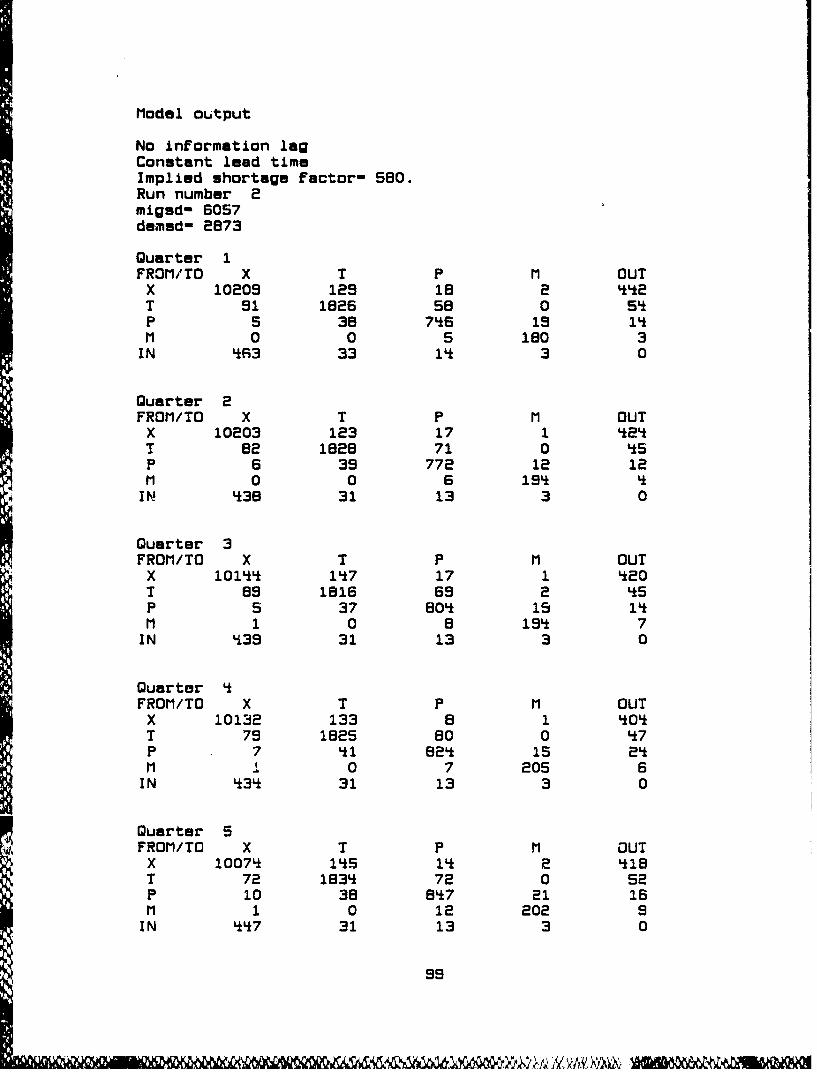
Model output
No information lagConstant lead timeImplied shortage factor- 580.Run number 2migsd- 6057dmsd- 2673
Quarter 1FROM/TO X T P M OUT
X 10209 129 18 2 442T 91 1826 58 0 5P S 38 746 19 14M 0 0 5 180 3
IN 463 33 1* 3 0
Quarter 2FROM/TO X T P M OUT
X 10203 123 17 1 424T 82 1828 71 0 45P 6 39 772 12 12M 0 0 6 194 i
IN 438 31 13 3 0
Quarter 3FROM/TO X T P M OUT
X 10144 147 17 1 420T 89 1816 69 2 45P 5 37 804 15 11*M 1 0 a 194 7
IN L139 31 13 3 0
Quarter LFROM/TO X T P M OUT
X 10132 133 8 1 404T 79 1825 8o 0 *7P 7 '*1 824 1524M 1 0 7 205 6
IN 434 31 13 3 0
Quarter 5FROM/TO X T P M OUT
X 10074 145 14 2 L18T 72 1B34 72 0 52P 10 38 8'*7 21 16M 1 0 12 202 9
IN 447 31 13 3 0
99

Quarter 6FROM/TO X T P M OUT
X 10043 129 22 1 409T 83 1835 71 1 58P 7 s1 BS5 2s 21M 1 0 8 213 6
IN 446 31 13 3 0
Quarter 7FROM/TO X T P M OUT
X 9986 137 14 0 443T 88 1847 68 0 43P 7 37 BOB 17 18M 0 0 6 231 6
IN 461 32 14 3 0
Quarter BFROM/TO X T P M OUT
X 9S5'* 132 19 1 436T 88 18'*5 68 0 52P 12 44 902 is 11M 2 0 6 231 12
IN 464 33 14 3 0
Quarter SFROM/TO X T P M OUTX S943 113 15 2 447T 83 1847 67 0 57P 2 44 926 16 21M 3 1 8 233 9
IN 482 34 14 3 0
Quarter 10FROM/TO X T P M OUTX 9908 143 13 2 447T 103 1829 59 0 Li8P 8 38 940 17 27.M 1 0 9 240 4
IN 474 33 1'* 3 0
100
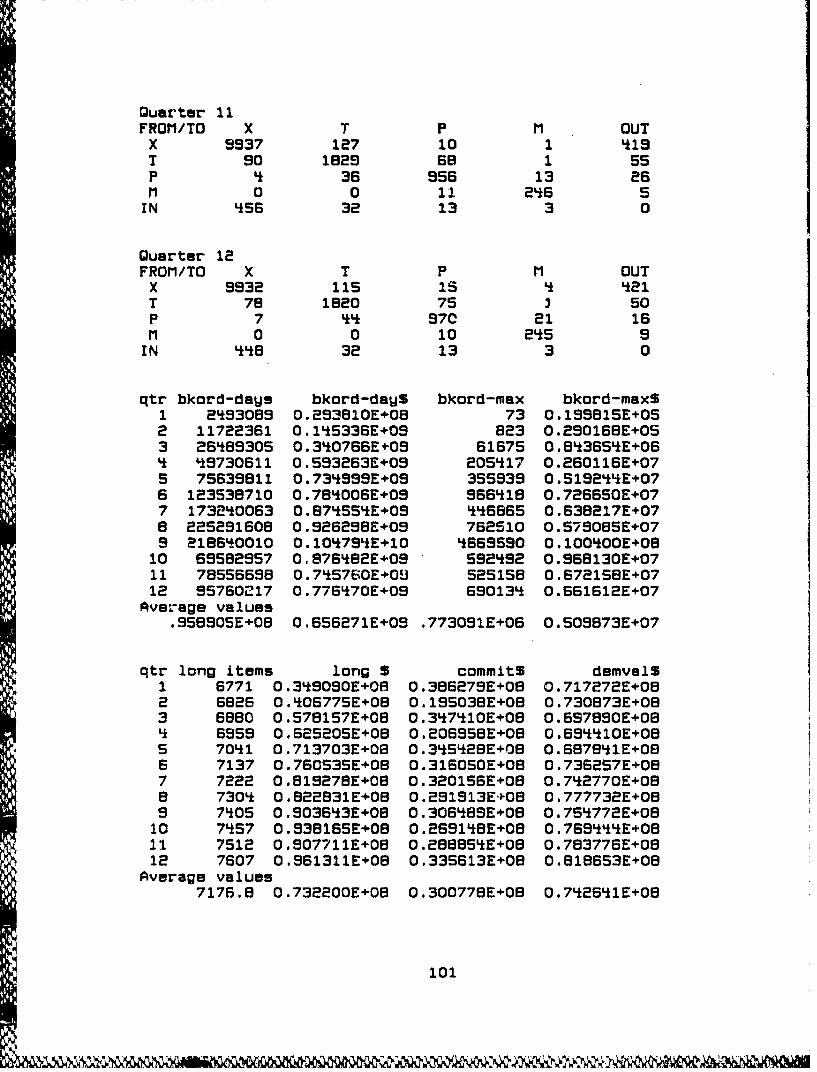
Quarter 11FROM/TO X T P M OUTx 9937 127 10 1 4*19T so 1829 6B 1 55P 36 SS6 13 a6ri a 0 11 2'*6 SIN Lis6 32 13 3 0
Quarter 12FROM/TO X T P M OUTX 9932 115 15 Lt 4*21T 7B 1820 75 3 50P 7 441 97C 21 16fi 0 0 10 24*5 9
IN 44'8 32 13 3 0
qtr bkord-days bkord-dayS bkord-max bkord-maxS1 2'*9308S 0.293810E+08 73 0.199815E4-052 11722361 O.1'*5336E+09 823 0.290168E+053 26'*BS30S O.3'*0766E*'O9 61675 0.84*3654*E+06* '*9730611 O.593253E+O5 205S*17 0.260116E+075 75639811 0.73'*999E+09 355939 0.519244'E+076 123536710 O.78'*006E+09 SSS'*18 0.726650E+077 17324*0063 0.874*554*E+09 44SB665 0.63B217E+078 225291608 0.92629BE+09 762510 O.57S0B5E+079 21864*0010 0.104*794*E+10 4SS669590O.100400OE+0810 69582957 0.s76'*82E+09 552'*2 0.S68130E+0711 78556696 0.74*5760E+09 525158 O.67215BE+0712 SS76O217 0.776'*70E+09 69013'* 0.661612E+07
. SSSOSE080.656271E+03 .773091E+06 O.509873E+07
qtr long items long S commit$ demvalS1 6771 0.34*9090E+08 0.386279E+08 0.717272E+082 6826 0.'*06775E+08 O.195038E+OB 0.730873E4-083 6880 0.578157E+08 0.34*7410E+08 0.E97890E+08
695 0,625.SE205E4-08 O.206958E+08 O.69'*'1OE+085 704*1 0.713703E+08 0.34*5428E+08 0.6878'*1E+086 7137 O.760535E+08 O.316050E+08 O.736257E+087 7222 0.81927BE+08 0.320156E+08 0.7'*2770E+088 7304* 0.822831E+08 0.291913E+08 0.777732E+089 7405S 0.9036'*3E+08 0.3064*89E+08 0.754*772E+0810 74*57 0.9381S5E408 0.2691'*BE+08 0.76S'*'*'E+0811 7512 0.907711E+08 0.28885'*E+08 O.78377SE+0812 7607 0.961311E+08 0.335613E+OB O.818653E+0B
Average values7176.8 0 .732200E+08 0.300778E+08 0.74*26'1E+08
101
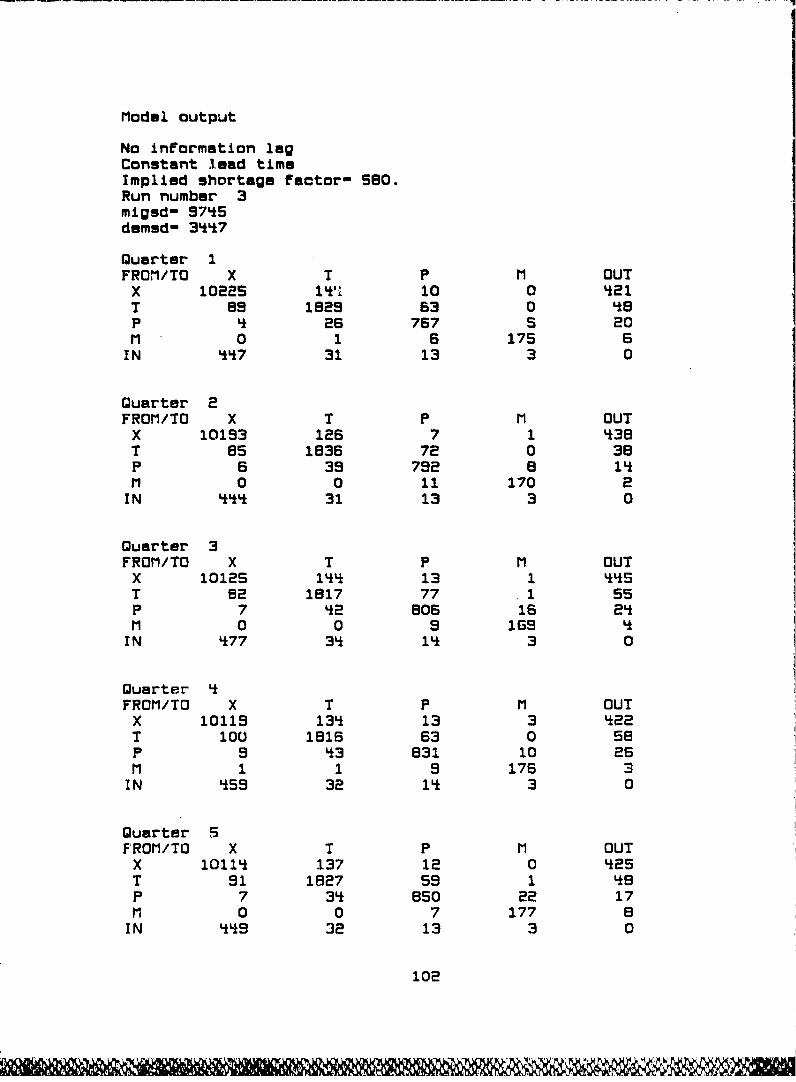
Model output
No information lagConstant lead timeImplied shortage factor- 580.Run number 3migsd- 9745demsd- 3447
Quarter 1FROM/TO X T P M OUT
X 10225 1411 10 0 421T Ps 1826 63 0 L0P 8 2B 767 0 20M 0 1 6 175 6
IN 447 31 13 3 0
Quarter 2FROM/TO X T P M OUT
X 10193 126 7 1 438T 85 1836 72 0 38P 6 38 792 8 14M 0 0 11 170 2
IN 444 31 13 3 0
Quarter 3FROM/TO X T P M OUT
X 10125 144 13 1 5k5T 82 1817 77 1 55P 7 '2 806 16 24M 0 0 9 169 4
IN 477 34 14 3 0
Quarter 4FROM/TO X T P M OUT
X 10119 134 13 3 422T 100 1816 63 0 s8P 9 43 831 10 26M 1 1 9 176 3
IN '*59 32 14 3 0
Quarter 5FROM/TO X T P M OUT
X 10114 137 12 0 425T 91 1827 59 1 418P 7 34 850 22 17M 0 0 7 177 8
IN 449 32 13 3 0
102
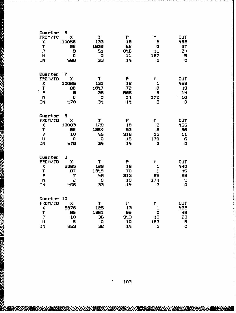
Quarter 6FROM/TO X T P m OUT
X 10056 133 18 a '*52T 92 1639 Be 0 37P 9 51 8'*6 11 2II 0 0 11 187 5
IN '*68 33 1'* 3 0
Quarter 7FROM/TO X T P M OUT
X 10025 131 12 1 LISST 8s 18'*7 72 0 ItsP B 35 885 9 1fI 0 0 ilk 172 10
IN 4*78 34* 1'* 3 0
Quarter 8FROM/TO x T P OUT
X 10003 120 1B 2 4*56T 82 185'* 53 2 56P 10 '*5 918 13 11ii 0 0 16 170 6
IN 4*7B 34* 11 3 0
Quarter SFROM/TO X T P OUT
X 9985 129 18 1 4T 837 18'*9s 70 1 Li6P 7 '*8 913 25S 26
m2 0 10 174 LIN '*66 33 i14 3 0
Quarter 10FROM/TO X T P OUT
X 9976 125 13 1 4*32T 65I 1861 65 0 LisP 10 36 94*3 13 23
m5 0 10 183 6I N Liss 32 14k 3 0
103
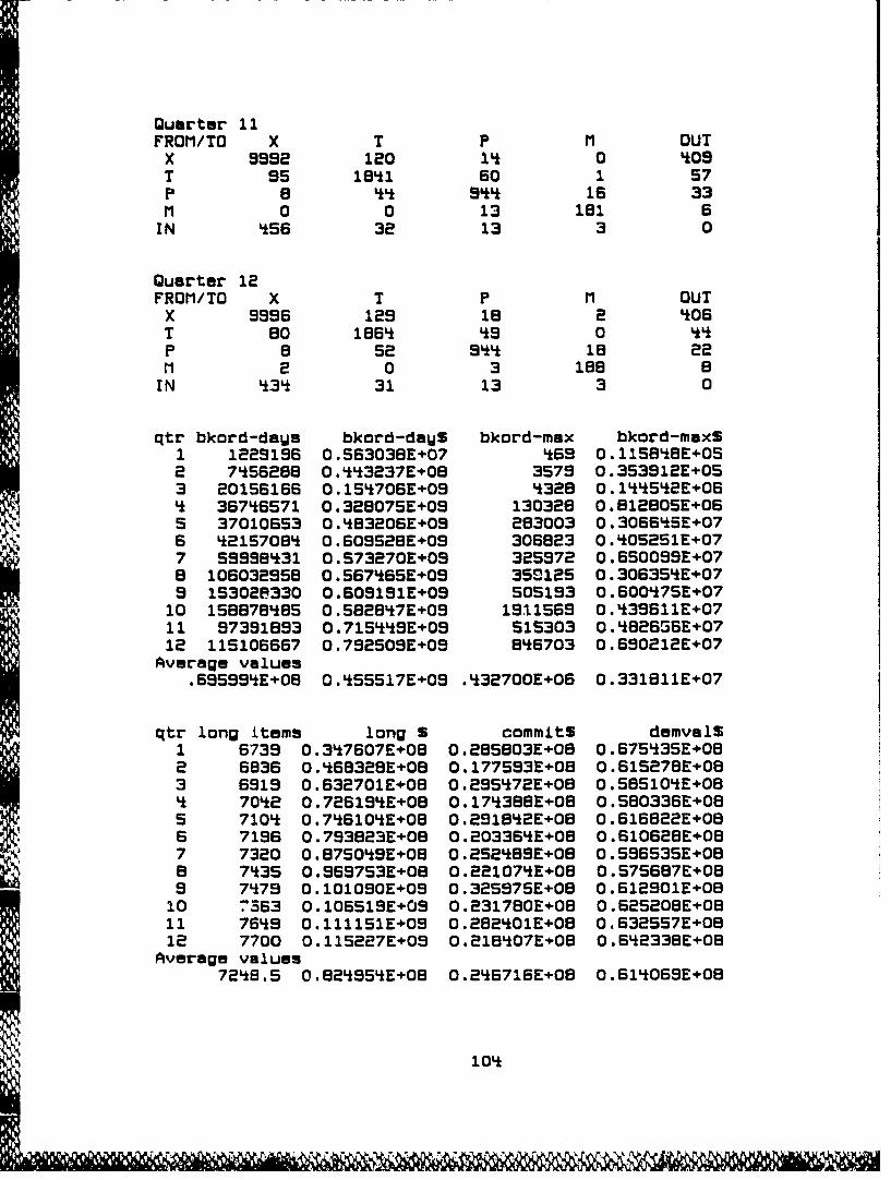
Quarter 11FROM/TO X T P M OUTX 9992 120 14* 0 '*09T 95 184*1 60 1 57P 8 44' 944' i6 33M 0 0 13 l81 6
IN Lis6 32 13 3 0
Quarter 12FROM/TO X T P M OUT
X 9996 129 18 a 4*06T 80 186'* Lis 0 4P a 52 944' lB 22ii 2 0 3 188 BIN 4*34 31 13 3 0
qtr bkord-da~s bicord-daWl bkord-max bkord-maxS1 1229196 0.563038E+07 '*69 O.115B'i8E+OS2 7'*5S288 0.44'3237E+08 3579 0.353912E+053 20156166 0.15'*705E+09 4*328 0.1'*'*5'2E+06'* 367'*6571 0.32807SE+09 130328 0.81280SE+06S 37010653 O.'*83206E+09 283003 0.30566*5E+076 '*21S7084* 0. 60928E409 306523 0.4'*0251Ei-077 599984*31 0.573270E4-09 325972 0.650099E4-078 106032958 0.567'*65E+09 350125 0.30S3S'*E+079 IS3020330 0.S09191E+09 505193 O.600'*75E+07
10 1588784*85 0.5828'*7E+09 1911565 0.4*39611E+0711 97391893 0.7lS44'9E+03 515303 0.'*82SSSE+0712 115106667 0.792509E+09 8'*6703 0.690212E+07
Average values.6S9599'E+08 0 .'55517E+09 .'*32700E+06 0 .331811E+07
qtr long items long S commits damvalS1 6739 0.34*7607E+08 0.285603E+08 0.S75'*35E+082 6836 0.4S08328E+08 0.177593E4-08 0.615278E'083 6919 0.632701E+08 0.295'*72E+08 0.585104*E+08
Lt 704*2 0.725134kE+08 0.174*388E+08 0.580336E+085 7104* 0.74*6104*E+08 0.29184*2E+08 0.616822E+086 7196 0.793823E+08 0.203364*E+08 0.610628E+087 7320 0.8750'*9E+08 0.252'*BSE+08 0.59653SE+OB8 74*3S O.9697S3E+08 0.221074*E+08 0.575687E+089 74*79 0.101090E+09 0.325975E+08 0.612901E+08
10 7363 O.105519E+09 0.231780E+08OB .S25208E+0811 76'*9 0.111151E+09 0.2B2'*01E+05 0.632557E+0812 7700 0.115227E403 0.2184*07E+08 0.64*2338E+08
Average values72t8 .5 0 .e2'95'*E+08 0 .246716E+08 0 .614*065E+08
1'0
1O'*Y
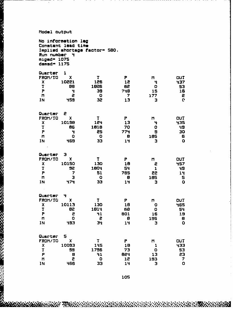
Model output
No information lagConstant lead timeImplied shortage factor- 580.Run number 4migad- 1075demsd- 1175
Quarter 1FROM/TO X T M OUTX 10221 126 12 4 437T 8a 182E 62 0 53P 4 35 748 15 16M 2 0 7 177 2
IN Ls55 32 13 3 0
Quarter 2FROM/TO X T P M OUT
X 10158 124 13 4 435T 85 18i1 70 0 59P 4 25 774 9 30M 0 0 8 185 5
IN Ls65 33 1'* 3 0
Quarter 3FROM/TO X T P M OUT
X 10150 130 18 2 457T 52 1804 5'* 1 49P 7 51 785 22 14M 3 0 8 185 5
IN 474 33 14 3 0
Quarter 4FROM/TO X T P M OUT
X 10113 130 18 0 '*65T 82 1814 68 0 54P 2 41 801 16 19M 0 2 8 155 8
IN 453 34 1'* 3 0
Quarter 5FROM/TO X T P M OUT
X 10053 145 1B 1 433T $5 1756 73 0 53P B '1 824 13 23M 2 0 12 153 7
IN '66 33 14 3 0
105

Quarter 6FROM/TO X T P M OUT
X 10047 134 e5 1 *61T 9' 1801 67 1 S2P 8 37 662 14 20M 0 0 10 194 6
IN 487 34 14 3 0
Quarter 7FROM/TO X T P M OUT
X 10075 144 13 0 L04T 87 1806 6e 0 LI5P 5 '*0 881 .s 27M 2 0 I 204 3
IN 433 29 13 3 0
Quarter BFROM/TO X T P M OUT
X 10001 144 is 3 439
T 80 1828 5s 0 52P 8 37 ass is 30M 1 0 12 211 e
IN 478 34 14 3 0
Quarter 9FROM/TO X T P M OUT
X 997S 143 13 2 435T 77 1851 74 0 41P 8 '3 s68 23 23M 2 0 12 216 6
IN 'S5 32 13 3 0
Quarter 10FROM/TO X T P M OUT
X 9951 137 6 2 '20T 8* 1869 59 0 57P B 51 902 12 27
M 2 0 10 223 9IN '63 33 14 3 0
106
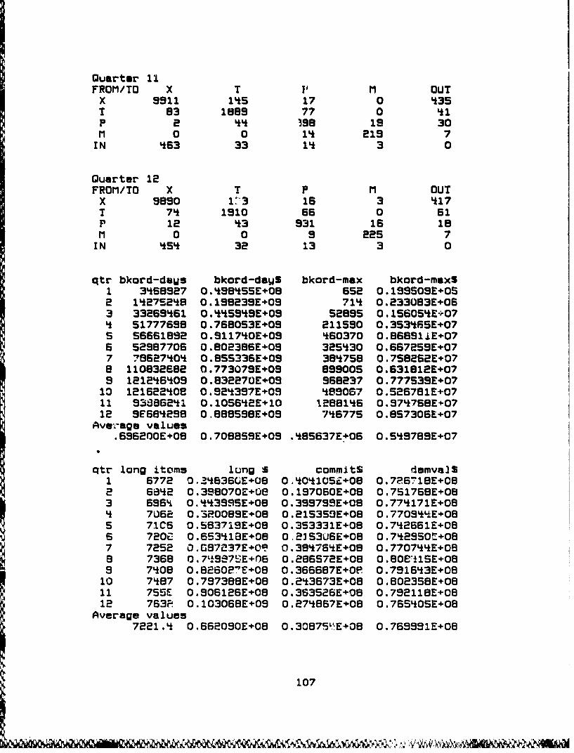
Quarter 11FROM/TO X T M OUTX 5911 1'*5 17 0 4*3ST 83 1es9 77 0 '*1P 2 44' 398 19 30M 0 0 1'* 215 7IN 4S63 33 14* 3 0
Quarter 12FROM/ID X I M OUTX 9890 1 .-3 15 3 4*17T 7'* 1910 65 0 61P 12 '*3 931 16 18II 0 0 9 225 7IN '*5'* 32 13 3 0
qtr bkord-da~s bkord-dauS bkord-max bkord-maxS1 3'*S8927 O.'*98'*SSE+08 552 O.199509E+052 14*2752486 0.198239E+09 714* 0.233083E+063 332S9'*61 O.44'*59'*E+09 52695 015605'*E+O?'* 51777698 O.7S8053E+09 211590 0.3S3'*SSE+075SSSS61892 0.911740OE+09 4*60370 0.8689liE+076 52987706 0.802386E+09 325S430 0.667259E+077 786274*04 0.8S5336E.09 384*7S8 O.7S8262E+078 110832682 0.773079E+09 899005 0.631812E+079 12124S4'09 0.832270E+09 968237 0.777539E.0710 1216224*0E 0.524397E+09 40E9087 0.526781E+0711 933862'*1 0.1056'*2E+1O 12OB1'*6 0.S7'*7SBE+0712 9E58'4298 0.888598E.09 74*6775 0.BS7306L+07
Average values.SS6200E+OB 0.708859E+09 .'*85637E+06 0.5'*9789E+07
qtr long items long 5 commits demvals1 5772 O..43SG36E+O8 O,404O'*1i+08 O.7PS~19E4OB2 S84k2 O.398070E+Ue 0.197060E+08 O.75176BE*083 595Lj O0,44399SE+08 0.399799E+08 0.774*171E+08
4 7062 0.BR00B9E.08 0.215359E+08 O.77094q'E+08S 71CS 0.583719E+08 0.3S3331E+08 O.7'*2S61E4086 720C O.ES3'*18E+08 O,2153USE.08 O.7'*29SO"6+08
7 7252 0.07237E+09 0.384*764E+08 0.770744'E+06B 7368 O.76'SS7SE+06 O.286572E+OB O.Be*15E4-O89 7'*08 0.82602"E+08 O.365587E+0EP 0.7916'*3E+0810 74*87 0.797388E+08 O.2'*3673E*O8 0.802358E+0811 755E 0.506126E+08 O.363526E+08 0.792118E+0812 763F~ O.103068E'-09 0.27'*867E+OB O.765'*OSE+OB
Average values7221.4* 0 .662090E+08 0. 30875ý'E+08 0 .769991E+08
107
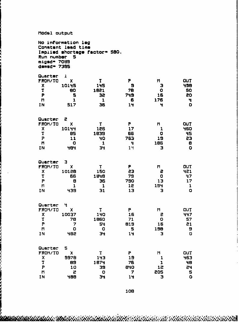
Model output
No information logConstant lead timeImpiled shortage factor- 580.Run number 5migad- 7099demad- 7395
Quarter IFROMI/TO X T P M OUT
X 101'*S 1*5 9 3 498T 80 1821 78 0 50P 5 32 749 16 20M 1 1 6 176
IN 517 36 14 4 0
Quarter 2FROM/TO X T P M OUT
X 10144 126 17 1 '60T 85 1839 66 0 45P 11 40 763 1s 23M 0 1 4 185 8
IN 484 34 1 Lt 3 0
Quarter 3FROM/TO X T P M OUT
X 10128 150 23 2 421T 66 1848 79 0 117P a 36 790 13 17M 1 1 12 195 1
IN 439 31 13 3 0
Quarter 4FROM/TO X T P M OUT
X 10037 140 16 2 447T 78 1860 71 0 57P 7 S' 819 15 21M 0 0 5 IS8 9
IN 482 34 14 3 0
Quarter 5FROM/TO X T P M OUT
X 9978 143 1s 1 463T 85 3.874 76 1 48P 10 39 840 12 24M a 0 7 205 5
IN '88 34 14 3 0
108

Quarter BFROM/TO X T P M OUT
X 9977 155 3 1 431T SB 195 55 1 43P 1e 38 8as 16 81M 0 1 11 207 3
IN *9S 32 13 3 0
Quarter 7FROM/TO X T P M OUT
X 99'6 118 16 a '50T 93 1912 60 1 Li5P 6 to0 878 1 a5M 1 1 6 212 e
IN '77 34 14 3 0
Quarter 8FROM/TO X T P M OUT
X 9902 141 16 8 '62T 87 1893 6o 1 64P 11 44 881 14 20M 3 0 9 213 5
IN 498 34 14 4 0
Quarter 9FROM/TO X T P M OUT
x 9905 136 12 1 447T 95 1902 65 1 50P 9 33 age is 25M 1 0 4 22S 10
IN 481 34 14 3 0
Quarter 10FROM/TO X T P M OUT
X 9899 119 a 1 463T B2 1900 63 1 59P 9 40 315 a 15M 0 0 10 230 5
IN *92 34 14 3 0
109
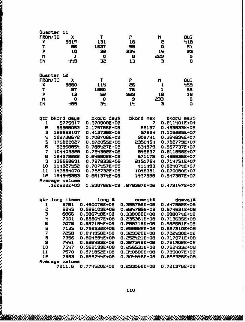
Quarter 11FROM/TO X T P M OUTX 991'5 131 15 2 Li18T 96 1837 59 0 51P 10 32. 93LA 23M 1. 0 8 229 5IN 44'9 3e 13 3 0
Quarter 12FROM/TO X T P M OUTX 9860 uis 26 1 LISST 97 1860 76 1 58P 13 52 929 18 18M 0 0 9 233 5IN *89 34* 14 3 0
qtr bkord-da~s bko&'d-daWS bkord-mmx bkorr.;-maxS1 9775517 O.370S08E*08 7 0.2114i01E+04*2 55368053 0.17S786E+09 2e137 0.Li33833L4053 129959107 0.4*13738E+09 S7694i O.l0522SEe07Lj 198738572 0.708706E+09 90874i1 0.36Li69LE'07S 175822027 0.872055E4-09 2350Li5L 0.782779E+076 9286885Li 0.7884i27E+09 S34i979 O.657737E+077 1044~03928 O.72Li382E.09 9LiS837 0.81185SE+078 124i3792B2 O.6Li5802E+09 571175 O.Li5663SE+079 135668691 0.727833E+09 e15176Li 0.71Li7S1E+07
10 11Li827LiS2 0.7O7Li57E+OS 4i114i93 0.S2'107'*E+0711 1Li368Li070 0.722732E4-09 10486381 O.S70080E1.0712 18Li8LiS53 O.66137'*E+09 14*37988 0.5Li7387E+-O7
Average values.122529E+09 0.598782E+09 .878387E+06 0.4i7914i7E+07
qtr long items long S commits demvalS1 6781 O.Li60076E+CB 0.355755E.08 0.6'*7982E+082 S8'*S O.S25109Ee08 0.22'*78SE+08 0.67Li631E+083 6866 O.S867Li8E+08 0.338086E+08 O.58907'*E+08Li 7001 0.6580Li7E+08 0.23S361E+OB 0.713S35E.085 7076 O.69718LiE*08 0.29871SE+08 0.582691E+086 7135 0.798532E+08 0.258822E+08 0.687910E4-087 7258 O.8Li4958Ee08 0.329328E+08 0.7224i90E+088 7356 0.9Oi29LiE+CB 0.2S2Li21E.08 O.717971E+089 744~1 0.9284i93E+08 0.32734i2E+08 O.7513O2E+O810 754i7 0.962199E+08 0.2S6S31E+O8 0.7S2Li93E4-08p11 7570 O.971852E+08 0.3Li0680E+08 0.795O07E+O812 7663 0.556744~E+08 0.30494L6E+08 0.822326E+08
Average values
7211.5 0 .77Li520E+08 0 .293568E+08 0 .72137SE+08I 110
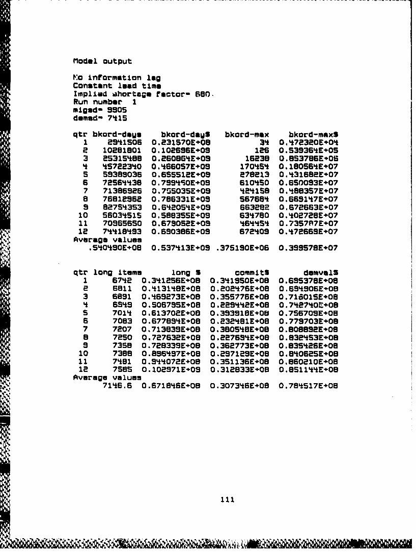
Model output
V:o information lagConstant lead timeImplied ahorta;m factor- 680.Run number 1migud- 9505demad- 7415
qtr bkord-days bkord-day$ bkord-max bkord-maxS1 2941505 0.231570E÷08 34 0.472320E÷042 10281801 0.102696E÷09 125 0.539354E÷053 25315*89 0.260854E÷05 15238 0.853786E+064 45722340 0.*66057E+09 170454 0.18056'E+07S 59385035 0.655512E÷09 278213 0.431682E÷075 7256S438 0.7951*0E+09 610450 0.650093E+077 71386926 0.7S5O35E+09 424158 0.488357E5078 76812952 0.785331E÷09 55768* 0.569147E5079 82754353 0.642O54E+09 663282 0.672663E+07
10 56034515 0.588355E+09 634780 0.402728E+0711 70SS5650 0.679052E+09 46454 0.7357P7E÷0712 74418493 0.690386E+09 S72409 0.472669E+07
Average values.540490E+08 0.537413E+09 .375190E+06 0.399578E÷07
qtr long items long S commits domvalS1 6742 0.341 256E÷08 0.341950E+08 0.695378E÷082 5811 0.413148E+08 0.202476E+08 0.699065E+083 6891 0.469273E÷08 0.355776E÷08 0.716015E+08
5 699 0.506755E+08 0.229542E+08 0.742740E+08S 7014 0.613702E+08 0.393918E+08 0.758709E÷086 7083 0.677854E÷08 0.232481E+08 0.775703E5087 7207 0.713839E÷08 0.380548E+08 0.808892E÷088 7250 0.727632E+08 0.227694E+08 0.832453E+089 7358 0.7283395E08 0.362773E+08 0.8354265E+08
10 7388 0.896497E+08 0.297129E÷08 0.840525E÷0811 7481 0.944072E+08 0.351136E+08 0.860210E÷0812 7585 0.102971E+09 0.312833E+08 0.8S111*E÷08
Average values7146.6 0.671846E÷08 0.307346E+08 0.784517E÷08
S~111
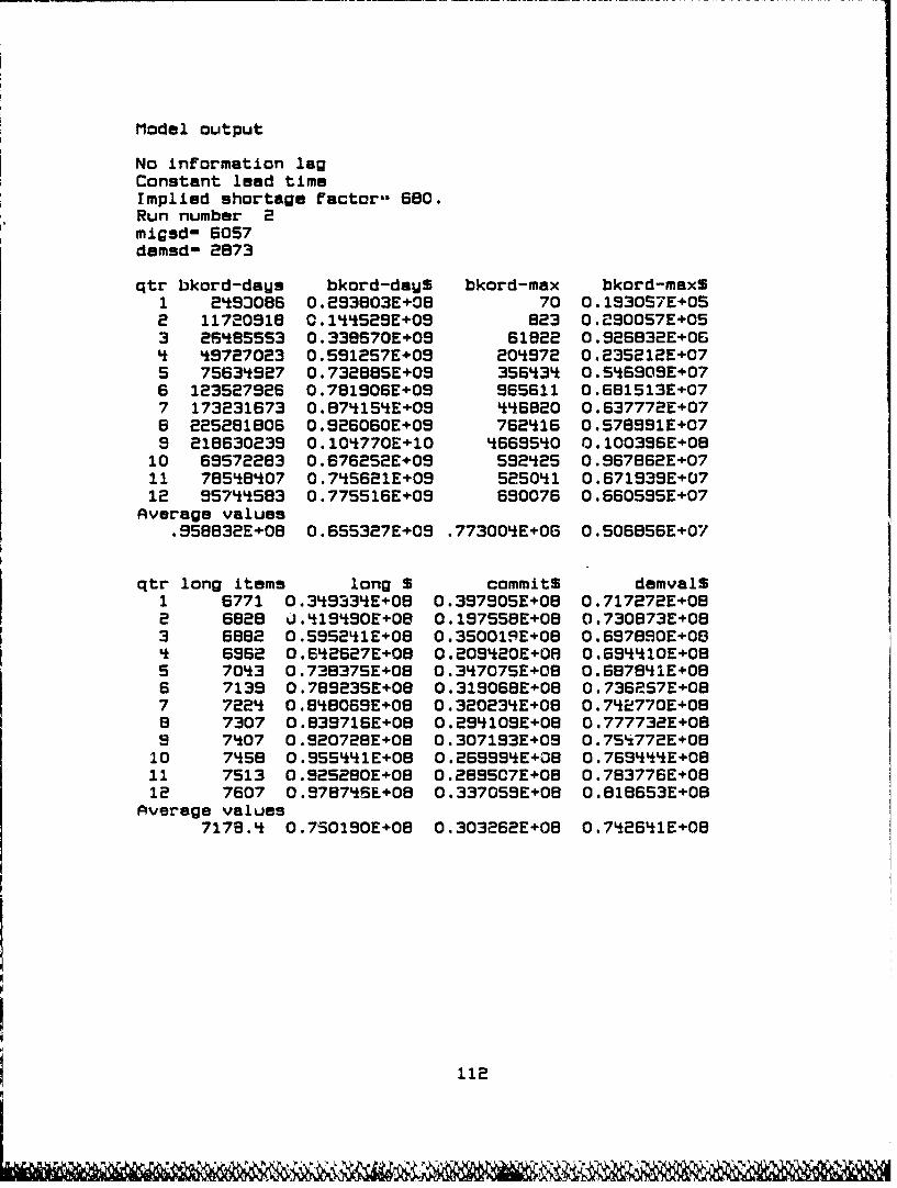
Model output
No information lagConstant lead timeImplied shortage factor" 680.Run number 2migad- 6057dumsd- 2873
qtr bkord-days bkord-dayS bkord-max bkord-maxS1 2493086 O.293803E+08 70 0.1930S7E+052 11720918 0.144529E+09 823 0.290057E+053 265855S3 0.338S70E+09 61822 0.925B32E+064 49727023 0.591257E+09 204972 0.235212E+075 75634927 0.73288SE+09 356134 0.546909E÷076 123527926 0.781906E+09 965611 0.681513E+077 173231673 0.874l15E+09 4B6B20 0.637772E+075 225281806 0.926060E+09 762416 0.578991E+079 218630239 0.104770E+10 4669540 0.100396E+08
10 69572283 0.676252E+09 592425 0.967862E+0711 78548407 0.745621E+09 525041 0.671939E+0712 957iSO83 0.77SS16E+09 690076 0.660S9SE+07
Average values.958832E+08 0.655327E+09 .773004E+06 0.506856E+07
qtr long items long S commits demvalS1 6771 0.349334E+08 0.397905E+08 0.717272E+082 6828 0.419490E+08 0.197558E+08 0.730873E+083 6882 0.59SS21E+08 0.3S0019E+08 0.697890E+08Lt 6962 0.652627E+08 0.2OS20E+0B 0.58L410E+085 7043 0.73837SE+08 0.347075E+08 0.687841E+086 7139 0.789235E÷08 0.319068E+08 0.7362S7E+087 7224 0.8i8069E+08 0.320234E+OB 0.742770E+088 7307 0.839716E+08 0.294109E+08 0.777732E+089 7407 0.920728E+08 0.307193E+03 0.75'z772E+08
10 7458 0.955441E+OB 0.259994E+08 0.769444E+0811 7513 0.92S280E÷08 0.2895C7E+08 0.783776E+0812 7607 0.97876SE÷08 0.337059E+08 0.818653E+08
Average values7178.4 0.750190E÷08 0.303262E+08 0.742641E+08
112
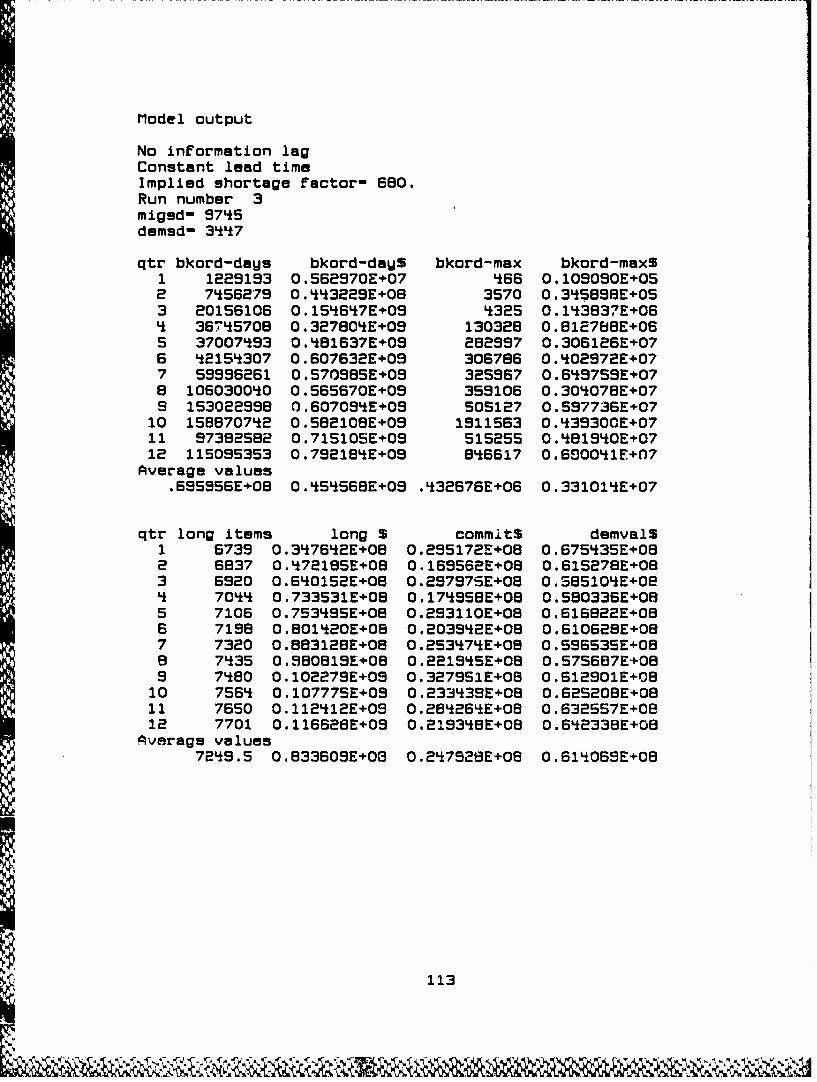
Model output
No information lagConstant lead timeImplied shortage factor- 680.Run number 3migsd- 9745demsd- 3447
qtr bkord-days bkord-daUS bkord-max bkord-maxS1 1229193 0.562970E+07 466 0.109090E+052 7k56279 0.443229E+08 3570 0.345898E+053 20156106 0.1546k7E+09 4325 0.1'*3837E+064 36745708 0.327800E+09 130328 0.812788E+06S 37007493 0.481637E+09 262997 0.306126E+076 42154307 0.607632E+09 306786 0.402972E+077 59996261 0.570985E÷09 325567 0.659759E+078 106030040 0.565670E+09 359106 0.304078E÷079 153022998 0.607094E+09 505127 0.597736E+07
10 15B870742 0.582108E+09 1911563 0.439300E+0711 97382582 0.71510SE÷09 515255 0.l8194OE+0712 115095353 0.792184E+09 846617 0.690041E+07
Average values.695956E+08 0.555568E+03 .432676E+06 0.331014E+07
qtr long items long S commits demvalS1 6739 0.376542E+08 0.295172E+08 0.675535E+OB2 6837 0.472185E+08 0.169562E+08 0.615278E+083 6920 0.6i0152E+08 0.297975E+0B 0.8S51I0E+094 7044 0.733531E+08 0.174958E+08 0.580336E+085 7106 0 .753495E+08 0.293110E+08 0.616822E+086 7198 0.801420E+08 0.203952E+08 0.610628E+087 7320 0.883128E+08 0.253474E+08 0.596535E+08B 7435 0.980819E+08 0.221955E+OB 0.575687E+089 7480 0.102279E+09 0.327951E+08 0.612901E+08
10 756' 0.107775E+09 0.233439E+08 0.62S208E+0811 7650 0.112412E+09 0.284264E+08 0.632557E+0812 7701 0.116628E+09 0.219348E+08 0.642338E+08
Average values7259.5 0.833609E+08 0.247928E+08 0.614069E+08
113
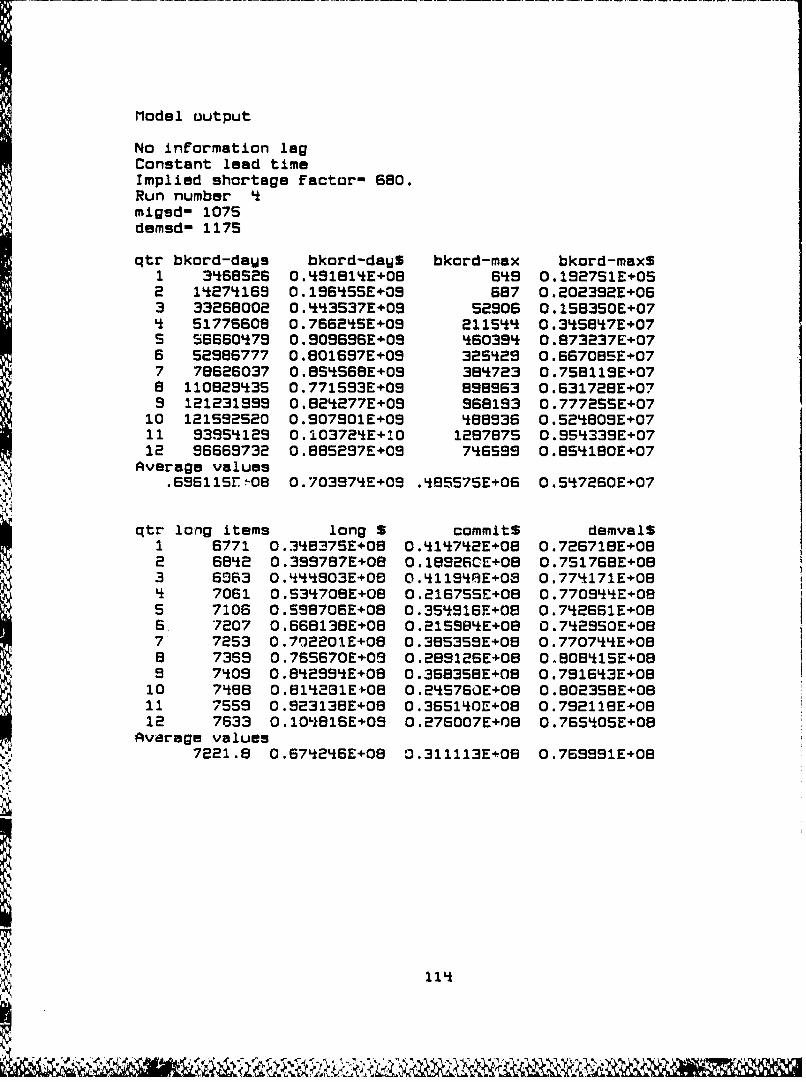
Model output
No information lagConstant lead timeImplied shortage factor- 680.Run number k
migsd- 1075demsd- 1175
qtr bkord-daUs bkord-dayS bkord-max bkord-maxS1 3'58526 0.491814E+08 649 0.192751E+O52 14274169 0.196*55E+09 687 0.202392E+o63 33268002 0.453537E+09 S2906 0.1S8350E+07* 51776608 0.766245E+09 2115S4 0.36SB17E+07S 56660479 0.909696E*09 460394 0.873237E+076 52986777 0.801697E+09 325429 0.667085E+077 78626037 0.85*568E+09 384723 0.758119E+078 110823435 0.771593E+09 898563 0.631728E+079 121231999 0.825277E+09 968193 0.7772SSE+07
10 121592520 0.907901E+09 488936 O.521809E+0711 9395129 0.103724E+10 1287875 0.954339E÷0712 96669732 O.885297E+09 746599 0.854180E+07
Average values.6961151E08 0.703974E+09 .486575E+06 0.547260E+07
qtr long items long S commits demvalS1 6771 0.34837SE+08 0.41712E+08 0.726718E+082 6862 0.399787E+08 0.18926CE+08 0.7S1768E+083 6363 0.444803E+08 0.411940E+08 0.774171E+084 7061 0.534708E+08 0.216756E+08 0.770944E+085 7106 0.598706E+08 0.356916E+08 0.742661E+086. 7207 0.668138E+08 0.21S981E+08 0.7529S0E+087 7253 0.702201E+08 0.385359E+08 0.770744E+088 7369 0.765670E+09 0.289126E+08 0.808'15E+089 7409 0.842994E+08 0.368358E+08 0.791643E+08
10 7488 0.814231E+08 0.245760E+08 0.802358E+0811 7559 0.923138E+08 0.365140E+08 0.792118E+0812 7633 0.10*816E+09 0.276007E+08 0.765S05E+08
Average values7221.8 0.674246E+08 0.311113E+08 0.769991E+08
114

Model output
No information lagConstant lead timeImplied shortage factor- 680.Run number 5migsd- 7095demsd- 7395
qtr bkord-daUs bkord-daWS bkord-max bkord-max$1 977569' 0,367283E008 4 0.143822E+042 S5367771 0.175336E+09 22128 0.425782E+053 129958608 6.412868E+09 57678 0.102801E÷074 198737953 0.707570E+09 908805 0.377641E+075 175619199 0.870072E+09 2350279 0.751974E+076 92863351 0.787103E+09 635176 0.697873E+077 104391072 0.721593E+09 945795 0.810875E+07B 124355263 0.653301E+09 571073 0.466521E+079 135644804 0.725690E+09 21Sl50L 0.710890E+07
10 118036B7 0.704913E+09 411376 0.61973BE÷0711 143636680 0.720249E÷09 1047869 0.6734 25E+0712 164799077 0.659142E+09 1437881 0.540151E+07
Average values.122514E+09 0.596965E+09 .878297E÷06 0.479691E+07
qtr long items long S commits demvalS1 6780 0.464074E+08 0.366944E+08 0.647982E+082 6845 0.52958BE+08 0.219140E+0B 0,674631E+083 6866 0.595050E+08 0.347689E+08 0.688074E+084 7001 0.666647E+08 0.228020E+08 0.713635E+08S 7076 0.739376E+08 0.307321E÷08 0.682691E+086 7135 0.810865E+08 0.251974E+01 0.687910E+0O7 7258 0.857876E+08 0.338824E+08 0.722490E+088 7356 0.917574E+08 0.246486E+08 0.717971E+089 7440 0.941850E+08 0.336074E+08 0.751302E+08
10 7546 0.975SB5E+08 0.258581E+08 0.752493E+0811 7570 0.984991E+08 0.350479E+08 0.755007E+0812 7662 0.971422E+08 0.293081E+08 0.822326E+08
Average values7211.3 0.785405E+08 0.295052E+08 0.721376E+08
115

Model output
No information lagVariable lead timeImplied shortage factor- 580.Run number 1migsd- 390Sdamsd- 741S
qtr bkord-days bkord-daUS bkord-max bkord-max$1 2942031 0.239700E+08 37 O.S39899E+0O2 10283039 0.103940E+09 135 0.547416E+053 25318113 0.262752E+09 16269 0.874761E÷064 491377354 0.494541E+09 24246 0.82OSSE+06S 78372400 0.816086E+09 2S8955 0.304403E+076 99083954 0.115849E+10 373424 0.5L5921E+077 119150158 0.126654E÷10 738993 0.703028E+078 118359093 0.1302869E+10 775766 0.653267E+079 121434913 0.133768E+10 577076 0.728852E+07
10 145295152 0.136568E+10 692613 0.926055E+0711 147241451 0.108064E+10 969165 0.616925E+0712 111959371 0.124032E+10 507054 0.8652032E+07
Average values.857856E÷08 0.871127E+09 .411977E÷06 0.459348E+07
qtr long items long S commits demvalS1 6743 0.34EO2IE608 0.350687E÷08 0.655378E+082 6612 0.415778E+08 0.22B816E+08 0.695906E+083 6891 0.472189E+08 0.368807E+08 0.716015E+0B4 6951 0.S11395E+08 0.259376E+0B 0.742740E+085 7014 0.625293E+08 0.418076E+08 0.756709E+086 7085 0.69S239E÷08 0.260334E+08 0.779703E÷087 7209 0.732558E+08 0.395035E÷08 0.808892E+088 7252 0.749899E+08 0.251683E+08 0.8324S3E÷089 7357 C.761031E+08 0.371411E+08 0.835426E+08
10 7386 0.928366E+08 0.34&248E÷08 0.84062SE+0811 7487 0.982588E+08 0.354157E+08 0.860210E+0812 7588 0.106077E+09 0.342710E+08 0.8511½kE+08
Average values7147.9 0.689771E+08 0.329612E+08 0.786517E+08
116

Model output
No information lagVariable lead timeImplied shortage factor- 580.Run number 2migsd- 6057dearnd- 2873
qtr bkord-da~s bkord-daUS bkord--max bkord-maxS1 24k93089 0.293810E+08 73 O.19561SE+O52 11722361 0.1'*533SE+05 823 0.250168E'053 26'*89305 0.3'*07SSE+O9 61E75 0.8Lk365LE4.06Li 54890459S 0.518204kE+09 27551 0.171028E+075 5L*S344945 0.880625E-09 383610 0.E56767E+076 14*8733SSS 0.12244~1E+10 1036308 0.517608E+077 208Lk55657 O.125155E+1O 37131B 0.S52683E+078 266150095 0.1324102E+10 765227 0.738985E*075 3233931&*S 0.1Li5651E+10 2&*7L0SS 0.79S799E+07
10 382028137 0. 175910E+10 3338074* 0. 1044~56E+OB11 182211B8i0 0.165552E+10 lOSS0LIS 0.130268E+0B12 158198161 0.12S51LiE+10 1056886 0.601916E+07
Average values.155112E+09 0.100181E+10 .8B't39lE+O6 0.5Li7652E+07
qtr long items long S commit$ demvalS1 6770 0.349S480E+08 0.4*12019E4+08 0.717272E+082 6626 0.L10787SE+08 0.2111S8E+08 0.730873E+083 6881 0.5B6535E+0B 0.373121E+08 0.657890E+08
It 6562 0.635Li01E4-08 0.224i558E+08 0.S5Li410E+0B5 7044~ 0.731233E+08 0.376363E+08 0.S878Li1E4086 7137 0.781631E+08 0.357665E+08 0.7362S'7E+067 7224i 0.84*085L4E+08 0.3Li0102E+08 0.74i2770E+08a 7307 0.B50Li77E+08 0.3244~05E+08 0.777732E+08a 74i05 0.536Li4i4E+0B 0.330709E+0B 0.75.L'772E+OB
410 7Li61 0.97Li2S3E+08 0.290392E+08 0.765Li4i4E+0811 7520 0.5L46733E+08 0.310573E+08 0.783776E+0B12 7613 0.100875E+09 0.3682'*3E+08 0.818653E*OB
Average values7175.2 0.754i144LE+08O 0.326651E+08 0.74i26Li1E+08
117

Model output
No information legVariable lead timeimplied shortage factor- 580.Run number 3migad- 974*5doemd- 344'7
qtr bkord-da~s bkord-daUS bkord-max bkord-maxS1 1229196 0.563038E+07 '*69 0.1156'*BE+OS2 7'*56268 0.44'3237E+08 3579 0.353912E+053 20156166 0.1S'*706E+0S '328 0.1'*'*5'2E+06Lt 306S110'* 0.336631E+09 '*356 0.35197SE+06S 51223163 O.560551E+09 4*1014*9 0.312532E+076 SS044'313 0.787810E+09 1ES227 0.34*7413E+077 55316153 0.975958E+O9 3S704*7 0.'*60'*6E4-078 135705110 0.109107E+10 '*65280 0.7'*7032E+079 177751377 0.B66871E+09 4*25885 O.'*06O4'E+O7
10 24S594304*7 0.102090E+10 627535 0.5528'kSE+0711 307560151 0.107364kE+10 810753 0.630771E+0712 34*91S0030 0.12194*1E+10 2516368 0.500511E407
Average values.123301E+09 O.678'*9E+O5 .5lS27SE+06 0.34*2697E+07
qtr long items long S commits demvalS1 6735 0.3'i5057E+08 0.25323BE+08 0.675'*35E+082 6834* 0.4*69832E+08 o.le9507E+OB 0.615278E+083 5520 0.635299E+08 0.32062'*E+08 0.58510'*E4081* 704*0 0.725581E+05 0.18S065E~08 0.S60336E+085 7102 0.7512B6E+08 0.313902E4-08 0.61BB22E+086 7197 0.806533E.0B 0.223BB6E.08 o.s1062eE+0B7 7321 0.e9'*988E+08 0.257'k52E+08 0.556535E+06a 7'*3S 0.10049S1E4-09 0.2'*'665E+06 0.57SSB7E+D89 74*7S 0.105577E+09 0.367255E+08 0.612901E4-0810 7561* 0.11219'*E+09 0.253006E+08 0.62S206E+0811 7652 0.117014*E+03 0.311650E+08 0.63ES57E+0812 7703 0.1220S4*E+09 0.24*'376E+08 0.6'*2338E+08
Average values724e8.8 0 .850781E+08 0 .268239E+08 0 .61'*069E+08
-li
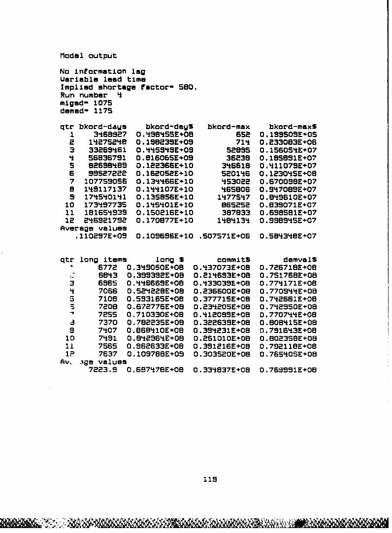
Model output
No information lagVariable lead timeImplied shortage factor- 580.Run number 4migsd- 1075demud- 1175
qtr bkord-daus bkord-daWS bkord-max bkord-maxS1 3468927 0.498455E+08 652 0.195509E+052 1427524B 0.158239E+09 714 0.233083E+063 33269461 0.445949E+09 52895 0.15605'E+074 56836791 0.816065E÷09 36238 0.185891E+07S 82S98489 0.122366E+10 34S618 0.k1107SE+07S 99527222 0.162052E÷10 520146 0.1230LSE+087 107759056 0.1344S6E610 453022 0.670098E+078 149117137 0.144107E+10 465806 0.947089E+079 174540141 0.135856E+10 1477547 0.8*9610E+07
10 173497735 0.145401E+10 865252 0.839071E+0711 181654939 0.10216E+10 387833 0.698S81E+0712 2S6921792 0.170877E+10 148413q 0.998945E+07
Average values.110297E+09 0.109696E+10 .507S71E+06 0.58*348E+07
qtr long items long S commits demvalS6772 0.349050÷E08 0.437073E+08 0.726718E+0856843 0.399392E+0B 0.214693E+08 0.751768E+08
3 6965 0.'*6669E+08 0.433039E+08 0.774171E+08S7066 0.S24228E÷08 0.236600E+08 0.770944E+085 7108 0.593165E+08 0.377715E+08 0.742661E+08
7208 0.672776E+08 0.234205E+08 0.742950E+087255 0.710330E+08 0.412099E+08 0.770744E+08
a 7370 0.782235E÷08 0.322639E+08 0.808415E+089 7407 0.668410E+08 0.394231E+08 0.7916*3E+08
10 7491 0.8429S6E+08 0.261010E+08 0.802356E+0811 7565 0.S62633E+08 0.391216E+08 0.792118E+081P 7637 0.109788E+09 0.303520E+08 0.7650*SE+08
Av ,Age values7223.9 0.687478E+08 0.334837E+08 0.769931E+08
119
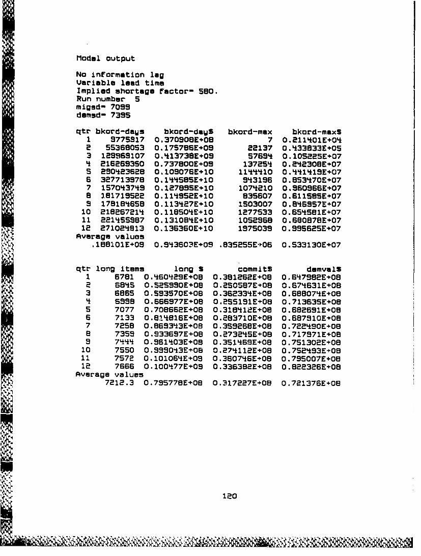
Model output
No information logVariable lead timeImplied shortage factor- Sea.Run number Smigsd- 7099demsd- 7395
qtr bkord-daus bkard-daWS bkord-max bkorcl-max$1 9775917 0.370508E.06 7 0.211Lk01E04O~2 55368053 0.175766E.09 22137 0.'*33B33E+053 129965107 0.4*13738E+09 5755'* 0.105225E+07'* 216269350 0.737800E+09 1372S4* 0.24k2308E+07S 2904*23628 0.105076E+10 11444*~10 0.4*1'*19E+076 327713576 0.144585E+10 9'i319S 0.BS3'*70E+077 1S704i3749 0.127895E+10 1074k210 0.SSO965E+078 3.81719S22 0.114t552E+10 635507 0.611585E+079 17B16'k656 0.113427E+10 1503007 0.6'*6557E+07
10 2182S7214 0.118504*E+10 1277533 0.65'*561E+0711 221Lk5SS87 0. 13108'*E+10 1052556 0 .660878E+0712 2710248613 0. 13S630E+10 1975035 0 .995625E+07
Average values.1B6101E+05 0 .9'43S0E+09 .83525SE-106 0 .533130E+07
qtr long items long S commit$ demvalS66S71 0.452590E408 0.381252E+08 0.64716311+0
67617 0.7086'25E+08 0.318412E+08 0.5'*752E4-06
6 7330.811616E+0B 0.283710E+08 0.687910E+087 7258 0.BS53Lk3E+08 0.3S9268E+06 0.722&*90E+086 735S 0.933657E+08 0.2732'*5E+06 0.717571E+089 711'4 0.SS1103E+08 0.351'*6.E+08 0.751302E+08
10 7550 0.S999O-3E+08 0.274*112E+08 0.752493E+0811 7S72 0.10106'*E+0S 0.3607'*6E+06 0.795007E.OB12 7666 0.100'*77E+05 0.336362E+08 0.822326E+08
Average values7212.3 0 .795778E+08 0.317227E+08 0.721376E+08
120

Model output
No information lagVariable lead timeImplied shortage factor- 580.Run number 1migsd- 9905demed- 7415
qtr bknrd-daWs bkord-daWS bkord-mmx bkord-maxS1 294150S 0.231570E+08 34 0.472320E+042 10281801 0.102696E÷09 126 0.53936S+0S3 25315488 0.26086'E+09 15238 0.853786E+064 4997S6B5 0.492683E÷09 24236 0.880672E+065 78369503 0.814095£+09 266941 0.30*22SE+076 99080394 0.11S650÷E10 373366 0.543752E÷077 119147079 0.126533E+10 738960 0.701919E+078 118361920 0.130217E÷10 775756 0.653445E+079 121411278 0.133617E+10 577009 0.723168E+07
10 155285234 0.135381E+10 692377 0.924371E+0711 147202138 0.107B39E÷10 969055 O.616392E+0712 111916575 0.123781E+10 510341 0.B5128BE+07
Average values857723E+08 0.869473E+09 .412205E+06 0. *58573E+07
qtr long items long S commits demvelS1 6743 0.341962E+08 0.360536E+08 0.695378E.082 Se13 0.41S'•E6+08 C.22220oE+k.9 0.69'906E+063 6S92 0.474482E+06 0.379372E+08 0.71601SE+OBS6951 0.S13921E÷08 0.252331E÷06 0.742700E+085 7014 0.629117E+08 0.430719E+08 0.756709E+086 7085 0.697870E+08 0.252888E+08 0.779703E+087 7205 0.736200E+08 0.404979E+08 0.808892E+08a 7251 0.753943E+08 0.243646E+08 0.832453E+089 7357 0.766593E+08 0.381370E+08 0.835426E+0810 7367 0.94*5818E08 0.336666E+08 0.B40625E+0811 7488 0.100010E+09 0.373956E+08 0.860210E+0812 75689 0.109096E+09 0.344386E+08 0.85114*E+08
Average values714B.3 0.697162E+08 0.331971E+08 0.78517E+08
121
I2
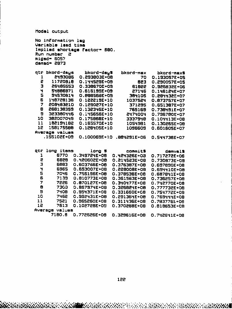
Model output
No information lagVariable lead timeImplied shortage factor- 660.Run number 2migod- 6057demmd- 2873
qtr bkord-daWs bkord-deWS bkord-max bkord-maxS1 2593086 0.293803E÷08 70 0.193057E+0S2 117208ie 0.145529E+09 8e3 0.290057E+053 26485S53 0.338670E+09 61822 0.926832E÷06S5S4886871 0.616199E÷09 271S6 0.156124E+07S 95530814 0.88856BES09 38410S 0.284432E+076 148726136 0,122219E+10 1037S24 0.8737S7E÷077 208483210 0.12S027E+10 371295 0.651387E÷076 268138355 0.132346E÷10 765169 0.738591E+079 323380446 0.145656E÷10 2474004 0.796780E÷07
10 382007059 0.175668E+10 3337958 0.104413E+0811 182195182 0.165S70E+10 lOS10 81 0.13026SE÷0B12 .58175588 0.128405E+10 1095609 0.601605E+07
Average valuesS155102E+09 0.100069E+10 .884291E+06 0.544738E÷07
qtr long items long S commits demvalS1 6770 0.359724E+08 0.424326E+08 0.717272E+062 682B 0.420602E+08 0.214S23E+06 0.730873E+083 6883 0.603766E+08 0.376387E+08 0.697830E+08Lt 6955 0.653007E+08 0.228008E+08 0.694410E+08S 7056 0.756196E+08 0.376536E+08 0.687841E+086 7139 0.810773E÷08 0.361563E+08 0.736257E+087 7226 0.870127E+06 0.340477E+08 0.742770E+088 7303 0.867974E+08 0.326824E+08 0.777732E+089 7408 0.955371E+08 0.331660E+0B 0.754772E+06
10 7562 0.352431E+08 0.291365E+08 0.769444E+0811 7521 0.965260E+08 0.311436E+08 0.783776L+0812 7613 0.10272BE+0S 0.37028BE+06 0.8186S3E+CB
Average values7180.8 0.772626E÷08 0.329616E+08 0.742641E+08
122

Model output
No information lagVariable lead timeImplied shortage factor- 680.Run number 3migad- 5745dmmsd- 3447
qtr bkord-daUS bkord-dauS bkord-max bkord-maxS1 1229193 0.5629706E07 465 0.109090E+052 7i56279 0.443eBSE÷08 3570 0.345898E.053 20156106 0.15*647E÷09 4325 0.143837E+064 38650913 0.336362E+09 4356 0.35196OE÷065 51221707 0.5589866E09 410143 0.31e'13E6076 56040156 0.785878E+09 1659213 0.345036E+077 65311055 0.977482E609 357042 0.'60126E÷078 135700254 0.108927E÷10 465234 0.744752E+079 1777'8032 0.864408E609 425870 0.*0579LE407
10 245930780 0.101815E÷10 627767 0.550190E÷0711 30796S913 0.107e74E÷10 810694 0.630282E60712 349135405 O.1e1863E610 2916329 O.599984E÷07
Average values.123295E+09 0.677209E609 .516251E+06 0.341892E607
qtr long items long 5 commits dmmvalS1 6739 0.348092E+08 0.302733E+08 0.675*35E+082 6835 0.473689E+08 0.181560E+08 0.615278E÷083 6591 0.642779E+08 0.323951E+08 0.585104E+084 7042 0.737368E÷08 0.189812E+08 0.580336E÷085 7104 0.7507286E+08 0.315'*9E+08 0.616822E+086 7199 0.814211E+08 0.224702E+06 0.610628E+087 7321 0.903144E÷08 0.268570E÷08 0.596535E+08a 7435 0.101635E+09 0.246057E+08 0.575687E+085 7480 0.106636E+05 0.369793E+08 0.612901E+08
10 7565 0.113542E÷09 0.255214E+08 0.625208E40811 7653 0.118372E+09 0.313669E+08 0.632557E+0812 7704 0.123589E÷09 0.2'5652E+08 0.642338E+08
Average values72S9.8 0.859812E+08 0.269757E+08 0.614059E+08
123

Model output
No information lagUariable load timeImplied shortage factor- 680.Run number 4miged- 1075dmmad- 1175
qtr bkord-daUs bkord-daUS bkord-max bkord-max$1 3*58525 0.491814E+08 6*5 0.192751E+052 14274169 0.195*55E+09 687 0.202392E+063 3325800e 0.4t3537÷E09 52906 0.158350E+074 56835701 0.81*258E+09 36192 0.178273E+075 82696851 0.122122E÷10 346557 0.417881E÷076 95525359 0.161783E÷10 520131 0.122797E÷O87 107757781 0.134351÷E10 453017 0.669639E+078 149114722 0.143994E+10 465804 0.957086E6079 174526832 0.13S067E÷10 1477536 0.8*9218E÷07
10 173468046 0.143810E+10 865138 0.836651E+0711 181615525 0.148167E+10 387526 0.680135E+0712 268956312 0.170236E+10 1483872 0.594641E÷07
Average values.110287E+09 0.109156÷E10 .507518E06 0.58183SE+07
qtr long items long S commitS demvalS1 6771 0.3'*065E÷08 0.4'8751E÷08 0.726718E+082 6843 0.401160E+08 0.207015E+08 0.751768E+083 656* 0.44751*E+08 0.446118E+08 0.774171E+08S7065 0.538509E+08 0.238326E+08 0.770944E+085 7107 0.608411E+08 0.379e85E+08 0.742661E+086 7208 0.685078E+08 0.235222E÷08 0.742950E+087 7255 0.725836E+08 0.41310*E+08 0.770744E+088 7371 0.798527E608 0.3e5736E+08 0.808'15E+089 7408 0.886389E+08 0.396593E+O8 0.7916q3E+08
10 7492 0.86084*E÷0B 0.263552E+08 0.802358E+0811 7566 0.98075*E+08 0.393070E+08 0.792118E+08
12 7638 0.111661E+09 0.305355E608 0.765405E+08Average valuns
7224.0 0.700175E+08 0.337731E+0B 0.765991E+08
II2
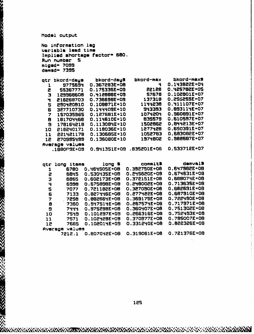
Model output
No information lagVariable lead timeImplied shortage factor- 580.Run number Smigud- 7099demsd- 7395
qtr bkord-daWs bkord-daWS bkord-max bkord-maxS1 9775694 0.367283E÷08 4 0.143822E+042 55367771 0.175335E609 a2128 0.'25782E+053 129968608 0.412888E+09 57678 0.102801E+07j 216268703 0.736658E+05 137318 0.2S52556E07S 290420810 0.108871E÷10 1144238 0.411107E6076 327710730 0.144409E÷10 943393 0.893114E6077 157035965 0.127581E+10 1074204 0.360891÷E078 181704468 0.114610E+10 835579 0.610597E÷079 178164218 0.113084E+10 1502862 0.844213E+07
10 218240171 0.118036E+10 1277428 0.650391E+0711 221421178 0.130585E+10 1052783 0.683082E+0712 270995•99 0.136080E+10 1974802 0.988687E+07
Average values.1880P9E÷09 0.941351E+09 .835201E606 0.533712E+07
qtr long items long 5 commits demvalS1 6780 0.465505E+08 0.392750E÷08 0.647982E+082 S845 0.530435E+08 0.2e5620E÷08 0.674631E+083 6865 0.602173E+08 0.372151E+08 0.688074E+08S6998 0.675898E608 0.248002E÷08 0.713635E+08S 7077 0.721182E+08 0.327090E÷08 0.682691E+086 7133 0.82746E4+08 0.277422E+08 0.687910E+087 7258 0.882664E÷08 0.369179E+08 0.722L90E+088 7350 0.9S7S1LE+08 0.26757'E÷08 0.717971E+089 7444 0.975298E+08 0.360407E+08 0.751302E+08
10 75'9 0.101297E+03 0.266316E+08 0.752493E+0811 7571 0.102286E+09 0.370977E+08 0.795007E÷0812 7665 0.102014E+09 0.331240E+08 0.822326E+08
Average values7212.1 0.807042E+O8 0.319061E+08 0.721376E+08
125
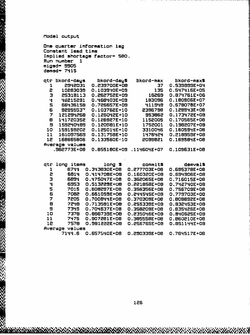
Model output
One quarter information logConstant lead timeImplied shortage factor- 580.Run number 1migsd- 9905demsd- 7415
qtr bkord-days bkord-dayS bkord-max bkord-maxS1 2542031 0.239700E+08 37 0.539899E+042 10283039 0.1039'tOE+09 135 0.547416E+053 25318113 0.2627S2E÷09 16269 0.874761E+061 46215291 0.i68'03E+09 183096 0.180906E+07S 66436158 0.726657E+09 411i4B 0.678078E+076 92955539 0.103762E+10 2396798 0.128953E+087 121295268 0.126042E+10 953862 0.173472E+088 141720352 0.126927E+10 1152005 0.170565E+089 1592O0i89 0.120581E+10 1752001 0.190207E+08
10 159159202 0.125014E+10 33100k6 0.16059OE+0B11 16109756 0.131758E+10 1476424 0.218955E+0812 168665B06 0.133560E-10 2095821 0.169584E+08
Average values.962773E+08 0.855180E+09 .114604E+07 0.109631E+08
qtr long items long S commits demvalS1 6744 0.343830E+08 0.277703E+OB 0.695378E+082 6814 0.41l708E+08 0.160320E+08 0.695906E+083 695Lt 0.LI750'7E+08 0.362065E+08 0.716015E+084 6953 0.513229E+08 0.221858E+08 0.74270E+085 7015 0.608297E+08 0.356356E÷08 0.756709E+086 70B2 0.661055E+08 0.245455E+08 0.779703E+007 7205 0.700804E+08 0.370305E+08 0.808892E+088 7248 0.713581E+08 0.255339E+08 0.832553E+089 734S 0.704637E+08 0.358205E+08 0.835426E+08
10 7378 0.B66739E+08 0.235046E÷08 0.840625E+0811 7475 0.907281E+08 0.385558E+08 0.860210E+0812 7578 0.981222E+08 0.256765E+08 0.651144E+08
Average values7144.6 0.657540E+08 0.290335E+08 0.784517E+08
126

--- -- ---- --1Model output
One quarter inf~ormation legConstant luad timeImplied shortage f~actor- 580.Run number 2migad- 5057demsd- 2873
qtr bkord-daUs bkord-daUS bkord-max bkord-maxS1 2'*930B9 0.293810E+08 73 0.199815E4-052 11722361 0.14k5336E+09 823 0.290168E+053 26'*B9305 0.3410756E+09 51675 0.BLI3GSLE+06Lj 53032177 0.S595&17E+09 250763 0.279996E+07S 90228637 0.820745SE+09 1061179 0.8'*282LiE+076 1417936060 0.112525E+10 1786068 0.156853E4-087 214*601037 0.1Li5200E+10 144LBSI*7 0.199790E+088 268181597 0.158029E+10 94j9831 0.14*5867E+089 32Li1SO45B 0.174*635E+10 14k650Li93 0.28B530E4-08
10 389101Lk57 0.187926E+10 2q*19111 0.32704i7E+0811 335905918 0.188212E4-10 3914*33L1 0.291929E+0812 25387ndbO 0.170352E+1.0 24*59205 0.2,10SB7E+08
Average v&lues.1764*77E+05 0.110844LE+2.0 .2411684iE+07 0.1LI8S18E+08
qtr long items long S commit$ damvalSU1 6772 0.3S2102E+00 0.304*942E+08 0.717272E+002 8827 0.'*1002!.E+0B 0.173S93E+08 0.730873E+083 6880 0.587932E+08 0.301373E+08 0.697890E+0O8It 6958B 0.03553'*E.08 0.210392E+-08 0.6944~10E+085 7039 0.7274I73E+08 0.3055E2E+OB 0.6878LI1E+06S 7135 0.775228E+OB 0.307328E+08 0.736257E+087 7220 0.83S'*36E+08 0.34I9892E+08 0.74I2770E+08B 7302 0.84I1368E+08 0.259366E+0B 0.777732E+089 74I02 0.931261E+08 0.360587E+08 0.754I772E+0810 7LI58 0.96674I6E+-08 0.270753E+0B 0.763Li4i4E+08
11 7510 0.933S52E+08 0.3264i15E1+08 0.783776E+0O812 7606 0.989276E+08 0.261899E+08 0.81B653F.+OB
kiverage values7175.8 0.7408561E+08 0.286130E+08 0.74i25L1E+08
127
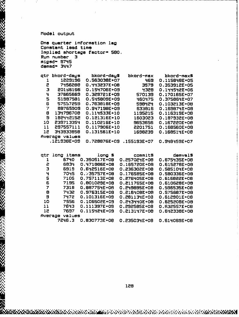
Model output
One quarter information lagConstant lead timeImplied shortage factor- 580.Run number 3migsd- 9745demsd- 34k7
qtr bkord-dass bkord-daUS bkord-max bkord-maxS1 1229196 0.563038E+07 469 0.11SB8E+052 7'56288 0.443237E+08 3579 0.353912E+053 20166166 0.15'706E+09 4328 0.144542E+06* 37665669 0.329721E+09 570139 0.170165E+075 51987561 0.545809E+09 460475 0.375866E+076 57557259 0.763818E+09 59802* 0.103213E+087 88765909 0.947198E+09 633816 0.169874E+088 134796708 0.114533E+10 1195215 0.116319E÷089 182442152 0.121316E+10 1603023 0.187932E+08
10 239713354 0.110216E+10 9653656 0.167220E+0811 297557111 0.117906E+10 2201751 0.168560E÷0812 343933858 0.131561E+10 1698239 0.168514E+08
Average values.121938E+09 0.728876E+09 .155193E+07 0.948iS9E+07
qtr long items long S commits demval$1 6740 0.350517E+08 0.257024E+08 0.675435E+082 6834 0.471886E+08 0.165720E+08 0.615278E+083 6919 0.6S2516E+08 0.236302E+08 0.585104E+08Li 7045 0.V35757E+08 0.176S85E+08 0.580336E+0B
5 7105 0.757113E+08 0.276405E+08 0.616822E+086 7195 0.801029E+08 0.211765E+08 0.610628E+087 7318 0.887754E+08 0.249895E+08 0.596535E+088 7432 0.976315E+08 0.216408E+08 0.575687E+089 7472 0.101316E+09 0.281134E+08 0.612901E+0810 7556 0.106502E+09 0.243440E+08 0.625208E+0811 7643 0.111397E+09 0.292585E+06 0.632557E+0812 7697 0.115424E+09 0.213147E+0B 0.642338E+08
Average values7246.3 0.830773E+08 0.235034E+08 0.614069E+08
128

Model output
One quarter information lagConstant lead timeImplied shortage factor- 560.Run number f
migsd- 1075demsd- 1175
qtr bkord-daUs bkord-daUS bkord-max bkord-maxS1 3468927 o.49S55E+OB 652 0.199509E+052 14275248 0.138239E+09 714 0.233083E+063 33269461 0.445949E+09 52895 0.156054E+074 54905350 0.770390E+09 678605 0.374979E+07S 7716859k 0.104341E+10 951505 0.173288E+086 92753127 0.132842E+10 957623 0.187711E+087 118091935 0.162170E+10 894362 0.209070E+088 1465959B4 0.162567E+10 1SO94SS 0.245741E+089 155287640 0.167391E÷10 1987206 0.225735E+08
10 179644817 0.159998E÷10 e08530 0.176064E+0811 204757323 0.177544E÷10 4480711 0.262410E+0812 207169339 0.161732E÷10 1669692 0.281149E+08
Average values.107281E+09 0.114586E+10 .127233E+07 0.151400E+08
qtr long items long S commits demvalS1 6772 0.350411E+08 0.29782'IE+08 0.72671BE+082 681 0.400672E+08 0.173SS7E+O8 0.751768E+083 6962 0.k57825E+08 0.36628E÷B08 0.774171E+084 7061 0.523625E+08 0.209844E+08 0.770944E+085 7100 0.581866E+08 0.346724E+08 0.742661E+086 7203 0.653577E+0B 0.256740E+08 0.742950E+087 7251 0.680109E+08 0.365270E+08 0.770744E+088 7366 0.745585E+08 0.259241E+08 0.808415E÷089 7407 0.825981E+08 0.375058E+08 0.791643E+08
10 7485 0.801343E÷08 0.273855E+08 0.802358E+0811 7552 0.918083E+08 0.360398E+08 0.792118E+0812 7626 0.102589E+09 0.267409F+08 0.765405E+08
Average values7218.8 0.662914E+08 0.295931E+08 0.769991E+08
129
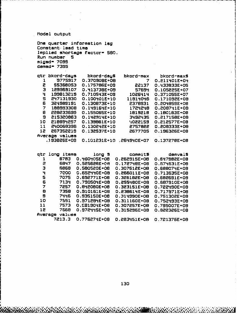
Model output
One quarter information lagConstant lead timeImplied shortage factor- 580.Run number 5migsd- 7095demsd- 7395
qtr bkord-dags bkord-daU$ bkord-max bkord-maxS1 9775917 0.370908E+08 7 0.211401E+042 55368053 0.175786E+09 22137 0.433833E+053 129969107 0.413738E+09 57659 0.10522SE÷074 199813219 0.7105'3E+09 1026514 0.371055E+07S 247131930 0.100401E+10 11814046 0.171092E+0B6 324989191 0.130873E÷10 2378531 0.204859E+087 188993308 0.148164E+10 172424B 0.208741E+088 228233699 0.155065E+10 1819218 0.180163E+069 215320863 0.142914E+10 3492435 0.21715BE÷08
10 21BB54257 0.139861E+10 'i022159 0.212577E+0811 240068396 0.1302q2E+10 2757822 0.208333E÷0812 267352219 0.132537E+10 2677705 0.196326E+08
Average values.193826E+09 0.101231E+10 .264940E+07 0.137278E+08
qtr long items long $ commits demvail$1 6783 0.'6040SE÷08 O.2B291SE+08 0.647982E+082 6847 0.52S628E+0C 0.172748E+0 0.674631E+083 6868 0.580520E+08 0.307612E+08 0.688074E+08Lt 7000 0.6524i0E+08 0.266011E+08 0.713635E+085 7075 0.652771E+08 0.326182E+08 0.682691E+086 7134 0.79050'E+08 0.255L80E+08 0.687910E+087 7257 0.842080E÷08 0.323151E+08 0.722590E+088 7358 0.910161E+08 0.238614E+08 0.717571E+089 7446 0.935150E+08 0.314950E+08 0.751302E+08
10 7551 0.971284E+08 0.311160E+08 0.752593E÷0811 7573 0.5981904E+08 0.307257E+08 0.795007E+0812 7668 0.972S'5E÷08 0.315296E+08 0.822326E"-0B
Average values7213.3 0.776274E+08 0.283451E+08 0.721376E+08
130
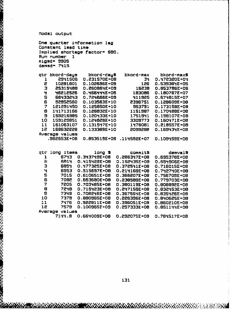
Model output
One quarter information lagConstant lead timeImplied shortage factor- 560.Run number 1migsd- 9905demsd- 7*15
qtr bkord-days bkord-daUS bkord-max bkord-maxS1 2941S06 O.231S70E+08 34 0.472320E+042 10281801 0.102696E+09 126 O.S3936SE+053 2531s58e 0.2S0864E+09 16238 0.853786E+064 46212S26 0.466S54E÷09 183086 0.180767E+07S 66S33243 0.72*565E+09 41192S 0.67481SE+076 92952550 0.103S63E+10 23967S1 0.128609E+087 121291450 0.125860E+10 953791 0.173168E+088 141713166 0.12S632E410 1151987 0.170488E÷089 159216985 0.120433E+10 1751941 0.198107E+08
10 159129851 0.124828E+10 3309773 0.160471E+0811 161053107 0.131657E+10 1476081 0.21B557E+0B12 168632228 0.133389E+10 2099288 0.169434E÷08
Average values.962653E+08 0.853519E÷09 .11'592E+07 0.109'59E+O8
qtr long items long S commits demvalS1 6743 0.343749E+08 0.286347E+08 0.695378+E082 6814 0.415*22E+08 0.152435E+08 0.694906E+083 589L 0.477325E+08 0.372651E+08 0.716015£E084 6953 0.515697E+08 0.214169E+08 0.74270E+08S 7015 0.610651E+08 0.366207E+08 C.756709E+086 7082 0.663680E+08 0.23858£E÷08 0.779703E+087 7205 0.703'BSE+08 0.380119E+08 0.808892E+08a 7248 0.716423E÷OB 0.2'7169E+08 0.832'53E+OB9 7349 0.708246E+08 0.367655E08 0.836526E+08
10 7379 0.88096SE+08 0.226396E+08 0.840625E+OB11 7476 0.922811E+08 0.396051E+08 0.860210E+0812 7S79 0.100966E+09 0.257333E+08 0.861144E+08
Average values7144.8 0.66'009E+08 0.292075E+08 0.78L517E+08
131
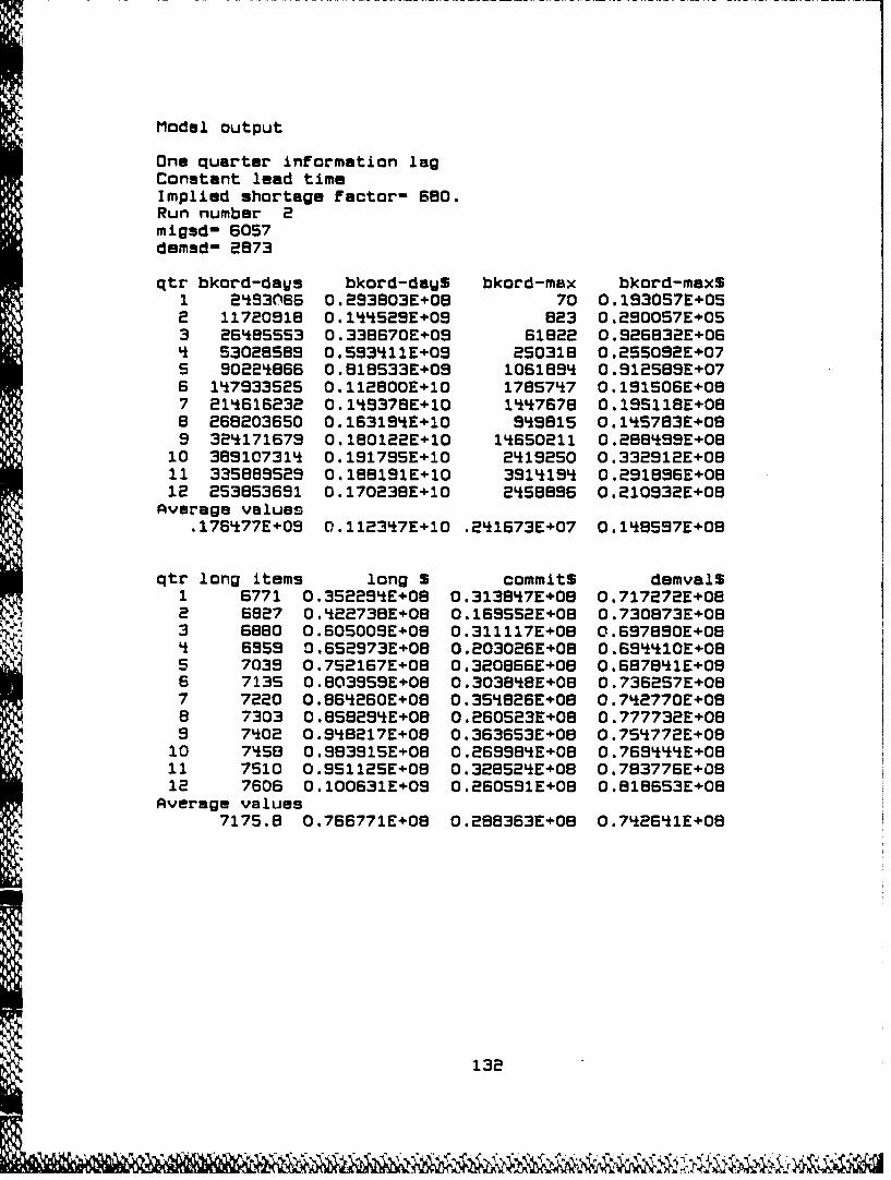
Model output
One quarter information lagConstant lead timeImplied shortage factor- 6BO.Run number 2migsd- 6057demsd- 2B73
qtr bkord-da~s bkord-daUS bkord-max bkord-maxS1 2'93066 0.293803E+08 70 0.193057E+052 11720918 0.144529E+09 823 0.290057E+053 26585553 0.33B670E+09 61822 0.926B32E+064 53028589 0.593411E+09 250318 0.255092E+075 90224866 0.81B533E+09 1061899 0.912589E+076 147933525 0.112800E+10 1785747 0.191506E+087 214616232 0.149378E+10 1447678 0.19S118E+088 268203650 0.163194E+10 959815 0.145783E+089 324171679 0.180122E+10 1k650211 0.288499E+08
10 389107314 0.191795E+10 2419250 0.332912E+0811 335889529 0.188191E+10 3914194 0.291896E+0812 253853691 0.170238E+10 2L58896 0.210932E+08
Average values.176477E+09 0.112347E+10 .241673E+07 0.1L9597E+08
qtr long items long S commits demvalS1 6771 0.35229E+÷08 0.313847E+08 0.717272E+082 6827 0.422738E+08 0.1695S2E+08 0.730873E+083 6880 0.505009E+08 0.311117E+08 0.6978900E+B4 6959 0.652973E+08 0.203026E+08 0.694410E+085 7039 0.752167E+08 0.320866E+08 0.687841E+086 7135 0.803959E+08 0.303848E+08 0.7362S7E+087 7220 0.864260E+08 0.35L826E+08 0.742770E+088 7303 0.85829LE+08 0.260523E+08 0.777732E÷089 7402 0.948217E+08 0.363653E+08 0.754772E+08
10 7L56 0.993915E+08 0.269984E+08 0.769444E+0811 7510 0.951125E+08 0.328524E+08 0.783776E+0812 7606 0.100631E+09 0.260S91E+08 0.81B8S3E+OB
Average values7175.8 0.766771E+08 0.288363E+08 0.742641E+08
132

Model output
One quarter information lagConstant lead timeImplied shortage factor- 680.Run number 3migsd- 9745demsd- 3447
qtr bkord-days bkord-daWS bkord-max bkord-max$1 1229193 0.562970E+07 466 0.10SOSOE+052 7456279 0.443229E+08 3570 0.345898E+053 20156106 0.154647E+09 *325 0.143B37E+064 3766578 0.325452E+09 570139 0.170163E+07S 51886605 0.$5L246E+09 460469 0.375345E+076 57555981 0.761876E+09 598411 0.102986E+087 88764021 0.9L4675E÷0S 633810 0.169B33E+088 134795151 0.114351E+10 1185159 0.116063E+089 1B2437757 0.121075E+10 1602952 0.187660E+08
10 239701444 0.110108E+10 9653502 0.166652E+0811 2975429L3 0.117775E+10 2201696 0.16B159E+0812 343S20056 0.131493E+10 1698113 0.168478E+08
Average values.121934E÷09 0.727740E+09 .15518SE+07 0.946896E+07
qtr long items long S commits demvalS1 6739 0.350501E+08 0.265735E+08 3.675435E+082 6834 0.47563E+08 0.157843E+08 0.615278E+083 6919 0.6i9916E+08 0.236475E+08 0.$85104E+08L 705S 0.743056E÷08 0.178385E+08 0.580336E+08S 7105 0.764458E+08 0.277654E+08 0.616822E+086 7195 0.BOB12E+08 0.211764E+08 0.610628E+087 7317 -. 895619E+08 0.250318E+08 0.596535E+08a 7431 •.986723E÷03 0.217814E+08 0.$75687E+089 7472 0.102437E+09 0.28178SE+08 0.612901E+0810 7SSS 0.107672E+09 0.245100E+08 0.625208E+0811 7643 0.112574E+09 0.293677E+08 0.632557E+0812 7697 0.116701E+09 0.214293E+08 0.642338E+OB
Average values72i6.1 0.839017E+08 0.235903E+08 0.614069E+08
133
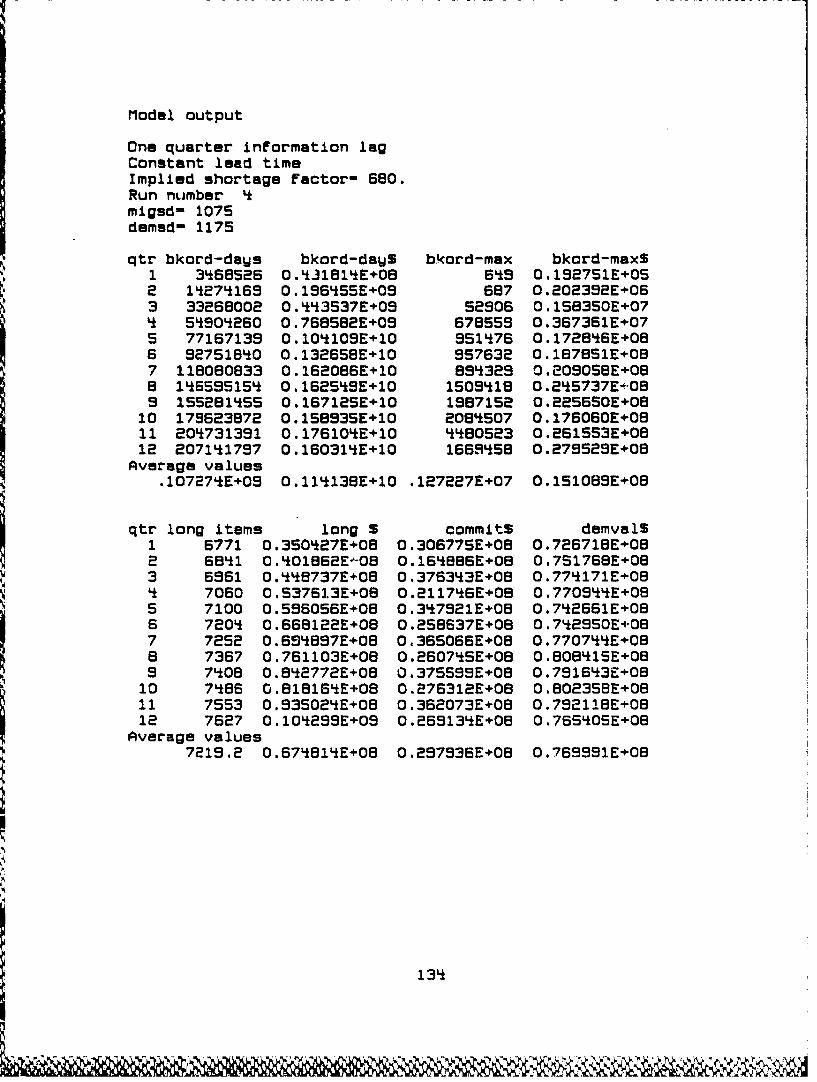
Modal output
One quarter information lagConstant lead timeImplied shortage factor- 680.Run number k
migsd- 1075demad- 1175
qtr bkord-daus bkord-daWS bkord-max bkord-maxS1 3466526 0.431B1LE+08 649 0.192751E+052 14271659 0.196555E+09 687 0.202352E÷063 33268002 0.443537E+09 52906 0.15B350E÷07Lj 54904260 0.768582E+09 676555 0.367361E+075 77167139 0.104109E+10 951476 0.172846E÷086 92751850 0.132558E+10 957632 0.187851E+087 118080833 0.162086E÷10 89329 0.20905BE+088 1*6595151 0.162519E+10 1509418 0.245737E°08S l55281555 0.167125E+10 1987152 0.225650E+08
10 179623872 0.158935E+10 2084507 0.176060E+0811 204731391 0.176104E+10 44B0523 0.261553E+0812 207141797 0.160314E+10 1665956 0.279529E+08
Average values.107271E+09 0.114138E+10 .127227E÷07 0.151OBSE+08
qtr long items long S commits demvalS1 6771 0.350127E+08 0.306775E+08 0.726718E+08S681 0.401862E-08 0.1648B6E+08 0.75176BE+083 6561 0.448737E+08 0.376343E+08 0.774171E÷08
ki 7060 0.$3761.3E+08 0.211746E÷08 0.770944E÷08S 7100 0.S95056E+08 0.347921E*08 0.742661E÷08
6 7204 0.668122E+08 0.258637E+08 0.792150E+087 7252 0.694897E+08 0.365066E+08 0.770744E+08a 7367 0.761103E+08 O.2SO745E÷08 0.80841E+08S 7408 0.842772E+08 0.3755SSE÷08 0.791643E÷08
S10 7486 0.818164E+08 0.276312E+08 O.8oe35BE÷OBS11 7553 0.935024E+08 0.362073E+08 0.7S21!8E+08
12 7627 0.104299E+09 0.26S134E÷08 0.765S05E+08Average values
721S.2 0.674814E+08 0.297S36E÷08 0.769391E+08
134
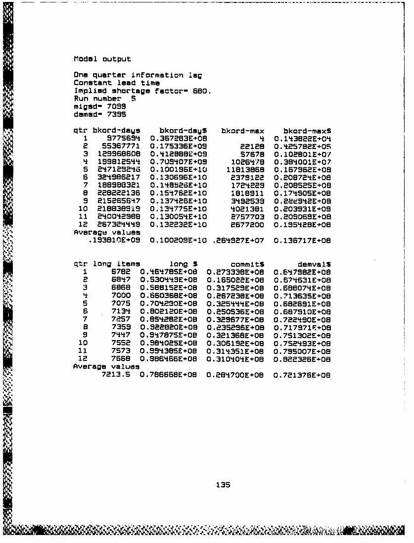
Model output
One quarter information lagConstant lead timeImplied shortage factor- 680.Run number Smigsd- 7099demsd- 7395
qtr bkord-days bkord-daUS bkord-max bkord-maxS1 9775694 0.367283E+08 k 0.143822E+042 S5367771 0.17S336E÷09 22128 0.425782E+053 129968608 0.412888E+09 57678 0.102801E+074 139812544 0.709'07E+09 1026S78 0.385001E+075 247129248 0.100196E+10 11813868 0.167962E+086 32'986217 0.130696E+10 2379122 0.208724E+087 18898B321 0.148926E+10 1724229 0.208525E+088 228222136 0.154762E+10 1818911 0.17490S5E089 2152656S7 0.137426E+10 3492539 0.22d942E+08
10 218838919 0.13577SE÷10 *021381 0.203931E+0911 240042988 0.1300S'E+10 2757703 0.209069E+0812 267324449 0.132232E+10 2677200 0.195428E+08
Average values.193810E+09 0.100209E+10 .264927E+07 0.136717E+08
qtr long items long S commits demvalS1 6782 0.464785E+08 0.273338E+08 0.647982E+082 6847 0.530449E+08 0.165022E+08 0.674631E+083 6868 0.588152E+08 0.317529E+08 0.688074E+084 7000 0.660368E+08 0.267238E+08 0.713635E+085 7075 0.704290E+08 0.32544E+÷08 0.682691E÷086 7134 0.802120E+08 0.250536E+08 0.687910E÷087 72S7 0.854282E+08 0.329677E+08 0.722490E+08a 7359 0.922820E+08 0.235296E+08 0.717971E+089 7447 0.94787sE+08 0.321368E+08 0.751302E+08
10 7552 0.984025E+08 0.306192E+08 0.7S2493E+0811 7573 0.994385E+08 0.314351E+08 0.795007E+0812 7668 0.986466E+08 0.310404E+0B 0.822326E+08
Average values7213.S 0.786668E+08 0.284700E+08 0.721376E+08
135
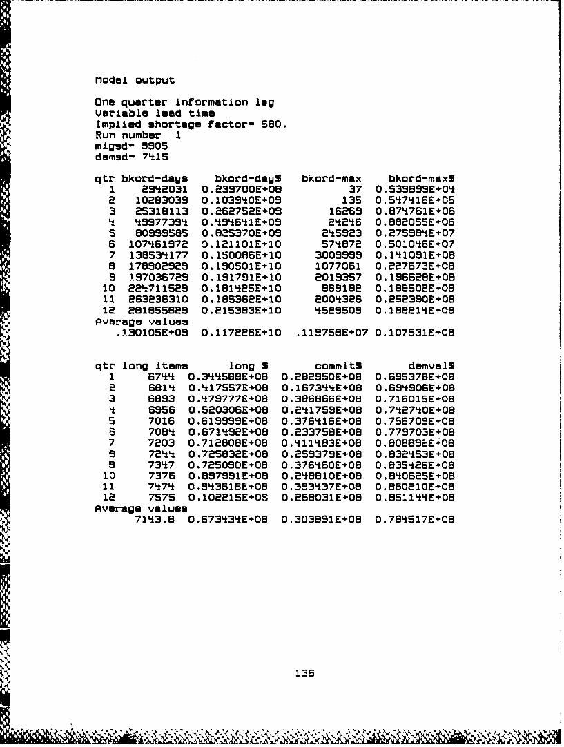
Model output
One quarter information legUariable lead timeImplied shortage factor- 580.Run number 1migsd- 9905demsd- 7415
qtr bkord-daWs bkord-daWS bKord-max bkord-maxS1 2942031 0.239700E÷08 37 0.539899E÷042 10283039 0.103950E+09 135 0.547416E÷053 25318113 0.262752E+09 16269 0.874761E+06* 45977394 0.*94641E+09 24256 0.882055E÷06S 80995865 O.82S370E+09 2'5923 0.27598*E÷076 107451972 0.121101E÷10 574872 0.S010L6E+077 138534177 0.150086E+10 3009999 0.141091E+08B 178902929 0.190501E*10 1077061 0.227673E÷08S1,97036729 0.191791E÷10 2019357 0.195628E+08
10 224711529 0.101425E+10 869182 0.188502E÷0811 263236310 0.18S362E+10 2004326 0.252390E÷0812 281855629 O.215383E+10 4529509 0.188214E+08
Average values.1,30105E+09 0.117226E+10 .119758E+07 0.107531E+08
qtr long items long S commits demvalS1 6744 0.344556E+06 0.282950E+08 0.695378E+08a 6814 0.417557E+08 0.167344E÷08 0.694906E+083 6893 0.479777E+08 0.386B66E+08 0.716015E÷08'k 6956 0.520306E+08 0.241759E+08 0.742740E+085 7016 0.619999E÷08 0.376S16E+08 0.756709E+OB6 7084 0.671492E+08 0.233758E÷08 0.779703E+087 7203 0.712808E+08 0.411483E+06 0.80BB9EE+088 7244 0.72S532E+08 0.259379E+08 0.832453E+089 7347 0.725090E+08 0.376560E÷08 0.835426E+08
10 7376 0,897991E+08 0.248810E+08 0.840625E+OB11 747* 0.943616E÷08 0.393337E+OB 0.860210E+0812 7575 0.102215E+00 0.268031E+08 0.BS1144E+08
Average values7143.8 0.67343'E+OB 0.303891E+08 0.784517E+08
136
~Aft
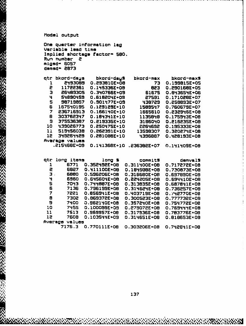
Model output
One quarter information lagVariable lead timeImplimd shortage factor- 580.Run number 2migsd- 6057demsd- 2873
qtr bkord-dajs bkord-daWS bkord-max bkord-maxS1 2493089 0.253810E+08 73 0.199815E÷052 11722361 0.145336E+05 823 0.290168E6053 26489305 0.340766E÷09 61675 0.84365LE+064 54890L59 0.618204E÷09 27551 0.171028E+075 9871S957 0.901177E+09 436725 O.258893E÷076 167540195 0.129129E+1O 1585'7 0.760679E+077 236716913 0.1661I40E10 1665610 0.232946E+08B 303762347 0.184341E÷10 113558L 0.1759'3E÷089 375536387 0.219335E+10 3186040 0.21623SE÷0O
10 439026773 0.250L75E+10 22S6692 0.195333E÷0811 515L56038 0.262391E+10 13598307 0.320274E+0812 349264429 0.281088E÷10 3956887 0.428193E+08
Average values.• 15L68E+09 0.1L1368E+10 .236382E+07 0.141409E+08
qtr long items long S commits demvalS1 6771 0.352L92E+08 0.311400E+08 0.717272E÷08a 6827 0.411100E÷08 0.18LSBEe08 0.730873E+083. 6880 0.596205E+08 0.316680E+08 0.697830E+08L 6960 0.6i5560L+08 0.224205E+08 0.695L10E+085 7043 0.7448876+08 0.313835E÷08 0.5878L1E+086 7136 0.796199E+08 0.31'524E+08 0.7362S7E4087 7221 0.856941E+08 0.403719E+08 0./L2770E+08B 7302 0.B65372E+08 0.300523E+08 0.777732E+089 7400 0.S621L0E+08 0.357240E+08 0.75i772E+08
10 7455 0.100099E'09 0.273072E+OB 0.769444E+0811 7513 0.969957E÷08 0.317936SE08 0.783776E+0B12 7608 0.1035S4Es09 0.31i651+08 0.B18653E408
Average values7176.3 0.770111E+08 0.303206E+08 0.7426i1E+08
137
S.N

Model output
One quarter informatlon lagVariable lead timeImplied shortage factor- SO0.Run number 3migsd 975Sdemsd- 3*47
qtr bkord-daus bkord-daWS bkord-max bkord-maxS1 1229196 0.563038E+07 569 0.115SB8E+052 756288 0.443237E÷08 3579 0.353912E+053 20156166 0.154706E+09 *328 0.145'52E+064 38651104 0.336631E+09 *356 0.351976E+06
5 56559025 O.5752'1E09 819093 0.330167E+076 74392695 O.B59265÷E09 819643 0.61093SE+077 99590088 O.111562E+10 628347 0.101216E+088 154535*98 0.132692E+10 553560 0.119291E+089 214916768 0.155714E+10 1*31563 0.223205E+08
10 284*05912 0.165175E+10 1313336 0.135120E+0811 34e697757 0.172607E+10 182S675 0.182275E60812 410168559 0.186035E+10 5817486 0.202243E+05
Average values.14253SE+09 0.933625E÷09 .107321E+07 0.865746E+07
qtr long items long S commits demvalS1 S74*0 0.350957E+08 0,258003E+08 0.S75'*3SE+062 6832 0.473382E+08 0.172911E+08 0.61S278E+083 6918 0.6451197+08 0.,!44643E+08 0.58510Lý2+08
7042 0.739S63A+08 0.i795'7E+08 0.580336E+085 7104 0.765256E+06 0.287625E+08 0.616822E+086 7196 0.812106E+08 0.236910E+0B O.510628E+087 7318 0.906077E+08 0.260040E+08 0.596535E+088 7430 0.100914E+09 0.227773E÷08 0.575687E+089 7471 0.105087E+09 0.256878E+08 0.612901E+08
10 7555 0.110947E209 0.271735E+08 0.625208E+0811 7643 0.115921E+09 0.294017E+08 O.632557E+0812 7696 0.121014E+09 0.2844'8E+OB 0.642338E+08
Average values7245.4 0.852359E+08 0.247877E+08 0.614069E+08
IS~138
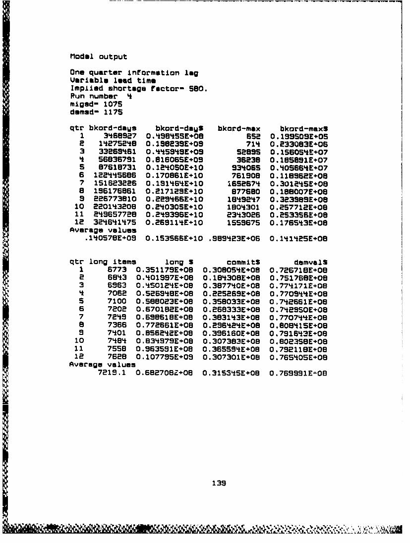
Model output
One quarter information lagUariabli 1usd timeImplied shortage factor- 580.Run number 4migad- 1075domed- 1175
qtr bkord-daWs bkord-dayS bkord-mmx bkord-maxS1 3468927 O.458*55÷E08 652 0.199509E+052 1t2752'8 0.1S823SE+O9 714 0.e33083E+O63 3326S461 0.45594SEOS 52895 0.156SOSE+074 56836791 0.81606SE÷05 36238 0.185651E+07S 87618731 0.124050E+10 S34065 0.*0566S*E076 122'456S6 0.170861E+10 761908 0.115562E+087 151623226 0.191464E÷10 I655674 0.30124SE088 156176861 0.217129E+10 877680 0.188007E+089 226773810 0.224966E+10 1849247 0.323989E08
10 220143208 0.240305E+10 1804301 0.257712E+0811 24S657728 0.249396E+10 2343026 0.253356÷E0812 324641475 0.269114E+10 1555675 0.176543E+08
Average values.140578E+09 0.153566E+10 .989423E+06 0.14125E+08
qtr long items long S commits demvalS1 6773 0.35117SE£08 0.308054tE08 0.726718E+082 6843 0.401997E+08 0.1843086E08 0.751768÷E4083 6963 0.450124E+08 0.387740E+08 0.77k171E+06S7062 0.5265LBE+08 0.225269E+08 0.7709S4tE+0BS 7100 0.5B8023E+OB 0.359033E+08 0.742661E+086 7202 0.670182E+08 0.268333E+08 0.702SSOE+087 72S 0.69861BE+08 0.383143E+08 0.77074*&E÷05a 7366 0.772661E+09 0.296424E+08 0.808415E+089 7401 0.856242E+08 0.396160E+08 0.791643E+08
10 74B4 0.93"979E608 0.307383E+08 0.802358E+0811 7558 0.963591E+08 0.36559tE+09 0.7521186E+012 7628 0.107795E+09 0.307301E608 0.7650SE+08
Average values7219.1 0.68270eZ+08 0.315345E+08 0.769S91E08
135

Model output
One quarter information lagUariable lead timeImplied shortage factor- 580.Run number Smig3d- 7099demsd- 7395
qtr bkord-dams bkord-day$ bkord-max bkord-max$1 9775917 0.370908E+08 7 0.211401E+042 55368053 0.175786E+09 22137 0.433833E+053 129969107 0.413738E+09 S7694 0.105225E+07k 216259350 0.737800E+09 137254 0.242308E+07S 295233538 0.110690E+10 1585139 0.374998E+076 353590205 0.153665E*10 2094665 0.872056E+077 216873BS6 0.174183E+10 2479423 0.257933E+088 272233848 0.20095'E+10 2184133 o.263354E+089 307956575 0.215904E+10 3243001 O.220052E+08
10 314397706 0.208445E+10 2392517 0.260202E+0811 332023650 0.2041BSE+10 4325631 0.198226E+0812 059102947 0.223014E+10 3764192 0.255708E+08
Average values.242740E+09 0.135623E+10 .185715E+07 0.134616E+08
qtr long items long S commits demvalS1 5784 0.460798E+08 0.268584E+08 0.647982E+082 6848 0.526533E+0B 0.18254!E+08 0.674631E+083 6868 0.584696E+08 0.327610E+08 0.688074E+08f 6998 0.658106E+08 0.280799E+08 0.713635E+085 7076 0.700979E+08 0.345732E+08 0.6B2691E+086 7131 0.802370E+08 0.2e1953E+08 0.687910E+087 7256 0.862283E+08 0.361052E+08 0.722490E+088 7357 0.937105E+08 0.271517E+OB 0.717971E+089 7446 0.965119E+08 0.338535E+08 0.751302E+08
10 7551 0.100147E+09 0.32&282E+OB 0.752493E+0811 7574 0.101470E+09 0.306549E+08 O.795007E+0B12 7668 0.101496E÷09 0.363S84E+08 0.822326E+08
Average values7213.1 0.79094E+08 0.301228E+08 0.721376E÷08
iLt0

Model output
One quarter information lagVariable lead timeImplied shortage factor- 680.Run number 1migsd- 9905demsd- 7415
qtr bkord-daes bkord-daWS bkord-max bkord-max$1 2S'1506 0.231S70E+08 34 0.472320E+042 1OR81801 0.102696E+09 126 0.$39365E+053 26315'8B 0.260864E+09 16238 O.853786E+06L 49974685 0.492683E+09 24236 0.880672E+06S 80996688 0.823378E+09 2*5919 0.275807E+076 1074590S1 0.120902E+10 577835 0.498331E÷077 138531047 0.149878E+10 3009967 0.140651E+068 178893295 0.1902S3E+10 1076991 0.227413E+089 197013760 0.191653E+10 2019329 0.196"453E+08
10 224683312 0.181240E+10 868905 0.188402E+0811 263197874 O.185168E+10 2004274 0.2S2376E+0812 281813328 0.215107E+10 5532352 0.188191E+08
Average values.130092E÷09 0.117040E+10 .119782E+07 0.107408E+08
qtr long items long S commits demval$1 6743 0.34*507E+08 0.291611E+08 0.695378E+082 6814 0.418335E÷08 0.19SS12E+08 0.694906E+083 6893 0.482171E+08 0.397879E+08 0.716015E+084 6956 0.522850E+08 0.234225E+08 0.7",2740E+085 7016 0.622508E+08 0.386655E+08 0.756709E+086 7084 0.674213E+08 0.227760E+08 0.779703E+067 7203 0.715534E+08 0.421827E+08 0.808892E+088 7243 0.728841E+08 0.261430E+08 0.832453E+089 7347 0.729121E+08 0.385992E+08 0.835426E+08
10 7377 0.912807E+08 0.240321E+08 0.840625E+0811 7475 O.959820E+08 0.404104E+08 0.860210E+0812 7S76 0.105143E+09 0.269201E+08 0.8511'*E+08
Average values7143.9 0.680186E+08 0.305876E+08 0.784517E+08
1L*1
•••- - •"" • , - •- ,?•• .. -,. •• •••"•,
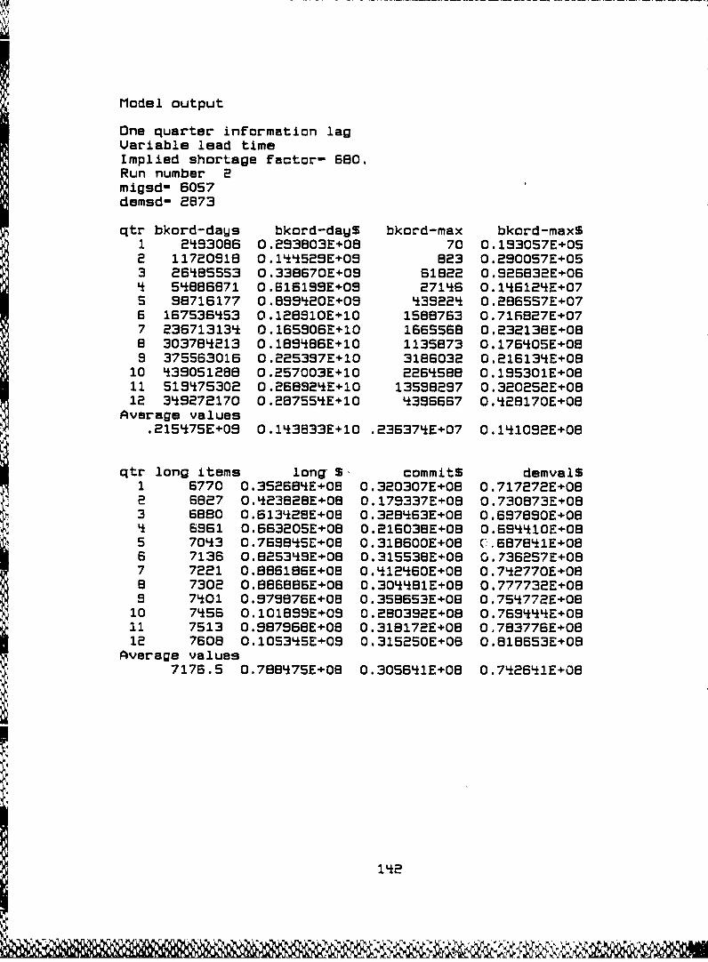
Model output
One quarter information lagUariable lead timeImplied shortage factor- 680.Run number 2migsd- 6057demsd- 2873
qtr bkord-days bkord-dawS bkord-max bkord-maxS1 2493086 0.293803E+08 70 0.193057E+052 11720918 0.144529E+09 823 0.290057E+053 26'85553 0.338670E+09 61822 0.926832E+06L 54886871 0.616199E+09 27146 0.1k6124E+07S 98716177 08.99420E+09 438224 0.286557E+076 167536S53 0.128910E+10 1588763 0.716827E÷077 23671313Li 0.165906E+10 1665568 0.232138E+088 303784213 0.189486E+10 1135873 0.176405E+089 375563016 0.225397E+10 3186032 0.21613'E+08
10 *39051288 0.257003E+10 226558B 0.195301E+0811 519475302 0.268924E+10 13598297 0.320252E÷0812 349272170 0.28755*E+10 4396667 0.428170E+08
Average values.215475E+09 0.143833E+10 .236374E+07 0.1410O2E+08
qtr long items long S- commits demval$1 6770 0.352684E+08 0.320307E+08 0.717272E+082 6827 0.423828E*08 0.179337E+0B 0.730873E+083 6880 0.613128E+08 0.328463E+08 0.697890E+08S6961 0.663205E+08 0.216038E+0B 0.694410E+085 7043 0.769885E+0B 0.318600E+08 C 687841E+086 7136 0.825348E+08 0.315S38E+08 0.7362S7E+087 7221 0.886186E+08 0.412460E+08 0.742770E+08a 7302 0.886886E+08 0.304481E+08 0.777732E÷088 7401 0.979876E+08 0.358653E+02 0.7Sk772E+08
10 7456 0.101BSSE+09 0.280392E+08 0.769444E+0811 7513 0.987968E+08 0.318172E+08 0,783776E+0812 7608 0.105345E+08 0.315250E+0B 0.818653E+08
Average values7176.5 0.788475E+08 0.305641E+08 0.742641E+08
142
1116101 1 162
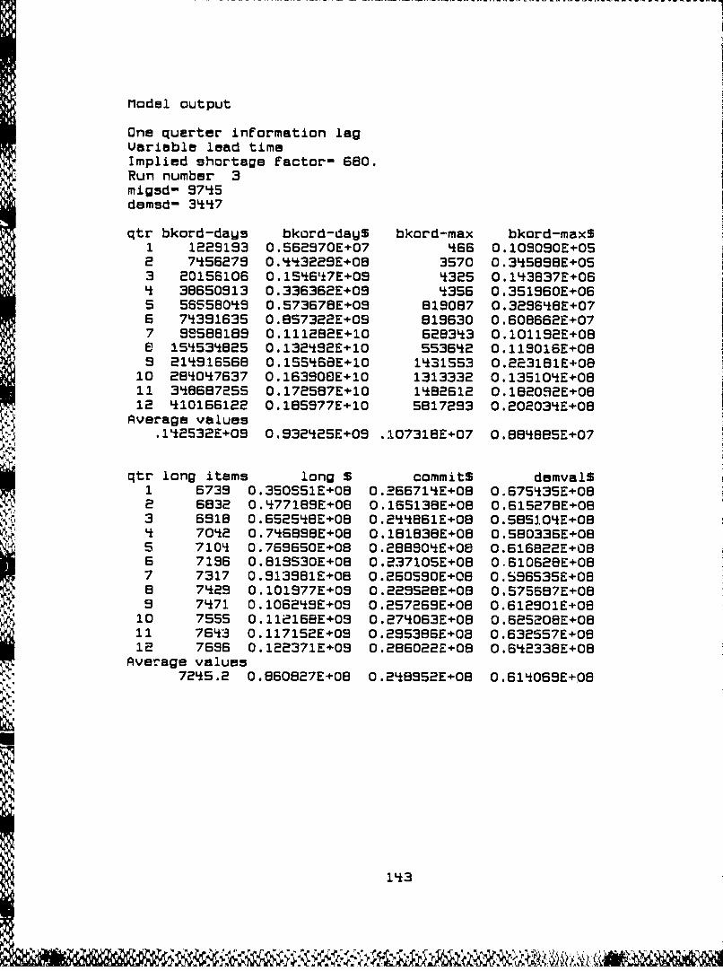
Model output
One quarter information lagVariable lead timeImplied shortage factor- 680.Run number 3migsd- 5745demsd- 3447
qtr bkord-daus bkord-dayS bkord-max bkord-maxS1 1229193 0.562970E+07 466 0.103090E+052 7456279 0.443229E+08 3570 0.345898E+053 20156106 0.15'*6,t7E+09 4325 0.1'3837E+064 38650913 0.336362E+09 '356 0.351960E+06S 56558048 0.573678E+09 819087 0.32968E+076 74391635 0.857322E+0S 819630 0.608662E+077 S588189 0.111282E+10 628343 0.101192E+08E 154534825 0.132492E+10 553642 0.119016E+089 214916568 0.155468E÷10 1431553 0.223181E+08
10 284047637 0.163908E+10 1313332 0.135104E+0811 3'8687255 0. 172587E+10 1482612 0.182092E+0812 410166122 0.185977E÷10 5817293 0.202034E+08
Average values.112532E+09 0.932425E+09 .107318E+07 0.886885E+07
qtr long items long $ commits demval$1 6739 0.350S51E+0B 0.266714E+08 0.675435E+082 6832 0.477189E+08 0.165138E+08 0.615278E+083 6918 0.652548E+08 0.244861E+08 0.585104E+084 7042 0.756888E+08 0.181838E+08 0.580336E+085 7104 0.769650E+08 0.288904E+08 0.616822E+086 7196 0.819530E+08 0.237105E+08 0.610628E+087 7317 0.913981E+08 0.260590E+08 0.56535E+08a 7429 0.101977E+09 0.229S28E+08 0.575687E+089 7471 0.106248E+03 0.257269E+08 0.612901E+08
10 7555 0.112168E+09 0.274063E+08 0.625208E+0811 7643 0.117152E+09 0.295386E+03 0.632557E+0812 7696 0.122371E+09 0.286022E+08 0.642338E+08
Average values7245.2 0.860827E+08 0.248952E+08 0.614069E+08
143
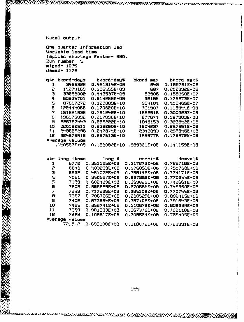
I'iodel output
One quarter information lagVariable lead timeImplied shortage factor- 680.Run number 4migsd- 1075demsd- 1175
qtr bkord-daUs bkord-daW$ bkord-max bkord-maxS1 3*68525 0.491814E÷08 649 0.1E27S1E+OS2 14274169 0.1964SSE+09 687 0.?02392E+063 33286002 0.443537E+09 52906 0.158350E+074 56835701 O.8142SeE÷09 36192 0.178273E+075 87617272 0.123809E+1O 934104 0.412465E+076 1224k4066 0.170620E+10 7C1907 0.118944E+087 IS162163S 0.191242E+10 1652616 0.300323E+088 196176092 0.217096E+10 877674 0.187903E,089 226767443 O.229222E+10 18491S3 0,323842E+08
10 220122511 0.239260E+10 1804257 0.257651E+0811 249629298 0.247874E*10 2348B93 0.252846E+0812 324575516 0.267513E+10 1558776 0.175272E+08
Average values.1*0567E÷09 0.153082E+10 .965321E+06 0.141159E+08
qtr long items long S commits demvalS1 6772 0.351195E+08 0.317275E+08 0.726718E+082 6843 0.403238E÷08 0.1760S3E+0b 0.751768E+083 6Se2 0.451072E+08 0.338148E+08 0.774171E+08Lt 7061 C.S10997E+OB 0.227558E+08 0.7709Y*E-+085 7059 0.602429E+08 0.359829E+08 0.742661E+086 7202 06eSs25E+08 0.270682E+08 0.742950E+087 7249 0.713896E+08 0.38*106E+08 0.770744E÷088 7367 0.786726E+OB 0.2BS29E+08 0.808416E+089 7o02 0.873984E+08 0.397102E+0B 0.791643E+06
10 785 O.85e2741E+08 0.310675E+08 0.BO235BE+0811 7559 0.981593E+08 0.367379E+08 0.732118E+0812 7629 0.109617E+09 0.309524E+OB 0.765105E+08
Average values7219.2 0.695108E+08 0.318072E+0B 0.769331E+08
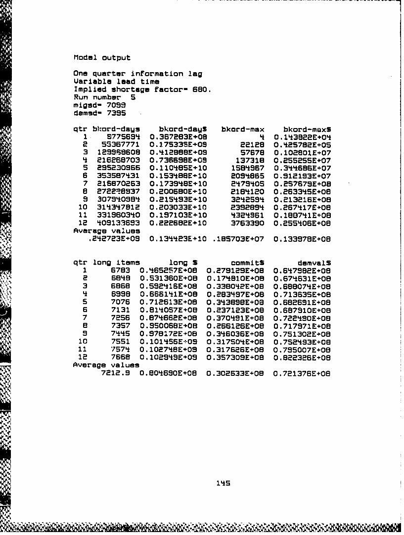
Model output
One quarter information lagUariable lead timeImplied shortage factor- 660.Run number 5migsd- 7099demsd- 7395
qtr bkord-days bkord-day$ bkord-max bkord-mux$1 S77655* 0.367283E+08 4 0.143822E+042 55367771 0.175338E+09 22128 0.425782E÷053 12998608 0.412888E+09 57678 0.102801E+074 216268703 0.736698E+09 137318 0.255255E+075 295230966 0.11048sE+10 1584967 0.344686E÷076 353587431 0.153488E÷10 2094865 0.912193E+077 216670263 0.173488E+10 2479405 0.267679E+088 2722:8937 O.200SOE+10 2184120 O.263345E+089 307940984 0.215493E+10 3242S94 0.213216E+08
10 314347812 0.203033E+10 239289L O.267417E40811 331960340 0.197103E+10 4324961 0.180741E+0812 409133693 0.222682E+10 3763390 O.2SSS06E+08
Average values.242723E+09 0.134423E+10 .185703E+07 0.133978E+08
qtr long items long S commits demvalS1 6783 0.E66257E÷08 0.279129E+08 0.657982E+082 6688 0.531360E+08 0.17810E+08 0.674631E+083 6868 0.592416E+08 0.338042E÷08 0.688074E+08Lf 6998 0.666141E08 0.2B3497E+08 0.713635E+08
5 7076 0.712613E+08 0.343898E+08 0.682631E+086 7131 0.814007E+08 0.237123E+08 0.687910E+087 7256 O.87'*662E÷08 0.370591E+08 0.722490E+088 7357 0.950068E+0B 0.266126E+08 0.717971E+089 7445 0.978172E+08 0.346036E+08 0.751302E+08
10 7551 0.101'56E-t09 0.317504E+08 0.752'93E+0811 7574 0.102748E+09 0.317626E+08 0.795007E+0812 7668 0.102949E+09 0.357309E+08 0.822326E+08
Average values7212.9 0.804630E+08 0.302633E+08 0.721376E+08
S~155
Appendix C: MIGSIM Output with No Item Migration
"146

Model output, no migration
No information lagConstant lead timeImplied shortage factor- 580.Run number 1migsd- 9905demsd- 7415
Quarter 1 through 12FROM/TO X T P M OUT
X 10800 0 0 0 0T 0 2029 0 0 0P 0 0 822 0 0M 0 0 0 188 0
IN 0 0 0 0 0
qtr bkord-days bkord-dayS bkord-max bkord-maxS1 37 0.S71520E+04 37 0.571520E+042 9 0.202026E+0o4 0.194229E+043 39 0.788550E+04 39 0.796348E+044 10 0.370353E+04 10 0.354760E+045 q1 0.104495E+05 *1 0.105S14E+÷06 10 0.508932E+0 10 0.499167E+047 40 0.729216E+04 40 0.729216E+04a 12 0.213670E+04 12 0.213670E+049 10 0.411047E+04 10 0.411847E+04
10 3 0.2q8B97E+04 3 0.248897E+0411 1 0.162409E+04 1 0.162*09E+0O12 3 0.172983E+04 3 0.172983E+04
Average values.179167E+02 0.452113E+04 .179167E+02 0.450849E+04
qtr long items long S commits demval$1 6380 0.289579E+08 0.225930E+09 0.664603E+082 6329 0.286041E+08 0.847471E+07 0.664603E+083 6281 0.282801E+08 0.217126E+08 0.664603E+08I 6234 0.279866E+08 0.897619E+07 0.664603E+085 6193 0.277307E+08 0.222510E+08 0.664603E+086 6169 0.27*566E+08 0.977319E+07 0.664603E+087 6142 0.272180E+08 0.225183E+08 0.664603E÷088 6113 0.270024E+08 0.996617E+07 0.664603E+089 6080 0.268043E+08 0.229681E÷08 0.664603E+08
10 6049 0.26615E+÷08 0.972604E+07 0.664603E+0811 6027 0.264359E+08 0.227223E+08 0.664603E+0812 6011 0.262622E+08 0.100716E+08 0.664603E+08
Average values6167.8 0.274443E+08 0.159794E+08 0.664603E+08
147
Appendix D: MIOSIM Output with Altered-Transition Matrix
i148
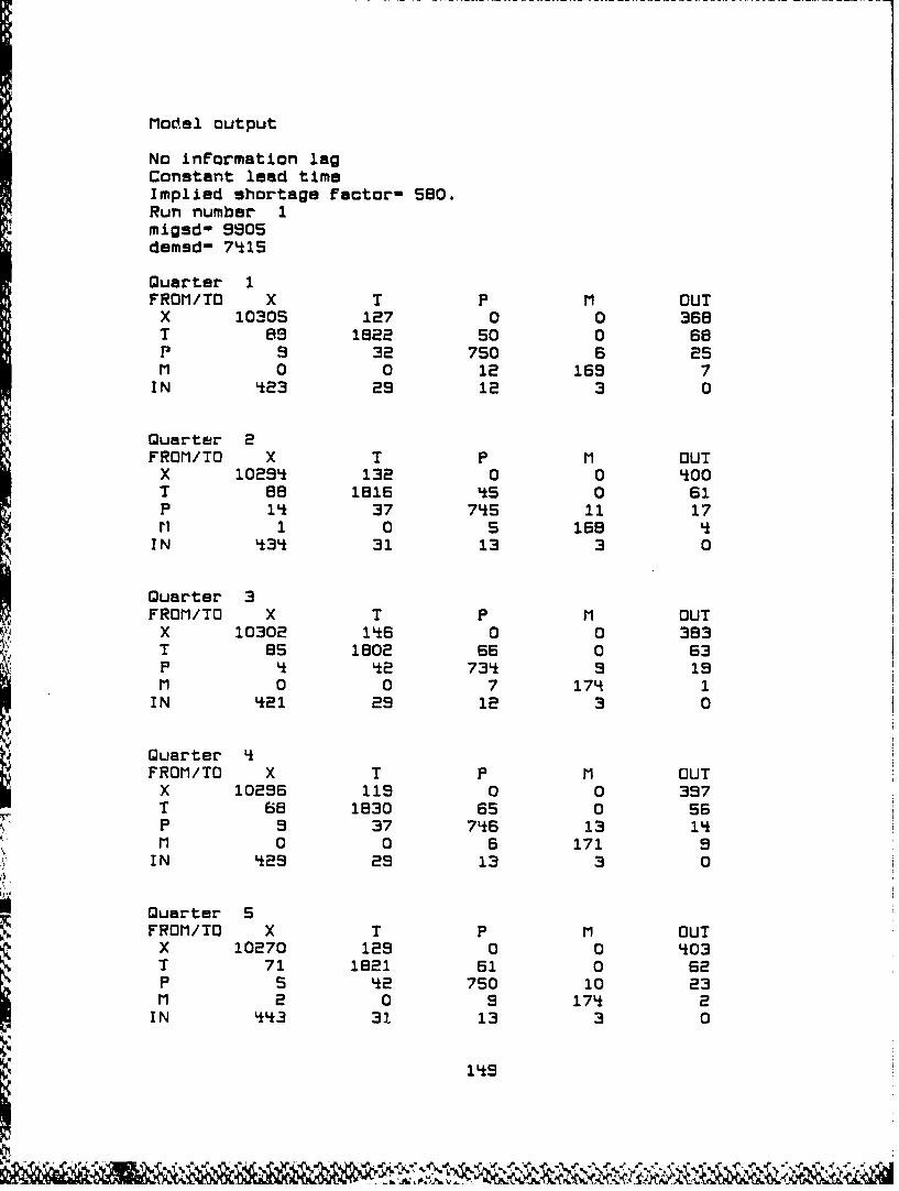
Model output
No information lagConstant lead timeImplied shortage factor- 580.Run number 1migsd- 9905demsd- 741S
Quarter IFROM/TO X T P M OUT
X 1030S 127 0 0 368T 89 1822 so 0 68P 9 32 7S0 6 25M 0 0 12 165 7
IN 423 29 12 3 0
Quarter 2FROM/TO X T P M OUT
X 10294 132 0 0 400T 88 1816 45 0 61P 1'k 37 745 11 17P1 1 0 5 165 4
IN 434 31 13 3 0
Quarter 3FROM/TO X T P M OUT
X 10302 146 0 0 383T 85 1802 66 0 63P Lk 42 734 9 19M 0 0 7 174 1
IN 421 29 12 3 0
Quarter 4FROM/TO X T P M OUT
X 10296 119 0 0 397T 68 1830 65 0 56P 9 37 746 13 14M 0 0 6 171 9
IN 429 29 13 3 0
Quarter 5FROM/TO X T P M OUT
X 10270 129 0 0 403T 71 1821 61 0 62P S 42 750 10 23M 2 0 9 174 2
IN 443 31 13 3 0
149
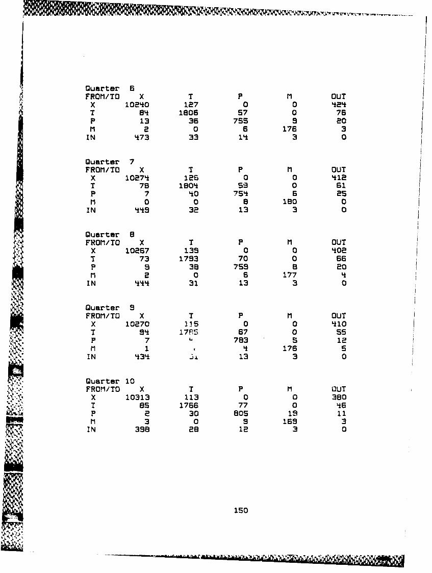
Quarter 6FROM/TO X T P M OUT
X 10240 127 0 0 424T 54 1806 57 0 76P 13 36 75S 9 20M 2 0 6 176 3
IN 473 33 14 3 0
Quarter 7FROM/TO X I P p OUT
X 10274 126 0 0 412
T 7B 1804 53 0 61P 7 40 754 6 25M 0 0 a 180 0
IN 449 32 13 3 0
Quarter 8FROM/TO X T P M OUT
X 10267 139 0 0 4*02T 73 1783 70 0 66P 9 38 759 8 20M 2 0 6 177 4
IN 444 31 13 3 0
Quarter 9FROM/TO X T P M OUT
X 10270 115 0 0 4 10T 94 17F5 67 0 55
_,_ Pat7 7B3 5 12SM 1 , 176 s,K'IN 434 3 13 3 0
• Quarter 10
FROM/TO X T P M OUTSX 10313 113 0 0 380- T es 1766 77 0 46
' P 2 30 805 is 11
--- 3 0 9 168 3SIN 398 28 12 3 0
•.• 150
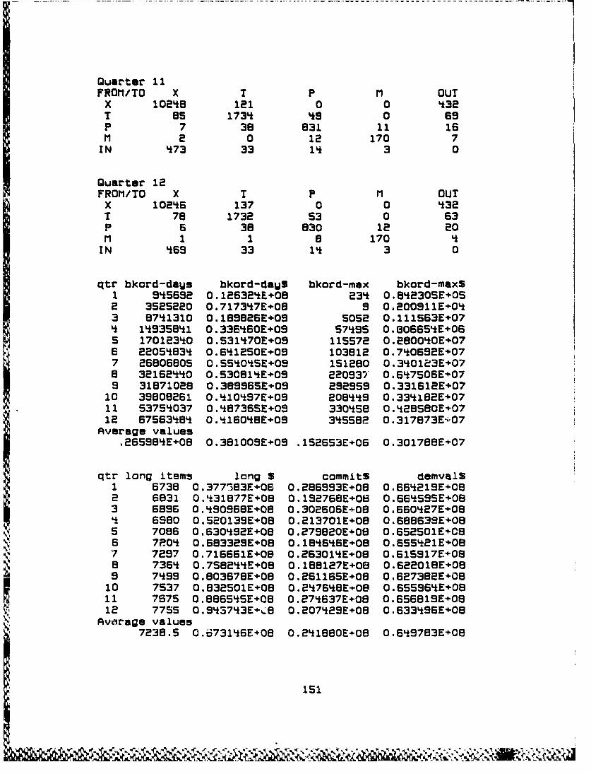
Quarter 11FROM/TO X T P M OUT
x 10248 121 0 0 432T 85 1734 49 0 69P 7 36 831 11 16M 2 0 12 170 7
IN 473 33 14 3 0
Quarter 12FROM/TO X T P M OUT
X 10246 137 0 0 432T 78 1732 53 0 63P 6 38 830 12 20M 1 1 8 170 4
IN 469 33 14 3 0
qtr bkord-daUs bkord-dauS bkord-max bkord-maxS1 9S5692 0.12632SE+08 234 0.842305EOS2 3525220 0.717347E+08 9 0.200911E÷043 8741310 0.189826E+09 5052 0.111563E+07S 14935841 0.336S60E+09 57495 0.5065StE÷065 17012340 0.531470E09 115572 0.2800402E076 22054834 O.6S1250E+09 103812 0.7St092E2077 26805805 C.655*0SE+09 151280 0.340123E2078 32162440 0.530814E÷09 220937 0.647506÷E079 31871028 0.389955E÷09 292959 0.331612E207
10 39808261 0.410497E+09 208449 0.334182E+0711 53754037 0.S87365E+09 3304StB O.'8580E+0712 67553484 0.416048E+09 3S5582 0.317873E2-07
Average values.265984E+08 0.381009E09 l52653E+06 0.301788E+07
qtr long items long S commit$ demvalS1 6738 0.377863E+06 0.286993E+08 0.664219E+082 6831 0.431877E+08 0.192756E+08 0.669SSS5E083 6896 0.490968E+08 0.302606E+08 0.660427E+08S 6980 0.520139E+08 0.213701E+08 0.688639E+085 7086 0.630492E+08 0.279820E+08 0.552501E2C96 7P04 0.683329E+08 0.184646E+08 0.6S5521E2087 7297 0.716661E+08 0.263014E+08 0.615917E÷088 7364 0.7582'*E+08 0.1881272+08 0.622018E2089 7t99 0.803678E+08 0.261165E+08 0.627382E+08
10 7537 0.832501E+08 0.2S7648E*08 0.655964E÷0811 7675 0.886545E+08 0.274637E+08 0.656819B+0812 7755 0.9St743E2+..8 0.207t29E+08 0.633496E+08
Average values7238.5 0.673146E+08 0.241880E+08 O.6S9783E+O8
151

Model output
No information lagConstant lead timeImplied shortage rector- 580.Run number 2migud- 6057demad- 2873
Quarter 1FROM/TO X T P M OUT
X 10270 132 0 0 398T 91 1822 51 0 65P 7 33 754 12 16M 0 0 6 177 5
IN L37 31 13 3 0
Quarter 2FROM/TO X T P M OUT
X 1029o 1i5 0 0 401T 91 1807 55 0 55P 8 35 763 7 11M 0 0 6 180 6
IN Lt27 29 13 3 0
Quarter 3
FROM/TO X T P M OUTX 10322 127 0. 0 376T so 1775 s8 0 53P s 39 774 9 20
M 1 011 0 0 I39IN 109 29 12 3 0
QuarterFROM/TO X T P M OUT
X 10308 ill 0 0 388T 73 1775 55 0 67P 7 39 787 9 20M 1 0 6 179 3
IN 441 31 13 3 0
Quarter 5FROM/TO X T P M OUT
X 10303 127 0 0 400
T 61 1778 59 0 58P 11 39 782 11 18M 1 0 8 174 B
IN 437 31 13 3 0
152

-- -_ _ _ -~- --------- ~ iW 'V 1 ~ ~ V V ~ uw~
Quarter 6FROM/TO X T P M OUT
X 10305 138 0 0 370T 77 1761 67 0 70P 7 '6 777 12 20M 1 1 6 175 S
IN '19 29 12 3 0
Quarter 7FROM/TO X T P M OUT
X 10273 126 0 0 410T 75 1793 58 0 Li9P 10 30 789 12 21M 0 0 4 182
IN *37 31 13 3 0
Quarter 8FROM/TO X T P M OUT
X 10246 137 0 0 '12T 81 1779 50 0 70P 15 34 778 17 20M 1 0 6 183 7
IN *59 32 1'* 3 0
Quarter 9FROM/TO X T P M OUT
X 10255 113 0 0 434T 79 1781 50 0 72F 3 16 770 10 19M 3 1 6 185
IN 482 34 14 3 0
Quarter 10FROM/TO X T P M OUT
X 10242 144 0 0 '36T 61780 46 0 53P a 3S 766 9 22M 1 0 9 185 3
IN 464 33 14 3 0
153
"SiI-
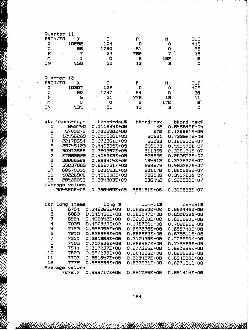
Quarter 11FRO?1/TO X - P M OUT
X 10292 104 0 0 '1isT 86 1790 51 0 65P 7 33 769 7 19M 1 0 6 182 a
IN 458 32 13 3 0
Quarter 12FROM/TO X 7 P M OUT
X 10307 132 0 0 405T o0 1747 64 0 58P 5 31 :776 16 11M 0 0 8 178 6
IN '*3'* 31 13 3 0
qtr bkord-das bkord-dayS bkord-max bkord-maxS1 843740 0.111294E+08 'k2 0.6i56'6E+042 4703575 0.789890E+0B 272 0.132281E+063 12'4S6269 0.200326E+09 20891 0.73952•!+06'* 22178654 0.373961E+09 66983 0.120933E+07S 2574t123 0.440309E÷09 206173 0.4L!147BE+U76 30376992 0.380397E+09 211365 0.369124E+077 273896a9 0.402363E+09 279266 0,263537E÷078 38866585 0.S53414E+09 19'813 0.333837E+079 55037065 0.692731F+09 289974 0.493757E+07
10 68570351 0.688143E*09 601178 0.620585E+0711 50226906 0.431206E+09 786048 0.341725E+0712 28426053 0.384803E+09 5364q2 0.528580E+07
Average values.•30'520E+08 0.396489E+09 .266121E+06 0.300532E+07
qtr long items long S commrits demvalSI 675q 0.348265E+03 O.--2esOE+O8 0.689445E+082 6863 0.34S56SE+08 0.165047E+08 0.69083SE+083 652q 0.40EH2'E+08 0.321020E+08 0.699080E+064 7039 0.460880E+08 0.178733E+06 0.702621E+085 7123 0.585058E+08 0.297278E÷08 0.665740E+086 7210 0.629959E+08 0.226293E408 O.673S11E+087 7311 O.661986E+08 0.317'k38E+0B 0.J02960E+088 740S 0.707538E+08 0.228567E+08 0.71SS23E+089 7544 0.817237E+08 0.277354E+08 O.68D56SE+0O
10 7623 0.860339E+08 0.204825E+08 O.6ESS9E+0811 7707 0.861647E+08 0.238427E+08 0.65499H8E*0812 7772 0.959286E+08 0.237031E+08 0.627131E+06
Average values7272.7 0.636717E+0O 0.2S1725E+06 0.681414E+08
S154
'Vký,

Model output
No information lagConstant lead timeImplied shortage factor- 580.
Run number 3migsd- 9745demsd- 3447
Quarter 1FROM/TO X T P M 011T
X 10278 128 0 0 i9•T 87 1836 Li8 0 57P 6 30 761 S 20I 0 0 7 -..175 5
IN '28 28 13 3 0
Quarter 2FROM/TO X T P M OUT
X 10275 116 0 0 408T 81 1831 59 0 49P 8 37 768 3 i4M 0 0 13 168 2
IN 428 28 13 3 0
Quarter 3FROM/TO X T P M OUT
X 10253 121 0 0 *21T 77 1808 67 0 61P 10 35 776 7 25M 0 0 ) 161 6
IN 463 33 14 3 0
Quarter L
FROM/TO X T P M OUTX 10276 120 0 0 407T 85 1787 50 0 65P 11 37 786 9 P2M 2 0 8 158 3
IN 114 8 32 13 3 0
Quarter 5FROM/TO X T P M OUT
X 10330 113 0 0 380T 86 1775 52 0 53P 8 33 780 1e A8M 0 0 10 152 8
IN 424 29 12 3 0
155
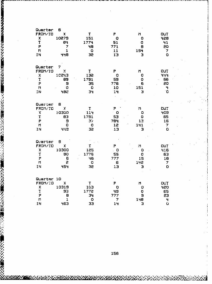
Quarter 6FROM/TO X T P M OUT
X 10279 151 0 0 428T 8~k 177'* 51 0 '* 1P 7 48 771 B 20M 1 0 11 154 7
IN 448 32 f3 3 0
Quarter 7FROM/TO x T P M OUTx IC103 132 00I~~
T 89 1791 59 0 66P 9 35 776 6 20M 0 0 10 151
IN 4B2 34 14 3 .0
Quarter 8FROM/TO X T P M OUT
X 10300 lII 0 0 409T 83 1791 53 0 65P 9 3' 784 12 16"M 0 0 12 141 7
IN Yfk9 32 13 3 0
Quarter 9FROM/TO X T P M OUTX 10300 125 .0 0 416
T 80 1776 55 0 63P 6 '*6 777 is 1eM 2 06 142 7
IN 455 32 13 3 0
Quarter 10FROM/1'O X T PM OUT •
X 10319 103 0 0 420
T 93 1776 59 0 65P 8 32 777 9 23M 1 0 7 i48
IN 463 33 i4 3 U
156
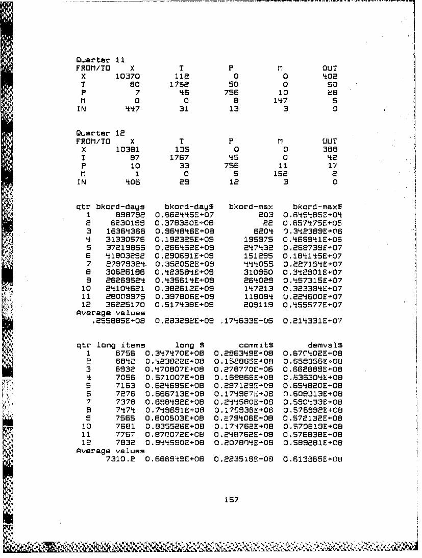
Quarter 11FROM/TO X T P r OUT
X 10370 112 0 0 402T 80 1752 so 0 50P 7 46 756 10 28M 0 0 8 147 S
IN L*5f7 31 13 3 0
Quarter 12FROM/TO X T P M OUT
X 10381 135 0 0 388T 87 1767 45 0 42P 10 33 756 11 17M 1 0 5 152 2
IN 406 29 12 3 0
qtr bkord-dags bkord-daWS bkord-max bkord-maxS1 898792 0.6624455+07 203 0.56655Z4+042 6230199 0.378360E-08 22 O.657475E÷053 16364366 0.964846E+08 6204 0.3q2389E+064 31330576 0.192325E+09 195975 0.I*669L1E+065 37219855 0.266452E+09 247432 0.268739E+076 41803292 0.290681E+09 151295 0.18l1i5E+077 27979324. 0.352052E+03 444055 0.22715IE+078 30626186 0.2358'*E+09 310950 0,3i2901E+079 26269524 0.435614E4+09 26*029 0."57315E+0710 24104621 0.382612E+09 147213 0.323304E+0711 28009975 0.3978O6E+09 119094 0.224600E+0712 36225170 0.517438E+09 209119 0.555577E+07Average values
.255885E+08 0.283292E+09 .174633E+05 0.214331E÷07
qtr long items long S commits demval$1 6756 0.347470E+08 0.286349E408 0.670C02E+082 6862 0.Li23822E408 0.1S286SE+0H 0.658356E+083 6932 0.470807E+08 0.278770E+06 0.662889E+08I 7056 0.571007E+08 0.169866E+0B 0.636304E+085 7163 0.624695E+08 0.287129E+08 0.6S4820E+08
"V 6 7276 0.666713E+08 0.17i9E7Lo+8 n.608313E+087 7378 0.698492E+08 0.244580E+08 0.590433E+088 7474 0.749691E+08 0.176936E+06 0.576992E+089 7565 0.800503E+08 0.79S406E+08 0.572132E+08
10 7681 0.835526E+08 0.174762E+08 0.570819E+0811 7767 0.870072E+06 0.248762E+08 0.576838E+0812 7832 0.9485550Z+08 0.207804.E+08 0.589281E÷08
Average values7310.2 0.666•SE+08 0.223516E+08 0.613365E+08
157

model output
No information lag.Constant lead timeImplied shortage factor- 580.Run number 4migsd- 1075demsd- 1175
Quarter 1FROM/TO X T P OUr
X 10262 120 0 0 418T 82 1830 57 0 soP S Li 74*9 15M 3 0 13 1i8 3
IN 448 32 13 3 0
Quarter 2FROM/TO X T P M OUT
X 10280 116 0 0 404T s0 1822 58 0 56P _ 2a 762 6 32N 0 0 8 165 7
IN Lisi 32 13 3 0
Quarter 3FROM/TO X T P M OUT
X 10260 133 0 0 432T 8L 1806 Lie '0 56P 6 52 755 13 161M 2 0 8 157 6
IN LiSi 3E 12 3 0
Quarter LFROM/TO X T P M OUT
X 10271 113 0 0 433T 81 1802 58 0 72P 4 Lis 751 6 20M 0 2 5 161 5
IN 473 34 1iLt 3 0
Quarter 5FROM/TO X T P M OUT10291 131 0 0 413
97 1770 se 0 718 36 765 10 19
M 0 8 157 5
IN '*59 32 13 3 0
15I

Quarter 6FROM/TO X T P M OUT
x 10282 137 0 0 438T so 1773 47 0 59F 6 36 764 13 23M 0 0 7 160 3
IN 473 33 14 3 0
Quarter 7FROM/TO X T P M OUT
X 10333 136 0 0 382T 76 1788 60 0 55P 8 35 754 20 1iM 0 0 8 164 L
IN 412 29 12 3 0
Quarter 8FROM/TO X T P M OUT
X 10266 123 0 0 440T 80 1791 57 0 60P 8 37 756 12 21M 1 0 8 170 8
IN 478 34 11* 3 0
Quarter 9FROM/TO X T P M OUT
X 10298 121 0 0 414T 81 1793 60 0 51P 7 47 74 1 16 24M 0 0 9 172 L
IN *'' 31 13 3 0
Quarter 10FROM/TO X T P M OUT
X 10304 108 0 0 418IT 94 1780 59 0 59P 7 43 744 5 24M 0 0 9 174 8
IN 459 32 1'* 3 0
159
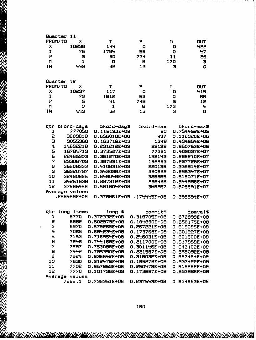
Quarter 11FROM/TO X T P M OUTX 10298 144~ 0 0 2T 76 17B4k 56 0 4*7P 5 so 734* 11 26M 1 0 a 170 3
IN 449 32 13 3 0
Quarter 12FROM/TO X T P M O1IIx 10297 117 0 0 4*151 79 1812 53 0 66p 5 '*1 74*8 S 12ri 0 1 6 173 LIN 44'9 32 13 3 0
qtr bkord-days bkord-daWS bkord-max bkord-maxS1 7770S60O.116193E+08 60 O.7S44S*2E+052 3609818 0.656018E+08 '*87 0.116920E+063 9055960 0.163718E+09 134*9 O.'*94*65'E+06'* 14*692218 0.291212E+09 95199 0.850753E4-065 1678'*719 0.373527E+09 77391 0.4*09097E+076 22'*6S903 0.361270E+09 13214*3 0.288210E+077 29306709 0.387891E+09 186283 0.297726E+078 36508933 0.4*10831E+09 220136 0.339814*E+079 36920797 0.54*9096E+09 380692 0.28634*7E+07
10 324*90895 0.64*9048BE+09 326865 0.519071E+'0711 34*251636 0.697912E+09 296'*6B 0.644'996E+0712 372854*56 0.561804*E+03 3b6267 0.609291E+07Average values
.2284*56E+'08 0.376961E+09 .17444*'5E+06 0.295694*E+07
qtr long items long S commit$ demvalS1 6770 0.372332E+08 0.318705E+08 0.672899E+082 6862 0.502979E+08 0.18'i890E+08 0.656175E+083 6970 0.579269E+08 0.267221E+08 0.519095E+08
4 706S 0.684*234*E+08 0.173768E+08 0.601227E+085 7153 0.716954*E+08 0.24*6031E+08 0.601500E+086 724*6 0.744P168E+08 0 .211700E+01B 0.617959E+.087 7287 0.753089E+08 0.3011'*6E+08 0.6'*2'02E+-088 744'2 0.795350E+08 0.221537E+013 0.669092E+089 7524* 0.8355'k2E+08 0.316032E+'08 0.6874*24E+0810 7630 0.3124*76E+06 0.18527BE+08 0.6374*22E+0811 7702 0.9S7859E+08 0.2504k79E+08 0.616292E+08
Average values
7285.1 0.739351E+08 0.2375'*3E+08 0.634*623E+08
160

Model output
No information lagConstant lead timeImplied shortage factor- 560.Run numier 5migad- 7099demsd- 7395
Quarter 1FROM/TO X T P M OUT
X 10203 139 0 0 '58T 82 1815 74 0 56P 8 3S 756 5 18M 1 1 7 174 S
IN 4187 34 14 3 0
Quarter 2FROM/TO X T P M OUT
X 10224 125 0 0 432T 86 1811 62 0 65P 12 38 764 12 25M 0 1 6 167 8
IN 479 34 14 3 0
Quarter 3FROM/TO X T P M OUT" " 10264 134 0 0 403
T 63 1817 61 0 68P 7 43 770 8 18M 1 0 S 175 1IN 443 31 13 3 0
Quarter 4FROM/TO X T P M OUT
X 10216 142 0 0 420T 77 1818 61 0 689P a 42 774 E isM 1 0 7 169 9
IN 467 33 14 3 0
Quarter 5FROM/TO X T P M OUT
X 10184 135 0 0 450T 91 1833 so 0 SiP 11 28 787 B 22M 2 0 7 164 5
IN 477 34 14 3 0
161
~AtVAAA PL1A~L W~& A- ý1 kA~ -"i .. i 1 .1 VAA

Quarter 6FROM/TO X T P M OUT
X 10231 129 0 0 405T 100 1834 43 0 53P 14 30 793 8 23M 1 1 6 163 4
IN L138 31 13 3 0
Quarter 7FROM/TO X T P M OUT
X 10226 133 0 0 '25T 95 1827 57 0 '*6P 7 33 781 12 22M 2 1 4 161 6
IN 451 32 13 3 0
Quarter 8FROM/TO X T P M OUT
X 10208 138 0 0 '3ST 88 1810 61 0 67P 10 39 780 8 lBM 0 0 B 164 '
IN 473 33 1'* 3 0
Quarter 9FROM/TO X T P M OUT
X 1023S 127 0 0 417T 86 1811 51 0 62P 7 31 794 9 22M 0 0 4 164 7
IN Li5s 32 13 3 0
Quarter 10FROM/TO X T P M OUT
X 10252 101 0 0 445T 70 1e08 52 0 71P 4 38 801 6 13M 1 0 4 166 5
iN 482 34 1'* 3 0
162

Quarter 11FROM/TO X T P M OUT
X 10272 125 0 0 412T 82 1780 50 .0 69P 8 34 801 6 22M 1 0 7 163 t
IN 458 32 13 3 0
Quarter 12FROM/TO X T P M OUT
X 10250 133 0 0 438T 92 1770 55 0 54P 13 45 783 15 15M 0 0 8 157 7
IN 464 33 14 3 0
qtr bkord-days bkord-daWS bkord-max bkord-maxS1 148S959 0.199849E+08 37 0.555608E÷04
2 9723043 0.105411E+OS 359 0.103793E063 23876663 0.269367E+09 48909 0.921749E+06Lt 3555918* 0.411866E÷09 235774 0.200822E+07S 35870655 0.SS5598E+09 287824 0.357920E+07S 32094609 0.599'20E+09 208744 0.485505E+077 28304119 0.8a56*0E÷09 354933 0.688712E+078 22227702 0.336574E+09 150069 0.272196E÷079 24696686 0.35*556E+09 183663 0.299757E+07
10 28261902 0.384840E+09 142946 0.291554E+0711 30S71644 0.414526E+09 466498 0.368B14E+0712 22706904 0.355353E+09 138311 0.353407E+07
Average values.246152E+00 0.357761E+09 .184839E+06 0.285149E+07
qtr long items long S commits demvalS1 6781 0.345923E+08 0.324289E+08 0.689508E+082 6879 0.392488E+08 0.187215E÷08 0.710893E+083 6954 0.'75747E+08 0.331402E+08 0.689218E+08t 7077 0.525031E+08 0.157839E+08 0.692056E+085 7209 0.570918E+08 0.285360E+08 0.654399E+086 7284 0.612844E+08 0.165965E÷08 0.6457'6E÷087 7418 0.651551E+06 0.298128E÷08 0.656762E+08B 7528 0.698415E+08 0.183935E+08 0.631996E÷089 7592 0.720133E+08 0.286491E+08 0.647411E+08
10 7683 0.746994E+08 0.1873S7E÷08 0.6'*8791E+0811 7756 0.835592E+06 0.24'510E+08 0.606463E+0812 7859 0.867711E+08 0.239329E+08 0.638898E+08
Average values7335.0 0.620201E+08 0.240985E+08 0.6593'SE+08
163
S.w.

Appen~dix E: SAS Residual Plots
I l 1
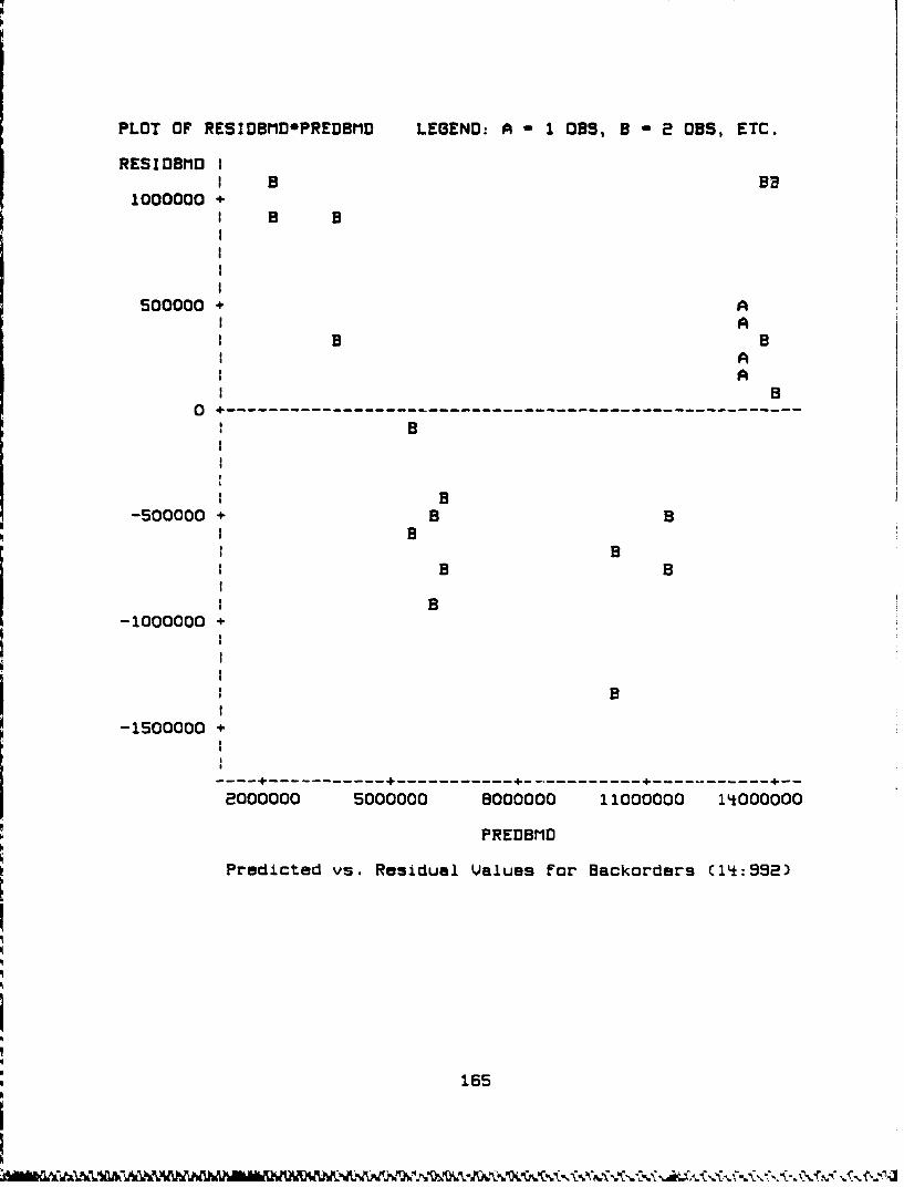
PLOT OF RESIDBMDOPREDBMD LEGEND: A - 1 OBS, B - OBS, ETC.
RESIDBMD II B BE
1000000 +I B B
500000 + AA
B BAA
B0 --------------------------------------------------------
B
B-500000 + B B
IB* B
B BB
-1000000 +
I B
-1500000 +B
-1500000 500~0000 OOO 1100~0000 1'k000000
Predicted vs. Residual V.alues for- Backorders (1t*:932)
165

PLOT OF BMDRANKORESIOBMD LEGEND: A 1 0BS, B - 2 OBS,ETC.
2.0 A
R AA 1.5 + AN I
X Z AI A
F 1.0+ AA0 AOI A
R
AU 0.5 + A A
A BR A AA1 A A
A 0.0 + A A
B A AL A A
E AA-0.5 + AA
R AE BS A1 -1.0 +* B
B A .M
D -1.5 + AA A
-2.0 + A
------ --.------------- ---- -- -.----
- SO0000 -lOCO000 -500000 0 S00000 1000000
RESIDIDBM
Ranked Residual Plot For Backorders C15:64B)
166
Nk, M

PLOT OF RESIDLSDOPREDLSD LEGENU: A - 1 0BS, 5 2 OBS, ETC.
RESIDLSD 1
1200000 +AA -
AA
S500000 +
SA600000 + A
A A AI A300000 + A A
A A AA A A
I A0 -- - - A -- - - - - - - - - - - - -A--A--A ------- R---
SAA A AS: AA A
I i A A A
-300000 +
S~A
-600000 + AS~A
-900000 +
h :A At -1200000 + A
- - ---------- 4 -------------- 4------------------- +---------------- --- -- -- -
66000000 70000000 74000000 76000000 82000000 86000000
PREDLSU
Predicted vs. Residual Ualues For Long Supply (14:992)
167
Ril
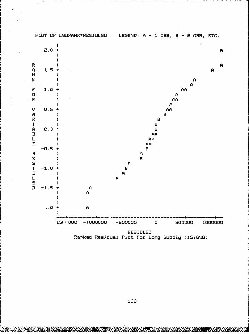
PLOT OF LSURANKORESIDLSD LEGEND: A I 1 OBS, B - 2 0BS, ETC.
2.0 + A
R A
. I.: + ANI
K IA
AAA
I A
-01.5 + B•
R AA
A BR a
I -. 0 BB AAL IAASF AA
-0.5 + BR i AE i BS i A1 -1.0 + B
AAL IASI0 -1.5 + A
.. 0 + A
RESIDLSORanked Residual Plot For Long Supply (15:648)
168
Biblicaraph,
1. Pir Force Logistics Command. Requirements ProceduresFor Economic Order Quantitu (EOQ) Items. AFLCR 57-6.Wright-Patterson AFB OH: Headquarters Air ForceLogistics Command, 22 August 198'.
2. Bagchi, Uttareyan et al. "Concepts, Theory, andTechnique: Modeling Demand During Lead-Time."Decision Sciences, 1S: 157-176 (Spring 19l8).
3. Blazer, Maj Douglas J. "Variability of Demand: Whythe Part is Never on the Shelf." Air Force Journalof Logistics, 9: 11-13+ (Spring 1985).
k. Casey, Donald L. Item Migration. Working Paper
No. XRS84-21S-4. Directorate of ManagemsntScience, OCS/PLans and Programs, HeadquartersAir Force Logistics Command, Wright-PattersonAFB OH, August 1986.
S. Cohen, Morris A. et al. "Optimal Stockage Policies ForLow Usage Items in Multi-Echelon Inventory Systems."Naval Research Logistics Quarterlu, 33: 17-38(February 1986).
6. Demmy, W. Steven. "A Study to Develop Improved EOQInventory Management Policies: -Final Report."Contract F33000-80-C-0530. Decision Systems,Beavercreek OH, March 1982 (AD-A12*547).
7. Demmy, W Steven. "The Inventory System Simulator(INSSIM), Uolume 1: Model Description." ContractF49620-77-C-O063. Decision Systems, Beavercreek OH,August 1977.
B. Demmy, W. Steven and Gloria J. Picciano. "InventoryManagement Research: Some Recent Findings and NewDirections For the iSBOs." Report, HQ Air ForceLogistics Command, Wright-Patterson AFB OH, undated.
9. Disz, Thomas E. An Evaluation of the Effect of
Establishina a Minimum Economic Order Quantitu (EDO)on the Air Force EOQ Item Management SUstem. MS ThesisAF.T/GLM/LSM/84S-14. School of Systems and Logistics,Air Force Institute oF Technology (AU), Wright-Patterson AFB OH, 1984
169

10. Hobson, Jeffrey J. and Ronald A. KirchcfC. An appli-cation of Markov Chains to the Problem of Migrationin Inventoru Sustems. MS Thesis AFIT/GOR/OS/84D3-6.
FSchool of Engineering, Air Force Institute ofTechnology (AU), Wright-Patterson AFB OH, 1984.
11. Kennedy, John D. The Impact of Item Migration in theAir• Force ._Lpistics Command Consumables Inventoru.
,, MS Thesis AFIT/GOR/OS/BSD-11. School of Engineering,Air Corce Institute of Technology (AU), Wright-Patterson AFB OX, 1984'.
12. Lowe, Timothy J. ard Leroy B. Schwarz. "ParameterEstimation for the EO Lot-Size Model: Minimax andExpected Valua Cthoices." Naval Resear-ch LogisticsQuarteclq, 3;20: 357-376 (June 1883).
13. Prasutti, V.4ctor J., Jr. and Richard C. Trepp. "MoreAdo About Economic Order Quantities (EDOQ)." NavalRs~seqrch Logistics Duarteriu, 17: 2*3-2S1 (June 1870).
14. SAS institute Inc. SAS User's Guide: Basics, Uersion 5Edition. Cary NC: SAS Institute Inc. 1895.
15. SAS Institute Inc. SAS User's Guide: Statistics,Uersion 5 Edition. Cary NC: SAS Institute Inc. 1885.
16. Smith, Kevin P. Estimation of Inventory Item DemandDistributions: Modeling Iten Migration at the DefenseElectronics Supplu Center. MS ThesisAFIT/GOR/OS/85D-11. School of Engineering, Air ForceInstitute of Technology (AU), Wright-PattersonAFB OH, 1i84.
17. Smith, Palmer W., Operations Research Analyst.Persona: interview. BDM Corp, Kettering OH,12 November 1886.
18. Smith, Lt Col Palmer W. and Robert Gumbert. "ItemMigration and the Dynamics of Inventory Management."Defense Management Journal, 22: 3-11(First Quarter 1S86)
18. Ward, J. B. "Determining Reorder Points When Demandis Lumpy." Management Science, 2q: 623-632(February 1978).
170
UiTA
Lee J. Lahmkuhl was born on 15 November 1958 in Sumner,
Iowa. He graduated from high school as valedictorian in
Davenport, Iowa, in 1977. He graduated From the University
of Iowa in May IBe, receiving a Bachelor of Science ,iegree
in Mathematics. As an Air Force RDTr Distinguished
Graduate, he received a commission in the USAF and reporteN
For active dutq in October 1981 at the Air Force Electronic
Warfare Center (AFEWC), San Antonio, Texas. While at the
AFEWC, he servud as .a scientific analyst in simulation'
validation and glectronic combat eFfectiveness; andas
Commander, Squadron Section. He entered the School of
Engineering, Air Force Institute of Technology,
in May 1s85.
Permanent address: R.R. 1, Box q01
LeClaire IA 527S3
171