AFM image reconstruction for deformation measurements by digital image correlation

This article has been downloaded from IOPscience. Please scroll down to see the full text article.

2006 Nanotechnology 17 933

(http://iopscience.iop.org/0957-4484/17/4/016)

Download details:

IP Address: 137.99.31.134

The article was downloaded on 18/03/2013 at 19:08

Please note that terms and conditions apply.

View the table of contents for this issue, or go to the journal homepage for more

Home Search Collections Journals About Contact us My IOPscience

INSTITUTE OF PHYSICS PUBLISHING NANOTECHNOLOGY

Nanotechnology 17 (2006) 933–939 doi:10.1088/0957-4484/17/4/016

AFM image reconstruction fordeformation measurements by digitalimage correlationYaofeng Sun1,2 and John H L Pang1

1 School of Mechanical and Aerospace Engineering, Nanyang Technological University,639798, Singapore2 Singapore Institute of Manufacturing Technology, 71 Nanyang Drive, 638075, Singapore

Received 28 November 2005, in final form 16 December 2005Published 30 January 2006Online at stacks.iop.org/Nano/17/933

AbstractThe scanner drift of the atomic force microscope (AFM) is a greatdisadvantage to the application of digital image correlation tomicro/nano-scale deformation measurements. This paper has addressed theimage distortion induced by the scanner drifts and developed a method toreconstruct AFM images for the successful use of AFM image correlation.It presents such a method, that is to generate a corrected image from twocorrelated AFM images scanned at the angle of 0◦ and 90◦ respectively. Theproposed method has been validated by the zero-deformation test. A bucklingtest of a thin plate under AFM has also been demonstrated. The in-planedisplacement field at the centre point of the buckling plate has beensuccessfully characterized by the application of the image correlationtechnique on reconstructed AFM images.

1. Introduction

Digital image correlation [1–3] treating optic images has beenfound to be a popular approach as a full-field displacementmeasurement technique because of the ease of specimenpreparation, experiment operation, and experimental dataprocessing. It is a natural thought to employ the digital imagecorrelation technique to handle AFM images in expectationof nano-scale deformation measurement with the aid ofhigh spatial resolution of AFM. Nano-scale deformationmeasurements are often required to determine strain andmechanical properties of small-sized specimens. With therapid development of micro/nano-fabrication technologies,the characterizations of fabricated micro/nano-structuresare in great demand, which has pushed researchers andengineers to improve or develop experimental mechanicstechniques. Although the AFM image correlation techniquehas attracted increasing attention from the experimentalmechanics community, there are few reports [4, 5] onthe successful application of the AFM image correlationtechnique. One main reason for this is that the scannerdrifts of AFM induce artificial deformation flooding the actualdeformation.

The distortion of AFM images results not only from thenonlinear motions of the AFM piezoelectric scanner whenresponding to the applied voltage, but also from its hysteresisand creep effects, even from the complex cross couplingbetween x , y and z motions. The nonlinearity corrections ofAFMs have been investigated in many studies [6, 7] and provedto be effective in the reduction of the scanner’s nonlinearity. Towhat extent the scanner’s nonlinearity is compensated dependson adopted procedures. In this study a Digital Instruments3000 AFM is used. The nonlinearity of its scanner has beeninvestigated by the digital image correlation (DIC) techniquethat is briefly described in the following section. Basedon the analysis of the characteristics of the nonlinearity, amethod has been developed to remove image distortion and toreconstruct the AFM images. DIC experiments have validatedthe presented method and shown that it is practical to usereconstructed images for deformation measurement by DIC.

2. Digital image correlation technique

The digital image correlation (DIC) is applied to obtainthe displacements of the centre point of a subimage on thereference image taken before deformation, when the subimage

0957-4484/06/040933+07$30.00 © 2006 IOP Publishing Ltd Printed in the UK 933

Y Sun and J H L Pang

matches another subimage on the deformed image taken afterdeformation. The match of a subimage is to be found bymaximizing the cross-correlation coefficient between intensitypatterns of two subimages:

C(p) =(

y0+N/2∑y=y0−N/2

x0+M/2∑x=x0−M/2

g(x, y)h(x + u(x, y, p), y + v(x, y, p))

)

×(

y0+N/2∑y=y0−N/2

x0+M/2∑x=x0−M/2

g2(x, y)

y0+N/2∑y=y0−N/2

x0+M/2∑x=x0−M/2

h2(x + u(x, y, p), y + v(x, y, p))

)−1/2

(1)

where the coordinate (x0, y0) represents the centre point of asubimage with its size M × N ; g(x, y) is the light intensity atthe point (x, y) in the reference image; h(x + u(x, y, p), y +v(x, y, p)) is the light intensity in the deformed image at thematch position of the point (x, y). The intensity at a sub-pixelposition is obtained by using a bicubic spline interpolationscheme: I (x, y) = ∑3

n=0

∑3m=0 αmnxm yn. The coefficients

αmn are determined from the intensity values of pixel locations.u(x, y, p) and v(x, y, p) are displacement functions whichdefine how each of the subimage points located in the referenceimage at (x, y) is mapped to the deformed image. First-orderdisplacement functions are often used:

u(x, y, p) = p0 + p2(x − x0) + p4(y − y0)

v(x, y, p) = p1 + p3(x − x0) + p5(y − y0).(2)

The parameter vector p(p0, p1, p2, p3, p4, p5) can be expli-citly denoted p(u(x0, y0), v(x0, y0),

∂u∂x

∣∣x0,y0,∂v∂x

∣∣x0,y0,∂u∂y

∣∣x0,y0,

∂v∂y

∣∣x0,y0) (where u(x0, y0) and v(x0, y0) are the displacementsof the subimage centre in x and y directions respectively).To find the resultant vector p that maximizes the correlationcoefficient (equation (1)), the Newton–Raphson method is usedto iteratively find the solution with a given approximation pold

to the solution. The next improved approximation pnew canbe obtained using the following Newton–Raphson iterationformula:

∇∇C(pold)(pnew − pold) = −∇C(pold). (3)

The Newton–Raphson method is known for its fastconvergence capability. Usually, two or three iterations areenough to solve the parameter vector p, which representsthe displacements and displacement gradients at the subimagecentre. It is practical [8] that the displacement gradientsabove are used for the direct calculation of strain componentsin uniform deformation measurements instead of additionaloperations of displacement field smoothing and derivativecalculation.

In what follows, image correlation results use u torepresent the displacement in the x /horizontal direction of theimages, v in the y/vertical direction of the images.

3. AFM image distortion and reconstruction

The formation of an AFM image is from data collection duringthe scan motion of AFM probe in a type of raster pattern

Fast-scan direction

Slow

-sca

n di

rect

ion

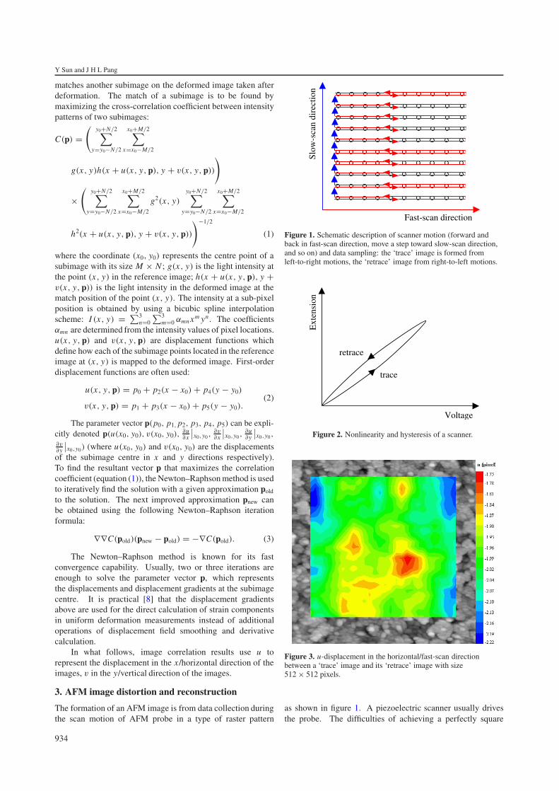
Figure 1. Schematic description of scanner motion (forward andback in fast-scan direction, move a step toward slow-scan direction,and so on) and data sampling: the ‘trace’ image is formed fromleft-to-right motions, the ‘retrace’ image from right-to-left motions.

Voltage

Ext

ensi

on

trace

retrace

Figure 2. Nonlinearity and hysteresis of a scanner.

Figure 3. u-displacement in the horizontal/fast-scan directionbetween a ‘trace’ image and its ‘retrace’ image with size512 × 512 pixels.

as shown in figure 1. A piezoelectric scanner usually drivesthe probe. The difficulties of achieving a perfectly square

934

AFM image reconstruction for deformation measurements by digital image correlation

(a) (b)

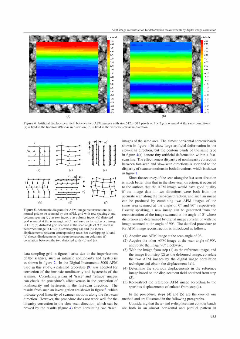
Figure 4. Artificial displacement field between two AFM images with size 512 × 512 pixels or 2 × 2 µm scanned at the same conditions:(a) u field in the horizontal/fast-scan direction, (b) v field in the vertical/slow-scan direction.

rjv

rju

div

diu

t t t t

s s

s

s

j

i

t t t t j

s

s

s

s

i

(a) (c) (e)

(b) (d) (f)

Figure 5. Schematic diagram for AFM image reconstruction: (a)normal grid to be scanned by the AFM, grid with row spacing s andcolumn spacing t, j as row index, i as column index; (b) distortedgrid scanned at the scan angle of 0◦, and used as the reference imagein DIC; (c) distorted grid scanned at the scan angle of 90◦, used asdeformed image in DIC; (d) overlapping (a) and (b) showsdisplacements between corresponding rows; (e) overlapping (a) and(c) shows displacements between corresponding columns; (f)correlation between the two distorted grids (b) and (c).

data-sampling grid in figure 1 arise due to the imperfectionsof the scanner, such as intrinsic nonlinearity and hysteresisas shown in figure 2. In the Digital Instruments 3000 AFMused in this study, a patented procedure [9] was adopted forcorrection of the intrinsic nonlinearity and hysteresis of thescanner. Correlating a pair of ‘trace’ and ‘retrace’ imagescan check the procedure’s effectiveness in the correction ofnonlinearity and hysteresis in the fast-scan direction. Theresults from such an investigation are shown in figure 3, whichindicate good linearity of scanner motions along the fast-scandirection. However, the procedure does not work well for thelinearity correction in the slow-scan direction, which can beproved by the results (figure 4) from correlating two ‘trace’

images of the same area. The almost horizontal contour bandsshown in figure 4(b) show large artificial deformation in theslow-scan direction, but the contour bands of the same typein figure 4(a) denote tiny artificial deformation within a fast-scan line. The effectiveness disparity of nonlinearity correctionbetween fast-scan and slow-scan directions is ascribed to thedisparity of scanner motions in both directions, which is shownin figure 1.

Since the accuracy of the scan along the fast-scan directionis much better than that in the slow-scan direction, it occurredto the authors that the AFM image would have good qualityif the image data in two directions were both from theaccurate scan along the fast-scan direction, and such an imagecan be produced by combining two AFM images of thesame area scanned at the angle of 0◦ and 90◦ respectively.Exactly speaking, a new image can be generated from thereconstruction of the image scanned at the angle of 0◦ whosedistortions are determined by digital image correlation with theimage scanned at the angle of 90◦. The detailed procedure tofor AFM image reconstruction is introduced as follows.

(1) Acquire one AFM image at the scan angle of 0◦.(2) Acquire the other AFM image at the scan angle of 90◦,

and rotate the image 90◦ clockwise.(3) With the image from step (1) as the reference image, and

the image from step (2) as the deformed image, correlatethe two AFM images by the digital image correlationtechnique and obtain the displacement field.

(4) Determine the spurious displacements in the referenceimage based on the displacement field obtained from step(3).

(5) Reconstruct the reference AFM image according to thespurious displacements calculated from step (4).

In the procedure, steps (4) and (5) are the core of ourmethod and are illustrated in the following paragraphs.

Considering that the u- and v-displacement contour bandsare both in an almost horizontal and parallel pattern in

935

Y Sun and J H L Pang

(a) (b)

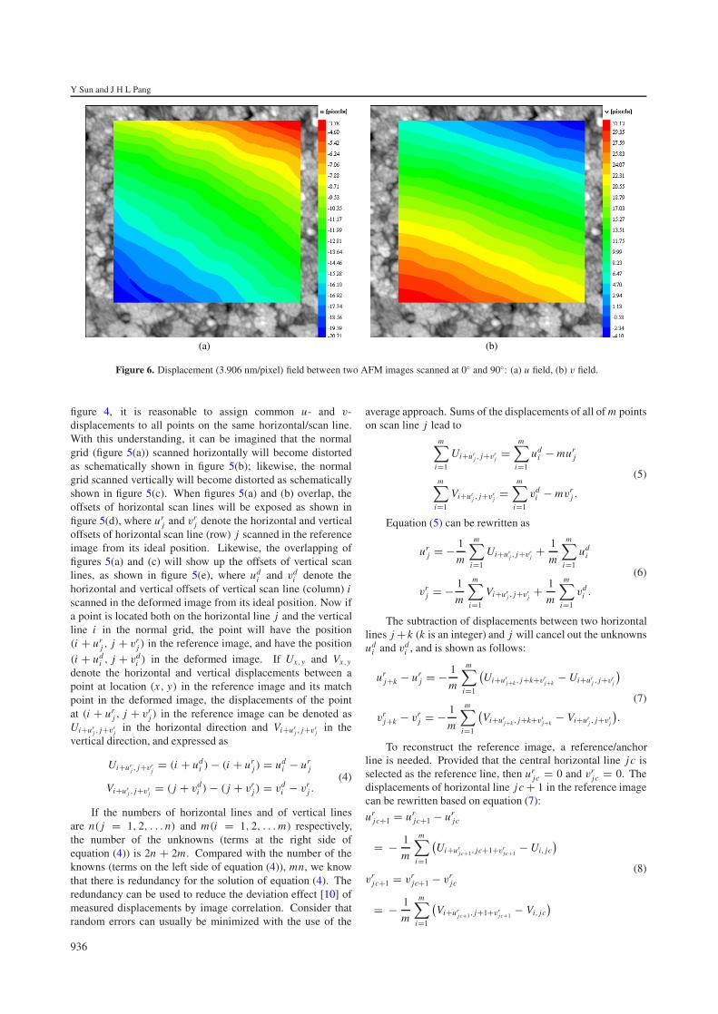
Figure 6. Displacement (3.906 nm/pixel) field between two AFM images scanned at 0◦ and 90◦: (a) u field, (b) v field.

figure 4, it is reasonable to assign common u- and v-displacements to all points on the same horizontal/scan line.With this understanding, it can be imagined that the normalgrid (figure 5(a)) scanned horizontally will become distortedas schematically shown in figure 5(b); likewise, the normalgrid scanned vertically will become distorted as schematicallyshown in figure 5(c). When figures 5(a) and (b) overlap, theoffsets of horizontal scan lines will be exposed as shown infigure 5(d), where ur

j and vrj denote the horizontal and vertical

offsets of horizontal scan line (row) j scanned in the referenceimage from its ideal position. Likewise, the overlapping offigures 5(a) and (c) will show up the offsets of vertical scanlines, as shown in figure 5(e), where ud

i and vdi denote the

horizontal and vertical offsets of vertical scan line (column) iscanned in the deformed image from its ideal position. Now ifa point is located both on the horizontal line j and the verticalline i in the normal grid, the point will have the position(i + ur

j , j + vrj ) in the reference image, and have the position

(i + udi , j + vd

i ) in the deformed image. If Ux,y and Vx,y

denote the horizontal and vertical displacements between apoint at location (x, y) in the reference image and its matchpoint in the deformed image, the displacements of the pointat (i + ur

j , j + vrj ) in the reference image can be denoted as

Ui+urj , j+vr

jin the horizontal direction and Vi+ur

j , j+vrj

in thevertical direction, and expressed as

Ui+urj , j+vr

j= (i + ud

i ) − (i + urj ) = ud

i − urj

Vi+urj , j+vr

j= ( j + vd

i ) − ( j + vrj ) = vd

i − vrj .

(4)

If the numbers of horizontal lines and of vertical linesare n( j = 1, 2, . . . n) and m(i = 1, 2, . . . m) respectively,the number of the unknowns (terms at the right side ofequation (4)) is 2n + 2m. Compared with the number of theknowns (terms on the left side of equation (4)), mn, we knowthat there is redundancy for the solution of equation (4). Theredundancy can be used to reduce the deviation effect [10] ofmeasured displacements by image correlation. Consider thatrandom errors can usually be minimized with the use of the

average approach. Sums of the displacements of all of m pointson scan line j lead to

m∑i=1

Ui+urj , j+vr

j=

m∑i=1

udi − mur

j

m∑i=1

Vi+urj , j+vr

j=

m∑i=1

vdi − mvr

j .

(5)

Equation (5) can be rewritten as

urj = − 1

m

m∑i=1

Ui+urj , j+vr

j+ 1

m

m∑i=1

udi

vrj = − 1

m

m∑i=1

Vi+urj , j+vr

j+ 1

m

m∑i=1

vdi .

(6)

The subtraction of displacements between two horizontallines j + k (k is an integer) and j will cancel out the unknownsud

i and vdi , and is shown as follows:

urj+k − ur

j = − 1

m

m∑i=1

(Ui+ur

j+k , j+k+vrj+k

− Ui+urj , j+vr

j

)

vrj+k − vr

j = − 1

m

m∑i=1

(Vi+ur

j+k , j+k+vrj+k

− Vi+urj , j+vr

j

).

(7)

To reconstruct the reference image, a reference/anchorline is needed. Provided that the central horizontal line j c isselected as the reference line, then ur

jc = 0 and vrjc = 0. The

displacements of horizontal line j c + 1 in the reference imagecan be rewritten based on equation (7):

urjc+1 = ur

jc+1 − urjc

= − 1

m

m∑i=1

(Ui+ur

jc+1, jc+1+vrjc+1

− Ui, jc

)vr

jc+1 = vrjc+1 − vr

jc

= − 1

m

m∑i=1

(Vi+ur

jc+1, j+1+vrjc+1

− Vi, jc

)(8)

936

AFM image reconstruction for deformation measurements by digital image correlation

(a)

(c)

(b)

(d)

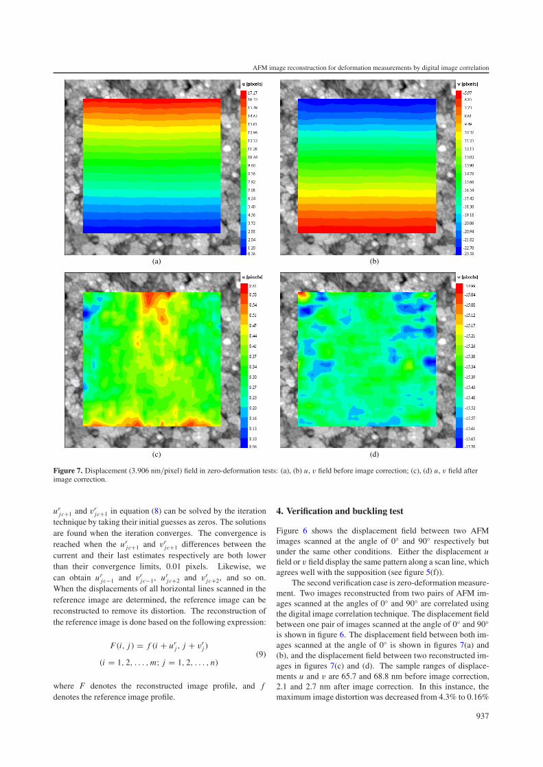
Figure 7. Displacement (3.906 nm/pixel) field in zero-deformation tests: (a), (b) u, v field before image correction; (c), (d) u, v field afterimage correction.

urjc+1 and vr

jc+1 in equation (8) can be solved by the iterationtechnique by taking their initial guesses as zeros. The solutionsare found when the iteration converges. The convergence isreached when the ur

jc+1 and vrjc+1 differences between the

current and their last estimates respectively are both lowerthan their convergence limits, 0.01 pixels. Likewise, wecan obtain ur

jc−1 and vrjc−1, ur

jc+2 and vrjc+2, and so on.

When the displacements of all horizontal lines scanned in thereference image are determined, the reference image can bereconstructed to remove its distortion. The reconstruction ofthe reference image is done based on the following expression:

F(i, j ) = f (i + urj , j + vr

j )

(i = 1, 2, . . . , m; j = 1, 2, . . . , n)(9)

where F denotes the reconstructed image profile, and fdenotes the reference image profile.

4. Verification and buckling test

Figure 6 shows the displacement field between two AFMimages scanned at the angle of 0◦ and 90◦ respectively butunder the same other conditions. Either the displacement ufield or v field display the same pattern along a scan line, whichagrees well with the supposition (see figure 5(f)).

The second verification case is zero-deformation measure-ment. Two images reconstructed from two pairs of AFM im-ages scanned at the angles of 0◦ and 90◦ are correlated usingthe digital image correlation technique. The displacement fieldbetween one pair of images scanned at the angle of 0◦ and 90◦is shown in figure 6. The displacement field between both im-ages scanned at the angle of 0◦ is shown in figures 7(a) and(b), and the displacement field between two reconstructed im-ages in figures 7(c) and (d). The sample ranges of displace-ments u and v are 65.7 and 68.8 nm before image correction,2.1 and 2.7 nm after image correction. In this instance, themaximum image distortion was decreased from 4.3% to 0.16%

937

Y Sun and J H L Pang

Table 1. Remaining strains in zero-deformation test.

Before correction After correction

Strains εx εy εx y εx εy εx y

Mean (ε) — — — 7.66 × 10−5 −1.24 × 10−4 −2.83 × 10−6

Min (ε) −3.78 × 10−3 3.01 × 10−2 −3.18 × 10−2 −4.92 × 10−3 −7.69 × 10−3 −4.25 × 10−3

Max (ε) 5.33 × 10−3 5.48 × 10−2 −1.16 × 10−2 5.50 × 10−3 6.78 × 10−3 3.97 × 10−3

σ (ε) — — — 1.48 × 10−3 1.80 × 10−3 1.24 × 10−3

Table 2. Strains measured by DIC and from FEA.

Strains εx εy εx y

Measured by DIC Mean (ε) 3.96 × 10−3 1.36 × 10−5 2.35 × 10−5

σ(ε) 6.96 × 10−4 3.91 × 10−4 3.58 × 10−4

FEA solution 3.88 × 10−3 6.59 × 10−8 2.20 × 10−9

(correlated image area is 1.6 µm × 1.6 µm). Therefore, thecorrection method to AFM images is effective to cancel out thedistortion shown in figures 7(a) and (b). In addition, a compar-ison of measured strains before and after image correction hasbeen listed in table 1. After image correction, the average re-maining strains, εx , εy and εx y , are 76.6, −124 and −2.83 µε,and their standard deviations 0.001 48, 0.001 80 and 0.001 24respectively, which shows the promise of accurate deformationmeasurements by digital image correlation.

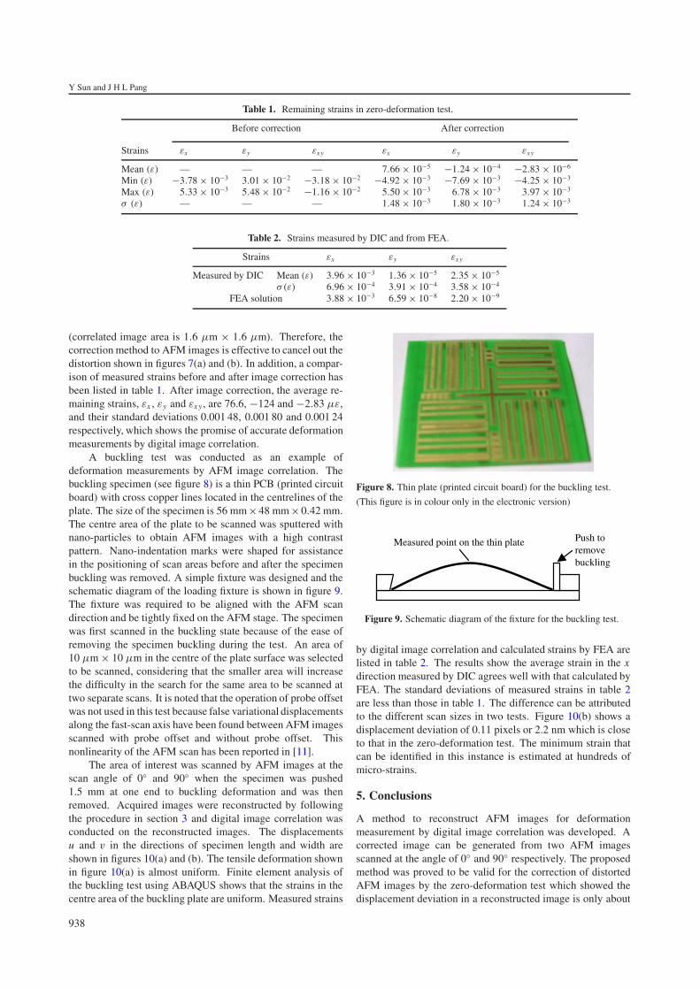
A buckling test was conducted as an example ofdeformation measurements by AFM image correlation. Thebuckling specimen (see figure 8) is a thin PCB (printed circuitboard) with cross copper lines located in the centrelines of theplate. The size of the specimen is 56 mm×48 mm ×0.42 mm.The centre area of the plate to be scanned was sputtered withnano-particles to obtain AFM images with a high contrastpattern. Nano-indentation marks were shaped for assistancein the positioning of scan areas before and after the specimenbuckling was removed. A simple fixture was designed and theschematic diagram of the loading fixture is shown in figure 9.The fixture was required to be aligned with the AFM scandirection and be tightly fixed on the AFM stage. The specimenwas first scanned in the buckling state because of the ease ofremoving the specimen buckling during the test. An area of10 µm × 10 µm in the centre of the plate surface was selectedto be scanned, considering that the smaller area will increasethe difficulty in the search for the same area to be scanned attwo separate scans. It is noted that the operation of probe offsetwas not used in this test because false variational displacementsalong the fast-scan axis have been found between AFM imagesscanned with probe offset and without probe offset. Thisnonlinearity of the AFM scan has been reported in [11].

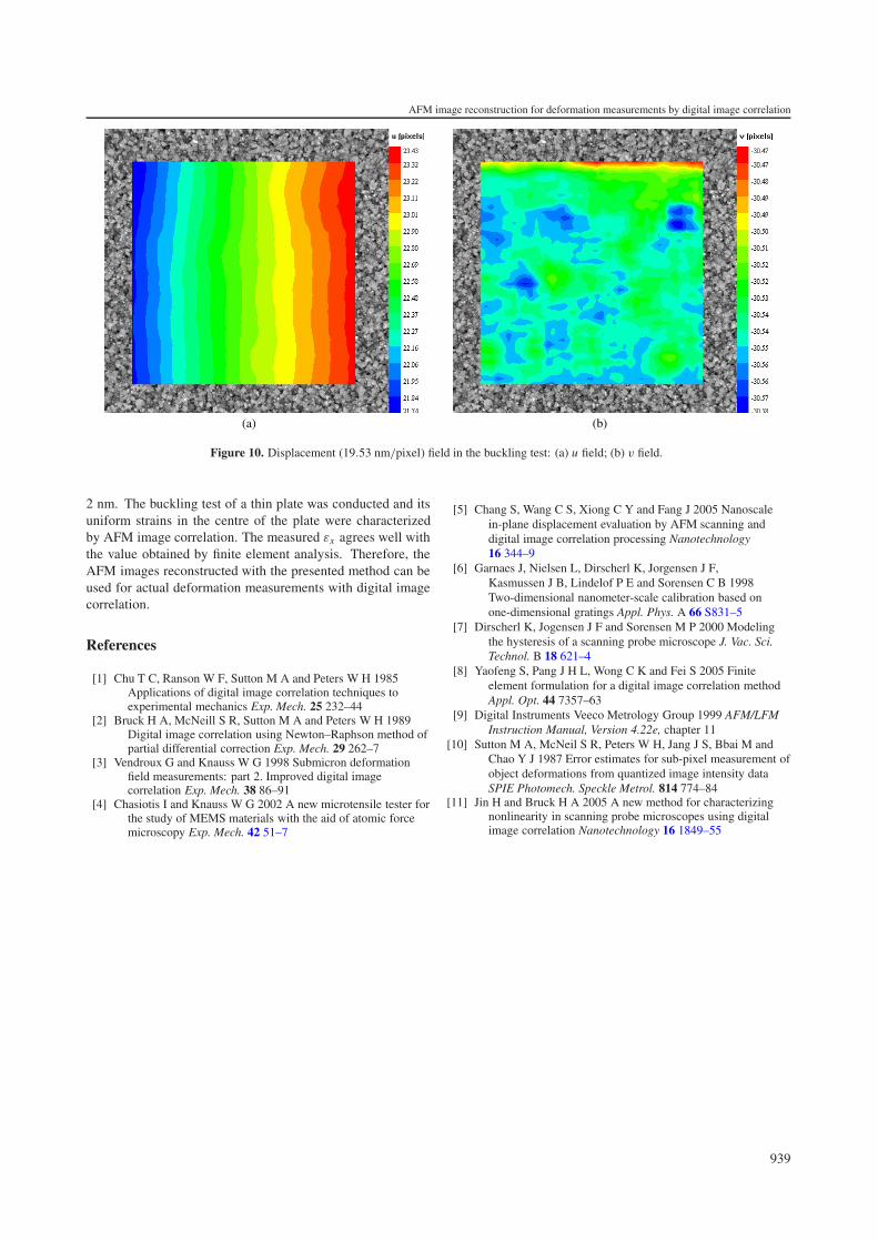
The area of interest was scanned by AFM images at thescan angle of 0◦ and 90◦ when the specimen was pushed1.5 mm at one end to buckling deformation and was thenremoved. Acquired images were reconstructed by followingthe procedure in section 3 and digital image correlation wasconducted on the reconstructed images. The displacementsu and v in the directions of specimen length and width areshown in figures 10(a) and (b). The tensile deformation shownin figure 10(a) is almost uniform. Finite element analysis ofthe buckling test using ABAQUS shows that the strains in thecentre area of the buckling plate are uniform. Measured strains

Figure 8. Thin plate (printed circuit board) for the buckling test.

(This figure is in colour only in the electronic version)

Measured point on the thin plate Push toremovebuckling

Figure 9. Schematic diagram of the fixture for the buckling test.

by digital image correlation and calculated strains by FEA arelisted in table 2. The results show the average strain in the xdirection measured by DIC agrees well with that calculated byFEA. The standard deviations of measured strains in table 2are less than those in table 1. The difference can be attributedto the different scan sizes in two tests. Figure 10(b) shows adisplacement deviation of 0.11 pixels or 2.2 nm which is closeto that in the zero-deformation test. The minimum strain thatcan be identified in this instance is estimated at hundreds ofmicro-strains.

5. Conclusions

A method to reconstruct AFM images for deformationmeasurement by digital image correlation was developed. Acorrected image can be generated from two AFM imagesscanned at the angle of 0◦ and 90◦ respectively. The proposedmethod was proved to be valid for the correction of distortedAFM images by the zero-deformation test which showed thedisplacement deviation in a reconstructed image is only about

938

AFM image reconstruction for deformation measurements by digital image correlation

(a) (b)

Figure 10. Displacement (19.53 nm/pixel) field in the buckling test: (a) u field; (b) v field.

2 nm. The buckling test of a thin plate was conducted and itsuniform strains in the centre of the plate were characterizedby AFM image correlation. The measured εx agrees well withthe value obtained by finite element analysis. Therefore, theAFM images reconstructed with the presented method can beused for actual deformation measurements with digital imagecorrelation.

References

[1] Chu T C, Ranson W F, Sutton M A and Peters W H 1985Applications of digital image correlation techniques toexperimental mechanics Exp. Mech. 25 232–44

[2] Bruck H A, McNeill S R, Sutton M A and Peters W H 1989Digital image correlation using Newton–Raphson method ofpartial differential correction Exp. Mech. 29 262–7

[3] Vendroux G and Knauss W G 1998 Submicron deformationfield measurements: part 2. Improved digital imagecorrelation Exp. Mech. 38 86–91

[4] Chasiotis I and Knauss W G 2002 A new microtensile tester forthe study of MEMS materials with the aid of atomic forcemicroscopy Exp. Mech. 42 51–7

[5] Chang S, Wang C S, Xiong C Y and Fang J 2005 Nanoscalein-plane displacement evaluation by AFM scanning anddigital image correlation processing Nanotechnology16 344–9

[6] Garnaes J, Nielsen L, Dirscherl K, Jorgensen J F,Kasmussen J B, Lindelof P E and Sorensen C B 1998Two-dimensional nanometer-scale calibration based onone-dimensional gratings Appl. Phys. A 66 S831–5

[7] Dirscherl K, Jogensen J F and Sorensen M P 2000 Modelingthe hysteresis of a scanning probe microscope J. Vac. Sci.Technol. B 18 621–4

[8] Yaofeng S, Pang J H L, Wong C K and Fei S 2005 Finiteelement formulation for a digital image correlation methodAppl. Opt. 44 7357–63

[9] Digital Instruments Veeco Metrology Group 1999 AFM/LFMInstruction Manual, Version 4.22e, chapter 11

[10] Sutton M A, McNeil S R, Peters W H, Jang J S, Bbai M andChao Y J 1987 Error estimates for sub-pixel measurement ofobject deformations from quantized image intensity dataSPIE Photomech. Speckle Metrol. 814 774–84

[11] Jin H and Bruck H A 2005 A new method for characterizingnonlinearity in scanning probe microscopes using digitalimage correlation Nanotechnology 16 1849–55

939