Embed Size (px)
Citation preview

The Journal of Economic History, Vol. 62, No. 2 (June 2002). © The Economic HistoryAssociation. All rights reserved. ISSN 0022-0507.
Kevin H. O’Rourke, Department of Economics and IIIS, Trinity College, Dublin 2, Ireland, andCEPR and NBER. E-mail: [email protected]. Jeffrey G. Williamson, Department of Economics,Harvard University, Cambridge, MA 02138, and NBER. E-mail: [email protected].
The authors acknowledge with pleasure the excellent research assistance of Ximena Clark, DavidFoster, and Raven Saks, plus help with the rent data from Greg Clark, Phil Hoffman, and Jan Luitenvan Zanden. An earlier version of this article was improved by comments from Arne Bigsten, JohnCoatsworth, Kirti Chaudhuri, Don Davis, Ron Findlay, Andre Gunder Frank, Elhanan Helpman, DougIrwin, Ron Jones, Lars Jonung, Paul Krugman, Peter Lindert, Pat Manning, Bob Mundell, Cormac ÓGráda, Gunnar Persson, Dick Sylla, participants at the Ohlin Conference (Stockholm, October 14–16,1999) and the festschrift conference in honor of Ronald Findlay (New York, April 20–21, 2001), andseminar participants at Copenhagen, Gotenborg, Harvard, LSE, and the Stockholm School of Econom-ics. In addition, we are grateful for the very useful and detailed comments of Jan de Vries and threereferees of this JOURNAL. Williamson also acknowledges generous research support from the NationalScience Foundation SBR-9505656 and SES-0001362. The usual disclaimer applies.
1 Krugman, “Growing World Trade,” p. 328; see also Feenstra, “Integration.”2 Baier and Bergstrand, “Growth.”
417
After Columbus: Explaining Europe’sOverseas Trade Boom, 1500–1800
KEVIN H. O’ROURKE AND JEFFREY G. WILLIAMSON
This study documents the boom in Europe’s imports from Asia and the Americasbetween 1500 and 1800 and explores its causes. There was no commodity-priceconvergence between continents, suggesting that declining trade barriers were not thecause of the boom. Thus, it must have been caused by some combination of Europeanimport demand and foreign export supply. The behavior of the relative price of for-eign importables in European cities should tell us which mattered most and when: weprovide the evidence and offer a model which is used to decompose the sources ofEurope’s overseas trade boom.
Why has world trade grown? This fundamental question has been posedrecently by notable international economists such as Paul Krugman.
In Krugman’s words: “Most journalistic discussion of the growth of worldtrade seems to view growing integration as driven by a technological im-perative—to believe that improvements in transportation and communica-tion technology constitute an irresistible force dissolving national bound-aries.”1 An alternative explanation might stress instead declining politicalbarriers to trade, which (like transport improvements) help link distant mar-kets together and erase commodity-price gaps between them. A third poten-tial explanation seems to have been even more powerful in practice, sinceit appears that fully two-thirds of the late-twentieth-century trade boom canbe explained by unusually fast income growth.2
This modern debate has a powerful historical resonance. For some time,scholars have written of a secular Euro-Asian and Euro-American tradeboom following the Voyages of Discovery by Christopher Columbus, Vasco

418 O’Rourke and Williamson
3 In one of his first forays into history, Ronald Findlay (“Trade”) used just such relative-priceevidence in an attempt to decompose the sources of trade growth during the Industrial Revolution.
da Gama and their followers. This article measures, we believe for the firsttime, the size and timing of that boom. Furthermore, and just as in the late-twentieth-century case discussed by Krugman, the most obvious explanationfor the post-Columbus trade boom would seem to be declining trade costsover the new sea routes. We shall argue that the evidence collected so far isinconsistent with this view, and then offer a model and the evidence neces-sary to decompose the sources of the trade boom into the demand and supplyfundamentals that seem to have mattered most.
The next section measures the trade boom as it was manifested by Europeanimports from, and exports to, both Asia and the Americas. The evidence thereshows that the share of trade in GDP has certainly increased over the 500 yearssince 1492. However, it also documents that some centuries underwent far big-ger trade booms than others. We then ask whether the boom can be explainedby declining trade barriers. If there was such a decline, then it should have lefta trail of shrinking commodity-price gaps between trading partners. There is nosuch evidence, suggesting that “discovery” and transport productivity improve-ments were offset by trading monopoly markups, government restrictions, wars,and pirates, all of which served in combination to choke off some of the trade.
If declining trade barriers do not explain Europe’s intercontinental tradeboom after Columbus, what does? The following section offers the leadingcontenders on the demand and supply sides. It also offers some importantnew evidence: it measures the relative price of many imports from Asia andthe Americas, quoted in European urban markets, over the five centuriesbetween 1350 and 1850. These relative prices are the smoking guns thatsuggest when European demand and overseas supply dominated and whethersupply from Asia and the Americas behaved differently.3 The section alsooffers estimates of the growth in Europe’s “surplus” income, presumably thecentral force driving European import demand. The next section develops anexplicit partial-equilibrium model and the actual decomposition of the tradeboom sources, century-by-century, from Columbus to the Crystal Palace. Wego on to speculate further on the sources of the trade boom, including thepossible role of a Chinese (and Korean and Japanese) retreat from worldmarkets from the mid-fifteenth century onwards. We finish with suggestionsfor future research, including a call for Asian and Latin American price histo-ries which would help sort out what was driving world trade before 1800.
EUROPE’S INTERCONTINENTAL TRADE BOOM AFTER COLUMBUS
Table 1 documents the Euro-Asian and Euro-American trade boom be-tween 1500 and 1800, which is the focus of this study, as well as the world

After Columbus 419
TABLE 1FIVE CENTURIES OF EUROPEAN INTERCONTINENTAL AND WORLD TRADE
GROWTH, 1500–1992
Trade Route/Type
GrowthPer Annum
(%) Denomination Abbreviated Source
1500–1549
Portugal to/from Asia 1.37 tonnage Prakesh, 32Southeast Asia spice exports 2.53 exports (1940US$) Bulbeck, 12–13Cloth exports from London 1.84 export volume Fisher, 96Shipping volume to/from Span Indies 3.94 toneladas Phillips, 43–44
Average 2.42
1550–1599
Portugal to/from Asia 0.94 tonnage Prakesh, 32Southeast Asia spice exports 2.31 exports (1940US$) Bulbeck, 12–13Cloth exports from London 0.10 export volume Fisher, 96Shipping volume to/from Span Indies 1.22 toneladas Phillips, 43–44Sugar exports from Span colonies –6.11 weight Phillips, 58–59Sugar exports from Port colonies 0.68 weight Phillips, 60–62Hide exports from Span colonies 1.73 number Phillips, 70–72
Average 0.12
1600–1649
Portugal to/from Asia –3.36 tonnage Prakesh, 32Southeast Asia spice exports 0.71 exports (1940US$) Bulbeck, 12–13Dutch East India to Asia 1.62 tonnage Prakesh, 104Dutch East India from Asia 2.17 tonnage Prakesh, 104Dutch East India imports from Asia 2.71 imports (florins) Prakesh, 115Dutch East India from Coromandel 2.76 exports (florins) Prakesh, 180Dutch East India from Gujarat 1.65 export (florins) Prakesh, 185English tobacco imports from Amer 0.12 imports (kilos) Steensgaard, 141English East India to Asia 2.99 exports (£) Prakesh, 106Shipping volume to/from Span Indies –1.70 toneladas Phillips, 43–44Sugar exports from Span colonies 0.15 weight Phillips, 58–59Sugar exports from Port colonies 0.92 weight Phillips, 60–62Hide exports from Span colonies –0.96 number Phillips, 70–72
Average 0.75
1650–1699
Portugal to/from Asia 0.25 tonnage Prakesh, 32Southeast Asia spice exports –0.33 exports (1940US$) Bulbeck, 12–13Dutch East India to Asia 0.48 tonnage Prakesh, 104Dutch East India from Asia 0.63 tonnage Prakesh, 104Dutch East India imports from Asia 0.12 imports (florins) Prakesh, 115Dutch East India from Coromandel 1.65 exports (florins) Prakesh, 180Dutch East India from Gujarat 0.17 exports (florins) Prakesh, 185Dutch East India from Bengal 3.07 exports (florins) Prakesh, 196Dutch from Asia 0.33 exports (florins) Prakesh, 203Dutch copper imports from Japan 0.23 imports (Dutch lbs.) Glamann, 52–53English East India to Asia 2.79 exports (£) Prakesh, 106English East India from Asia –1.23 imports (£) Chaudhuri, 508–10English East India textiles from Asia 0 imports (£) Chaudhuri, 547–48
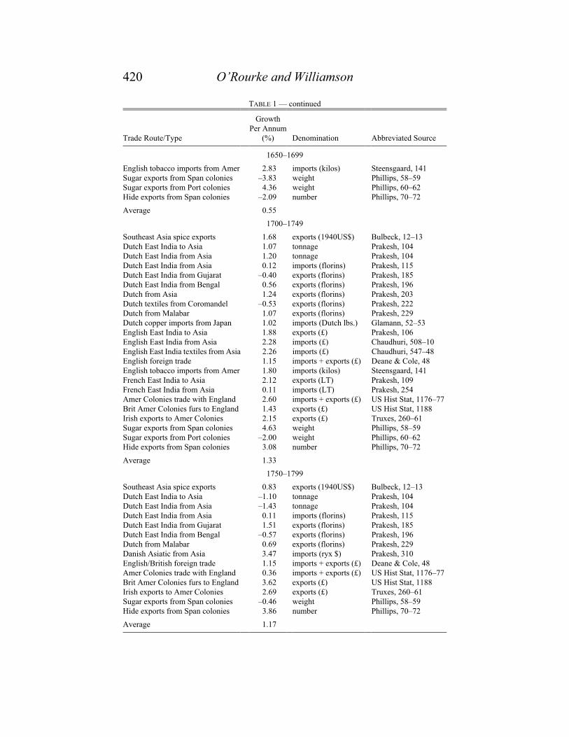
420 O’Rourke and Williamson
TABLE 1 — continued
Trade Route/Type
GrowthPer Annum
(%) Denomination Abbreviated Source
1650–1699
English tobacco imports from Amer 2.83 imports (kilos) Steensgaard, 141Sugar exports from Span colonies –3.83 weight Phillips, 58–59Sugar exports from Port colonies 4.36 weight Phillips, 60–62Hide exports from Span colonies –2.09 number Phillips, 70–72
Average 0.55
1700–1749
Southeast Asia spice exports 1.68 exports (1940US$) Bulbeck, 12–13Dutch East India to Asia 1.07 tonnage Prakesh, 104Dutch East India from Asia 1.20 tonnage Prakesh, 104Dutch East India from Asia 0.12 imports (florins) Prakesh, 115Dutch East India from Gujarat –0.40 exports (florins) Prakesh, 185Dutch East India from Bengal 0.56 exports (florins) Prakesh, 196Dutch from Asia 1.24 exports (florins) Prakesh, 203Dutch textiles from Coromandel –0.53 exports (florins) Prakesh, 222Dutch from Malabar 1.07 exports (florins) Prakesh, 229Dutch copper imports from Japan 1.02 imports (Dutch lbs.) Glamann, 52–53English East India to Asia 1.88 exports (£) Prakesh, 106English East India from Asia 2.28 imports (£) Chaudhuri, 508–10English East India textiles from Asia 2.26 imports (£) Chaudhuri, 547–48English foreign trade 1.15 imports + exports (£) Deane & Cole, 48English tobacco imports from Amer 1.80 imports (kilos) Steensgaard, 141French East India to Asia 2.12 exports (LT) Prakesh, 109French East India from Asia 0.11 imports (LT) Prakesh, 254Amer Colonies trade with England 2.60 imports + exports (£) US Hist Stat, 1176–77Brit Amer Colonies furs to England 1.43 exports (£) US Hist Stat, 1188Irish exports to Amer Colonies 2.15 exports (£) Truxes, 260–61Sugar exports from Span colonies 4.63 weight Phillips, 58–59Sugar exports from Port colonies –2.00 weight Phillips, 60–62Hide exports from Span colonies 3.08 number Phillips, 70–72
Average 1.33
1750–1799
Southeast Asia spice exports 0.83 exports (1940US$) Bulbeck, 12–13Dutch East India to Asia –1.10 tonnage Prakesh, 104Dutch East India from Asia –1.43 tonnage Prakesh, 104Dutch East India from Asia 0.11 imports (florins) Prakesh, 115Dutch East India from Gujarat 1.51 exports (florins) Prakesh, 185Dutch East India from Bengal –0.57 exports (florins) Prakesh, 196Dutch from Malabar 0.69 exports (florins) Prakesh, 229Danish Asiatic from Asia 3.47 imports (ryx $) Prakesh, 310English/British foreign trade 1.15 imports + exports (£) Deane & Cole, 48Amer Colonies trade with England 0.36 imports + exports (£) US Hist Stat, 1176–77Brit Amer Colonies furs to England 3.62 exports (£) US Hist Stat, 1188Irish exports to Amer Colonies 2.69 exports (£) Truxes, 260–61Sugar exports from Span colonies –0.46 weight Phillips, 58–59Hide exports from Span colonies 3.86 number Phillips, 70–72
Average 1.17

After Columbus 421
4 The focus is on commodities other than silver and gold, since these precious metals played amonetary role as well as a more standard commodity role, and different factors thus explain their largeand growing importance in international trade during the period. We are interested solely in the growthof nonmonetary commodity trade, and as such the large literature on the impact of intercontinentalsilver flows on aggregate price levels, while fascinating and important, is not relevant here.
5 Maddison, Monitoring.6 We have made no judgments about the quality of the various data reported in Table 1. Thus, sugar
exports from the Americas 1550–1599 appear twice, once from the Spanish colonies and once fromthe Portuguese colonies. We have explored all kinds of recombinations and exclusions with the datain Table 1. Consider one of these. Table 1 computes an unweighted average of the growth rates under-lying all series in each half-century after 1500, and then cumulates these half-century growth rates to
TABLE 1 — continued
Trade Route/Type
GrowthPer Annum
(%) Denomination Abbreviated Source
1820–1849
World constant-price exports 4.18 exports (1990US$) Maddison, 239
1850–1899
World constant-price exports 3.64 exports (1990US$) Maddison, 239
1900–1950
World constant-price exports 2.00 exports (1990US$) Maddison, 239
1950–1992
World constant-price exports 5.65 exports (1990US$) Maddison, 239
1500–1599 1.26 (volume only: 1.26)1600–1699 0.66 (volume only: 0.11)1700–1799 1.26 (volume only: 0.90)1500–1799 1.06 (volume only: 0.76)1820–1899 3.851900–1992 3.651820–1992 3.70
Notes: Some of the within-half-century series were shorter than 50 years, but we used them anywayas long as the route/type time series in question covered more than 25 years. We often had tointerpolate between benchmark dates, but the vast majority of the half-century average per annum ratesreported above are calculated from an estimated equation where route/type figures have been regressedon time and time squared for the half-century in question. The half century averages are unweighted.Sources: Bulbeck et al., Southeast Asian Exports; Chaudhuri, Trading World; Deane and Cole, British
Economic Growth; Fisher, “Commercial Trends”; Glamann, “Dutch East India Company’s Trade”;Maddison, Monitoring; Phillips, “Growth”; Prakesh, New Cambridge History; Steensgaard, “Growth”;Truxes, “Irish–American Trade”; and U.S. Department of Commerce, Historical Statistics.
trade boom which occurred thereafter.4 The evidence summarized theretakes many forms, and it is never quite what we would like: sometimes tradewas reported in values, sometimes in volumes; sometimes for one product,sometimes for another; sometimes carried by one country, sometimes an-other; and it is never—at least until 1820—a constant-price world tradeindex.5 Still, the regional, product, and country coverage is enormous.6 Inany case, it’s all that the archives have yielded thus far.
422 O’Rourke and Williamson
yield 1.06 percent per annum between 1500 and 1800. Alternatively, one can include in the calculationonly those series describing European imports from Asia and the Americas, since in the presence ofbullion flows Europe’s export growth need not have equaled its import growth, and since we will laterbe appealing to European import demand in our attempt to account for these trade flows. However, thetwo calculations yield much the same result: 1.06 versus 0.97 percent per annum. With only oneexception, the main findings documenting trade growth from 1500 to 1800 reported in the text changevery little with each alternative treatment of the data. The exception is reported in footnote 8.
7 Maddison, Monitoring, p. 227.8 We also calculated trade growth rates excluding all nominal series on the premise that it is the
volume of trade that must be explained, not the value. If prices were falling, the 1.1 percent growth ratewould understate trade volume growth, while the reverse would be true if prices were rising. Excludingall the nominal series in Table 1 lowers trade growth from 0.66 to 0.11 percent per annum in theseventeenth century, a big decline. The problem with this procedure, of course, is that it rejects datafrom routes and carriers which are then poorly represented. For example, in the period 1650–1699,when the impact of the procedure is biggest, it rejects nine of the seventeen observations, all of whichreport on Dutch and English East Indian trade! Overall, excluding the nominal series lowers growthover the three centuries from 1.06 to 0.76 percent per annum. These differences are big enough tosuggest that we use both—thus establishing upper and lower bounds—when we decompose the sourcesof the trade boom. It will not influence our key findings.
9 The 1760 share falls before recovering an all-time high in 1801: see Crafts, British Economic
Growth, table 6.6, p. 131.
The panel at the bottom of Table 1 reports two notable facts. First, thegrowth of world trade was pretty much the same in the nineteenth and twen-tieth centuries, roughly 3.7 or 3.8 percent per annum. This is a surprisingfact, given that world GDP growth doubled from 1.5 to 3 percent per annumbetween 1820–1913 and 1913–1992.7 Since the growth of world trade wasalmost identical in the two centuries, it follows that trade shares rose muchfaster in the nineteenth than in the twentieth century. So far, it looks asthough the nineteenth century is the canonical globalization epoch par excel-
lence. Second, Europe’s intercontinental trade growth prior to 1800 wasmuch slower, about 1.1 percent per annum. Of course, everything else grewmore slowly in this preindustrial period too, so 1.1 percent may still be fastenough to ensure that Europe’s trade shares were on the increase in the wakeof da Gama and Columbus.8 They were certainly on the increase ineighteenth-century Britain, where the export to GNP ratio rose from 8.4percent in 1700, to 14.6 percent in 1760, and to 15.7 percent in 1801.9
Can this 1.1 percent per annum growth rate in Europe’s intercontinentaltrade be explained by declining trade costs? This is the central questionmotivating this essay.
WAS THE TRADE BOOM DRIVEN BY MARKET INTEGRATION?
The most obvious explanation for Europe’s intercontinental trade boomis that it was caused by “discovery,” declining transport costs, and/or somefall in man-made barriers to trade. We shall call this view the “market inte-gration” hypothesis; it implies that discovery and declining transport costsconverted potential trading partners into actual trading partners by lowering

After Columbus 423
10 Findlay, “Emergence,” pp. 53–54.11 Prakesh, New Cambridge History, table 4.1, p. 115.12 Ibid., table 2.2, p. 35.13 Ibid., table 2.3, p. 36.14 Ibid., table 4.2, p. 120.15 Small impact does not, of course, mean no impact at all. To the extent that imported silk cloth
displaced some domestic woolen cloth consumption in Europe, the prices of woolen cloth would havefallen. However, only the rich bought imported silk cloth, so the impact on domestic woolens produc-tion and prices would have been small. Similarly for spices and other imported exotics. The impact oftea imports on beer consumption and production, late in our period, may well have been a differentmatter.
the cost of doing business between them. If this hypothesis is correct, thenwe should be able to document commodity-price convergence betweenEurope, Asia, and the Americas over the three centuries. After all, a declinein the costs of doing business between two markets must be reflected inshrinking price gaps between them. If we cannot document Euro-Asian orEuro-American commodity-price convergence, then the market integrationhypothesis must be rejected and we will have to search for other explana-tions of Europe’s intercontinental trade boom.
Where, then, should we look for evidence of intercontinental marketintegration? Initially, only goods with very high value-to-bulk ratios—suchas silk, exotic spices, and precious metals—were shipped. Indeed, Europeanlong distance trade before the eighteenth century was strictly limited to whatinternational economists call noncompeting goods: Europe imported spices,silk, sugar, and gold, items which were not produced there at all, or at leastwere in very scarce supply; Asia imported silver, linens, and woolens, whichwere not found there at all (with the important exception of Japanese silverbefore 1668). Dutch exports of precious metals to Asia accounted for be-tween half and two-thirds of the value of Asian products imported into Eu-rope by the Dutch East India Company (Vereenigde Oostindische Com-pagnie, or simply VOC),10 whereas VOC imports into Europe were domi-nated by spices, tea, coffee, drugs, perfumes, dyestuffs, sugar, and saltpetre.Indeed these were 84 percent of the VOC import total in 1619/1621, 73percent in 1698/1700, and still a hefty 64 percent as late as 1778/1780.11
Imports into Lisbon from Asia were almost entirely spices in 1518.12 Tex-tiles came to take a larger share of that total, but spices were still 88 percentof Asian imports into Lisbon by 1610.13 Even the English East India Com-pany, famous for their gamble of focusing on the Indian textile trade, hadimports heavily weighted by spices and other luxuries: their share was 43.4percent in 1668/1670 and 46.5 percent in 1758/1760.14 These noncompetinggoods were very expensive luxuries in importing markets, and thus couldbear the very high cost of transportation from their (cheap) sources. Bydefinition, their presence or absence in Europe had only a small impact ondomestic production since they were noncompeting.15

424 O’Rourke and Williamson
16 O’Rourke and Williamson, “Heckscher–Ohlin Model” and “When Did Globalization?”17 Steensgaard, “Freight Costs,” p. 148.18 Ibid., table 1, pp. 152 and 154.19 We say “most” but do not assert “all.” Presumably, the VOC saved on costs by switching to a
permanent Asian fleet. In Steengaard’s words, “The extra expense involved in setting up this perma-nent Asian trading fleet must have been slight compared with the saving achieved by employing thebig return ships solely for the purpose for which they were intended” (ibid., p. 156).
20 Davis, Rise, pp. 262–64; and Krishna, Commercial Relations, pp. 321–23.21 As paraphrased by Menard, “Transport Costs,” p. 250.22 Davis, Rise, p. 263; and Chaudhuri, Trading World, tables C.20 and C.22.23 Reid, Southeast Asia, pp. 288–89.
So what is the evidence of price convergence for those commoditieswhich were traded during the Age of Commerce between Europe and Asia,and between Europe and the Americas? Elsewhere we have reviewed thisevidence in detail, so the rest of this section only offers a brief survey offreight rates and commodity-price convergence since 1492.16
At the beginning of the seventeenth century, freight costs on the round-trip voyage from Europe to the East Indies were £30–32 per ton, whethercarried in a Dutch or an English vessel.17 A half-century later, freight costson English chartered ships had fallen to £16–23, or by 23–50 percent, animpressive decline on the face of it. However, it turns out that the source ofthe decline was a fall in the turnaround time in Southeast Asia.18 Prior to1640, Dutch and English East India Company ships were required to spendtime putting down local revolts in Asian waters, building forts, negotiatingagreements, showing the flag, and fending off European competitors. After1640, chartered ships did not perform these functions, but rather a perma-nent fleet of smaller East India Company ships did. Freight costs do notinclude the cost of the permanent fleet, borne by the East India Companiesas before; when these costs are added back in, our guess is that most of thedecline in transport costs over the half-century would evaporate.19 RalphDavis and Bal Krishna have extended the freight-cost evidence from the1650s to the 1730s.20 They find that freight costs “were higher in the 1720sand 1730s than they had been in the 1660s and 1670s and they took anotherstep upward in the 1760s, when they return to the levels prevailing in theearly seventeenth century.”21 Freight rates for “fine” textiles shipped toEngland from the Malabar Coast and Bay of Bengal or from Bombay andSurat show no sign of decline in the eighteenth century when deflated by theaverage prices paid for Bengali and Bombay textiles, respectively.22 As faras we can tell, there is no evidence of any transport revolution along Euro-Asian trade routes during the Age of Commerce.
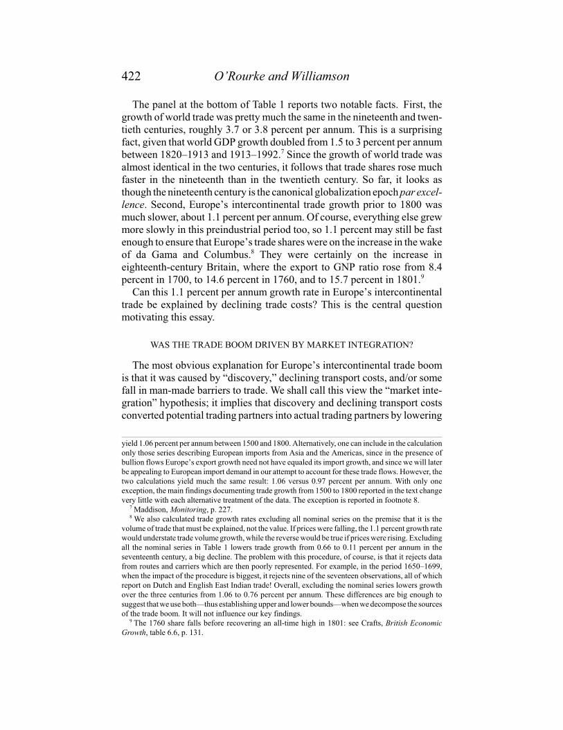
More importantly, what about commodity-price convergence? We havethe requisite price data for spices and coffee, items which combined were 68percent of Dutch homeward cargoes in the mid-seventeenth century.23
Figure 1 plots markups for cloves, pepper and coffee, where markups are

After Columbus 425
24 Bulbeck et al., Southeast Asian Exports.
0
5
10
15
20
25
1580s 1610s 1640s 1670s 1700s 1730s 1760s 1790s 1820s 1850s 1880s 1910s
Decade
Sal
es p
rice
/ P
urch
ase
pric
eCloves
Black pepper
Coffee
FIGURE 1SPICE AND COFFEE MARK-UPS, 1580–1939
(Amsterdam vs. Southeast Asia)
Sources: See the text.
defined as the ratio of European to Asian price.24 There is plenty of evidenceof price convergence for cloves from the 1590s to the 1640s, but it wasshort-lived: the spread soared to a 350-year high in the 1660s, maintainingthat high level during the VOC monopoly and up to the 1770s. The clove-price spread fell steeply at the end of the French Wars, and by the 1820s wasone-fourteenth of the 1730s level. This low spread was maintained acrossthe nineteenth century. There was a slight upward trend in the mark-up onpepper between the 1620s and the 1770s, after which it soared to a 250-yearhigh in the 1790s. By the 1820s, the pepper-price spread of the early seven-teenth century was restored, and price convergence continued up to the1880s, when the series ends. While there is some modest evidence of priceconvergence for coffee during the half-century between the 1730s and the1780s, everything gained was lost and more during the French Wars. At thewar’s end, price convergence resumed, so that the coffee price spread in the1850s was one-sixth of what it had been in the 1750s, and in the 1930s itwas one-thirteenth of what it had been in the 1730s. Thus, for the period1640–1800 there is precious little evidence of commodity-price convergencefor these “exotic” goods so central to Dutch trade. Was English trade in Asia

426 O’Rourke and Williamson
25 O’Rourke and Williamson, “When Did Globalization?” figures 8A–F.26 A reading of Douglas Irwin (“Mercantilism,” especially p. 1297) suggests that pretty much all
intercontinental trade at this time was by state-chartered monopolies. Like most monopolies, they raisedprices paid by consumers (in Europe), lowered prices paid by suppliers (in Asia), restricted output, andlimited trade. This is hardly the stuff that globalization is made of! However, an insightful referee haspointed out that the investments in exploration and discovery probably would never have been madewithout the ability of Columbus, da Gama, and their followers to internalize the returns to investmentsmade in the Voyages of Discovery. Economists have been debating the net balance between certainshort-term losses from monopoly and their uncertain long-term gains ever since Adam Smith. The issueis noted here but not resolved.
27 All import-price data come from Chaudhuri (Trading World, table C.24), which also provides dataon sales prices and mark-ups from 1664 to 1704. From 1710 to 1759, the sales prices used are thosegiven in Chaudhuri’s table A.13 (p. 302); like the earlier data in table C.24, these are average prices,but since they are listed in a separate table, we cannot be sure that they are strictly comparable withthose earlier figures.
any different than Dutch trade? Apparently not, at least based on the Anglo-Indian trade in pepper, tea, silk, coffee, and indigo.25
Of course, the price spread on pepper, cloves, coffee, tea, and other non-competing goods was not driven solely, or even mainly, by the costs ofshipping, but rather by monopoly,26 international conflict, piracy, and gov-ernment restrictions. Any one of these forces can raise or lower the barriersto trade, and historians have done excellent work on each for the varioustrade routes connecting Europe with Asia and the Americas. While thesearch for such forces is certainly valuable, this study is indifferent about thesources of net changes in trade barriers and in price gaps between markets.Ceteris paribus, anything that lowers price gaps between markets encour-ages trade, but there is no evidence of a secular erosion in Euro-Asian orEuro-American commodity-price gaps before the 1820s. The ceteris paribus
qualification is, of course, important since, as we shall see, something elsemust have accounted for Europe’s intercontinental trade boom if it was notdeclining trade barriers.
Is there any reason to expect the behavior of the price spread on compet-
ing goods between Europe and Asia to have differed from that of the non-
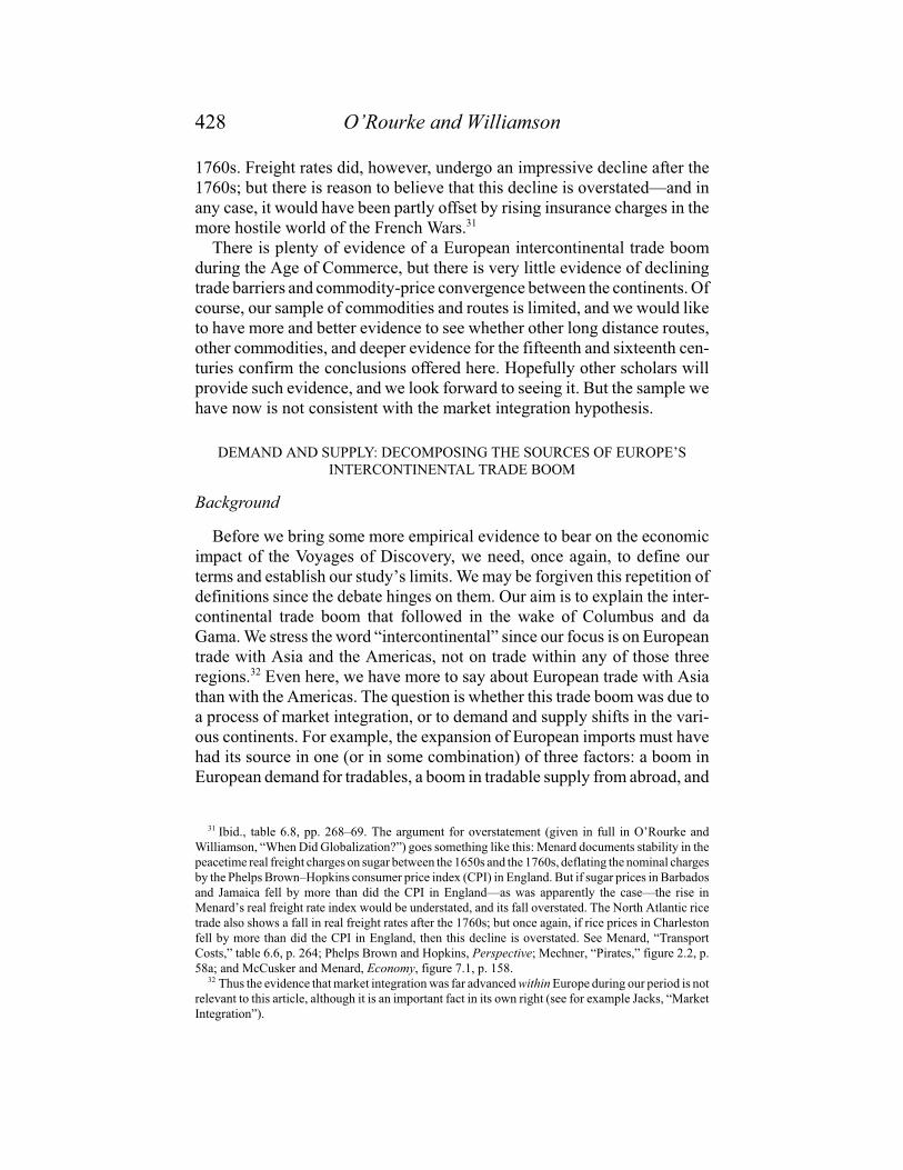
competing “exotics” we have just examined? We think it unlikely, especiallyif we cannot find any such divergence in the important English East Indiancloth trade. Figure 2 plots the East India Company’s “mark-up” (defined asfor Figure 1) on Asian textiles sold in Europe. Again, there is no sign of asecular decline over the century between 1664 and 1759.27 This textile tradewas extremely large, and it was on the rise. And yet the evidence on freightrates and mark-ups suggests that growing trade volumes in the late seven-teenth century were almost certainly driven by the outward expansion ofEuropean import demand or Asian export supply rather than by marketintegration per se. If it was market integration at work, we should see evi-dence of commodity price convergence and erosion in intercontinental pricegaps. Yet, we do not.

After Columbus 427
28 Menard, “Transport Costs.”29 Ibid., p. 255.30 Ibid., table 6.6, p. 264.
0
1
2
3
4
5
6
7
8
9
1660 1670 1680 1690 1700 1710 1720 1730 1740 1750
Sal
es p
rice
/ P
urch
ase
pric
e
FIGURE 2ASIAN TEXTILE MARK-UPS, 1664–1759
Sources: See the text.
The evolution of transport costs in the North Atlantic prior to the earlynineteenth century is summarized by Russell Menard.28 True, Menard’sinterest is in transport revolutions, and his evidence is thus limited to freightrates rather than commodity-price gaps, but his freight-cost indices offer nounambiguous support for declining barriers to trade and the market-integra-tion hypothesis. The best case for a pre-nineteenth-century transport revolu-tion in the North Atlantic lies with the tobacco trade. Between 1618 and1775, freight charges on tobacco shipments from the Chesapeake to Londonfell substantially: adjusted by the Phelps Brown–Hopkins consumer priceindex, real freight rates fell by 1.6 percent per annum over the entire colonialperiod.29 The worst case for a North American pre-nineteenth-century trans-port revolution lies with the sugar trade of Barbados and Jamaica, as well aswith the rice trade of Charleston, both with England. Menard documentsstability in the peacetime real freight charges on sugar between the 1650sand the 1760s, which tends to belie the market-integration hypothesis.30 Therice trade also shows no fall in real freight rates between the 1690s and the
428 O’Rourke and Williamson
31 Ibid., table 6.8, pp. 268–69. The argument for overstatement (given in full in O’Rourke andWilliamson, “When Did Globalization?”) goes something like this: Menard documents stability in thepeacetime real freight charges on sugar between the 1650s and the 1760s, deflating the nominal chargesby the Phelps Brown–Hopkins consumer price index (CPI) in England. But if sugar prices in Barbadosand Jamaica fell by more than did the CPI in England—as was apparently the case—the rise inMenard’s real freight rate index would be understated, and its fall overstated. The North Atlantic ricetrade also shows a fall in real freight rates after the 1760s; but once again, if rice prices in Charlestonfell by more than did the CPI in England, then this decline is overstated. See Menard, “TransportCosts,” table 6.6, p. 264; Phelps Brown and Hopkins, Perspective; Mechner, “Pirates,” figure 2.2, p.58a; and McCusker and Menard, Economy, figure 7.1, p. 158.
32 Thus the evidence that market integration was far advanced within Europe during our period is notrelevant to this article, although it is an important fact in its own right (see for example Jacks, “MarketIntegration”).
1760s. Freight rates did, however, undergo an impressive decline after the1760s; but there is reason to believe that this decline is overstated—and inany case, it would have been partly offset by rising insurance charges in themore hostile world of the French Wars.31
There is plenty of evidence of a European intercontinental trade boomduring the Age of Commerce, but there is very little evidence of decliningtrade barriers and commodity-price convergence between the continents. Ofcourse, our sample of commodities and routes is limited, and we would liketo have more and better evidence to see whether other long distance routes,other commodities, and deeper evidence for the fifteenth and sixteenth cen-turies confirm the conclusions offered here. Hopefully other scholars willprovide such evidence, and we look forward to seeing it. But the sample wehave now is not consistent with the market integration hypothesis.
DEMAND AND SUPPLY: DECOMPOSING THE SOURCES OF EUROPE’SINTERCONTINENTAL TRADE BOOM
Background
Before we bring some more empirical evidence to bear on the economicimpact of the Voyages of Discovery, we need, once again, to define ourterms and establish our study’s limits. We may be forgiven this repetition ofdefinitions since the debate hinges on them. Our aim is to explain the inter-continental trade boom that followed in the wake of Columbus and daGama. We stress the word “intercontinental” since our focus is on Europeantrade with Asia and the Americas, not on trade within any of those threeregions.32 Even here, we have more to say about European trade with Asiathan with the Americas. The question is whether this trade boom was due toa process of market integration, or to demand and supply shifts in the vari-ous continents. For example, the expansion of European imports must havehad its source in one (or in some combination) of three factors: a boom inEuropean demand for tradables, a boom in tradable supply from abroad, and
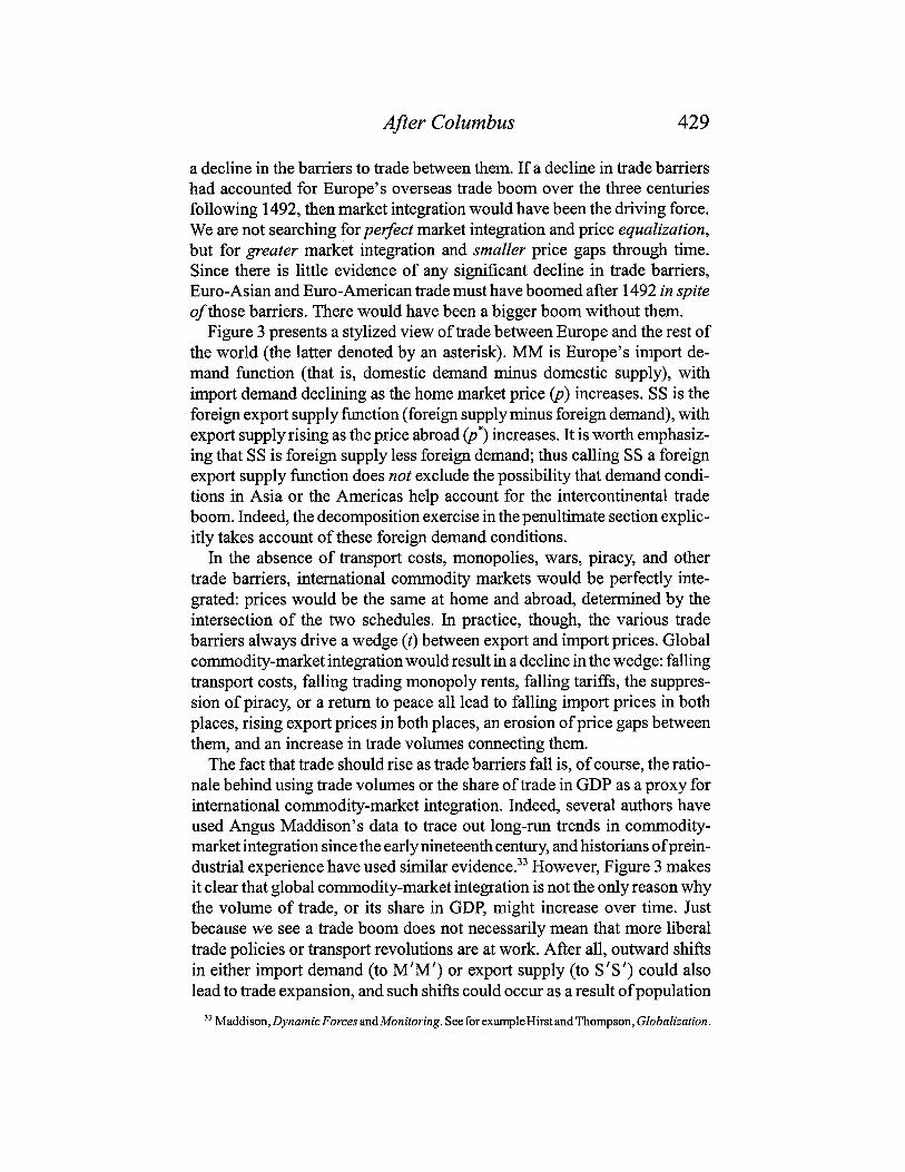

430 O’Rourke and Williamson
FIGURE 3
EXPLAINING EUROPE’S TRADE BOOM
Sources: See the text.
growth, the settlement of previously unexploited frontiers, capital accumula-
tion, technological change, a shift in income distribution favoring those who
import “exotic” luxuries, and a variety of other factors. Alternatively, global
commodity market integration could coincide with falling trade volumes, if
MM or SS were shifting inwards over time. Thus, Figure 3 argues that the
only irrefutable evidence of global commodity-market integration is a de-
cline in the international dispersion of commodity prices, or what we call
commodity-price convergence—i.e., precisely the event that we have failed
to discover.
We represent the post-1492 trade boom documented above as a rise from
T0 to T1, T2, or T3. If t remained constant (no net decline in trade barriers
and no move toward more global commodity market integration), then
outward shifts in either MM or SS, but not both, would generate a trade
boom to T1 (where the price gap, t, remains the same, although prices
change in both markets). An outward shift in both MM and SS would gen-
erate a bigger trade boom to T2. If at the same time t evaporated (com-
After Columbus 431
34 But see Hoffman et al., “Prices.”35 Hamilton, American Treasure, Money, and War; Posthumus, Inquiry; and Beveridge, Prices.36 These scholars also took great care with weights, measures, and quality. These commodities are
as close to being homogenous over these centuries as the most demanding historian would wish.37 Indeed, Appendix Table 1 shows that all we have for 1450–1500 is Posthumus on pepper and
ginger, and, even though ginger dominates, the two prices move in opposite directions! If pepper is
what was really motivating da Gama, then an account that emphasizes rising relative prices prompting
greater investment in exploration becomes more plausible. Ginger tells the opposite story, and Post-
humus cannot offer any other exotic noncompeting import prices to resolve the conflict. Thankfully,
the data grow much thicker after 1550.
plete global commodity market integration), we would observe an even
bigger trade boom to T3. Figure 3 is translated into an explicit “sources-of-
trade” equation and estimated in the penultimate section of the paper, where
the observed intercontinental trade boom is actually decomposed into the
component parts associated with shifts in European import demand and
overseas export supply.
Relative Price Trends
Figure 3 makes it clear that the behavior of the relative prices of spices, silk,
tea, sugar, and the many other “exotic” commodities imported into Europe
from overseas should tell us whether it was mainly foreign supply or mainly
domestic demand which accounted for Europe’s intercontinental trade boom
from 1500 to 1800. Appendix 1 reports in detail how we have calculated trends
in the prices of these European luxury imports relative to a local necessity that
did not travel between continents in those times, grain (wheat, oats, or barley,
depending on the source used). The evidence is very rich, and the sources well
known, which makes it all the more surprising that, as far as we know, they
have never been used for this purpose.34 Three famous scholars from a previ-
ous generation have left behind an amazing database describing prices for the
three main European participants in the overseas trade: Earl Hamilton on
Spain; Nicolaas Posthumus on the Netherlands; and William Beveridge on
England.35 These scholars documented (in most cases, annually) the prices of
spices, sugar, incense, indigo, tobacco, opium, coffee, tea, and other noncom-
peting importables from Asia and the Americas, as they prevailed in major
European cities such as Amsterdam, London, and Seville.36 We have used
these data to calculate trends in the relative price of noncompeting importables
in every half-century between 1350 and 1850. The findings are summarized in
Table 2, which reports Asian and American imports separately, as well as the
total.
The following seven facts emerge from Table 2. First, it was not some
spectacular boom in the relative price of all imported “exotic” prod-
ucts—bloating trading profits to even higher levels—that sent Columbus and
da Gama off to seek them. Granted, the evidence is thin—and, importantly,
relative pepper prices did rise in the second half of the fifteenth century37—

432 O’Rourke and Williamson
TABLE 2
CHANGES IN THE AVERAGE RELATIVE PRICE OF EUROPE’S NONCOMPETING
IMPORTABLES, 1350–1850
(percent per annum)
Asia America Total
1350–1400 1.16 n.a. 1.16
1400–1450 –0.58 n.a. –0.58
1450–1500 –0.11 n.a. –0.11
1400–1500 –0.35 n.a. –0.35
1500–1550 –0.72 0.44 –0.58
1550–1600 –1.38 0.53 –1.22
1500–1600 –1.05 0.48 –0.90
1600–1650 0.39 –0.41 0.14
1650–1700 0.78 –0.19 0.41
1600–1700 0.58 –0.30 0.28
1700–1750 –0.05 0.09 0.01
1750–1800 –0.49 –0.14 –0.34
1700–1800 –0.27 –0.02 –0.17
1500–1800 –0.25 0.05 –0.27
1800–1850 –1.38 –0.98 –1.15
Note: This summary table uses all the price data reported in Appendix Table 1. To do otherwise would
require judgments on the relative quality of the data that we do not possess. Thus, Asian pepper prices
in European markets are quoted for 1550–1600 four times, as are American sugar prices 1600–1650.
Source: Appendix Table 1.
but what we do have says that in general relative prices fell across the fif-
teenth century, and particularly in the first half of that century. Second, these
relative prices fell even faster in the sixteenth century, just as one would
expect if supply booms in Asia and the Americas were doing the work.
Indeed, the sixteenth-century collapse in those relative prices was bigger by
far than in any other period save 1800–1850. However, we believe that the
forces underlying relative price changes in these two centuries were com-
pletely different. It was not global market integration and commodity-price
convergence that accounted for the dramatic fall in relative prices during the
sixteenth century, but rather booming supply overseas. In contrast, declining
transport costs mattered a great deal in the early nineteenth century, espe-
cially since income growth in Europe was far faster then than at any other
time between 1500 and 1850, which would otherwise have raised the price
of importables. Third, the secular decline in relative prices stopped around
1600—actually rising across the seventeenth century—suggesting that a
boom in European demand or a collapse in Asian supply was dominant in
the seventeenth century. Fourth, the relative price of noncompeting imports
was more stable across the eighteenth century, suggesting that European
demand and foreign supply changes were more closely offsetting. However,
After Columbus 433
38 O’Rourke and Williamson, “Heckscher–Ohlin Model” and “When Did Globalization?”39 The American figures for the sixteenth century depend entirely on just one sugar-price series, so
we must be cautious about this finding for that century. However, the seventeenth century is much
more richly documented for the Americas, and the price observations are certainly not limited to sugar.
See Appendix Table 1.40 One reader has suggested that sugar from the Americas was an exception to this general rule, but
the evidence is mixed. Here are the unweighted averages of the relative sugar price observations
reported in Appendix Table 1 between 1500 and 1800 (in annual percentage change): 1500–1550
+0.44; 1550–1600 +0.53; 1600–1650 –0.60; 1650–1700 –0.43; 1700–1750 –0.15 (and mixed);
1750–1800 +0.05 (and mixed). Thus, according to our data the relative price of sugar fell significantly
only in the seventeenth century. It rose in the sixteenth century, and it was roughly stable in the eigh-
teenth century (but on balance probably fell through 1750). Hoffman et al. (“Prices”), who use different
sources, also find relative sugar prices rising in the sixteenth century, and falling in the seventeenth;
they find a clearer pattern of falling relative prices in the first half of the eighteenth century than we
do, and a mixed picture for the period 1750–1790.
note that price histories were quite different between the first and second
halves of that century. While relative prices were very stable up to 1750,
they underwent a fall from midcentury to 1800, suggesting that booming
Asian supply or—more likely for a continent at total war—slumping Euro-
pean demand dominated during the French Wars. Fifth, the relative price fell
across the first half of the nineteenth century, and at the most dramatic rate
seen since 1600. To repeat our comment above, we view this evidence as
consistent with powerful commodity market integration forces at work after
the French Wars, especially so since those forces (lowering the relative price
of importables) had to fight against accelerating income growth in Europe
carried by industrial revolutions (raising the relative price of importables).38
Sixth, the relative prices of imports from Asia and the Americas behaved
very differently. For example, during the great sixteenth-century collapse in
the relative price of noncompeting imports, those coming from the Americas
actually rose in relative price. It was Asian import prices that were doing all
the work during that century, and thus it was Asian supply, not supply from
the Americas, that mattered. The same inverse correlation was present in the
seventeenth century, but in this case while the relative price of imports from
Asia rose, it fell for those from the Americas.39 These apparent differences
between Asian and American supply are striking, and we will make use of
them in the concluding section. Seventh and finally, over the three centuries
as a whole, the relative price of these imports declined, suggesting that on
average overseas supply-side forces were dominant. However, it was Asian
goods whose relative price fell in European markets over the three centuries,
not the relative price of goods from the Americas.40
Measuring the Growth in Europe’s Surplus Income
The decomposition analysis in the following section will put some meat
on the bare bones just exposed by the movements in the relative price of

434 O’Rourke and Williamson
41 Some readers have challenged this premise, even though spices, coffee, silk, and ceramics are
never found in English working-class budgets even as late as the 1810s. Furthermore, while Debin Ma
argues that the “democratization” of silk accelerated over time, “it was the twentieth-century U.S. silk-
manufacturing industry that [exhibited its] most radical expression” (“Great Silk Exchange,” pp.
62–63). By the end of our period, however, commodities such as tea and sugar were increasingly
consumed by the working classes; we address this issue in the concluding section.42 Hoffman et al., “Prices.”
European imports. But since those price trends suggest that European import
demand mattered at various points over the five centuries between 1350 and
1850, we now offer a measure of the growth in that part of European income
that generated the demand. Appendix 2 supplies the details; here we offer
a summary.
We begin with the premise that the vast majority of the “exotic” imports
from Asia and the Americas were out of the reach of any but the rich: chang-
ing living standards of workers would have had only a trivial impact on
European import demand; changing incomes of those at or near the top of
the income pyramid would have had a big impact.41 The rich consisted
mainly of landowners, urban merchants, and those in the “residual” class
serving the rich and controlling the poor. Given this premise, we estimate
the growth of Europe’s “surplus” by half-centuries between 1500 and 1850,
relying on Gregory Clark’s estimates of the growth in English land rents.
Although French land rents (documented by Philip Hoffman) and Dutch and
Flemish land rents (documented by Jan Luiten van Zanden) appear to have
behaved pretty much like English land rents over the period as a whole, the
latter are more precisely tracked within centuries, so we rely on them in
what follows. The results are summarized in Table 3: Europe’s surplus
income fell in the sixteenth century, so it could not have contributed any-
thing to the trade boom; surplus income grew fairly vigorously in the seven-
teenth and eighteenth centuries, hence its contribution to the trade boom
must have been much more important; and surplus income boomed in the
nineteenth century, when it must have contributed very importantly to the
trade boom.
These estimates of the growth in Europe’s real surplus income will be
used in the next section to implement a decomposition of the intercontinen-
tal trade boom. But before we move on, it should be stressed that these
estimates are hardly precise. While the scholars who supplied them have
labored in the archives with care and diligence, they are not without their
critics. However, no scholar has suggested that European land rents fell
between 1500 and 1800; rather, they fight about how much they rose and
when.42 Furthermore, independent estimates from three parts of the rich
European northwest document roughly the same per annum growth in real
land rents between 1500 and 1800: England +0.21; France +0.36; and Hol-
land +0.21. Finally, wide differences in the definition of “surplus” do not


438 O’Rourke and Williamson
46 See footnote 8 above.
TABLE 4
THE SOURCES OF EUROPE’S TRADE BOOM, 1500–1800: THE SHARE EXPLAINED BY
EUROPE’S SURPLUS INCOME GROWTH
(percentages)
Rates of Growth Shares Explained
M1 M2 p Y M1, 100 M1, 10 M2, 100 M2, 10
Period (1) (2) (3) (4) (5) (6) (7) (8)
1500–1600 1.26 1.26 –0.90 –0.03 none none none none
1600–1700 0.66 0.11 0.28 0.53 all all all all
1700–1800 1.26 0.90 –0.17 0.43 75.3 71.5 61.7 58.6
1500–1800 1.06 0.76 –0.27 0.31 64.5 61.3 52.7 50.1
Notes: The columns are calculated as follows:
(1): per annum rate of growth of trade, using all entries in Table 1.
(2): per annum rate of growth of trade, using the volume entries in Table 1.
(3): per annum rate of change of relative prices, from Table 2.
(4): per annum rate of growth of European surplus income, from Table 3 (or Appendix Table 2).
(5): share of trade growth explained by income growth, assuming M1 and Q/M = 100.
(6): share of trade growth explained by income growth, assuming M1 and Q/M = 10.
(7): share of trade growth explained by income growth, assuming M2 and Q/M = 100.
(8): share of trade growth explained by income growth, assuming M2 and Q/M = 10.
Sources: See the text.
which allows us to solve for the two unknown elasticities, Ep and EY. The
four rows in Table 4 yield six pairs of simultaneous equations, and hence six
solutions, for these two variables. The six solutions for Ep are: –1.47, –1.82,
–1.48, –1.47, –1.55, and –1.03, with a mean value of –1.47. The six solu-
tions for EY are: 2.02, 2.21, 2.35, 2.14, 2.07, and 2.52, with a mean value of
2.22. Alternatively, we could use the “volume only” trade estimates in Col-
umn 2,46 in which case our estimates for the price elasticity would be: –1.43,
–2.04, –1.45, –1.44, –1.60, and –0.75, with a mean of –1.45. The income
elasticity estimates would be: 0.96, 1.29, 1.52, 1.20, 1.05, and 1.79, with a
mean of 1.3.
These estimates seem to fall within a remarkably tight range, and the
implied price elasticities do not seem to be very sensitive to which trade data
are used. Income elasticities, however, are more sensitive to the trade data
used: the “volume only” trade data imply a much lower elasticity (1.3) than
the “total” trade data (2.22), and thus income growth will imply less trade
growth using the former calculations. On the other hand, the trade growth
to be explained is lower in Column 2 than in Column 1.
The last four columns of Table 4 use equation 6, under various assump-
tions, to calculate the share of total trade growth explained by the growth in
Europe’s surplus income. Columns 5 and 6 use the trade data in Column 1,
and the associated elasticities, while Columns 7 and 8 use the trade data in
Column 2 and the elasticities implied by those. We assume that overseas and

After Columbus 439
47 Baier and Bergstrand, “Growth.”
European demand elasticities were identical, that overseas supply elastici-
ties were unity, and that the ratio of overseas output to European demand,
Q / M, was either 100 or 10 (i.e., that Europe took somewhere between 1
and 10 percent of the output of these traded goods, a wide range that re-
flects the absence of even a guess about these magnitudes in the historical
literature).
The four estimates produce remarkably similar results. European income
growth explains none of the sixteenth-century trade boom: income actually
fell during this period, as did the domestic relative price of these imported
goods. The sixteenth-century trade boom can therefore be explained either
by rising overseas supply, falling overseas demand, or by some combination
of the two. We will have more to say about this in the next section. In con-
trast, the more modest seventeenth-century trade boom can be explained
entirely by Europe’s income growth, as evidenced by the rising relative
prices of noncompeting imports during the period. The eighteenth-century
trade boom must be explained by a mixture of demand and supply: between
59 and 75 percent of the trade boom can be explained by Europe’s income
growth; it follows that between 25 and 41 percent of the trade boom can be
explained by changing overseas supply. Over the three centuries as a whole,
Europe’s income growth explains between 50 and 65 percent of the inter-
continental trade boom. Interestingly enough, this is very similar to the
recent finding that income growth explains about 67 percent of the OECD
trade boom from the late 1950s to the late 1980s.47
SPECULATIONS AND AN AGENDA
Our results suggest that overseas export supply explained the sixteenth-
century trade boom; that European import demand explained the
seventeenth-century boom; and that both forces were at play in the eigh-
teenth century. But what factors explained overseas export supply and Euro-
pean import demand? In this section, we offer some speculative hypotheses,
and a research agenda.
Did Chinese Autarkic Policy Crowd in Europe?
As stressed earlier, Asia’s export supply of such goods as spices equaled
Asian supply minus Asian demand. There is a traditional view which sug-
gests that Asian demand may have declined from the fifteenth century on-
ward, as China grew increasingly autarkic. This would have had a major
impact on the demand for internationally traded commodities, since China

440 O’Rourke and Williamson
48 Maddison, World Economy, p. 263. See also Maddison, Chinese Economic Performance, pp.
19–38.49 Jones, European Miracle, p. 204.50 Ibid., pp. 203–05.51 Marks, Tigers; and Pomeranz, Great Divergence, pp. 114–65 and 189–94.52 We would gain some insight into this question if we had European relative price series for porce-
lain, tea, and silk. However, we do not. Tea prices are only available starting in 1750 (for Amsterdam:
Appendix Table 1), and we have so far been unable to find prices of silk and porcelain in European
markets in the standard price histories.53 Von Glahn, Fountain; Flynn, “Arbitrage”; and Flynn and Giraldez, “Introduction.”54 Marks, “Maritime Trade,” p. 104.
represented as much as a quarter of global GDP at that time.48 If true, this
move would have represented a profound switch from what appears to have
been a fairly open trade policy. Between 1405 and 1430, seven great junk
armadas sailed as far as Zanzibar, and Chinese trade with East Africa was
sizeable. Chinese envoys went to Mecca, and kings from Ceylon and Suma-
tra were brought back to China. To quote Eric Jones:
The emperor Yung-lo . . . had found the imported goods . . . horses, copper, timber,
hides, drugs, spices, gold, silver, even rice . . . to be well worth acquiring. He had
sent in return, besides a certain quantity of silk, ceramics and tea. . . . In addition,
private trade was growing.49
But the last great Chinese fleet was sent abroad in 1433, and soon afterwards
private maritime trade was declared illegal. While a resumption of the impe-
rial voyages was proposed in 1480, the idea was crushed and by 1553 the art
of building large ships had, according to the traditional view, been forgot-
ten.50 While smuggling and piracy filled the vacuum for a while, the tradi-
tional view holds that the withdrawal continued and intensified: the Ming
authorities (1368–1644) eventually banned all trade, and the Manchu author-
ities (1644–1911) pushed the autarkic policy still further. Thus, the official
imperial policy of shutting China’s doors to external trade was already in
place by the time of Europe’s Voyages of Discovery; these doors remained
shut until the Treaty of Nanking (1842) at the close of the first Opium War.
However, more modern scholarship suggests that imperial trade policy
varied considerably between 1433 and 1842, that private interests found
ways to overcome imperial anti-trade decrees, and that China’s trade with
the rest of the world in fact flourished.51 After all, what else can explain the
growth of China’s exports of porcelain, tea, and silk to foreign markets
(including Europe)?52 Furthermore, didn’t those exports make it possible for
China to import all that silver which was being mined in the Americas?53
However, the new “open” view of China does not necessarily exclude the
possibility that official policy had some effect. For example, Robert Marks
wrote recently that “the explosive growth of Chinese coastal and foreign
trade immediately follow[ed] the lifting in 1684 of the ban on coastal ship-
ping.”54 If explosive growth followed in the wake of going open in 1684,

After Columbus 441
55 Ma, “Great Silk Exchange,” p. 52.56 To make the point clearer, consider a well-known example from an entirely different time and
place. There is ample evidence of smuggling into and out of the United States during the 1807–09
Embargo Act; yet Frankel (“1807–1809 Embargo”) shows that it had significant relative-price effects
in both Britain and the United States, suggesting that the Act did in fact have an economic impact.
Another illustration is offered by the response to the Ming ban on private trade with Japan in the 1530s.
An illicit trade (especially in silk) tried to fill the gap, with the help of the Portuguese in the late
sixteenth century and the Dutch in the early seventeenth century. But illicit trade was hardly a perfect
substitute for free trade, and Japanese silk production rose as a consequence. See Ma, “Great Silk
Exchange,” p. 50.
policy must have had some closing effect before. And if the Nanking Treaty
of 1842 marked a “breakthrough for the history of the silk trade,” after
which there was “the evolution of a single global market” for silk, policy
must again have had some sort of an effect previously.55 There is an abun-
dant literature that deals with these issues, but nowhere in it can we find
really satisfactory evidence measuring how open or closed China was to
foreign trade at various points in time. Such evidence should be price-based
rather than quantity-based: while goods may have continually flowed across
China’s borders, despite official restrictions, the real test of policy effective-
ness is whether the relative price of importables rose as a result, and whether
the relative price of exportables fell. If they did, then policy was at least
partially effective, even if the traditional view of China retreating into com-
plete autarky is incorrect—which is clearly the case.56
We do not have the price evidence we need in order to discriminate be-
tween the hypotheses that official Chinese policy had some effect, and that
it had no effect. Suppose that policy had some effect, from the mid-fifteenth
century on? Is it possible that this hypothesized anti-trade policy move by
China “crowded in” European trade with the rest of Asia? By the phrase
“rest of Asia,” we mean South and Southeast Asia. After all, China’s hy-
pothesized move towards greater autarky was (according to the traditional
view) shared, with a lag, by Korea and Japan, the latter persuaded by Ameri-
can gunboats to open up to trade in 1858 after more than two centuries of
relative economic isolation under Tokugawa rule. We stress relative in all
three East Asian cases since the issue is only whether restrictions on the
external trade of China, Korea, and Japan rose between 1450 and 1800. The
issue is not whether policy eliminated intercontinental or intracontinental
trade involving East Asia. Rather, it is whether policy reduced it.
Might Europe’s intercontinental trade boom documented in Table 1 actu-
ally reflect international economic disintegration, rather than integration?
While we only pose this as a proposition worth exploring, a withdrawal of
China from Asian markets would only have had its impact during that period
of withdrawal which we take to be from the late fifteenth century onward.
Once China had completely withdrawn, it could, of course, have had no
further impact on world markets. But while it was withdrawing, the prices of

442 O’Rourke and Williamson
57 Even in English agriculture: see Allen, Enclosure.58 O’Rourke and Williamson, “When Did Globalization?” table 3 (based on data from 1565 to 1828).
exportables in South and Southeast Asia would have fallen as demand in a
previously major market dried up. At the same time, the price of importables
in South and Southeast Asia would have risen as supply from a previously
major producer dried up. Did relative prices in South and Southeast Asia
exhibit these trends from the late fifteenth century onwards? Better yet, did
the price of exportables in China fall relative to the price of importables?
The speculation about a Chinese policy dog wagging a European tail is,
of course, consistent with Table 4, where we show that European demand
played no role in accounting for the trade boom in the sixteenth century, and
that (non-Chinese) Asian supply accounted for all of it. Furthermore, recall
the message from Table 2, which documents a fall in the relative price of
noncompeting importables in European markets in the sixteenth century, but
only for Asian goods, not for those from the Americas. These facts are also
consistent with the view that China crowded in Europe’s trade with the rest
of Asia over the three centuries following da Gama. Of course, none of these
facts can prove the hypothesis at hand; for that we would need Asian relative
price evidence, which we currently lack.
A European Population Connection?
The growth of Europe’s real surplus income accounted for none of the
intercontinental trade boom in the sixteenth century, all of it in seventeenth
century, and about two-thirds of it in the eighteenth century. What deter-
mined growth of this economic surplus, a surplus which in preindustrial
times consisted mostly of land rents? Since land acreage changed only very
slowly (if at all) in western Europe, the surplus must have grown at about
the same rate as did rents per acre. In the sixteenth and seventeenth centu-
ries, total factor productivity growth was very slow in European agri-
culture,57 so land rents must have been driven primarily by land–labor ra-
tios—periods of rising population pressure on the land being periods of
rapid increase in rents. This is the connection for which the classical model
was created, and, with the exception of one paradoxical episode, the evi-
dence from England confirms it.
Elsewhere, we have shown just how tight the English correlation was
between the wage–rental ratio and the land–labor ratio prior to the nine-
teenth century.58 Appendix Table 2 also shows how pressure on the land
between 1600 and 1850 not only lowered the wage–rental ratio, but also
raised deflated land rents. Thus, European population pressure on the land
must have contributed mightily to the trade boom after 1600, and the mecha-
nism was from falling land–labor ratios to rising land rents, to growing

After Columbus 443
59 Rents rose relative to wages in the sixteenth century, but rents fell relative to prices, and it is the
latter ratio which is central to the argument here.60 Based on Maddison, Chinese Economic Performance, table 1.2, p. 20; Lavely and Wong, “Revis-
ing,” table 2, p. 719; and Pomeranz, Great Divergence. See also Moosvi, “Indian Economic Experi-
ence,” p. 332.61 Moosvi, “Indian Economic Experience,” p. 332.62 Lavely and Wong, “Revising,” p. 717.63 Chao, Man, p. 87.
economic surplus and to rising demand for “exotic” imports from Asia and
the Americas.
The sixteenth century is, however, a paradox. While England’s sixteenth-
century population pressure on the land was as great or even greater than in
the subsequent two centuries, real rents per acre fell (Appendix Table 2).59
Thus, any Malthusian explanation of Europe’s intercontinental trade boom
after Columbus will have to be enriched to account for this paradoxical
century.
An Asian Population Connection?
If Malthusian forces in Europe were a major force contributing to the
intercontinental trade boom, could the same be true of South and Southeast
Asia—or even of China, if the autarky hypothesis is rejected? Was there a
population boom in Asia? If so, did this lead to a boom in land rents and a
growth in surplus incomes, as in Europe?
There was no population boom in the most important South Asian region,
India, where population grew at only 0.17 percent per annum between 1500
and 1700, at only 0.26 percent per annum between 1700 and 1820, and at
0.21 percent per annum between 1601 and 1871.60 Furthermore, land acre-
age in India grew at almost the same rate after 1595, 0.22 percent per an-
num, suggesting no significant population pressure on the land, and thus no
upward pressure on rents.61 If real rents per hectare were fairly stable in
India, then its economic surplus would have grown at about the same rate as
did land acreage, something like 0.22 percent per annum, about the same
rate as Europe (but for completely different reasons). All of this is simply
informed speculation, but if we had the same kind of long-run rent series for
India that we have for western Europe, the issue might be resolved.
What about China? Here we seem to have better evidence by which to
gauge, if only roughly, the growth in its real economic surplus. Between
1500 and 1800, China’s population grew at 0.39 percent per annum—faster
than India, but slower than Europe.62 China’s cultivated acreage expanded
by 0.08 percent per annum between 1581 and 1812, so in spite of rapid
settlement in the South there appears to have been pressure on the land.63
Yet, both nominal and real land prices fell (and thus too, we assume, did
rents per hectare) between 1500 and 1700, and they fell again between 1730

444 O’Rourke and Williamson
64 Ibid., pp. 130 and 218–19; and von Glahn, Fountain, p. 158.
and 1800.64 The fall in land rents per acre seems to roughly offset the rise in
land acreage, suggesting no significant boom in China’s real economic
surplus over the three centuries following 1500. All of this is fragile evi-
dence, of course, but it is suggestive.
Might a higher Asian surplus income have led, as in Europe, to higher
Asian demand for its own tradables, and thus to a decline in its export sup-
ply of these goods? Was it surplus income that determined the Asian de-
mand for Asian exportables, or did broader income aggregates matter more?
Or might Asian population growth have stimulated the production of certain
labor-intensive goods, such as textiles, thus contributing to the trade boom
rather than detracting from it? Unlike the European case, Asian population
growth might have reduced trade or stimulated it, and we cannot be sure
which should have dominated. While we do not have the answers, these are
presumably crucial questions for understanding Asian export supply growth
during our period.
An Agenda
Much more research remains to be done on the evolution of world trade
following Columbus and da Gama, and new price histories coupled with
better measures of economic surplus will help lead the way.
First, our intercontinental price gap evidence does not extend much before
1580, and such evidence is crucial to understanding the century 1450–1550.
We also need to stand on the shoulders of giants such as Beveridge, Hamil-
ton, and Posthumus to search for more relative price information within
Europe, certainly for the poorly-documented fifteenth century, but also for
the sixteenth century where the evidence for American imports is so sparse.
More price data would also help assess the plausibility of the hypothesis that
China’s anti-trade policy drove the sixteenth-century trade boom in the rest
of the world. Did the relative price of Chinese exportables, like silk and
porcelain, rise in the aftermath of a hypothesized (partial) Chinese with-
drawal, both in the rest of Asia and in Europe, reflecting the greater scar-
city? More to the point, did the relative price of such commodities fall in
China, reflecting their greater abundance? We have searched for such evi-
dence in English secondary sources, but without success so far. Perhaps
China specialists can find them.
Second, by the second half of the eighteenth century the mix of interconti-
nental traded goods had undergone a change that would evolve still further
in the nineteenth century. Imported goods such as tea and sugar were being
consumed increasingly by the European working class, and imported inter-
mediate goods such as raw cotton were being processed by expanding manu-
After Columbus 445
65 Johnson and Tandeter, Essays; and Moosvi, “Indian Economic Experience.”66 Hamilton, American Treasure, Money, and War; Posthumus, Inquiry; and Beveridge, Prices.67 In a handful of cases, involving New Castile series spanning two-and-a-half centuries, the qua-
dratic trend was clearly not appropriate and regressions were run for the two subperiods 1500–1650
and 1650–1800. On occasion, as indicated in Appendix Table 1, the endpoint for the series within a
half-century would be taken as 1701 (say) rather than 1700.
facturing sectors, especially in England; both events suggest a change in the
sources of European import demand. Revising our model to fit late-
eighteenth- and early-nineteenth-century circumstances might enable us to
provide a decomposition of the trade boom for each of the three half-centu-
ries 1700–1750, 1750–1800 and 1800–1850. Given the transport revolution
of the nineteenth century and the changing structure of the European econ-
omy, such a decomposition might provide added insights into debates con-
cerning the links between trade and growth during the Industrial Revolution.
Third, we would like to know much more about the forces underlying
Asian and American export supply during the three centuries following
Columbus. Did Asian population growth promote or suppress trade? To
what extent were changes in the area under cultivation important factors in
Asia (as they surely were in the Americas)? To what extent did European
exports of labor, capital, and enterprise play a role in expanding overseas
supply? It seems to us that this agenda would be greatly enhanced by a
careful assessment of the price histories available for colonial Latin America
and perhaps even for India after 1595.65
Three conclusions are inescapable: the trade boom which occurred after
the Voyages of Discovery was not due to commodity-market integration;
European import demand was an important part of the Euro-Asian and Euro-
American intercontinental trade boom following Columbus and da Gama;
and we need far more relative price evidence which can speak to these is-
sues, especially for China.
Appendix 1: Estimating Relative Price Trends,1350–1850
In order to calculate trends in the relative prices of spices and other goods imported by
Europe from overseas, we collected data on the prices of such goods, and of domestically
produced (approximately nontradable) grains, in Spain, the Netherlands and England.66 In
the case of Spain, the prices of traded goods were expressed relative to wheat (or an agricul-
tural price index, in the case of Navarre 1351–1500); in the case of the Netherlands, Am-
sterdam prices (vol. I) were expressed relative to the price of Frisian winter barley, while
prices from other institutions (vol. II) were expressed relative to the price of wheat; in the
case of England, traded goods prices were expressed relative to oats prices.
We ran regressions of all computed relative prices on time and time-squared, over the
entire period for which the series was available.67 We then took the first and last fitted
values from these regressions, within each 50-year period (1350–1400, 1400–1450, 1450–
446 O’Rourke and Williamson
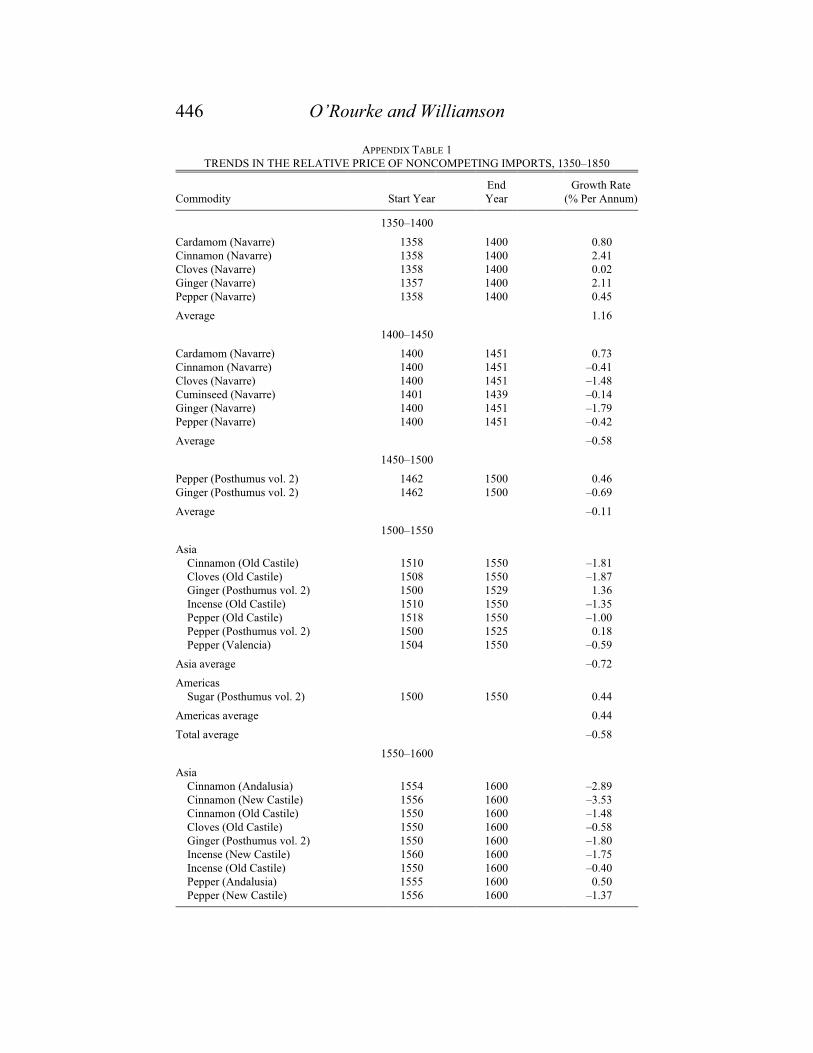
APPENDIX TABLE 1
TRENDS IN THE RELATIVE PRICE OF NONCOMPETING IMPORTS, 1350–1850
Commodity Start Year
End
Year
Growth Rate
(% Per Annum)
1350–1400
Cardamom (Navarre) 1358 1400 0.80
Cinnamon (Navarre) 1358 1400 2.41
Cloves (Navarre) 1358 1400 0.02
Ginger (Navarre) 1357 1400 2.11
Pepper (Navarre) 1358 1400 0.45
Average 1.16
1400–1450
Cardamom (Navarre) 1400 1451 0.73
Cinnamon (Navarre) 1400 1451 –0.41
Cloves (Navarre) 1400 1451 –1.48
Cuminseed (Navarre) 1401 1439 –0.14
Ginger (Navarre) 1400 1451 –1.79
Pepper (Navarre) 1400 1451 –0.42
Average –0.58
1450–1500
Pepper (Posthumus vol. 2) 1462 1500 0.46
Ginger (Posthumus vol. 2) 1462 1500 –0.69
Average –0.11
1500–1550
Asia
Cinnamon (Old Castile) 1510 1550 –1.81
Cloves (Old Castile) 1508 1550 –1.87
Ginger (Posthumus vol. 2) 1500 1529 1.36
Incense (Old Castile) 1510 1550 –1.35
Pepper (Old Castile) 1518 1550 –1.00
Pepper (Posthumus vol. 2) 1500 1525 0.18
Pepper (Valencia) 1504 1550 –0.59
Asia average –0.72
Americas
Sugar (Posthumus vol. 2) 1500 1550 0.44
Americas average 0.44
Total average –0.58
1550–1600
Asia
Cinnamon (Andalusia) 1554 1600 –2.89
Cinnamon (New Castile) 1556 1600 –3.53
Cinnamon (Old Castile) 1550 1600 –1.48
Cloves (Old Castile) 1550 1600 –0.58
Ginger (Posthumus vol. 2) 1550 1600 –1.80
Incense (New Castile) 1560 1600 –1.75
Incense (Old Castile) 1550 1600 –0.40
Pepper (Andalusia) 1555 1600 0.50
Pepper (New Castile) 1556 1600 –1.37
After Columbus 447
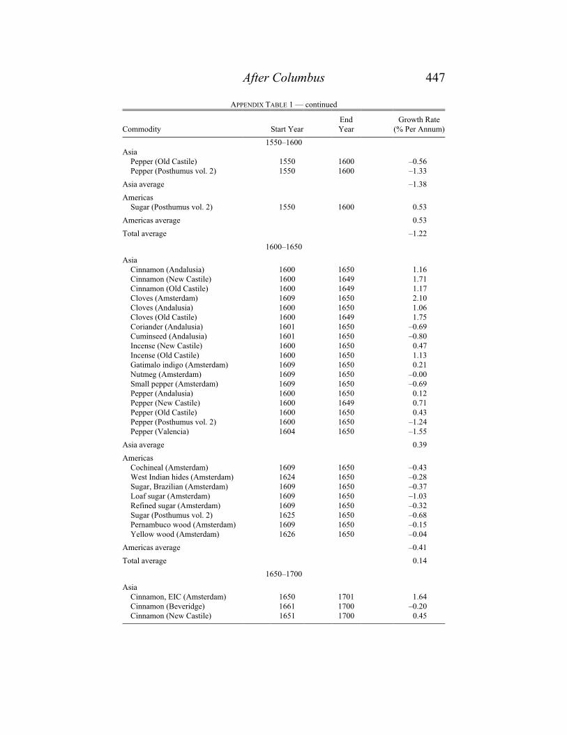
APPENDIX TABLE 1 — continued
Commodity Start Year
End
Year
Growth Rate
(% Per Annum)
1550–1600
Asia
Pepper (Old Castile) 1550 1600 –0.56
Pepper (Posthumus vol. 2) 1550 1600 –1.33
Asia average –1.38
Americas
Sugar (Posthumus vol. 2) 1550 1600 0.53
Americas average 0.53
Total average –1.22
1600–1650
Asia
Cinnamon (Andalusia) 1600 1650 1.16
Cinnamon (New Castile) 1600 1649 1.71
Cinnamon (Old Castile) 1600 1649 1.17
Cloves (Amsterdam) 1609 1650 2.10
Cloves (Andalusia) 1600 1650 1.06
Cloves (Old Castile) 1600 1649 1.75
Coriander (Andalusia) 1601 1650 –0.69
Cuminseed (Andalusia) 1601 1650 –0.80
Incense (New Castile) 1600 1650 0.47
Incense (Old Castile) 1600 1650 1.13
Gatimalo indigo (Amsterdam) 1609 1650 0.21
Nutmeg (Amsterdam) 1609 1650 –0.00
Small pepper (Amsterdam) 1609 1650 –0.69
Pepper (Andalusia) 1600 1650 0.12
Pepper (New Castile) 1600 1649 0.71
Pepper (Old Castile) 1600 1650 0.43
Pepper (Posthumus vol. 2) 1600 1650 –1.24
Pepper (Valencia) 1604 1650 –1.55
Asia average 0.39
Americas
Cochineal (Amsterdam) 1609 1650 –0.43
West Indian hides (Amsterdam) 1624 1650 –0.28
Sugar, Brazilian (Amsterdam) 1609 1650 –0.37
Loaf sugar (Amsterdam) 1609 1650 –1.03
Refined sugar (Amsterdam) 1609 1650 –0.32
Sugar (Posthumus vol. 2) 1625 1650 –0.68
Pernambuco wood (Amsterdam) 1609 1650 –0.15
Yellow wood (Amsterdam) 1626 1650 –0.04
Americas average –0.41
Total average 0.14
1650–1700
Asia
Cinnamon, EIC (Amsterdam) 1650 1701 1.64
Cinnamon (Beveridge) 1661 1700 –0.20
Cinnamon (New Castile) 1651 1700 0.45
448 O’Rourke and Williamson
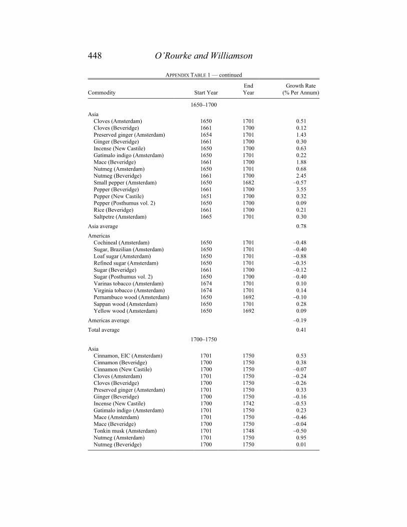
APPENDIX TABLE 1 — continued
Commodity Start Year
End
Year
Growth Rate
(% Per Annum)
1650–1700
Asia
Cloves (Amsterdam) 1650 1701 0.51
Cloves (Beveridge) 1661 1700 0.12
Preserved ginger (Amsterdam) 1654 1701 1.43
Ginger (Beveridge) 1661 1700 0.30
Incense (New Castile) 1650 1700 0.63
Gatimalo indigo (Amsterdam) 1650 1701 0.22
Mace (Beveridge) 1661 1700 1.88
Nutmeg (Amsterdam) 1650 1701 0.68
Nutmeg (Beveridge) 1661 1700 2.45
Small pepper (Amsterdam) 1650 1682 –0.57
Pepper (Beveridge) 1661 1700 3.55
Pepper (New Castile) 1651 1700 0.32
Pepper (Posthumus vol. 2) 1650 1700 0.09
Rice (Beveridge) 1661 1700 0.21
Saltpetre (Amsterdam) 1665 1701 0.30
Asia average 0.78
Americas
Cochineal (Amsterdam) 1650 1701 –0.48
Sugar, Brazilian (Amsterdam) 1650 1701 –0.40
Loaf sugar (Amsterdam) 1650 1701 –0.88
Refined sugar (Amsterdam) 1650 1701 –0.35
Sugar (Beveridge) 1661 1700 –0.12
Sugar (Posthumus vol. 2) 1650 1700 –0.40
Varinas tobacco (Amsterdam) 1674 1701 0.10
Virginia tobacco (Amsterdam) 1674 1701 0.14
Pernambuco wood (Amsterdam) 1650 1692 –0.10
Sappan wood (Amsterdam) 1650 1701 0.28
Yellow wood (Amsterdam) 1650 1692 0.09
Americas average –0.19
Total average 0.41
1700–1750
Asia
Cinnamon, EIC (Amsterdam) 1701 1750 0.53
Cinnamon (Beveridge) 1700 1750 0.38
Cinnamon (New Castile) 1700 1750 –0.07
Cloves (Amsterdam) 1701 1750 –0.24
Cloves (Beveridge) 1700 1750 –0.26
Preserved ginger (Amsterdam) 1701 1750 0.33
Ginger (Beveridge) 1700 1750 –0.16
Incense (New Castile) 1700 1742 –0.53
Gatimalo indigo (Amsterdam) 1701 1750 0.23
Mace (Amsterdam) 1701 1750 –0.46
Mace (Beveridge) 1700 1750 –0.04
Tonkin musk (Amsterdam) 1701 1748 –0.50
Nutmeg (Amsterdam) 1701 1750 0.95
Nutmeg (Beveridge) 1700 1750 0.01

After Columbus 449
APPENDIX TABLE 1 — continued
Commodity Start Year
End
Year
Growth Rate
(% Per Annum)
1700–1750
Asia
Opium (Amsterdam) 1703 1750 –0.21
Black pepper (Amsterdam) 1701 1750 0.19
White pepper (Amsterdam) 1701 1750 –0.23
Pepper (Beveridge) 1700 1750 0.27
Pepper (New Castile) 1700 1750 –0.19
Pepper (Posthumus vol. 2) 1703 1747 0.46
Rice (Beveridge) 1700 1750 –0.48
Saltpetre (Amsterdam) 1701 1750 –0.05
East Indian tin (Amsterdam) 1722 1750 –1.07
Asia average –0.05
Americas
Cochineal (Amsterdam) 1701 1750 –0.57
Cocoa, Caracas (Amsterdam) 1701 1750 –0.21
Hides, Brazilian (Amsterdam) 1701 1750 0.07
Sugar, Brazilian (Amsterdam) 1701 1750 –0.45
Loaf sugar (Amsterdam) 1701 1750 –0.14
Refined sugar (Amsterdam) 1701 1750 –0.38
Surinam sugar (Amsterdam) 1701 1750 0.30
Sugar (Beveridge) 1700 1750 –0.37
Sugar (Posthumus vol. 2) 1700 1750 0.16
Havana tobacco (Amsterdam) 1722 1750 1.89
Varinas tobacco (Amsterdam) 1701 1750 –0.22
Virginia tobacco (Amsterdam) 1701 1750 –0.06
Caliatour wood (Amsterdam) 1701 1750 0.09
Pernambuco wood (Amsterdam) 1703 1750 –0.03
Sappan wood of Siam (Amsterdam) 1705 1750 1.04
Yellow wood (Amsterdam) 1703 1750 0.28
Americas average 0.09
Total average 0.01
1750–1800
Asia
Cinnamon, EIC (Amsterdam) 1750 1800 0.08
Cinnamon (Beveridge) 1750 1781 0.73
Cinnamon (New Castile) 1750 1795 –0.62
Cloves (Amsterdam) 1750 1800 –1.41
Cloves (Beveridge) 1750 1781 –0.71
Java coffee (Amsterdam) 1750 1799 –0.58
Mocha coffee (Amsterdam) 1750 1799 –0.83
Preserved ginger (Amsterdam) 1750 1793 –0.26
White ginger (Amsterdam) 1750 1800 –0.51
Ginger (Beveridge) 1750 1781 –0.65
Gatimalo indigo (Amsterdam) 1750 1800 0.24
Java indigo (Amsterdam) 1750 1800 –0.13
Mace (Amsterdam) 1750 1794 1.37
Mace (Beveridge) 1750 1781 –1.65
Tonkin musk (Amsterdam) 1753 1800 0.59

450 O’Rourke and Williamson
Commodity Start Year
End
Year
Growth Rate
(% Per
Annum)
1750–1800
Asia
Nutmeg (Amsterdam) 1750 1800 0.91
Nutmeg (Beveridge) 1750 1781 –1.83
Opium (Amsterdam) 1750 1800 0.02
Black pepper (Amsterdam) 1750 1800 –0.51
White pepper (Amsterdam) 1750 1800 –0.66
Pepper (Beveridge) 1750 1781 –1.23
Pepper (New Castile) 1750 1799 –0.90
Pepper (Posthumus vol. 2) 1772 1800 0.99
Rice (Beveridge) 1750 1781 –1.61
Saltpetre (Amsterdam) 1750 1793 –0.46
Buoy tea (Amsterdam) 1750 1800 –1.60
Pecco tea (Amsterdam) 1758 1800 –0.11
Souchon tea (Amsterdam) 1758 1800 –1.53
East Indian tin (Amsterdam) 1750 1795 –0.93
Java yarns 'A' (Amsterdam) 1750 1797 –0.91
Asia average –0.49
Americas
Cochineal (Amsterdam) 1750 1800 –0.69
Cocoa, Caracas (Amsterdam) 1750 1800 –0.47
Surinam cocoa (Amsterdam) 1750 1800 –0.28
Surinam coffee (Amsterdam) 1750 1800 –0.11
San Domingo coffee (Amsterdam) 1757 1800 1.39
Surinam cotton (Amsterdam) 1752 1801 –0.28
Hides, Buenos Aires (Amsterdam) 1766 1800 0.08
Sugar, Brazilian (Amsterdam) 1750 1800 –0.50
Loaf sugar (Amsterdam) 1750 1800 0.75
Refined sugar (Amsterdam) 1750 1800 –0.42
San Domingo sugar (Amsterdam) 1751 1799 0.86
Surinam sugar (Amsterdam) 1750 1800 –0.24
Sugar (Beveridge) 1750 1781 –0.70
Sugar (Posthumus vol. 2) 1750 1800 0.61
Havana tobacco (Amsterdam) 1750 1782 0.76
Varinas tobacco (Amsterdam) 1750 1800 –0.83
Virginia tobacco (Amsterdam) 1750 1800 –0.35
Caliatour wood (Amsterdam) 1750 1796 –2.09
Pernambuco wood (Amsterdam) 1750 1801 0.05
Sappan wood of Siam (Amsterdam) 1750 1797 –0.77
Yellow wood (Amsterdam) 1750 1800 0.39
Americas average –0.14
Total average –0.34
1800–1850
Asia
Cinnamon, EIC (Amsterdam) 1800 1841 –0.27
Preserved ginger (Amsterdam) 1805 1851 –1.56
White ginger (Amsterdam) 1800 1847 –3.01
Black pepper (Amsterdam) 1800 1850 –2.39

After Columbus 451
68 In the case of the English data from Beveridge and the Dutch data from Posthumus vol. II, fitted
values were generated for missing observations. This generated more British and Dutch entries in
Appendix Table 1, ensuring that the overall results were not as dominated by the Spanish and Amster-
dam prices, as would have otherwise been the case.
APPENDIX TABLE 1 — continued
Commodity Start Year
End
Year
Growth Rate
(% Per Annum)
1800–1850
Asia
White pepper (Amsterdam) 1800 1850 –1.93
Saltpetre (Amsterdam) 1818 1847 –1.76
Buoy tea (Amsterdam) 1800 1850 –0.03
Pecco tea (Amsterdam) 1800 1843 –0.21
Souchon tea (Amsterdam) 1800 1850 –1.24
Asia average –1.38
Americas
Cocoa, Caracas (Amsterdam) 1800 1843 –0.92
Surinam cocoa (Amsterdam) 1800 1843 –1.22
San Domingo coffee (Amsterdam) 1800 1850 –2.00
Surinam cotton (Amsterdam) 1801 1850 –2.66
Hides, Buenos Aires (Amsterdam) 1800 1847 0.35
Sugar, Brazilian (Amsterdam) 1800 1848 –0.58
Refined sugar (Amsterdam) 1800 1851 –0.47
Surinam sugar (Amsterdam) 1800 1850 –1.06
Varinas tobacco (Amsterdam) 1800 1843 –2.94
Virginia tobacco (Amsterdam) 1800 1848 –0.83
Pernambuco wood (Amsterdam) 1801 1835 0.10
Yellow wood (Amsterdam) 1800 1835 0.44
Americas average –0.98
Total average –1.15
Sources: See the text.
1500, and so on), and computed the annual percentage rate of change between those first
and last fitted values. The series was included in Appendix Table 1 if there was at least 25
years between the first and last observations, within a given half-century. Thus, a series
would be included for the half-century 1400–1450 if, say, the first observation (and hence
fitted value) fell in 1420, and the last fell in 1448. The series would not be included if the
first observation fell in 1420 and the last fell in 1440.68
For each half-century we then calculated the mean percentage rate of change in prices.
These half-century growth rates were then cumulated to give 100-year and 300-year growth
rates in relative prices, and it is these which are used in the calculations described in the
text.
Full details of the individual price series used are given in Appendix Table 1.

452 O’Rourke and Williamson
69 Lindert and Williamson, “Revising,” table 2, p. 393, and table 3, pp. 396–97.
Appendix 2: Estimating The Growth of Europe’s“Surplus” Income, 1500–1850
National Accounting Assumptions
We assume
GDP = whP + rA + E (A1)
where w is the wage per worker (w per L), r is rent per acre (r per A), h is the labor-partici-
pation rate (L over population, P) and E is the residual income accruing to military, church,
bureaucracy, merchants, traders, and so on. Define the surplus as
S = rA + E (A2)
the income accruing to landlords and residual claimants. Assume that land is fixed, so A*
= 0. Assume also that the labor participation rate is constant, so h* = 0. Assume finally that
the residual claimants’ share of the surplus (E / S) = 0.3 and that, therefore, the landed share
of the surplus (rA / S) = 0.7. This estimate is motivated by the work of Lindert and William-
son, who document the revised Gregory King social tables figure for 1688 to be rA / S =
0.698, and the revised Joseph Massie social tables figure for 1759 to be rA / S = 0.695.69
Estimating Europe’s Demand Growth
We assume that it was the size of Europe’s surplus (S = rA + E) that determined its
demand for “exotic” commodities. While we can observe rA, we cannot observe E or its
growth (E*) prior to the nineteenth century. Thus, the three estimates in Appendix Table
2 correspond to three assumptions which, in turn, offer a range of plausibility to the S*
estimate:
A: Assume E grows like rents (rA), implying S* = r*. This characterizes the residual
class as parasitic on landlords (whom they protect, entertain, educate, fight for, sell
to, buy from, and so on);
B: Assume E grows like the economy-wide wage bill (wL), implying S* = 0.7r* +
0.3[w* + L*]. This characterizes the residual class as parasitic on the working
class and peasants. Alternatively, this characterizes the residual class as enjoying
a fixed premium above the incomes of peasants and workers, and assumes that
their numbers are in constant proportion to the working class and peasantry
(whom they police, bury, preach at, educate, oversee in the workhouses, lead to
battle, sell to, buy from, and so on).
C: Assume E grows like the urban wage bill (wLu*), implying S* = 0.7r* + 0.3[w*
+ Lu*]. This characterizes the residual class as having a fixed premium above the
incomes of the urban working class, and that their numbers are in constant propor-
tion to the urban working class. Note also that it assumes a constant wage gap
between city and farm. We tend to favor this assumption which argues that urban
growth is the engine driving imports and exports in the more advanced parts of
Europe.

After Columbus 453
APPENDIX TABLE 2
THREE ESTIMATES OF THE GROWTH IN ENGLAND’S SURPLUS, 1500–1850
(percent per annum)
Three Estimates of S*
Period A B C L* r* w* Lu*
1500–1550 –0.12 –0.11 0.02 0.60 –0.12 –0.68 1.02
1550–1600 –0.14 –0.24 –0.08 0.58 –0.14 –0.90 0.97
1600–1650 0.84 0.77 0.87 0.49 0.84 0.13 0.82
1650–1700 0.20 0.18 0.20 –0.06 0.20 0.20 0.01
1700–1750 0.16 0.18 0.31 0.26 0.16 –0.04 0.70
1750–1800 0.32 0.40 0.55 0.80 0.32 –0.20 1.30
1500–1800 0.21 0.19 0.31
1800–1850 1.13 1.49 1.90 1.65 1.13 0.67 3.02
Notes and Sources: The figures for r*, w*, and S* are deflated. The nominal wages and nominal farm
land rents for 1565–1850 are from O’Rourke and Williamson, “Heckscher–Ohlin Model.” The nominal
rents for 1495–1565 are from Clark, “Farmland,” table 6, p. 25. The deflator is the cost of living of
farm labor (Clark, “Nominal and Real Male Agricultural Wages,” table 11, pp. 43–44). The labor-force
(L) estimates are also taken from O’Rourke and Williamson, “Heckscher–Ohlin Model”; Lu is derived
by applying the share of the population urban (u) to L. The u estimates are constructed from Bairoch,
Cities, pp. 177, 179, 215–16, 221; and Hohenberg and Lees, Making, p. 84.
Growth in Real Rents for Europe’s Leaders, 1500–1800
Did the surplus in the rest of northwestern Europe center grow like that of England?
Apparently, based on the following per-annum growth rates of rent estimates from France
and Holland:
Period England France Holland Average
1500–1800 +0.21 +0.36 +0.21 +0.28
The English data are from Appendix Table 2. The French data are from Hoffman, Growth,
table 4.2, pp. 90–91; the Dutch estimates are from background data to van Zanden, “Devel-
opment,” graph 2, p. 74. The series for France and Holland both go to 1780 only. The
“Center” is an end-period weighted average of the three, using 1820 GDP weights derived
from Maddison, Monitoring, pp. 180–83.
REFERENCES
Allen, Robert C. Enclosure and the Yeoman: The Agricultural Development of the South
Midlands 1450–1850. Oxford: Clarendon Press, 1992.
Baier, Scott L. and Jeffrey H. Bergstrand. “The Growth of World Trade: Tariffs, Transport
Costs, and Income Similarity.” Journal of International Economics 53, no. 1 (2001):
1–27.
Bairoch, Paul. Cities and Economic Development. Chicago: University of Chicago Press,
1988.
Beveridge, William. Prices and Wages in England from the Twelfth to the Nineteenth
Century. Volume 1, Price Tables: Mercantile Era. London: Longmans, Green and Co.,
1939.

454 O’Rourke and Williamson
Phelps Brown, Henry, and Sheila V. Hopkins. A Perspective of Wages and Prices. London:
Methuen, 1981.
Bulbeck, David, et al. Southeast Asian Exports Since the 14th Century: Cloves, Pepper,
Coffee, and Sugar. Leiden: KITLV Press, 1998.
Chao, Kang. Man and Land in Chinese History. Stanford: Stanford University Press, 1986.
Chaudhuri, Kirti N. The Trading World of Asia and the English East India Company
1660–1760. Cambridge: Cambridge University Press, 1978.
Clark, Gregory. “Farmland Rental Values and Agrarian History: England and Wales, 1500–
1912.” Unpublished manuscript, August 1999.
______. “Nominal and Real Male Agricultural Wages, 1250–1850, and English Economic
Growth.” Agricultural History Center, Working Paper Series No. 96, University of
California, Davis (n.d.).
Crafts, N. F. R. British Economic Growth During the Industrial Revolution. Oxford: Clar-
endon Press, 1985.
Davis, Ralph. The Rise of the English Shipping Industry in the Seventeenth and Eighteenth
Centuries. London: Macmillan, 1962.
Deane, Phyllis, and W. A. Cole. British Economic Growth 1688–1959: Trends and Struc-
ture. 2nd ed. Cambridge: Cambridge University Press, 1967.
Feenstra, Robert C. “Integration of Trade and Disintegration of Production in the Global
Economy.” Journal of Economic Perspectives 12, no. 4 (1998): 31–50.
Findlay, Ronald. “Trade and Growth in the Industrial Revolution.” In Economics in the
Long View: Essays in Honor of W.W. Rostow, Vol. 1, edited by Charles P.
Kindleberger and Guido Di Tella, 178–88. London: Macmillan, 1982.
______. “The Emergence of the World Economy.” Columbia University Department of
Economics Discussion Paper No. 9596-08, April 1996.
Fisher, F. J. “Commercial Trends and Policy in Sixteenth-Century England.” Economic
History Review 10, November (1939/40): 95–117.
Flynn, Dennis O. “Arbitrage, China, and World Trade in the Early Modern Period.” Jour-
nal of the Economic and Social History of the Orient 38, no. 4 (1995): 419–48.
Flynn, Dennis O., and Arturo Giraldez. “Introduction.” In Metals and Monies in an Emerg-
ing Global Economy, edited by Dennis O. Flynn and Arturo Giraldez, xv–xl.
Aldershot: Variorum, 1997.
Frankel, Jeffrey A. “The 1807–1809 Embargo Against Great Britain.” This JOURNAL 52,
no. 2 (1982): 291–308.
Glamann, Kristof. “The Dutch East India Company’s Trade in Japanese Copper, 1645–
1736.” Scandinavian Economic History Review 15, no. 3 (1974): 351–56.
Hamilton, Earl J. American Treasure and the Price Revolution in Spain, 1501–1650. Cam-
bridge, MA: Harvard University Press, 1934.
______. Money, Prices and Wages in Valencia, Aragon and Navarre 1351–1500. Cam-
bridge, MA: Harvard University Press, 1936.
______. War and Prices in Spain, 1651–1800. Cambridge, MA: Harvard University Press,
1947.
Hirst, Paul Q., and Grahame Thompson. Globalization in Question: The International
Economy and the Possibilities of Governance. Cambridge: Polity Press, 1996.
Hoffman, Philip T. Growth in a Traditional Society: The French Countryside, 1450–1815.
Princeton: Princeton University Press, 1996.
Hoffman, Philip T., et al. “Prices and Real Inequality in Western Europe since 1500.”
Agricultural History Center Working Paper 102, University of California–Davis,
September 2000.
Hohenberg, Paul M., and Lynn Hollen Lees. The Making of Urban Europe 1000–1950.

After Columbus 455
Cambridge, MA: Harvard University Press, 1985.
Irwin, Douglas A. “Mercantilism as Strategic Trade Policy: The Anglo-Dutch Rivalry for
the East India Trade.” Journal of Political Economy 99, no. 6 (1991): 1296–314.
Jacks, David. “Market Integration in the North and Baltic Seas, 1500–1800.” LSE Working
Papers in Economic History 55/00, London School of Economics, April 2000.
Johnson, Lyman L., and Enrique Tandeter, eds. Essays on the Price History of Eighteenth-
Century Latin America. Albuquerque: University of New Mexico Press, 1990.
Jones, Eric L. The European Miracle. Cambridge: Cambridge University Press, 1981.
Krishna, Bal. Commercial Relations Between India and England, 1601–1757. London:
Routledge, 1924.
Krugman, Paul. “Growing World Trade: Causes and Consequences.” Brookings Papers on
Economic Activity, no. 1 (1995): 327–77.
Lavely, William, and R. Bin Wong. “Revising the Malthusian Narrative: The Comparative
Study of Population Dynamics in Late Imperial China.” Journal of Asian Studies 57
(August 1998): 714–48.
Lindert, Peter H., and Jeffrey G. Williamson. “Revising England’s Social Tables 1688–
1812.” Explorations in Economic History 19, October (1982): 385–408.
Ma, Debin. “The Great Silk Exchange.” In Pacific Centuries, edited by Dennis O. Flynn,
L. Frost, and A. J. H. Latham, 38–69. London: Routledge, 1999.
Maddison, Angus. Dynamic Forces in Capitalist Development: A Long-Run Comparative
View. Oxford: Oxford University Press, 1991.
______. Monitoring the World Economy 1820–1992. Paris: OECD, 1995.
______. Chinese Economic Performance in the Long Run. Paris: OECD, 1998.
______. The World Economy: A Millennial Perspective. Paris: OECD, 2001.
Marks, Robert B. Tigers, Rice, Silk, and Silt: Environment and Economy in Guangdong,
1250–1850. New York: Cambridge University Press, 1997.
______. “Maritime Trade and the Agro-Ecology of South China, 1685–1850.” In Pacific
Centuries, edited by Dennis O. Flynn, L. Frost, and A. J. H. Latham, 85–109. London:
Routledge, 1999.
McCusker, John J., and Russell R. Menard. The Economy of British America, 1607–1789.
Chapel Hill: University of North Carolina Press, 1991.
Mechner, Emily. “Pirates and Planters: Trade and Development in the Caribbean, 1492–
1680.” PhD diss., Department of Economics, Harvard University, May 1999.
Menard, Russell R. “Transport Costs and Long-Range Trade, 1300–1800: Was There a
European ‘Transport Revolution’ in the Early Modern Era?” In The Political Economy
of Merchant Empires, edited by James D. Tracy, 228–75. Cambridge: Cambridge
University Press, 1991.
Moosvi, Shiseen. “The Indian Economic Experience 1600–1900: A Quantitative Study.”
In The Making of History: Essays Presented to Irfan Habib, edited by K. N. Panikkar,
Terence J. Byres, and Utsa Patnail, 328–58. New Delhi: Tulika, 2000.
O’Rourke, Kevin H., and Jeffrey G. Williamson. “The Heckscher–Ohlin Model Between
1400 and 2000: When It Explained Factor Price Convergence, When It Did Not, and
Why.” In Bertil Ohlin: A Centennial Celebration, edited by R. Findlay, L. Jonung and
M. Lundahl. Cambridge, MA: MIT Press, forthcoming.
______. “When Did Globalization Begin?” European Review of Economic History, forth-
coming.
Phillips, Carla Rahn. “The Growth and Composition of Trade in the Iberian Empires,
1450–1750.” In The Rise of Merchant Empires: Long-Distance Trade in the Early
Modern World 1350–1750, edited by James D. Tracy, 34–101. Cambridge: Cambridge
University Press, 1990.
456 O’Rourke and Williamson
Pomeranz, Kenneth. The Great Divergence: Europe, China, and the Making of the Modern
World Economy. Princeton: Princeton University Press, 2000.
Posthumus, Nicholaas W. Inquiry into the History of Prices in Holland. 2 vols. Leiden:
Brill, 1946 and 1964.
Prakesh, Om. The New Cambridge History of India: Volume II (5): European Commercial
Enterprise in Pre-Colonial India. Cambridge: Cambridge University Press, 1998.
Reid, Anthony. Southeast Asia in the Age of Commerce 1450–1680. Volume Two: Expan-
sion and Crisis. New Haven: Yale University Press, 1993.
Steensgaard, Niels. “Freight Costs in the English East India Trade 1601–1657.” Scandina-
vian Economic History Review 13, no. 2 (1965): 143–62.
______. “The Growth and Composition of the Long-Distance Trade of England and the
Dutch Republic before 1750.” In The Rise of Merchant Empires: Long-Distance Trade
in the Early Modern World 1350–1750, edited by James D. Tracy, 102–52. Cam-
bridge: Cambridge University Press, 1990.
Truxes, Thomas M. Irish–American Trade 1660–1783. Cambridge: Cambridge University
Press, 1988.
U. S. Department of Commerce. Historical Statistics of the United States: Colonial Times
to 1970, Part 2. Washington, DC: USGPO, 1975.
Van Zanden, Jan Luiten. “The Development of Agricultural Productivity in Europe 1500–
1800.” NEHA-jaarboek 61 (1998): 66–85.
Von Glahn, Richard. Fountain of Fortune: Money and Monetary Policy in China, 1000–
1700. Berkeley: University of California Press, 1996.