After-market spare parts inventory centralization

at Sandvik Mining and Rock Technology

Thesis in partial fulfillment of the requirements for the degree ofM.Sc. in Logistics and Supply Chain Management

Faculty of Engineering LTHIndustrial Management and LogisticsDivision of Production Management

Mining and Rock TechnologyCrushing and Screening

Ruben Brückner and Jawdat Higab

University Supervisor: Johan MarklundCompany Supervisor: Miguel Rocha

June 19, 2018

Abstract

Title: After-market spare parts inventory centralization at Sandvik Mining and Rock Technology.Authors: Ruben Brückner and Jawdat HigabSupervisors: Johan Marklund, Lund University | Miguel Rocha, Sandvik ABBackground: In spare parts logistics, customers expect a high availability of spare parts fromtheir providers. It is very critical for spare parts providers to be able to satisfy customers’ de-mands. It acts as a differentiator in the customer’s buying decision. Sandvik, an engineeringcompany, is interested in improving their spare parts logistics. The case company is interested inbenefits from centralizing their inventory. They target increasing their inventory service levels,while at the same time, having a feasible solution. Inventory centralization is thought of interestbecause of the risk pooling benefits that lowers the demand uncertainty. Thus, higher servicelevels can be achieved with lower global safety stocks.Purpose: The purpose of the thesis is to investigate, model and analyze a centralized spare partsinventory solution for the case company.Methodology: Mathematical modeling of single-echelon, single item inventory systems usingVisual Basic for Applications within Microsoft Excel is a core method for this thesis. All datawere collected from the case company. Quantitative data was the dominant type of data to beused. However, qualitative data complemented the quantitative one where necessary. The thesisfollows an abductive approach but with an emphasis on deductive methods.Conclusions: Fully centralizing inventory achieves better service levels with lower safety stocksif compared to a less centralized model. However, the transportation time towards customersincreases. Customers experience availability as a performance measure. Availability includeskeeping high shelf availability and short delivery times. In this thesis, a fully centralized anda partially centralized inventory solution are further investigated. However, it is recommendedto balance the conflicting goals of providing fast delivery speed and lowering inventory. In allinvestigated models fill-rate is increased by 55% if compared to the current state. In the fullycentralized model the company can achieve a higher fill-rate and at the same time lower its in-ventory (cycle and safety stock) by 28 %. However, to achieve the same fill-rate in the partiallycentralized model, the company is expected to increase inventory by 40 % on average if comparedto the current state. Also, the case company is expected to deliver the spare-parts quicker to thecustomer in the partially centralized model when compared to the fully centralized model.Keywords: Inventory Management, Inventory Centralization, Single-Echelon Inventory Models,spare parts Logistics

Preface

This M.Sc. thesis is the result of the project work carried out in cooperation of LTHand Sandvik during the time of February — May 2018. The authors are grateful forthe opportunity to conduct this research together with the Division of ProductionManagement and at Sandvik Mining and Rock Technology. We have been supportedby numerous people in both the university and the case company. We want to high-light some of them:

Johan Marklund, we want to thank you for the time that you always took forus, for discussing problems, provisional results and report drafts. Your continuoussupervision and guidance was helpful and we always felt understood. Thank you,Miguel Rocha, Sofia Hedenström and Caroline Dahlborg for the trust in us and thecontinuous help and guidance you provided.

A lot of people have given us insights into the company and were invested intomaking our research possible: Conny Andersson, Ulf Carlqvist, Mathias Fransson,Jamie Heath, Johan Israelsson, Jonas Lindqvist, Robertino Miskolin, Tord Norden,Albin Svennelid, and Angela Wang — Thank you all very much!

We also want to thank Africa Serrano and Gustav Karlström, who not only gaveus a lot of insights but also helped us getting familiar with the organization. Last butnot least, we want to thank our fellow thesis students at Sandvik and fellow Swedishand international students at LTH that made our studies worthwhile.

— Ruben Brückner and Jawdat Higab

I

Contents

Preface I

List of Figures V

List of Tables VII

Abbreviations and Symbols VIII

1 Introduction 11.1 Background . . . . . . . . . . . . . . . . . . . . . . . . . . . . . . . . . 11.2 Company description . . . . . . . . . . . . . . . . . . . . . . . . . . . . 2

1.2.1 Product Area Crushing and Screening . . . . . . . . . . . . . . 31.2.2 Current distribution network . . . . . . . . . . . . . . . . . . . 41.2.3 Benchmark - Sandvik Coromant . . . . . . . . . . . . . . . . . 5

1.3 Problem definition and the proposed network . . . . . . . . . . . . . . 61.4 Purpose and research questions . . . . . . . . . . . . . . . . . . . . . . 71.5 Research limitations and company directives . . . . . . . . . . . . . . . 8

2 Methodology 102.1 Approach . . . . . . . . . . . . . . . . . . . . . . . . . . . . . . . . . . 112.2 Working procedure . . . . . . . . . . . . . . . . . . . . . . . . . . . . . 132.3 Data collection methods . . . . . . . . . . . . . . . . . . . . . . . . . . 14

2.3.1 Quantitative data collection . . . . . . . . . . . . . . . . . . . . 152.3.2 Qualitative data collection . . . . . . . . . . . . . . . . . . . . . 15

2.4 Research credibility . . . . . . . . . . . . . . . . . . . . . . . . . . . . . 16

3 Theoretical Framework 183.1 Order winners and qualifiers . . . . . . . . . . . . . . . . . . . . . . . . 183.2 Demand categorization . . . . . . . . . . . . . . . . . . . . . . . . . . . 193.3 Basic Inventory System . . . . . . . . . . . . . . . . . . . . . . . . . . 203.4 Supply and Demand Uncertainty . . . . . . . . . . . . . . . . . . . . . 21

II

3.5 Continuous and Periodic review of (R, Q)-based inventory systems . . 223.6 Demand during stochastic lead-times . . . . . . . . . . . . . . . . . . . 243.7 Performance measures of inventory systems . . . . . . . . . . . . . . . 243.8 Normal demand . . . . . . . . . . . . . . . . . . . . . . . . . . . . . . . 263.9 Normal demand assumption and discrete alternatives . . . . . . . . . . 273.10 Poisson distribution . . . . . . . . . . . . . . . . . . . . . . . . . . . . 283.11 Negative binomial distribution . . . . . . . . . . . . . . . . . . . . . . 283.12 Inventory level probabilities . . . . . . . . . . . . . . . . . . . . . . . . 293.13 Centralization in spare parts distribution . . . . . . . . . . . . . . . . 30

4 Modeling and Data collection 334.1 Inventory Management at the case company . . . . . . . . . . . . . . . 33

4.1.1 Lead-time . . . . . . . . . . . . . . . . . . . . . . . . . . . . . . 344.1.2 Methods of categorization . . . . . . . . . . . . . . . . . . . . . 35

4.2 Model design and execution . . . . . . . . . . . . . . . . . . . . . . . . 354.3 Data collection . . . . . . . . . . . . . . . . . . . . . . . . . . . . . . . 37

4.3.1 Demand . . . . . . . . . . . . . . . . . . . . . . . . . . . . . . . 374.3.2 Supplier lead times . . . . . . . . . . . . . . . . . . . . . . . . . 384.3.3 Crusher components list and crushers’ demand . . . . . . . . . 394.3.4 Inventory and stocks on hand . . . . . . . . . . . . . . . . . . . 394.3.5 Service measure: Fill-rate . . . . . . . . . . . . . . . . . . . . . 394.3.6 Lost demand . . . . . . . . . . . . . . . . . . . . . . . . . . . . 40

5 Analysis 415.1 Different scenarios . . . . . . . . . . . . . . . . . . . . . . . . . . . . . 41

5.1.1 Scenario 1: Fully centralized after-market demand . . . . . . . 425.1.2 Scenario 2: Partially centralized after-market . . . . . . . . . . 435.1.3 Scenario 1P: Centralized after-market and production demand 44

5.2 Identifying demand patterns . . . . . . . . . . . . . . . . . . . . . . . . 465.3 Expected inventory levels E[IL+] . . . . . . . . . . . . . . . . . . . . . 49

5.3.1 Category “increase” . . . . . . . . . . . . . . . . . . . . . . . . . 515.3.2 Category “decrease” . . . . . . . . . . . . . . . . . . . . . . . . 515.3.3 Category “same” . . . . . . . . . . . . . . . . . . . . . . . . . . 535.3.4 Integrating production . . . . . . . . . . . . . . . . . . . . . . . 545.3.5 Summary of scenario analysis . . . . . . . . . . . . . . . . . . . 55

5.4 Centralization: Factors and Performance . . . . . . . . . . . . . . . . . 565.4.1 Determining item centralization level . . . . . . . . . . . . . . . 58

III

6 Discussion about the impact of lost sales 606.1 Approaches . . . . . . . . . . . . . . . . . . . . . . . . . . . . . . . . . 606.2 Lost sales and inventory centralization . . . . . . . . . . . . . . . . . . 61

7 Conclusion 647.1 How much stock should be kept in a centralized inventory solution to

accommodate a fill rate of 95 %? . . . . . . . . . . . . . . . . . . . . . 657.2 What are the benefits/trade offs of having such a system? . . . . . . . 667.3 Can new equipment production use the centralized inventory solution

as well? . . . . . . . . . . . . . . . . . . . . . . . . . . . . . . . . . . . 667.4 How can lost sales be related to the suspected availability issues? . . . 677.5 Generalizability of the models and research results . . . . . . . . . . . 677.6 Limitations and further research . . . . . . . . . . . . . . . . . . . . . 68

Bibliography 69

Appendix: Visualization Application 73

IV

List of Figures

1.1 Product areas within Sandvik Mining and Rock Technology. . . . . . . 31.2 Crushing and Screening rock solutions (Sandvik Crushing & Screening

2018). . . . . . . . . . . . . . . . . . . . . . . . . . . . . . . . . . . . . 41.3 Current supply and distribution network. . . . . . . . . . . . . . . . . 51.4 Distribution network with a single warehouse (later on referred to as

Scenario 1) . . . . . . . . . . . . . . . . . . . . . . . . . . . . . . . . . 71.5 Overview of important parts. . . . . . . . . . . . . . . . . . . . . . . . 9

2.1 Empirical Research of operations research (Fisher 2007) . . . . . . . . 112.2 Inductive and deductive approaches to research (Woodruff 2003). . . . 112.3 Systems view on problem-solving by (Mitroff et al. 1974). . . . . . . . 122.4 Overview of thesis working procedure . . . . . . . . . . . . . . . . . . 14

3.1 Demand categorization model (Syntetos et al. 2005). . . . . . . . . . . 203.2 Single stage inventory system. . . . . . . . . . . . . . . . . . . . . . . . 213.3 Resulting sawtooth pattern of basic inventory system. . . . . . . . . . 213.4 IL and IP with R = 4 and Q = 4 (Hopp & Spearman 2000). . . . . . 233.5 Basic inventory graph under periodic review (Axsäter 2006) . . . . . . 23

4.1 Algorithm used in Analysis. . . . . . . . . . . . . . . . . . . . . . . . . 36

5.1 Data modeling for Scenario 1 . . . . . . . . . . . . . . . . . . . . . . . 435.2 Scenario 2 distribution network . . . . . . . . . . . . . . . . . . . . . . 435.3 Data modeling for Scenario 2 . . . . . . . . . . . . . . . . . . . . . . . 445.4 Distribution network integrating production. . . . . . . . . . . . . . . 445.5 Data modeling for Scenario 1P . . . . . . . . . . . . . . . . . . . . . . 455.6 Demand graphs over time of example items. . . . . . . . . . . . . . . . 465.7 Investigated items in the four-field matrix (Syntetos et al. 2005) . . . . 475.8 Overview of the results for the expected inventory levels (Normalized

inventory levels) . . . . . . . . . . . . . . . . . . . . . . . . . . . . . . 49

V

5.9 Item A: category increase . . . . . . . . . . . . . . . . . . . . . . . . . 525.10 Item B: category decrease . . . . . . . . . . . . . . . . . . . . . . . . . 535.11 Item C: ∆ = ±10 % for Scenario 1 and Scenario 1P . . . . . . . . . . . 545.12 Item D: ∆ = ±10 % for Scenario 2 . . . . . . . . . . . . . . . . . . . . 545.13 Overview of change in on-hand inventory level when integrating pro-

duction demands with the fully centralized aftermarket inventory. . . . 555.14 Reduction in on-hand inventory histogram . . . . . . . . . . . . . . . . 58

1 Appendix: Visualization View I . . . . . . . . . . . . . . . . . . . . . . 732 Appendix: Visualization View II . . . . . . . . . . . . . . . . . . . . . 74

VI

List of Tables

1.1 Product portfolio structure of Sandvik Crushing and Screening . . . . 3

3.1 Comparison of service supply chain strategies (Cohen et al. 2000). . . 32

4.1 Inputs and outputs of the tool programmed in Visual Basic for Appli-cations . . . . . . . . . . . . . . . . . . . . . . . . . . . . . . . . . . . . 35

4.2 Estimate of sea freight transit times. . . . . . . . . . . . . . . . . . . . 38

5.1 Overview of items in demand categories . . . . . . . . . . . . . . . . . 475.2 Overview of machine types and their respective spare-parts’ demand

pattern . . . . . . . . . . . . . . . . . . . . . . . . . . . . . . . . . . . 485.3 High-level comparison of actual inventory levels . . . . . . . . . . . . . 505.4 Item group representatives . . . . . . . . . . . . . . . . . . . . . . . . . 515.5 demand shape vs performance (actual versus Scenario 2) . . . . . . . . 565.6 Overview of implications of centralization decisions. . . . . . . . . . . 57

VII

Abbreviations and Symbols

definition

µ, mean demand during the lead-time [units]µd mean demand per time unit [units]µL mean supply lead-time [time unit]σ, standard deviation of demand during the lead-time [units]σd standard deviation of demand per time unit [units]σL standard deviation of the supply lead-time [time unit]DOS days of supplyIL inventory level [units]IL− back-ordered demand [units]IL+ inventory on-hand [units]E[IL+] expected inventory on hand [units]IL+

actual actual average on-hand inventory level at case company [units]Q order quantity [units]R reorder point [units]S1 service level 1, (probability of no stock-out during replenishment period)S2 service level 2, fill-rate (fraction of demand satisfied immediately from

stock)S3 service level 3, ready-rate (fraction of time with positive stock on hand)S2 actual actual service level 2 as measured by the case companyVMR Variance to Mean Ratio

VIII

definition

AM After-MarketAPAC Asia PacificAPICS American Production and Inventory Control SocietyBA Business AreaDC Distribution CentreERP Enterprise Resource PlanningIoT Internet of ThingsNA North AmericaPA Product AreaRDC Regional Distribution CentreSA South AmericaSMCL Sandvik Mining and Construction Logistics

IX

Chapter 1

Introduction

This introductory chapter describes the background of the study, introduces the casecompany along with the formulated problem, and finally discusses the delimitationsof this thesis project.

1.1 Background

According to the American Production and Inventory Control Society (APICS), in-ventory is defined as stocks or items that are used to support production (raw materialand work-in-process), support activities (maintenance, repair, and operating supplies)and customer service (finished goods and spare parts) (Pittman et al. 2016).

Supply chain management is concerned with planning, controlling and managingthe flows of materials from suppliers to customers (Axsäter 2006). Today, a significantamount of capital is tied up in inventory, therefore, it is widely recognized by topmanagement as an area with opportunities for improvement (Axsäter 2006). Inventorycan’t be isolated from other supply chain management functions as different functionscan have a direct influence on inventory, for example, purchasing often tries to buymaterial in large batches as it is more economical, at the same time, productionprefers having stocks on hand immediately to avoid long machine stoppage, also,the marketing function prefers having high finished goods inventory to provide highservice levels for customers (Axsäter 2006). Inventory management aims to balancethese different inventory goals. Along with the advances in information technology, itis now possible to efficiently manage inventory to lower costs (Axsäter 2006). The twomain reasons for keeping inventories are economies of scale and uncertainties. Theeconomies of scale are often generated by the fact that ordering in batches is more

1

economical than ordering a single unit. Uncertainties in demand along with havingvariable supply lead times create the need for keeping safety stocks (Axsäter 2006).

Spare parts logistics can be defined as a logistical system that includes the plan-ning, design, realization, and control of spare parts supply and distribution. Efficientspare parts logistics with a well-aligned strategy can differentiate a business from itscompetitors. It can add greater value to the customer beyond the primary productbenefits. This can build a long-term customer loyalty and help achieving better profitmargins. Manufacturers are expected to meet the customers’ high expectations interms of delivery of service and long-time availability of spare parts (Wagner et al.2012). Also, providing a high service level will result into very few lost sales (Axsäter2006).

Through multiple case studies, (Wagner et al. 2012) conclude that companies whoare performing well in the field of spare parts logistics most often had a central storage,while keeping fast-moving items available closer to the customer. Long-term contractsare established and selective storage is decided based on spare parts criticality andvalue. Threats to the after-market spare parts business are identified as direct salesby suppliers and copied parts, especially from the Asian markets (Wagner et al. 2012).

One of Sandvik’s sub-companies (Crushing and Screening) has perceived the im-portance of spare parts logistics and the potentials for improving the current logisticssystem. This master thesis focuses on investigating and analyzing three centralizedinventory solutions for Sandvik’s Crushing and Screening spare parts distributionnetwork.

1.2 Company description

Sandvik is a global engineering company in “mining and rock excavation, metal-cuttingand materials technology” (Sandvik 2018).

Sandvik’s Product Area (PA) Crushing and Screening, part of the Business Area(BA) Sandvik Mining and Rock Technology (SMRT), develops, produces and sellsequipment for size reduction and sorting of rock material. Different industrial so-lutions such as excavator-like “breaker” machines, sorting and conveying systems“screens”, as well as stationary and mobile crushing units are offered. Their productfamily of stationary crushers is used in countries around the world. The after-marketlogistics for PA Crushing and Screening is currently being handled by one of the eightother PAs in SMRT called Parts and Services. The PA Crushing and Screening isundergoing a strategic alignment project to gain better control over their logistics

2

operations and rely less on the Parts and Services organization. This comes alignedwith Sandvik’s high-level strategy of decentralizing their PAs. Parts and Services willthen continue to take care of after-market sales and customer service, while inventorycontrol and distribution will be entirely managed by Crushing and Screening. Moredetails about Sandvik units and products hierarchy is shown in Figure 1.1. In thismaster thesis Sandik Crushing and Screening and Parts and Services will be referredto as the case company and the intermediate organization, respectively.

   Organizational Chart

Sandvik Group

MachiningSolutions

(SMS)

Mining and RockTechnology

(SMRT)

MaterialsTechnology

(SMT)

MechanicalCutting Rock Tools Drilling Automation

Loading andHauling Exploration Crushing and

Screening Parts andServices

Breakers StationaryCrushers

Mobile Crushers

Prod

uct F

amily

Prod

uct A

rea

Busi

ness

Are

aG

roup

Figure 1.1: Product areas within Sandvik Mining and Rock Technology.

1.2.1 Product Area Crushing and Screening

As presented by the president of the Product Area (PA) Crushing and Screening(Svensson 2018), they offer advanced and proven solutions for any-size reductionprocess whether it is stationary or mobile. The equipment is engineered for maximumproductivity with comprehensive life cycle services. The product portfolio includesthree categories shown in Table 1.1.

Table 1.1: Product portfolio structure of Sandvik Crushing and Screening

Type Use Case

Breakers Applied in construction units to break rocks.Mobile Crushers Mobile unit with crushing and screening equipment mounted on it.Stationary Crushers Large non-movable and connected with screens and feeders.

3

Each category has a wide range of equipment that is used for rock crushing andprocessing. Figure 1.2 shows an overview of an exemplary mining site with Sandvik’ssolutions. Generally, the purpose and the type of rock define the processing equipmentthat should be used.

Figure 1.2: Crushing and Screening rock solutions (Sandvik Crushing & Screening2018).

1.2.2 Current distribution network

The distribution network for spare parts (see Figure 1.3) is currently run by twodifferent types of entities, the central network and the sales areas:

• Central Network. Central distribution centers in Western Europe and regionaldistribution centers on every other continent are operated by the logistics func-tion of the intermediate organization. The distribution centers belong partlyto the after-market function of the entire business area. Recently, one centraldistribution center has been transitioned to a new warehousing site managed bythe case company.

• Downstream Organizations. Entities are most often responsible for the businessin one country, where inventory is held in non-standardized ways. Some entitiesrely on inventory management principles, while others might build stock basedon recent sales of new equipment and promises made towards end-customers.

The spare parts are partly produced by the production sites which are also assemblingthe new equipment, others are supplied externally.

4

Downstream organizationIntermediate organizationUpstream organization

Suppliers Production -Svedala 

DC -Svedala

DC -Netherlands

RDC -Chicago

RDC -Johannesburg

RDC -Sigapore

RDC -Perth

RDC -Brisbane

M SalesAreas

N EndCustomers

Figure 1.3: Current supply and distribution network.

1.2.3 Benchmark - Sandvik Coromant

Sandvik Coromant, another company in the Sandvik group, is active in the toolsand inserts business for metal cutting applications such as turning and milling. Theinformation in this section is mainly based on a telephone interview with a personresponsible for Supply and Production Planning at Sandvik Coromant (Israelsson2018). Inserts are small parts of a cutting tool that are worn off during use. Thesesmall yet expensive parts are regularly bought, have a high stock availability tar-get and are shipped to customers over night. Insert holders are sold less often, alsohave a high stock availability goal but are shipped within 72 hours, often within 24hours. The distribution network of the benchmark company consists of four distri-bution centres (DCs) located in four different geographical regions (more exactly inthe Netherlands, North America, China and Singapore). The mode of transportationemployed between the DCs is air-freight, for which fixed volumes are contracted fromcarriers serving airports close to the DCs. Supply into the distribution network anddeliveries to customers are often road-based, but air freight is used when necessary.

By that, Sandvik Coromant offers its customers consistently short lead-times andmaintains low inventory levels by pursuing a centralized distribution strategy in con-junction with express freight. Customers do not need to keep significant inventoriesand can rely on timely deliveries. Because insert holder production is designed forachieving short lead-times even for many customized products, customers can getthose specific tools often in less than two weeks.

5

1.3 Problem definition and the proposed network

The case company is exposed to changing market conditions. Demand has beenchanging considerably resulting in a need for inventory adjustments. Recently, thedemand has been increasing which has depleted inventories in parts of the after-marketsupply chain. This has resulted in decreased trust in the after-market capabilitiesof the case company by the downstream organization and end-customers. The mainobjective of this thesis is to develop a generic inventory model that can help to improvethe after-market distribution network. For a sample of items a comparison is madebetween current and future inventory performances.

In comparison with other business areas inside Sandvik Group, the case companyoffers opportunities for improvement with regards to logistics cost. The company iswondering whether the logistics system for Stationary Crusher spare parts could beorganized similar to the logistics system at the benchmark company Sandvik Coromant(see Section 1.2.3). Even though the product range is quite different, it is to beevaluated whether there are possible learnings to be transferred.

The after-market business model for the case company is considered to be differ-ent than the benchmark company. Spare part logistics differs from the logistics forconsumables. The quantity and frequency of spare parts order lines are often low. Incontrast, consumables at Sandvik Coromant have significant material flows.

Sandvik Crushing and Screening identifies some of their crushers as Core Products(or core machinery equipment). Core equipment are defined based on sales, profit,installed base and life cycle potential. Core equipment are as follows: Cone Crushers,Jaw Crushers and Screens. Each equipment consists of a large amount of components.Sandvik categorizes components for Cone crushers into four main types:

1. Wear Parts: Parts that are in direct contact with rocks and wear off duringusage. Can be characterized as heavy, bulky and non-stackable.

2. Spare Parts: All nuts, bolts and small parts that have no proprietary drawing.

3. Key components: Strategic and important components that are Sandvik spe-cific.

4. Major components: Large and heavy Sandvik specific parts that shapes thecrusher.

The crushing products are recognized by the case company to have the highestpotentials for improvement. Among the crushing products, cone crushers are chosendue to their popularity among customers. They come in different sizes and dependingon the customers’ requirements slight technical modifications are present. The case

6

company is interested in improving the inventory management for their strategic com-ponents, thus, this master thesis will focus on two main categories, Major componentsand Key components (see Figure 1.5). According to the case company, strategic itemsare constantly driving the after-market sales, also, these items form a critical need forthe crusher to function. Furthermore, the study will be conducted on an item level.

It has been directed by the management to start by modeling a single locationwarehouse. This thesis will, as a first option, consider an inventory model that relieson a single DC. The DC will supply end-customers with after-market spare parts (seeFigure 1.4).

Supplier

Production -Svedala 

N EndCustomers

S2 > 95 %Global Warehouse

Figure 1.4: Distribution network with a single warehouse (later on referred to asScenario 1)

Additionally, the company showed concerns regarding the rate of spare part salesper sold capital equipment varying greatly among different sales areas. It is suspectedthat this is mostly due to a difference in availability of spare parts toward the cus-tomer. The role of lost demand in connection with the analysis of the thesis will bediscussed separately.

1.4 Purpose and research questions

The purpose of this thesis is to model and analyze a centralized inventory solutionfor the case company’s aftermarket distribution system. Thus, the research questionsare:

1. How much stock should be kept in a centralized inventory solution to accom-modate a fill rate of 95 %?

2. What are the benefits and trade-offs of having such a system?

3. Can new equipment production use the centralized inventory solution as well?

4. How can lost sales be related to the suspected availability issues?

7

1.5 Research limitations and company directives

The aim of this section is to specify the the scope and limitations. A number of differ-ent limitations were determined together the case company. The following limitationsare considered to limit the scope of the research. However, the limitations are thoughtto be able to deliver generalizable findings. The main limitations are as following:

• Demand data should be based on end customer sales orders only.

• The study should only consider a sample of key and major components for conecrushers.

• Target fill-rate in the virtual warehouse should be 95 %.

8

1. Not considered

2. Key component

3. Key component

4. Major component

5. Major component

6. Key component

7. Not considered

8. Not considered

9. Not considered

10. Key component

11. Key component

12. Not considered

13. Not considered

14. Not considered

15. Key component

16. Key component

17. Key component

18. Not considered

19. Key component

20. Not considered

21. Not considered

22. Major component

23. Not considered

24. Key component

25. Key component

26. Not considered2.2.1. Sectional view of a cone crusher

26

25

24

2322

21

20

18

19

17

16

15

1412

13

11

10

6

7

8

9

4

5

2

1

3

Cone Crusher CH series

1 Spider seal2 Mainshaft sleeve3 Concave ring4 Topshell5 Bottomshell6 Dust seal ring7 Retaining ring8 Locating bar9 Dust collar10 Pinionshaft11 Pinionshaft housing12 Hydroset piston13 Hydroset cover14 Chevron packing15 Step bearing components16 Eccentric bushing

2. Equipment description

16 Copyright © SandvikS 223.1318 - 1 en-US 26/04/2016 09:40:34

Figure 1.5: Overview of important parts in aCone Crusher with major components and key components highlighted as per definition by

the case company.

9

Chapter 2

Methodology

This chapter discusses different types of methodologies used in operations research.It describes the approach that is used in this thesis and the working procedure thatis followed. The data collection conducted and the criteria of research credibility aredescribed and reflected upon.

Organizations have become more and more complex since the industrial revolu-tion and along with division of labour and specialization. Along this development, itbecomes more difficult to allocate resources for activities in an effective and efficientway for the whole organization. The ambition to find answers to questions of resourceallocation builds the basis for Operations Research (Hillier & Lieberman 2001). Dif-ferent frameworks have been published as attempts to improve the empirical base ofoperations research in relation to research methodology. One interesting frameworkhas been developed by (Fisher 2007) which presents a two-by-two matrix (Figure 2.1)for empirical research in this field. The author distinguished four kinds of researchmethodologies depending on the goal of the research (descriptive or prescriptive) andthe level of real world interaction (highly structured or less structured). This masterthesis is discussing a highly structured data and algorithms that are directly relatedto the surrounding environment in order to provide a solution for a well defined prob-lem, thus this thesis mainly falls under the Engineering category according to Fisher’smatrix.

Also according to (Woodruff 2003), two research approaches, that any researchfollows when contributing to a field of knowledge, can be categorized. The categoriesinclude the inductive approach and the deductive approach (Figure 2.2). The in-ductive approach tries to generalize from a specific observation such as interviews todescribe a phenomenon. On the other hand, the deductive approach relies on logical

10

Figure 2.1: Empirical Research of operations research (Fisher 2007) .

Phenomena

DataCollection

Description

SubstantiveTheory

FieldVerification

FormalTheory

LiteratureReview

Inductive qualitative approach

Deductive quantitative approach

Figure 2.2: Inductive and deductive approaches to research (Woodruff 2003).

structures and certain preconditions in order to make true claims. Most parts of thismaster thesis rely on logical structures, literature reviews and actual data but alsowith the presence of some interview to understand the description of specific prob-lems. Thus, this master thesis can be categorized as a mixture of both approaches(also known as abductive approach (Kovács & Spens 2005)), but with an emphasison the deductive approach.

2.1 Approach

Quantitative research tries to discover solutions for real problems (Mitroff et al. 1974).This theory is established upon being able to separate subsystems through systemboundaries, as do most of engineering disciplines. The authors describe the researchprocess in four main elements:

11

(I) Reality: The origin of ideas and the starting point of research.

(II) Conceptual model: An abstract model that is related to reality.

(III) Scientific model: More formal terms with more formal relations between param-eters (e.g. mathematical equations).

(IV) Result: Problem solving is applied to the well structured model in ordered toget the solution (e.g. linear programming).

If the four main elements of the research process result in a solution that is accuratefor the problem question, an implementation process will close the loop and connectback to the main element which is reality (Mitroff et al. 1974).

I Reality ProblemSituation

II Conceptual 

Model

III Scientific

Model

Conceptualization Modeling

IV

Solution

Model SolvingImplementation

Validation

Feedback

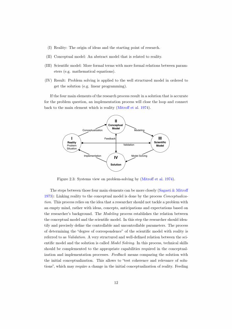
Figure 2.3: Systems view on problem-solving by (Mitroff et al. 1974).

The steps between those four main elements can be more closely (Sagasti & Mitroff1973): Linking reality to the conceptual model is done by the process Conceptualiza-tion. This process relies on the idea that a researcher should not tackle a problem withan empty mind, rather with ideas, concepts, anticipations and expectations based onthe researcher’s background. The Modeling process establishes the relation betweenthe conceptual model and the scientific model. In this step the researcher should iden-tify and precisely define the controllable and uncontrollable parameters. The processof determining the “degree of correspondence” of the scientific model with reality isreferred to as Validation. A very structured and well-defined relation between the sci-entific model and the solution is called Model Solving. In this process, technical skillsshould be complemented to the appropriate capabilities required in the conceptual-ization and implementation processes. Feedback means comparing the solution withthe initial conceptualization. This allows to “test coherence and relevance of solu-tions”, which may require a change in the initial conceptualization of reality. Feeding

12

those results into reality is then considered the Implementation of the problem-solvingprocess.

In this master thesis these steps have been put to use as follows:

(a) Conceptualization: The current supply chain network is characterized by nu-merous legal and organizational entities and stocking locations with mostly nostandardized decision making. Theory as well as practices at a sister companysuggest that there may be benefits from centralization of inventory locations.

(b) Modeling As the case company is undergoing a change that affects operations,it is important to construct a basic model for inventory control that utilizes theavailable data. The model should be adaptable to match reality more closely inthe future. Therefore, the investigation first concentrates on a single-echelon,single item model.

(c) Validation: The comparison of the current supply chain network with the scien-tific model chosen leads to the generation of more realistic scenarios includingfive distribution centres, one per geographic business region.

(d) Model solving: An algorithm is designed and implemented in Visual Basic forApplications (Microsoft Excel) to evaluate and optimize the results of the thescientific model.

(e) Feedback: Results coherence and alignment with the conceptual model formedthe importance of this step.

(f) Implementation: Presentation of the visualized model outcome and collectionof feedback from practitioners at the case company. Based on this, the abilityto implement the solution was discussed.

2.2 Working procedure

The working procedure for this study follows an approach similar to the one by(Mitroff et al. 1974) as described in Section 2.1. Figure 2.4 provides an overviewof the working procedure.

13

01

02

03

04Understand the

distribution network reality

Build a conceptual distribution model

Analyse findings and dilemmas and reflect on reality

Rely on scientific models and data collection to optimize inventory

Figure 2.4: Overview of thesis working procedure

The first step is to understand the real inventory system situation, formulate theproblem and collect initial data to help developing thoughts for a conceptual model.Then a scientific model is built. It relies on data collection as inputs and validationtechniques to confirm correspondence with the real system. Then, the scientific modelsolving offers initial results that are taken into further analysis. The results are thenanalyzed and reflected into reality in order to understand how the implementation ofthis model will influence the real situation. The analysis also includes testing of theconceptual model to make sure that it is aligned with theory and results.

2.3 Data collection methods

(Flynn et al. 1990) describe a step-wise approach to Operations Management Re-search. As a first step, it should be contemplated whether the endeavour entailstheory building or theory verification. Afterwards, a research design is to be cho-sen. Furthermore, a data collection method is to be defined, for which they mentionamong others “historical archive analysis, observation, interviews, questionnaires andcontent analysis”. Gathering this data is called “implementation” in their terminology,followed by data analysis. Then, a publication is to be produced and published.

Various data collection techniques can be used in logistics. Both quantitativeand qualitative data collection methods are present. Quantitative techniques aremost likely connected to numerical data and specifically to numerical analysis (Spens& Kovács 2006). On the other hand, qualitative data collection methods gathernon-numerical data. The data collection method does not necessarily conclude theresearch type (quantitative or qualitative) as quantitative data can be used to beanalyzed qualitatively and conversely, too (Spens & Kovács 2006).

14

2.3.1 Quantitative data collection

Archived data has no bias, as the data provider is not aware of the observation process.However, the desired data might be hard to obtain as the environment is not under thecontrol of the observer. Historical archive analysis makes use of physical traces andarchives, for example reports that firms are required to file (Flynn et al. 1990). Thismaster thesis relies heavily on the case company data records. Data is documented andpublished using different software packages. As part of accessing the data, responsibledata stakeholders are involved into granting access to the researchers. Data is alsofragmented across different software packages and IT systems, therefore, the authorsreceived administrative instructions for this data collection method.

2.3.2 Qualitative data collection

The interview is one of the most popular methods in qualitative research. It often issemi-structured, i.e. there is a predefined set of topics that are planned to be cov-ered. It nevertheless is open and the interviewer can react to previous responses andchange the course of the interview. The environment in which the interview is heldas well as the briefing before and debriefing after an interview play an important rolein creating a successful information exchange. Interview questions should be askedusing the language of the interviewee (Kvale 2007). According to (Flynn et al. 1990)there are two main types of interviews; (1) structured interviews and (2) ethnographicinterviews. Structured interviews often follow a standard form of questions that isscripted, however, other questions maybe asked based on the direction of the conver-sation. This type of interview allows for some comparison between the intervieweeswhile keeping the focus on the depth of the personal interview. On the other hand,ethnographic interviews follow a hierarchy of questions that begins with a generalquestion, by then, the questions are framed based on the interviewees answers. Thequality of both interview types further improve with transcriptions, because the re-searcher is not distracted by taking detailed notes (Flynn et al. 1990). In this masterthesis, a structured interview is held in order to collect qualitative data regarding thelost demand section. The interviewee was briefed with the interview questions priorto the interview. During the interview, the interviewer was not the one taking notes,rather, focused on the depth of the interview. It is worth noting that a challengingissue regarding this part can be the possibility for holding multiple interviews withsimilar stakeholders in order to gather more reliable qualitative data.

15

2.4 Research credibility

Research quality can be assessed through different factors. It has been pointed outthat quantitative research is a method of the positivist paradigm (Näslund 2002).Positivists research is formed after mechanisms used in natural science. Researchfollowing the positivist method can be described as “good” if the following four criteriaapply (Näslund 2002):

1. Internal validity

2. External validity

3. Reliability

4. Objectivity

Internal validity: Internal validity is concerned with the degree of how good thefindings are in mapping the phenomena, in other words, how good the model isin presenting reality (Näslund 2002). In this thesis, a well defined theory (singleechelon inventory optimization) is being used, therefore the internal model validityhas already been tested across many years of previous research. The input data wascontinuously cross-checked with stakeholders to confirm an accurate representation ofreality. Therefore, it is argued that the internal validity is high.

External validity: External validity is concerned with the outer space of the re-search and how well it is applicable in similar situations (Näslund 2002). As in thismaster thesis, the inventory being modelled is specifically done for spare parts supplychain distribution and the findings are in line with literature recommendations. Thescientific model is general and was implemented in an algorithm without significantconstraints. The algorithm can be used in similar settings and does not have to followthe same assumptions that have been used in the project work (e.g. replenishmentquantity Q: the calculations in this report are based on Q = 1, but the model hasbeen designed to work with any quantity).

Reliability: Research reliability includes the degree of which the finding can berepeated or reproduced (Näslund 2002). Regarding the scientific model in this masterthesis it has been further tested manually and produced the same numbers for thesame inputs. Furthermore, the inputs are thought to be the main challenge in thisthesis as data collection process relied on gathering data, cleaning data from outliersand validating it for usage. The model consistently produces the same output for thesame inputs. Thus, the reliability is considered to be high.

Objectivity: Objectivity is concerned with the research bias and how to developbias-free findings (Näslund 2002). This research relied on mathematical modeling thatis well defined in literature, the collected data has no influence over the mathematicalmodel design, rather, the mathematical model objective is to prescribe a solutionfor the real situation and the results are then analyzed and understood without any

16

directives. For some parts of this thesis, where the researchers discuss the issue oflost sales, qualitative data collection was relied on to gather further understandingthat was not acquired from archived data, therefore, a bias toward the intervieweecould be possible regarding this part. The statements from the interview have beenput into context and it has been made clear that their validity is restricted to thegeographical responsibility of the interviewee. As the general recommendation is tofurther look into this matter, this possibility of a bias is not considered severe.

Closely connected to the question of research credibility is the selection of andreflection on the sources. Source criticism has its roots in the historical sciences.According to (Thurén 2003), source criticism is not possible based on a “recipe” only,but requires (1) knowledge, (2) attention to small things, (3) thoughtfulness, (4)imagination, and (5) awareness of one’s own prejudices. Based on those prerequisites,it is possible to attempt an evaluation of a source regarding four dimensions (looselytranslated from (Thurén 2003)):

1. Authenticity 2. Time 3. Dependency 4. Tendency

Authenticity means that the source has not been forged. All sources used in thisthesis are either based on genuine internal information (company records, personalmeetings and conference calls) at the case company or literature from recognizedjournals and publishers when it comes to theory. Therefore, authenticity is achievedby relying on subject authorities (well reputed scientific journals) and representativesappointed by the principal at the case company.

Time relates to the fact that the human memory changes over time. Companyrecords have been used to provide evidence regarding past developments. Other in-formation related to the current state at the case company, which makes the factortime unproblematic.

Dependency considers rumors and different kinds of influences. Personal sourceshave been contacted based on directives or multiple referrals from previously estab-lished contacts. In some cases, only one source was used, however care was taken notto consider information that might have been influenced by dependency. The mainoutcomes of the thesis are based on scientific models and archival records, whichmakes a possible dependency less impactful.

Tendency means that sources that are affected by the research are less trustworthythan impartial sources. Company employees could have been biased to present theirperformance or the state of a specific part of the organization different from reality.The interests of stakeholders have been reflected upon in order to prevent an adverseeffect on the credibility of the research and its conclusions. No potential of significantinfluence of the research outcome due to tendency has been identified.

17

Chapter 3

Theoretical Framework

First, a brief introduction to order qualifiers and order winners is provided. Then,a basic inventory system under certainty is described. The influence of supply anddemand uncertainty and the role of safety stock are then introduced. Furthermore,the steady-state nature of inventory models and the crucial role of the lead-timedemand are touched upon. The general function of the probability distributions of thelead-time demand, inventory levels, and how those are related to basic performancemeasures of inventory systems are described. After establishing these fundamentals,closed-form expressions and scientific findings based on the popular assumption ofNormal distributed demand are recapitulated. Furthermore, implications of using theNormal distribution are compared to using discrete demand distributions, such as thePoisson distribution and the Negative binomial distribution.

3.1 Order winners and qualifiers

Hill & Hill (2009) introduce the concept of distinguishing customer desires into orderqualifiers and order winners in their Framework for linking corporate objectives andoperations and marketing strategy development :

Qualifiers “get a product into a marketplace [...] and keep it there” – shouldthe company not manage to deliver this attribute satisfactorily, this leads to losingcustomers; some qualifiers are especially order-losing sensitive and should thus becarefully considered. Order-winners then are used to compare different offers that areunder consideration due to the fulfillment of the qualifiers.

The importance of one qualifier or order winner might change depending on thetime and market as well as growth and new market entry aspirations. Price and

18

delivery speed are two prominent examples, which illustrate that those attributes arenot independent but rather often involve trade-off situations.

They furthermore present examples of attributes that often are important quali-fiers or order winners, a selection of which will be briefly introduced.

• price: most often, price is perceived as a qualifier: potential suppliers areshortlisted based on whether their offer lies in a reasonable price range comparedto their competitors. The lowest bidder does usually not get the order withoutany other factor considered.

• delivery reliability: meeting the promised delivery date is often consideredan order qualifier. However, it is only experienced once the order is placed. Insome businesses, this criterion is classified as being order-losing sensitive.

• delivery speed: is often considered an order winner.

• quality conformance: is often considered an order qualifier, as customersexpect the product to adhere to its specifications.

3.2 Demand categorization

Syntetos et al. (2005) suggest that the use of forecasting methods for spare partsdemand should be undertaken using their four-field decision matrix. It employs twodimensions: the average demand interval and squared coefficient of variation (whichare denoted here with ADI and CV 2, respectively). Cut-off values have been definedbased on goodness-of-fit tests with large data-sets of real demand patterns againstdifferent forecasting methods.

Even though this categorization was originally intended for choosing the optimalmodel to forecast future demands (Syntetos et al. 2005), it will hereafter only be usedto present a structured overview of the demand patterns present at the case company(see also limitations regarding forecasting in Section 1.5). The four classes of demandas shown in Figure 3.1 are called (1) smooth, (2) intermittent (but not very erratic),(3) lumpy, (4) erratic (but not very intermittent).

The average demand interval ADI is, different from the proposed forecasting pro-cedure, not updated based on exponential smoothing (also, it was originally denotedwith p Syntetos et al. (2005)). Inter-demand intervals are considered if there havebeen periods with no recorded demand that are followed by a period with non-zerodemand. This means that an item with only one demand period recorded can havedifferent values for their ADI. If the only non-zero demand period occurs in the veryfirst period considered, the interval between the zero-th period and the first periodis considered as 1. If in the opposite case, the only non-zero demand period is in the

19

Figure 3.1: Demand categorization model (Syntetos et al. 2005).

most recent period considered, the total number of periods considered is recorded asADI. Thus, when put into practice, such cases have to be considered carefully. Thesquared coefficient of variation CV 2 is in this context defined as in (3.1).

CV 2 =

(standard deviation of demand sum in non-zero demand periodarithmetical mean of demand sum in non-zero demand period

)2

(3.1)

The matrix model distinguishes four different demand types with rather ambigu-ous names. It is intuitive to understand that smooth demand occurs in (nearly)every period and is fairly predictable regarding the number of demanded items. Incontrast, lumpy demand exhibits demand not in every period and the amount of de-manded items varies considerably. The classes intermittent and erratic might bothappear more random to the observer but differ in the source of the demand variability:intermittent demand is mostly characterized by periods of no demand but does notexhibit high variability in the demand sum of a period. This is on the other hand themajor source of demand variability of erratic demand, which in turn does not have asmany periods with no demand (Ferrari et al. 2006). That being said, it is likely thatNormal demand assumption based inventory management systems perform well forsmooth demand but are less accurate with erratic, intermittent and lumpy demand.

3.3 Basic Inventory System

The following remarks on inventory management and most of the notation buildson the book Inventory Control (Axsäter 2006). Figure 3.2 shows a basic inventorycontrol system.

20

Figure 3.2: Single stage inventory system.

Under constant demand and constant lead-times, orders can be placed so that areplenishment arrives exactly when stock has depleted to zero. This behavior resultsin the basic sawtooth pattern, which can be observed in Figure 3.3.

Figure 3.3: Basic inventory graph under constant demand rate and order quantities.Source Axsäter (2006)

In this basic case, all demand is satisfied directly from stock, as replenishmentsarrive in the time instant when the stock level reduces to zero. It could however bebeneficial to let customers wait. In this case, the stock level decreases below zero.

3.4 Supply and Demand Uncertainty

In industrial inventory systems, the underlying assumptions of the aforementionedbasic model do not apply: Demand is seldom constant or deterministic; supply uncer-tainties add on to the complexity of inventory systems in reality. Therefore, inventoryis oftentimes held in addition to the turnover stock seen in Figure 3.3. This type ofinventory is called safety stock.

More general inventory models consider back-orders: If there is no stock on handwhen a customer demand materializes, customers wait to receive the item. In contrastto models in which consequences of back-orders are described by a cost factor, thechosen model considers full back-ordering under an availability constraint.

There are two possible generic states of an inventory when a customer arrives:

21

either there is stock available or there is not. It is the most intuitive way to think ofinventory as physical goods that are available. However, customer demands that havenot been satisfied yet (backorders) and replenishments that have not arrived yet haveto be considered as well. Those three elements are necessary to define two indicatorsof an inventory system: The inventory position IP and the inventory level IL.

The inventory position IP is the basis for ordering decisions of the inventorysystem and defined as in (3.2).

IP = physical stock on hand + replenishments outstanding− backorders (3.2)

When evaluating the inventory performance (e.g. in terms of holding and back-ordering costs), the inventory level IL has an important role. It is defined similarto the inventory position IP but does not consider replenishments outstanding, asshown in 3.3.

IL = physical stock on hand− back orders (3.3)

Hence, if there is stock on hand, IL > 0 – if customer demand is backordered,IL < 0.

From here on, we are using the following notation for simplicity: stock on hand isdonated with IL+, and back orders are denoted with IL−. More formally, they canbe defined as in (3.4) and (3.5).

IL+ = max(IL, 0) (3.4)

IL− = max(−IL, 0) (3.5)

3.5 Continuous and Periodic review of (R, Q)-based

inventory systems

When the reorder-quantity Q is fixed, a common inventory management policy is the(R, Q)-policy. That is, when the inventory position decreases to the reorder pointR, a replenishment of Q units should be requested. A special case of this policy isthe (S − 1, S)-policy or base-stock policy, i.e. Q = 1 and R = S − 1. Every timethe inventory position IP falls to or below R, a new replenishment is requested.An exemplary pattern of how the inventory level IL and IP can develop in an (R,Q)-system subject to discrete unit demand can be seen in Figure 3.4.

22

76

FIGURE 2.6Net inventory andinventory position versustime in the (Q, r) modelwith Q = 4, r = 4

Part I The Lessons ofHistory

9,-------------------,Q+r 8

765 1-L..-+---'~---'_r_----L"1_--~++--'-I--_I

r 43 I-----I..,.------,..,.--+l.---r-+--L-,-----j21 1-----''-r--l-'....--4----I.~----J_,__+__I

OI-----4+---l..rj-------h-IH-1

-2 0 2 4 6 8 10 12 1416 1820222426283032

Time

-- Inventory Position

- Net Inventory

immediately jumps to r + Q and hence never spends time at level r.) After a (constant)lead time of .e, during which stockouts might occur, the order is received. The problemis to determine appropriate values of Q and r.

As Wilson (1934) pointed out in the first formal publication on the (Q, r) model,the two controls Q and r have essentially separate purposes. As in the EOQ model, thereplenishment quantity Q affects the tradeoff between production or order frequencyand inventory. Larger values of Q will result in few replenishments per year but highaverage inventory levels. Smaller values will produce low average inventory but manyreplenishments per year. In contrast" the reorder point r affects the likelihood of astockout. A high reorder point will result in high inventory but a low probability of astockout. A low reorder point will reduce inventory at the expense of a greater likelihoodof stockouts.

Depending on how costs and customer service are represented, we will see that Qand r can interact in terms of their effects on inventory, production or order frequency,and customer service. However, it is important to recognize that the two parametersgenerate two fundamentally different kinds of inventory. The replenishment quantity Qaffects cycle stock (Le., inventory that is held to avoid excessive replenishment costs).The reorder point r affects safety stock (i.e., inventory held to avoid stockouts). Notethat under these definitions, all the inventory held in the EOQ model is cycle stock, whileall the inventory held in the base stock model is safety stock. In some sense, the (Q, r)model represents the integration of these two models.

To formulate the basic (Q, r) model, we combine the costs from the EOQ and basestock models. That is, we seek values of Q and r to solve either

or

min {fixed setup cost + backorder cost + holding cost}Q,r

min {fixed setup cost + stockout cost + holding cost}Q,r

(2.31)

(2.32)

The difference between formulations (2.31) and (2.32) lies in how customer service isrepresented. Backorder cost assumes a charge per unit time a customer order is unfilled,while stockout cost assumes a fixed charge for each demand that is not filled from stock(regardless of the duration of the backorder). We will make use of both approaches inthe analysis that follows.

Figure 3.4: IL and IP with R = 4 and Q = 4 (Hopp & Spearman 2000).

Depending on the frequency of checking the current status of the inventory, reviewsystems can be characterized as either continuous or periodic review.

While in periodic systems, IP is only checked and acted upon at defined timeinstances, a continuous review system always keeps track of IP in real time (Axsäter2006). Periodic review systems need to take the review interval into account in de-termining inventory parameters (see Figure 3.5). In Figure 3.5, R represents theinventory position IP that triggers an order, while Q represents the quantity or-dered. Companies with Enterprise Resource Planning software and Electronic DataInterfaces often have very short review intervals as does the case company, thus thisthesis will not elaborate on distinctive features of periodic review systems. On theother hand, continuous review systems track the current status of the inventory andissue requests for replenishments at appropriate instances.

Figure 3.5: Basic inventory graph to illustrate periodic review for a (R, Q)-policy(Axsäter 2006).

23

3.6 Demand during stochastic lead-times

The demand and supply at an inventory system can be seen as two separate stochasticprocesses. These empirical processes can be approximated by fitting a probabilitydistribution using the first two central moments of the random variable.

When analyzing empirical data of an inventory system, demand is considered perperiod (e.g. month). The occurrence of a demand per time units forms the populationto determine both the mean and variance. The mean and standard deviation of thedemand per time unit are denoted µd and σd

2, respectively. While these might bedetermined by forecasting efforts, this report considered an arithmetical average andvariance of a sample period (see Section 4.3). The supply lead-time is treated similarly.Here, the distribution of the lead-time duration is of interest. It is the population fordetermining the mean and variance of the lead-time, which are denoted with µLT andσLT

2, respectively. Under the assumption of sequential deliveries and independence ofthe lead-time from the demand, an approximation may be used. Sequential deliveriesrefer to the principle of orders not crossing in time. Independence of the lead-timeis given if lead-times are not influenced by future demand. Under this assumption,lead-times do not become longer due to unusual demand levels at a supplier (Axsäter2006). The mean demand during the lead-time µ, and the variance of demand duringthe lead-time (σ,2) can then be obtainied from (3.6) and (3.7) (Axsäter 2006).

µ, = µd · µLT (3.6)

σ, =√σd2 · µLT + µd2 · σLT 2 (3.7)

When determining demand probabilities for a given system, appropriate demanddistributions are used to describe a steady state.

3.7 Performance measures of inventory systems

In inventory models, common performance measures are different types of servicelevels to customers. There are a lot of different definitions of such measures, threepopular service level measures are (Axsäter 2006):

• S1 : service level 1, cycle service level – probability of no stock-out per ordercycle

• S2 : service level 2, fill-rate – fraction of demand satisfied immediately fromstock

• S3 : service level 3, ready-rate – fraction of time with positive stock on hand

24

In practice, measuring those indicators is done in many ways. Organizations candecide to consider entire orders (of different products) or order-lines (of individualitems) in their indicator or instead choose to also consider partly filled orders ororder-lines, either based on quantities or item value (Larsen & Thorstenson 2014,Ronen 1983). Alternative performance measures are the customer order waiting time(Tempelmeier 2000) or allowing for a per-customer definition (Zinn et al. 2002). (Co-hen & Lee 1990) highlight in their case study that for spare parts, especially the partunit fill rate, part dollar fill rate (by either cost, revenue or contribution), order fillrate, repair order completion rate (repair orders typically need more than one sparepart to be executed) as well as customer delay time are relevant indicators to measure.

Furthermore, companies are interested in determining cost factors that can helpin the decision making process. It is popular to consider

• cost of placing an order (or: ordering / set-up cost) – the administrative handlingof a purchase or production order as well as one-time costs such as handling feesand set-up times in production.

• cost of transportation – depending on the inventory and customer location aswell as the desired time to satisfy the customer demand and the physical di-mensions of the item, a cost is incurred for physical movement

• cost of holding inventory (or: holding cost) – inventory ties up capital; thusmost often an interest rate on the item value is imposed in inventory models.recently, the belief of capital cost being the dominant factor in holding costs hasbeen challenged (see e.g. Berling (2008))

• cost of backorder / lost sales – customers might turn to a different supplier - theloss of customer goodwill when not satisfying their demand can be considered,most often using a factor per unit and time unit

Two important measures; stock on hand E[IL+] and backorders E[IL−], are cru-cial for determining cost-based performances (see Section 3.12). This thesis focusessolely on the minimum inventory level necessary to fulfill a certain service level con-straint. More detailed information regarding total cost-based inventory optimizationcan be obtained e.g. from Axsäter (2006).

One commonly used performance measure of inventory management efficiency isthe turnover ratio or inventory turnover (Hopp & Spearman 2000). It is defined as theratio of throughput to average inventory. The ratio represents the average number oftimes inventory is replenished.

Inventory turnover =Throughput of products

Average inventory on hand(3.8)

25

Days of supply DOS is a measure of the inventory on-hand based in relation toestimated future demand (e.g. average demand) (Arnold et al. 2007). It is the inverseof the inventory turnover adjusted for days. If µd is based on a period of months, theformula for days of supply becomes (3.9).

DOS =E[IL+]

µd· 30 (3.9)

3.8 Normal demand

It is common to assume that the lead-time demand follows a Normal distribution.We follow the common convention to denote the probability density function of thestandardized Normal distribution (mean = 0, variance = 1) with ϕ and its cumulativedistribution function with Φ. Using the simple conversion in (3.10), we can usetabulated values.

X ∼ N(µ, σ) −→ Z =X − µσ

∼ N(0, 1) (3.10)

It can then be shown that the probability of no stockout per order cycle for agiven reorder-point R is available as closed-form expression in (3.11).

S1(R) = Φ

(R− µ,

σ,

)(3.11)

It almost as easy to determine the fraction of demand that can be satisfied imme-diately from stock on hand for a given reorder-point S2(R) using (3.12) and (3.13).

S2 = 1− σ,

Q

[G

(R− µ,

σ,

)−G

(R+Q− µ,

σ,

)](3.12)

G(x) = ϕ(x)− x(1− Φ(x)) (3.13)

In industry, the so-called safety factor k (or sometimes z) is often used to de-termine safety stock levels. For many aspired service-levels S1, corresponding safetyfactor values are available in tables. The safety stock is then calculated as the stan-dard deviation of demand during the lead-time σ, times the safety factor k. Whendetermining safety stock levels (or the reorder point) under a fill-rate constraint, i.e.with a certain desired value for S2, the fill-rate has to be determined for a numberof values in a reasonable search range, g. by using a bisection algorithm. Under afill-rate constraint, the lowest reorder-point R that satisfies the constraint renders thelowest inventory on-hand.

26

3.9 Normal demand assumption and discrete alter-

natives

Traditionally, the normal distribution assumption has been used widely in industry.This is beneficial as values of the standardized Normal distribution are available intables and are easily accessible in enterprise software. In reality, demand occurs mostoften in non-negative integer values (Axsäter 2006).

When using the Normal distribution assumption, there is a risk of overestimatingthe availability provided. The Normal distribution is continuous and probabilities fornegative demand might be considered due to the left-hand tail of the bell curve. Itshould therefore only be used when the lead-time demand is relatively high comparedto the standard deviation (Axsäter 2006). Alternatively, non-negative distributionscan be used in order to avoid negative demand probabilities. Both continuous anddiscrete distributions exist for this purpose. In case of relatively low demand, discretedemand distributions fit the purpose well. Here the calculation of demand probabili-ties has to be carried out for all demand sizes. This makes the computational effortrelatively high compared to the search strategies possible in the case of normally dis-tributed demand. Computationally, using the Poisson distribution is quite convenient,as the probability mass function is readily available in computer programs. For prac-tical discrete demand distribution fitting, decision rule based on the variance-to-meanratio, which we denote with VMR, is provided (Axsäter 2006) .

VMR =σ,2

µ,(3.14)

For reasons of computational efficiency and convenience it is argued that usage ofPoisson distribution is suitable as long as VMR ≈ 1. By definition, the variance-to-mean ratio VMR of the Poisson distribution is VMR = 1.

The proposal is thus to use the Poisson distribution with 0.9 ≤ VMR ≤ 1.1. ForVMR > 1.1, it is recommended to use the negative binomial distribution to modelthe demand (Axsäter 2006). The probability mass function for the negative binomialdistribution is only defined for VMR > 1, which becomes clear when looking at(3.17)–(3.19).

For VMR < 0.9, the possibility to use appropriate binomial distributions is men-tioned (Axsäter 2006), while it could also be argued that the risk of consideringnegative demand under the normal distribution assumption becomes relatively smallfor VMR� 0.9. In practice, using the Poisson distribution is the method of choice,even though it overestimates the variance (Axsäter 2006) .

27

3.10 Poisson distribution

If assuming Poisson distributed demand during the lead-time, the probability distri-bution function for k demanded items with an average of µ, items demanded duringthe lead-time is (3.15).

P (D[L] = k) =e−µ

, · µ,k

k!(3.15)

The variance σ,2 is equal to the mean µ,, which renders the variance-to-meanratio from (3.14) to be VMR = 1. The factorial k! is defined by recursion, whichhas implications regarding the computation of the probability mass function: Whendetermining the value of the factorial separately, very large values have to be processedby the computer program of choice. This problem can be avoided by either usingreadily available tables of the probability mass function for Poisson distribution orusing a recursive calculation.

3.11 Negative binomial distribution

Another discrete, non-negative probability distribution is the Negative binomial dis-tribution. Instead of being defined by mean and variance directly, the notation of theprobability mass function used hereafter is based on parameters p and r.

P (k) =

(k + r − 1

k

)· (1− p)r · pk (3.16)

The negative binomial distribution expresses the probability of yielding k timessuccess before r times failure have taken place in a row of independent and identicallydistributed Bernoulli trials (Cook 2009). The above definition strictly requires r ∈ Z+

due to the binomial coefficient. However, the suggested distribution-fitting equationsbased on the definition of mean and variance of the negative binomial distribution,(3.17) and (3.18), do not necessarily result in values satisfying this condition.

p = 1− µ,

(σ,)2(3.17)

r = µ, · 1− pp

(3.18)

In order to allow for r ∈ R, it is decided to therefore follow the definition byAxsäter (2006). The closed form of the probability mass function is then defined by(3.19).

P (D[L] = k) =r(r + 1) . . . (r + k − 1)

k!· (1− p)r · pk k = 1, 2, . . . (3.19)

28

With the probability of no demand during the lead-time being defined as P (D[L] =

0) = (1 − p)r, all following probabilities can be computed recursively using (3.20).This way, the computational impediments of using the factorial are avoided.

P (D[L] = k) = P (D[L] = k − 1) · pk· (r + k − 1) (3.20)

3.12 Inventory level probabilities

Using (3.15) – (3.20), the demand probabilities can be calculated with reasonablecomputational effort and can be stored for later use. In order to limit computationtime, an upper bound could be defined – it could for example be deemed sufficient todetermine demand probabilities until the sum of all probabilities equals 99.9999%.

It can be shown that the inventory level IL can be determined using the inventoryposition IP and the lead-time demand D(L): IL = IP − D(L). Based on thedistribution of the inventory position and the assumption of steady state conditions,(3.21) can be derived (Axsäter 2006, ch. 5.3.3).

P (IL = j) =1

Q

R+Q∑k=max{R+1,j}

P (D[L] = k − j) for j ≤ R+Q (3.21)

In determining P (IL = j), computational effort can be reduced by using therelationship in (3.22).

P (IL = j | R) = P (IL = j + i | R+ i) (3.22)

As the inventory level IL cannot become any higher than R + Q, computationof the ready-rate S3 (fraction of time with positive stock on hand) becomes simple:(3.23).

S3 = P (IL > 0) =

R+Q∑k=1

P (IL = k) (3.23)

The ready-rate S3 is defined as the probability of (and, share of time with) positiveinventory, which is the prerequisite to serve a customer order. If demand is continuousor if customers always order only one unit, every customer arriving will get his orderfulfilled with a probability of S3. In this case, the ready-rate is exactly the same as thefill-rate S2, the share of demand being fulfilled directly from stock on hand Axsäter(2006). If demand is not strictly one-for-one, but at least dominant across a sample,it can be used as an approximation.

29

Similar to the ready-rate, the expected value of inventory on-hand needs to con-sider all possible positive values of the inventory level and is given by (3.24).

E[IL+] =

R+Q∑k=1

k · P (IL = k) (3.24)

3.13 Centralization in spare parts distribution

Spare parts distribution strategy should be aligned with the spare parts businessstrategy. If the company’s focus is to only decrease costs, then inventory centralizationwill help in lowering storage costs, avoid excessive stocking and parts obsolescence.If the brand image and customer retention are among the main goals, then highavailability and fast delivery of spares are especially important. Spares should bestored locally with the tendency of overstocking if the last goals were considered(Wagner et al. 2012).

Maister has initiated a discussion regarding the effect of a change in inventorylocations serving a given demand by publishing his paper on the “square root law ofinventories” (Maister 1976). The extreme case of centralization of several inventorylocations into a single location would achieve a per cent reduction as shown in (3.25).

per cent reduction = 1− centralized inventorydecentralized inventory

= 1− 1√n

(3.25)

However, this relationship is based on several assumptions that have been dis-cussed since the topic was brought up the first time. Depending on the set of as-sumptions, it has been discussed whether the relationship is applicable for the cyclestock and safety stock or only for safety stock. Among others, it is required for thedemand to be normally distributed and replenishments need to be carried out basedon an economic order quantity (EOQ) model with a constant supply lead-time. Fur-thermore, the different demands need to be uncorrelated, and be the same at everystocking point (Fleischmann 2016).

However, those savings do not allow conclusions regarding total saving but do onlyrelate to the change in inventory carried. If the above mentioned assumptions do nothold, a different approach has to be chosen in order to determine possible reductionsin inventory held by centralization efforts. Examples of alternatives are the numericalapproaches that have been used to look into more specific cases (Fleischmann 2016,Nozick & Turnquist 2001).

It is noted by Tallon that adverse effects are to be considered as well. One of theseeffects is the increase of distance to markets, and hence lowered customer service.This lower service might be remedied through transportation and/or order processingimprovements. Thus, product consolidation and transportation performance need to

30

be looked at not as singular matters but as a holistic system. The influence of demandand supply variability (see Section 3.6) on the necessary safety stock needs to beconsidered and contractual agreements with customers and suppliers can be used toreduce the variability the inventory system has to compensate. By that, safety stockcan be reduced in a decentralized set-up or even increase the improvements whenchanging to a centralized set-up (Tallon 1993).

Centralized and decentralized service supply chain strategies have been comparedby Cohen et al. (2000). They postulate that the choice of having a centralized ordistributed service strategy should be determined by the service criticality or needurgency of the customer (Cohen et al. 2000). Thus, if service criticality is high, adistributed service strategy should be employed while for low service criticality, acentralized service strategy is a good match. Furthermore, they compare centralizedand distributed strategies in terms of four attributes, performance targets, networkstructure, planning process and fulfillment process, which can be found in Table 3.1.

31

Table 3.1: Comparison of service supply chain strategies (Cohen et al. 2000).

Attributes Centralized Distributed

PerformanceTargets

Achieving the highest level of in-ventory turnover at the lowestcost.

Ensuring that customers canrapidly obtain any critical part.

NetworkStructure

A small number of central ware-houses and repair depots.

Inventory and repairs availablefrom locations close to customers.

PlanningProcess

Visibility of demand at the pointof sale.

Inventory and transaction visibil-ity at all levels.

Statistical forecasting of local de-mand and lead times.

Forecasting based on estimates ofreliability of parts and installedbase (customer region).

Stocking decisions at retail loca-tions made independently of net-work decisions.

Stocking decisions are made basedon what products are required andwhere they are available for all lo-cations.

FulfillmentProcess

Drop-off or mail-in repairs are aviable alternative.

Parts are designed to be easily ser-viced by the service provider (themanufacturer).

Little fulfillment coordinationneeded among stocking locations.

A high level of coordination existsamong all stakeholders in the sup-ply chain.

Both planning of inventory levelsand physical fulfillment may beoutsourced.

Planning of supply-chain manage-ment is rarely outsourced.

32

Chapter 4

Modeling and Data collection

In this chapter, the steps of conceptualization, modeling and model solving are re-flected upon by describing the current way of working with inventory at the casecompany. Furthermore, this chapter presents the design and execution of the pro-posed models as well as performance data to put the model outcome into perspective.

4.1 Inventory Management at the case company

Inventory is managed in the intermediate organization, but not necessarily in thedownstream organization entities. The following description is based on the currentpractices of the team that the researchers were associated with (Dahlborg 2018). Itconcentrates on the processes related to the model discussed in this thesis: The basicreview system in use, lead-time determination and setting of reorder-point.

All inventory for the case company’s after-market operations is managed based onreview systems. Setting the re-order point is done either automatically or manually.Per item, an indicator (flag) is set in order to activate a mode of updating the reorderpoint. These alternative modes are

• A (RA): automatic determination using S1-based safety factor and forecasting

• M (RM ): force usage of manually set re-order point

• G (RG): use MAX(RA, RM )

In the European DC, these settings for the selected sample are 49.6 % flag G, 47.1 %

flag A as well as 1.7 % flag M.

33

When setting the re-order point manually, the reason for that is supposed to bedocumented (SMCL 2014a). One example for this practice is that inventory is builtup before the summer months in order to hedge against longer lead-times duringpopular vacation periods or during the beginning and end of the product life cycle.

When setting the reorder-point R automatically, it is set based on three differentcalculations, of which the greatest value is used. One option considers a service levelgoal Sgoal which corresponds to safety factors, similar to the determination of safetystock using S1.

1. safety factor, demand-forecast and its updated forecast error

2. average monthly consumption in last 12 months

3. manually set number of weeks of forecasted consumption

Similarly, the order quantity can be set manually or automatically, rules are de-fined based on a categorization system further described below. If definitions are notavailable on a per-item level, default values set on a category level are used. For auto-matic values, both determination of an economic order quantity and a given numberof demand forecast periods can be used for generating an order quantity.

4.1.1 Lead-time

The supply lead-time has an important influence on the need for inventory and isconsidered in the determination of the demand during lead-time (see Section 3.6).Thus, it is important to describe how the lead-time is measured and managed by thecase company. Personal communication with experts at the case company has beenconducted to understand this (Dahlborg & Ringsbo 2018).

The company-specific extension of the ERP-system can estimate the average lead-time based on the record of observed lead-times. It can be used to set the system lead-time on initiation by a user (SMCL 2014b). However, variability in supply lead-timehas historically not been considered. Interviewees in the case company highlight thatlead-times that turn out to be longer than planned are critical for parts availability.

There has up to today not been lead time accuracy measurements resulting inconsequences for the supplier relationship. Lead-times are discussed with suppliers,but not actively negotiated. The case company however expresses the desire to changetowards a more active role in negotiating, measuring and following up lead-times andtheir accuracy. Results of discussions with suppliers are used as planned lead-times inthe inventory control system. On a case-by-case basis, orders are expedited, the effectof emergency shipments should however not result in lower lead-times for inventorydetermination purposes. In the system, lead-time is managed based on a split of

34

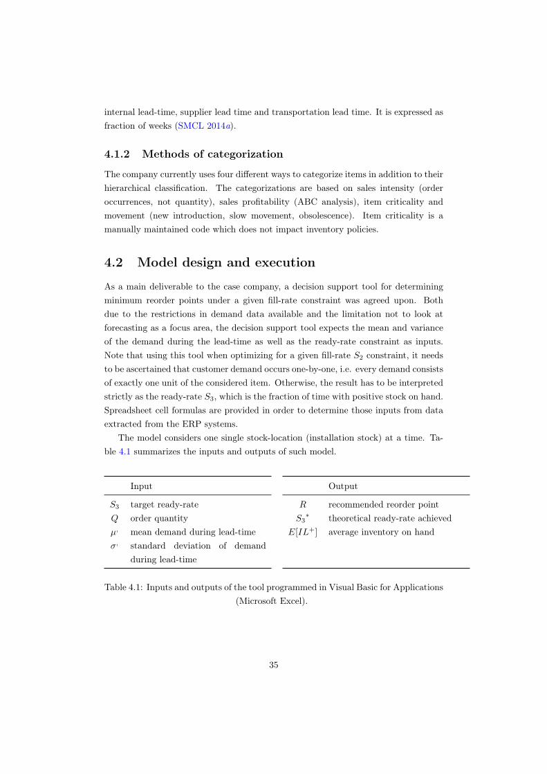
internal lead-time, supplier lead time and transportation lead time. It is expressed asfraction of weeks (SMCL 2014a).

4.1.2 Methods of categorization

The company currently uses four different ways to categorize items in addition to theirhierarchical classification. The categorizations are based on sales intensity (orderoccurrences, not quantity), sales profitability (ABC analysis), item criticality andmovement (new introduction, slow movement, obsolescence). Item criticality is amanually maintained code which does not impact inventory policies.

4.2 Model design and execution

As a main deliverable to the case company, a decision support tool for determiningminimum reorder points under a given fill-rate constraint was agreed upon. Bothdue to the restrictions in demand data available and the limitation not to look atforecasting as a focus area, the decision support tool expects the mean and varianceof the demand during the lead-time as well as the ready-rate constraint as inputs.Note that using this tool when optimizing for a given fill-rate S2 constraint, it needsto be ascertained that customer demand occurs one-by-one, i.e. every demand consistsof exactly one unit of the considered item. Otherwise, the result has to be interpretedstrictly as the ready-rate S3, which is the fraction of time with positive stock on hand.Spreadsheet cell formulas are provided in order to determine those inputs from dataextracted from the ERP systems.

The model considers one single stock-location (installation stock) at a time. Ta-ble 4.1 summarizes the inputs and outputs of such model.

Input Output

S3 target ready-rate R recommended reorder pointQ order quantity S3

∗ theoretical ready-rate achievedµ, mean demand during lead-time E[IL+] average inventory on handσ, standard deviation of demand

during lead-time

Table 4.1: Inputs and outputs of the tool programmed in Visual Basic for Applications(Microsoft Excel).

35

determineinventory level

probabilities for R = -Q

read inputs

determineprobability for

demand k,start with k= 0

add to cumulated demand probabilities

no

yes

FALSE:Poisson

TRUE:NegBin

increase R

determine newprobability value

for inventory level

add value to cumul.probabilities

no

for IL, determineIL x P(IL) and add it

to sum EIL+

increase IL by 1

IL = 0

write outputs

initialize

PS

μ ,   σ ,   Q  S ∗

3

VMR ≥ 1.1

PS ≥ 0.99...

determine reorder point

yes

S3 ≥ S∗

3

evaluate

no

R  E[IL + ]  S3

yes

IL = R + Q

Figure 4.1: Algorithm used in Analysis.

As mentioned in Section 3.12, inventory level probabilities can be re-used leverag-ing a simple conversion of the argument. In the proposed algorithm, the difference ofR and −Q is called addedR. This simplifies looking up inventory level probabilities,as it describes the offset of the inventory level probability array index and j, whichsimplifies using the relationship in (3.22). To enable re-using intermediate results,these are saved in global arrays.

The average stock on hand E[IL+] can then be calculated using (3.24), which isdone once the reorder point has been determined. With this, it is possible to determine

36

min E[IL+] with S2 ≥ S2goal, the algorithm has been visualized in Figure 4.1.A visualization application is also developed and delivered to the company. The

visualization application contains all the results from the decision support tool alongwith other data. Other data included: item costs, recorded inventory levels and itemdescriptions. Therefore, the visualization application is used to quickly filter-out itemsand results which allows for better comparisons. An application overview is presentedin the Appendix.

4.3 Data collection

Quantitative data was collected from different systems. The company uses an ERPsoftware, the database of which can be accessed through a visual query-based interfaceacross different countries. Furthermore, aggregated data from different data sources isavailable through designed-for-purpose applications in a business intelligence software.Throughout the collection process, data was constantly filtered down to match thestudied set of items.

4.3.1 Demand

According to Axsäter (2006), in practice, if a demand is not met it often results ina lost sale and is not recorded. Therefore, it is difficult to measure the real demandunless having high service levels where very few lost sales occur.As per the current distribution network in the case company, there are two maindemand types being recorded:

1. Replenishment orders: internal demand within the downstream organizationand the intermediate organization.

2. Sales orders: end customer orders within the downstream organization and thecustomer (also known as invoiced sales).

Axsäter also mentions the systematic error one often needs to accept when usingsales data instead of real demand data. When the fill-rate is high, it can be assumedthat sales ≈ demand, but if this is not the case, it is complicated to estimate thedemand. If customers ask for an item that is not in stock, this is not necessarilyrecorded in the company’s sales system.Each sales entity in Sandvik has data recorded in an enterprise resource planningsoftware (ERP) which can be accessed separately through a visual form-based queryinterface for each entity. Another software system is being used to compile demanddata into a central platform (business intelligence software).As the proposed model suggests that inventory should be kept in a single centralized

37

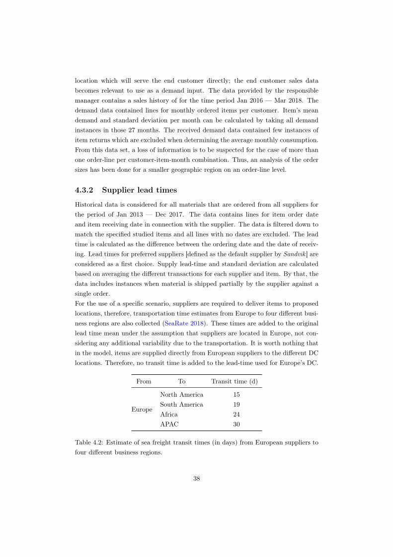
location which will serve the end customer directly; the end customer sales databecomes relevant to use as a demand input. The data provided by the responsiblemanager contains a sales history of for the time period Jan 2016 — Mar 2018. Thedemand data contained lines for monthly ordered items per customer. Item’s meandemand and standard deviation per month can be calculated by taking all demandinstances in those 27 months. The received demand data contained few instances ofitem returns which are excluded when determining the average monthly consumption.From this data set, a loss of information is to be suspected for the case of more thanone order-line per customer-item-month combination. Thus, an analysis of the ordersizes has been done for a smaller geographic region on an order-line level.

4.3.2 Supplier lead times

Historical data is considered for all materials that are ordered from all suppliers forthe period of Jan 2013 — Dec 2017. The data contains lines for item order dateand item receiving date in connection with the supplier. The data is filtered down tomatch the specified studied items and all lines with no dates are excluded. The leadtime is calculated as the difference between the ordering date and the date of receiv-ing. Lead times for preferred suppliers [defined as the default supplier by Sandvik ] areconsidered as a first choice. Supply lead-time and standard deviation are calculatedbased on averaging the different transactions for each supplier and item. By that, thedata includes instances when material is shipped partially by the supplier against asingle order.For the use of a specific scenario, suppliers are required to deliver items to proposedlocations, therefore, transportation time estimates from Europe to four different busi-ness regions are also collected (SeaRate 2018). These times are added to the originallead time mean under the assumption that suppliers are located in Europe, not con-sidering any additional variability due to the transportation. It is worth nothing thatin the model, items are supplied directly from European suppliers to the different DClocations. Therefore, no transit time is added to the lead-time used for Europe’s DC.

From To Transit time (d)

Europe

North America 15South America 19Africa 24APAC 30

Table 4.2: Estimate of sea freight transit times (in days) from European suppliers tofour different business regions.

38

4.3.3 Crusher components list and crushers’ demand

The parts in focus are also used to produce new machinery [new equipment], therefore,some parts demand is present for production purposes. The production entity for newequipment at the case company uses different item codes and places orders with thesuppliers independently. In order to be able to include this demand in the analysis,a component list per machine type is required. The list acts as a map to connectitem codes to new equipment. A new demand compilation therefore includes themachine demand along with the after-market demand. In order to create the list, asubject matter expert is consulted and provided with the items in focus in order to beconnected with the machine types. Crusher demand was provided by the company forthe last nine years. However, demand was considered for the period between 2016 —2017. This period showed a stable pattern (no trend and little variability) and wasalso advised by the principal company. Historical new equipment demand per monthhas been been converted to parts demand using the crusher to parts list. This demandhas been merged together with the after-market demand (from Section 4.3.1) to forma new demand mean and standard deviation.

4.3.4 Inventory and stocks on hand

Inventory data is available through the business intelligence software which allowedfor data extraction for a past year. Thus, inventory data for the period of Feb 2017 —Mar 2018 was collected. The inventory is collected on a stockroom level, which thenis aggregated in two ways:

1. Global inventory levels: All data points are aggregated on a monthly level.

2. Regional inventory levels: All data points are aggregated on a monthly level into5 different business regions (North America, South America, Europe / MiddleEast, Africa and APAC)

4.3.5 Service measure: Fill-rate

The principal company records order fulfillment and the status of each order if itwas filled directly from stock or not. The data can be retrieved from the businessintelligence software. The fulfillment status for each customer order line was extractedfor the period of Mar 2017 — Apr 2018. The data show each order-line and whetherif it was fulfilled directly from stock or not. The data was used to create an averagefill-rate for each item. Therefore, it is worth mentioning that the used fill-rate data donot represent the performance of the downstream organization, rather, it representsthe fill-rate performance as perceived by the end customer for the set of studied itemsonly.

39

4.3.6 Lost demand

A semi-structured interview was carried out with a sales manager in Northern Eu-rope. Because of the poor quantitative data quality (assessed together with companyrepresentatives) a further quantitative analysis was not pursued. The quantitativedata included information on quotations, the geographical spread of crushers soldand crushers known as active. The interview is the main data input to investigatelost sales. This is further described in Chapter 6.

40

Chapter 5

Analysis

This chapter is intended to deliver and explain the findings of the thesis in detail. Asthe results of the mathematical model include a large number of items, main findingsare presented in groups and a selection of items that represent a group of findingsis taken to a more detailed level of analysis. Furthermore, this chapter discussesadvantages and disadvantages of centralizing after-market spare parts inventory.

5.1 Different scenarios

The initial model (Scenario 1) considers the case company’s current distribution net-work a black box. Distribution from the suggested DC to customers currently includestockrooms that are managed by the respective downstream organization. This fullycentralized solution is a very idealized model. A comparison of this first model withreality in a step of validation has resulted in the decision of considering a secondmodel that comes closer to the reality (Scenario 2). This adjusted model considersthat the customer does not experience shelf availability but rather a waiting time untilorder fulfillment. In this regards, decentralization of inventory would be consideredas positive by the customer. At the same time, a centralized solution offers the casecompany better control of their inventory. This is due to reducing the safety stocksas demand uncertainty is diminished. However, a centralized solution would requireexpress shipments of parts to customers who are potentially facing a business inter-ruption. To add more complexity, the studied items can mostly be described as largeand heavy items which might create additional barriers for express shipping. Thus,Scenario 2 includes five different distribution centres based on the business region.This scenario is thought to provide a middle ground for the mentioned dilemma.

41

Currently, the inventory management for the production organization at the casecompany is relatively independent from the inventory management of spare parts.The studied items are required by both; the after-market and the production of newequipment. Therefore, same parts can be ordered, stored and replenished separately.While the software systems are not fully aligned to accommodate a high visibilityof similar items used in production and after-market, it was in the management’sambitions to consider both types of demands in the inventory model. Thus, a scenariothat includes both types of demands is introduced (Scenario 1P).

From the historical data the conclusion is that order sizes equal to 1 in most cases.Therefore, it is worth noting that for the numerical results in this thesis, the orderquantity is assumed to be Q = 1, however the decision support tool is designed forvariable values of Q. Please see Section 4.2 for a detailed explanation of the decisionsupport tool. A detailed description for the mentioned scenarios will be provided inthe following sections.

5.1.1 Scenario 1: Fully centralized after-market demand

The first model looks at the upper bound for inventory level reductions due to cen-tralization efforts by merging all demands on a global level and serving them by directdeliveries from a single warehouse. Therefore, achieving the least variability in thesystem (see Figure 1.4).

For this model, the main stochastic inputs that are used:

1. Sales consumption (invoiced): After-market collected sales averages (see Section4.3.1) are represented by two statistical measures for each studied item (µd andσd).

2. Supply lead times: Collected lead times of supplies (see Section 4.3.2) are alsorepresented by the statistical measures (µLT and σLT ) for each item.

Both data inputs are subject to a data cleaning process (see Section 4.3) mainlyby filtering and excluding data with missing order lines. Both inputs are compiledtogether following (3.6) and (3.7) forming µ, and σ,, respectively. Entering theseinputs, along with the targeted service level (fill-rate = 95%), into the decision supporttool returns the following inventory parameters:

1. Re-order point

2. Achieved service level (fill-rate)

3. Expected inventory level

Furthermore, Figure 5.1 visualizes the steps for this model.

42

Global demand for AM parts Supply lead-timesDesired service level

Inputs

1. Re-order points2. Achieved service level3. Expected inventory levels

Output

DataCleaning

Run thedecision

support tool

Process

CompilingDemand and

Supply lead-timedata

Figure 5.1: Data modeling for Scenario 1

5.1.2 Scenario 2: Partially centralized after-market

A more realistic scenario that considers the customer’s willingness to wait and con-siders the fact that items are very heavy (and costly to ship by air), has been set upby modelling one inventory location per geographic business area. For this scenariothe same sales data is used as in Scenario 1 (Section 5.1.1) but now divided into fivemodels; Europe and Middle East, Africa, North America, South America and APAC.Figure 5.2 shows these inventory locations in different business regions (5.2a) alongwith the distribution network (5.2b) for this scenario. Scenario 2 assumes that the fiveregional DCs are independent from each other and that each DC represents a singleechelon optimization problem with infinite supply and variability in supply lead-time.

NorthAmerica

South America

Europe & ME

Africa

APAC

(a) Scenario 2 geographical DCs spread

Suppliers

Production -Svedala 

Europe EndCustomers

Europe & ME

Africa

SA

NA

APAC

Africa EndCustomers

APAC EndCustomers

SA EndCustomers

NA EndCustomers

(b) Scenario 2 distribution network

Figure 5.2: Scenario 2 distribution network

The suppliers data base for the case company showed that the vast majority ofall suppliers of the studied items are based in Europe. Therefore, it was assumed forthis scenario that items to be shipped to other locations than Europe will experiencea delay caused by shipping the items using sea freight (see Table 4.2). Uncertaintyrelated to transit times was not taken into consideration. Thus, the supply lead timeconsidered differs based on storage location. Combining demand, supply lead-timesand transit times produced the statistical measures µ, and σ,. Figure 5.3 shows thesteps for modeling Scenario 2.

43

1. Five different regional DC's2. Regional demand for AM parts3. Supply lead-times4. Transit times to locations5. Desired service level

Inputs

For each regional DC

1. Re-order points2. Achieved service level3. Expected inventory levels

Output

DataCleaning

Run thedecision

support tool

Per Region

Process

CompilingDemand AM andSupply lead-time

data  Per Region

Figure 5.3: Data modeling for Scenario 2

5.1.3 Scenario 1P: Centralized after-market and productiondemand

It was hypothesized whether a combination of after-market demand and the demandfor parts in new equipment production would help in setting up a combined inven-tory system. This would allow to reduce new equipment production lead-times (seeFigure 5.4).

Supplier

Production - Svedala 

> 95 %S2

Global Warehouse

Production - Svedala 

N EndCustomers

Figure 5.4: Distribution network featuring a high fill-rate global warehouse for partsthat can be used as after-market spare parts or in new equipment production.

For this scenario, the model is similar to the model in Scenario 1, but, with ademand aggregation to include the following two types:

1. Sales consumption (invoiced), as in Scenario 1 (see Section 5.1.1)

2. Combination of crushing equipment sub-assembly information and equipmentsales into new production parts requirements as described in Section 4.3.3.

Both demands were compiled in a single data set and the statistical measuresµd and σd were calculated. Then, the scenario followed the same procedure as in

44

Scenario 1 by combining the stochastic lead times of supplies to finally end up withµ, and σ,. Figure 5.5 shows the steps for modeling Scenario 1P.

1. Global demand for AM parts 2. Global demand for Crushers3. Supply lead-times4. Desired service level

Inputs

1. Re-order points2. Achieved service level3. Expected inventory levels

Output

DataCleaning

Run thedecision

support tool

Process

CompilingDemand (AM &Crushers) and

Supply lead-timedata

Figure 5.5: Data modeling for Scenario 1P

45

5.2 Identifying demand patterns

In order to provide an overview of the different types of demand, the four-field matrixintroduced in Section 3.2 is used to categorize the sample into the classes of inter-mittent, lumpy, smooth and erratic demand. Examples of demand time series for thefour different categories can be seen in Figure 5.6.

smootherratic

intermittentlumpy

0

5

10

15

20

25

0 1 2 3 4

Av

era

ge

De

ma

nd

In

terv

al A

DI

Coefficient of Variation of Non-Zero Demands CV²

(a) overview of example items

(b) intermittent demand (c) lumpy demand

(d) smooth demand (e) erratic demand

Figure 5.6: Demand graphs over time of example items.

46

0

5

10

15

20

25

0 1 2 3 4

(a) all items

0

1

2

3

4

5

6

7

8

9

10

0 0,2 0,4 0,6 0,8

(b) detail view

Figure 5.7: Investigated items in the four-field matrix by Syntetos et al. (2005): vari-ability of non-zero demand periods CV 2 on horizontal axes, average demand intervalADI on vertical axes.

Figure 5.7 gives an overview of the result of our investigation using the four-fieldmatrix suggested by (Syntetos et al. 2005). The considered item population splits upin the four categories as shown in Table 5.1. Note the difference in fill-rate S2 actual

for smooth demand items, which indicates that current methods work better withsmooth demand patterns.

Table 5.1: Overview of items in demand categories

# of items share S2 actual

intermittent 90 55 % 36.6 %

smooth 56 34 % 65.4 %

erratic 9 6 % 43.5 %

lumpy 8 5 % 32.6 %

The analysis has been carried out on a global demand level, i.e. on the highestpossible level of aggregation. The review period used in the analysis is one month andthere has been no advanced forecasting applied, instead the whole population of 26

months is used with equal weighting for all periods in determining ADI and CV 2. Ofthe investigated item sample, 35 items are demanded every month, i.e. ADI = 1. 13

items only have one recorded demand during the period investigated, which results invery high levels of ADI (depending on the time instance of the recorded demand, asonly non-demand periods that occurred before a recorded demand are considered).

Table 5.2 illustrates the relationship of the popularity of a machine type (column)and their corresponding spare parts’ demand by component type (row). The four

47

Table 5.2: Overview of machine types and their respective spare-parts’ demand pat-tern, abbreviated by their initials: Smooth, Erratic, Intermittent, Lumpy.

MT1 MT2 MT3 MT4 MT5 MT6 MT7

sale .18 .21 .21 .06 .05 .06 .03fleet .13 .28 .27 .02 .03 .06 .02

Major I I I I I I IMajor S S I I I I IMajor S I I I I I IKey S S S E I L IKey S L E I L I IKey S S S S E I IKey E S I I I I IKey S E S S S I –Key I I I I – I IKey S S S S S I IKey S S – E – S –Key S S S S S S SKey S S S S S S IKey S S S S S S SKey S S S S S I S

demand types introduced in Section 3.2 are abbreviated with their initials. It isinteresting to highlight that especially the very popular machine types MT1 andMT2 generate a lot of smooth demand patterns on a global level. Furthermore,the different component types (rows) generate different kinds of demand patternsacross the machine types (columns): The very large, heavy and expensive majorcomponents in rows 1–3 most often exhibit a rather intermittent demand, while somekey components generate a rather smooth demand pattern across machine types (lastfour rows).

48

5.3 Expected inventory levels E[IL+]

The inventory optimization (see Section 4.2) resulted into providing two main param-eters: the reorder point R and the expected inventory level E[IL+]. While the reorderpoint R is the controllable measure that the company can further implement in orderto apply the inventory policy, the expected inventory level E[IL+] is considered asthe key measure for analysis. E[IL+] acts as a comparable measure for the currentsituation at the case company.

Actual inventory levels (ILactual) and actual fill-rate (S2 actual) are representativesfor the current performance of the case company. Data collection for these measuresis explained in the previous chapter (see Sections 4.3.4 and 4.3.5).

Recall that Scenario 1 considers a single after-market inventory location, Sce-nario 1P also includes demand from new equipment production and Scenario 2 looksat five different geographic regions with dedicated stocking location. Each scenarioproduced a number of items that E[IL+] either need to be increased or decreased ifcompared to the current inventory levels (ILactual). An overview for the results ispresented in Figure 5.8. It shows average numbers for the whole sample.

0%

10%

20%

30%

40%

50%

60%

70%

80%

90%

100%

0

0.5

1

1.5

2

Actual Scenario 1 Scenario 2 Scenario 1P

Fill

-ra

te

No

rma

lize

d I

nv

en

tory

lev

el

Inventory level Fill-rate goal Fill-rate

Figure 5.8: Overview of the results for the expected inventory levels (Normalizedinventory levels)

49

Under the current actual inventory system, the case company is not achieving thedesired fill-rate constraint (95%). Generally, all three scenarios increase the averagefill-rate by 55% if compared to current situation. Fully centralizing inventory (Sce-nario 1) will reduce the average E[IL+] by 28 % from current levels, while meetingthe fill-rate constraint at 95%. On the other hand, the partially centralized model(Scenario 2) will increase E[IL+] on average by 40 % if compared to the current ac-tual, however, it will provide much higher fill-rate (55% increase in fill-rate to meetthe constraint at 95%). If Compared to Scenario 1, Scenario 2 is expected to doublethe E[IL+]. Scenario 2 provides higher availability for customers because items havehigh fill-rate (shelf availability) and generally much shorter transportation times tocustomers compared to Scenario 1.

Adding the production consumption to Scenario 1 will result into a 50 % increase inE[IL+] while meeting the fill-rate constraint at 95%. Moreover, this increase is a resultmainly driven by the major components. The major components are currently madeto order, therefore, a significant increase in E[IL+] is reasonable when considering anR,Q policy instead.

More specific analysis is conducted. The items are further analyzed regardingtheir inventory performance in different scenarios. Each item belongs to an "increase"group or a "decrease" group. However, for some items the relative inventory difference(∆) is small (±10 %), and thus, worth analyzing separately. Table 5.3 illustrates thenumber of items found in each scenario and categorizes them into the three definedgroups. Items that did not have any demand over the course of the collected period(see Section 4.3.1) or did not have any supply lead time data (see Section 4.3.2)resulted into not including the item in the study. Therefore, Table 5.3 also shows thenumber items with missing data.

Table 5.3: High-level comparison of actual inventory levels

increase∆ > 10%

decrease∆ < −10 %

∼ same−10 % < ∆ < 10 %

missing data

Scenario 1 49 100 16 41Scenario 2 106 32 27 41Scenario 1P 86 67 25 28

In order to examine all cases ("increase", "decrease" and "same") shown in Ta-ble 5.3, a selection of items that represent these cases are taken into further analysis,these items are shown in Table 5.4. Item A represents an inventory increase acrossall scenarios. Item B represents an inventory decrease across all scenarios. Item Crepresents a roughly similar inventory performance required for Scenario 1 and 1P,

50

and finally, Item D represents a roughly similar inventory performance required forScenario 2. Scenarios 1 and 1P can be considered equal for the upcoming analysisand will be differentiated by the end of this section.

Table 5.4: Item group representatives

increase decrease ∼ same

Scenario 1Item A Item B

Item CScenario 2 Item D

5.3.1 Category “increase”

Item A represents the set of items that have a lower current inventory level than whatthe model suggests to achieve (the desired fill-rate S2). Figure 5.9a shows the expectedinventory level E[IL+] and the fill-rate S2 for all scenarios versus the ILactual andS2 actual. Scenario 1 and 1P suggest increasing the inventory to achieve a 95 % fill-rate.This shows two main effects:

1. The effect of increasing inventory in order to meet the demand and thus achievea higher fill-rate.

2. The effect of centralizing inventory; by keeping lower safety stocks in a fully cen-tralized network (Scenario 1 or 1P) versus a less centralized network (Scenario 2)where the amount of required safety stock is higher to cover more uncertainty.

Globally, an item might have an adequate amount of stocks but in a location thatis different than where the demand occurs. This results in missing customer orderlines and obtaining a lower service level. This can be shown by comparing the actualinventory development over time on a regional level with the global inventory level(Figures 5.9c and 5.9b, respectively). It is worth noting that both levels consist ofthe same inventory records from all stockrooms but are aggregated on two differentlevels. In these figures, the global inventory pattern shows no stock-out cases for ItemA, however, the recorded fill-rate is approximately 40 % (Figure 5.9a). A closer lookinto the regional level shows that the item has stock-out instances in Africa, Europeand South America, explaining the low fill-rate. This specific finding is applicableacross all categories and not only here.

5.3.2 Category “decrease”

On the other hand, Item B represents the case of having a high amount of inventory(ILactual) which exceeds the suggested levels of all scenarios (Figure 5.10a). Despite

51

0%

10%

20%

30%

40%

50%

60%

70%

80%

90%

100%

Actual Scenario 1 Scenario 2 Scenario 1P

Fill

-ra

te

Inv

en

tory

lev

el

Inventory level Fill-rate goal Fill-rate

(a) IL+ & S2 performance

Inv

en

tory

lev

el

Africa APAC Europe North America South America

(b) ILactual development on a regional level

(c) ILactual development on a global level

Figure 5.9: Item A: category increase

having high amount of inventory, item B still doesn’t satisfy the 95% fill-rate target.For this particular item the current fill-rate is approximately 90 %. All modeledscenarios suggest lower inventory levels to achieve the desired fill-rate. Similar toItem A, the centralization effect is present (lower inventory levels satisfy a higherfill-rate) as the actual case fill-rate is relying on having the item in stock at thestock room level (including country level). Even if no stock-outs are present on theregional level (Figure 5.10b), an order line can be missed on a country stockroomlevel therefore having a 90 % fill-rate instead of a 100 %. It is also worth notingthat in this category items with very low fill-rates (lower than Item B) are observedand the same justification is applicable, as having the stocks in the wrong locationwill result in having high inventory levels and low fill-rates. This group can also beidentified as the group of items that has the potential of lowering tied up capital, aslower inventory levels would suffice to achieve better fill-rates compared to the actualsituation.

One can argue that Scenario 1 (or 1P) fill-rate is comparable to Scenario 2 onlyif the difference in transportation time is considered. Customers experience a longertransportation time in a highly centralized distribution network (Scenario 1) whencompared to a less centralized network (Scenario 2). Thus, the waiting time experi-

52

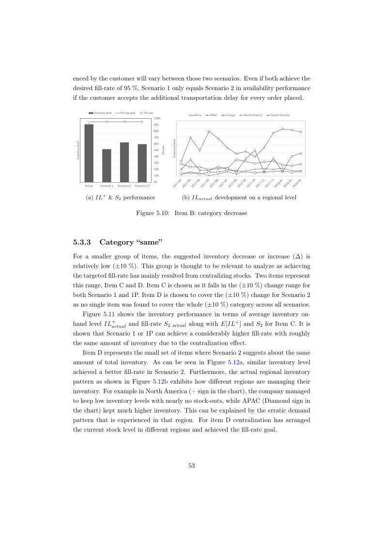
enced by the customer will vary between those two scenarios. Even if both achieve thedesired fill-rate of 95 %, Scenario 1 only equals Scenario 2 in availability performanceif the customer accepts the additional transportation delay for every order placed.

0%

10%

20%

30%

40%

50%

60%

70%

80%

90%

100%

Actual Scenario 1 Scenario 2 Scenario 1P

Fill

-ra

te

Inv

en

tory

lev

el

Inventory level Fill-rate goal Fill-rate

(a) IL+ & S2 performance

Inv

en

tory

lev

el

Africa APAC Europe North America South America

(b) ILactual development on a regional level

Figure 5.10: Item B: category decrease

5.3.3 Category “same”

For a smaller group of items, the suggested inventory decrease or increase (∆) isrelatively low (±10 %). This group is thought to be relevant to analyze as achievingthe targeted fill-rate has mainly resulted from centralizing stocks. Two items representthis range, Item C and D. Item C is chosen as it falls in the (±10 %) change range forboth Scenario 1 and 1P. Item D is chosen to cover the (±10 %) change for Scenario 2as no single item was found to cover the whole (±10 %) category across all scenarios.

Figure 5.11 shows the inventory performance in terms of average inventory on-hand level IL+

actual and fill-rate S2 actual along with E[IL+] and S2 for Item C. It isshown that Scenario 1 or 1P can achieve a considerably higher fill-rate with roughlythe same amount of inventory due to the centralization effect.

Item D represents the small set of items where Scenario 2 suggests about the sameamount of total inventory. As can be seen in Figure 5.12a, similar inventory levelachieved a better fill-rate in Scenario 2. Furthermore, the actual regional inventorypattern as shown in Figure 5.12b exhibits how different regions are managing theirinventory. For example in North America (+ sign in the chart), the company managedto keep low inventory levels with nearly no stock-outs, while APAC (Diamond sign inthe chart) kept much higher inventory. This can be explained by the erratic demandpattern that is experienced in that region. For item D centralization has arrangedthe current stock level in different regions and achieved the fill-rate goal.

53

0%

10%

20%

30%

40%

50%

60%

70%

80%

90%

100%

Actual Scenario 1

Fill

-ra

te

Inv

en

tory

lev

el

Inventory level Fill-rate goal Fill-rate

Figure 5.11: Item C: ∆ = ±10 % for Scenario 1 and Scenario 1P

0%

10%

20%

30%

40%

50%

60%

70%

80%

90%

100%

Actual Scenario 2

Fill

-ra

te

Inv

en

tory

lev

el

Inventory level Fill-rate goal Fill-rate

(a) IL+ and S2 performance

Inv

en

tory

lev

el

Africa APAC Europe North America South America

(b) IL+ development on a regional level

Figure 5.12: Item D: ∆ = ±10 % for Scenario 2

5.3.4 Integrating production

Scenario 1P was motivated by case company’s interest in the possibility of utilizingthe high fill-rate DC for production as well. This model would prove to be beneficialif the production consumption does not form a high disturbance in variability. Theeffect on the expected inventory level depends on the correlation between the twodemand types. An initial evaluation based on the relative change in the value-to-mean ratio of all items reveals that the inventory system would experience mostlysmall changes in this regard. In total, 174 of the items under investigation wereconsidered in Scenario 1P. 50 % of these items exhibit a relative change of ±10 % inVMR. 21 % of the items show a more significant relative decrease, while another 21 %

show a more significant relative increase of up to 60 %.However, when looking at the resulting average inventory on-hand, the comparison

of Scenario 1 and Scenario 1P shows significant increases in expected level of inventoryon-hand resulting from the optimization under the fill-rate constraint of 95 %, which is

54

Figure 5.13: Overview of change in on-hand inventory level when integrating produc-tion demands with the fully centralized aftermarket inventory.

illustrated in Figure 5.13: While 25 % of the items only exhibit an on-hand inventoryincrease of 30 % or less compared to Scenario 1, 11 % of the items in Scenario 1Pexhibit an expected inventory level that is more than three times as high as theirresult in Scenario 1. A general benefit from merging the two demand types can thusnot be deduced.

5.3.5 Summary of scenario analysis

Currently, the inventory system of the / is highly decentralized across their geo-graphical markets. One option to increase the efficiency of inventory managementis centralization. But as motivated earlier, Scenario 2 resembles the most feasiblesolution for the case company. Logistics costs for this type of spare parts are veryhigh if one warehouse needs to cover the entire global demand. Spare parts are oftenordered with urgency (i.e. as a result from machine stoppage), thus, need to be de-livered within an acceptable time frame. In addition, some parts are not applicablefor express shipping. For example it is almost impossible to ship a major componentusing air freight because of it’s weight and shape. Having five warehouses across theworld could act as a variability buffer for the upstream supply chain, while at thesame time, increase speed of delivery to the end customer.

55

Scenario 2 can be further analyzed by conducting a two-way categorization interms of demand pattern and expected inventory levels. Table 5.5 shows the breakupof items in Scenario 2 with the corresponding demand pattern (see Section 5.2). Itis worth mentioning that some items with missing data from both sides (demandpattern or inventory level analysis) could not be reflected in this table.

Table 5.5: demand shape vs performance (actual versus Scenario 2)

increase decrease same S2 actual

intermittent 64 12 12 36.6 %smooth 27 17 12 65.4 %erratic 5 3 1 43.5 %lumpy 6 1 1 32.6 %

As can be seen in Table 5.5, the largest number of items that need for inventoryincrease belong to the intermittent demand (64 items). Furthermore, looking at thecurrent fill-rates (S2 actual) recorded for items with intermittent demand, it is as lowas 36 %. The low fill-rate explains the need of inventory increase in Scenario 2. Also,intermittent demand is difficult to manage and can explain the current low fill-ratefulfillment by the case company. On the other hand, smooth demand is relativelyeasy to manage and therefore achieves a better fill-rate (65 %). However, 27 itemsstill need an inventory increase to achieve the desired fill-rate. This relationship (anincrease in on-hand inventory is required to increase the fill-rate) is expected.

It is also worth noting that the low fill-rate numbers (shown in Table 5.5) mightshow critical business situation for the case company. Low spare parts order fulfillmentcan create significant issues for customers. However, the case company still provideits customers with the spare parts from a nearby location even if the demand was notmet from the first instance. So these fill-rates do not directly represent the servicelevel that the customer is experiencing.

5.4 Centralization: Factors and Performance

Performance regarding inventory centralization and decentralization will be furtherdiscussed. Certain attributes are important to analyze in order to get a better holisticunderstanding of the model. These attributes are formulated in Table 5.6. The tableis based on the literature that can be found in Table 3.1, however, not all attributesare discussed as this thesis focuses on inventory management.

Waiting times for customers are often higher in a centralized solution as the ware-house is located further away if compared to a decentralized solution. The only

56

Table 5.6: Overview of implications of centralization decisions.

Attribute Centralized Decentralized

PerformanceTarget

Customerwaiting time

Generally longer, but onlydue to transportation

shorter when item available

Inventorylevel at thesame S2

Lower Higher

Time ininventory

Lower Higher

Networkstructure

Number ofDCs needed

Lower Higher

PlanningProcess

Demandvariability

Lower, as individual andregional demand patternsmerge into one global de-mand pattern that is easierto forecast

Higher, as the demand isforecasted on a lower levelof aggregation

Supplyvariability

Controlled by bufferingstocks in a single location

Less controllable, assmaller demand is orderedfrom suppliers

difference between those two solutions is believed to be the delivery delay caused bythe transportation time to the customer.

As shown in Section 5.3, expected inventory levels in a fully centralized solution islower than in a partially centralized solution for the same targeted fill-rate (Scenario 1and 2, respectively). All under the assumption that demand is independent.

The inventory performance measure (inventory turnover) can help in determiningthe expected number of replenishments needed. Companies can not store materialsfor very long period of time as the held materials need to be converted into sales inorder to have a healthy cash flow. Furthermore, inventory turnover measure is oftenexpressed in terms of average days needed for a stocked item to be converted intosales (Days of Supply DOS, see Section 3.7). DOS for Scenario 1 is estimated to be65 days, while in Scenario 2 the average DOS for all regions is 92 days. A higherDOS indicates that the inventory is kept for a longer time and thus tying up capitalfor longer periods.

Section 3.13 introduced the “square root law”, the percent reduction when cen-

57

0

20

40

60

80

< 0 = 0 [0,.125)

[0.125,0.25)

[0.25,0.375)

[0.375,0.5)

[0.5,0.625)

[0.625,0.75)

[0.75,0.875)

freq

uenc

y (n

o. o

f ite

ms)

relative reduction of on-hand inventory

Figure 5.14: Reduction in on-hand inventory histogram

tralizing inventory given certain assumptions. It is interesting to highlight that incontrast to the simplifying expectation of the percent reduction from five inventorylocations to one (Scenario 2 versus Scenario 1) being 1 − 1√

5≈ 55 %, the numerical

modeling shows that for the items under investigation, the average per cent reductionis rather about 38 %. However, for a large group of items, the change in on-hand in-ventory when changing from five inventory locations to one inventory location is about50− 62.5 %, which is in line with the claim made by the aforementioned “square rootlaw” (see Figure 5.14).

5.4.1 Determining item centralization level

The question of whether to centralize the after-market distribution network for thecase company can not be answered on a global level using the results from the ana-lyzed model. It is necessary to consider additional information and thus, the analysisis providing a support tool for such a decision. Among the factors to consider arethe end-customer location, resulting transportation time to the customer, their in-stalled base and promises towards them. An item-by-item procedure is suggested.In which, the demand patterns along with actual and optimized data are considered

58

both globally and on a regional basis. This process can be done using the deliveredvisualization application (Appendix page 74).

Scenario 2 considers five geographic regions. It is suggested (on an item level) tocompare these regions, and determine whether there are any outliers with regards tothe inventory level suggested (for example in days of supply DOS) and the demandtype identified (the demand variability per period with demand CV 2 and the averagedemand interval ADI). Regions that exhibit relatively smooth demand patterns couldbe allowed to continue keeping stocks in a regional inventory, while regions with moredifficult demand patterns can be considered for centralization. In the same way itemswith a significant difference in expected inventory on hand in Scenario 1 and Scenario 2can be considered for centralization.

59

Chapter 6

Discussion about the impact oflost sales

The research question “How can lost sales be related to the suspected availability is-sues?” has not been taken up in the Chapter 5 due to a lack of reliable data. Thepreliminary findings and possible further actions are thus discussed in this chapter.

6.1 Approaches

Different kinds of data were gathered in order to shed light on the questions (1)whether there have been lost sales, (2) what the reasons for the phenomenon are,and (3) how the impact on demand patterns and thus expected inventory levels canbe quantified. Information relevant to those questions that have been collected aspart of the main study are after-market parts demand information (see Section 4.3.1)and the crusher-to-parts relationships (see Section 4.3.3). In order to investigate theabove questions, data has been collected regarding quotations, the equipment fleetand customer decision making.

In order to answer the question of the general existence of such a problem, after-market sales can be compared to quotation data for after-market parts. Quotationdata is compared to order lines using an analysis tool of the ERP used at the company.An initial analysis of the data record shows that reasons not to order based on aquotation are often either not known or not recorded in the system, which is why thisdata is not further considered. Furthermore, customer requests that do not turn intoquotations are not available for analysis as the data is not recorded in this specificsystem.

60

Alternatively, sales of spare-parts per group of crushers (either on a region, coun-try, customer or site level) can be considered relative to the number of crushers. Asthe equipment sales history does not necessarily represent the active machine popula-tion, such a list of active equipment was acquired from the company. Sales managersof the respective geographic regions are responsible for the data management. Thebusiness intelligence tool is still in the process of being built during the time of thestudy.

Thus, a preliminary data set was used as a preview of what kind of analysis willbe possible in the future. Initial data analysis regarding sold crushers and activemachine population leads to suspicions of discrepancy between machine populationand sales of after-market spare parts. Some countries show much stronger after-market sales when compared to others. For example, two countries can have a similarmachine population (both in terms of sales and recorded active crushers) but have acompelling gap in after-market sales.

Due to the general lack of reliable information for an approximation of the magni-tude of lost sales, the question for an adjustment of the demand forecast or inventorylevels for lost sales can not be answered properly.

6.2 Lost sales and inventory centralization

A semi-structured interview with a sales manager was carried out in order to geta better understanding of the underlying factors of lost sales at the case company(Carlqvist 2018). The collected information focuses on exploring factors affecting lostsales and the relationships it induces.

Parts failures at customer sites depend on unpredictable factors such as machineutilization, machine setup, rock type, maintenance procedures and many more. There-fore, a qualitative understanding of the end customer perspective for spare parts pur-chasing is to be analyzed here.

The interviewee deems the market share in Sandvik cone crusher spare parts busi-ness satisfactory regarding their geographic scope of responsibility (Northern Europe).Customers in this region enjoy a high fill-rate due to the proximity to the distributionnetwork. It is explained that endeavours to further increase the market share wouldnot necessarily have a positive impact on the overall company profitability e.g. dueto investments or price reductions (Carlqvist 2018).

The business intelligence tool for comparing after-market sales performance withpotential sales is based on average spare parts consumption as well as proactive main-tenance workshops (Norden & Svennelid 2018). It is yet under development butdeemed a welcome aid for sales work, however doubts are raised regarding the neces-sary data. It is argued that customers behave differently from each others and that

61

even two sites for the same customer may have very different spare part consumptionpatterns (Carlqvist 2018).

During the research, it was hypothesized whether an increased availability couldhave a positive effect on sales. The interviewee highlighted that this might be truefor customer retention, but not regarding the initial after-market buying decision.According to the subject matter expert, the customer assumes that the case companyis able to offer a high availability in line with the premium brand image established(Carlqvist 2018).

However, to observe the relation and quantify it, lost sales should be investigatedmore deeply. This could be done by collecting both more direct and indirect data.Direct data about customers, their crushers and specific parts consumed on a regularbasis would strengthen the ability to analyze the spare parts demand share for aspecific customer. One possibility for the company to collect relevant direct data is touse technologies related to the Internet of Things (IoT) for live data collection, e.g. itwould be possible to let the equipment report its status and the condition of differentparts through the internet to the case company data centers. On the other hand,indirect data could also be helpful, e.g. sales performance and overall market sharefor the purpose of benchmarking. Today, the case company might not be interestedin providing machine up-time as an after-market service (Carlqvist 2018) but whenhaving enough information about how crushers are being operated at customer sites,it might become an attractive opportunity. The business intelligence tool is a startingpoint for collecting this data and might have a major impact on forecasting for after-market parts. The data might be required to be customer and country specific.

It is known that there is a general causality of low availability and lost sales(Axsäter 2006). However, it is not the only reason for lost sales, which makes itdifficult to estimate the volume of sales lost because of a lack of availability. Ac-commodating additional expected demand (that is expected to be gained because ofraising service levels) in the centralized model is considered not to be as challengingas determining the magnitude of the lost sales due to availability. Should more infor-mation on lost sales become available in the future (e.g. due to more insights from thebusiness intelligence tool and other market research endeavours), it can be consideredusing manual forecasting (or an adjustment of the automatic forecast). If there infact is an increase in sales due to an increase in availability, this can be taken care offrom an inventory control point of view by regularly updating the demand forecastand thereby the inventory parameters.

When introducing the idea of express distribution from few inventory stockinglocations to the customer, a note of caution is raised: Transportation of large partswould pose a problem, as air freight is considered impractical from the interviewee’sperspective and road transport might take a considerable amount of time depending

62

on the distance to the end-customer (Carlqvist 2018). Furthermore, the intervieweehighlighted that a static logistics solution would not help solve the lost sales issue.Rather, a solution should be sought that is tailored around customer base character-istics. For the distribution network, examples for relevant characteristics are:

• Sales channel: direct sales or sales through a distributor.

• Customer stock keeping: inventory is kept or not.

• Uptime criticality: mining customers lose valuable production time if a crusheris not operating, while many construction customers have some flexibility withregards to machine uptime.

• Customer’s stance on preventive maintenance, utilization and material proper-ties.

Depending e.g. the above criteria, customers might consider delivery speed as anorder winner or qualifier (see Section 3.1). In combination, these factors define theimpact of inventory keeping on the end-customer. This will help to better estimatethe trade-off magnitude between costs, service levels and inventory turns.

63

Chapter 7

Conclusion

This conclusion chapter reflects back on the main findings for this thesis. The findingsdescribed in the previous chapter are connected and used to answer the researchquestions. Limitations and future research are then highlighted.

It was hypothesized that centralizing inventory should in general lower the amountof safety stock necessary in the distribution network. The case company’s main issueis related to availability. Therefore, it was also expected that an inventory model thattargets a higher fill-rate will increase the amount of inventory kept, disregarding ifthe inventory is centralized or not. The findings in this thesis are aligned with this.The main findings for the modeled scenarios are as follow (based on average numbersfor all studied items):

• Fully centralizing the inventory (Scenario 1) will result into lowering the to-tal inventory by 28 % (on average) if compared to the current situation whileincreasing the fill-rate by 55 %.

• Partially centralizing the inventory (Scenario 2) will increase the total inventoryby 40 % (on average) if compared to the current situation while increasing thefill-rate by 55%.

• Partially centralizing inventory is expected to double the amount of inventory(on average) if compared to the centralized model (Scenario 2 vs Scenario 1)while both are achieving the fill-rate constraint at 95 %. However, Scenario 2has a quicker delivery to the customer if compared to Scenario 1.

• Including the production demand into the fully centralized model (Scenario 1P)will induce an increase of 50 % (on average) for the total inventory if comparedto Scenario 1 to achieve the same fill-rate constrain at 95 %.

64

It is recommended to consider centralization on an item-by-item basis. Scenario 1and Scenario 2 both represent more centralized models if compared to the currentlyused distribution system and thus can only provide an indication of the potential ofcentralization. The delivery speed towards the customer and centralizing inventoryare two conflicting goals. Therefore, an Item-by-item decision to centralize has beenpresented in this thesis. It is recommended to use the provided tools to identify otherpossible combinations of regions and also even less centralized models. In the nextsections, the research questions will be answered in detail.

7.1 How much stock should be kept in a centralized

inventory solution to accommodate a fill rate of

95 %?

The first question aims at providing the case company with numerical values thatthey can use as comparison in current strategic decisions. Furthermore, it generatedinformation that was used to answer the second research question. As highlightedin Section 5.1, three different scenarios were considered: Scenario 1 considers a fullycentralized inventory system serving global after-market demand, Scenario 1P addi-tionally considers new equipment demand and Scenario 2 considers only after-marketdemand served from five different regional DCs.

The current fill-rate for the distributed system that the company follows, doesnot achieve the desired service level (95 %). For many items inventory needs to beincreased in order to meet this constraint.

Scenario 1 and 1P represent an ideal case where the service level is defined asshelf-availability only. However, customers experience service levels differently, as acombination of shelf-availability and delivery speed. Also, for such large and heavyequipment the spare parts can pose a challenge for express shipping due to their phys-ical dimensions. This is especially problematic for the major components due to theirweight and volume. Thus, Scenario 2 was considered to include a more comparablemodel to the current distribution network (see Section 5.1.2). After-market spareparts demand was aggregated on a monthly basis for five regions. Expected inventoryon hand is strictly larger across all items compared to Scenario 1 due to increasinginventory locations. For those items that exhibited the need for increased inventorylevels in Scenario 1, this is accelerated in Scenario 2.

Under the current distribution network, inventory levels have to be increased inorder to achieve the set fill-rate constraint. In more centralized distribution networks,as modeled in this thesis, this has to be done to a lesser extent. For a subset of items,centralization is sufficient to achieve the set fill-rate constraint with the same amount

65

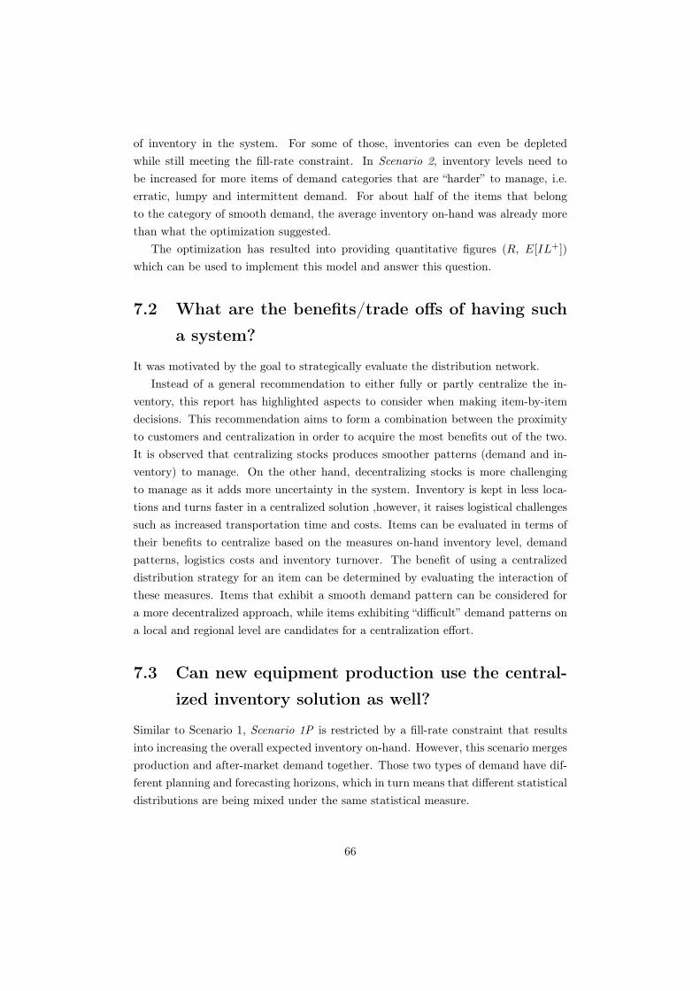
of inventory in the system. For some of those, inventories can even be depletedwhile still meeting the fill-rate constraint. In Scenario 2, inventory levels need tobe increased for more items of demand categories that are “harder” to manage, i.e.erratic, lumpy and intermittent demand. For about half of the items that belongto the category of smooth demand, the average inventory on-hand was already morethan what the optimization suggested.

The optimization has resulted into providing quantitative figures (R, E[IL+])which can be used to implement this model and answer this question.

7.2 What are the benefits/trade offs of having such

a system?

It was motivated by the goal to strategically evaluate the distribution network.Instead of a general recommendation to either fully or partly centralize the in-

ventory, this report has highlighted aspects to consider when making item-by-itemdecisions. This recommendation aims to form a combination between the proximityto customers and centralization in order to acquire the most benefits out of the two.It is observed that centralizing stocks produces smoother patterns (demand and in-ventory) to manage. On the other hand, decentralizing stocks is more challengingto manage as it adds more uncertainty in the system. Inventory is kept in less loca-tions and turns faster in a centralized solution ,however, it raises logistical challengessuch as increased transportation time and costs. Items can be evaluated in terms oftheir benefits to centralize based on the measures on-hand inventory level, demandpatterns, logistics costs and inventory turnover. The benefit of using a centralizeddistribution strategy for an item can be determined by evaluating the interaction ofthese measures. Items that exhibit a smooth demand pattern can be considered fora more decentralized approach, while items exhibiting “difficult” demand patterns ona local and regional level are candidates for a centralization effort.

7.3 Can new equipment production use the central-

ized inventory solution as well?

Similar to Scenario 1, Scenario 1P is restricted by a fill-rate constraint that resultsinto increasing the overall expected inventory on-hand. However, this scenario mergesproduction and after-market demand together. Those two types of demand have dif-ferent planning and forecasting horizons, which in turn means that different statisticaldistributions are being mixed under the same statistical measure.

66

As explored in more detail in Section 5.3.4, Scenario 1P does not exhibit a con-sistent benefit across all items, but for some of the investigated items, the increasein expected inventory levels is relatively low. This makes it possible to consider onan item-by-item basis whether production should be allowed to use this commoninventory in order to shorten the production lead-time for new equipment, as thiscould allow the company to compete on markets with shorter accepted lead-times fornew equipment. However as mentioned before, Scenario 1 and 1P are thought to beidealized models and difficult to achieve practically.

7.4 How can lost sales be related to the suspected

availability issues?

The fourth research question is based mostly on observed discrepancies of the averageconsumption per crusher.

While lost sales and availability are related on a very basic level, in this masterthesis a direct connection could not be formed. Rather, it was discussed that differentfactors can affect lost sales. Further data is needed to form a deep understanding ofthe dilemma. Such data consist of crushers population and working environment foreach customer, reasons behind unsuccessful quotations and spare part criticality tothe customer.

At this stage, it is recommended for the case company to observe demand un-der improved fill-rate performance and continuously update their forecast based ondemand realization.

7.5 Generalizability of the models and research re-

sults

A general and well tested model of single-echelon inventory optimization with a fill-rate constraint has been applied. It is used to evaluate the effects of two differentlevels of centralization of the inventory system, as well as, the integration of produc-tion requirements into the after-market inventory system. The thesis has used thedemand classification by (Syntetos et al. 2005) as relevant criterion to be considered inevaluating the level of centralization of spare parts. No verification of the effectivenessof this categorization for the mentioned purpose has been provided.

The model and its results can be used by the case company to evaluate their currentinventory policies. If conditions change or more accurate information is acquired, themodel can be executed again by the case company using different input values. The

67

model can be easily extended to consider a continuous distribution for smooth, lowvariability demands in order to be more general.

Inventory centralization is a decision that cannot be made relying only on changesin inventory levels but must consider a more holistic view on the entire supply chain.This includes different types of costs (warehousing, transportation, order processing)and effects on performance (fill-rate and customer waiting times).

7.6 Limitations and further research

Limitations of this research were identified earlier in Section 1.5. However, one im-portant limitation for the results is the order quantity when replenishing the DCs.This thesis has assumed continuous review with one-for-one replenishment, howeverwhen using sea freight as suggested in Scenario 2, this type of replenishment mightnot be preferable. With long shipment times, a longer review period or larger reorderquantity are more likely to be employed. Actions like this would lead to an increasedaverage level of inventory on-hand compared to the results of the model presented.

Lead-times used in the inventory control model have been based on the past per-formance of supplier deliveries, both regular and emergency shipments.

The inventory control model used in this thesis treated all demands with a very lowvariance compared to the mean (VMR < 0.9) as if they follow a pure Poisson arrivalprocess; thus the variability might have been slightly overestimated, and therefore,overestimating the necessary average inventory on-hand.

One important part of managing “difficult” demand patterns is forecasting thedemand. This topic has not been treated in the thesis due to the limited scope. Itis however worth looking into a differentiation of the forecasting method based onthe demand categories that have been used in this thesis. Using a good method forforecasting in combination with manual adjustments can help phasing out productsat the end of their product life cycle, thus reducing the risk for obsolete items.

This thesis is part of an end to end logistics study at the case company. Otherstudies regarding the network upstream, specifically supplier lead times and efficientorder quantities are conducted. It is expected that the insights from the supply-sidestudy will be a valuable input to the model introduced in this thesis.

The thesis model assumed direct supplier deliveries to inventory locations. Thisdoes not reflect reality very accurately. In a more advanced model, replenishmentsfrom a central warehouse can be considered.

In order to determine a suitable strategy, the findings from this research couldbe combined with cost assumptions. This would allow for a comparison of differentdistribution scenarios in a total cost analysis.

68

Bibliography

Arnold, J. R. T., Chapman, S. N. & Clive, L. M. (2007), Introduction to MaterialsManagement, number 10, Pearson Prentice Hall, Upper Saddle River, N.J.

Axsäter, S. (2006), Inventory control (International series in operations research &management science), Springer Berlin.

Berling, P. (2008), ‘Holding cost determination: An activity-based cost approach’,International Journal of Production Economics 112(2), 829–840.URL: https://doi.org/10.1016/j.ijpe.2005.10.010

Carlqvist, U. (2018), ‘Personal communication’. Business Line Manager at Crushingand Screening.

Cohen, M. A., Cull, C., Lee, H. L. & Willen, D. (2000), ‘Saturn’s supply-chain innova-tion: High value in after-sales service.’, Sloan Management Review 41(4), 93–101.URL: https://sloanreview.mit.edu/article/saturns-supplychain-innovation-high-value-in-aftersales-service/

Cohen, M. A. & Lee, H. L. (1990), ‘Out of touch with customer needs? spare partsand after sales service.’, Sloan Management Review 31(2), 55–66.

Cook, J. D. (2009), ‘Notes on the negative binomial distribution’.URL: https://www.johndcook.com/negative_binomial.pdf

Dahlborg, C. (2018), ‘Personal communication’. Inventory Management Specialist atCrushing and Screening.

Dahlborg, C. & Ringsbo, J. (2018), ‘Personal communication’. Specialists (InventoryManagement / Project Management) at Crushing and Screening.

Ferrari, E., Pareschi, A., Regattieri, A. & Persona, A. (2006), Statistical Managementand Modeling for Demand of Spare Parts, Springer London, London, pp. 905–929.URL: https://doi.org/10.1007/978-1-84628-288-1_48

69

Fisher, M. (2007), ‘Strengthening the empirical base of operations management’,Man-ufacturing & Service Operations Management 9(4), 368–382.URL: https://doi.org/10.1287/msom.1070.0168

Fleischmann, B. (2016), ‘The impact of the number of parallel warehouses on totalinventory’, OR Spectrum 38(4), 899–920.URL: https://doi.org/10.1007/s00291-016-0442-2

Flynn, B. B., Sakakibara, S., Schroeder, R. G., Bates, K. A. & Flynn, E. J. (1990),‘Empirical research methods in operations management’, Journal of OperationsManagement 9(2), 250–284.URL: https://doi.org/10.1016/0272-6963(90)90098-x

Hill, A. & Hill, T. (2009), Manufacturing Operations Strategy, Palgrave Macmillan,New York, NY, USA.

Hillier, F. S. & Lieberman, G. J. (2001), Introduction to Operations Research, seventhedn, McGraw-Hill, New York, NY, USA.

Hopp, W. J. & Spearman, M. L. (2000), Factory Physics, McGraw Hill.

Israelsson, J. O. (2018), ‘Interview with Supply and Production Planning Manager atSandvik Coromant’. Personal communication.

Kovács, G. & Spens, K. M. (2005), ‘Abductive reasoning in logistics research’, Inter-national Journal of Physical Distribution & Logistics Management 35(2), 132–144.URL: https://doi.org/10.1108/09600030510590318

Kvale, S. (2007), Doing Interviews, SAGE Publications, Ltd.URL: https://doi.org/10.4135/9781849208963

Larsen, C. & Thorstenson, A. (2014), ‘The order and volume fill rates in inventorycontrol systems’, International Journal of Production Economics 147, 13 – 19.URL: http://www.sciencedirect.com/science/article/pii/S0925527312003283

Maister, D. H. (1976), ‘Centralisation of inventories and the “square root law” ’, In-ternational Journal of Physical Distribution 6(3), 124–134.

Mitroff, I. I., Betz, F., Pondy, L. R. & Sagasti, F. (1974), ‘On managing science in thesystems age: Two schemas for the study of science as a whole systems phenomenon’,Interfaces 4(3), 46–58.URL: https://doi.org/10.1287/inte.4.3.46

70

Näslund, D. (2002), ‘Logistics needs qualitative research – especially action research’,International Journal of Physical Distribution & Logistics Management 32(5), 321–338.URL: https://doi.org/10.1108/09600030210434143

Norden, T. & Svennelid, A. (2018), ‘Personal communication’. Product ManagementSpecialists at Crushing and Screening.

Nozick, L. K. & Turnquist, M. A. (2001), ‘Inventory, transportation, service qualityand the location of distribution centers’, European Journal of Operational Research129(2), 362–371.URL: https://doi.org/10.1016/s0377-2217(00)00234-4

Pittman, P., Blackstone, J. & Atwater, J. (2016), APICS Dictionary, 15th Edition,APICS.

Ronen, D. (1983), ‘Inventory service levels — comparison of measures’, InternationalJournal of Operations & Production Management 3(2), 37–45.URL: https://doi.org/10.1108/eb054694

Sagasti, F. R. & Mitroff, I. I. (1973), ‘Operations research from the viewpoint ofgeneral systems theory’, Omega 1(6), 695–709.URL: http://www.sciencedirect.com/science/article/pii/030504837390087X

Sandvik (2018), ‘About us — Sandvik Group’.URL: https://www.home.sandvik/en/about-us/

Sandvik Crushing & Screening (2018), ‘Crushing and Screening information package’.Internal Presentation.

SeaRate (2018), ‘International container shipping | freight broker and forwarder’.URL: https://www.searates.com/

SMCL (2014a), ‘1/PICS Inquiry/Maintenance – DI-UG-EN-0027 1/PICS’. SandvikInternal Document.

SMCL (2014b), ‘SMCL Parts Inventory Control System (PICS) – DI-BR-EN-4001’.Sandvik Internal Document.

Spens, K. M. & Kovács, G. (2006), ‘A content analysis of research approaches inlogistics research’, International Journal of Physical Distribution & Logistics Man-agement 36(5), 374–390.URL: https://doi.org/10.1108/09600030610676259

Svensson, A. (2018), ‘Crushing and screening internal post’.

71

Syntetos, A. A., Boylan, J. E. & Croston, J. (2005), ‘On the categorization of demandpatterns’, Journal of the Operational Research Society 56(5), 495–503.

Tallon, W. J. (1993), ‘The impact of inventory centralization on aggregate safetystock: the variable supply lead time case’, Journal of Business Logistics 14(1), 185.

Tempelmeier, H. (2000), ‘Inventory service-levels in the customer supply chain’, OR-Spektrum 22(3), 361–380.

Thurén, T. (2003), Sant eller falskt?: metoder i källkritik, Vol. 0669/2004 ofKBM:s utbildningsserie, Krisberedskapsmyndigheten Sverige (now: Myndighetenför samhällsskydd och beredskap).URL: https://www.msb.se/RibData/Filer/pdf/20180.pdf

Wagner, S. M., Jönke, R. & Eisingerich, A. B. (2012), ‘A strategic framework forspare parts logistics’, California management review 54(4), 69–92.

Woodruff, R. (2003), Alternative paths to marketing knowledge, in ‘Qualitative Meth-ods Doctoral Seminar, University of Tennessee’.

Zinn, W., Mentzer, J. T. & Croxton, K. L. (2002), ‘Customer-based measures ofinventory availability’, Journal of Business Logistics 23(2), 19–43.URL: https://onlinelibrary.wiley.com/doi/abs/10.1002/j.2158-1592.2002.tb00024.x

72

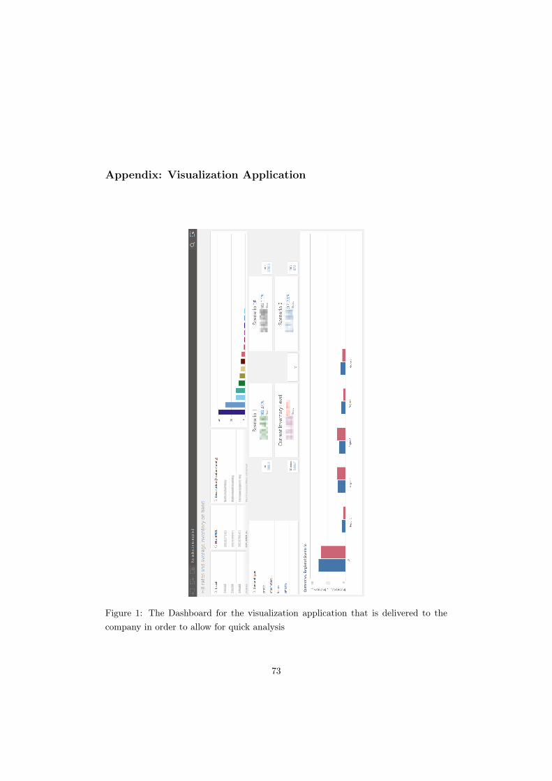
Appendix: Visualization Application

Figure 1: The Dashboard for the visualization application that is delivered to thecompany in order to allow for quick analysis

73

Figure 2: Another view in the visualization application that shows a drill-down anal-ysis

74