Finnish Centre for PensionsWorking Papers 7

Age-Wage Profiles for Finnish Workers

Kalle Elo, Finnish Centre for PensionsJanne Salonen, Finnish Centre for Pensions

Helsinki 2004 ISSN 1458-753XISBN 951-691-021-1

Contents

Abstract ........................................................................................................... 7

Introduction..................................................................................................... 9

Data................................................................................................................ 11

Estimation ..................................................................................................... 20Model Selection 23Results 26

Forecasting ................................................................................................... 27In-sample forecast - 1994–2001 29Out-of-sample forecast - 2002–2010 32An application to cross-section forecasting 38A preliminary test 40Male-female wage difference in the future 41

Conclusion .................................................................................................... 43

References .................................................................................................... 44

Appendix

TIIVISTELMÄ

Tässä selvityksessä pyritään mallintamaan ja ennustamaan TEL-vakuutettu-jen palkkojen kehitys iän mukaan. Selvityksessä sovelletaan perinteistä Box-Jenkinsin aikasarjamenetelmää, ja ennusteiden luotettavuutta on pyritty paran-tamaan ennusteita yhdistämällä. Aineisto käsittää suurimpien työeläkeyhtiöi-den TEL-vakuutettujen palkat 18–60-vuotiaille miehille ja naisille. Aineisto kat-taa vuodet 1966–2001 ja se edustaa 70–95% TEL-vakuutetusta palkasta ky-seisenä aikana. Tulokset viittaavat naisten osalta selvästi siihen, että lähivuo-sina jatkuu 1990-luvun alun laman jälkeinen trendi. Nuoret, alle kolmekymppi-set jäävät jonkin verran jälkeen yleisen ansiotasoindeksin mukaisesta kehityk-sestä. Muilla naisilla aina 60 ikävuoteen asti palkkakehitys näyttää ylittävän yleisen ansiokehityksen. Miesten osalta tulokset osoittavat pääosin päinvas-taista kehitystä. Voidaan todeta, että valtaosa miehistä, aina 49 ikävuoteen asti, jää jonkin verran jälkeen yleisestä ansiokehityksestä. 30–39-vuotiailla en-nusteet erosivat toisistaan, ja ennusteiden yhdistelynkin jälkeen kehityssuunta jäi epäselväksi. Vanhemmilla miehillä, 50 ikävuoden jälkeen, palkat näyttäisi-vät kasvavan yleistä ansiokehitystä nopeammin. Nämä tulokset seuraavat an-siokehityksen pitkän aikavälin trendistä. Toinen tulos, jolle saattaa olla käyttöä eläkepolitiikan suunnittelussa on se, että naiset saavuttavat hitaasti mutta varmasti miehiä palkkakehityksessä.

7

ABSTRACT

This study will apply the Box–Jenkins methodology model to estimate and forecast age-earnings profiles for Finnish workers. Estimation is done in a standard ARIMA framework with regressors of real economic growth and pre-vious wages. The forecasting is based on pure time series modelling. As known, time-series models are subject to past history. However, it seems that for all ages a reasonably simple model can be found, but no one model can be applied to all ages. This is even more true when men and women are studied separately. Forecast combination provides new information for forecasting fu-ture wages. Simple combining methodology, i.e. average and median, improve in-sample forecast accuracy significantly. This is expected to give reliable fore-casts for the future too.

8

9

INTRODUCTION

In modelling the economy one needs thorough knowledge of the underlying factors and their future development. This is important in generational model-ling. In all economically motivated overlapping-generations models it is impor-tant to know how people’s age-income profiles develop. The Finnish Centre for Pensions’ long-term pension expenditure model is the prime motivating factor for this study. It is important to know and to predict the underlying wage his-tory. What is the right retirement wage and how will it develop in the future? Knowledge of the age-income profiles is important generally as well.

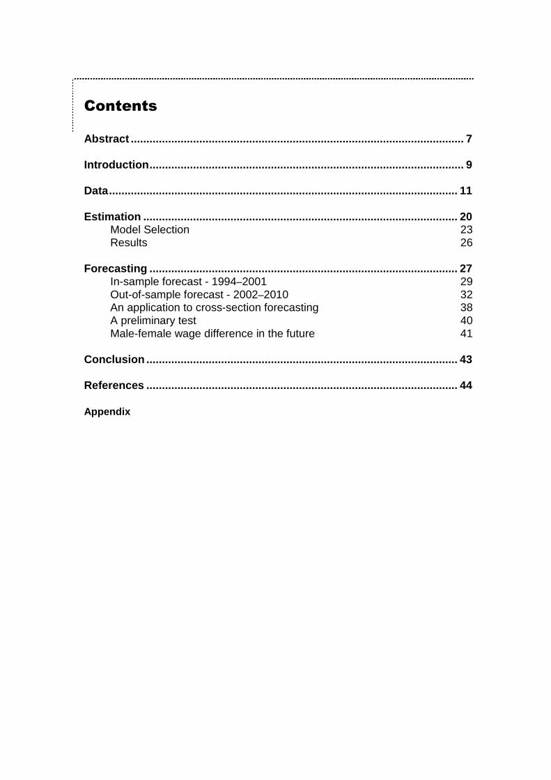
It can be seen that age-income profiles have changed dramatically over the last decades in Finland (Figure 1). The change was especially clear in the 1990s. The wages of the younger generations have fallen by several per cent in real terms in reference to older generations. It is, however, presumable that it is a temporary phenomenon and that the demographic and economic forces will increase the wages of the young generations. Another interesting question is women’s wages. Will women catch up with men in the wage development?

The availability of the data makes it possible to study this issue and possiblyadd to the number of income studies in Finland (See for example Nygård (1989), Pehkonen & Virén (1992), Asplund (1993, 1997), Hietala (1995) and Lappeteläinen (1994)). Traditionally income studies have been based on indi-vidual data. This study is based on aggregate data and time-series methods (Discussion of traditional methods in other words regression analysis is found in Freeman (1989) and Deaton (1997)).

10

Figure 1. Cross-section wages for men (top) and women (bottom) at 2001 prices.

The structure of this paper is the following. First, we describe the data and its manipulations. Second, we build a model, which complies with time-series modelling and traditional regression modelling. The aim is to fit the best model to the data for the time period 1966 to 2001. This model also indicates the structure for the forecast model. Third, we build a forecast model, aiming to predict future wages. The best models are tested against each other and the actual data. Out-of-the-sample forecasts conclude our exercise.

0

500

1000

1500

2000

2500

3000

3500

18 25 32 39 46 53 60Age

€/m

on

th

1966

1985

2001

0

500

1000

1500

2000

2500

18 25 32 39 46 53 60Age

€/m

on

th

1966

1985

2001

11

DATA

The data available to us are somewhat unique. They cover the period from 1966 to 2001. They give a nice cross-section view of the last decades with fluctuations of the economy and demography. The data, kindly provided to us by the largest pension insurance companies1, include the following information.

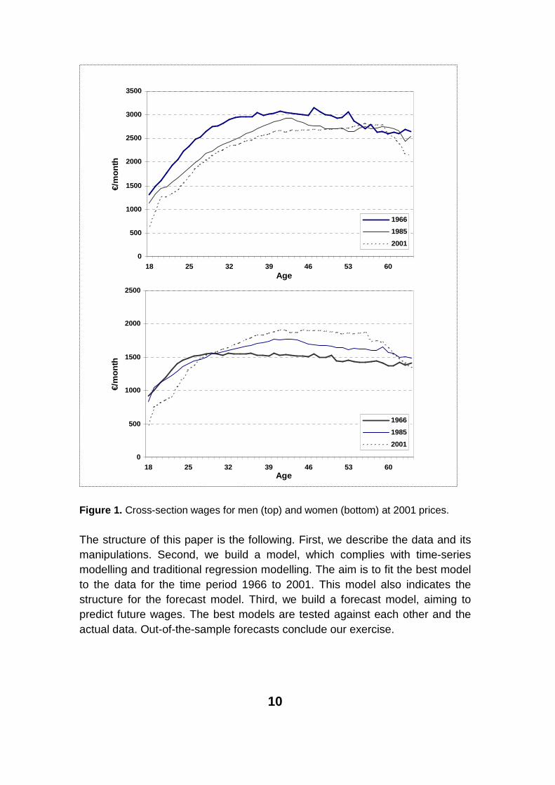
The wage information relates to people insured under TEL (the Employees’ Pensions Act) aged 15 to 65. The wage concept is the annual wage that the employer reports to the companies. We do not have any other income informa-tion. The terms wage and income are used here in the same sense. The data show the end-of-the-year situation. Information is also available by gender. There is, on the other hand, no further information on the occupation or sector.The number of insured is available for all the age categories as well. We will not use that information in this study, however.

Figure 2. Total number of persons insured under TEL in the major pension insurance companies.

1 The data cover roughly 70–95% of the wages insured under TEL in the pension insurance companies.

0

200000

400000

600000

800000

1000000

1200000

66 71 76 81 86 91 96 01

Year

Fre

qu

ency

Men Women Total

12

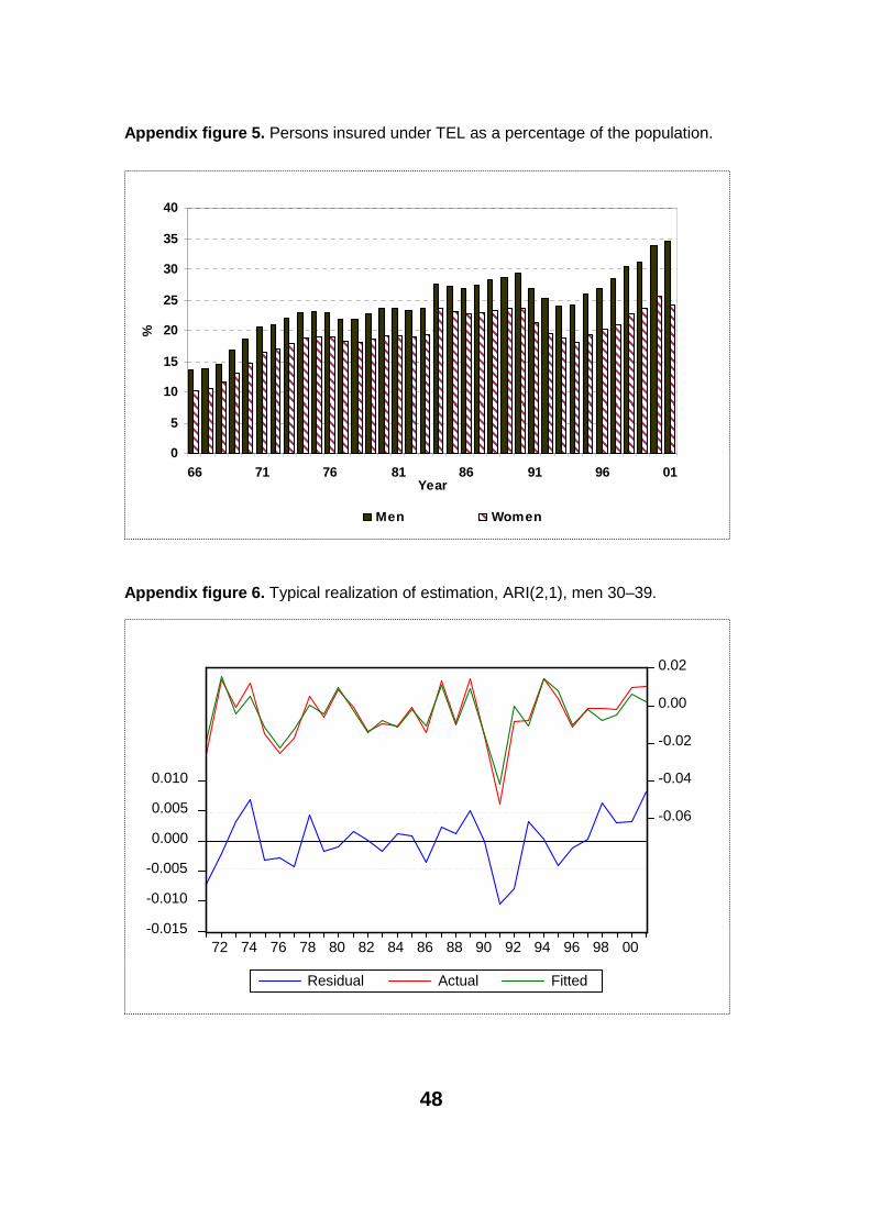
Since the data come from administrative records, there is naturally some varia-tion in the definition2 of wages. For example, in the early years the employmentcontract limit may have excluded some young people. Still, in figure 2 it has not shown up in 1972. It can also be seen that the number of women in rela-tion to the number of men has been very stable, as can be seen in figure 2(appendix figure 5 shows a corresponding figure as a percentage of the popu-lation). This is even more notable since women usually work in the public sec-tor, and public sector employers are not included in our data. However, these issues do not greatly affect the data. The statistical method is also quite insen-sitive for these early years.

There are some deficiencies in the data. Wages are aggregates of all age categories. There is no additional information on the underlying ‘work effort’ so one can not say much about the working hours.3 Although we make notations of cohort effects, there are no individual people in the data. The data consist of 36 cross-sections added together, so one could describe it as a ‘pseudo panel’.

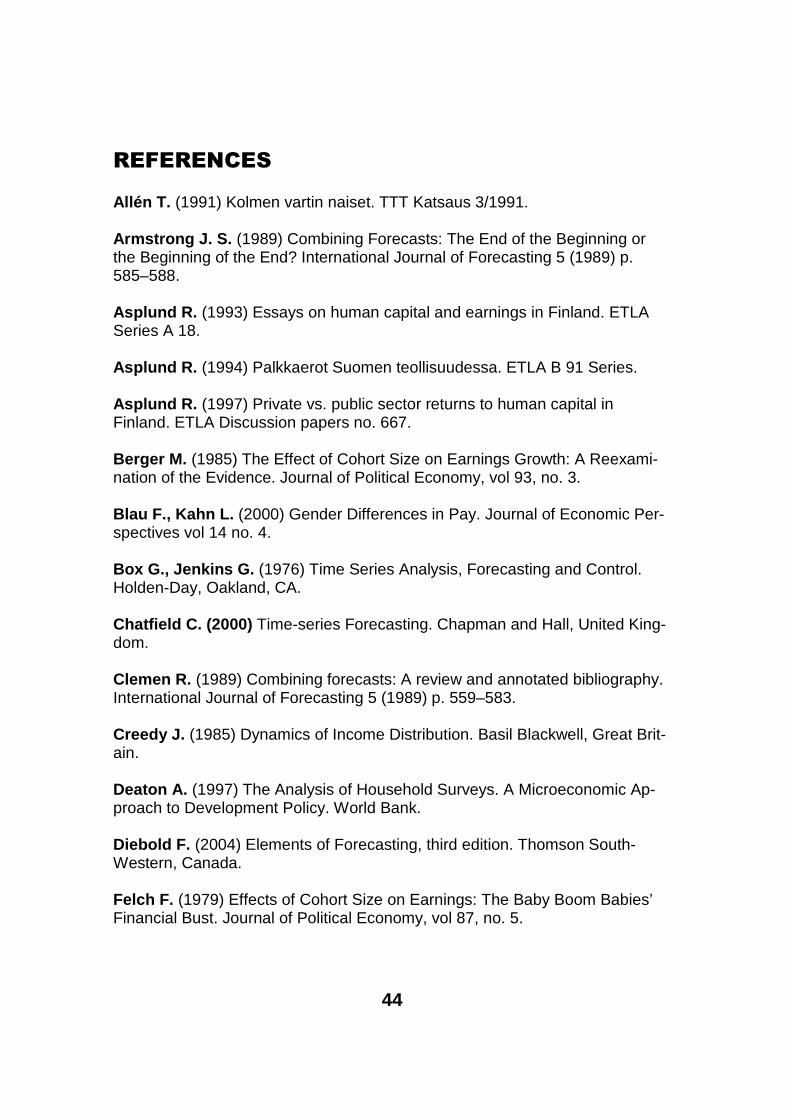
In addition to wage information, we used a simple variable indicating overall economic performance, the yearly change in (or growth in) real GDP. Appendix figure 1 shows how this indicator has evolved throughout the years. The re-cession of the ‘90s was serious in the Finnish economy. It should be noticed that between the ‘60s and the ‘70s there were also great fluctuations in the economy. These early years were challenging in our estimations too.

An additional motivation for this real economy indicator is that it can be used when we estimate future wages.

Based on this information, we will describe and analyse age-specific wages for men and women separately. In the analysis part we will try to fit a reasonable model to the data and try to predict the future. For the analysis we will need to construct additional explanatory variables. In this kind of study there are usu-ally variables that describe the state of the economy, unemployment, educa-tion, cohort and work experience. Some of these we can construct from the

2 The earnings limit for men as a percentage of the sample mean was roughly 20% between 1966 and 1973 (36% for women). After that it has remained at roughly 10% (15% for women). The minimum length of the employment contract was 4 months between 1 January 1965 and 1 July 1971. After that it has been 1 month. Additionally the employment contract must be valid at the end of the year to be recorded in the data.

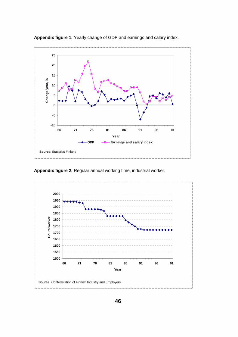
3 In general working hours have decreased constantly during the period 1966 to 2001. As can be seen from appendix figure 2 the industrial workers’ working hours have decreased by over 200 hours per year. The level of working hours is currently near the EU average.

13

data, but some we cannot. For predictive purposes one needs to be careful with the chosen model. A simple model is our preference. We will try this, and keeping in mind the key questions, we will be able to say something about the future.

Before we take a look at the data, we must look at some issues concerning data manipulation. We must also understand how the structure of the economy has changed over the past few decades, and how it might influence our find-ings.

Age groups, indexation and randomness of the data

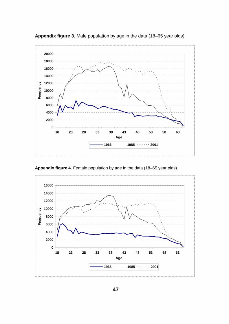
There are several data manipulation steps before the actual analysis can be-gin. First, we check the wage series for each age from 15 to 65. We noticed that the profile changes somewhat slowly and we could base the analysis on grouped data. So there are five age groups: 20–29, 30–39, 40–49, 50–54, 55–60. Each group consists of the weighted average of the wages of the underly-ing ages. The weight is the proportion of the population in the data at each in-dividual age. The age limits 20 and 60 follow from the fact that the number of employees decrease fast beyond these ages (See appendix figures 3 and 4). Accordingly it is safer to limit the analysis to the ‘working age’ population.

Second, there is the question of how to make our data real in values? It can be done in several ways. The first candidate is the consumer price index (CPI). In this way the wages are put in proportion to price increases. The price in-crease is unilateral for all employees, and in that sense it would be a good candidate. The second way is to construct an index of the data themselves,which has a merit too. The third way (which is our choice) is to make the datareal in values by using an index of wage and salary earnings. With an earnings index we can see how the data develops vis-à-vis the general earnings devel-opment. The earnings and salary index also puts recent years into better per-spective. (For discussion in Finnish see Kettunen (1993) and Asplund (1994)).

14

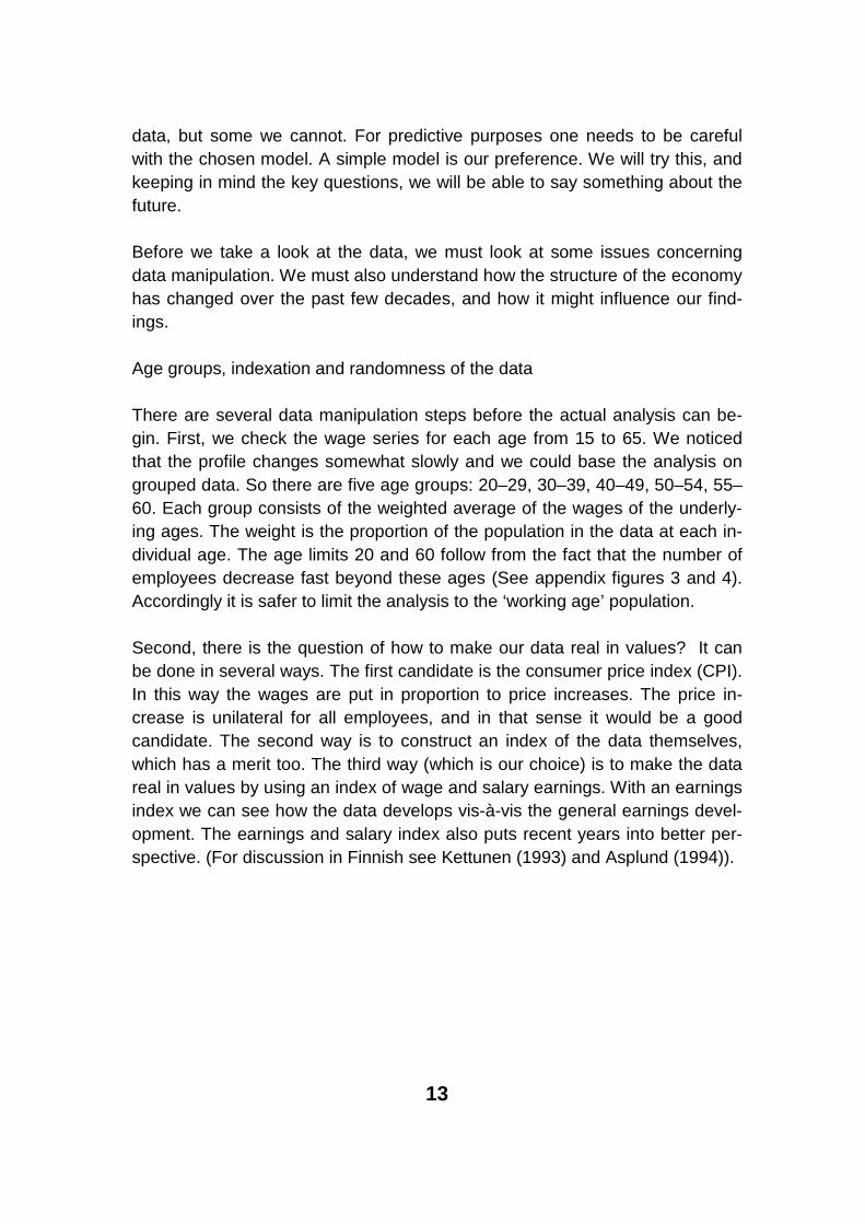
Figure 4. Average real wages for selected age groups for men. At 2001 prices.

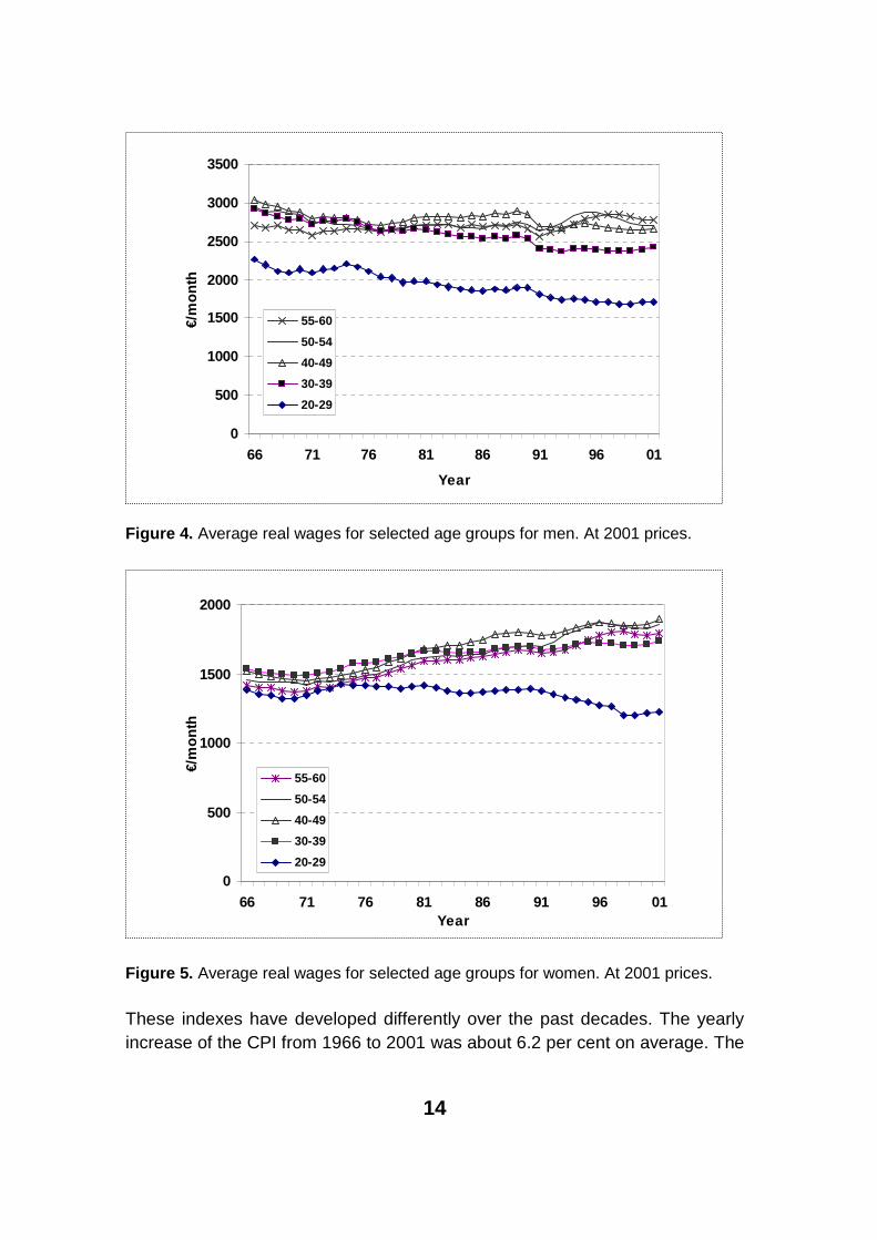
Figure 5. Average real wages for selected age groups for women. At 2001 prices.

These indexes have developed differently over the past decades. The yearly increase of the CPI from 1966 to 2001 was about 6.2 per cent on average. The

0

500

1000

1500

2000

66 71 76 81 86 91 96 01Year

€/m

on

th

55-60

50-54

40-49

30-39

20-29

0

500

1000

1500

2000

2500

3000

3500

66 71 76 81 86 91 96 01

Year

€/m

on

th

55-60

50-54

40-49

30-39

20-29

15

earnings and salary index has increased a little faster, nearly 8.5 per cent (See appendix figure 1 for graph of yearly change of the earnings and salary index). If we construct an index of average wages of the data themselves we can see that it has followed the general earnings and salary index closely. For men it has grown 0.4 percentage points slower. For women it has grown 0.5 percent-age points faster.

With different realizations we can view the wage development from various perspectives. It is plausible to think that recently, within the EMU, when prices are more stable, the earnings and salary index is a better reference point. We believe it is the right way to realize this kind of time-series data. The data ap-pear in the level for 2001. However the estimation results are not greatly af-fected by realization.

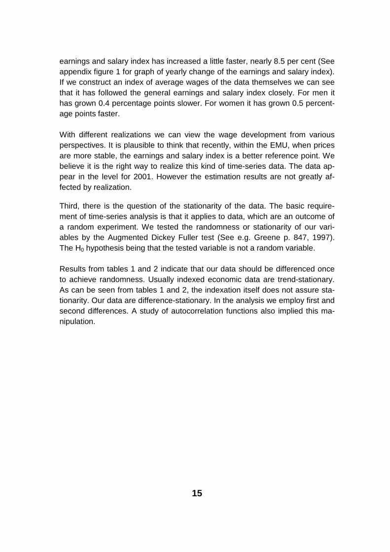
Third, there is the question of the stationarity of the data. The basic require-ment of time-series analysis is that it applies to data, which are an outcome of a random experiment. We tested the randomness or stationarity of our vari-ables by the Augmented Dickey Fuller test (See e.g. Greene p. 847, 1997). The H0 hypothesis being that the tested variable is not a random variable.

Results from tables 1 and 2 indicate that our data should be differenced once to achieve randomness. Usually indexed economic data are trend-stationary. As can be seen from tables 1 and 2, the indexation itself does not assure sta-tionarity. Our data are difference-stationary. In the analysis we employ first and second differences. A study of autocorrelation functions also implied this ma-nipulation.

16

Table 1. Results of unit-root tests, men.

Level First difference

Variables No trend InterceptTrend &

InterceptNo trend Intercept

Trend & Intercept

Wage2029-0 lag -2.81*** -1.28 -2.31 -4.16*** -4.57*** -4.49***-1 lag -1.67* -0.80 -3.37* -3.65*** -4.06*** -3.97**

Wage3039-0 lag -2.26** -1.77 -2.62 -4.93*** -5.37*** -5.43***-1 lag -1.76* -1.46 -3.01 -3.44*** -3.79*** -3.82**

Wage4049-0 lag -1.46 -2.38 -2.44 -5.13*** -5.24*** -5.20***-1 lag -1.07 -2.08 -2.38 -3.17*** -3.24** -3.22*

Wage5054-0 lag -0.89 -2.67* -2.49 -5.10*** -5.06*** -5.02***-1 lag -0.50 -2.33 -2.26 -3.07*** -3.07** -3.10

Wage5560-0 lag 0.29 -2.67* -2.49 -5.55*** -5.49*** -5.42***-1 lag 0.39 -1.72 -2.54 -3.23*** -3.17** -3.16

Table 2. Results of unit-root tests, women.

Level First difference

Variables No trend InterceptTrend &

InterceptNo trend Intercept

Trend & Intercept

Wage2029-0 lag -1.46 0.21 -0.80 -3.89*** -3.89*** -4.21**-1 lag -0.64 -0.61 -1.79 -2.74 -2.74 -3.09

Wage3039-0 lag 2.22 -0.31 -1.70 -3.58*** -4.18*** -4.12**-1 lag 1.97 -0.98 -2.06 -2.45 -3.09 -3.09

Wage4049-0 lag 3.35 0.30 -2.31 -2.61** -3.64*** -3.56**-1 lag 2.44 -0.54 -2.14 -1.51 -2.54 -2.49

Wage5054-0 lag 3.73 0.31 -2.80 -3.06*** -4.18*** -4.13**-1 lag 2.59 -0.24 -2.95 -1.88 -2.85 -2.78

Wage5560-0 lag 3.52 0.11 -2.56 -3.11*** -4.10*** -4.01**-1 lag 2.41 -0.57 -2.85 -2.04 -2.89 -2.81

Note for tables 1 and 2: ***, ** and * indicate significance at the 1%, 5% and 10% levels. The McKinnon critical val-ues of ADF statistics (level) are:-2.6, -2.0 and -1.6 without trend; -3.6, -2.9 and -2.6 with intercept; -4.2, -3.5 and -3.2 with trend and intercept at the 1%, 5% and 10% levels of significance, respectively. For the first difference some of the critical values are slightly smaller.

We conclude our data manipulation by stating that the GDP change variable rejected the ADF null hypothesis at the 5% risk level.

17

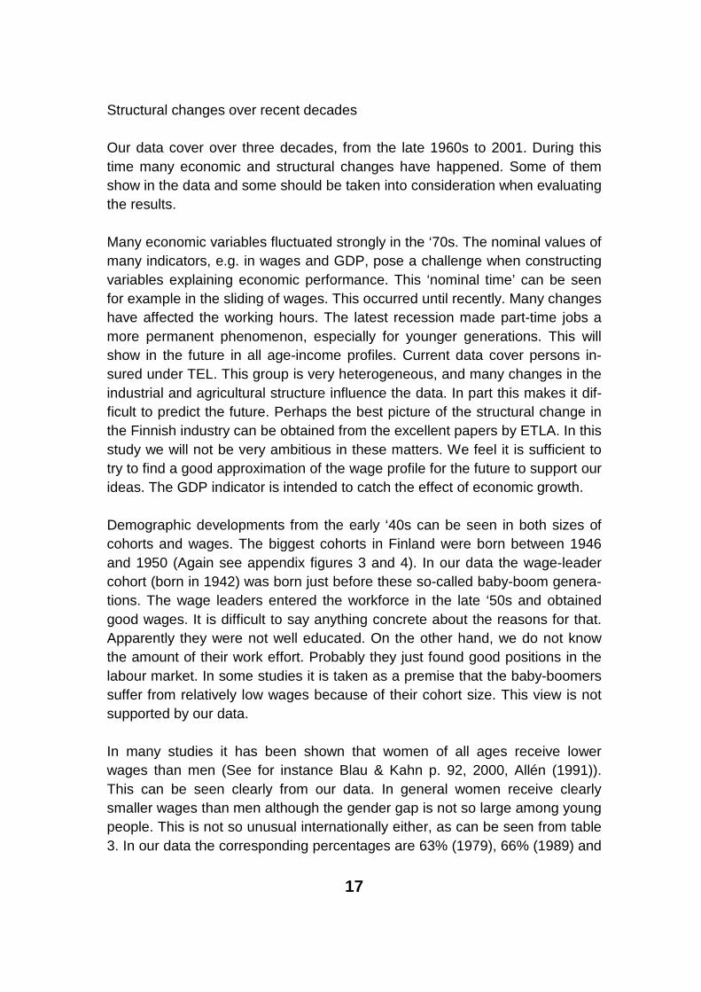
Structural changes over recent decades

Our data cover over three decades, from the late 1960s to 2001. During this time many economic and structural changes have happened. Some of themshow in the data and some should be taken into consideration when evaluating the results.

Many economic variables fluctuated strongly in the ‘70s. The nominal values of many indicators, e.g. in wages and GDP, pose a challenge when constructing variables explaining economic performance. This ‘nominal time’ can be seen for example in the sliding of wages. This occurred until recently. Many changes have affected the working hours. The latest recession made part-time jobs a more permanent phenomenon, especially for younger generations. This will show in the future in all age-income profiles. Current data cover persons in-sured under TEL. This group is very heterogeneous, and many changes in the industrial and agricultural structure influence the data. In part this makes it dif-ficult to predict the future. Perhaps the best picture of the structural change in the Finnish industry can be obtained from the excellent papers by ETLA. In this study we will not be very ambitious in these matters. We feel it is sufficient to try to find a good approximation of the wage profile for the future to support our ideas. The GDP indicator is intended to catch the effect of economic growth.

Demographic developments from the early ‘40s can be seen in both sizes of cohorts and wages. The biggest cohorts in Finland were born between 1946and 1950 (Again see appendix figures 3 and 4). In our data the wage-leader cohort (born in 1942) was born just before these so-called baby-boom genera-tions. The wage leaders entered the workforce in the late ‘50s and obtainedgood wages. It is difficult to say anything concrete about the reasons for that. Apparently they were not well educated. On the other hand, we do not know the amount of their work effort. Probably they just found good positions in the labour market. In some studies it is taken as a premise that the baby-boomers suffer from relatively low wages because of their cohort size. This view is not supported by our data.

In many studies it has been shown that women of all ages receive lower wages than men (See for instance Blau & Kahn p. 92, 2000, Allén (1991)). This can be seen clearly from our data. In general women receive clearly smaller wages than men although the gender gap is not so large among young people. This is not so unusual internationally either, as can be seen from table 3. In our data the corresponding percentages are 63% (1979), 66% (1989) and

18

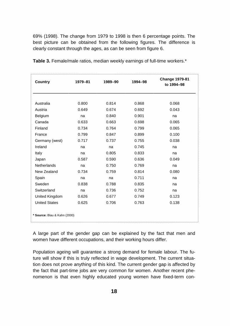
69% (1998). The change from 1979 to 1998 is then 6 percentage points. The best picture can be obtained from the following figures. The difference is clearly constant through the ages, as can be seen from figure 6.

Table 3. Female/male ratios, median weekly earnings of full-time workers.*

Country 1979–81 1989–90 1994–98Change 1979-81

to 1994–98

Australia 0.800 0.814 0.868 0.068

Austria 0.649 0.674 0.692 0.043

Belgium na 0.840 0.901 na

Canada 0.633 0.663 0.698 0.065

Finland 0.734 0.764 0.799 0.065

France 0.799 0.847 0.899 0.100

Germany (west) 0.717 0.737 0.755 0.038

Ireland na na 0.745 na

Italy na 0.805 0.833 na

Japan 0.587 0.590 0.636 0.049

Netherlands na 0.750 0.769 na

New Zealand 0.734 0.759 0.814 0.080

Spain na na 0.711 na

Sweden 0.838 0.788 0.835 na

Switzerland na 0.736 0.752 na

United Kingdom 0.626 0.677 0.749 0.123

United States 0.625 0.706 0.763 0.138

* Source: Blau & Kahn (2000)

A large part of the gender gap can be explained by the fact that men and women have different occupations, and their working hours differ.

Population ageing will guarantee a strong demand for female labour. The fu-ture will show if this is truly reflected in wage development. The current situa-tion does not prove anything of this kind. The current gender gap is affected by the fact that part-time jobs are very common for women. Another recent phe-nomenon is that even highly educated young women have fixed-term con-

19

tracts. This will influence their life-long wage profile and they will probably never catch up with young men.

Figure 6. The gender gap in wages in 1971, 1985 and 2001.

The previous reasoning was based on the situation of supply and demand inthe labour market, and the resultant wage and employment equilibrium. There is also another possible framework, which does not pose a good picture for women. Women usually work in occupations where productivity of the worker is low. This does not seem to change in the future either.

0,0

0,1

0,2

0,3

0,4

0,5

0,6

0,7

0,8

0,9

1,0

18 24 30 36 42 48 54 60

Age

Fem

ale/

Mal

e

1971

1985

2001

20

ESTIMATION

The aim of this chapter is to construct and fit a statistical model to the data. Since there is a notable difference in wages for men and for women, we begin to search for gender-specific data. We began with a wide range of models in the AR, MA and ARIMA family.

It soon became clear that high-order models were not the best choice. For ex-ample a third-order model did not converge in a satisfactory way. Second, we wanted to have the real regressors in the models. The reason for this was that the pure AR, MA or ARIMA models did not work very well on their own.

The AR, MA and ARMA models are most tractable expressed in the general form. The formulations follow Box & Jenkins (1976) and Diebold (2004). How-ever, the notation is ours.

An autoregressive model, which essentially is a simple mathematical model in which the current value of a series (Wage, W), is linearly related to its past val-ues plus an additive stochastic shock. Simple univariate AR(1) can be ex-pressed as:

ttt WW εφ += −11 . (1)

Critical assumptions require also white noise errors, ),0(~ 2σε WNt and 11 1 <<− φ for the stationary process. In lag operator form (1) can be ex-

pressed as:

ttWL εφ =− )1( . (2)

Note that:

1)1( −−=−=− ttttt WWLWWWL φφφ . (3)

Thus, model (2) is equivalent to (1). In a similar fashion we can express the AR(2) model as:

tttt WWW εφφ ++= −− 211 . (4)Note that the lag operator can now be expressed as:

21

ttt WLLWL εφφ =−−=Φ )1()( 221 , (5)

where critical assumptions require white noise errors, ),0(~ 2σε WNt and 1,1 1221 <−<+ φφφφ and 11 2 <<− φ . The AR(2) process is covariance-

stationary if the inverses of all roots of the autoregressive lag-operator poly-nomial )(LΦ are inside the unit circle. A necessary condition for covariance-stationarity is 11 <Σ = i

pi φ (See Diebold p. 156, 2004 for discussion).

The moving average process is based on the idea that a stochastic series (like ours) can be modelled as distributed lags of current and past shocks. One property of the MA process is that low-degree models have relatively short memory regardless of parameter values.

A first-order moving average, the MA(1) process can be expressed as:

tttt LW εθθεε )1(1 +=+= − . (6)

Critical assumptions also require white noise errors, ),0(~ 2σε WNt . The proc-ess is covariance-stationary for any parameter values. If 1<θ the MA(1) proc-ess is invertible (See Diebold p. 150, 2004 for discussion). The MA(2) process is a natural generalization on the MA(1) process. Allowing more lags on the right side of the equation, the MA(2) process can capture richer dynamic pat-terns.

The MA(2) process can in a similar way be expressed as:

ttttt LW εεθεθε )(2211 Θ=++= −− , (7)

where critical assumptions also require white noise errors, ),0(~ 2σε WNt .The lag operator can now be expressed as:

.1)( 221 LLL θθ ++=Θ (8)

The next step is to present a combination of the AR and MA components. The simplest ARMA process can be expressed as:

11 −− ++= tttt WW θεεφ . (9)Critical assumptions also require white noise errors, ),0(~ 2σε WNt . In lag op-erator form (9) can be expressed as:

22

tt LWL εθφ )1()1( +=− . (10)

where 1<φ is required for stationarity and 1<θ for invertibility. When these conditions are met the process can be expressed in autoregressive form as:

tt L

LW ε

φθ

)(

)(= . (11)

The next step is to take the differences of the data. We use the following nota-tion of the wage variable:

1−−=∆ ttt WWW

12

−∆−∆=∆ ttt WWW

213

−− ∆−∆=∆ ttt WWW

After the wage variable was made stationary by the first-order differencing, the above pure time-series models were employed. The results were not promis-ing. The next step was to add ‘real wage’ regressors tW2∆ and tW3∆ to the models. A GDP regressor and a constant (c) were also added to the models.

Estimated model for the years 1966–2001

Using the EViews program we estimated the following time-series models with regressors. We also tried other formulations in these families. Still, the parsi-mony principle seemed to reduce the models to these simple variants.

First is an ARI (1,1) type model:

ttttttt WBKTWWcW εφ +∆+∆+∆+∆+=∆ −132 . (12)

Second is an ARI (2,1) type model:

tttttttt WWBKTWWcW εφφ +∆+∆+∆+∆+∆+=∆ −− 221132 . (13)

Third is an ARIMA (1,1,1) type:

111132

−− ++∆+∆+∆+∆+=∆ ttttttt WBKTWWtcW εθεφ . (14)

23

Model Selection

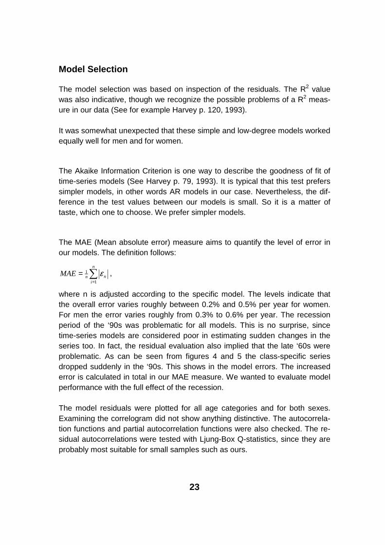
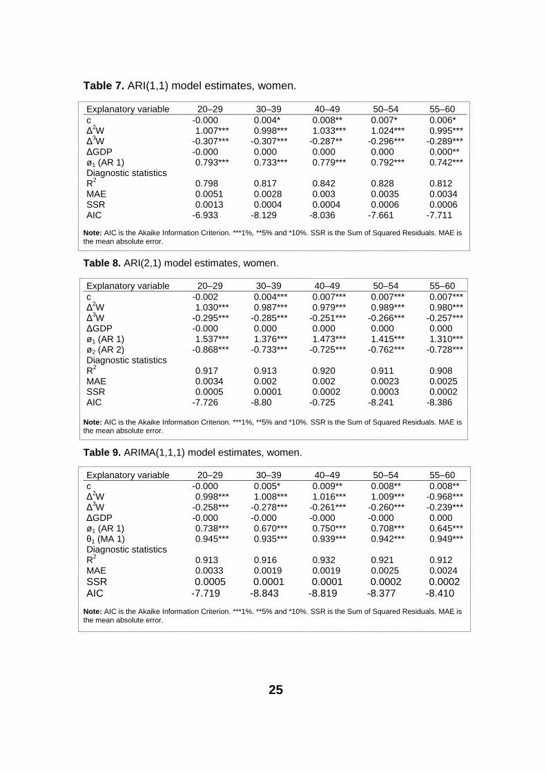
The model selection was based on inspection of the residuals. The R2 value was also indicative, though we recognize the possible problems of a R2 meas-ure in our data (See for example Harvey p. 120, 1993).

It was somewhat unexpected that these simple and low-degree models worked equally well for men and for women.

The Akaike Information Criterion is one way to describe the goodness of fit of time-series models (See Harvey p. 79, 1993). It is typical that this test prefers simpler models, in other words AR models in our case. Nevertheless, the dif-ference in the test values between our models is small. So it is a matter of taste, which one to choose. We prefer simpler models.

The MAE (Mean absolute error) measure aims to quantify the level of error in our models. The definition follows:

∑=

=n

innMAE

1

1 ε ,

where n is adjusted according to the specific model. The levels indicate that the overall error varies roughly between 0.2% and 0.5% per year for women. For men the error varies roughly from 0.3% to 0.6% per year. The recession period of the ‘90s was problematic for all models. This is no surprise, since time-series models are considered poor in estimating sudden changes in the series too. In fact, the residual evaluation also implied that the late ‘60s were problematic. As can be seen from figures 4 and 5 the class-specific series dropped suddenly in the ‘90s. This shows in the model errors. The increased error is calculated in total in our MAE measure. We wanted to evaluate model performance with the full effect of the recession.

The model residuals were plotted for all age categories and for both sexes. Examining the correlogram did not show anything distinctive. The autocorrela-tion functions and partial autocorrelation functions were also checked. The re-sidual autocorrelations were tested with Ljung-Box Q-statistics, since they are probably most suitable for small samples such as ours.

24

Table 4. ARI(1,1) model estimates, men.

Explanatory variable 20–29 30–39 40–49 50–54 55–60c -0.007 -0.008*** -0.005* -0.004 -0.002∆2W -0.912*** 0.815*** 0.853*** 0.865*** 0.897***∆3W -0.272** -0.226** -0.234*** -0.227** -0.247***∆GDP 0.000 0.001*** 0.001*** 0.001** 0.001***ø1 (AR 1) 0.607*** 0.425** 0.660*** 0.772*** 0.730***Diagnostic statisticsR2 0.771 0.849 0.860 0.823 0.854MAE 0.0063 0.0042 0.0043 0.005 0.0044SSR 0.0019 0.00097 0.00095 0.0014 0.001AIC -6.578 -7.252 -7.270 -6.886 -7.180

Note: AIC is the Akaike Information Criterion. ***1%, **5% and *10%. SSR is the Sum of Squared Residuals. MAE is the mean absolute error.

Table 5. ARI(2,1) model estimates, men.

Explanatory variable 20–29 30–39 40–49 50–54 55–60c -0.007* -0.005*** -0.003 -0.002 0.000∆2W 1.016*** 0.997*** 0.983*** 0.950*** 0.960***∆3W -0.282*** -0.271*** -0.264*** -0.243*** -0.253***∆GDP -0.000 0.000 0.000 0.000 0.000ø1 (AR 1) 1.223*** 1.080*** 1.200*** 1.285*** 1.221***ø2 (AR 2) -0.720*** -0.768*** -0.693*** -0.740*** -0.702***Diagnostic statisticsR2 0.896 0.913 0.902 0.9000 0.907MAE 0.0042 0.0032 0.0037 0.0032 0.0033SSR 0.0008 0.0005 0.0006 0.0007 0.0006AIC -7.335 -7.714 -7.525 -7.349 -7.533

Note: AIC is the Akaike Information Criterion. ***1%, **5% and *10%. SSR is the Sum of Squared Residuals. MAE is the mean absolute error.

Table 6. ARIMA(1,1,1) model estimates, men.

Explanatory variable 20–29 30–39 40–49 50–54 55–60c -0.004 -0.004 -0.004 -0.001 0.001∆2W 0.978*** 0.952*** 0.943*** 0.982*** 0.971***∆3W -0.248*** -0.238*** -0.238*** -0.248*** -0.242***∆GDP -0.000 0.000 0.000 0.000 0.000ø1 (AR 1) 0.642*** 0.518** 0.563*** 0.638*** 0.570***θ1 (MA 1) 0.989*** 0.944*** 1.248*** 0.961*** 0.989***Diagnostic statisticsR2 0.906 0.909 0.938 0.913 0.914MAE 0.0035 0.0032 0.0028 0.0035 0.0031SSR 0.0007 0.0005 0.0004 0.0006 0.0006AIC -7.41 -7.693 -8.030 -7.531 -7.655

Note: AIC is the Akaike Information Criterion. ***1%, **5% and *10%. SSR is the Sum of Squared Residuals. MAE is the mean absolute error.

25

Table 7. ARI(1,1) model estimates, women.

Explanatory variable 20–29 30–39 40–49 50–54 55–60c -0.000 0.004* 0.008** 0.007* 0.006*∆2W 1.007*** 0.998*** 1.033*** 1.024*** 0.995***∆3W -0.307*** -0.307*** -0.287** -0.296*** -0.289***∆GDP -0.000 0.000 0.000 0.000 0.000**ø1 (AR 1) 0.793*** 0.733*** 0.779*** 0.792*** 0.742***Diagnostic statisticsR2 0.798 0.817 0.842 0.828 0.812MAE 0.0051 0.0028 0.003 0.0035 0.0034SSR 0.0013 0.0004 0.0004 0.0006 0.0006AIC -6.933 -8.129 -8.036 -7.661 -7.711

Note: AIC is the Akaike Information Criterion. ***1%, **5% and *10%. SSR is the Sum of Squared Residuals. MAE is the mean absolute error.

Table 8. ARI(2,1) model estimates, women.

Explanatory variable 20–29 30–39 40–49 50–54 55–60c -0.002 0.004*** 0.007*** 0.007*** 0.007***∆2W 1.030*** 0.987*** 0.979*** 0.989*** 0.980***∆3W -0.295*** -0.285*** -0.251*** -0.266*** -0.257***∆GDP -0.000 0.000 0.000 0.000 0.000ø1 (AR 1) 1.537*** 1.376*** 1.473*** 1.415*** 1.310***ø2 (AR 2) -0.868*** -0.733*** -0.725*** -0.762*** -0.728***Diagnostic statisticsR2 0.917 0.913 0.920 0.911 0.908MAE 0.0034 0.002 0.002 0.0023 0.0025SSR 0.0005 0.0001 0.0002 0.0003 0.0002AIC -7.726 -8.80 -0.725 -8.241 -8.386

Note: AIC is the Akaike Information Criterion. ***1%, **5% and *10%. SSR is the Sum of Squared Residuals. MAE is the mean absolute error.

Table 9. ARIMA(1,1,1) model estimates, women.

Explanatory variable 20–29 30–39 40–49 50–54 55–60c -0.000 0.005* 0.009** 0.008** 0.008**∆2W 0.998*** 1.008*** 1.016*** 1.009*** -0.968***∆3W -0.258*** -0.278*** -0.261*** -0.260*** -0.239***∆GDP -0.000 -0.000 -0.000 -0.000 0.000ø1 (AR 1) 0.738*** 0.670*** 0.750*** 0.708*** 0.645***θ1 (MA 1) 0.945*** 0.935*** 0.939*** 0.942*** 0.949***Diagnostic statisticsR2 0.913 0.916 0.932 0.921 0.912MAE 0.0033 0.0019 0.0019 0.0025 0.0024SSR 0.0005 0.0001 0.0001 0.0002 0.0002AIC -7.719 -8.843 -8.819 -8.377 -8.410

Note: AIC is the Akaike Information Criterion. ***1%. **5% and *10%. SSR is the Sum of Squared Residuals. MAE is the mean absolute error.

26

With lag sizes 5 the models mostly passed the test at the 5% risk level4. The correlations behaved best in the ARIMA model. There were some cases where the value of autocorrelation was near the critical value (0.254= 31

2± ). How-ever, we concluded that there is no need to change models. These simple models describe a variety of wages well, which was somewhat surprising.

Some idea of how the models generally behaved can bee seen in appendixfigure 6.

Results

As can be seen in the ARIMA model, men aged 40–49 have a high MA coeffi-cient (1.248). This has no practical meaning at this point. It only means that the model could not be used in forecasting anyway (See for instance Greene p. 829, 1998). Overall the model is stationary and the results are valid.

For ARIMA models one can also see that the AR and MA coefficients differ in a satisfactory way, in other words overparametrization is not a problem here.

The constant (c) has some role in these models. For men the effects are mixed in these models. It seems to have some statistical role in the ARI(1,1) model for the age groups 30–39 and 40–49. There is no statistically significant effect in the ARIMA model. For women there is certainly some role for the constant,especially in the AR(2,1) model. The constant has a distinctive role in forecast-ing, yet we wanted to test it in estimation as well.5

Let us finally take a critical view at the effects of GDP. For men the effect is clear only in the ARI(1,1) model. The positive coefficients indicate that wages are positively related to overall economic growth. For women this is not so ob-vious. This is a little surprising, since the original data indicate positive growth. We did some experiments with data divided into small and major employers6. For major employers the positive relation was clear both for men and for women.

4 Diebold (p. 139, 2004) argues that lag size should be near T .

5 Box & Jenkins (p. 92–93, 1976) warn about adding a constant term since it proposes a deterministic trend in the model.

6 The major employer has more than 49 employees.

27

FORECASTING

In practice predictions are almost invariably made with estimated parametersonly. However, in the last chapter the estimation was based on a time-series model with regressors, i.e. previous yearly changes of wages and GDP. That model can only be applied to estimation. The aim was to build a model using all possible wage information. Another aim was to test the importance of the GDP variable.

Forecasting is not possible in this framework. It would require forecasts of the future yearly changes in wages. We do not explore that here, but we turn our attention and analysis to pure time-series modelling. This means that we drop the real component out and start elaborating on pure time-series models such as presented in equations 1,4,6,7 and 9. Of course we tried numerous variants in the AR, MA and ARIMA families.

First we will study in-sample forecasts and their performance against observeddata. The second stage is to predict the future.

As an example of AR forecasting7 let us look at how a so-called chain rule would work in an AR(2) model. Following equation (4) it can be shown that the first period forecast is:

1211 −+ ++= ttt WWcW φφ)

. (15)

The second period forecast is:

ttt WWcW 2112 φφ ++= ++

)). (16)

The third period forecast is:

12213 +++ ++= ttt WWcW)))

φφ . (17)

This can be continued until the end of the forecast period.

7 Forecasts are naturally made on differenced data, but here we use a simpler notation.

28

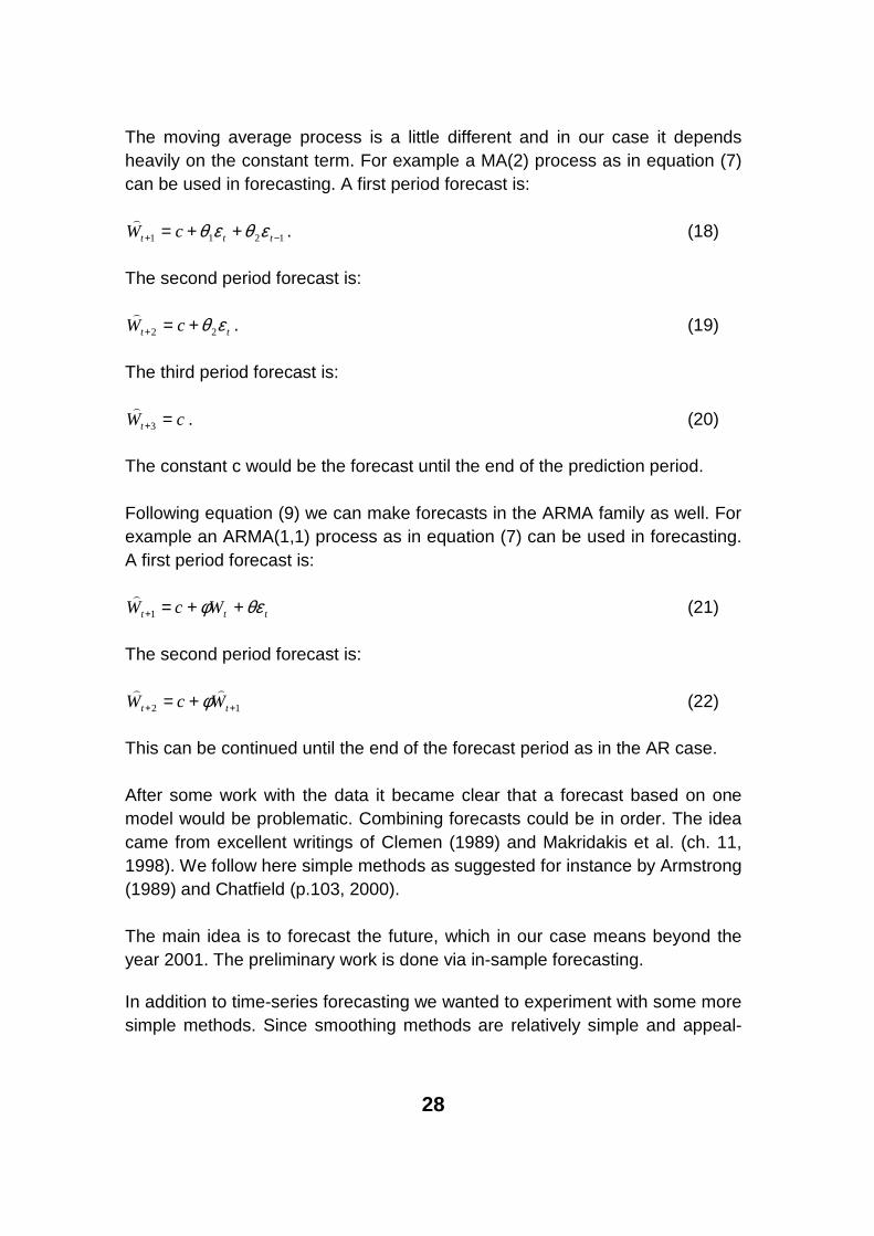
The moving average process is a little different and in our case it depends heavily on the constant term. For example a MA(2) process as in equation (7) can be used in forecasting. A first period forecast is:

1211 −+ ++= ttt cW εθεθ)

. (18) The second period forecast is:

tt cW εθ22 +=+

). (19)

The third period forecast is:

cWt =+3

). (20)

The constant c would be the forecast until the end of the prediction period.

Following equation (9) we can make forecasts in the ARMA family as well. For example an ARMA(1,1) process as in equation (7) can be used in forecasting. A first period forecast is:

ttt WcW θεφ ++=+1

)(21)

The second period forecast is:

12 ++ += tt WcW))

φ (22)

This can be continued until the end of the forecast period as in the AR case.

After some work with the data it became clear that a forecast based on one model would be problematic. Combining forecasts could be in order. The idea came from excellent writings of Clemen (1989) and Makridakis et al. (ch. 11, 1998). We follow here simple methods as suggested for instance by Armstrong (1989) and Chatfield (p.103, 2000).

The main idea is to forecast the future, which in our case means beyond the year 2001. The preliminary work is done via in-sample forecasting.

In addition to time-series forecasting we wanted to experiment with some more simple methods. Since smoothing methods are relatively simple and appeal-

29

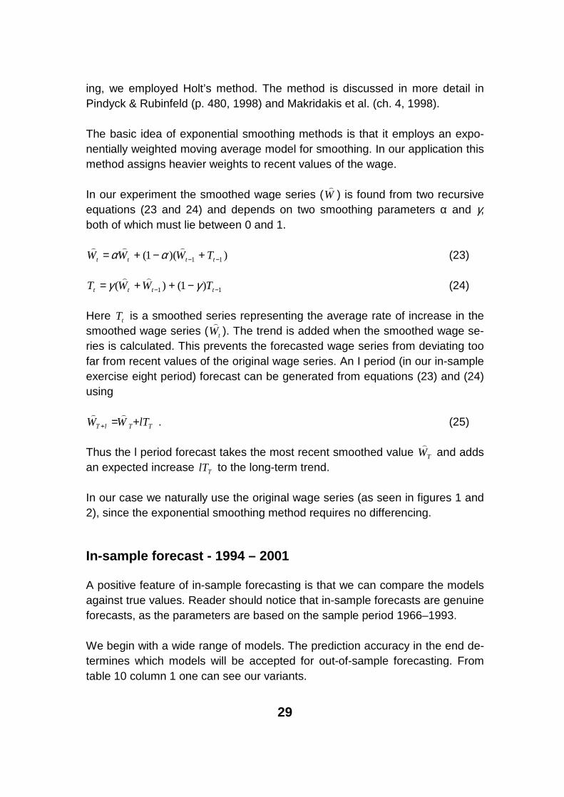
ing, we employed Holt’s method. The method is discussed in more detail in Pindyck & Rubinfeld (p. 480, 1998) and Makridakis et al. (ch. 4, 1998). The basic idea of exponential smoothing methods is that it employs an expo-nentially weighted moving average model for smoothing. In our application this method assigns heavier weights to recent values of the wage.

In our experiment the smoothed wage series (W)

) is found from two recursive equations (23 and 24) and depends on two smoothing parameters α and γ, both of which must lie between 0 and 1.

))(1( 11 −− +−+= tttt TWWW)))

αα (23)

11 )1()( −− −++= tttt TWWT γγ))

(24)

Here tT is a smoothed series representing the average rate of increase in the smoothed wage series ( tW

)). The trend is added when the smoothed wage se-

ries is calculated. This prevents the forecasted wage series from deviating too far from recent values of the original wage series. An I period (in our in-sample exercise eight period) forecast can be generated from equations (23) and (24) using

TTlT lTWW +=+

)). (25)

Thus the l period forecast takes the most recent smoothed value TW)

and adds an expected increase TlT to the long-term trend.

In our case we naturally use the original wage series (as seen in figures 1 and 2), since the exponential smoothing method requires no differencing.

In-sample forecast - 1994 – 2001

A positive feature of in-sample forecasting is that we can compare the models against true values. Reader should notice that in-sample forecasts are genuine forecasts, as the parameters are based on the sample period 1966–1993.

We begin with a wide range of models. The prediction accuracy in the end de-termines which models will be accepted for out-of-sample forecasting. From table 10 column 1 one can see our variants.

30

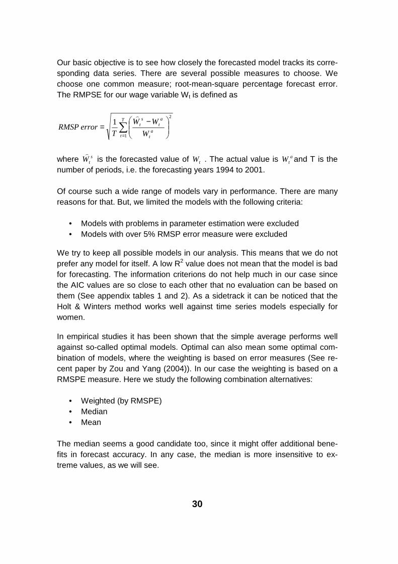
Our basic objective is to see how closely the forecasted model tracks its corre-sponding data series. There are several possible measures to choose. We choose one common measure; root-mean-square percentage forecast error. The RMPSE for our wage variable Wt is defined as

∑=

−=

T

ta

t

at

st

W

WW

TerrorRMSP

1

21

)

where stW)

is the forecasted value of tW . The actual value is atW and T is the

number of periods, i.e. the forecasting years 1994 to 2001.

Of course such a wide range of models vary in performance. There are many reasons for that. But, we limited the models with the following criteria:

• Models with problems in parameter estimation were excluded• Models with over 5% RMSP error measure were excluded

We try to keep all possible models in our analysis. This means that we do notprefer any model for itself. A low R2 value does not mean that the model is bad for forecasting. The information criterions do not help much in our case since the AIC values are so close to each other that no evaluation can be based on them (See appendix tables 1 and 2). As a sidetrack it can be noticed that the Holt & Winters method works well against time series models especially for women.

In empirical studies it has been shown that the simple average performs well against so-called optimal models. Optimal can also mean some optimal com-bination of models, where the weighting is based on error measures (See re-cent paper by Zou and Yang (2004)). In our case the weighting is based on a RMSPE measure. Here we study the following combination alternatives:

• Weighted (by RMSPE)• Median • Mean

The median seems a good candidate too, since it might offer additional bene-fits in forecast accuracy. In any case, the median is more insensitive to ex-treme values, as we will see.

31

Table 10. Root-mean-square percentage error measures for the models.*

MenModel

20-29 30-39 40-49 50-54 55-60ARI(1,1,0) 0.014 0.027 0.012 0.033 0.052ARI(2,1,0) 0.021 0.022 0.033 0.224 0.056ARI(1,2,0) 0.021 0.019 0.015 0.129 0.048ARI(2,2,0) 0.038 0.063 0.037 0.092 0.036ARIMA(1,1,1) 0.022 0.020 0.054 0.030 0.047ARIMA(2,1,1) 0.023 0.024 0.058 0.171 0.050ARIMA(1,1,2) 0.03 0.024 0.063 0.027 0.048ARIMA(2,1,2) 0.012 0.025 0.053 0.063 0.045ARIMA(1,2,1) 0.105 0.108 0.018 0.056 0.051ARIMA(2,2,1) 0.104 0.023 0.032 0.050 0.061ARIMA(1,2,2) 0.103 0.094 0.083 0.054 0.088ARIMA(2,2,2) 0.089 0.085 0.078 0.068 0.074IMA(0,1,1) 0.012 0.029 0.012 0.035 0.058IMA(0,1,2) 0.013 0.018 0.038 0.066 0.061IMA(0,2,1) 0.110 0.087 0.020 0.063 0.041IMA(0,2,2) 0.104 0.099 0.027 0.113 0.042Holt & Winters 0.042 0.050 0.031 0.033 0.059

WomenModel

20-29 30-39 40-49 50-54 55-60ARI(1,1,0) 0.063 0.018 0.034 0.028 0.030ARI(2,1,0) 0.059 0.021 0.051 0.109 0.026ARI(1,2,0) 0.019 0.034 0.050 0.125 0.027ARI(2,2,0) 0.026 0.015 0.072 0.111 0.027ARIMA(1,1,1) 0.063 0.025 0.042 0.027 0.022ARIMA(2,1,1) 0.061 0.029 0.054 0.116 0.027ARIMA(1,1,2) 0.056 0.026 0.072 0.123 0.023ARIMA(2,1,2) 0.064 0.015 0.069 0.025 0.023ARIMA(1,2,1) 0.023 0.016 0.065 0.072 0.025ARIMA(2,2,1) 0.026 0.026 0.072 0.072 0.039ARIMA(1,2,2) 0.021 0.022 0.197 0.076 0.041ARIMA(2,2,2) 0.031 0.015 0.168 0.203 0.043IMA(0,1,1) 0.067 0.013 0.016 0.019 0.033IMA(0,1,2) 0.054 0.022 0.041 0.054 0.031IMA(0,2,1) 0.027 0.021 0.034 0.065 0.043IMA(0,2,2) 0.033 0.021 0.227 0.074 0.047Holt & Winters 0.027 0.010 0.024 0.027 0.045

* Cross out indicates that the model has been dropped because of lack of significance or other problems. Italics indicate that the model has been dropped because of over 5% error. Bold indicates that the model has beenaccepted for further analysis.

32

Out-of-sample forecast - 2002 – 2010

Forecasting performance for the period 1994 to 2001 was the basis for the model selection criterion for forecasting future wages. Parameters are now re-estimated for the sample 1966–2001.

One should keep in mind that differencing a series can have a large effect on the forecast (See Makridakis et al. p. 371, 1998 and Harvey p. 115, 1993). In our case the data were differenced once, and including a constant term will lead to a linear trend forecast in the long term. This means that the forecast will follow a linear trend where the slope of the trend is equal to the fitted constant. In some cases our data are differenced twice and a constant term is included. This means that the forecast will in the long term follow a quadratic trend based on the trend at the end of the data series. This is reflected in the predic-tion intervals too. Since our approach is based on combining forecasts, we donot show the forecast variance here.8

The Holt & Winters method for real GDP growth indicates a slight growth from 1% per year in 2002 to 1.3% per year in 2010.

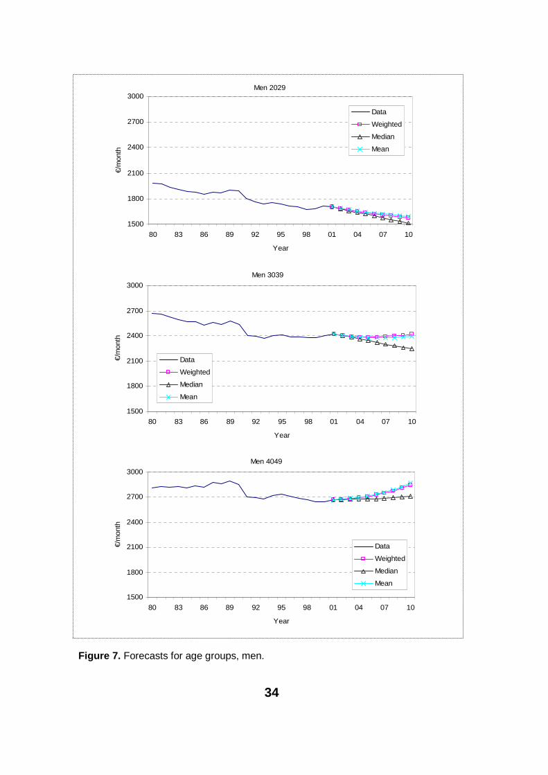
For men the results are partly expected and partly new. The downward slope for the age group 20–29 is something that one could expect from figure 4. The slight upward trend for the age groups 40–49, 50–54 and 55–60 is also ex-pected. On the other hand, the rate of growth for the age group 55–60 is sur-prising.

The three forecast-combining methods provide very uniform forecasts for the age groups 50–54 and 55–60. Our measures differ substantially for the age group 30–39. The median forecast differs from the weighted average in 2010 by roughly 7 per cent. As the weighted average predicts basically no growth between 2001 and 2010, the median forecasts a 7.2 per cent drop in wages. It seems that some models (which worked fine in the in-sample test) predict very high growth. Also, this will bend the average and weighted average upwards. The same happens in the age group 40–49. We think this is just one example why combining forecasts is necessary.

8 Chatfield (p.103, 2000) argues that there is no theoretically obvious way to compute prediction intervals.

33

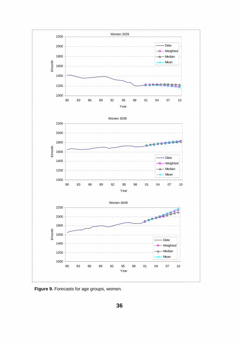
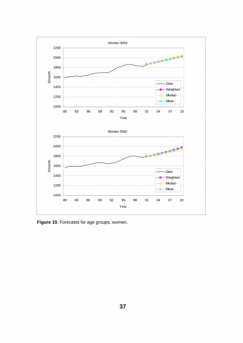
For women the methods differ only slightly. The overall data for women aretotally different from those for men, as can be seen from figures 4 and 5. Apart from the age group 20–29 there is visible growth for all age groups over the whole period. For the youngest age group there seems to be only a slight drop in relation to the wages and salary index. Our models seem to work well with women's data. Also, the downward-sloping age group 20–29 does not differ so much.

Overall the wage level for women has been lower. Still, for some time women have been converging towards men. This seems to continue in the near future. Figures 9 and 10 also show that the recession period was not so marked in this data.

34

Figure 7. Forecasts for age groups, men.

Men 2029

1500

1800

2100

2400

2700

3000

80 83 86 89 92 95 98 01 04 07 10

Year

€/m

onth

Data

Weighted

Median

Mean

Men 3039

1500

1800

2100

2400

2700

3000

80 83 86 89 92 95 98 01 04 07 10

Year

€/m

onth

Data

Weighted

Median

Mean

Men 4049

1500

1800

2100

2400

2700

3000

80 83 86 89 92 95 98 01 04 07 10

Year

€/m

onth

Data

Weighted

Median

Mean

35

Figure 8. Forecasts for age groups, men.

Men 5054

1500

1800

2100

2400

2700

3000

80 83 86 89 92 95 98 01 04 07 10

Year

€/m

onth

Data

Weighted

Median

Mean

Men 5560

1500

1800

2100

2400

2700

3000

80 83 86 89 92 95 98 01 04 07 10

Year

€/m

onth

Data

Weighted

Median

Mean

36

Figure 9. Forecasts for age groups, women.

Women 2029

1000

1200

1400

1600

1800

2000

2200

80 83 86 89 92 95 98 01 04 07 10

Year

€/m

onth

Data

Weighted

Median

Mean

Women 3039

1000

1200

1400

1600

1800

2000

2200

80 83 86 89 92 95 98 01 04 07 10

Year

€/m

onth

Data

Weighted

Median

Mean

Women 4049

1000

1200

1400

1600

1800

2000

2200

80 83 86 89 92 95 98 01 04 07 10

Year

€/m

onth

Data

Weighted

Median

Mean

37

Figure 10. Forecasts for age groups, women.

Women 5054

1000

1200

1400

1600

1800

2000

2200

80 83 86 89 92 95 98 01 04 07 10

Year

€/m

onth

Data

Weighted

Median

Mean

Women 5560

1000

1200

1400

1600

1800

2000

2200

80 83 86 89 92 95 98 01 04 07 10

Year

€/m

onth

Data

Weighted

Median

Mean

38

An application to cross-section forecasting

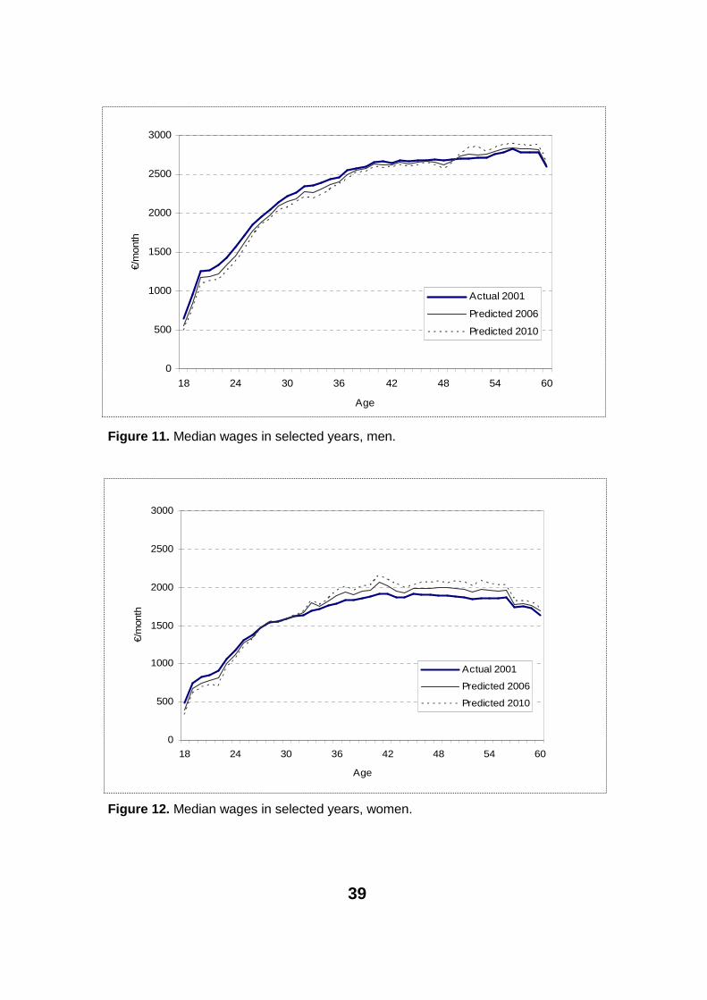
The previous models can be used to calculate age-specific forecasts. In the following we provide a median of underlying forecasts for the ages 18 to 60. As could be seen from figure 1 the cross-section profile has changed over the years. Figures 11 and 12 show how this development would continue in light of the median forecast.9 The dotted line shows the most recent data point in our analysis. The even lines show the situation some years ahead. There are sev-eral issues involved.

The first thing to notice are the ages of a drop in wages and the ages of growth in wages. There is a noticeable difference between men and women. For men the ages for which a drop will continue range from 18 to 50. Older men will gain in wages. For women this story is different. We expect some growth for women older than 30 years old.10

Second, one should notice that our yardstick is the general earnings develop-ment, which means that the growth must be above the earnings and salary index in order to show positive results here. The story would be somewhat dif-ferent with consumer price indexation. For the cohort level the story is also dif-ferent. The cohorts naturally move along these profiles and eventually they will gain even in this sort of aggregate data. The issue of cohort wages and cross-section wages is treated for example in Creedy (1985). We do not elaborate on it here.

Third, the inspection of individual model estimates revealed that some models are highly sensitive to the initial values of 2000 and 2001. Also, as the forecast period increases the forecasts explode to unlikely values. This is yet another reason to combine forecasts.

Fourth, it must be kept in mind that these phenomena are subject to structural issues in the labour market. It would be a mistake to continue these forecasts for decades. We think that some changes especially in the young age groupsare about to happen eventually. This would change these profiles notably.

9 We don’t pre-select models here. The median is calculated over all the models presented in table 10.

10 As a reference the average would predict slightly higher wages for men. For 2006 the average would be 0.5% higher and for 2010 about 2.5% higher. For women the median is slightly over in the beginning (0.2% for 2006) and then the average gets higher (0.1% for 2010).

39

0

500

1000

1500

2000

2500

3000

18 24 30 36 42 48 54 60

Age

€/m

onth

Actual 2001

Predicted 2006

Predicted 2010

Figure 11. Median wages in selected years, men.

0

500

1000

1500

2000

2500

3000

18 24 30 36 42 48 54 60

Age

€/m

onth

Actual 2001

Predicted 2006

Predicted 2010

Figure 12. Median wages in selected years, women.

40

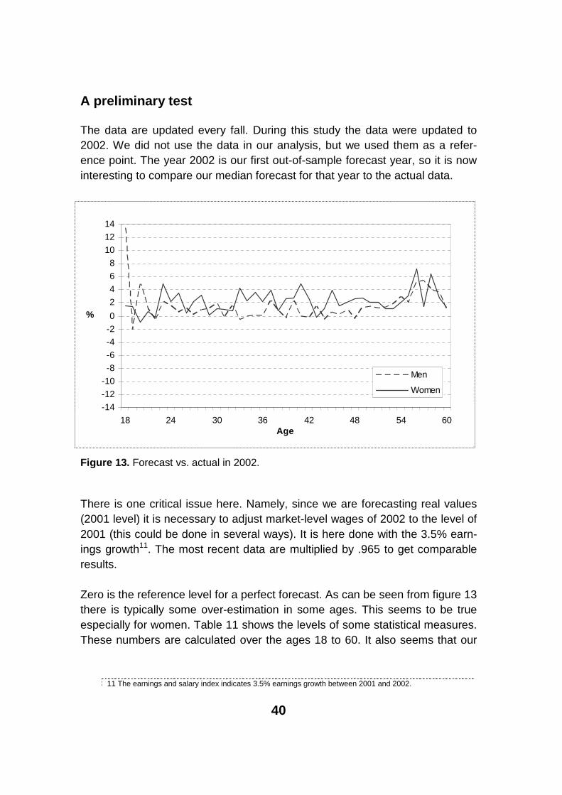
A preliminary test

The data are updated every fall. During this study the data were updated to 2002. We did not use the data in our analysis, but we used them as a refer-ence point. The year 2002 is our first out-of-sample forecast year, so it is now interesting to compare our median forecast for that year to the actual data.

-14

-12

-10

-8

-6

-4-2

0

2

4

6

8

10

12

14

18 24 30 36 42 48 54 60Age

%

Men

Women

Figure 13. Forecast vs. actual in 2002.

There is one critical issue here. Namely, since we are forecasting real values (2001 level) it is necessary to adjust market-level wages of 2002 to the level of 2001 (this could be done in several ways). It is here done with the 3.5% earn-ings growth11. The most recent data are multiplied by .965 to get comparable results.

Zero is the reference level for a perfect forecast. As can be seen from figure 13there is typically some over-estimation in some ages. This seems to be true especially for women. Table 11 shows the levels of some statistical measures. These numbers are calculated over the ages 18 to 60. It also seems that our

11 The earnings and salary index indicates 3.5% earnings growth between 2001 and 2002.

41

median forecast is too optimistic, compared to the adjusted market-level wages of 2002. Depending on the measure our median predicts roughly one per cent higher monthly wages for men, and correspondingly two per cent higher wages for women.

Table 11. Some statistics of short-term prediction performance.

Men Women

Median 1.06 2.09Mean 1.51 2.25

Male-female wage difference in the future

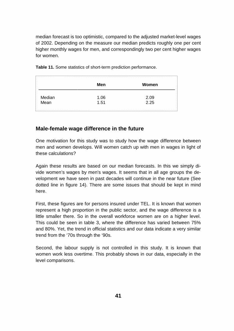
One motivation for this study was to study how the wage difference between men and women develops. Will women catch up with men in wages in light of these calculations?

Again these results are based on our median forecasts. In this we simply di-vide women’s wages by men's wages. It seems that in all age groups the de-velopment we have seen in past decades will continue in the near future (See dotted line in figure 14). There are some issues that should be kept in mind here.

First, these figures are for persons insured under TEL. It is known that women represent a high proportion in the public sector, and the wage difference is a little smaller there. So in the overall workforce women are on a higher level. This could be seen in table 3, where the difference has varied between 75% and 80%. Yet, the trend in official statistics and our data indicate a very similar trend from the ‘70s through the ‘90s.

Second, the labour supply is not controlled in this study. It is known that women work less overtime. This probably shows in our data, especially in the level comparisons.

42

Third, one should not confuse cohort effects here. Younger cohorts are more educated, especially women. Probably cohort studies would indicate a much faster narrowing wage gap. In time this will show in our cross-section data too.

Figure 14. Women’s wages in relation to men’s wages in 1971–2010.

0,2

0,4

0,6

0,8

1,0

1,2

1,4

71 74 77 80 83 86 89 92 95 98 01 04 07 10

Year

All 20-year old

40-year old 60-year old

43

CONCLUSION

Our study is a new way to study wage profiles in aggregate data. Time-series modelling has rarely been applied to study and forecast age-specific wages. Results indicate that this can be done succesfully, and reasonably simple models can be applied to all ages both for men and for women. Typically time-series modelling follows conventional rules, and with careful work this can be successful. Yet, there are some inherent problems in this approach. In this study the approach has been different. In fact we propose combining forecasts to improve accuracy.

Using several models of the AR, MA and ARIMA family we did in-sample fore-casts for the period 1994 to 2001, aiming to find reasonable models for out-of-sample forecasting of workers aged between 20 to 60 years. Three simple methods (i.e. median, average and weighted average) are presented as our out-of-sample forecasts for the years 2002 to 2010.

For women the results are uniform, the long-term trend seems to continue. A vast majority of working-age women gain in earnings growth. Results are the same regardless of the measure. For men the results are different since a ma-jority of young to middle-aged men will phase down in the wage development. The over 50 year olds are gainers in this study. The individual forecasts are however mixed for those aged between 30 and 39 years, which is the key age for earnings development, where individual models give a wide variety of fore-casts. This is why forecast combination is necessary in out-of-sample calcula-tions.

As a by-product of these forecasts we plotted the male-female wage difference as well. It seems that the gap will continue narrowing. This is probably useful information for the pension insurance industry.

Still, the question remains: Could the wage trends really continue along these lines? The statistical answer here is based on over 35 years of data. So one can only speculate on structural issues and their effects.

This study has applied a time-series approach to age-specific data. The next natural step would be to study cohort wages. Another step is to study whether cohort sizes have some effect on wages, and whether forecasts could be im-proved.

44

REFERENCES

Allén T. (1991) Kolmen vartin naiset. TTT Katsaus 3/1991.

Armstrong J. S. (1989) Combining Forecasts: The End of the Beginning or the Beginning of the End? International Journal of Forecasting 5 (1989) p. 585–588.

Asplund R. (1993) Essays on human capital and earnings in Finland. ETLA Series A 18.

Asplund R. (1994) Palkkaerot Suomen teollisuudessa. ETLA B 91 Series.

Asplund R. (1997) Private vs. public sector returns to human capital in Finland. ETLA Discussion papers no. 667.

Berger M. (1985) The Effect of Cohort Size on Earnings Growth: A Reexami-nation of the Evidence. Journal of Political Economy, vol 93, no. 3.

Blau F., Kahn L. (2000) Gender Differences in Pay. Journal of Economic Per-spectives vol 14 no. 4.

Box G., Jenkins G. (1976) Time Series Analysis, Forecasting and Control. Holden-Day, Oakland, CA.

Chatfield C. (2000) Time-series Forecasting. Chapman and Hall, United King-dom.

Clemen R. (1989) Combining forecasts: A review and annotated bibliography. International Journal of Forecasting 5 (1989) p. 559–583.

Creedy J. (1985) Dynamics of Income Distribution. Basil Blackwell, Great Brit-ain.

Deaton A. (1997) The Analysis of Household Surveys. A Microeconomic Ap-proach to Development Policy. World Bank.

Diebold F. (2004) Elements of Forecasting, third edition. Thomson South-Western, Canada.

Felch F. (1979) Effects of Cohort Size on Earnings: The Baby Boom Babies’ Financial Bust. Journal of Political Economy, vol 87, no. 5.

45

Freeman R. (1989) Labour markets in action: essays in empirical economics. Harvester Wheatsheaf.

Greene W. H. (1997) Econometric Analysis. Third edition. Prentice Hall.

Harvey A. (1993) Time Series Models. Second Edition. Harvester Wheatsheaf.

Hietala K. (1995) Koulutuksen tuottavuus. Koulutukseen vai eläkkeelle? Ope-tusministeriön julkaisuja no. 23.

Kettunen J. (1993) Suomen teollisuuden palkkarakenne. ETLA Series B 83.

Lappeteläinen A. (1994) Sukupolvien elinkaarityötulot Suomessa. Vatt-discussion papers no. 77.

Makridakis S., Wheelwright S., Hyndman R. (1998) Forecasting. Methods and Applications. Third edition. John Wiley & Sons, USA.

Nygård F. (1989) Lifetime incomes in Finland – Desk calculations based on civil servant salaries 1985. In Hagfors R. and Vartia P. Essays on income dis-tribution, economic welfare and personal taxation. ETLA Series A 13.

Pehkonen J., Virén M. (1992) Measuring Changes in Age-Income Profiles over Time: Evidence from Finnish Panel Data. University of Turku, Department of Economics research reports no. 19.

Pindyck R., Rubinfeld D. (1998) Econometric Models and Economic Fore-casts fourth edition. McGraw-Hill.

Zou H., Yang Y. (2004) Combining time series models for forecasting. Interna-tional Journal of Forecasting 20 (2004) p. 69–84.

46

Appendix figure 1. Yearly change of GDP and earnings and salary index.

Source: Statistics Finland

Appendix figure 2. Regular annual working time, industrial worker.

Source: Confederation of Finnish Industry and Employers

1500

1550

1600

1650

1700

1750

1800

1850

1900

1950

2000

66 71 76 81 86 91 96 01

Year

Ho

urs

/wo

rker

-10

-5

0

5

10

15

20

25

66 71 76 81 86 91 96 01

Year

Ch

ang

e/ye

ar, %

GDP Earnings and salary index

47

Appendix figure 3. Male population by age in the data (18–65 year olds).

0

2000

4000

6000

8000

10000

12000

14000

16000

18000

20000

18 23 28 33 38 43 48 53 58 63Age

Fre

qu

ency

1966 1985 2001

Appendix figure 4. Female population by age in the data (18–65 year olds).

0

2000

4000

6000

8000

10000

12000

14000

16000

18 23 28 33 38 43 48 53 58 63

Age

Fre

qu

ency

1966 1985 2001

48

Appendix figure 5. Persons insured under TEL as a percentage of the population.

Appendix figure 6. Typical realization of estimation, ARI(2,1), men 30–39.

0

5

10

15

20

25

30

35

40

66 71 76 81 86 91 96 01Year

%

Men Women

-0.015

-0.010

-0.005

0.000

0.005

0.010

-0.06

-0.04

-0.02

0.00

0.02

72 74 76 78 80 82 84 86 88 90 92 94 96 98 00

Residual Actual Fitted

49

Appendix table 1. Values of AIC for the models, men.

MenModel

20-29 30-39 40-49 50-54 55-60ARI(1,1,0) -5.55618 -5.92180 -5.49661 -5.38916 -5.43895ARI(2,1,0) -5.59122 -5.84431 -5.53827 -5.42212 -5.34207ARI(1,2,0) -5.06207 -4.97569 -4.93536 -4.96974 -4.89077ARI(2,2,0) -4.97076 -4.89787 -4.84924 -4.86156 -4.82010ARIMA(1,1,1) -5.61523 -6.33707 -5.85061 -5.43495 -5.52460ARIMA(2,1,1) -5.53846 -6.43166 -6.16733 -5.37374 -5.41799ARIMA(1,1,2) -5.57398 -6.38113 -5.74792 -5.37019 -5.70689ARIMA(2,1,2) -6.85600 -6.54999 -6.05690 -5.49928 -5.60422ARIMA(1,2,1) -5.23968 -6.02555 -5.15936 -5.30097 -5.18654ARIMA(2,2,1) -5.08990 -4.99095 -5.05745 -5.18646 -5.14343ARIMA(1,2,2) -5.19383 -5.84288 -6.12665 -5.85274 -5.94127ARIMA(2,2,2) -5.32081 -5.37280 -6.22592 -5.22591 -5.32823IMA(0,1,1) -5.46861 -5.92914 -5.50278 -5.34690 -5.48040IMA(0,1,2) -5.45085 -6.05424 -5.63900 -5.61986 -5.42173IMA(0,2,1) -5.32480 -5.97529 -5.28385 -5.39303 -5.28065IMA(0,2,2) -5.27502 -5.39539 -5.21069 -5.33195 -5.47046

Appendix table 2. Values of AIC for the models, women.

WomenModel

20-29 30-39 40-49 50-54 55-60ARI(1,1,0) -6.09156 -6.57481 -6.48639 -6.13695 -6.21682ARI(2,1,0) -5.96886 -6.48171 -6.69810 -6.20069 -6.18767ARI(1,2,0) -6.00483 -6.24445 -6.41968 -6.06830 -6.01746ARI(2,2,0) -5.96219 -6.30807 -6.37112 -5.97337 -5.90410ARIMA(1,1,1) -6.01616 -6.59122 -6.60868 -6.24875 -6.28531ARIMA(2,1,1) -6.06892 -6.50286 -6.69976 -6.15881 -6.36411ARIMA(1,1,2) -7.17968 -6.52049 -7.02233 -6.57418 -6.20951ARIMA(2,1,2) -5.99488 -6.80147 -7.05287 -6.43784 -6.29375ARIMA(1,2,1) -5.93142 -6.94956 -6.39639 -6.09220 -5.94964ARIMA(2,2,1) -5.88532 -6.37074 -6.29064 -6.06959 -6.21570ARIMA(1,2,2) -6.49207 -6.98449 -6.59614 -6.20767 -6.14530ARIMA(2,2,2) -6.21428 -6.85002 -6.44687 -6.11783 -5.89726IMA(0,1,1) -5.96250 -6.44821 -6.07958 -6.04234 -6.10030IMA(0,1,2) -6.05947 -6.47292 -6.87351 -6.35454 -6.13953IMA(0,2,1) -6.23504 -6.49178 -6.30765 -6.16634 -6.16328IMA(0,2,2) -6.22779 -6.49827 -6.67165 -6.03087 -6.13352

Note: Cross out indicates that the model has been dropped because of lack of significance or other problems. Italics indicate that the model has been dropped because of over 5% error. Bold indicates that the model has been accepted for further analysis.