Embed Size (px)
Citation preview

United States Office of Water EPA 821-R-02-003Environmental Protection (4303) April 2002Agency
Technical DevelopmentDocument for theProposed Section 316(b)Phase II Existing FacilitiesRule

Technical Development Document for the ProposedSection 316(b) Phase II Existing Facilities Rule
U.S. Environmental Protection AgencyOffice of Science and TechnologyEngineering and Analysis Division
Washington, DC 20460April 9, 2002

Section 316(b) Phase II TDD Table of Contents
i
Table of Contents
Chapter 1: Industry Profile
Introduction . . . . . . . . . . . . . . . . . . . . . . . . . . . . . . . . . . . . . . . . . . . . . . . . . . . . . . . . . . . . . . . . . . . . . . . . . . . . . . 1-1
1-1 Industry Overview . . . . . . . . . . . . . . . . . . . . . . . . . . . . . . . . . . . . . . . . . . . . . . . . . . . . . . . . . . . . . . . . . . . . . . 1-1
1-2 Domestic Production . . . . . . . . . . . . . . . . . . . . . . . . . . . . . . . . . . . . . . . . . . . . . . . . . . . . . . . . . . . . . . . . . . . . 1-4
1-3 Existing Plants with CWIS and NPDES Permits . . . . . . . . . . . . . . . . . . . . . . . . . . . . . . . . . . . . . . . . . . . . . . . 1-6
Glossary . . . . . . . . . . . . . . . . . . . . . . . . . . . . . . . . . . . . . . . . . . . . . . . . . . . . . . . . . . . . . . . . . . . . . . . . . . . . . . . . 1-23
References . . . . . . . . . . . . . . . . . . . . . . . . . . . . . . . . . . . . . . . . . . . . . . . . . . . . . . . . . . . . . . . . . . . . . . . . . . . . . . 1-26
Chapter 2: Costing Methodology for Model Plants
Introduction . . . . . . . . . . . . . . . . . . . . . . . . . . . . . . . . . . . . . . . . . . . . . . . . . . . . . . . . . . . . . . . . . . . . . . . . . . . . . . 2-1
2-1 Cooling Water Intake Structure Costs . . . . . . . . . . . . . . . . . . . . . . . . . . . . . . . . . . . . . . . . . . . . . . . . . . . . . . . . 2-1
2-2 Outline of Cooling System Conversion Costing Methodology . . . . . . . . . . . . . . . . . . . . . . . . . . . . . . . . . . . . 2-16
2-3 Recurring Annual Costs of Post-Compliance Monitoring . . . . . . . . . . . . . . . . . . . . . . . . . . . . . . . . . . . . . . . . 2-26
2-4 One-Time Costs for Comprehensive Demonstration Studies . . . . . . . . . . . . . . . . . . . . . . . . . . . . . . . . . . . . . 2-26
2-5 Regional Cost Factors . . . . . . . . . . . . . . . . . . . . . . . . . . . . . . . . . . . . . . . . . . . . . . . . . . . . . . . . . . . . . . . . . . 2-27
2-6 Retrofit Cost Factor . . . . . . . . . . . . . . . . . . . . . . . . . . . . . . . . . . . . . . . . . . . . . . . . . . . . . . . . . . . . . . . . . . . . 2-28
2-7 Examples of Model Plant Cost Estimates . . . . . . . . . . . . . . . . . . . . . . . . . . . . . . . . . . . . . . . . . . . . . . . . . . . . 2-29
2-8 Repowering Facilities and Model Plant Costs . . . . . . . . . . . . . . . . . . . . . . . . . . . . . . . . . . . . . . . . . . . . . . . . . 2-35
2-9 Capacity Utilization Rate Cut-Off . . . . . . . . . . . . . . . . . . . . . . . . . . . . . . . . . . . . . . . . . . . . . . . . . . . . . . . . . . 2-37
References . . . . . . . . . . . . . . . . . . . . . . . . . . . . . . . . . . . . . . . . . . . . . . . . . . . . . . . . . . . . . . . . . . . . . . . . . . . . . . 2-40
Chapter 3: Efficacy of Cooling Water Intake Structure Technologies
Introduction . . . . . . . . . . . . . . . . . . . . . . . . . . . . . . . . . . . . . . . . . . . . . . . . . . . . . . . . . . . . . . . . . . . . . . . . . . . . . . 3-1
3-1 Scope of Data Collection Efforts . . . . . . . . . . . . . . . . . . . . . . . . . . . . . . . . . . . . . . . . . . . . . . . . . . . . . . . . . . . 3-1
3-2 Data Limitations . . . . . . . . . . . . . . . . . . . . . . . . . . . . . . . . . . . . . . . . . . . . . . . . . . . . . . . . . . . . . . . . . . . . . . . 3-1
3-3 Conventional Traveling Screens . . . . . . . . . . . . . . . . . . . . . . . . . . . . . . . . . . . . . . . . . . . . . . . . . . . . . . . . . . . 3-2
3-4 Closed-Cycle Wet Cooing System Performance . . . . . . . . . . . . . . . . . . . . . . . . . . . . . . . . . . . . . . . . . . . . . . . 3-3
3-5 Alternative Technologies . . . . . . . . . . . . . . . . . . . . . . . . . . . . . . . . . . . . . . . . . . . . . . . . . . . . . . . . . . . . . . . . 3-3
3-6 Intake Location . . . . . . . . . . . . . . . . . . . . . . . . . . . . . . . . . . . . . . . . . . . . . . . . . . . . . . . . . . . . . . . . . . . . . . . 3-15
3-7 Summary . . . . . . . . . . . . . . . . . . . . . . . . . . . . . . . . . . . . . . . . . . . . . . . . . . . . . . . . . . . . . . . . . . . . . . . . . . . 3-17
References . . . . . . . . . . . . . . . . . . . . . . . . . . . . . . . . . . . . . . . . . . . . . . . . . . . . . . . . . . . . . . . . . . . . . . . . . . . . . . 3-20
Attachment A Cooling Water Intake Structure Technology Fact Sheets
Chapter 4: Cooling System Conversions at Existing Facilities
Introduction . . . . . . . . . . . . . . . . . . . . . . . . . . . . . . . . . . . . . . . . . . . . . . . . . . . . . . . . . . . . . . . . . . . . . . . . . . . . . . 4-1
4-1 Example Cases of Cooling System Conversions . . . . . . . . . . . . . . . . . . . . . . . . . . . . . . . . . . . . . . . . . . . . . . . . 4-1
Section 316(b) Phase II TDD Table of Contents
ii
4-2 Plant Outages for Cooling System Conversions . . . . . . . . . . . . . . . . . . . . . . . . . . . . . . . . . . . . . . . . . . . . . . . . 4-6
4-3 Summary of Flow-Reduction Options Considered . . . . . . . . . . . . . . . . . . . . . . . . . . . . . . . . . . . . . . . . . . . . . . 4-9
References . . . . . . . . . . . . . . . . . . . . . . . . . . . . . . . . . . . . . . . . . . . . . . . . . . . . . . . . . . . . . . . . . . . . . . . . . . . . . . 4-12
Chapter 5: Energy Penalties of Cooling Towers
Introduction . . . . . . . . . . . . . . . . . . . . . . . . . . . . . . . . . . . . . . . . . . . . . . . . . . . . . . . . . . . . . . . . . . . . . . . . . . . . . . 5-1
5-1 Energy Penalty Estimates for Cooling . . . . . . . . . . . . . . . . . . . . . . . . . . . . . . . . . . . . . . . . . . . . . . . . . . . . . . . 5-2
5-2 Introduction to Energy Penalty Estimates . . . . . . . . . . . . . . . . . . . . . . . . . . . . . . . . . . . . . . . . . . . . . . . . . . . . 5-4
5-3 Turbine Efficiency Energy Penalty . . . . . . . . . . . . . . . . . . . . . . . . . . . . . . . . . . . . . . . . . . . . . . . . . . . . . . . . . 5-7
5-4 Energy Penalty Associated with Cooling System Energy Requirements . . . . . . . . . . . . . . . . . . . . . . . . . . . . . 5-21
5-5 Analysis of Cooling System Energy Requirements . . . . . . . . . . . . . . . . . . . . . . . . . . . . . . . . . . . . . . . . . . . . 5-25
5-6 Other Sources of Energy Penalty Estimates . . . . . . . . . . . . . . . . . . . . . . . . . . . . . . . . . . . . . . . . . . . . . . . . . . 5-31
References . . . . . . . . . . . . . . . . . . . . . . . . . . . . . . . . . . . . . . . . . . . . . . . . . . . . . . . . . . . . . . . . . . . . . . . . . . . . . . 5-35
Attachment A Heat Diagram for Steam Power Plant
Attachment B Exhaust Pressure Correction Factors
Attachment C Design Approach Data for Recent Cooling Tower Projects
Attachment D Tower Size Factor Plot
Attachment E Cooling Tower Wet Bulb Versus Cold Water Temperature Typical Performance Curve
Chapter 6: Non-Water Quality Impacts
Introduction . . . . . . . . . . . . . . . . . . . . . . . . . . . . . . . . . . . . . . . . . . . . . . . . . . . . . . . . . . . . . . . . . . . . . . . . . . . . . 6-1
6-1 Air Emissions Increases . . . . . . . . . . . . . . . . . . . . . . . . . . . . . . . . . . . . . . . . . . . . . . . . . . . . . . . . . . . . . . . . . . 6-1
6-2 Vapor Plumes . . . . . . . . . . . . . . . . . . . . . . . . . . . . . . . . . . . . . . . . . . . . . . . . . . . . . . . . . . . . . . . . . . . . . . . . . 6-5
6-3 Displacement of Wetlands or Other Land Habitats . . . . . . . . . . . . . . . . . . . . . . . . . . . . . . . . . . . . . . . . . . . . . 6-8
6-4 Salt or Mineral Drift . . . . . . . . . . . . . . . . . . . . . . . . . . . . . . . . . . . . . . . . . . . . . . . . . . . . . . . . . . . . . . . . . . . . 6-8
6-5 Noise . . . . . . . . . . . . . . . . . . . . . . . . . . . . . . . . . . . . . . . . . . . . . . . . . . . . . . . . . . . . . . . . . . . . . . . . . . . . . . . 6-9
6-6 Solid Waste Generation . . . . . . . . . . . . . . . . . . . . . . . . . . . . . . . . . . . . . . . . . . . . . . . . . . . . . . . . . . . . . . . . . 6-9
6-7 Evaporative Consumption of Water . . . . . . . . . . . . . . . . . . . . . . . . . . . . . . . . . . . . . . . . . . . . . . . . . . . . . . . . . 6-9
References . . . . . . . . . . . . . . . . . . . . . . . . . . . . . . . . . . . . . . . . . . . . . . . . . . . . . . . . . . . . . . . . . . . . . . . . . . . . . . 6-11
Appendix A: Compliance Cost Estimates for the Proposed Rule
Appendix B: Technology Cost Curves
Appendix C: Cost Estimate Report for a Hypothetical Cooling System Conversion
Appendix D: Dry Cooling
§ 316(b) Phase II TDD Industry Profile
1 Terms highlighted in bold and italic font are defined in the glossary at the end of this chapter.
2 The terms “plant” and “facility” are used interchangeably throughout this profile and document.
1-1
Chapter 1: Industry Profile
INTRODUCTION
This profile presents data for the electric power generating industry important for understanding the context of the analysespresented in this document. The majority of this profile is excerpted from Chapter A3 of the Economic and Benefits Analysisfor the Proposed Section 316(b) Phase II Existing Facilities Rule (the “EBA”). For more information on aspects of theindustry that may influence the nature and magnitude of economic impacts of the Proposed Section 316(b) Phase II ExistingFacilities Rule, see Chapter A3 of the EBA.
The electric power industry is one of the most extensively studied industries. The Energy Information Administration (EIA),among others, publishes a multitude of reports, documents, and studies on an annual basis. This profile is not intended toduplicate those efforts. Rather, this profile compiles, summarizes, and presents those industry data that are important in thecontext of the proposed Phase II rule. For more information on general concepts, trends, and developments in the electric powerindustry, the last section of this profile, “References,” presents a select list of other publications on the industry.
The remainder of this profile is organized as follows:
< Section 1-1 provides a brief overview of the industry, including descriptions of major industry sectors and typesof generating facilities.
< Section 1-2 provides data on industry production and capacity.
< Section 1-3 focuses on the in-scope section 316(b) facilities. This section provides information on thegeographical, physical, and cooling water characteristics of the in-scope phase II facilities.
1-1 INDUSTRY OVERVIEW
This section provides a brief overview of the industry, including descriptions of major industry sectors and types of generatingfacilities.
1-1.1 Industry Sectors
The electricity industry is made up of three major functional service components or sectors: generation, transmission, anddistribution. Each of these terms are defined as follows (Beamon, 1998; Joskow, 1997):1
< The generation sector includes the power plants that produce, or “generate,” electricity.2 Electric energy isproduced using a specific generating technology, for example, internal combustion engines and turbines.Turbines can be driven by wind, moving water (hydroelectric), or steam from fossil fuel-fired boilers or nuclearreactions. Other methods of power generation include geothermal or photovoltaic (solar) technologies.
§ 316(b) Phase II TDD Industry Profile
1-2
< The transmission sector can be thought of as the interstate highway system of the business – the large,high-voltage power lines that deliver electricity from power plants to local areas. Electricity transmissioninvolves the “transportation” of electricity from power plants to distribution centers using a complex system.Transmission requires: interconnecting and integrating a number of generating facilities into a stable,synchronized, alternating current (AC) network; scheduling and dispatching all connected plants to balance thedemand and supply of electricity in real time; and managing the system for equipment failures, networkconstraints, and interaction with other transmission networks.
< The distribution sector can be thought of as the local delivery system – the relatively low-voltage power linesthat bring power to homes and businesses. Electricity distribution relies on a system of wires and transformersalong streets and underground to provide electricity to residential, commercial, and industrial consumers. Thedistribution system involves both the provision of the hardware (for example, lines, poles, transformers) anda set of retailing functions, such as metering, billing, and various demand management services.
Of the three industry sectors, only electricity generation uses cooling water and is subject to section 316(b). The remainder ofthis profile will focus on the generation sector of the industry.
1-1.2 Prime Movers
Electric power plants use a variety of prime movers to generate electricity. The type of prime mover used at a given plantis determined based on the type of load the plant is designed to serve, the availability of fuels, and energy requirements. Mostprime movers use fossil fuels (coal, petroleum, and natural gas) as an energy source and employ some type of turbine to produceelectricity. The six most common prime movers are (U.S. DOE, 2000a):
< Steam Turbine: Steam turbine, or “steam electric” units require a fuel source to boil water and producesteam that drives the turbine. Either the burning of fossil fuels or a nuclear reaction can be used to producethe heat and steam necessary to generate electricity. These units are generally baseload units that are runcontinuously to serve the minimum load required by the system. Steam electric units generate the majority ofelectricity produced at power plants in the U.S.
< Gas Combustion Turbine: Gas turbine units burn a combination of natural gas and distillate oil in a highpressure chamber to produce hot gases that are passed directly through the turbine. Units with this primemover are generally less than 100 megawatts in size, less efficient than steam turbines, and used for peakloadoperation serving the highest daily, weekly, or seasonal loads. Gas turbine units have quick startup times andcan be installed at a variety of site locations, making them ideal for peak, emergency, and reserve-powerrequirements.
< Combined-Cycle Turbine: Combined-cycle units utilize both steam and gas turbine prime movertechnologies to increase the efficiency of the gas turbine system. After combusting natural gas in gas turbineunits, the hot gases from the turbines are transported to a waste-heat recovery steam boiler where water isheated to produce steam for a second steam turbine. The steam may be produced solely by recovery of gasturbine exhaust or with additional fuel input to the steam boiler. Combined-cycle generating units are generallyused for intermediate loads.
< Internal Combustion Engines: Internal combustion engines contain one or more cylinders in which fuel
§ 316(b) Phase II TDD Industry Profile
3 At the time of publication of this document, 1999 was the most recent year for which complete EIA data wereavailable for existing utility and nonutility plants. As of March 2002, EIA 860B data were not available for year 2000. Assuch, this profile is based on 1999 data.
1-3
is combusted to drive a generator. These units are generally about 5 megawatts in size, can be installed onshort notice, and can begin producing electricity almost instantaneously. Like gas turbines, internal combustionunits are generally used only for peak loads.
< Water Turbine: Units with water turbines, or “hydroelectric units,” use either falling water or the force ofa natural river current to spin turbines and produce electricity. These units are used for all types of loads.
< Other Prime Movers: Other methods of power generation include geothermal, solar, wind, and biomassprime movers. The contribution of these prime movers is small relative to total power production in the U.S.,but the role of these prime movers may expand in the future because recent legislation includes incentives fortheir use.
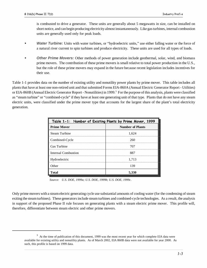
Table 1-1 provides data on the number of existing utility and nonutility power plants by prime mover. This table includes allplants that have at least one non-retired unit and that submitted Forms EIA-860A (Annual Electric Generator Report - Utilities)or EIA-860B (Annual Electric Generator Report - Nonutilities) in 1999.3 For the purpose of this analysis, plants were classifiedas “steam turbine” or “combined-cycle” if they have at least one generating unit of that type. Plants that do not have any steamelectric units, were classified under the prime mover type that accounts for the largest share of the plant’s total electricitygeneration.
Table 1-1: Number of Existing Plants by Prime Mover, 1999
Prime Mover Number of Plants
Steam Turbine 1,624
Combined-Cycle 260
Gas Turbine 707
Internal Combustion 887
Hydroelectric 1,713
Other 139
Total 5,330
Source: U.S. DOE, 1999a; U.S. DOE, 1999b; U.S. DOE, 1999c.
Only prime movers with a steam electric generating cycle use substantial amounts of cooling water (for the condensing of steamexiting the steam turbines). These generators include steam turbines and combined-cycle technologies. As a result, the analysisin support of the proposed Phase II rule focuses on generating plants with a steam electric prime mover. This profile will,therefore, differentiate between steam electric and other prime movers.

§ 316(b) Phase II TDD Industry Profile
4 The numbers presented in this section are capability for utility facilities and capacity for nonutilities. Forconvenience purposes, this section will refer to both measures as“capacity.”
5 More accurate data were available starting in 1991, therefore, 1991 was selected as the initial year for trendsanalysis.
1-4
1-2 DOMESTIC PRODUCTION
This section presents an overview of U.S. generating capacity and electricity generation. Subsection 1-2.1 provides data oncapacity, and Subsection 1-2.2 provides data on generation. Subsection 1-2.3 presents an overview of the geographicdistribution of generation plants and capacity.
1-2.1 Generating Capacity4
The rating of a generating unit is a measure of its ability to produce electricity. Generator ratings are expressed in megawatts(MW). Capacity and capability are the two common measures (U.S. DOE, 2000a):
Nameplate capacity is the full-load continuous output rating of the generating unit under specified conditions, as designatedby the manufacturer.
Net capability is the steady hourly output that the generating unit is expected to supply to the system load, as demonstratedby test procedures. The capability of the generating unit in the summer is generally less than in the winter due to highambient-air and cooling-water temperatures, which cause generating units to be less efficient. The nameplate capacity of agenerating unit is generally greater than its net capability.
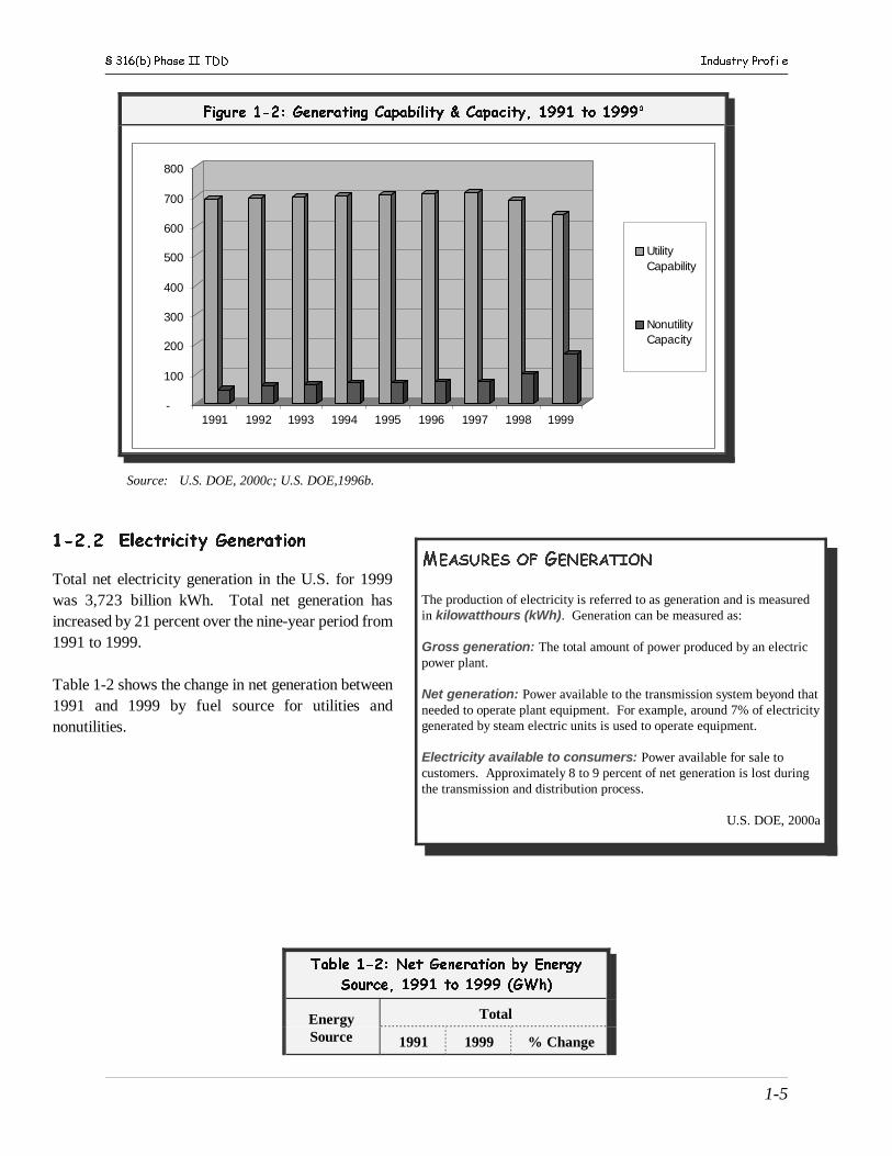
Figure 1-2 shows the total US generating capacity from 1991 to 1999.5
§ 316(b) Phase II TDD Industry Profile
1-5
-
100
200
300
400
500
600
700
800
1991 1992 1993 1994 1995 1996 1997 1998 1999
UtilityCapability
NonutilityCapacity
Figure 1-2: Generating Capability & Capacity, 1991 to 1999a
Source: U.S. DOE, 2000c; U.S. DOE,1996b.
1-2.2 Electricity Generation
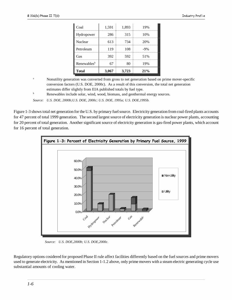
Total net electricity generation in the U.S. for 1999was 3,723 billion kWh. Total net generation hasincreased by 21 percent over the nine-year period from1991 to 1999.
Table 1-2 shows the change in net generation between1991 and 1999 by fuel source for utilities andnonutilities.
Table 1-2: Net Generation by Energy
Source, 1991 to 1999 (GWh)
EnergySource
Total
1991 1999 % Change
MEASURES OF GENERATION
The production of electricity is referred to as generation and is measuredin kilowatthours (kWh). Generation can be measured as:
Gross generation: The total amount of power produced by an electricpower plant.
Net generation: Power available to the transmission system beyond thatneeded to operate plant equipment. For example, around 7% of electricitygenerated by steam electric units is used to operate equipment.
Electricity available to consumers: Power available for sale tocustomers. Approximately 8 to 9 percent of net generation is lost duringthe transmission and distribution process.
U.S. DOE, 2000a
§ 316(b) Phase II TDD Industry Profile
1-6
0.0%
10.0%
20.0%
30.0%
40.0%
50.0%
60.0%
Coal
Hydro
power
Nuclea
r
Petrole
um Gas
Renew
ables
Non-Utility
Utility
Coal 1,591 1,893 19%
Hydropower 286 315 10%
Nuclear 613 734 20%
Petroleum 119 108 -9%
Gas 392 592 51%
Renewablesb 67 80 19%
Total 3,067 3,723 21%
a Nonutility generation was converted from gross to net generation based on prime mover-specificconversion factors (U.S. DOE, 2000c). As a result of this conversion, the total net generationestimates differ slightly from EIA published totals by fuel type.
b Renewables include solar, wind, wood, biomass, and geothermal energy sources.
Source: U.S. DOE, 2000b;U.S. DOE, 2000c; U.S. DOE, 1995a; U.S. DOE,1995b.
Figure 1-3 shows total net generation for the U.S. by primary fuel source. Electricity generation from coal-fired plants accountsfor 47 percent of total 1999 generation. The second largest source of electricity generation is nuclear power plants, accountingfor 20 percent of total generation. Another significant source of electricity generation is gas-fired power plants, which accountfor 16 percent of total generation.
Figure 1-3: Percent of Electricity Generation by Primary Fuel Source, 1999
Source: U.S. DOE,2000b; U.S. DOE,2000c.
Regulatory options cosidered for proposed Phase II rule affect facilities differently based on the fuel sources and prime moversused to generate electricity. As mentioned in Section 1-1.2 above, only prime movers with a steam electric generating cycle usesubstantial amounts of cooling water.
§ 316(b) Phase II TDD Industry Profile
6 EPA applied sample weights to the 539 facilities to account for non-sampled facilities and facilities that did notrespond to the survey. For more information on EPA’s 2000 Section 316(b) Industry Survey, please refer to the InformationCollection Request (U.S. EPA 2000).
1-7
1-3 EXISTING PLANTS WITH CWIS AND NPDES PERMITS
Section 316(b) of the Clean Water Act applies to a point source facility that uses or proposes to use a cooling water intakestructure water that directly withdraws cooling water from a water of the United States. Among power plants, only thosefacilities employing a steam electric generating technology require cooling water and are therefore of interest to this analysis.Steam electric generating technologies include units with steam electric turbines and combined-cycle units with a steamcomponent.
The following sections describe existing power plants that would be subject to the proposed Phase II rule. The Proposed Section316(b) Phase II Existing Facilities Rule applies to existing steam electric power generating facilities that meet all of thefollowing conditions:
< They meet the definition of an existing steam electric power generating facility as specified in § 125.93 of thisrule;
< They use a cooling water intake structure or structures, or obtain cooling water by any sort of contract orarrangement with an independent supplier who has a cooling water intake structure;
< Their cooling water intake structure(s) withdraw(s)cooling water from waters of the U.S., and at leasttwenty-five (25) percent of the water withdrawn isused for contact or non-contact cooling purposes;
< They have an NPDES permit or are required toobtain one; and
< They have a design intake flow of 50 MGD orgreater.
The proposed Phase II rule also covers substantial additions ormodifications to operations undertaken at such facilities. While allfacilities that meet these criteria are subject to the regulation, thisdocument focuses on 539 steam electric power generating facilitiesidentified in EPA’s 2000 Section 316(b) Industry Survey as being“in-scope” of this proposed rule. These 539 facilities represent 550facilities nation-wide.6 The remainder of this chapter will refer tothese facilities as “existing section 316(b) plants.”
Utilities and nonutilities are discussed in separate subsections becausethe data sources, definitions, and potential factors influencing themagnitude of impacts are different for the two sectors. Eachsubsection presents the following information:
< Plant size: This section discusses the existingsection 316(b) facilities by the size of theirgeneration capacity. The size of a plant is important
WATER USE BY STEAM ELECTRIC
POWER PLANTS
Steam electric generating plants are the singlelargest industrial users of water in the United States. In 1995:
< steam electric plants withdrew an estimated190 billion gallons per day, accounting for 39percent of freshwater use and 47 percent ofcombined fresh and saline water withdrawalsfor offstream uses (uses that temporarily orpermanently remove water from its source);
< fossil-fuel steam plants accounted for 71percent of the total water use by the powerindustry;
< nuclear steam plants and geothermal plantsaccounted for 29 percent and less than 1percent, respectively;
< surface water was the source for more than 99percent of total power industry withdrawals;
< approximately 69 percent of water intake bythe power industry was from freshwatersources, 31 percent was from saline sources.
USGS, 1995

§ 316(b) Phase II TDD Industry Profile
7 Once-through cooling systems withdraw water from the water body, run the water through condensers, anddischarge the water after a single use. Recirculating systems, on the other hand, reuse water withdrawn from the source. These systems take new water into the system only to replenish losses from evaporation or other processes during the coolingprocess. Recirculating systems use cooling towers or ponds to cool water before passing it through condensers again.
1-8
because it partly determines its need for cooling water.
< Geographic distribution: This section discusses plants by NERC region. The geographic distribution offacilities is important because a high concentration of facilities with costs under a regulation could lead toimpacts on a regional level. Everything else being equal, the higher the share of plants with costs, the higherthe likelihood that there may be economic and/or system reliability impacts as a result of the regulation.
< Water body and cooling system type: This section presents information on the type of water body from whichexisting section 316(b) facilities draw their cooling water and the type of cooling system they operate. Coolingsystems can be either once-through or recirculating systems.7 Plants with once-through cooling water systemswithdraw between 70 and 98 percent more water than those with recirculating systems.
§ 316(b) Phase II TDD Industry Profile
8 U.S. DOE, 1999a (Annual Electric Generator Report) collects data used to create an annual inventory of utilities. The data collected includes: type of prime mover; nameplate rating; energy source; year of initial commercial operation;operating status; cooling water source, and NERC region.
1-9
1-3.1 Existing Section 316(b) Utility Plants
EPA identified steam electric prime movers that require cooling water using information from the EIA data collection U.S. DOE,1999a.8 These prime movers include:
< Atmospheric Fluidized Bed Combustion (AB)< Combined-Cycle Steam Turbine with Supplementary Firing (CA)< Combined Cycle - Total Unit (CC)< Steam Turbine – Common Header (CH)< Combined-Cycle – Single Shaft (CS)< Combined-Cycle Steam Turbine – Waste Heat Boiler Only (CW)< Steam Turbine – Geothermal (GE)< Integrated Coal Gasification Combined-Cycle (IG)< Steam Turbine – Boiling Water Nuclear Reactor (NB)< Steam Turbine – Graphite Nuclear Reactor (NG)< Steam Turbine – High Temperature Gas-Cooled Nuclear Reactor (NH)< Steam Turbine – Pressurized Water Nuclear Reactor (NP)< Steam Turbine – Solar (SS)< Steam Turbine – Boiler (ST)
Using this list of steam electric prime movers, and U.S. DOE, 1999a information on the reported operating status of units, EPAidentified 862 facilities that have at least one generating unit with a steam electric prime mover. Additional information fromthe section 316(b) Industry Surveys was used to determine that 416 of the 862 facilities operate a CWIS and hold an NPDESpermit. Table 1-4 provides information on the number of utilities, utility plants, and generating units, and the generatingcapacity in 1999. The table provides information for the industry as a whole, for the steam electric part of the industry, andfor the part of the industry potentially affected by the proposed Phase II rule.
Table 1-4: Number of Existing Utilities, Utility Plants, Units, and Capacity, 1999
TotalaSteam Electricb Steam Electric with CWIS
and NPDES Permitc
Number % of Total Number % of Total
Utilities 891 315 35% 148 17%
Plants 3,125 862 28% 416 13%
Units 10,460 2,226 21% 1,220 12%
Nameplate Capacity (MW) 702,624 533,503 76% 344,849 49%
a Includes only generating capacity not permanently shut down or sold to nonutilities.b Utilities and plants are listed as steam electric if they have at least one steam electric unit.c The number of plants, units, and capacity was sample weighted to account for survey non-
respondents.
§ 316(b) Phase II TDD Industry Profile
1-10
189
91
61
3524
104 2 0
0
20
40
60
80
100
120
140
160
180
200
< 50
0
500 -
1,0
00
1,00
0 - 1
,500
1,50
0 - 2
,000
2.00
0 - 2
,500
2,50
0 - 3
,000
3,00
0 - 3
,500
3,50
0 - 4
,000
> 4,0
01
Number ofPlants
Source: U.S. EPA, 2000; U.S. DOE, 1999a; U.S. DOE, 1999c.
Table 1-4 shows that the while the 862 steam electric plants account for only 28 percent of all plants, these plants account for76 percent of all capacity. The 416 in-scope plants represent 13 percent of all plants, are owned by 17 percent of all utilities,and account for approximately 49 percent of reported utility generation capacity. The remainder of this section will focus onthe 416 utility plants.
a. Plant size
EPA analyzed the utility steam electric facilities with a CWIS and an NPDES permit with respect to their generating capacity. Figure 1-4 presents the distribution of existing utility plants with a CWIS and an NPDES permit by plant size. Of the 416plants, 189 (45 percent) have a total nameplate capacity of 500 megawatts or less, and 280 (67 percent) have a total capacityof 1,000 megawatts or less.
Figure 1-4: Number of Existing Phase II Facilities by Plant Size (in MW), 1999 a,b
a Numbers may not add up to totals due to independent rounding.b The number of plants was sample weighted to account for survey non-respondents.
Source: U.S. EPA, 2000; U.S. DOE, 1999a; U.S. DOE, 1999c.
b. Geographic distribution
Table 1-5 shows the distribution of existing section 316(b) utility plants by NERC region. The table shows that there areconsiderable differences between the regions in terms of both the number of existing utility plants with a CWIS and an NPDESpermit, and the percentage of all plants that they represent. Excluding Alaska, which only has one utility plant with a CWISand an NPDES permit, the percentage of existing section 316(b) facilities ranges from two percent in the Western SystemsCoordinating Council (WSCC) to 49 percent in the Electric Reliability Council of Texas (ERCOT). The Southeastern ElectricReliability Council (SERC) has the highest absolute number of existing section 316(b) facilities with 94, or 23 percent of all
§ 316(b) Phase II TDD Industry Profile
1-11
facilities, followed by the East Central Area Reliability Coordination Agreement (ECAR) with 90 facilities, or 22 percent ofall facilities.
Table 1-5: Existing Utility Plants by NERC Region, 1999
NERC RegionTotal Number of
Plants
Plants with CWIS and NPDES Permita,b
Number % of Total
ASCC 168 1 1%
ECAR 301 90 30%
ERCOT 107 52 49%
FRCC 62 29 47%
HI 16 3 19%
MAAC 93 3 3%
MAIN 207 33 16%
MAPP 406 43 11%
NPCC 394 17 4%
SERC 333 94 28%
SPP 262 32 12%
WSCC 773 18 2%
Unknown 3 0 0%
Total 3,125 416 13%
a Numbers may not add up to totals due to independent rounding.b The number of plants was sample weighted to account for survey non-respondents.
Source: U.S. EPA, 2000; U.S. DOE, 1999a; U.S. DOE, 1999c.
§ 316(b) Phase II TDD Industry Profile
9 U.S. DOE, 1998b (Annual Nonutility Electric Generator Report) is the equivalent of U.S. DOE, 1998a for utilities. It is the annual inventory of nonutility plants and collects data on the type of prime mover, nameplate rating, energy source,year of initial commercial operation, and operating status.
1-12
c. Water body and cooling system type
Table 1-6 shows that most of the existing utility plants with a CWIS and an NPDES permit draw water from a freshwater river(204, or 49 percent). The next most frequent water body types are lakes or reservoirs with 138 plants (33 percent) and estuariesor tidal rivers with 47 plants (11 percent). The table also shows that most of these plants, 314 or 75 percent, employ a once-through cooling system. Of the plants that withdraw from an estuary, the most sensitive type of water body, only nine percentuse a recirculating system while 85 percent have a once-through system.
Table 1-6: Number of Existing Utility Plants by Water Body Type and Cooling System Typea
Water BodyType
Cooling System Type
Recirculating Once-Through Combination Other Unknown
Total b
No.% ofTotal
No.% ofTotal
No.% ofTotal
No.% ofTotal
No.% ofTotal
Estuary/Tidal River
4 9% 40 85% 1 2% 2 4% 0 0% 47
Ocean 0 0% 15 100% 0 0% 0 0% 0 0% 15
Lake/Reservoir
29 21% 103 75% 4 3% 2 1% 0 0% 138
FreshwaterRiver
36 18% 149 73% 8 4% 10 5% 1 0% 204
MultipleFreshwater
0 0% 6 60% 3 30% 1 10% 0 0% 10
Other/Unknown
1 50% 1 50% 0 0% 0 0% 0 0% 2
Total 70 17% 314 75% 16 4% 15 4% 1 0% 416
a The number of plants was sample weighted to account for survey non-respondents.b Numbers may not add up to totals due to independent rounding.
Source: U.S. EPA, 2000; U.S. DOE, 1999a; U.S. DOE, 1999c.
1-3.2 Existing Section 316(b) Nonutility Plants
EPA identified nonutility steam electric prime movers that require cooling water using information from the EIA data collectionForms EIA-860B9 and the section 316(b) Industry Survey. These prime movers include:
< Geothermal Binary (GB)< Steam Turbine – Fluidized Bed Combustion (SF)< Solar – Photovoltaic (SO)
§ 316(b) Phase II TDD Industry Profile
1-13
< Steam Turbine (ST)
In addition, prime movers that are part of a combined-cycle unit were classified as steam electric.
U.S. DOE, 1998b includes two types of nonutilities: facilities whose primary business activity is the generation of electricity,and manufacturing facilities that operate industrial boilers in addition to their primary manufacturing processes. The discussionof existing section 316(b) nonutilities focuses on those nonutility facilities that generate electricity as their primary line ofbusiness.
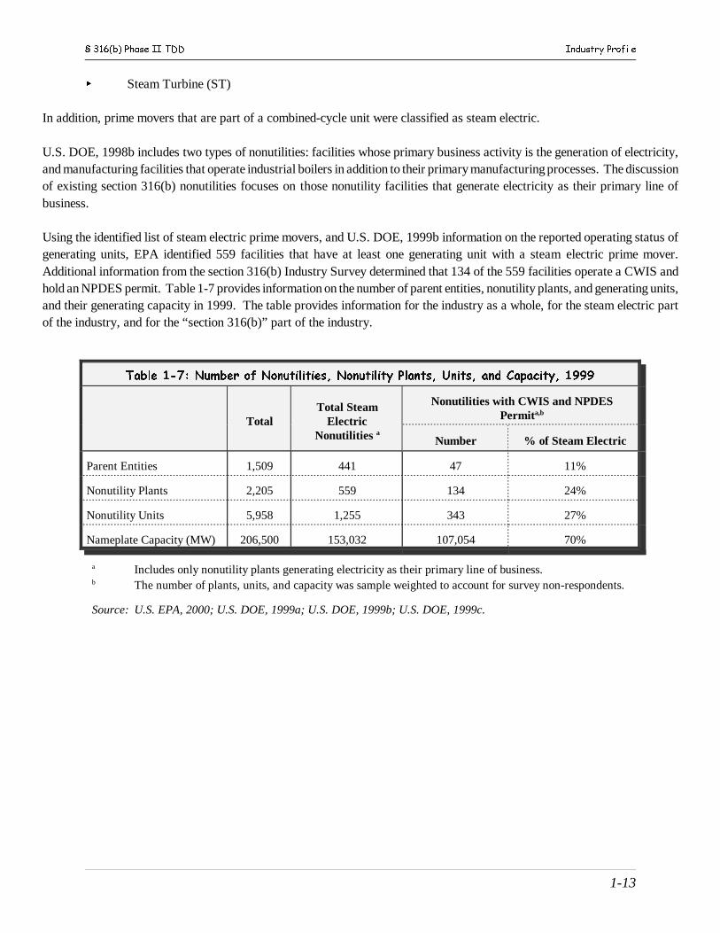
Using the identified list of steam electric prime movers, and U.S. DOE, 1999b information on the reported operating status ofgenerating units, EPA identified 559 facilities that have at least one generating unit with a steam electric prime mover.Additional information from the section 316(b) Industry Survey determined that 134 of the 559 facilities operate a CWIS andhold an NPDES permit. Table 1-7 provides information on the number of parent entities, nonutility plants, and generating units,and their generating capacity in 1999. The table provides information for the industry as a whole, for the steam electric partof the industry, and for the “section 316(b)” part of the industry.
Table 1-7: Number of Nonutilities, Nonutility Plants, Units, and Capacity, 1999
TotalTotal Steam
ElectricNonutilities a
Nonutilities with CWIS and NPDESPermita,b
Number % of Steam Electric
Parent Entities 1,509 441 47 11%
Nonutility Plants 2,205 559 134 24%
Nonutility Units 5,958 1,255 343 27%
Nameplate Capacity (MW) 206,500 153,032 107,054 70%
a Includes only nonutility plants generating electricity as their primary line of business.b The number of plants, units, and capacity was sample weighted to account for survey non-respondents.
Source: U.S. EPA, 2000; U.S. DOE, 1999a; U.S. DOE, 1999b; U.S. DOE, 1999c.
§ 316(b) Phase II TDD Industry Profile
1-14
-
36 5
12
5
20
1
38
-
44
--
5
10
15
20
25
30
35
40
45
< 50
50 -
100
100
- 250
250
- 500
500
- 1,00
0
>1,00
0
Former Utilities
OriginalNonutilities
0 0 0
a. Plant size
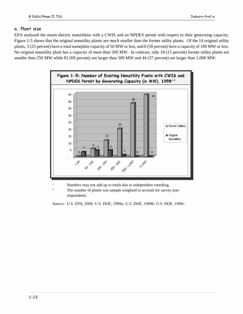
EPA analyzed the steam electric nonutilities with a CWIS and an NPDES permit with respect to their generating capacity.Figure 1-5 shows that the original nonutility plants are much smaller than the former utility plants. Of the 14 original utilityplants, 3 (25 percent) have a total nameplate capacity of 50 MW or less, and 8 (58 percent) have a capacity of 100 MW or less.No original nonutility plant has a capacity of more than 500 MW. In contrast, only 18 (15 percent) former utility plants aresmaller than 250 MW while 83 (69 percent) are larger than 500 MW and 44 (37 percent) are larger than 1,000 MW.
Figure 1-5: Number of Existing Nonutility Plants with CWIS and
NPDES Permit by Generating Capacity (in MW), 1998a,b
a Numbers may not add up to totals due to independent rounding.a The number of plants was sample weighted to account for survey non-
respondents.
Source: U.S. EPA, 2000; U.S. DOE, 1999a; U.S. DOE, 1999b; U.S. DOE, 1999c.
§ 316(b) Phase II TDD Industry Profile
10 The total number of plants includes industrial boilers while the number of plants with a CWIS and an NPDESpermit does not. Therefore, the percentages are likely higher than presented.
1-15
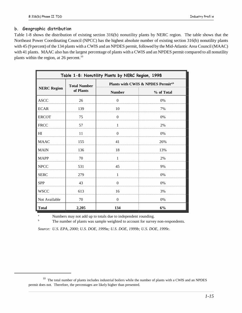
b. Geographic distribution
Table 1-8 shows the distribution of existing section 316(b) nonutility plants by NERC region. The table shows that theNortheast Power Coordinating Council (NPCC) has the highest absolute number of existing section 316(b) nonutility plantswith 45 (9 percent) of the 134 plants with a CWIS and an NPDES permit, followed by the Mid-Atlantic Area Council (MAAC)with 41 plants. MAAC also has the largest percentage of plants with a CWIS and an NPDES permit compared to all nonutilityplants within the region, at 26 percent.10
Table 1-8: Nonutility Plants by NERC Region, 1998
NERC RegionTotal Number
of Plants
Plants with CWIS & NPDES Permita,b
Number % of Total
ASCC 26 0 0%
ECAR 139 10 7%
ERCOT 75 0 0%
FRCC 57 1 2%
HI 11 0 0%
MAAC 155 41 26%
MAIN 136 18 13%
MAPP 70 1 2%
NPCC 531 45 9%
SERC 279 1 0%
SPP 43 0 0%
WSCC 613 16 3%
Not Available 70 0 0%
Total 2,205 134 6%
a Numbers may not add up to totals due to independent rounding.b The number of plants was sample weighted to account for survey non-respondents.
Source: U.S. EPA, 2000; U.S. DOE, 1999a; U.S. DOE, 1999b; U.S. DOE, 1999c.
§ 316(b) Phase II TDD Industry Profile
1-16
c. Water body and cooling system type
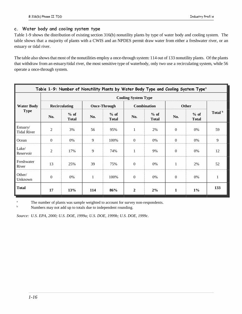
Table 1-9 shows the distribution of existing section 316(b) nonutility plants by type of water body and cooling system. Thetable shows that a majority of plants with a CWIS and an NPDES permit draw water from either a freshwater river, or anestuary or tidal river.
The table also shows that most of the nonutilities employ a once-through system: 114 out of 133 nonutility plants. Of the plantsthat withdraw from an estuary/tidal river, the most sensitive type of waterbody, only two use a recirculating system, while 56operate a once-through system.
Table 1-9: Number of Nonutility Plants by Water Body Type and Cooling System Typea
Water BodyType
Cooling System Type
Recirculating Once-Through Combination Other
Total b
No.% ofTotal
No.% ofTotal
No.% ofTotal
No.% ofTotal
Estuary/Tidal River
2 3% 56 95% 1 2% 0 0% 59
Ocean 0 0% 9 100% 0 0% 0 0% 9
Lake/Reservoir
2 17% 9 74% 1 9% 0 0% 12
FreshwaterRiver
13 25% 39 75% 0 0% 1 2% 52
Other/Unknown
0 0% 1 100% 0 0% 0 0% 1
Total17 13% 114 86% 2 2% 1 1%
133
a The number of plants was sample weighted to account for survey non-respondents.b Numbers may not add up to totals due to independent rounding.
Source: U.S. EPA, 2000; U.S. DOE, 1999a; U.S. DOE, 1999b; U.S. DOE, 1999c.

§ 316(b) Phase II TDD Industry Profile
1-17
1-3.3 Cooling Water Intake Structure Data
A primary source of information used to prepare the analyses of this document is the 316(b) survey. The 316(b) survey wasa two phase process. The results from the second phase of this process -- the distribution of questionnaires to utility andnonutility power producers -- is of specific interest to the analyses in this document. The results from following questionnairesare of interest to this proposed rule: (1) Detailed Industry Questionnaire: Phase II Cooling Water Intake Structures -TraditionalSteam Electric Utilities, (2) Short Technical Industry Questionnaire: Phase II Cooling Water Intake Structures - TraditionalSteam Electric Utilities, (3) Detailed Industry Questionnaire: Phase II Cooling Water Intake Structures - Steam ElectricNonutility Power Producers, and (4) Short Technical Industry Questionnaire: Phase II Cooling Water Intake Structures - SteamElectric Nonutility Power Producers. For the purposes of this document, the results of the detailed industry questionnaires forboth utilities and nonutilities are addressed as simply the detailed questionnaire (the “DQ”) results. Similarly, this documentrefers to the results from the short technical industry questionnaire for both utilities and nonutilities as simply the short technicalquestionnaire (the “STQ”) results. Specific details about the questions may be found in EPA's Information Collection Request(DCN 3-3084-R2 in Docket W-00-03) and in the questionnaires (see DCN 3-0030 and 3-0031 in Docket W-00-03 and Docketfor today’s proposal); these documents are also available on EPA's web site (http://www.epa.gov/waterscience/316b/question/).
All utilities and a sample of nonutility facilities (those identified as in-scope by the results of a screener questionnaire) weresent either a STQ or a DQ. A total of 878 utility facilities and 343 nonutility facilities received one of the two questionnaires.EPA selected a random sample of these eligible facilities to receive a DQ. The sample included 282 utility facilities and 181nonutility facilities. Those facilities not selected to receive a DQ were sent a STQ. More detail is provided in a report,Statistical Summary for Cooling Water Intakes Structures Surveys (See DCN 3-3077 in Docket W-00-03). Of the 282 utilityfacilities and 181 nonutility facilities receiving a DQ, the Agency determined that 225 of the respondents would fall within thescope of this rule. Of the STQ respondents, the Agency found that 314 would be in-scope.
The Agency compiled facility level, cooling system, and intake structure data for the 225 in-scope Detailed Questionnaire (DQ)respondents and, to the extent possible, for the 314 Short Technical Questionnaire (STQ) respondents. The Agency then usedthis tabulation of data to make determinations on the types of cooling systems and intake structures in-place at the in-scopefacilities. The Agency utilized questions about intake systems common to both the DQ and STQ in order to make determinationsabout costing decisions that hinged on the intake structures in-place. Other pieces of information from the STQ provided insightinto the types of intake structures in-place at the STQ facilities, when compared to more detailed information for the DQrespondents.
Using both the DQ and STQ responses, the Agency studied the intake structure characteristics for all 539 facilities and/or the225 DQ facilities. The Agency focused on questions about intake screen structure types common to both the DQ and STQ.The Agency then examined the DQ respondents within the context of these questions to discern patterns and statistics for usein making decisions relating to costing of the proposed option based on intake systems currently in-place for both the DQ andSTQ facilities. Tables 1-10 through 1-19 summarize this data analysis. For discussion and descriptions of the types of coolingwater intake technologies presented in the tables, see Chapter 3 of this document.
§ 316(b) Phase II TDD Industry Profile
1-18
Table 1-10 presents information for the in-scope, DQ respondents relating to the general configuration of their cooling waterintake system, water body from which they withdraw cooling water, and cooling system type. The table also shows that themedian intake velocity for all in-scope, DQ intakes is 1.5 feet per second. Of interest is the fact that of all in-scope DQrespondents, 89 percent of the intakes operate traveling screens and 25 percent report some form of impingement or entrainmentreducing configuration.
Table 1-10 Statistics for all Detailed Questionnaire, In-scope Facilities
Percent Cooling Water Intake Technology
22 cooling tower (recirculating or helper)
36 intake canal or channel
10 embayment/bay/cove
30 submerged shoreline intake
38 surface shoreline intake
14 submerged offshore intake
95 trash racks
97 intake screen
25 impingement / entrainment technology
5 passive intake
6 fish diversion or avoidance
32 fish handling and/or return
89 traveling screens
Percent Cooling System Type
76 once-through
12 recirculating cooling
11 combination cooling
1 other cooling type
Percent Intake Velocity (median intake velocity = 1.5 ft/sec)
14 velocity < or = 0.5 fps
Percent Waterbody Type
22 Estuary/Tidal River
5 Ocean
49 Freshwater Stream/River
19 Lake/Reservoir
5 Great Lake
§ 316(b) Phase II TDD Industry Profile
1-19
Table 1-11 shows similar information as in Table 1-10, however, the data is specific to the in-scope respondents to the DQ thatreported impingement/ entrainment technologies. The cooling water intake technology information in the first portion of Table1-11 resembles that of Table 1-10. However, the percentage of intakes with fish handling / fish return technologies isconsiderably higher for those reporting impingement / entrainment technologies compared to all in-scope DQ intakes. Thedistribution of cooling system types are similar for Tables 1-10 and 1-11, as is the median velocity.
Table 1-11 Statistics for DQ Intakes with Impingement / Entrainment Technologies
Percent Cooling Water Intake Technology
22 cooling tower (recirculating or helper)
34 intake canal or channel
7 embayment/bay/cove
34 submerged shoreline intake
37 surface shoreline intake
5 submerged offshore intake
94 trash racks
98 intake screen
8 passive intake
2 fish diversion or avoidance
59 fish handling and/or return
Percent Cooling System Type
80 once-through
14 recirculating cooling
5 combination cooling
1 other cooling type
Percent Intake Velocity (median intake velocity = 1.4 ft/sec)
18 velocity < or = 0.5 fps
Percent Waterbody Type
41 Estuary/Tidal River
4 Ocean
35 Freshwater Stream/River
19 Lake/Reservoir
2 Great Lake
§ 316(b) Phase II TDD Industry Profile
1-20
Table 1-12 presents the number and capacity of the intakes for the in-scope DQ respondents. Key statistics, in the Agency’sview, are the number of intakes per facility (less than two), the distribution of the number of intakes at in-scope DQ respondentfacilities (64 percent with only one intake and only 11 percent of facilities with three or more intakes), and the average percentof intake flow used for cooling (86 percent).
Table 1-12. Number and Capacity of Intakes for In-Scope Detailed Questionnaire Facilities
Characteristic Value
median design capacity per intake (gpd) for all intakes 219,000,000
median design capacity per facility (gpd) for all facilities 374,000,000
median capacity per intake (gpd) for facilities at or below median facility flow 100,800,000
median capacity per intake (gpd) for facilities above median facility flow 408,400,000
average number of intakes per facility for all facilities 1.6
Facilities with only 1 intake 64 %
Facilities with 2 or more intakes 36 %
Facilities with 3 or more intakes 11 %
Facilities at or below median facility flow with 2 or more intakes 26 %
Facilities above median facility flow with 2 or more intakes 46 %
Facilities at or below median facility flow with 3 or more intakes 4 %
Facilities above median facility flow with 3 or more intakes 17 %
Facilities at or below median facility flow with 4 or more intakes 1 %
Facilities above median facility flow with 4 or more intakes 8 %
Facilities with four or more intakes 4 %
Average number of intakes per facility at or below median facility flow 1.3
Average number of intakes per facility above median facility flow 1.8
Average percent of intake used for cooling per intake (all facilities) 86 %
Average percent of intake used for cooling for facilities at or below median flow 86 %
Average percent of intake used for cooling for facilities above median facility flow 87 %
§ 316(b) Phase II TDD Industry Profile
1-21
Table 1-13 gives a breakdown of the type of fish handling / return systems at in-scope DQ facilities. Table 1-14 presents thesame information, but only for the in-scope DQ respondents that reported both fish handling / fish return systems andimpingement/ entrainment reducing configurations. Clearly, the most prevalent form of fish handling / return system is theconveyance system. See Chapter 3 of this document for descriptions of the types of fish handling / return systems.
Table 1-13. Statistics for DQ Facilities Reporting Fish Handling/Return Systems
Percent Characteristic
8 fish pump
94 fish conveyance system
4 fish elevator/lift baskets
3 fish bypass
1 fish holding tank
3 other handling/return system
10 more than one of the above
Table 1-14. Statistics for Facilities Reporting Fish Handling / Returns
AND Impingement / Entrainment Systems in Detailed Quetionnaire
Percent Characteristic
14 fish pump
86 fish conveyance system
8 fish elevator/lift baskets
6 fish bypass
2 fish holding tank
6 other handling/return system
18 more than one of the above
§ 316(b) Phase II TDD Industry Profile
1-22
Table 1-15 presents information for the in-scope DQ respondents that reported shoreline intakes (either surface or submergedintakes). Interestingly, the median surface water depth for surface and submerged shoreline intakes is very similar(approximately 18 feet). The percentage of in-scope DQ respondents with shoreline intakes is split, roughly equally, betweensubmerged and surface configurations. The majority (77 percent) of all shoreline intakes are flush with the shore and only 8percent protrude offshore.
Table 1-15. Statistics for Detailed Questionnaire Shoreline Intakes
characteristic value
median surface water depth for both submerged and surface intakes (ft) 18
median surface water depth for surface intakes (ft) 17
median surface water depth for submerged intakes (ft) 18
median distance from top of intake to surface for all shoreline intakes (ft) 9
median distance from intake bottom to surface for all shoreline intakes (ft) 18
Percent of all shoreline intakes submerged 45
Percent of all shoreline intakes surface 55
Percent of all shoreline intakes flush with shore 77
Percent of all shoreline intakes recessed 15
Percent of all shoreline intakes protruding offshore 8
Percent of all shoreline intakes with skimmer/curtain/baffle wall 45
Tables 1-16 and 1-17 present basic information from the in-scope DQ respondents on the percent of fine-mesh screens andpassive intakes in-place at these facilities. In addition, Table 1-16 includes the Agency’s projection of the total number of fine-mesh screens at STQ respondents (note: the STQ did not collect information of sufficient detail to distinguish fine-mesh fromcoarse-mesh screens).
Table 1-16. Statistics for Fine Mesh Screens
Characteristic Value
Detailed Questionnaire Intakes with Fine Mesh in-place 1.3 %
Detailed Questionniare Estuarine Intakes with Fine Mesh in-place 4.3%
Projected Number of Short Technical Questionnaire Intakes with Fine Mesh in-place 6
Table 1-17. Statistics for Passive Intake
Percent Characteristic
5.4 Percent of All Intakes reported as Passive Intakes
5.3 Percent of Estuarine Intakes reported as Passive
§ 316(b) Phase II TDD Industry Profile
1-23
Table 1-18 presents detailed information from the in-scope DQ respondents with offshore intakes. The percentage ofimpingement / entrainment technologies on offshore intakes is very low (2 percent). The median distance from shore is 450 feetand the median surface water depth is 30 feet at the intake. As expected, ocean intakes show the highest percentage of offshoreconfigurations.
Table 1-18. Statistics for Intakes Reported as Offshore in the Detailed Questionnaire
Characteristic Value
all DQ intakes Offshore 10
% of intakes reporting I/E Offshore 2
Median distance to shore for Offshore intakes (feet) 450
Median surface water depth at Offshore intake (feet) 30
Percent of estuarine intakes Offshore 5
Percent of ocean intakes Offshore 41
Percent of lake / Reservoir intakes Offshore 16
Percent of freshwater stream / river intakes Offshore 11
Percent of Great Lake intakes Offshore 35
Table 1-19 presents information for in-scope DQ intakes reporting canal or channel configurations. The median canal/channellength from mouth to pumps is 1000 feet. The cross-sectional water level ranges from 470 ft (median of reported low-waterlevels) to 620 ft (median of reported mean-water levels).
Table 1-19. Statistics for DQ Intakes Reporting Canal/Channel
Characteristic Value
Median Length Canal Mouth to Pumps (ft) 1000
Median Intake X-Section-Low Water (ft) 472
Median Intake X-Section-Mean Water (ft) 617
Median Distance curtain/baffle from canal mouth (ft) 650
Median intake bay depth (ft) 17
Percent of canal/channel intakes with submerged shoreline Intakes 9 %
Percent of canal/channel intakes with surface shoreline intakes 19 %
Percent of canal/channel intakes with flush intakes 20 %
Percent of canal/channel intakes with recessed intakes 6 %
Percent of canal/channel intakes with protruding intakes 2 %
§ 316(b) Phase II TDD Industry Profile
1-24
GLOSSARY
Baseload: A baseload generating unit is normally used to satisfy all or part of the minimum or base load of the systemand, as a consequence, produces electricity at an essentially constant rate and runs continuously. Baseload units aregenerally the newest, largest, and most efficient of the three types of units.(http://www.eia.doe.gov/cneaf/electricity/page/prim2/chapter2.html)
Combined-Cycle Turbine: An electric generating technology in which electricity is produced from otherwise lost wasteheat exiting from one or more gas (combustion) turbines. The exiting heat is routed to a conventional boiler or to heatrecovery steam generator for utilization by a steam turbine in the production of electricity. This process increases theefficiency of the electric generating unit.
Distribution: The portion of an electric system that is dedicated to delivering electric energy to an end user.
Electricity Available to Consumers: Power available for sale to customers. Approximately 8 to 9 percent of netgeneration is lost during the transmission and distribution process.
Energy Policy Act (EPACT): In 1992 the EPACT removed constraints on ownership of electric generation facilitiesand encouraged increased competition on the wholesale electric power business.
Gas Combustion Turbine: A gas turbine typically consisting of an axial-flow air compressor and one or morecombustion chambers, where liquid or gaseous fuel is burned and the hot gases are passed to the turbine. The hot gasesexpand to drive the generator and are then used to run the compressor.
Generation: The process of producing electric energy by transforming other forms of energy. Generation is also theamount of electric energy produced, expressed in watthours (Wh).
Gross Generation: The total amount of electric energy produced by the generating units at a generating station orstations, measured at the generator terminals.
Intermediate load: Intermediate-load generating units meet system requirements that are greater than baseload but lessthan peakload. Intermediate-load units are used during the transition between baseload and peak load requirements.(http://www.eia.doe.gov/cneaf/electricity/page/prim2/chapter2.html)
Internal Combustion Engine: An internal combustion engine has one or more cylinders in which the process ofcombustion takes place, converting energy released from the rapid burning of a fuel-air mixture into mechanical energy. Diesel or gas-fired engines are the principal fuel types used in these generators.
Kilowatthours (kWh): One thousand watthours (Wh).
Nameplate Capacity: The amount of electric power delivered or required for which a generator, turbine, transformer,transmission circuit, station, or system is rated by the manufacturer.
Net Capacity: The amount of electric power delivered or required for which a generator, turbine, transformer,transmission circuit, station, or system is rated by the manufacturer, exclusive of station use, and unspecified conditions for
§ 316(b) Phase II TDD Industry Profile
1-25
a given time interval.
Net Generation: Gross generation minus plant use from all plants owned by the same utility.
Nonutility: A corporation, person, agency, authority, or other legal entity or instrumentality that owns electric generatingcapacity and is not an electric utility. Nonutility power producers include qualifying cogenerators, qualifying small powerproducers, and other nonutility generators (including independent power producers) without a designated franchised servicearea that do not file forms listed in the Code of Federal Regulations, Title 18, Part 141.(http://www.eia.doe.gov/emeu/iea/glossary.html)
Other Prime Movers: Methods of power generation other than steam turbine, combined-cycle, gascombustion turbine, internal combustion engine, and water turbine. Other prime movers include: geothermal,solar, wind, and biomass.
Peakload: A peakload generating unit, normally the least efficient of the three unit types, is used to meet requirementsduring the periods of greatest, or peak, load on the system.(http://www.eia.doe.gov/cneaf/electricity/page/prim2/chapter2.html)
Power Marketers: Business entities engaged in buying, selling, and marketing electricity. Power marketers do notusually own generating or transmission facilities. Power marketers, as opposed to brokers, take ownership of the electricityand are involved in interstate trade. These entities file with the Federal Energy Regulatory Commission for status as apower marketer. (http://www.eia.doe.gov/cneaf/electricity/epav1/glossary.html)
Power Brokers: An entity that arranges the sale and purchase of electric energy, transmission, and other servicesbetween buyers and sellers, but does not take title to any of the power sold.(http://www.eia.doe.gov/cneaf/electricity/epav1/glossary.html)
Prime Movers: The engine, turbine, water wheel or similar machine that drives an electric generator. Also, for reportingpurposes, a device that directly converts energy to electricity, e.g., photovoltaic, solar, and fuel cell(s).
Public Utility Regulatory Policies Act (PURPA): In 1978 PURPA opened up competition in the electricitygeneration market by creating a class of nonutility electricity-generating companies referred to as “qualifying facilities.”
Reliability: Electric system reliability has two components: adequacy and security. Adequacy is the ability of the electricsystem to supply customers at all times, taking into account scheduled and unscheduled outages of system facilities.Security is the ability of the electric system to withstand sudden disturbances, such as electric short circuits or unanticipatedloss of system facilities. (http://www.eia.doe.gov/cneaf/electricity/epav1/glossary.html)
Steam Turbine: A generating unit in which the prime mover is a steam turbine. The turbines convert thermal energy(steam or hot water) produced by generators or boilers to mechanical energy or shaft torque. This mechanical energy isused to power electric generators, including combined-cycle electric generating units, that convert the mechanical energy toelectricity.
Transmission: The movement or transfer of electric energy over an interconnected group of lines and associatedequipment between points of supply and points at which it is transformed for delivery to consumers, or is delivered to other

§ 316(b) Phase II TDD Industry Profile
1-26
electric systems. Transmission is considered to end when the energy is transformed for distribution to the consumer.
Utility: A corporation, person, agency, authority, or other legal entity or instrumentality that owns and/or operatesfacilities within the United States, its territories, or Puerto Rico for the generation, transmission, distribution, or sale ofelectric energy primarily for use by the public and files forms listed in the Code of Federal Regulations, Title 18, Part 141.Facilities that qualify as cogenerators or small power producers under the Public Utility Regulatory Policies Act (PURPA)are not considered electric utilities. (http://www.eia.doe.gov/emeu/iea/glossary.html)
Water Turbine: A unit in which the turbine generator is driven by falling water.
Watt: The electrical unit of power. The rate of energy transfer equivalent to 1 ampere flowing under the pressure of 1 voltat unity power factor.(Does not appear in text)
Watthour (Wh): An electrical energy unit of measure equal to 1 watt of power supplied to, or take from, an electriccircuit steadily for 1 hour. (Does not appear in text)

§ 316(b) Phase II TDD Industry Profile
1-27
REFERENCES
U.S. Department of Energy (U.S. DOE). 2002. Energy Information Administration (EIA). Status of State Electric IndustryRestructuring Activity as of March 2002. At: http://www.eia.doe.gov/cneaf/electricity/chg_str/regmap.html
U.S. Department of Energy (U.S. DOE). 2001. Energy Information Administration (EIA). Annual Energy Outlook 2002 WithProjections to 2020. DOE/EIA-0383(2002). December 2001.
U.S. Department of Energy (U.S. DOE). 2000a. Energy Information Administration (EIA). Electric Power IndustryOverview. At: http://www.eia.doe.gov/cneaf/electricity/page/prim2/toc2.html.
U.S. Department of Energy (U. S. DOE). 2000b. Energy Information Administration (EIA). Electric Power Annual 1999Volume I. DOE/EIA-0348(99)/1.
U.S. Department of Energy (U. S. DOE). 2000c. Energy Information Administration (EIA). Electric Power Annual 1999Volume II. DOE/EIA-0348(99)/2.
U.S. Department of Energy (U.S. DOE). 1999a. Form EIA-860A (1999). Annual Electric Generator Report – Utility.
U.S. Department of Energy (U.S. DOE). 1999b. Form EIA-860B (1999). Annual Electric Generator Report – Nonutility.
U.S. Department of Energy (U.S. DOE). 1999c. Form EIA-861 (1999). Annual Electric Utility Data.
U.S. Department of Energy (U.S. DOE). 1999d. Form EIA-759 (1999). Monthly Power Plant Report.
U.S. Department of Energy (U.S. DOE). 1998a. Energy Information Administration (EIA). Electric Power Annual 1997Volume I. DOE/EIA-0348(97/1).
U.S. Department of Energy (U.S. DOE). 1998b. Energy Information Administration (EIA). Electric Power Annual 1997Volume II. DOE/EIA-0348(97/1).
U.S. Department of Energy (U.S. DOE). 1998c. Form EIA-861 (1998). Annual Electric Utility Data.
U.S. Department of Energy (U.S. DOE). 1996a. Energy Information Administration (EIA). Electric Power Annual 1995Volume I. DOE/EIA-0348(95)/1.
U.S. Department of Energy (U.S. DOE). 1996b. Energy Information Administration (EIA). Electric Power Annual 1995Volume II. DOE/EIA-0348(95)/2.
U.S. Department of Energy (U. S. DOE). 1996c. Energy Information Administration (EIA). Impacts of Electric PowerIndustry Restructuring on the Coal Industry. At: http://www.eia.doe.gov/cneaf/electricity/chg_str_fuel/html/chapter1.html.
U.S. Department of Energy (U.S. DOE). 1995a. Energy Information Administration (EIA). Electric Power Annual 1994Volume I. DOE/EIA-0348(94/1).

§ 316(b) Phase II TDD Industry Profile
1-28
U.S. Department of Energy (U.S. DOE). 1995b. Energy Information Administration (EIA). Electric Power Annual 1994Volume II. DOE/EIA-0348(94/1).
U.S. Environmental Protection Agency (U.S. EPA). 2000. Section 316(b) Industry Survey. Detailed Industry Questionnaire:Phase II Cooling Water Intake Structures and Industry Short Technical Questionnaire: Phase II Cooling Water IntakeStructures, January, 2000 (OMB Control Number 2040-0213). Industry Screener Questionnaire: Phase I Cooling WaterIntake Structures, January, 1999 (OMB Control Number 2040-0203).
U.S. Geological Survey (USGS). 1995. Estimated Use of Water in the United States in 1995. At: http://water.usgs.gov/watuse/pdf1995/html/.

§ 316(b) Phase II TDD Costing Methodology
2.1
Chapter 2: Costing Methodology for
Model Plants
INTRODUCTION
This chapter presents the methodologies used by the Agency to develop cost estimates at the model plant level for theproposed rule and regulatory options considered. The Agency costs for 539 model plants and these were then used inthe economic analysis to scale to the total universe of in-scope facilities. For the model-plant specific projectedcompliance costs of the proposed rule, see Appendix A of this document. Under the proposed rule, facilities have theoption of conducting a cost test against the compliance costs developed by the Agency for support of the regulatoryrequirements of the rule. The costs presented in Appendix A, and developed based on the methodology presented inthis chapter, would form the basis of the “significantly greater” cost test in the proposed rule.
The term model plant is used frequently throughout this document. The Agency notes that model plants are not actualexisting facilities. Model Plants are statistical representations of existing facilities (or fractions of existing facilities).Therefore, the cost estimates developed for the rule should not be considered to reflect those exactly of a particularexisting facility. However, in the Agency’s view, the national estimates of benefits, compliance costs, and economicimpacts are representative of those expected from the industry as a whole.
2.1 COOLING WATER INTAKE STRUCTURE COSTS
EPA developed distinct sets of intake structure and conduit system costs for existing source model plants expected to(1) upgrade screen systems only, (2) upgrade cooling systems and intake structures, and (3) upgrade cooling systemsonly.
For those plants projected to incur costs of cooling water intake structure upgrades (but not flow-reducing coolingsystem conversions), the Agency estimates that intake fanning/expansion would be necessary for the majority of plantsprojected to install entrainment reducing fine-mesh screens. Therefore, the Agency developed capital costs for thesescenarios that incorporate the costs of expanding/fanning or adding an additional bay to an existing intake structure inorder to upgrade to fine-mesh screens. Because fine-mesh screens have reduced open cross-sectional area whencompared to coarse-mesh screens, the Agency considers the intake expansion/fanning costs to be appropriate in thesecases. Even though there is not a set of velocity-based requirements for this proposal, the Agency projects that themodel plants expected to upgrade their intake screens from coarse to fine-mesh would reduce their through-screenvelocity from the median facility value of 1.5 feet/second to 1.0 feet/second as a result of this technology change. Inpart, in the Agency’s view, the reduced velocity would adopted for the operational requirements of the screens and tobalance the impingement reduction benefits of lower velocities with the physical constraints of velocity reduction forexisting intake structures. The Agency utilized costs developed for fine-mesh screens with a through-screen velocityof 1.0 feet/second to size the intake for the full design, once-through intake flow. The operation and maintenance(O&M) costs of these screens are calculated based on the same principle. These capital and O&M costs for fine-meshscreens were developed for the New Facility 316(b) rule and are utilized for existing facilities with some modifications.The Agency applies a capital cost construction inflation factor (in addition to a “retrofit” factor discussed in section
§ 316(b) Phase II TDD Costing Methodology
2.2
2.6) to account for the expansion/fanning of the intake structure, but does not estimate further O&M costs for this one-time activity. Those plants that additionally would install fish handling/return systems to the upgraded screens incurcapital and operation and maintenance costs developed based on the size of the larger size screens. See Sections 2.1.1and 2.1.2 for the development of the cost estimates for capital and O&M costs for fine-mesh screens.
The Agency developed existing facility construction factors (used in addition to “retrofit” factors discussed in Section2.6) based on the average ratio of intake modification construction costs to costs derived from CWIS equationsdeveloped for New Facility projects. Thus the differences reflect differences in construction costs for nuclear and non-nuclear and differences in CWIS installation capital costs. Table 2-1 presents the construction factors for a variety ofcompliance technologies used as the basis for the costs estimated for this proposal and regulatory options.
Table 2-1 CWIS Technology Flow Sizing and Construction Factors for Existing Facilities
Compliance CoolingSystem Type Plant Type
Flow Used to sizeCooling Water IntakeTechnology
Compliance CoolingWater IntakeTechnology
ConstructionFactor forScenario
Non-Cooling Tower Non-nuclear 100% of Once-throughBaseline Design Intake
Fish Handling None
Non-Cooling Tower Non-nuclear 100% of Once-throughBaseline Design Intake
Fine Mesh Screens 30%*
Non-Cooling Tower Non-nuclear 100% of Once-throughBaseline Design Intake
Fine Mesh Screensw/ Fish Handling
15%*
Non-Cooling Tower Nuclear 100% of Once-throughBaseline Design Intake
Fish Handling None
Non-Cooling Tower Nuclear 100% of Once-throughBaseline Design Intake
Fine Mesh Screens 65%*
Non-Cooling Tower Nuclear 100% of Once-throughBaseline Design Intake
Fine Mesh Screensw/ Fish Handling
30%*
* Existing facility construction factors based on average ratio of intake modification construction costs to costs derivedfrom CWIS equations developed for New Facility projects. Thus the differences reflect differences in constructioncosts for nuclear and non-nuclear and differences in CWIS installation capital costs.
** For cooling sizing of cooling towers and appropriate flow for determining the costs of retrofitted cooling watersystems, see Section 2.2.
Intake modification construction costs are based on the following general framework:
! An increase in screen area of 50% due to conversion from coarse-mesh to fine-mesh.
! Screen size increase will involve demolition of one side of intake and extension in that direction.
! Installation/removal of sheet piling.
! Concrete demolition of one column and one side (cost doubled for nuclear*).
§ 316(b) Phase II TDD Costing Methodology
2.3
! Excavation (cost doubled for nuclear*).
! Additional concrete foundation.
! Additional concrete side and back wall.
! Additional concrete column.
* EPA doubled costs to account for concerns that use of blasting and high-impact equipment may be limited at nuclearfacilities.
Modification construction costs were then increased by the following cost factors:
Item Factor
Mobilization/Demobilization 3 %
Engineering 10 %
Site Work 5 %
Electrical 10 %
Controls 3 %
Contingency 10 %
Allowance 5 %
For those model plants projected to only incur costs of installing fish handling/return systems to existing screens, theAgency developed costs by estimating the size of coarse mesh, 1.5 feet/sec screens. The through-screen velocity of 1.5feet/sec is the median velocity for all 316b survey respondents. The Agency determined that use of this metric to sizethe fish handling/return systems was appropriate for the variety of plants projected to incur their capital and operationand maintenance costs as a result of this proposal. The capital cost estimates used here for installation of the fishhandling/return systems to existing screens were those developed for new facilities, with an additional inflation (or“retrofit”) factor to account for the issues discussed in Section 2.6 below. Section 2.1.1 presents the cost estimatesdeveloped for new facilities for fish handling/return systems.
For the those plants projected to incur costs of cooling system conversions and entrainment-reducing fine-mesh screens,the Agency considered the existing intake structures to be of a size too large for a realistic screen retrofit. Therefore,in these cases, the Agency estimated that one-half of the intake bay(s) would be blocked/closed and the retrofitted fine-mesh intake screens would apply to only one-half of the size of the original intake. The Agency considers this areasonable approach to estimating realistic scenarios where the average plant (as demonstrated in Table 1-12) utilizesmultiple intake bays. In the Agency’s view, the plant, when presented an equal opportunity option, would utilize thepotential cost savings option of installing the fine-mesh screens on only the maximum intake area necessary. For thoseplants also projected to incur costs of the addition of fish handling/return systems, the Agency estimates the system sizebased on this concept of closure/blockage of one-half of the existing intake. The operation and maintenance costs arealso developed using this size of an intake. Therefore, for the case of each of these retrofit activities, the installedcapital costs and operation and maintenance costs of the intake screens and fish handling/return systems areapproximately one-half of those for a full size screen replacement.
§ 316(b) Phase II TDD Costing Methodology
2.4
For those model plants converting their cooling systems from once-through to recirculating systems but not incurringcosts of entrainment-reducing intake screens, the existing intake structures are considered to be operational withoutsignificant modification (as was the case in the example of the conversions discussed in Chapter 4). In turn, the plantswould incur no additional operation and maintenance costs.
The Agency notes that in addition to the intake structure capital costs described above, the capital costs are inflated bythe “retrofit” capital cost factor of 30 percent described in section 2.6, below. Therefore, the Agency views the retrofitcapital costs developed for upgrading intake screens and structures to be appropriate for existing model plants.
2.1.1 Capital and O&M Costs of Intake Structures and Conduit Systems
Installation of traveling screens with fish baskets for New Facilities
Single-entry, single-exit vertical traveling screens (conventional traveling screens) contain a series of wire mesh screenpanels that are mounted end to end on a band to form a vertical loop. As water flows through the panels, debris andfish that are larger than the screen openings are caught on the screen or at the base of each panel in a basket. As thescreen rotates around, each panel in turn reaches a top area where a high-pressure jet spray wash pushes debris andfish from the basket into a trash trough for disposal. As the screen rotates over time, the clean panels move down, backinto the water to screen the intake flow.
Conventional traveling screens can be operated continuously or intermittently. However, when these screens are fittedwith fish baskets (also called modified conventional traveling screens or Ristroph screens), the screens must be operatedcontinuously so that fish that are collected in the fish baskets can be released to a bypass/return using a low pressurespray wash when the basket reaches the top of the screen. Once the fish have been removed, a high pressure jet spraywash is typically used to remove debris from the screen. In recent years, the design of fish baskets has been refined(e.g., deeper baskets, smoother mesh, better balance) to decrease chances of injury and mortality and to better retainfish (i.e., prevent them from flopping out and potentially being injured). Methods used to protect fish include theStabilized Integral Marine Protective Lifting Environment (S.I.M.P.L.E.) developed by Brackett Green and theModified Ristroph design by U.S. Filter.
U.S. Filter’s conventional (through flow) traveling screens are typically manufactured in widths ranging from two feetto at least 14 feet, for channel depths of up to 100 feet, although custom design is possible to fit other dimensions.
Flow
To calculate the flow through a screen panel, the width of the screen panel is multiplied by the water depth and, usingthe desired flow velocities (1 foot per second and 0.5 foot per second), is converted to gallons per minute assuming ascreen efficiency of 50 percent. The calculated flows for selected screen widths, water depths, and well depths arepresented in Tables 2-30 and 2-31. For flows greater than this, a facility would generally install multiple screens oruse a custom design.
Well depth includes the height of the structure above the water line. The well depth can be more than the water depthby a few to tens of feet. The flow velocities used are representative of a flow speed that is generally considered to befish friendly particularly for sensitive species (0.5 fps), and a flow speed that may be more practical for some facilities
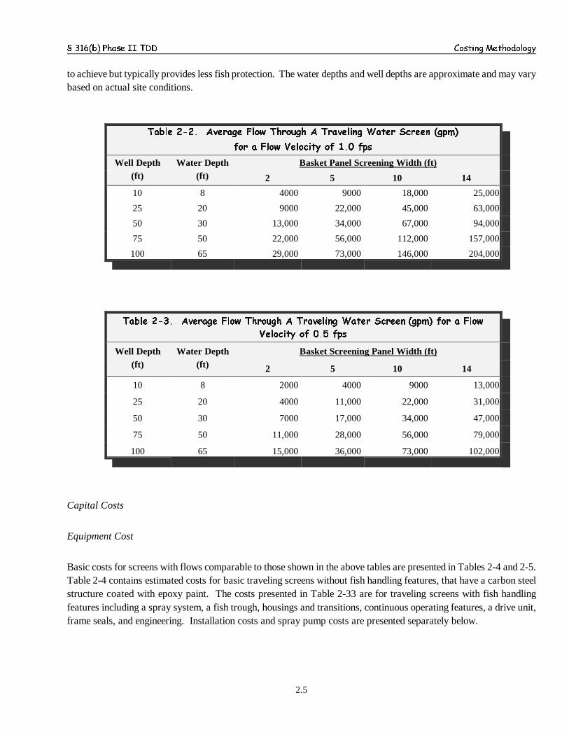
§ 316(b) Phase II TDD Costing Methodology
2.5
to achieve but typically provides less fish protection. The water depths and well depths are approximate and may varybased on actual site conditions.
Table 2-2. Average Flow Through A Traveling Water Screen (gpm)
for a Flow Velocity of 1.0 fps
Well Depth(ft)
Water Depth(ft)
Basket Panel Screening Width (ft)
2 5 10 14
10 8 4000 9000 18,000 25,000
25 20 9000 22,000 45,000 63,000
50 30 13,000 34,000 67,000 94,000
75 50 22,000 56,000 112,000 157,000
100 65 29,000 73,000 146,000 204,000
Table 2-3. Average Flow Through A Traveling Water Screen (gpm) for a Flow
Velocity of 0.5 fps
Well Depth(ft)
Water Depth(ft)
Basket Screening Panel Width (ft)
2 5 10 14
10 8 2000 4000 9000 13,000
25 20 4000 11,000 22,000 31,000
50 30 7000 17,000 34,000 47,000
75 50 11,000 28,000 56,000 79,000
100 65 15,000 36,000 73,000 102,000
Capital Costs
Equipment Cost
Basic costs for screens with flows comparable to those shown in the above tables are presented in Tables 2-4 and 2-5.Table 2-4 contains estimated costs for basic traveling screens without fish handling features, that have a carbon steelstructure coated with epoxy paint. The costs presented in Table 2-33 are for traveling screens with fish handlingfeatures including a spray system, a fish trough, housings and transitions, continuous operating features, a drive unit,frame seals, and engineering. Installation costs and spray pump costs are presented separately below.
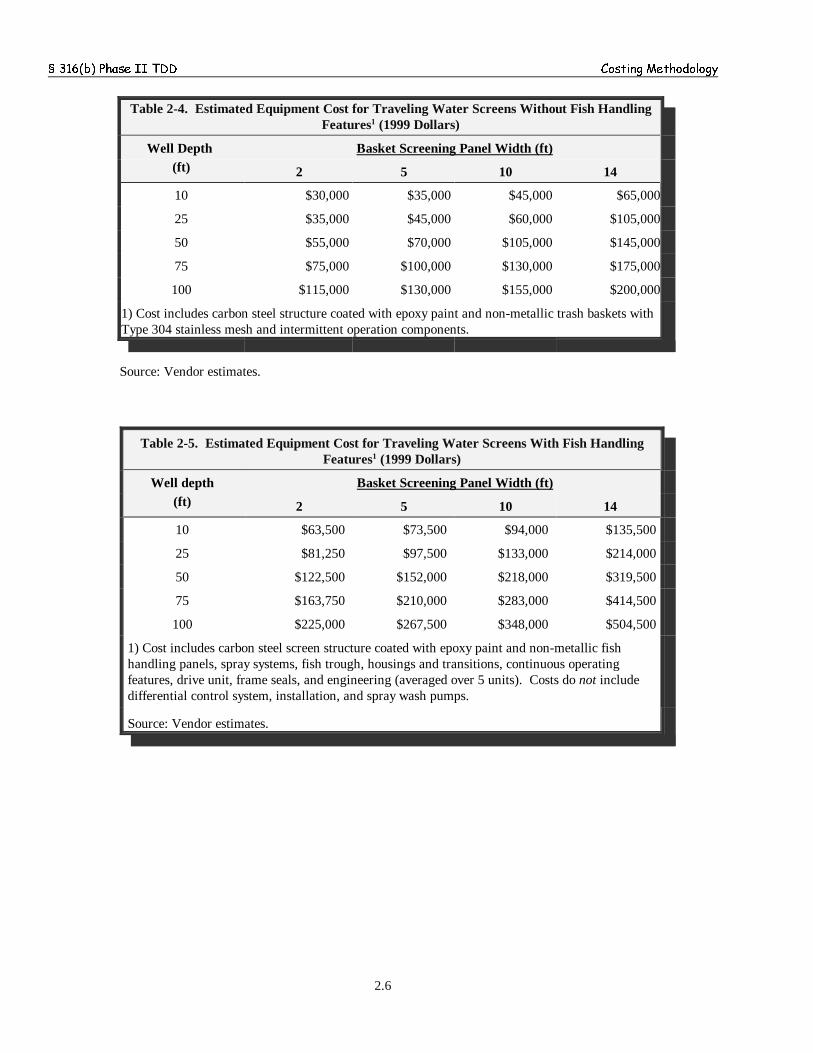
§ 316(b) Phase II TDD Costing Methodology
2.6
Table 2-4. Estimated Equipment Cost for Traveling Water Screens Without Fish HandlingFeatures1 (1999 Dollars)
Well Depth (ft)
Basket Screening Panel Width (ft)
2 5 10 14
10 $30,000 $35,000 $45,000 $65,000
25 $35,000 $45,000 $60,000 $105,000
50 $55,000 $70,000 $105,000 $145,000
75 $75,000 $100,000 $130,000 $175,000
100 $115,000 $130,000 $155,000 $200,000
1) Cost includes carbon steel structure coated with epoxy paint and non-metallic trash baskets withType 304 stainless mesh and intermittent operation components.
Source: Vendor estimates.
Table 2-5. Estimated Equipment Cost for Traveling Water Screens With Fish HandlingFeatures1 (1999 Dollars)
Well depth(ft)
Basket Screening Panel Width (ft)
2 5 10 14
10 $63,500 $73,500 $94,000 $135,500
25 $81,250 $97,500 $133,000 $214,000
50 $122,500 $152,000 $218,000 $319,500
75 $163,750 $210,000 $283,000 $414,500
100 $225,000 $267,500 $348,000 $504,500
1) Cost includes carbon steel screen structure coated with epoxy paint and non-metallic fishhandling panels, spray systems, fish trough, housings and transitions, continuous operatingfeatures, drive unit, frame seals, and engineering (averaged over 5 units). Costs do not includedifferential control system, installation, and spray wash pumps.
Source: Vendor estimates.
§ 316(b) Phase II TDD Costing Methodology
2.7
Installation Cost
Installation costs of traveling screens for New Facilities are based on the following assumptions of a typical averageinstallation requirement for a hypothetical scenario. Site preparation and earth work are calculated based on thefollowing assumptions:
C Clearing and grubbing: Clearing light to medium brush up to 4" diameter with a bulldozer.
C Earthwork: Excavation of heavy soils. Quantity is based on the assumption that earthwork increases withscreen width.
C Paving and surfacing: Using concrete 8" thick and assuming that the cost of pavement attributed to screeninstallation is 6x3 yards for the smallest screen and 25x6 yards for the largest screen.
C Structural concrete: The structural concrete work attributed to screen installation is four 12"x12" reinforcedconcrete columns with depths varying between 1.5 yards and 3 yards. There is more structural concrete workfor a water intake structure, however, for new source screens and retrofit screens, only a portion of the intakestructural cost can be justifiably attributed to the screen costs. For new screens, most of the concrete structurework is for developing the site to make it accessible for equipment and protect it from hydraulic elements,which are necessary for constructing the intake itself. For retrofits, some of the structural concrete will alreadyexist and some of it will not be needed since the intake is already in place and only the screen needs to beinstalled. All unit costs used in calculating on-shore site preparation were obtained from Heavy ConstructionCost Data 1998 (R. S. Means, 1997b).
Table 2-6 presents site preparation installation costs that apply to traveling screens both with and without fish handlingfeatures. The total onshore construction costs are for a screen to be installed in a 10-foot well depth. Screens to beinstalled in deeper water are assumed to require additional site preparation work. Hence for costing purposes it isassumed that site preparation costs increase at a rate of an additional 25 percent per depth factor (calculated as the ratioof the well depth to the base well depth of 10 feet) for well depths greater than 10 feet. Table 2-7 presents the estimatedcosts of site preparation for four sizes of screen widths and various well depths.
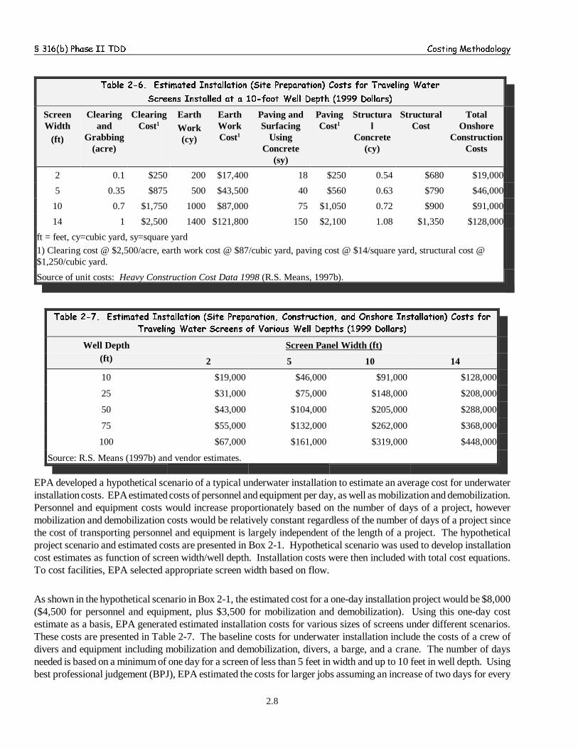
§ 316(b) Phase II TDD Costing Methodology
2.8
Table 2-6. Estimated Installation (Site Preparation) Costs for Traveling Water
Screens Installed at a 10-foot Well Depth (1999 Dollars)
ScreenWidth
(ft)
Clearingand
Grabbing(acre)
ClearingCost1
EarthWork(cy)
EarthWorkCost1
Paving andSurfacing
UsingConcrete
(sy)
PavingCost1
Structural
Concrete(cy)
StructuralCost
TotalOnshore
ConstructionCosts
2 0.1 $250 200 $17,400 18 $250 0.54 $680 $19,000
5 0.35 $875 500 $43,500 40 $560 0.63 $790 $46,000
10 0.7 $1,750 1000 $87,000 75 $1,050 0.72 $900 $91,000
14 1 $2,500 1400 $121,800 150 $2,100 1.08 $1,350 $128,000
ft = feet, cy=cubic yard, sy=square yard
1) Clearing cost @ $2,500/acre, earth work cost @ $87/cubic yard, paving cost @ $14/square yard, structural cost @$1,250/cubic yard.
Source of unit costs: Heavy Construction Cost Data 1998 (R.S. Means, 1997b).
Table 2-7. Estimated Installation (Site Preparation, Construction, and Onshore Installation) Costs for
Traveling Water Screens of Various Well Depths (1999 Dollars)
Well Depth(ft)
Screen Panel Width (ft)
2 5 10 14
10 $19,000 $46,000 $91,000 $128,000
25 $31,000 $75,000 $148,000 $208,000
50 $43,000 $104,000 $205,000 $288,000
75 $55,000 $132,000 $262,000 $368,000
100 $67,000 $161,000 $319,000 $448,000
Source: R.S. Means (1997b) and vendor estimates.
EPA developed a hypothetical scenario of a typical underwater installation to estimate an average cost for underwaterinstallation costs. EPA estimated costs of personnel and equipment per day, as well as mobilization and demobilization.Personnel and equipment costs would increase proportionately based on the number of days of a project, howevermobilization and demobilization costs would be relatively constant regardless of the number of days of a project sincethe cost of transporting personnel and equipment is largely independent of the length of a project. The hypotheticalproject scenario and estimated costs are presented in Box 2-1. Hypothetical scenario was used to develop installationcost estimates as function of screen width/well depth. Installation costs were then included with total cost equations.To cost facilities, EPA selected appropriate screen width based on flow.
As shown in the hypothetical scenario in Box 2-1, the estimated cost for a one-day installation project would be $8,000($4,500 for personnel and equipment, plus $3,500 for mobilization and demobilization). Using this one-day costestimate as a basis, EPA generated estimated installation costs for various sizes of screens under different scenarios.These costs are presented in Table 2-7. The baseline costs for underwater installation include the costs of a crew ofdivers and equipment including mobilization and demobilization, divers, a barge, and a crane. The number of daysneeded is based on a minimum of one day for a screen of less than 5 feet in width and up to 10 feet in well depth. Usingbest professional judgement (BPJ), EPA estimated the costs for larger jobs assuming an increase of two days for every
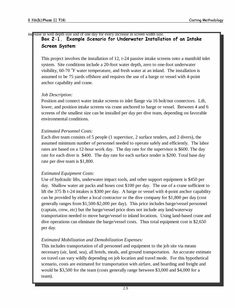
§ 316(b) Phase II TDD Costing Methodology
2.9
Box 2-1. Example Scenario for Underwater Installation of an Intake
Screen System
This project involves the installation of 12, t-24 passive intake screens onto a manifold inletsystem. Site conditions include a 20-foot water depth, zero to one-foot underwatervisibility, 60-70 NF water temperature, and fresh water at an inland. The installation isassumed to be 75 yards offshore and requires the use of a barge or vessel with 4-pointanchor capability and crane.
Job Description:Position and connect water intake screens to inlet flange via 16 bolt/nut connectors. Lift,lower, and position intake screens via crane anchored to barge or vessel. Between 4 and 6screens of the smallest size can be installed per day per dive team, depending on favorableenvironmental conditions.
Estimated Personnel Costs:Each dive team consists of 5 people (1 supervisor, 2 surface tenders, and 2 divers), theassumed minimum number of personnel needed to operate safely and efficiently. The laborrates are based on a 12-hour work day. The day rate for the supervisor is $600. The dayrate for each diver is $400. The day rate for each surface tender is $200. Total base dayrate per dive team is $1,800.
Estimated Equipment Costs:Use of hydraulic lifts, underwater impact tools, and other support equipment is $450 perday. Shallow water air packs and hoses cost $100 per day. The use of a crane sufficient tolift the 375 lb t-24 intakes is $300 per day. A barge or vessel with 4-point anchor capabilitycan be provided by either a local contractor or the dive company for $1,800 per day (costgenerally ranges from $1,500-$2,000 per day). This price includes barge/vessel personnel(captain, crew, etc) but the barge/vessel price does not include any land/waterwaytransportation needed to move barge/vessel to inland locations. Using land-based crane anddive operations can eliminate the barge/vessel costs. Thus total equipment cost is $2,650per day.
Estimated Mobilization and Demobilization Expenses:This includes transportation of all personnel and equipment to the job site via meansnecessary (air, land, sea), all hotels, meals, and ground transportation. An accurate estimateon travel can vary wildly depending on job location and travel mode. For this hypotheticalscenario, costs are estimated for transportation with airfare, and boarding and freight andwould be $3,500 for the team (costs generally range between $3,000 and $4,000 for ateam).
increase in well depth size and of one day for every increase in screen width size.
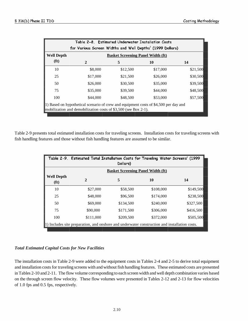
§ 316(b) Phase II TDD Costing Methodology
2.10
Table 2-8. Estimated Underwater Installation Costs
for Various Screen Widths and Well Depths1 (1999 Dollars)
Well Depth(ft)
Basket Screening Panel Width (ft)
2 5 10 14
10 $8,000 $12,500 $17,000 $21,500
25 $17,000 $21,500 $26,000 $30,500
50 $26,000 $30,500 $35,000 $39,500
75 $35,000 $39,500 $44,000 $48,500
100 $44,000 $48,500 $53,000 $57,500
1) Based on hypothetical scenario of crew and equipment costs of $4,500 per day andmobilization and demobilization costs of $3,500 (see Box 2-1).
Table 2-9 presents total estimated installation costs for traveling screens. Installation costs for traveling screens withfish handling features and those without fish handling features are assumed to be similar.
Table 2-9. Estimated Total Installation Costs for Traveling Water Screens1 (1999
Dollars)
Well Depth(ft)
Basket Screening Panel Width (ft)
2 5 10 14
10 $27,000 $58,500 $108,000 $149,500
25 $48,000 $96,500 $174,000 $238,500
50 $69,000 $134,500 $240,000 $327,500
75 $90,000 $171,500 $306,000 $416,500
100 $111,000 $209,500 $372,000 $505,500
1) Includes site preparation, and onshore and underwater construction and installation costs.
Total Estimated Capital Costs for New Facilities
The installation costs in Table 2-9 were added to the equipment costs in Tables 2-4 and 2-5 to derive total equipmentand installation costs for traveling screens with and without fish handling features. These estimated costs are presentedin Tables 2-10 and 2-11. The flow volume corresponding to each screen width and well depth combination varies basedon the through screen flow velocity. These flow volumes were presented in Tables 2-12 and 2-13 for flow velocitiesof 1.0 fps and 0.5 fps, respectively.
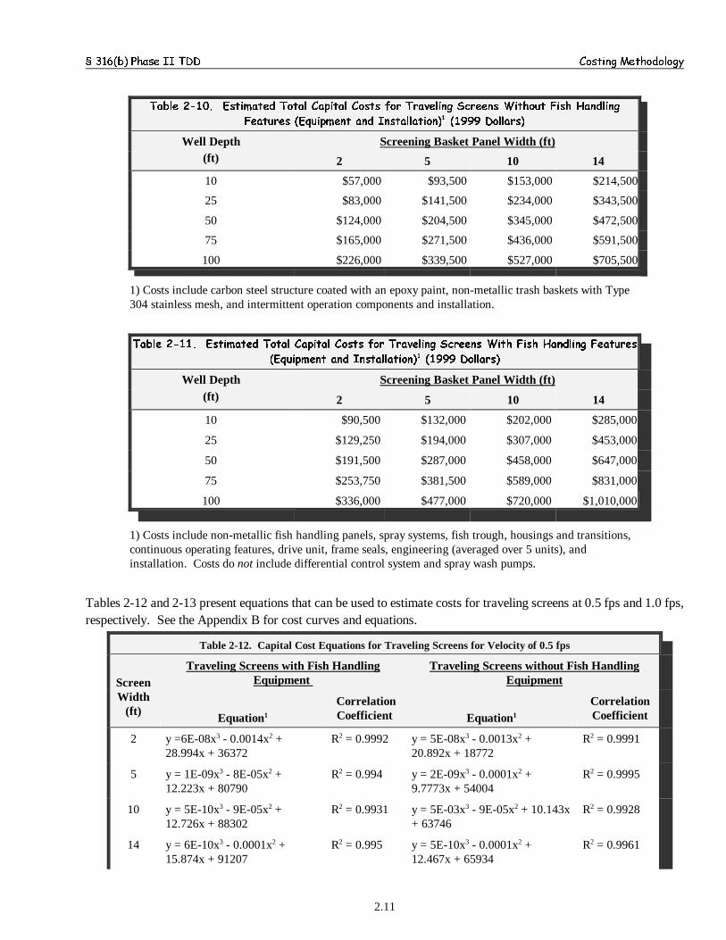
§ 316(b) Phase II TDD Costing Methodology
2.11
Table 2-10. Estimated Total Capital Costs for Traveling Screens Without Fish Handling
Features (Equipment and Installation)1 (1999 Dollars)
Well Depth(ft)
Screening Basket Panel Width (ft)
2 5 10 14
10 $57,000 $93,500 $153,000 $214,500
25 $83,000 $141,500 $234,000 $343,500
50 $124,000 $204,500 $345,000 $472,500
75 $165,000 $271,500 $436,000 $591,500
100 $226,000 $339,500 $527,000 $705,500
1) Costs include carbon steel structure coated with an epoxy paint, non-metallic trash baskets with Type304 stainless mesh, and intermittent operation components and installation.
Table 2-11. Estimated Total Capital Costs for Traveling Screens With Fish Handling Features
(Equipment and Installation)1 (1999 Dollars)
Well Depth(ft)
Screening Basket Panel Width (ft)
2 5 10 14
10 $90,500 $132,000 $202,000 $285,000
25 $129,250 $194,000 $307,000 $453,000
50 $191,500 $287,000 $458,000 $647,000
75 $253,750 $381,500 $589,000 $831,000
100 $336,000 $477,000 $720,000 $1,010,000
1) Costs include non-metallic fish handling panels, spray systems, fish trough, housings and transitions,continuous operating features, drive unit, frame seals, engineering (averaged over 5 units), andinstallation. Costs do not include differential control system and spray wash pumps.
Tables 2-12 and 2-13 present equations that can be used to estimate costs for traveling screens at 0.5 fps and 1.0 fps,respectively. See the Appendix B for cost curves and equations.
Table 2-12. Capital Cost Equations for Traveling Screens for Velocity of 0.5 fps
ScreenWidth
(ft)
Traveling Screens with Fish HandlingEquipment
Traveling Screens without Fish HandlingEquipment
Equation1
CorrelationCoefficient Equation1
CorrelationCoefficient
2 y =6E-08x3 - 0.0014x2 +28.994x + 36372
R2 = 0.9992 y = 5E-08x3 - 0.0013x2 +20.892x + 18772
R2 = 0.9991
5 y = 1E-09x3 - 8E-05x2 +12.223x + 80790
R2 = 0.994 y = 2E-09x3 - 0.0001x2 +9.7773x + 54004
R2 = 0.9995
10 y = 5E-10x3 - 9E-05x2 +12.726x + 88302
R2 = 0.9931 y = 5E-03x3 - 9E-05x2 + 10.143x+ 63746
R2 = 0.9928
14 y = 6E-10x3 - 0.0001x2 +15.874x + 91207
R2 = 0.995 y = 5E-10x3 - 0.0001x2 +12.467x + 65934
R2 = 0.9961
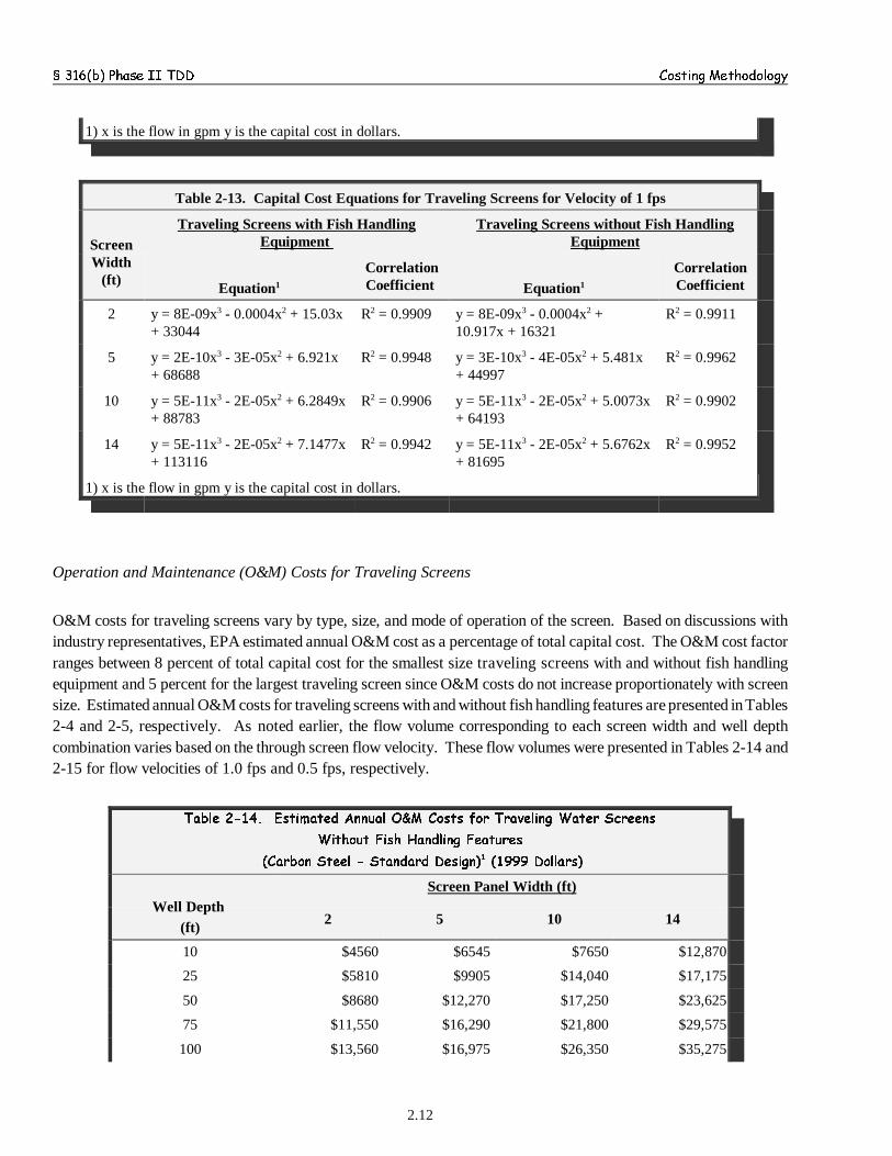
§ 316(b) Phase II TDD Costing Methodology
2.12
1) x is the flow in gpm y is the capital cost in dollars.
Table 2-13. Capital Cost Equations for Traveling Screens for Velocity of 1 fps
ScreenWidth
(ft)
Traveling Screens with Fish HandlingEquipment
Traveling Screens without Fish HandlingEquipment
Equation1
CorrelationCoefficient Equation1
CorrelationCoefficient
2 y = 8E-09x3 - 0.0004x2 + 15.03x+ 33044
R2 = 0.9909 y = 8E-09x3 - 0.0004x2 +10.917x + 16321
R2 = 0.9911
5 y = 2E-10x3 - 3E-05x2 + 6.921x+ 68688
R2 = 0.9948 y = 3E-10x3 - 4E-05x2 + 5.481x+ 44997
R2 = 0.9962
10 y = 5E-11x3 - 2E-05x2 + 6.2849x+ 88783
R2 = 0.9906 y = 5E-11x3 - 2E-05x2 + 5.0073x+ 64193
R2 = 0.9902
14 y = 5E-11x3 - 2E-05x2 + 7.1477x+ 113116
R2 = 0.9942 y = 5E-11x3 - 2E-05x2 + 5.6762x+ 81695
R2 = 0.9952
1) x is the flow in gpm y is the capital cost in dollars.
Operation and Maintenance (O&M) Costs for Traveling Screens
O&M costs for traveling screens vary by type, size, and mode of operation of the screen. Based on discussions withindustry representatives, EPA estimated annual O&M cost as a percentage of total capital cost. The O&M cost factorranges between 8 percent of total capital cost for the smallest size traveling screens with and without fish handlingequipment and 5 percent for the largest traveling screen since O&M costs do not increase proportionately with screensize. Estimated annual O&M costs for traveling screens with and without fish handling features are presented in Tables2-4 and 2-5, respectively. As noted earlier, the flow volume corresponding to each screen width and well depthcombination varies based on the through screen flow velocity. These flow volumes were presented in Tables 2-14 and2-15 for flow velocities of 1.0 fps and 0.5 fps, respectively.
Table 2-14. Estimated Annual O&M Costs for Traveling Water Screens
Without Fish Handling Features
(Carbon Steel - Standard Design)1 (1999 Dollars)
Well Depth (ft)
Screen Panel Width (ft)
2 5 10 14
10 $4560 $6545 $7650 $12,870
25 $5810 $9905 $14,040 $17,175
50 $8680 $12,270 $17,250 $23,625
75 $11,550 $16,290 $21,800 $29,575
100 $13,560 $16,975 $26,350 $35,275

§ 316(b) Phase II TDD Costing Methodology
2.13
1) Annual O&M costs range between 8 percent of total capital cost for the smallest size travelingscreens with and without fish handling equipment and 5 percent for the largest traveling screen.
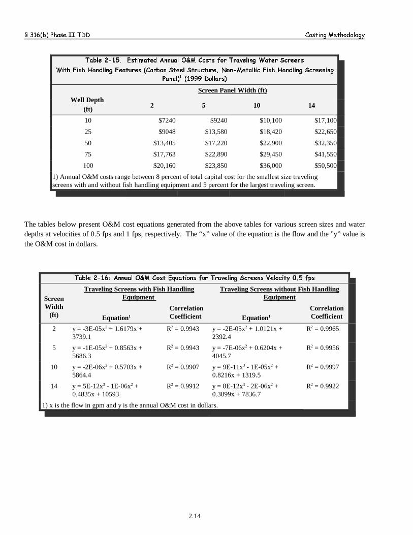
§ 316(b) Phase II TDD Costing Methodology
2.14
Table 2-15. Estimated Annual O&M Costs for Traveling Water Screens
With Fish Handling Features (Carbon Steel Structure, Non-Metallic Fish Handling Screening
Panel)1 (1999 Dollars)
Well Depth (ft)
Screen Panel Width (ft)
2 5 10 14
10 $7240 $9240 $10,100 $17,100
25 $9048 $13,580 $18,420 $22,650
50 $13,405 $17,220 $22,900 $32,350
75 $17,763 $22,890 $29,450 $41,550
100 $20,160 $23,850 $36,000 $50,500
1) Annual O&M costs range between 8 percent of total capital cost for the smallest size travelingscreens with and without fish handling equipment and 5 percent for the largest traveling screen.
The tables below present O&M cost equations generated from the above tables for various screen sizes and waterdepths at velocities of 0.5 fps and 1 fps, respectively. The “x” value of the equation is the flow and the ”y” value isthe O&M cost in dollars.
Table 2-16: Annual O&M Cost Equations for Traveling Screens Velocity 0.5 fps
ScreenWidth
(ft)
Traveling Screens with Fish HandlingEquipment
Traveling Screens without Fish HandlingEquipment
Equation1
CorrelationCoefficient Equation1
CorrelationCoefficient
2 y = -3E-05x2 + 1.6179x +3739.1
R2 = 0.9943 y = -2E-05x2 + 1.0121x +2392.4
R2 = 0.9965
5 y = -1E-05x2 + 0.8563x +5686.3
R2 = 0.9943 y = -7E-06x2 + 0.6204x +4045.7
R2 = 0.9956
10 y = -2E-06x2 + 0.5703x +5864.4
R2 = 0.9907 y = 9E-11x3 - 1E-05x2 +0.8216x + 1319.5
R2 = 0.9997
14 y = 5E-12x3 - 1E-06x2 +0.4835x + 10593
R2 = 0.9912 y = 8E-12x3 - 2E-06x2 +0.3899x + 7836.7
R2 = 0.9922
1) x is the flow in gpm and y is the annual O&M cost in dollars.
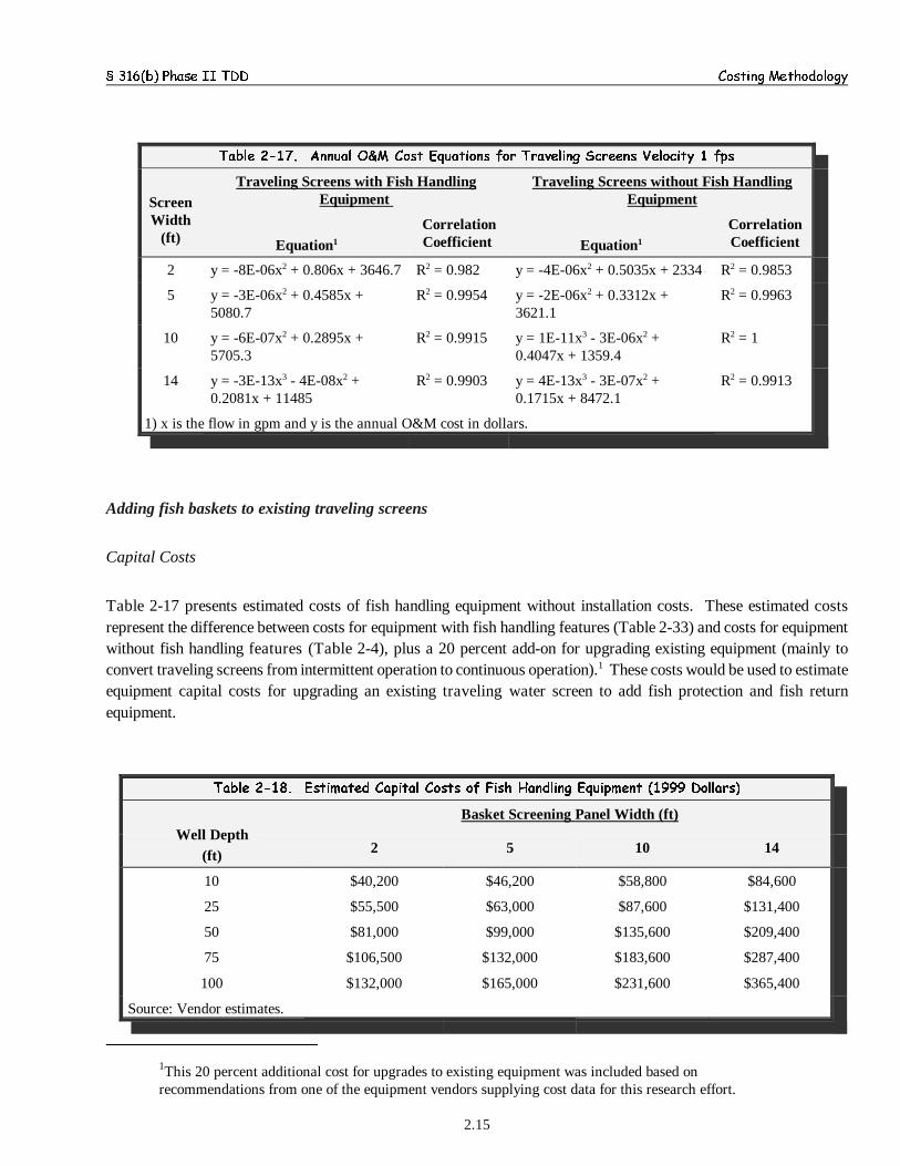
§ 316(b) Phase II TDD Costing Methodology
1This 20 percent additional cost for upgrades to existing equipment was included based onrecommendations from one of the equipment vendors supplying cost data for this research effort.
2.15
Table 2-17. Annual O&M Cost Equations for Traveling Screens Velocity 1 fps
ScreenWidth
(ft)
Traveling Screens with Fish HandlingEquipment
Traveling Screens without Fish HandlingEquipment
Equation1
CorrelationCoefficient Equation1
CorrelationCoefficient
2 y = -8E-06x2 + 0.806x + 3646.7 R2 = 0.982 y = -4E-06x2 + 0.5035x + 2334 R2 = 0.9853
5 y = -3E-06x2 + 0.4585x +5080.7
R2 = 0.9954 y = -2E-06x2 + 0.3312x +3621.1
R2 = 0.9963
10 y = -6E-07x2 + 0.2895x +5705.3
R2 = 0.9915 y = 1E-11x3 - 3E-06x2 +0.4047x + 1359.4
R2 = 1
14 y = -3E-13x3 - 4E-08x2 +0.2081x + 11485
R2 = 0.9903 y = 4E-13x3 - 3E-07x2 +0.1715x + 8472.1
R2 = 0.9913
1) x is the flow in gpm and y is the annual O&M cost in dollars.
Adding fish baskets to existing traveling screens
Capital Costs
Table 2-17 presents estimated costs of fish handling equipment without installation costs. These estimated costsrepresent the difference between costs for equipment with fish handling features (Table 2-33) and costs for equipmentwithout fish handling features (Table 2-4), plus a 20 percent add-on for upgrading existing equipment (mainly toconvert traveling screens from intermittent operation to continuous operation).1 These costs would be used to estimateequipment capital costs for upgrading an existing traveling water screen to add fish protection and fish returnequipment.
Table 2-18. Estimated Capital Costs of Fish Handling Equipment (1999 Dollars)
Well Depth(ft)
Basket Screening Panel Width (ft)
2 5 10 14
10 $40,200 $46,200 $58,800 $84,600
25 $55,500 $63,000 $87,600 $131,400
50 $81,000 $99,000 $135,600 $209,400
75 $106,500 $132,000 $183,600 $287,400
100 $132,000 $165,000 $231,600 $365,400
Source: Vendor estimates.
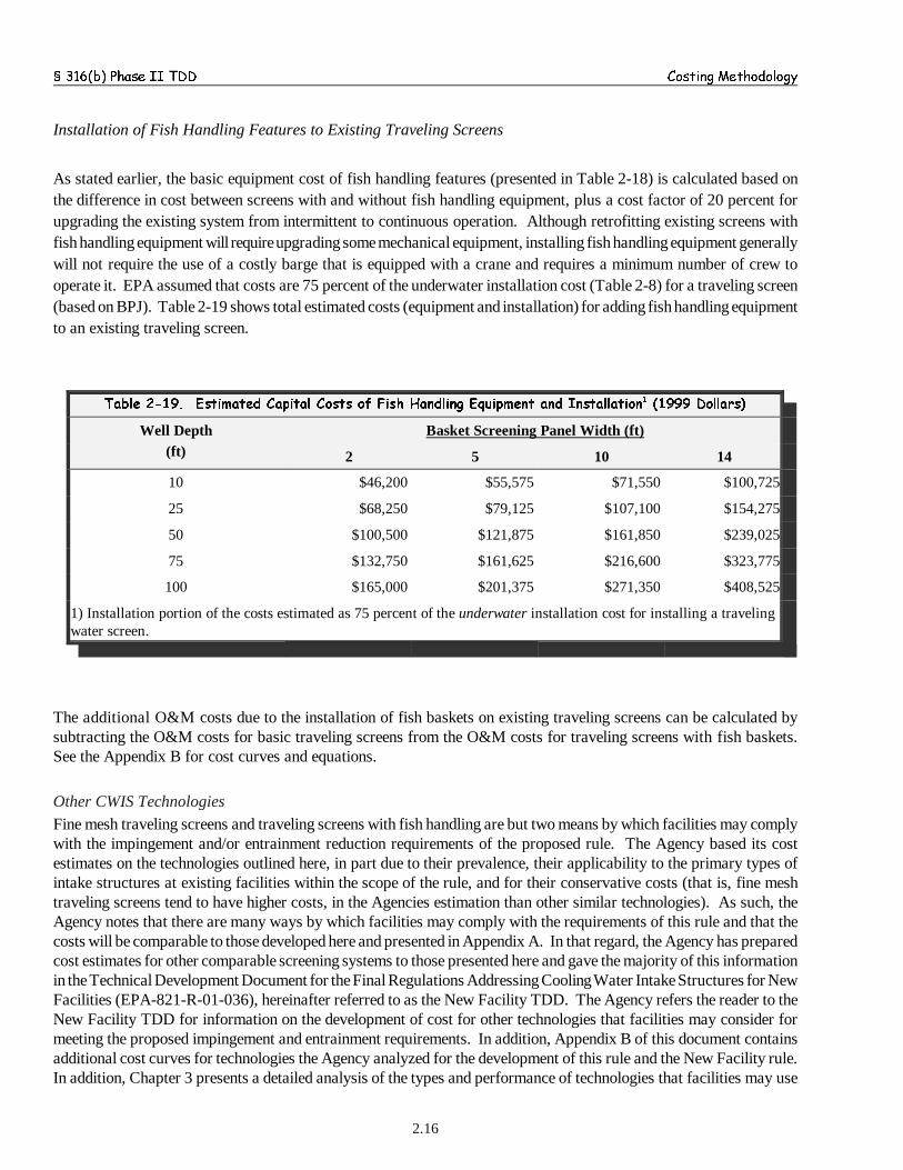
§ 316(b) Phase II TDD Costing Methodology
2.16
Installation of Fish Handling Features to Existing Traveling Screens
As stated earlier, the basic equipment cost of fish handling features (presented in Table 2-18) is calculated based onthe difference in cost between screens with and without fish handling equipment, plus a cost factor of 20 percent forupgrading the existing system from intermittent to continuous operation. Although retrofitting existing screens withfish handling equipment will require upgrading some mechanical equipment, installing fish handling equipment generallywill not require the use of a costly barge that is equipped with a crane and requires a minimum number of crew tooperate it. EPA assumed that costs are 75 percent of the underwater installation cost (Table 2-8) for a traveling screen(based on BPJ). Table 2-19 shows total estimated costs (equipment and installation) for adding fish handling equipmentto an existing traveling screen.
Table 2-19. Estimated Capital Costs of Fish Handling Equipment and Installation1 (1999 Dollars)
Well Depth(ft)
Basket Screening Panel Width (ft)
2 5 10 14
10 $46,200 $55,575 $71,550 $100,725
25 $68,250 $79,125 $107,100 $154,275
50 $100,500 $121,875 $161,850 $239,025
75 $132,750 $161,625 $216,600 $323,775
100 $165,000 $201,375 $271,350 $408,525
1) Installation portion of the costs estimated as 75 percent of the underwater installation cost for installing a travelingwater screen.
The additional O&M costs due to the installation of fish baskets on existing traveling screens can be calculated bysubtracting the O&M costs for basic traveling screens from the O&M costs for traveling screens with fish baskets.See the Appendix B for cost curves and equations.
Other CWIS Technologies
Fine mesh traveling screens and traveling screens with fish handling are but two means by which facilities may complywith the impingement and/or entrainment reduction requirements of the proposed rule. The Agency based its costestimates on the technologies outlined here, in part due to their prevalence, their applicability to the primary types ofintake structures at existing facilities within the scope of the rule, and for their conservative costs (that is, fine meshtraveling screens tend to have higher costs, in the Agencies estimation than other similar technologies). As such, theAgency notes that there are many ways by which facilities may comply with the requirements of this rule and that thecosts will be comparable to those developed here and presented in Appendix A. In that regard, the Agency has preparedcost estimates for other comparable screening systems to those presented here and gave the majority of this informationin the Technical Development Document for the Final Regulations Addressing Cooling Water Intake Structures for NewFacilities (EPA-821-R-01-036), hereinafter referred to as the New Facility TDD. The Agency refers the reader to theNew Facility TDD for information on the development of cost for other technologies that facilities may consider formeeting the proposed impingement and entrainment requirements. In addition, Appendix B of this document containsadditional cost curves for technologies the Agency analyzed for the development of this rule and the New Facility rule.In addition, Chapter 3 presents a detailed analysis of the types and performance of technologies that facilities may use

§ 316(b) Phase II TDD Costing Methodology
2.17
to comply with the proposed existing facility rule.
2.2 OUTLINE OF COOLING SYSTEM CONVERSION COSTING METHODOLOGY
Under certain regulatory options considered (those described in Chapter 4.3), existing facilities are projected to installrecirculating wet cooling systems. The Agency developed a methodology for estimating the costs of converting model-facility cooling systems from once-through to recirculating operation in the effort of reproducing the costs andengineering characteristics of the example cooling system conversion cases presented in Chapter 4. The methodologyfor estimating costs of these cooling system conversions is based on the principles observed in the empirical cases andin historical proposals for cooling system conversions (see Chapter 4 for more discussion). The commonalities and/orprinciples are as follows:
- recirculating systems can be connected to the existing condensers and operated successfully under a varietyof conditions (but not all);
- condenser flows generally do not change due to the conversions;
- significant portions of the condenser conduit systems can be used for the recirculating tower systems;
- existing cooling water pumps generally would be replaced with new circulating water pumps or boosterpumps would be installed to increase pumping energy of the circulating system;
- the existing intake structures can be used for supplying make-up water to the recirculating towers (thoughdemolition and replacement of the intake pumps may be necessary);
- pumping distances from tower systems to condensers can be significant, but existing piping runs can, insome cases, be utilized to reduce the amount of new circulating piping installed;
- tower structures can be constructed on-site before connection to the existing conduit system; and
- modification and branching of circulating piping is necessary for connecting the recirculating system tothe existing conduits and for providing make-up water to the towers.
Based on these principles, the Agency developed cost estimates for cooling system conversions utilizing those developedfor new, “greenfield” facilities and inflated these costs by a “retrofit” factor to account for activities outside the scopeof the “greenfield” cost estimates. See sections 2.1 and 2.2 for the cost estimates for “greenfield” cooling tower systemsand intake structures. See section 2.6 for a discussion of the “retrofit” factor.
Condenser Refurbishments for Cooling System Conversions
The Agency includes costs for condenser refurbishments at a subset of facilities expected to comply with flow reductionrequirements in the regulatory options considered. The Agency projects premature condenser refurbishments, in part,to alleviate potential condenser tube failures, such as that experienced at the Palisades plant. The Agency researchedthe materials of construction of surface condensers for the model plants under certain regulatory options and for theexample cases described in Chapter 4. The Agency also consulted with condenser manufacturing representatives foradvice on probable causes for condenser failures due to cooling system conversions, motivations for condenserreplacements or refurbishments, useful lives of condensers, and appropriate tube materials for recirculating coolingsystems for a variety of water types. Of the four example cases in Chapter 4, only the Palisades plant experiencedcondenser failure potentially related to the cooling system conversion. Plant personnel were not able to confirm thecondenser tube material at the time of the failure, nor were they able to positively confirm the cause of the failure asrelating to the recirculating system. Hence, the Agency could not isolate the specific cause of the Palisades failure and,therefore, relied on additional information to determine which plants would likely replace condensers in order to upgrade
§ 316(b) Phase II TDD Costing Methodology
2.18
the cooling system under certain regulatory options. The Agency learned from condenser vendors that plants wouldelect to upgrade condenser tube materials to increase the efficiency of the recirculating cooling system. In addition,based on the circumstantial evidence that the Palisades failure happened, at least in part, due to the chemical additionnecessary for the recirculating system and the fact that many of the plants projected to upgrade their cooling systemsunder certain regulatory options utilize brackish or saline cooling water, the Agency judged that the material of the tubeswould need to withstand corrosive effects of chemical addition and increased salt content of the cooling water (due toconcentration in a recirculating system). Hence, the Agency concluded that meeting a baseline standard of condensertube material would determine which model plants would most likely upgrade condenser tube materials. See section3.2.4 for further information on condenser refurbishments.
Condenser Flows for Cooling System Conversions
Based on the example cases of cooling system conversions in Chapter 4, the Agency determined that condenserflows would not change as a result of cooling system upgrades. The cooling water flow through these tube bundleswould be the same as for the once-through systems due to the fact that each of the example cases utilized the original,once-through designed, cooling water flow. In addition to the empirical example cases, the Agency researchedcondenser flow to MW ratios to determine if cooling system type influenced the flow rate to capacity ratio. Publishedcondenser flows and generating capacity data from the Nuclear Regulatory Commission (DCN 4-2521)) for all nuclearunits in the US demonstrates that recirculating cooling systems have lower condenser flow to MW ratios than once-through systems, regardless of age or other characteristics. After considering this information, EPA chose aconservative approach and used the design cooling water intake flow of the baseline once-through system intake toestimate the size of the recirculating cooling tower and associated conduit system for its model facilities. EPA notesthat design flows are significantly higher than operating flows in some cases. As such, the approach of the Agency isadditionally conservative, in that facilities considering cooling system conversions could optimize the design of thecirculating flow levels appropriate for the facilities operating flows if sufficient unused design intake capacity exists.
Reuse of Existing Intake Structures for Supplying Make-up Water to Cooling Towers
As demonstrated by the example cases in Chapter 4, conversions from once-through to recirculating coolingsystems do not require construction of new intake structures to provide make-up water to the cooling tower systems.Installation of a fully recirculating cooling system reduces intake flow by upwards of approximately 92 percent ascompared to a once-through system. In turn the intake structure designed for a once-through cooling system is oversizedfor moving flows reduced to this level. For the case of the Palisades plant, the original intake structure withdrew waterfrom a submerged offshore intake. The plant continued to utilize this intake structure (a velocity cap) and the associatedsubmerged piping system (3300 ft) after the conversion. A branch from the onshore portion of the original intakeconduit system provided make-up flow to the cooling tower via a separate pump system. The Agency includes capitalcosts for the conduit system required to bring make-up water to the cooling tower and basin. See Example 1 of thischapter for a discussion of the makeup and blowdown piping associated with the Agency’s cooling system conversionestimates. The Agency includes these costs to account for conversion cases in which significant distances may existbetween intake locations and cooling tower sites. The Agency notes, as described in Example 1, that these pipingcapital costs are further inflated by the “retrofit” factor to account for construction techniques and situations outsidethe scope of a typical “greenfield” cost estimate. In turn, the Agency views the inclusion of these cost estimates asconservative and appropriate for cooling system conversions.
Cooling Tower Construction and Conduit Connections
The actual process of adjoining the cooling tower system to the existing condenser conduit system is reported
§ 316(b) Phase II TDD Costing Methodology
2.19
to have not disrupted service significantly for two of the example cases presented in Chapter 4. However, for thePalisades plant, Consumers Energy report that the outage lasted approximately 10 months for connection and start-upof the cooling tower system (see Chapter 4). The Agency estimates for the flow-reduction regulatory options consideredthat the typical process of adjoining the recirculating system to the existing condenser unit and the refurbishment of theexisting condenser (when necessary) would last approximately two months. Because the Agency analyzed flexiblecompliance dates (extended over a five-year compliance period), the Agency estimated that plants under the flow-reduction regulatory options could plan the cooling system conversion to coincide with periodic scheduled outages, aswas the case for the example cases. For the case of nuclear units, these outages can coincide with periodic inspections(ISIs) and refueling. For the case of fossil-fuel and combined-cycle units, the conversion can be planned to coincidewith periodic maintenance. Even though ISIs for nuclear units last typically 2 to 4 months, which would extend equalto or beyond the time required to connect the converted system, the Agency estimates for all model plants one monthof interrupted service due to the cooling system conversion. For further information see Chapter 4 of this documentand the EBA.
Connections of circulating systems to existing once-through conduits, in the Agency’s view, would occurthrough either demolition and/or removal of the connecting piping and/or through branching (and plugging) of theexisting conduit system outside the condenser buildings. The Agency estimates that the primary activities fall withinthe scope of types of construction projects accounted for by the “retrofit” capital cost inflation factor (see Section 2.6below). Note that the Agency applies the “retrofit” factor to each capital cost outlay for the entire project. Therefore,the branching/connection of the cooling system conduit system could be accounted for in the inflation of a variety ofcost components.
2.2.1 Capital Costs of Wet Towers
As described in section 2.2, above, in order to develop cooling system conversion costs for existing facilities, the Agencymodified the capital cost estimates for wet cooling tower systems that it developed for new, “greenfield” facilities inthe 316b Phase I Rule for New Facilities by applying a “retrofit” factor. The description of the Agency’s cost estimatesfor cooling tower systems at new facilities is presented below:
For cooling towers, EPA developed cost estimates for use at a range of different total recirculating flow volumes. Thecost for flow reduction technologies depends on many factors, including site-specific conditions. The Agencydetermined that the factor that is most relevant is the total flow. Therefore, EPA selected total flow as the factor onwhich to base unit costs and thus use for basic cost comparisons.
The maximum cooling flow value used to develop the wet tower cost equations (both Capital and O&M) was 204,000gpm. If the model facility flow value exceeded this maximum by 10 percent (i.e., > 225,000 gpm), EPA costed multipleparallel wet tower units.
Recirculating the cooling water in a system vastly reduces the amount of cooling water needed. The method mostfrequently used to cool the water in a recirculating system is putting the cooling water through a cooling tower.Therefore, EPA chose to cost cooling towers as the technology used to switch a once-through cooling system to arecirculating system.
The factors that generally have the greatest impact on cost are the flow, approach (the difference between cold watertemperature and ambient wet bulb temperature), tower type, and environmental considerations. Physical site conditions

§ 316(b) Phase II TDD Costing Methodology
2 In developing cost estimates for hybrid-wet/dry cooling towers included in Charts 2-1 through 2-6 of theattachments to this chapter, the Agency computed the capital costs of the hybrid tower unit according to the factorsreferenced here. The Agency then applied an inflation factor to account for the auxiliary components of installationof a cooling tower system. However, this may overstate the costs of hybrid towers in comparison to wet (only)systems, for the fact that hybrid and wet (only) towers would have roughly identical installation costs (see AppendixC of this document for a discussion of the installation costs of hybrid towers and Chapter 6 for a discussion of therelative costs of plume abatement (that is, hybrid towers) versus wet (only) cooling towers).
3The approach is the difference between the cold water (tower effluent) temperature and the tower wetbulb temperature. This is also referred to as the design approach. For example, at design conditions with
2.20
(e.g., topographic conditions, soils and underground conditions, water quality) affect cost, but in most situations aresecondary to the primary cost factors. Relative capital and operation cost estimates for various types of cooling towersare estimated in literature (Mirsky et al. (1992), Mirsky and Bauthier (1997), and Mirsky (2000))2.
Other characteristics of cooling towers include:
C Air flow: Mechanical draft towers use fans to induce air flow, while natural draft (i.e., hyperbolic) towersinduce natural air flow by the chimney effect produced by the height and shape of the tower. For towers ofsimilar capacity, natural draft towers typically require significantly less land area and have lower power costs(i.e., fans to induce air flow are not needed) but have higher initial costs (particularly because they need to betaller) than mechanical draft towers. Both mechanical draft and natural draft towers can be designed for airto flow through the fill material using either a crossflow (air flows horizontally) or counterflow (air flowsvertically upward) design, while the water flows vertically downward. Counterflow towers tend to be moreefficient at achieving heat reduction but are generally more expensive to build and operate because clearanceneeded at the bottom of the tower means the tower needs to be taller.
C Mode of operation: Cooling towers can be either recirculating (water is returned to the condenser for reuse)or non-recirculating (tower effluent is discharged to a receiving waterbody and not reused). Facilities usingnon-recirculating types (i.e., “helper” towers) draw large flows for cooling and therefore do not provide fishprotection for §316(b) purposes, so the information in this chapter is not intended to address non-recirculatingtowers.
C Construction materials: Towers can be made from concrete, steel, wood, and/or fiberglass.
Capital Cost of Cooling Towers (New Facility Cost Development)
The volume of water needed for cooling depends on the following critical parameters: water temperature, make ofequipment to be used (e.g, G.E turbine vs. ABB turbine, turbine with heat recovery system and turbine without heatrecovery system), discharge permit limits, water quality (particularly for wet cooling towers), and type of wet coolingtower (i.e., whether it is a natural draft or a mechanical draft).
Two cooling tower industry managers with extensive experience in selling and installing cooling towers to power plantsand other industries provided information on how they estimate budget capital costs associated with a wet cooling tower.The rule of thumb they use is $30/gpm for an approach of 10 degrees and $50/gpm for an approach of 5 degrees.3 This
§ 316(b) Phase II TDD Costing Methodology
a delta or design approach of 5 degrees, the tower effluent and blowdown would be 5 degrees warmer thanthe wet bulb temperature. A smaller delta (or lower tower effluent temperature) requires a larger coolingtower and thus is more expensive.
4 With a 33 percent efficiency, one-third of the heat is converted to electric energy and two-thirds goes towaste heat in the cooling water.
2.21
cost is for a “small” tower (flow less than 10,000 gpm) and equipment associated with the “basic” tower, and does notinclude installation. Important auxiliary costs are included in the installation factor estimate listed below. Above10,000 gpm, to account for economy of scale, the unit cost was lowered by $5/gpm over the flow range up to 204,000gpm. For flows greater than 204,000 gpm, a facility may need to use multiple towers or a custom design. Combiningthis with the variability in cost among various cooling tower types, costs for various tower types and features werecalculated for the flows used.
To estimate costs specifically for installing and operating a particular cooling tower, important factors include:
C Condenser heat load and wet bulb temperature (or approach to wet bulb temperature): Largely determinethe size needed. Size is also affected by climate conditions.
C Plant fuel type and age/efficiency: Condenser discharge heat load per Megawatt varies greatly by plant type(nuclear thermal efficiency is about 33 percent to 35 percent, while newer oil-fired plants can have nearly 40percent thermal efficiency, and newer coal-fired plants can have nearly 38 percent thermal efficiency).4 Olderplants typically have lower thermal efficiency than new plants.
C Topography: May affect tower height and/or shape, and may increase construction costs due to subsurfaceconditions. For example, sites requiring significant blasting, use of piles, or a remote tower location willtypically have greater installation/construction cost.
C Material used for tower construction: Wood towers tend to be the least expensive, followed by fiberglassreinforced plastic, steel, and concrete. However, some industry sources claim that Redwood capital costs mightbe much higher compared to other wood cooling towers, particularly in the Northwest U.S., because Redwoodtrees are a protected species. Factors that affect the material used include chemical and mineral compositionof the cooling water, cost, aesthetics, and local/regional availability of materials.
Capital costs for the recirculating wet tower include costs for all installation components, such as site preparation andclearing, support foundation, electrical wiring and controls, basin and sump, cicrulating piping, blowdown watertreatment system, and recirculating pump and housing costs. Wet tower costs are based on cost data for redwoodtowers with splash fill and an approach of 10 oF taken from Chart 2-3 in the attachments to this chapter. This towerequation does not include make-up and blowdown piping, intake pumps, intake structure and screening technologies.
In order to account for the important auxiliary costs of installing the cooling tower system, the Agency obtainedestimates from industry representatives for installation costs as an inflation percentage of the installed cooling towerunit costs. The factor that EPA obtained is 80 percent, which experienced industry representatives described as theaverage installation inflation factor. The Agency used this factor to inflate the rule of thumb described above for 10

§ 316(b) Phase II TDD Costing Methodology
2.22
degree F approach towers (from approximately $30 / gpm to $54 / gpm for the total project cost of a small douglas firtower and from $25 / gpm to $ 45 / gpm for large fir towers). The Agency chose the median design approach of 10degrees F based on empirical data from recently installed cooling towers at a variety of geographic locations and plantsizes (See Attachment C to Chapter 5). Applying the factors provided in literature for converting from douglas firmaterial to other types of cooling towers, the Agency derived capital cost equations for basic cooling towers of douglasfir, redwood, concrete, steel, and fiberglass reinforced plastic. For example, using the Agency’s methodology for newfacilities, the installed cost of a basic 205,000 gpm fiberglass tower would be expressed as follows: $25 * 1.8 * 110/ 100 * 205,000 = $10,147,500 (in 1999 $). To accommodate the relatively standard application of splash fill theAgency additionally multiplied by the factor for splash fill from the literature tower factors. For example, using thenew facility methodology for the installation of a 205,000 gpm redwood tower with splash fill would be expressed asfollows: $25 * 1.8 * 120 / 100 * 112 / 100 * 205,000 = $12,398,400 (in 1999 $). The Agency developed a series ofthese calculations for each type of tower using the literature factors and fitted curves to the results. These curve fitsare presented in Appendix B of this document as Figures 2-1 through 2-6. The Agency determined that the median costmaterial was redwood, which is just slightly more expensive than fiberglass reinforced plastic. The Agency learnedfrom cooling tower vendors that fiberglass has become relatively standard for new facility installations, and thereforechose to use the median costs of the redwood because they slightly exceeded those of fiberglass. As such, the Agencyprimarily developed installed cooling tower costs for the new facility rule using the equation for redwood towers withsplash fill. The equation for an installed redwood mechanical-draft cooling tower unit with 10 degree F designapproach and splash fill is as follows:
y = -5E-5 x^2 + 70.721 x + 25393 , (in 1999 $)
where x = flow in gallons per minute, valid up to 225,000 gpm.
For existing facility estimates of cooling tower conversions at non-nuclear facilities, this equation is the startingpoint for assessing the conversion project costs. In addition to the retrofit factor described in Section 2.6 below, theAgency also added additional makeup and discharge piping capital costs according to the methodology presented inExample 2, which demonstrates how the Agency estimated cooling tower conversion costs for certain regulatoryoptions considered for this proposal.
Similarly, the Agency developed the following equation for the installation capital costs of mechanical-draftconcrete cooling tower systems with splash fill:
y = -6E-5 x^2 + 87.845 x + 31674 , (in 1999 $)
where x = flow in gallons per minute, valid up to 225,000 gpm.
This equation was used as the starting point for assessing cooling tower conversion project capital costs for nuclearfacilities for certain regulatory options of this proposed rule. See Example 2 for a demonstration of theincorporation of regional cost factors, the retrofit factor, and makeup and discharge piping costs with the abovecapital cost equation.
EPA obtained data for 20 cooling tower construction projects: nine Douglas fir towers, eight fiberglass towers, oneredwood tower, and two towers for which the construction material was unknown (for purposes of comparison,EPA compared these last two towers to predicted costs for redwood towers). In some cases, the project costs did
§ 316(b) Phase II TDD Costing Methodology
2.23
not include certain components such as pumps or basins. Where this was the case, EPA adjusted the project costsas follows:
• where project costs did not include pumps, EPA added $10/gpm to the project costs to account for pumps.
• where project costs did not include pumps and basins, EPA doubled the project costs to account for pumpsand basins.
Chart 2-7 in the attachments to this chapter compares actual, total capital costs for wet cooling tower projectsagainst predicted costs from EPA’s cooling tower capital cost curves, with 25 percent error bars around the costcurve predicted values. This chart shows that, in almost all cases, EPA’s cost curves provide conservative costestimates (erring on the high side) and are within 25 percent or less of actual project costs. In those few caseswhere the cost curve predictions are not within 25 percent of the actual costs, the difference can generally beattributed to the fact that the constructed cooling towers were designed for temperature approaches different thanthe 10 °F used for EPA’s cost curves.
For the existing facility regulatory options based on flow reduction, the Agency first compared the validity of theredwood cost curve against empirical turn key costs from cooling tower projects at existing facilities. The Agencyobtained four sets of total installed cooling tower costs for helper towers and expansions at existing facilities. TheAgency attempted to discern if construction costs at existing facilities were inherently different from its empiricallyverified cost equations for new facilities. The results of this analysis showed that the median $ per gpm predictionsof the redwood equation were nearly identical to those of the four existing facility projects (DCN 4522). However,the Agency determined that additional inflation of the new facility costs was necessary to compensate for theprobable additional costs that would be associated with cooling system conversions. In turn, the Agency estimateda retrofit factor of 20 percent additional installed capital cost would be necessary for an average retrofit project.
As described in Chapter 4, the Agency obtained two empirical, total project costs for cooling tower conversionprojects. The Agency calculated estimated project costs based on the methodology presented in Example 2 belowand determined that for the case of the Palisades conversion that the Agency’s methodology was very accurate. Forthe case of Pittsburg Unit 7, the Agency methodology for assessing conversion costs at non-nuclear plants mayhave understated total project capital costs (as reported by Pittsburg) by approximately 18 percent. In part, theAgency estimates that exclusion of makeup water pumps may have contributed to the difference (see Example 2). For more information on the on the cooling system example cases see Chapter 4 .
2.2.2 Operation and Maintenance Costs of Wet Towers
The Agency estimates that operation and maintenance costs of wet cooling tower systems for conversion projectswould be the same as those developed for new, “greenfield” facilities during the 316b Phase I Rule for NewFacilities. The Agency notes that recirculating pumping costs included in these operation and maintenance costsshould be deducted from annual costs of cooling system conversion projects. In EPA’s view, this methodologypresents a realistic estimate of the actual operation and maintenance costs of cooling tower conversion projects.
Even though the Agency did not include capital costs for make-up water pumps for the cooling system conversions(see Example 2, below), the Agency includes operation and maintenance costs for delivering make-up water to the
§ 316(b) Phase II TDD Costing Methodology
2.24
cooling towers.
Cooling towers may require replacement of equipment during the financing period that is necessary for the upkeepof the cooling tower. These costs tend to increase over the useful life of the tower and constitute an O&Mexpenditure that needs to be accounted for. Therefore, EPA factored these periodic equipment replacement costsinto the O&M cost estimates presented herein. However, EPA has not included the replacement costs for otherequipment because the life expectancy is generally expected to last over the financial life of the facility.
EPA has included the following variables in estimating O&M costs for cooling towers:
C Size of the cooling tower,
C Material from which the cooling tower is built,
C Various features that the cooling tower may include,
C Source of make-up water,
C How blowdown water is disposed, and
C Increase in maintenance costs as the tower useful life diminishes.
For example, if make-up water is obtained from a lesser quality source, additional treatment may be required toprevent biofouling in the tower.
The estimated annual O&M costs presented below are for cooling towers designed at a delta of 10 degrees. Tocalculate annual O&M costs for various types of cooling towers, EPA made the following assumptions:
C For small cooling towers, the annual O&M costs for chemical costs and routine preventive maintenance isestimated at 5 percent of capital costs. To account for economy of scale in these components of the O&Mcost, that percentage is gradually decreased to 2 percent for the largest size cooling tower. EPA notes that,while there appear to be economies of scale for these components of O&M costs, chemical and routinepreventive maintenance costs represent a small percentage of the total O&M costs and EPA does notbelieve there to be significant economies of scale in the total O&M costs.
C 2 percent of the tower flow is lost to evaporation and/or blowdown.
C To account for the costs of makeup water and disposal of blowdown water, EPA based the estimate on thefacility using surface water sources for makeup water and disposing of blowdown water either to a pond orback to the surface water source at a combined cost of $0.5/1000 gallons.
C Based on discussions with industry representatives, the largest component of total O&M costs is therequirement for major maintenance of the tower that occurs after years of tower service, such as around the10th year and 20th years of service. These major overhauls include repairs to mechanical equipment andreplacement of 100 percent of fill material and eliminators.
To account for the variation in maintenance costs among cooling tower types, a scaling factor is used. Douglas Fir
§ 316(b) Phase II TDD Costing Methodology
2.25
is the type with the greatest maintenance cost, followed by Redwood, steel, concrete, and fiberglass. For additionalcooling tower features, a scaling factor was used to account for the variations in maintenance (e.g., splash fill andnon-fouling film fill are the features with the lowest maintenance costs).
Using the operation cost comparison information published by Mirsky et al. (1992) and maintenance costassumptions set out above, EPA calculated estimated costs of O&M for various types of cooling towers with andwithout additional features. EPA then developed cost equations from the generated cost data points. The O&Mequations are shown in Charts 2-8 and 2-9 for redwood and concrete towers with various features. The followingequations present the O&M costs for 10 degree F design approach redwood and concrete towers with splash fill:
y = -4E-6 x^2 + 11.617 x + 2055.2 , (in 1999 $ for with Splash Fill)
where x = flow in gallons per minute, valid up to 225,000 gpm.
y = -3E-6 x^2 + 10.305 x + 1837.2 , (in 1999 $ for Concrete with Splash Fill)
where x = flow in gallons per minute, valid up to 225,000 gpm.
Note that these cost estimates and equations are for total O&M costs. Stone and Webster (1992) presents a valuefor additional annual O&M costs equal to approximately 0.7 percent of the capital costs for a retrofit project. Stone and Webster’s estimate is for the amount O&M costs are expected to increase when plants with once-through cooling systems are retrofit with cooling towers to become recirculating systems, and therefore do notrepresent total O&M costs of cooling tower systems.
2.2.3 Operation and Maintenance Costs of Baseline, Once-Through Systems
The Agency also utilizes estimates of operation and maintenance costs of once-through cooling based on a similarmethodology to the costs developed for the 316b Phase I Rule for New Facilities. However, the Agency hasconcluded that the price of electricity used to estimate once-through system pumping costs plus ancillaryoperational and maintenance costs of operating the existing intake structure and other process activities is notappropriate in the context of existing facility O&M costs. The electricity price used by the Agency to reflect onlythe dedicated operational pumping costs of the once-through system is a realistic $0.03/kWh. Therefore, whensubtracted from the overall cooling tower operation and maintenance estimates, the once-through pumping costswould approximately represent the original pumping costs of the reused cooling water pump. If the Agency had notsubtracted this element from the recurring annual costs of the cooling system conversion, the pumping costs, ascompared to the baseline operating costs of the once-through system, would be miscounted. See Example 2 for ademonstration of the Agency’s estimates of once-through O&M costs.
2.2.4 Capital Costs of Surface Condenser Refurbishments
As described in section 2.2, above, the Agency projects premature condenser refurbishments for a portion of theplants expected to incur costs of cooling tower conversions under certain regulatory options considered for thisproposal. The Agency concluded that meeting a baseline standard of condenser tube material would determinewhich model plants would most likely upgrade condenser tube materials. In part, the Agency based thismethodology based on a reference developing cost estimates for modular condenser tube replacements (Burns and
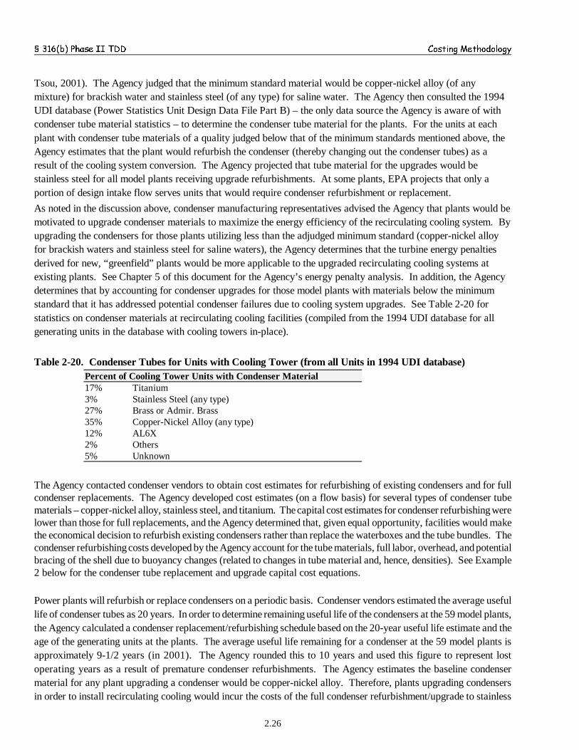
§ 316(b) Phase II TDD Costing Methodology
2.26
Tsou, 2001). The Agency judged that the minimum standard material would be copper-nickel alloy (of anymixture) for brackish water and stainless steel (of any type) for saline water. The Agency then consulted the 1994UDI database (Power Statistics Unit Design Data File Part B) – the only data source the Agency is aware of withcondenser tube material statistics – to determine the condenser tube material for the plants. For the units at eachplant with condenser tube materials of a quality judged below that of the minimum standards mentioned above, theAgency estimates that the plant would refurbish the condenser (thereby changing out the condenser tubes) as aresult of the cooling system conversion. The Agency projected that tube material for the upgrades would bestainless steel for all model plants receiving upgrade refurbishments. At some plants, EPA projects that only aportion of design intake flow serves units that would require condenser refurbishment or replacement.
As noted in the discussion above, condenser manufacturing representatives advised the Agency that plants would bemotivated to upgrade condenser materials to maximize the energy efficiency of the recirculating cooling system. Byupgrading the condensers for those plants utilizing less than the adjudged minimum standard (copper-nickel alloyfor brackish waters and stainless steel for saline waters), the Agency determines that the turbine energy penaltiesderived for new, “greenfield” plants would be more applicable to the upgraded recirculating cooling systems atexisting plants. See Chapter 5 of this document for the Agency’s energy penalty analysis. In addition, the Agencydetermines that by accounting for condenser upgrades for those model plants with materials below the minimumstandard that it has addressed potential condenser failures due to cooling system upgrades. See Table 2-20 forstatistics on condenser materials at recirculating cooling facilities (compiled from the 1994 UDI database for allgenerating units in the database with cooling towers in-place).
Table 2-20. Condenser Tubes for Units with Cooling Tower (from all Units in 1994 UDI database)Percent of Cooling Tower Units with Condenser Material17% Titanium3% Stainless Steel (any type)27% Brass or Admir. Brass35% Copper-Nickel Alloy (any type)12% AL6X2% Others5% Unknown
The Agency contacted condenser vendors to obtain cost estimates for refurbishing of existing condensers and for fullcondenser replacements. The Agency developed cost estimates (on a flow basis) for several types of condenser tubematerials – copper-nickel alloy, stainless steel, and titanium. The capital cost estimates for condenser refurbishing werelower than those for full replacements, and the Agency determined that, given equal opportunity, facilities would makethe economical decision to refurbish existing condensers rather than replace the waterboxes and the tube bundles. Thecondenser refurbishing costs developed by the Agency account for the tube materials, full labor, overhead, and potentialbracing of the shell due to buoyancy changes (related to changes in tube material and, hence, densities). See Example2 below for the condenser tube replacement and upgrade capital cost equations.
Power plants will refurbish or replace condensers on a periodic basis. Condenser vendors estimated the average usefullife of condenser tubes as 20 years. In order to determine remaining useful life of the condensers at the 59 model plants,the Agency calculated a condenser replacement/refurbishing schedule based on the 20-year useful life estimate and theage of the generating units at the plants. The average useful life remaining for a condenser at the 59 model plants isapproximately 9-1/2 years (in 2001). The Agency rounded this to 10 years and used this figure to represent lostoperating years as a result of premature condenser refurbishments. The Agency estimates the baseline condensermaterial for any plant upgrading a condenser would be copper-nickel alloy. Therefore, plants upgrading condensersin order to install recirculating cooling would incur the costs of the full condenser refurbishment/upgrade to stainless
§ 316(b) Phase II TDD Costing Methodology
2.27
steel, less the 10 years of useful life already expended, on average, in a condenser made of a lesser material (e.g.,copper-nickel alloy). The economic analysis then uses these capital cost estimates in the calculation of net annualizedcosts. See the EBA. As explained in the EBA, the full capital cost value of the replacement is reduced to represent lostoperating years of the existing condenser.
2.3 RECURRING ANNUAL COSTS OF POST-COMPLIANCE MONITORING
Existing facilities that fall within the scope of this proposed rule would be required to perform biological monitoringof impingement and entrainment, and visual or remote inspections of the cooling water intake structure and anyadditional technologies, on an on-going basis. Additional ambient water quality monitoring may also be required offacilities depending on the specifications of their NPDES permits. Facilities would be expected to analyze the resultsfrom their monitoring efforts and provide these results in an annual status report to the permitting authority. In addition,facilities would be required to maintain records of all submitted documents, supporting materials, and monitoring resultsfor at least three years. (Note that the Director may require that records be kept for a longer period to coincide withthe life of the NPDES permit.)
EPA expects that facility managers, biologists, biological technicians, statisticians, and clerical staff will devote timetoward gathering, preparing, submitting and maintaining records of the post-compliance monitoring information thatis required by the proposed rule. To develop representative profiles of each employee's relative contribution, EPAassumed burden estimates that reflect the staffing and expertise typically found in power generating plants. In doingthis, EPA considered the time and qualifications necessary to complete a variety of tasks: collecting, preparing, andanalyzing samples; enumerating organisms; performing statistical analyses; performing visual or remote inspectionsof installed technologies; compiling and submitting yearly status reports; and maintaining records of monitoring results.For each activity burden assumption, EPA selected time estimates to reflect the expected effort necessary to carry outthese activities under normal conditions and reasonable labor efficiency.
The costs to the respondent facilities associated with these time commitments can be estimated by multiplying the timespent in each labor category by an appropriately loaded hourly wage rate. All base wage rates used for facility laborcategories were derived from the Bureau of Labor Statistics (BLS) Occupational Handbook 2002-2003 (BLS, 2002).Additional detail on the development of cost estimates for annual post-compliance monitoring can be found in the DraftInformation Collection Request for Cooling Water Intake Structures Phase II Existing Facilities Proposed Rule.
EPA estimated the annual cost of post-compliance monitoring to be approximately $62,650 for freshwater facilities(i.e., facilities withdrawing cooling water from freshwater rivers and streams; or lakes and reservoirs), andapproximately $78,300 for marine facilities (i.e., facilities withdrawing cooling water from estuaries and tidal rivers;or oceans) and Great Lakes facilities.
2.4 ONE-TIME COSTS FOR TRACK II DEMONSTRATION STUDIES
Under the proposed rule, all facilities would submit a comprehensive demonstration study to characterize the sourcewater baseline in the vicinity of the intake, characterize the operation of the intake, and confirm that the technology(ies),operational measures and restoration measures proposed and/or implemented at the intake meet the applicableperformance standards. EPA developed burden and cost estimates for the comprehensive demonstration study in a
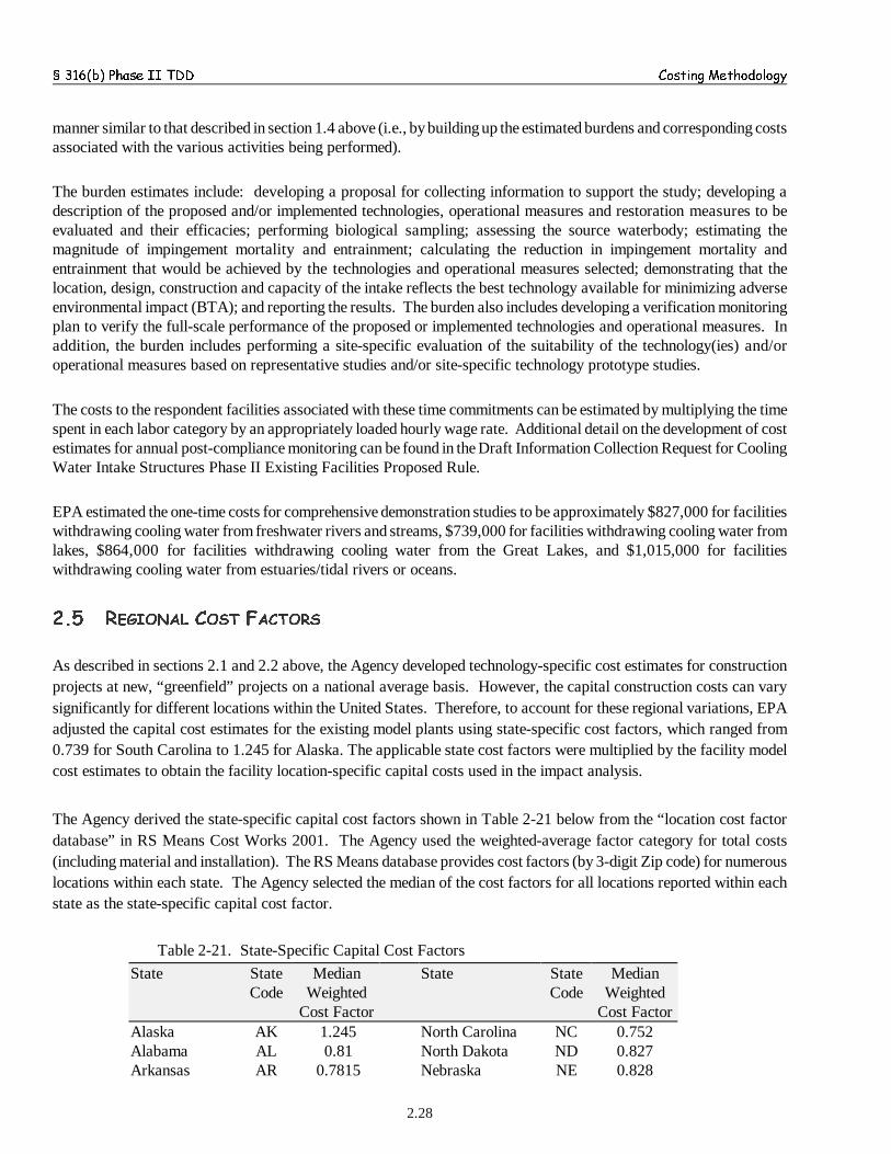
§ 316(b) Phase II TDD Costing Methodology
2.28
manner similar to that described in section 1.4 above (i.e., by building up the estimated burdens and corresponding costsassociated with the various activities being performed).
The burden estimates include: developing a proposal for collecting information to support the study; developing adescription of the proposed and/or implemented technologies, operational measures and restoration measures to beevaluated and their efficacies; performing biological sampling; assessing the source waterbody; estimating themagnitude of impingement mortality and entrainment; calculating the reduction in impingement mortality andentrainment that would be achieved by the technologies and operational measures selected; demonstrating that thelocation, design, construction and capacity of the intake reflects the best technology available for minimizing adverseenvironmental impact (BTA); and reporting the results. The burden also includes developing a verification monitoringplan to verify the full-scale performance of the proposed or implemented technologies and operational measures. Inaddition, the burden includes performing a site-specific evaluation of the suitability of the technology(ies) and/oroperational measures based on representative studies and/or site-specific technology prototype studies.
The costs to the respondent facilities associated with these time commitments can be estimated by multiplying the timespent in each labor category by an appropriately loaded hourly wage rate. Additional detail on the development of costestimates for annual post-compliance monitoring can be found in the Draft Information Collection Request for CoolingWater Intake Structures Phase II Existing Facilities Proposed Rule.
EPA estimated the one-time costs for comprehensive demonstration studies to be approximately $827,000 for facilitieswithdrawing cooling water from freshwater rivers and streams, $739,000 for facilities withdrawing cooling water fromlakes, $864,000 for facilities withdrawing cooling water from the Great Lakes, and $1,015,000 for facilitieswithdrawing cooling water from estuaries/tidal rivers or oceans.
2.5 REGIONAL COST FACTORS
As described in sections 2.1 and 2.2 above, the Agency developed technology-specific cost estimates for constructionprojects at new, “greenfield” projects on a national average basis. However, the capital construction costs can varysignificantly for different locations within the United States. Therefore, to account for these regional variations, EPAadjusted the capital cost estimates for the existing model plants using state-specific cost factors, which ranged from0.739 for South Carolina to 1.245 for Alaska. The applicable state cost factors were multiplied by the facility modelcost estimates to obtain the facility location-specific capital costs used in the impact analysis.
The Agency derived the state-specific capital cost factors shown in Table 2-21 below from the “location cost factordatabase” in RS Means Cost Works 2001. The Agency used the weighted-average factor category for total costs(including material and installation). The RS Means database provides cost factors (by 3-digit Zip code) for numerouslocations within each state. The Agency selected the median of the cost factors for all locations reported within eachstate as the state-specific capital cost factor.
Table 2-21. State-Specific Capital Cost Factors
State StateCode
MedianWeighted
Cost Factor
State StateCode
MedianWeighted
Cost FactorAlaska AK 1.245 North Carolina NC 0.752Alabama AL 0.81 North Dakota ND 0.827Arkansas AR 0.7815 Nebraska NE 0.828
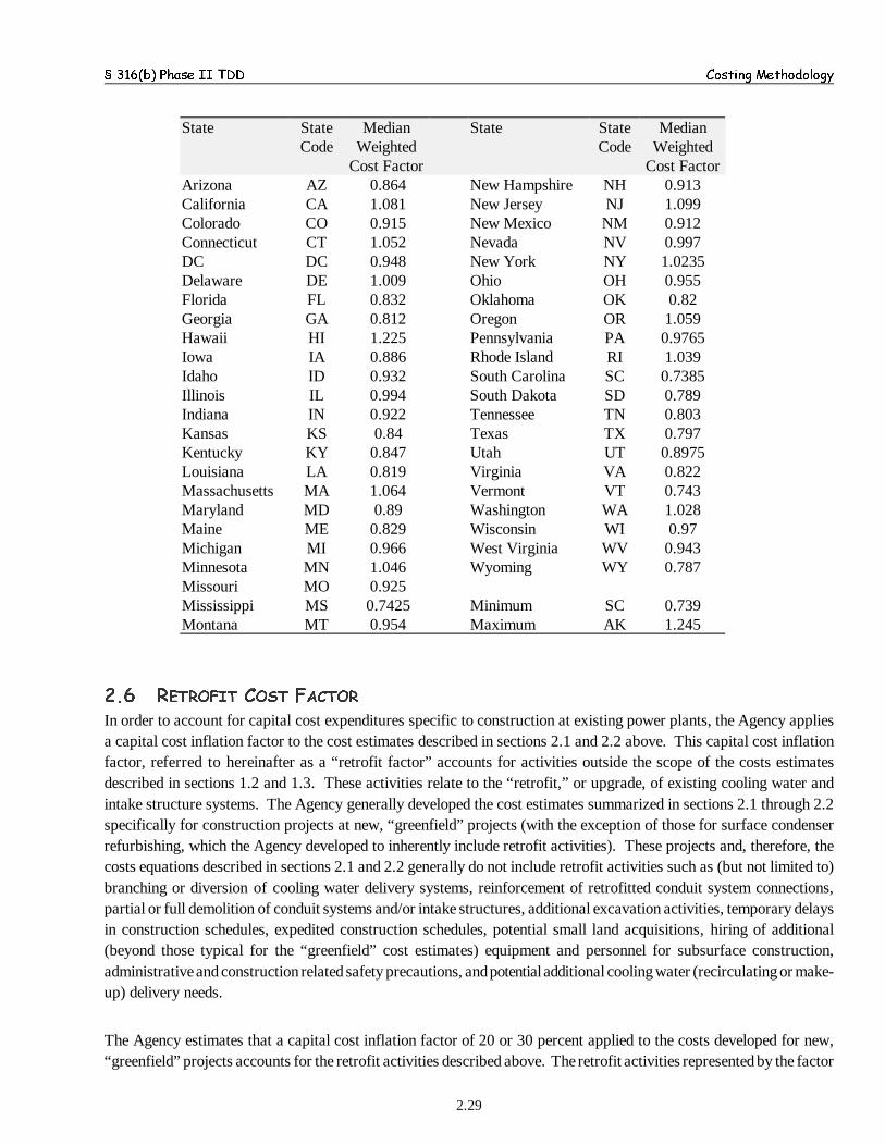
§ 316(b) Phase II TDD Costing Methodology
State StateCode
MedianWeighted
Cost Factor
State StateCode
MedianWeighted
Cost Factor
2.29
Arizona AZ 0.864 New Hampshire NH 0.913California CA 1.081 New Jersey NJ 1.099Colorado CO 0.915 New Mexico NM 0.912Connecticut CT 1.052 Nevada NV 0.997DC DC 0.948 New York NY 1.0235Delaware DE 1.009 Ohio OH 0.955Florida FL 0.832 Oklahoma OK 0.82Georgia GA 0.812 Oregon OR 1.059Hawaii HI 1.225 Pennsylvania PA 0.9765Iowa IA 0.886 Rhode Island RI 1.039Idaho ID 0.932 South Carolina SC 0.7385Illinois IL 0.994 South Dakota SD 0.789Indiana IN 0.922 Tennessee TN 0.803Kansas KS 0.84 Texas TX 0.797Kentucky KY 0.847 Utah UT 0.8975Louisiana LA 0.819 Virginia VA 0.822Massachusetts MA 1.064 Vermont VT 0.743Maryland MD 0.89 Washington WA 1.028Maine ME 0.829 Wisconsin WI 0.97Michigan MI 0.966 West Virginia WV 0.943Minnesota MN 1.046 Wyoming WY 0.787Missouri MO 0.925Mississippi MS 0.7425 Minimum SC 0.739Montana MT 0.954 Maximum AK 1.245
2.6 RETROFIT COST FACTOR
In order to account for capital cost expenditures specific to construction at existing power plants, the Agency appliesa capital cost inflation factor to the cost estimates described in sections 2.1 and 2.2 above. This capital cost inflationfactor, referred to hereinafter as a “retrofit factor” accounts for activities outside the scope of the costs estimatesdescribed in sections 1.2 and 1.3. These activities relate to the “retrofit,” or upgrade, of existing cooling water andintake structure systems. The Agency generally developed the cost estimates summarized in sections 2.1 through 2.2specifically for construction projects at new, “greenfield” projects (with the exception of those for surface condenserrefurbishing, which the Agency developed to inherently include retrofit activities). These projects and, therefore, thecosts equations described in sections 2.1 and 2.2 generally do not include retrofit activities such as (but not limited to)branching or diversion of cooling water delivery systems, reinforcement of retrofitted conduit system connections,partial or full demolition of conduit systems and/or intake structures, additional excavation activities, temporary delaysin construction schedules, expedited construction schedules, potential small land acquisitions, hiring of additional(beyond those typical for the “greenfield” cost estimates) equipment and personnel for subsurface construction,administrative and construction related safety precautions, and potential additional cooling water (recirculating or make-up) delivery needs.
The Agency estimates that a capital cost inflation factor of 20 or 30 percent applied to the costs developed for new,“greenfield” projects accounts for the retrofit activities described above. The retrofit activities represented by the factor
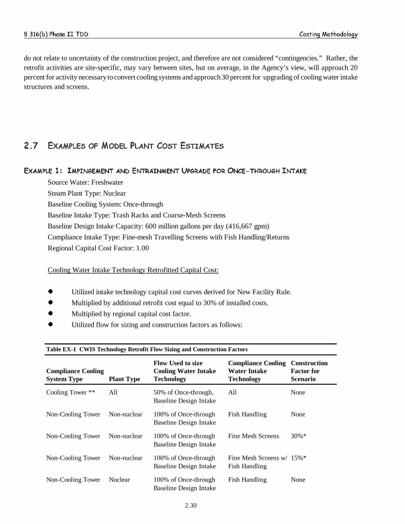
§ 316(b) Phase II TDD Costing Methodology
2.30
do not relate to uncertainty of the construction project, and therefore are not considered “contingencies.” Rather, theretrofit activities are site-specific, may vary between sites, but on average, in the Agency’s view, will approach 20percent for activity necessary to convert cooling systems and approach 30 percent for upgrading of cooling water intakestructures and screens.
2.7 EXAMPLES OF MODEL PLANT COST ESTIMATES
EXAMPLE 1: IMPINGEMENT AND ENTRAINMENT UPGRADE FOR ONCE-THROUGH INTAKE
Source Water: Freshwater
Steam Plant Type: Nuclear
Baseline Cooling System: Once-through
Baseline Intake Type: Trash Racks and Coarse-Mesh Screens
Baseline Design Intake Capacity: 600 million gallons per day (416,667 gpm)
Compliance Intake Type: Fine-mesh Travelling Screens with Fish Handling/Returns
Regional Capital Cost Factor: 1.00
Cooling Water Intake Technology Retrofitted Capital Cost:
! Utilized intake technology capital cost curves derived for New Facility Rule.
! Multiplied by additional retrofit cost equal to 30% of installed costs.
! Multiplied by regional capital cost factor.
! Utilized flow for sizing and construction factors as follows:
Table EX-1 CWIS Technology Retrofit Flow Sizing and Construction Factors
Compliance CoolingSystem Type Plant Type
Flow Used to sizeCooling Water IntakeTechnology
Compliance CoolingWater IntakeTechnology
ConstructionFactor forScenario
Cooling Tower ** All 50% of Once-through,Baseline Design Intake
All None
Non-Cooling Tower Non-nuclear 100% of Once-throughBaseline Design Intake
Fish Handling None
Non-Cooling Tower Non-nuclear 100% of Once-throughBaseline Design Intake
Fine Mesh Screens 30%*
Non-Cooling Tower Non-nuclear 100% of Once-throughBaseline Design Intake
Fine Mesh Screens w/Fish Handling
15%*
Non-Cooling Tower Nuclear 100% of Once-throughBaseline Design Intake
Fish Handling None
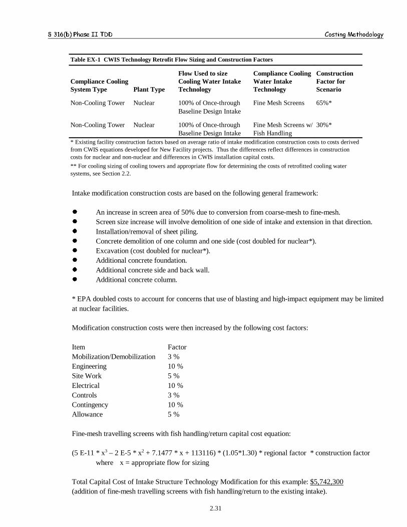
§ 316(b) Phase II TDD Costing Methodology
Table EX-1 CWIS Technology Retrofit Flow Sizing and Construction Factors
Compliance CoolingSystem Type Plant Type
Flow Used to sizeCooling Water IntakeTechnology
Compliance CoolingWater IntakeTechnology
ConstructionFactor forScenario
2.31
Non-Cooling Tower Nuclear 100% of Once-throughBaseline Design Intake
Fine Mesh Screens 65%*
Non-Cooling Tower Nuclear 100% of Once-throughBaseline Design Intake
Fine Mesh Screens w/Fish Handling
30%*
* Existing facility construction factors based on average ratio of intake modification construction costs to costs derivedfrom CWIS equations developed for New Facility projects. Thus the differences reflect differences in constructioncosts for nuclear and non-nuclear and differences in CWIS installation capital costs.
** For cooling sizing of cooling towers and appropriate flow for determining the costs of retrofitted cooling watersystems, see Section 2.2.
Intake modification construction costs are based on the following general framework:
! An increase in screen area of 50% due to conversion from coarse-mesh to fine-mesh.! Screen size increase will involve demolition of one side of intake and extension in that direction.! Installation/removal of sheet piling.! Concrete demolition of one column and one side (cost doubled for nuclear*).! Excavation (cost doubled for nuclear*).! Additional concrete foundation.! Additional concrete side and back wall.! Additional concrete column.
* EPA doubled costs to account for concerns that use of blasting and high-impact equipment may be limitedat nuclear facilities.
Modification construction costs were then increased by the following cost factors:
Item FactorMobilization/Demobilization 3 %Engineering 10 %Site Work 5 %Electrical 10 %Controls 3 %Contingency 10 %Allowance 5 %
Fine-mesh travelling screens with fish handling/return capital cost equation:
(5 E-11 * x3 – 2 E-5 * x2 + 7.1477 * x + 113116) * (1.05*1.30) * regional factor * construction factorwhere x = appropriate flow for sizing
Total Capital Cost of Intake Structure Technology Modification for this example: $5,742,300 (addition of fine-mesh travelling screens with fish handling/return to the existing intake).
§ 316(b) Phase II TDD Costing Methodology
2.32
Total Capital Cost of Intake Upgrade: $5,742,300.
Cooling Water Intake Technology O&M Costs:
Based on outreach with industry representatives, EPA estimated annual O&M cost as a percentage of totalcapital cost (that is, those costs developed for new facility projects, not including retrofit factors). The O&Mcost factor ranges between 8 percent of total capital cost for the smallest size traveling screens with and withoutfish handling equipment and 5 percent for the largest traveling screen since O&M costs do not increaseproportionately with screen size. The screen O&M costs are based on the size of the screen, which are basedon the initial sizing flow. For this example, the Agency uses the sizing flow of full, baseline once-through flow.
O&M Equation for Fine-mesh Travelling Screens with Fish Handling/Return: -3 E-13 * x3 – 4 E-8 * x2 + 0.2081 * x + 11485
Cooling Water Intake Technology O&M Costs for This Example: $69,548
Total Annual O&M Costs for this Example: $69,548
EXAMPLE 2: COOLING SYSTEM CONVERSION
Source Water: Estuary / Tidal RiverSteam Plant Type: Fossil Baseline Cooling System: Once-throughBaseline Intake Type: Trash Racks and Coarse-Mesh ScreensBaseline Design Intake Capacity: 600 million gallons per day (416,667 gpm)Converted Cooling System: Mechanical-Draft Wet Cooling TowersCompliance Intake Type: Fine-mesh Travelling Screens with Fish Handling/ReturnsReduced Intake Capacity: 33,333 gpm (416,667 gpm * 0.08)Regional Capital Cost Factor: 1.08
Recirculating Wet Cooling Tower Cost Development:
Cooling Tower Material of Construction: RedwoodNumber of Cooling Tower Units: 2Cooling Flow for Each Tower Unit: 208,334 gpm
Basic Redwood Tower with Splash Fill Capital Cost Equation:
n * (-5E-5 * x2 + 70.271 * x + 25393) * regional factor,where x = cooling flow per unit n = number of cooling units
Items included in the installed tower capital cost equation:

§ 316(b) Phase II TDD Costing Methodology
5 The Agency excluded makeup water pump costs from its derived equations for cooling systemconversions. In doing so, the Agency attempted to compensate for the situations where existing pumpscan be reused in the converted recirculating system, as was the case for the Jefferies Steam Plantconversion (see Chapter 4 for futher discussion of cooling tower conversion example cases). However, theAgency recognized that the probability of existing circulating water pumps being reused for retrofittedtower systems was low. Therefore, because the Agency was able to confirm the reuse of existing intakestructures for three of the example cases, the Agency considered the cost of the makeup pump to offset thepossible savings of pump reuse such as the Jefferies plant to be appropriate. The Agency estimates thatthe installed cost of intake pumps, such as for the model plant cost example above, would be a very smallfraction of the total cost of the installed cooling tower system (less than 0.25 percent). For the final rule’sanalyses, the Agency will consider the costs of new intake pumps at a portion, or all cooling systemconversions.
2.33
- Wet tower, furnished & erectedincludes internal tower piping, risers, and valvesincludes splash fillincludes fans and motorsincludes electrical service and housing
- Site preparation, clearing, grading - Excavation for basins and piping- Circulating water piping, valves, and fittings to and from condenser- Access roads- Full circulating pumps and housing- Installed concrete basins, sumps, and footings- Electrical wiring, controls, and transformers - Blowdown-water treatment facility - Acceptance testing - Installation
Factors included in the installed tower capital cost equation (i.e., these factors inflate the direct capital costs):
- Construction management, mobilization and demobilization- Design engineering and architectural fees- Contractor overhead and profit- Turnkey Fee- Contingencies
Additional Cooling Tower Retrofit Scaling Factor: 20 percent.Regional Capital Cost Factor: 1.08
Total Capital Cost of Installed Cooling Tower (2 unit tower system): $44,550,000 (new facility project cost)+ $8,910,000 (retrofit cost factor) = $53,550,000
Intake and Discharge Piping Modification Capital Costs:
Pipe modification costs are based on the following assumptions:5
! Piping material and installation cost is $12 per in-diameter per ft-length.
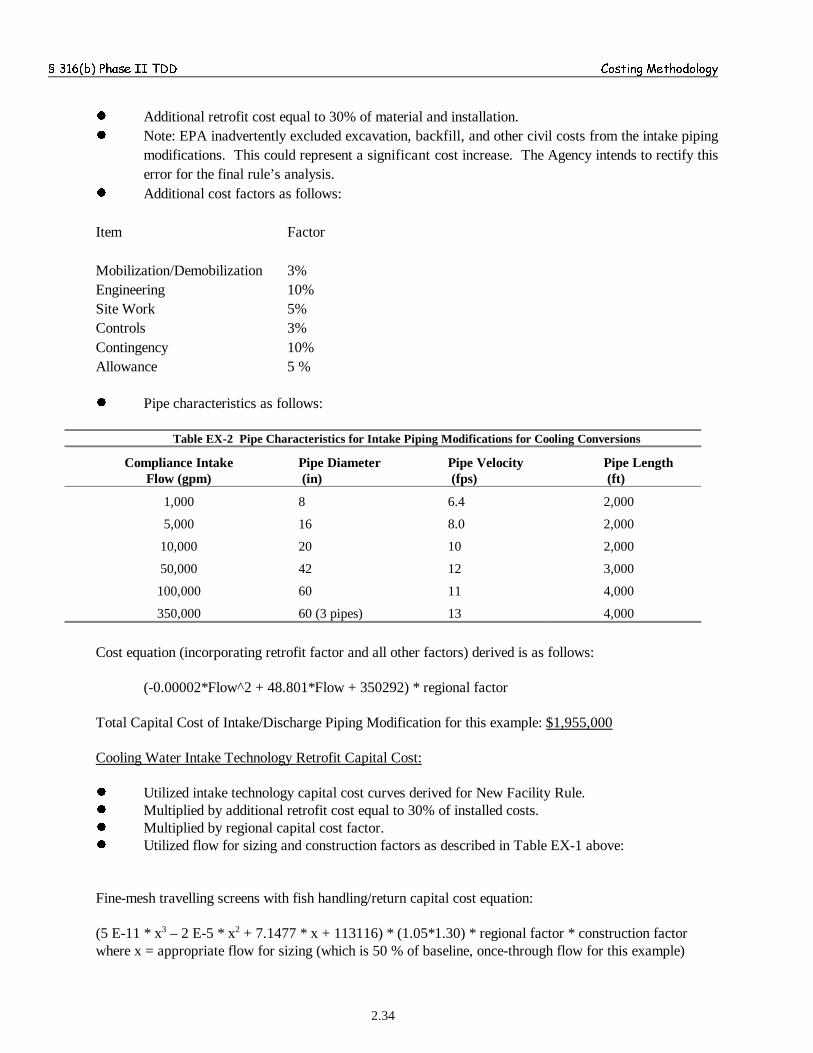
§ 316(b) Phase II TDD Costing Methodology
2.34
! Additional retrofit cost equal to 30% of material and installation.! Note: EPA inadvertently excluded excavation, backfill, and other civil costs from the intake piping
modifications. This could represent a significant cost increase. The Agency intends to rectify thiserror for the final rule’s analysis.
! Additional cost factors as follows:
Item Factor
Mobilization/Demobilization 3%Engineering 10%Site Work 5%Controls 3%Contingency 10%Allowance 5 %
! Pipe characteristics as follows:
Table EX-2 Pipe Characteristics for Intake Piping Modifications for Cooling Conversions
Compliance IntakeFlow (gpm)
Pipe Diameter (in)
Pipe Velocity (fps)
Pipe Length (ft)
1,000 8 6.4 2,000
5,000 16 8.0 2,000
10,000 20 10 2,000
50,000 42 12 3,000
100,000 60 11 4,000
350,000 60 (3 pipes) 13 4,000
Cost equation (incorporating retrofit factor and all other factors) derived is as follows:
(-0.00002*Flow^2 + 48.801*Flow + 350292) * regional factor
Total Capital Cost of Intake/Discharge Piping Modification for this example: $1,955,000
Cooling Water Intake Technology Retrofit Capital Cost:
! Utilized intake technology capital cost curves derived for New Facility Rule.! Multiplied by additional retrofit cost equal to 30% of installed costs.! Multiplied by regional capital cost factor.! Utilized flow for sizing and construction factors as described in Table EX-1 above:
Fine-mesh travelling screens with fish handling/return capital cost equation:
(5 E-11 * x3 – 2 E-5 * x2 + 7.1477 * x + 113116) * (1.05*1.30) * regional factor * construction factorwhere x = appropriate flow for sizing (which is 50 % of baseline, once-through flow for this example)
§ 316(b) Phase II TDD Costing Methodology
2.35
Total Capital Cost of Intake Structure Technology Modification for this example: $1,748,800 (this includesaddition of fine mesh travelling screens with fish handling/return to the existing intake).
Total Capital Cost of Cooling System Conversion and Intake Upgrade: $57,414,400.
Condenser Upgrade Capital Costs:
EPA estimates that some condensers would require upgrades premature to the end of their useful lives due tothe cooling system conversion. For this example case, the condenser baseline tube material is Copper/NickelAlloy. The Agency determined that the tubes would be upgraded to 304 Stainless Steel for a cooling towerusing brackish cooling water. This upgrade would occur when the existing condenser had 10 years of usefullife remaining. Therefore, EPA developed cost estimates for the tube upgrade and the tube replacement.
The Capital Cost equation for CuNi replacement is as follows:
Number of Cooling Tower Units * (18.046 * Unit Cooling Flow – 13134) * Regional Factor.
! Accounts for cost of materials! Accounts for vibration/stability analysis! Accounts for labor, overhead, etc.! EPA utilizes a 1.58 factor for safety at nuclear plants! Replacement tubing includes non-corroding internal tubing liner! Does not include an additional retrofit or allowance, due to the fact that the cost estimates forming the
basis of the curves were for actual tube replacement projects.
Capital Cost of Existing Material Condenser Tube Replacement: $8,029,400
Capital Cost of Condenser Tube Upgrade: $8,774,600
The economic analysis calculates the net capital cost to the facility for the premature replacement ofthe condenser tube sheets. The analysis accounts for the upgraded material and deducts the useful lifeof the replacement. See the Economic and Benefits Analysis for more information.
Operation and Maintenance Costs of Baseline Intake Pumping (once-through):
- Pumping head estimated at 50 ft for all systems.- Pump and motor efficiency estimated at 70 percent.- Annual hours of operation estimated at 7860 (i.e., 90 percent of 8760).- Energy cost estimated at $0.03/KWh. This value is set near the average wholesale cost of electricity.
To be conservative, this estimation of the unit energy cost is intended to account for the pumpingelectricity costs and does not account for such O&M costs as pump maintenance.
Baseline Intake Pumping Annual Cost Equation: - (50 * Flow * 8.33 * 0.746 * 7860 * 0.03) / (33,000* 0.7)
Baseline Intake Annual Pumping Cost in this Example: $1,321,500
Wet Cooling Tower Operation and Maintenance:
- Includes periodic equipment replacement and maintenance costs (i.e., 10th and 20th year overhauls).

§ 316(b) Phase II TDD Costing Methodology
2.36
- Includes pumping and fanning O&M requirements.- Includes blowdown-water treatment and disposal.- Accounts for increase in equipment replacement costs as tower useful life diminishes.- Includes chemical addition.- Does not include turbine efficiency penalty, which is factored into the economic analysis through lost
revenue.
Redwood Wet Tower O&M Equation: n * (-4E-6 * x2 +11.617 * x + 2055.2)Where x = cooling flow per unit
n = number of cooling units
Wet Cooling Tower O&M Cost Estimate for this Example: $4,497,300
Intake Pumping O&M Costs:
Developed in a manner very similar to the once-through, baseline intake pumping costs. However, thecompliance intake flow is used in place of the baseline, once-through flow.
Wet Tower Compliance Intake Pumping O&M Cost Estimate for this Example: $105,700
Cooling Water Intake Technology O&M Costs:
Based on outreach with industry representatives, EPA estimated annual O&M cost as a percentageof total capital cost (that is, those costs developed for new facility projects, not including retrofitfactors). The O&M cost factor ranges between 8 percent of total capital cost for the smallest sizetraveling screens with and without fish handling equipment and 5 percent for the largest travelingscreen since O&M costs do not increase proportionately with screen size. The screen O&M costs arebased on the size of the screen, which are based on the initial sizing flow. For this example, theAgency uses the sizing flow of ½ of the baseline once-through flow.
O&M Equation for Fine-mesh Travelling Screens with Fish Handling/Return: -3 E-13 * x3 – 4 E-8 * x2 + 0.2081 * x + 11485
Cooling Water Intake Technology O&M Costs for This Example: $50,390
Total Annual O&M Costs for this Example: $3,331,900
2.9 REPOWERING FACILITIES AND MODEL PLANT COSTS
Under this proposed rule certain forms of repowering could be undertaken by an existing power generating facility thatuses a cooling water intake structure and it would remain subject to regulation as a Phase II existing facility. Forexample, the following scenarios would be existing facilities under the proposed rule:
- An existing power generating facility undergoes a modification of its processshort of total replacement of the process and concurrently increases the designcapacity of its existing cooling water intake structures;
- An existing power generating facility builds a new process for purposes of the

§ 316(b) Phase II TDD Costing Methodology
2.37
same industrial operation and concurrently increases the design capacity of itsexisting cooling water intake structures;
- An existing power generating facility completely rebuilds its process but uses theexisting cooling water intake structure with no increase in design capacity.
Thus, in most situations, repowering an existing power generating facility would beaddressed under this proposed rule.
As discussed in Section III.B of the preamble, the section 316(b) Survey acquired technological and economicinformation from facilities for the years 1998 and 1999. With this information, the Agency established a subset offacilities potentially subject to this rule. Since 1999, some existing facilities have proposed and/or enacted changes totheir facilities in the form of repowering that could potentially affect the applicability of this proposal or a facility’scompliance costs. The Agency therefore conducted research into repowering facilities for the section 316(b) existingfacility rule and any information available on proposed changes to their cooling water intake structures. The Agencyused two separate databases to assemble available information for the repowering facilities: RDI’s NEWGen Database,November 2001 version and the Section 316(b) Survey.
In January 2000, EPA conducted a survey of the technological and economic characteristics of 961 steam-electricgenerating plants. Only the detailed questionnaire, filled out by 283 utility plants and 50 nonutility plants, containsinformation on planned changes to the facilities’ cooling systems (Part 2, Section E). Of the respondents to the detailedquestionnaire, only six facilities (three utility plants and three nonutility plants) indicated that their future plans wouldlead to changes in the operation of their cooling water intake structures
The NEWGen database is a compilation of detailed information on new electric generating capacity proposed over thenext several years. The database differentiates between proposed capacity at new (greenfield) facilities andadditions/modifications to existing facilities. To identify repowering facilities of interest, the Agency screened the 1,530facilities in the NEWGen database with respect to the following criteria: facility status, country, and steam electricadditions. The Agency then identified 124 NEWGen facilities as potential repowering facilities.
Because the NEWGen database provides more information on repowering than the section 316(b) survey, the Agencyused it as the starting point for the analysis of repowering facilities. Of the 124 NEWGen facilities identified asrepowering facilities, 85 responded to the section 316(b) survey. Of these 85 facilities, 65 are in-scope and 20 are outof scope of this proposal. For each of the 65 in scope facilities, the NEWGen database provided an estimation of thetype and extent of the capacity additions. The Agency found that 36 of the 65 facilities would be combined-cyclefacilities after the repowering changes. Of these, 34 facilities are projected to decrease their cooling water intake afterrepowering (through the conversion from a simple steam cycle to a combined-cycle plant). The other 31 facilities withinthe scope of the rule would increase their cooling water intake. The Agency examined the characteristics of thesefacilities projected to undergo repowering and determined the waterbody type from which they withdraw cooling water.The results of this analysis are presented in Table 2-22.
Table 2-22 - In-scope Existing Facilities Projected to Enact Repowering Changes
§ 316(b) Phase II TDD Costing Methodology
2.38
Waterbody Type Repowering Facilities Projected toIncrease Cooling Water
Withdrawals
Repowering Facilities Projected toDecrease or Maintain Cooling Water
Withdrawals
Ocean N/A N/A
Estuary/Tidal River 3 17
Freshwater River/Stream 14 10
Freshwater Lake/Reservoir 10 1
Great Lake 0 1
Of the 65 in scope facilities identified as repowering facilities in the NEWGen database, 24 received the detailedquestionnaire, which requested information about planned cooling water intake structures and changes to capacity.Nineteen of these 24 facilities are utilities and the remaining five are nonutilities. The Agency analyzed the section316(b) detailed questionnaire data for these 24 facilities to identify facilities that indicated planned modifications to theircooling systems which will change the capacity of intake water collected for the plant and the estimated cost to complywith today’s proposal. Four such facilities were identified, two utilities and two nonutilities. Both utilities respondedthat the planned modifications will decrease their cooling water intake capacity and that they do not have any plannedcooling water intake structures that will directly withdraw cooling water from surface water. The two nonutilities, onthe other hand, indicated that the planned modifications will increase their cooling water intake capacity and that theydo have planned cooling water intake structures that will directly withdraw cooling water from surface water.
Using the NEWGen and section 316(b) detailed questionnaire information on repowering facilities, the Agencyexamined the extent to which planned and/or enacted repowering changes would effect cooling water withdrawals and,therefore, the potential costs of compliance with this proposal. Because the Agency developed a cost estimatingmethodology that primarily utilizes design intake flow as the independent variable, the Agency examined the extent towhich compliance costs would change if the repowering data summarized above were incorporated into the cost analysisof this rule. The Agency determined that projected compliance costs for facilities withdrawing from estuaries could belower after incorporating the repowering changes. The primary reason for this is the fact that the majority of estuaryrepowering facilities would change from a steam cycle to a combined-cycle, thereby maintaining or decreasing theircooling water withdrawals (note that a combined-cycle facility generally will withdraw one-third of the cooling waterof a comparably sized full-steam facility). Therefore, the portion of compliance costs for regulatory options thatincluded flow reduction requirements or technologies could significantly decrease if the Agency incorporated repoweringchanges into the analysis. As shown in Table 2-22 the majority of facilities projected to increase cooling waterwithdrawals due to the repowering changes use freshwater sources. In turn, the compliance costs for these facilitieswould increase if the Agency incorporated repowering for this proposal.
2.9 CAPACITY UTILIZATION RATE CUT-OFF
The Agency is proposing standards for reducing impingement mortality but not entrainment when a facility operatesat a capacity utilization rate of less than 15 percent over the course of several years (see § 125.94 (b)(2) of the proposedrule). Capacity utilization rate means the ratio between the average annual net generation of the facility (in MWh) andthe total net capability of the facility (in MW) multiplied by the number of available hours during a year. The averageannual generation is to be measured over a five year period (if available) of representative operating conditions.Incorporation of capacity utilization into the level of control was found to be the most economically practicable given
§ 316(b) Phase II TDD Costing Methodology
2.39
these facilities’ reduced operating levels. Fifteen percent capacity utilization corresponds to facility operation forroughly 55 days in a year (that is, less than two months). The Agency refers to this differentiation between facilitiesbased on their operating time as a capacity utilization cut-off. Facilities operating at capacity utilization rates of lessthan 15 percent are generally facilities of significant age, including the oldest facilities within the scope of the rule.Frequently, entities will refer to these facilities as peaker plants, though the definition extends to a broader range offacilities. These peaker plants are less efficient and more costly to operate than other facilities. Therefore, operatingcompanies generally utilize them only when demand is highest and, therefore, economic conditions are favorable.Because these facilities operate only a fraction of the time compared to other facilities, such as base-load plants, thepeaking plants achieve sizable flow reductions over their maximum design annual intake flows. The lower the intakeflow at a site, the lesser the potential for entraining of organisms. Therefore, the concept of an entrainment reductionrequirement for such facilities does not appear necessary. Additionally, the plants typically operate during two specificperiods: the extreme winter and the extreme summer demand periods. Each of these periods can, in some cases,coincide with periods of abundant aquatic concentrations and/or sensitive spawning events. However, it is generallyaccepted that peak winter and summer periods will not be the most crucial for aquatic organism communities on anational basis.
Based on an analysis of data collected through the detailed industry questionnaire and the short technical questionnaire,EPA believes that today’s proposed rule would apply to 539 existing steam electric power generating facilities. Of these,53 facilities operate at less than 15 percent capacity utilization and would potentially only comply with impingementcontrols, with 34 of these estimated to actually require such controls. (The remaining 19 facilities have existingimpingement controls).
Of the facilities exceeding the capacity utilization cut-off, the median and average capacity utilization is 50 percent.As a general rule, steam plants operate cyclically between 100 percent load and standby. In turn, the intake flow rateof a typical steam plant cycles between flows approaching the full design rate and standby (that is, near-zero intakeflow). Facilities operating with an average capacity utilization of 50 percent would generally withdraw more than threetimes as much water over the course of time than a facility with a capacity utilization of less than 15. Therefore, thecapacity utilization cut-off coincides with an approximate flow reduction, and hence entrainment reduction, of roughly70 percent as compared to the average facility above the cut-off. This level of reduction is within the range ofperformance standards for entrainment reduction. Were the Agency to establish the cut-off at less than 20 percentcapacity utilization, an additional 18 facilities would be subject to the reduced requirements and the comparable flowreduction would be roughly 60 percent. The operating period would extend to approximately 75 days (that is, 2.5months) for the hypothetical 20 percent cut-off. Were the Agency to establish the cut-off at less than 25 percentcapacity, 108 of the 539 facilities would be subject to the reduced standards, and the comparable entrainment reductionwould be roughly 54 percent. For a hypothetical 25 percent capacity utilization cut-off, the operating period wouldextend to approximately three months.
The median age of generating units with capacity utilization factors less than 15 percent is 48 years in 2002. Themedian age of generating units with capacity utilization factors of less than 25 percent and equal to or greater than 15percent is 43 years. The age of generating units shows a continued trend upwards as capacity utilization rate increases.This trend agrees with the theory that existing peaking plants generally are aged facilities only dispatched wheneconomic conditions are favorable and/or demand is highest.
The Agency examined the cooling water use of all plants for trends associated with or related to capacity utilization.As the analysis of unit age described above shows, most plants with low capacity utilization rates are very old. Theseplants generally utilize once-through cooling systems. For some plants, not all generating units may be available orcapable of operating during extended periods, and the plant may staggered operation of generating units may beemployed. However, as discussed above, the Agency believes that these aged units generally operate at or near peakcapacity when they are dispatched. Therefore, the intake pumps will operate at near design intake capacity whenfunctioning. Because a peaker plant will only operate for limited times during the year, its overall use of water (that

§ 3
16(b
) Ph
ase I
I T
DD
Cos
ting
Meth
odol
ogy
2.40
is, t
he a
vera
ge a
nnua
l int
ake)
wou
ld b
e si
gnif
ican
tly b
elow
its
desi
gn m
axim
um in
take
rat
e.
The
Age
ncy
calc
ulat
ed a
rat
io o
f ac
tual
ann
ual i
ntak
e (f
or 1
998)
to m
axim
um-d
esig
n an
nual
inta
ke f
or t
he p
lant
s w
ithin
the
sco
pe o
f th
is r
ule
and
com
pare
d th
is t
o ca
paci
ty u
tiliz
atio
n.
Tho
ugh
the
data
sho
ws
a si
gnif
ican
tde
gree
of
scat
ter,
the
Age
ncy
conc
lude
s th
at t
he d
ata
plot
ted
in F
igur
e 2-
1 (a
ctua
l-to
-des
ign
inta
ke r
atio
ver
sus
capa
city
util
izat
ion
rate
for
all
mod
el p
lant
sw
ithin
sco
pe o
f th
is p
ropo
sed
rule
) sh
ows
that
gen
eral
ly, t
he lo
wer
the
cap
acity
util
izat
ion
of a
pla
nt, t
he lo
wer
the
inta
ke f
low
as
a pe
rcen
t of
the
max
imum
desi
gn in
take
cap
abili
ty.
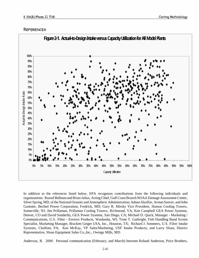
§ 316(b) Phase II TDD Costing Methodology
2.41
Figure 2-1. Actual-to-Design Intake versus Capacity Utilization for All Model Plants
0%
5%
10%
15%
20%
25%
30%
35%
40%
45%
50%
55%
60%
65%
70%
75%
80%
85%
90%
95%
100%
0% 5% 10% 15% 20% 25% 30% 35% 40% 45% 50% 55% 60% 65% 70% 75% 80% 85% 90% 95% 100%
Capacity Utilization
Actu
al-to
-Des
ign
Inta
ke R
atio
REFERENCES
In addition to the references listed below, EPA recognizes contributions from the following individuals andorganizations: Russel Bellman and Brian Julius, Acting Chief, Gulf Coast Branch NOAA Damage Assessment Center,Silver Spring, MD, of the National Oceanic and Atmospheric Administration; Adnan Alsaffar, Arman Sanver, and JohnGantnier, Bechtel Power Corporation, Fredrick, MD; Gary R. Mirsky Vice President, Hamon Cooling Towers,Somerville, NJ; Jim Prillaman, Prillaman Cooling Towers, Richmond, VA; Ken Campbell GEA Power Systems,Denver, CO and David Sanderlin, GEA Power Systems, San Diego, CA; Michael D. Quick, Manager - Marketing /Communications, U.S. Filter - Envirex Products, Waukesha, WI; Trent T. Gathright, Fish Handling Band ScreenSpecialist, Marketing Manager, Brackett Geiger USA, Inc., Houston, TX; Richard J. Sommers, U.S. Filter IntakeSystems, Chalfont, PA; Ken McKay, VP Sales/Marketing, USF Intake Products; and Larry Sloan, DistrictRepresentative, Sloan Equipment Sales Co.,Inc., Owings Mills, MD.
Anderson, R. 2000. Personal communication (February, and March) between Roland Anderson, Price Brothers,

§ 316(b) Phase II TDD Costing Methodology
2.42
Dayton, OH and Faysal Bekdash, SAIC.
Antaya, Bill. 1999. Personal communication between Bill Antaya, The Coon-De Visser Company and Faysal Bekdash,SAIC.
Boles, D.E., et al. 1973. Technical and Economic Evaluations of Cooling Systems Blowdown Control Techniques.
Burns, J.M., and Micheletti, W.C. Comparison of Wet and Dry Cooling Systems for Combined Cycle Power Plants.November 4, 2000.
Burns, J.M. and Tsou, J.L., 2001. Modular Steam Condenser Replacements Using Corrosion Resistant HighPerformance Stainless Steel Tubing. Proceedings from a conference of the American Society of Mechanical Engineers.
Campbell, Thomas A. 2001. Correspondence from Thomas A. Campbell, Managing Partner, Campbell, George &Strong, LLP, to the Cooling Water Intake Structure (New Facilities) Proposed Rule Comment Docket Clerk, WaterDocket, EPA. Subject: Submission of Comments Regarding May 25, 2001 Federal Register Notice of DataAvailability; National Pollutant Discharge Elimination System–Regulations Addressing Cooling Water IntakeStructures for New Facilities. June 25, 2001.Coss, Tim. 2000. Personal communication (February, and March) between Tim Coss, the Boulder Trenchless Groupand Faysal Bekdash, SAIC.
U.S. Department of Energy (DOE). 1994. Environmental Mitigation at Hydroelectric Projects: Volume II. Benefitsand Costs of Fish Passage and Protection. Francfort, J.E., Cada, G.F., Dauble, D.D., Hunt, R.T., Jones, D.W.,Rinehart, B.N., Sommers, G.L. Costello, R.J. Idaho National Engineering Laboratory.
U.S. EPA. Economic and Engineering Analyses of the Proposed §316(b) New Facility Rule. Office of Water.August 2000. EPA
U.S. EPA (EPA). (1996). Technology Transfer Handbook - Management of Water Treatment Plant Residuals,EPA/625/R-95/008, April 1996.
Edison Electric Institute (EEI). Environmental Directory of U.S. Power Plants. 1996.
Electric Power Research Institute (EPRI). 1995. Proceedings: Cooling Tower and Advanced Cooling SystemsConference. Summary of Report TR-104867, obtained from EPRI’s Web site at http://www.epri.com on 12/1/99.
EPRI. 1986a. Performance of a Capacitive Cooling System for Dry Cooling. Summary of Report CS-4322, obtainedfrom EPRI’s Web site at http://www.epri.com on 12/1/99.
EPRI. 1986b. Wet-Dry Cooling Demonstration: Test Results. Summary of Report CS-4321, obtained from EPRI’sWeb site at http://www.epri.com on 12/1/99.
Federal Energy Regulatory Commission (FERC). 1995. Preliminary Assessment of Fish Entrainment at HydropowerProjects, A Report on Studies and Protective Measures, Volume 1. Office of Hydropower Licensing, Washington, DC.Paper No. DPR-10.
Flory, A. FlowServe Pump Division. Telephone Contact with John Sunda, SAIC. Regarding equipment costs for intakepumps and variable frequency drives. May 14, 2001.
Ganas, Michael. Assembling underwater concrete pipelines. Published article provided by Price Brothers (no date or

§ 316(b) Phase II TDD Costing Methodology
2.43
journal name).
GEA Power Cooling Systems, Inc. (GEA). Undated. Direct Air Cooled Condenser Installations. Brochure. R-227.
Gerwick, B.C. Jr. 2000. Construction of Marine And offshore structures. 2nd edition. CRC Press.
Gunderboom, Inc. System Specification: Gunderboom Marine/Aquatic Life Exclusion System, obtained from theGunderboom, Inc. Web site at http://www.gunderboom.com/specs/MLES/MLEST1.htm.
Hensley, J.C. Undated. Cooling Tower Fundamentals. 2nd Edition. The Marley Cooling Tower Company (Mission,Kansas). 1985.
Huber, Gary. 2000. Personal communication (February, and March) between Gary Huber, Permalok and FaysalBekdash, SAIC.
Kaplan, Charles. Memo to Martha Segall. April 18, 2000. Subject: Flow Reduction. (Water Docket #1-1073-TC).
Mirsky, G.R., et al. 1992. The Latest Worldwide Technology in Environmentally Designed Cooling Towers. CoolingTower Institute 1992 Annual Meeting Technical Paper Number TP92-02.
Mirsky, G. and Bautier, J. 1997. Designs for Cooling Towers and Air Cooled Steam Conensers that Meet Today’sStringent Environmental Requirements. Presented at the EPRI 1997 Cooling Tower Conference (St. Petersburg,Florida) and ASME 1997 Joint Power Conference (Denver, Colorado).
Mirsky, G. 2000. Personal communication between Gary Mirsky, Hamon Cooling Towers and Faysal Bekdash, SAIC.Email dated 3/27/00.
Montdardon, S. 2000. Personal communication (February, and March) between Stephan Montdardon, Torch Inc. andFaysal Bekdash, SAIC.
Nicholson, J.M. (Stone & Webster Engineering Corp.) 1993. Preliminary Engineering Evaluation. Public ServiceElectric and Gas Company Salem Generating Station, NJPDES Permit No. NJ0005622, Public Hearing.
Congress of the United States, Office of Technology Assessment (OTA). 1995. Fish Passage Technologies: Protectionat Hydropower Facilities. OTA-ENV-641.
Paroby, Rich. 1999. Personal communication between Rich Paroby, District Sales Manager, Water Process Groupand Deborah Nagle, U.S. EPA. E-mail dated May 12, 1999.
Power Plant Research Program (PPRP) for Maryland. 1999. Cumulative Environmental Impact Report (CEIR), 10thAnnual. Obtained from Maryland’s PPRP Web site at http://www.dnr.md.us/bay/pprp/ on 11/18/99.
R.S. Means Company, Inc. (R.S. Means). 1997a. Plumbing Cost Data 1998. 21st Annual Edition.
R.S. Means. 1997b. Heavy Construction Cost Data 1998. 12th Annual Edition.
R.S. Means. 1997c. Environmental Remediation Cost Data 1998.
Science Applications International Corporation (SAIC). 1994. Background Paper Number 3: Cooling Water IntakeTechnologies. Prepared by SAIC for U.S. EPA. Washington, DC.

§ 316(b) Phase II TDD Costing Methodology
2.44
SAIC. 1996. Supplement to Background Paper 3: Cooling Water Intake Technologies. Prepared by SAIC for U.S.EPA. Washington, DC.
SAIC. 2000. Cost Research and Analysis of Cooling Water Technologies for 316(b) Regulatory Options, Preparedby SAIC for Tetra Tech, for U.S. EPA. Washington, DC.
Stone & Webster Engineering Corporation. 1992. Evaluation of the Potential Costs and Environmental Impacts ofRetrofitting Cooling Towers on Existing Steam Electric Power Plants that Have Obtained Variances Under Section316(a) of the Clean Water Act. Prepared by Stone & Webster for the Edison Electric Institute (EEI).
Tallon, B. GEA Power Systems Inc. Telephone Contact with John Sunda, SAIC. Regarding Air Cooled CondenserFans. October 22, 2001.
Tatar, G. El Dorado Energy. Telephone Contact with John Sunda, SAIC. Regarding operation of the air cooledcondenser fans. October 19, 2001.
Taylor, S. Bechtel. Telephone Contact with John Sunda, SAIC. Regarding cooling water pumping and condenseroperation. May 11, 2001.
US Filter/Johnson Screens (US Filter). 1998. Surface Water Intake Screen Technical Data. Brochure.
Utility Data Institute (UDI). 1995. EEI Power Statistics Database. Prepared by UDI for EEI. Washington, DC.
The Utility Water Action Group (UWAG). 1978. Thermal Control Cost Factors. Chapter 2 - Report on the CapitalCosts of Closed-Cycle Cooling Systems. Prepared by Stone & Webster Engineering Corporation for UWAG.
Additional References Used for General Information But Not Specifically Cited
Envirex Inc. 1973. Traveling screens to protect fish in water intake systems. Bulletin No. 316-300.
Gathright, Trent. 1999. Personal communication between Trent Gathright, Marketing Manager, Brackett Greenand Faysal Bekdash, SAIC. Letter dated November 16, 1999.GEA. Undated. PAC SystemTM: The Parallel Condensing System. Brochure.
Geiger. Undated. Geiger Fipro - Fimat. Efficient, modern fish protection systems. Fish repelling plants of thenew generation. Brochure.
Norell, Bob. 1999. Personal communication between Bob Norell, US Filter/Johnson Screens and Tracy Scriba,SAIC.
Puder, M.G. and J.A. Veil. 1999. Summary Data on Cooling Water Use at Utilities and Nonutilities. Preparedby Puder and Veil, Argonne National Laboratory for U.S. DOE.
Swanekamp, Robert, PE. 1998. Parallel condensing combines best of all-wet, all-dry methods. Power.July/August 1998 issue.
U.S. Filter. 1999. Raw Water Screening Intake Systems. Brochure.
§ 316(b) Phase II TDD Costing Methodology
2.45
List of Cost Curves and Equations in Appendix B
Chart 2-1. Capital Costs of Basic Cooling Towers with Various Building Material (Delta 10 Degrees)Chart 2-2. Douglas Fir Cooling Tower Capital Costs with Various Features (Delta 10 Degrees)Chart 2-3. Red Wood Cooling Tower Capital Costs with Various Features (Delta 10 Degrees)Chart 2-4. Concrete Cooling Tower Capital Costs with Various Features (Delta 10 Degrees)Chart 2-5. Steel Cooling Tower Capital Costs with Various Features (Delta 10 Degrees)Chart 2-6. Fiberglass Cooling Tower Capital Costs with Various Features (Delta 10 Degrees)Chart 2-7. Actual Capital Costs for Wet Cooling Tower Projects and Comparable Costs from EPA Cost
CurvesChart 2-8. Total O&M Red Wood Tower Annual Costs - 1st ScenarioChart 2-9. Total O&M Concrete Tower Annual Costs - 1st ScenarioChart 2-10. Variable Speed Pump Capital CostsChart 2-11. Municipal Water Use CostsChart 2-12. Gray Water Use CostsChart 2-13. Capital Costs of Passive Screens Based on Well DepthChart 2-14. Capital Costs of Passive Screens for a Flow Velocity 0.5 ft/secChart 2-15. Capital Costs of Passive Screens for a Flow Velocity 1 ft/secChart 2-16. Velocity Cap Total Capital CostsChart 2-17. Concrete Fittings for Intake Flow Velocity ReductionChart 2-18. Steel Fittings for Intake Flow Velocity ReductionChart 2-19. Traveling Screens Capital Cost Without Fish Handling Features Flow Velocity 0.5 ft/secChart 2-20. Traveling Screens Capital Cost With Fish Handling Features Flow Velocity 0.5 ft/secChart 2-21. Traveling Screens Capital Cost Without Fish Handling Features Flow Velocity 1 ft/secChart 2-22. Traveling Screens Capital Cost With Fish Handling Features Flow Velocity 1 ft/secChart 2-23. Fish Spray Pumps Capital CostsChart 2-24. O&M Costs for Traveling Screens Without Fish Handling Features Flow Velocity 0.5 ft/secChart 2-25. O&M Costs for Traveling Screens With Fish Handling Features Flow Velocity 0.5 ft/secChart 2-26. O&M Costs for Traveling Screens Without Fish Handling Features Flow Velocity 1 ft/secChart 2-27. O&M Costs for Traveling Screens With Fish Handling Features Flow Velocity 1 ft/secChart 2-28. Capital Cost of Fish Handling Equipment Screen Flow Velocity 0.5 ft/secChart 2-29. O&M for Fish Handling Features Flow Velocity 0.5 ft/secChart 2-30. Gunderboom Capital and O&M Costs for Simple Floating Structure
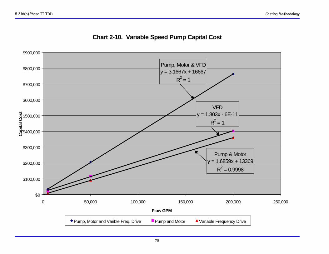
§ 316(b) Phase II TDD Costing Methodology
70
Chart 2-10. Variable Speed Pump Capital Cost
Pump, Motor & VFDy = 3.1667x + 16667
R2 = 1
Pump & Motory = 1.6859x + 13369
R2 = 0.9998
VFDy = 1.803x - 6E-11
R2 = 1
$0
$100,000
$200,000
$300,000
$400,000
$500,000
$600,000
$700,000
$800,000
$900,000
0 50,000 100,000 150,000 200,000 250,000
Flow GPM
Cap
ital C
ost
Pump, Motor and Varible Freq. Drive Pump and Motor Variable Frequency Drive
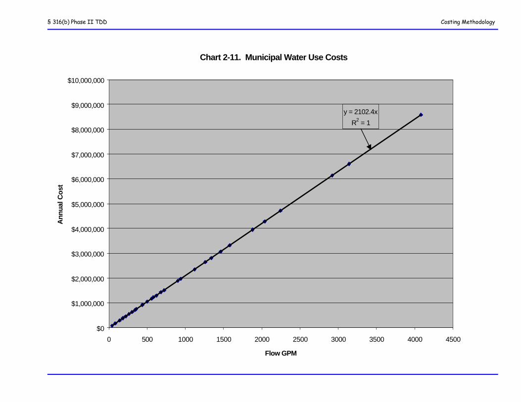
§ 316(b) Phase II TDD Costing Methodology
Chart 2-11. Municipal Water Use Costs
y = 2102.4x
R2 = 1
$0
$1,000,000
$2,000,000
$3,000,000
$4,000,000
$5,000,000
$6,000,000
$7,000,000
$8,000,000
$9,000,000
$10,000,000
0 500 1000 1500 2000 2500 3000 3500 4000 4500
Flow GPM
An
nu
al C
ost
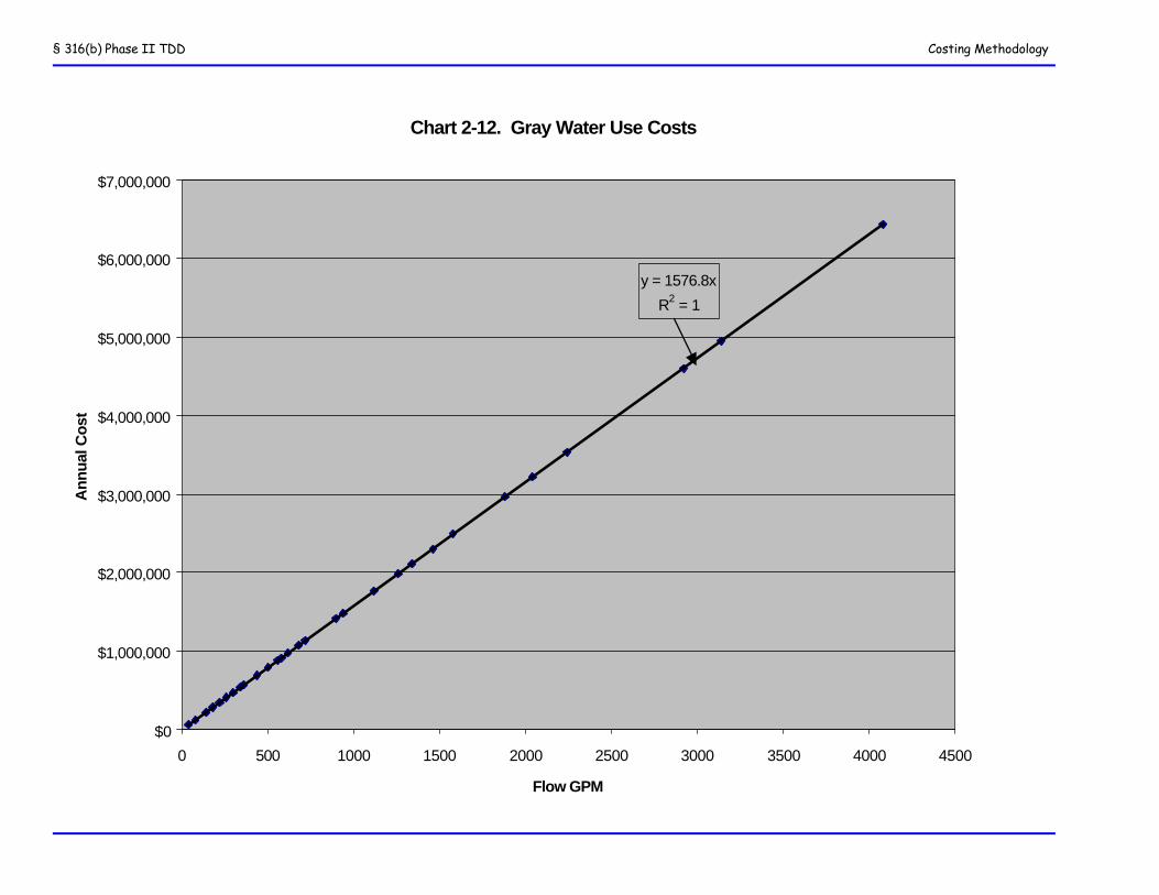
§ 316(b) Phase II TDD Costing Methodology
Chart 2-12. Gray Water Use Costs
y = 1576.8x
R2 = 1
$0
$1,000,000
$2,000,000
$3,000,000
$4,000,000
$5,000,000
$6,000,000
$7,000,000
0 500 1000 1500 2000 2500 3000 3500 4000 4500
Flow GPM
An
nu
al C
ost
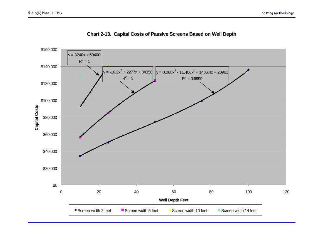
§ 316(b) Phse II TDD Costing Methodology
Chart 2-13. Capital Costs of Passive Screens Based on Well Depth
y = 0.088x3 - 11.406x2 + 1406.4x + 20961
R2 = 0.9999
y = -10.2x2 + 2277x + 34350
R2 = 1
y = 3240x + 59400
R2 = 1
$0
$20,000
$40,000
$60,000
$80,000
$100,000
$120,000
$140,000
$160,000
0 20 40 60 80 100 120
Well Depth Feet
Cap
ital C
ost
s
Screen width 2 feet Screen width 5 feet Screen width 10 feet Screen width 14 feet
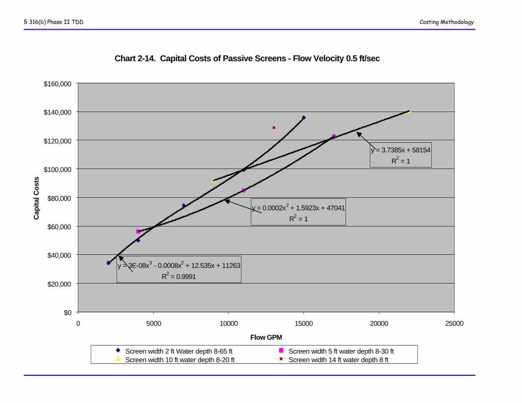
§ 316(b) Phase II TDD Costing Methodology
Chart 2-14. Capital Costs of Passive Screens - Flow Velocity 0.5 ft/sec
y = 3E-08x3 - 0.0008x2 + 12.535x + 11263
R2 = 0.9991
y = 0.0002x2 + 1.5923x + 47041
R2 = 1
y = 3.7385x + 58154
R2 = 1
$0
$20,000
$40,000
$60,000
$80,000
$100,000
$120,000
$140,000
$160,000
0 5000 10000 15000 20000 25000
Flow GPM
Cap
ital C
ost
s
Screen width 2 ft Water depth 8-65 ft Screen width 5 ft water depth 8-30 ftScreen width 10 ft water depth 8-20 ft Screen width 14 ft water depth 8 ft
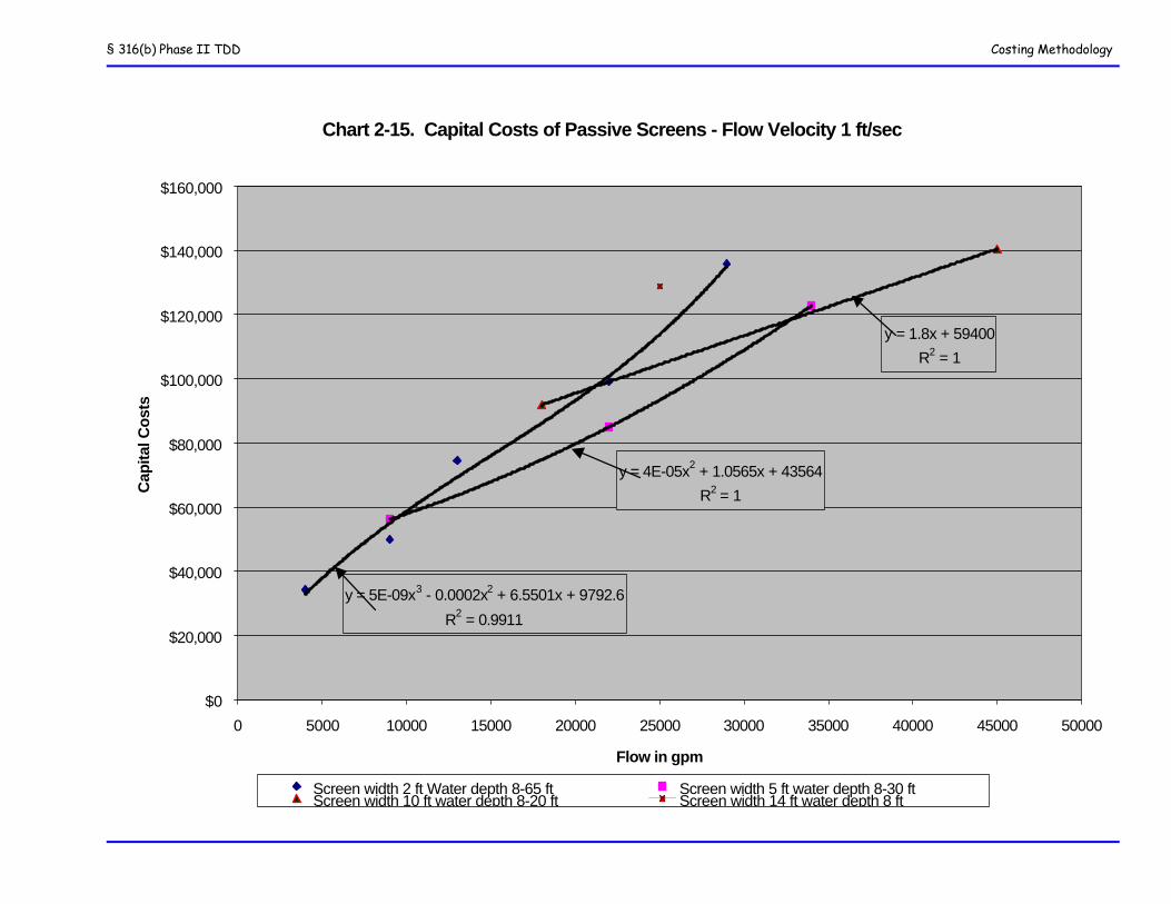
§ 316(b) Phase II TDD Costing Methodology
Chart 2-15. Capital Costs of Passive Screens - Flow Velocity 1 ft/sec
y = 4E-05x2 + 1.0565x + 43564
R2 = 1
y = 1.8x + 59400
R2 = 1
y = 5E-09x3 - 0.0002x2 + 6.5501x + 9792.6
R2 = 0.9911
$0
$20,000
$40,000
$60,000
$80,000
$100,000
$120,000
$140,000
$160,000
0 5000 10000 15000 20000 25000 30000 35000 40000 45000 50000
Flow in gpm
Cap
ital C
ost
s
Screen width 2 ft Water depth 8-65 ft Screen width 5 ft water depth 8-30 ftScreen width 10 ft water depth 8-20 ft Screen width 14 ft water depth 8 ftPoly. (Screen width 2 ft Water depth 8-65 ft)
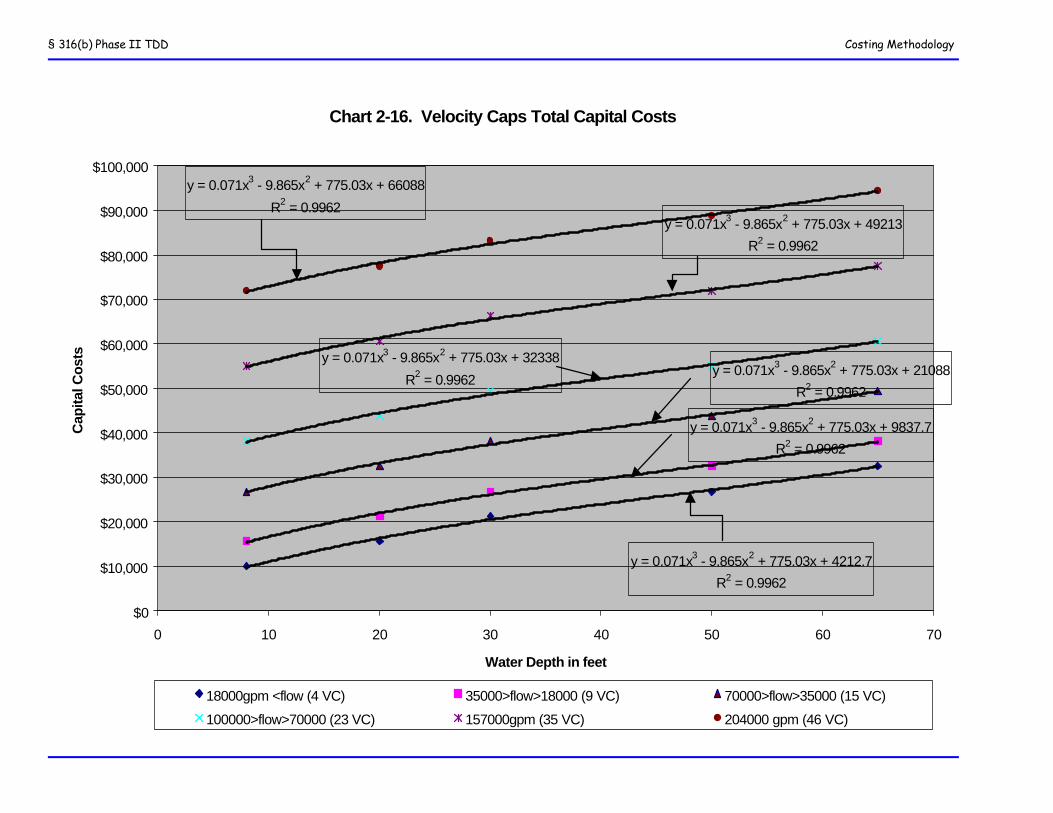
§ 316(b) Phase II TDD Costing Methodology
Chart 2-16. Velocity Caps Total Capital Costs
y = 0.071x3 - 9.865x2 + 775.03x + 4212.7
R2 = 0.9962
y = 0.071x3 - 9.865x2 + 775.03x + 32338
R2 = 0.9962
y = 0.071x3 - 9.865x2 + 775.03x + 49213
R2 = 0.9962
y = 0.071x3 - 9.865x2 + 775.03x + 66088
R2 = 0.9962
y = 0.071x3 - 9.865x2 + 775.03x + 21088
R2 = 0.9962
y = 0.071x3 - 9.865x2 + 775.03x + 9837.7
R2 = 0.9962
$0
$10,000
$20,000
$30,000
$40,000
$50,000
$60,000
$70,000
$80,000
$90,000
$100,000
0 10 20 30 40 50 60 70
Water Depth in feet
Cap
ital C
ost
s
18000gpm <flow (4 VC) 35000>flow>18000 (9 VC) 70000>flow>35000 (15 VC)
100000>flow>70000 (23 VC) 157000gpm (35 VC) 204000 gpm (46 VC)
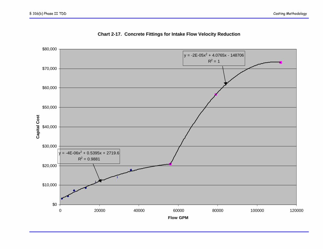
§ 316(b) Phase II TDD Costing Methodology
Chart 2-17. Concrete Fittings for Intake Flow Velocity Reduction
y = -4E-06x2 + 0.5395x + 2719.6R2 = 0.9881
y = -2E-05x2 + 4.0765x - 148706R2 = 1
$0
$10,000
$20,000
$30,000
$40,000
$50,000
$60,000
$70,000
$80,000
0 20000 40000 60000 80000 100000 120000
Flow GPM
Cap
ital
Co
st
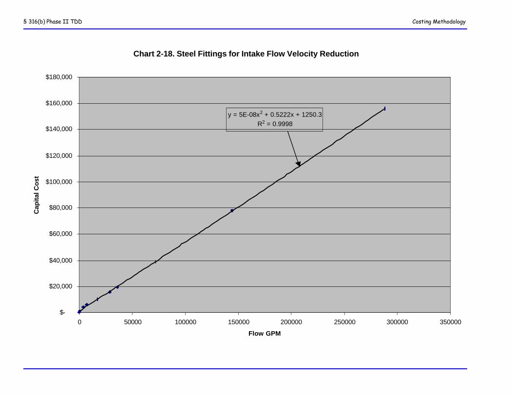
§ 316(b) Phase II TDD Costing Methodology
Chart 2-18. Steel Fittings for Intake Flow Velocity Reduction
y = 5E-08x2 + 0.5222x + 1250.3R2 = 0.9998
$-
$20,000
$40,000
$60,000
$80,000
$100,000
$120,000
$140,000
$160,000
$180,000
0 50000 100000 150000 200000 250000 300000 350000
Flow GPM
Cap
ital
Co
st
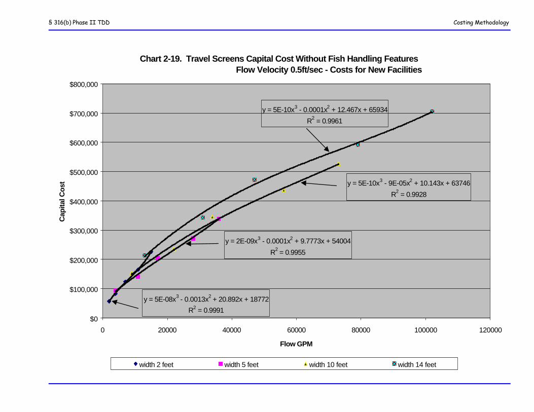
§ 316(b) Phase II TDD Costing Methodology
Chart 2-19. Travel Screens Capital Cost Without Fish Handling Features Flow Velocity 0.5ft/sec - Costs for New Facilities
y = 5E-10x3 - 0.0001x2 + 12.467x + 65934
R2 = 0.9961
y = 5E-10x3 - 9E-05x2 + 10.143x + 63746
R2 = 0.9928
y = 2E-09x3 - 0.0001x2 + 9.7773x + 54004
R2 = 0.9955
y = 5E-08x3 - 0.0013x2 + 20.892x + 18772
R2 = 0.9991$0
$100,000
$200,000
$300,000
$400,000
$500,000
$600,000
$700,000
$800,000
0 20000 40000 60000 80000 100000 120000
Flow GPM
Cap
ital C
ost
width 2 feet width 5 feet width 10 feet width 14 feet
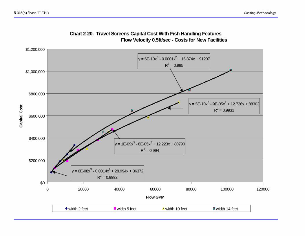
§ 316(b) Phase II TDD Costing Methodology
Chart 2-20. Travel Screens Capital Cost With Fish Handling Features Flow Velocity 0.5ft/sec - Costs for New Facilities
y = 6E-10x3 - 0.0001x2 + 15.874x + 91207
R2 = 0.995
y = 5E-10x3 - 9E-05x2 + 12.726x + 88302
R2 = 0.9931
y = 1E-09x3 - 8E-05x2 + 12.223x + 80790
R2 = 0.994
y = 6E-08x3 - 0.0014x2 + 28.994x + 36372
R2 = 0.9992$0
$200,000
$400,000
$600,000
$800,000
$1,000,000
$1,200,000
0 20000 40000 60000 80000 100000 120000
Flow GPM
Cap
ital C
ost
width 2 feet width 5 feet width 10 feet width 14 feet
§ 316(b) Phase II TDD Costing Methodology
Chart 2-21. Travel Screens Capital Cost Without Fish Handling Features Flow Velocity 1 ft/sec - Costs for New Facilities
y = 5E-11x3 - 2E-05x2 + 5.6762x + 81695
R2 = 0.9952
y = 5E-11x3 - 2E-05x2 + 5.0073x + 64193
R2 = 0.9902
y = 3E-10x3 - 4E-05x2 + 5.481x + 44997
R2 = 0.9962
y = 8E-09x3 - 0.0004x2 + 10.917x + 16321
R2 = 0.9911$0
$100,000
$200,000
$300,000
$400,000
$500,000
$600,000
$700,000
$800,000
0 50000 100000 150000 200000 250000
Flow GPM
Cap
ital C
ost
width 2 feet width 5 feet width 10 feet width 14 feet
§ 316(b) Phse II TDD Costing Methodology
Chart 2-22. Travel Screens Capital Cost With Fish Handling Features Flow Velocity 1 ft/sec - Costs for New Facilities
y = 5E-11x3 - 2E-05x2 + 7.1477x + 113116
R2 = 0.9942
y = 5E-11x3 - 2E-05x2 + 6.2849x + 88783
R2 = 0.9906
y = 2E-10x3 - 3E-05x2 + 6.921x + 68688
R2 = 0.9948
y = 8E-09x3 - 0.0004x2 + 15.03x + 33044
R2 = 0.9909
0
200000
400000
600000
800000
1000000
1200000
0 50000 100000 150000 200000 250000
Flow GPM
Cap
ital C
ost
width 2 feet width 5 feet width 10 feet width 14 feet
§ 316(b) Phase II TDD Costing Methodology
Chart 2-23. Fish Spray Pumps Capital Costs - Costs for New Facilities
y = -0.2394x2 + 47.9x + 364.04
R2 = 0.9907
y = 2E-06x3 - 0.0035x2 + 3.8696x + 2446.8
R2 = 1
$0
$1,000
$2,000
$3,000
$4,000
$5,000
$6,000
$7,000
$8,000
$9,000
$10,000
0 500 1000 1500 2000 2500
Flow GPM
Co
sts
of
Pu
mp
s In
stal
led
Spray pumps flow in GPM
§ 316(b) Phase II TDD Costing Methodology
Chart 2-24. O&M Cost for Traveling Screens Without Fish Handling Features Flow Velocity 0.5ft/sec
y = -2E-05x2 + 1.0121x + 2392.4
R2 = 0.9965
y = -7E-06x2 + 0.6204x + 4045.7
R2 = 0.9956
y = 9E-11x3 - 1E-05x2 + 0.8216x + 1319.5
R2 = 0.9997
y = 8E-12x3 - 2E-06x2 + 0.3899x + 7836.7
R2 = 0.9922
$0
$5,000
$10,000
$15,000
$20,000
$25,000
$30,000
$35,000
$40,000
0 20000 40000 60000 80000 100000 120000
Flow GPM
O&
M C
ost
s
Screen width 2 feet Screen width 5 feet Screen width 10 feet Screen width 14 feet
§ 316(b) Phase II TDD Costing Methodology
Chart 2-25. O&M Cost for Traveling Screens With Fish Handling Features Flow Velocity 0.5ft/sec
y = -3E-05x2 + 1.6179x + 3739.1R2 = 0.9943
y = 5E-12x3 - 1E-06x2 + 0.4835x + 10593R2 = 0.9912
y = -2E-06x2 + 0.5703x + 5864.4R2 = 0.9907
y = -1E-05x2 + 0.8563x + 5686.3R2 = 0.9943
$0
$10,000
$20,000
$30,000
$40,000
$50,000
$60,000
0 20000 40000 60000 80000 100000 120000
Flow GPM
O&
M C
ost
s
Screen Width 2 ft Screen Width 5 ft Screen Width 10 ft Screen Width 14 ft
§ 316(b) Phase II TDD Costing Methodology
Chart 2-26. O&M Cost for Traveling Screens Without Fish Handling Features Flow Velocity 1 ft/sec
y = -4E-06x2 + 0.5035x + 2334
R2 = 0.9853
y = -2E-06x2 + 0.3312x + 3621.1
R2 = 0.9963
y = 1E-11x3 - 3E-06x2 + 0.4047x + 1359.4
R2 = 1
y = 4E-13x3 - 3E-07x2 + 0.1715x + 8472.1
R2 = 0.9913
$0
$5,000
$10,000
$15,000
$20,000
$25,000
$30,000
$35,000
$40,000
0 50000 100000 150000 200000 250000
Flow GPM
O&
M C
ost
s
Screen width 2 feet Screen width 5 feet Screen width 10 feet Screen width 14 feet
§ 316(b) Phase II TDD Costing Methodology
Chart 2-27. O&M Cost for Traveling Screens With Fish Handling Features Flow Velocity 1 ft/sec
y = -8E-06x2 + 0.806x + 3646.7R2 = 0.982
y = -3E-13x3 - 4E-08x2 + 0.2081x + 11485R2 = 0.9903
y = -6E-07x2 + 0.2895x + 5705.3R2 = 0.9915
y = -3E-06x2 + 0.4585x + 5080.7R2 = 0.9954
$0
$10,000
$20,000
$30,000
$40,000
$50,000
$60,000
0 50000 100000 150000 200000 250000Flow GPM
O&
M C
ost
s
Screen Width 2 ft Screen Width 5 ft Screen Width 10 ft Screen Width 14 ft
§ 316(b) Phase II TDD Costing Methodology
Chart 2-28. Capital Cost of Fish Handling Equipment Screen Flow Velocity 0.5 ft/sec - Costs for New Facilities
y = 7E-11x3 - 2E-05x2 + 4.0881x + 30327
R2 = 0.9924
y = 3E-11x3 - 7E-06x2 + 3.0998x + 29468
R2 = 0.9939
y = -8E-10x3 + 5E-05x2 + 2.9353x + 32144
R2 = 0.9896
y = 4E-09x3 - 0.0002x2 + 9.7217x + 21120
R2 = 0.9994$0
$50,000
$100,000
$150,000
$200,000
$250,000
$300,000
$350,000
$400,000
0 20000 40000 60000 80000 100000 120000
Flow GPM
Cap
ital C
ost
width 2 feet width 5 feet width 10 feet width 14 feet
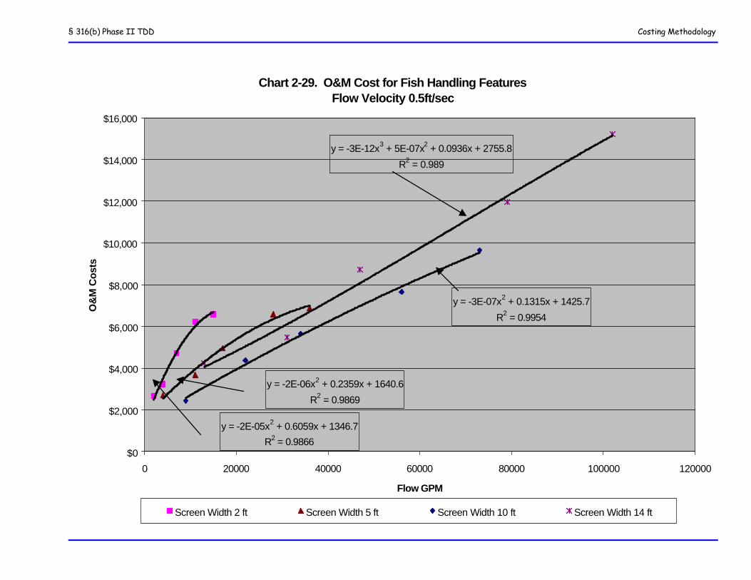
§ 316(b) Phase II TDD Costing Methodology
Chart 2-29. O&M Cost for Fish Handling Features Flow Velocity 0.5ft/sec
y = -2E-05x2 + 0.6059x + 1346.7
R2 = 0.9866
y = -3E-12x3 + 5E-07x2 + 0.0936x + 2755.8
R2 = 0.989
y = -3E-07x2 + 0.1315x + 1425.7
R2 = 0.9954
y = -2E-06x2 + 0.2359x + 1640.6
R2 = 0.9869
$0
$2,000
$4,000
$6,000
$8,000
$10,000
$12,000
$14,000
$16,000
0 20000 40000 60000 80000 100000 120000
Flow GPM
O&
M C
ost
s
Screen Width 2 ft Screen Width 5 ft Screen Width 10 ft Screen Width 14 ft
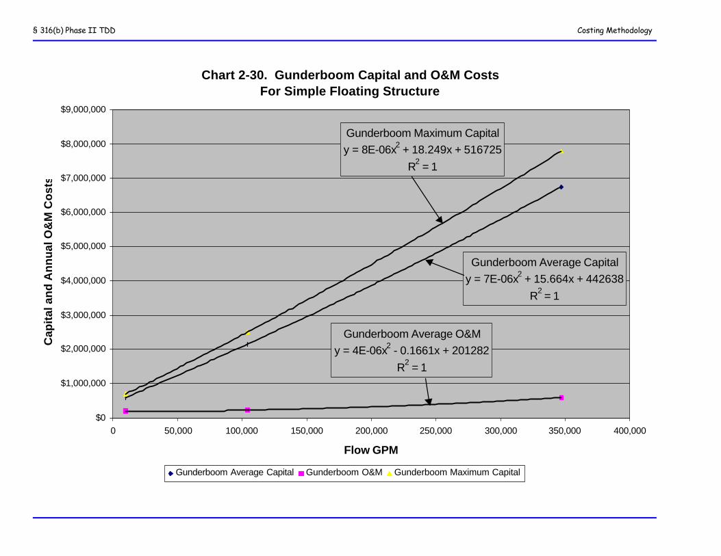
§ 316(b) Phase II TDD Costing Methodology
Chart 2-30. Gunderboom Capital and O&M CostsFor Simple Floating Structure
Gunderboom Average Capitaly = 7E-06x2 + 15.664x + 442638
R2 = 1
Gunderboom Average O&My = 4E-06x2 - 0.1661x + 201282
R2 = 1
Gunderboom Maximum Capitaly = 8E-06x2 + 18.249x + 516725
R2 = 1
$0
$1,000,000
$2,000,000
$3,000,000
$4,000,000
$5,000,000
$6,000,000
$7,000,000
$8,000,000
$9,000,000
0 50,000 100,000 150,000 200,000 250,000 300,000 350,000 400,000
Flow GPM
Cap
ital
an
d A
nn
ual
O&
M C
ost
s
Gunderboom Average Capital Gunderboom O&M Gunderboom Maximum Capital
Section 316(b) Phase II TDD Efficacy of Cooling Water Intake Structure Technologies
3 - 1
Chapter 3: Efficacy of Cooling Water
Intake Structure Technologies
INTRODUCTION
To support the Section 316(b) proposed rule for existing facilities, the Agency compiled data on the performance ofthe range of technologies currently used to minimize impingement and entrainment (I&E) at power plants nationwide.The goal of this data collection and analysis effort has been to determine whether specific technologies can bedemonstrated to provide a consistent level of proven performance. This information was used to compare specificregulatory options and their associated costs and benefits. It provides the supporting information for the proposed ruleand alternative regulatory options considered. Throughout this chapter, baseline technology performance refers to theperformance of conventional, wide mesh traveling screens that are not intended to prevent I&E. Alternativetechnologies generally refer to those technologies, other than closed-cycle cooling systems that can be used to minimizeI&E. Overall, the Agency has found that performance and applicability vary to some degree based on site-specificconditions. However, the Agency has also determined that alternative technologies can be used effectively on awidespread basis with proper design, operation, and maintenance.
3.1 SCOPE OF DATA COLLECTION EFFORTS
Since 1992, the Agency has been evaluating regulatory alternatives under Section 316(b) of the Clean Water Act. Aspart of these efforts, the Agency has compiled readily available information on the nationwide performance of I&Ereduction technologies. This information has been obtained through:
• Literature searches and associated collection of relevant documents on facility-specific performance.
• Contacts with governmental (e.g., TVA) and non-governmental entities (e.g., EPRI) that have undertakennational or regional data collection efforts/performance studies
• Meetings with and visits to the offices of EPA Regional and State agency staff as well as site visits tooperating power plants.
It is important to recognize that the Agency did not undertake a systematic approach to data collection, i.e., the Agencydid not obtain all of the facility performance data that are available nor did it obtain the same level of information foreach facility. The Agency is not aware of such an evaluation ever being performed nationally. The most recent nationaldata compilation was undertaken by the Electric Power Research Institute (EPRI) in 2000, see Fish Protection atCooling Water Intakes, Status Report. The findings of this report are cited extensively in the following subsections.However, EPRI’s analysis was primarily a literature collection and review effort and was not intended to be anexhaustive compilation and analysis of all data..
3.2 DATA LIMITATIONS
Because the Agency did not undertake a systematic data collection effort with consistent data collection procedures,
Section 316(b) Phase II TDD Efficacy of Cooling Water Intake Structure Technologies
3 - 2
there is significant variability in the information available from different data sources. This leads to the following datalimitations:
• Some facility data include all of the major species and associated life stages present at an individual facility.Other facilities only include data for selected species and/or life stages.
• Much of the data were collected in the 1970s and early 1980s when existing facilities were required to completetheir initial 316(b) demonstrations.
• Some facility data includes only initial survival results, while other facilities have 48 to 96-hour survival data.These data are relevant because some technologies can exhibit significant latent mortality after initial survival.
• The Agency did not review data collection procedures, including quality assurance/quality control protocols.• Some data come from laboratory and pilot-scale testing rather than full-scale evaluations.
The Agency recognizes that the practicality or effectiveness of alternative technologies may not be uniform under allconditions. The chemical and physical nature of the waterbody, the facility intake requirements, climatic conditions,and biology of the area all effect feasibility and performance. However, despite the above limitations, the Agency hasconcluded that significant general performance expectations can be implied for the range of technologies and that oneor more technologies (or groups of technologies) can provide significant I&E protection at most sites. In addition, inthe Agency’s view many of the technologies have the potential for even greater applicability and higher performancewhen facilities optimize their use.
The remainder of this chapter is organized by groups of technologies. A brief description of conventional, once-throughtraveling screens is provided for comparison purposes. Fact sheets describing each technology, available performancedata, and design requirements and limitations are provided in Attachment A. It is important to note that this chapterdoes not provide descriptions of all potential CWIS technologies. (ASCE 1982 generally provides such an all-inclusivediscussion). Instead, the Agency has focused on those technologies that have shown significant promise at thelaboratory, pilot-scale, and/or full-scale levels in consistently minimizing impingement and/or entrainment. In addition,this chapter does not identify every facility where alternative technologies have been used but rather only those wheresome measure of performance in comparison to conventional screens has been made. The chapter concludes with a briefdiscussion of how the location of intakes (as well as the timing of water withdrawals) could also be used to limitpotential I&E effects.
Habitat restoration projects are an additional means to comply with this proposed rule. Such projects have not hadwidespread application at existing facilities. Because the nature, feasibility, and likely effectiveness of such projectswould be highly site-specific, the Agency has not attempted to quantify their expected performance level herein.
3.3 CONVENTIONAL TRAVELING SCREENS
For impingement control technologies, performance is compared to conventional traveling screens as a baselinetechnology. These screens are the most commonly used intakes at older existing facilities and their operationalperformance is well established. In general, these technologies are designed to prevent debris from entering the coolingwater system, not to minimize I&E. The most common intake designs include front-end trash racks (usually consistingof fixed bars) to prevent large debris from entering system. They are equipped with screen panels mounted on anendless belt that rotates through the water vertically. Most conventional screens have 3/8-inch mesh that preventssmaller debris from clogging the condenser tubes. The screen wash is typically high pressure (80 to 120 pounds persquare inch (psi)). Screens are rotated and washed intermittently and fish that are impinged often die because they aretrapped on the stationary screens for extended periods. The high-pressure wash also frequently kills fish or they are
Section 316(b) Phase II TDD Efficacy of Cooling Water Intake Structure Technologies
3 - 3
re-impinged on the screens. Conventional traveling screens are used by approximately 89 percent of all existingfacilities within the scope of this rule. (see Chapter 1.3.3 of this document).
3.4 CLOSED-CYCLE WET COOLING SYSTEM PERFORMANCE
Although flow reduction serves the purpose of reducing both impingement and entrainment, these requirements functionforemost as a reliable entrainment reduction technology. Throughout this chapter, the Agency compares performanceof entrainment reducing technologies to that of recirculating wet cooling towers. To evaluate the feasibility ofregulatory options with flow reduction requirements and to allow comparison of costs/benefits of alternatives, theAgency determined the likely range in flow reductions between wet, closed-cycle cooling systems compared to once-through systems. In closed-cycle systems, certain chemicals will concentrate as they continue to be recirculated throughthe tower. Excess buildup of such chemicals, especially total dissolved solids, affects the tower performance.Therefore, some water (blowdown) must be discharged and make-up water added periodically to the system.
An additional question that the Agency has considered is the feasibility of constructing salt-water make-up coolingtowers. Certain regulatory options considered for this proposal would have required flow reduction commensurate withclosed-cycle wet cooling at a significant number of estuarine and ocean facilities. For the development of the NewFacility 316(b) rule, the Agency contacted Marley Cooling Tower (Marley), which is one of the largest cooling towermanufacturers in the world. Marley provided a list of facilities (Marley, 2001) that have installed cooling towers withmarine or otherwise high total dissolved solids/brackish make-up water. It is important to recognize that this representsonly a selected group of facilities constructed by Marley worldwide; there are also facilities constructed by other coolingtower manufacturers. For example, Florida Power and Light’s (FPL) Crystal River Units 4 and 5 (about 1500 MW)use estuarine water make-up. The Agency also consulted the 1994 UDI Power Statistics Database (EEI, 1994) toexamine additional demonstrations of cooling towers using brackish and saline waters.
3.5 ALTERNATIVE TECHNOLOGIES
3.5.1 Modified Traveling Screens and Fish Handling and Return Systems
Technology OverviewConventional traveling screens can be modified so that fish, which are impinged on the screens, can be removed withminimal stress and mortality. “Ristroph Screens” have water-filled lifting buckets which collect the impinged organismsand transport them to a fish return system. The buckets are designed such that they will hold approximately 2 inchesof water once they have cleared the surface of the water during the normal rotation of the traveling screens. The fishbucket holds the fish in water until the screen rises to a point where the fish are spilled onto a bypass, trough, or otherprotected area (Mussalli, Taft, and Hoffman, 1978). Fish baskets are also a modification of a conventional travelingscreen and may be used in conjunction with fish buckets. Fish baskets are separate framed screen panels that areattached to vertical traveling screens. An essential feature of modified traveling screens is continuous operation duringperiods where fish are being impinged. Conventional traveling screens typically operate on an intermittent basis. (EPRI,2000 and 1989; Fritz, 1980). Removed fish are typically returned to the source water body by sluiceway or pipeline.ASCE 1982 provides guidance on the design and operation of fish return systems.
Technology PerformanceModified screens and fish handling and return systems have been used to minimize impingement mortality at a widerange of facilities nationwide. In recent years, some researchers, primarily Fletcher 1996, have evaluated the factors
Section 316(b) Phase II TDD Efficacy of Cooling Water Intake Structure Technologies
3 - 4
that effect the success of these systems and described how they can be optimized for specific applications. Fletchercited the following as key design factors:
· Shaping fish buckets/baskets to minimize hydrodynamic turbulence within the bucket/basket· Using smooth woven screen mesh to minimize fish descaling· Using fish rails to keep fish from escaping the buckets/baskets· Performing fish removal prior to high pressure wash for debris removal· Optimizing the location of spray systems to provide gentler fish transfer to sloughs· Ensuring proper sizing and design of return troughs, sluiceways, and pipes to minimize harm.
In 1993 and 1994, the Salem Generating Station specifically considered Fletcher’s work in the modification of their fishhandling system. In 1996, the facility subsequently reported an increase in juvenile weakfish impingement survivalfrom 58 percent to 79 percent with an overall weakfish reduction in impingement losses of 51 percent. 1997 and 1998test data for Units 1 and 2 showed: white perch had 93 to 98 percent survival, bay anchovy had 20 to 72 percentsurvival, Atlantic croaker had 58 to 98 percent survival, spot had 93 percent survival, herring had 78 to 82 percentsurvival, and weakfish had 18 to 88 percent survival.
Additional performance results for modified screens and fish return systems include:
• 1988 studies at the Diablo Canyon and Moss Landing Power Plants in California found that overallimpingement mortality could be reduced by as much as 75 percent with modified traveling screens and fishreturn sluiceways.
• Impingement data collected during the 1970s from Dominion Power’s Surry Station (Virginia) indicated a 93.8percent survival rate of all fish impinged. Bay anchovies had the lowest survival 83 percent. The facility hasmodified Ristroph screens with low pressure wash and fish return systems.
• In 1986, the operator of the Indian Point Station (New York) redesigned fish troughs on the Unit 2 intake toenhance survival. Impingement injuries and mortality were reduced from 53 to 9 percent for striped bass, 64to14 percent for white perch, 80 to 17 percent for Atlantic tomcod, and 47 to 7 percent for pumpkinseed.
• 1996 data for Brayton Point Units 1-3 showed 62 percent impingement survival for continuously rotatedconventional traveling screens with a fish return system.
• In the 1970s, a fish pump and return system was added to the traveling screens at the Monroe Power Plant inMichigan. Initial studies showed 70 to 80 percent survival for adult and young-of-year gizzard shad and yellowperch.
• At the Hanford Generating Plant on the Columbia River, late 1970s studies of modified screens with a fish returnsystem showed 79 to 95 percent latent survival of impinged Chinook salmon fry.
• The Kintigh Generating Station in New Jersey has modified traveling screens with low pressure sprays anda fish return system. After enhancements to the system in 1989, survivals of generally greater than 80 percenthave been observed for rainbow smelt, rock bass, spottail shiner, white bass, white perch, and yellow perch.Gizzard shad survivals have been 54 to 65 percent and alewife survivals have been 15 to 44 percent.
• The Calvert Cliffs Station in Maryland has 12 traveling screens that are rotated for 10 minutes every hour or
Section 316(b) Phase II TDD Efficacy of Cooling Water Intake Structure Technologies
3 - 5
when pressure sensors show pressure differences. The screens were originally conventional and are now dualflow. A high pressure wash and return system leads back to the Chesapeake Bay. Twenty-one years ofimpingement monitoring show total fish survival of 73 percent.
• At the Arthur Kill Station in New York, 2 of 8 screens are modified Ristroph type; the remaining six screensare conventional type. The modified screens have fish collection troughs, low pressure spray washes, fish flapseals, and separate fish collection sluices. 24-hour survival for the unmodified screens averages 15 percent,while the two modified screens have 79 and 92 percent average survival rates, respectively.
In summary, performance data for modified screens and fish returns are somewhat variable due to site conditions andvariations in unit design and operation. However, the above results generally show that at least 70-80 percentreductions in impingement can be achieved over conventional traveling screens.
3.5.2 Cylindrical Wedgewire Screens
Technology OverviewWedgewire screens are designed to reduce entrainment by physical exclusion and by exploiting hydrodynamics.Physical exclusion occurs when the mesh size of the screen is smaller than the organisms susceptible to entrainment.The screen mesh ranges from 0.5 to 10 mm. Hydrodynamic exclusion results from maintenance of a low through-slotvelocity, which, because of the screen's cylindrical configuration, is quickly dissipated, thereby allowing organisms toescape the flow field (Weisberd et al, 1984). Adequate countercurrent flow is needed to transport organisms away fromthe screens. The name of these screens arises from the triangular or "wedge" cross section of the wire that makes upthe screen. The screen is composed of wedge-wire loops welded at the apex of their triangular cross section tosupporting axial rods presenting the base of the cross section to the incoming flow (Pagano et al, 1977). Wedgewirescreens may also be referred to as profile screens or Johnson screens.
Technology PerformanceWide mesh wedgewire screens have been used at 2 “high flow” power plants: J.H. Campbell Unit 3 (770 MW) andEddystone Units 1 and 2 (approximately 700 MW combined). At Campbell, Unit 3 withdraws 400 million gallons perday (mgd) of water from Lake Michigan approximately 1,000 feet from shore. Unit 3 impingement of gizzard shad,smelt, yellow perch, alewife, and shiner species is significantly lower than Units 1 and 2 that do not have wedgewirescreens. Entrainment is not a major concern at the site because of the deep water, offshore location of the Unit 3 intake.Eddystone Units 1 and 2 withdraw over 500 mgd of water from the Delaware River. The cooling water intakes for theseunits were retrofitted with wedgewire screens because over 3 million fish were reportedly impinged over a 20-monthperiod. The wedgewire screens have generally eliminated impingement at Eddystone. Both the Campbell andEddystone wedgewire screens require periodic cleaning but have operated with minimal operational difficulties.
Other plants with lower intake flows have installed wedgewire screens but there are limited biological performance datafor these facilities. The Logan Generating Station in New Jersey withdraws 19 MGD from the Delaware River througha 1-mm wedgewire screen. Entrainment data show 90 percent less entrainment of larvae and eggs then conventionalscreens. No impingement data are available. Unit 1 at the Cope Generating Station in South Carolina is a closed cycleunit that withdraws about 6 MGD through a 2-mm wedgewire screen, however, no biological data are available.Performance data are also unavailable for the Jeffrey Energy Center, which withdraws about 56 MGD through a 10-mmscreen from the Kansas River in Kansas. The system at the Jeffrey Plant has operated since 1982 with no operationaldifficulties. Finally, the American Electric Power Corporation has installed wedgewire screens at the Big Sandy (2MGD) and Mountaineer (22 MGD) Power Plants, which withdraw water from the Big Sandy and Ohio Rivers,

Section 316(b) Phase II TDD Efficacy of Cooling Water Intake Structure Technologies
3 - 6
respectively. Again, no biological test data are available for these facilities.
Wedgewire screens have been considered/tested for several other large facilities. In situ testing of 1 and 2-mmwedgewire screens was performed in the St. John River for the Seminole Generating Station Units 1 and 2 in Floridain the late 1970s. This testing showed virtually no impingement and 99 and 62 percent reductions in larvae entrainmentfor the 1-mm and 2-mm screens, respectively, over conventional screen (9.5 mm) systems. The State of Marylandconducted testing in 1982 and 1983 of 1, 2, and 3-mm wedgewire screens at the Chalk Point Generating Station, whichwithdraws water from the Patuxent River in Maryland. The 1-mm wedgewire screens were found to reduce entrainmentby 80 percent. No impingement data were available. Some biofouling and clogging was observed during the tests.In the late 1970s, Delmarva Power and Light conducted laboratory testing of fine mesh wedgewire screens for theproposed 1540 MW Summit Power Plant. This testing showed that entrainment of fish eggs (including striped bass)could effectively be prevented with slot widths of l mm or less, while impingement mortality was expected to be lessthan 5 percent. Actual field testing in the brackish water of the proposed intake canal required the screens to beremoved and cleaned as often as once every three weeks. As shown by the above data, it is clear that wedgewire screen technology has not been widely applied in the steamelectric industry to date. It has only been installed at a handful of power plant facilities nationwide. However, thelimited data for Eddystone and Campbell indicate that wide mesh screens, in particular, can be used to minimizeimpingement. Successful use of the wedgewire screens at Eddystone as well as Logan in the Delaware River (highdebris flows) suggests that the screens can have widespread applicability. This is especially true for facilities that haverelatively low intake flow requirements (i.e., closed-cycle systems). Yet, the lack of more representative full-scale plantdata makes it impossible to conclusively say that wedgewire screens can be used in all environmental conditions. Thereare no full-scale data specifically for marine environments where biofouling and clogging are significant concerns. Inaddition, it is important to recognize that there must be sufficient crosscurrent (or low intake velocities) in the waterbodyto allow organisms to move or be carried away from the screens.
Fine mesh wedgewire screens (0.5 - 1 mm) also have the potential for use to control both I&E. The Agency is notaware of any fine-mesh wedgewire screens that have been installed at power plants with high intake flows (>100 MGD).However, they have been used at some power plants with lower intake flow requirements (25-50 MGD) that would becomparable to a very large power plant with a closed-cycle cooling system. With the exception of Logan, the Agencyhas not identified any full-scale performance data for these systems. They could be even more susceptible to cloggingthan wide-mesh wedgewire screens (especially in marine environments). It is unclear whether this simply wouldnecessitate more intensive maintenance or preclude their day-to-day use at many sites. Their successful application atLogan and Cope and the historic test data from Florida, Maryland, and Delaware at least suggests promise foraddressing both fish impingement and entrainment of eggs and larvae. However, based on the fine-mesh screenexperience at Big Bend Units 3 and 4, it is clear that frequent maintenance would be required. Therefore, relativelydeep water sufficient to accommodate the large number of screen units, would preferably be close to shore (i.e., bereadily accessible). Manual cleaning needs might be reduced or eliminated through use of an automated flushing (e.g.,microburst) system.
3.5.3 Fine-Mesh Screens
Technology OverviewFine-mesh screens are typically mounted on conventional traveling screens and are used to exclude eggs, larvae, andjuvenile forms of fish from intakes. These screens rely on gentle impingement of organisms on the screen surface.Successful use of fine-mesh screens is contingent on the application of satisfactory handling and return systems to allow
Section 316(b) Phase II TDD Efficacy of Cooling Water Intake Structure Technologies
3 - 7
the safe return of impinged organisms to the aquatic environment (Pagano et al, 1977; Sharma, 1978). Fine meshscreens generally include those with mesh sizes of 5 mm or less.
Technology PerformanceSimilar to fine-mesh wedgewire screens, fine-mesh traveling screens with fish return systems show promise for bothI&E control. However, they have not been installed, maintained, and optimized at many facilities. The most significantexample of long-term fine-mesh screen use has been at the Big Bend Power Plant in the Tampa Bay area. The facilityhas an intake canal with 0.5-mm mesh Ristroph screens that are used seasonally on the intakes for Units 3 and 4.During the mid-1980s when the screens were initially installed, their efficiency in reducing I&E mortality was highlyvariable. The operator, Florida Power & Light (FPL) evaluated different approach velocities and screen rotationalspeeds. In addition, FPL recognized that frequent maintenance (manual cleaning) was necessary to avoid biofouling.By 1988, system performance had improved greatly. The system’s efficiency in screening fish eggs (primarily drumsand bay anchovy) exceeded 95 percent with 80 percent latent survival for drum and 93 percent for bay anchovy. Forlarvae (primarily drums, bay anchovies, blennies, and gobies), screening efficiency was 86 percent with 65 percentlatent survival for drum and 66 percent for bay anchovy. (Note that latent survival in control samples was alsoapproximately 60 percent). Although more recent data are generally not available, the screens continue to operatesuccessfully at Big Bend in an estuarine environment with proper maintenance. While egg and larvae entrainmentperformance are not available, fine mesh (0.5 mm) Passavant screens (single entry/double exit) have been usedsuccessfully in a marine environment at the Barney Davis Station in Corpus Christi, Texas. Impingement data for thisfacility show overall 86 percent initial survivals for bay anchovy, menhaden, Atlantic croaker, killfish, spot, silverside,and shrimp.
Additional full-scale performance data for fine mesh screens at large power stations are generally not available.However, some data are available from limited use/study at several sites and from laboratory and pilot-scale tests.Seasonal use of fine mesh on two of four screens at the Brunswick Power Plant in North Carolina has shown 84 percentreduction in entrainment compared to the conventional screen systems. Similar results were obtained during pilot testingof 1-mm screens at the Chalk Point Generating Station in Maryland, and, at the Kintigh Generating Station in NewJersey, pilot testing indicated 1-mm screens provided 2 to 35 times reductions in entrainment over conventional 9.5-mmscreens. Finally, Tennessee Valley Authority (TVA) pilot-scale studies performed in the 1970s showed reductions instriped bass larvae entrainment up to 99 percent using a 0.5-mm screen and 75 and 70 percent for 0.97-mm and 1.3-mmscreens, respectively. A full-scale test by TVA at the John Sevier Plant showed less than half as many larvae entrainedwith a 0.5-mm screen than 1.0 and 2.0-mm screens combined.
Despite the lack of full-scale data, the experiences at Big Bend (as well as Brunswick) show that fine-mesh screens canreduce entrainment by 80 percent or more. This is contingent on optimized operation and intensive maintenance toavoid biofouling and clogging, especially in marine environments. It also may be appropriate to have removable finemesh that is only used during periods of egg and larval abundance, thereby reduced the potential for clogging and wearand tear on the systems.
3.5.4 Fish Net Barriers
Technology OverviewFish net barriers are wide-mesh nets, which are placed in front of the entrance to intake structures. The size of the meshneeded is a function of the species that are present at a particular site and vary from 4 mm to 32 mm (EPRI, 2000).The mesh must be sized to prevent fish from passing through the net causing them to become gilled. Relatively lowvelocities are maintained because the area through which the water can flow is usually large. Fish net barriers have
Section 316(b) Phase II TDD Efficacy of Cooling Water Intake Structure Technologies
3 - 8
been used at numerous facilities and lend themselves to intakes where the seasonal migration of fish and other organismsrequire fish diversion facilities for only specific times of the year.
Technology PerformanceBarrier nets can provide a high degree of impingement reduction. Because of typically wide openings, they do notreduce entrainment of eggs and larvae. A number of barrier net systems have been used/studied at large power plants.Specific examples include:
• At the J.P. Pulliam Station (Wisconsin), the operator installed 100 and 260-foot barrier nets across the twointake canals, which withdraw water from the Fox River prior to flowing into Lake Michigan. The barrier netshave been shown to reduce impingement by 90 percent over conventional traveling screens without the barriernets. The facility has the barrier nets in place when the water temperature is greater than 37oF or April 1through December 1.
• The Ludington Storage Plant (Michigan) provides water from Lake Michigan to a number of power plantfacilities. The plant has a 2.5-mile long barrier net that has successfully reduced I&E. The overall neteffectiveness for target species (five salmonids, yellow perch, rainbow smelt, alewife, and chub) has been over80 percent since 1991 and 96 percent since 1995. The net is deployed from mid-April to mid-October, withstorms and icing preventing use during the remainder of the year.
• At the Chalk Point Generating Station (Maryland), a barrier net system has been used since 1981, primarilyto reduce crab impingement from the Patuxent River. Eventually, the system was redesigned to include twonets: a 1,200-foot wide outer net prevents debris flows and a 1,000-foot inner net prevents organism flow intothe intake. Crab impingement has been reduced by 84 percent. The Agency did not obtain specific fishimpingement performance data for other species, but the nets have reduced overall impingement liability forall species from over $2 million to less than $140,000. Net panels are changed twice per week to controlbiofouling and clogging.
• The Bowline Point Station (New York) has an approximately 150-foot barrier net in a v-shape around theintake structure. Testing during 1976 through 1985 showed that the net effectively reduces white perch andstriped bass impingement by 91 percent. Based on tests of a “fine” mesh net (3.0 mm) in 1993 and 1994,researchers found that it could be used to generally prevent entrainment. Unfortunately, species’ abundanceswere too low to determine the specific biological effectiveness.
• In 1980, a barrier net was installed at the J.R. Whiting Plant (Michigan) to protect Maumee Bay. Prior to netinstallation, 17,378,518 fish were impinged on conventional traveling screens. With the net, sampling in 1983and 84 showed 421,978 fish impinged (97 percent effective), sampling in 1987 showed 82,872 fish impinged(99 percent effective), and sampling in 1991 showed 316,575 fish impinged (98 percent effective).
Barrier nets have clearly proven effective for controlling impingement (i.e., 80+ percent reductions over conventionalscreens without nets) in areas with limited debris flows. Experience has shown that high debris flows can causesignificant damage to net systems. Biofouling concerns can also be a concern but this can be addressed throughfrequent maintenance. Barrier nets are also often only used seasonally, where the source waterbody is subject tofreezing. Fine-mesh barrier nets show some promise for entrainment control but would likely require even moreintensive maintenance. In some cases, the use of barrier nets may be further limited by the physical constraints andother uses of the waterbody.
Section 316(b) Phase II TDD Efficacy of Cooling Water Intake Structure Technologies
3 - 9
3.5.5 Aquatic Microfiltration Barriers
Technology OverviewAquatic microfiltration barrier systems are barriers that employ a filter fabric designed to allow for passage of waterinto a cooling water intake structure, but exclude aquatic organisms. These systems are designed to be placed somedistance from the cooling water intake structure within the source waterbody and act as a filter for the water that entersinto the cooling water system. These systems may be floating, flexible, or fixed. Since these systems generally havesuch a large surface area, the velocities that are maintained at the face of the permeable curtain are very low. Onecompany, Gunderboom, Inc., has a patented full-water-depth filter curtain comprised of polyethylene or polypropylenefabric that is suspended by flotation billets at the surface of the water and anchored to the substrate below. The curtainfabric is manufactured as a matting of minute unwoven fibers with an apparent opening size of 20 microns.Gunderboom systems also employ an automated “air burst” system to periodically shake the material and pass airbubbles through the curtain system to clean it of sediment buildup and release any other material back into the watercolumn.
Technology PerformanceThe Agency has determined that microfiltration barriers, including the Gunderboom, show significant promise forminimizing entrainment. However, the Agency acknowledges that Gunderboom technology is currently “experimentalin nature.” At this juncture, the only power plant where the Gunderboom has been used at a “full-scale” level is theLovett Generating Station along the Hudson River in New York, where pilot testing began in the mid-1990s. Initialtesting at this facility showed significant potential for reducing entrainment. Entrainment reductions up to 82 percentwere observed for eggs and larvae and these levels have been maintained for extended month-to-month periods during1999 through 2001. At Lovett, there have been some operational difficulties that have affected long-term performance.These difficulties, including tearing, overtopping, and plugging/clogging, have been addressed, to a large extent, throughsubsequent design modifications. Gunderboom, Inc. specifically has designed and installed a “microburst” cleaningsystem to remove particulates. Each of the challenges encountered at Lovett could be significantly greater concern atmarine sites with higher wave action and debris flows. Gunderboom systems have been otherwise deployed in marineconditions to prevent migration of particulates and bacteria. They have been used successfully in areas with waves upto five feet. The Gunderboom system is currently being tested for potential use at the Contra Costa Plant along the SanJoaquin River in Northern California.
An additional question related to the utility of the Gunderboom and other microfiltration systems is sizing and thephysical limitations and other uses of the source waterbody. With a 20-micron mesh, 100,000 and 200,000 gallon perminute intakes would require filter systems 500 and 1,000 feet long (assuming 20 foot depth). In some locations, thismay preclude its successful deployment due space limitations and/or conflicts with other waterbody uses.
3.5.6 Louver Systems
Technology OverviewLouver systems consist of series of vertical panels placed at 90 degree angles to the direction of water flow(Hadderingh, 1979). The placement of the louver panels provides both changes in the flow direction and velocity, whichfish tend to avoid. The angles and flow velocities of the louvers create a current parallel to the face of the louvers whichcarries fish away from the intake and into a fish bypass system for return to the source waterbody.
Technology Performance

Section 316(b) Phase II TDD Efficacy of Cooling Water Intake Structure Technologies
3 - 10
Louver systems can reduce impingement losses based on fishes’ abilities to recognize and swim away from the barriers.Their performance, i.e., guidance efficiency, is highly dependant on the length and swimming abilities of the residentspecies. Since eggs and early stages of larvae cannot “swim away,” they are not affected by the diversions and thereis no associated reduction in entrainment.
While louver systems have been tested at a number of laboratory and pilot-scale facilities, they have not been used atmany full-scale facilities. The only large power plant facility where a louver system has been used is San Onofre Units2 and 3 (2,200 MW combined) in Southern California. The operator initially tested both louver and wide mesh, angledtraveling screens during the 1970s. Louvers were subsequently selected for full-scale use at the intakes for the two units.In 1984, a total of 196,978 fish entered the louver system with 188,583 returned to the waterbody and 8,395 impinged. In 1985, 407,755 entered the louver system with 306,200 returned and 101,555 impinged. Therefore, the guidanceefficiencies in 1984 and 1985 were 96 and 75 percent, respectively. However, 96-hour survival rates for some species,i.e., anchovies and croakers, were 50 percent or less. The facility also has encountered some difficulties with predatorspecies congregating in the vicinity of the outlet from the fish return system. Louvers were originally considered for useat San Onofre because of 1970s pilot testing at the Redondo Beach Station in California where maximum guidanceefficiencies of 96-100 percent were observed.
EPRI 2000 indicated that louver systems could provide 80-95 percent diversion efficiency for a wide variety of speciesunder a range of site conditions. This is generally consistent with the American Society of Civil Engineers’ (ASCE)findings from the late 1970s which showed almost all systems had diversion efficiencies exceeding 60 percent with manymore than 90 percent. As indicated above, much of the EPRI and ASCE data come from pilot/laboratory tests andhydroelectric facilities where louver use has been more widespread than at steam electric facilities. Louvers werespecifically tested by the Northeast Utilities Service Company in the Holyoke Canal on the Connecticut River forjuvenile clupeids (American shad and blueback herring). Overall guidance efficiency was found to be 75-90 percent.In the 1970s, Alden Research Laboratory observed similar results for Hudson River species (including alewife andsmelt). At the Tracy Fish Collection Facility located along the San Joaquin River in California, testing was performedfrom 1993 and 1995 to determine the guidance efficiency of a system with primary and secondary louvers. The resultsfor green and white sturgeon, American shad, splittail, white catfish, delta smelt, Chinook salmon, and striped bassshowed mean diversion efficiencies ranging from 63 (splittail) to 89 percent (white catfish). Also in the 1990s, anexperimental louver bypass system was tested at the USGS’ Conte Anadromous Fish Research Center inMassachusetts. This testing showed guidance efficiencies for Connecticut River species of 97 percent for a “widearray” of louvers and 100 percent for a “narrow array.” Finally, at the T.W. Sullivan Hydroelectric Plant along theWilliamette River in Oregon, the louver system is estimated to be 92 percent effective in diverting spring Chinook, 82percent for all Chinook, and 85 percent for steelhead. The system has been optimized to reduce fish injuries such thatthe average injury occurrence is only 0.44 percent.
Overall, the above data indicate that louvers can be highly effective (70+ percent) in diverting fish from potentialimpingement. Latent mortality is a concern, especially where fragile species are present. Similar to modified screenswith fish return systems, operators must optimize louver system design to minimize fish injury and mortality
3.5.7 Angled and Modular Inclined Screens
Technology OverviewAngled traveling screens use standard through-flow traveling screens where the screens are set at an angle to theincoming flow. Angling the screens improves the fish protection effectiveness since the fish tend to avoid the screenface and move toward the end of the screen line, assisted by a component of the inflow velocity. A fish bypass facility
Section 316(b) Phase II TDD Efficacy of Cooling Water Intake Structure Technologies
3 - 11
with independently induced flow must be provided (Richards 1977). Modular inclined screens (MISs) are a specificvariation on angled traveling screens, where each module in the intake consists of trash racks, dewatering stop logs, aninclined screen set at a 10 to 20 degree angle to the flow, and a fish bypass (EPRI 1999).
Technology PerformanceAngled traveling screens with fish bypass and return systems work similarly to louver systems. They also only providepotential reductions in impingement mortality since eggs and larvae will not generally detect the factors that influencediversion. Similar to louver systems, they were tested extensively at the laboratory and pilot scales, especially duringthe 1970s and early 1980s. Testing of angled screens (45 degrees to the flow) in the 1970s at San Onofre showed poorto good guidance (0-70 percent) for northern anchovies with moderate to good guidance (60-90 percent) for otherspecies. Latent survival varied by species with fragile species only having 25 percent survival, while hardy speciesshowed greater than 65 percent survival. The intake for Unit 6 at the Oswego Steam plant along Lake Ontario in NewYork has traveling screens angled to 25 degrees. Testing during 1981 through 1984 showed a combined diversionefficiency of 78 percent for all species; ranging from 53 percent for mottled sculpin to 95 percent for gizzard shad.Latent survival testing results ranged from 22 percent for alewife to nearly 94 percent for mottled sculpin.
Additional testing of angled traveling screens was performed in the late 1970s and early 1980s for power plants on LakeOntario and along the Hudson River. This testing showed that a screen angled at 25 degrees was 100 percent effectivein diverting 1 to 6 inch long Lake Ontario fish. Similar results were observed for Hudson River species (striped bass,white perch, and Atlantic tomcod). One-week mortality tests for these species showed 96 percent survival. Angledtraveling screens with a fish return system have been used on the intake from Brayton Point Unit 4. Studies from 1984through 1986 that evaluated the angled screens showed a diversion efficiency of 76 percent with latent survival of 63percent. Much higher results were observed excluding bay anchovy. Finally, 1981 full-scale studies of an angled screensystem at the Danskammer Station along the Hudson River in New York showed diversion efficiencies of 95 to 100percent with a mean of 99 percent. Diversion efficiency combined with latent survival yielded a total effectiveness of84 percent. Species included bay anchovy, blueback herring, white perch, spottail shiner, alewife, Atlantic tomcod,pumpkinseed, and American shad.
During the late 1970s and early 1980s, Alden Research Laboratories (Alden) conducted a range of tests on a varietyof angled screen designs. Alden specifically performed screen diversion tests for three northeastern utilities. In initialstudies for Niagara Mohawk, diversion efficiencies were found to be nearly 100 percent for alewife and smolt. Follow-up tests for Niagara Mohawk confirmed 100 percent diversion efficiency for alewife with mortalities only four percenthigher than control samples. Subsequent tests by Alden for Consolidated Edison, Inc. using striped bass, white perch,and tomcod also found nearly 100 percent diversion efficiency with a 25 degree angled screen. The one-week meanmortality was only 3 percent.
Alden further performed tests during 1978-1990 to determine the effectiveness of fine-mesh, angled screens. In 1978,tests were performed with striped bass larvae using both 1.5 and 2.5-mm mesh and different screen materials andapproach velocity. Diversion efficiency was found to clearly be a function of larvae length. Synthetic materials werealso found to be more effective than metal screens. Subsequent testing using only synthetic materials found that 1.0mm screens can provide post larvae diversion efficiencies of greater than 80 percent. However, the tests found thatlatent mortality for diverted species was also high.
Finally, EPRI tested modular inclined screens (MIS) in a laboratory in the early 1990s. Most fish had diversionefficiencies of 47 to 88 percent. Diversion efficiencies of greater than 98 percent were observed for channel catfish,golden shiner, brown trout, Coho and Chinook salmon, trout fry and juveniles, and Atlantic salmon smolts. Lowerdiversion efficiency and higher mortality were found for American shad and blueback herring but comparable to control
Section 316(b) Phase II TDD Efficacy of Cooling Water Intake Structure Technologies
3 - 12
mortalities. Based on the laboratory data, a MIS system was pilot-tested at a Niagara Mohawk hydroelectric facilityon the Hudson River. This testing showed diversion efficiencies and survival rates approaching 100 percent for goldenshiners and rainbow trout. High diversion and survival was also observed for largemouth and smallmouth bass, yellowperch, and bluegill. Lower diversion efficiency and survival was found for herring.
Similar to louvers, angled screens show potential to minimize impingement by greater than 80 to 90 percent. Morewidespread full-scale use is necessary to determine optimal design specifications and verify that they can be used ona widespread basis.
3.5.8 Velocity Caps
Technology DescriptionA velocity cap is a device that is placed over vertical inlets at offshore intakes. This cover converts vertical flow intohorizontal flow at the entrance into the intake. The device works on the premise that fish will avoid rapid changes inhorizontal flow. In general, velocity caps have been installed at many offshore intakes and have been successful inminimizing impingement.
Technology PerformanceVelocity caps can reduce fish drawn into intakes based on the concept that they tend to avoid horizontal flow. Theydo not provide reductions in entrainment of eggs and larvae, which cannot distinguish flow characteristics. As notedin ASCE 1981, velocity caps are often used in conjunction with other fish protection devices. Therefore, there aresomewhat limited data on their performance when used alone. Facilities that have velocity caps include:
• Oswego Steam Units 5 and 6 in New York (combined with angled screens on Unit 6).• San Onofre Units 2 and 3 in California (combined with louver system).• El Segundo Station in California• Huntington Beach Station in California• Edgewater Power Plant Unit 5 in Wisconsin (combined with 9.5 mm wedgewire screen)• Nanticoke Power Plant in Ontario, Canada• Nine Mile Point in New York• Redondo Beach Station in California• Kintigh Generation Station in New York (combined with modified traveling screens)• Seabrook Power Plant in New Hampshire • St. Lucie Power Plant in Florida.
• Palisades Nuclear Plant in Michigan
At the Huntington Beach and Segundo Stations in California, velocity caps have been found to provide 80 to 90 percentreductions in fish entrapment. At Seabrook, the velocity cap on the offshore intake has minimized the number of pelagicfish entrained except for pollock. Finally, two facilities in England have velocity caps on one of each’s two intakes.At the Sizewell Power Station, intake B has a velocity cap, which reduces impingement about 50 percent compared tointake A. Similarly, at the Dungeness Power Station, intake B has a velocity cap, which reduces impingement about62 percent compared to intake A.
3.5.9 Porous Dikes and Leaky Dams
Section 316(b) Phase II TDD Efficacy of Cooling Water Intake Structure Technologies
3 - 13
Technology OverviewPorous dikes, also known as leaky dams or dikes, are filters resembling a breakwater surrounding a cooling waterintake. The core of the dike consists of cobble or gravel that permits free passage of water. The dike acts both as aphysical and behavioral barrier to aquatic organisms. Tests conducted to date have indicated that the technology iseffective in excluding juvenile and adult fish. The major problems associated with porous dikes come from cloggingby debris and silt, ice build-up, and by colonization of fish and plant life.
Technology PerformancePorous dike technologies work on the premise that aquatic organisms will not pass through physical barriers in frontof an intake. They also operate with low approach velocity further increasing the potential for avoidance. However,they will not prevent entrainment by non-motile larvae and eggs. Much of the research on porous dikes and leaky damswas performed in the 1970s. This work was generally performed in a laboratory or on a pilot level, i.e., the Agencyis not aware of any full-scale porous dike or leaky dam systems currently used at power plants in the U.S. Examplesof early study results include:
• Studies of porous dike and leaky dam systems by Wisconsin Electric Power at Lake Michigan plants showedgenerally lower I&E rates than other nearby onshore intakes.
• Laboratory work by Ketschke showed that porous dikes could be a physical barrier to juvenile and adult fishand a physical or behavioral barrier to some larvae. All larvae except winter flounder showed some avoidanceof the rock dike.
• Testing at the Brayton Point Power Plant showed that densities of bay anchovy larvae downstream of the damwere reduced by 94 to 99 percent. For winter flounder, downstream densities were lower by 23 to 87 percent.Entrainment avoidance for juvenile and adult finfish was observed to be nearly 100 percent.
As indicated in the above examples, porous dikes and leaky dams show potential for use in limiting passage of adultand juvenile fish, and, to some degree, motile larvae. However, the lack of more recent, full-scale performance datamakes it difficult to predict their widespread applicability and specific levels of performance.
3.5.10 Behavioral Systems
Technology OverviewBehavioral devices are designed to enhance fish avoidance of intake structures and/or promote attraction to fishdiversion or bypass systems. Specific technologies that have been considered include:
• Light Barriers: Light barriers consist of controlled application of strobe lights or mercury vapor lights to lurefish away from the cooling water intake structure or deflect natural migration patterns. This technology isbased on research that shows that some fish avoid light, however it is also known that some species areattracted by light.
• Sound Barriers: Sound barriers are non-contact barriers that rely on mechanical or electronic equipment thatgenerates various sound patterns to elicit avoidance responses in fish. Acoustic barriers are used to deter fishfrom entering cooling water intake structures. The most widely used acoustical barrier is a pneumatic air gunor “popper.”
Section 316(b) Phase II TDD Efficacy of Cooling Water Intake Structure Technologies
3 - 14
• Air bubble barriers: Air bubble barriers consist of an air header with jets arranged to provide a continuouscurtain of air bubbles over a cross section area. The general purpose of air bubble barriers is to repel fish thatmay attempt to approach the face of a CWIS.
Technology PerformanceMany studies have been conducted and reports prepared on the application of behavioral devices to control I&E, seeEPRI 2000. For the most part, these studies have either been inconclusive or shown no tangible reduction inimpingement or entrainment. As a result, the full-scale application of behavioral devices has been limited. Where dataare available, performance appears to be highly dependent on the types and sizes of species and environmentalconditions. One exception may be the use of sound systems to divert alewife. In tests at the Pickering Station inOntario, poppers were found to be effective in reducing alewife I&E by 73 percent in 1985 and 76 percent in 1986.No benefits were observed for rainbow smelt and gizzard shad. 1993 testing of sound systems at the James A.Fitzpatrick Station in New York showed similar results, i.e., 85 percent reductions in alewife I&E through use of a highfrequency sound system. At the Arthur Kill Station, pilot- and full-scale, high frequency sound tests showedcomparable results for alewife to Fitzpatrick and Pickering. Impingement of gizzard shad was also three times less thanwithout the system. No deterrence was observed for American shad or bay anchovy using the full-scale system. Incontrast, sound provided little or no deterrence for any species at the Roseton Station in New York. Overall, the Agencyexpects that behavioral systems would be used in conjunction with other technologies to reduce I&E and perhapstargeted towards an individual species (e.g., alewife).
3.5.11 Other Technology Alternatives
The proposed new facility rule does not specify the individual technology (or group of technologies) to be used to meetthe impingement and/or entrainment requirements. In addition to the above technologies, there are other approachesthat may be used on a site-by-site basis. For example:
• Use of variable speed pumps can provide for greater system efficiency and reduced flow requirements (andassociated entrainment) by 10-30 percent. EPA Region 4 estimated that use of variable speed pumps at theCanaveral and Indian River Stations in the Indian River estuary would reduce entrainment by 20 percent.Presumably, such pumps could be used in conjunction with other technologies to meet proposed requirements.
• Perforated pipes draw water through perforations or elongated slots in a cylindrical section placed in thewaterway. Early designs of this technology were not efficient, velocity distribution was poor, and they werespecifically designed to screen out detritus (i.e., not used for fish protection) (ASCE, 1982). Inner sleeves weresubsequently added to perforated pipes to equalize the velocities entering the outer perforations. These systemshave historically been used at locations requiring small amounts of make-up water. Experience at steamelectric plants is very limited (Sharma, 1978). Perforated pipes are used on the intakes for the Amos andMountaineer Stations along the Ohio River. However, I&E performance data for these facilities areunavailable. In general, EPA projects that perforated pipe system performance should be comparable to wide-mesh wedgewire screens (e.g., at Eddystone Units 1 and 2 and Campbell Unit 3).
• At the Pittsburg Plant in California, impingement survival was studied for continuously rotated screens versusintermittent rotation. Ninety-six-hour survival for young-of-year white perch was 19 to 32 percent forintermittent screen rotation versus 26 to 56 percent for continuous rotation. Striped bass latent survivalincreased from 26 to 62 percent when continuous rotation was used. Similar studies were also performed at
Section 316(b) Phase II TDD Efficacy of Cooling Water Intake Structure Technologies
3 - 15
Moss Landing Units 6 and 7, where no increased survival was observed for hardy and very fragile species,however, there was a substantial increase in impingement survival for surfperch and rockfish.
• Facilities may be able to use recycled cooling water to reduce intake flow needs. The Brayton Point Stationhas a “piggyback” system where the entire intake requirements for Unit 4 can be met by recycled cooling waterfrom Units 1 through 3. The system has been used sporadically since 1993 and reduces the make-up waterneeds (and thereby entrainment) by 29 percent.
3.6 INTAKE LOCATION
Beyond design alternatives for CWISs, an operator may able to relocate CWISs offshore or otherwise in areas thatminimize I&E (compared to conventional onshore locations), though the ability of existing facilities to do so may bequite limited. As such, this discussion is of limited applicability to the majority of existing facilities, but is includedto complete the discussion. It is well known that there are certain areas within every waterbody with increasedbiological productivity, and therefore where the potential for I&E of organisms is higher.
In large lakes and reservoirs, the littoral zone (i.e., shorezone areas where light penetrates to the bottom) oflakes/reservoirs serves as the principal spawning and nursery area for most species of freshwater fish and is consideredone of the most productive areas of the waterbody. Fish of this zone typically follow a spawning strategy wherein eggsare deposited in prepared nests, on the bottom, and/or are attached to submerged substrates where they incubate andhatch. As the larvae mature, some species disperse to the open water regions, whereas many others complete their lifecycle in the littoral zone. Clearly, the impact potential for intakes located in the littoral zone of lakes and reservoirsis high. The profundal zone of lakes/reservoirs is the deeper, colder area of the waterbody. Rooted plants are absentbecause of insufficient light, and for the same reason, primary productivity is minimal. A well-oxygenated profundalzone can support benthic macroinvertebrates and cold-water fish; however, most of the fish species seek shallower areasto spawn (either in littoral areas or in adjacent streams/rivers). Use of the deepest open water region of a lake andreservoir (e.g., within the profundal zone) as a source of cooling water typically offers lower I&E impact potential (thanuse of littoral zone waters).
As with lakes/reservoirs, rivers are managed for numerous benefits, which include sustainable and robust fisheries.Unlike lakes and reservoirs, the hydrodynamics of rivers typically result in a mixed water column and (overall)unidirectional flow. There are many similarities in the reproductive strategies of shoreline fish populations in riversand the reproductive strategies of fish within the littoral zone of lakes/reservoirs. Planktonic movement of eggs, larvae,post larvae, and early juvenile organisms along the shorezone are generally limited to relatively short distances. As aresult, the shorezone placement of CWISs in rivers may potentially impact local spawning populations of fish. Theimpact potential associated with entrainment may be diminished if the main source of cooling water is recruited fromnear the bottom strata of the open water channel region of the river. With such an intake configuration, entrainmentof shorezone eggs and larvae, as well as the near surface drift community of ichthyoplankton, is minimized. Impactscould also be minimized by the control of the timing and frequency of withdrawals from rivers. In temperate regions,the number of entrainable/impingeable organisms of rivers increases during spring and summer (when many riverinefishes reproduce). The number of eggs and larvae peak at that time, whereas entrainment potential during the remainderof the year may be minimal.
In estuaries, species distribution and abundance are determined by a number of physical and chemical attributesincluding: geographic location, estuary origin (or type), salinity, temperature, oxygen, circulation (currents), andsubstrate. These factors, in conjunction with the degree of vertical and horizontal stratification (mixing) in the estuary,

Section 316(b) Phase II TDD Efficacy of Cooling Water Intake Structure Technologies
3 - 16
help dictate the spatial distribution and movement of estuarine organisms. However, with local knowledge of thesecharacteristics, the entrainment effects of a CWIS could be minimized by adjusting the intake design to areas (e.g.,depths) least likely to impact upon concentrated numbers and species of organisms.
In oceans, nearshore coastal waters are generally the most biologically productive areas. The euphotic zone (zone ofphotosynthetic available light) typically does not extend beyond the first 100 meters (328 feet) of depth. Therefore,inshore waters are generally more productive due to photosynthetic activity, and due to the input from estuaries andrunoff of nutrients from land.
There are limited published data quantifying the locational differences in I&E rates at individual power plants.However, some information is available for selected sites. For example,
• For the St. Lucie plant in Florida, EPA Region 4 permitted the use of a once through cooling system insteadof closed-cycle cooling by locating the outfall 1,200 offshore (with a velocity cap) in the Atlantic Ocean. Thisavoided impacts on the biologically sensitive Indian River estuary.
• In Entrainment of Fish Larvae and Eggs on the Great Lakes, with Special Reference to the D.C. CookNuclear Plant, Southeastern Lake Michigan (1976), researchers noted that larval abundance is greatest withinabout the 12.2-m (40 ft) contour to shore in Lake Michigan and that the abundance of larvae tends to decreaseas one proceeds deeper and farther offshore. This led to the suggestion of locating CWISs in deep waters.
• During biological studies near the Fort Calhoun Power Station along the Missouri River, results of transectstudies indicated significantly higher fish larvae densities along the cutting bank of the river, adjacent to theStation’s intake structure. Densities were generally were lowest in the middle of the channel.
Section 316(b) Phase II TDD Efficacy of Cooling Water Intake Structure Technologies
3 - 17
3.7 SUMMARY
Tables 3-1 and 3-2 summarize I&E performance data for selected, existing facilities. The Agency recognizes that thesedata are somewhat variable, in part depending on site-specific conditions. This is also because there generally have notbeen uniform performance standards for specific technologies. However, during the past 30 years, significantexperience has been gained in optimizing the design and maintenance of CWIS technologies under various site andenvironmental conditions. Through this experience and the performance requirements under Track II of the proposednew facility rule, the Agency is confident that technology applicability and performance will continue to be improved
The Agency has concluded that the data indicate that several technologies, i.e., wide-mesh wedgewire screens andbarrier systems, will generally minimize impingement to levels comparable to wet, closed-cycle cooling systems. Othertechnologies, such as modified traveling screens with fish handling and return systems, and fish diversion systems, arelikely to be viable at some sites (especially those with hardy species present). In addition, these technologies may beused in groups, e.g., barrier nets and modified screens, depending on site-specific conditions. Demonstrating that alternative design technologies achieve comparable entrainment performance to the proposedentrainment reduction requirements (specific to a subset of regulated facilities) is more problematic largely becausethere are relatively few fully successful examples of full-scale systems being deployed and tested. However, the Agencyhas determined that fine-mesh traveling screens with fish return systems, fine-mesh wedgewire screens andmicrofiltration barriers (e.g., gunderbooms) are all promising technologies that could provide a level of protectionreasonably consistent with the I&E protection afforded by wet, closed-cycle cooling. In addition, the Agency is alsoconfident that on a site-by-site basis, many facilities will be able to further minimize entrainment (and impingement)by optimizing the timing and, to a lesser degree for existing facilities, the location of cooling water withdrawals.Similarly, habitat restoration could also be used, as appropriate as needed, in conjunction with CWIS technologiesand/or locational requirements.
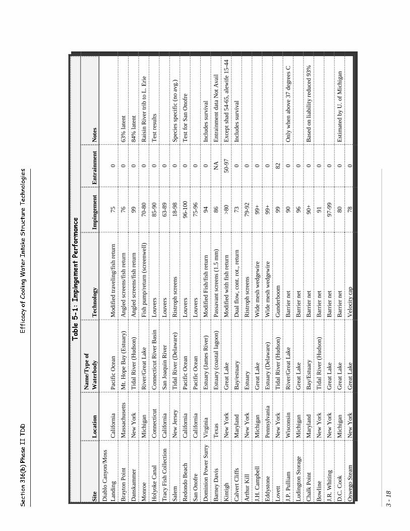
Sect
ion
316
(b)
Phas
e I
I T
DD
Eff
icac
y of
Coo
ling
Wat
er
Int
ake S
truc
ture
Tech
nolo
gies
3 -
18
Table 5
-1:
Impingement
Perf
orm
ance
Site
Loc
atio
nN
ame/
Typ
e of
Wat
erbo
dyT
echn
olog
yIm
ping
emen
tE
ntra
inm
ent
Not
es
Dia
blo
Can
yon/
Mos
sL
andi
ngC
alif
orni
aPa
cifi
c O
cean
M
odif
ied
trav
elin
g/fi
sh r
etur
n75
0
Bra
yton
Poi
ntM
assa
chus
etts
Mt.
Hop
e B
ay (
Est
uary
)A
ngle
d sc
reen
s/fi
sh r
etur
n76
063
% la
tent
Dan
skam
mer
N
ew Y
ork
Tid
al R
iver
(H
udso
n)A
ngle
d sc
reen
s/fi
sh r
etur
n99
084
% la
tent
Mon
roe
Mic
higa
nR
iver
/Gre
at L
ake
Fish
pum
p/re
turn
(sc
reen
wel
l)70
-80
0R
aisi
n R
iver
trib
to L
. Eri
e
Hol
yoke
Can
alC
onne
ctic
utC
onne
ctic
ut R
iver
Bas
inL
ouve
rs85
-90
0T
est r
esul
ts
Tra
cy F
ish
Col
lect
ion
Cal
ifor
nia
San
Joaq
uin
Riv
erL
ouve
rs63
-89
0
Sale
mN
ew J
erse
yT
idal
Riv
er (
Del
awar
e)R
istr
oph
scre
ens
18-9
80
Spec
ies
spec
ific
(no
avg
.)
Red
ondo
Bea
chC
alif
orni
aPa
cifi
c O
cean
Lou
vers
96-1
000
Tes
t for
San
Ono
fre
San
Ono
fre
Cal
ifor
nia
Paci
fic
Oce
anL
ouve
rs75
-96
0
Dom
inio
n Po
wer
Sur
ryV
irgi
nia
Est
uary
(Ja
mes
Riv
er)
Mod
ifie
d Fi
sh/f
ish
retu
rn94
0In
clud
es s
urvi
val
Bar
ney
Dav
is
Tex
asE
stua
ry (
coas
tal l
agoo
n)Pa
ssav
ant s
cree
ns (
1.5
mm
)86
NA
Ent
rain
men
t dat
a N
ot A
vail
Kin
tigh
New
Yor
kG
reat
Lak
e M
odif
ied
wit
h fi
sh r
etur
n>8
050
-97
Exc
ept s
had
54-6
5, a
lew
ife
15-4
4
Cal
vert
Cli
ffs
Mar
ylan
dB
ay/e
stua
ryD
ual f
low
, con
t. ro
t., r
etur
n73
0In
clud
es s
urvi
val
Art
hur
Kil
lN
ew Y
ork
Est
uary
Ris
trop
h sc
reen
s79
-92
0
J.H
. Cam
pbel
lM
ichi
gan
Gre
at L
ake
Wid
e m
esh
wed
gew
ire
99+
0
Edd
ysto
nePe
nnsy
lvan
iaE
stua
ry (
Del
awar
e)W
ide
mes
h w
edge
wir
e 99
+0
Lov
ett
New
Yor
kT
idal
Riv
er (
Hud
son)
Gun
derb
oom
9982
J.P.
Pul
liam
Wis
cons
inR
iver
/Gre
at L
ake
Bar
rier
net
90
0O
nly
whe
n ab
ove
37 d
egre
es C
Lud
ingt
on S
tora
geM
ichi
gan
Gre
at L
ake
Bar
rier
net
96
0
Cha
lk P
oint
Mar
ylan
dB
ay/E
stua
ryB
arri
er n
et
90+
0B
ased
on
liab
ilit
y re
duce
d 93
%
Bow
line
New
Yor
kT
idal
Riv
er (
Hud
son)
Bar
rier
net
91
0
J.R
. Whi
ting
New
Yor
kG
reat
Lak
e B
arri
er n
et
97-9
90
D.C
. Coo
kM
ichi
gan
Gre
at L
ake
Bar
rier
net
80
0E
stim
ated
by
U. o
f M
ichi
gan
Osw
ego
Stea
mN
ew Y
ork
Gre
at L
ake
Vel
ocit
y ca
p78
0
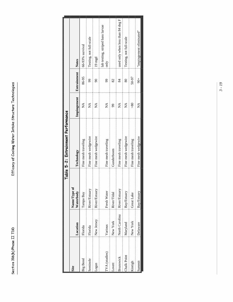
Sect
ion
316
(b)
Phas
e I
I T
DD
Eff
icac
y of
Coo
ling
Wat
er
Int
ake S
truc
ture
Tech
nolo
gies
3 -
19
Table 5
-2:
Entr
ainment
Perf
orm
ance
Site
Loc
atio
nN
ame/
Typ
e of
Wat
erbo
dyT
echn
olog
yIm
ping
emen
tE
ntra
inm
ent
Not
es
Big
Ben
dFl
orid
aT
ampa
Bay
Fine
mes
h tr
avel
ing
NA
86-9
566
-93%
sur
viva
l
Sem
inol
eFl
orid
aR
iver
/Est
uary
Fine
mes
h w
edge
wir
eN
A99
Tes
ting
, not
ful
l-sc
ale
Log
anN
ew J
erse
yR
iver
/Est
uary
Fine
mes
h w
edge
wir
eN
A90
19 m
gd
TV
A (
stud
ies)
Var
ious
Fres
h W
ater
Fine
mes
h tr
avel
ing
NA
99la
b te
stin
g, s
trip
ed b
ass
larv
aeon
ly
Lov
ett
New
Yor
kR
iver
/Tid
alG
unde
rboo
m99
82
Bru
nsw
ick
Nor
th C
arol
ina
Riv
er/E
stua
ryFi
ne m
esh
trav
elin
gN
A84
used
onl
y w
hen
less
than
84
deg
F
Cha
lk P
oint
Mar
ylan
dB
ay/E
stua
ryFi
ne m
esh
wed
gew
ire
NA
80T
esti
ng, n
ot f
ull-
scal
e
Kin
tigh
New
Yor
kG
reat
Lak
eFi
ne m
esh
trav
elin
g>8
050
-97
Sum
mit
Del
awar
eB
ay/E
stua
ryFi
ne m
esh
wed
gew
ire
NA
90+
"im
ping
emen
t eli
min
ated
"

Section 316(b) Phase II TDD Efficacy of Cooling Water Intake Structure Technologies
3 - 20
REFERENCES
American Electric Power Corporation. March, 1980. Philip Sporn Plant 316(b) Demonstration Document.
American Society of Civil Engineers. 1982. Design of Water Intake Structures for FishProtection. Task Committee on Fish-Handling Capability of Intake Structures of theCommittee on Hydraulic Structures of the Hydraulic Division of the American Society ofCivil Engineers.
Bailey et. al. Undated. Studies of Cooling Water Intake Structure Effects at PEPCO Generating Stations.
CK Environmental. June, 2000. Letter from Charles Kaplan, CK Environmental, to Martha Segall, Tetra Tech,Inc. June 26, 2000.
Duke Energy, Inc. April, 2000. Moss Landing Power Plant Modernization Project, 316(b) Resource Assessment.
Ecological Analysts, Inc. 1979. Evaluation of the Effectiveness of a Continuously Operating Fine Mesh TravelingScreen for Reducing Ichthyoplankton Entrainment at the Indian Point Generating Station. Prepared forConsolidated Edison, Inc.
Edison Electric Institute (EEI). 1993. EEI Power Statistics Database. Prepared by theUtility Data Institute for the Edison Electric Institute.
Ehrler, C. and Raifsnider, C. April, 1999. “Evaluation of the Effectiveness of Intake Wedgewire Screens.” Presented at EPRI Power Generation Impacts on Aquatic Resources Conference.
Electric Power Research Institute (EPRI). 1999. Fish Protection at Cooling Water Intakes: Status Report.
EPRI. March, 1989. Intake Technologies: Research Status. Publication GS-6293.
EPRI. 1985. Intake Research Facilities Manual.
ESSA Technologies, Ltd. June, 2000. Review of Portions of NJPDES Renewal Application for the PSE&GSalem Generating Station.
Fletcher, I. 1990. Flow Dynamics and Fish Recovery Experiments: Water Intake Systems.
Florida Power and Light. August, 1995. Assessment of the Impacts of the St. Lucie Nuclear Generating Plant onSea Turtle Species Found in the Inshore Waters of Florida.
Fritz, E.S. 1980. Cooling Water Intake Screening Devices Used to Reduce Entrainmentand Impingement. Topical Briefs: Fish and Wildlife Resources and Electric PowerGeneration, No. 9.
Hadderingh, R.H. 1979. “Fish Intake Mortality at Power Stations, the Problem and itsRemedy.” In: Hydrological Bulletin, 13(2-3).
Hutchison, J.B., and Matousek, J.A. Undated. Evaluation of a Barrier Net Used to Mitigate Fish Impingement at aHudson River Power Pant Intake. American Fisheries Society Monograph.
Jude, D.J. 1976. “Entrainment of Fish Larvae and Eggs on the Great Lakes, with Special Reference to the D.C.

Section 316(b) Phase II TDD Efficacy of Cooling Water Intake Structure Technologies
3 - 21
Cook Nuclear Plant, Southeastern Lake Michigan.” In: Jensen, L.D. (Ed.), Third National Workshop onEntrainment & Impingement: Section 316(b) – Research and Compliance.
Ketschke, B.A. 1981. “Field and Laboratory Evaluation of the Screening Ability of a Porous Dike.” In: P.B.Dorn and Johnson (Eds.). Advanced Intake Technology for Power Plant Cooling Water Systems.
King, R.G. 1977. “Entrainment of Missouri River Fish Larvae through Fort Calhoun Station.” In: Jensen, L.D.(Ed.), Fourth National Workshop on Entrainment and Impingement.
Lifton, W.S. Undated. Biological Aspects of Screen Testing on the St. John’s River, Palatka, Florida.
Marley Cooling Tower. August 2001. Electronic Mail from Robert Fleming, Marley Cooling Tower to RonRimelman, Tetra Tech, Inc. August 9, 2001.
Micheletti, W. September, 1987. “Fish Protection at Cooling Water Intake Systems.” In: EPRI Journal.
Mussalli, Y.G., Taft, E.P., and Hofmann, P. February, 1978. “Biological and Engineering Considerations in theFine Screening of Small Organisms from Cooling Water Intakes.” In: Proceedings of the Workshop on LarvalExclusion Systems for Power Plant Cooling Water Intakes, Sponsored by Argonne National Laboratory (ANLPublication No. ANL/ES-66).
Mussalli, Y.G., Taft, E.P, and Larsen, J. November, 1980. "Offshore Water IntakesDesignated to Protect Fish." In: Journal of the Hydraulics Division, Proceedings of theAmerica Society of Civil Engineers. Vol. 106, No HY11.
Northeast Utilities Service Company. January, 1993. Feasibility Study of Cooling Water System Alternatives toReduce Winter Flounder Entrainment at Millstone Units 1-3.
Orange and Rockland Utilities and Southern Energy Corp. 2000. Lovett Generating Station GunderboomEvaluation Program, 1999.
PG&E. March 2000. Diablo Canyon Power Plant, 316(b) Demonstration Report.
Pagano, R. and Smith, W.H.B. November, 1977. Recent Developments in Techniques toProtect Aquatic Organisms at the Intakes Steam-Electric Power Plants.
Pisces Conservation, Ltd. 2001. Technical Evaluation of USEPA’s Proposed Cooling Water Intake Regulations forNew Facilities, November 2000.
Richards, R.T. December, 1977. "Present Engineering Limitations to the Protection of Fishat Water Intakes". In: Fourth National Workshop on Entrainment and Impingement.
Ringger, T.J. April, 1999. “Baltimore Gas and Electric, Investigations of Impingement of Aquatic Organisms atthe Calvert Cliffs Nuclear Power Plant, 1975-1999.” Presented at EPRI Power Generation Impacts on AquaticResources Conference.
Sharma, R.K. February, 1978. "A Synthesis of Views Presented at the Workshop." In: Larval Exclusion Systems For Power Plant Cooling Water Intakes.
Taft, E.P. April, 1999. “Alden Research Laboratory, Fish Protection Technologies: A Status Report.” Presentedat EPRI Power Generation Impacts on Aquatic Resources Conference.

Section 316(b) Phase II TDD Efficacy of Cooling Water Intake Structure Technologies
3 - 22
Taft, E.P. March, 1999. PSE&G Renewal Application, Appendix F, Salem Generation Station.
Taft, E.P. et. al. 1981. “Laboratory Evaluation of the Larval Fish Impingement and Diversion Systems.” In: Proceedings of Advanced Intake Technology.
Tennessee Valley Authority (TVA). 1976. A State of the Art Report on Intake Technologies.
U.S. Environmental Protection Agency (EPA), Region 4. May, 1983. 316a and 316b Finding for CapeCanaveral/Orlando Utilities Plants at Canaveral Pool.
EPA, Region 4. September, 1979. Brunswick Nuclear Steam Electric Generating Plant. Historical Summary andReview of Section 316(b) Issues.
University of Michigan. 1985. Impingement Losses at the D.C. Cook Nuclear Power Plant During 1975-1982with a Discussion of Factors Responsible and Possible Impact on Local Populations.
Versar, Inc. April, 1990. Evaluation of the Section 316 Status of Delaware Facilities with Cooling WaterDischarges. Prepared for State of Delaware Department of Natural Resources.
Weisberg, S.B., Jacobs, F., Burton, W.H., and Ross, R.N. 1983. Report on PreliminaryStudies Using the Wedge Wire Screen Model Intake Facility. Prepared for State ofMaryland, Power Plant Siting Program.

Section 316(b) Phase II TDD Efficacy of Cooling Water Intake Structure Technologies
3 - 23

§ 316(b) Phase II TDD Attachment A to Chapter 3
Attachment A to Chapter 3
COOLING WATER INTAKE STRUCTURE TECHNOLOGY FACT SHEETS

§ 316(b) Phase II TDD Attachment A to Chapter 3
A-2
Intake Screening Systems Fact Sheet No. 1: Single-Entry, Single-ExitVertical Traveling Screens (ConventionalTraveling Screens)
Description:
The single-entry, single-exit vertical traveling screens (conventional traveling screens) consistof screen panels mounted on an endless belt; the belt rotates through the water vertically. Thescreen mechanism consists of the screen, the drive mechanism, and the spray cleaning system.Most of the conventional traveling screens are fitted with 3/8-inch mesh and are designed toscreen out and prevent debris from clogging the pump and the condenser tubes. The screen meshis usually supplied in individual removable panels referred to as “ baskets” or “trays”.
The screen washing system consists of a line of spray nozzles operating at a relatively highpressure of 80 to 120 pounds per square inch (psi). The screens are usually designed to rotateat a single speed. The screens are rotated either at predetermined intervals or when apredetermined differential pressure is reached across the screens based on the amount of debrisin the intake waters.
Because of this intermittent operation of the conventional traveling screens, fish can becomeimpinged against the screens during the extended period of time while the screens are stationaryand eventually die. When the screens are rotated the fish are removed from the water and thensubjected to a high pressure spray; the fish may fall back into the water and become re-impinged or they may be damaged (EPA, 1976, Pagano et al, 1977).
Testing Facilities and/or Facilities Using the Technology:
C The conventional traveling screens are the most common screening device presentlyused at steam electric power plants. Sixty percent of all the facilities use thistechnology at their intake structure (EEI, 1993).
Research/Operation Findings:
C The conventional single-entry single screen is the most common device resulting inimpacts from entrainment and impingement (Fritz, 1980).
Design Considerations:
C The screens are usually designed structurally to withstand a differential pressure acrosstheir face of 4 to 8 feet of water.
C The recommended normal maximum water velocity through the screen is about 2.5 feetper second (ft/sec). This recommended velocity is where fish protection is not a factorto consider.
C The screens normally travel at one speed (10 to 12 feet per minute) or two speeds (2.5
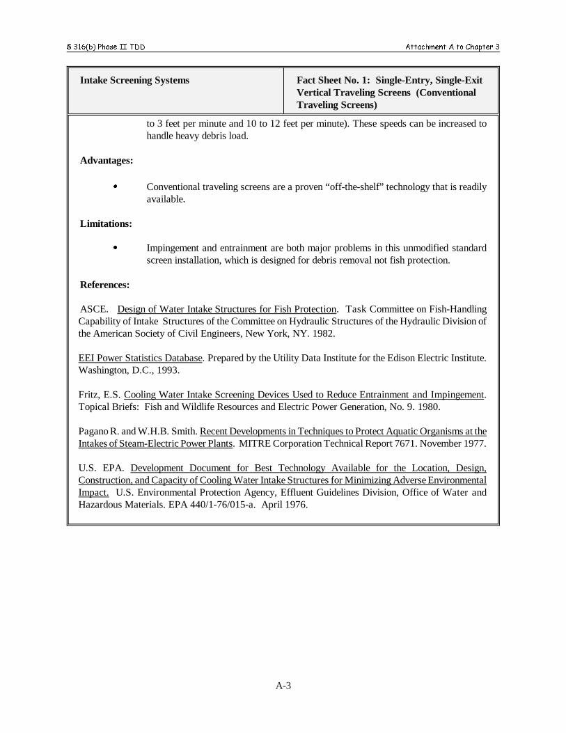
§ 316(b) Phase II TDD Attachment A to Chapter 3
Intake Screening Systems Fact Sheet No. 1: Single-Entry, Single-ExitVertical Traveling Screens (ConventionalTraveling Screens)
A-3
to 3 feet per minute and 10 to 12 feet per minute). These speeds can be increased tohandle heavy debris load.
Advantages:
C Conventional traveling screens are a proven “off-the-shelf” technology that is readilyavailable.
Limitations:
C Impingement and entrainment are both major problems in this unmodified standardscreen installation, which is designed for debris removal not fish protection.
References:
ASCE. Design of Water Intake Structures for Fish Protection. Task Committee on Fish-HandlingCapability of Intake Structures of the Committee on Hydraulic Structures of the Hydraulic Division ofthe American Society of Civil Engineers, New York, NY. 1982.
EEI Power Statistics Database. Prepared by the Utility Data Institute for the Edison Electric Institute.Washington, D.C., 1993.
Fritz, E.S. Cooling Water Intake Screening Devices Used to Reduce Entrainment and Impingement.Topical Briefs: Fish and Wildlife Resources and Electric Power Generation, No. 9. 1980.
Pagano R. and W.H.B. Smith. Recent Developments in Techniques to Protect Aquatic Organisms at theIntakes of Steam-Electric Power Plants. MITRE Corporation Technical Report 7671. November 1977.
U.S. EPA. Development Document for Best Technology Available for the Location, Design,Construction, and Capacity of Cooling Water Intake Structures for Minimizing Adverse EnvironmentalImpact. U.S. Environmental Protection Agency, Effluent Guidelines Division, Office of Water andHazardous Materials. EPA 440/1-76/015-a. April 1976.
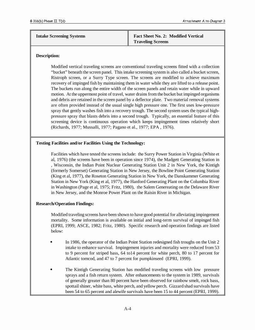
§ 316(b) Phase II TDD Attachment A to Chapter 3
A-4
Intake Screening Systems Fact Sheet No. 2: Modified VerticalTraveling Screens
Description:
Modified vertical traveling screens are conventional traveling screens fitted with a collection“bucket” beneath the screen panel. This intake screening system is also called a bucket screen,Ristroph screen, or a Surry Type screen. The screens are modified to achieve maximumrecovery of impinged fish by maintaining them in water while they are lifted to a release point.The buckets run along the entire width of the screen panels and retain water while in upwardmotion. At the uppermost point of travel, water drains from the bucket but impinged organismsand debris are retained in the screen panel by a deflector plate. Two material removal systemsare often provided instead of the usual single high pressure one. The first uses low-pressurespray that gently washes fish into a recovery trough. The second system uses the typical high-pressure spray that blasts debris into a second trough. Typically, an essential feature of thisscreening device is continuous operation which keeps impingement times relatively short(Richards, 1977; Mussalli, 1977; Pagano et al., 1977; EPA , 1976).
Testing Facilities and/or Facilities Using the Technology:
Facilities which have tested the screens include: the Surry Power Station in Virginia (White etal, 1976) (the screens have been in operation since 1974), the Madgett Generating Station in, Wisconsin, the Indian Point Nuclear Generating Station Unit 2 in New York, the Kintigh(formerly Somerset) Generating Station in New Jersey, the Bowline Point Generating Station(King et al, 1977), the Roseton Generating Station in New York, the Danskammer GeneratingStation in New York (King et al, 1977), the Hanford Generating Plant on the Columbia Riverin Washington (Page et al, 1975; Fritz, 1980), the Salem Genereating on the Delaware Riverin New Jersey, and the Monroe Power Plant on the Raisin River in Michigan.
Research/Operation Findings:
Modified traveling screens have been shown to have good potential for alleviating impingementmortality. Some information is available on initial and long-term survival of impinged fish(EPRI, 1999; ASCE, 1982; Fritz, 1980). Specific research and operation findings are listedbelow:
C In 1986, the operator of the Indian Point Station redesigned fish troughs on the Unit 2intake to enhance survival. Impingement injuries and mortality were reduced from 53to 9 percent for striped bass, 64 to14 percent for white perch, 80 to 17 percent forAtlantic tomcod, and 47 to 7 percent for pumpkinseed (EPRI, 1999).
C The Kintigh Generating Station has modified traveling screens with low pressuresprays and a fish return system. After enhancements to the system in 1989, survivalsof generally greater than 80 percent have been observed for rainbow smelt, rock bass,spottail shiner, white bass, white perch, and yellow perch. Gizzard shad survivals havebeen 54 to 65 percent and alewife survivals have been 15 to 44 percent (EPRI, 1999).
§ 316(b) Phase II TDD Attachment A to Chapter 3
Intake Screening Systems Fact Sheet No. 2: Modified VerticalTraveling Screens
A-5
C Long-term survival testing was conducted at the Hanford Generating Plant on theColumbia River (Page et al, 1975; Fritz, 1980). In this study, 79 to 95 percent of theimpinged and collected Chinook salmon fry survived for over 96 hours.
C Impingement data collected during the 1970s from Dominion Power’s Surry Stationindicated a 93.8 percent survival rate of all fish impinged. Bay anchovies had the lowestsurvival rate of 83 percent. The facility has modified Ristroph screens with lowpressure wash and fish return systems (EPRI 1999).
C At the Arthur Kill Station, 2 of 8 screens are modified Ristroph type; the remaining sixscreens are conventional type. The modified screens have fish collection troughs, lowpressure spray washes, fish flap seals, and separate fish collection sluices. 24-hoursurvival for the unmodified screens averages 15 percent, while the two modified screenshave 79 and 92 percent average survival rates (EPRI 1999).
Design Considerations:
C The same design considerations as for Fact Sheet No. 1: Conventional VerticalTraveling Screens apply (ASCE, 1982).
Advantages:
C Traveling screens are a proven “off-the-shelf” technology that is readily available. Anessential feature of such screens is continuous operation during periods where fish arebeing impinged compared to conventional traveling screens which operate on anintermittent basis
Limitations:
C The continuous operation can result in undesirable maintenance problems (Mussalli,1977).
C Velocity distribution across the face of the screen is generally very poor.
Latent mortality can be high, especially where fragile species are present.
References:
ASCE. Design of Water Intake Structures for Fish Protection. Task Committee on Fish-HandlingCapability of Intake Structures of the Committee on Hydraulic Structures of the HydraulicDivision of the American Society of Civil Engineers, New York, NY. 1982.
Electric Power Research Institute (EPRI). Fish Protection at Cooling Water Intakes: Status Report.1999.
§ 316(b) Phase II TDD Attachment A to Chapter 3
Intake Screening Systems Fact Sheet No. 2: Modified VerticalTraveling Screens
A-6
EPRI. Intake Technologies: Research Status. Electric Power Research Institute GS-6293. March 1989.
U.S. EPA. Development Document for Best Technology Available for the Location, design,Construction, and Capacity of Cooling Water Intake Structures for Minimizing AdverseEnvironmental Impact. Environmental Protection Agency, Effluent Guidelines Division, Officeof Water and Hazardous Materials, EPA 440/1-76/015-a. April 1976.
Fritz, E.S. Cooling Water Intake Screening Devices Used to Reduce Entrainment and Impingement.Topical Briefs: Fish and Wildlife Resources and Electric Power Generation, No. 9, 1980.
King, L.R., J.B. Hutchinson, Jr. and T.G. Huggins. “Impingement Survival Studies on White Perch,Striped Bass, and Atlantic Tomcod at Three Hudson Power Plants”. In Fourth NationalWorkshop on Entrainment and Impingement, L.D. Jensen (Editor) Ecological Analysts, Inc.,Melville, NY. Chicago, December 1977.
Mussalli, Y.G., “Engineering Implications of New Fish Screening Concepts”. In Fourth NationalWorkshop on Entrainment and Impingement, L.D. Jensen (Editor). Ecological Analysts, Inc.,Melville, N.Y. Chicago, December 1977, pp 367-376.
Pagano, R. and W.H.B. Smith. Recent Developments in Techniques to Protect Aquatic Organisms atthe Intakes Steam-Electric Power Plants. MITRE Technical Report 7671. November 1977.
Richards, R.T. “Present Engineering Limitations to the Protection of Fish at Water Intakes”. In FourthNational Workshop on Entrainment and Impingement, pp 415-424. L.D. Jensen (Editor).Ecological Analysts, Inc., Melville, N.Y. Chicago, December 1977.
White, J.C. and M.L. Brehmer. “Eighteen-Month Evaluation of the Ristroph Traveling Fish Screens”.In Third National Workshop on Entrainment and Impingement. L.D. Jensen (Editor). EcologicalAnalysts, Inc., Melville, N.Y. 1976.
§ 316(b) Phase II TDD Attachment A to Chapter 3
A-7
Intake Screening Systems Sheet No. 3: Inclined Single-Entry, Single-Exit Traveling Screens (AngledScreens)
Description:
Inclined traveling screens utilize standard through-flow traveling screens where the screens areset at an angle to the incoming flow as shown in the figure below. Angling the screens improvesthe fish protection effectiveness of the flush mounted vertical screens since the fish tend to avoidthe screen face and move toward the end of the screen line, assisted by a component of theinflow velocity. A fish bypass facility with independently induced flow must be provided. Thefish have to be lifted by fish pump, elevator, or conveyor and discharged to a point of safetyaway from the main water intake (Richards, 1977).
Testing Facilities and/or Facilities Using the Technology:
Angled screens have been tested/used at the following facilities: the Brayton Point Station Unit4 in Massachusetts; the San Onofre Station in California; and at power plants on Lake Ontarioand the Hudson River (ASCE, 1982; EPRI, 1999).
Research/operation Findings:
C Angled traveling screens with a fish return system have been used on the intake forBrayton Point Unit 4. Studies from 1984 through 1986 that evaluated the angledscreens showed a diversion efficiency of 76 percent with latent survival of 63 percent.Much higher results were observed excluding bay anchovy. Survival efficiency for themajor taxa exhibited an extremely wide range, from 0.1 percent for bay anchovy to 97percent for tautog. Generally, the taxa fell into two groups: a hardy group withefficiency greater than 65 percent and a sensitive group with efficiency less than 25percent (EPRI, 1999).
C Southern California Edison at its San Onofre steam power plant had more success withangled louvers than with angled screens. The angled screen was rejected for full-scaleuse because of the large bypass flow required to yield good guidance efficiencies in thetest facility.
Design Considerations:
Many variables influence the performance of angled screens. The following recommendedpreliminary design criteria were developed in the studies for the Lake Ontario and Hudson Riverintakes (ASCE, 1982):
C Angle of screen to the waterway: 25 degrees
C Average velocity of approach in the waterway upstream of the screens: 1 foot persecond
§ 316(b) Phase II TDD Attachment A to Chapter 3
Intake Screening Systems Sheet No. 3: Inclined Single-Entry, Single-Exit Traveling Screens (AngledScreens)
A-8
C Ratio of screen velocity to bypass velocity: 1:1
C Minimum width of bypass opening: 6 inches
Advantages:
C The fish are guided instead of being impinged.
C The fish remain in water and are not subject to high pressure rinsing.
Limitations:
C Higher cost than the conventional traveling screen
C Angled screens need a stable water elevation.
C Angled screens require fish handling devices with independently induced flow(Richards, 1977).
References:
ASCE. Design of Water Intake Structures for Fish Protection. Task Committee on Fish-HandlingCapability of Intake Structures of the Committee on Hydraulic Structures of the Hydraulic Divisionof the American Society of Civil Engineers, New York, NY. 1982.
Electric Power Research Institute (EPRI). Fish Protection at Cooling Water Intakes: Status Report.1999.
U.S. EPA. Development Document for Best Technology Available for the Location, Design,Construction, and Capacity of Cooling Water Intake Structures for Minimizing Adverse EnvironmentalImpact. U.S. Environmental Protection Agency, Effluent Guidelines Division, Office of Water andHazardous Materials. EPA 440/1-76/015-a. April 1976.
Richards, R.T. “Present Engineering Limitations to the Protection of Fish at Water Intakes”. In FourthNational Workshop on Entrainment and Impingement, L.D. Jensen (Editor). Ecological Analysts, Inc.,Melville, N.Y. Chicago. December 1977. pp 415-424.
§ 316(b) Phase II TDD Attachment A to Chapter 3
A-9
Intake Screening Systems Fact Sheet No.4: Fine Mesh ScreensMounted on Traveling Screens
Description:
Fine mesh screens are used for screening eggs, larvae, and juvenile fish from cooling waterintake systems. The concept of using fine mesh screens for exclusion of larvae relies on gentleimpingement on the screen surface or retention of larvae within the screening basket, washingof screen panels or baskets to transfer organisms into a sluiceway, and then sluicing theorganisms back to the source waterbody (Sharma, 1978). Fine mesh with openings as smallas 0.5 millimeters (mm) has been used depending on the size of the organisms to be protected.Fine mesh screens have been used on conventional traveling screens and single-entry, double-exit screens. The ultimate success of an installation using fine mesh screens is contingent on theapplication of satisfactory handling and recovery facilities to allow the safe return of impingedorganisms to the aquatic environment (Pagano et al, 1977).
Testing Facilities and/or Facilities Using the Technology:
The Big Bend Power Plant along Tampa Bay area has an intake canal with 0.5-mm meshRistroph screens that are used seasonally on the intakes for Units 3 and 4. At the BrunswickPower Plant in North Carolina, fine mesh used seasonally on two of four screens has shown 84percent reduction in entrainment compared to the conventional screen systems.
Research/Operation Findings:
C During the mid-1980s when the screens were initially installed at Big Bend, theirefficiency in reducing impingement and entrainment mortality was highly variable. The operator evaluated different approach velocities and screen rotational speeds. In addition, the operator recognized that frequent maintenance (manual cleaning)was necessary to avoid biofouling. By 1988, system performance had improvedgreatly. The system’s efficiency in screening fish eggs (primarily drums and bayanchovy) exceeded 95 percent with 80 percent latent survival for drum and 93percent for bay anchovy. For larvae (primarily drums, bay anchovies, blennies, andgobies), screening efficiency was 86 percent with 65 percent latent survival fordrum and 66 percent for bay anchovy. Note that latent survival in control sampleswas also approximately 60 percent (EPRI, 1999).
C At the Brunswick Power Plant in North Carolina, fine mesh screen has led to 84percent reduction in entrainment compared to the conventional screen systems. Similar results were obtained during pilot testing of 1-mm screens at the Chalk PointGenerating Station in Maryland. At the Kintigh Generating Station in New Jersey,pilot testing indicated 1-mm screens provided 2 to 35 times reductions inentrainment over conventional 9.5-mm screens (EPRI, 1999).
C Tennessee Valley Authority (TVA) pilot-scale studies performed in the 1970sshowed reductions in striped bass larvae entrainment up to 99 percent using a 0.5-

§ 316(b) Phase II TDD Attachment A to Chapter 3
Intake Screening Systems Fact Sheet No.4: Fine Mesh ScreensMounted on Traveling Screens
A-10
mm screen and 75 and 70 percent for 0.97-mm and 1.3-mm screens. A full-scaletest by TVA at the John Sevier Plant showed less than half as many larvae entrainedwith a 0.5-mm screen than 1.0 and 2.0-mm screens combined (TVA, 1976).
C Preliminary results from a study initiated in 1987 by the Central Hudson and GasElectric Corporation indicated that the fine mesh screens collect smaller fishcompared to conventional screens; mortality for the smaller fish was relatively high,with similar survival between screens for fish in the same length category (EPRI,1989).
Design Considerations:
Biological effectiveness for the whole cycle, from impingement to survival in the sourcewater body, should be investigated thoroughly prior to implementation of this option. Thisincludes:
C The intake velocity should be low so that if there is any impingement of larvae onthe screens, it is gentle enough not to result in damage or mortality.
C The wash spray for the screen panels or the baskets should be low-pressure so as notto result in mortality.
C The sluiceway should provide smooth flow so that there are no areas of highturbulence; enough flow should be maintained so that the sluiceway is not dry at anytime.
C The species life stage, size and body shape and the ability of the organisms towithstand impingement should be considered with time and flow velocities.
C The type of screen mesh material used is important. For instance, synthetic meshesmay be smooth and have a low coefficient of friction, features that might help tominimize abrasion of small organisms. However, they also may be more susceptibleto puncture than metallic meshes (Mussalli, 1977).
Advantages:
C There are indications that fine mesh screens reduce entrainment.
Limitations:
C Fine mesh screens may increase the impingement of fish, i.e., they need to be used inconjunction with properly designed and operated fish collection and return systems.
C Due to the small screen openings, these screens will clog much faster than those withconventional 3/8-inch mesh. Frequent maintenance is required, especially in marine
§ 316(b) Phase II TDD Attachment A to Chapter 3
Intake Screening Systems Fact Sheet No.4: Fine Mesh ScreensMounted on Traveling Screens
A-11
environments.
References:
Bruggemeyer, V., D. Condrick, K. Durrel, S. Mahadevan, and D. Brizck. “Full Scale OperationalDemonstration of Fine Mesh Screens at Power Plant Intakes”. In Fish Protection at Steam andHydroelectric Power Plants. EPRI CS/EA/AP-5664-SR, March 1988, pp 251-265.
Electric Power Research Institute (EPRI). Fish Protection at Cooling Water Intakes: Status Report.1999.
EPRI. Intake Technologies: Research Status. Electrical Power Research Institute, EPRI GS-6293.March 1989.
Pagano, R., and W.H.B. Smith. Recent Developments in Techniques to Protect Aquatic Organismsat the Intakes Steam-Electric Power Plants. MITRE Corporation Technical Report 7671. November1977.
Mussalli, Y.G., E.P. Taft, and P. Hofmann. “Engineering Implications of New Fish ScreeningConcepts”. In Fourth Workshop on Larval Exclusion Systems For Power Plant Cooling WaterIntakes, San-Diego, California, February 1978, pp 367-376.
Sharma, R.K., “A Synthesis of Views Presented at the Workshop”. In Larval Exclusion SystemsFor Power Plant Cooling Water Intakes. San-Diego, California, February 1978, pp 235-237.
Tennessee Valley Authority (TVA). A State of the Art Report on Intake Technologies. 1976.

§ 316(b) Phase II TDD Attachment A to Chapter 3
A-12
Passive Intake Systems Fact Sheet No. 5: Wedgewire Screens
Description:
Wedgewire screens are designed to reduce entrainment by physical exclusion and by exploitinghydrodynamics. Physical exclusion occurs when the mesh size of the screen is smaller than theorganisms susceptible to entrainment. Hydrodynamic exclusion results from maintenance of alow through-slot velocity, which, because of the screen’s cylindrical configuration, is quicklydissipated, thereby allowing organisms to escape the flow field (Weisberd et al, 1984). Thescreens can be fine or wide mesh. The name of these screens arise from the triangular or“wedge” cross section of the wire that makes up the screen. The screen is composed ofwedgewire loops welded at the apex of their triangular cross section to supporting axial rodspresenting the base of the cross section to the incoming flow (Pagano et al, 1977). A cylindricalwedgewire screen is shown in the figure below. Wedgewire screens are also called profilescreens or Johnson screens.
Testing Facilities and/or Facilities Using the Technology:
Wide mesh wedgewire screens are used at two large power plants, Eddystone and Campbell.Smaller facilities with wedgewire screens include Logan and Cope with fine mesh and Jeffreywith wide mesh (EPRI 1999).
Research/Operation Findings:
C In-situ observations have shown that impingement is virtually eliminated whenwedgewire screens are used (Hanson, 1977; Weisberg et al, 1984).
C At Campbell Unit 3, impingement of gizzard shad, smelt, yellow perch, alewife, andshiner species is significantly lower than Units 1 and 2 that do not have wedgewirescreens (EPRI, 1999).
C The cooling water intakes for Eddystone Units 1 and 2 were retrofitted with wedgewirescreens because over 3 million fish were reportedly impinged over a 20-month period.The wedgewire screens have generally eliminated impingement at Eddystone (EPRI,1999).
C Laboratory studies (Heuer and Tomljanovitch, 1978) and prototype field studies(Lifton, 1979; Delmarva Power and Light, 1982; Weisberg et al, 1983) have shownthat fine mesh wedgewire screens reduce entrainment.
C One study (Hanson, 1977) found that entrainment of fish eggs (striped bass), rangingin diameter from 1.8 mm to 3.2 mm, could be eliminated with a cylindrical wedgewirescreen incorporating 0.5 mm slot openings. However, striped bass larvae, measuring5.2 mm to 9.2 mm were generally entrained through a 1 mm slot at a level exceeding

§ 316(b) Phase II TDD Attachment A to Chapter 3
Passive Intake Systems Fact Sheet No. 5: Wedgewire Screens
A-13
75 percent within one minute of release in the test flume.
C At the Logan Generating Station in New Jersey, monitoring shows shows 90 percentless entrainment of larvae and eggs through the 1 mm wedgewire screen thenconventional screens. In situ testing of1 and 2-mm wedgewire screens was performedin the St. John River for the Seminole Generating Station Units 1 and 2 in Florida in thelate 1970s. This testing showed virtually no impingement and 99 and 62 percentreductions in larvae entrainment for the 1-mm and 2-mm screens, respectively, overconventional screen (9.5 mm) systems (EPRI, 1999).
Design Considerations:
C To minimize clogging, the screen should be located in an ambient current of at least 1feet per second (ft/sec).
C A uniform velocity distribution along the screen face is required to minimize theentrapment of motile organisms and to minimize the need of debris backflushing.
C In northern latitudes, provisions for the prevention of frazil ice formation on the screensmust be considered.
C Allowance should be provided below the screens for silt accumulation to avoidblockage of the water flow (Mussalli et al, 1980).
Advantages:
C Wedgewire screens have been demonstrated to reduce impingement and entrainment inlaboratory and prototype field studies.
Limitations:
C The physical size of the screening device is limiting in most passive systems, thus,requiring the clustering of a number of screening units. Siltation, biofouling and frazilice also limit areas where passive screens such as wedgewire can be utilized.
C Because of these limitations, wedgewire screens may be more suitable for closed-cyclemake-up intakes than once-through systems. Closed-cycle systems require less flow andfewer screens than once-through intakes; back-up conventional screens can thereforebe used during maintenance work on the wedge-wire screens (Mussalli et al, 1980).
References:
Delmarva Ecological Laboratory. Ecological Studies of the Nanticoke River and Nearby Area. VolII. Profile Wire Studies. Report to Delmarva Power and Light Company. 1980.

§ 316(b) Phase II TDD Attachment A to Chapter 3
Passive Intake Systems Fact Sheet No. 5: Wedgewire Screens
A-14
EEI Power Statistics Database. Prepared by the Utility Data Institute for the Edison ElectricInstitute. Washington, D.C., 1993.
Electric Power Research Institute (EPRI). Fish Protection at Cooling Water Intakes: Status Report.1999.
Hanson, B.N., W.H. Bason, B.E. Beitz and K.E. Charles. “A Practical Intake Screen whichSubstantially Reduces the Entrainment and Impingement of Early Life stages of Fish”. In FourthNational Workshop on Entrainment and Impingement, L.D. Jensen (Editor). Ecological Analysts,Inc., Melville, NY. Chicago, December 1977, pp 393-407.
Heuer, J.H. and D.A. Tomljanovitch. “A Study on the Protection of Fish Larvae at Water IntakesUsing Wedge-Wire Screening”. In Larval Exclusion Systems For Power Plant Cooling WaterIntakes. R.K. Sharmer and J.B. Palmer, eds, Argonne National Lab., Argonne, IL. February 1978,pp 169-194.
Lifton, W.S. “Biological Aspects of Screen Testing on the St. Johns River, Palatka, Florida”. InPassive Screen Intake Workshop, Johnson Division UOP Inc., St. Paul, MN. 1979.
Mussalli, Y.G., E.P. Taft III, and J. Larsen. “Offshore Water Intakes Designated to Protect Fish”.Journal of the Hydraulics Division, Proceedings of the America Society of Civil Engineers. Vol. 106,No HY11, November 1980, pp 1885-1901.
Pagano R. and W.H.B. Smith. Recent Developments in Techniques to Protect Aquatic Organisms atthe Intakes Steam-Electric Power Plants. MITRE Corporation Technical Report 7671. November1977.
Weisberg, S.B., F. Jacobs, W.H. Burton, and R.N. Ross. Report on Preliminary Studies Using theWedge Wire Screen Model Intake Facility. Prepared for State of Maryland, Power Plant SitingProgram. Prepared by Martin Marietta Environmental Center, Baltimore, MD. 1983.
Weisberg, S.B., W.H. Burton, E.A., Ross, and F. Jacobs. The effects od Screen Slot Size, ScreenDiameter, and Through-Slot Velocity on Entrainment of Estuarine Ichthyoplankton Through Wedge-Wire Screens. Martin Marrietta Environmental Studies, Columbia MD. August 1984.
§ 316(b) Phase II TDD Attachment A to Chapter 3
A-15
Passive Intake Systems Fact Sheet No. 6: Perforated Pipes
Description:
Perforated pipes draw water through perforations or slots in a cylindrical section placed in thewaterway. The term “perforated” is applied to round perforations and elongated slots as shown inthe figure below. The early technology was not efficient: velocity distribution was poor, it servedspecifically to screen out detritus, and was not used for fish protection (ASCE, 1982). Inner sleeveshave been added to perforated pipes to equalize the velocities entering the outer perforations. Waterentering a single perforated pipe intake without an internal sleeve will have a wide range of entrancevelocities and the highest will be concentrated at the supply pipe end. These systems have been usedat locations requiring small amounts of water such as make-up water. However, experience at steamelectric plants is very limited (Sharma, 1978).
Testing Facilities And/or Facilities Using the Technology:
Nine steam electric units in the U.S. use perforated pipes. Each of these units uses closed-cyclecooling systems with relatively low make-up intake flow ranging from 7 to 36 MGD (EEI,1993).
Research/Operation Findings:
C Maintenance of perforated pipe systems requires control of biofouling and removal ofdebris from clogged screens.
C For withdrawal of relatively small quantities of water, up to 50,000 gpm, the perforatedpipe inlet with an internal perforated sleeve offers substantial protection for fish. Thisparticular design serves the Washington Public Power Supply System on the ColumbiaRiver (Richards, 1977).
C No information is available on the fate of the organisms impinged at the face of suchscreens.
Design Considerations:
The design of these systems is fairly well established for various water intakes (ASCE, 1982). Advantages:
The primary advantage is the absence of a confined channel in which fish might become trapped.
Limitations:
Clogging, frazil ice formation, biofouling and removal of debris limit this technology to smallflow withdrawals.

§ 316(b) Phase II TDD Attachment A to Chapter 3
Passive Intake Systems Fact Sheet No. 6: Perforated Pipes
A-16
REFERENCES:
American Society of Civil Engineers. Task Committee on Fish-handling of Intake Structures of theCommittee of Hydraulic Structures. Design of Water Intake Structures for Fish Protection. ASCE, NewYork, N.Y. 1982.
EEI Power Statistics Database. Prepared by the Utility Data Institute for the Edison Electric Institute.Washington, D.C., 1993.
Richards, R.T. 1977. “Present Engineering Limitations to the Protection of Fish at Water Intakes”. InFourth National Workshop on Entrainment and Impingement, L.D. Jensen Editor, Chicago, December1977, pp 415-424.
Sharma, R.K. “A Synthesis of Views Presented at the Workshop”. In Larval Exclusion Systems ForPower Plant Cooling Water Intakes. San-Diego, California, February 1978, pp 235-237.
§ 316(b) Phase II TDD Attachment A to Chapter 3
A-17
Passive intake Systems Fact Sheet No. 7: Porous Dikes/LeakyDams
Description:
Porous dikes, also known as leaky dams or leaky dikes, are filters resembling a breakwatersurrounding a cooling water intake. The core of the dike consists of cobble or gravel, whichpermits free passage of water. The dike acts both as a physical and a behavioral barrier toaquatic organisms and is depicted in the figure below. The filtering mechanism includes abreakwater or some other type of barrier and the filtering core (Fritz, 1980). Tests conductedto date have indicated that the technology is effective in excluding juvenile and adult fish.However, its effectiveness in screening fish eggs and larvae is not established (ASCE, 1982).
Testing Facilities and/or Facilities Using the Technology:
C Two facilities which are both testing facilities and have used the technology are: thePoint Beach Nuclear Plant in Wisconsin and the Baily Generating Station in Indiana(EPRI, 1985). The Brayton Point Generating Station in Massachusetts has also testedthe technology.
Research/Operation Findings:
C Schrader and Ketschke (1978) studied a porous dike system at the Lakeside Plant onLake Michigan and found that numerous fish penetrated large void spaces, but for mostfish accessibility was limited.
C The biological effectiveness of screening of fish larvae and the engineeringpracticability have not been established (ASCE, 1982).
C The size of the pores in the dike dictates the degree of maintenance due to biofoulingand clogging by debris.
C Ice build-up and frazil ice may create problems as evidenced at the Point BeachNuclear Plant (EPRI, 1985).
Design Considerations:
C The presence of currents past the dike is an important factor which may probablyincrease biological effectiveness.
C The size of pores in the dike determines the extent of biofouling and clogging by debris(Sharma, 1978).
C Filtering material must be of a size that permits free passage of water but still preventsentrainment and impingement.
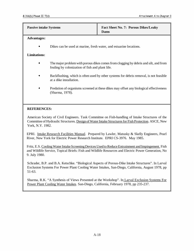
§ 316(b) Phase II TDD Attachment A to Chapter 3
Passive intake Systems Fact Sheet No. 7: Porous Dikes/LeakyDams
A-18
Advantages:
C Dikes can be used at marine, fresh water, and estuarine locations. Limitations:
C The major problem with porous dikes comes from clogging by debris and silt, and fromfouling by colonization of fish and plant life.
C Backflushing, which is often used by other systems for debris removal, is not feasibleat a dike installation.
C Predation of organisms screened at these dikes may offset any biological effectiveness(Sharma, 1978).
REFERENCES:
American Society of Civil Engineers. Task Committee on Fish-handling of Intake Structures of theCommittee of Hydraulic Structures. Design of Water Intake Structures for Fish Protection. ASCE, NewYork, N.Y. 1982.
EPRI. Intake Research Facilities Manual. Prepared by Lawler, Matusky & Skelly Engineers, PearlRiver, New York for Electric Power Research Institute. EPRI CS-3976. May 1985.
Fritz, E.S. Cooling Water Intake Screening Devices Used to Reduce Entrainment and Impingement. Fishand Wildlife Service, Topical Briefs: Fish and Wildlife Resources and Electric Power Generation, No9. July 1980.
Schrader, B.P. and B.A. Ketschke. “Biological Aspects of Porous-Dike Intake Structures”. In LarvalExclusion Systems For Power Plant Cooling Water Intakes, San-Diego, California, August 1978, pp51-63.
Sharma, R.K. “A Synthesis of Views Presented at the Workshop”. In Larval Exclusion Systems ForPower Plant Cooling Water Intakes. San-Diego, California, February 1978, pp 235-237.
§ 316(b) Phase II TDD Attachment A to Chapter 3
A-19
Fish Diversion or Avoidance Systems Fact Sheet No. 8: Louver Systems
Description:
Louver systems are comprised of a series of vertical panels placed at an angle to the direction of theflow (typically 15 to 20 degrees). Each panel is placed at an angle of 90 degrees to the direction ofthe flow (Hadderingh, 1979). The louver panels provide an abrupt change in both the flow directionand velocity (see figure below). This creates a barrier, which fish can immediately sense and willavoid. Once the change in flow/velocity is sensed by fish, they typically align with the direction ofthe current and move away laterally from the turbulence. This behavior further guides fish into acurrent created by the system, which is parallel to the face of the louvers. This current pulls the fishalong the line of the louvers until they enter a fish bypass or other fish handling device at the end ofthe louver line. The louvers may be either fixed or rotated similar to a traveling screen. Flowstraighteners are frequently placed behind the louver systems.
These types of barriers have been very successful and have been installed at numerous irrigationintakes, water diversion projects, and steam electric and hydroelectric facilities. It appears that thistechnology has, in general, become accepted as a viable option to divert juvenile and adult fish.
Testing Facilities and/or Facilities Using the Technology:
Louver barrier devices have been tested and/or are in use at the following facilities: the CaliforniaDepartment of Water Resource’s Tracy Pumping Plant; the California Department of Fish andGame’s Delta Fish Protective Facility in Bryon; the Conte Anadromous Fish Research Center inMassachusetts, and the San Onofre Nuclear Generating Station in California (EPA, 1976; EPRI,1985; EPRI, 1999). In addition, three other plants also have louvers at their facilities: the RuthFalls Power Plant in Nova Scotia, the Nine Mile Point Nuclear Power Station on Lake Erie, andT.W. Sullivan Hydroelectric Plant in Oregon. Louvers have also been tested at the Ontario HydroLaboratories in Ontario, Canada (Ray et al, 1976).
Research/Operation Findings:
Research has shown the following generalizations to be true regarding louver barriers:
1) the fish separation performance of the louver barrier decreases with an increase in the velocityof the flow through the barrier; 2) efficiency increases with fish size (EPA, 1976; Hadderingh,1979); 3) individual louver misalignment has a beneficial effect on the efficiency of the barrier; 4)the use of center walls provides the fish with a guide wall to swim along thereby improvingefficiency (EPA, 1976); and 5) the most effective slat spacing and array angle to flow depends uponthe size, species and ability of the fish to be diverted (Ray et al, 1976).
In addition, the following conclusions were drawn during specific studies:
• Testing of louvered intake structures offshore was performed at a New York facility. Thelouvers were spaced 10 inches apart to minimize clogging. The array was angled at 11.5percent to the flow. Center walls were provided for fish guidance to the bypass. Testspecies included alewife and rainbow smelt. The mean efficiency predicted was between
§ 316(b) Phase II TDD Attachment A to Chapter 3
Fish Diversion or Avoidance Systems Fact Sheet No. 8: Louver Systems
A-20
22 and 48 percent (Mussalli 1980).
• During testing at the Delta Facility’s intake in Byron California, the design flow was 6,000cubic feet per second (cfs), the approach velocity was 1.5 to 3.5 feet per second (ft/sec), andthe bypass velocities were 1.2 to 1.6 times the approach velocity. Efficiencies were foundto drop with an increase in velocity through the louvers. For example, at 1.5 to 2 ft/sec theefficiency was 61 percent for 15 millimeter long fish and 95 percent for 40 millimeter fish.At 3.5 ft/sec, the efficiencies were 35 and 70 percent (Ray et al. 1976).
• The efficiency of a louver device is highly dependent upon the length and swimmingperformance of a fish. Efficiencies of lower than 80 percent have been seen at facilitieswhere fish were less than 1 to 1.6 inches in length (Mussalli, 1980).
• In the 1990s, an experimental louver bypass system was tested at the USGS’ ConteAnadromous Fish Research Center in Massachusetts. This testing showed guidanceefficiencies for Connecticut River species of 97 percent for a “wide array” of louvers and100 percent for a “narrow array” (EPRI, 1999).
• At the Tracy Fish Collection Facility located along the San Joaquin River in California,testing was performed from 1993 and 1995 to determine the guidance efficiency of a systemwith primary and secondary louvers. The results for green and white sturgeon, Americanshad, splittail, white catfish, delta smelt, Chinook salmon, and striped bass showed meandiversion efficiencies ranging from 63 (splittail) to 89 percent (white catfish) (EPRI, 1999).
• In 1984 at the San Onofre Station, a total of 196,978 fish entered the louver system with188,583 returned to the waterbody and 8,395 impinged. In 1985, 407,755 entered thelouver system with 306,200 returned and 101,555 impinged. Therefore, the guidanceefficiencies in 1984 and 1985 were 96 and 75 percent, respectively. However, 96-hoursurvival rates for some species, i.e., anchovies and croakers, were 50 percent or less.Louvers were originally considered for use at San Onofre because of 1970s pilot testing atthe Redondo Beach Station in California where maximum guidance efficiencies of 96-100percent were observed. (EPRI, 1999)
• At the Maxwell Irrigation Canal in Oregon, louver spacing was 5.0 cm with a 98 percentefficiency of deflecting immature steelhead and above 90 percent efficiency for the samespecies with a louver spacing of 10.8 cm.
• At the Ruth Falls Power Plant in Nova Scotia, the results of a five-year evaluation forguiding salmon smelts showed that the optimum spacing was to have wide bar spacing atthe widest part of the louver with a gradual reduction in the spacing approaching thebypass. The site used a bypass:approach velocity ratio of 1.0 : 1.5 (Ray et al, 1976).
• Coastal species in California were deflected optimally (Schuler and Larson, 1974 in Rayet al, 1976) with 2.5 cm spacing of the louvers, 20 degree louver array to the direction offlow and approach velocities of 0.6 cm per second.
§ 316(b) Phase II TDD Attachment A to Chapter 3
Fish Diversion or Avoidance Systems Fact Sheet No. 8: Louver Systems
A-21
• At the T.W. Sullivan Hydroelectric Plant along the Williamette River in Oregon, the louversystem is estimated to be 92 percent effective in diverting spring Chinook, 82 percent forall Chinook, and 85 percent for steelhead. The system has been optimized to reduce fishinjuries such that the average injury occurrence is only 0.44 percent (EPRI, 1999).
Design Considerations:
The most important parameters of the design of louver barriers include the following:
• The angle of the louver vanes in relation to the channel velocity ,
• The spacing between the louvers which is related to the size of the fish,
• Ratio of bypass velocity to channel velocity,
• Shape of guide walls,
• Louver array angles, and
• Approach velocities.
Site-specific modeling may be needed to take into account species-specific considerations andoptimize the design efficiency (EPA, 1976; O’Keefe, 1978).
Advantages:
• Louver designs have been shown to be very effective in diverting fish (EPA, 1976).
Limitations:
• The costs of installing intakes with louvers may be substantially higher than othertechnologies due to design costs and the precision required during construction.
• Extensive species-specific field testing may be required.
• The shallow angles required for the efficient design of a louver system require a long lineof louvers increasing the cost as compared to other systems (Ray et al, 1976).
§ 316(b) Phase II TDD Attachment A to Chapter 3
Fish Diversion or Avoidance Systems Fact Sheet No. 8: Louver Systems
A-22
• Water level changes must be kept to a minimum to maintain the most efficient flow velocity.
• Fish handling devices are needed to take fish away from the louver barrier.
• Louver barriers may, or may not, require additional screening devices for removing solidsfrom the intake waters. If such devices are required, they may add a substantial cost to thesystem (EPA, 1976).
• Louvers may not be appropriate for offshore intakes (Mussalli, 1980).
References:
Chow, W., I.P. Murarka, R.W. Broksen. “Entrainment and Impingement in Power Plant Cooling Systems.”Literature Review. Journal Water Pollution Control Federation. 53 (6)(1981):965-973.
U.S. EPA. Development Document for Best Technology Available for the Location, Design, Construction,and Capacity of Cooling Water Intake Structures for Minimizing Adverse Environmental Impact. U.S.Environmental Protection Agency, Effluent Guidelines Division, Office of Water and Hazardous Materials.April 1976.
Electric Power Research Institute (EPRI). Fish Protection at Cooling Water Intakes: Status Report. 1999.
EPRI. Intake Research Facilities Manual. Prepared by Lawler, Matusky & Skelly Engineers, Pearl River,New York for Electric Power Research Institute. EPRI CS-3976. May 1985.
Hadderingh, R.H. “Fish Intake Mortality at Power Stations, the Problem and its Remedy.” N.V. Kema,Arnheem, Netherlands. Hydrological Bulletin 13(2-3) (1979): 83-93.
Mussalli, Y.G., E.P. Taft, and P. Hoffman. “Engineering Implications of New Fish Screening Concepts,”In Fourth National Workshop on Entrainment and impingement, L.D. Jensen (Ed.), Ecological Analysts, Inc.Melville, NY. Chicago, Dec. 1977.
Mussalli, Y.G., E.P Taft III and J. Larson. “Offshore Water Intakes Designed to Protect Fish.” Journal ofthe Hydraulics Division Proceedings of the American Society of Civil Engineers. Vol. 106 Hy11 (1980):1885-1901.
O’Keefe, W., Intake Technology Moves Ahead. Power. January 1978.
Ray, S.S. and R.L. Snipes and D.A. Tomljanovich. A State-of-the-Art Report on Intake Technologies.Prepared for Office of Energy, Minerals, and Industry, Office of Research and Development. U.S.

§ 316(b) Phase II TDD Attachment A to Chapter 3
Fish Diversion or Avoidance Systems Fact Sheet No. 8: Louver Systems
A-23
Environmental Protection Agency, Washington, D.C. by the Tennessee Valley Authority. EPA 600/7-76-020. October 1976.
Uziel, Mary S. “Entrainment and Impingement at Cooling Water Intakes.” Literature Review. JournalWater Pollution Control Federation. 52 (6) (1980): 1616-1630.
Additional References:
Adams, S.M. et al. Analysis of the Prairie Island Nuclear Generating Station- Intake Related Studies. Reportto Minnesota Pollution Control Agency. Oak Ridge National Lab. Oak Ridge TN (1979).
Bates, D.W. and R. Vinsonhaler, “The Use of Louvers for Guiding Fish.” Trans. Am. Fish. Soc. 86(1956):39-57.
Bates, D.W., and S.G., Jewett Jr., “Louver Efficiency in Deflecting Downstream Migrant Steelhead, “ Trans.Am. Fish Soc. 90(3)(1961):336-337.
Cada, G.G., and A.T. Szluha. “A Biological Evaluation of Devices Used for Reducing Entrainment andImpingement Losses at Thermal Power Plants.” In International Symposium on the Environmental Effectsof Hydraulic Engineering Works. Environmental Sciences Division, Publication No. 1276. Oak Ridge Nat’l.Lab., Oak Ridge TN (1978).
Cannon, J.B., et al. “Fish Protection at Steam Electric Power Plants: Alternative Screening Devices.” ORAL/TM-6473. Oak Ridge Nat’l. Lab. Oak Ridge, TN (1979).
Downs, D.I., and K.R. Meddock, “Design of Fish Conserving Intake System,” Journal of the PowerDivision, ASCE, Vol. 100, No. P02, Proc. Paper 1108 (1974): 191-205.
Ducharme, L.J.A. “An Application of Louver Deflectors for Guiding Atlantic Salmon (Salmo salar) Smoltsfrom Power Turbines.” Journal Fisheries Research Board of Canada 29 (1974):1397-1404.
Hallock, R.J., R.A. Iselin, and D.H.J. Fry, Efficiency Tests of the Primary Louver Systems, Tracy FishScreen, 1966-67.” Marine Resources Branch, California Department of Fish and Game (1968).
Katapodis, C. et al. A Study of Model and Prototype Culvert Baffling for Fish Passage. Fisheries andMarine Service, Tech. Report No. 828. Winnipeg, Manitoba (1978).
Kerr, J.E., “Studies on Fish Preservation at the Contra Costa Steam Plant of the Pacific Gas and ElectricCo,” California Fish and Game Bulletin No. 92 (1953).
Marcy, B.C., and M.D. Dahlberg. Review of Best Technology Available for Cooling Water Intakes. NUS
§ 316(b) Phase II TDD Attachment A to Chapter 3
Fish Diversion or Avoidance Systems Fact Sheet No. 8: Louver Systems
A-24
Corporation. Pittsburgh, PA (1978).
NUS Corp., “Review of Best Technology Available for Cooling Water Intakes.” Los Angeles Dept. of Water& Power Report, Los Angeles CA (1978).
Schuler, V.J., “Experimental Studies In Guiding Marine Fishes of Southern California with Screens andLouvers,” Ichthyol. Assoc., Bulletin 8 (1973).
Skinner, J.E. “A Functional Evaluation of Large Louver Screen Installation and Fish Facilities Research onCalifornia Water Diversion Projects.” In: L.D. Jensen, ed. Entrainment and Intake Screening. Proceedingsof the Second Entrainment and Intake Screening Workshop. The John Hopkins University, Baltimore,Maryland. February 5-9, 1973. pp 225-249 (Edison Electric Institute and Electric Power ResearchInstitute, EPRI Publication No. 74-049-00-5 (1974).
Stone and Webster Engineering Corporation, Studies to Alleviate Potential Fish Entrapment Problems -Final Report, Nine Mile Point Nuclear Station - Unit 2. Prepared for Niagara Mohawk Power Corporation,Syracuse, New York, May 1972.
Stone and Webster Engineering Corporation. Final Report, Indian Point Flume Study. Prepared forConsolidated Edison Company of New York, IN. July 1976.
Taft, E.P., and Y.G. Mussalli, “Angled Screens and Louvers for Diverting Fish at Power Plants,”Proceedings of the American Society of Civil Engineers, Journal of Hydraulics Division. Vol 104(1978):623-634.
Thompson, J.S., and Paulick, G.J. An Evaluation of Louvers and Bypass Facilities for Guiding SeawardMigrant Salmonid Past Mayfield Dam in West Washington. Washington Department of Fisheries, Olympia,Washington (1967).
Watts, F.J., “Design of Culvert Fishways.” University of Idaho Water Resources Research Institute Report,Moscow, Idaho (1974).
§ 316(b) Phase II TDD Attachment A to Chapter 3
A-25
Fish Diversion or Avoidance Systems Fact Sheet No. 9: Velocity Cap
Description:
A velocity cap is a device that is placed over vertical inlets at offshore intakes (see figurebelow). This cover converts vertical flow into horizontal flow at the entrance into the intake.The device works on the premise that fish will avoid rapid changes in horizontal flow. Fish donot exhibit this same avoidance behavior to the vertical flow that occurs without the use of sucha device. Velocity caps have been implemented at many offshore intakes and have beensuccessful in decreasing the impingement of fish.
Testing Facilities And/or Facilities Using the Technology:
The available literature (EPA, 1976; Hanson, 1979; and Pagano et al, 1977) states that velocitycaps have been installed at offshore intakes in Southern California, the Great Lakes Region, thePacific Coast, the Caribbean and overseas; however, exact locations are not specified.
Velocity caps are known to have been installed at the El Segundo, Redondo Beach, andHuntington Beach Steam Electric Stations and the San Onofre Nuclear Generation Station inSouthern California (Mussalli, 1980; Pagano et al, 1977; EPRI, 1985).
Model tests have been conducted by a New York State Utility (ASCE, 1982) and severalfacilities have installed velocity caps in the New York State /Great Lakes Area including theNine Mile Point Nuclear Station, the Oswego Steam Electric Station, and the KintighGenerating Station (EPRI, 1985).
Additional known facilities with velocity caps include the Edgewater Generation Station inWisconsin, the Seabrook Power Plant in New Hampshire, and the Nanticoke ThermalGenerating Station in Ontario, Canada (EPRI, 1985).
Research/Operation Findings:
• Horizontal velocities within a range of 0.5 to 1.5 feet per second (ft/sec) did notsignificantly affect the efficiency of a velocity cap tested at a New York facility;however, this design velocity may be specific to the species present at that site(ASCE, 1982).
• Preliminary decreases in fish entrapment averaging 80 to 90 percent were seen at theEl Segundo and Huntington Beach Steam Electric Plants (Mussalli, 1980).
• Performance of the velocity cap may be associated with cap design and the totalvolumes of water flowing into the cap rather than to the critical velocity threshold ofthe cap (Mussalli, 1980).
Design Considerations:
§ 316(b) Phase II TDD Attachment A to Chapter 3
Fish Diversion or Avoidance Systems Fact Sheet No. 9: Velocity Cap
A-26
• Designs with rims around the cap edge prevent water from sweeping around the edgecausing turbulence and high velocities, thereby providing more uniform horizontalflows (EPA, 1976; Mussalli, 1980).
• Site-specific testing should be conducted to determine appropriate velocities tominimize entrainment of particular species in the intake (ASCE, 1982).
• Most structures are sized to achieve a low intake velocity between 0.5 and 1.5 ft/secto lessen the chances of entrainment (ASCE, 1982).
• Design criteria developed for a model test conducted by Southern California EdisonCompany used a velocity through the cap of 0.5 to 1.5 ft/sec; the ratio of thedimension of the rim to the height of the intake areas was 1.5 to 1 (ASCE, 1982;Schuler, 1975).
Advantages:
• Efficiencies of velocity caps on West Coast offshore intakes have exceeded 90percent (ASCE, 1982).
Limitations:
• Velocity caps are difficult to inspect due to their location under water (EPA, 1976).
• In some studies, the velocity cap only minimized the entrainment of fish and did noteliminate it. Therefore, additional fish recovery devices are be needed in when usingsuch systems (ASCE, 1982; Mussalli, 1980).
• Velocity caps are ineffective in preventing passage of non-motile organisms andearly life stage fish (Mussalli, 1980).
References:
ASCE. Design of Water Intake Structures for Fish Protection. American Society of Civil Engineers,New York, NY. 1982.
EPRI. Intake Research Facilities Manual. Prepared by Lawler, Matusky & Skelly Engineers, PearlRiver, New York for Electric Power Research Institute. EPRI CS-3976. May 1985.
Hanson, C.H., et al. “Entrapment and Impingement of Fishes by Power Plant Cooling Water Intakes:An Overview.” Marine Fisheries Review. October 1977.
Mussalli, Y.G., E.P Taft III and J. Larson. “Offshore Water Intakes Designed to Protect Fish.” Journalof the Hydraulics Division Proceedings of the American Society of Civil Engineers, Vol. 106 Hy11(1980): 1885-1901.
§ 316(b) Phase II TDD Attachment A to Chapter 3
Fish Diversion or Avoidance Systems Fact Sheet No. 9: Velocity Cap
A-27
Pagano R. and W.H.B. Smith. Recent Development in Techniques to Protect Aquatic Organisms at theWater Intakes of Steam Electric Power Plants. Prepared for Electricite’ de France. MITRE TechnicalReport 7671. November 1977.
Ray, S.S. and R.L. Snipes and D.A. Tomljanovich. A State-of-the-Art Report on Intake Technologies.Prepared for Office of Energy, Minerals, and Industry, Office of Research and Development. U.S.Environmental Protection Agency, Washington, D.C. by the Tennessee Valley Authority. EPA 600/7-76-020. October 1976.
U.S. EPA. Development Document for Best Technology Available for the Location, Design,Construction, and Capacity of Cooling Water Intake Structures for Minimizing Adverse EnvironmentalImpact. U.S. Environmental Protection Agency, Effluent Guidelines Division, Office of Water andHazardous Materials. April 1976.
Additional References:
Maxwell, W.A. Fish Diversion for Electrical Generating Station Cooling Systems a State of the ArtReport. Southern Nuclear Engineering, Inc. Report SNE-123, NUS Corporation, Dunedin, FL. (1973)78p.
Weight, R.H. “Ocean Cooling Water System for 800 MW Power Station.” J. Power Div., Proc. Am.Soc. Civil Engr. 84(6)(1958):1888-1 to 1888-222.
Stone and Webster Engineering Corporation. Studies to Alleviate Fish Entrapment at Power PlantCooling Water Intakes, Final Report. Prepared for Niagara Mohawk Power Corporation and RochesterGas and Electric Corporation, November 1976.
Richards, R.T. “Power Plant Circulating Water Systems - A Case Study.” Short Course on theHydraulics of Cooling Water Systems for Thermal Power Plants. Colorado State University. June 1978.
§ 316(b) Phase II TDD Attachment A to Chapter 3
A-28
Fish Diversion or Avoidance Systems Fact Sheet No. 10: Fish Barrier Nets
Description:
Fish barrier nets are wide mesh nets, which are placed in front of the entrance to an intakestructure (see figure below). The size of the mesh needed is a function of the species that arepresent at a particular site. Fish barrier nets have been used at numerous facilities and lendthemselves to intakes where the seasonal migration of fish and other organisms require fishdiversion facilities for only specific times of the year.
Testing Facilities And/or Facilities Using the Technology:
The Bowline Point Generating Station, the J.P. Pulliam Power Plant in Wisconsin, theLudington Storage Plant in Michigan, and the Nanticoke Thermal Generating Station in Ontariouse barrier nets (EPRI, 1999).
Barrier Nets have been tested at the Detroit Edison Monroe Plant on Lake Erie and the ChalkPoint Station on the Patuxent River in Maryland (ASCE, 1982; EPRI, 1985). The Chalk PointStation now uses barrier nets seasonally to reduce fish and Blue Crab entry into the intake canal(EPRI, 1985). The Pickering Generation Station in Ontario evaluated rope nets in 1981illuminated by strobe lights (EPRI, 1985).
Research/Operation Findings:
• At the Bowline Point Generating Station in New York, good results (91 percentimpingement reductions) have been realized with a net placed in a V arrangementaround the intake structure (ASCE, 1982; EPRI, 1999).
• In 1980, a barrier net was installed at the J.R. Whiting Plant (Michigan) to protectMaumee Bay. Prior to net installation, 17,378,518 fish were impinged on conventionaltraveling screens. With the net, sampling in 1983 and 84 showed 421,978 fishimpinged (97 percent effective), sampling in 1987 showed 82,872 fish impinged (99percent effective), and sampling in 1991 showed 316,575 fish impinged (98 percenteffective) (EPRI, 1999).
• Nets tested with high intake velocities (greater than 1.3 feet per second) at the MonroePlant have clogged and subsequentially collapsed. This has not occurred at facilitieswhere the velocities are 0.4 to 0.5 feet per second (ASCE, 1982).
• Barrier nets at the Nanticoke Thermal Generating Station in Ontario reduced intake offish by 50 percent (EPRI, 1985).
• The J.P Pulliam Generating Station in Wisconsin uses dual barrier nets (0.64centimeters stretch mesh) to permit net rotation for cleaning. Nets are used from Aprilto December or when water temperatures go above 4 degrees Celsius. Impingement hasbeen reduced by as much as 90 percent. Operating costs run about $5,000 per year,and nets are replaced every two years at $2,500 per net (EPRI, 1985).
§ 316(b) Phase II TDD Attachment A to Chapter 3
Fish Diversion or Avoidance Systems Fact Sheet No. 10: Fish Barrier Nets
A-29
• The Chalk Point Station in Maryland realized operational costs of $5,000-10,000 peryear with the nets being replaced every two years (EPRI, 1985). However, crabimpingement has been reduced by 84 percent and overall impingrment liability has beenreduced from $2 million to $140,000 (EPRI, 1999).
• The Ludington Storage Plant (Michigan) provides water from Lake Michigan to anumber of power plant facilities. The plant has a 2.5-mile long barrier net that hassuccessfully reduced impingement and entrainment. The overall net effectiveness fortarget species (five salmonids, yellow perch, rainbow smelt, alewife, and chub) has beenover 80 percent since 1991 and 96 percent since 1995. The net is deployed from mid-April to mid-October, with storms and icing preventing use during the remainder of theyear (EPRI, 1999).
Design Considerations:
• The most important factors to consider in the design of a net barrier are the site-specificvelocities and the potential for clogging with debris (ASCE, 1982).
• The size of the mesh must permit effective operations, without excessive clogging.Designs at the Bowline Point Station in New York have 0.15 and 0.2 inch openings inthe mesh nets, while the J.P. Pulliam Plant in Wisconsin has 0.25 inch openings(ASCE, 1982).
Advantages:
• Net barriers, if operating properly, should require very little maintenance.
• Net barriers have relatively little cost associated with them.
Limitations:
• Net barriers are not effective for the protection of the early life stages of fish orzooplankton (ASCE, 1982).
References:
ASCE. Design of Water Intake Structures for Fish Protection. American Society of Civil Engineers(1982).
Electric Power Research Institute (EPRI). Fish Protection at Cooling Water Intakes: Status Report.1999.
EPRI. Intake Research Facilities Manual. Prepared by Lawler, Matusky & Skelly Engineers, PearlRiver, New York for Electric Power Research Institute. EPRI CS-3976. May 1985.

§ 316(b) Phase II TDD Attachment A to Chapter 3
Fish Diversion or Avoidance Systems Fact Sheet No. 10: Fish Barrier Nets
A-30
Lawler, Matusky, and Skelly Engineers. 1977 Hudson River Aquatic Ecology Studies at the BowlinePoint Generating Stations. Prepared for Orange and Rockland Utilities, Inc. Pearl River, NY. 1978.
§ 316(b) Phase II TDD Attachment A to Chapter 3
A-31
Fish Diversion or Avoidance Systems Fact Sheet No. 11: Aquatic Filter BarrierSystems
Description:
Aquatic filter barrier systems are barriers that employ a filter fabric designed to allow for passageof water into a cooling water intake structure, but exclude aquatic organisms. These systems aredesigned to be placed some distance from the cooling water intake structure within the sourcewaterbody and act as a filter for the water that enters into the cooling water system. Thesesystems may be floating, flexible, or fixed. Since these systems generally have such a largesurface area, the velocities that are maintained at the face of the permeable curtain are very low.One company, Gunderboom, Inc., has a patented full-water-depth filter curtain comprised ofpolyethylene or polypropylene fabric that is suspended by flotation billets at the surface of thewater and anchored to the substrate below. The curtain fabric is manufactured as a matting ofminute unwoven fibers with an apparent opening size of 20 microns. The GunderboomMarine/Aquatic Life Exclusion System (MLES)™ also employs an automated “air burst”™technology to periodically shake the material and pass air bubbles through the curtain system toclean it of sediment buildup and release any other material back in to the water column.
Testing Facilities and/or Facilities Using the Technology:
• Gunderboom MLES ™ have been tested and are currently installed on a seasonalbasis at Unit 3 of the Lovett Station in New York. Prototype testing of theGunderboom system began in 1994 as a means of lowering ichthyoplanktonentrainment at Unit 3. This was the first use of the technology at a cooling waterintake structure. The Gunderboom tested was a single layer fabric. Materialclogging resulted in loss of filtration capacity and boom submergence within 12hours of deployment. Ichthyoplankton monitoring while the boom was intactindicated an 80 percent reduction in entrainable organisms (Lawler, Matusky, andSkelly Engineers, 1996).
• A Gunderboom MLES ™ was effectively deployed at the Lovett Station for 43 daysin June and July of 1998 using an Air-Burst cleaning system and newly designeddeadweight anchoring system. The cleaning system coupled with a perforatedmaterial proved effective at limiting sediment on the boom, however it required anintensive operational schedule (Lawler, Matusky, and Skelly Engineers, 1998).
• A 1999 study was performed on the Gunderboom MLES ™ at the Lovett Station inNew York to qualitatively determine the characteristics of the fabric with respect tothe impingement of ichthyoplankton at various flow regimes. Conclusions were thatthe viability of striped bass eggs and larvae were not affected (Lawler, Matusky, andSkelly Engineers, 1999).
• Ichthyoplankton sampling at Unit 3 (with Gunderboom MLES ™ deployed) andUnit 4 (without Gunderboom) in May through August 2000 showed an overalleffectiveness of approximately 80 percent. For juvenile fish, the density at Unit 3was 58 percent lower. For post yolk-sac larvae, densities were 76 percent lower.
§ 316(b) Phase II TDD Attachment A to Chapter 3
Fish Diversion or Avoidance Systems Fact Sheet No. 11: Aquatic Filter BarrierSystems
A-32
For yolk-sac larvae, densities were 87 percent lower (Lawler, Matusky & SkellyEngineers 2000).
Research/operation Findings:
Extensive testing of the Gunderboom MLES ™ has been performed at the Lovett Station inNew York. Anchoring, material, cleaning, and monitoring systems have all been redesignedto meet the site-specific conditions in the waterbody and to optimize the operations of theGunderboom. Although this technology has been implemented at only one cooling waterintake structure, it appears to be a promising technology to reduce impingement andentrainment impacts. It is also being evaluated for use at the Contre Costa Power Plant inCalifornia.
Design Considerations:
The most important parameters in the design of a Gunderboom ® Marine/Aquatic LifeExclusion System include the following (Gunderboom, Inc. 1999):
• Size of booms designed for 3-5 gpm per square foot of submerged fabric. Flowsgreater than 10-12 gallons per minute.
• Flow-through velocity is approximately 0.02 ft/s.
• Performance monitoring and regular maintenance.
Advantages:
• Can be used in all waterbody types.
• All larger and nearly all other organisms can swim away from the barrier because oflow velocities.
• Little damage is caused to fish eggs and larvae if they are drawn up against thefabric.
• Modulized panels may easily be replaced.
• Easily deployed for seasonal use.
• Biofouling appears to be controllable through use of the sparging system.
• Impinged organisms released back into the waterbody.
• Benefits relative to cost appear to be very promising, but remain unproven to date.
§ 316(b) Phase II TDD Attachment A to Chapter 3
Fish Diversion or Avoidance Systems Fact Sheet No. 11: Aquatic Filter BarrierSystems
A-33
• Installation can occur with no or minimal plant shutdown.
Limitations:
• Currently only a proven technology for this application at one facility.
• Extensive waterbody-specific field testing may be required.
• May not be appropriate for conditions with large fluctuations in ambient flow andheavy currents and wave action.
• High level of maintenance and monitoring required.
• Recent studies have asserted that biofouling can be significant.
• Higher flow facilities may require very large surface areas; could interfere with otherwaterbody uses.
References:
Lawler, Matusky & Skelly Engineers, “Lovett Generating Station Gunderboom Evaluation Program- 1995” Prepared for Orange and Rockland Utilities, Inc. Pearl River, New York, June 1996. Lawler, Matusky & Skelly Engineers, “Lovett Generating Station Gunderboom System EvaluationProgram - 1998” Prepared for Orange and Rockland Utilities, Inc. Pearl River, New York,December 1998.
Lawler, Matusky & Skelly Engineers, “ Lovett Gunderboom Fabric Ichthyoplankton Bench ScaleTesting” Southern Energy Lovett. New York, November 1999.
Lawler, Matusky & Skelly Engineers, “Lovett 2000 Report” Prepared for Orange and RocklandUtilities, Inc. Pearl River, New York, 2000.
§ 316(b) Phase II TDD Attachment A to Chapter 3
A-34
Fish Diversion or Avoidance Systems Fact Sheet No. 12: Sound Barriers
Description:
Sound barriers are non-contact barriers that rely on mechanical or electronic equipment thatgenerates various sound patterns to elicit avoidance responses in fish. Acoustic barriers areused to deter fish from entering industrial water intakes and power plant turbines.Historically, the most widely-used acoustical barrier is a pneumatic air gun or "popper." Thepneumatic air gun is a modified seismic device which produces high-amplitude,low-frequency sounds to exclude fish. Closely related devices include "fishdrones" and“fishpulsers" (also called "hammers”). The fishdrone produces a wider range of soundfrequencies and amplitudes than the popper. The fishpulser produces a repetitive sharphammering sound of low-frequency and high-amplitude. Both instruments have ahd limitedeffectiveness in the field (EPRI, 1995; EPRI, 1989; Hanson, et al., 1977; EPA, 1976; Taft,et al., 1988; ASCE, 1992).
Researchers have generally been unable to demonstrate or apply acoustic barriers as fishdeterrents, even though fish studies showed that fish respond to sound, because the responsevaries as a function of fish species, age, and size as well as environmental factors at specificlocations. Fish may also acclimate to the sound patterns used (EPA, 1976; Taft et al., 1988;EPRI, 1995; Ray at al., 1976; Hadderingh, 1979; Hanson et al., 1977; ASCE, 1982).
Since about 1989, the application of highly refined sound generation equipment originallydeveloped for military use (e.g., sonar in submarines) has greatly advanced acoustic barriertechnology. Ibis technology has the ability to generate a wide array of frequencies, patterns,and volumes, which are monitored and controlled by computer. Video and computermonitoring provide immediate feedback on the effectiveness of an experimental soundpattern at a given location. In a particular environment, background sounds can be accountedfor, target fish species or fish populations can quickly be characterized, and the mosteffective sound pattern can be selected (Menezes, at al., 1991; Sonalysts, Inc.).
Testing Facilities and/or Facilities with Technology in Use:
No fishpulsers and pneumatic air guns are currently in use at power plant water intakes.
Research facilities that have completed studies or have on-going testing involving fishpulsersor pneumatic air guns include the Ludington Storage Plant on Lake Michigan; Nova ScotiaPower; the Hells Gate Hydroelectric Station on the Black River; the Annapolis GeneratingStation on the Bay of Fundy; Ontario Hydro's Pickering Nuclear Generating station; theRoseton Generating Station in New York; the Seton Hydroelectric Station in BritishColumbia; the Surry Power Plant in Virginia; the Indian Point Nuclear Generating StationUnit 3 in New York; and the U.S. Army Corps of Engineers on the Savannah River (EPRI,1985; EPRI, 1989; EPRI, 1988; and Taft, et al., 1998).
Updated acoustic technology developed by Sonalysts, Inc. has been applied at the James A.Fitzpatrick Nuclear Power Plant in New York on Lake Ontario; the Vernon Hydroelectricplant on the Connecticut River (New England Power Company, 1993; Menezes, et al., 1991;personal communication with Sonalysts, Inc., by SAIC, 1993); and in a quarry in Verplank,
§ 316(b) Phase II TDD Attachment A to Chapter 3
Fish Diversion or Avoidance Systems Fact Sheet No. 12: Sound Barriers
A-35
New York (Dunning, et al., 1993).
Research/operation Findings:
• Most pre-1976 research was related to fish response to sound rather than on fieldapplications of sound barriers (EPA, 1976; Ray et al., 1976; Uziel, 1980; Hanson,et al., 1977).
• Before 1986, no acoustic barriers were deemed reliable for field use. Since 1986,several facilities have tried to use pneumatic poppers with limited successes. Even incombination with light barriers and air bubble barriers, poppers and fishpulsers,were ineffective for most intakes (Taft and Downing, 1988; EPRI, 1985; Patrick, etal., 1988; EPRI, 1989; EPRI, 1988; Taft, et al., 1988; McKinley and Patrick, 1998;Chow, 1981).
• A 1991 full-scale 4-month demonstration at the James A. FitzPatrick (JAF) NuclearPower Plant in New York on Lake Ontario showed that the Sonalysts, Inc.FishStartle System reduced alewife impingement by 97 percent as compared to acontrol power plant located 1 mile away. (Ross, et al., 1993; Menezes, et al., 1991).JAF experienced a 96 percent reduction compared to fish impingement when theacoustic system was not in use. A 1993 3-month test of the system at JAF wasreported to be successful, i.e., 85 percent reduction in alewife impingement.(Menezes, et al., 1991; EPRI, 1999).
• In tests at the Pickering Station in Ontario, poppers were found to be effective inreducing alewife impingement and entrainment by 73 percent in 1985 and 76 percentin 1986. No benefits were observed for rainbow smelt and gizzard shad. Soundprovided little or no deterrence for any species at the Roseton Generating Station inNew York.
• During marine construction of Boston's third Harbor Tunnel in 1992, the Sonalysts,Inc. FishStartle System was used to prevent shad, blueback herring, and alewivesfrom entering underwater blasting areas during the fishes' annual spring migration.The portable system was used prior to each blast to temporarily deter fish and allowperiods of blastmg as necessary for the construction of the tunnel (personalcommunication to SAIC from M. Curtin, Sonalysts, Inc., September 17, 1993).
• In fall 1992, the Sonalysts, Inc. FishStartle System was tested in a series ofexperiments conducted at the Vernon Hydroelectric plant on the Connecticut River.Caged juvenile shad were exposed to various acoustical signals to see which signalselicited the strongest reactions. Successful in situ tests involved applying the signalswith a transducer system to divert juvenile shad from the forebay to a bypass pipe.Shad exhibited consistent avoidance reactions to the signals and did not showevidence of acclimation to the source (New England Power Company, 1993).
Design Considerations:
§ 316(b) Phase II TDD Attachment A to Chapter 3
Fish Diversion or Avoidance Systems Fact Sheet No. 12: Sound Barriers
A-36
C Sonalysts Inc.’s FishStartle system uses frequencies between 15 hertz to130kilohertz at sound pressure levels ranging from 130 to 206+ decibels referenced toone micropascal (dB//uPa). To develop a site-specific FishStartle program, a testprogram using frequencies in the low frequency portion of the spectrum between 25and 3300 herz were used. Fish species tested by Sonalysts, Inc. include white perch,striped bass, atlantic tomcod, spottail shiner, and golden shiner (Menezes et al.,1991).
C Sonalysts' FishStartle system used fixed programming contained on ErasableProgrammable Read Only Memory (EPROM) micro circuitry. For fieldapplications, a system was developed using IBM PC compatible software. Sonalysts'FishStartle system includes a power source, power amplifiers, computer controlsand analyzer in a control room, all of which are connected to a noise hydrophone inthe water. The system also uses a television monitor and camera controller that islinked to an underwater light and camera to count fish and evaluate their behavior.
C One Sonalysts, Inc. system has transducers placed 5 m from the bar rack of theintake.
C At the Seton Hydroelectric Station in British Columbia, the distance from the waterintake to the fishpulser was 350 m (1150 ft); at Hells Gate, a fishpulser wasinstalled at a distance of 500 feet from the intake.
• The pneumatic gun evaluated at the Roseton intake had a 16.4 cubic cm (1.0 cubicinch) chamber connected by a high pressure hose and pipe assembly to an Air PowerSupply Model APS-F2-25 air compressor. The pressure used was a line pressure of20.7 MPa (3000 psi) (EPRI, 1988).
Advantages:
C The pneumatic air gun, hammer, and fishpulser are easily implemented at low costs.
• Behavioral barriers do not require physical handling of the fish.
Limitations:
C The pneumatic air gun, hammer, and fishpulser are not considered reliable.
C Sophisticated acoustic sound generating system require relatively expensive systems,including cameras, sound generating systems, and control systems. No costinformation is available since a permanent system has yet to be installed.
• Sound barrier systems require site-specific designs consisting of relatively hightechnology equipment that must be maintained at the site.
References:

§ 316(b) Phase II TDD Attachment A to Chapter 3
Fish Diversion or Avoidance Systems Fact Sheet No. 12: Sound Barriers
A-37
ASCE. Design of Water Intake Structures for Fish Protection. American Society of Civil Engineers.New York, NY. 1982. pp. 69-73.
Chow, W., Isbwar P. Murarka, Robert W. Brocksen. Electric Power Research Institute, Entrainmentand Impingement in Power Plant Cooling Systems. June 1981.
Dunning, D.J., Q.E. Ross, P. Geoghegan, J.J. Reichle, J. K. Menezes, and J.K. Watson. AlewivesAvoid High Frequency Sound. 1993.
Electric Power Research Institute (EPRI). Fish Protection at Cooling Water Intakes: Status Report.1999.
EPRI. Field Testing of Behavioral Barriers for Fish Exclusion at Cooling Water Intake Sytems:Ontario Hydro Pickering Nuclear Generating Station. Electric Power Research Institute. March1989a.
EPRI. Intake Technologies: Research S . Prepared by Lawler, Matusky & Skelly Engineers, PearlRiver, for Electric Power Research Institute. EPRI GS-6293. March 1989.
EPRI. Field Testing of Behavioral Barriers for Fish Exclusion at Cooling Water Intake Systems:Central Hudson Gas and Electric CoMany. Roseton Generating Statoni . Electric Power ResearchInstitute. September 1988.
EPRI. Intake Research Facilities Manual. 1985. Prepared by Lawler, Matusky & Skelly Enginem,Pearl River, for Electric Power Research Institute. EPRI CS-3976. May 1985.
Hadderingh, R. H. "Fish Intake Mortality at Power Stations: The Problem and Its Remedy."Netherlands Hydrobiological Bulletin , 13(2-3), 83-93, 1979.
Hanson, C. H., J.R. White, and H.W. Li. "Entrapment and Impingement of Fishes by Power PlantCooling Water Intakes: An Overview." from Fisheries Review, MFR Paper 1266. October 1977.
McKinley, R.S. and P.H. Patrick. 'Use of Behavioral Stimuli to Divert Sockeye Salmon Smolts atthe Seton Hydro-Electric Station, British Columbia." In the Electric Power Research InstituteProceedings Fish Protection at Steam and Hydroelectric Power Plants. March 1988.
Menezes, Stephen W. Dolat, Gary W. T'iller, and Peter J. Dolan. Sonalysts, Inc. Waterford,Connecticut. The Electronic FishStartle System. 1991.
New England Power Company. Effect of Ensonification on Juvenile American Shad Movement andBehavior at Vernon Hydroelectric Station, 1992. March 1993.
Patrick, P.H., R.S. McKinley, and W.C. Micheletti. "Field Testing of Behavioral Barriers forCooling Water Intake Structures-Test Site 1-Pickering Nuclear Generating Station, 1985/96.* In theElectric Power Research Institute Proceedings Fish Protection at Steam and Hydroelectri PowerPlants. March 1988.
§ 316(b) Phase II TDD Attachment A to Chapter 3
Fish Diversion or Avoidance Systems Fact Sheet No. 12: Sound Barriers
A-38
Personal Communication, September 17, 1993, letter and enclosure from MJ. Curtin (Sonalysts,Inc.) to D. Benelmouffok (SAIC).
Ray, S.S., R.L. Snipes, and D. A TomIjanovich. *A State-of-the-Art Report on IntakeTechnologies.- TVA PRS-16 and EPA 6OOn-76-020. October 1976.
Sonalysts, Inc. "FishStartle System in Action: Acoustic Solutions to Environmental Problems" (onvideo tape). 215 Parkway North, Waterfbrd, CT 06385.
Taft, E. P., and J.K. Downing. -Comparative Assessment of Fish Protection Alternatives fbr Fossiland Hydroelectric Facilities.' In the Electric Power Research Institute Proceedingso Fish Protectionat Steam and Hydroelectric Power Plants. March 1998.
Taft, E.P, J. K. Downing, and C. W. Sullivan. "Laboratory and Field Evaluations of Fish ProtectionSystems for Use at Hydroelectric Plants Study Update." In the Electric Power Research Institute'sProceedings: Fish Protection at Stearn and Hydroelectric Power Plants. March 1988.
U.S. EPA. Development Document for Best Technology Available for the Location, D Construction.and Capacity of Cooling Water Intake Structures fbr Minimizing Adverse Environmental Impact .U.S. Environmental Protection Agency, Effluent Guidelines Division, Office of Water andHazardous Materials. April 1976.
Uziel, Mary S., "Entrainment and Impingement at Cooling Water Intakes." Journal WPCF, Vol. 52,No.6. June 1980.
ADDITIONAL REFERENCES:
Blaxter, J.H'.S., and D.E. Hoss. "Startle Response in Herring: the Effect of Sound StimulusFrequency, Size of Fish and Selective Interference with the Acoustical-lateralis System. ” Journal ofthe Marine Biolozical Association of the United Kingdom. 61:971-879. 1981.
Blaxter, JJ.S., J.A.B. Gray, and E.J. Denton. "Sound and Startle Response in Herring Shoals." J. Mar. Biol. Ass. U.K. 61:851-869. 1981.
Burdic, W.S. Underwater Acoustic System Analysis. Englewood Cliffs, New Jersey: PrenticeHall.1984.
Burner, C.J., and H.L. Moore. "Attempts to Guide Small Fish with Underwater Sound. "U.S. Fishand Wildlife Service. Special Scientific Report: Fisheries No. 403. 1962. p. 29.
C.H. Hocutt. "Behavioral Barriers and Guidance Systems." In Power Plants: Effects on Fish andShellfish Behavior. C.H. Hocutt, J.R. Stauffer, Jr., J. Edinger, L. Hall, Jr., and R. Morgan, Il(Editors). Academic Press. New York, NY. 1980. pp. 183-205.
Empire State Electric Energy Research Corporation. 'Alternative Fish Protective Techniques:
§ 316(b) Phase II TDD Attachment A to Chapter 3
Fish Diversion or Avoidance Systems Fact Sheet No. 12: Sound Barriers
A-39
Pneumatic Guns and Rope. Nets." EP-83-12. March 1984.
Fay, R.R. Hearing in Invertebrates* A Psychg2-hysics Data Boo . HUI-Fay Associates. Winnetka,Illinois. 1988.
Frizzell, L.A., *Biological Effects of Acoustic Cavitation." In Ultrasound Its Chemical, Physical andBiological Effects. K.S. Suslick (Editor). VCH Publishers, Inc. New York. 1988. pp. 297-319.
Haymes, G.T., and P.H. Patrick. "Exclusion of Adult Alewife (Alosa pseuoharengus), UsingLow-Frequency Sound for Application of Water Intakes.' Can, J. Fish. Aamatics Srd. 43:855862.1986.
Micheletti, Coal Combustion Systems Division. "Fish Protection at Cooling Water Intake Systems."EM Journal. September 1987.
Micheletti, Coal Combustion Systems Division. wFish Protection at Cooling Water Intake Systems."EPRI Journal. September 1997.
Patrick, P.H., R.S. McKinley, A. E. Christie, and J.G. Holsapple. "Fish Protection: SonicDeterrents.' In the EPRI Proceeding: Fish Protection at Steam and Hydroelectric Power Plants.March 1988.
Platt, C., and A.N. Popper. “Find Structure and Function of the Ear.” In Hearing and SoundCommunication in Fishes. W.N. Tavolga, A.N. Popper and R.R. Ray (Editors). SpringerVerlag.New York.
Ross, Q.E., D. J. Dunning, R. Thorne, J. Menezes, G. W. Tiller, and J. K. Watson. Response ofAlewives to High Frequency Sound at a Power Plant Intake on Lake Ontario. 1993.
Schwarz, A.L., and G.L. Greer. “Responses, of Pacific Herring, Clultea harengus Rallasi, to SomeUndervrater Sounds.” Can. J. Fish, Aquatic Sci. 41:1193-1192. 1984.
Smith, E.J., and J.K. Andersen. "Attempts to Alleviate Fish Losses from Allegheny Reservoir,Pennsylvania and New York, Using Acoustic.” North American Journal of Fisheries Managementvol 4(3), 1994. pp. 300-307.
Thorne, R.E. "Assessment of Population Density by Hydroacoustics." In Journal of BiologicalOceanography. Vol. 2. 1983. pp. 252-262.
§ 316(b) Phase II TDD Cooling System Conversions at Existing Facilities
1 The lower range would be appropriate where State water quality standards limit chloride to a maximum increase of10 percent over background and therefore require a 1.1 cycle of concentration. The higher range may be attainedwhere cycles of concentration up to 2.0 are used for the design.
4 - 1
Chapter 4 Cooling System Conversions at Existing
Facilities
INTRODUCTION
Reducing the cooling water intake structure’s capacity is one of the most effective means of reducing entrainment (andimpingement). For the traditional steam electric utility industry, facilities located in freshwater areas that have closed-cycle, recirculating cooling water systems can, depending on the quality of the make-up water, reduce water use by 96to 98 percent from the amount they would use if they had once-through cooling water systems, though many of theseareas generally contain species that are less susceptible to entrainment. Steam electric generating facilities that haveclosed-cycle, recirculating cooling systems using salt water can reduce water usage by 70 to 96 percent.1
Of the 539 existing steam electric power generating facilities that EPA views are potentially subject to the Phase IIexisting facility proposed rule, 73 of these facilities already have a recirculating wet cooling system (for example, wetcooling towers or ponds).
A closed-cycle recirculating cooling system is an available technology for facilities that currently have once-throughcooling water systems. The Agency learned of several examples of existing facilities converting from one type ofcooling system to another (for example, from once-through to closed-cycle recirculating cooling system). Convertingto a different type of cooling water system, the Agency determined, is significantly more expensive than the technologieson which the performance standards of the proposed rule are based and significantly more expensive than designing newfacilities to utilize recirculating systems. EPA has identified four power plants that have converted to closed-cyclerecirculating wet cooling tower systems. Three of these facilities--Palisades Nuclear Plant in Michigan, JefferiesGenerating Station in South Carolina, and Canadys Station in South Carolina-- converted from once-through to closed-cycle wet cooling tower systems after significant periods of operation utilizing the once-through system. The fourthfacility -- Pittsburg Unit 7 – converted from a recirculating spray-canal system to a closed-cycle wet cooling towersystem. In this case, the conversion occurred after approximately four years of operation utilizing the original design.
6.1 EXAMPLE CASES OF COOLING SYSTEM CONVERSIONS
Canadys Steam Plant. This 490 MW (nameplate, steam capacity), coal-fired facility with three generating units islocated in Colleton County, South Carolina. The first unit initially came online in 1962, the second in 1964, and thethird in 1967. All three units operated with a once-through cooling water system for many years. The Canadys Steamplant was converted from a once-through to a closed-cycle recirculating cooling system in two separate projects. Unit3 (218 MW) was first converted in 1972. Units 1 and 2, both with nameplate capacities of 136 MW, weresimultaneously converted from once-through to closed-cycle, a single recirculating wet cooling system in 1992.
The Agency contacted South Carolina Electric & Gas to learn about the cooling system conversions at Canadys

§ 316(b) Phase II TDD Cooling System Conversions at Existing Facilities
4 - 2
(Wicker, 2002). According to plant personnel, the primary motivation for conversion from once-through torecirculating systems related to fresh water availability in both cases. Due to water shortages, the plant chose to convertthe cooling systems and avoid water supply and thermal discharge problems.
For the initial cooling system conversion the plant constructed a mechanical-draft, wood cooling tower. The wood towerwith design approach of 6 degrees F was refurbished into a fiberglass tower in 1999. The second recirculating coolingsystem utilizes a concrete mechanical-draft tower, with a design approach of 7 degrees F. For both tower systems, alack of proximity between the cooling towers and the original intake pumps caused the plant to install new circulatingwater pumps. The circulating water flows through 84 inch diameter pipes for Unit 3 (with a piping distance of 650 ftfrom tower to condenser) and 72 inch diameter pipes for the Unit 1, 2 common system (with a piping distance fromtower to condenser of 1700 ft). The plant continues to withdraw water through the original intake, although the plantnow operates with new intake pumps. In addition, the condensers for each generating unit remained unchanged afterthe conversions, maintaining the design circulating flow. No condenser problems have emerged due to the recirculatingsystem operation. The principle operational problem for the Canadys Station recirculating system appears to be thequality of the source water, which shows significant algae problems. The station has mitigated this problem throughthe optimization of tower fill and chemical addition and treatment.(Pearrow, 2001).
The construction of the entire Unit 1, 2 cooling tower system occurred in 8 months. The same information was notavailable for Unit 3. However, in both cases the cooling system tie-in process lasted approximately 30 days. Althoughthe net downtime was not quantified by South Carolina Power & Light, the owners stated that the tie-in process wasscheduled to coincide with planned maintenance outages. Each of the conversions occurred in the Spring, with the Unit3 tie-in occurring in May of 1972 and that of Unit 1, 2 occurring in roughly May/June of 1992. The Agency hasanalyzed the historical, monthly-electricity generation for the Canadys Station. The Agency analyzed the generationabout the time of the cooling system conversions (specific to the months of, before, and after the conversions). TheAgency could not demonstrate that the electricity generation for the months of the conversions differ dramatically fromother, non-conversion years. (See DCN 4-2545.)
The Agency inquired of South Carolina Power & Light as to whether they had conducted any historical energy penaltyanalyses of the cooling system conversions, which they had not. In addition, the Agency did not receive cost informationfor the cooling tower conversions, outside of the statement from South Carolina Power & Light that it did notexperience any significant, unplanned cost overruns for either project.
Jefferies Coal Units 3 & 4. Located in Moncks Corner, South Carolina, this facility has a combined, coal-firedcapacity of 346 MW (nameplate, steam). The two coal units (each with 173 MW nameplate capacity) came online in1970 and operated for approximately 15 years utilizing once-through cooling. Because the U.S. Army Corps ofEngineers (USACE) re-diverted the Santee Cooper River, thereby limiting the plant's available water supply, the coolingsystem was converted from once-through to a closed-cycle recirculating tower system.
The Agency contacted Santee Cooper to learn about the cooling system conversions at Jefferies (Henderson, 2002).The Charleston District of the USACE paid for the construction of the tower system (a common, mechanical-draft,concrete cooling tower unit for both units with a design approach of 10 degree F and a range of 19 degree F) becauseof the re-diversion of the Santee Cooper River. Both the re-diversion of the river and the construction of therecirculating system occurred between 1983 and 1985. The towers came online in March of 1985. However, theconnection of the recirculating system piping to the existing once-through piping occurred in May of 1983, started upin June of 1984, and performance tested in September of 1984. The plant installed valves and a Y-connection in May

§ 316(b) Phase II TDD Cooling System Conversions at Existing Facilities
4 - 3
of 1983, and then continued to operate as a once-through system while the construction of the cooling tower and there-diversion project finished. After the tower construction and re-diversion had occurred, the Jefferies plant switchedthe valve over to the recirculating system for full conversion.
The plant was able to utilize the existing circulating water pumps of the Jefferies coal units after the cooling systemconversion. However, due to additional pumping head requirements, two small “booster” pumps were added in seriesafter the existing, large circulating water pumps. The plant was able to continue using the original intake withoutmodification, but installed a full new set of intake pumps for the reduced capacity. The condenser flow rate did notchange after the conversion. In addition, the plant has not experienced any condenser or tube failure problems as aresult of the conversion to a recirculating cooling system. The plant installed new, 108" diameter circulating pipingbetween condenser and tower for a total piping distance of 1700 ft.
Santee Cooper conducted an empirical energy-penalty study over several years to determine the economic impact ofthe cooling system conversion. Santee Cooper claimed the lost efficiency of the turbines as an economic impact of theclosed-cycle cooling system and obtained reimbursement, after significant and extended negotiation, from the USACE.See Chapter 5.6.1 for a discussion of the historical Jefferies Station energy penalty study.
The USACE owns the cooling towers at the Jefferies plant. Because of this arrangement, the USACE has paid for theoperation and maintenance (O&M) of the cooling tower system since its construction. The Agency requested historicalcapital and O&M cost information from the USACE but did not receive it prior to publication of the proposed rule.Because the Agency did not receive the historical O&M information from the plant (which would include the fan andpump operation for the recirculating system), it cannot assess the full energy penalty of the wet cooling tower systemat the Jefferies plant.
Palisades Nuclear Generating Plant. Located in Covert, Michigan, the Palisades Nuclear Plant was originally builtas an 821 MW (nameplate, steam capacity) plant with a pressurized water reactor, utilizing once-through cooling. Theoriginal license for the plant allowed for 700 MW(e) of net generation. The plant is currently rated for 800 MW(e) ofpower, which is an increase of 100 MW over the initial license, and utilizes a mechanical-draft, wood cooling towersystem to condense the steam load of the plant. The plant has replaced the steam generators since originally comingonline, and the system now has a nameplate capacity of 812 MW. The plant began operation in early 1972 utilizingthe once-through cooling system and subsequently converted to a closed-cycle, recirculating system in May of 1974,when the cooling towers became operational.
Citizen organizations concerned with the impact of the plant on Lake Michigan intervened in the plant’s licensingproceedings. The groups sought to limit radioactive releases from the liquid radwaste system and to limit thermaldischarges to Lake Michigan (Gulvas, 2002). Through a settlement agreement, the Palisades plant agreed to adopt arecirculating wet system and to make modifications to the radwaste system. Procurement and construction of thecooling tower system began in mid- to late-1971. Consumers Power Company (now known as Consumers Energy)originally designed the cooling system for a once-through, maximum-design intake flow of 486,380 gpm (30,686 L/sec)(Benda and Gulvas, 1976). The plant maintained its original, operating condenser flow of approximately 400,000 gpmafter the conversion. The operating intake flow decreased from 405,000 gpm to 78,000 gpm (Consumers Energy,2001). Because the plant utilized the existing offshore intake without modification for the reduced flow, the intakevelocity decreased from 0.5 ft/sec to less than 0.1 ft/sec. The cooling tower system constructed on plant propertycomprises two tower systems, each with 18 mechanical-draft cells. The system is designed to reduce the watertemperature 30 degrees F. The recirculating flow through the system was designed for 410,000 gpm (NRC, 1978).
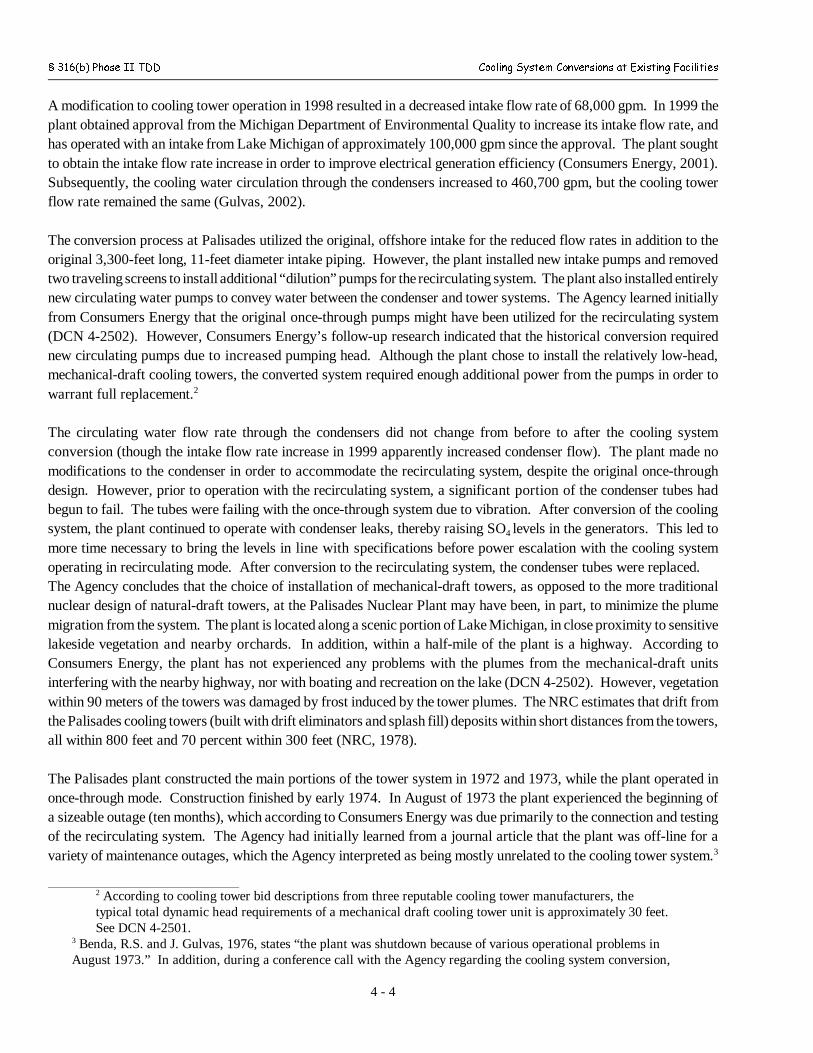
§ 316(b) Phase II TDD Cooling System Conversions at Existing Facilities
2 According to cooling tower bid descriptions from three reputable cooling tower manufacturers, thetypical total dynamic head requirements of a mechanical draft cooling tower unit is approximately 30 feet. See DCN 4-2501.
3 Benda, R.S. and J. Gulvas, 1976, states “the plant was shutdown because of various operational problems inAugust 1973.” In addition, during a conference call with the Agency regarding the cooling system conversion,
4 - 4
A modification to cooling tower operation in 1998 resulted in a decreased intake flow rate of 68,000 gpm. In 1999 theplant obtained approval from the Michigan Department of Environmental Quality to increase its intake flow rate, andhas operated with an intake from Lake Michigan of approximately 100,000 gpm since the approval. The plant soughtto obtain the intake flow rate increase in order to improve electrical generation efficiency (Consumers Energy, 2001).Subsequently, the cooling water circulation through the condensers increased to 460,700 gpm, but the cooling towerflow rate remained the same (Gulvas, 2002).
The conversion process at Palisades utilized the original, offshore intake for the reduced flow rates in addition to theoriginal 3,300-feet long, 11-feet diameter intake piping. However, the plant installed new intake pumps and removedtwo traveling screens to install additional “dilution” pumps for the recirculating system. The plant also installed entirelynew circulating water pumps to convey water between the condenser and tower systems. The Agency learned initiallyfrom Consumers Energy that the original once-through pumps might have been utilized for the recirculating system(DCN 4-2502). However, Consumers Energy’s follow-up research indicated that the historical conversion requirednew circulating pumps due to increased pumping head. Although the plant chose to install the relatively low-head,mechanical-draft cooling towers, the converted system required enough additional power from the pumps in order towarrant full replacement.2
The circulating water flow rate through the condensers did not change from before to after the cooling systemconversion (though the intake flow rate increase in 1999 apparently increased condenser flow). The plant made nomodifications to the condenser in order to accommodate the recirculating system, despite the original once-throughdesign. However, prior to operation with the recirculating system, a significant portion of the condenser tubes hadbegun to fail. The tubes were failing with the once-through system due to vibration. After conversion of the coolingsystem, the plant continued to operate with condenser leaks, thereby raising SO4 levels in the generators. This led tomore time necessary to bring the levels in line with specifications before power escalation with the cooling systemoperating in recirculating mode. After conversion to the recirculating system, the condenser tubes were replaced.The Agency concludes that the choice of installation of mechanical-draft towers, as opposed to the more traditionalnuclear design of natural-draft towers, at the Palisades Nuclear Plant may have been, in part, to minimize the plumemigration from the system. The plant is located along a scenic portion of Lake Michigan, in close proximity to sensitivelakeside vegetation and nearby orchards. In addition, within a half-mile of the plant is a highway. According toConsumers Energy, the plant has not experienced any problems with the plumes from the mechanical-draft unitsinterfering with the nearby highway, nor with boating and recreation on the lake (DCN 4-2502). However, vegetationwithin 90 meters of the towers was damaged by frost induced by the tower plumes. The NRC estimates that drift fromthe Palisades cooling towers (built with drift eliminators and splash fill) deposits within short distances from the towers,all within 800 feet and 70 percent within 300 feet (NRC, 1978).
The Palisades plant constructed the main portions of the tower system in 1972 and 1973, while the plant operated inonce-through mode. Construction finished by early 1974. In August of 1973 the plant experienced the beginning ofa sizeable outage (ten months), which according to Consumers Energy was due primarily to the connection and testingof the recirculating system. The Agency had initially learned from a journal article that the plant was off-line for avariety of maintenance outages, which the Agency interpreted as being mostly unrelated to the cooling tower system.3

§ 316(b) Phase II TDD Cooling System Conversions at Existing Facilities
Consumers Energy stated that operational problems unrelated to the conversion process had been mostlyresponsible for the extended outage (see DCN 4-2502).
4 - 5
However, in a letter submitted to the Agency, Consumers Energy stated, “it appears that the outage was primarily forthe purpose of installing the new circulating water system and the modifications necessary for its operation.” Throughresearch into the historical electricity generation of the plant, the Agency confirms that the outage of ten-monthsoccurred (see DCN 4-2545). However, the Agency notes that it was unable to obtain specific records to show thecause(s) of the outage. The Agency also notes that part of the settlement agreement called for modifications to theradwaste system. In addition, plant operation prior to the conversion had shown problems with the condenser.
The final installed cost of the project was $18.8 million (in 1973-1974 dollars), as paid by Consumers Energy. Thekey items for this project capital cost included the following: two wood cooling towers (including splash fill, drifteliminators, and 36-200 hp fans with 28 ft blades); two circulating water pumps; two dilution water pumps; startuptransformers; yard piping for extension of the plant’s fire protection system; modifications to the plant screenhouse toeliminate travelling screens and prepare for installation of the dilution pumps; a new discharge pump stucture withpump pits; a new pumphouse to enclose the new cooling tower pumps; yard piping for the circulating water system toconnect the new pumphouse and towers; switchgear cubicles for the fans; roads, parking lots, drains, fencing, andlandscaping; and a chemical additive and control system. Additionally, Consumers Energy estimates that the plantabandoned approximately $683,000 (1973/1974 dollars) of original plant equipment. Excluding the sunk costs of theabandoned equipment, the project cost is $58.5 in year 2001 dollars (the cost basis of this proposed rule) or $55.9 inyear 1999 dollars (the dollar basis of facility level cost estimates discussed in Chapter 2 of this document). Frequently,in historical studies of cooling system conversions, the cost basis has been presented as dollars per kW. If the Palisadesconversion project were presented on such a basis, the ratio would be $68 per kW (1999 $ per kW of nameplatecapacity). Utilizing the EPA methodology presented in Chapter 2 for assessing cooling tower “retrofits” gives anestimated installed capital cost of $68 per kW (1999 $) for a nuclear site with the original design characteristics ofPalisades.
The Agency learned that Consumers Energy believes that the cooling tower system at Palisades has a significant impacton the efficiency of the plant’s generating unit. See Chapter 5.6.3 for a discussion of the Palisades estimates of energypenalty impacts from the operation of cooling towers.
Pittsburg Power Plant, Unit 7. Located in Contra Costa County, California, this 751 MW (nameplate, gas-fired steam)unit was originally constructed with a recirculating canal cooling system. The plant began operation in 1972 andconverted to a system with mechanical-draft cooling towers in 1976. The original spray canal system, according toplant personnel, did not operate efficiently enough for the plants needs (DCN 4-2554). The plant then constructed themechanical-draft cooling tower system between two reaches of the original canal. Because of the proximity of thecooling towers to the original circulating piping that serviced the canal, the plant was able to utilize the majority of thisexisting circulating piping system with the converted design. The construction of the cooling towers occurred on a verynarrow strip of land between the canals. The location provides minimal buffer land surrounding the towers, andindicates that the site required significant prepartion work. The cooling towers extend along the canal divider fromabout 300 meters away from the generating unit buildings to approximately 800 meters. The mechanical-draft towersconsist of two units, each with 13 cells. The water supply used in the system is brackish water from Suisun Bay. Thecooling system conversion utilized the existing condenser in addition to the conduit system. The design condenser flowis 352,000 gpm. The plant’s design intake flow rate is 20,200 gpm (EEI, 1994).

§ 316(b) Phase II TDD Cooling System Conversions at Existing Facilities
4 - 6
Pacific Gas & Electric, former owners of the Pittsburg Power Plant, reported the total project cost for the coolingconversion at Pittsburg Unit 7 as $16.7 million (1976 $) (DCN 4-2506). This corresponds to $40.87 million in 1999dollars or $54 per kW (1999 $ per kW of nameplate capacity). Because the plant is in Contra Costa County,California, the cost of construction in this area may not be representative of other areas of the country. The Oakland,California area has a city construction multiplier of approximately 1.19 according to a cost estimating reference (R.S.Means, 2000). Therefore, the costs for the Pittsburg Unit 7 conversion on a national average basis would beapproximately $34.4 million for total project capital cost (in 1999 $) or $46 per kW (1999 $ per kW of nameplatecapacity). Utilizing the EPA methodology presented in Chapter 2 for assessing cooling tower “retrofits” gives anestimated installed capital cost of $38 per kW (1999 $, national-average cost basis) for a site with the characteristicsof Pittsburg Unit 7.
Dry Cooling Conversion Projects. At the time of this proposal, the Agency is unaware of demonstrated cases ofcooling system conversions involving dry cooling systems for the size of power plants within the scope of this proposedrule. See Appendix D of this document for a discussion of dry cooling systems and their applicability for retrofitdesigns.
4.2 PLANT OUTAGES FOR COOLING SYSTEM CONVERSIONS
For three of the cooling system conversion cases examined above, the Agency obtained information from the plantsregarding the gross outage duration for converting between cooling system types. The duration of the outages reportedto the Agency were 83 hours (gross) for the Jefferies Station, 30 days (gross) for each of the two Canadys conversions,and 10 months (gross) for Palisades Nuclear. The Agency examined historical electricity generation data for theseplants and could infer that these outages did occur. However, due to the historical nature of the projects (that is,conversions that occurred from 10 to 30 years ago), the Agency found the documentation of the engineering aspectsof the conversions to be limited. For the more recent projects – Jefferies and Canadys Unit 3 – the Agency receivedinformation directly from members of the plant staff that participated in, or were employed at the stations during theconversions. For Palisades, the Agency received a significant historical information about the plant, but limitedinformation relating to the specifics of the plant outage for the cooling system conversion.
Based on these limited data points provided to the Agency, conclusions as to the expected duration of outages for avariety of cooling system conversions cannot be conclusively drawn. The only substantial conclusion the Agency canreach is that the gross duration of the outage varies widely, based on the data reported to the Agency, and that thepossibility exists for both extremely short outages and those of extremely long duration. The Agency based theeconomic analysis of the regulatory options summarized in Section 4.3 on a gross outage of one-month per convertedplant. The Agency based this estimate on the information it had received from Jefferies and Canadys stations andresearch into other projections (see below). The Agency did not receive the Palisades information until very late in thedevelopment of this proposed rule. Based on the information provided to the Agency (including the late Palisadessubmission), the estimate of one-month could in some cases over- and others under-estimate the expected outageduration for a cooling system conversion. In addition, there is some evidence that the durations of outages may differbased on fuel type (that is, nuclear versus non-nuclear).
As mentioned above, the Agency researched outage projections from historical 316 demonstrations, where plantsconducted engineering studies as to the duration of the expected outage for a site-specific cooling system conversion.Appendix VIII-3 of the Draft Environmental Impact Statement (DEIS) for Bowline Point, Indian Point 2 & 3, andRoseton Generating Stations (Power Tech Associates, 1999) estimates net outage durations for an evaluation of fourclosed-cycle cooling projects. The DEIS states, “plants must be shut down for construction and commissioning beyond

§ 316(b) Phase II TDD Cooling System Conversions at Existing Facilities
4 - 7
the normal shutdowns of the plants. In the cases of Roseton and Bowline, this period was estimated at one monthbeyond normal outages.” For the two nuclear units of Indian Point, the authors estimate two outages for each unit, witheach outage lasting 4 months. The DEIS states that the basis of the longer estimates for the nuclear plants is as follows:“the safety issues have to be addressed during excavation (particularly when blasting is required), tying the new systeminto the plant, and the extensive testing which must follow.” The DEIS estimates that the separate blasting and tying-inoutages would last four months each, considerably longer than for the fossil-fueled Bowline Point and Roseton Stations.The Agency notes that there is no detailed engineering basis (such as detailed descriptions of the types of connectionsto be made, etc.) given by the Authors for any of the projections made in Appendix VIII-3 of the 1999 DEIS.
The Agency also consulted a detailed historical proposal for a Roseton Generating Station cooling system conversion(Central Hudson Gas & Electric, 1977). The report estimates a gross outage period of one-month for the final pipeconnections for the recirculating system. The report estimates the net outage as 10 days for one of the two units andno downtime for the second. The reason for the short estimates of downtime are due to the coincidence of theconnection process with planned winter maintenance outages. Unlike the projection in the 1999 DEIS described above,this 1977 projection was accompanied by a relatively detailed description of the expected level of effort and engineeringexpectations for connecting the reciruclating system to existing equipment.
The Agency learned from the NPDES permit application for Salem Generating Station estimates that outages due toconstruction and conversion to cooling towers are expected to last 7 months per generating unit, in addition to thestation’s planned outages for refueling (see Appendix F, Attachment 8 of the 1999 PSE&G Permit Application forSalem Generating Station, Permit No. NJ0005622).
In addition, the Agency consulted a variety of sources to determine the typical occurrence and duration of plannedmaintenance outages. As noted in the example cases described in Section 4.1 above, each of the cooling systemconversions coincided with planned maintenance outages. Appendix VIII-2.A of the DEIS for the fossil-fuel RosetonStation states, “a review of historical data indicates that there has[sic] been 30 day maintenance outages occurringnominally from mid-Sept. to mid-Oct.”
The 1999 Permit Application for Salem predicts a three year refueling cycle for each unit that is accompanied byoutages of approximately 60 days one year, 40 days in a second year, and no outage in the third. This data is consistentwith other information the Agency obtained from literature. The Agency learned that for 2000 the industry meannuclear refueling outage was approximately 40 days (Nucleonics Week, January 18, 2001). In addition, NUREG-1437shows that nuclear plants undergo periodic and predictable outages for inspections. The following excerpts fromNUREG-1437 explain the NRC’s view of outages at nuclear plants:
From Section 2.2.6-Nuclear power plants must periodically discontinue the production of electricity for refueling, periodic in-service inspection (ISI), and scheduled maintenance. Refueling cycles occur approximately every 12 to 18months. The duration of a refueling outage is typically on the order of 2 months. Enhanced or expandedinspection and surveillance activities are typically performed at 5- and 10-year intervals. These enhancedinspections are performed to comply with Nuclear Regulatory Commission (NRC) and/or industry standardsor requirements such as the American Society of Mechanical Engineers Boiler and Pressure Vessel Code. Five-year ISIs are scheduled for the 5th, 15th, 25th, and 35th years of operation, and 10-year ISIs are performedin the 10th, 20th, and 30th years. Each of these outages typically requires 2 to 4 months of down time for the
§ 316(b) Phase II TDD Cooling System Conversions at Existing Facilities
4 - 8
plant. For economic reasons, many of these activities are conducted simultaneously (e.g., refueling activitiestypically coincide with the ISI and maintenance activities).
Many plants also undertake various major refurbishment activities during their operational lives. Theseactivities are performed to ensure both that the plant can be operated safely and that the capacity and reliabilityof the plant remain at acceptable levels. Typical major refurbishments that have occurred in the past includereplacing PWR steam generators, replacing BWR recirculation piping, and rebuilding main steam turbinestages. The need to perform major refurbishments is highly plant-specific and depends on factors such as designfeatures, operational history, and construction and fabrication details. The plants may remain out of servicefor extended periods of time, ranging from a few months to more than a year, while these major refurbishmentsare accomplished. Outage durations vary considerably, depending on factors such as the scope of the repairsor modifications undertaken, the effectiveness of the outage planning, and the availability of replacement partsand components.
Each nuclear power plant is part of a utility system that may own several nuclear power plants, fossil-firedplants, or other means of generating electricity. An on-site staff is responsible for the actual operation of eachplant, and an off-site staff may be headquartered at the plant site or some other location. Typically, from 800to 2300 people are employed at nuclear power plant sites during periods of normal operation, depending on thenumber of operating reactors located at a particular site. The permanent on-site work force is usually in therange of 600 to 800 people per reactor unit. However, during outage periods, the on-site work force typicallyincreases by 200 to 900 additional workers. The additional workers include engineering support staff,technicians, specialty craftspersons, and laborers called in both to perform specialized repairs, maintenance,tests, and inspections and to assist the permanent staff with the more routine activities carried out during plant
outages.
License renewal schedule and outage periods considered for environmental impact initiator definition,
§ 316(b) Phase II TDD Cooling System Conversions at Existing Facilities
4 - 9
Figure 2.3 from NUREG-1437, Volume I.
The Agency also found information on outage information contained in the April, 2001 accounting report for Mirant,Corp. (form 8K, April 27, 2001). The report gave the following information on planned outages at Mirant’s Californiafossil-fueled power plants:
Major maintenance is presently scheduled on a three-year cycle for the boilers and a 6-year interval for thesteam turbine-generators. The overhaul duration is typically six to eight weeks, depending on the scope of thework to be performed. Virtually all of the Mirant California Facilities' major maintenance for the next fewyears will be performed during outages dictated by the installation of SCR systems or low-NO(X) burners, bothto reduce NO(X) emissions.
Major outages are scheduled for Contra Costa Units 6 and 7 in 2000-2001 to install systems to reduce stackemissions. Low-NO(X) burners were recently installed on Contra Costa Unit 6. Contra Costa Unit 7 isscheduled for installation of a SCR system from March to June of 2001 with Contra Costa Unit 6 SCRinstallation scheduled for 2003.
Major outages are scheduled for Pittsburg Units 1 through 7 within the next three years to install systems toreduce stack emissions or correct equipment concerns that are affecting reliability. Pittsburg Units 1 through4 will retube the condensers and perform boiler repair work in 2001. Pittsburg Units 5 and 6 just completedinstallation of low-NO(X) burners and are scheduled to install SCRs in 2001-2002. Pittsburg Unit 7 isscheduled to install an SCR in 2003. The SCR outages will be between 14 and 20 weeks long.
Potrero Unit 3 will have two major outages in the next four years, 2001 to retube the condenser and make boilerrepairs as necessary and 2004 to install an SCR. The scheduled duration of these outages is 10 and 20 weeksrespectively.
The Agency located a reference for a project where four condenser waterboxes and tube bundles were removed andreplaced at a large nuclear plant (Arkansas Nuclear One). The full project lasted approximately 2 days. The facility,based on experience, had estimated the full condenser replacement to occur over the course of 8 days. Even though thescope of condenser replacements differ from potential cooling system conversions, the regulatory options consideredfor flow reduction commensurate with wet cooling anticipate that a subset of conversions would precipitate condensertube replacements. As such, the condenser replacement schedule is important to the consideration of select coolingsystem conversions.
4.3 SUMMARY OF FLOW-REDUCTION OPTIONS CONSIDERED
The Agency examined regulatory options based on intake flow reduction at in-scope, existing power plants for theproposed rule. The following summaries describe the three wet cooling based options considered by the Agency.
Intake Capacity Commensurate with Closed-Cycle, Recirculating Cooling System for All Facilities
EPA considered a regulatory option that would require Phase II existing facilities having a design intake flow 50MGD or more to reduce the total design intake flow to a level, at a minimum, commensurate with that which can beattained by a closed-cycle recirculating cooling system using minimized make-up and blowdown flows. In addition,
§ 316(b) Phase II TDD Cooling System Conversions at Existing Facilities
4 - 10
facilities in specified circumstances (for example, located where additional protection is needed due to concernsregarding threatened, endangered, or protected species or habitat; migratory, sport or commercial species ofconcern) would have to select and implement design and construction technologies to minimize impingementmortality and entrainment. This option does not distinguish between facilities on the basis of the waterbody fromwhich they withdraw cooling water. Rather, it would ensure that the same stringent controls are the nationallyapplicable minimum for all waterbody types. This is the regulatory approach EPA adopted for new facilities. Asstated above, 73 of the facilities potentially subject to this proposed rule already utilize a recirculating wet coolingsystem (e.g., wet cooling towers or ponds). These facilities would meet the requirements under this option unlessthey are located in areas where the director or fisheries managers determine that fisheries need additional protection. Therefore, under this option, 466 steam electric power generating facilities would be required to meet performancestandards for reducing impingement mortality and entrainment based on a reduction in intake flow to a levelcommensurate with that which can be attained by a recirculating, closed-cycle wet system.
EPA did not select closed-cycle, recirculating cooling systems as the best technology available for existing facilitiesbecause of the generally high costs of such conversions. According to EPA’s cost estimates, capital costs forindividual high-flow plants to convert to wet towers generally ranged from 130 to 200 million dollars, with annualoperating costs in the range of 4 to 20 million dollars. EPA estimates that the total annualized post-tax cost ofcompliance for this option is approximately $2.26 billion. Not included in this estimate are 9 facilities that areprojected to be baseline closures. Including compliance costs for these 9 facilities would increase the total cost ofcompliance with this option to approximately $2.32 billion. EPA also has serious concerns about the short-termenergy implications of a massive concurrent conversion and the potential for supply disruptions that it would entail.
The estimated annual benefits (in $2001) for requiring all Phase II existing facilities to reduce intake capacitycommensurate with the use of closed-cycle, recirculating cooling systems are $83.9 million per year and $1.08billion for entrainment reductions.
Intake Capacity Commensurate with Closed-Cycle Wet Cooling Systems for All Facilities on Oceans,Estuaries, and Tidal Rivers
EPA considered an alternate technology-based option in which closed-cycle, recirculating cooling systems would berequired for all facilities on certain waterbody types. Under this option, EPA would group waterbodies into thesame five categories as in today’s proposal: (1) freshwater rivers or streams, (2) lakes or reservoirs, (3) GreatLakes, (4) tidal rivers or estuaries; and (5) oceans. Because oceans, estuaries and tidal rivers contain essentialhabitat and nursery areas for the vast majority of commercial and recreational important species of shell and finfish, including many species that are subject to intensive fishing pressures, these waterbody types would requiremore stringent controls based on the performance of closed-cycle, recirculating cooling systems. EPA discussed thesusceptibility of these waters in a Notice of Data Availability (NODA) for the new facility rule (66 FR 28853, May25, 2001) and invited comment on documents that may support its judgment that these waters are particularlysusceptible to adverse impacts from cooling water intake structures. In addition, the NODA presented informationregarding the low susceptibility of non-tidal freshwater rivers and streams to impacts from entrainment fromcooling water intake structures. Under this alternative option, facilities that operate at less than 15 percent capacity utilization would, as in theproposed option, only be required to have impingement control technology. Facilities that have a closed-cycle,recirculating cooling system would require additional design and construction technologies to increase the survival
§ 316(b) Phase II TDD Cooling System Conversions at Existing Facilities
4 - 11
rate of impinged biota or to further reduce the amount of entrained biota if the intake structure was located withinan ocean, tidal river, or estuary where there are fishery resources of concern to permitting authorities or fisherymanagers.
Facilities with cooling water intake structures located in a freshwater (including rivers and streams, the Great Lakesand other lakes) would have the same requirements as under the proposed rule. If a facility chose to comply withTrack II, then the facility would have to demonstrate that alternative technologies would reduce impingement andentrainment to levels comparable to those that would be achieved with a closed-loop recirculating system (90%reduction). If such a facility chose to supplement its alternative technologies with restoration measures, it wouldhave to demonstrate the same or substantially similar level of protection. (For additional discussion see the newfacility final rule 66 FR 65256, at 65315 columns 1 and 2.)
EPA has estimated that there are 109 facilities located on oceans, estuaries, or tidal rivers that do not have a closedcycle recirculating system and would be required to meet performance standards for reducing impingementmortality and entrainment based on a reduction in intake flow to a level commensurate with that which can beattained by a closed-cycle recirculating system. The other 430 facilities would be required to meet the sameperformance standards in the in today’s proposal.
The potential environmental benefits of this option have been estimated at $87.8 million and $1.24 billion forentrainment reductions annually. Although this option is estimated (a full cost analysis was not done for this option)to be less expensive at a national level than requiring closed-cycle, recirculating cooling systems for all Phase IIexisting facilities, EPA is not proposing this option. Facilities located on oceans, estuaries, and tidal rivers wouldincur high capital and operating and maintenance costs for conversions of their cooling water systems. Furthermore, since impacted facilities would be concentrated in coastal regions, there is the potential for short-termenergy impacts and supply disruptions in these areas. EPA also invites comment on this option.
Intake Capacity Commensurate with Closed-Cycle, Recirculating Cooling System Based on Waterbody Type
EPA also considered a variation on the above approach that would require only facilities withdrawing very largeamounts of water from an estuary, tidal river, or ocean to reduce their intake capacity to a level commensurate withthat which can be attained by a closed-cycle, recirculating cooling system.
For example, for facilities with cooling water intake structures located in a tidal river or estuary, if the intake flowis greater than 1 percent of the source water tidal excursion, then the facility would have to meet standards forreducing impingement mortality and entrainment based on the performance of wet cooling towers. These facilitieswould have the choice of complying with Track I or Track II requirements. If a facility on a tidal river or estuaryhas intake flow equal to or less than 1 percent of the source water tidal excursion, the facility would only berequired to meet the performance standards in the proposed rule. These standards are based on the performance oftechnologies such as fine mesh screens and traveling screens with well-designed and operating fish return systems.The more stringent, closed-cycle, recirculating cooling system-based requirements would also apply to a facilitythat has a cooling water intake structure located in an ocean with an intake flow greater than 500 MGD.
§ 316(b) Phase II TDD Cooling System Conversions at Existing Facilities
4 - 12
REFERENCES
Benda, R.S. and J. Gulvas, 1976, “Effects of Palisades Nuclear Power Plant on Lake Michigan,” Thermal EcologyII, Proceedings of a Symposium Held at Augusta, Georgia.
Central Hudson Gas & Electric Corporation, 1977, “Engineering, Environmental (Nonbiological), and EconomicAspects of a Closed-Cycle Cooling System,” Roseton Generating Station.
Consumers Energy Company and Nuclear Management Corporation, May 2001, “Biological Assessment of the1999 Cooling Water Flow Increase at the Palisades Nuclear Plant, near South Haven, Michigan.”
Edison Electric Institute, 1994, “Power Statistics Unit Design Data File Part B of the 1994 UDI Database.”
Gulvas, J.A., Consumers Energy, Feb. 28, 2002, Data Submission to Tim Connor of the U.S. EPA, “RE: PalisadesPlant Once-Through and Cooling Towers.”
Henderson, J., Santee Cooper, 2002, Response to Information Request from Tim Connor of USEPA. (DCN 4-2528)
Platts, 2001, “U.S. Utilities Reporting Record 2000 Nuclear Output,” Nucleonics Week, Vol. 42 No. 3, January18, 2001, McGraw-Hill Companies, Inc.
Mirant Corp., 2001, Form 8K -- April 27, 2001, Item 9. Regulation FD Disclosure. http://www.biz.yahoo.com/e/010427/mir.html
Pearrow, J. J., 2001, “Hydrogen Peroxide Keeps Cooling Tower Fill Clean,” Power Magazine, May/June 2001. (DCN 4-2523)
Perry, W. J., 1991, “Adverse Impact Study, Cooling Water Facilities, Jefferies Generating Station,” MoncksCorner, South Carolina, Santee Cooper.
Power Tech Associates, 1999, “Economic and Environmental Review of Closed Cooling Water Systems for theHudson River Power Plants,” prepared for Central Hudson Gas & Electric, Corp., et al., Appendix VIII-3 of theDraft Environmental Impact Statement for Bowline Point, Indian Point 2 & 3, and Roseton Generating Stations.
United States Nuclear Regulatory Comission, 1978, “Final Adendum to the Final Environmental Statement forPalisades Nuclear Generating Plant,” Docket No. 50-255, Final Adendum to FES (NUREG-0343).
U.S. EPA teleconference with John Gulvas of Consumers Energy; December 2001. (DCN 4-2502)
U.S. EPA, 2002, “Phone Memorandum - Conversation with Ron Kino of Mirant Pittsburg.” (DCN 4-2554)
Veil, J., 2002, Correspondence with US EPA. (DCN 4-2506)
Waier, P. R., Senior Editor, 2000, “R.S. Means Building Construction Cost Data,” 58th Annual Edition, R.S.Means Company, Inc.
Wicker, K., South Carolina Electric & Gas Co., 2002, Response to Information Request from Tim Connor ofUSEPA. (DCN 4-2508)
§ 316(b) Phase II TDD Energy Penalties of Cooling Towers
5 - 1
Chapter 5: Energy Penalties of Cooling Towers
INTRODUCTION
For the Existing Facility 316(b) Proposal, the Agency considered regulatory options in which regulated facilities (ora subset thereof) would achieve flow reduction commensurate with closed-cycle wet cooling systems. In addition, theAgency analyzed regulatory options based on flow reduction commensurate with near-zero intake of dry coolingsystems. This chapter discusses the topics of energy penalties of such cooling systems.
For the Section 316(b) New Facility Final Rule the Agency researched and derived energy penalty estimates, based onempirical data and proven theoretical concepts, for a variety of conditions. The regulatory analysis conducted by theAgency for this Existing Facility Section 316(b) Proposal utilized the results of the New Facility analysis. This chapterpresents the research, methodology, results, and conclusions for the Agency’s thorough effort to estimate energypenalties due to the operational performance of power plant cooling systems.
As a consequence of energy penalties for some cooling systems, increased air pollutant emissions may occur for somepower plants as compared to a baseline system. The discussion of air pollutant emissions and other potentialenvironmental impacts from cooling towers are presented in Chapter 6 of this document.
The remainder of this chapter is organized as follows:
< Section 5.1 presents the energy penalty estimates used for analysis of the flow reduction regulatory options.
< Section 5.2 presents an introduction to the Agency’s energy penalty estimates.
< Section 5.3 focuses on steam turbines and the changes in efficiency associated with using alternative coolingsystems.
< Section 5.4 evaluates the net difference in required pumping and fan energy for alternative cooling systems.
< Section 5.5 combines and summarizes the energy impacts of pumping and fan energy requirements for alternativecooling systems.
< Section 5.6 summarizes data from other sources on the potential energy penalty of alternative cooling systems atexisting facilities.
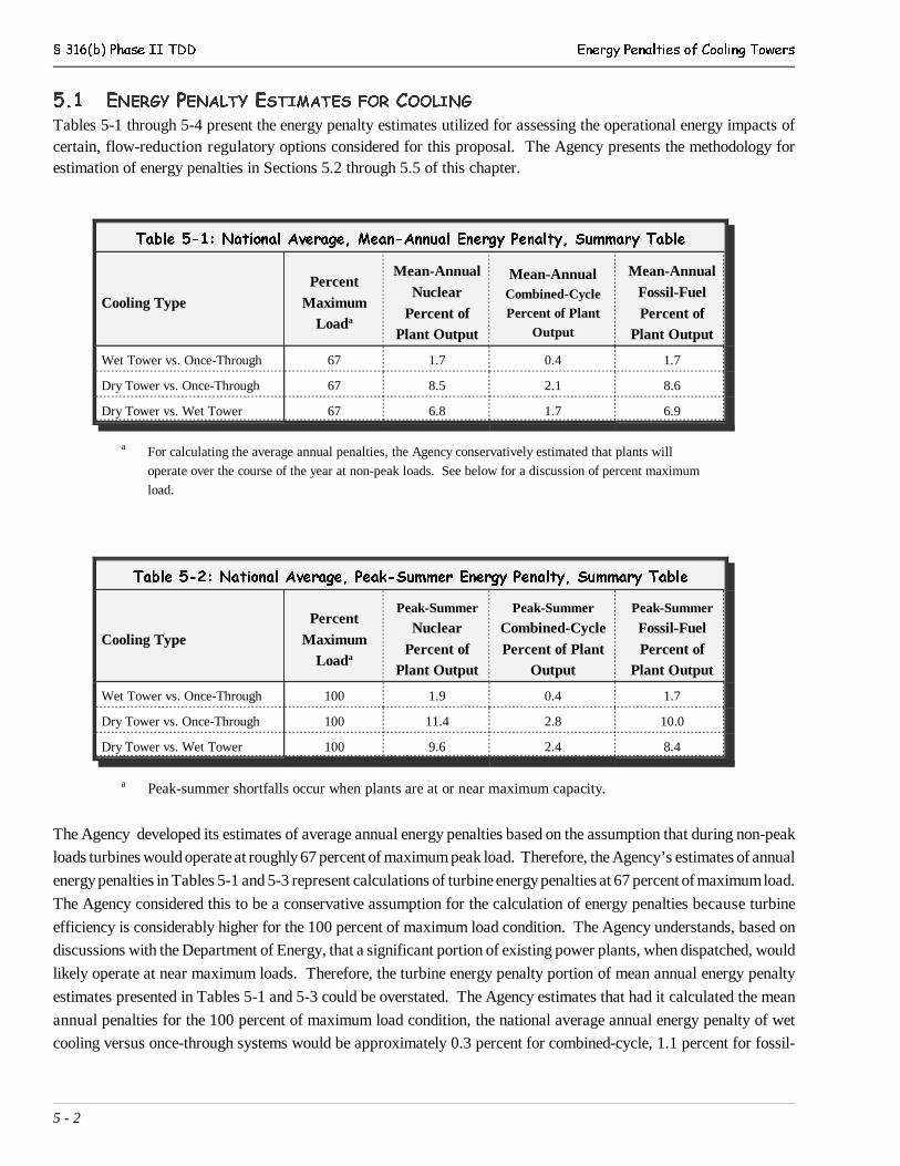
§ 316(b) Phase II TDD Energy Penalties of Cooling Towers
5 - 2
5.1 ENERGY PENALTY ESTIMATES FOR COOLING
Tables 5-1 through 5-4 present the energy penalty estimates utilized for assessing the operational energy impacts ofcertain, flow-reduction regulatory options considered for this proposal. The Agency presents the methodology forestimation of energy penalties in Sections 5.2 through 5.5 of this chapter.
Table 5-1: National Average, Mean-Annual Energy Penalty, Summary Table
Cooling TypePercent
MaximumLoada
Mean-AnnualNuclear
Percent ofPlant Output
Mean-AnnualCombined-CyclePercent of Plant
Output
Mean-AnnualFossil-FuelPercent of
Plant Output
Wet Tower vs. Once-Through 67 1.7 0.4 1.7
Dry Tower vs. Once-Through 67 8.5 2.1 8.6
Dry Tower vs. Wet Tower 67 6.8 1.7 6.9
a For calculating the average annual penalties, the Agency conservatively estimated that plants will
operate over the course of the year at non-peak loads. See below for a discussion of percent maximum
load.
Table 5-2: National Average, Peak-Summer Energy Penalty, Summary Table
Cooling TypePercent
MaximumLoada
Peak-Summer
NuclearPercent of
Plant Output
Peak-Summer
Combined-CyclePercent of Plant
Output
Peak-Summer
Fossil-FuelPercent of
Plant Output
Wet Tower vs. Once-Through 100 1.9 0.4 1.7
Dry Tower vs. Once-Through 100 11.4 2.8 10.0
Dry Tower vs. Wet Tower 100 9.6 2.4 8.4
a Peak-summer shortfalls occur when plants are at or near maximum capacity.
The Agency developed its estimates of average annual energy penalties based on the assumption that during non-peak
loads turbines would operate at roughly 67 percent of maximum peak load. Therefore, the Agency’s estimates of annual
energy penalties in Tables 5-1 and 5-3 represent calculations of turbine energy penalties at 67 percent of maximum load.
The Agency considered this to be a conservative assumption for the calculation of energy penalties because turbine
efficiency is considerably higher for the 100 percent of maximum load condition. The Agency understands, based on
discussions with the Department of Energy, that a significant portion of existing power plants, when dispatched, would
likely operate at near maximum loads. Therefore, the turbine energy penalty portion of mean annual energy penalty
estimates presented in Tables 5-1 and 5-3 could be overstated. The Agency estimates that had it calculated the mean
annual penalties for the 100 percent of maximum load condition, the national average annual energy penalty of wet
cooling versus once-through systems would be approximately 0.3 percent for combined-cycle, 1.1 percent for fossil-
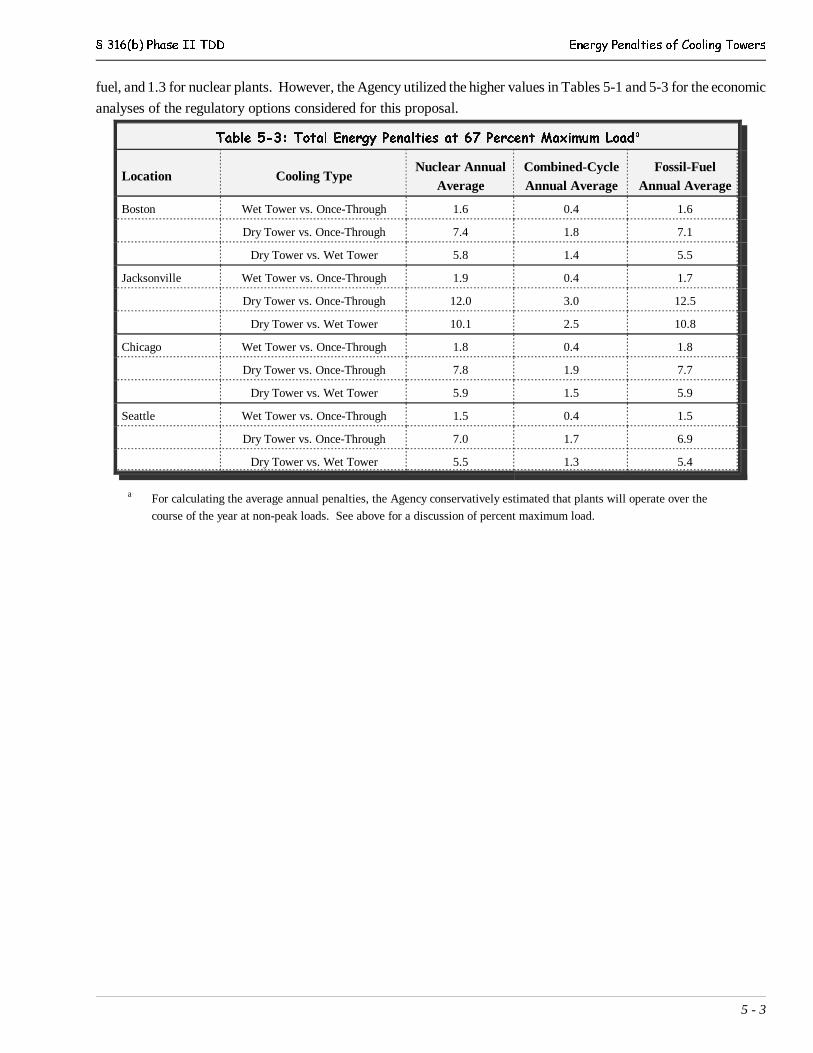
§ 316(b) Phase II TDD Energy Penalties of Cooling Towers
5 - 3
fuel, and 1.3 for nuclear plants. However, the Agency utilized the higher values in Tables 5-1 and 5-3 for the economic
analyses of the regulatory options considered for this proposal.
Table 5-3: Total Energy Penalties at 67 Percent Maximum Loada
Location Cooling TypeNuclear Annual
AverageCombined-CycleAnnual Average
Fossil-FuelAnnual Average
Boston Wet Tower vs. Once-Through 1.6 0.4 1.6
Dry Tower vs. Once-Through 7.4 1.8 7.1
Dry Tower vs. Wet Tower 5.8 1.4 5.5
Jacksonville Wet Tower vs. Once-Through 1.9 0.4 1.7
Dry Tower vs. Once-Through 12.0 3.0 12.5
Dry Tower vs. Wet Tower 10.1 2.5 10.8
Chicago Wet Tower vs. Once-Through 1.8 0.4 1.8
Dry Tower vs. Once-Through 7.8 1.9 7.7
Dry Tower vs. Wet Tower 5.9 1.5 5.9
Seattle Wet Tower vs. Once-Through 1.5 0.4 1.5
Dry Tower vs. Once-Through 7.0 1.7 6.9
Dry Tower vs. Wet Tower 5.5 1.3 5.4
a For calculating the average annual penalties, the Agency conservatively estimated that plants will operate over the
course of the year at non-peak loads. See above for a discussion of percent maximum load.
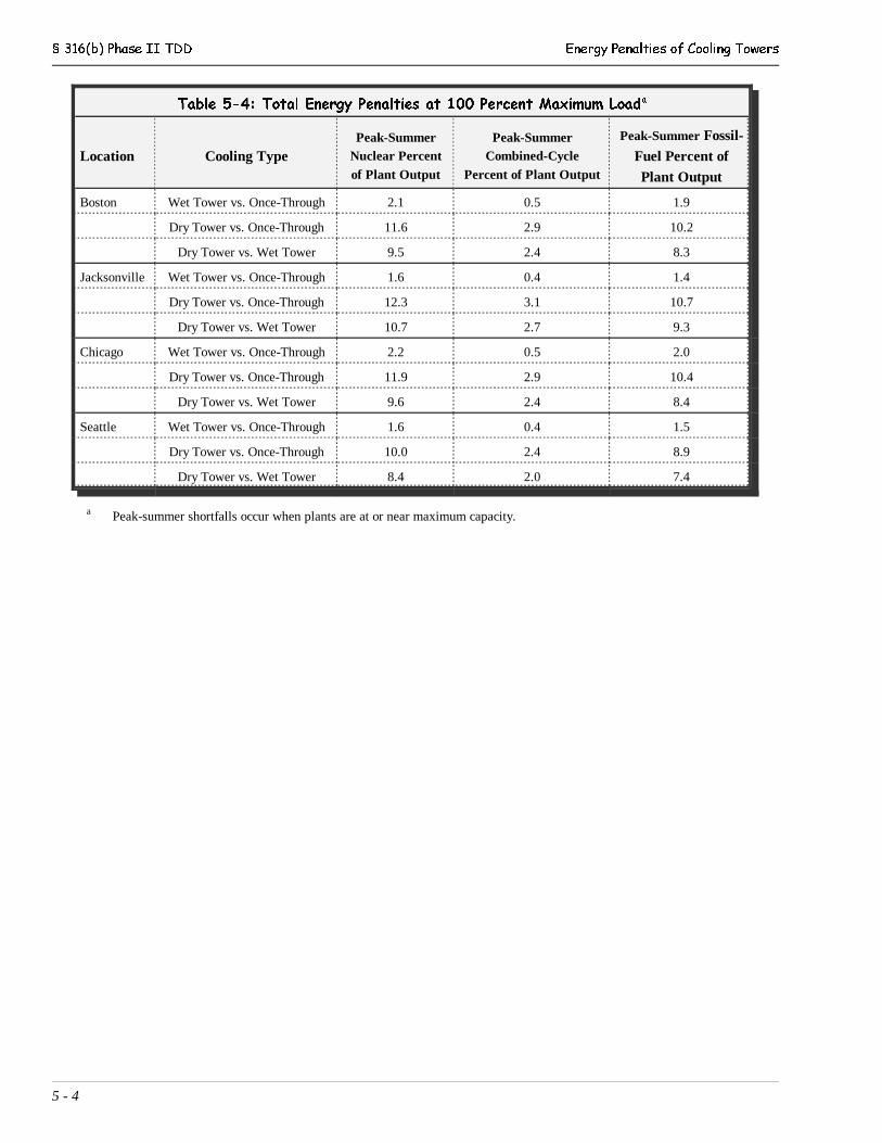
§ 316(b) Phase II TDD Energy Penalties of Cooling Towers
5 - 4
Table 5-4: Total Energy Penalties at 100 Percent Maximum Loada
Location Cooling TypePeak-Summer
Nuclear Percentof Plant Output
Peak-SummerCombined-Cycle
Percent of Plant Output
Peak-Summer Fossil-Fuel Percent ofPlant Output
Boston Wet Tower vs. Once-Through 2.1 0.5 1.9
Dry Tower vs. Once-Through 11.6 2.9 10.2
Dry Tower vs. Wet Tower 9.5 2.4 8.3
Jacksonville Wet Tower vs. Once-Through 1.6 0.4 1.4
Dry Tower vs. Once-Through 12.3 3.1 10.7
Dry Tower vs. Wet Tower 10.7 2.7 9.3
Chicago Wet Tower vs. Once-Through 2.2 0.5 2.0
Dry Tower vs. Once-Through 11.9 2.9 10.4
Dry Tower vs. Wet Tower 9.6 2.4 8.4
Seattle Wet Tower vs. Once-Through 1.6 0.4 1.5
Dry Tower vs. Once-Through 10.0 2.4 8.9
Dry Tower vs. Wet Tower 8.4 2.0 7.4
a Peak-summer shortfalls occur when plants are at or near maximum capacity.
§ 316(b) Phase II TDD Energy Penalties of Cooling Towers
5 - 5
5.2 INTRODUCTION TO ENERGY PENALTY ESTIMATES
This energy penalty discussion presents differences in steam power plant efficiency or output associated with the effectof using alternative cooling systems. In particular, this evaluation focuses on power plants that use steam turbines andthe changes in efficiency associated with using alternative cooling systems. The cooling systems evaluated include:once-through cooling systems; wet tower closed-cycle systems; and direct-dry cooling systems using air cooledcondensers. However, the methodology is flexible and can be extended to other alternative types of cooling systemsso long as the steam condenser performance or the steam turbine exhaust pressure can be estimated.
The energy penalties presented in this chapter were developed for new, “greenfield” facilities. As such, the Agencyestimates for this proposal for existing facilities that the energy penalties of cooling system conversions from once-through to recirculating wet cooling towers would be similar to the new, “greenfield” cases. The Department of Energyexpressed concern that this methodology may underestimate the pumping energy requirements of recirculating wet towersystems for converted cooling systems. This matter, among others, is discussed in Section 5.6 below.
The Agency acknowledges that direct-dry cooling systems are unlikely candidates for cooling system conversions atexisting power plants. A direct-dry cooling system (as discussed in Appendix D of this document) condenses theexhaust steam that is fed directly to the dry tower from the generating turbine. However, steam turbines at the existingpower plants within the scope of this rule are, without exception, configured to condense steam utilizing a surfacecondenser system. Therefore, the only type of dry cooling system that would be considered for a cooling systemconversion is an indirect-air cooled condenser. Otherwise, the entire steam turbine would be replaced or dramaticallyreconfigured to feed exhaust steam to a direct-dry cooling system. The engineering feasibility of this type of plantreconfiguration was considered unproven by the Agency and the costs of turbine replacement were also deemed too highfor this proposal.
Indirect-dry cooling systems operate less efficiently than direct-dry cooled systems. Therefore, the energy penalties fordry cooling systems presented in this chapter would be higher for the only application that would be considered forexisting facilities. The Department of Energy (DOE) studied the peak summer energy penalty resulting from convertingplants with once-through cooling to wet towers or indirect dry towers (see DCN 4-2512). DOE modeled five locations– Delaware River Basin (Philadelphia), Michigan/Great Lakes (Detroit), Ohio River Valley (Indianapolis), South(Atlanta), and Southwest (Yuma) – using an ASPEN simulator model. The model evaluated the performance andenergy penalty for hypothetical 400-MW coal-fired plants that were retrofitted from using once-through cooling systemsto wet- and dry-recirculating systems. The DOE estimates that conversion to an indirect-dry tower could cause peaksummer energy penalties ranging from 8.9 percent to 14.1 percent with a design approach of 20 degrees Fahrenheit and12.7 percent to approximately 18 percent with an approach of 40 degrees Fahrenheit. Note that these peak summerenergy penalties are higher than those estimated by EPA (as presented in Tables 5-2 and 5-4 above) for the direct-drycooling system. The Agency’s estimates of direct-dry cooling system peak summer energy penalties range from 7.4percent to 10.7 percent for fossil-fuel plants. As such, the analysis of energy effects of the dry cooling-based regulatoryoptions considered for this proposal may not reflect the full magnitude of the energy penalty of the indirect-dry coolingsystems.
5.2.1 Power Plant Efficiencies
Most power plants that use a heat-generating fuel as the power source use a steam cycle referred to as a “RankineEngine,” in which water is heated into steam in a boiler and the steam is then passed through a turbine (Woodruff1998). After exiting the turbine, the spent steam is condensed back into water and pumped back into the boiler to repeatthe cycle. The turbine, in turn, drives a generator that produces electricity. As with any system that converts energy
§ 316(b) Phase II TDD Energy Penalties of Cooling Towers
5 - 6
from one form to another, not all of the energy available from the fuel source can be converted into useful energy in apower plant.
Steam turbines extract power from steam as the steam passes from high pressure and high temperature conditions atthe turbine inlet to low pressure and lower temperature conditions at the turbine outlet. Steam exiting the turbine goesto the condenser, where it is condensed to water. The condensation process is what creates the low pressure conditionsat the turbine outlet. The steam turbine outlet or exhaust pressure (which is often a partial vacuum) is a function ofthe temperature maintained at the condensing surface (among other factors) and the value of the exhaust pressure canhave a direct effect on the energy available to drive the turbine. The lower the exhaust pressure, the greater the amountof energy that is available to drive the turbine, which in turn increases the overall efficiency of the system since noadditional fuel energy is involved.
The temperature of the condensing surface is dependent on the design and operating conditions within the condensingsystem (e.g., surface area, materials, cooling fluid flow rate, etc.) and especially the temperature of the cooling wateror air used to absorb heat and reject it from the condenser. Thus, the use of a different cooling system can affect thetemperature maintained at the steam condensing surface (true in many circumstances). This difference can result ina change in the efficiency of the power plant. These efficiency differences vary throughout the year and may be morepronounced during the warmer months. Equally important is the fact that most alternative cooling systems will requirea different amount of power to operate equipment such as fans and pumps, which also can have an effect on the overallplant energy efficiency. The reductions in energy output resulting from the energy required to operate the coolingsystem equipment are often referred to as parasitic losses.
In general, the penalty described here is only associated with power plants that utilize a steam cycle for powerproduction. Therefore, this analysis will focus only on steam turbine power plants and combined-cycle gas plants. Themost common steam turbine power plants are those powered by steam generated in boilers heated by the combustionof fossil fuels or by nuclear reactors.
Combined-cycle plants use a two-step process in which the first step consists of turbines powered directly by highpressure hot gases from the combustion of natural gas, oil, or gasified coal. The second step consists of a steam cyclein which a turbine is powered by steam generated in a boiler heated by the low pressure hot gases exiting the gasturbines. Consequently, the combined-cycle plants have much greater overall system efficiencies. However, the energypenalty associated with using alternative cooling systems is only associated with the steam cycle portion of the system.Because steam plants cannot be quickly started or stopped, they often operate as base load plants, which arecontinuously run to serve the minimum load required by the system. Since combined-cycle plants obtain only a portionof their energy from the slow-to-start/stop steam power step, the inefficiency of the start-up/stop time period is moreeconomically acceptable and therefore they are generally used for intermediate loads. In other words, they are startedand stopped at a greater frequency and with greater efficiency than base load steam plant facilities.
One measure of the plant thermal efficiency used by the power industry is the Net Plant Heat Rate (NPHR), which isthe ratio of the total fuel heat input (BTU/hr) divided by the net electric generation (kW). The net electric generationincludes only electricity that leaves the plant. The total energy plant efficiency can be calculated from the NPHR usingthe following formula:
Plant Energy Efficiency = 3413 / NPHR x 100 (1)
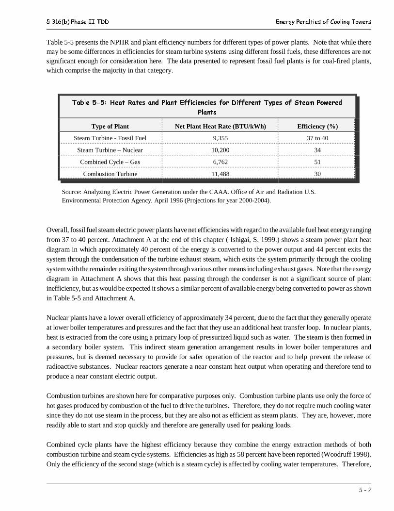
§ 316(b) Phase II TDD Energy Penalties of Cooling Towers
5 - 7
Table 5-5 presents the NPHR and plant efficiency numbers for different types of power plants. Note that while theremay be some differences in efficiencies for steam turbine systems using different fossil fuels, these differences are notsignificant enough for consideration here. The data presented to represent fossil fuel plants is for coal-fired plants,which comprise the majority in that category.
Table 5-5: Heat Rates and Plant Efficiencies for Different Types of Steam Powered
Plants
Type of Plant Net Plant Heat Rate (BTU/kWh) Efficiency (%)
Steam Turbine - Fossil Fuel 9,355 37 to 40
Steam Turbine – Nuclear 10,200 34
Combined Cycle – Gas 6,762 51
Combustion Turbine 11,488 30
Source: Analyzing Electric Power Generation under the CAAA. Office of Air and Radiation U.S.Environmental Protection Agency. April 1996 (Projections for year 2000-2004).
Overall, fossil fuel steam electric power plants have net efficiencies with regard to the available fuel heat energy rangingfrom 37 to 40 percent. Attachment A at the end of this chapter ( Ishigai, S. 1999.) shows a steam power plant heatdiagram in which approximately 40 percent of the energy is converted to the power output and 44 percent exits thesystem through the condensation of the turbine exhaust steam, which exits the system primarily through the coolingsystem with the remainder exiting the system through various other means including exhaust gases. Note that the exergydiagram in Attachment A shows that this heat passing through the condenser is not a significant source of plantinefficiency, but as would be expected it shows a similar percent of available energy being converted to power as shownin Table 5-5 and Attachment A.
Nuclear plants have a lower overall efficiency of approximately 34 percent, due to the fact that they generally operateat lower boiler temperatures and pressures and the fact that they use an additional heat transfer loop. In nuclear plants,heat is extracted from the core using a primary loop of pressurized liquid such as water. The steam is then formed ina secondary boiler system. This indirect steam generation arrangement results in lower boiler temperatures andpressures, but is deemed necessary to provide for safer operation of the reactor and to help prevent the release ofradioactive substances. Nuclear reactors generate a near constant heat output when operating and therefore tend toproduce a near constant electric output.
Combustion turbines are shown here for comparative purposes only. Combustion turbine plants use only the force ofhot gases produced by combustion of the fuel to drive the turbines. Therefore, they do not require much cooling watersince they do not use steam in the process, but they are also not as efficient as steam plants. They are, however, morereadily able to start and stop quickly and therefore are generally used for peaking loads.
Combined cycle plants have the highest efficiency because they combine the energy extraction methods of bothcombustion turbine and steam cycle systems. Efficiencies as high as 58 percent have been reported (Woodruff 1998).Only the efficiency of the second stage (which is a steam cycle) is affected by cooling water temperatures. Therefore,
§ 316(b) Phase II TDD Energy Penalties of Cooling Towers
5 - 8
for the purposes of this analysis, the energy penalty for combined cycle plants is applicable only to the energy outputof the steam plant component, which is generally reported to be approximately one-third of the overall combined-cycleplant energy output.
5.3 TURBINE EFFICIENCY ENERGY PENALTY
5.3.1 Effect of Turbine Exhaust Pressure
The temperature of the cooling water (or air in air-cooled systems) entering the steam cycle condensers affects theexhaust pressure at the outlet of the turbine. In general, a lower cooling water or air temperature at the condenser inletwill result in a lower turbine exhaust pressure. Note that for a simple steam turbine, the available energy is equal tothe difference in the enthalpy of the inlet steam and the combined enthalpy of the steam and condensed moisture at theturbine outlet. A reduction in the outlet steam pressure results in a lower outlet steam enthalpy. A reduction in theenthalpy of the turbine exhaust steam, in combination with an increase in the partial condensation of the steam, resultsin an increase in the efficiency of the turbine system. Of course, not all of this energy is converted to the torque energy(work) that is available to turn the generator, since steam and heat flow through the turbine systems is complex withvarious losses and returns throughout the system.
The turbine efficiency energy penalty as described below rises and drops in direct response to the temperature of thecooling water (or air in air-cooled systems) delivered to the steam plant condenser. As a result, it tends to peak duringthe summer and may be substantially diminished or not exist at all during other parts of the year.
The design and operation of the steam condensing system can also affect the system efficiency. In general, design andoperational changes that improve system efficiency such as greater condenser surface areas and coolant flow rates willtend to result in an increase in the economic costs and potentially the environmental detriments of the system. Thus,the design and operation of individual systems can differ depending on financial decisions and other site-specificconditions. Consideration of such site-specific design variations is beyond the scope of this evaluation. Therefore,conditions that represent a typical, or average, system derived from available information for each technology will beused. However, regional and annual differences in cooling fluid temperatures are considered. Where uncertainty exists,a conservative estimate is used. In this context, conservative means the penalty estimate is biased toward a higher value.
Literature sources indicate that condenser inlet temperatures of 55 °F and 95 °F will produce turbine exhaust pressuresof 1.5 and 3.5 inches Hg, respectively, in a typical surface condenser (Woodruff 1998). If the turbine steam inletconditions remain constant, lower turbine exhaust pressures will result in greater changes in steam enthalpy betweenthe turbine inlet and outlet. This in turn will result in higher available energy and higher turbine efficiencies. The lower outlet pressures can also result in the formation of condensed liquid water within the low pressure end of theturbine. Note that liquid water has a significantly lower enthalpy value which, based on enthalpy alone, should resultin even greater turbine efficiencies. However, the physical effects of moisture in the turbines can cause damage to theturbine blades and can result in lower efficiencies than would be expected based on enthalpy data alone. This damageand lower efficiency is due to the fact that the moisture does not follow the steam path and impinges upon the turbineblades. More importantly, as the pressure in the turbine drops, the steam volume increases. While the turbines aredesigned to accommodate this increase in volume through a progressive increase in the cross-sectional area, economicconsiderations tend to limit the size increase such that the turbine cannot fully accommodate the expansion that occursat very low exhaust pressures.
Thus, for typical turbines, as the exhaust pressure drops below a certain level, the increase in the volume of the steamis not fully accommodated by the turbine geometry, resulting in an increase in steam velocity near the turbine exit. This
§ 316(b) Phase II TDD Energy Penalties of Cooling Towers
5 - 9
increase in steam velocity results in the conversion of a portion of the available steam energy to kinetic energy, thusreducing the energy that could otherwise be available to drive the turbine. Note that kinetic energy is proportional tothe square of the velocity. Consequently, as the steam velocity increases, the resultant progressive reduction in availableenergy tends to offset the gains in available energy that would result from the greater enthalpy changes due to thereduced pressure. Thus, the expansion of the steam within the turbine and the formation of condensed moistureestablishes a practical lower limit for turbine exhaust pressures, reducing the efficiency advantage of even lowercondenser surface temperatures particularly at higher turbine steam loading rates. As can be seen in the turbineperformance curves presented below, this reduction in efficiency at lower exhaust pressures is most pronounced athigher turbine steam loading rates. This is due to the fact that higher steam loading rates will produce proportionatelyhigher turbine exit velocities.
Attachment B presents several graphs showing the change in heat rate resulting from differences in the turbine exhaustpressure at a nuclear power plant, a fossil fueled power plant, and a combined-cycle power plant (steam portion). Thefirst graph (Attachment B-1) is for a GE turbine and was submitted by the industry in support of an analysis for anuclear power plant. The second graph (Attachment B-2) is from a steam turbine technical manual and is for a turbineoperating at steam temperatures and pressures consistent with a sub-critical fossil fuel plant (2,400 psig, 1,000 °F).The third graph (Attachment B-3) is from an engineering report analyzing operational considerations and design ofmodifications to a cooling system for a combined-cycle power plant.
The changes in heat rate shown in the graphs can be converted to changes in turbine efficiency using Equation 1. Several curves on each graph show that the degree of the change (slope of the curve) decreases with increasing loads.Note that the amount of electricity being generated will also vary with the steam loading rates such that the morepronounced reduction in efficiency at lower steam loading rates applies to a reduced power output. The curves alsoindicate that, at higher steam loads, the plant efficiency optimizes at an exhaust pressure of approximately 1.5 inchesHg. At lower exhaust pressures the effect of increased steam velocities actually results in a reduction in overallefficiency. The graphs in Attachment B will serve as the basis for estimating the energy penalty for each type offacility.
Since the turbine efficiency varies with the steam loading rate, it is important to relate the steam loading rates to typicaloperating conditions. It is apparent from the heat rate curves in Attachment B that peak loading, particularly if theexhaust pressure is close to 1.5 inches Hg, presents the most efficient and desirable operating condition. Obviously,during peak loading periods, all turbines will be operating near the maximum steam loading rates and the energy penaltyderived from the maximum loading curve would apply. It is also reasonable to assume that power plants that operateas base load facilities will operate near maximum load for a majority of the time they are operating. However, therewill be times when the power plant is not operating at peak capacity. One measure of this is the capacity factor, whichis the ratio of the average load on the plant over a given period to its total capacity. For example, if a 200 MW plantoperates, on average, at 50 percent of capacity (producing an average of 100 MW when operating) over a year, thenits capacity factor would be 50 percent.
The average capacity factor for nuclear power plants in the U.S. has been improving steadily and recently has beenreported to be approximately 89 percent. This suggests that for nuclear power plants, the majority appear to beoperating near capacity most of the time. Therefore, use of the energy penalty factors derived from the maximum loadcurves for nuclear power plants is reasonably valid. In 1998, utility coal plants operated at an average capacity of 69percent (DOE 2000). Therefore, use of the energy penalty values derived from the 67 percent load curves would appearto be more appropriate for fossil-fuel plants. Capacity factors for combined-cycle plants tend to be lower than coal-

§ 316(b) Phase II TDD Energy Penalties of Cooling Towers
5 - 10
fired plants and use of the energy penalty values derived from the 67 percent load curves rather than the 100 percentload curves would be appropriate.
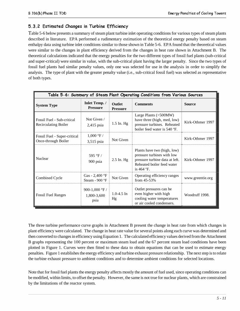
§ 316(b) Phase II TDD Energy Penalties of Cooling Towers
5 - 11
5.3.2 Estimated Changes in Turbine Efficiency
Table 5-6 below presents a summary of steam plant turbine inlet operating conditions for various types of steam plantsdescribed in literature. EPA performed a rudimentary estimation of the theoretical energy penalty based on steamenthalpy data using turbine inlet conditions similar to those shown in Table 5-6. EPA found that the theoretical valueswere similar to the changes in plant efficiency derived from the changes in heat rate shown in Attachment B. Thetheoretical calculations indicated that the energy penalties for the two different types of fossil fuel plants (sub-criticaland super-critical) were similar in value, with the sub-critical plant having the larger penalty. Since the two types offossil fuel plants had similar penalty values, only one was selected for use in the analysis in order to simplify theanalysis. The type of plant with the greater penalty value (i.e., sub-critical fossil fuel) was selected as representativeof both types.
Table 5-6: Summary of Steam Plant Operating Conditions from Various Sources
System TypeInlet Temp. /
PressureOutlet Pressure
Comments Source
Fossil Fuel - Sub-criticalRecirculating Boiler
Not Given /
2,415 psia 1.5 In. Hg
Large Plants (>500MW)have three (high, med, low)pressure turbines. Reheatedboiler feed water is 540 oF.
Kirk-Othmer 1997
Fossil Fuel - Super-criticalOnce-through Boiler
1,000 °F /
3,515 psia Not Given Kirk-Othmer 1997
Nuclear595 °F /
900 psia 2.5 In. Hg
Plants have two (high, low)pressure turbines with lowpressure turbine data at left.Reheated boiler feed wateris 464 oF.
Kirk-Othmer 1997
Combined Cycle Gas - 2,400 °FSteam - 900 °F
Not GivenOperating efficiency rangesfrom 45-53%
www.greentie.org
Fossil Fuel Ranges900-1,000 °F /
1,800-3,600psia
1.0-4.5 InHg
Outlet pressures can beeven higher with highcooling water temperaturesor air cooled condensers.
Woodruff 1998.
The three turbine performance curve graphs in Attachment B present the change in heat rate from which changes inplant efficiency were calculated. The change in heat rate value for several points along each curve was determined andthen converted to changes in efficiency using Equation 1. The calculated efficiency values derived from the AttachmentB graphs representing the 100 percent or maximum steam load and the 67 percent steam load conditions have beenplotted in Figure 1. Curves were then fitted to these data to obtain equations that can be used to estimate energypenalties. Figure 1 establishes the energy efficiency and turbine exhaust pressure relationship. The next step is to relatethe turbine exhaust pressure to ambient conditions and to determine ambient conditions for selected locations.
Note that for fossil fuel plants the energy penalty affects mostly the amount of fuel used, since operating conditions canbe modified, within limits, to offset the penalty. However, the same is not true for nuclear plants, which are constrainedby the limitations of the reactor system.
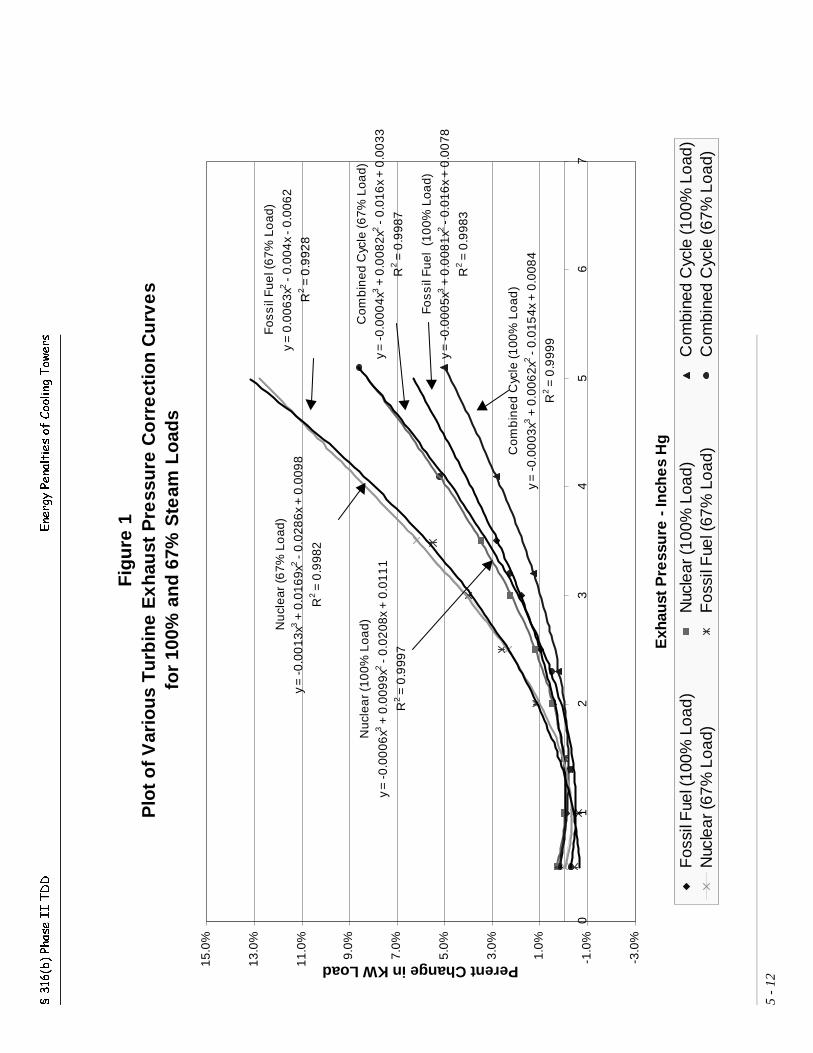
§ 3
16(b
) Ph
ase I
I T
DD
Ene
rgy
Pena
ltie
s of
Coo
ling
Tow
ers
5 -
12
Fig
ure
1P
lot
of
Var
iou
s T
urb
ine
Ex
hau
st P
ress
ure
Co
rre
ctio
n C
urv
es
for
100%
an
d 6
7% S
team
Lo
ads
Nuc
lea
r (10
0% L
oad)
y =
-0.0
006
x3 + 0
.009
9x2 -
0.02
08x
+ 0.
011
1
R2 =
0.9
997
Foss
il F
uel
(10
0% L
oad)
y =
-0.0
005x
3 + 0
.008
1x2 -
0.01
6x
+ 0
.00
78
R2 =
0.9
983
Com
bin
ed C
ycle
(100
% L
oad
)
y =
-0.0
003
x3 + 0
.006
2x2 -
0.01
54x
+ 0
.008
4
R2 =
0.9
999
Nu
clea
r (6
7% L
oad
)
y =
-0.0
013
x3 + 0
.016
9x2 -
0.02
86x
+ 0
.009
8
R2 =
0.9
982
Fos
sil
Fue
l (6
7% L
oad
)
y =
0.00
63x
2 - 0.
004
x -
0.00
62
R2 =
0.9
928
Com
bin
ed C
ycle
(67%
Loa
d)
y =
-0.0
004x
3 + 0
.008
2x2 -
0.01
6x
+ 0
.00
33
R2 =
0.9
987
-3.0
%
-1.0
%
1.0%
3.0%
5.0%
7.0%
9.0%
11.0
%
13.0
%
15.0
%
01
23
45
67
Exh
aust
Pre
ssu
re -
Inch
es
Hg
Perent Change in KW Load
Fos
sil F
uel (
100%
Loa
d)N
ucle
ar (1
00%
Loa
d)C
ombi
ned
Cyc
le (1
00%
Loa
d)N
ucle
ar (6
7% L
oad)
Fos
sil F
uel (
67%
Loa
d)C
ombi
ned
Cyc
le (6
7% L
oad)
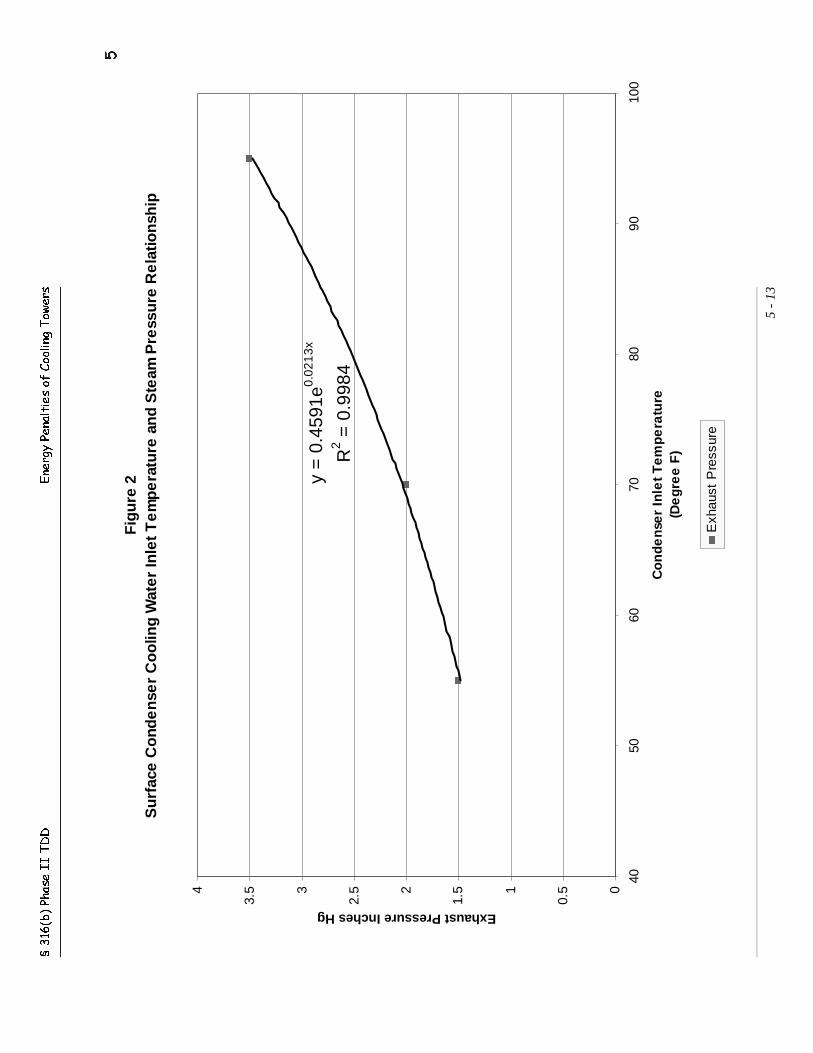
§ 3
16(b
) Ph
ase I
I T
DD
Ene
rgy
Pena
ltie
s of
Coo
ling
Tow
ers
5 -
13
Fig
ure
2S
urf
ace
Co
nde
nse
r C
oo
ling
Wat
er In
let
Te
mp
era
ture
an
d S
team
Pre
ssu
re R
ela
tion
ship
y =
0.4
591e
0.02
13x
R2 =
0.9
984
0
0.51
1.52
2.53
3.54
4050
6070
8090
100
Co
nd
en
ser
Inle
t T
em
pe
ratu
re(D
eg
ree
F)
Exhaust Pressure Inches Hg
Exh
aust
Pre
ssur
e
5
§ 316(b) Phase II TDD Energy Penalties of Cooling Towers
5 - 14
.3.3 Relationship of Condenser Cooling Water (or Air) Temperature to Steam Side Pressure
for Different Cooling System Types and Operating Conditions
˜ Surface Condensers
Both once-through and wet cooling towers use surface condensers. As noted previously, condenser inlet temperaturesof 55 °F and 95 °F will produce turbine exhaust pressures of 1.5 and 3.5 inches Hg, respectively. Additionally, datafrom the Calvert Cliffs nuclear power plant showed an exhaust pressure of 2.0 inches Hg at a cooling water temperatureof 70 °F. Figure 2 provides a plot of these data which, even though they are from two sources, appear to be consistent.A curve was fitted to these data and was used as the basis for estimating the turbine exhaust pressure for differentsurface condenser cooling water inlet temperatures. Note that this methodology is based on empirical data thatsimplifies the relationship between turbine exhaust pressure and condenser inlet temperature, which would otherwiserequire more complex heat exchange calculations. Those calculations, however, would require numerous assumptions,the selection of which may produce a different curve but with a similar general relationship.
˜ Once-through Systems
For once-through cooling systems, the steam cycle condenser cooling water inlet temperature is also the temperatureof the source water. Note that the outlet temperature of the cooling water is typically 15 - 20 °F higher than the inlettemperature. This difference is referred to as the “range.” The practical limit of the outlet temperature is approximately100 °F, since many NPDES permits have limitations in the vicinity of 102 - 105 °F . This does not appear to presenta problem, since the maximum monthly average surface water temperature at Jacksonville, Florida (selected by EPAas representing warmer U.S. surface waters) was 83.5 °F which would, using the range values above, result in aneffluent temperature of 98.5 - 103.5 °F. To gauge the turbine efficiency energy penalty for once-through coolingsystems, the temperature of the source water must be known. These temperatures will vary with location and time ofyear and estimates for several selected locations are presented in Table 5-7 below.
˜ Wet Cooling Towers
For wet cooling towers, the temperature of the cooling tower outlet is the same as the condenser cooling water inlettemperature. The performance of the cooling tower in terms of the temperature of the cooling tower outlet is a functionof the wet bulb temperature of the ambient air and the tower type, size, design, and operation. The wet bulbtemperature is a function of the ambient air temperature and the humidity. Wet bulb thermometers were historicallyused to estimate relative humidity and consist of a standard thermometer with the bulb encircled with a wet piece ofcloth. Thus, the temperature read from a wet bulb thermometer includes the cooling effect of water evaporation.
Of all of the tower design parameters, the temperature difference between the wet bulb temperature and the coolingtower outlet (referred to as the “approach”) is the most useful in estimating tower performance. The wet cooling towercooling water outlet temperature of the systems that were used in the analysis for the regulatory options had a designapproach of 10 °F. Note that the design approach value is equal to the difference between the tower cooling water outlettemperature and the ambient wet bulb temperature only at the design wet bulb temperature. The actual approach valueat wet bulb temperatures other than the design value will vary as described below.
The selection of a 10 °F design approach is based on the data in Attachment C for recently constructed towers.Moreover, a 10 °F approach is considered conservative. As can be seen in Attachment D, a plot of the tower size factorversus the approach shows that a 10 °F approach has a tower size factor of 1.5. The approach is a key factor in sizingtowers and has significant cost implications. The trade-off between selecting a small approach versus a higher valueis a trade-off between greater capital cost investment versus lower potential energy production. In states where the rates
§ 316(b) Phase II TDD Energy Penalties of Cooling Towers
5 - 15
of return on energy investments are fixed (say between 12% and 15%), the higher the capital investment, the higher thereturn.
For the wet cooling towers used in this analysis, the steam cycle condenser inlet temperature is set equal to the ambientair wet bulb temperature for the location plus the estimated approach value. A design approach value of 10 °F wasselected as the common design value for all locations. However, this value is only applicable to instances when theambient wet bulb temperature is equal to the design wet bulb temperature. In this analysis, the design wet bulbtemperature was selected as the 1 percent exceedence value for the specific selected locations.
Attachment E provides a graph showing the relationship between different ambient wet bulb temperatures and thecorresponding approach for a “typical” wet tower. The graph shows that as the ambient wet bulb temperaturedecreases, the approach value increases. The graph in Attachment E was used as the basis for estimating the changein the approach value as the ambient wet bulb temperature changes from the design value for each location. Differencesin the location-specific design wet bulb temperature were incorporated by fitting a second order polynomial equationto the data in this graph. The equation was then modified by adjusting the intercept value such that the approach wasequal to 10 °F when the wet bulb temperature was equal to the design 1 percent wet bulb temperature for the selectedlocation. The location-specific equations were then used to estimate the condenser inlet temperatures that correspondto the estimated monthly values for wet bulb temperatures at the selected locations.
˜ Air Cooled Condensers
Air cooled condensers reject heat by conducting it directly from the condensing steam to the ambient air by forcing theair over the heat conducting surface. No evaporation of water is involved. Thus, for air cooled condensers, thecondenser performance with regard to turbine exhaust pressure is directly related to the ambient (dry bulb) airtemperature, as well as to the condenser design and operating conditions. Note that dry bulb temperature is the sameas the standard ambient air temperature with which most people are familiar. Figure 3 presents a plot of the designambient air temperature and corresponding turbine exhaust pressure for air cooled condensers recently installed by amajor cooling system manufacturer (GEA Power Cooling Systems, Inc.). An analysis of the multiple facility data inFigure 3 did not find any trends with respect to plant capacity, location, or age that could justify the separation of thesedata into subgroups. Three facilities that had very large differences (i.e., >80 oF) in the design dry bulb temperaturecompared to the temperature of saturated steam at the exhaust pressure were deleted from the data set used in Figure3.
A review of the design temperatures indicated that the design temperatures did not always correspond to annualtemperature extremes of the location of the plant as might be expected. Thus, it appears that the selection of designvalues for each application included economic considerations. EPA concluded that these design data represent therange of condenser performance at different temperatures and design conditions. A curve was fitted to the entire setof data to serve as a reasonable means of estimating the relationship of turbine exhaust pressure to different ambientair (dry bulb) temperatures. To validate this approach, condenser performance data for a power plant from anengineering contractor report (Litton, no date) was also plotted. This single plant data produced a flatter curve thanthe multi-facility plot. In other words, the multi-facility curve predicts a greater increase in turbine exhaust pressureas the dry bulb temperature increases. Therefore, the multi-facility curve was selected as a conservative estimation ofthe relationship between ambient air temperatures and the turbine exhaust pressure. Note that in the case of air cooledcondensers, the turbine exhaust steam pressure includes values above 3.5 inches Hg.
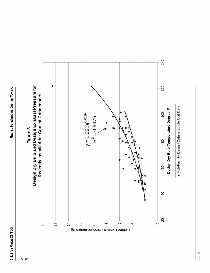
§ 3
16(b
) Ph
ase I
I T
DD
Ene
rgy
Pena
ltie
s of
Coo
ling
Tow
ers
5 -
16
Fig
ure
3D
esig
n D
ry B
ulb
an
d D
esig
n E
xhau
st P
ress
ure
for
Rec
ently
Inst
alle
d A
ir C
oo
led
Co
nd
ense
rs
y =
1.0
31e
0.01
9x
R2 =
0.6
976
024681012141618
2040
6080
100
120
140
De
sig
n D
ry B
ulb
Te
mp
era
ture
De
gre
e F
Turbine Exhaust Pressure Inches Hg
Mul
i-Fac
ility
Des
ign
Dat
aS
ingl
e U
nit
Dat
a
˜ R
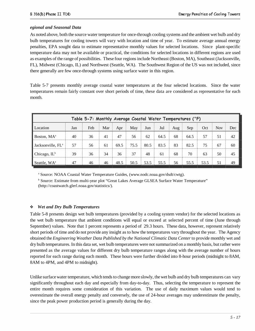
§ 316(b) Phase II TDD Energy Penalties of Cooling Towers
5 - 17
egional and Seasonal Data
As noted above, both the source water temperature for once-through cooling systems and the ambient wet bulb and drybulb temperatures for cooling towers will vary with location and time of year. To estimate average annual energypenalties, EPA sought data to estimate representative monthly values for selected locations. Since plant-specifictemperature data may not be available or practical, the conditions for selected locations in different regions are usedas examples of the range of possibilities. These four regions include Northeast (Boston, MA), Southeast (Jacksonville,FL), Midwest (Chicago, IL) and Northwest (Seattle, WA). The Southwest Region of the US was not included, sincethere generally are few once-through systems using surface water in this region.
Table 5-7 presents monthly average coastal water temperatures at the four selected locations. Since the watertemperatures remain fairly constant over short periods of time, these data are considered as representative for eachmonth.
Table 5-7: Monthly Average Coastal Water Temperatures (°F)
Location Jan Feb Mar Apr May Jun Jul Aug Sep Oct Nov Dec
Boston, MAa 40 36 41 47 56 62 64.5 68 64.5 57 51 42
Jacksonville, FLa 57 56 61 69.5 75.5 80.5 83.5 83 82.5 75 67 60
Chicago, ILb 39 36 34 36 37 48 61 68 70 63 50 45
Seattle, WAa 47 46 46 48.5 50.5 53.5 55.5 56 55.5 53.5 51 49
a Source: NOAA Coastal Water Temperature Guides, (www.nodc.noaa.gov/dsdt/cwtg).b Source: Estimate from multi-year plot “Great Lakes Average GLSEA Surface Water Temperature” (http://coastwatch.glerl.noaa.gov/statistics/).
˜ Wet and Dry Bulb Temperatures
Table 5-8 presents design wet bulb temperatures (provided by a cooling system vendor) for the selected locations asthe wet bulb temperature that ambient conditions will equal or exceed at selected percent of time (June throughSeptember) values. Note that 1 percent represents a period of 29.3 hours. These data, however, represent relativelyshort periods of time and do not provide any insight as to how the temperatures vary throughout the year. The Agencyobtained the Engineering Weather Data Published by the National Climatic Data Center to provide monthly wet anddry bulb temperatures. In this data set, wet bulb temperatures were not summarized on a monthly basis, but rather werepresented as the average values for different dry bulb temperature ranges along with the average number of hoursreported for each range during each month. These hours were further divided into 8-hour periods (midnight to 8AM,8AM to 4PM, and 4PM to midnight).
Unlike surface water temperature, which tends to change more slowly, the wet bulb and dry bulb temperatures can varysignificantly throughout each day and especially from day-to-day. Thus, selecting the temperature to represent theentire month requires some consideration of this variation. The use of daily maximum values would tend tooverestimate the overall energy penalty and conversely, the use of 24-hour averages may underestimate the penalty,since the peak power production period is generally during the day.
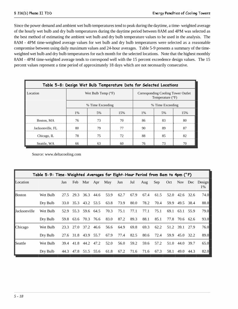
§ 316(b) Phase II TDD Energy Penalties of Cooling Towers
5 - 18
Since the power demand and ambient wet bulb temperatures tend to peak during the daytime, a time- weighted averageof the hourly wet bulb and dry bulb temperatures during the daytime period between 8AM and 4PM was selected asthe best method of estimating the ambient wet bulb and dry bulb temperature values to be used in the analysis. The8AM - 4PM time-weighted average values for wet bulb and dry bulb temperatures were selected as a reasonablecompromise between using daily maximum values and 24-hour averages. Table 5-9 presents a summary of the time-weighted wet bulb and dry bulb temperatures for each month for the selected locations. Note that the highest monthly8AM - 4PM time-weighted average tends to correspond well with the 15 percent exceedence design values. The 15percent values represent a time period of approximately 18 days which are not necessarily consecutive.
Table 5-8: Design Wet Bulb Temperature Data for Selected Locations
Location Wet Bulb Temp (°F) Corresponding Cooling Tower Outlet Temperature (°F)
% Time Exceeding % Time Exceeding
1% 5% 15% 1% 5% 15%
Boston, MA 76 73 70 86 83 80
Jacksonville, FL 80 79 77 90 89 87
Chicago, IL 78 75 72 88 85 82
Seattle, WA 66 63 60 76 73 70
Source: www.deltacooling.com
Table 5-9: Time-Weighted Averages for Eight-Hour Period from 8am to 4pm (°F)
Location Jan Feb Mar Apr May Jun Jul Aug Sep Oct Nov Dec Design1%
Boston Wet Bulb 27.5 29.3 36.3 44.6 53.9 62.7 67.9 67.4 61.5 52.0 42.6 32.6 74.0
Dry Bulb 33.0 35.3 43.2 53.5 63.8 73.9 80.0 78.2 70.4 59.9 49.5 38.4 88.0
Jacksonville Wet Bulb 52.9 55.3 59.6 64.5 70.3 75.1 77.1 77.1 75.1 69.1 63.1 55.9 79.0
Dry Bulb 59.8 63.6 70.3 76.6 83.0 87.2 89.3 88.1 85.1 77.8 70.6 62.6 93.0
Chicago Wet Bulb 23.3 27.0 37.2 46.6 56.6 64.9 69.8 69.3 62.2 51.2 39.1 27.9 76.0
Dry Bulb 27.6 31.8 43.9 55.7 67.9 77.4 82.5 80.6 72.4 59.9 45.0 32.2 89.0
Seattle Wet Bulb 39.4 41.8 44.2 47.2 52.0 56.0 59.2 59.6 57.2 51.0 44.0 39.7 65.0
Dry Bulb 44.3 47.8 51.5 55.6 61.8 67.2 71.6 71.6 67.3 58.1 49.0 44.3 82.0

§ 316(b) Phase II TDD Energy Penalties of Cooling Towers
5 - 19
5.3.4 Calculation of Energy Penalty
Since the energy penalty will vary over time as ambient climatic and source water temperatures vary, the calculationof the total annual energy penalty for a chosen location would best be performed by combining (integrating) the resultsof individual calculations performed on a periodic basis. For this analysis, a monthly basis was chosen.
The estimated monthly turbine exhaust pressure values for alternative cooling system scenarios were derived using thecurves in Figures 2 and 3 in conjunction with the monthly temperature values in Tables 5-7 and 5-9. These turbineexhaust pressure values were then used to estimate the associated change in turbine efficiency using the equations fromFigure 1. EPA then calculated the energy penalty for each month. Annual values were calculated by averaging the 12monthly values.
Tables 5-10 and 5-11 present a summary of the calculated annual average energy penalty values for steam rates of 100percent and 67 percent of maximum load. These values can be applied directly to the power plant output to determineeconomic and other impacts. In other words, an energy penalty of 2 percent indicates that the plant output power wouldbe reduced by 2 percent. In addition, Tables 5-10 and 5-11 include the maximum turbine energy penalty associatedwith maximum design conditions such as once-through systems drawing water at the highest monthly average, and wettowers and air cooled condensers operating in air with a wet bulb and dry bulb temperature at the 1 percent exceedencelevel. EPA notes that the maximum design values result from using the maximum monthly water temperatures fromTable 5-7 and the 1% percent exceedence wet bulb and dry bulb temperatures from Table 5-8.
EPA notes that the penalties presented in Tables 5-10 and 5-11 do not comprise the total energy penalties (whichincorporate all three components of energy penalties: turbine efficiency penalty, fan energy requirements, and pumpingenergy usage) as a percent of power output. The total energy penalties are presented in section 5.1 above. The tablesbelow only present the turbine efficiency penalty. Section 5.4 presents the fan and pumping components of the energypenalty.
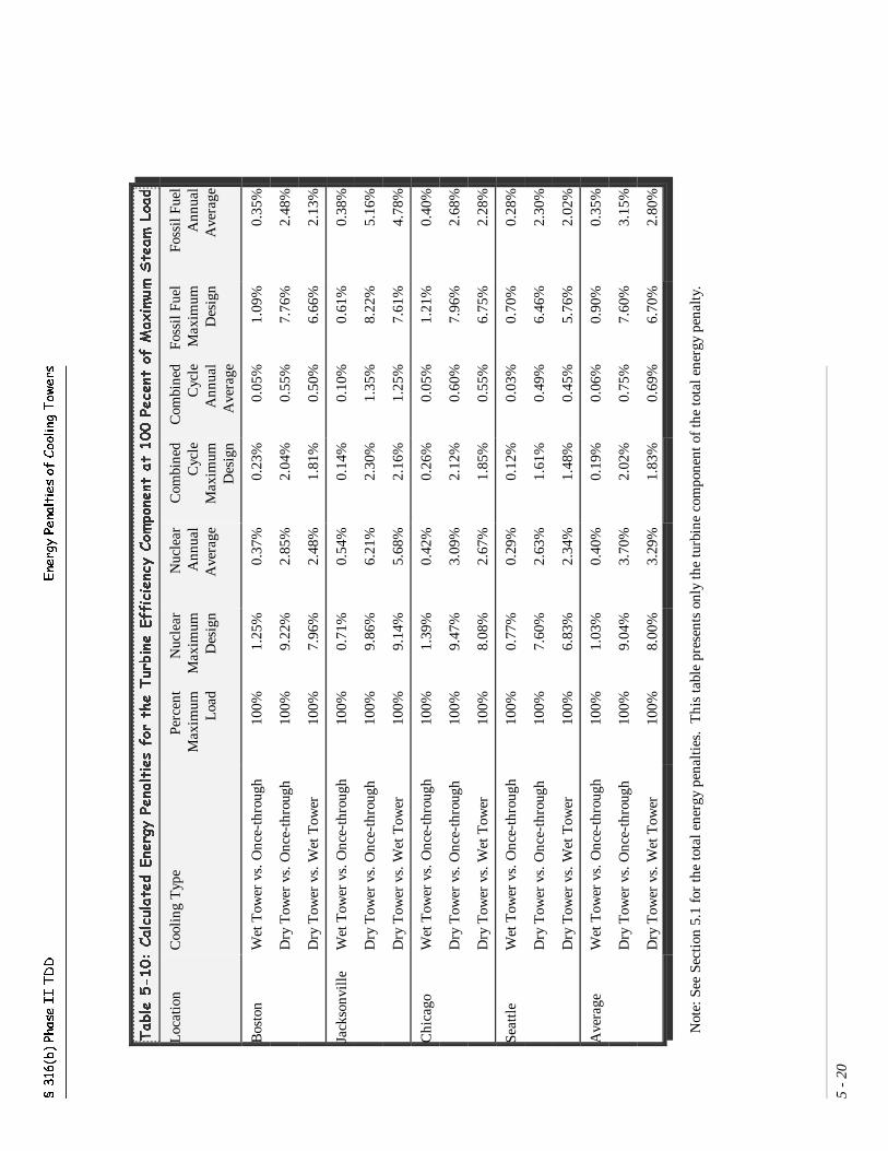
§ 3
16(b
) Ph
ase I
I T
DD
Ene
rgy
Pena
ltie
s of
Coo
ling
Tow
ers
5 -
20
Table 5
-10:
Calculate
d E
nerg
y P
ena
lties
for
the T
urbine E
fficienc
y C
ompo
nent
at
100 P
ece
nt o
f M
axim
um S
team L
oad
Loc
atio
nC
ooli
ng T
ype
Perc
ent
Max
imum
Loa
d
Nuc
lear
Max
imum
Des
ign
Nuc
lear
Ann
ual
Ave
rage
Com
bine
dC
ycle
Max
imum
Des
ign
Com
bine
dC
ycle
Ann
ual
Ave
rage
Foss
il F
uel
Max
imum
Des
ign
Foss
il F
uel
Ann
ual
Ave
rage
Bos
ton
Wet
Tow
er v
s. O
nce-
thro
ugh
100%
1.25
%0.
37%
0.23
%0.
05%
1.09
%0.
35%
Dry
Tow
er v
s. O
nce-
thro
ugh
100%
9.22
%2.
85%
2.04
%0.
55%
7.76
%2.
48%
Dry
Tow
er v
s. W
et T
ower
100%
7.96
%2.
48%
1.81
%0.
50%
6.66
%2.
13%
Jack
sonv
ille
Wet
Tow
er v
s. O
nce-
thro
ugh
100%
0.71
%0.
54%
0.14
%0.
10%
0.61
%0.
38%
Dry
Tow
er v
s. O
nce-
thro
ugh
100%
9.86
%6.
21%
2.30
%1.
35%
8.22
%5.
16%
Dry
Tow
er v
s. W
et T
ower
100%
9.14
%5.
68%
2.16
%1.
25%
7.61
%4.
78%
Chi
cago
Wet
Tow
er v
s. O
nce-
thro
ugh
100%
1.39
%0.
42%
0.26
%0.
05%
1.21
%0.
40%
Dry
Tow
er v
s. O
nce-
thro
ugh
100%
9.47
%3.
09%
2.12
%0.
60%
7.96
%2.
68%
Dry
Tow
er v
s. W
et T
ower
100%
8.08
%2.
67%
1.85
%0.
55%
6.75
%2.
28%
Seat
tle
Wet
Tow
er v
s. O
nce-
thro
ugh
100%
0.77
%0.
29%
0.12
%0.
03%
0.70
%0.
28%
Dry
Tow
er v
s. O
nce-
thro
ugh
100%
7.60
%2.
63%
1.61
%0.
49%
6.46
%2.
30%
Dry
Tow
er v
s. W
et T
ower
100%
6.83
%2.
34%
1.48
%0.
45%
5.76
%2.
02%
Ave
rage
Wet
Tow
er v
s. O
nce-
thro
ugh
100%
1.03
%0.
40%
0.19
%0.
06%
0.90
%0.
35%
Dry
Tow
er v
s. O
nce-
thro
ugh
100%
9.04
%3.
70%
2.02
%0.
75%
7.60
%3.
15%
Dry
Tow
er v
s. W
et T
ower
100%
8.00
%3.
29%
1.83
%0.
69%
6.70
%2.
80%
Not
e: S
ee S
ecti
on 5
.1 f
or th
e to
tal e
nerg
y pe
nalt
ies.
Thi
s ta
ble
pres
ents
onl
y th
e tu
rbin
e co
mpo
nent
of
the
tota
l ene
rgy
pena
lty.
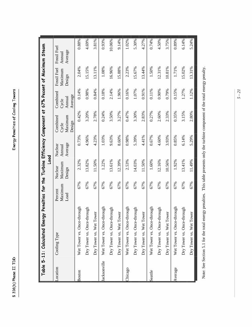
§ 3
16(b
) Ph
ase I
I T
DD
Ene
rgy
Pena
ltie
s of
Coo
ling
Tow
ers
5 -
21
Table 5
-11:
Calculate
d E
nerg
y P
ena
lties
for
the T
urbine E
fficienc
y C
ompo
nent
at
67% P
ece
nt o
f M
axim
um S
team
Loa
d
Loc
atio
nC
ooli
ng T
ype
Perc
ent
Max
imum
Loa
d
Nuc
lear
Max
imum
Des
ign
Nuc
lear
Ann
ual
Ave
rage
Com
bine
dC
ycle
Max
imum
Des
ign
Com
bine
dC
ycle
Ann
ual
Ave
rage
Foss
il F
uel
Max
imum
Des
ign
Foss
il F
uel
Ann
ual
Ave
rage
Bos
ton
Wet
Tow
er v
s. O
nce-
thro
ugh
67%
2.32
%0.
73%
0.42
%0.
14%
2.04
%0.
88%
Dry
Tow
er v
s. O
nce-
thro
ugh
67%
13.8
2%4.
96%
3.20
%0.
98%
15.1
5%4.
69%
Dry
Tow
er v
s. W
et T
ower
67%
11.5
0%4.
23%
2.78
%0.
84%
13.1
1%3.
81%
Jack
sonv
ille
Wet
Tow
er v
s. O
nce-
thro
ugh
67%
1.22
%1.
03%
0.24
%0.
18%
1.08
%0.
93%
Dry
Tow
er v
s. O
nce-
thro
ugh
67%
13.6
1%9.
63%
3.50
%2.
14%
16.9
6%10
.06%
Dry
Tow
er v
s. W
et T
ower
67%
12.3
9%8.
60%
3.27
%1.
96%
15.8
8%9.
14%
Chi
cago
Wet
Tow
er v
s. O
nce-
thro
ugh
67%
2.53
%0.
98%
0.47
%0.
16%
2.23
%1.
02%
Dry
Tow
er v
s. O
nce-
thro
ugh
67%
14.0
3%5.
39%
3.30
%1.
07%
15.6
7%5.
30%
Dry
Tow
er v
s. W
et T
ower
67%
11.5
0%4.
41%
2.83
%0.
91%
13.4
4%4.
27%
Seat
tle
Wet
Tow
er v
s. O
nce-
thro
ugh
67%
1.60
%0.
67%
0.27
%0.
11%
1.50
%0.
74%
Dry
Tow
er v
s. O
nce-
thro
ugh
67%
12.1
6%4.
60%
2.60
%0.
90%
12.3
1%4.
50%
Dry
Tow
er v
s. W
et T
ower
67%
10.5
6%3.
93%
2.33
%0.
79%
10.8
1%3.
75%
Ave
rage
Wet
Tow
er v
s. O
nce-
thro
ugh
67%
1.92
%0.
85%
0.35
%0.
15%
1.71
%0.
89%
Dry
Tow
er v
s. O
nce-
thro
ugh
67%
13.4
1%6.
14%
3.15
%1.
27%
15.0
2%6.
14%
Dry
Tow
er v
s. W
et T
ower
67%
11.4
9%5.
29%
2.80
%1.
12%
13.3
1%5.
24%
Not
e: S
ee S
ecti
on 5
.1 f
or th
e to
tal e
nerg
y pe
nalt
ies.
Thi
s ta
ble
pres
ents
onl
y th
e tu
rbin
e co
mpo
nent
of
the
tota
l ene
rgy
pena
lty.
§ 316(b) Phase II TDD Energy Penalties of Cooling Towers
5 - 22
5.4 ENERGY PENALTY ASSOCIATED WITH COOLING SYSTEM ENERGY REQUIREMENTS
This analysis is presented to evaluate the energy requirements associated with the operation of the alternative types ofcooling systems. As noted previously, the reductions in energy output resulting from the energy required to operate thecooling system equipment are often referred to as parasitic losses. In evaluating this component of the energy penalty,it is the differences between the parasitic losses of the alternative systems that are important. In general, the costsassociated with the cooling system energy requirements have been included within the annual O&M cost values forcertain regulatory options developed using the methodologies presented in Chapter 2 of this document. Thus, the costsof the cooling system operating energy requirements do not need to be factored into the overall energy penalty costanalysis as a separate value.
Alternative cooling systems can create additional energy demands primarily through the use of fans and pumps. Thereare other energy demands such as treatment of tower blowdown, but these are insignificant compared to the pump andfan requirements and will not be included here. Some seasonal variation may be expected due to reduced requirementsfor cooling media flow volume during colder periods. These reduced requirements can include reduced cooling waterpumping for once-through systems and reduced fan energy requirements for both wet and dry towers. However, noadjustments were made concerning the potential seasonal variations in cooling water pumping. The seasonal variationin fan power requirements is accounted for in this evaluation by applying an annual fan usage rate. The pumpingenergy estimates are calculated using a selected cooling water flow rate of 100,000 gpm (223 cfs).
5.4.1 Fan Power Requirements
˜ Wet Towers
In the reference Cooling Tower Technology (Burger 1995), several examples are provided for cooling towers with flowrates of 20,000 gpm using 4 cells with either 75 (example #1) or 100 Hp (example #2) fans each. The primarydifference between these two examples is that the tower with the higher fan power requirement has an approach of 5oF compared to 11 oF for the tower with the lower fan power requirement. Using an electric motor efficiency of 92percent and a fan usage factor of 93 percent (Fleming 2001), the resulting fan electric power requirements are equalto 0.236 MW and 0.314 MW for the four cells with 75 and 100 Hp fan motors, respectively. These example towersboth had a heat load of 150 million BTU/hr. Table 5-14 provides the percent of power output penalty based onequivalent plant capacities derived using the heat rejection factors described below. Note that fan gear efficiency valuesare not applicable because they do not affect the fan motor power rating or the amount of electricity required to operatethe fan motors.
A third example was provided in vendor-supplied data (Fleming 2001), in which a cooling tower with a cooling waterflow rate of 243,000 gpm had a total fan motor capacity brake-Hp of 250 for each of 12 cells. This wet tower had adesign temperature range of 15 °F and an approach of 10 °F. The percent of power output turbine penalty shown inTables 5-10 and 5-11 is also based on equivalent plant capacities derived using the heat rejection factors describedbelow.
A fourth example is a cross-flow cooling tower for a 35 MW coal-fired plant in Iowa (Litton, no date). In this example,the wet tower consists of two cells with one 150 Hp fan each, with a cooling water flow rate of 30,000 gpm. This wettower had a design temperature range of 16 °F, an approach of 12 °F, and wet bulb temperature of 78 °F. Thecalculated energy penalty in this example is 0.67 percent.
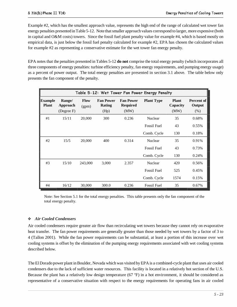
§ 316(b) Phase II TDD Energy Penalties of Cooling Towers
5 - 23
Example #2, which has the smallest approach value, represents the high end of the range of calculated wet tower fanenergy penalties presented in Table 5-12. Note that smaller approach values correspond to larger, more expensive (bothin capital and O&M costs) towers. Since the fossil fuel plant penalty value for example #4, which is based mostly onempirical data, is just below the fossil fuel penalty calculated for example #2, EPA has chosen the calculated valuesfor example #2 as representing a conservative estimate for the wet tower fan energy penalty.
EPA notes that the penalties presented in Tables 5-12 do not comprise the total energy penalty (which incorporates allthree components of energy penalties: turbine efficiency penalty, fan energy requirements, and pumping energy usage)as a percent of power output. The total energy penalties are presented in section 3.1 above. The table below onlypresents the fan component of the penalty.
Table 5-12: Wet Tower Fan Power Energy Penalty
ExamplePlant
Range/Approach
(Degree F)
Flow
(gpm)
Fan PowerRating
(Hp)
Fan PowerRequired
(MW)
Plant Type PlantCapacity
(MW)
Percent ofOutput
(%)
#1 15/11 20,000 300 0.236 Nuclear 35 0.68%
Fossil Fuel 43 0.55%
Comb. Cycle 130 0.18%
#2 15/5 20,000 400 0.314 Nuclear 35 0.91%
Fossil Fuel 43 0.73%
Comb. Cycle 130 0.24%
#3 15/10 243,000 3,000 2.357 Nuclear 420 0.56%
Fossil Fuel 525 0.45%
Comb. Cycle 1574 0.15%
#4 16/12 30,000 300.0 0.236 Fossil Fuel 35 0.67%
Note: See Section 5.1 for the total energy penalties. This table presents only the fan component of thetotal energy penalty.
˜ Air Cooled Condensers
Air cooled condensers require greater air flow than recirculating wet towers because they cannot rely on evaporativeheat transfer. The fan power requirements are generally greater than those needed by wet towers by a factor of 3 to4 (Tallon 2001). While the fan power requirements can be substantial, at least a portion of this increase over wetcooling systems is offset by the elimination of the pumping energy requirements associated with wet cooling systemsdescribed below.
The El Dorado power plant in Boulder, Nevada which was visited by EPA is a combined-cycle plant that uses air cooledcondensers due to the lack of sufficient water resources. This facility is located in a relatively hot section of the U.S.Because the plant has a relatively low design temperature (67 oF) in a hot environment, it should be considered asrepresentative of a conservative situation with respect to the energy requirements for operating fans in air cooled
§ 316(b) Phase II TDD Energy Penalties of Cooling Towers
5 - 24
condensers. The steam portion of the plant has a capacity of 150 MW (1.1 million lb/hr steam flow). The air cooledcondensers consist of 30 cells with a 200 Hp fan each. A fan motor efficiency of 92 percent is assumed. Each fan hastwo operating speeds, with the low speed consuming 20 percent of the fan motor power rating.
The facility manager provided estimates of the proportion of time that the fans were operated at low or full speed duringdifferent portions of the year (Tatar 2001). Factoring in the time proportions and the corresponding power requirementsresults in an overall annual fan power factor of 72 percent for this facility. In other words, over a one year period, thefan power requirement will average 75 percent of the fan motor power rating. A comparison of the climatic data forLas Vegas (located nearby) and Jacksonville, Florida shows that the Jacksonville mean maximum temperature valueswere slightly warmer in the winter and slightly cooler in the summer. Adjustments in the annual fan power factorcalculations to address Jacksonville’s slightly warmer winter months resulted in a projected annual fan power factorof 77 percent. EPA chose a factor of 75 percent as representative of warmer regions of the U.S. Due to lack ofavailable operational data for other locations, this value is used for facilities throughout the U.S. and represents anconservative value for the much cooler regions.
Prior to applying this factor, the resulting maximum energy penalty during warmer months is 3.2 percent for the steamportion only. This value is the maximum instantaneous penalty that would be experienced during high temperatureconditions. When the annual fan power factor of 75 percent is applied, the annual fan energy penalty becomes 2.4percent of the plant power output. An engineer from an air cooled condenser manufacturer indicated that the majorityof air cooled condensers being installed today also include two-speed fans and that the 20 percent power ratio for thelow speed was the factor that they used also. In fact, some dry cooling systems, particularly those in very cold regions,use fans with variable speed drives to provide even better operational control. Similar calculations for a waste-to-energy plant in Spokane, Washington resulted in a maximum fan operating penalty of 2.8 percent and an annual averageof 2.1 percent using the 75 percent fan power factor. Thus, the factor of 2.4 percent selected by EPA as a conservativeannual penalty value appears valid.
5.4.2 Cooling Water Pumping Requirements
The Agency notes that it conducted the following analysis for new, “greenfield” facilities and transferred the results ofthis analysis to the cooling system conversions for existing facilities considered as regulatory options for this proposal.As discussed in Section 5.6 below, the Department of Energy (DOE) concludes in their draft energy penalty analysisthat the pumping component of the energy penalty for existing facilities may be higher than calculated herein by EPAfor new, “greenfield” facilities.
The energy requirements for cooling water pumping can be estimated by combining the flow rates and the total head(usually given in feet of water) that must be pumped. Estimating the power requirements for the alternative coolingsystems that use water is somewhat complex in that there are several components to the total pumping head involved.For example, a once-through system must pump water from the water source to the steam condensers, which willinclude both a static head from the elevation of the source to the condenser (use of groundwater would represent anextreme case) and friction head losses through the piping and the condenser. The pipe friction head is dependent on thedistance between the power plant and the source plus the size and number of pipes, pipe fittings, and the flow rate. Thecondenser friction head loss is a function of the condenser design and flow rate.
§ 316(b) Phase II TDD Energy Penalties of Cooling Towers
5 - 25
Wet cooling towers must also pump water against both a static and friction head. A power plant engineering consultantestimated that the total pumping head at a typical once-through facility would be approximately 50 ft (Taylor 2001).EPA performed a detailed analysis of the cooling water pumping head that would result from different combinationsof piping velocities and distances. The results of this analysis showed that the pumping head was in many scenariossimilar in value for both once-through and wet towers, and that the estimated pumping head ranged from approximately40 to 60 feet depending on the assumed values. Since EPA’s analysis produced similar values as the 50 ft pumpinghead provided by the engineering consultant, this value was used in the estimation of the pumping requirements forcooling water intakes for both once-through and wet tower systems. The following sections describe the method forderiving these pumping head values.
˜ Friction Losses
In order to provide a point of comparison, a cooling water flow rate of 100,000 gpm (223 cfs) was used. A recentlyreported general pipe sizing rule indicating that a pipe flow velocity of 5.7 fps is the optimum flow rate with regardsto the competing cost values was used as the starting point for flow velocity (Durand et al. 1999). Such a minimumvelocity is needed to prevent sediment deposition and pipe fouling. Using this criterion as a starting point, four 42-inchsteel pipes carrying 25,000 gpm each at a velocity of 5.8 fps were selected. Each pipe would have a friction head lossof 0.358 ft/100 ft of pipe (Permutit 1961), resulting in a friction loss of 3.6 ft for every 1,000 ft of length. Since capitalcosts may dictate using fewer pipes with greater pipe flow rates, two other scenarios using either three or two parallel42-inch pipes were also evaluated. Three pipes would result in a flow rate and velocity of 33,000 gpm and 7.7 fps,which results in a friction head loss of 6.1 ft/1000ft. Two pipes would result in a flow rate and velocity of 50,000 gpmand 11.6 fps, which results in a friction head loss of 12.8 ft/1000ft. The estimated 50 ft total pumping head was mostconsistent with a pipe velocity of 7.7 fps (three 42-inch pipes).
The relative distances of the power plant condensers to the once-through cooling water intakes as compared to thedistance from the plant to the alternative cooling tower can be an important factor. In general, the distances that thelarge volumes of cooling water must be pumped will be greater for once-through cooling systems. For this analysis, afixed distance of 300 ft was selected for the cooling tower. Various distances ranging from 300 ft to 3,000 ft are usedfor the once-through system. The friction head was also assumed to include miscellaneous losses due to inlets, outlets,bends, valves, etc., which can be calculated using equivalent lengths of pipe. For 42-in. steel pipe, each entrance andlong sweep elbow is equal to about 60 ft in added pipe length. For the purposes of this analysis, both systems wereassumed to have five such fittings for an added length of 300 ft. The engineering estimate of 50 ft for pumping headwas most consistent with a once-through pumping distance of approximately 1,000 ft.
˜ Static Head
Static head refers to the distance in height that the water must be pumped from the source elevation to the destination.In the case of once-through cooling systems, this is the distance in elevation between the source water and the condenserinlet. However, many power plants eliminate a significant portion of the static head loss by operating the condenserpiping as a siphon. This is done by installing vacuum pumps at the high point of the water loop. In EPA’s analysis,a static head of 20 ft produced a total pumping head value that was most consistent with the engineering consultant’sestimate of 50 feet.
In the case of cooling towers, static head is related to the height of the tower, and vendor data for the overall pumpinghead through the tower is available. This pumping head includes both the static and dynamic heads within the tower,
§ 316(b) Phase II TDD Energy Penalties of Cooling Towers
5 - 26
but was included as the static head component for the analysis. Vendor data reported a total pumping head of 25 ft fora large cooling tower sized to handle 335,000 gpm (Fleming 2001). The tower is a counter-flow packed tower design.Adding the condenser losses and pipe losses resulted in a total pumping head of approximately 50 feet.
˜ Condenser Losses
Condenser design data provided by a condenser manufacturer, Graham Corporation, showed condenser head lossesranging from 21 ft of water for small condensers (cooling flow <50,000 gpm) to 41 ft for larger condensers (Hess2001). Another source showed head losses through the tubes of a large condenser (311,000 gpm) to be approximately9 ft of water (HES. 2001). For the purposes of this analysis, EPA estimated condenser head losses to be 20 ft of water.For comparable systems with similar cooling water flow rates, the condenser head loss component should be the samefor both once-through systems and recirculating wet towers.
˜ Flow Rates
In general, the cooling water flow rate is a function of the heat rejection rate through the condensers and the range oftemperature between the condenser inlet and outlet. The flow rate for cooling towers is approximately 95 percent thatof once-through cooling water systems, depending on the cooling temperature range. However, cooling tower systemsalso still require some pumping of make-up water. For the purposes of this analysis, the flow rates for each system willbe assumed to be essentially the same. All values used in the calculations are for a cooling water flow rate of 100,000gpm. Values for larger and smaller systems can be factored against these values. The total pump and motor efficiencyis assumed to be equal to 70 percent.
5.5 ANALYSIS OF COOLING SYSTEM ENERGY REQUIREMENTS
This analysis evaluates the energy penalty associated with the operation of cooling system equipment for conversionfrom once-through systems to wet towers and for conversion to air cooled systems by estimating the net difference inrequired pumping and fan energy between the systems. This penalty can then be compared to the power outputassociated with a cooling flow rate of 100,000 gpm to derive a percent of plant output figure that is a similar measureto the turbine efficiency penalty described earlier. The power output was determined by comparing condenser heatrejection rates for different types of systems. As noted earlier, the cost of this energy penalty component has alreadybeen included in the alternative cooling system O&M costs discussed in Chapter 2 of this document, but was derivedindependently for this analysis.
Table 5-13 shows the pumping head and energy requirements for pumping 100,000 gpm of cooling water for both once-through and recirculating wet towers using the various piping scenario assumptions. In general, the comparison of twotypes of cooling systems shows offsetting energy requirements that essentially show zero pumping penalty betweenonce-through and wet towers as the pumping distance for the once-through system increases to approximately 1,000ft. In fact, it is apparent that for once-through systems with higher pipe velocities and pumping distances, more coolingwater pumping energy may be required for the once-through system than for a wet cooling tower. Thus, whenconverting from once-through to recirculating wet towers, the differences in pumping energy requirements may berelatively small.
As described above, wet towers will require additional energy to operate the fans, which results in a net increase in theenergy needed to operate the wet tower cooling system compared to once-through. Note that the average calculated

§ 316(b) Phase II TDD Energy Penalties of Cooling Towers
5 - 27
pumping head across the various scenarios for once-through systems was 54 ft. This data suggests that an averagepumping head of 50 feet for once-through systems appears to be a reasonable assumption where specific data are notavailable.
EPA notes that the penalties presented in Tables 5-13 and 5-14 do not comprise the total energy penalties (whichincorporate all three components of energy penalties: turbine efficiency penalty, fan energy requirements, and pumpingenergy usage) as a percent of power output. The total energy penalties are presented in section 3.1 above. The tablesbelow only present the pumping components.
§ 3
16(b
) Ph
ase I
I T
DD
Ene
rgy
Pena
ltie
s of
Coo
ling
Tow
ers
5 -
28Table 5
-13:
Cooling W
ate
r Pumping H
ead a
nd E
nerg
y f
or
100,0
00 g
pm S
yst
em W
et
Towers
Vers
us
Once-th
rough A
t 20'
Sta
tic H
ead
Coo
ling
Syst
em T
ype
Dis
tanc
e
Pum
ped
Stat
ic
Hea
d
Con
dens
er
Hea
d
Equ
iv.
Len
gth
Mis
c.L
osse
s
Pipe
Vel
ocit
y
Fric
tion
Los
sR
ate
Fric
tion
Hea
d
Tot
al
Hea
d
Net
Dif
fere
nce
Flow
Rat
eH
ydra
ulic
-H
pB
rake
-H
pPo
wer
Req
uire
d
Ene
rgy
Pena
lty
ft.
ft.
ftft
.fp
sft
/1,0
00ft
ft.
ft.
ftgp
mH
pH
pkW
kWO
nce-
thro
ugh
at 2
0' S
tati
c H
ead
Usi
ng 4
: 42
" P
ipes
at
300'
Len
gth
Onc
e-th
roug
h30
020
2130
05.
83.
62
4310
0,00
010
8915
5611
61W
et T
ower
300
2521
300
5.8
3.6
248
510
0,00
012
1617
3712
9613
5O
nce-
thro
ugh
at 2
0' S
tati
c H
ead
Usi
ng 3
: 42
" P
ipes
at
300'
Len
gth
Onc
e-th
roug
h30
020
2130
07.
76.
14
4510
0,00
011
2716
1012
01W
et T
ower
300
2521
300
7.7
6.1
450
510
0,00
012
5417
9113
3613
5O
nce-
thro
ugh
at 2
0' S
tati
c H
ead
Usi
ng 2
: 42
" P
ipes
at
300'
Len
gth
Onc
e-th
roug
h30
020
2130
011
.612
.88
4910
0,00
012
2917
5513
10W
et T
ower
300
2521
300
11.6
12.8
854
510
0,00
013
5519
3614
4413
5O
nce-
thro
ugh
at 2
0' S
tati
c H
ead
Usi
ng 4
: 42
" P
ipes
at
1000
' Len
gth
Onc
e-th
roug
h10
0020
2130
05.
83.
65
4610
0,00
011
5316
4712
29W
et T
ower
300
2521
300
5.8
3.6
248
210
0,00
012
1617
3712
9667
Onc
e-th
roug
h at
20'
Sta
tic
Hea
d U
sing
3:
42"
Pip
es a
t 10
00' L
engt
hO
nce-
thro
ugh
1000
2021
300
7.7
6.1
849
100,
000
1235
1764
1316
Wet
Tow
er30
025
2130
07.
76.
14
501
100,
000
1254
1791
1336
20O
nce-
thro
ugh
at 2
0' S
tati
c H
ead
Usi
ng 2
: 42
" P
ipes
at
1000
' Len
gth
Onc
e-th
roug
h10
0020
2130
011
.612
.817
5810
0,00
014
5520
7915
51W
et T
ower
300
2521
300
11.6
12.8
854
-410
0,00
013
5519
3614
44-1
07O
nce-
thro
ugh
at 2
0' S
tati
c H
ead
Usi
ng 4
: 42
" P
ipes
at
3000
' Len
gth
Onc
e-th
roug
h30
0020
2130
05.
83.
612
5310
0,00
013
3519
0714
23W
et T
ower
300
2521
300
5.8
3.6
248
-510
0,00
012
1617
3712
96-1
27O
nce-
thro
ugh
at 2
0' S
tati
c H
ead
Usi
ng 3
: 42
" P
ipes
at
3000
' Len
gth
Onc
e-th
roug
h30
0020
2130
07.
76.
120
6110
0,00
015
4322
0416
44W
et T
ower
300
2521
300
7.7
6.1
450
-11
100,
000
1254
1791
1336
-309
Onc
e-th
roug
h at
20'
Sta
tic
Hea
d U
sing
2:
42"
Pip
es a
t 30
00' L
engt
hO
nce-
thro
ugh
3000
2021
300
11.6
12.8
4283
100,
000
2101
3002
2239
Wet
Tow
er30
025
2130
011
.612
.88
54-3
010
0,00
013
5519
3614
44-7
95
Not
e: W
et T
ower
s ar
e as
sum
ed to
alw
ays
be a
t 300
' dis
tanc
e an
d ha
ve th
e sa
me
tow
er p
umpi
ng h
ead
of 2
5' in
all
sce
nari
os s
how
n.
The
sam
e fl
ow r
ate
of 1
00,0
00gp
m (
223
cfs)
is u
sed
for
all s
cena
rios
.
See
Sect
ion
5.1
for
the
tota
l ene
rgy
pena
ltie
s. T
his
tabl
e pr
esen
ts o
nly
the
pum
ping
com
pone
nt o
f th
e to
tal e
nerg
y pe
nalt
y.

§ 3
16(b
) Ph
ase I
I T
DD
Ene
rgy
Pena
ltie
s of
Coo
ling
Tow
ers
5 -
29

§ 316(b) Phase II TDD Energy Penalties of Cooling Towers
5 - 30
˜ Cooling System Energy Requirements Penalty as Percent of Power Output
One method of estimating the capacity of a power plant associated with a given cooling flow rate is to compute the heatrejected by the cooling system and determine the capacity that would match this rejection rate for a “typical” powerplant in each category. In order to determine the cooling system heat rejection rate, both the cooling flow (100,000gpm) and the condenser temperature range between inlet and outlet must be estimated. In addition, the capacity thatcorresponds to the power plant heat rejection rate must be determined. The heat rejection rate is directly related to thetype, design, and capacity of a power plant. The method used here was to determine the ratio of the plant capacitydivided by the heat rejection rate as measured in equivalent electric power.
An analysis of condenser cooling water flow rates, temperature ranges and power outputs for several existing nuclearplants provided ratios of the plant output to the power equivalent of heat rejection ranging from 0.75 to 0.92. A similaranalysis for coal-fired power plants provided ratios ranging from 1.0 to 1.45. Use of a lower factor results in a lowerpower plant capacity estimate and, consequently, a higher value for the energy requirement as a percent of capacity.Therefore, EPA chose to use values near the lower end of the range observed. EPA selected ratios of 0.8 and 1.0 fornuclear and fossil-fueled plants, respectively. The steam portion of a combined cycle plant is assumed to have a factorsimilar to fossil fuel plants of 1.0. Considering that this applies to only one-third of the total plant output, the overallfactor for combined-cycle plants is estimated to be 3.0.
In order to correlate the cooling flow energy requirement data to the power output, a condenser temperature range mustalso be estimated. A review of data from newly constructed plants in Attachment C showed no immediately discernablepattern on a regional basis for approach or range values. Therefore, these values will not be differentiated on a regionalbasis in this analysis. The data did, however, indicate a median approach of 10 °F (average 10.4 °F) and a medianrange of 20 °F (average 21.1 °F). This range value is consistent with the value assumed in other EPA analyses andtherefore a range of 20 °F will be used. Table 5-14 presents the energy penalties corresponding to the pumping energyrequirements from Table 5-13 using the above factors.
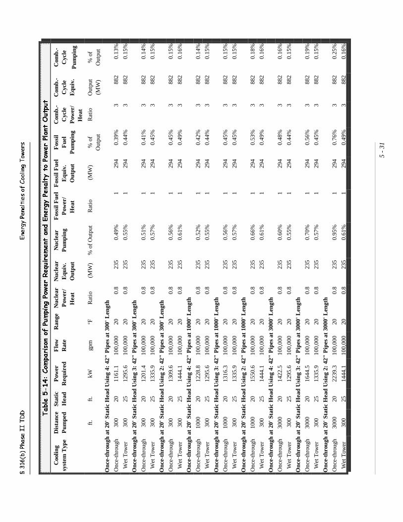
§ 3
16(b
) Ph
ase I
I T
DD
Ene
rgy
Pena
ltie
s of
Coo
ling
Tow
ers
5 -
31
Table 5
-14:
Compariso
n o
f Pumping P
ower
Requirement
and E
nerg
y P
enalty t
o P
ower
Plant
Outp
ut
Coo
ling
syst
em T
ype
Dis
tanc
eP
umpe
dSt
atic
Hea
dP
ower
Req
uire
dF
low
Rat
eR
ange
Nuc
lear
Pow
er/
Hea
t
Nuc
lear
Equ
iv.
Out
put
Nuc
lear
Pum
ping
Fos
sil F
uel
Pow
er/
Hea
t
Fos
sil F
uel
Equ
iv.
Out
put
Fos
sil
Fue
lP
umpi
ng
Com
b.-
Cyc
leP
ower
/H
eat
Com
b.-
Cyc
leE
quiv
.
Com
b.-
Cyc
le
Pum
ping
ft.
ft.
kWgp
mo F
Rat
io (
MW
)%
of
Out
put
Rat
io (
MW
)%
of
Out
put
Rat
ioO
utpu
t(M
W)
% o
fO
utpu
t
Onc
e-th
roug
h at
20'
Sta
tic
Hea
d U
sing
4:
42"
Pip
es a
t 30
0' L
engt
h
Onc
e-th
roug
h30
020
1161
.110
0,00
020
0.8
235
0.49
%1
294
0.39
%3
882
0.13
%
Wet
Tow
er30
025
1295
.610
0,00
020
0.8
235
0.55
%1
294
0.44
%3
882
0.15
%
Onc
e-th
roug
h at
20'
Sta
tic
Hea
d U
sing
3:
42"
Pip
es a
t 30
0' L
engt
h
Onc
e-th
roug
h30
020
1201
.410
0,00
020
0.8
235
0.51
%1
294
0.41
%3
882
0.14
%
Wet
Tow
er30
025
1335
.910
0,00
020
0.8
235
0.57
%1
294
0.45
%3
882
0.15
%
Onc
e-th
roug
h at
20'
Sta
tic
Hea
d U
sing
2:
42"
Pip
es a
t 30
0' L
engt
h
Onc
e-th
roug
h30
020
1309
.610
0,00
020
0.8
235
0.56
%1
294
0.45
%3
882
0.15
%
Wet
Tow
er30
025
1444
.110
0,00
020
0.8
235
0.61
%1
294
0.49
%3
882
0.16
%
Onc
e-th
roug
h at
20'
Sta
tic
Hea
d U
sing
4:
42"
Pip
es a
t 10
00' L
engt
h
Onc
e-th
roug
h10
0020
1228
.810
0,00
020
0.8
235
0.52
%1
294
0.42
%3
882
0.14
%
Wet
Tow
er30
025
1295
.610
0,00
020
0.8
235
0.55
%1
294
0.44
%3
882
0.15
%
Onc
e-th
roug
h at
20'
Sta
tic
Hea
d U
sing
3:
42"
Pip
es a
t 10
00' L
engt
h
Onc
e-th
roug
h10
0020
1316
.310
0,00
020
0.8
235
0.56
%1
294
0.45
%3
882
0.15
%
Wet
Tow
er30
025
1335
.910
0,00
020
0.8
235
0.57
%1
294
0.45
%3
882
0.15
%
Onc
e-th
roug
h at
20'
Sta
tic
Hea
d U
sing
2:
42"
Pip
es a
t 10
00' L
engt
h
Onc
e-th
roug
h10
0020
1550
.610
0,00
020
0.8
235
0.66
%1
294
0.53
%3
882
0.18
%
Wet
Tow
er30
025
1444
.110
0,00
020
0.8
235
0.61
%1
294
0.49
%3
882
0.16
%
Onc
e-th
roug
h at
20'
Sta
tic
Hea
d U
sing
4:
42"
Pip
es a
t 30
00' L
engt
h
Onc
e-th
roug
h30
0020
1422
.510
0,00
020
0.8
235
0.60
%1
294
0.48
%3
882
0.16
%
Wet
Tow
er30
025
1295
.610
0,00
020
0.8
235
0.55
%1
294
0.44
%3
882
0.15
%
Onc
e-th
roug
h at
20'
Sta
tic
Hea
d U
sing
3:
42"
Pip
es a
t 30
00' L
engt
h
Onc
e-th
roug
h30
0020
1644
.510
0,00
020
0.8
235
0.70
%1
294
0.56
%3
882
0.19
%
Wet
Tow
er30
025
1335
.910
0,00
020
0.8
235
0.57
%1
294
0.45
%3
882
0.15
%
Onc
e-th
roug
h at
20'
Sta
tic
Hea
d U
sing
2:
42"
Pip
es a
t 30
00' L
engt
h
Onc
e-th
roug
h30
0020
2239
.310
0,00
020
0.8
235
0.95
%1
294
0.76
%3
882
0.25
%
Wet
Tow
er30
025
1444
.110
0,00
020
0.8
235
0.61
%1
294
0.49
%3
882
0.16
%

§ 316(b) Phase II TDD Energy Penalties of Cooling Towers
5 - 32
Note: Wet Towers are assumed to always be at 300' distance and have the same tower pumping head of 25' in all scenarios shown. The same flow ratecfs) is used for all scenarios. Power/Heat Ratio refers to the ratio of Power Plant Output (MW) to the heat (in equivalent MW) transferred through the
3-1 for the total energy penalties. This table presents only the pumping component of the total energy penalty
§ 316(b) Phase II TDD Energy Penalties of Cooling Towers
5 - 33
5.5.1 Summary of Cooling System Energy Requirements
EPA chose the piping scenario in Table 5-13 where pumping head is close to 50 ft for both once-through and recirculatingsystems at new, “greenfield” facilities (that is, once-through at 1,000 ft and 3-42 in. pipes in Table 5-13). Thus, the coolingwater pumping requirements for once-through and recirculating wet towers are nearly equal using the chosen site-specificconditions. Table 5-15 summarizes the fan and pumping equipment energy requirements as a percent of power output for eachtype of power plant. Table 5-16 presents the net difference in energy requirements shown in Table 5-15 for the alternativecooling systems. The net differences in Table 5-16 are the equipment operating energy penalties associated with conversionfrom one cooling technology to another.
EPA notes that the penalties presented in Tables 5-15 and 5-16 do not comprise the total energy penalties (which incorporateall three components of energy penalties: turbine efficiency penalty, fan energy requirements, and pumping energy usage) asa percent of power output. The total energy penalties are presented in section 5.1 above. The tables below only present thepumping and fan components. Section 5.3.4 presents the turbine efficiency components of the energy penalty.
Table 5-15: Summary of Fan and Pumping Energy Requirements as a Percent of Power
Output
Wet TowerPumping
WetTower
Fan
Wet TowerTotal
Once-throughTotal
(Pumping)
Dry TowerTotal (Fan)
Nuclear 0.57% 0.91% 1.48% 0.56% 3.04%
Fossil Fuel 0.45% 0.73% 1.18% 0.45% 2.43%
Combined-Cycle 0.15% 0.24% 0.39% 0.15% 0.81%
Note: See Section 5.1 for the total energy penalties.
Table 5-16: Fan and Pumping Energy Penalty Associated with Alternative
Cooling System as a Percent of Power Output
Wet Tower VsOnce-through
Dry Tower Vs WetTower
Dry Tower Vs Once-through
Nuclear 0.92% 1.56% 2.48%
Fossil Fuel 0.73% 1.25% 1.98%
Combined-Cycle 0.24% 0.42% 0.66%
Note: See Section 5.1 for the total energy penalties.
§ 316(b) Phase II TDD Energy Penalties of Cooling Towers
5 - 34
5.6 OTHER SOURCES OF ENERGY PENALTY ESTIMATES
The Agency sought out additional sources of energy penalty estimates for its analysis of regulatory options for the316(b) Existing Facility proposal. In part due to the lack of robust, empirical data available, the Agency undertookthe original energy penalty analysis in support of the New Facility Rule. For this Existing Facility proposal the factthat certain regulatory options involved the conversion of aging cooling systems at existing facilities presented anadditional complexity to the Agency. The following sections summarize the Agency’s data collection for estimates ofenergy penalties at existing facilities.
5.6.1 Jefferies Generating Station Energy Penalty Study
As a result of its research for empirical examples of cooling system conversions, the Agency identified an empiricalenergy penalty study associated with the construction of wet, mechanical-draft cooling towers to replace an originalonce-through system. The Jefferies Generating Station -- a 346 MW, coal-fired plant in South Carolina – owned bySantee Cooper, conducted a turbine efficiency loss study in the late 1980s. The facility converted their cooling system(after many years of operation utilizing a once-through system) to a full recirculating, mechanical-draft system around1985. Due to the unusual arrangement whereby the U.S. Army Corps of Engineers (USACE) paid for the constructionand operation of the cooling tower, Santee Cooper began an empirical study to assess the economic impact of theoperation of the cooling towers over the previous once-through system, in order to obtain reimbursement from theUSACE. The study lasted several years (1985 to 1990). However, the empirical stage of data gathering occurredprimarily in 1988. Santee Cooper determined (and the USACE eventually agreed) that the cooling tower had decreasedthe efficiency of each of the plant’s steam turbines. The efficiency penalties determined by Santee Cooper were amaximum of 0.97 percent of plant capacity (for both units, combined) and an annual average of 0.16 percent for theyear 1988. Note, that because the USACE maintains and pays for the operation of the cooling towers, Santee Cooperonly examined the turbine portion of the energy penalty at the plant. The Agency requested documentation on thehistoric operation of the towers from the USACE (in addition to the construction costs from 1986) but did not receivethis information at the time of publication of this proposal. The study conducted by Santee Cooper is included in therecord of today’s proposal (see DCN 4-2527). The Agency notes that its fossil-fuel estimate for the national-average,peak-summer, turbine energy penalty is 0.90 percent and the mean-annual, national-average energy penalty is 0.35percent (at 100 percent of maximum load). For the model plant in Jacksonville, Florida the Agency calculated a fossil-fuel peak-summer turbine energy penalty of 0.61 percent and the mean-annual turbine energy penalty of 0.38 percent(at 100 percent of maximum load).
5.6.2 U.S. Department of Energy Peak-Summer Energy Penalty Study
The U.S. Department of Energy (DOE), through its Office of Fossil Energy, National Energy Technology Laboratory(NETL), and Argonne National Laboratory (ANL), studied the energy penalty resulting from converting plants withonce-through cooling to wet towers or indirect dry towers. DOE modeled five locations – Delaware River Basin(Philadelphia), Michigan/Great Lakes (Detroit), Ohio River Valley (Indianapolis), South (Atlanta), and Southwest(Yuma) – using an ASPEN simulator model. The model evaluated the performance and energy penalty for hypothetical400-MW coal-fired plants that were retrofitted from using once-through cooling systems to indirect-wet- and indirect-dry-recirculating systems. The modeling was done to simulate the hottest time of the year using temperature inputvalues that are exceeded only 1 percent of the time between June through September at each modeled location. AtDOE’s request, EPA provided, discharge temperature data and thermal discharge permit limits for facilities at or nearthe DOE study locations for use in the model. EPA also provided comments regarding the framework of the modelingproject, which are included in the record of this proposal (see DCN 4-2512)
§ 316(b) Phase II TDD Energy Penalties of Cooling Towers
5 - 35
After completing their initial modeling, DOE shared the results of their working draft report with the EPA, which isincluded in the record of this proposal (see DCN 4-2511). DOE estimates that conversion to a wet tower could causepeak-summer energy penalties ranging from 2.8 percent to 4.0 percent. Therefore, DOE estimates that the plant willproduce 2.8 percent to 4.0 percent less electricity with a wet tower than it did with a once-through system while burningthe same amount of coal. Further, DOE estimates that conversion to an indirect-dry tower could cause peak-summerenergy penalties ranging from 8.9 percent to 14.1 percent with a design approach of 20 degrees Fahrenheit and 12.7percent to approximately 18 percent with an approach of 40 degrees Fahrenheit.
EPA did not model indirect-dry cooling systems, and therefore cannot directly compare its estimates to those developedby DOE. However, EPA can compare its estimates of peak summer energy penalties for mechanical draft wet coolingtowers to those developed by DOE. The Agency finds that its estimates of peak summer energy penalties aresignificantly lower than those developed by DOE (see section 5.1 for EPA’s estimates of peak summer energy penaltiesof mechanical draft cooling towers). EPA and DOE believe that the difference in these estimates is most likely due totwo key factors: (1) the estimated energy penalty attributable to the parasitic energy use of cooling water pumps and(2) the estimated design temperature ranges of cooling water from condenser inlet to outlet.
As discussed at Section 5.3 above, EPA developed energy penalty estimates for this proposal based on its estimates forthe 316(b) New Facility Rule. For the energy penalty estimates of the 316(b) New Facility Rule, the Agency conductedan analysis of a variety of pumping scenarios for once-through versus recirculating systems at new “greenfield”facilities. The Agency concluded that for “greenfield” facilities, the cooling towers would generally be sited in closeproximity to condenser units. Therefore, the Agency estimated that pumping distances for recirculating systems wouldbe significantly less than those for once-through systems. (The Agency provided this analysis for public comment inthe June 2001 Notice of Data Availability). In the analysis of energy penalties for new, “greenfield” plants, the Agencyconcluded that the difference in pumping distance for a once-through system would offset the additional static headpumping requirements of a typical mechanical draft cooling tower (see section 5.4.2 for the Agency’s analysis ofpumping energy requirements). Therefore, the analysis of energy penalties used by the Agency for this proposalestimates 0.0 percent energy penalty due to pumping requirements. DOE, on the other hand, estimates that a retrofittedwet cooling tower would require significantly more pumping energy than a baseline, once-through cooling system. Theresults of the DOE study show pumping energy penalties ranging from 0.2 to 0.7 percent. The Agency views the DOEestimates to be reasonable for a variety of retrofit scenarios at existing facilities and will reconsider this subject in theanalysis of regulatory options for the final rule.
While EPA did not directly estimate design temperature range in its modeling approach, in effect DOE and EPA useddifferent design temperature ranges, which can dramatically affect energy penalty estimates. The DOE modelingapproach used simulated inlet and discharge water temperatures for the chosen sites. EPA provided thermal dischargepermit information, which DOE incorporated into a parametric analysis of design temperature ranges (that is, DOEexamined a variety of temperature ranges, from 5 degrees F to 25 degrees F). For example, the design ranges examinedby DOE for their Michigan site show peak energy penalties that vary by 1 percent, from 3.95 % for a 7 degree F designrange to 2.94 % for a 25 degree F design range. In the case of other model sites, such as Georgia, a design rangeincrease of 5 degrees F (from 5 degrees F to 10 degrees F) can dramatically effect the results of the energy penaltyestimates. The DOE model estimates a 3.99 % percent energy penalty for the 5 degrees F design range in Georgia and2.78 % for the 10 degrees F design range assumption. As EPA noted in its comments on DOE’s proposed energypenalty analysis, EPA believes that design temperature ranges of less than 13 degrees F are not realistic at most
§ 316(b) Phase II TDD Energy Penalties of Cooling Towers
5 - 36
locations and are likely to lead to energy penalty estimates that are higher than would occur under realistic operatingconditions.
In addition to the two key factors described above, DOE expressed concern to EPA that the Agency’s modeling analysisof turbine energy penalties did not incorporate subtle effects on the condenser duty. Specifically, DOE did not believethat the Agency’s model takes into account the increase in turbine exhaust temperature (or steam temperature tocondenser) resulting from a corresponding increase in condenser duty when changing the once-through cooling watersystem to a wet cooling tower. Under peak energy penalty periods, the temperature of the condenser cooling water willbe greater under wet cooling tower operation then the same plant operated under once-through cooling because of thedifference between ambient wet-bulb and surface water temperatures. DOE believes that the increased condenser dutyfor the wet cooling tower results in an increase in cooling water flow which increases the cooling water pump andcooling tower fan energy penalties compared to the Agency’s approach.
DOE also points out that the Agency's model does not consider a second effect that since the steam is condensed at aslightly higher temperature for the wet cooling tower case, the reheating of the recirculated steam condensate willrequire a reduction in the amount of steam bleed from the turbine system. This results in a slightly higher steamflowrate through the turbines and into the condenser. This again increases the condenser duty and would again increasethe parasitic energy penalties. However, this would probably be offset by an increase in power due to a small increasein the steam flowrate in the turbines. DOE estimates that these effects may contribute a maximum of 0.5 percentagepoints to the Agency ‘s evaluation of the peak-summer energy penalty.
5.6.3 Catawba and McGuire Nuclear Plant Comparison
One literature source the Agency encountered calculated the energy penalty of a nuclear plant employing a mechanical-draft wet cooling system by comparing the electrical ratings of the Catawba and McGuire Nuclear Plants. Becausethe two plants were constructed nearly identically, the author hypothesized that the percent difference electrical ratingbetween the two plants would represent the energy usage of a cooling tower. The Agency notes that even though acomparison of this type would theoretically calculate the net energy use of the pumps and fans of the wet cooling towersystem as compared to the once-through system, there are a variety of complicating factors that are not accounted foror are overlooked in this case. The electrical rating of a nuclear plant does not, to the Agency’s knowledge, accountfor the turbine efficiency penalty component. This key portion of the energy penalty would not be included in theelectrical rating calculations of the plant. The comparison could, therefore, underestimate the total energy penalty ofthe cooling system.
Nonetheless, the Agency examined the historical energy penalty estimate for the Catawba versus McGuire case anddetermined that the source had made an error in calculating an estimate of 3 percent for the overall energy use of thecooling towers over the once-through system. The error made was to assume that each plant had the same grosscapacity. In fact, the McGuire plant has a gross capacity that is 31 MW greater than Catawba. Therefore, acomparison of the percentage difference between gross and net capacity for the two plants actually should be calculatedas 1.7 percent. This energy penalty estimate for the fan and pumping components is higher than that estimated by theAgency elsewhere in this chapte for nuclear facilities. The Agency estimates that the total of the fanning and pumpingcomponents for a nuclear plant would be 0.9 percent. As described in Section 5.3 of this chapter, the Agency’sestimates of the pumping components developed for new, “greenfield” facilities calculate no net change in the pumping
§ 316(b) Phase II TDD Energy Penalties of Cooling Towers
1 The EPA calculations for energy penalties specific to Palisades and Lake Michigan utilized the data from the 2001Consumers Energy permit document with the energy penalty methodology outlined in this chapter.
5 - 37
requirements between once-through and recirculating wet cooling tower systems. As stated in Section 5.6.2 above, thismay also explain to some degree the differences between the Agency’s and the Catawba/McGuire estimate.
5.6.3 Palisades Cooling System Conversion Energy Penalty Estimate
The Agency learned from discussions with, and information submitted by, Consumers Energy that the cooling towersystem at Palisades might have a significant impact on the efficiency of the plant’s generating unit. Though the plantwas unable to provide historical studies of the energy penalty of the cooling tower system, they estimate that the effectcould be approximately 7 percent (Gulvas, 2002). Prior to the 1970’s conversion, the Nuclear Regulatory Commission(NRC) estimated that the cooling tower system would affect plant efficiency by 3 percent (Gulvas, 2002). ConsumersEnergy estimates that the cooling system fans utilize 4 MW of electricity for operation, and the circulating and intakepumps utilize approximately 16 MW and 3 MW, respectively (Gulvas, 2002). Consumers Energy further estimate thatthe cooling tower system reduces the efficiency of the steam turbine by 6 to 8 percent compared to the original once-through system. Consumers Energy did not provide supporting documentation for the turbine efficiency penalties orpumping and fanning losses as submitted to the Agency.
Based on the Agency’s energy penalty methodology, the turbine energy penalty for a nuclear unit (at peak summerconditions) would be approximately 1.4 percent (11.3 MW for Palisades). The Agency calculated this penalty usingthe historic cooling water temperature data for Palisades provided by Consumers Energy and ambient dry bulb and wetbulb air temperatures specific to Chicago, IL (Consumers, 2001).1 This estimate of turbine efficiency penalty issubstantially less than that estimated by Consumers Energy. The Agency notes that Consumers Energy did not estimatethe original pumping requirements of the once-through system, and, therefore, the net energy penalty (that is, wetcooling tower energy use less the once-through system energy use) of the conversion estimated by Consumers Energymay not be the appropriate comparison. The Agency also notes that the electricity usage of 36-200 hp fans would be5.4 MW with each fan at full operation, slightly higher than the estimate by Consumers Energy. EPA also estimatedthe pumping energy penalty for the recirculating system at Palisades and compared this to the pumping energy requiredfor the former once-through operation of the plant. EPA determined, conservatively (that is, erring on the high side),that the circulating pumping requirements of the cooling tower system currently in place at Palisades would requireapproximately 7.5 MW (that is, 8.5 MW less than the estimate given by Palisades above). The original once-throughsystem would have required approximately 5 MW to convey water 3,300 feet from the offshore intake through 11 ftdiameter pipe, through the condenser, and to discharge at the lake shore. The Agency did not analyze the “dilution”pumping requirements estimated by Consumers Energy as 3 MW above. Therefore, the Agency estimates that the totalenergy penalty of the recirculating tower system at Palisades may have a peak energy penalty close to 2.7 percent andan annual penalty approaching 1.8 percent as compared to the original once-through system (Sunda, et al., 2002).

§ 316(b) Phase II TDD Energy Penalties of Cooling Towers
5 - 38
REFERENCES
Air Force Combat Climatology Center in Ashville, NC. CD entitled Engineering Weather Data (2000 InteractiveEdition). National Climatic Data Center.
Burns, J. M. and W. C. Micheletti. November 2000. Comparison of Wet and Dry Cooling Systems for CombinedCycle Power Plants. Version 2.1. Submitted as Appendix F to the comments of the Utility Water Act Group on EPA’sProposed Section 316(b) Rule for New Facilities.
Consumers Energy Company and Nuclear Management Corporation, May 2001, “Biological Assessment of the 1999Cooling Water Flow Increase at the Palisades Nuclear Plant, near South Haven, Michigan.”
Durand, A et al. May 1999. Updated Rules for Pipe Sizing. Chemical Engineering.
Entergy Nuclear Generation Company (Entergy). February 2001. Condenser Performance Analysis - AdditionalData; Pilgrim Nuclear Power Station. Submitted by J.F. Alexander, to Nicholas Prodany, EPA Region 1.
Environmental Protection Agency. September 2001. The Emissions & Generation Resource Integrated Database2000 (E-GRID 2000). Version 2.0. http://www.epa.gov/airmarkets/egrid/index.html
Fleming, Robert. 2001. Personal communications between Robert Fleming, The Marley Cooling Tower Co., andFaysal Bekdash, SAIC.
General Electric. No Date. Steam Turbine Technology. Field Engineering Development Center Mechanical &Nuclear.
Gulvas, J. A., 2002, “The Palisades Plant Once-through and Cooling Towers,” Consumers Energy data submissionto the U.S. EPA. February 28, 2002.
Heat Exchanger Systems, Inc (HES). 2001. Condenser Performance Analysis.
Hensley, J.C. 1985. Cooling Tower Fundamentals. 2nd Edition. The Marley Cooling Tower Company (Mission,Kansas).
Hess, Dale. June 2001. Condenser Cost Study. Graham Corporation.
Ishigai, S. 1999. Steam Power Engineering - Thermal Hydraulic Design Principles. Cambridge university Press. UK.
Kirk-Othmer. 1997. Encyclopedia of Chemical Technology. Fourth Edition. Volume 22. John Wiley and Sons, Inc.New York.

§ 316(b) Phase II TDD Energy Penalties of Cooling Towers
5 - 39
Litton, T.R. Stanley Consultants, Inc. No Date. “Application of Parallel wet and Dry Condensing Systems to a 35MW Steam Turbine.”
Mirsky, Gary. 2001. Personal communications between Gary Mirsky, Hamon Cooling Towers, and Faysal Bekdash,SAIC.
Nuclear Regulatory Commission. 1996. Generic Environmental Impact Statement for License Renewal of NuclearPlants. NUREG-1437 Vol. 1. http://www.nrc.gov/docs/nuregs/staff/sr1437/V1/sr1437v1.html#_1_128
Perry, W. J., 1991, “Adverse Impact Study; Cooling Water Facilities - Jefferies Generating Station,” for Santee Cooper,Moncks Corners, South Carolina.
Sunda, J.B., et al., 2002, “Analysis of Palisades Nuclear Plant Pumping Energy Requirements.”
Tallon, B. Not Dated. GEA Power Systems Inc. Telephone Contact with John Sunda, SAIC. Regarding Air CooledCondenser Fans.
Tatar, G. October 2001. Telephone Contact with John Sunda, SAIC. Regarding operation of the air cooled condenserfans. El Dorado Energy.
Taylor, S. May 2001. Telephone Contact with John Sunda, SAIC. Regarding cooling water pumping and condenseroperation. Bechtel.
U.S. Department of Energy. May 2000. Statement of Jay E. Hakes Administrator, Energy Information Administration,Department of Energy before the Committee on Energy and Natural Resources, United States Senate.
U.S. Department of Energy. August 2001. “Energy Penalty Analysis on Possible Cooling Water Intake StructureRequirements on Existing Coal-Fired Power Plants,” Working Draft, Office of Fossil Fuel Energy, National EnergyTechnology Laboratory, and Argonne National Laboratory.
U.S. Environmental Protection Agency. April 2001. Memorandum from Tim Connor to Tom Feeley (U.S. Departmentof Energy). “Comments on Proposed Energy Penalty Analysis.”
Woodruff, E.B., Lammers, H.B., Lammers, T.F. 1998. Steam Plant Operation. Seventh Edition. McGraw-Hill. NewYork.

§ 316(b) Phase II TDD Attachments to Chapter 5
Attachm ents
ATTACHMENT A TO CHAPTER 5: HEAT DIAGRAM FOR STEAM
POWER PLANT
(Source: Ishigai 1999)
See Hard Copy
§ 316(b) Phase II TDD Attachments to Chapter 5
Attachm ents
ATTACHMENT B TO CHAPTER 5: EXHAUST PRESSURE
CORRECTION FACTORS
FOR A NUCLEAR POWER PLANT (Attachment B-1)
(Source: Entergy 2001)
See Hard Copy
FOR A FOSSIL FUEL PLANT (Attachment B-2)
(Source: General Electric. Steam Turbine Technology)
See Hard Copy
FOR A COMBINED CYCLE PLANT (Attachment B-3)
(Source: Litton)
See Hard Copy

§ 316(b) Phase II TDD Attachments to Chapter 5
Attachm ents
ATTACHMENT C TO CHAPTER 5: DESIGN APPROACH DATA FOR
RECENT COOLING TOWER PROJECTS
(Source: Mirsky 2001)
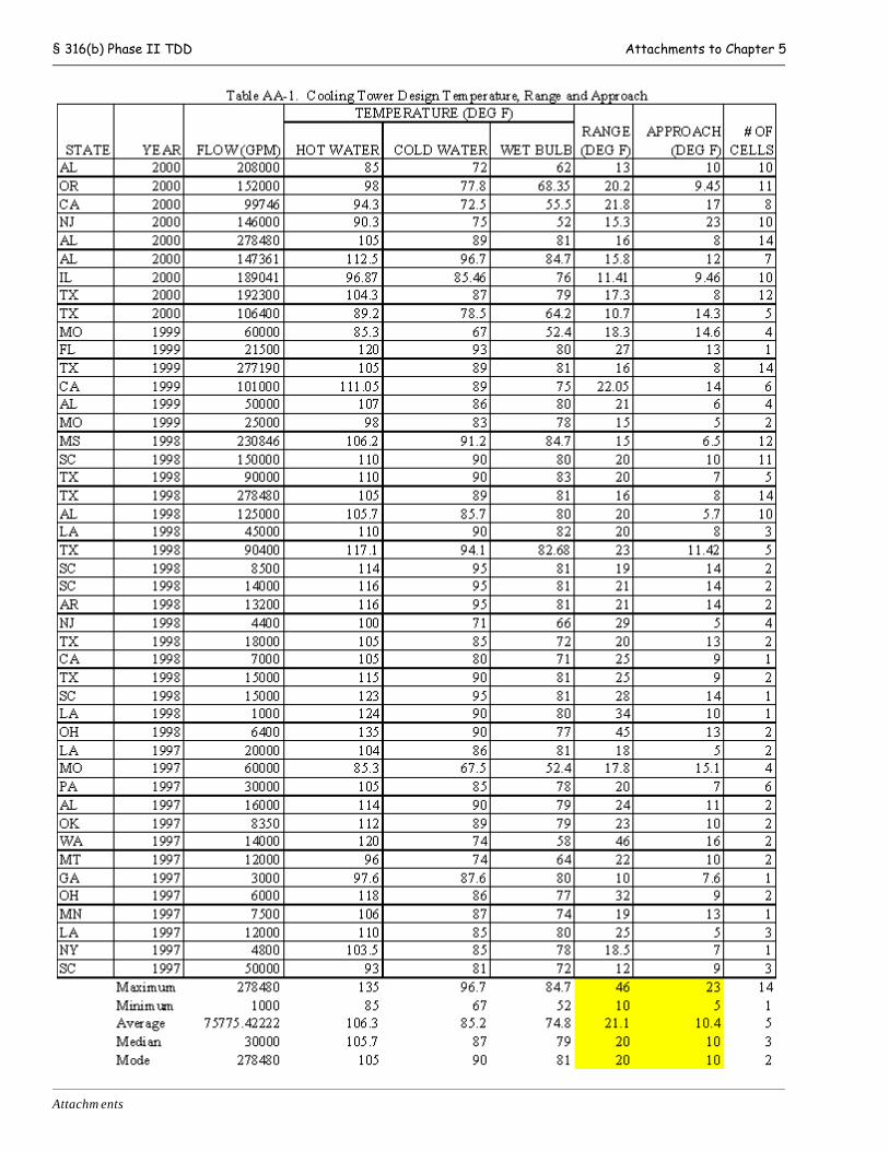
§ 316(b) Phase II TDD Attachments to Chapter 5
Attachm ents

§ 316(b) Phase II TDD Attachments to Chapter 5
Attachm ents
ATTACHMENT D TO CHAPTER 5: TOWER SIZE FACTOR PLOT
(Source: Hensley 1985)
See Hard Copy
§ 316(b) Phase II TDD Attachments to Chapter 5
Attachm ents
ATTACHMENT E TO CHAPTER 5: COOLING TOWER WET BULB VERSUS
COLD WATER TEMPERATURE TYPICAL PERFORMANCE CURVE
(Source: Hensley 1985)
See Hard Copy
§ 316(b) Phase II TDD Non-water Quality Impacts
6 - 1
Chapter 6: Non-Water Quality Impacts
INTRODUCTION
This chapter discusses side effects of the operation of recirculating wet cooling towers including increased air
emissions due to energy penalties, vapor plumes, noise, salt or mineral drift, water consumption through evaporation,
and solid waste generation due to wastewater treatment of tower blowdown.
6.1 AIR EMISSIONS INCREASESDue to recirculating wet cooling system energy penalties, as described in Chapter 5, EPA estimates that air emissions
may marginally increase from power plants that retrofit from once-through to recirculating wet cooling systems. The
energy penalties reduce the efficiency of the electricity generation process and increase auxiliary power consumption;
thereby increasing the quantity of fuel consumed per unit of electricity generated. EPA assumes facilities will seek
to compensate for the energy penalties and maintain their electricity generation levels because of contractual
obligations and market conditions. EPA believes the facili ties will be capable of compensating for the energy
penalties based on its analysis of unused capacity in the industry. EPA presents the estimates of annual air emissions
increases under the flow reduction-waterbody option (Option 1) in Table 6-1 below. This analysis describes
estimated increases only for Option 1.
EPA developed estimates of incremental increases in air emissions of carbon dioxide (CO2), mercury (Hg), sulfur
dioxide (SO2), nitrogen oxides (NOx), and particulate matter (PM2.5 and PM10) for the facilities projected to
upgrade their cooling systems under the flow reduction-waterbody option in today’s proposed rule. These facilities
include nuclear, combined-cycle, and fossil fuel-fired power plants. Generally, combined-cycle plants produce
significantly less air emissions per kilowatt-hour of electricity generated than fossil fuel-fired plants. Because a
combined-cycle plant requires cooling for approximately one-third of its process (on a megawatt capacity basis) and
because of the differences in combustion products from natural gas versus other fossil fuels, the combined-cycle plant
produces less air emissions than fossil fuel-fired plants, even after such plants are equipped with state-of-the-art
emissions controls. Nuclear power plants utilize radioactive materials as fuel and have extremely low or negligible
emission rates of CO2, Hg, SO2, NOx, PM2.5, and PM10 in comparison to those found at either combined-cycle or
fossil fuel-fired facilities.
EPA assumed that a facility incurring an energy penalty from retrofitting a once-through cooling system to a
recirculating wet cooling system would seek to compensate for that penalty by increasing their electricity generation
and would be able to do so by increasing electricity generation on-site. Most facilities do not operate at full
electricity generation capacity on an annual basis. EPA believes such facilities would be able to compensate on an
annual basis for the annual energy penalty due to conversion to a recirculating wet cooling system by increasing on-
site electricity generation.
EPA could alternatively assume that plants incurring an energy penalty will not increase their fuel consumption on-
site to overcome incurred energy penalties. Instead, facilities affected by the requirements of this rule would
purchase replacement power from the grid. Under this scenario, the air emissions increases associated with a
particular energy penalty at an affected plant would be released by the rest of the grid as a whole, thereby comprising
§ 316(b) Phase II TDD Non-water Quality Impacts
6 - 2
small increases at a large number and variety of power plants. During the development of the Section 316(b) Final
Rule addressing new facilities, EPA received comments asserting that not all facilities, especially during times of
peak demand, would be able to increase their fuel consumption to overcome energy penalties. Nuclear facilities, in
particular, may not be able to increase generation on-site. EPA has not calculated the national marginal increase in
air emissions associated with purchase of electricity from the grid, though it notes that such purchases are a possible
outcome of cooling system conversions. The Agency believes that the outcome of a national analysis would be
similar to that of the facility-specific analysis because the distribution of facility types and their associated emissions
profiles in each analysis would be comparable.
The estimated air emissions increases presented in Table 6-x below represent facility-specific increases and are based
on the estimated energy penalty for each facility, the facility’s historic average electricity generation level, and its
average historic emission rates. The data source for the Agency’s air emissions estimates of CO2, SO2, NOX, and Hg
is the EPA-developed database titled E-GRID 2000. This database is a compendium of reported air emissions, plant
characteristics, and industry profiles for the entire US electricity generation industry in the years 1996 through 1998.
The database relies on information from power plant emissions reporting data from the Energy Information
Administration of the Department of Energy. The database compiles information on every major power plant in the
United States and includes statistics such as plant operating capacity, air emissions, electricity generated, fuel
consumed, etc. This database provided ample data for the Agency to conduct air emissions increases analyses for
this rule. The emissions reported in the database are for the power plants’ actual emissions to the atmosphere and
represent emissions after the influence of air pollution control devices. To test the veracity of the database for the
purposes of this rule, the Agency compared the information to other sources of data available on power plant
capacities, fuel-types, locations, owners, and ages. Without exception, the E-GRID 2000 database provided accurate
estimates of each of these characteristics versus information that EPA was able to obtain from other sources. E-GRID
2000, however, does not provide information on emissions of particulate matter. The data source for historic
emissions rates of PM2.5 and PM10 is the EPA-developed database titled National Emission Trends (NET). The
NET database is an emission inventory that contains data on stationary and mobile sources that emit criteria air
pollutants and their precursors. The NET is released every three years (e.g., 1996 and 1999) and includes emission
estimates for all 50 States, the District of Columbia, Puerto Rico, and the Virgin Islands. The database compiles
information from EPA air programs and the Department of Energy, and the information it contains was found to be
consistent with the information found in E-GRID 2000.
A facility that increases on-site electricity generation to compensate for the energy penalty associated with retrofitting
its cooling water system may, because of the resultant on-site increase in air pollutant emissions, be subject to new
source review (NSR). Major stationary sources of air pollution undergoing major modifications are required by the
Clean Air Act to obtain an air pollution permit before commencing construction. The process is called new source
review and is required whether the major source or modification is planned for an area where the national ambient
air quality standards (NAAQS) are exceeded (nonattainment areas) or an area where air quality is acceptable
(attainment and unclassifiable areas).
There are costs associated both with undergoing NSR and with measures taken to ensure compliance with new air
emission control requirements delineated during the NSR process. If a facility purchases electricity from the grid,
it does not need to undergo NSR and can therefore avoid the associated costs. EPA believes that some facilities
retrofitting their cooling systems under the proposed regulatory alternative requiring flow reduction commensurate
with closed cycle wet cooling based on water body type may choose to purchase energy from the grid rather than
incur the costs associated with NSR. The resulting increase in emissions would be similar to that estimated given
on-site generat ion of additional electricity.
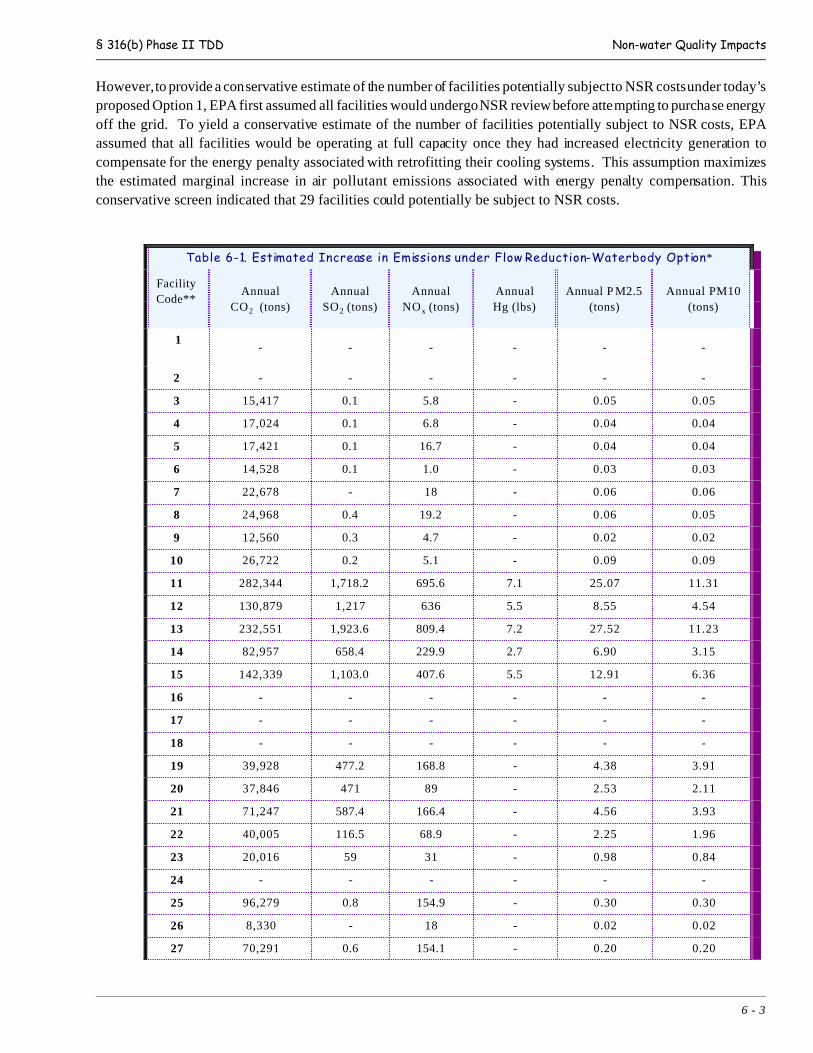
§ 316(b) Phase II TDD Non-water Quality Impacts
6 - 3
However, to provide a conservative estimate of the number of facilities potentially subject to NSR costs under today’s
proposed Option 1, EPA first assumed all facilities would undergo NSR review before attempting to purchase energy
off the grid. To yield a conservative estimate of the number of facilities potentially subject to NSR costs, EPA
assumed that all facilities would be operating at full capacity once they had increased electricity generation to
compensate for the energy penalty associated with retrofitting their cooling systems. This assumption maximizes
the estimated marginal increase in air pollutant emissions associated with energy penalty compensation. This
conservative screen indicated that 29 facilities could potentially be subject to NSR costs.
Table 6-1. Estimated Increase in Emissions under Flow Reduction-Waterbody Option*
Facility
Code**Annual
CO2 (tons)
Annual
SO2 (tons)
Annual
NOx (tons)
Annual
Hg (lbs)
Annual P M2.5
(tons)
Annual PM10
(tons)
1- - - - - -
2 - - - - - -
3 15,417 0.1 5.8 - 0.05 0.05
4 17,024 0.1 6.8 - 0.04 0.04
5 17,421 0.1 16.7 - 0.04 0.04
6 14,528 0.1 1.0 - 0.03 0.03
7 22,678 - 18 - 0.06 0.06
8 24,968 0.4 19.2 - 0.06 0.05
9 12,560 0.3 4.7 - 0.02 0.02
10 26,722 0.2 5.1 - 0.09 0.09
11 282,344 1,718.2 695.6 7.1 25.07 11.31
12 130,879 1,217 636 5.5 8.55 4.54
13 232,551 1,923.6 809.4 7.2 27.52 11.23
14 82,957 658.4 229.9 2.7 6.90 3.15
15 142,339 1,103.0 407.6 5.5 12.91 6.36
16 - - - - - -
17 - - - - - -
18 - - - - - -
19 39,928 477.2 168.8 - 4.38 3.91
20 37,846 471 89 - 2.53 2.11
21 71,247 587.4 166.4 - 4.56 3.93
22 40,005 116.5 68.9 - 2.25 1.96
23 20,016 59 31 - 0.98 0.84
24 - - - - - -
25 96,279 0.8 154.9 - 0.30 0.30
26 8,330 - 18 - 0.02 0.02
27 70,291 0.6 154.1 - 0.20 0.20
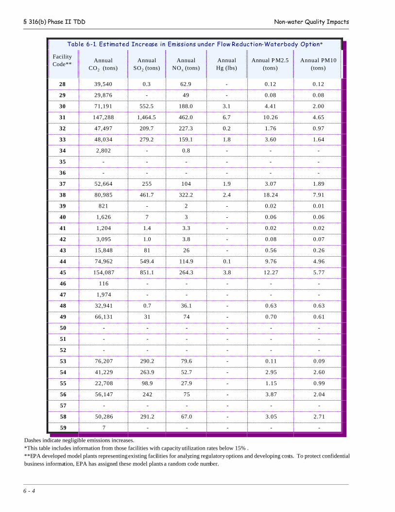
§ 316(b) Phase II TDD Non-water Quality Impacts
Table 6-1. Estimated Increase in Emissions under Flow Reduction-Waterbody Option*
Facility
Code**Annual
CO2 (tons)
Annual
SO2 (tons)
Annual
NOx (tons)
Annual
Hg (lbs)
Annual P M2.5
(tons)
Annual PM10
(tons)
6 - 4
28 39,540 0.3 62.9 - 0.12 0.12
29 29,876 - 49 - 0.08 0.08
30 71,191 552.5 188.0 3.1 4.41 2.00
31 147,288 1,464.5 462.0 6.7 10.26 4.65
32 47,497 209.7 227.3 0.2 1.76 0.97
33 48,034 279.2 159.1 1.8 3.60 1.64
34 2,802 - 0.8 - - -
35 - - - - - -
36 - - - - - -
37 52,664 255 104 1.9 3.07 1.89
38 80,985 461.7 322.2 2.4 18.24 7.91
39 821 - 2 - 0.02 0.01
40 1,626 7 3 - 0.06 0.06
41 1,204 1.4 3.3 - 0.02 0.02
42 3,095 1.0 3.8 - 0.08 0.07
43 15,848 81 26 - 0.56 0.26
44 74,962 549.4 114.9 0.1 9.76 4.96
45 154,087 851.1 264.3 3.8 12.27 5.77
46 116 - - - - -
47 1,974 - - - - -
48 32,941 0.7 36.1 - 0.63 0.63
49 66,131 31 74 - 0.70 0.61
50 - - - - - -
51 - - - - - -
52 - - - - - -
53 76,207 290.2 79.6 - 0.11 0.09
54 41,229 263.9 52.7 - 2.95 2.60
55 22,708 98.9 27.9 - 1.15 0.99
56 56,147 242 75 - 3.87 2.04
57 - - - - - -
58 50,286 291.2 67.0 - 3.05 2.71
59 7 - - - - -
Dashes indicate negligible emissions increases.
*This table includes information from those facilities with capacity utilization rates below 15% .
**EPA developed model plants representing existing facilities for analyzing regulatory options and developing costs. To protect confidential
business information, EPA has assigned these model plants a random code number.
§ 316(b) Phase II TDD Non-water Quality Impacts
1 November 2001, “Hearing Report and Recommended Decision by State of New York, in the Matter of Mirant Bowline,
LLC, Application for a State Pollutant Discharge Elimination System.” The report states, “Mirant has explained that the
primary reason for revising the cooling/intake proposal is to reduce cooling tower steam plumes, thereby further reducing
adverse visual impacts of the project.” 2 Note: the 3 16(b) N ew Facility Rule estimated tha t nine-new, “gree nfield” facilities ov er a twenty year p eriod wo uld comp ly
with the rule by installing wet cooling towers. However, the New Facility rule did not mandate a compliance technology and
provides flexible compliance options through a multi-track framework.3 Chapter 3 of the Technical Development Document of the Final Regulations Addressing Cooling Water Intake Structures for
New Facilities.
6 - 5
6.2 VAPOR PLUMES
Natural draft or mechanical draft cooling towers can produce vapor plumes. Plumes can create problems for fogging
and icing, which have been recorded to create dangerous conditions for local roads and for air and water navigation.
Plumes are in some cases disfavored for reasons of aesthetics. Generally, mechanical draft cooling towers have
significantly shorter plumes than those for natural draft towers (by approximately 30 percent).
As discussed in Chapter 4, the Agency considered regulatory options based on flow reduction commensurate with
closed-cycle wet cooling systems. The Department of Energy (DOE) expressed concern to the Agency that plume
abatement technologies would be required for a subset of existing plants projected to adopt wet cooling towers under
these options. The DOE believed that the options based on flow reduction should consider a significant portion of
existing facilities converting from once-through systems to hybrid wet/dry cooling towers, instead of the wet (only)
towers examined by the Agency.
Historical ly, plants have adopted plume reduction technologies for the following reasons: visual aesthetics,1 liability
relating to icing and fogging of nearby transportation routes (US EPA Reg I, 2002), and potentially elevated moisture
levels affected nearby agriculture. For the 316(b) New Facility Final Rule, the Agency considered plume effects of
wet cooling towers. The Agency determined that for the limited number of new, “greenfield” facilities that may adopt
towers to meet the flow reduction requirements of the rule,2 that the plume effects would not be a sufficient
environmental concern, especially in comparison to the significant aquatic environmental benefits of intake flow
reduction.3 However, in the Agency’s view, the issue of vapor plume effects at existing facilities requires a slightly
different consideration. Existing facilities do not have the advantage of siting and designing the plant layout to
minimize plume effects, which is far and away the most economic means of plume mitigation. Through the
utilization of terrain features, buffer areas, prevailing wind directions, and site selection, the new, “greenfield” facility
has a set of tools that provide a distinct advantage for plume mitigation over an existing plant converting its cooling
system. Therefore, the Agency examined historic studies and example cases of plumes and plume mitigation to
understand the prevalence and necessity of plume abatement for cooling tower installations at existing facilities.
Hybrid wet/dry tower systems are the technology most frequently associated with plume abatement. The primary
type of wet/dry tower employed in practice is a configuration where an air-cooled condensing unit sits atop a wet
evaporative unit. This technology, in effect, reduces the amount of moisture transferred to the air by raising the
temperature and lowering the relative humidity of the exhaust air. The heated water from the condensers is fed first
to the top, dry portion of the tower, where air flows around the air-cooled condenser and heat transfers to the
environment without evaporation of water. The water then disperses through the wet portion of the system, where
heat transfer from the water to the air occurs primarily through the more efficient means of evaporation. Because
the air-cooled portion creates an elevated temperature environment for the exhaust plume and reduces the temperature
of the water before entering the evaporative section, the frequency and extent of the exhaust vapor plume is reduced.
The air-cooled portion of the hybrid-wet/dry tower is relatively inefficient in comparison to the wet-cooled system,
§ 316(b) Phase II TDD Non-water Quality Impacts
4 Power Tech Associates (1999) state, when referring to their estimates of cooling system conversion costs for the four
Hudson River plants, “the effect of using wet/dry towers is much less than a 25 percent increase in the overall conversion
costs.”
6 - 6
and the overall efficiency of the hybrid system is reduced compared to a wet (only) cooling tower. However,
advances in the design of the hybrid tower systems allow bypassing of the air-cooled condenser portion, thereby
allowing the tower to function in the more efficient wet (only) cooling mode when the meteorological conditions do
not favor visual plume formation or electricity demand requires maximum capacity of the plant (BDT Engineering,
2000) (US EPA Reg I, 2002). The Agency notes that the type of hybrid tower used for plume abatement generally
does not reduce water intake compared to a wet cooling tower and would, therefore, have no appreciable reduction
in the potential aquatic impacts of cooling water intakes. In addition, the technology may, through the fact that it is
less efficient than a wet (only) cooling tower system, cause the plant to emit more air pollutants due to the energy
penalty as compared to a wet cooling tower system and a once-through system.
The ratio of the capital cost of the hybrid tower systems (alone, without the necessary and costly auxiliary
components such as piping, pumps, etc.) to the cost of wet (only) towers (without necessary, auxiliary components)
generally is on the order of 2.0 to 3.0 (Mirsky, et al., 1992) (Power Tech Associates, 1999). For a typical new facility
installation, including all of the auxiliary components of yard piping, pumps and motors, basin, sump, electrical
wiring and controls, excavation, site preparation, water treatment, etc., the cooling tower unit will comprise a portion
of the total capital costs. The Utility Water Act Group, in comments submitted to the Agency for the 316(b) New
Facility Proposed Rule presented wet (only) cooling tower unit costs as approximately 45 percent of the total cooling
tower system direct capital costs and approximately 35 percent of total estimated costs (Burns and Michiletti, 2000).
Several turnkey costs that the Agency received from cooling tower engineering firms showed the wet cooling tower
unit portion of total project costs varied from approximately 25 to 40 percent. The Agency expects that the hybrid
wet/dry tower would not appreciably affect the auxiliary component costs of a full cooling tower installation.
Therefore, the Agency concludes that hybrid wet/dry tower unit would increase the overall capital costs for the total
cooling tower system (including all auxiliary components) at a new, “greenfield” facility by approximately 25 to 80
percent as compared to a wet (only) unit. For cooling systems conversions, the Agency estimates that the cooling
tower unit would be identical to that of a new, “greenfield” facility, but that the auxiliary components would be
considerably more expensive. The Agency estimates that the overall cooling tower project costs would be roughly
20 percent more expensive, due mostly to the increase in costs of the auxiliary components. Hence, for existing-
facility cooling tower retrofits, the Agency estimates the increase in overall project cost for a hybrid wet/dry cooling
tower unit over a wet (only) unit would range between 20 and 65 percent.4
As stated above, the primary reasons for adopting plume abatement are considerations of visual aesthetics,
transportation interference liability, and agricultural interference. The Agency is not aware of a database or a
combination of sources of information that identify the prevalence of installations of hybrid wet/dry cooling systems.
Approximately 80 of the 539 plants for which the Agency has detailed information employ some form of recirculating
cooling system, many of these are cooling towers. The Agency’s data collection, unfortunately, did not distinguish
between the type of cooling tower in-place at these facilities. However, several other data sources do specify the type
of cooling tower in-place for many existing power plants: the Power Statistics Unit Design Data File Part B of the
1994 UDI Database and NUREG-1437, the Generic Environmental Impact Statement prepared by the Nuclear
Regulatory Commission. After consulting these two data additional data sources, the Agency was unable to
specifically identify any of the 539 plants that utilize hybrid wet/dry towers. The Agency, however, did learn from
one of the world’s largest cooling tower vendors that roughly 3 to 5 percent of their recent installations utilize plume
abatement. This figure alone does not form adequate basis for deciding the necessity of plume abatement, which can
only truly be gauged by detailed meteorological studies at each site. In order to gauge the prevalence of cooling
towers and their proximity to transportation corridors, the Agency examined a significant portion of the facilities

§ 316(b) Phase II TDD Non-water Quality Impacts
6 - 7
within the scope of this rule that have closed cycle systems in-place in cold climates (that is, any climate deemed to
have periods each year with predictable freezing and icing). The Agency mapped as many of these plants as possible
and examined their proximity to highways, navigable rivers and lakes, and railways. The Agency identified 16
facilities with full-recirculating cooling systems and very large megawatt (steam) capacities that were within close
proximity (that is, several meters to several hundred meters) to major highways, navigable rivers and lakes, and
railways. Only one of these facilities (Bergen Generating Station) utilizes a form of plume abatement, to the
Agency’s knowledge. The other plants – Keystone Generating Station (PA), Conemaugh Generating Station (PA),
Trojan Nuclear (OR, now retired and decommissioning), Michigan City Station (IN), Sherbourne County Station
(MN), General J M Gavin (OH), Mill Creek Units 2 & 3 (KY), Cardinal Unit 3 (OH), W H Zimmer (OH), Ghent
Station (KY), Rockport Station (IN), Big Sandy (KY), Muskingum River (OH), John E Amos (WV), and Muskogee
Station (OK) – utilize either natural draft or mechanical draft wet (only) towers (US EPA, 2002).
In addition to the examples above, the Agency examined the US Capitol Power Plant (DC) and Pawtucket Power (RI).
Although the US Capitol Power Plant operates a small, 7-cell mechanical-draft wet (only) cooling tower system, the
proximity of the cooling tower and plume to an elevated interstate and many of the United States primary landmarks
is striking. The thirty-foot tall cooling tower system frequently projects a vapor plume that extends across and into
several lanes of traffic along one of the nation’s busiest interstates, an elevated highway. The Pawtucket Power
Station near Providence is another small plant situated adjacent to a major highway. The mechanical draft cooling
towers of this 70-MW plant produce plumes in the winter in New England that the Agency observed migrating across
I-95 and several stories high. The Agency considers these examples of wet cooling towers in close proximity to
transportation routes and in cold climates as examples of a relatively pervasive practice.
The Agency contacted Bergen Station regarding their cooling tower system, which is within 700 feet of the New
Jersey Turnpike (and nearby to a bridge on the same road). Bergen Station conducted a study of the possible plume
impacts to the interstate. The model (a SACTI model) projected a 1-hour impact within a 5-year period. The station
mitigated this risk by installing a hybrid-wet/dry cooling system that employs several cells of wet (only) units. The
plant has the capability to switch between wet and dry modes and operates under the hybrid mode during the winter
and, on occasion, during humid days in the spring for aesthetic reasons (US EPA Reg. I, 2002).
The Agency also consulted the detailed historical study conducted by four Hudson River steam-electric plants
(Central Hudson Gas & Electric, 1977). The report examined the environmental and economic impacts from the
potential installation and operation of natural-draft wet (only) cooling towers at Bowline Point, Indian Point 2 and
3, and Roseton Generating Stations along the Hudson River in New York. The calculation of multi-plant induced
fog and icing impacts from the potential operation of 4 large natural-draft wet cooling towers was, “not expected to
be substantial.” The Agency notes that this analysis focused on the operation of natural-draft wet cooling towers,
which have significantly larger and taller plumes than mechanical-draft wet cooling towers (the modern basis for the
vast majority of new cooling tower construction in the United States). Therefore, the effects of potential mechanical-
draft units would be even less than those studied.
Considering the evidence that it collected, the Agency determined that it should examine the sensitivity of compliance
costs for certain regulatory options based on the installation of plume abatement technologies at a small portion of
facilities expected to retrofit their cooling systems. Therefore, the Agency examined the sensitivity of the overall
national costs of regulatory option 1 (that is, the option based on flow reduction and installation of closed-cycle
cooling systems at approximately 53 facilit ies) to plume abatement installation costs at 3 facilities (that is, 6 percent
of 53). The overall impact on the annual compliance costs for regulatory option 1 was an increase of approximately
2 percent. This is based on the calculation of increased cooling system retrofit capital costs as discussed above (that
is, a conservative 65 percent increase of overall project-capital costs for three plants with compliance costs centered
§ 316(b) Phase II TDD Non-water Quality Impacts
6 - 8
about the median) and O&M increases as estimated by the operation multiplier factors recommended in literature
(Mirsky, et al., 1992). If as many as 6 facilities out of 53 (that is, a 3 fold increase over the percentage estimated by
the reputable tower supplier) would adopt plume abatement installation costs, the impact on the option’s annual
compliance costs would be approximately a 4 percent increase. Based on the evidence gathered by the Agency,
installation of plume abatement at more than 10 percent of the facilities projected to convert cooling systems as a
result of regulatory option 1 would not be probable.
6.3 DISPLACEMENT OF WETLANDS OR OTHER LAND HABITATSMechanical draft cooling towers can require land areas (footprints) approaching 1.5 acres for the average sized new
cooling tower projected for this rule. The land requirements of mechanical draft wet cooling towers do not approach
the size of the campus. In consideration of displacement of wetlands or other land and habitat due to the moderate
plant size increases due to cooling tower installations at nine facilities, the Agency determined that existing 404
programs would more than adequately protect wetlands and habitats for these modest land uses. In addition, the
displacement of wetlands on an industrial site such as a large existing power plant is not a probable outcome of
cooling tower construction, in the Agency’s opinion.
6.4 SALT OR MINERAL DRIFTThe operation of cooling towers using either brackish water or salt water can release water droplets containing
soluble salts, including sodium, calcium, chloride, and sulfate ions. Additionally, salt drift may occur at fresh water
systems that operate recirculating cooling water systems at very high cycles of concentration. Salt drift from such
towers may be carried by prevailing winds and settle onto soil, vegetation, and waterbodies. The DOE expressed
concern to the Agency that salt drift may be problematic for the types of plants potentially subject to the regulatory
option 1. This could cause damage to crops through deposition directly on the plants or accumulation of salts in the
soil. The cooling tower system design and the salt content of the source water are the primary factors affecting the
amount of salt emitted as drift. In addition, modern cooling towers utilize inexpensive drift reducing technologies
(called drift eliminators) that have been developed to minimize salt or mineral drift effects.
In the cases where it is necessary, salt drif t effects (if any) may also be mitigated by additional means that are similar
to those used to minimize migrating vapor plumes (that is, through acquisition of buffer land area surrounding the
tower). Additionally, modern cooling towers are designed as to minimize drift through the use of drift elimination
technologies. The Agency has considered the capital costs for the abatement of drift for all model plants projected
to install cooling towers through regulatory option 1. The approximate change in total annual compliance costs for
this option would be less than 1 percent. High efficiency drift eliminators, which reduce drift by an order of
magnitude, increase the capital cost of a cooling tower unit (which, as in the case of plume abatement above, is a
portion of the total project costs for a retrofit cooling system) by approximately 4 percent and the fan brake
horsepower by a similar margin (Mirsky, et al., 1992). These increases, as evidenced by the approximate analysis
conducted by the Agency, show very minimal cost impacts on regulatory Option 1.
NUREG-1437 states the following concerning salt/mineral drift from cooling towers: "generally, drift from cooling
towers using fresh water has low salt concentrations and, in the case of mechanical draft towers, falls mostly within
the immediate vicinity of the towers, representing little hazard to vegetation off-site. Typical amounts of salt or total
dissolved solids in freshwater environments are around 1000 ppm (ANL/ES-53)." The conclusions reached in
NUREG about salt-drift upon extensive study at existing nuclear plants: "monitoring results from the sample of
[eighteen] nuclear plants and from the coal-fired Chalk Point plant, in conjunction with the literature review and
information provided by the natural resource agencies and agricultural agencies in all states with nuclear power
plants, have revealed no instances where cooling tower operation has resulted in measurable productivity losses in
agricultural crops or measurable damage to ornamental vegetation. Because ongoing operational conditions of cooling
§ 316(b) Phase II TDD Non-water Quality Impacts
6 - 9
towers would remain unchanged, it is expected that there would continue to be no measurable impacts on crops or
ornamental vegetation as a result of license renewal. The impact of cooling towers on agricultural crops and
ornamental vegetation will therefore be of small significance. Because there is no measurable impact, there is no need
to consider mitigation. Cumulative impacts on crops and ornamental vegetation are not a consideration because
deposition from cooling tower drift is a localized phenomenon and because of the distance between nuclear power
plant sites and other facilities that may have large cooling towers."
The historical study conducted by Central Hudson, et al. (1977) examined the economic and environmental impacts
of drift from the four estuarine power plants along the Hudson – Bowline Point, Indian Point 2 and 3, and Roseton
Generating Station – for proposed natural draft cooling tower systems. The analysis found the total economic impact
from drift damage to vegetation to range from $226,000 to $654,000 (sum present worth - 1977 $). In the Agency’s
view, these economic impacts are relatively small in comparison to the quantified benefits of entrainment reduction.
6.5 NOISENoise from mechanical draft cooling towers is generated by falling water inside the towers plus fan or motor noise
or both. However, power plant sites generally do not result in off-site levels more than 10 dB(A) above background
(NUREG-1437 Vol. 1). Noise abatement features are an integral and inexpensive component of modern cooling tower
designs (See Appendix B, Charts 2-1 through 2-6 for a comparison of low-noise tower costs and other types of tower
modifiers). The cost contribution of low noise fans would comprise a very small portion of the total installed capital
cost of a retrofitted cooling system (on the same order as drift elimination technologies). As such, the Agency is
confident that the issue of noise abatement is not critical to the evaluation of the environmental side-effects of cooling
towers. In addition, this issue is primarily in terms of adverse public reactions to the noise and not environmental
or human health (i.e., hearing) impacts. The NRC adds further, "Natural-draft and mechanical-draft cooling towers
emit noise of a broadband nature...Because of the broadband character of the cooling towers, the noise associated
with them is largely indistinguishable and less obtrusive than transformer noise or loudspeaker noise."
6.6 SOLID WASTE GENERATIONFor cooling towers, recirculation of cooling water increases solid wastes generated because some facilities treat the
cooling tower blowdown in a wastewater treatment system, and the concentrated pollutants removed from the
blowdown add to the amount of wastewater sludge generated by the facility. For facilities operating cooling towers
with brackish or saline waters, the concentration of salts within the tower and blowdown are a primary design factor.
As such, these systems can have elevated salt concentrations over most freshwater sources. However, the
concentration of salts is a treatable condition for blowdown from towers. The costing model adopted by the Agency
for the capital and O&M costs of cooling towers accounts for the treatment of tower blow-down (see Chapter 2).
The increase in solids wastes would be a manageable problem for option 1, where approximately 53 cooling towers
would be installed under the considered option. However, for all 539 facilities (a ten fold increase) the issue of solids
waste disposal may take on a greater concern to the Agency.
6.7 EVAPORATIVE CONSUMPTION OF WATERCooling tower operation is designed to result in a measurable evaporation of water drawn from the source water.
Depending on the size and flow conditions of the affected waterbody, evaporative water loss can affect the quality
of aquatic habitat and recreational fishing. Once-through cooling consumes water, in and of itself. According to
NUREG-1437, "water lost by evaporation from the heated discharge of once-through cooling is about 60 percent of
that which is lost through cooling towers." NUREG-1437 goes on to further state, "with once-through cooling
systems, evaporative losses...occur externally in the adjacent body of water instead of in the closed-cycle system."
Therefore, evaporation does occur due to heating of water in once-through cooling systems, even though the majority

§ 316(b) Phase II TDD Non-water Quality Impacts
6 - 10
of this loss happens down-stream of the plant in the receiving water body. The Agency notes that for option 1, the
only cooling towers projected to be installed would be in saline and brackish waters. Competing uses for these waters
is not as great a concern as that for freshwater. As such, the Agency did not quantitatively determine water
consumption levels for this considered regulatory option. For considered options in which cooling towers were
projected in freshwaters, the Agency determined that the option was economically impracticable, and as such, did
not complete a quantitative analysis of the consumptive water use of this option.

§ 316(b) Phase II TDD Non-water Quality Impacts
6 - 11
REFERENCES
BDT Engineering, November 2000, Hybrid Cooling Tower Product Brochure.
Burns, J. M. and Micheletti, W. C., 2000, “Comparison of Wet and Dry Cooling Systems for Combined Cycle Power
Plants,” submitted as Appendix F to the comments of the Utility Water Act Group on the 316(b) New Facility
Proposed Rule.
Central Hudson Gas & Electric, Consolidated Edison Company of New York, Orange and Rockland Utilities, and
Power Authority of The State of New York, 1977, “Report on Cost-benefit Analysis of Operation of Hudson River
Steam-Electric Units with Once-through and Closed-cycle Cooling Systems.”
Environmental Protection Agency. September 2001. The Emissions & Generation Resource Integrated Database2000 (E-GRID 2000). Version 2.0. http://www.epa.gov/airmarkets/egrid/index.html
Mirsky, G.R., et al., 1992. The Latest Worldwide Technology in Environmentally Designed Cooling Towers.Cooling Tower Institute 1992 Annual Meeting Technical Paper Number TP92-02.
Nuclear Regulatory Commission. 1996. Generic Environmental Impact Statement for License Renewal of NuclearPlants. NUREG-1437 Vol. 1. http://www.nrc.gov/docs/nuregs/staff/sr1437/V1/sr1437v1.html#_1_128
Power Tech Associates, P.C., 1999, “Economic and Environmental Review of Closed Cooling Water Systems forthe Hudson River Power Plants,” Appendix VIII-3 of the Draft Environmental Impact Statement for Bowline Point,Roseton, and Indian Point 2 and 3.
U.S. EPA, Region I, February 2002; Phone Memorandum between Region I and Bergen Station, Public Service ofNJ.
U.S. EPA, 2002, “Examples of Existing Plants with Wet Towers in Northern Climates and in Close Proximity toTransportation Routes.”

§ 316(b) Phase II TDD Non-water Quality Impacts
6 - 12
This Page Intentionally Left Blank
§ 316(b) Phase II TDD Appendix A
A-1
Appendix A: Compliance Cost Estimates for theProposed Rule
In order to execute the option for determining whether the compliance costs of a facility are
significantly greater than those considered for this rule, the compliance cost estimates prepared by the
Agency provide the basis of comparison for permit writers and regulated entities. In the case where a
facility’s compliance costs are significantly greater than those considered by the Agency, the proposed rule
states that the facility would qualify for a site-specific determination of the best technology available. In that
case the Director would approve less costly technologies to the extent justified by the significantly greater
cost. To document that its site-specific costs would be significantly greater than those EPA considered, the
facility would need to develop engineering cost estimates as part of its Comprehensive Cost Evaluation
Study. The facility would then consider the model plants presented herein, determine which model plant most
closely matches its fuel source, mode of electricity generation, existing intake technologies, waterbody type,
geographic location, and intake flow and compare its engineering estimates to EPA’s estimated cost for this
model plant. The Agency notes that geographic location (an important factor for the consideration of
installation capital costs) is not included in the data presented here. This is due to the fact that the Agency,
at this juncture, could not reconcile a means to protect a limited amount of confidential business information
claimed by respondents to the questionnaires and the need to provide this data to the public for the purposes
of evaluating this proposed cost test option. The Agency has worked diligently to protect confidential
information and, yet, meet the needs of presenting information to the public. In the interests of refining the
information for the final rule, the Agency intends to follow-up on this manner and determine a means of
incorporating geographic location without compromising the confidentiality of a limited amount of
information claimed by respondents to the questionnaires.
To adequately demonstrate site-specific compliance costs, EPA believes that a facility would need
to provide engineering cost estimates that are sufficiently detailed to allow review by a third party. The
preferred cost estimating methodology, in the Agency's view, is the adaption of empirical costs from similar
projects tailored to the facility's characteristics. The submission of generic costs relying on engineering
judgment should be verified with empirical data wherever possible. In the cases where empirical
demonstration costs are not available, the level of detail should allow the costs to be reproduced using
standard construction engineering unit cost databases. These costs should be supported by estimates from
architectural and engineering firms. Further, the engineering assumptions forming the basis of the cost
estimates should be clearly documented for the key cost items.
The Agency and other regulatory entities have reviewed recent cost estimates submitted by
permittees for several section 316(b) and 316(a) demonstrations. As discussed in Appendix C, where the
level of detail provided by the permittee was sufficient to afford a detailed review, EPA has some concerns
about the magnitude of these cost estimates. In other cases, the engineering assumptions that formed the
basis of the cost submissions were insufficiently documented to afford a critical review. Based in part on
these examples, the Agency emphasizes the importance of empirically verified and well documented
engineering cost submissions.
§ 316(b) Phase II TDD Appendix A
A-2
Model Plant C omplian ce Cos ts for th e Sec tion 316(b) Ex isting Fac ility Prop osed R ule
PlantCode *
Water Body Type Steam PlantFuel Type
DesignIntake
Flow (gpm)
BaselineCooling
System **
PassiveIntake?
Fish Handlingand/ orReturn?
Compliance CWIS TechnologyModification
CWIS TechnolgyRetrofit Capital
Cost
Total Capital Intake CWISTechnology O&M
Total O&MCosts
AnnualMonitoring
Cost
1 Estuary/Tidal Riv Coal 190,000 Combination No No Fine Mesh Trav w/ Fish Handling $1,805,761 $1,805,761 $47,101 $47,101 $90,000
2 Fresh Stream/Riv Coal 360,000 OnceThrough No Yes None $0 $0 $0 $0 $75,000
3 Fresh Stream/Riv Coal 68,000 Combination No No Fine Mesh Trav w/ Fish Handling $835,790 $835,790 $25,450 $25,450 $75,000
4 Lake/Reservoir Other 980,000 OnceThrough No Yes None $0 $0 $0 $0 $75,000
5 Fresh Stream/Riv Coal 220,000 OnceThrough No No Fine Mesh Trav w/ Fish Handling $1,858,940 $1,858,940 $51,560 $51,560 $75,000
6 Lake/Reservoir Other 330,000 OnceThrough No No Fish Handling and Return System $660,652 $660,652 $23,416 $23,416 $75,000
7 Estuary/Tidal Riv Coal 500,000 OnceThrough No No Fine Mesh Trav w/ Fish Handling $3,676,159 $3,676,159 $130,875 $130,875 $90,000
8 Fresh Stream/Riv Nuclear 1,450,000 Recirculating Yes No None $0 $0 $0 $0 $75,000
9 Lake/Reservoir Coal 950,000 Recirculating No No None $0 $0 $0 $0 $75,000
10 Estuary/Tidal Riv Oil 2,560,000 OnceThrough No No None $0 $0 $0 $0 $90,000
11 Lake/Reservoir Coal 290,000 OnceThrough Yes Yes None $0 $0 $0 $0 $75,000
12 Lake/Reservoir Other 1,460,000 OnceThrough No Yes None $0 $0 $0 $0 $75,000
13 Fresh Stream/Riv Other 680,000 Combination No No Fine Mesh Trav w/ Fish Handling $6,414,541 $6,414,541 $177,697 $177,697 $75,000
14 Fresh Stream/Riv Coal 400,000 OnceThrough No No None $0 $0 $0 $0 $75,000
15 Estuary/Tidal Riv Coal 570,000 OnceThrough No No Fine Mesh Trav w/ Fish Handling $5,462,857 $5,462,857 $142,194 $142,194 $90,000
16 Fresh Stream/Riv -- 690,000 OnceThrough No No None $0 $0 $0 $0 $75,000
17 Estuary/Tidal Riv Coal 520,000 Other No No Fine Mesh Trav w/ Fish Handling $3,412,701 $3,412,701 $134,395 $134,395 $90,000
18 Lake/Reservoir Coal 580,000 OnceThrough No No Fish Handling and Return System $1,152,074 $1,152,074 $39,823 $39,823 $75,000
19 Fresh Stream/Riv Coal 410,000 OnceThrough No No Fish Handling and Return System $981,350 $981,350 $27,619 $27,619 $75,000
20 Lake/Reservoir Other 760,000 OnceThrough No No Fish Handling and Return System $1,494,307 $1,494,307 $52,216 $52,216 $75,000
21 Estuary/Tidal Riv Other 60,000 OnceThrough No No Fine Mesh Trav w/ Fish Handling $630,600 $630,600 $20,915 $20,915 $90,000
22 Estuary/Tidal Riv Other 1,100,000 OnceThrough No Yes Fine Mesh Traveling Screen $5,996,854 $5,996,854 $179,811 $179,811 $90,000
23 Lake/Reservoir Nuclear 120,000 Recirculating No No None $0 $0 $0 $0 $75,000
24 Fresh Stream/Riv Coal 48,000 Recirculating No No None $0 $0 $0 $0 $75,000
25 Fresh Stream/Riv Coal 270,000 OnceThrough No Yes None $0 $0 $0 $0 $75,000
26 Lake/Reservoir Other 910,000 OnceThrough No No Fish Handling and Return System $2,383,489 $2,383,489 $63,722 $63,722 $75,000
27 Estuary/Tidal Riv Other 350,000 OnceThrough No Yes Fine Mesh Traveling Screen $2,596,753 $2,596,753 $63,142 $63,142 $90,000
§ 316(b) Phase II TDD Appendix A
Model Plant C omplian ce Cos ts for th e Sec tion 316(b) Ex isting Fac ility Prop osed R ule
PlantCode *
Water Body Type Steam PlantFuel Type
DesignIntake
Flow (gpm)
BaselineCooling
System **
PassiveIntake?
Fish Handlingand/ orReturn?
Compliance CWIS TechnologyModification
CWIS TechnolgyRetrofit Capital
Cost
Total Capital Intake CWISTechnology O&M
Total O&MCosts
AnnualMonitoring
Cost
A-3
28 Estuary/Tidal Riv Nuclear 2,100,000 OnceThrough No Yes Fine Mesh Traveling Screen $18,247,203 $18,247,203 $349,615 $349,615 $90,000
29 Lake/Reservoir Coal 270,000 OnceThrough No No Fish Handling and Return System $619,002 $619,002 $20,420 $20,420 $75,000
30 Estuary/Tidal Riv Coal 190,000 OnceThrough No No Fine Mesh Trav w/ Fish Handling $1,727,234 $1,727,234 $47,075 $47,075 $90,000
31 Estuary/Tidal Riv Oil 750,000 Combination Yes No Fish Handling and Return System $1,651,646 $1,651,646 $51,765 $51,765 $90,000
32 Ocean Nuclear 1,850,000 OnceThrough No No Fine Mesh Trav w/ Fish Handling $19,139,311 $19,139,311 $449,533 $449,533 $90,000
33 Lake/Reservoir Nuclear 610,000 Recirculating No No None $0 $0 $0 $0 $75,000
34 Fresh Stream/Riv Coal 130,000 OnceThrough No No None $0 $0 $0 $0 $75,000
35 Fresh Stream/Riv Other 1,060,000 OnceThrough No Yes None $0 $0 $0 $0 $75,000
36 Fresh Stream/Riv Coal 56,000 OnceThrough No No Fish Handling and Return System $148,068 $148,068 $4,864 $4,864 $75,000
37 Estuary/Tidal Riv Other 770,000 OnceThrough No Yes Fine Mesh Traveling Screen $4,367,081 $4,367,081 $133,295 $133,295 $90,000
38 Fresh Stream/Riv Other 320,000 OnceThrough No No Fish Handling and Return System $671,217 $671,217 $22,837 $22,837 $75,000
39 Ocean Other 520,000 OnceThrough No No Fish Handling and Return System $1,421,831 $1,421,831 $36,956 $36,956 $90,000
40 Lake/Reservoir Other 81,000 Recirculating No No None $0 $0 $0 $0 $75,000
41 Estuary/Tidal Riv Coal 500,000 OnceThrough No No Fine Mesh Trav w/ Fish Handling $3,989,369 $3,989,369 $131,120 $131,120 $90,000
42 Fresh Stream/Riv Coal 89,000 OnceThrough Yes No Fish Handling and Return System $272,572 $272,572 $7,453 $7,453 $75,000
43 Fresh Stream/Riv Coal 260,000 OnceThrough No No Fish Handling and Return System $640,529 $640,529 $19,768 $19,768 $75,000
44 Estuary/Tidal Riv Oil 2,450,000 OnceThrough No No Fine Mesh Trav w/ Fish Handling $21,731,505 $21,731,505 $578,568 $578,568 $90,000
45 Lake/Reservoir Coal 240,000 OnceThrough Yes No Fish Handling and Return System $628,037 $628,037 $18,615 $18,615 $75,000
46 Estuary/Tidal Riv Coal 61,000 Recirculating No No Fine Mesh Trav w/ Fish Handling $618,401 $618,401 $0 $0 $90,000
47 Lake/Reservoir Other 340,000 OnceThrough No No Fish Handling and Return System $685,536 $685,536 $24,217 $24,217 $75,000
48 Estuary/Tidal Riv Oil 770,000 OnceThrough No No Fish Handling and Return System $1,952,860 $1,952,860 $52,985 $52,985 $90,000
49 Estuary/Tidal Riv Other 280,000 OnceThrough No No Fine Mesh Trav w/ Fish Handling $2,160,144 $2,160,144 $78,597 $78,597 $90,000
50 Lake/Reservoir Other 370,000 OnceThrough No No Fish Handling and Return System $727,639 $727,639 $25,525 $25,525 $75,000
51 Lake/Reservoir Coal 79,000 Recirculating No No None $0 $0 $0 $0 $75,000
52 Fresh Stream/Riv Coal 63,000 OnceThrough No No None $0 $0 $0 $0 $75,000
53 Fresh Stream/Riv Coal 38,000 Recirculating No No None $0 $0 $0 $0 $75,000
54 Fresh Stream/Riv Coal 94,000 Combination No No Fish Handling and Return System $246,956 $246,956 $7,739 $7,739 $75,000
55 Fresh Stream/Riv Coal 370,000 Combination No No Fish Handling and Return System $922,742 $922,742 $25,892 $25,892 $75,000
§ 316(b) Phase II TDD Appendix A
Model Plant C omplian ce Cos ts for th e Sec tion 316(b) Ex isting Fac ility Prop osed R ule
PlantCode *
Water Body Type Steam PlantFuel Type
DesignIntake
Flow (gpm)
BaselineCooling
System **
PassiveIntake?
Fish Handlingand/ orReturn?
Compliance CWIS TechnologyModification
CWIS TechnolgyRetrofit Capital
Cost
Total Capital Intake CWISTechnology O&M
Total O&MCosts
AnnualMonitoring
Cost
A-4
56 Fresh Stream/Riv Coal 64,000 OnceThrough No No Fish Handling and Return System $194,875 $194,875 $6,013 $6,013 $75,000
57 Lake/Reservoir Nuclear 50,000 Recirculating No No None $0 $0 $0 $0 $75,000
58 Fresh Stream/Riv Coal 470,000 OnceThrough Yes No None $0 $0 $0 $0 $75,000
59 Fresh Stream/Riv Nuclear 68,000 Recirculating No No None $0 $0 $0 $0 $75,000
60 Fresh Stream/Riv Coal 66,000 OnceThrough No No None $0 $0 $0 $0 $75,000
61 Lake/Reservoir Other 500,000 OnceThrough No No Fish Handling and Return System $1,013,679 $1,013,679 $35,857 $35,857 $75,000
62 Fresh Stream/Riv Coal 310,000 OnceThrough Yes Yes Fine Mesh Traveling Screen $2,198,242 $2,198,242 $59,178 $59,178 $75,000
63 Lake/Reservoir Oil 400,000 OnceThrough No Yes None $0 $0 $0 $0 $75,000
64 Fresh Stream/Riv Other 45,000 OnceThrough No No Fish Handling and Return System $136,324 $136,324 $4,215 $4,215 $75,000
65 Estuary/Tidal Riv Other 300,000 Combination No No None $0 $0 $0 $0 $90,000
66 Estuary/Tidal Riv Other 600,000 OnceThrough No Yes Fine Mesh Traveling Screen $3,271,616 $3,271,616 $101,715 $101,715 $90,000
67 Ocean Other 250,000 OnceThrough Yes No None $0 $0 $0 $0 $90,000
68 Fresh Stream/Riv Coal 190,000 OnceThrough No No Fine Mesh Trav w/ Fish Handling $1,672,082 $1,672,082 $47,931 $47,931 $75,000
69 Ocean Other 180,000 OnceThrough No No Fine Mesh Trav w/ Fish Handling $1,731,569 $1,731,569 $46,197 $46,197 $90,000
70 Ocean Nuclear 2,110,000 OnceThrough Yes Yes Fine Mesh Traveling Screen $18,025,893 $18,025,893 $350,546 $350,546 $90,000
71 Fresh Stream/Riv Coal 230,000 OnceThrough Yes No Fish Handling and Return System $515,448 $515,448 $17,883 $17,883 $75,000
72 Fresh Stream/Riv Coal 290,000 OnceThrough No No Fine Mesh Trav w/ Fish Handling $2,638,235 $2,638,235 $80,265 $80,265 $75,000
73 Fresh Stream/Riv Coal 170,000 OnceThrough No No Fish Handling and Return System $353,994 $353,994 $11,888 $11,888 $75,000
74 Ocean Comb Cycle 77,000 OnceThrough No No Fine Mesh Trav w/ Fish Handling $935,072 $935,072 $27,151 $27,151 $90,000
75 Fresh Stream/Riv Other 52,000 OnceThrough No No None $0 $0 $0 $0 $75,000
76 Fresh Stream/Riv Other 51,000 OnceThrough No No Fine Mesh Trav w/ Fish Handling $430,310 $430,310 $18,797 $18,797 $75,000
77 Lake/Reservoir Nuclear 510,000 OnceThrough Yes No Fish Handling and Return System $1,323,813 $1,323,813 $36,406 $36,406 $75,000
78 Fresh Stream/Riv Coal 230,000 OnceThrough No Yes None $0 $0 $0 $0 $75,000
79 Lake/Reservoir Coal 680,000 Recirculating Yes Yes None $0 $0 $0 $0 $75,000
80 Estuary/Tidal Riv Other 420,000 OnceThrough No No Fine Mesh Trav w/ Fish Handling $3,894,496 $3,894,496 $100,601 $100,601 $90,000
81 Lake/Reservoir Coal 310,000 Recirculating Yes No None $0 $0 $0 $0 $75,000
82 Fresh Stream/Riv Coal 120,000 Recirculating No No None $0 $0 $0 $0 $75,000
83 Fresh Stream/Riv Coal 130,000 OnceThrough No No Fine Mesh Trav w/ Fish Handling $1,155,458 $1,155,458 $37,459 $37,459 $75,000
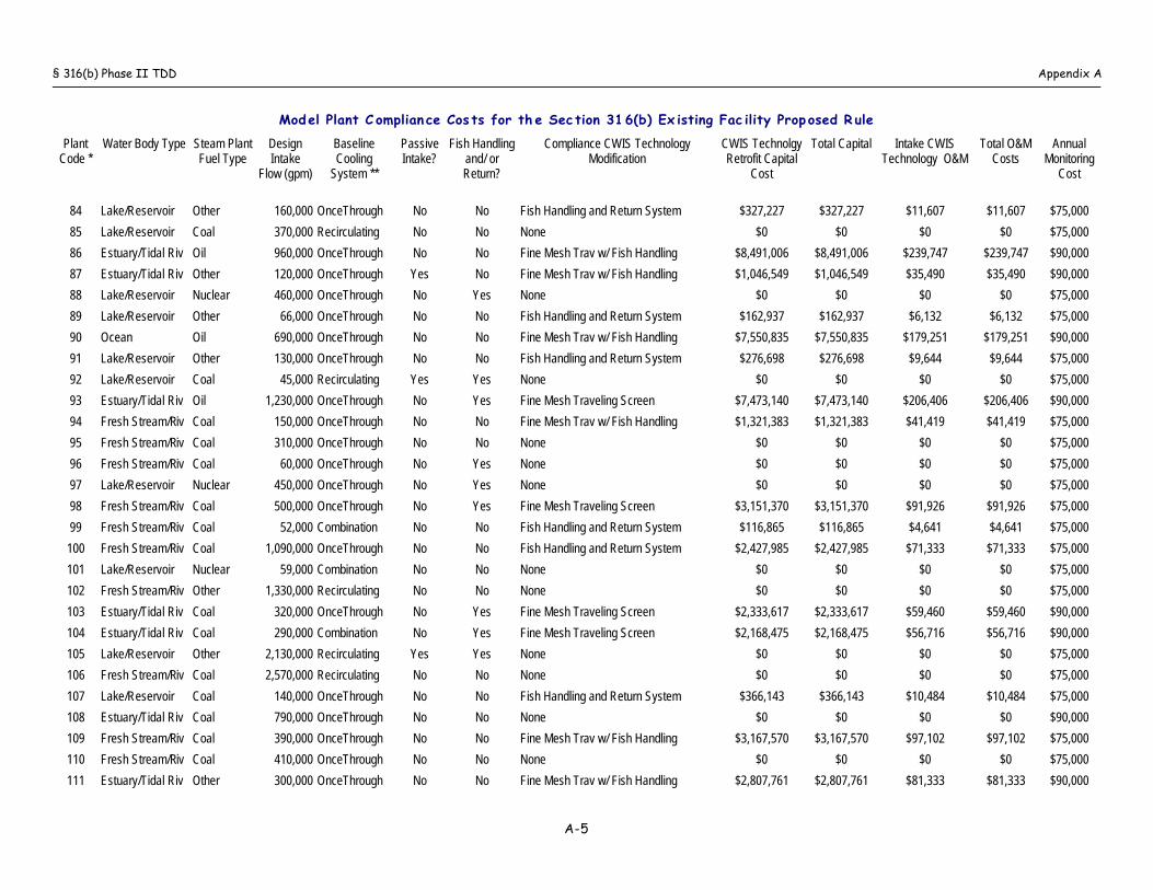
§ 316(b) Phase II TDD Appendix A
Model Plant C omplian ce Cos ts for th e Sec tion 316(b) Ex isting Fac ility Prop osed R ule
PlantCode *
Water Body Type Steam PlantFuel Type
DesignIntake
Flow (gpm)
BaselineCooling
System **
PassiveIntake?
Fish Handlingand/ orReturn?
Compliance CWIS TechnologyModification
CWIS TechnolgyRetrofit Capital
Cost
Total Capital Intake CWISTechnology O&M
Total O&MCosts
AnnualMonitoring
Cost
A-5
84 Lake/Reservoir Other 160,000 OnceThrough No No Fish Handling and Return System $327,227 $327,227 $11,607 $11,607 $75,000
85 Lake/Reservoir Coal 370,000 Recirculating No No None $0 $0 $0 $0 $75,000
86 Estuary/Tidal Riv Oil 960,000 OnceThrough No No Fine Mesh Trav w/ Fish Handling $8,491,006 $8,491,006 $239,747 $239,747 $90,000
87 Estuary/Tidal Riv Other 120,000 OnceThrough Yes No Fine Mesh Trav w/ Fish Handling $1,046,549 $1,046,549 $35,490 $35,490 $90,000
88 Lake/Reservoir Nuclear 460,000 OnceThrough No Yes None $0 $0 $0 $0 $75,000
89 Lake/Reservoir Other 66,000 OnceThrough No No Fish Handling and Return System $162,937 $162,937 $6,132 $6,132 $75,000
90 Ocean Oil 690,000 OnceThrough No No Fine Mesh Trav w/ Fish Handling $7,550,835 $7,550,835 $179,251 $179,251 $90,000
91 Lake/Reservoir Other 130,000 OnceThrough No No Fish Handling and Return System $276,698 $276,698 $9,644 $9,644 $75,000
92 Lake/Reservoir Coal 45,000 Recirculating Yes Yes None $0 $0 $0 $0 $75,000
93 Estuary/Tidal Riv Oil 1,230,000 OnceThrough No Yes Fine Mesh Traveling Screen $7,473,140 $7,473,140 $206,406 $206,406 $90,000
94 Fresh Stream/Riv Coal 150,000 OnceThrough No No Fine Mesh Trav w/ Fish Handling $1,321,383 $1,321,383 $41,419 $41,419 $75,000
95 Fresh Stream/Riv Coal 310,000 OnceThrough No No None $0 $0 $0 $0 $75,000
96 Fresh Stream/Riv Coal 60,000 OnceThrough No Yes None $0 $0 $0 $0 $75,000
97 Lake/Reservoir Nuclear 450,000 OnceThrough No Yes None $0 $0 $0 $0 $75,000
98 Fresh Stream/Riv Coal 500,000 OnceThrough No Yes Fine Mesh Traveling Screen $3,151,370 $3,151,370 $91,926 $91,926 $75,000
99 Fresh Stream/Riv Coal 52,000 Combination No No Fish Handling and Return System $116,865 $116,865 $4,641 $4,641 $75,000
100 Fresh Stream/Riv Coal 1,090,000 OnceThrough No No Fish Handling and Return System $2,427,985 $2,427,985 $71,333 $71,333 $75,000
101 Lake/Reservoir Nuclear 59,000 Combination No No None $0 $0 $0 $0 $75,000
102 Fresh Stream/Riv Other 1,330,000 Recirculating No No None $0 $0 $0 $0 $75,000
103 Estuary/Tidal Riv Coal 320,000 OnceThrough No Yes Fine Mesh Traveling Screen $2,333,617 $2,333,617 $59,460 $59,460 $90,000
104 Estuary/Tidal Riv Coal 290,000 Combination No Yes Fine Mesh Traveling Screen $2,168,475 $2,168,475 $56,716 $56,716 $90,000
105 Lake/Reservoir Other 2,130,000 Recirculating Yes Yes None $0 $0 $0 $0 $75,000
106 Fresh Stream/Riv Coal 2,570,000 Recirculating No No None $0 $0 $0 $0 $75,000
107 Lake/Reservoir Coal 140,000 OnceThrough No No Fish Handling and Return System $366,143 $366,143 $10,484 $10,484 $75,000
108 Estuary/Tidal Riv Coal 790,000 OnceThrough No No None $0 $0 $0 $0 $90,000
109 Fresh Stream/Riv Coal 390,000 OnceThrough No No Fine Mesh Trav w/ Fish Handling $3,167,570 $3,167,570 $97,102 $97,102 $75,000
110 Fresh Stream/Riv Coal 410,000 OnceThrough No No None $0 $0 $0 $0 $75,000
111 Estuary/Tidal Riv Other 300,000 OnceThrough No No Fine Mesh Trav w/ Fish Handling $2,807,761 $2,807,761 $81,333 $81,333 $90,000
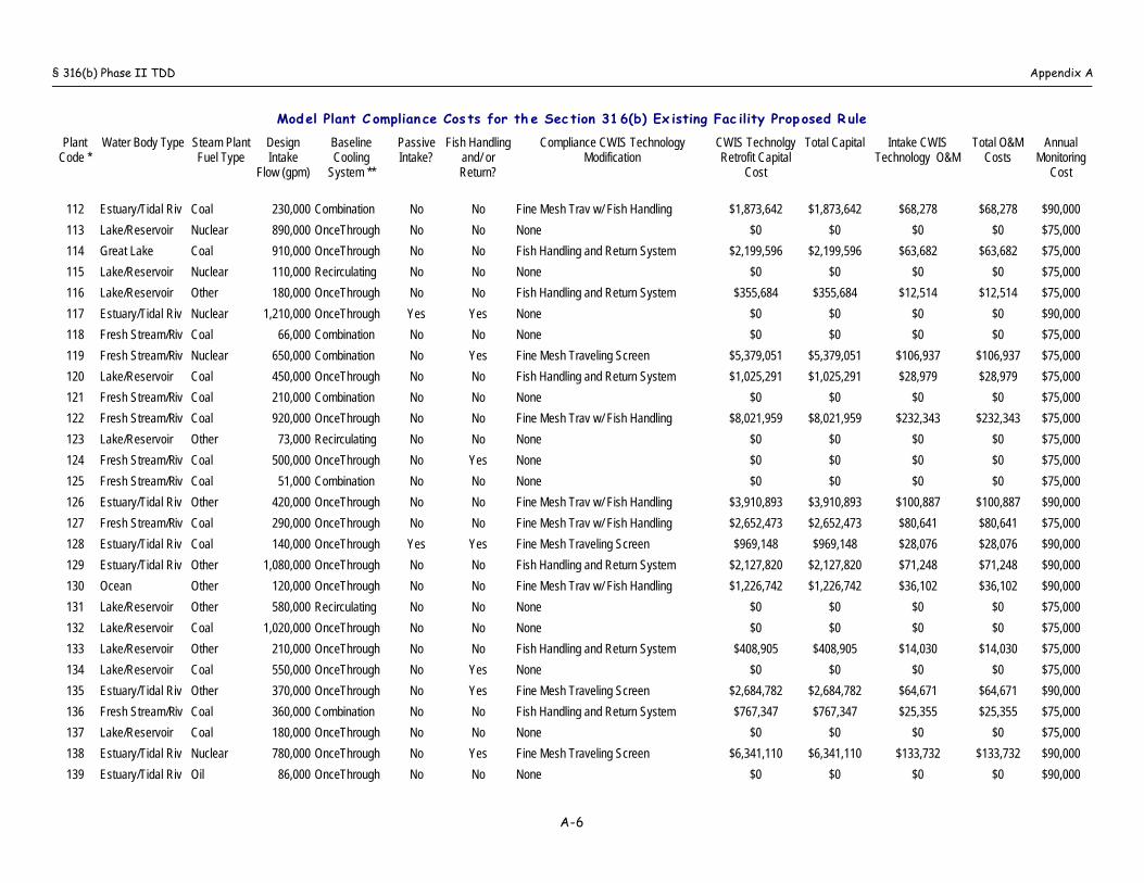
§ 316(b) Phase II TDD Appendix A
Model Plant C omplian ce Cos ts for th e Sec tion 316(b) Ex isting Fac ility Prop osed R ule
PlantCode *
Water Body Type Steam PlantFuel Type
DesignIntake
Flow (gpm)
BaselineCooling
System **
PassiveIntake?
Fish Handlingand/ orReturn?
Compliance CWIS TechnologyModification
CWIS TechnolgyRetrofit Capital
Cost
Total Capital Intake CWISTechnology O&M
Total O&MCosts
AnnualMonitoring
Cost
A-6
112 Estuary/Tidal Riv Coal 230,000 Combination No No Fine Mesh Trav w/ Fish Handling $1,873,642 $1,873,642 $68,278 $68,278 $90,000
113 Lake/Reservoir Nuclear 890,000 OnceThrough No No None $0 $0 $0 $0 $75,000
114 Great Lake Coal 910,000 OnceThrough No No Fish Handling and Return System $2,199,596 $2,199,596 $63,682 $63,682 $75,000
115 Lake/Reservoir Nuclear 110,000 Recirculating No No None $0 $0 $0 $0 $75,000
116 Lake/Reservoir Other 180,000 OnceThrough No No Fish Handling and Return System $355,684 $355,684 $12,514 $12,514 $75,000
117 Estuary/Tidal Riv Nuclear 1,210,000 OnceThrough Yes Yes None $0 $0 $0 $0 $90,000
118 Fresh Stream/Riv Coal 66,000 Combination No No None $0 $0 $0 $0 $75,000
119 Fresh Stream/Riv Nuclear 650,000 Combination No Yes Fine Mesh Traveling Screen $5,379,051 $5,379,051 $106,937 $106,937 $75,000
120 Lake/Reservoir Coal 450,000 OnceThrough No No Fish Handling and Return System $1,025,291 $1,025,291 $28,979 $28,979 $75,000
121 Fresh Stream/Riv Coal 210,000 Combination No No None $0 $0 $0 $0 $75,000
122 Fresh Stream/Riv Coal 920,000 OnceThrough No No Fine Mesh Trav w/ Fish Handling $8,021,959 $8,021,959 $232,343 $232,343 $75,000
123 Lake/Reservoir Other 73,000 Recirculating No No None $0 $0 $0 $0 $75,000
124 Fresh Stream/Riv Coal 500,000 OnceThrough No Yes None $0 $0 $0 $0 $75,000
125 Fresh Stream/Riv Coal 51,000 Combination No No None $0 $0 $0 $0 $75,000
126 Estuary/Tidal Riv Other 420,000 OnceThrough No No Fine Mesh Trav w/ Fish Handling $3,910,893 $3,910,893 $100,887 $100,887 $90,000
127 Fresh Stream/Riv Coal 290,000 OnceThrough No No Fine Mesh Trav w/ Fish Handling $2,652,473 $2,652,473 $80,641 $80,641 $75,000
128 Estuary/Tidal Riv Coal 140,000 OnceThrough Yes Yes Fine Mesh Traveling Screen $969,148 $969,148 $28,076 $28,076 $90,000
129 Estuary/Tidal Riv Other 1,080,000 OnceThrough No No Fish Handling and Return System $2,127,820 $2,127,820 $71,248 $71,248 $90,000
130 Ocean Other 120,000 OnceThrough No No Fine Mesh Trav w/ Fish Handling $1,226,742 $1,226,742 $36,102 $36,102 $90,000
131 Lake/Reservoir Other 580,000 Recirculating No No None $0 $0 $0 $0 $75,000
132 Lake/Reservoir Coal 1,020,000 OnceThrough No No None $0 $0 $0 $0 $75,000
133 Lake/Reservoir Other 210,000 OnceThrough No No Fish Handling and Return System $408,905 $408,905 $14,030 $14,030 $75,000
134 Lake/Reservoir Coal 550,000 OnceThrough No Yes None $0 $0 $0 $0 $75,000
135 Estuary/Tidal Riv Other 370,000 OnceThrough No Yes Fine Mesh Traveling Screen $2,684,782 $2,684,782 $64,671 $64,671 $90,000
136 Fresh Stream/Riv Coal 360,000 Combination No No Fish Handling and Return System $767,347 $767,347 $25,355 $25,355 $75,000
137 Lake/Reservoir Coal 180,000 OnceThrough No No None $0 $0 $0 $0 $75,000
138 Estuary/Tidal Riv Nuclear 780,000 OnceThrough No Yes Fine Mesh Traveling Screen $6,341,110 $6,341,110 $133,732 $133,732 $90,000
139 Estuary/Tidal Riv Oil 86,000 OnceThrough No No None $0 $0 $0 $0 $90,000
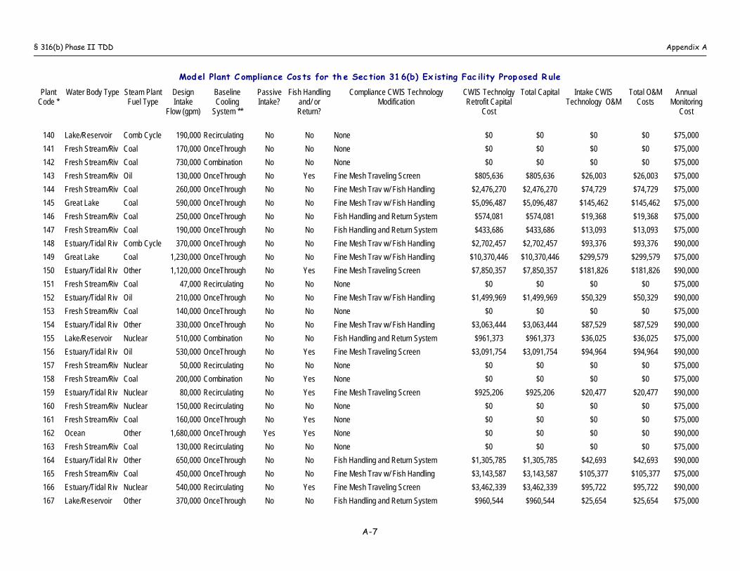
§ 316(b) Phase II TDD Appendix A
Model Plant C omplian ce Cos ts for th e Sec tion 316(b) Ex isting Fac ility Prop osed R ule
PlantCode *
Water Body Type Steam PlantFuel Type
DesignIntake
Flow (gpm)
BaselineCooling
System **
PassiveIntake?
Fish Handlingand/ orReturn?
Compliance CWIS TechnologyModification
CWIS TechnolgyRetrofit Capital
Cost
Total Capital Intake CWISTechnology O&M
Total O&MCosts
AnnualMonitoring
Cost
A-7
140 Lake/Reservoir Comb Cycle 190,000 Recirculating No No None $0 $0 $0 $0 $75,000
141 Fresh Stream/Riv Coal 170,000 OnceThrough No No None $0 $0 $0 $0 $75,000
142 Fresh Stream/Riv Coal 730,000 Combination No No None $0 $0 $0 $0 $75,000
143 Fresh Stream/Riv Oil 130,000 OnceThrough No Yes Fine Mesh Traveling Screen $805,636 $805,636 $26,003 $26,003 $75,000
144 Fresh Stream/Riv Coal 260,000 OnceThrough No No Fine Mesh Trav w/ Fish Handling $2,476,270 $2,476,270 $74,729 $74,729 $75,000
145 Great Lake Coal 590,000 OnceThrough No No Fine Mesh Trav w/ Fish Handling $5,096,487 $5,096,487 $145,462 $145,462 $75,000
146 Fresh Stream/Riv Coal 250,000 OnceThrough No No Fish Handling and Return System $574,081 $574,081 $19,368 $19,368 $75,000
147 Fresh Stream/Riv Coal 190,000 OnceThrough No No Fish Handling and Return System $433,686 $433,686 $13,093 $13,093 $75,000
148 Estuary/Tidal Riv Comb Cycle 370,000 OnceThrough No No Fine Mesh Trav w/ Fish Handling $2,702,457 $2,702,457 $93,376 $93,376 $90,000
149 Great Lake Coal 1,230,000 OnceThrough No No Fine Mesh Trav w/ Fish Handling $10,370,446 $10,370,446 $299,579 $299,579 $75,000
150 Estuary/Tidal Riv Other 1,120,000 OnceThrough No Yes Fine Mesh Traveling Screen $7,850,357 $7,850,357 $181,826 $181,826 $90,000
151 Fresh Stream/Riv Coal 47,000 Recirculating No No None $0 $0 $0 $0 $75,000
152 Estuary/Tidal Riv Oil 210,000 OnceThrough No No Fine Mesh Trav w/ Fish Handling $1,499,969 $1,499,969 $50,329 $50,329 $90,000
153 Fresh Stream/Riv Coal 140,000 OnceThrough No No None $0 $0 $0 $0 $75,000
154 Estuary/Tidal Riv Other 330,000 OnceThrough No No Fine Mesh Trav w/ Fish Handling $3,063,444 $3,063,444 $87,529 $87,529 $90,000
155 Lake/Reservoir Nuclear 510,000 Combination No No Fish Handling and Return System $961,373 $961,373 $36,025 $36,025 $75,000
156 Estuary/Tidal Riv Oil 530,000 OnceThrough No Yes Fine Mesh Traveling Screen $3,091,754 $3,091,754 $94,964 $94,964 $90,000
157 Fresh Stream/Riv Nuclear 50,000 Recirculating No No None $0 $0 $0 $0 $75,000
158 Fresh Stream/Riv Coal 200,000 Combination No Yes None $0 $0 $0 $0 $75,000
159 Estuary/Tidal Riv Nuclear 80,000 Recirculating No Yes Fine Mesh Traveling Screen $925,206 $925,206 $20,477 $20,477 $90,000
160 Fresh Stream/Riv Nuclear 150,000 Recirculating No No None $0 $0 $0 $0 $75,000
161 Fresh Stream/Riv Coal 160,000 OnceThrough No Yes None $0 $0 $0 $0 $75,000
162 Ocean Other 1,680,000 OnceThrough Yes Yes None $0 $0 $0 $0 $90,000
163 Fresh Stream/Riv Coal 130,000 Recirculating No No None $0 $0 $0 $0 $75,000
164 Estuary/Tidal Riv Other 650,000 OnceThrough No No Fish Handling and Return System $1,305,785 $1,305,785 $42,693 $42,693 $90,000
165 Fresh Stream/Riv Coal 450,000 OnceThrough No No Fine Mesh Trav w/ Fish Handling $3,143,587 $3,143,587 $105,377 $105,377 $75,000
166 Estuary/Tidal Riv Nuclear 540,000 Recirculating No Yes Fine Mesh Traveling Screen $3,462,339 $3,462,339 $95,722 $95,722 $90,000
167 Lake/Reservoir Other 370,000 OnceThrough No No Fish Handling and Return System $960,544 $960,544 $25,654 $25,654 $75,000
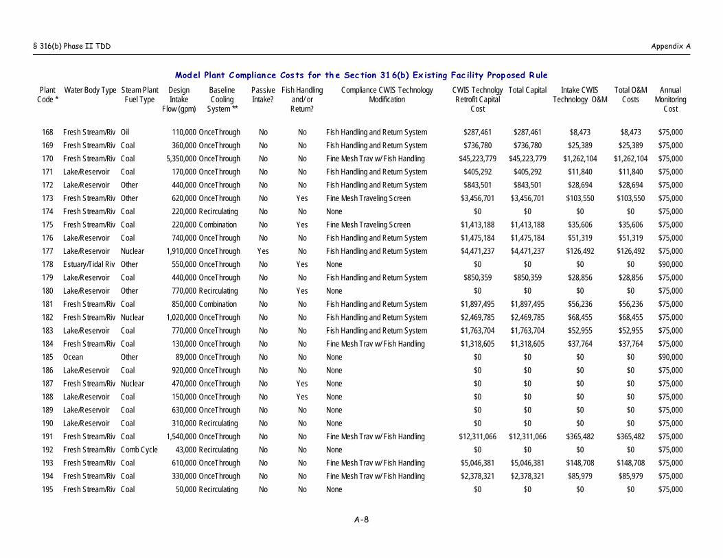
§ 316(b) Phase II TDD Appendix A
Model Plant C omplian ce Cos ts for th e Sec tion 316(b) Ex isting Fac ility Prop osed R ule
PlantCode *
Water Body Type Steam PlantFuel Type
DesignIntake
Flow (gpm)
BaselineCooling
System **
PassiveIntake?
Fish Handlingand/ orReturn?
Compliance CWIS TechnologyModification
CWIS TechnolgyRetrofit Capital
Cost
Total Capital Intake CWISTechnology O&M
Total O&MCosts
AnnualMonitoring
Cost
A-8
168 Fresh Stream/Riv Oil 110,000 OnceThrough No No Fish Handling and Return System $287,461 $287,461 $8,473 $8,473 $75,000
169 Fresh Stream/Riv Coal 360,000 OnceThrough No No Fish Handling and Return System $736,780 $736,780 $25,389 $25,389 $75,000
170 Fresh Stream/Riv Coal 5,350,000 OnceThrough No No Fine Mesh Trav w/ Fish Handling $45,223,779 $45,223,779 $1,262,104 $1,262,104 $75,000
171 Lake/Reservoir Coal 170,000 OnceThrough No No Fish Handling and Return System $405,292 $405,292 $11,840 $11,840 $75,000
172 Lake/Reservoir Other 440,000 OnceThrough No No Fish Handling and Return System $843,501 $843,501 $28,694 $28,694 $75,000
173 Fresh Stream/Riv Other 620,000 OnceThrough No Yes Fine Mesh Traveling Screen $3,456,701 $3,456,701 $103,550 $103,550 $75,000
174 Fresh Stream/Riv Coal 220,000 Recirculating No No None $0 $0 $0 $0 $75,000
175 Fresh Stream/Riv Coal 220,000 Combination No Yes Fine Mesh Traveling Screen $1,413,188 $1,413,188 $35,606 $35,606 $75,000
176 Lake/Reservoir Coal 740,000 OnceThrough No No Fish Handling and Return System $1,475,184 $1,475,184 $51,319 $51,319 $75,000
177 Lake/Reservoir Nuclear 1,910,000 OnceThrough Yes No Fish Handling and Return System $4,471,237 $4,471,237 $126,492 $126,492 $75,000
178 Estuary/Tidal Riv Other 550,000 OnceThrough No Yes None $0 $0 $0 $0 $90,000
179 Lake/Reservoir Coal 440,000 OnceThrough No No Fish Handling and Return System $850,359 $850,359 $28,856 $28,856 $75,000
180 Lake/Reservoir Other 770,000 Recirculating No Yes None $0 $0 $0 $0 $75,000
181 Fresh Stream/Riv Coal 850,000 Combination No No Fish Handling and Return System $1,897,495 $1,897,495 $56,236 $56,236 $75,000
182 Fresh Stream/Riv Nuclear 1,020,000 OnceThrough No No Fish Handling and Return System $2,469,785 $2,469,785 $68,455 $68,455 $75,000
183 Lake/Reservoir Coal 770,000 OnceThrough No No Fish Handling and Return System $1,763,704 $1,763,704 $52,955 $52,955 $75,000
184 Fresh Stream/Riv Coal 130,000 OnceThrough No No Fine Mesh Trav w/ Fish Handling $1,318,605 $1,318,605 $37,764 $37,764 $75,000
185 Ocean Other 89,000 OnceThrough No No None $0 $0 $0 $0 $90,000
186 Lake/Reservoir Coal 920,000 OnceThrough No No None $0 $0 $0 $0 $75,000
187 Fresh Stream/Riv Nuclear 470,000 OnceThrough No Yes None $0 $0 $0 $0 $75,000
188 Lake/Reservoir Coal 150,000 OnceThrough No Yes None $0 $0 $0 $0 $75,000
189 Lake/Reservoir Coal 630,000 OnceThrough No No None $0 $0 $0 $0 $75,000
190 Lake/Reservoir Coal 310,000 Recirculating No No None $0 $0 $0 $0 $75,000
191 Fresh Stream/Riv Coal 1,540,000 OnceThrough No No Fine Mesh Trav w/ Fish Handling $12,311,066 $12,311,066 $365,482 $365,482 $75,000
192 Fresh Stream/Riv Comb Cycle 43,000 Recirculating No No None $0 $0 $0 $0 $75,000
193 Fresh Stream/Riv Coal 610,000 OnceThrough No No Fine Mesh Trav w/ Fish Handling $5,046,381 $5,046,381 $148,708 $148,708 $75,000
194 Fresh Stream/Riv Coal 330,000 OnceThrough No No Fine Mesh Trav w/ Fish Handling $2,378,321 $2,378,321 $85,979 $85,979 $75,000
195 Fresh Stream/Riv Coal 50,000 Recirculating No No None $0 $0 $0 $0 $75,000
§ 316(b) Phase II TDD Appendix A
Model Plant C omplian ce Cos ts for th e Sec tion 316(b) Ex isting Fac ility Prop osed R ule
PlantCode *
Water Body Type Steam PlantFuel Type
DesignIntake
Flow (gpm)
BaselineCooling
System **
PassiveIntake?
Fish Handlingand/ orReturn?
Compliance CWIS TechnologyModification
CWIS TechnolgyRetrofit Capital
Cost
Total Capital Intake CWISTechnology O&M
Total O&MCosts
AnnualMonitoring
Cost
A-9
196 Lake/Reservoir Other 420,000 OnceThrough No No None $0 $0 $0 $0 $75,000
197 Fresh Stream/Riv Coal 170,000 OnceThrough No No Fish Handling and Return System $433,985 $433,985 $12,273 $12,273 $75,000
198 Lake/Reservoir Coal 550,000 Recirculating No Yes None $0 $0 $0 $0 $75,000
199 Lake/Reservoir Other 500,000 OnceThrough No No Fish Handling and Return System $1,017,517 $1,017,517 $35,981 $35,981 $75,000
200 Fresh Stream/Riv Coal 90,000 OnceThrough No No Fish Handling and Return System $209,422 $209,422 $7,499 $7,499 $75,000
201 Lake/Reservoir Coal 1,510,000 OnceThrough No No Fish Handling and Return System $2,915,937 $2,915,937 $99,551 $99,551 $75,000
202 Fresh Stream/Riv Coal 710,000 Combination No No Fine Mesh Trav w/ Fish Handling $6,000,929 $6,000,929 $182,006 $182,006 $75,000
203 Fresh Stream/Riv Coal 280,000 OnceThrough No No Fine Mesh Trav w/ Fish Handling $2,624,121 $2,624,121 $78,660 $78,660 $75,000
204 Estuary/Tidal Riv Nuclear 1,000,000 OnceThrough No Yes Fine Mesh Traveling Screen $8,707,797 $8,707,797 $169,706 $169,706 $90,000
205 Lake/Reservoir Nuclear 550,000 OnceThrough No No Fish Handling and Return System $1,018,849 $1,018,849 $38,532 $38,532 $75,000
206 Lake/Reservoir Nuclear 200,000 Combination No No None $0 $0 $0 $0 $75,000
207 Fresh Stream/Riv Coal 120,000 OnceThrough No Yes None $0 $0 $0 $0 $75,000
208 Lake/Reservoir Nuclear 1,130,000 OnceThrough No No Fish Handling and Return System $2,310,521 $2,310,521 $78,289 $78,289 $75,000
209 Fresh Stream/Riv Coal 230,000 OnceThrough No No Fine Mesh Trav w/ Fish Handling $2,192,914 $2,192,914 $69,478 $69,478 $75,000
210 Fresh Stream/Riv Coal 950,000 OnceThrough No No Fine Mesh Trav w/ Fish Handling $7,906,569 $7,906,569 $236,873 $236,873 $75,000
211 Fresh Stream/Riv Coal 420,000 Other No No None $0 $0 $0 $0 $75,000
212 Lake/Reservoir Other 76,000 OnceThrough No No None $0 $0 $0 $0 $75,000
213 Lake/Reservoir Comb Cycle 77,000 Combination No No None $0 $0 $0 $0 $75,000
214 Fresh Stream/Riv Coal 200,000 OnceThrough No No Fine Mesh Trav w/ Fish Handling $1,693,858 $1,693,858 $49,004 $49,004 $75,000
215 Lake/Reservoir Other 44,000 OnceThrough No No Fish Handling and Return System $102,577 $102,577 $4,165 $4,165 $75,000
216 Lake/Reservoir Coal 140,000 Recirculating No No None $0 $0 $0 $0 $75,000
217 Ocean Nuclear 560,000 OnceThrough Yes No None $0 $0 $0 $0 $90,000
218 Fresh Stream/Riv Coal 64,000 OnceThrough No No Fish Handling and Return System $147,805 $147,805 $6,027 $6,027 $75,000
219 Fresh Stream/Riv Coal 70,000 Recirculating No No None $0 $0 $0 $0 $75,000
220 Fresh Stream/Riv Other 260,000 Recirculating No No None $0 $0 $0 $0 $75,000
221 Lake/Reservoir Nuclear 79,000 Recirculating No No None $0 $0 $0 $0 $75,000
222 Fresh Stream/Riv Coal 160,000 OnceThrough No No Fish Handling and Return System $331,890 $331,890 $11,364 $11,364 $75,000
223 Fresh Stream/Riv Coal 88,000 Recirculating No No None $0 $0 $0 $0 $75,000
§ 316(b) Phase II TDD Appendix A
Model Plant C omplian ce Cos ts for th e Sec tion 316(b) Ex isting Fac ility Prop osed R ule
PlantCode *
Water Body Type Steam PlantFuel Type
DesignIntake
Flow (gpm)
BaselineCooling
System **
PassiveIntake?
Fish Handlingand/ orReturn?
Compliance CWIS TechnologyModification
CWIS TechnolgyRetrofit Capital
Cost
Total Capital Intake CWISTechnology O&M
Total O&MCosts
AnnualMonitoring
Cost
A-10
224 Lake/Reservoir Coal 820,000 OnceThrough No No Fish Handling and Return System $1,623,313 $1,623,313 $55,009 $55,009 $75,000
225 Ocean Other 170,000 OnceThrough Yes No Fish Handling and Return System $459,989 $459,989 $11,992 $11,992 $90,000
226 Estuary/Tidal Riv Oil 560,000 OnceThrough No No Fine Mesh Trav w/ Fish Handling $4,073,795 $4,073,795 $140,592 $140,592 $90,000
227 Estuary/Tidal Riv Other 230,000 OnceThrough No No None $0 $0 $0 $0 $90,000
228 Fresh Stream/Riv Coal 73,000 OnceThrough No No Fine Mesh Trav w/ Fish Handling $700,542 $700,542 $26,346 $26,346 $75,000
229 Fresh Stream/Riv Coal 260,000 Recirculating No No None $0 $0 $0 $0 $75,000
230 Estuary/Tidal Riv Other 1,280,000 OnceThrough No No Fish Handling and Return System $3,411,906 $3,411,906 $84,707 $84,707 $90,000
231 Ocean Nuclear 440,000 OnceThrough No Yes None $0 $0 $0 $0 $90,000
232 Lake/Reservoir Coal 71,000 OnceThrough No No None $0 $0 $0 $0 $75,000
233 Lake/Reservoir Oil 1,270,000 OnceThrough No No None $0 $0 $0 $0 $75,000
234 Estuary/Tidal Riv Other 290,000 OnceThrough No No Fish Handling and Return System $603,732 $603,732 $21,529 $21,529 $90,000
235 Fresh Stream/Riv Coal 850,000 OnceThrough No No Fine Mesh Trav w/ Fish Handling $7,316,195 $7,316,195 $204,078 $204,078 $75,000
236 Estuary/Tidal Riv Other 100,000 OnceThrough No No Fine Mesh Trav w/ Fish Handling $1,171,873 $1,171,873 $32,521 $32,521 $90,000
237 Fresh Stream/Riv Oil 660,000 OnceThrough No No None $0 $0 $0 $0 $75,000
238 Fresh Stream/Riv Coal 130,000 OnceThrough No Yes Fine Mesh Traveling Screen $913,055 $913,055 $26,501 $26,501 $75,000
239 Fresh Stream/Riv Coal 61,000 OnceThrough No No None $0 $0 $0 $0 $75,000
240 Fresh Stream/Riv Other 340,000 Recirculating No No None $0 $0 $0 $0 $75,000
241 Estuary/Tidal Riv Oil 2,680,000 OnceThrough No Yes Fine Mesh Traveling Screen $18,748,809 $18,748,809 $435,154 $435,154 $90,000
242 Lake/Reservoir Other 430,000 OnceThrough No No Fish Handling and Return System $825,540 $825,540 $28,255 $28,255 $75,000
243 Fresh Stream/Riv Nuclear 460,000 Other No No Fine Mesh Trav w/ Fish Handling $4,594,450 $4,594,450 $123,881 $123,881 $75,000
244 Fresh Stream/Riv Coal 340,000 OnceThrough No No Fine Mesh Trav w/ Fish Handling $2,239,456 $2,239,456 $88,464 $88,464 $75,000
245 Lake/Reservoir Coal 130,000 OnceThrough No No Fish Handling and Return System $342,708 $342,708 $10,077 $10,077 $75,000
246 Fresh Stream/Riv Coal 110,000 OnceThrough No No Fine Mesh Trav w/ Fish Handling $1,099,875 $1,099,875 $34,353 $34,353 $75,000
247 Lake/Reservoir Coal 480,000 Recirculating No No None $0 $0 $0 $0 $75,000
248 Estuary/Tidal Riv Other 580,000 OnceThrough No No Fish Handling and Return System $1,542,186 $1,542,186 $39,638 $39,638 $90,000
249 Great Lake Other 440,000 Combination Yes No Fine Mesh Trav w/ Fish Handling $3,666,639 $3,666,639 $104,091 $104,091 $75,000
250 Fresh Stream/Riv Coal 100,000 OnceThrough No No Fine Mesh Trav w/ Fish Handling $931,121 $931,121 $31,977 $31,977 $75,000
251 Lake/Reservoir Other 450,000 OnceThrough No No Fish Handling and Return System $929,538 $929,538 $33,096 $33,096 $75,000
§ 316(b) Phase II TDD Appendix A
Model Plant C omplian ce Cos ts for th e Sec tion 316(b) Ex isting Fac ility Prop osed R ule
PlantCode *
Water Body Type Steam PlantFuel Type
DesignIntake
Flow (gpm)
BaselineCooling
System **
PassiveIntake?
Fish Handlingand/ orReturn?
Compliance CWIS TechnologyModification
CWIS TechnolgyRetrofit Capital
Cost
Total Capital Intake CWISTechnology O&M
Total O&MCosts
AnnualMonitoring
Cost
A-11
252 Lake/Reservoir Coal 180,000 OnceThrough No No Fish Handling and Return System $373,886 $373,886 $12,393 $12,393 $75,000
253 Fresh Stream/Riv Coal 180,000 OnceThrough No No Fine Mesh Trav w/ Fish Handling $1,355,807 $1,355,807 $46,172 $46,172 $75,000
254 Lake/Reservoir Coal 74,000 OnceThrough No No Fish Handling and Return System $232,739 $232,739 $6,583 $6,583 $75,000
255 Fresh Stream/Riv Nuclear 630,000 Recirculating No No None $0 $0 $0 $0 $75,000
256 Fresh Stream/Riv Other 75,000 OnceThrough No No Fish Handling and Return System $188,492 $188,492 $6,631 $6,631 $75,000
257 Fresh Stream/Riv Other 1,070,000 Recirculating No No None $0 $0 $0 $0 $75,000
258 Fresh Stream/Riv Coal 430,000 OnceThrough No Yes None $0 $0 $0 $0 $75,000
259 Estuary/Tidal Riv Nuclear 110,000 OnceThrough No Yes Fine Mesh Traveling Screen $1,030,036 $1,030,036 $23,752 $23,752 $90,000
260 Lake/Reservoir Coal 1,050,000 Recirculating No No None $0 $0 $0 $0 $75,000
261 Fresh Stream/Riv Coal 140,000 OnceThrough No Yes None $0 $0 $0 $0 $75,000
262 Great Lake Coal 41,000 OnceThrough No No Fine Mesh Trav w/ Fish Handling $464,121 $464,121 $16,467 $16,467 $75,000
263 Fresh Stream/Riv Coal 88,000 Recirculating No No None $0 $0 $0 $0 $75,000
264 Lake/Reservoir Nuclear 5,440,000 OnceThrough No No Fish Handling and Return System $9,882,287 $9,882,287 $356,995 $356,995 $75,000
265 Fresh Stream/Riv Other 66,000 OnceThrough No No Fish Handling and Return System $217,718 $217,718 $6,137 $6,137 $75,000
266 Lake/Reservoir Coal 440,000 OnceThrough No No Fish Handling and Return System $858,875 $858,875 $28,905 $28,905 $75,000
267 Estuary/Tidal Riv Other 38,000 OnceThrough No No None $0 $0 $0 $0 $90,000
268 Estuary/Tidal Riv Coal 2,120,000 Combination No No Fine Mesh Trav w/ Fish Handling $15,282,924 $15,282,924 $509,611 $509,611 $90,000
269 Ocean Oil 360,000 OnceThrough No No Fine Mesh Trav w/ Fish Handling $3,851,922 $3,851,922 $91,062 $91,062 $90,000
270 Lake/Reservoir Coal 63,000 OnceThrough No No Fish Handling and Return System $161,118 $161,118 $5,985 $5,985 $75,000
271 Lake/Reservoir Coal 810,000 Recirculating No No None $0 $0 $0 $0 $75,000
272 Fresh Stream/Riv Coal 300,000 OnceThrough No No Fish Handling and Return System $749,245 $749,245 $22,251 $22,251 $75,000
273 Lake/Reservoir Other 320,000 OnceThrough No No Fish Handling and Return System $648,883 $648,883 $23,031 $23,031 $75,000
274 Fresh Stream/Riv Coal 45,000 OnceThrough No No None $0 $0 $0 $0 $75,000
275 Fresh Stream/Riv Coal 400,000 OnceThrough No No None $0 $0 $0 $0 $75,000
276 Fresh Stream/Riv Coal 240,000 OnceThrough No No Fine Mesh Trav w/ Fish Handling $1,926,190 $1,926,190 $70,751 $70,751 $75,000
277 Estuary/Tidal Riv Oil 220,000 OnceThrough No Yes Fine Mesh Traveling Screen $1,372,571 $1,372,571 $35,941 $35,941 $90,000
278 Fresh Stream/Riv Coal 120,000 OnceThrough No No Fish Handling and Return System $316,951 $316,951 $9,138 $9,138 $75,000
279 Fresh Stream/Riv Coal 80,000 OnceThrough No Yes None $0 $0 $0 $0 $75,000
§ 316(b) Phase II TDD Appendix A
Model Plant C omplian ce Cos ts for th e Sec tion 316(b) Ex isting Fac ility Prop osed R ule
PlantCode *
Water Body Type Steam PlantFuel Type
DesignIntake
Flow (gpm)
BaselineCooling
System **
PassiveIntake?
Fish Handlingand/ orReturn?
Compliance CWIS TechnologyModification
CWIS TechnolgyRetrofit Capital
Cost
Total Capital Intake CWISTechnology O&M
Total O&MCosts
AnnualMonitoring
Cost
A-12
280 Estuary/Tidal Riv Nuclear 2,020,000 OnceThrough No Yes Fine Mesh Traveling Screen $16,834,637 $16,834,637 $327,747 $327,747 $90,000
281 Lake/Reservoir Coal 370,000 OnceThrough No No Fish Handling and Return System $846,303 $846,303 $25,572 $25,572 $75,000
282 Lake/Reservoir Coal 700,000 OnceThrough No Yes None $0 $0 $0 $0 $75,000
283 Estuary/Tidal Riv Coal 390,000 OnceThrough No Yes Fine Mesh Traveling Screen $2,206,407 $2,206,407 $66,950 $66,950 $90,000
284 Fresh Stream/Riv Coal 230,000 OnceThrough No Yes None $0 $0 $0 $0 $75,000
285 Lake/Reservoir Coal 1,010,000 OnceThrough No No Fish Handling and Return System $1,992,079 $1,992,079 $68,370 $68,370 $75,000
286 Estuary/Tidal Riv Coal 1,500,000 OnceThrough No Yes None $0 $0 $0 $0 $90,000
287 Fresh Stream/Riv Coal 250,000 OnceThrough No No None $0 $0 $0 $0 $75,000
288 Estuary/Tidal Riv Oil 330,000 OnceThrough No No Fine Mesh Trav w/ Fish Handling $2,467,266 $2,467,266 $86,864 $86,864 $90,000
289 Fresh Stream/Riv Coal 590,000 OnceThrough No Yes None $0 $0 $0 $0 $75,000
290 Estuary/Tidal Riv Other 500,000 OnceThrough No No Fine Mesh Trav w/ Fish Handling $4,741,804 $4,741,804 $130,499 $130,499 $90,000
291 Fresh Stream/Riv Coal 120,000 Recirculating No No None $0 $0 $0 $0 $75,000
292 Lake/Reservoir Comb Cycle 72,000 OnceThrough No No None $0 $0 $0 $0 $75,000
293 Lake/Reservoir Other 720,000 Combination No No Fish Handling and Return System $1,432,577 $1,432,577 $50,358 $50,358 $75,000
294 Ocean Other 370,000 OnceThrough No No Fine Mesh Trav w/ Fish Handling $2,571,824 $2,571,824 $92,909 $92,909 $90,000
295 Fresh Stream/Riv Coal 180,000 OnceThrough No No Fish Handling and Return System $448,331 $448,331 $12,630 $12,630 $75,000
296 Estuary/Tidal Riv Other 100,000 OnceThrough No Yes None $0 $0 $0 $0 $90,000
297 Fresh Stream/Riv Other 510,000 OnceThrough No Yes None $0 $0 $0 $0 $75,000
298 Estuary/Tidal Riv Other 350,000 OnceThrough No No Fine Mesh Trav w/ Fish Handling $3,391,514 $3,391,514 $90,901 $90,901 $90,000
299 Fresh Stream/Riv Coal 39,000 Recirculating No No None $0 $0 $0 $0 $75,000
300 Estuary/Tidal Riv Comb Cycle 240,000 OnceThrough No Yes Fine Mesh Traveling Screen $1,957,099 $1,957,099 $50,798 $50,798 $90,000
301 Estuary/Tidal Riv Coal 440,000 OnceThrough No No Fine Mesh Trav w/ Fish Handling $4,016,929 $4,016,929 $103,736 $103,736 $90,000
302 Fresh Stream/Riv Other 910,000 OnceThrough No No None $0 $0 $0 $0 $75,000
303 Fresh Stream/Riv Nuclear 61,000 Recirculating No No None $0 $0 $0 $0 $75,000
304 Fresh Stream/Riv Coal 490,000 OnceThrough No No None $0 $0 $0 $0 $75,000
305 Lake/Reservoir Coal 250,000 OnceThrough No Yes None $0 $0 $0 $0 $75,000
306 Estuary/Tidal Riv Other 140,000 OnceThrough No No None $0 $0 $0 $0 $90,000
307 Estuary/Tidal Riv Oil 230,000 Combination No Yes None $0 $0 $0 $0 $90,000
§ 316(b) Phase II TDD Appendix A
Model Plant C omplian ce Cos ts for th e Sec tion 316(b) Ex isting Fac ility Prop osed R ule
PlantCode *
Water Body Type Steam PlantFuel Type
DesignIntake
Flow (gpm)
BaselineCooling
System **
PassiveIntake?
Fish Handlingand/ orReturn?
Compliance CWIS TechnologyModification
CWIS TechnolgyRetrofit Capital
Cost
Total Capital Intake CWISTechnology O&M
Total O&MCosts
AnnualMonitoring
Cost
A-13
308 Fresh Stream/Riv Oil 180,000 OnceThrough No No Fish Handling and Return System $435,199 $435,199 $12,499 $12,499 $75,000
309 Lake/Reservoir Other 660,000 OnceThrough No No Fish Handling and Return System $1,273,883 $1,273,883 $43,246 $43,246 $75,000
310 Lake/Reservoir Other 100,000 Recirculating No No None $0 $0 $0 $0 $75,000
311 Fresh Stream/Riv Coal 130,000 OnceThrough No No Fish Handling and Return System $287,270 $287,270 $10,113 $10,113 $75,000
312 Fresh Stream/Riv Other 83,000 OnceThrough No No Fish Handling and Return System $190,035 $190,035 $7,113 $7,113 $75,000
313 Fresh Stream/Riv Other 190,000 OnceThrough No No Fish Handling and Return System $468,083 $468,083 $13,300 $13,300 $75,000
314 Fresh Stream/Riv Coal 950,000 OnceThrough No No Fine Mesh Trav w/ Fish Handling $7,825,161 $7,825,161 $237,278 $237,278 $75,000
315 Fresh Stream/Riv Coal 270,000 OnceThrough No No Fish Handling and Return System $699,405 $699,405 $20,414 $20,414 $75,000
316 Lake/Reservoir Nuclear 380,000 OnceThrough Yes Yes None $0 $0 $0 $0 $75,000
317 Fresh Stream/Riv Other 180,000 OnceThrough No Yes None $0 $0 $0 $0 $75,000
318 Lake/Reservoir Other 280,000 OnceThrough No No Fish Handling and Return System $589,745 $589,745 $21,056 $21,056 $75,000
319 Fresh Stream/Riv Coal 360,000 Other No No Fine Mesh Trav w/ Fish Handling $2,332,769 $2,332,769 $91,387 $91,387 $75,000
320 Lake/Reservoir Coal 1,010,000 OnceThrough No No Fish Handling and Return System $1,859,551 $1,859,551 $68,197 $68,197 $75,000
321 Lake/Reservoir Comb Cycle 150,000 OnceThrough No No Fish Handling and Return System $326,129 $326,129 $11,118 $11,118 $75,000
322 Fresh Stream/Riv Coal 520,000 OnceThrough No Yes Fine Mesh Traveling Screen $3,364,264 $3,364,264 $93,702 $93,702 $75,000
323 Lake/Reservoir Coal 650,000 OnceThrough No No Fish Handling and Return System $1,558,441 $1,558,441 $42,662 $42,662 $75,000
324 Fresh Stream/Riv Coal 70,000 OnceThrough No No Fish Handling and Return System $201,299 $201,299 $6,356 $6,356 $75,000
325 Fresh Stream/Riv Nuclear 870,000 OnceThrough No No Fine Mesh Trav w/ Fish Handling $8,084,704 $8,084,704 $206,638 $206,638 $75,000
326 Fresh Stream/Riv Nuclear 76,000 Recirculating No No None $0 $0 $0 $0 $75,000
327 Estuary/Tidal Riv Oil 2,400,000 OnceThrough No No Fish Handling and Return System $6,379,540 $6,379,540 $157,514 $157,514 $90,000
328 Estuary/Tidal Riv Coal 82,000 OnceThrough No No None $0 $0 $0 $0 $90,000
329 Fresh Stream/Riv Coal 1,370,000 OnceThrough No Yes Fine Mesh Traveling Screen $9,113,298 $9,113,298 $234,978 $234,978 $75,000
330 Fresh Stream/Riv Coal 110,000 OnceThrough No No Fine Mesh Trav w/ Fish Handling $1,065,898 $1,065,898 $34,257 $34,257 $75,000
331 Lake/Reservoir Coal 440,000 Recirculating No No None $0 $0 $0 $0 $75,000
332 Great Lake Coal 310,000 OnceThrough No No Fine Mesh Trav w/ Fish Handling $2,587,410 $2,587,410 $82,934 $82,934 $75,000
333 Estuary/Tidal Riv Coal 130,000 OnceThrough No Yes Fine Mesh Traveling Screen $1,068,066 $1,068,066 $26,804 $26,804 $90,000
334 Fresh Stream/Riv Other 320,000 OnceThrough No Yes None $0 $0 $0 $0 $75,000
335 Fresh Stream/Riv Coal 1,080,000 OnceThrough No No Fine Mesh Trav w/ Fish Handling $7,564,068 $7,564,068 $257,171 $257,171 $75,000
§ 316(b) Phase II TDD Appendix A
Model Plant C omplian ce Cos ts for th e Sec tion 316(b) Ex isting Fac ility Prop osed R ule
PlantCode *
Water Body Type Steam PlantFuel Type
DesignIntake
Flow (gpm)
BaselineCooling
System **
PassiveIntake?
Fish Handlingand/ orReturn?
Compliance CWIS TechnologyModification
CWIS TechnolgyRetrofit Capital
Cost
Total Capital Intake CWISTechnology O&M
Total O&MCosts
AnnualMonitoring
Cost
A-14
336 Fresh Stream/Riv Coal 690,000 Combination No No Fine Mesh Trav w/ Fish Handling $4,962,647 $4,962,647 $178,383 $178,383 $75,000
337 Fresh Stream/Riv Coal 1,050,000 OnceThrough No No Fish Handling and Return System $2,157,319 $2,157,319 $69,773 $69,773 $75,000
338 Fresh Stream/Riv Coal 200,000 Combination No No Fine Mesh Trav w/ Fish Handling $1,373,019 $1,373,019 $49,203 $49,203 $75,000
339 Fresh Stream/Riv Nuclear 360,000 Combination No Yes None $0 $0 $0 $0 $75,000
340 Fresh Stream/Riv Coal 700,000 OnceThrough No Yes Fine Mesh Traveling Screen $4,545,063 $4,545,063 $125,850 $125,850 $75,000
341 Fresh Stream/Riv Coal 100,000 Combination No Yes None $0 $0 $0 $0 $75,000
342 Fresh Stream/Riv Coal 310,000 Recirculating No Yes None $0 $0 $0 $0 $75,000
343 Lake/Reservoir Coal 42,000 Recirculating No No None $0 $0 $0 $0 $75,000
344 Fresh Stream/Riv Coal 110,000 Recirculating No No None $0 $0 $0 $0 $75,000
345 Fresh Stream/Riv Other 1,050,000 OnceThrough No Yes None $0 $0 $0 $0 $75,000
346 Estuary/Tidal Riv Other 1,050,000 OnceThrough No Yes None $0 $0 $0 $0 $90,000
347 Lake/Reservoir Nuclear 810,000 Combination Yes No Fish Handling and Return System $1,542,486 $1,542,486 $54,459 $54,459 $75,000
348 Fresh Stream/Riv Coal 150,000 OnceThrough No Yes None $0 $0 $0 $0 $75,000
349 Fresh Stream/Riv Coal 190,000 OnceThrough No No Fish Handling and Return System $396,969 $396,969 $13,144 $13,144 $75,000
350 Lake/Reservoir Coal 130,000 OnceThrough No No Fish Handling and Return System $292,561 $292,561 $10,031 $10,031 $75,000
351 Estuary/Tidal Riv Comb Cycle 65,000 OnceThrough No No None $0 $0 $0 $0 $90,000
352 Fresh Stream/Riv Coal 820,000 Combination No Yes Fine Mesh Traveling Screen $4,601,345 $4,601,345 $137,922 $137,922 $75,000
353 Ocean Other 420,000 OnceThrough Yes No Fine Mesh Trav w/ Fish Handling $3,939,024 $3,939,024 $101,372 $101,372 $90,000
354 Fresh Stream/Riv Other 130,000 OnceThrough No No Fine Mesh Trav w/ Fish Handling $985,436 $985,436 $36,506 $36,506 $75,000
355 Fresh Stream/Riv Coal 270,000 OnceThrough No No Fine Mesh Trav w/ Fish Handling $2,420,874 $2,420,874 $76,748 $76,748 $75,000
356 Fresh Stream/Riv Coal 70,000 OnceThrough No No Fine Mesh Trav w/ Fish Handling $771,245 $771,245 $25,669 $25,669 $75,000
357 Fresh Stream/Riv Coal 200,000 OnceThrough No Yes None $0 $0 $0 $0 $75,000
358 Estuary/Tidal Riv Coal 1,710,000 OnceThrough No No Fine Mesh Trav w/ Fish Handling $12,330,972 $12,330,972 $409,972 $409,972 $90,000
359 Estuary/Tidal Riv Other 140,000 OnceThrough No Yes None $0 $0 $0 $0 $90,000
360 Fresh Stream/Riv Nuclear 67,000 OnceThrough No No Fish Handling and Return System $171,556 $171,556 $6,200 $6,200 $75,000
361 Fresh Stream/Riv Coal 500,000 OnceThrough No No Fine Mesh Trav w/ Fish Handling $3,572,845 $3,572,845 $130,325 $130,325 $75,000
362 Lake/Reservoir Coal 390,000 OnceThrough No No Fish Handling and Return System $766,332 $766,332 $26,664 $26,664 $75,000
363 Estuary/Tidal Riv Other 65,000 OnceThrough No No Fine Mesh Trav w/ Fish Handling $639,845 $639,845 $24,760 $24,760 $90,000
§ 316(b) Phase II TDD Appendix A
Model Plant C omplian ce Cos ts for th e Sec tion 316(b) Ex isting Fac ility Prop osed R ule
PlantCode *
Water Body Type Steam PlantFuel Type
DesignIntake
Flow (gpm)
BaselineCooling
System **
PassiveIntake?
Fish Handlingand/ orReturn?
Compliance CWIS TechnologyModification
CWIS TechnolgyRetrofit Capital
Cost
Total Capital Intake CWISTechnology O&M
Total O&MCosts
AnnualMonitoring
Cost
A-15
364 Lake/Reservoir Comb Cycle 130,000 OnceThrough No No Fish Handling and Return System $274,030 $274,030 $9,819 $9,819 $75,000
365 Fresh Stream/Riv Other 830,000 Recirculating No No None $0 $0 $0 $0 $75,000
366 Fresh Stream/Riv Coal 190,000 OnceThrough No No Fish Handling and Return System $396,532 $396,532 $13,041 $13,041 $75,000
367 Fresh Stream/Riv Coal 87,000 OnceThrough Yes No Fine Mesh Trav w/ Fish Handling $693,184 $693,184 $29,089 $29,089 $75,000
368 Ocean Nuclear 1,030,000 OnceThrough Yes No Fine Mesh Trav w/ Fish Handling $8,182,772 $8,182,772 $249,720 $249,720 $90,000
369 Lake/Reservoir Coal 400,000 OnceThrough No No Fish Handling and Return System $973,966 $973,966 $27,075 $27,075 $75,000
370 Fresh Stream/Riv Coal 550,000 OnceThrough No No Fish Handling and Return System $1,314,223 $1,314,223 $38,449 $38,449 $75,000
371 Fresh Stream/Riv Coal 270,000 OnceThrough No No Fish Handling and Return System $738,387 $738,387 $20,134 $20,134 $75,000
372 Fresh Stream/Riv Other 39,000 OnceThrough No Yes None $0 $0 $0 $0 $75,000
373 Fresh Stream/Riv Coal 340,000 OnceThrough No No Fine Mesh Trav w/ Fish Handling $3,019,394 $3,019,394 $88,587 $88,587 $75,000
374 Estuary/Tidal Riv Coal 210,000 Combination Yes No Fine Mesh Trav w/ Fish Handling $1,373,170 $1,373,170 $51,369 $51,369 $90,000
375 Fresh Stream/Riv Coal 42,000 Recirculating No No None $0 $0 $0 $0 $75,000
376 Lake/Reservoir Coal 170,000 OnceThrough No No Fish Handling and Return System $405,704 $405,704 $12,323 $12,323 $75,000
377 Fresh Stream/Riv Nuclear 140,000 Recirculating No No None $0 $0 $0 $0 $75,000
378 Fresh Stream/Riv Coal 67,000 OnceThrough No No Fish Handling and Return System $175,112 $175,112 $6,189 $6,189 $75,000
379 Fresh Stream/Riv Coal 450,000 OnceThrough No No None $0 $0 $0 $0 $75,000
380 Fresh Stream/Riv Other 91,000 OnceThrough No Yes None $0 $0 $0 $0 $75,000
381 Fresh Stream/Riv Comb Cycle 120,000 Combination No Yes None $0 $0 $0 $0 $75,000
382 Lake/Reservoir Coal 500,000 OnceThrough No Yes None $0 $0 $0 $0 $75,000
383 Fresh Stream/Riv Coal 97,000 OnceThrough No No Fish Handling and Return System $261,841 $261,841 $7,930 $7,930 $75,000
384 Fresh Stream/Riv Coal 300,000 Combination No No Fine Mesh Trav w/ Fish Handling $2,607,043 $2,607,043 $80,990 $80,990 $75,000
385 Fresh Stream/Riv Oil 110,000 OnceThrough No No Fish Handling and Return System $301,754 $301,754 $8,961 $8,961 $75,000
386 Fresh Stream/Riv Coal 780,000 OnceThrough No No Fine Mesh Trav w/ Fish Handling $5,533,505 $5,533,505 $193,850 $193,850 $75,000
387 Fresh Stream/Riv Coal 370,000 OnceThrough No No None $0 $0 $0 $0 $75,000
388 Fresh Stream/Riv Nuclear 1,180,000 OnceThrough No No None $0 $0 $0 $0 $75,000
389 Fresh Stream/Riv Coal 74,000 OnceThrough No Yes None $0 $0 $0 $0 $75,000
390 Estuary/Tidal Riv Other 380,000 OnceThrough No No Fish Handling and Return System $842,401 $842,401 $26,320 $26,320 $90,000
391 Fresh Stream/Riv Coal 240,000 OnceThrough No No Fine Mesh Trav w/ Fish Handling $2,262,696 $2,262,696 $70,725 $70,725 $75,000
§ 316(b) Phase II TDD Appendix A
Model Plant C omplian ce Cos ts for th e Sec tion 316(b) Ex isting Fac ility Prop osed R ule
PlantCode *
Water Body Type Steam PlantFuel Type
DesignIntake
Flow (gpm)
BaselineCooling
System **
PassiveIntake?
Fish Handlingand/ orReturn?
Compliance CWIS TechnologyModification
CWIS TechnolgyRetrofit Capital
Cost
Total Capital Intake CWISTechnology O&M
Total O&MCosts
AnnualMonitoring
Cost
A-16
392 Fresh Stream/Riv Coal 1,030,000 OnceThrough No No Fish Handling and Return System $2,402,438 $2,402,438 $69,117 $69,117 $75,000
393 Estuary/Tidal Riv Other 520,000 OnceThrough Yes No Fine Mesh Trav w/ Fish Handling $4,708,410 $4,708,410 $133,910 $133,910 $90,000
394 Fresh Stream/Riv Coal 54,000 OnceThrough No No None $0 $0 $0 $0 $75,000
395 Estuary/Tidal Riv Other 2,100,000 OnceThrough No Yes Fine Mesh Traveling Screen $14,707,137 $14,707,137 $349,761 $349,761 $90,000
396 Lake/Reservoir Coal 200,000 OnceThrough No No None $0 $0 $0 $0 $75,000
397 Great Lake Coal 170,000 OnceThrough No No Fish Handling and Return System $411,092 $411,092 $12,118 $12,118 $75,000
398 Fresh Stream/Riv Coal 180,000 OnceThrough No No Fish Handling and Return System $327,604 $327,604 $12,448 $12,448 $75,000
399 Fresh Stream/Riv Coal 190,000 Other No Yes Fine Mesh Traveling Screen $1,006,660 $1,006,660 $33,417 $33,417 $75,000
400 Great Lake Coal 840,000 OnceThrough Yes No Fine Mesh Trav w/ Fish Handling $6,968,299 $6,968,299 $202,908 $202,908 $75,000
401 Fresh Stream/Riv Coal 620,000 OnceThrough No Yes None $0 $0 $0 $0 $75,000
402 Estuary/Tidal Riv Oil 570,000 OnceThrough No Yes Fine Mesh Traveling Screen $3,279,537 $3,279,537 $98,996 $98,996 $90,000
403 Fresh Stream/Riv Coal 280,000 OnceThrough No No Fine Mesh Trav w/ Fish Handling $2,494,743 $2,494,743 $77,936 $77,936 $75,000
404 Lake/Reservoir Coal 1,120,000 OnceThrough No No Fish Handling and Return System $2,163,010 $2,163,010 $72,624 $72,624 $75,000
405 Fresh Stream/Riv Coal 480,000 OnceThrough No No Fish Handling and Return System $1,153,848 $1,153,848 $34,608 $34,608 $75,000
406 Estuary/Tidal Riv Coal 310,000 Combination No Yes None $0 $0 $0 $0 $90,000
407 Fresh Stream/Riv Other 300,000 OnceThrough No No Fish Handling and Return System $628,979 $628,979 $21,986 $21,986 $75,000
408 Lake/Reservoir Nuclear 83,000 Recirculating No No None $0 $0 $0 $0 $75,000
409 Fresh Stream/Riv Coal 1,000,000 OnceThrough No No Fish Handling and Return System $2,254,314 $2,254,314 $67,586 $67,586 $75,000
410 Fresh Stream/Riv Other 89,000 OnceThrough No No None $0 $0 $0 $0 $75,000
411 Estuary/Tidal Riv Other 95,000 OnceThrough No No Fine Mesh Trav w/ Fish Handling $829,916 $829,916 $30,663 $30,663 $90,000
412 Lake/Reservoir Nuclear 2,200,000 OnceThrough No No Fish Handling and Return System $4,230,547 $4,230,547 $143,782 $143,782 $75,000
413 Fresh Stream/Riv Coal 1,900,000 OnceThrough No No Fine Mesh Trav w/ Fish Handling $13,190,121 $13,190,121 $456,702 $456,702 $75,000
414 Fresh Stream/Riv Other 350,000 Recirculating No Yes None $0 $0 $0 $0 $75,000
415 Ocean Oil 1,990,000 OnceThrough No No Fine Mesh Trav w/ Fish Handling $14,339,794 $14,339,794 $471,062 $471,062 $90,000
416 Lake/Reservoir Other 160,000 OnceThrough No No Fish Handling and Return System $333,612 $333,612 $11,814 $11,814 $75,000
417 Lake/Reservoir Coal 610,000 Recirculating No Yes None $0 $0 $0 $0 $75,000
418 Lake/Reservoir Other 650,000 OnceThrough No No Fish Handling and Return System $1,248,502 $1,248,502 $42,636 $42,636 $75,000
419 Estuary/Tidal Riv Other 1,200,000 OnceThrough No Yes Fine Mesh Traveling Screen $6,563,060 $6,563,060 $203,833 $203,833 $90,000
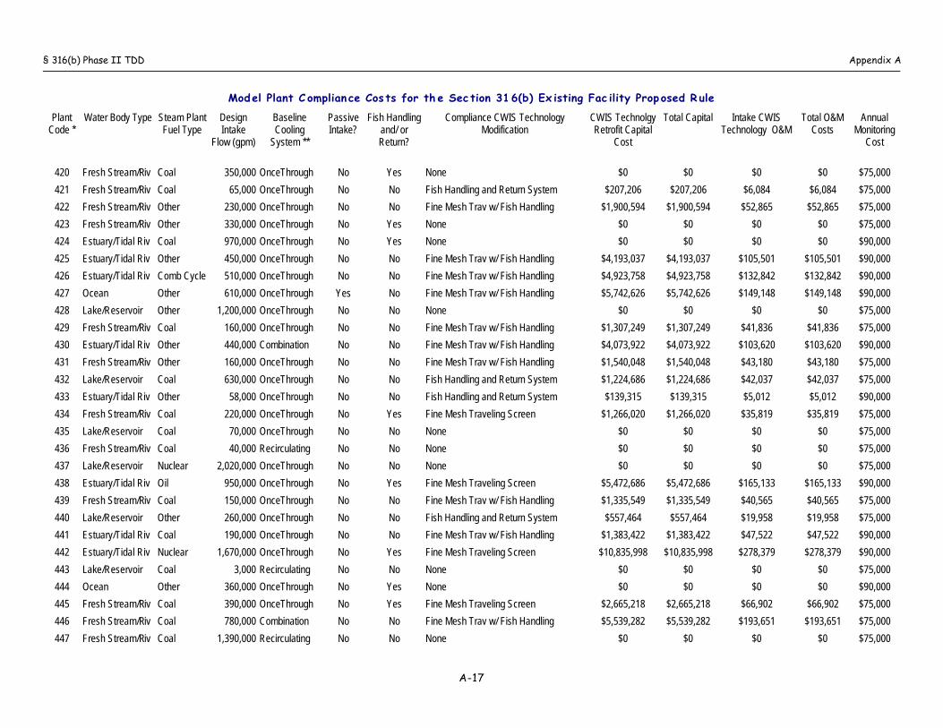
§ 316(b) Phase II TDD Appendix A
Model Plant C omplian ce Cos ts for th e Sec tion 316(b) Ex isting Fac ility Prop osed R ule
PlantCode *
Water Body Type Steam PlantFuel Type
DesignIntake
Flow (gpm)
BaselineCooling
System **
PassiveIntake?
Fish Handlingand/ orReturn?
Compliance CWIS TechnologyModification
CWIS TechnolgyRetrofit Capital
Cost
Total Capital Intake CWISTechnology O&M
Total O&MCosts
AnnualMonitoring
Cost
A-17
420 Fresh Stream/Riv Coal 350,000 OnceThrough No Yes None $0 $0 $0 $0 $75,000
421 Fresh Stream/Riv Coal 65,000 OnceThrough No No Fish Handling and Return System $207,206 $207,206 $6,084 $6,084 $75,000
422 Fresh Stream/Riv Other 230,000 OnceThrough No No Fine Mesh Trav w/ Fish Handling $1,900,594 $1,900,594 $52,865 $52,865 $75,000
423 Fresh Stream/Riv Other 330,000 OnceThrough No Yes None $0 $0 $0 $0 $75,000
424 Estuary/Tidal Riv Coal 970,000 OnceThrough No Yes None $0 $0 $0 $0 $90,000
425 Estuary/Tidal Riv Other 450,000 OnceThrough No No Fine Mesh Trav w/ Fish Handling $4,193,037 $4,193,037 $105,501 $105,501 $90,000
426 Estuary/Tidal Riv Comb Cycle 510,000 OnceThrough No No Fine Mesh Trav w/ Fish Handling $4,923,758 $4,923,758 $132,842 $132,842 $90,000
427 Ocean Other 610,000 OnceThrough Yes No Fine Mesh Trav w/ Fish Handling $5,742,626 $5,742,626 $149,148 $149,148 $90,000
428 Lake/Reservoir Other 1,200,000 OnceThrough No No None $0 $0 $0 $0 $75,000
429 Fresh Stream/Riv Coal 160,000 OnceThrough No No Fine Mesh Trav w/ Fish Handling $1,307,249 $1,307,249 $41,836 $41,836 $75,000
430 Estuary/Tidal Riv Other 440,000 Combination No No Fine Mesh Trav w/ Fish Handling $4,073,922 $4,073,922 $103,620 $103,620 $90,000
431 Fresh Stream/Riv Other 160,000 OnceThrough No No Fine Mesh Trav w/ Fish Handling $1,540,048 $1,540,048 $43,180 $43,180 $75,000
432 Lake/Reservoir Coal 630,000 OnceThrough No No Fish Handling and Return System $1,224,686 $1,224,686 $42,037 $42,037 $75,000
433 Estuary/Tidal Riv Other 58,000 OnceThrough No No Fish Handling and Return System $139,315 $139,315 $5,012 $5,012 $90,000
434 Fresh Stream/Riv Coal 220,000 OnceThrough No Yes Fine Mesh Traveling Screen $1,266,020 $1,266,020 $35,819 $35,819 $75,000
435 Lake/Reservoir Coal 70,000 OnceThrough No No None $0 $0 $0 $0 $75,000
436 Fresh Stream/Riv Coal 40,000 Recirculating No No None $0 $0 $0 $0 $75,000
437 Lake/Reservoir Nuclear 2,020,000 OnceThrough No No None $0 $0 $0 $0 $75,000
438 Estuary/Tidal Riv Oil 950,000 OnceThrough No Yes Fine Mesh Traveling Screen $5,472,686 $5,472,686 $165,133 $165,133 $90,000
439 Fresh Stream/Riv Coal 150,000 OnceThrough No No Fine Mesh Trav w/ Fish Handling $1,335,549 $1,335,549 $40,565 $40,565 $75,000
440 Lake/Reservoir Other 260,000 OnceThrough No No Fish Handling and Return System $557,464 $557,464 $19,958 $19,958 $75,000
441 Estuary/Tidal Riv Coal 190,000 OnceThrough No No Fine Mesh Trav w/ Fish Handling $1,383,422 $1,383,422 $47,522 $47,522 $90,000
442 Estuary/Tidal Riv Nuclear 1,670,000 OnceThrough No Yes Fine Mesh Traveling Screen $10,835,998 $10,835,998 $278,379 $278,379 $90,000
443 Lake/Reservoir Coal 3,000 Recirculating No No None $0 $0 $0 $0 $75,000
444 Ocean Other 360,000 OnceThrough No Yes None $0 $0 $0 $0 $90,000
445 Fresh Stream/Riv Coal 390,000 OnceThrough No Yes Fine Mesh Traveling Screen $2,665,218 $2,665,218 $66,902 $66,902 $75,000
446 Fresh Stream/Riv Coal 780,000 Combination No No Fine Mesh Trav w/ Fish Handling $5,539,282 $5,539,282 $193,651 $193,651 $75,000
447 Fresh Stream/Riv Coal 1,390,000 Recirculating No No None $0 $0 $0 $0 $75,000
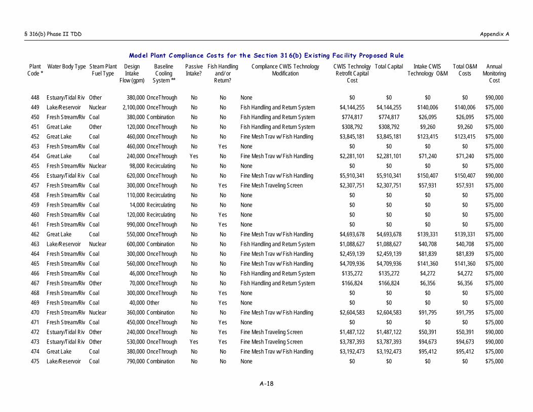
§ 316(b) Phase II TDD Appendix A
Model Plant C omplian ce Cos ts for th e Sec tion 316(b) Ex isting Fac ility Prop osed R ule
PlantCode *
Water Body Type Steam PlantFuel Type
DesignIntake
Flow (gpm)
BaselineCooling
System **
PassiveIntake?
Fish Handlingand/ orReturn?
Compliance CWIS TechnologyModification
CWIS TechnolgyRetrofit Capital
Cost
Total Capital Intake CWISTechnology O&M
Total O&MCosts
AnnualMonitoring
Cost
A-18
448 Estuary/Tidal Riv Other 380,000 OnceThrough No No None $0 $0 $0 $0 $90,000
449 Lake/Reservoir Nuclear 2,100,000 OnceThrough No No Fish Handling and Return System $4,144,255 $4,144,255 $140,006 $140,006 $75,000
450 Fresh Stream/Riv Coal 380,000 Combination No No Fish Handling and Return System $774,817 $774,817 $26,095 $26,095 $75,000
451 Great Lake Other 120,000 OnceThrough No No Fish Handling and Return System $308,792 $308,792 $9,260 $9,260 $75,000
452 Great Lake Coal 460,000 OnceThrough No No Fine Mesh Trav w/ Fish Handling $3,845,181 $3,845,181 $123,415 $123,415 $75,000
453 Fresh Stream/Riv Coal 460,000 OnceThrough No Yes None $0 $0 $0 $0 $75,000
454 Great Lake Coal 240,000 OnceThrough Yes No Fine Mesh Trav w/ Fish Handling $2,281,101 $2,281,101 $71,240 $71,240 $75,000
455 Fresh Stream/Riv Nuclear 98,000 Recirculating No No None $0 $0 $0 $0 $75,000
456 Estuary/Tidal Riv Coal 620,000 OnceThrough No No Fine Mesh Trav w/ Fish Handling $5,910,341 $5,910,341 $150,407 $150,407 $90,000
457 Fresh Stream/Riv Coal 300,000 OnceThrough No Yes Fine Mesh Traveling Screen $2,307,751 $2,307,751 $57,931 $57,931 $75,000
458 Fresh Stream/Riv Coal 110,000 Recirculating No No None $0 $0 $0 $0 $75,000
459 Fresh Stream/Riv Coal 14,000 Recirculating No No None $0 $0 $0 $0 $75,000
460 Fresh Stream/Riv Coal 120,000 Recirculating No Yes None $0 $0 $0 $0 $75,000
461 Fresh Stream/Riv Coal 990,000 OnceThrough No Yes None $0 $0 $0 $0 $75,000
462 Great Lake Coal 550,000 OnceThrough No No Fine Mesh Trav w/ Fish Handling $4,693,678 $4,693,678 $139,331 $139,331 $75,000
463 Lake/Reservoir Nuclear 600,000 Combination No No Fish Handling and Return System $1,088,627 $1,088,627 $40,708 $40,708 $75,000
464 Fresh Stream/Riv Coal 300,000 OnceThrough No No Fine Mesh Trav w/ Fish Handling $2,459,139 $2,459,139 $81,839 $81,839 $75,000
465 Fresh Stream/Riv Coal 560,000 OnceThrough No No Fine Mesh Trav w/ Fish Handling $4,709,936 $4,709,936 $141,360 $141,360 $75,000
466 Fresh Stream/Riv Coal 46,000 OnceThrough No No Fish Handling and Return System $135,272 $135,272 $4,272 $4,272 $75,000
467 Fresh Stream/Riv Other 70,000 OnceThrough No No Fish Handling and Return System $166,824 $166,824 $6,356 $6,356 $75,000
468 Fresh Stream/Riv Coal 300,000 OnceThrough No Yes None $0 $0 $0 $0 $75,000
469 Fresh Stream/Riv Coal 40,000 Other No Yes None $0 $0 $0 $0 $75,000
470 Fresh Stream/Riv Nuclear 360,000 Combination No No Fine Mesh Trav w/ Fish Handling $2,604,583 $2,604,583 $91,795 $91,795 $75,000
471 Fresh Stream/Riv Coal 450,000 OnceThrough No Yes None $0 $0 $0 $0 $75,000
472 Estuary/Tidal Riv Other 240,000 OnceThrough No Yes Fine Mesh Traveling Screen $1,487,122 $1,487,122 $50,391 $50,391 $90,000
473 Estuary/Tidal Riv Other 530,000 OnceThrough Yes Yes Fine Mesh Traveling Screen $3,787,393 $3,787,393 $94,673 $94,673 $90,000
474 Great Lake Coal 380,000 OnceThrough No No Fine Mesh Trav w/ Fish Handling $3,192,473 $3,192,473 $95,412 $95,412 $75,000
475 Lake/Reservoir Coal 790,000 Combination No No None $0 $0 $0 $0 $75,000
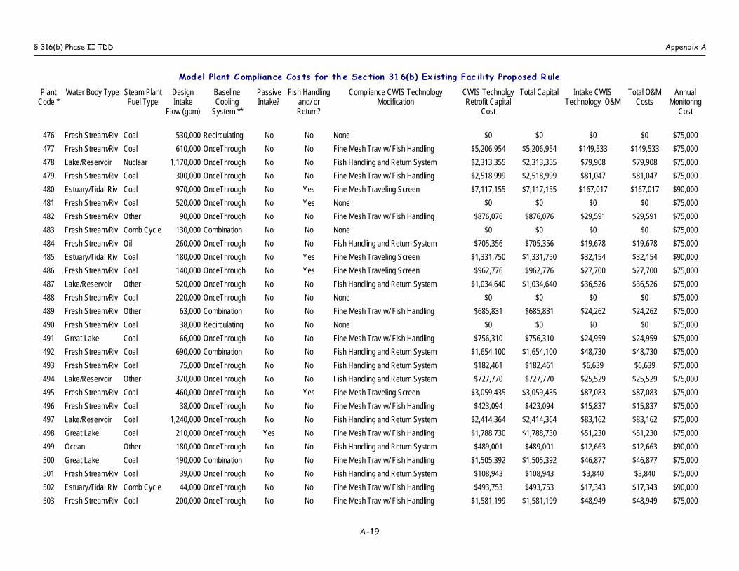
§ 316(b) Phase II TDD Appendix A
Model Plant C omplian ce Cos ts for th e Sec tion 316(b) Ex isting Fac ility Prop osed R ule
PlantCode *
Water Body Type Steam PlantFuel Type
DesignIntake
Flow (gpm)
BaselineCooling
System **
PassiveIntake?
Fish Handlingand/ orReturn?
Compliance CWIS TechnologyModification
CWIS TechnolgyRetrofit Capital
Cost
Total Capital Intake CWISTechnology O&M
Total O&MCosts
AnnualMonitoring
Cost
A-19
476 Fresh Stream/Riv Coal 530,000 Recirculating No No None $0 $0 $0 $0 $75,000
477 Fresh Stream/Riv Coal 610,000 OnceThrough No No Fine Mesh Trav w/ Fish Handling $5,206,954 $5,206,954 $149,533 $149,533 $75,000
478 Lake/Reservoir Nuclear 1,170,000 OnceThrough No No Fish Handling and Return System $2,313,355 $2,313,355 $79,908 $79,908 $75,000
479 Fresh Stream/Riv Coal 300,000 OnceThrough No No Fine Mesh Trav w/ Fish Handling $2,518,999 $2,518,999 $81,047 $81,047 $75,000
480 Estuary/Tidal Riv Coal 970,000 OnceThrough No Yes Fine Mesh Traveling Screen $7,117,155 $7,117,155 $167,017 $167,017 $90,000
481 Fresh Stream/Riv Coal 520,000 OnceThrough No Yes None $0 $0 $0 $0 $75,000
482 Fresh Stream/Riv Other 90,000 OnceThrough No No Fine Mesh Trav w/ Fish Handling $876,076 $876,076 $29,591 $29,591 $75,000
483 Fresh Stream/Riv Comb Cycle 130,000 Combination No No None $0 $0 $0 $0 $75,000
484 Fresh Stream/Riv Oil 260,000 OnceThrough No No Fish Handling and Return System $705,356 $705,356 $19,678 $19,678 $75,000
485 Estuary/Tidal Riv Coal 180,000 OnceThrough No Yes Fine Mesh Traveling Screen $1,331,750 $1,331,750 $32,154 $32,154 $90,000
486 Fresh Stream/Riv Coal 140,000 OnceThrough No Yes Fine Mesh Traveling Screen $962,776 $962,776 $27,700 $27,700 $75,000
487 Lake/Reservoir Other 520,000 OnceThrough No No Fish Handling and Return System $1,034,640 $1,034,640 $36,526 $36,526 $75,000
488 Fresh Stream/Riv Coal 220,000 OnceThrough No No None $0 $0 $0 $0 $75,000
489 Fresh Stream/Riv Other 63,000 Combination No No Fine Mesh Trav w/ Fish Handling $685,831 $685,831 $24,262 $24,262 $75,000
490 Fresh Stream/Riv Coal 38,000 Recirculating No No None $0 $0 $0 $0 $75,000
491 Great Lake Coal 66,000 OnceThrough No No Fine Mesh Trav w/ Fish Handling $756,310 $756,310 $24,959 $24,959 $75,000
492 Fresh Stream/Riv Coal 690,000 Combination No No Fish Handling and Return System $1,654,100 $1,654,100 $48,730 $48,730 $75,000
493 Fresh Stream/Riv Coal 75,000 OnceThrough No No Fish Handling and Return System $182,461 $182,461 $6,639 $6,639 $75,000
494 Lake/Reservoir Other 370,000 OnceThrough No No Fish Handling and Return System $727,770 $727,770 $25,529 $25,529 $75,000
495 Fresh Stream/Riv Coal 460,000 OnceThrough No Yes Fine Mesh Traveling Screen $3,059,435 $3,059,435 $87,083 $87,083 $75,000
496 Fresh Stream/Riv Coal 38,000 OnceThrough No No Fine Mesh Trav w/ Fish Handling $423,094 $423,094 $15,837 $15,837 $75,000
497 Lake/Reservoir Coal 1,240,000 OnceThrough No No Fish Handling and Return System $2,414,364 $2,414,364 $83,162 $83,162 $75,000
498 Great Lake Coal 210,000 OnceThrough Yes No Fine Mesh Trav w/ Fish Handling $1,788,730 $1,788,730 $51,230 $51,230 $75,000
499 Ocean Other 180,000 OnceThrough No No Fish Handling and Return System $489,001 $489,001 $12,663 $12,663 $90,000
500 Great Lake Coal 190,000 Combination No No Fine Mesh Trav w/ Fish Handling $1,505,392 $1,505,392 $46,877 $46,877 $75,000
501 Fresh Stream/Riv Coal 39,000 OnceThrough No No Fish Handling and Return System $108,943 $108,943 $3,840 $3,840 $75,000
502 Estuary/Tidal Riv Comb Cycle 44,000 OnceThrough No No Fine Mesh Trav w/ Fish Handling $493,753 $493,753 $17,343 $17,343 $90,000
503 Fresh Stream/Riv Coal 200,000 OnceThrough No No Fine Mesh Trav w/ Fish Handling $1,581,199 $1,581,199 $48,949 $48,949 $75,000
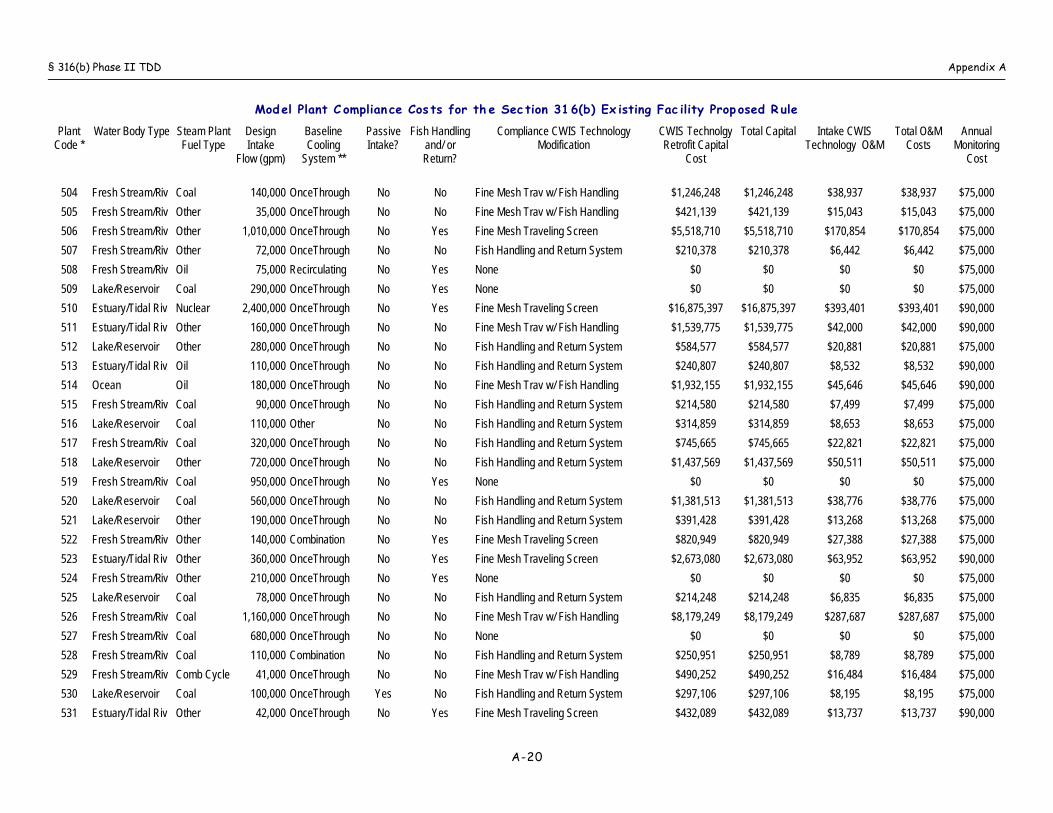
§ 316(b) Phase II TDD Appendix A
Model Plant C omplian ce Cos ts for th e Sec tion 316(b) Ex isting Fac ility Prop osed R ule
PlantCode *
Water Body Type Steam PlantFuel Type
DesignIntake
Flow (gpm)
BaselineCooling
System **
PassiveIntake?
Fish Handlingand/ orReturn?
Compliance CWIS TechnologyModification
CWIS TechnolgyRetrofit Capital
Cost
Total Capital Intake CWISTechnology O&M
Total O&MCosts
AnnualMonitoring
Cost
A-20
504 Fresh Stream/Riv Coal 140,000 OnceThrough No No Fine Mesh Trav w/ Fish Handling $1,246,248 $1,246,248 $38,937 $38,937 $75,000
505 Fresh Stream/Riv Other 35,000 OnceThrough No No Fine Mesh Trav w/ Fish Handling $421,139 $421,139 $15,043 $15,043 $75,000
506 Fresh Stream/Riv Other 1,010,000 OnceThrough No Yes Fine Mesh Traveling Screen $5,518,710 $5,518,710 $170,854 $170,854 $75,000
507 Fresh Stream/Riv Other 72,000 OnceThrough No No Fish Handling and Return System $210,378 $210,378 $6,442 $6,442 $75,000
508 Fresh Stream/Riv Oil 75,000 Recirculating No Yes None $0 $0 $0 $0 $75,000
509 Lake/Reservoir Coal 290,000 OnceThrough No Yes None $0 $0 $0 $0 $75,000
510 Estuary/Tidal Riv Nuclear 2,400,000 OnceThrough No Yes Fine Mesh Traveling Screen $16,875,397 $16,875,397 $393,401 $393,401 $90,000
511 Estuary/Tidal Riv Other 160,000 OnceThrough No No Fine Mesh Trav w/ Fish Handling $1,539,775 $1,539,775 $42,000 $42,000 $90,000
512 Lake/Reservoir Other 280,000 OnceThrough No No Fish Handling and Return System $584,577 $584,577 $20,881 $20,881 $75,000
513 Estuary/Tidal Riv Oil 110,000 OnceThrough No No Fish Handling and Return System $240,807 $240,807 $8,532 $8,532 $90,000
514 Ocean Oil 180,000 OnceThrough No No Fine Mesh Trav w/ Fish Handling $1,932,155 $1,932,155 $45,646 $45,646 $90,000
515 Fresh Stream/Riv Coal 90,000 OnceThrough No No Fish Handling and Return System $214,580 $214,580 $7,499 $7,499 $75,000
516 Lake/Reservoir Coal 110,000 Other No No Fish Handling and Return System $314,859 $314,859 $8,653 $8,653 $75,000
517 Fresh Stream/Riv Coal 320,000 OnceThrough No No Fish Handling and Return System $745,665 $745,665 $22,821 $22,821 $75,000
518 Lake/Reservoir Other 720,000 OnceThrough No No Fish Handling and Return System $1,437,569 $1,437,569 $50,511 $50,511 $75,000
519 Fresh Stream/Riv Coal 950,000 OnceThrough No Yes None $0 $0 $0 $0 $75,000
520 Lake/Reservoir Coal 560,000 OnceThrough No No Fish Handling and Return System $1,381,513 $1,381,513 $38,776 $38,776 $75,000
521 Lake/Reservoir Other 190,000 OnceThrough No No Fish Handling and Return System $391,428 $391,428 $13,268 $13,268 $75,000
522 Fresh Stream/Riv Other 140,000 Combination No Yes Fine Mesh Traveling Screen $820,949 $820,949 $27,388 $27,388 $75,000
523 Estuary/Tidal Riv Other 360,000 OnceThrough No Yes Fine Mesh Traveling Screen $2,673,080 $2,673,080 $63,952 $63,952 $90,000
524 Fresh Stream/Riv Other 210,000 OnceThrough No Yes None $0 $0 $0 $0 $75,000
525 Lake/Reservoir Coal 78,000 OnceThrough No No Fish Handling and Return System $214,248 $214,248 $6,835 $6,835 $75,000
526 Fresh Stream/Riv Coal 1,160,000 OnceThrough No No Fine Mesh Trav w/ Fish Handling $8,179,249 $8,179,249 $287,687 $287,687 $75,000
527 Fresh Stream/Riv Coal 680,000 OnceThrough No No None $0 $0 $0 $0 $75,000
528 Fresh Stream/Riv Coal 110,000 Combination No No Fish Handling and Return System $250,951 $250,951 $8,789 $8,789 $75,000
529 Fresh Stream/Riv Comb Cycle 41,000 OnceThrough No No Fine Mesh Trav w/ Fish Handling $490,252 $490,252 $16,484 $16,484 $75,000
530 Lake/Reservoir Coal 100,000 OnceThrough Yes No Fish Handling and Return System $297,106 $297,106 $8,195 $8,195 $75,000
531 Estuary/Tidal Riv Other 42,000 OnceThrough No Yes Fine Mesh Traveling Screen $432,089 $432,089 $13,737 $13,737 $90,000
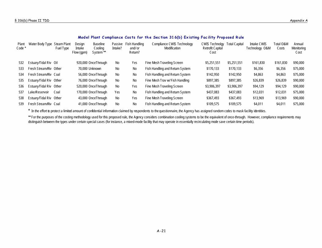
§ 316(b) Phase II TDD Appendix A
Model Plant C omplian ce Cos ts for th e Sec tion 316(b) Ex isting Fac ility Prop osed R ule
PlantCode *
Water Body Type Steam PlantFuel Type
DesignIntake
Flow (gpm)
BaselineCooling
System **
PassiveIntake?
Fish Handlingand/ orReturn?
Compliance CWIS TechnologyModification
CWIS TechnolgyRetrofit Capital
Cost
Total Capital Intake CWISTechnology O&M
Total O&MCosts
AnnualMonitoring
Cost
A-21
532 Estuary/Tidal Riv Oil 920,000 OnceThrough No Yes Fine Mesh Traveling Screen $5,251,551 $5,251,551 $161,830 $161,830 $90,000
533 Fresh Stream/Riv Other 70,000 Unknown No No Fish Handling and Return System $170,133 $170,133 $6,356 $6,356 $75,000
534 Fresh Stream/Riv Coal 56,000 OnceThrough No No Fish Handling and Return System $142,950 $142,950 $4,863 $4,863 $75,000
535 Estuary/Tidal Riv Other 76,000 OnceThrough No No Fine Mesh Trav w/ Fish Handling $897,385 $897,385 $26,839 $26,839 $90,000
536 Estuary/Tidal Riv Other 520,000 OnceThrough No Yes Fine Mesh Traveling Screen $3,906,397 $3,906,397 $94,129 $94,129 $90,000
537 Lake/Reservoir Coal 170,000 OnceThrough Yes No Fish Handling and Return System $437,083 $437,083 $12,031 $12,031 $75,000
538 Estuary/Tidal Riv Other 43,000 OnceThrough No Yes Fine Mesh Traveling Screen $367,493 $367,493 $13,969 $13,969 $90,000
539 Fresh Stream/Riv Coal 41,000 OnceThrough No No Fish Handling and Return System $109,575 $109,575 $4,011 $4,011 $75,000
* In the effort to protect a limited amount of confidential information claimed by respondents to the questionnaire, the Agency has assigned random codes to mask facility identities.
** For the purposes of the costing methodology used for this proposed rule, the Agency considers combination cooling systems to be the equivalent of once-through. However, compliance requirements may
distinguish between the types under certain special cases (for instance, a mixed-mode facility that may operate in essentially recirculating mode save certain time periods).

§ 316(b) Phase II TDD Appendix A
A-22
THIS PAGE INTENTIONALLY LEFT BLANK

§ 316(b) Phase II TDD Technology Cost Curves
Appendix B: Technology Cost Curves
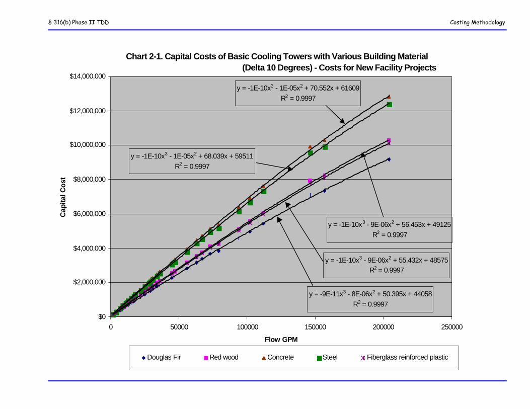
§ 316(b) Phase II TDD Costing Methodology
Chart 2-1. Capital Costs of Basic Cooling Towers with Various Building Material (Delta 10 Degrees) - Costs for New Facility Projects
y = -9E-11x3 - 8E-06x2 + 50.395x + 44058R2 = 0.9997
y = -1E-10x3 - 9E-06x2 + 55.432x + 48575R2 = 0.9997
y = -1E-10x3 - 9E-06x2 + 56.453x + 49125R2 = 0.9997
y = -1E-10x3 - 1E-05x2 + 68.039x + 59511R2 = 0.9997
y = -1E-10x3 - 1E-05x2 + 70.552x + 61609R2 = 0.9997
$0
$2,000,000
$4,000,000
$6,000,000
$8,000,000
$10,000,000
$12,000,000
$14,000,000
0 50000 100000 150000 200000 250000
Flow GPM
Cap
ital C
ost
Douglas Fir Red wood Concrete Steel Fiberglass reinforced plastic
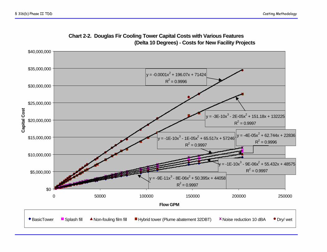
§ 316(b) Phase II TDD Costing Methodology
Chart 2-2. Douglas Fir Cooling Tower Capital Costs with Various Features (Delta 10 Degrees) - Costs for New Facility Projects
y = -0.0001x2 + 196.07x + 71424
R2 = 0.9996
y = -3E-10x3 - 2E-05x2 + 151.18x + 132225
R2 = 0.9997
y = -1E-10x3 - 1E-05x2 + 65.517x + 57246
R2 = 0.9997
y = -4E-05x2 + 62.744x + 22836
R2 = 0.9996
y = -1E-10x3 - 9E-06x2 + 55.432x + 48575
R2 = 0.9997
y = -9E-11x3 - 8E-06x2 + 50.395x + 44058
R2 = 0.9997$0
$5,000,000
$10,000,000
$15,000,000
$20,000,000
$25,000,000
$30,000,000
$35,000,000
$40,000,000
0 50000 100000 150000 200000 250000
Flow GPM
Cap
ital C
ost
BasicTower Splash fill Non-fouling film fill Hybrid tower (Plume abatement 32DBT) Noise reduction 10 dBA Dry/ wet
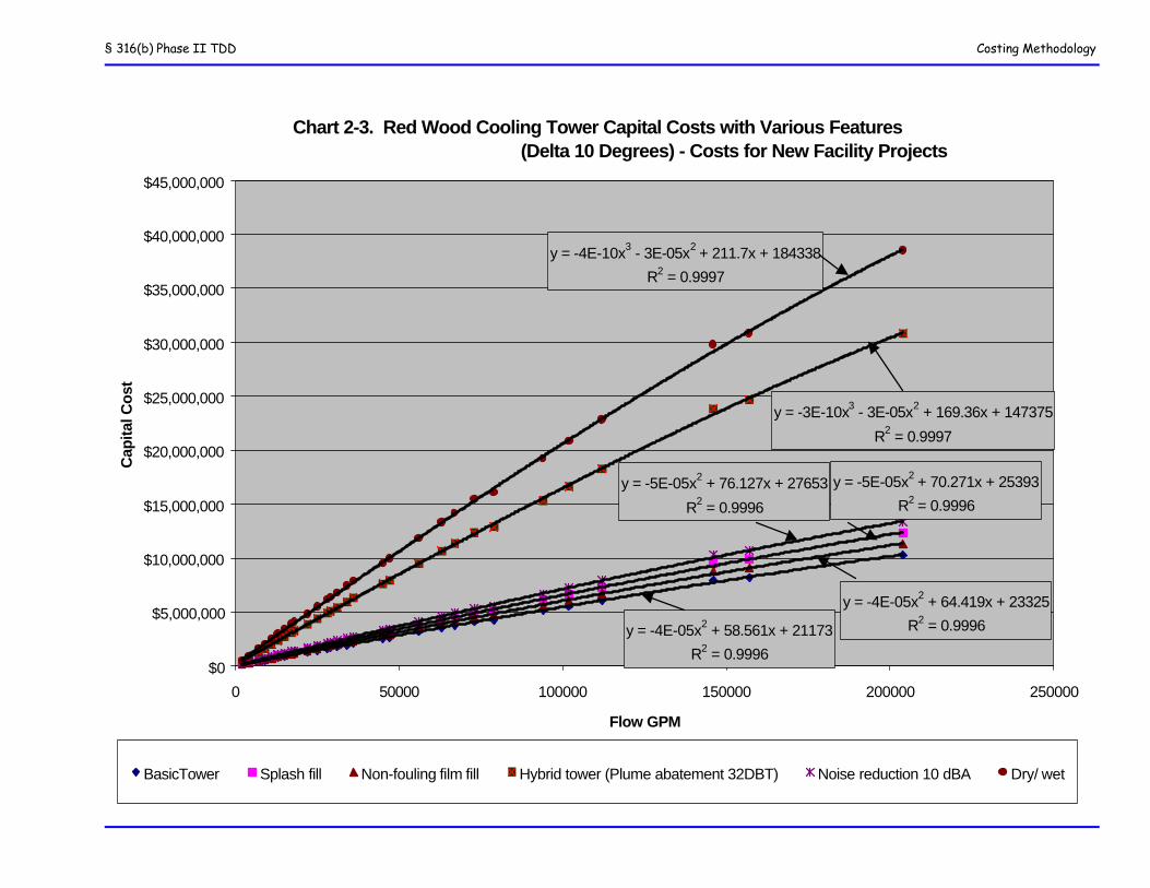
§ 316(b) Phase II TDD Costing Methodology
Chart 2-3. Red Wood Cooling Tower Capital Costs with Various Features (Delta 10 Degrees) - Costs for New Facility Projects
y = -4E-10x3 - 3E-05x2 + 211.7x + 184338
R2 = 0.9997
y = -3E-10x3 - 3E-05x2 + 169.36x + 147375
R2 = 0.9997
y = -5E-05x2 + 76.127x + 27653
R2 = 0.9996
y = -5E-05x2 + 70.271x + 25393
R2 = 0.9996
y = -4E-05x2 + 64.419x + 23325
R2 = 0.9996y = -4E-05x2 + 58.561x + 21173
R2 = 0.9996$0
$5,000,000
$10,000,000
$15,000,000
$20,000,000
$25,000,000
$30,000,000
$35,000,000
$40,000,000
$45,000,000
0 50000 100000 150000 200000 250000
Flow GPM
Cap
ital C
ost
BasicTower Splash fill Non-fouling film fill Hybrid tower (Plume abatement 32DBT) Noise reduction 10 dBA Dry/ wet
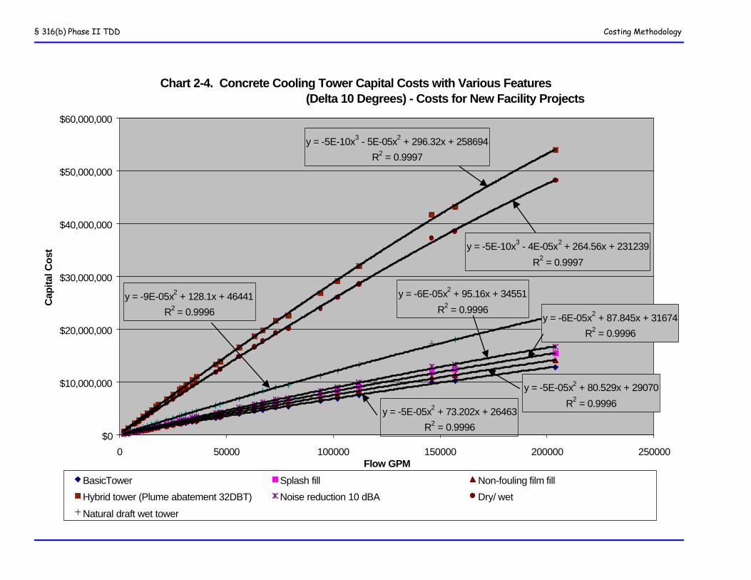
§ 316(b) Phase II TDD Costing Methodology
Chart 2-4. Concrete Cooling Tower Capital Costs with Various Features (Delta 10 Degrees) - Costs for New Facility Projects
y = -5E-10x3 - 4E-05x2 + 264.56x + 231239
R2 = 0.9997
y = -5E-10x3 - 5E-05x2 + 296.32x + 258694
R2 = 0.9997
y = -6E-05x2 + 95.16x + 34551
R2 = 0.9996y = -6E-05x2 + 87.845x + 31674
R2 = 0.9996
y = -5E-05x2 + 80.529x + 29070
R2 = 0.9996y = -5E-05x2 + 73.202x + 26463
R2 = 0.9996
y = -9E-05x2 + 128.1x + 46441
R2 = 0.9996
$0
$10,000,000
$20,000,000
$30,000,000
$40,000,000
$50,000,000
$60,000,000
0 50000 100000 150000 200000 250000Flow GPM
Cap
ital C
ost
BasicTower Splash fill Non-fouling film fill
Hybrid tower (Plume abatement 32DBT) Noise reduction 10 dBA Dry/ wet
Natural draft wet tower
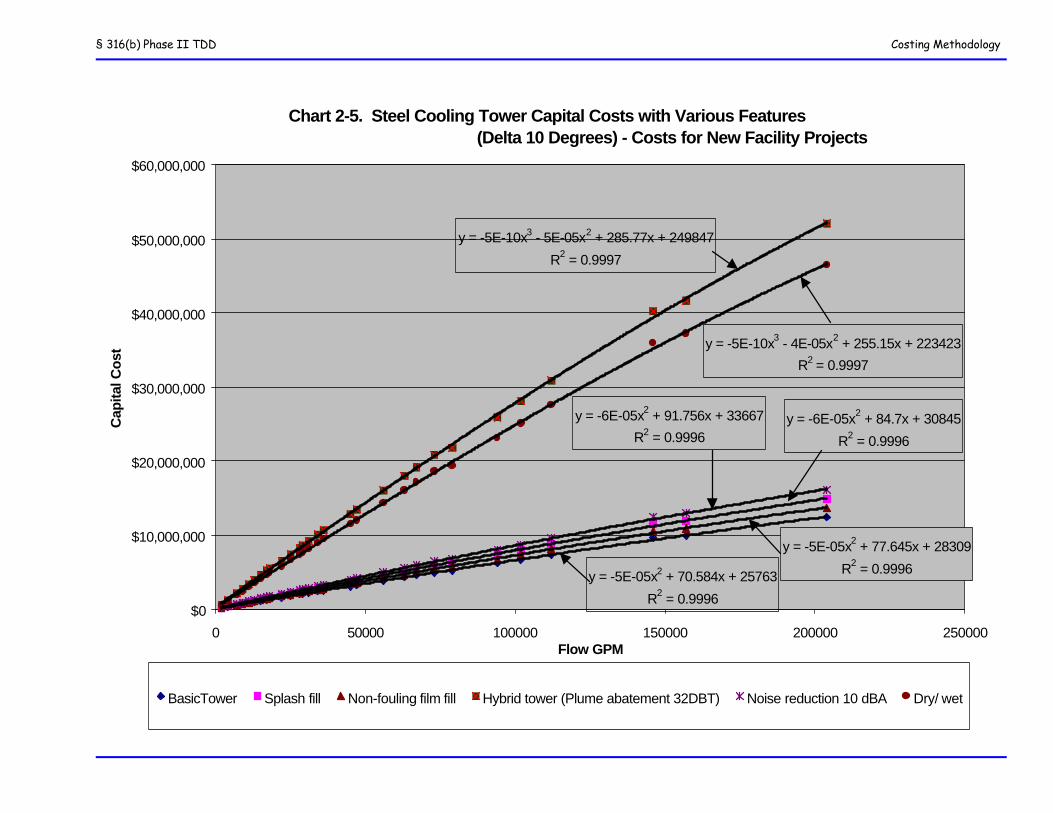
§ 316(b) Phase II TDD Costing Methodology
Chart 2-5. Steel Cooling Tower Capital Costs with Various Features (Delta 10 Degrees) - Costs for New Facility Projects
y = -5E-10x3 - 4E-05x2 + 255.15x + 223423
R2 = 0.9997
y = -5E-10x3 - 5E-05x2 + 285.77x + 249847
R2 = 0.9997
y = -6E-05x2 + 91.756x + 33667
R2 = 0.9996y = -6E-05x2 + 84.7x + 30845
R2 = 0.9996
y = -5E-05x2 + 77.645x + 28309
R2 = 0.9996y = -5E-05x2 + 70.584x + 25763
R2 = 0.9996$0
$10,000,000
$20,000,000
$30,000,000
$40,000,000
$50,000,000
$60,000,000
0 50000 100000 150000 200000 250000Flow GPM
Cap
ital C
ost
BasicTower Splash fill Non-fouling film fill Hybrid tower (Plume abatement 32DBT) Noise reduction 10 dBA Dry/ wet
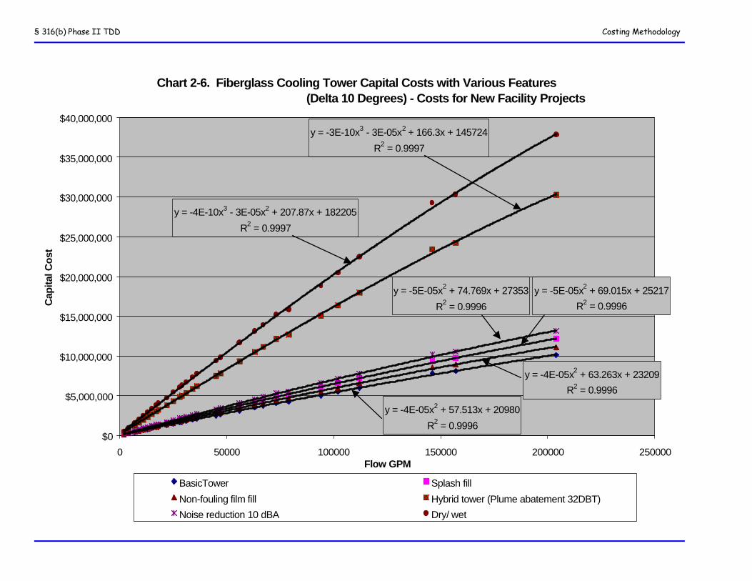
§ 316(b) Phase II TDD Costing Methodology
Chart 2-6. Fiberglass Cooling Tower Capital Costs with Various Features (Delta 10 Degrees) - Costs for New Facility Projects
y = -4E-10x3 - 3E-05x2 + 207.87x + 182205
R2 = 0.9997
y = -3E-10x3 - 3E-05x2 + 166.3x + 145724
R2 = 0.9997
y = -5E-05x2 + 74.769x + 27353
R2 = 0.9996
y = -5E-05x2 + 69.015x + 25217
R2 = 0.9996
y = -4E-05x2 + 63.263x + 23209
R2 = 0.9996
y = -4E-05x2 + 57.513x + 20980
R2 = 0.9996$0
$5,000,000
$10,000,000
$15,000,000
$20,000,000
$25,000,000
$30,000,000
$35,000,000
$40,000,000
0 50000 100000 150000 200000 250000Flow GPM
Cap
ital C
ost
BasicTower Splash fill
Non-fouling film fill Hybrid tower (Plume abatement 32DBT)
Noise reduction 10 dBA Dry/ wet
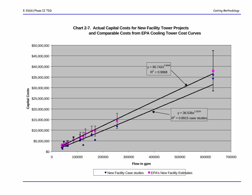
§ 316(b) Phase II TDD Costing Methodology
Chart 2-7. Actual Capital Costs for New Facility Tower Projects and Comparable Costs from EPA Cooling Tower Cost Curves
y = 36.536x1.0234
R2 = 0.8915 case studies
y = 90.742x0.9666
R2 = 0.9968
$0
$5,000,000
$10,000,000
$15,000,000
$20,000,000
$25,000,000
$30,000,000
$35,000,000
$40,000,000
$45,000,000
$50,000,000
0 100000 200000 300000 400000 500000 600000 700000
Flow in gpm
Cap
ital C
ost
s
New Facility Case studies EPA's New Facility Estimates
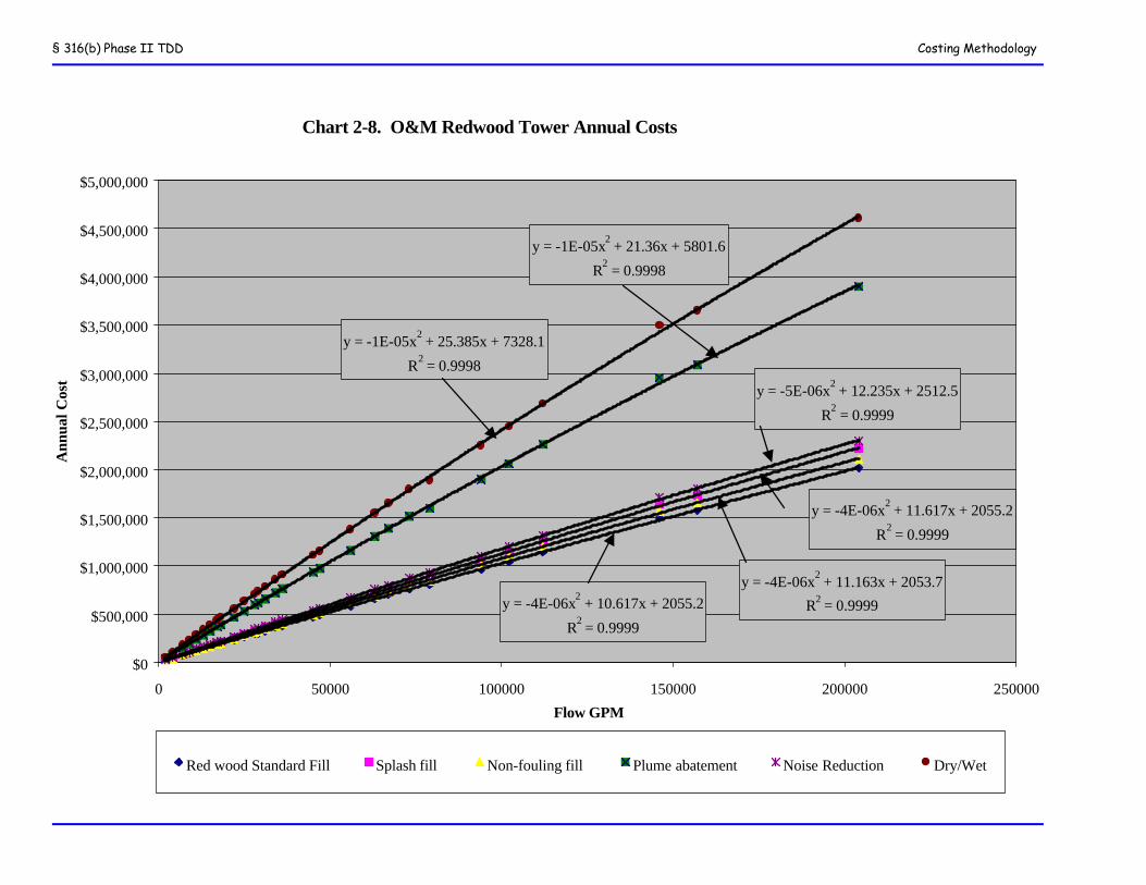
§ 316(b) Phase II TDD Costing Methodology
Chart 2-8. O&M Redwood Tower Annual Costs
y = -5E-06x2 + 12.235x + 2512.5
R2 = 0.9999
y = -1E-05x2 + 21.36x + 5801.6
R2 = 0.9998
y = -1E-05x2 + 25.385x + 7328.1
R2 = 0.9998
y = -4E-06x2 + 11.617x + 2055.2
R2 = 0.9999
y = -4E-06x2 + 10.617x + 2055.2
R2 = 0.9999
y = -4E-06x2 + 11.163x + 2053.7
R2 = 0.9999
$0
$500,000
$1,000,000
$1,500,000
$2,000,000
$2,500,000
$3,000,000
$3,500,000
$4,000,000
$4,500,000
$5,000,000
0 50000 100000 150000 200000 250000
Flow GPM
Ann
ual C
ost
Red wood Standard Fill Splash fill Non-fouling fill Plume abatement Noise Reduction Dry/Wet
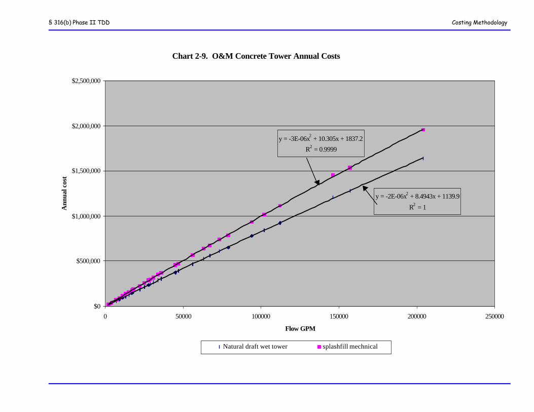
§ 316(b) Phase II TDD Costing Methodology
Chart 2-9. O&M Concrete Tower Annual Costs
y = -2E-06x2 + 8.4943x + 1139.9
R2 = 1
y = -3E-06x2 + 10.305x + 1837.2
R2 = 0.9999
$0
$500,000
$1,000,000
$1,500,000
$2,000,000
$2,500,000
0 50000 100000 150000 200000 250000
Flow GPM
Ann
ual c
ost
Natural draft wet tower splashfill mechnical
§ 316(b) Phase II TDD Appendix C
1 The Agency, however, obtained schematics of the Roseton Station retrofit design (1977) late in the development of this report. The design schematic by Central Hudson (1977, Exhibit 2) proposes nearly complete reuse of the existing circulating pipingsystem with minimal additional circulating piping required to connect the tower system. From the detailed schematic, EPAestimates that the lineal feet of new circulating water piping as less than 900 feet (that is, 2300 feet less than the Power Techdesign for Bowline Point Station). In addition, the Central Hudson schematic proposes for the existing intake discharge piping tobe completely reused, thereby eliminating the need for new makeup and blowdown piping. Therefore, significant piping andcivil works cost savings would be afforded for the Roseton Station over the comparably sized and situated Bowline Point Station. A rough estimate based on the detailed costs of Bowline Point developed by EPA would provide a total project capital costsavings of approximately $6 million.
C-1
Appendix C: Cost Estimate Report for a
Hypothetical Cooling System Conversion
The Agency conducted a detailed analysis of cost estimates for the hypothetical installation of a cooling towersystem at Bowline Point Station along the Hudson River in New York State. The Agency compared the results of itsanalysis to that included in the Draft Environmental Impact Statement (DEIS) of four Hudson River power plants.Power Tech Associates of New Jersey examined the costs of converting Bowline Point’s cooling system from once-through to recirculating in Appendix VIII-3 of the DEIS, which was submitted to New York State in December, 1999.Section IV-B of the DEIS contains detailed information on the existing cooling water system and site characteristics.The Power Tech report presents a narrative review of cooling tower technologies, a description of most key engineeringassumptions for and site characteristics affecting unit cost estimates, an environmental impact discussion of the coolingtowers, capital cost estimates at the aggregate level, and an economic analysis of these costs.
The focus of the Agency’s analysis was to develop detailed unit cost estimates for comparison to the PowerTech aggregate capital cost estimates. Although the Appendix VIII-3 cost estimates are at the aggregate level, the DEIS(in addition to historical engineering work on behalf of the four Hudson plants) provides sufficient detail to affordcomparison to detailed unit cost estimates developed by EPA. The sources of cost data and reference information forthe Agency’s unit cost estimates are presented below. The Agency chose to develop the detailed unit cost estimates forthe Bowline Plant, in order to examine the overall veracity of the estimates prepared by Power Tech Associates. TheAgency could have chosen to examine any of the four Hudson Plants, but selected Bowline because the degree of detailin the DEIS (and supporting documentation) was high and the uncertainty about site characteristics was the lowestamongst the four plants. For instance, the Agency had intended to also examine the Roseton Station, but was unableto determine the distance between the proposed towers and the condensers from the Power Tech report. In turn, theAgency was unable to develop detailed unit costs for the Roseton Station due to this key data omission.1
The Agency notes that the Mirant Bowline, LLC (the new owners and operators of Bowline Point Station)currrently are in the process of obtaining approval for expansion of the plant with planned construction of a third,combined-cycle unit on the site. If this construction commences as planned, the configuration of the plant would besignificantly altered. The land proposed by Power Tech Associates for construction of the cooling tower system forunits 2 and 3 (as analyzed herein) would likely be utilized in part for the new generating unit. Therefore, for this reasonand others, this analysis should be considered hypothetical in nature.
§ 316(b) Phase II TDD Appendix C
C-2
Bowline Point Station is a fossil-fueled plant cooled by a once-through system withdrawing from the HudsonRiver. The station is located approximately forty miles north of New York City in Haverstraw. The plant is locatedon a flat expanse of land. The property encompasses a cove (referred to as Bowline Pond) from which cooling wateris withdrawn. The station utilizes two steam generators, each sized at 622 megawatts, nameplate capacity. The unitswere installed in 1972 and 1974. Their utilization had slumped in the mid-1990s, with a rise shown after 1997. Theexisting once-through cooling system services two condensers at a maximum design flow rate of 1,110,000 gallons perminute (gpm). However, the plant generally operates with reduced pump usage for a design flow rate of 740,120 gpm.Both of these flow rates represent greater than one percent of the mean tidal flow as presented in the DEIS. The Agencynotes that in the facility’s response to the detailed questionnaire, Bowline Point reported a significantly lower flow ratefor its design intake flow than either capacity described here. In fact, the design intake flow reported by Bowline forthe detailed questionnaire was very similar to the average annual intake (in gallons per day) for the year 1998. In turn,the Agency intends to update its questionnaire response database to reflect the design flows above. This is an importantfact for the consideration of the Agency’s methodology for estimating costs of conversions from once-through torecirculating wet cooling systems (which is outlined in Chapter 2 of this document), as the Agency utilizes the designintake flow as the basis for assessing these costs.
The design circulating cooling flow estimated by Power Tech for the cooling towers is 642,000 gpm. PowerTech based their analysis on four-hybrid, wet-dry cooling towers each with 160,500 gpm of design circulating capacity.Power Tech states in Appendix VIII-3, page 10, “based on a conservative approach, the wet/dry mechanical draft towerwas chosen as the best way to evaluate economic…concerns associated with retrofitting cooling towers to the HudsonRiver plants.” As discussed in Grogan (2000), “a wet only (wet mechanical cooling tower) cooling water system willhave substantially less environmental impact and be less costly to the NY consumers. The trade-off is that the watervapor plume will be visible during more days of the year.” The Agency agrees with the Grogan assessment andconsiders the benefits of a wet/dry cooling system to be debatable for this installation. In 1977, Consolidated Edisonconducted a detailed study of the potential effects of a natural-draft wet (only) cooling tower on the local environmentnear the Roseton Generating Station. The analysis of plume effects from the natural-draft towers (each projected tobe about 400 ft tall) showed induced fogging at the station for a total of 85 hours per year, with a peak in February of40 hours (Con. Ed, 1977; Table 4-1). Outside of 0.8 miles from the station the study predicted 7 hours or less offogging, in any direction, for the entire year. Plume induced icing, according to the 1977 study, would occur for a totalof 45 hours in a single year at the station itself. Outside of 0.8 miles the total hours of icing for any nearby area wouldbe 6 hours or less per year. Because of the similarities in size and location between Roseton and Bowline Stations, theAgency considers these results to be relatively transferable to the Bowline Point location. However, the remote foggingand icing effects of a natural-draft tower system would be significantly greater than those for a comparably sizedmechanical-draft tower, which would be roughly 50 feet in height with a plume that is approximately 30 percent smallerthan that of a natural-draft tower. In addition, Central Hudson, et al. (1977) quantified the economic impacts of theseeffects in the Report on Cost-Benefit Analysis of Operation of Hudson River Steam-Electric Units with Once-throughand Closed-cycle Cooling Systems. In the report the authors state, “the impact of the operation of the proposed closed-cycle cooling systems in terms of induced fog and icing is not expected to be substantial.” This summary refers to thecombined total of the four power plants potentially converting to natural-draft wet cooling tower systems. The effectsfor less than four plants (or a single plant) converting to a mechanical-draft wet cooling tower system would be evenless pronounced. Therefore, based on these 1977 analyses by Con. Ed. and Central Hudson, et al., the Agencyconsiders the mechanical draft wet (only) cooling towers to be a viable option for Bowline Point.
§ 316(b) Phase II TDD Appendix C
C-3
Regardless of the configuration of the tower (that is, wet only or hybrid, wet-dry), the cooling flow would beequivalent between the two types. Additionally, the land requirements, site preparation, and civil construction wouldbe nearly identical for both types of tower installations, with the exception of potential support piling requirements.For the wet-dry models, marginal additional support piling (due to increased load) may be necessary. The Agency, inits analysis, has estimated all costs based on mechanical-draft wet (only) cooling towers.
Bowline Point is located roughly 30 miles from Poughkeepsie, NY, which is one of the nearest towns toBowline included in the city cost index of R.S. Means. The R.S. Means City Cost Index contains other towns in thevicinity of Haverstraw in addition to Poughkeepsie, such as Suffern and White Plains. Haverstraw is, in effect,equidistant from each of these three cities. Poughkeepsie’s cost index represents the median and near to the averageof these three surrounding city cost indexes. Therefore, the Agency utilized costs index multipliers specific to themedian of these three cities for its cost estimates. The DEIS states that truck traffic through Haverstraw would bedisruptive to the town, which the Agency cannot dispute. Therefore, in all cases, the Agency estimated the haulingrequirements as conservative (that is, small to medium trucks) and to account for alternative routing (that is, long round-trips) to minimize and avoid town traffic disruptions. Additionally, the Bowline Point site covers 245 acres. Basedon the detailed aerial photographs (proprietary photos published by www.mapquest.com and available to the generalpublic through the website, but not for publication), significant available land for staging of constructionoperations is available.
Power Tech estimates that the cooling tower system would occupy a total of 6 acres. However, theyassert that 13 acres would require clearing and preparation for construction. The plot of land projected forconstruction would be approximately 800 feet east of the generators in a relatively low-lying, flat area. PowerTech assert that this plot of land is populated by second-growth timber. Detailed aerial photographs revealbrush and small trees covering approximately half of the 13 acres. Additionally, the Power Tech report assertsthat the land shows signs of being wetlands, but the body of the DEIS states that the NY DEC does not designateany wetland areas on the Bowline Point property. The USDA soil survey included in Appendix IV-B.1-1indicates that the tower would be constructed in part urban land, part wet substratum. Based on these factors,the Agency’s analysis estimates that significant dewatering control and foundation piling would be required forthe construction project.
The existing intake structure is a surface shoreline intake located to the south and west of the generatorunits. The intake pumps sit immediately behind the intake screens, and, due to a lack of proximity, would notbe of use for circulating cooling water between the projected cooling tower location and the condensers. Theintake and discharge piping passes approximately 150 meters immediately to the east of the generator house andbends southwesterly to and from the discharge and intake. This piping is in relatively close proximity to theprojected location of the cooling towers and could be used for a retrofit design, though, notably, Power Tech doesnot address this prospect in their engineering assessment. In turn, the detailed cost estimates included in this fileestimate that only the existing intake and discharge structures will be used for the conversion design and minimalexisting piping will be utilized. Based on the example cooling system conversion cases discussed in Chapter 4,the Agency views this design as potentially unrealistic and perhaps overly conservative with respect to capitalcosts. In addition, as discussed in footnote 1 above, the detailed engineering schematics the Agency obtained for
§ 316(b) Phase II TDD Appendix C
2 In the Agency’s view, Appendix VIII-3 incorrectly states the tax rate for New York State, double-counts contractor profit, anddouble-counts freight and insurance on materials.
C-4
the historical, proposed Roseton Generating Station cooling system conversion show significant reuse of existingcirculating water piping for that design.
Based on the detailed description provided in the DEIS, the existing intake bays present flexibility forconverting to a reduced intake flow for makeup cooling water. Because the intake is comprised of 6 separate bayswith dedicated pumping stations, several of the bays could be retrofitted with a reduced size pump or a newvariable speed motor to provide makeup water to the cooling towers. The piping delivery to the tower could beconfigured to branch from the existing piping. Other configurations that maintain the capability to return toonce-through cooling could be examined (such as diverting the flow from two bays to the makeup piping andretaining the other four bays for peak-demand, once-through operation). For the Agency’s conservative analysis,the design assumes demolition and replacement of three intake pumps, in addition to construction of wholly newintake and discharge piping.
The subject of plant outage for conversion of the cooling system is addressed in Appendix VIII-3 of theDEIS (page 19), where Power Tech states, “it was assumed that each of the [Bowline and Roseton] plants wouldexperience about one month of outage during the winter months.” EPA notes that several data sources indicatethat the outages could be appreciably lower than this estimate. One data source is an engineering report onRoseton Station from Central Hudson Gas & Electric Corporation (July 1977), which estimates, “as aconservative approach…the downtime cost was calculated for one (1) unit and for ten (10) days,” to convert froma once-through to recirculating cooling system. Additionally, the Agency obtained two empirical examples ofcooling system conversion projects with durations in one-case significantly less than thirty days and 83 hours inthe other (as discussed in the Chapter 4).
The results of the Agency’s detailed cost analysis for Bowline Point show that the capital cost estimatespresented in Appendix VIII-3 of the DEIS overstate the potential cost to convert from a once-through torecirculating cooling system. The Agency did not compare each line item of the Power Tech prepared capitalcosts in Appendix VIII, but, rather, focused on the civil works estimates. The Agency prepared two sets of costestimates: high unit costs and moderate unit costs. The Agency based the high unit costs on extremelyconservative assumptions for design variables. The moderate costs are also conservative, but utilize optimizeddesign variables that would reflect a moderate engineering cost estimate. In both cases, the Agency’s analysisdemonstrates that the Power Tech estimates overstate direct capital costs by approximately 24 to 36 percent.Further, the Agency disagrees with several estimates of project overhead rates used by Power Tech.2
Considering the total project costs differences, in the Agency’s view, the Appendix VIII-3 estimates mayoverstate total project capital costs by 31 to 42 percent. As described above, the Agency disputes the utility ofthe wet-dry, hybrid tower for this location. The Agency considers the incorporation of this technology into theDEIS analysis, as stated in Appendix VIII, to be an overly conservative approach. The Agency’s analysis,therefore, focuses on the wet only mechanical draft tower system. However, had the Agency incorporated thePower Tech cost estimates for the wet-dry, hybrid system, the Appendix VIII-3 total project capital costs wouldremain overestimated by 20 to 30 percent, according to the Agency’s analysis. Table C-1 shows the Agency’sunit cost estimates as compared to those included in Appendix VIII-3 of the DEIS.
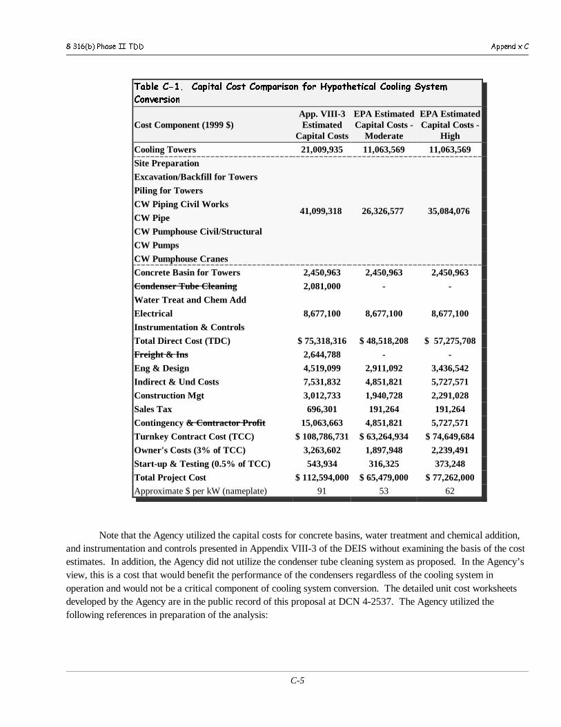
§ 316(b) Phase II TDD Appendix C
C-5
Table C-1. Capital Cost Comparison for Hypothetical Cooling System
Conversion
Cost Component (1999 $)App. VIII-3Estimated
Capital Costs
EPA EstimatedCapital Costs -
Moderate
EPA EstimatedCapital Costs -
High
Cooling Towers 21,009,935 11,063,569 11,063,569
Site Preparation
41,099,318 26,326,577 35,084,076
Excavation/Backfill for Towers
Piling for Towers
CW Piping Civil Works
CW Pipe
CW Pumphouse Civil/Structural
CW Pumps
CW Pumphouse Cranes
Concrete Basin for Towers 2,450,963 2,450,963 2,450,963
Condenser Tube Cleaning 2,081,000 - -
Water Treat and Chem Add
8,677,100 8,677,100 8,677,100Electrical
Instrumentation & Controls
Total Direct Cost (TDC) $ 75,318,316 $ 48,518,208 $ 57,275,708
Freight & Ins 2,644,788 - -
Eng & Design 4,519,099 2,911,092 3,436,542
Indirect & Und Costs 7,531,832 4,851,821 5,727,571
Construction Mgt 3,012,733 1,940,728 2,291,028
Sales Tax 696,301 191,264 191,264
Contingency & Contractor Profit 15,063,663 4,851,821 5,727,571
Turnkey Contract Cost (TCC) $ 108,786,731 $ 63,264,934 $ 74,649,684
Owner's Costs (3% of TCC) 3,263,602 1,897,948 2,239,491
Start-up & Testing (0.5% of TCC) 543,934 316,325 373,248
Total Project Cost $ 112,594,000 $ 65,479,000 $ 77,262,000
Approximate $ per kW (nameplate) 91 53 62
Note that the Agency utilized the capital costs for concrete basins, water treatment and chemical addition,and instrumentation and controls presented in Appendix VIII-3 of the DEIS without examining the basis of the costestimates. In addition, the Agency did not utilize the condenser tube cleaning system as proposed. In the Agency’sview, this is a cost that would benefit the performance of the condensers regardless of the cooling system inoperation and would not be a critical component of cooling system conversion. The detailed unit cost worksheetsdeveloped by the Agency are in the public record of this proposal at DCN 4-2537. The Agency utilized thefollowing references in preparation of the analysis:
§ 316(b) Phase II TDD Appendix C
C-6
References Used in the Cost Analysis:
J.M. Burns and Michilletti, W.C., 2000, "Comparison of Wet and Dry Cooling Systems for Combined Cycle PowerPlants," Appendix F to the Comments of the Utility Water Act Group (UWAG) on EPA's Proposed Sec. 316(b)Rule for New Facilities.
J.M. Burns and Tsou, J.L., 2001, "Modular Steam Condenser Replacement Using Corrosion Resistant HighPerformance Stainless Steel Tubing," Proceedings of the 2001 Conference of the American Society of MechanicalEngineers.
Central Hudson Gas & Electric Corporation, 1977, "Engineering, Environmental (Non-Biological), and EconomicAspects of a Closed-Cycle Cooling System," Roseton Generating Station.
Central Hudson Gas & Electric Corporation, et al., July 1977, "Report on Cost-Benefit Analysis of Operation ofHudson River Steam-Electric Units with Once-through and Closed-cycle Cooling Systems," prepared by Mathtech,Inc., a subsidiary of Mathematica, Inc.
Central Hudson Gas & Electric Corp., et al., 1994, "Utility Responses to New York State Department ofEnvironmental Conservation/Tellus Institute Commnets and Questions on Preliminary DEIS for SPDES Permitsfor Indian Point 2 and 3, Bowline, and Roseton Power Plants."
Central Hudson Gas & Electric Corp., et al., December 1999, "Draft Environmental Impact Statement for StatePollutant Discharge Elimination System Permits for Bowline Point, Indian Point 2 & 3, and Roseton Steam ElectricGenerating Stations."
Consolidated Edison Company of New York, Inc., 1977, "Environmental Analysis of Natural Draft CoolingTowers for Roseton Generating Station," prepared for Central Hudson Gas & Electric Corp.
Construction Industry Institute, 2001, "Benchmarking & Metrics Analysis Results - What is the AverageContingency for Heavy Industrial Projects?" http://www.cii-benchmarking.org/news/contingency.htm, Austin,Texas.
Engineering News-Record, 2002, "Construction Cost Index History (1908-2002),"http://www.enr.com/cost/costcci.asp, McGraw-Hill, Inc., New York.
D.B. Grogan Associates, Inc., 2000, "Hudson River Power Plants - Cooling Water Design Assessment,"prepared on behalf of ESSA Technologies, Ltd. for support of the New York State Department ofEnvironmental Conservation.
S.H. Kosmatka and Panarese, W.C., 1992, "Design and Control of Conrete Mixtures, Thirteenth Edition"Portland Cement Association, Skokie, Illinois.
W.L. McCabe, et al., 1985, "Unit Operations of Chemical Engineering, Fourth Edition," McGraw-Hill, Inc.,New York.

§ 316(b) Phase II TDD Appendix C
C-7
Page, J. R., Senior Editor, 1998, "RS Means Heavy Construction Cost Data, 12th Edition," R.S. MeansCompany, Inc.
Parsons Infrastructure and Technology, 1998, "Market-Based Advanced Coal Power Systems," Parsonsreport no. 10198, Reading, Pennsylvania.
M.S. Peters and Timmerhaus, K.D., 1991, "Plant Design and Economics for Chemical Engineers, FourthEdition," McGraw-Hill, Inc., New York.
U.S. Army Corps of Engineers, 1998, "Conduits, Culverts, and Pipes," engineer manual 1110-2-2902.
USGen New England, 2001, "Section 316b Demonstration Report," submitted to the New England InterstateWater Pollution Control Commission.
Waier, P. R., Senior Editor, 2000, "RS Means Building Construction Cost Data, 58th Edition," R.S. MeansCompany, Inc.

§ 316(b) Phase II TDD Appendix C
C-8
THIS PAGE INTENTIONALLY LEFT BLANK
§ 316(b) Phase II TDD Dry Cooling
D - 1
Appendix D: Dry Cooling
INTRODUCTION
This appendix presents a synopsis of the design and operation of an air-cooled condenser system (dry cooling) and itsapplicability for existing power plants. The majority of the background information included in this discussion on drycooling is from references listed at the end of this appendix, the background discussion draws primarily from Burnsand Michiletti, 2000.
Dry cooling systems transfer heat to the atmosphere without the evaporative loss of water. There are two types of drycooling systems for power plant applications: direct-dry cooling and indirect-dry cooling. Direct-dry cooling systemsutilize air to directly condense steam, while indirect dry cooling systems utilize a closed-cycle water cooling system tocondense steam, and the heated water is then air cooled. In the Agency’s determination, indirect-dry cooling generallyis the only application of the technology that would be considered for retrofit situations at existing power plants becausea condenser would already be in place for a once-through or recirculated cooling system. For dry cooling towers theturbine exhaust steam exits directly to an air-cooled, finned-tube condenser. In the Agency’s view, if this applicationwould be applied to an existing plant, the entire steam turbine would necessarily be replaced or reconfigured in anunprecedented fashion. The costs of steam turbines are significantly more expensive than any type of recirculatingcooling system, including the dry cooling systems. The Agency has determined that the feasibility of direct-dry coolingsystems for existing plants is not demonstrated and because of the limitations and potential costs is not a candidate forretrofit situations. Therefore, the Agency does not further consider direct-dry cooling systems for existing facilities,though they are referred to significantly throughout the remainder of this appendix. Because direct-dry cooling systemswould be more efficient and less costly than indirect-systems (ignoring the feasibility issues addressed above), theAgency’s analyses of dry cooling systems using direct-dry cooling systems would show increased energy penalties andsignficantly higher costs.
For indirect-dry cooled systems, recirculating fluid (usually water) passes through an air-cooled, finned tube tower. Incontrast to direct-dry cooling, indirect-dry cooling does not operate as an air-cooled condenser. In other words, thesteam is not condensed within the structure of the dry cooling tower, but instead indirectly through an indirect heatexchanger (that is, a surface condenser). Therefore, the indirect-dry cooling system would need to overcome additionalheat resistance in the shell of the condenser compared to the direct dry cooling system. Ultimately, the inefficiencypenalties of indirect dry cooling systems will exceed those of direct-dry cooling systems in all cases. Similar to thedirect-dry cooling systems, the arrangement of the finned tubes are most generally of an A-frame pattern (which reducesthe land area required compared to other configurations). However, due to the fact that dry cooling towers do notevaporate water for heat transfer, the towers are quite large in comparison to similarly sized wet cooling towers.Additionally, because indirect-dry cooled systems also utilize a surface condenser, with additional heat transferinefficiencies compared to a direct-dry cooled system, the indirect systems are generally considered to be significantlylarger than direct systems for comparable heat loads. Because dry cooling towers rely on sensible heat transfer, a largequantity of air must be forced across the finned tubes by fans to improve heat rejection. The number of fans is thereforeconsiderably larger than would be used in a mechanical-draft wet cooling tower.
The key feature of dry cooling systems is that no evaporative cooling or release of heat to surface water occurs. Asa result, water consumption rates are very low compared to wet cooling systems. Since the unit does not rely in
§ 316(b) Phase II TDD Dry Cooling
D - 2
principle on evaporative cooling as does a wet cooling tower, larger volumes of air must be passed through the systemcompared to the volume of air used in wet cooling towers. As a result, dry cooling towers need larger heat transfersurfaces and, therefore, tend to be larger in size than comparable wet cooling towers. The design and performance ofthe dry cooling system is based on the ambient dry bulb temperature. The dry bulb temperature is higher than the wetbulb temperature under most circumstances, being equal to the wet bulb temperature only when the relative humidityis at 100%.
Direct-dry cooling has been installed at a variety of power plants utilizing many fuel types. In the United States, drycooling is most frequently applied at plants in northern climates. Additionally, arid areas with significant water scarcityconcerns have also experiencing growth in dry cooling system projects. However, each of the demonstrations that theAgency has studied is for a direct-dry cooling system configured for a new facility project. As demonstrated in Chapter5, the comparative energy penalty of a direct-dry cooling plant in a hot environment at peak summer conditions canexceed 12 percent. Additionally, the indirect-dry cooling system would be even less efficient, producing maximumenergy penalties of 18 percent according to the Department of Energy (DOE, 2001). Additionally, indirect-dry coolingsystems would likely cause prohibitively high exhaust turbine backpressures, thereby potentially debilitating theoperation of some plants at peak-summer, peak-demand conditions (DOE, 2001).
As with wet cooling towers, the ambient air temperature and system design can have an effect on the steam turbineexhaust pressure, which in turn affects the turbine efficiency. Thus, the turbine efficiency can change over time as theair temperature changes. The fans used to mechanically force air through the condenser represent the greatestoperational energy requirement for dry cooling systems.
A design measure comparable to the approach value used in wet towers is the difference between the design dry bulbtemperature and the temperature of saturated steam at the design turbine exhaust pressure. In general, for direct-drycooling systems a larger, more costly dry cooling system will produce a smaller temperature difference across the drycooling tower and, therefore, a lower turbine exhaust pressure. However, as calculated by DOE, the 40 degree Fapproach indirect-dry cooling towers may actually be less efficient than smaller sized 20 degree F towers in the casesmodeled by DOE.
Steam turbines are designed to operate within certain exhaust pressure ranges. In general, steam turbines that aredesigned to operate at the exhaust steam pressure ranges typical of wet cooling systems, which generally operate atlower exhaust pressures (e.g., <5 in Hg), may be damaged if the exhaust pressure exceeds a certain value. Even thehighest values of operable exhaust pressures may be exceed with retrofitted indirect-dry cooling systems. For existingfacilities, many with aged turbines, this is a fundamental engineering problem for the feasibility of the retrofitted drycooling system.
In an analysis for the New Facility rule, EPA examined turbine exhaust pressures at the highest design dry bulbtemperatures in the U.S. (which were around 100 °F), which ranged from 5.0 to 9.5 inches Hg. The highest value of9.5 inches Hg was for a refinery power system in California which, based on the steam rate, was comparable to otherrelatively small systems generating several megawatts and apparently did not warrant the use of an efficient coolingsystem. The other data showed turbine exhaust pressures of around 6 to 7 inches Hg at dry bulb temperatures ofaround 100 °F. Maximum exhaust pressures in the range of 8 to12 inches Hg may be expected in hotter regions of theU.S.(Hensley 1985). An air cooled condenser analysis (Weeks 2000) reports that for a combined cycle plant built inBoulder City, Nevada, the maximum ambient temperature used for the maximum off-design specification was 108 °Fwith a corresponding turbine exhaust pressure of 7.8 inches Hg. Note that the equation used by EPA to generate theturbine exhaust pressure values in the energy penalty analysis produced an estimated exhaust pressure of 8.02 inchesHg at a dry bulb temperature of 108 °F. For wet towers, the typical turbine exhaust pressure operating range is1.5 to
§ 316(b) Phase II TDD Dry Cooling
D - 3
3.5 inches Hg(Woodruff 1998). EPA prepared all of this analysis in the context of direct-dry cooling systems installedat new facility projects. For hypothetical indirect-dry systems at existing facilities, the backpressures would besignificantly higher than the values examined by the Agency for the New Facility rule.
In addition, the issue of demonstrated dry cooling systems (even for new facilities) emerges in the context of fossil-fueland nuclear plants. The largest operating coal-fired plant in the United States with dry cooling is the Wyodak Stationin Gillette, WY with a total cooling capacity of 330 MW (1.88 million lb/hr of steam). EPA notes that this issignificantly smaller than a vast number of coal-fired plants within the scope of this proposal. In addition, the designtemperature of the direct-dry cooled system at this plant (which directly affects the size of the dry cooling system) isbelow average for summer conditions throughout the United States (the Wyodak Station has a design temperature of66 deg F). The Agency reiterates its reservation of applying requirements based on dry cooling at the sizes of coal-firedand nuclear plants in the scope of this proposal.
Costs of Dry Cooling
For the New Facility Final Rule, the Agency projected that the total annualized cost for the dry cooling alternative was$490 million (in 2000 dollars) for 121 facilities. This proposed rule applies to 539 facilities, and therefore, a regulatoryoption based on dry cooling for all plants would impose a dramatically higher annual compliance cost than thatestimated for the New Facility Final Rule. In addition, the costs the dry cooling system would be even more dramatic,due to the fact that the majority of existing facilities within the scope of this rule operate with once-through coolingsystems, whereas for the New Facility Final Rule, the vast majority of plants were projected to install recirculating wetcooling at baseline, thereby reducing marginal cost increases.
Although the dry cooling option is extremely effective at reducing impingement and entrainment and would yield annualbenefits of $138.2 million for impingement reductions and $1.33 billion for entrainment reductions at existing facilities,it does so at a cost that would be unacceptable. EPA recognizes that dry cooling technology uses extremely low-levelor no cooling water intake, thereby reducing impingement and entrainment of organisms to dramatically low levels.However, EPA interprets the use of the word “minimize” in section 316(b) in a manner that allows EPA the discretionto consider technologies that very effectively reduce, but do not completely eliminate, impingement and entrainment andtherefore meet the requirements of section 316(b). Although EPA has rejected dry cooling technology as a nationalminimum requirement, EPA does not intend to restrict the use of dry cooling or to dispute that dry cooling may be theappropriate cooling technology for some facilities. For example, facilities that are repowering and replacing the entireinfrastructure of the facility may find that dry cooling is an acceptable technology in some cases. A State may chooseto use its own authorities to require dry cooling in areas where the State finds its fishery resources need additionalprotection above the levels provided by these technology-based minimum standards.
Methodology for Dry Cooling Cost Estimates at Existing Facilities
For the purposes of approximating the hypothetical costs of retrofitting to dry cooling for existing facilities, the Agencyused the following methodology for developing facility-level costs estimates:
• Capital costs for the dry cooling towers were estimated using the cost equation that was developed for the NewFacility Rule (see the next section for the New Facility dry cooling cost estimates).
• The cost equations are based on equivalent cooling water flow rates (gpm) using the once-through design intakecooling flow as the independent variable. To aviod using the equation outside of its valid range, for facilities with
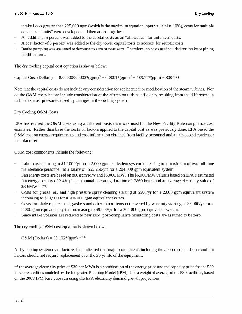
§ 316(b) Phase II TDD Dry Cooling
D - 4
intake flows greater than 225,000 gpm (which is the maximum equation input value plus 10%), costs for multipleequal size “units” were developed and then added together.
• An additional 5 percent was added to the capital costs as an “allowance” for unforseen costs. • A cost factor of 5 percent was added to the dry tower capital costs to account for retrofit costs.• Intake pumping was assumed to decrease to zero or near zero. Therefore, no costs are included for intake or piping
modifications.
The dry cooling capital cost equation is shown below:
Capital Cost (Dollars) = -0.00000000008*(gpm) 3 + 0.0001*(gpm) 2 + 189.77*(gpm) + 800490
Note that the capital costs do not include any consideration for replacement or modification of the steam turbines. Nordo the O&M costs below include consideration of the effects on turbine efficiency resulting from the differences inturbine exhaust pressure caused by changes in the cooling system.
Dry Cooling O&M Costs
EPA has revised the O&M costs using a different basis than was used for the New Facility Rule compliance costestimates. Rather than base the costs on factors applied to the capital cost as was previously done, EPA based theO&M cost on energy requirements and cost information obtained from facility personnel and an air-cooled condensermanufacturer.
O&M cost components include the following:
• Labor costs starting at $12,000/yr for a 2,000 gpm equivalent system increasing to a maximum of two full timemaintenance personnel (at a salary of $55,250/yr) for a 204,000 gpm equivalent system.
• Fan energy costs are based on 800 gpm/MW and $6,000/MW. The $6,000/MW value is based on EPA’s estimatedfan energy penalty of 2.4% plus an annual operating duration of 7860 hours and an average electricity value of$30/MW-hr**.
• Costs for grease, oil, and high pressure spray cleaning starting at $500/yr for a 2,000 gpm equivalent systemincreasing to $19,500 for a 204,000 gpm equivalent system.
• Costs for blade replacement, gaskets and other minor items not covered by warranty starting at $3,000/yr for a2,000 gpm equivalent system increasing to $9,600/yr for a 204,000 gpm equivalent system.
• Since intake volumes are reduced to near zero, post-compliance monitoring costs are assumed to be zero.
The dry cooling O&M cost equation is shown below:
O&M (Dollars) = 53.122*(gpm) 0.8442
A dry cooling system manufacturer has indicated that major components including the air cooled condenser and fanmotors should not require replacement over the 30 yr life of the equipment.
** the average electricity price of $30 per MWh is a combination of the energy price and the capacity price for the 530in-scope facilities modeled by the Integrated Planning Model (IPM). It is a weighted average of the 530 facilities, basedon the 2008 IPM base case run using the EPA electricity demand growth projections.
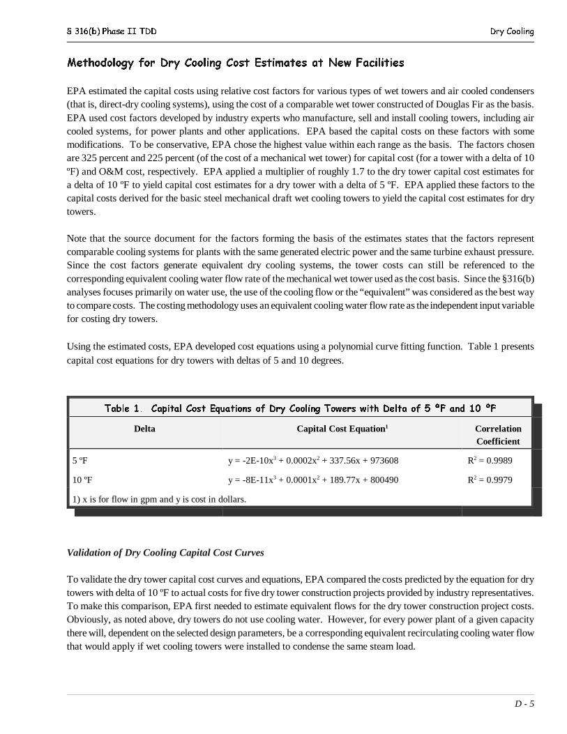
§ 316(b) Phase II TDD Dry Cooling
D - 5
Methodology for Dry Cooling Cost Estimates at New Facilities
EPA estimated the capital costs using relative cost factors for various types of wet towers and air cooled condensers(that is, direct-dry cooling systems), using the cost of a comparable wet tower constructed of Douglas Fir as the basis.EPA used cost factors developed by industry experts who manufacture, sell and install cooling towers, including aircooled systems, for power plants and other applications. EPA based the capital costs on these factors with somemodifications. To be conservative, EPA chose the highest value within each range as the basis. The factors chosenare 325 percent and 225 percent (of the cost of a mechanical wet tower) for capital cost (for a tower with a delta of 10ºF) and O&M cost, respectively. EPA applied a multiplier of roughly 1.7 to the dry tower capital cost estimates fora delta of 10 ºF to yield capital cost estimates for a dry tower with a delta of 5 ºF. EPA applied these factors to thecapital costs derived for the basic steel mechanical draft wet cooling towers to yield the capital cost estimates for drytowers.
Note that the source document for the factors forming the basis of the estimates states that the factors representcomparable cooling systems for plants with the same generated electric power and the same turbine exhaust pressure.Since the cost factors generate equivalent dry cooling systems, the tower costs can still be referenced to thecorresponding equivalent cooling water flow rate of the mechanical wet tower used as the cost basis. Since the §316(b)analyses focuses primarily on water use, the use of the cooling flow or the “equivalent” was considered as the best wayto compare costs. The costing methodology uses an equivalent cooling water flow rate as the independent input variablefor costing dry towers.
Using the estimated costs, EPA developed cost equations using a polynomial curve fitting function. Table 1 presentscapital cost equations for dry towers with deltas of 5 and 10 degrees.
Table 1. Capital Cost Equations of Dry Cooling Towers with Delta of 5 ºF and 10 ºF
Delta Capital Cost Equation1 CorrelationCoefficient
5 ºF y = -2E-10x3 + 0.0002x2 + 337.56x + 973608 R2 = 0.9989
10 ºF y = -8E-11x3 + 0.0001x2 + 189.77x + 800490 R2 = 0.9979
1) x is for flow in gpm and y is cost in dollars.
Validation of Dry Cooling Capital Cost Curves
To validate the dry tower capital cost curves and equations, EPA compared the costs predicted by the equation for drytowers with delta of 10 ºF to actual costs for five dry tower construction projects provided by industry representatives.To make this comparison, EPA first needed to estimate equivalent flows for the dry tower construction project costs.Obviously, as noted above, dry towers do not use cooling water. However, for every power plant of a given capacitythere will, dependent on the selected design parameters, be a corresponding equivalent recirculating cooling water flowthat would apply if wet cooling towers were installed to condense the same steam load.

§ 316(b) Phase II TDD Dry Cooling
D - 6
EPA used the steam load rate and cooling system efficiency to determine the equivalent flow. Note that the heatrejection rate will be proportional to the plant capacity. EPA estimated the flow required for a wet cooling tower thatis functionally equivalent to the dry tower by converting each plant’s steam tons/hour into cooling flow in gpm usingthe following equations:
Steam tons/hr x 2000 lbs/ton x 1000 BTUs/lb steam = BTUs/hrOne ton/hr = 12,000 BTU/hrBTUs/hr / 12000 = Tons of ice Tons of Ice x 3 = Flow (gpm) for wet systems
Chart 4-2 presents a comparison of the EPA capital cost estimates for dry towers with delta of 10 ºF (with 25% errorbars) to actual dry tower installations. This chart shows that EPA’s cost curves produce conservative cost estimates,since the EPA estimates are greater than all of the dry tower project costs based on the calculated equivalent coolingflow rate for the actual projects.
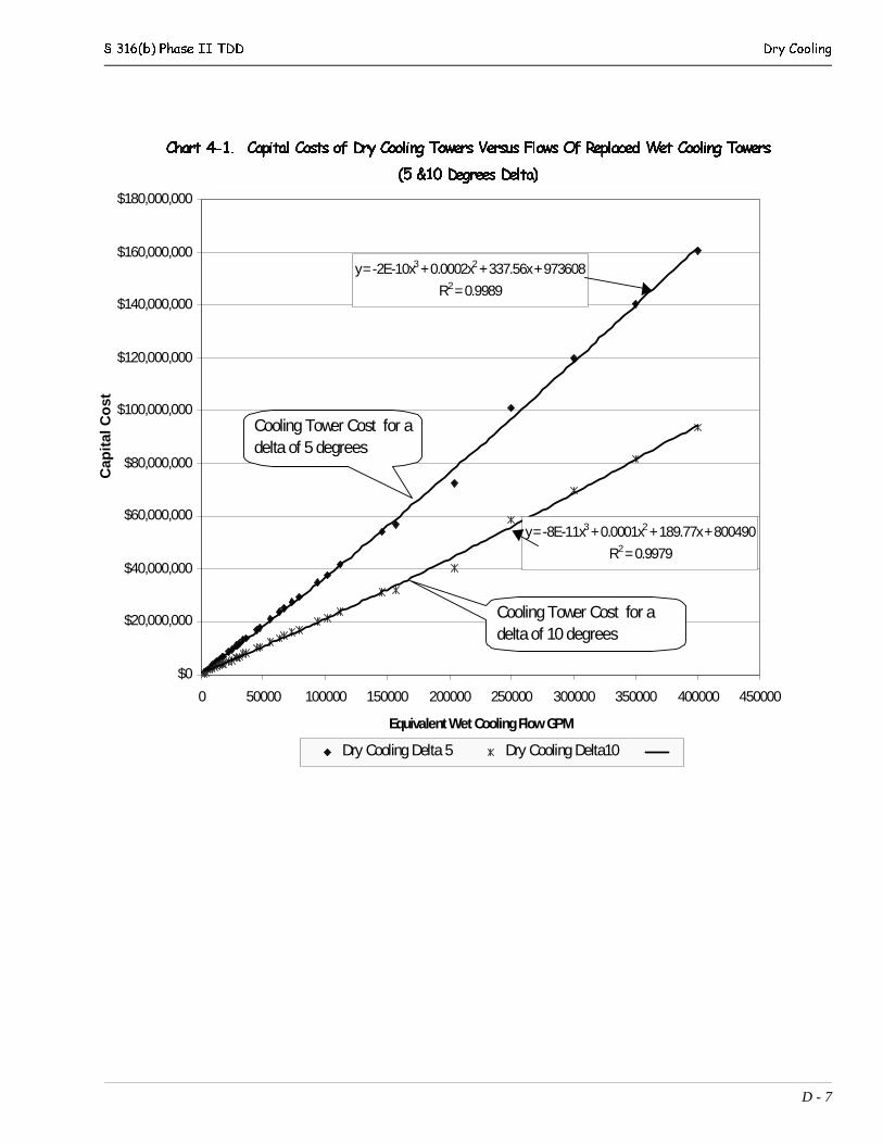
§ 316(b) Phase II TDD Dry Cooling
D - 7
Chart 4-1. Capital Costs of Dry Cooling Towers Versus Flows Of Replaced Wet Cooling Towers
(5 &10 Degrees Delta)
y = -2E-10x3 + 0.0002x2 + 337.56x + 973608
R2 = 0.9989
y = -8E-11x3 + 0.0001x2 + 189.77x + 800490
R2 = 0.9979
$0
$20,000,000
$40,000,000
$60,000,000
$80,000,000
$100,000,000
$120,000,000
$140,000,000
$160,000,000
$180,000,000
0 50000 100000 150000 200000 250000 300000 350000 400000 450000
Equivalent Wet Cooling Flow GPM
Cap
ital
Co
st
Dry Cooling Delta 5 Dry Cooling Delta10
Cooling Tower Cost for a delta of 5 degrees
Cooling Tower Cost for a delta of 10 degrees
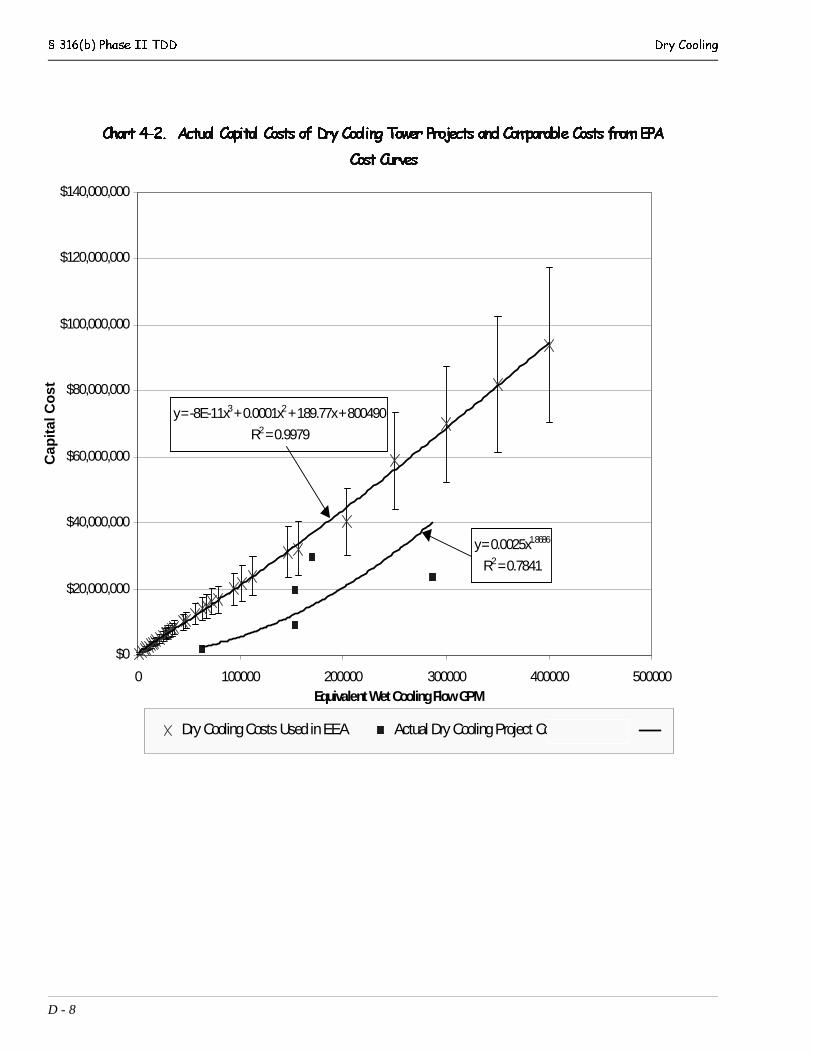
§ 316(b) Phase II TDD Dry Cooling
D - 8
Chart 4-2. Actual Capital Costs of Dry Cooling Tower Projects and Comparable Costs from EPA
Cost Curves
y = -8E-11x3 + 0.0001x2 + 189.77x + 800490
R2 = 0.9979
y = 0.0025x1.8686
R2 = 0.7841
$0
$20,000,000
$40,000,000
$60,000,000
$80,000,000
$100,000,000
$120,000,000
$140,000,000
0 100000 200000 300000 400000 500000Equivalent Wet Cooling Flow GPM
Cap
ital
Co
st
Dry Cooling Costs Used in EEA Actual Dry Cooling Project Costs
§ 316(b) Phase II TDD Dry Cooling
D - 9
EVALUATION OF DRY COOLING AS BTA
This section presents a summary of EPA’s evaluation of the dry cooling technology as a candidate for best technologyavailable to minimize adverse environmental impacts. Based on the information presented in the previous sections, EPAconcluded that dry cooling systems do not represent the best technology available.
First, EPA concluded that dry cooling is not demonstrated nor likely feasible for the existing facilities within the scopeof this proposed rule. As noted previously, indirect-dry cooling generally is the only application of the technology thatwould be considered for retrofit situations at existing power plants because a condenser would already be in place fora once-through or recirculating wet cooling system. As estimated by the DOE (2001), the comparative energy penaltyof a retrofitted indirect-dry cooling plant in a hot environment at peak-summer conditions can approach 18 percent ata facility, thereby making dry cooling extremely unfavorable in many areas of the U.S. for some types of power planttypes. Additionally, the predicted turbine backpressures of these systems may debilitate the operation of some plants,thereby severely disrupting energy supply and distribution.
In addition, EPA evaluated a regulatory option for dry cooling systems, based on favorable cost assumptions andconcluded that the costs of dry cooling systems are prohibitively high in comparison to the benefits.
In summary, EPA concluded that dry cooling is not technically or economically feasible for the existing facilitiespotentially subject to this proposed rule, would increase air emissions due to dramatic energy penalties, and has a costthat is orders of magnitude more than requirements of this proposed rule. For these reasons, EPA concluded that drycooling does not represent the “best technology available” for minimizing adverse environmental impact.
§ 316(b) Phase II TDD Dry Cooling
D - 10
REFERENCES
Burns, J. M. and W. C. Micheletti. November 2000. “Comparison of Wet and Dry Cooling Systems for CombinedCycle Power Plants.” Submitted as Appendix F to the comments of the Utility Water Act Group on EPA’s ProposedRegulations Addressing Cooling Water Intake Structures for New Facilities. [DCN No. 2-038B]
Burns, J. M. and W. C. Micheletti. June 2001. “Technical Review of Tellus Institute Report.” Submitted as AppendixA to the comments of the Utility Water Act Group on the Notice of Data Availability; Proposed Regulations AddressingCooling Water Intake Structures for New Facilities.
Dougherty, B.T. and S. Bernow. November 2000. “Comments on the EPA’s Proposed Regulations on Cooling WaterIntake Structures for New Facilities.” Tellus Institute. Boston, MA. [DCN No. 2-038A]
Elliott, T. C., Chen, K., and R. C. Swanekamp. 1998. Standard Handbook of Power Plant Engineering. 2.152 - 2.158.New York: McGraw Hill.
GEA Power Cooling System, Inc. "Direct Air Cooled Condenser Installations.” Company Brochure.
GEA Thermal and Energy Technology Division. 2000. Direct Air Cooled Condenser Installations. San Diego, CA:GEA Power Cooling Systems, Inc.
Hensley, J.C. Cooling Tower Fundamentals. 2nd Edition. The Marley Cooling Tower Company (Mission, Kansas)1985.
U.S. Department of Energy. August 2001. “Energy Penalty Analysis on Possible Cooling Water Intake StructureRequirements on Existing Coal-Fired Power Plants,” Working Draft, Office of Fossil Fuel Energy, National EnergyTechnology Laboratory, and Argonne National Laboratory.
Weeks, EG. www.glencanyon.net/cooling.htm Accessed May 18, 2000.
Woodruff, E.B., Lammers, H.B., Lammers, T.F. Steam Plant Operation. Seventh Edition. McGraw-Hill. New York.1998.