Agfa's MUSICA2 TM Taking Image Processing to - Agfa HealthCare

W H I T E P A P E R

Agfa’s MUSICA2 TM Taking Image Processing to the Next Level

Ralph Schaetzing, Ph.D.

Latest Update: 24 April 2007

W H I T E P A P E R 2/31

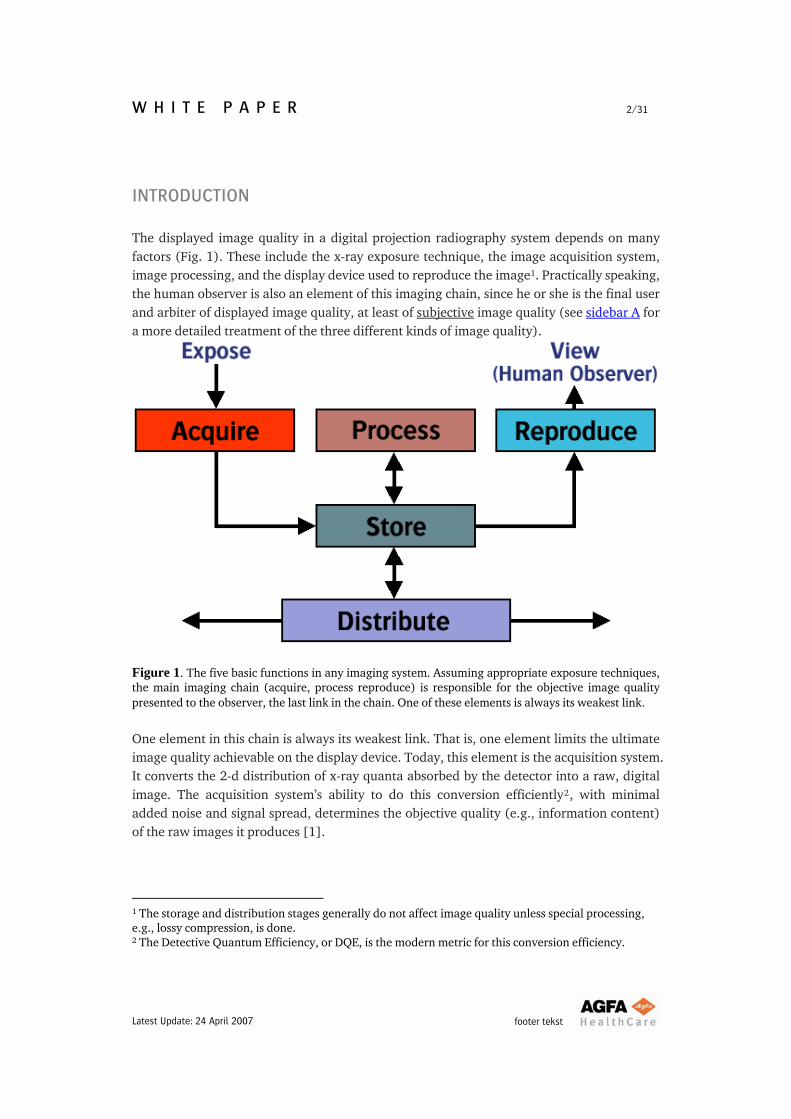
INTRODUCTION The displayed image quality in a digital projection radiography system depends on many factors (Fig. 1). These include the x-ray exposure technique, the image acquisition system, image processing, and the display device used to reproduce the image1. Practically speaking, the human observer is also an element of this imaging chain, since he or she is the final user and arbiter of displayed image quality, at least of subjective image quality (see sidebar A for a more detailed treatment of the three different kinds of image quality).

Figure 1. The five basic functions in any imaging system. Assuming appropriate exposure techniques, the main imaging chain (acquire, process reproduce) is responsible for the objective image quality presented to the observer, the last link in the chain. One of these elements is always its weakest link. One element in this chain is always its weakest link. That is, one element limits the ultimate image quality achievable on the display device. Today, this element is the acquisition system. It converts the 2-d distribution of x-ray quanta absorbed by the detector into a raw, digital image. The acquisition system’s ability to do this conversion efficiently2, with minimal added noise and signal spread, determines the objective quality (e.g., information content) of the raw images it produces [1].

1 The storage and distribution stages generally do not affect image quality unless special processing, e.g., lossy compression, is done. 2 The Detective Quantum Efficiency, or DQE, is the modern metric for this conversion efficiency.

footer tekst Latest Update: 24 April 2007


Then, the image processing and display stages must make as much as possible out of this imperfect input for human interpretation.3 Clearly, if the relevant clinical details are not captured adequately during acquisition, image processing and reproduction will not recover or display them later. However, image acquisition systems continue to improve, and the gap between real and ideal detectors4 is narrowing. At some point, the acquisition stage may no longer be the link that limits the achievable image quality. Differences in “raw” image quality between different acquisition systems will gradually decrease, and the focus of attention will shift to other elements in the imaging chain. Perhaps it is the display sub-system that will limit ultimate system performance? Certainly, the dynamic range of modern digital acquisition devices is often far greater than that of available displays. However, the dynamic range of a given radiographic image is generally not. Therefore, proper mapping of the raw image to the display dynamic range (see the tutorial on the Role of Image Processing on the Musica2 CD) can usually resolve any dynamic range mismatch. In addition, display devices, such as laser or thermal printers, and CRTs or LCD5 monitors, continue to improve. Display matrix sizes, grayscale bit depths and modern output quality-control tools (e.g., DICOM Presentation State, Grayscale Standard Display Function) ensure that displays do not impose any major limitations on overall system image quality (i.e., they are not the weak link). Interestingly, many researchers point to the human observer as the weak link in the imaging chain. There is, in fact, considerable evidence that errors in diagnostic performance (in particular, false negatives) are due not to inadequate capture, processing or display, but to observer failure [2, 3]. The radiology (and medico-legal) literature is full of examples where the missed pathology was actually present on the image, and even on prior images acquired long before the correct diagnosis was finally made. These failures can occur during different phases of the diagnostic process [4]:

Scanning: failure to look at or see the target during image viewing Detection/recognition: failure to register a scanned target as significant Interpretation: incorrect identification of a detected target Decision-making: incorrect recommendation despite correct interpretation

3 This monograph addresses only human vision. Machine vision, for example, Computer-Aided Detection and Diagnosis, or CAD, is beyond the scope of this discussion. 4 The ideal detector has a Detective Quantum Efficiency (DQE) of 1.0 5 CRT = Cathode Ray Tube; LCD = Liquid-Crystal Display



There is still much research going on today to model real observers, and to develop methods that will decrease the probability that an observer will fail in a diagnostic task [2]. Image processing could be one of those methods. The goal of much of medical image processing over the past several decades has been to find techniques that increase the visibility or conspicuity (loosely, “detail contrast”) of subtle, easily overlooked structures and, thereby, hopefully, to improve observer performance and patient care. However, image processing is a two-edged sword. Done poorly, it can completely destroy the hard work and investment that went into developing the acquisition and display subsystems. In other words, it can become the weak link in the imaging chain. Done well, it can extract as much information as possible from an acquired image, and present it in a diagnostically optimized way to the observer. Thus, image processing is, and will remain, a critical element in the digital radiographic imaging chain.

AGFA AND IMAGE PROCESSING Agfa has been at the forefront of medical image processing for well over a decade. MUSICATM, Agfa’s first medical image optimization technique, was introduced commercially in the early 1990s [5], and is still considered state-of-the-art today! It uses a multi-scale, layered representation of an image (more on this below) that enables simple and precise control over many aspects of the image “look.” Interestingly, other manufacturers of radiographic imaging systems have now moved, or are currently moving, to the same multi-scale image processing approach pioneered by Agfa in the medical field [6, 7]. However, Agfa’s innovation in image processing doesn’t stop with MUSICA.

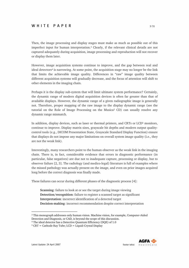
Figure 2. In current, state-of-the-art IP software for CR/DR, external user input is required in order to set the image processing parameters that produce an optimized output image. One shortcoming of all commercial image processing techniques used in digital projection radiography today, including MUSICA, is that they require additional information about the image in order to perform correctly (Fig. 2). Typically, a user must enter this information



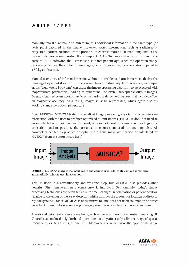
manually into the system. At a minimum, this additional information is the exam type (or body part) captured in the image. However, other information, such as radiographic projection, patient position, or the presence of contrast material or metal implants in the image is also sometimes needed. For example, in Agfa’s Pediatric software, an add-on to the basic MUSICA software, the user must also enter patient age, since the optimum image processing can be different for different age groups (for example, for a neonate compared to a 50 kg adolescent). Manual user entry of information is not without its problems. Extra input steps during the imaging of a patient slow down workflow and lower productivity. More seriously, user input errors (e.g., wrong body part) can cause the image processing algorithm to be executed with inappropriate parameters, leading to suboptimal, or even unacceptable output images. Diagnostically relevant details may become harder to detect, with a potential negative effect on diagnostic accuracy. As a result, images must be reprocessed, which again disrupts workflow and slows down patient care. Enter MUSICA2. MUSICA2 is the first medical image processing algorithm that requires no interaction with the user to produce optimized output images (Fig. 3). It does not need to know which body part has been imaged; it does not need to know about radiographic projection, patient position, the presence of contrast material, or anything else. All parameters needed to produce an optimized output image are derived or calculated by MUSICA2 from the input image itself.

Figure 3. MUSICA2 analyzes the input image and derives or calculates algorithmic parameters automatically, without user intervention. This, in itself, is a revolutionary and welcome step, but MUSICA2 also provides other benefits. First, image-to-image consistency is improved. For example, today’s image processing techniques are often sensitive to small changes in collimation or patient position relative to the edges of the x-ray detector (which changes the amount or location of direct x-ray background). Since MUSICA2 is not sensitive to, and does not need collimation or direct x-ray background information, output image presentation can be much more consistent. Traditional detail-enhancement methods, such as linear and nonlinear unsharp masking [8, 9], are based on local neighborhood operations, so they affect only a limited range of spatial frequencies, or detail sizes, at one time. Moreover, the selection of the appropriate range



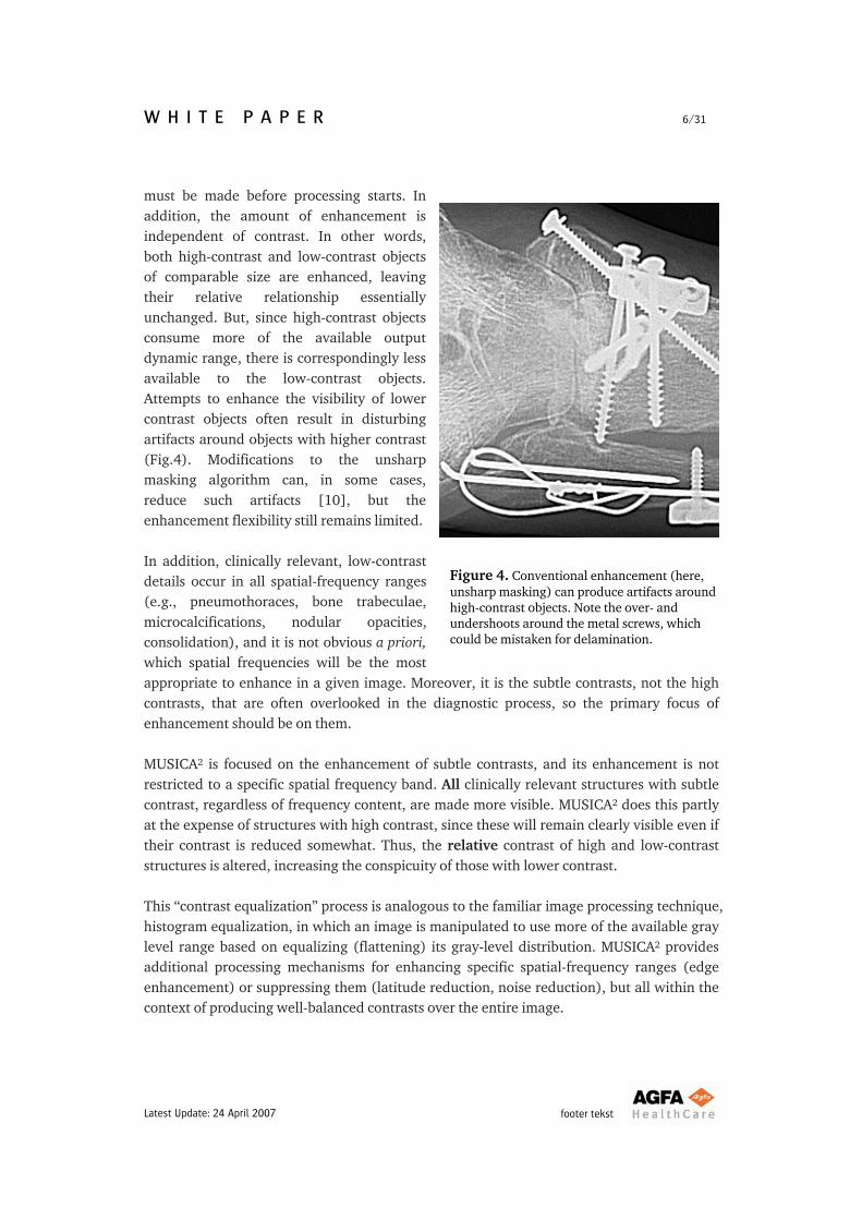
must be made before processing starts. In addition, the amount of enhancement is independent of contrast. In other words, both high-contrast and low-contrast objects of comparable size are enhanced, leaving their relative relationship essentially unchanged. But, since high-contrast objects consume more of the available output dynamic range, there is correspondingly less available to the low-contrast objects. Attempts to enhance the visibility of lower contrast objects often result in disturbing artifacts around objects with higher contrast (Fig.4). Modifications to the unsharp masking algorithm can, in some cases, reduce such artifacts [10], but the enhancement flexibility still remains limited. In addition, clinically relevant, low-contrast details occur in all spatial-frequency ranges (e.g., pneumothoraces, bone trabeculae, microcalcifications, nodular opacities, consolidation), and it is not obvious a priori, which spatial frequencies will be the most appropriate to enhance in a given image. Moreover, it is the subtle contrasts, not the high contrasts, that are often overlooked in the diagnostic process, so the primary focus of enhancement should be on them.

Figure 4. Conventional enhancement (here, unsharp masking) can produce artifacts around high-contrast objects. Note the over- and undershoots around the metal screws, which could be mistaken for delamination.

MUSICA2 is focused on the enhancement of subtle contrasts, and its enhancement is not restricted to a specific spatial frequency band. All clinically relevant structures with subtle contrast, regardless of frequency content, are made more visible. MUSICA2 does this partly at the expense of structures with high contrast, since these will remain clearly visible even if their contrast is reduced somewhat. Thus, the relative contrast of high and low-contrast structures is altered, increasing the conspicuity of those with lower contrast. This “contrast equalization” process is analogous to the familiar image processing technique, histogram equalization, in which an image is manipulated to use more of the available gray level range based on equalizing (flattening) its gray-level distribution. MUSICA2 provides additional processing mechanisms for enhancing specific spatial-frequency ranges (edge enhancement) or suppressing them (latitude reduction, noise reduction), but all within the context of producing well-balanced contrasts over the entire image.



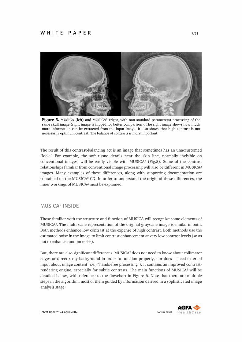
Figure 5. MUSICA (left) and MUSICA2 (right, with non standard parameters) processing of the same skull image (right image is flipped for better comparison). The right image shows how much more information can be extracted from the input image. It also shows that high contrast is not necessarily optimum contrast. The balance of contrasts is more important.

The result of this contrast-balancing act is an image that sometimes has an unaccustomed “look.” For example, the soft tissue details near the skin line, normally invisible on conventional images, will be easily visible with MUSICA2 (Fig.5). Some of the contrast relationships familiar from conventional image processing will also be different in MUSICA2 images. Many examples of these differences, along with supporting documentation are contained on the MUSICA2 CD. In order to understand the origin of these differences, the inner workings of MUSICA2 must be explained.

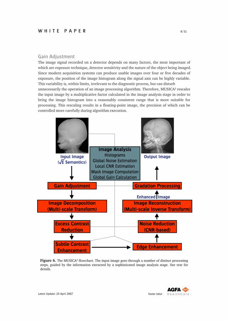
MUSICA2 INSIDE Those familiar with the structure and function of MUSICA will recognize some elements of MUSICA2. The multi-scale representation of the original grayscale image is similar in both. Both methods enhance low contrast at the expense of high contrast. Both methods use the estimated noise in the image to limit contrast enhancement at very low contrast levels (so as not to enhance random noise). But, there are also significant differences. MUSICA2 does not need to know about collimator edges or direct x-ray background in order to function properly, nor does it need external input about image content (i.e., “hands-free processing”). It contains an improved contrast-rendering engine, especially for subtle contrasts. The main functions of MUSICA2 will be detailed below, with reference to the flowchart in Figure 6. Note that there are multiple steps in the algorithm, most of them guided by information derived in a sophisticated image analysis stage.



Gain Adjustment The image signal recorded on a detector depends on many factors, the most important of which are exposure technique, detector sensitivity and the nature of the object being imaged. Since modern acquisition systems can produce usable images over four or five decades of exposure, the position of the image histogram along the signal axis can be highly variable. This variability is, within limits, irrelevant to the diagnostic process, but can disturb unnecessarily the operation of an image processing algorithm. Therefore, MUSICA2 rescales the input image by a multiplicative factor calculated in the image analysis stage in order to bring the image histogram into a reasonably consistent range that is more suitable for processing. This rescaling results in a floating-point image, the precision of which can be controlled more carefully during algorithm execution.

Figure 6. The MUSICA2 flowchart. The input image goes through a number of distinct processing steps, guided by the information extracted by a sophisticated image analysis stage. See text for details.



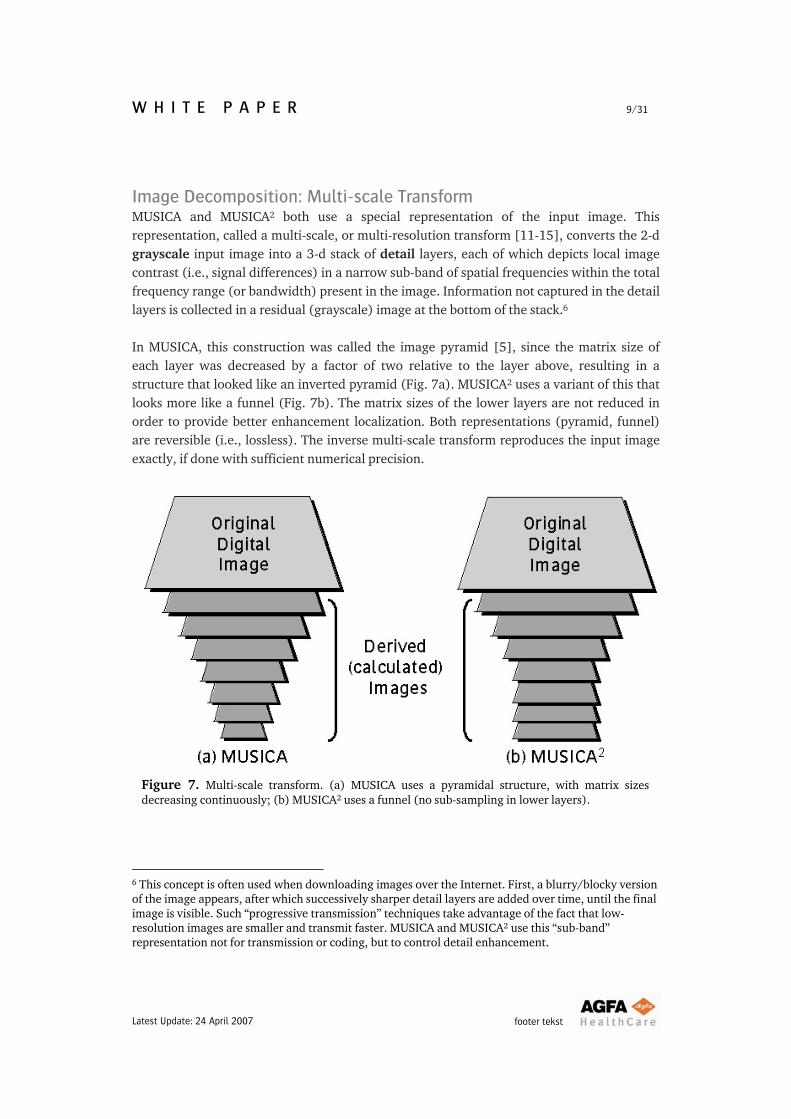
Image Decomposition: Multi-scale Transform MUSICA and MUSICA2 both use a special representation of the input image. This representation, called a multi-scale, or multi-resolution transform [11-15], converts the 2-d grayscale input image into a 3-d stack of detail layers, each of which depicts local image contrast (i.e., signal differences) in a narrow sub-band of spatial frequencies within the total frequency range (or bandwidth) present in the image. Information not captured in the detail layers is collected in a residual (grayscale) image at the bottom of the stack.6 In MUSICA, this construction was called the image pyramid [5], since the matrix size of each layer was decreased by a factor of two relative to the layer above, resulting in a structure that looked like an inverted pyramid (Fig. 7a). MUSICA2 uses a variant of this that looks more like a funnel (Fig. 7b). The matrix sizes of the lower layers are not reduced in order to provide better enhancement localization. Both representations (pyramid, funnel) are reversible (i.e., lossless). The inverse multi-scale transform reproduces the input image exactly, if done with sufficient numerical precision.

Figure 7. Multi-scale transform. (a) MUSICA uses a pyramidal structure, with matrix sizes decreasing continuously; (b) MUSICA2 uses a funnel (no sub-sampling in lower layers).

6 This concept is often used when downloading images over the Internet. First, a blurry/blocky version of the image appears, after which successively sharper detail layers are added over time, until the final image is visible. Such “progressive transmission” techniques take advantage of the fact that low-resolution images are smaller and transmit faster. MUSICA and MUSICA2 use this “sub-band” representation not for transmission or coding, but to control detail enhancement.



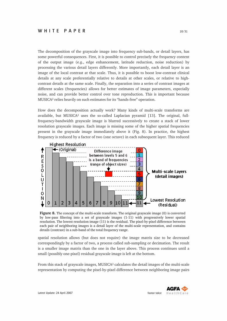
The decomposition of the grayscale image into frequency sub-bands, or detail layers, has some powerful consequences. First, it is possible to control precisely the frequency content of the output image (e.g., edge enhancement, latitude reduction, noise reduction) by processing the various detail layers differently. More importantly, each detail layer is an image of the local contrast at that scale. Thus, it is possible to boost low-contrast clinical details at any scale preferentially relative to details at other scales, or relative to high-contrast details at the same scale. Finally, the separation into a series of contrast images at different scales (frequencies) allows for better estimates of image parameters, especially noise, and can provide better control over tone reproduction. This is important because MUSICA2 relies heavily on such estimates for its “hands-free” operation. How does the decomposition actually work? Many kinds of multi-scale transforms are available, but MUSICA2 uses the so-called Laplacian pyramid [13]. The original, full-frequency-bandwidth grayscale image is blurred successively to create a stack of lower resolution grayscale images. Each image is missing some of the higher spatial frequencies present in the grayscale image immediately above it (Fig. 8). In practice, the highest frequency is reduced by a factor of two (one octave) in each subsequent layer. This reduced

spatial resolution allows (but does not require) the image matrix size to be decreased correspondingly by a factor of two, a process called sub-sampling or decimation. The result is a smaller image matrix than the one in the layer above. This process continues until a small (possibly one-pixel) residual grayscale image is left at the bottom.

Figure 8. The concept of the multi-scale transform. The original grayscale image (0) is converted by low-pass filtering into a set of grayscale images (1-11) with progressively lower spatial resolution. The lowest resolution image (11) is the residual. The pixel-by-pixel difference between each pair of neighboring images is a detail layer of the multi-scale representation, and contains details (contrast) in a sub-band of the total frequency range.

From this stack of grayscale images, MUSICA2 calculates the detail images of the multi-scale representation by computing the pixel-by-pixel difference between neighboring image pairs



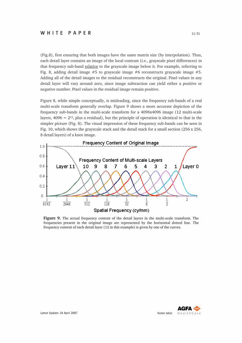
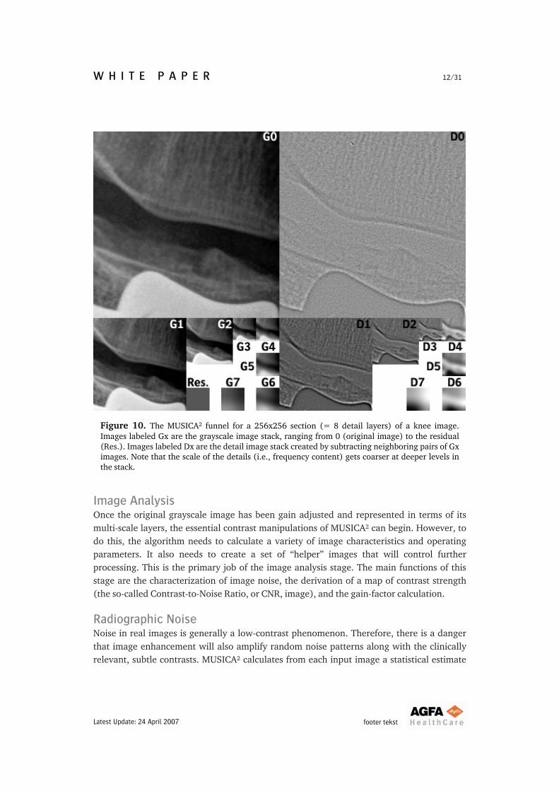
(Fig.8), first ensuring that both images have the same matrix size (by interpolation). Thus, each detail layer contains an image of the local contrast (i.e., grayscale pixel differences) in that frequency sub-band relative to the grayscale image below it. For example, referring to Fig. 8, adding detail image #5 to grayscale image #6 reconstructs grayscale image #5. Adding all of the detail images to the residual reconstructs the original. Pixel values in any detail layer will vary around zero, since image subtraction can yield either a positive or negative number. Pixel values in the residual image remain positive. Figure 8, while simple conceptually, is misleading, since the frequency sub-bands of a real multi-scale transform generally overlap. Figure 9 shows a more accurate depiction of the frequency sub-bands in the multi-scale transform for a 4096x4096 image (12 multi-scale layers, 4096 = 212, plus a residual), but the principle of operation is identical to that in the simpler picture (Fig. 8). The visual impression of these frequency sub-bands can be seen in Fig. 10, which shows the grayscale stack and the detail stack for a small section (256 x 256, 8 detail layers) of a knee image.

Figure 9. The actual frequency content of the detail layers in the multi-scale transform. The frequencies present in the original image are represented by the horizontal dotted line. The frequency content of each detail layer (12 in this example) is given by one of the curves.



Figure 10. The MUSICA2 funnel for a 256x256 section (= 8 detail layers) of a knee image. Images labeled Gx are the grayscale image stack, ranging from 0 (original image) to the residual (Res.). Images labeled Dx are the detail image stack created by subtracting neighboring pairs of Gx images. Note that the scale of the details (i.e., frequency content) gets coarser at deeper levels in the stack.

Image Analysis Once the original grayscale image has been gain adjusted and represented in terms of its multi-scale layers, the essential contrast manipulations of MUSICA2 can begin. However, to do this, the algorithm needs to calculate a variety of image characteristics and operating parameters. It also needs to create a set of “helper” images that will control further processing. This is the primary job of the image analysis stage. The main functions of this stage are the characterization of image noise, the derivation of a map of contrast strength (the so-called Contrast-to-Noise Ratio, or CNR, image), and the gain-factor calculation. Radiographic Noise Noise in real images is generally a low-contrast phenomenon. Therefore, there is a danger that image enhancement will also amplify random noise patterns along with the clinically relevant, subtle contrasts. MUSICA2 calculates from each input image a statistical estimate



of the noise level, which it uses to help distinguish subtle, clinical contrasts from noisy areas containing no usable information. Noise in radiographic images comes from several sources, the largest of which is (or, at least, should be) the quantum noise inherent in the x-ray exposure.7 In such a quantum-limited system, the magnitude of the noise (characterized by its standard deviation, σ) is related to the average exposure level [1]. Designating N as the average number of x-ray quanta absorbed by the detector per unit area (this signal, N, is proportional to exposure), the mean noise amplitude is:

N=σ This equation says that the noise increases with signal (or exposure).8 However, it does not increase as rapidly as the signal (which is linear in exposure). As a result, the signal-to-noise ratio, or SNR, improves with increasing exposure:

NN

NNNoiseSignalSNR ====

σ

Because radiographic physics naturally entails this square-root relationship between exposure and noise, Agfa has incorporated it into its Computed Radiography (CR) systems. The output gray levels of Agfa CR systems represent (i.e., are quantized as) the square root of the exposure to the image plate. The result is a practically uniform noise level over the entire image, independent of local exposure. This is a significant advantage in estimating noise and dose. Other manufacturers use different quantization schemes during acquisition, most often “log E.” In this scheme, the acquired signal is proportional to the logarithm of the exposure, rather than to the square root. MUSICA2 expects to see at its input an image quantized with square-root semantics (as indicated in Fig. 6). If this is not the case, the image signal values must be converted before processing. For further information on square-root semantics, see sidebar B. Noise and MUSICA2

Image noise can exist at a variety of spatial frequencies, but it is most disturbing to human observers at higher frequencies. Therefore, MUSICA2 uses only the finest detail layer (Layer

7 While the acquisition system also adds noise to the raw image, its effect must remain as small as possible over the range of clinical exposures in order to maintain high DQE. 8 Commonly heard statements to the effect that “noise decreases at high exposures” are patently false. The reason that images made at higher exposures look smoother and less noisy is that the signal-to-noise ratio, which is what drives visual perception, increases with exposure.



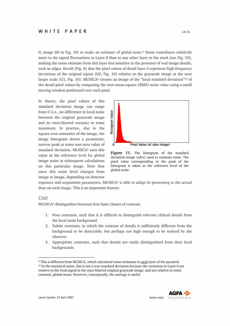
0; image D0 in Fig. 10) to make an estimate of global noise.9 Noise contributes relatively more to the signal fluctuations in Layer 0 than to any other layer in the stack (see Fig. 10), making the noise estimate from this layer less sensitive to the presence of real image details, such as edges. Recall (Fig. 8) that the pixel values of detail layer 0 represent high-frequency deviations of the original signal (G0, Fig. 10) relative to the grayscale image at the next larger scale (G1, Fig. 10). MUSICA2 creates an image of the “local standard deviation”10 of the detail-pixel values by computing the root-mean-square (RMS) noise value using a small moving window positioned over each pixel. In theory, the pixel values of this standard deviation image can range from 0 (i.e., no difference in local noise between the original grayscale image and its once-blurred version) to some maximum. In practice, due to the square-root semantics of the image, the image histogram shows a prominent, narrow peak at some non-zero value of standard deviation. MUSICA2 uses this value as the reference level for global image noise in subsequent calculations on this particular image. Note that since this noise level changes from image to image, depending on detector exposure and acquisition parameters, MUSICA2 is able to adapt its processing to the actual dose on each image. This is an important feature.

Figure 11. The histogram of the standard deviation image (sdev) used to estimate noise. The pixel value corresponding to the peak of the histogram is taken as the reference level of the global noise.

CNR MUSICA2 distinguishes between four basic classes of contrast:

1. Poor contrasts, such that it is difficult to distinguish relevant clinical details from the local noise background

2. Subtle contrasts, in which the contrast of details is sufficiently different from the background to be detectable, but perhaps not high enough to be noticed by the observer

3. Appropriate contrasts, such that details are easily distinguished from their local backgrounds

9 This is different from MUSICA, which calculated noise estimates in each layer of the pyramid. 10 In the statistical sense, this is not a true standard deviation because the variations in Layer 0 are relative to the local signal in the once-blurred original grayscale image, and not relative to some constant, global mean. However, conceptually, the analogy is useful.



4. Excessive contrasts, in which structures occupy a disproportionate fraction of the available dynamic range and, therefore, leave less dynamic range for other image details.

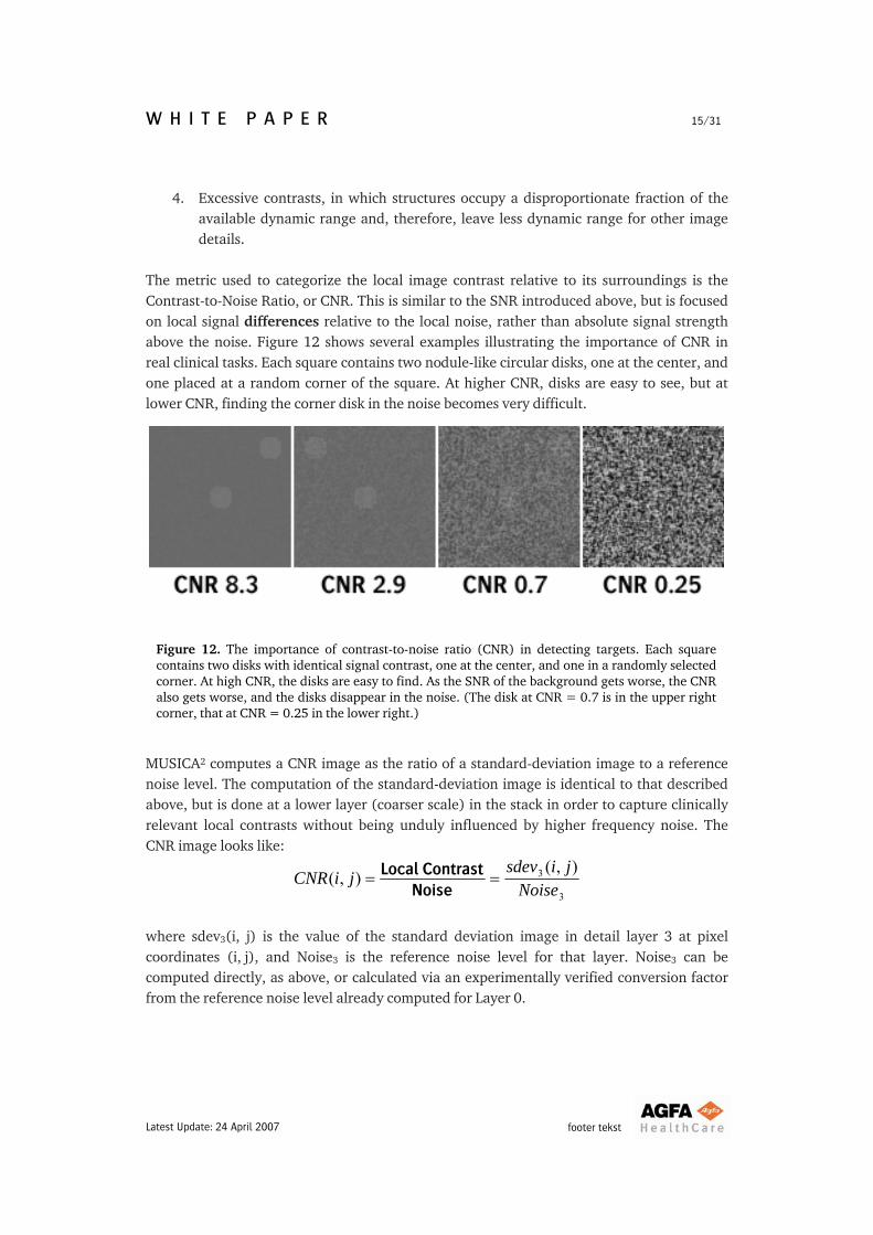
The metric used to categorize the local image contrast relative to its surroundings is the Contrast-to-Noise Ratio, or CNR. This is similar to the SNR introduced above, but is focused on local signal differences relative to the local noise, rather than absolute signal strength above the noise. Figure 12 shows several examples illustrating the importance of CNR in real clinical tasks. Each square contains two nodule-like circular disks, one at the center, and one placed at a random corner of the square. At higher CNR, disks are easy to see, but at lower CNR, finding the corner disk in the noise becomes very difficult.

Figure 12. The importance of contrast-to-noise ratio (CNR) in detecting targets. Each square contains two disks with identical signal contrast, one at the center, and one in a randomly selected corner. At high CNR, the disks are easy to find. As the SNR of the background gets worse, the CNR also gets worse, and the disks disappear in the noise. (The disk at CNR = 0.7 is in the upper right corner, that at CNR = 0.25 in the lower right.)

MUSICA2 computes a CNR image as the ratio of a standard-deviation image to a reference noise level. The computation of the standard-deviation image is identical to that described above, but is done at a lower layer (coarser scale) in the stack in order to capture clinically relevant local contrasts without being unduly influenced by higher frequency noise. The CNR image looks like:

3

3 ),(),(

Noisejisdev

jiCNR ==Noise

Contrast Local

where sdev3(i, j) is the value of the standard deviation image in detail layer 3 at pixel coordinates (i, j), and Noise3 is the reference noise level for that layer. Noise3 can be computed directly, as above, or calculated via an experimentally verified conversion factor from the reference noise level already computed for Layer 0.



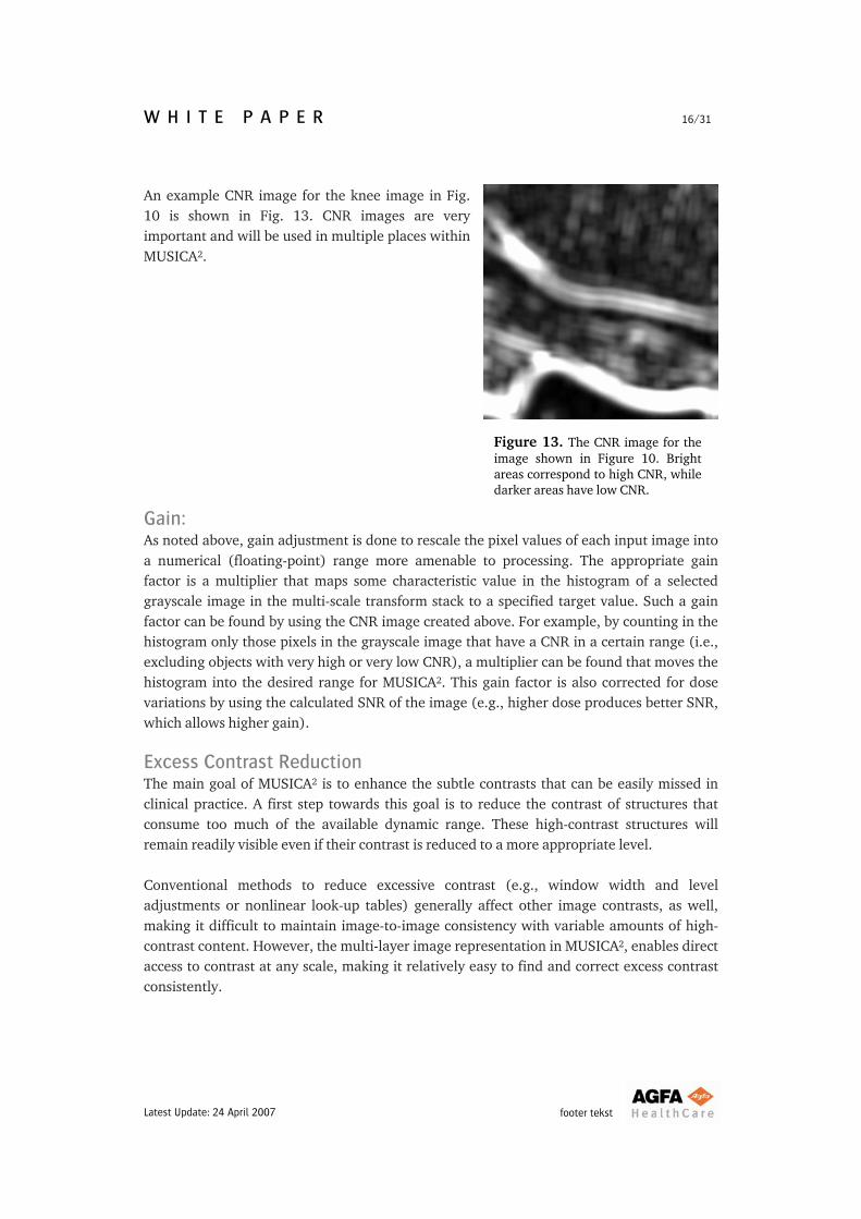
An example CNR image for the knee image in Fig. 10 is shown in Fig. 13. CNR images are very important and will be used in multiple places within MUSICA2. Figure 13. The CNR image for the

image shown in Figure 10. Bright areas correspond to high CNR, while darker areas have low CNR.

Gain: As noted above, gain adjustment is done to rescale the pixel values of each input image into a numerical (floating-point) range more amenable to processing. The appropriate gain factor is a multiplier that maps some characteristic value in the histogram of a selected grayscale image in the multi-scale transform stack to a specified target value. Such a gain factor can be found by using the CNR image created above. For example, by counting in the histogram only those pixels in the grayscale image that have a CNR in a certain range (i.e., excluding objects with very high or very low CNR), a multiplier can be found that moves the histogram into the desired range for MUSICA2. This gain factor is also corrected for dose variations by using the calculated SNR of the image (e.g., higher dose produces better SNR, which allows higher gain). Excess Contrast Reduction The main goal of MUSICA2 is to enhance the subtle contrasts that can be easily missed in clinical practice. A first step towards this goal is to reduce the contrast of structures that consume too much of the available dynamic range. These high-contrast structures will remain readily visible even if their contrast is reduced to a more appropriate level. Conventional methods to reduce excessive contrast (e.g., window width and level adjustments or nonlinear look-up tables) generally affect other image contrasts, as well, making it difficult to maintain image-to-image consistency with variable amounts of high-contrast content. However, the multi-layer image representation in MUSICA2, enables direct access to contrast at any scale, making it relatively easy to find and correct excess contrast consistently.



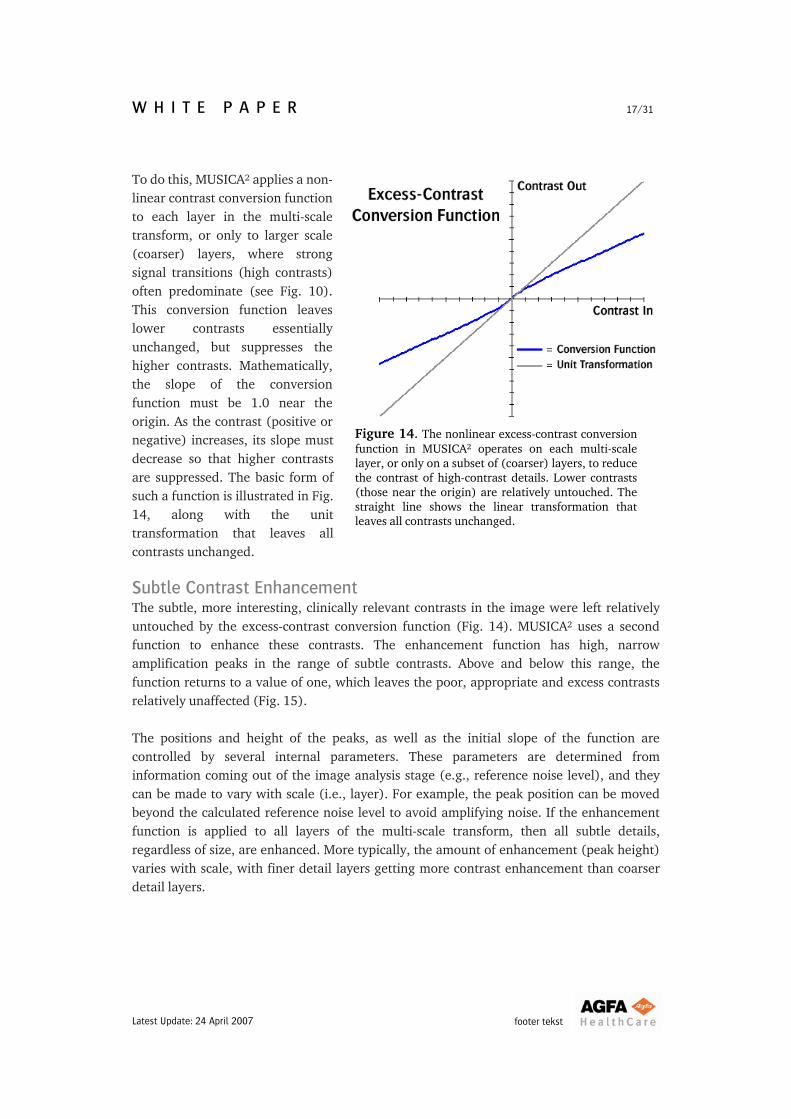
To do this, MUSICA2 applies a non-linear contrast conversion function to each layer in the multi-scaletransform, or only to larger scale (coarser) layers, where strong signal transitions (high contrasts) often predominate (see Fig. 10). This conversion function leaves lower contrasts essentially unchanged, but suppresses the higher contrasts. Mathematically, the slope of the conversion function must be 1.0 near the origin. As the contrast (positive or negative) increases, its slope must decrease so that higher contrasts are suppressed. The basic form of such a function is illustrated in Fig. 14, along with the unit transformation that leaves all contrasts unchanged.

Figure 14. The nonlinear excess-contrast conversion function in MUSICA2 operates on each multi-scale layer, or only on a subset of (coarser) layers, to reduce the contrast of high-contrast details. Lower contrasts (those near the origin) are relatively untouched. The straight line shows the linear transformation that leaves all contrasts unchanged.

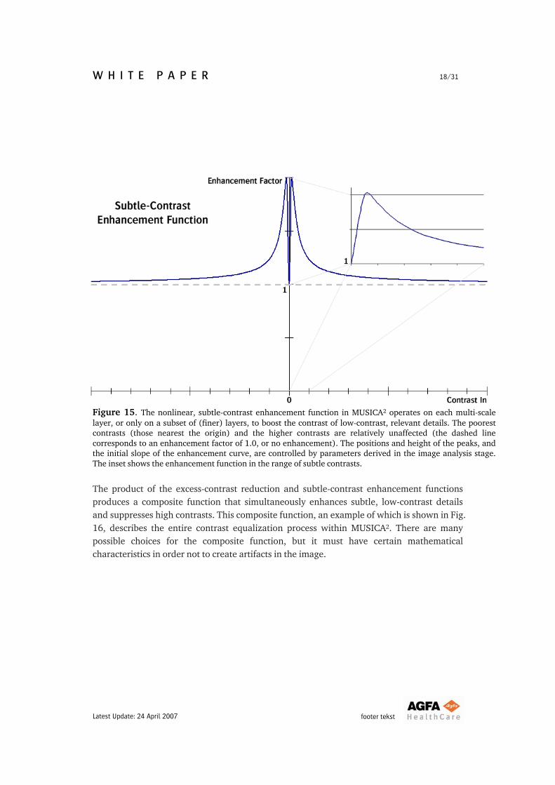
Subtle Contrast Enhancement The subtle, more interesting, clinically relevant contrasts in the image were left relatively untouched by the excess-contrast conversion function (Fig. 14). MUSICA2 uses a second function to enhance these contrasts. The enhancement function has high, narrow amplification peaks in the range of subtle contrasts. Above and below this range, the function returns to a value of one, which leaves the poor, appropriate and excess contrasts relatively unaffected (Fig. 15). The positions and height of the peaks, as well as the initial slope of the function are controlled by several internal parameters. These parameters are determined from information coming out of the image analysis stage (e.g., reference noise level), and they can be made to vary with scale (i.e., layer). For example, the peak position can be moved beyond the calculated reference noise level to avoid amplifying noise. If the enhancement function is applied to all layers of the multi-scale transform, then all subtle details, regardless of size, are enhanced. More typically, the amount of enhancement (peak height) varies with scale, with finer detail layers getting more contrast enhancement than coarser detail layers.



Figure 15. The nonlinear, subtle-contrast enhancement function in MUSICA2 operates on each multi-scale layer, or only on a subset of (finer) layers, to boost the contrast of low-contrast, relevant details. The poorest contrasts (those nearest the origin) and the higher contrasts are relatively unaffected (the dashed line corresponds to an enhancement factor of 1.0, or no enhancement). The positions and height of the peaks, and the initial slope of the enhancement curve, are controlled by parameters derived in the image analysis stage. The inset shows the enhancement function in the range of subtle contrasts. The product of the excess-contrast reduction and subtle-contrast enhancement functions produces a composite function that simultaneously enhances subtle, low-contrast details and suppresses high contrasts. This composite function, an example of which is shown in Fig. 16, describes the entire contrast equalization process within MUSICA2. There are many possible choices for the composite function, but it must have certain mathematical characteristics in order not to create artifacts in the image.



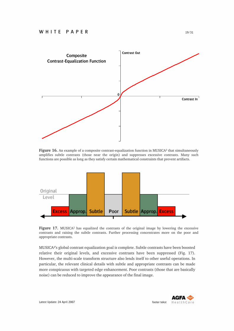
Figure 16. An example of a composite contrast-equalization function in MUSICA2 that simultaneously amplifies subtle contrasts (those near the origin) and suppresses excessive contrasts. Many such functions are possible as long as they satisfy certain mathematical constraints that prevent artifacts.

Figure 17. MUSICA2 has equalized the contrasts of the original image by lowering the excessive contrasts and raising the subtle contrasts. Further processing concentrates more on the poor and appropriate contrasts. MUSICA2’s global contrast equalization goal is complete. Subtle contrasts have been boosted relative their original levels, and excessive contrasts have been suppressed (Fig. 17). However, the multi-scale transform structure also lends itself to other useful operations. In particular, the relevant clinical details with subtle and appropriate contrasts can be made more conspicuous with targeted edge enhancement. Poor contrasts (those that are basically noise) can be reduced to improve the appearance of the final image.



Edge Enhancement Images appear sharper when more emphasis is placed on higher spatial frequencies. Since various frequency sub-bands are directly accessible as layers of the multi-scale representation (Figs. 8, 9), edge enhancement in MUSICA2 is straightforward and easily controlled. One simple method, which is built into the algorithm, is to multiply each detail layer by a different weighting factor (this is also the technique used in MUSICA). These weighting factors are greater than one for finer resolution scales, and decrease to one, and remain at one, at mid- to coarser scales. In this case, all contrasts in a given layer are multiplied by the same weighting factor. The preferred approach in MUSICA2 is to vary as a function of scale (layer) the parameter that controls the height of the peaks in the subtle contrast enhancement function (Fig. 15). The peaks are given maximum height in Layer 0, and their height decreases continuously until it reaches some constant value at mid- to coarser scales. This approach has several advantages. One is that edge enhancement is done simultaneously with the enhancement of subtle contrast, saving processing steps. In addition, the position of the peaks in the subtle contrast enhancement function has already been tuned to exclude contrast comparable to or lower than the reference noise level. This means that edge enhancement takes place only in the range of relevant subtle contrasts, and not in the noise. Also, large contrasts at finer scales (i.e., strong edges) are not further enhanced since the subtle contrast enhancement applies only at lower contrasts. Noise Reduction The human eye is more sensitive to noise in subtle areas of an image than in busy areas. Thus, any noise enhanced by the contrast equalization process may detract from the final image. Although desirable, noise-reduction processing can also introduce artifacts into the image. Therefore, noise reduction is usually applied sparingly, if at all. In MUSICA, noise reduction was addressed by calculating at each scale/layer a local standard deviation for each pixel. This pixel standard deviation was compared to the calculated noise level at the same scale, and the pixel was attenuated if its value was too close to the noise level (i.e., contained no discernable image detail). MUSICA2 takes a different approach. It uses a slightly filtered version of the CNR image calculated in the image analysis stage to control the noise reduction process in each detail layer in which it will be done. The basic idea is that pixels in the participating detail layers are evaluated, and attenuated, based on the corresponding pixel in the CNR image. If the CNR of a pixel is less than some minimum value, the pixel is multiplied by a constant attenuation coefficient less than one. This is because it is likely that the pixel belongs to a relatively homogeneous area where noise would be visually disturbing. Conversely, if the pixel CNR is greater than some maximum value, it is multiplied by a constant “attenuation”



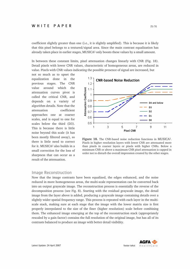
coefficient slightly greater than one (i.e., it is slightly amplified). This is because it is likely that this pixel belongs to a textured/signal area. Since the main contrast equalization has already taken place in earlier stages, MUSICA2 only boosts these values by a small amount. In between these constant limits, pixel attenuation changes linearly with CNR (Fig. 18). Detail pixels with lower CNR values, characteristic of homogeneous areas, are reduced in value. Pixels with CNR values indicating the possible presence of signal are increased, but

not so much as to upset the equalization done in the previous stages. The CNR value around which the attenuation curves pivot is called the critical CNR, and depends on a variety of algorithm details. Note that the attenuation coefficient approaches one at coarser scales, and is equal to one for scales below the third (D3). This is because there is little noise beyond this scale (it has been mostly filtered away), so there is little need to correct for it. MUSICA2 also builds in a small correction for the loss of sharpness that can occur as a result of the attenuation.

Figure 18. The CNR-based noise reduction functions in MUSICA2. Pixels in higher resolution layers with lower CNR are attenuated more than pixels in coarser layers or pixels with higher CNRs. Below a minimum CNR or above a maximum CNR pixel attenuation is capped in order not to disturb the overall impression created by the other stages.

Image Reconstruction Now that the image contrasts have been equalized, the edges enhanced, and the noise reduced in more homogeneous areas, the multi-scale representation can be converted back into an output grayscale image. The reconstruction process is essentially the reverse of the decomposition process (see Fig. 8). Starting with the residual grayscale image, the detail image from the layer above is added, producing a grayscale image containing details over a slightly wider spatial frequency range. This process is repeated with each layer in the multi-scale stack, making sure at each stage that the image with the lower matrix size is first properly interpolated to the size of the finer (higher resolution) scale before combining them. The enhanced image emerging at the top of the reconstruction stack (appropriately rescaled by a gain factor) contains the full resolution of the original image, but has all of its contrasts balanced to produce an image with better detail visibility.



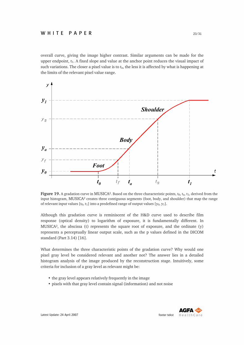
Gradation Processing While the relative contrast relationships, sharpness, and noise properties of the enhanced, reconstructed image are internally optimized, the image is not yet ready for viewing. It must first be sent through a tone reproduction curve appropriate for the display. Gradation processing, the creation of such tone reproduction curves for medical images, is an area where MUSICA2 distinguishes itself from its predecessors, including MUSICA. In particular, MUSICA2 is self-bootstrapping. It derives all the parameters needed for optimized output-image display from the input image itself. It does not need exam or projection information. It is not sensitive to, nor does it need, collimation or direct x-ray background location information to optimize tone reproduction. It produces high-quality output images even more consistently than MUSICA. Methods used to prepare an image for viewing/display range from simple linear re-scaling (window width/level) to sophisticated nonlinear techniques. MUSICA2 is actually compatible with a variety of methods. This monograph provides an overview of only one nonlinear technique that uses three characteristic points, derived from the input image histogram, to determine the shape of the complete nonlinear gradation curve. The method creates a sigmoid gradation curve from three contiguous segments: a (nonlinear) foot segment, a (nominally linear) body segment, and a (nonlinear) shoulder segment, each of which contains one of the characteristic points, denoted t0, ta and t1 (Fig.19). At the junctions between the segments, the method ensures that the values and slopes of the segments match, so as to produce a mathematically continuous curve. The two characteristic points, t0 and t1, define the range of relevant11 input gray levels that will be mapped to a pre-defined output range, denoted [y0, y1]. Input pixels with gray levels outside [t0, t1] will generally be mapped to fixed maximum or minimum output values. The third point, denoted ta, is called the anchor point. The value (ya) and slope (contrast) of the gradation curve at the anchor point are fixed for all images. This constraint buffers the gradation curve against variations caused by movement of the endpoints, and produces consistent image appearance across a broad spectrum of input images, as long as the input image histogram is mapped properly to the three points (see below). For example, if the endpoint, t0, must move lower to accommodate lighter pixels containing relevant image detail, it would tend to pull the entire gradation curve flatter, causing the overall image appearance (contrast) to flatten. If, on the other hand, it moved closer to ta because there is little relevant information at low pixel values, it would tend to increase the slope of the

11 The relevant range of input pixel values is generally a subset of the full range of available values (e.g., 0-4095 for a 12-bit input). The derivation of the relevant range is described later.



overall curve, giving the image higher contrast. Similar arguments can be made for the upper endpoint, t1. A fixed slope and value at the anchor point reduces the visual impact of such variations. The closer a pixel value is to ta, the less it is affected by what is happening at the limits of the relevant pixel value range.

Figure 19. A gradation curve in MUSICA2. Based on the three characteristic points, t0, ta, t1, derived from the input histogram, MUSICA2 creates three contiguous segments (foot, body, and shoulder) that map the range of relevant input values [t0, t1] into a predefined range of output values [y0, y1]. Although this gradation curve is reminiscent of the H&D curve used to describe film response (optical density) to logarithm of exposure, it is fundamentally different. In MUSICA2, the abscissa (t) represents the square root of exposure, and the ordinate (y) represents a perceptually linear output scale, such as the p values defined in the DICOM standard (Part 3.14) [16]. What determines the three characteristic points of the gradation curve? Why would one pixel gray level be considered relevant and another not? The answer lies in a detailed histogram analysis of the image produced by the reconstruction stage. Intuitively, some criteria for inclusion of a gray level as relevant might be:

• the gray level appears relatively frequently in the image • pixels with that gray level contain signal (information) and not noise



• pixels with that gray level are part of a coherent region of pixels that are also considered relevant.

To determine which gray levels are relevant and which are not, MUSICA2 uses a calculated figure of merit (FOM) that embodies the above conditions. This FOM uses two histograms: the full histogram of the reconstructed image, and a so-called restricted histogram that includes only pixels classified as relevant according to a certain CNR criterion. The CNR criterion excludes pixels with very low or very high CNR, in other words, homogeneous areas unlikely to contain relevant information, and areas with very strong edges unlikely to contain normal anatomical structures. Implementation of the CNR criterion is done with a binary mask image, calculated in the image analysis stage, that labels relevant pixels as TRUE and irrelevant pixels as FALSE. Only pixels labeled as TRUE are included in the restricted histogram. The FOM, which is a function of both the restricted and unrestricted histograms, peaks at some gray level, and tails off on either side. The bounds of the relevant gray level range, [t0, t1], are determined from the gray levels for which the FOM exceeds some threshold values on either side of the peak. The anchor point, ta, depends on the position of the FOM peak and a third threshold. With the three characteristic points calculated, MUSICA2 then constructs the gradation curve using functional forms for the curve shape in each segment. The result (Fig. 6) is an output image with balanced contrasts, improved sharpness, reduced noise, and a tone reproduction curve optimized for interpretation by a human observer.

THE BOTTOM LINE One of the primary goals of medical image processing research and development over the last twenty years, or so, has been to develop “intelligent” algorithms that can optimize displayed image quality consistently, with minimal or no user interaction. To say the least, this goal has been elusive. MUSICA2 is the first medical image processing algorithm with sufficient innate intelligence to perform this task. And, based on clinical comparisons to more traditional image processing techniques, it performs this task well (see other documents on this CD for more details on the clinical evaluations of MUSICA2). It should be obvious to the reader that this enhanced level of intelligence makes MUSICA2 relatively complex internally, involving a sophisticated image analysis stage, multiple processing steps, and many fixed and computed parameters. The intent of this monograph was to expose deliberately many of the more complex aspects of this next generation in order to give the reader a better understanding of what actually happens inside the “black box,” and, thereby, instill greater confidence in its results. Only with a reasonable degree of confidence can users appreciate and take full advantage of the new processing paradigm.



In practice, this increased complexity is hidden from the user, enabling him or her to focus on the diagnostic task and not on the diagnostic tool. This is as it should be. This next generation of image processing, exemplified by MUSICA2, will essentially eliminate the need for users to spend months, or even longer, tuning and optimizing image processing parameters for their specific environment, as is often the case today. Because it needs only an input image to function, MUSICA2 will produce diagnostic-quality results “out of the box.” Still, Agfa understands that sometimes there will be local image presentation preferences that vary from the default presentation. That’s why Agfa makes available its Professional Services team to train users on integrating MUSICA2 into their environment, and to conduct any necessary fine-tuning of the image presentation preferences (click on the SERVICES Tab on the MUSICA2 CD for more details). MUSICA2 represents a major advance in medical image processing. Along with automatically optimized, consistent output image quality, the advent of “hands-free” image processing can have significant implications for workflow and productivity in the clinical environment (details can be found elsewhere on this CD). A worthy successor to MUSICA, MUSICA2 demonstrates Agfa’s continued commitment to improve image processing, and to have a positive impact on the clinical, technical, operational and economic challenges of its customers.



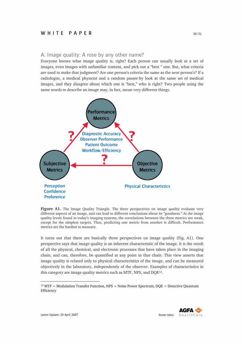
A: Image quality: A rose by any other name? Everyone knows what image quality is, right? Each person can usually look at a set of images, even images with unfamiliar content, and pick out a “best “ one. But, what criteria are used to make that judgment? Are one person’s criteria the same as the next person’s? If a radiologist, a medical physicist and a random passer-by look at the same set of medical images, and they disagree about which one is “best,” who is right? Two people using the same words to describe an image may, in fact, mean very different things.

Figure A1. The Image Quality Triangle. The three perspectives on image quality evaluate very different aspects of an image, and can lead to different conclusions about its “goodness.” At the image quality levels found in today’s imaging systems, the correlations between the three metrics are weak, except for the simplest targets. Thus, predicting one metric from another is difficult. Performance metrics are the hardest to measure. It turns out that there are basically three perspectives on image quality (Fig. A1). One perspective says that image quality is an inherent characteristic of the image. It is the result of all the physical, chemical, and electronic processes that have taken place in the imaging chain, and can, therefore, be quantified at any point in that chain. This view asserts that image quality is related only to physical characteristics of the image, and can be measured objectively in the laboratory, independently of the observer. Examples of characteristics in this category are image quality metrics such as MTF, NPS, and DQE12.

12 MTF = Modulation Transfer Function, NPS = Noise Power Spectrum, DQE = Detective Quantum Efficiency



A second view says that image quality is basically “in the eye of the beholder.” The observer’s subjective perception of the image, not the image itself, is the determinant of quality. This kind of image quality comes into play every time an observer views an image or evaluates the results of a new image processing algorithm. It is also important in determining a radiologist’s diagnostic confidence using a particular image, or imaging system. The third perspective asserts that image quality is defined by the ability of an image, or imaging system, to enable a trained observer to achieve some measure of performance for a specified task. Not only must the task-relevant details be captured, they must also be easy for an observer familiar with the task to extract and interpret. In a wider sense, this view of image quality could even include patient outcome or efficacy, as well as workflow and efficiency. One might assume that these three image quality views are related or correlated in some way. For example, an image with poor objective image quality is unlikely to create a good subjective impression, or high observer performance. As the objective image quality improves, one would also expect to see improvements in the subjective and performance-based measures. Unfortunately, except for the simplest imaging configurations, with well-characterized geometric targets in relatively uncluttered fields (i.e., not real medical images), the relationships between the three measures are, in fact, not obvious or easy to characterize. For example, the objective image quality of diagnostic imaging systems has changed dramatically since Roentgen’s discovery of x-rays in 1895 (generally increasing over time, but not monotonically). However, the diagnostic accuracy, or performance, of radiologists (at least without computer-aided detection) has remained relatively unchanged since it was first measured in the 1950s. Thus, the correlation between task performance and objective image quality, at least at the quality levels present for the last half century, appears to be weak. Moreover, significant physical (objective) image quality improvements made to screen/film systems have sometimes gone (subjectively) unnoticed on the viewbox. On rare occasions, new, subjectively preferred image display modes (e.g., black bone presentation) have actually led to lower observer performance (at least initially). The bottom line is that image quality is more complex than one might think. Image quality is not image quality. Depending on the individual, it may be based on physical, objective characteristics of the image, on qualitative, subjective impressions, or on quantitative metrics of observer performance for some diagnostic task. So, in discussions about image quality, one must be careful to know which of the three perspectives is intended. People may be using the same words, but may be talking about very different things!

Return to text.



B: Hip to be Square (Root) The creation of a digital image involves multiple steps. First, an aerial image (or image-in-space), consisting of a flux of x-ray photons in air, interacts with an x-ray detector. This interaction is generally in the form of x-ray absorption, followed by the creation within the detector of a latent image that is proportional to the absorbed x-ray energy at each point (which, in turn, is proportional to the exposure at that point). This latent image is then converted into a raw, digital image by measuring it on a regular grid of points (a process called sampling), and quantizing the measured values to a fixed number of bits (e.g., 10-14 bits for commercial CR/DR systems). The details of this quantization step vary between systems. In most commercial systems, the measured latent image values are first transformed logarithmically into an analog signal. This logarithmic analog signal is then quantized to the desired number of bits, resulting in gray levels proportional to log10 E, where E is the exposure. In other digital systems, the latent image is simply quantized linearly with more bits than will be used for the final image, and then converted digitally (via a look-up table) into a logarithmic raw image with fewer (e.g., 10-12) bits. Nonlinear conversion functions, like the logarithm, serve several purposes. First, they compress the often large dynamic range of the detector into a more manageable numerical range. They also distribute the acquired data in a manner that is more consistent with the fundamental x-ray absorption process (x-ray attenuation displays an exponential decay, so logarithmic conversion provides a more linear image of attenuation). Nonlinear conversion also matches better the nonlinear response of the human visual system (e.g., a small ∆E at low exposures produces a different response than the same ∆E at higher exposures). Agfa uses a different nonlinear quantization approach to acquisition in its CR systems. Instead of logarithmic quantization, the latent image is converted with a square-root function. The rationale for this departure from convention, as noted in the section on “Radiographic Noise,” is that the noise in an x-ray exposure is proportional to the square root of the mean signal. This is a natural consequence of the fact that x-ray quanta obey Poisson statistics (not the more familiar Gaussian statistics), in which the variance (σ2) is equal to the mean. This square-root transformation produces a raw image in which the noise is (approximately) independent of the signal, in other words, constant. The proof of this assertion is



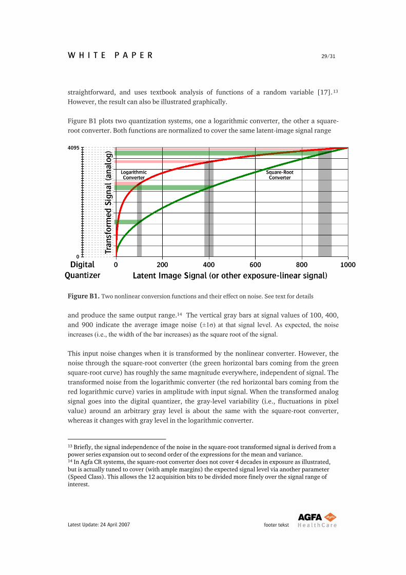
straightforward, and uses textbook analysis of functions of a random variable [17].13 However, the result can also be illustrated graphically. Figure B1 plots two quantization systems, one a logarithmic converter, the other a square-root converter. Both functions are normalized to cover the same latent-image signal range

Figure B1. Two nonlinear conversion functions and their effect on noise. See text for details and produce the same output range.14 The vertical gray bars at signal values of 100, 400, and 900 indicate the average image noise (±1σ) at that signal level. As expected, the noise increases (i.e., the width of the bar increases) as the square root of the signal. This input noise changes when it is transformed by the nonlinear converter. However, the noise through the square-root converter (the green horizontal bars coming from the green square-root curve) has roughly the same magnitude everywhere, independent of signal. The transformed noise from the logarithmic converter (the red horizontal bars coming from the red logarithmic curve) varies in amplitude with input signal. When the transformed analog signal goes into the digital quantizer, the gray-level variability (i.e., fluctuations in pixel value) around an arbitrary gray level is about the same with the square-root converter, whereas it changes with gray level in the logarithmic converter.

13 Briefly, the signal independence of the noise in the square-root transformed signal is derived from a power series expansion out to second order of the expressions for the mean and variance. 14 In Agfa CR systems, the square-root converter does not cover 4 decades in exposure as illustrated, but is actually tuned to cover (with ample margins) the expected signal level via another parameter (Speed Class). This allows the 12 acquisition bits to be divided more finely over the signal range of interest.



This noise constancy is a powerful property that allows an image processing technique like MUSICA2 to make accurate noise estimates by examining any reasonably flat (i.e., low-CNR) area within the image. These noise estimates can be used, among other things, to tune the processing to the noise content, either enhancing or suppressing local contrast based on the magnitude of the noise relative to local signals. This is more difficult, with logarithmically quantized data, since the local noise still varies nonlinearly with the signal.

Return to text. REFERENCES 1. For discussions of fundamental quantum detection issues and image quality, see, for

example: Dainty JC, Shaw R. Image Science. London: Academic Press, 1974. or Dobbins III JT. Image quality metrics for digital systems. In: Beutel J, Kundel HL, Van Metter RL, eds. Handbook of Medical Imaging, Vol.1. Physics and Psychophysics. Bellingham, WA: SPIE Press, 2000; 161-222.

2. Krupinski EA. Practical applications of perceptual research. In: Beutel J, Kundel HL, Van Metter RL, eds. Handbook of Medical Imaging, Vol.1. Bellingham, WA: SPIE Press, 2000; 895-929. (and references therein)

3. Berlin L, Berlin JW. Malpractice and radiologists in Cook County, IL: trends in 20 years of litigation. Am J Roentgen 1995; 165:781-788.

4. Kundel H, Visual search, object recognition and reader error in radiology. Proc SPIE 2004; 5372:1-11.

5. Vuylsteke P, Schoeters E. Multiscale image contrast amplification (MUSICA). Proc SPIE 1994, 2167:551-560.

6. Stahl M, Aach T, Dippel S, Digital radiography enhancement by nonlinear multiscale processing. Med Phys 2000; 27:56-65.

7. Dippel S, Stahl M, Wiemker R, Blaffert T. Multiscale contrast enhancement for radiography: Laplacian pyramid versus fast wavelet transform. IEEE Trans Med Imaging 2002; 21:343-353.

8. Cocklin ML, Gourlay AR, Jackson PH, et al. Digital processing of chest radiographs. Image and Vision Computing 1983; 1:67-78

9. Prokop M, Neitzel U, Schaefer-Prokop C. Principles of image processing in digital chest radiography. J Thorac Imaging 2003; 18:148-164.

10. Sezan MI, Tekalp AM, Schaetzing R. Automatic anatomically selective image enhancement in digital chest radiography. IEEE Trans Med Imag 1989; 8:154-162.



11. Akansu AN, Haddad RA. Multiresolution signal decomposition. New York: Academic Press, 1992; 304--306.

12. Jin Y, Fayad L, Laine AF. Contrast enhancement by multiscale adaptive histogram equalization. Proc SPIE 2001; 4478:206-213.

13. Burt PJ, Adelson EH. The Laplacian pyramid as a compact image code. IEEE Trans Comm 1983; 31:532-540.

14. Chen Z, Tao Y, Chen X. Multiresolution local contrast enhancement of x-ray images for poultry meat inspection. Appl Opt 2001; 40:1195-1200.

15. Sakellaropoulos P, Costaridou L, Panayiotakis G. A wavelet-based spatially adaptive method for mammographic contrast enhancement. Phys Med Biol 2003; 48:787-803

16. NEMA Publication PS3.14-2001. Digital imaging and communications in medicine (DICOM) Part 14: Grayscale Standard Display Function, Rosslyn, VA: National Electrical Manufacturers Association, 2001;

17. Papoulis A. Probability, Random Variables, and Stochastic Processes. New York: McGraw-Hill, 1965; 151-152.


Documents

Agfa's MUSICA2 TM Taking Image Processing to - Agfa HealthCare