1

Aggregate and Workforce Planning (Huvudplanering)

Production and Inventory Control (MPS)MIO030

The main reference for this material is the book Factory Physics by W. Hopp and M.L Spearman, McGraw-Hill, 2001.

2

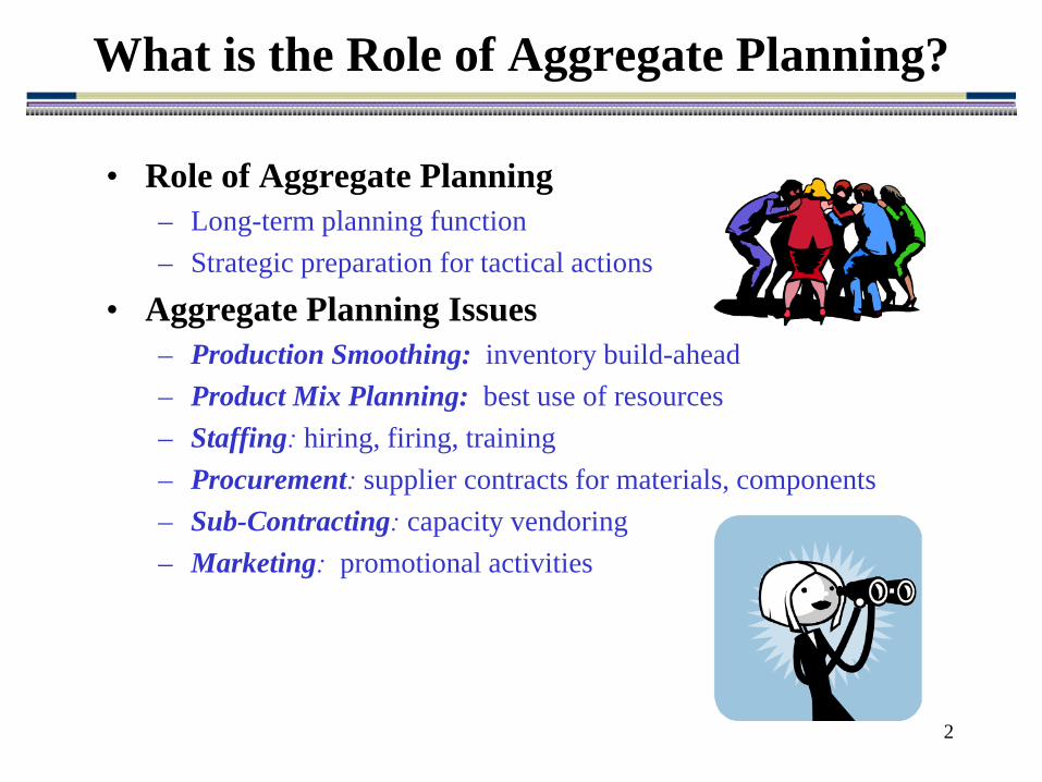
What is the Role of Aggregate Planning?

• Role of Aggregate Planning– Long-term planning function– Strategic preparation for tactical actions

• Aggregate Planning Issues– Production Smoothing: inventory build-ahead– Product Mix Planning: best use of resources– Staffing: hiring, firing, training– Procurement: supplier contracts for materials, components– Sub-Contracting: capacity vendoring– Marketing: promotional activities

3

Aggregate Planning is Long Term

PersonnelPlan

FORECASTING

CAPACITY/FACILITYPLANNING

WORKFORCE PLANNING

MarketingParameters

Product/ProcessParameters

LaborPolicies

CapacityPlan

AGGREGATEPLANNING

AggregatePlan Strategy

WorkSchedule

WIP/QUOTASETTING

DEMANDMANAGEMENT

SEQUENCING & SCHEDULING

CustomerDemands

MasterProductionSchedule

SHOP FLOORCONTROL

WIPPosition Tactics

REAL-TIMESIMULATION

PRODUCTIONTRACKING

WorkForecast

Control

4

Basic Aggregate Planning Situation

• Problem: plan production of single product over planning horizon.

• Motivation for Study:– mechanics and value of Linear Programming (LP) as a tool– intuition of production smoothing

• Inputs:– demand forecast (over planning horizon)– capacity constraints– unit profit– inventory carrying cost rate

5

A Simple Aggregate Planning Model (I)

Notation:

. period of end at theinventory . period during soldquantity

. period during producedquantity period. onefor inventory ofunit one hold cost to

cost) holding including(not profit unit . periodin capacity . periodin demand

.,.......,1 periods,timetheofindex an

tItS

tXhr

tctd

ttt

t

t

t

t

t

=======

==

6

Formulation

ttISXttSXIIttcXttdS

hIrS

ttt

tttt

tt

tt

tttt

,.....10,,,.....1,,.....1,.....1

subject to

max

1

1

=≥=−+==≤=≤

−

−

=∑

demandcapacityinventory balancenon-negativity

sales revenue - holding cost

summed over planning horizon

A Simple Aggregate Planning Model (II)

7

Product Mix Planning (I)

• Problem: determine most profitable mix over planning horizon

• Motivation for Study:– linking marketing/promotion to logistics.– Bottleneck identification.

• Inputs:– demand forecast by product (family?); may be ranges– unit hour data– capacity constraints– unit profit by product– holding cost

8

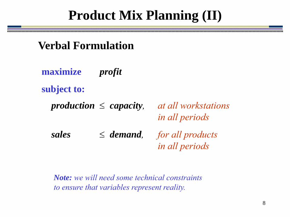
Product Mix Planning (II)

maximize profit

subject to:

production ≤ capacity, at all workstationsin all periods

sales ≤ demand, for all productsin all periods

Note: we will need some technical constraintsto ensure that variables represent reality.

Verbal Formulation

9

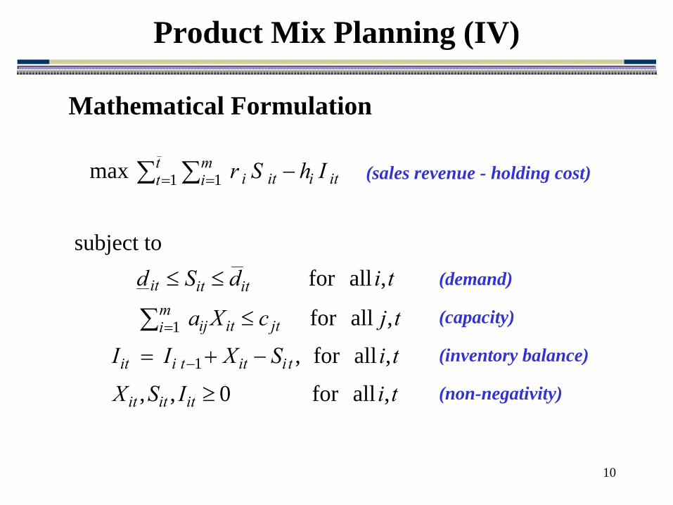
Product Mix Planning (III)

. of endat product ofinventory . periodin soldproduct ofamount

periodin produced product ofamount . period onefor ofunit one hold cost to

product ofunit one fromprofit net

. periodin on workstatiofcapacity

.product ofunit one produce totion on worksta required time periodin product of allowed sales minimum

. periodin product for demand maximum

1 period, ofindex an ,1 on, workstatiofindex an

,.....,1 product, ofindex an

tiItiS

tiXtih

ir

tjc

ijatid

tid

t,......,ttn,.....jj

mii

it

it

it

i

i

jt

ij

it

it

==

===

=

=

==

====

==

Notation

10

Product Mix Planning (IV)

tiISX

tiSXII

tjcXa

tidSd

IhSr

ititit

tiittiit

jtmi itij

ititit

itiitimi

tt

, allfor 0,,

, allfor ,

, allfor

, allfor subject to

max

1

1

11

≥

−+=

≤

≤≤

−

−

=

==

∑

∑∑

(demand)

(capacity)

(inventory balance)

(non-negativity)

(sales revenue - holding cost)

Mathematical Formulation

11

A Product Mix Example (I)

Assumptions:

Data:

• two products, P and Q• constant weekly demand, cost, capacity, etc.• Objective: maximize weekly profit

Product P Q Selling price $90 $100Raw Material Cost $45 $40Max Weekly Sales 100 50Minutes per unit on Workcenter A 15 10Minutes per unit on Workcenter B 15 35Minutes per unit on Workcenter C 15 5Minutes per unit on Workcenter D 25 14

12

A Product Mix Example (II)

Formulation:

24001425240051524003515

24001015 :subject to

50006045max

≤+≤+≤+≤+

−+

QP

QP

QP

QP

QP

XXXXXX

XX

XX

Solution:

09.36

79.75 $557.94 Objective Optimal

*

*

=

=

=

Q

P

X

X

Net Weekly Profit : Round solution down (still feasible) to:

36

75*

*

=

=

Q

P

X

X

To get $45 ×75 + $60 ×36 - $5,000 = $535.

A Linear Programming (LP) Approach:

13

Extensions to the Basic Product Mix Model (I)

Other Resource Constraints:

Utilization Matching: Let q represent fraction of rated capacity we are willing to run on resource j.

∑=

≤m

ijtitij tjqcXa

1, allfor

Notation:

Constraint for Shared Resource j: ∑=

≤m

ijtitij kXb

1

tiX

tjk

ijb

it

jt

ij

periodin produced product ofamount

periodin available resource of units ofnumber

product ofunit per required resource of units

=

=

=

14

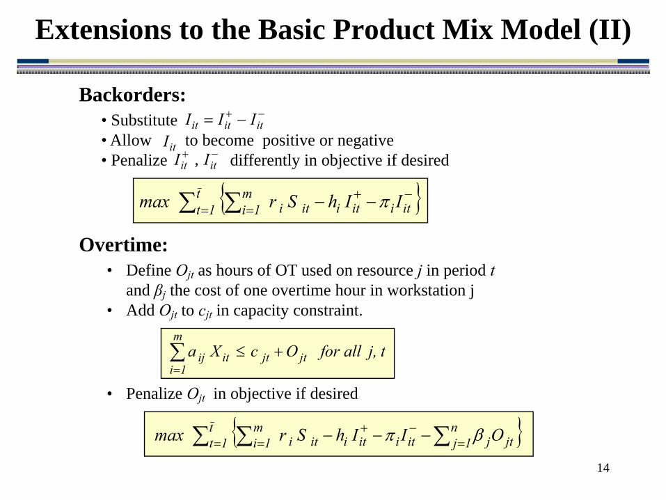
Backorders:

Overtime:

• Substitute • Allow to become positive or negative• Penalize differently in objective if desired

−+ −= ititit IIIitI

−+itit II ,

• Define Ojt as hours of OT used on resource j in period t and βj the cost of one overtime hour in workstation j

• Add Ojt to cjt in capacity constraint.

• Penalize Ojt in objective if desired

Extensions to the Basic Product Mix Model (II)

∑=

+≤m

1ijtjtitij tj, all forOcXa

{ }−+== −−∑∑ itiitiiti

m1i

t1t IIhSrmax π

{ }∑∑∑ =−+

== −−− n1j jtjitiitiiti

m1i

t1t OIIhSrmax βπ

15

Workforce Planning

• Problem: determine most profitable production and hiring/firing policy over planning horizon.

• Motivation for Study:– hiring/firing vs. overtime vs. Inventory Build tradeoff– iterative nature of optimization modeling.

• Inputs:– demand forecast (assume single product for simplicity)– unit hour data– labor content data– capacity constraints – hiring/ firing costs– overtime costs– holding costs– unit profit

16hour-man oneby workforcedecrease cost tohour-man oneby workforceincrease cost to

hour-man/dollarsin overtime ofcost hour-man / dollarsin meregular ti ofcost . period onefor unit one hold cost to

.unit one fromprofit net

. periodin center work ofcapacity unit. one produce torequired hoursman ofnumber

tion on worksta hoursunit periodin allowed sales minimum

. periodin demand maximum

1 period, ofindex an ,1 ion, workstatofindex an

=′==′===

==

=

==

====

eell

thr

tjcb

jatd

td

t,......,ttn,.....jj

jt

j

t

t

A Workforce Planning Model (I)

Notation

17

hoursin t periodin overtimeOhours.-man

in t to1 tperiod from cein workfor (fires) decreaseFhours.-man

in t to1t period from cein workfor (hires) increaseHmeregular ti of hours-manin t period workforceW

t of endat inventory It periodin soldamount S

t periodin producedamount X

t

t

t

t

t

t

t

=

−=

−=

=

=

=

=

Notation (cont.)

A Workforce Planning Model (II)

Note, this model only considers a single product. Generalizations to m products are straightforward!

18

{ }

tFHWOISXtOWbX

tFHWW

tSXII

tcXatdSd

FeeHOllWIhSr

ttttttt

ttt

tttt

tttt

jttj

ttt

ttttttt

t

allfor 0,,,,,, allfor

allfor

allfor ,

allfor allfor

subject to

max

1

1

1

≥+≤

−+=

−+=

≤≤≤

′−−′−−−

−

−

=∑

A Workforce Planning Model (III)

Formulation

19

Problem Description• 12 month planning horizon• 168 hours per month• 15 workers currently in system• regular time labor at $35 per hour• overtime labor at $52.50 per hour• $2,500 to hire and train new worker

$2,500/168=$14.88 ≈ $15/hour• $1,500 to lay off worker

$1,500/168=$8.93 ≈ $9/hour• 12 hours labor per unit• demand assumed met (St=dt, so St variables are unnecessary)

A Workforce Planning Example (I)

20

• Solution:– LP optimal Solution: layoff 9.5 workers– Add constraint: Ft=0

• results in 48 hours/worker/week of overtime– Add constraint: Ot ≤ 0.2Wt

• Reasonable solution?

A Workforce Planning Example (II)

21

Aggregate Planning Conclusions

• No single AP model is right for every situation• Simplicity promotes understanding• Linear programming is a useful AP tool• Robustness matters more than precision• Formulation and Solution are not separate activities.