AGGREGATE PLANNING AND MASTER SCHEDULINGuotechnology.edu.iq/dep-production/branch3_files/7th 8th AGGREGA… · AGGREGATE PLANNING AND MASTER SCHEDULING ... Production Planning and

AGGREGATE PLANNING AND MASTER

SCHEDULING

(Part 1)

Dr. Mahmoud Abbas Mahmoud Al-Naimi

Assistant Professor

Industrial Engineering Branch

Department of Production Engineering and Metallurgy

University of Technology

Baghdad - Iraq

[email protected]

[email protected]

2015 - 2016

mailto:[email protected]

mailto:[email protected]

6201 - 5201 Dr. Mahmoud Abbas Mahmoud Production Planning and Control

1

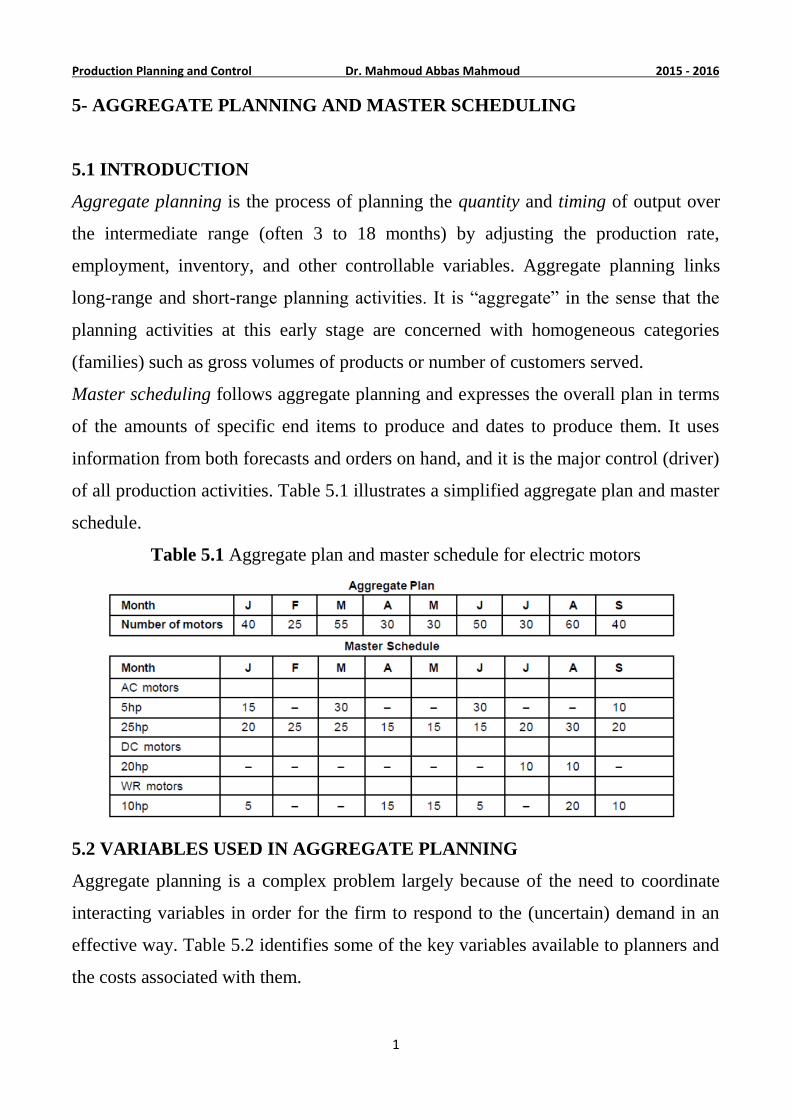
5- AGGREGATE PLANNING AND MASTER SCHEDULING

5.1 INTRODUCTION

Aggregate planning is the process of planning the quantity and timing of output over

the intermediate range (often 3 to 18 months) by adjusting the production rate,

employment, inventory, and other controllable variables. Aggregate planning links

long-range and short-range planning activities. It is “aggregate” in the sense that the

planning activities at this early stage are concerned with homogeneous categories

(families) such as gross volumes of products or number of customers served.

Master scheduling follows aggregate planning and expresses the overall plan in terms

of the amounts of specific end items to produce and dates to produce them. It uses

information from both forecasts and orders on hand, and it is the major control (driver)

of all production activities. Table 5.1 illustrates a simplified aggregate plan and master

schedule.

Table 5.1 Aggregate plan and master schedule for electric motors

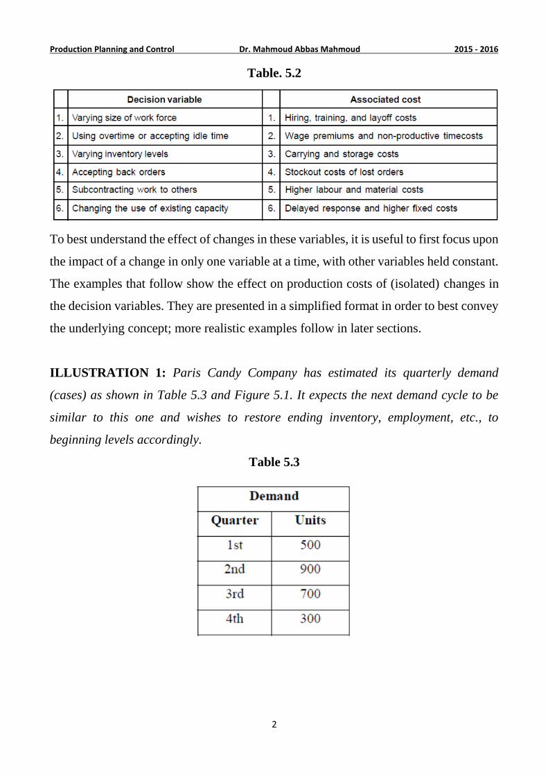
5.2 VARIABLES USED IN AGGREGATE PLANNING

Aggregate planning is a complex problem largely because of the need to coordinate

interacting variables in order for the firm to respond to the (uncertain) demand in an

effective way. Table 5.2 identifies some of the key variables available to planners and

the costs associated with them.


2

Table. 5.2

To best understand the effect of changes in these variables, it is useful to first focus upon

the impact of a change in only one variable at a time, with other variables held constant.

The examples that follow show the effect on production costs of (isolated) changes in

the decision variables. They are presented in a simplified format in order to best convey

the underlying concept; more realistic examples follow in later sections.

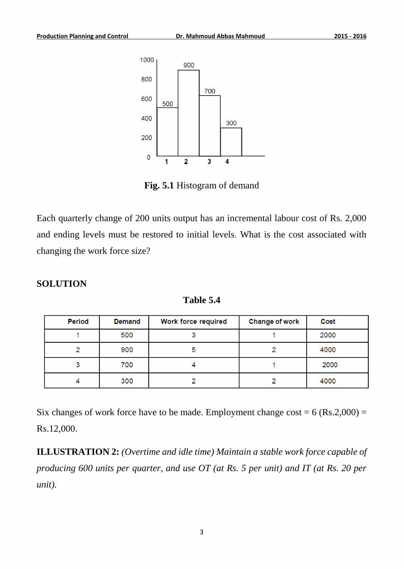
ILLUSTRATION 1: Paris Candy Company has estimated its quarterly demand

(cases) as shown in Table 5.3 and Figure 5.1. It expects the next demand cycle to be

similar to this one and wishes to restore ending inventory, employment, etc., to

beginning levels accordingly.

Table 5.3


3

Fig. 5.1 Histogram of demand

Each quarterly change of 200 units output has an incremental labour cost of Rs. 2,000

and ending levels must be restored to initial levels. What is the cost associated with

changing the work force size?

SOLUTION

Table 5.4

Six changes of work force have to be made. Employment change cost = 6 (Rs.2,000) =

Rs.12,000.

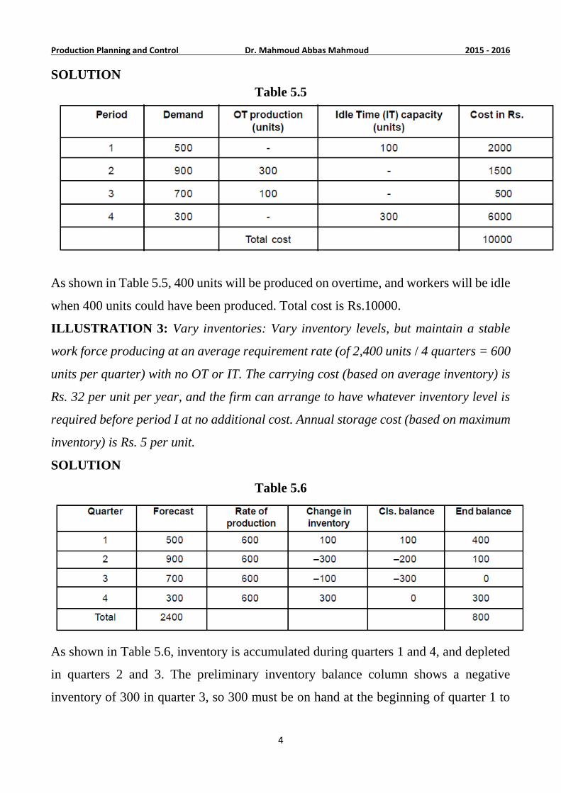
ILLUSTRATION 2: (Overtime and idle time) Maintain a stable work force capable of

producing 600 units per quarter, and use OT (at Rs. 5 per unit) and IT (at Rs. 20 per

unit).


4

SOLUTION

Table 5.5

As shown in Table 5.5, 400 units will be produced on overtime, and workers will be idle

when 400 units could have been produced. Total cost is Rs.10000.

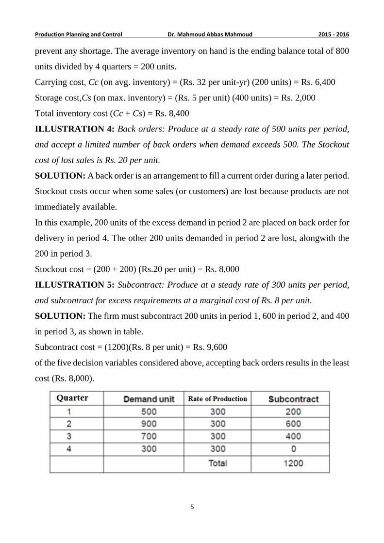
ILLUSTRATION 3: Vary inventories: Vary inventory levels, but maintain a stable

work force producing at an average requirement rate (of 2,400 units / 4 quarters = 600

units per quarter) with no OT or IT. The carrying cost (based on average inventory) is

Rs. 32 per unit per year, and the firm can arrange to have whatever inventory level is

required before period I at no additional cost. Annual storage cost (based on maximum

inventory) is Rs. 5 per unit.

SOLUTION

Table 5.6

As shown in Table 5.6, inventory is accumulated during quarters 1 and 4, and depleted

in quarters 2 and 3. The preliminary inventory balance column shows a negative

inventory of 300 in quarter 3, so 300 must be on hand at the beginning of quarter 1 to


5

prevent any shortage. The average inventory on hand is the ending balance total of 800

units divided by 4 quarters = 200 units.

Carrying cost, Cc (on avg. inventory) = (Rs. 32 per unit-yr) (200 units) = Rs. 6,400

Storage cost,Cs (on max. inventory) = (Rs. 5 per unit) (400 units) = Rs. 2,000

Total inventory cost (Cc + Cs) = Rs. 8,400

ILLUSTRATION 4: Back orders: Produce at a steady rate of 500 units per period,

and accept a limited number of back orders when demand exceeds 500. The Stockout

cost of lost sales is Rs. 20 per unit.

SOLUTION: A back order is an arrangement to fill a current order during a later period.

Stockout costs occur when some sales (or customers) are lost because products are not

immediately available.

In this example, 200 units of the excess demand in period 2 are placed on back order for

delivery in period 4. The other 200 units demanded in period 2 are lost, alongwith the

200 in period 3.

Stockout cost = (200 + 200) (Rs.20 per unit) = Rs. 8,000

ILLUSTRATION 5: Subcontract: Produce at a steady rate of 300 units per period,

and subcontract for excess requirements at a marginal cost of Rs. 8 per unit.

SOLUTION: The firm must subcontract 200 units in period 1, 600 in period 2, and 400

in period 3, as shown in table.

Subcontract cost = (1200)(Rs. 8 per unit) = Rs. 9,600

of the five decision variables considered above, accepting back orders results in the least

cost (Rs. 8,000).


6

5.3 AGGREGATE PLANNING STRATEGIES

Several different strategies have been employed to assist in aggregate planning. Three

“pure”strategies are recognized. The pure strategies stem from early models that

depicted production results when only one of the decision variables was permitted to

vary all others being held constant. Three focused strategies are:

1. Vary production to match demand by changes in employment (Chase demand

strategy): This strategy permits hiring and layoff of workers, use of overtime, and

subcontracting as required in each period. However, inventory build-up is not used.

2. Produce at a constant rate and use inventories. (Level production strategy): This

strategy retains a stable work force producing at a constant output rate. Inventory can

be accumulated to satisfy peak demands. In addition, subcontracting is allowed and back

orders can be accepted.Promotional programs may also be used to shift demand.

3. Produce with stable workforce but vary the utilization rate (Stable work-force

strategy): This strategy retains a stable work force but permits overtime, part-time, and

idle time. Some versions of this strategy permit back orders, subcontracting, and use of

inventories. Although this strategy uses overtime, it avoids the detrimental effects of

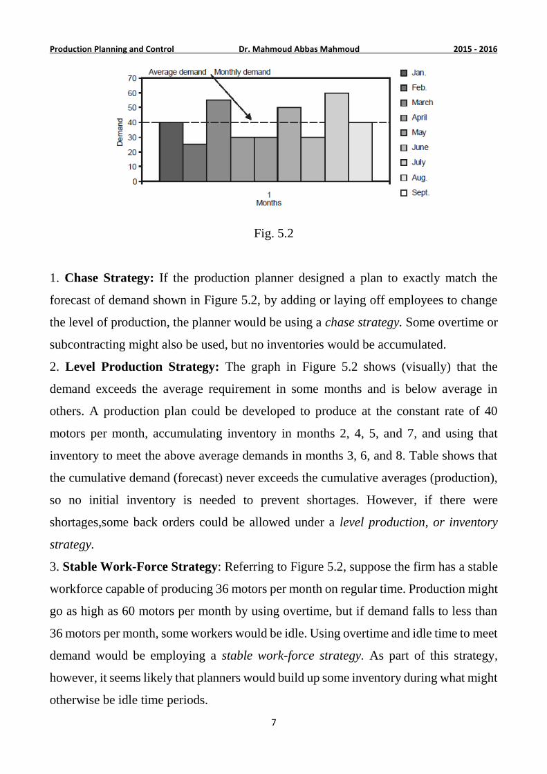
layoff. We can use the following data in Figs. 5.2 and 5.3 to illustrate the three focused

strategies described above. These figures display a histogram of a 9-month forecast for

motors. The total requirement for the 9 months is 360 motors. This works out to an

average (mean) of 40 motors per month, which is shown as a dotted line in Figure 5.2.

Table 5.7


7

Fig. 5.2

1. Chase Strategy: If the production planner designed a plan to exactly match the

forecast of demand shown in Figure 5.2, by adding or laying off employees to change

the level of production, the planner would be using a chase strategy. Some overtime or

subcontracting might also be used, but no inventories would be accumulated.

2. Level Production Strategy: The graph in Figure 5.2 shows (visually) that the

demand exceeds the average requirement in some months and is below average in

others. A production plan could be developed to produce at the constant rate of 40

motors per month, accumulating inventory in months 2, 4, 5, and 7, and using that

inventory to meet the above average demands in months 3, 6, and 8. Table shows that

the cumulative demand (forecast) never exceeds the cumulative averages (production),

so no initial inventory is needed to prevent shortages. However, if there were

shortages,some back orders could be allowed under a level production, or inventory

strategy.

3. Stable Work-Force Strategy: Referring to Figure 5.2, suppose the firm has a stable

workforce capable of producing 36 motors per month on regular time. Production might

go as high as 60 motors per month by using overtime, but if demand falls to less than

36 motors per month, some workers would be idle. Using overtime and idle time to meet

demand would be employing a stable work-force strategy. As part of this strategy,

however, it seems likely that planners would build up some inventory during what might

otherwise be idle time periods.


8

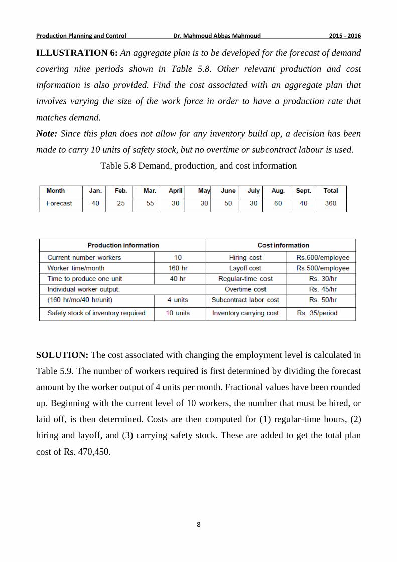
ILLUSTRATION 6: An aggregate plan is to be developed for the forecast of demand

covering nine periods shown in Table 5.8. Other relevant production and cost

information is also provided. Find the cost associated with an aggregate plan that

involves varying the size of the work force in order to have a production rate that

matches demand.

Note: Since this plan does not allow for any inventory build up, a decision has been

made to carry 10 units of safety stock, but no overtime or subcontract labour is used.

Table 5.8 Demand, production, and cost information

SOLUTION: The cost associated with changing the employment level is calculated in

Table 5.9. The number of workers required is first determined by dividing the forecast

amount by the worker output of 4 units per month. Fractional values have been rounded

up. Beginning with the current level of 10 workers, the number that must be hired, or

laid off, is then determined. Costs are then computed for (1) regular-time hours, (2)

hiring and layoff, and (3) carrying safety stock. These are added to get the total plan

cost of Rs. 470,450.


9

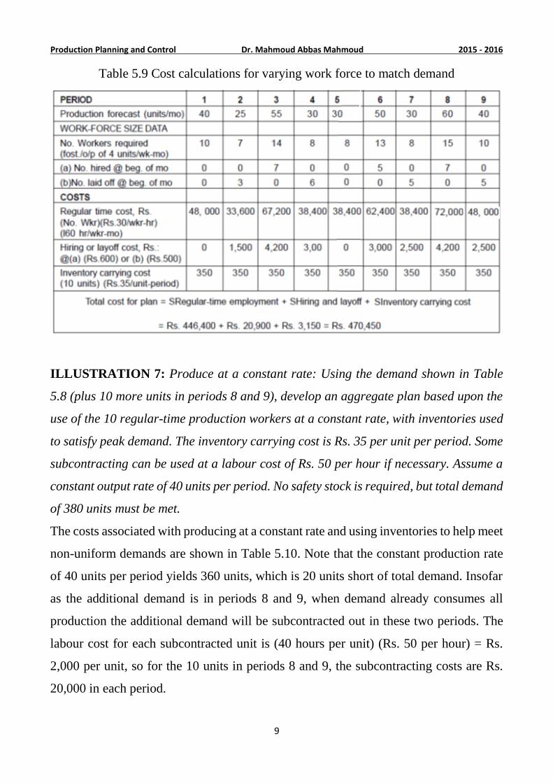
Table 5.9 Cost calculations for varying work force to match demand

ILLUSTRATION 7: Produce at a constant rate: Using the demand shown in Table

5.8 (plus 10 more units in periods 8 and 9), develop an aggregate plan based upon the

use of the 10 regular-time production workers at a constant rate, with inventories used

to satisfy peak demand. The inventory carrying cost is Rs. 35 per unit per period. Some

subcontracting can be used at a labour cost of Rs. 50 per hour if necessary. Assume a

constant output rate of 40 units per period. No safety stock is required, but total demand

of 380 units must be met.

The costs associated with producing at a constant rate and using inventories to help meet

non-uniform demands are shown in Table 5.10. Note that the constant production rate

of 40 units per period yields 360 units, which is 20 units short of total demand. Insofar

as the additional demand is in periods 8 and 9, when demand already consumes all

production the additional demand will be subcontracted out in these two periods. The

labour cost for each subcontracted unit is (40 hours per unit) (Rs. 50 per hour) = Rs.

2,000 per unit, so for the 10 units in periods 8 and 9, the subcontracting costs are Rs.

20,000 in each period.


10

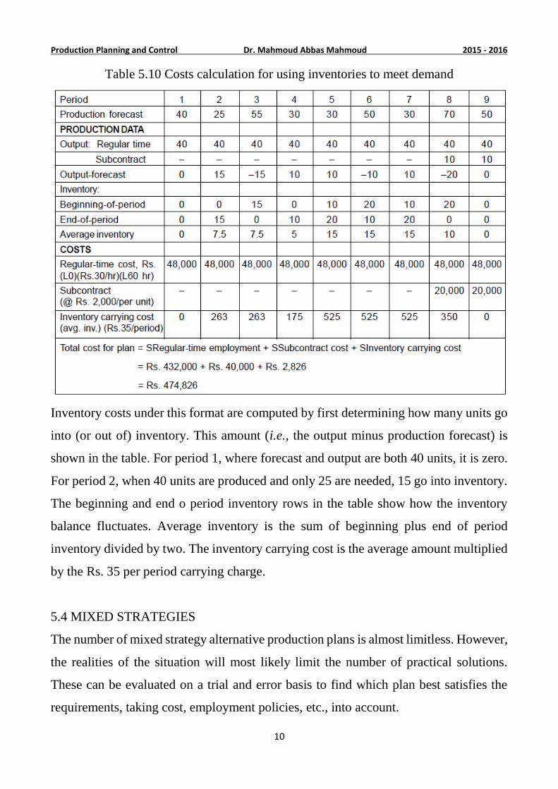
Table 5.10 Costs calculation for using inventories to meet demand

Inventory costs under this format are computed by first determining how many units go

into (or out of) inventory. This amount (i.e., the output minus production forecast) is

shown in the table. For period 1, where forecast and output are both 40 units, it is zero.

For period 2, when 40 units are produced and only 25 are needed, 15 go into inventory.

The beginning and end o period inventory rows in the table show how the inventory

balance fluctuates. Average inventory is the sum of beginning plus end of period

inventory divided by two. The inventory carrying cost is the average amount multiplied

by the Rs. 35 per period carrying charge.

5.4 MIXED STRATEGIES

The number of mixed strategy alternative production plans is almost limitless. However,

the realities of the situation will most likely limit the number of practical solutions.

These can be evaluated on a trial and error basis to find which plan best satisfies the

requirements, taking cost, employment policies, etc., into account.


11

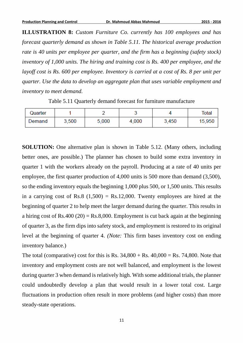
ILLUSTRATION 8: Custom Furniture Co. currently has 100 employees and has

forecast quarterly demand as shown in Table 5.11. The historical average production

rate is 40 units per employee per quarter, and the firm has a beginning (safety stock)

inventory of 1,000 units. The hiring and training cost is Rs. 400 per employee, and the

layoff cost is Rs. 600 per employee. Inventory is carried at a cost of Rs. 8 per unit per

quarter. Use the data to develop an aggregate plan that uses variable employment and

inventory to meet demand.

Table 5.11 Quarterly demand forecast for furniture manufacture

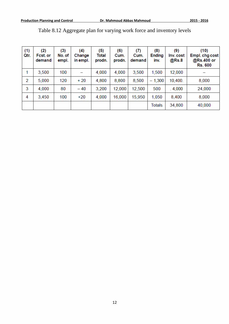
SOLUTION: One alternative plan is shown in Table 5.12. (Many others, including

better ones, are possible.) The planner has chosen to build some extra inventory in

quarter 1 with the workers already on the payroll. Producing at a rate of 40 units per

employee, the first quarter production of 4,000 units is 500 more than demand (3,500),

so the ending inventory equals the beginning 1,000 plus 500, or 1,500 units. This results

in a carrying cost of Rs.8 (1,500) = Rs.12,000. Twenty employees are hired at the

beginning of quarter 2 to help meet the larger demand during the quarter. This results in

a hiring cost of Rs.400 (20) = Rs.8,000. Employment is cut back again at the beginning

of quarter 3, as the firm dips into safety stock, and employment is restored to its original

level at the beginning of quarter 4. (Note: This firm bases inventory cost on ending

inventory balance.)

The total (comparative) cost for this is Rs. 34,800 + Rs. 40,000 = Rs. 74,800. Note that

inventory and employment costs are not well balanced, and employment is the lowest

during quarter 3 when demand is relatively high. With some additional trials, the planner

could undoubtedly develop a plan that would result in a lower total cost. Large

fluctuations in production often result in more problems (and higher costs) than more

steady-state operations.


12

Table 8.12 Aggregate plan for varying work force and inventory levels

Documents

AGGREGATE PLANNING AND MASTER SCHEDULINGuotechnology.edu.iq/dep-production/branch3_files/7th 8th AGGREGA… · AGGREGATE PLANNING AND MASTER SCHEDULING ... Production Planning and