Embed Size (px)
Citation preview

Agile Project Dynamics:
A System Dynamics Investigation of
Agile Software Development Methods
Firas Glaiel
Allen Moulton
Stuart Madnick
Working Paper CISL# 2013-05
March 2013
Composite Information Systems Laboratory (CISL)
Sloan School of Management, Room E62-422
Massachusetts Institute of Technology
Cambridge, MA 02142

1
Agile Project Dynamics: A System Dynamics Investigation of
Agile Software Development Methods
Firas S. Glaiel Raytheon Company and
MIT Sloan School of Management
firasg @mit.edu
Allen Moulton MIT Sloan School of Management
and Engineering Systems Division
amoulton @mit.edu
Stuart E. Madnick MIT Sloan School of Management
and Engineering Systems Division
smadnick @mit.edu
Abstract— While Agile software development has many advocates, acceptance in the
government and defense sectors has been limited. To address questions of meanings to the term
“Agile,” we examine a range of Agile methods practiced and develop a framework of seven
characteristics, which we call the Agile Genome. We gain insight into the dynamics of how
Agile development compares to classic “waterfall” approaches by constructing a System
Dynamics model for software projects. The Agile Project Dynamics (APD) model captures each
of the Agile genes as a separate component of the model and allows experimentation with
combinations of practices and management policies. Experimentation with the APD model is
used to explore how different genes work in combination with one another to produce both
positive and negative effects. The extensible design of the APD model provides the basis for
further study of Agile methods and management practices.
1. Introduction
In the commercial sector, many organizations have embraced Agile methodologies as the way
to better flexibility, greater responsiveness, and improved time-to-market in the development of
software. Forrester Research surveys of 1000+ IT professionals in 2009 and in 2010, showed a
decline in the use of “Traditional” development methodologies, and a rise in adoption of Agile.
About 40% of organizations reported using one or another of the Agile family of methodologies
[29,30]. Studies show a wide range of positive effects of Agile: 5% to 61% reductions in cost,
24% to 58% reductions in development time, and 11% to 83% reductions in product defects [33].
Despite these results, in the government, and particularly the defense sector, Agile is resisted.
A 2010 study of Agile in defense software acquisition [32] found that Agile was only likely to be
used in two circumstances: 1) the program is urgent and mission critical for combat forces and has
the clout to get a waiver from the normal process, or 2) the program is failing and likely to be
canceled.
This research uses System Dynamics to examine the characteristics of so-called “Agile”
software development methodologies. We focus specifically on large-scale government-type
software development efforts – though many of the findings apply to the private sector as well.
Our objective is to use System Dynamics to help answer these questions:
What do people really mean by “Agile”?
Why the wide variation in reported ROI compared to traditional methods?
Can Agile ever make things worse?
What are management options and implications? and
Can Agile succeed in the large-scale government systems development domain?
1.1 Agile and Speed of Requirements Change
A common attitude in the software industry has been that Agile only works for small-scale
projects with small experienced teams, and that traditional Waterfall is better suited for larger
scale projects. Large-scale software engineering organizations have traditionally used plan-driven,

2
heavyweight, waterfall-style approaches for the planning, execution, and monitoring of software
development efforts. This approach often results in relatively long development schedules that are
susceptible to failure, especially in a rapidly changing environment. Schedule pressure, defects,
and requirements changes can drive endless redesign, delay the project, and incur extra cost. The
success of the waterfall development life cycle is dependent upon a stable business environment
(i.e. stable requirements) and breaks down in a high change environment [16]. Whether it is to
support the war efforts in the 2000s, to address rapidly-evolving cyber-security threats, or to
compete in an ever-more net-centric world: the demands of the government software customer
today are such that capabilities are needed on shorter time horizons, quality is expected out of the
gate. Software producers are expected to be nimble enough to mirror the fast-paced changes in
their customer’s needs and environment changes [33].
Taking inspiration from the world of biology, Charles Fine argues that each industry has its
own evolutionary life cycle (or “clockspeed”), measured by the rate at which it introduces new
products, processes, and organizational structures[13]. The government systems software market
had historically been a slow-to-medium-clockspeed environment, with software being only a
component within large multi-year programs. It is now becoming a fast-clockspeed environment,
with demand for quick software delivery to run on existing networks, infrastructure, and systems.
Fine argues that firms must adapt to the changing environment to maintain any competitive
advantage. Government software contractors must then adapt to survive. The government
software contractor community is looking at Agile development to deliver capabilities at the pace
and cost needed to stay competitive in the new government software market.
Many in the consumer-faced commercial software sector have dealt with a fast-clockspeed
environment by adopting Agile software development, since it was designed to be flexible and
responsive to high rates of change. The promise of Agile is that it will help organizations lower
costs and shorten development times while improving quality.
1.2 Agile in Government Software Development
Previous results [28] have found dramatic differences in the performance of commercial
software development compared to defense. Defense takes much longer and goes through more
cycles to refine defects out of software products. Commercial and defense sectors differ in the
control system that determines the value of the product. Government and defense (as well as some
bureaucratic parts of private organizations) do not have a market to set value. Defense also
operates by contracting out software development and has evolved elaborate bureaucratic
planning processes that try to control costs, expedite delivery, and make sure the government gets
value for its money. These processes were originally developed to control large weapons systems
acquisitions programs (for aircraft, tanks, ships, etc.) and transferred to software acquisition
(including software development)[15].
Concerns about the sluggishness of large scale government and defense IT development has
been expressed repeatedly for over thirty years. A 2009 Defense Science Board report found that
the average time from concept to initial operating capability was 91 months – over seven years
[17]. As long ago as 1982, a defense study recommended an agile-like process to “buy a little, test
a little” to minimize overall software development exposure and risk [14]. Thirty years later, a
2012 Brookings study found a “growing consensus on the need for agile approaches” in defense
IT system acquisition[15].
In 2010, then Under Secretary of Defense for Acquisition, Technology and Logistics, Dr.
Ashton Carter issued a memo entitled “Better Buying Power: Guidance for Obtaining Greater
Efficiency and Productivity in Defense Spending.” He was on a mission to rein in cost overruns

3
and spending as part of an overall plan to cut $100 billion from the Pentagon budget over the
subsequent five years. Carter also directed acquisition managers to award more services contracts
to small businesses to increase competition and provide with “an important degree of agility and
innovation,” with lower overhead costs[4].
The big government software contractors took note… The Pentagon budget is shrinking and
they now will increasingly have to compete with small/nimble firms for contracts. This is perhaps
the single driving force behind why these companies are taking a serious look at disrupting their
mature product development practices by incorporating Agile software development as practiced
in the commercial world, including in today’s dominant “born-on-the-web” software giants like
Google, Facebook, and Amazon.
1.3 Plan of the Paper
Software development teams that are said to employ “Agile development” make use of a
variety of practices that are advertised to reduce coordination costs, to focus teams on capability
objectives, and to produce stable product iterations that can be released incrementally. Agile
software development has become a de-facto approach to the engineering of software systems in
the web-based and other consumer-faced software sector and is now entering aerospace and
defense. But it is not clear whether Agile can work in these risk-averse and heavily plan-based
environments.
In section 2, we present a framework for understanding Agile systems development practices,
which we call the “Agile Genome.” A study of a broad range of Agile methodologies leads us to
the identification of seven representative characteristics of Agile software projects: 1)
story/feature-driven, 2) iterative-incremental, 3) micro-optimizing, 4) refactoring, 5) continuous
integration, 6) team dynamics, and 7) customer involvement.
In section 3, we describe the System Dynamics model developed in this research, which we
call the Agile Project Dynamics (APD) model. In developing an Agile software development
project model, the Agile Genome provided structure for capturing of the impact of each of the
Agile genes on the emergent behavior of medium to large scale software development projects.
System Dynamics models can be used to aid in proactive, strategic/tactical management of design
and development projects [11]. Our modeling of Agile projects builds upon an existing model and
integrative view of software development project management [12] that models the classic
Waterfall approach to development.
In section 4, we illustrate the use of the model in experiments to study how agile methods can
be successfully applied within the context of government and defense software acquisition. The
model helps to understand and simulate the impact of alternative management policies involving
the adoption of one, many, or all of the Agile genes and to compare resulting project performance
in terms of cost, schedule, and quality. The model can be used to compare the performance of
projects using classic Waterfall-style approaches versus those using various Agile methodologies
and combinations of Agile practices.
Section 5 presents conclusions and directions for future research.
2. Identifying The Agile Genome
As part of an effort to develop a System Dynamics model, which can be used to understand the
impact of Agile practices on software and systems engineering project performance, there was a
need to identify and characterize “agile” practices employed by software and system development
organizations. In other words: in order to model the dynamic effects of agile practices, we had to
first understand the “essence of agility”: What makes development Agile?

4
We reviewed a range of common Agile development methodologies, including Scrum[6],
eXtreme Programming, Feature Driven Design, and Test Driven Design. After review and
analysis of many approaches, we found that they share common characteristics. The project teams
that employ these methodologies in effect practice combinations of some or all of seven
remarkably similar “agile techniques.” We call these “the Genome of Agile,” consisting of the
seven genes shown in Table 1. Each of these genes will be described in the following sections.
Table 2 showing how the genes map to some popular methodologies is included in section 2.8 .
Gene Name Short Description
Story/Feature Driven Break up of project into manageable pieces of functionality; sometimes named “features”, “stories”, “use cases”, or “threads”.
Iterative-Incremental Development is performed in repeated cycles (iterative) and in portions at a time (incremental.)
Micro-Optimizing Teams are empowered to modify aspects of the process or dynamically adapt to changing circumstances. Small improvements and variable changes are made frequently and as needed.
Refactoring Refinement of the software design and architecture to improve software maintainability and flexibility.
Continuous Integration Policies and practices related to Configuration Management, and software build and test automation.
Team Dynamics “Soft” factors related to the project team. Daily meetings, agile workspaces, pair programming, schedule/peer pressure, experience gain, etc.
Customer-Involvement Customer/User involved in demonstrations of functionality to verify/validate features. Higher frequency feedback and clarification of uncertainty. Availability to participate in development meetings.
Table 1 - The Genome of Agile
2.1 Story/Feature Driven
Most Agile projects decompose the system being developed into manageable sets of
“features” or “stories.” The terminology differs (“use case”, “thread”, “feature”, “capability,”
etc) across methodologies and organizations, but the concept is the same: The system is
segmented into sets of client-valued functionality, and development work is organized around
producing these features. An advantage of the feature driven paradigm is that, as features are
produced, they become available for early deployment, customer demonstrations, or early
integration and test activities – all of which can help reduce uncertainty, detect functional defects
early in the development cycle, or deliver early capabilities to customers (as opposed to waiting
for a full-featured product). Decomposing a system into feature sets allows functional problems
and requirements issues to be identified much earlier (as soon as each feature is implemented and
available to be tested).
In contrast, traditional approaches generally employ “Functional Decomposition” where a
system is broken into sub-components (e.g. user-interface component, database component, etc)
which are implemented in parallel, and integrated in late stages of development.[1] For this
“waterfall” approach to be viable, the up-front requirements specifications must be locked-down
and perfectly match the ultimate needs of users. Despite requirements lock-down, functional and
requirements issues can surface late in the project, when the integrated system becomes visible in
functionally testing.
From a management perspective, the feature driven approach also yields a concrete measure
of progress by feature (i.e. 9 out of 10 features implemented means 90% complete, assuming all

5
features weighted equally.) This differs from traditional measures of progress, based on arguably
arbitrary milestones, where for example, the completion of a design phase might translate to
claiming forty percent of the project complete. One class of problems associated with using a
functional decomposition approach is that a project can report to be at 90% completion, yet still
have no functioning software to show for it.
2.2 Iterative-Incremental
Whereas traditional development approaches call for complete requirements analysis phase,
followed by lengthy design, coding, and test phases, Agile projects tend to develop an initial
increment of software which then incrementally evolves into the final product through a series of
short design/code/test iterations. This allows development to begin without necessarily having
completely finalized requirements.
This gene combines with the Feature-Driven gene to allow the system to continually evolve
as a series of increments, each one adding more features to the existing previous incarnation. The
Iterative-Incremental concept is neither novel nor unique to Agile methodologies. In fact,
extensive use of Incremental Iterative Development (IID) for major software development efforts
dates back to the Sixties[3].
Figure 1 illustrates the process of Feature-Driven and Iterative-Incremental development. On
the far left is the Product Backlog, which consists of the required features to be built. On the far
right is the Delivered Product which is shipped to the customer. In the middle are successively
smaller cycles – releases and sprints. The pitcher on top of the Product Backlog is a reminder
that requirements often change over time.
In a single-pass waterfall development project, there would be no middle stages. The entire
product requirements set would be put through a plan-driven process aimed at delivering the
product in one step. Incremental Iterative Development uses many of the same plan-driven
processes, but delivers software in a series of releases, each adding new functionality, often
spaced at 6-12 month intervals. The best value is obtained when iterations are designed such that
early tasks help resolve uncertainty later in the project. Rather than one big design phase, one big
implementation phase, one big integration phase, then one big test phase, many iterations are
performed, each consisting of a shorter design-implement-integrate-test cycle. In Figure 1,
required features from the Product Backlog are selected and transferred to the Release Backlog.
Figure 1 Feature-Driven and Iterative-Incremental Development

6
After development is completed, a Shippable Release is produced, which then becomes part of
the Delivered Product.
One principle of the Agile Manifesto[2] is to “deliver working software frequently, from a
couple of weeks to a couple of months.” Development is performed in repeated cycles (iterative)
and in segments of work at a time (incremental.) This allows developers to focus on short-term
objectives while taking advantage of what was learned during earlier development in later
iterations. Figure 1 illustrates the frequent cycles of the Agile approach as a series of time-boxed
“sprints,” each of which moves a subset of the Release Backlog into a Sprint Backlog and
produces a Potentially Shippable Product Increment in a fixed period of time (often 2-4 weeks).
The diagram also shows a Daily Scrum meeting that is used in some forms of Agile to help keep
the project team on target. The product of all the sprints accumulates into a release, which in turn
becomes the deliverable product.
2.3 Micro-Optimizing
The Micro-Optimizing gene represents the adaptive nature of Agile management processes.
We employ the term “Optimizing” because Agile teams in most Agile methodologies are
encouraged to tailor aspects of the development process to dynamically adapt to changing
circumstances. “Micro” indicates small process adjustments and improvements made frequently.
Micro-optimizing also includes a Double Loop Learning [5] effect where the team steps back,
reviews results, questions assumptions and goals, and revises them to improve future results.
This contrasts with Single Loop Learning where an individual or a team learns to be more
efficient and productive from repetition of similar tasks. In other words, double loop learning
changes “what we do” rather than “how we do it”.
Classic development processes can exhibit a “light” flavor of this gene in the form of “Lessons
Learned” activities that are called for at the completion of a project, but which rarely feeds into
the next development cycle and yields little improvement effect on subsequent development
projects. In the context of Agile, however, iterations (e.g. sprints) are short and frequent enough
so that process adjustment is near-continuous throughout the life of a project in between
iterations. For example, the Crystal family of methods calls for “reflection workshops” to be held
every few weeks.
Teams are also trusted to self-adjust and gradually learn about how much work they can handle
in a given period of time. For example, the measure of “Sprint Velocity” in Scrum represents
how much product backlog a team can handle in one sprint. It is established as the team learns
about the project and about working with each other. Typically, team velocity improves as sprint
cycles are completed and experience gained.
2.4 Refactoring
Several agile methodologies consider refactoring to be a primary development practice.
Refactoring consists of taking apart existing working code, factoring out common elements, and
rebuilding it to provide a stronger base for subsequent development. It can also mean refining the
design or architecture of the system to allow for greater flexibility and extensibility.
Refactoring has the disadvantage that it takes extra effort and requires changing baseline
software without any direct or apparent return on investment (ROI). A project manager may ask
“why are we spending effort re-designing portions of the system unrelated to the next planned set
of features?” The answer is that future development will be lower cost and higher quality if the
code base is restructured now.

7
The downside of a feature-driven and iterative-incremental approach is that over time, the
product/system starts to exhibit signs of having “high coupling” and “low cohesion,” making it
harder (and more costly) to maintain and evolve. Coupling refers to the degree to which system
components depend on each other – in a system with high coupling there is a high degree of
dependency; changes to one element is likely to have ripple effects and impact on the behavior of
other elements. Cohesion is a measure of how strongly related the responsibilities of a single
component are – low cohesion is an indicator of lack of structure in the system. Over time, the
evolution of a system feature-by-feature, incrementally, can lead to “high coupling” and “low
cohesion,” making new changes increasingly more difficult.
One metaphor for this effect is “technical/design debt.” Similar to credit debt, technical debt
accrues interest payments in the form of extra effort that must be made in subsequent
development cycles. The practice of refactoring pays off “technical/design debt” which has
accrued over time, especially when incremental and evolutionary design results in a sub-optimal
or inflexible architecture, duplication, and other undesirable side effects.
2.5 Continuous Integration
Continuous Integration involves methods of maintaining an updated code base that includes
all changes that have been made and regularly building a testable version of the product. Agile
projects often include policies and approaches to Configuration Management (CM) as well as
automation of development workflow and processes. Automation can speed up development by
eliminating repetitive and manual tasks.
Configuration Management– Traditionally, the popular CM approach is to have different
teams develop portions of software in isolated environments (i.e. separate “branches” of a version
tree), and integrate their work products later in the development cycle. However, we know that
the later in development that a defect is found, the costlier it is to fix.[8] Moreover, significant
number of defects are interface defects.[9] Thus it can be very advantageous to integrate
components early and often.
In the mid-1990s, Microsoft moved to a "synch-and-stabilize" process which relied on daily
builds for frequent synchronizations and incremental milestones for periodic stabilizations of the
products under development.[10] This is one of the early examples of frequently integrating
various pieces of software under development to detect early conflicts.
Automated Testing – Continuous Integration includes test automation at various levels, from
unit testing of individual software modules, up to system-level functional tests. Test automation
complements the automation of other manual tasks, such as software builds.
There can be a significant up-front cost associated with developing test suites and an
infrastructure to support them. Nevertheless, there are benefits from having software perform
testing that would otherwise need to be done manually. Once tests have been automated, they can
be run quickly and repeatedly. Systems that have a long maintenance life can benefit from an
automated regression test suite – legacy projects for these types of systems often require copious
and costly manual regression testing to verify that there is no breakage in baseline functionality
introduced by added features. When Agile software is developed incrementally, automated testing
assures that new development integrates with prior work.
2.6 Team Dynamics
The Team Dynamics gene represents the collection of “soft factors” and effects related to
unique practices that influence the development team’s performance. The majority of Agile
methods call for frequent meetings to allow teams to self-organize, prioritize, and assign tasks,

8
while communicating roadblocks. The most efficient and effective method of conveying
information to and within a development team is face-to-face conversation.[7] Practices such as
“pair programming,” and attitudes such as “collective code ownership” are also claimed to have
positive effects on project performance. Team co-location and open workspaces and environments
are also preferred. These help promote the flow of information between and drive team
performance through transparency.
Another unique team dynamic that emerges in agile teams is a distinctive “social/schedule
pressure” effect. In Scrum, for example, as teams convene daily to report on what they are doing,
what they have done, and what they plan to do next, a certain level of peer pressure comes into
play, driving individuals to perform at a higher productivity. When paired with short
increments/sprints, this produces more frequent bouts of schedule pressure coinciding with the
end of each time-boxed iteration, as opposed to a single schedule crunch at the end of a waterfall
project.
2.7 Customer-Involvement
The Customer Involvement gene means accepting changing requirements and including the
user and/or customer in the development team (to the degree that this is possible). This can be in
daily stand-up meetings, design reviews and product demos. The customer’s availability and input
to the development process helps to reduce uncertainty and identify rework early. This requires
collaborating with the user/customer to evolve the requirements throughout the process – with
later requirements informed by insights gained from earlier development.
This gene can exhibit itself even on projects which appear prima facie to be “non-agile.”
Large classic Waterfall projects may hold User Involvement Events (UIEs) or deliver proof-of-
concept prototypes. These types of activities can help to clarify requirements and improve
responsiveness to customers early in the design/architecture phases.
A more traditional contracting approach is to lock-in the system requirements early on in the
project. Any subsequent change requires contractual re-negotiations for “added scope” or “scope
change”. This type of project control mechanism is intended to help keep the size of the project
in check (thus helping limit growth in costs and schedule). Nevertheless, it may mean that a long
time is spent up-front developing, refining, and validating requirements. By the time the product
is delivered, it may well meet the specifications agreed to contractually, but not be what is really
need to support the mission, especially in light of changing mission needs. Many requirements
agreed to up front turn out to be unnecessary, while other capabilities were not known and not
delivered.
There are two distinct problems with a “fixed requirements” attitude: (1) The “ah-hah”
moment: the first time that you actually use the working product. You immediately think of 20
ways you could have made it better. Unfortunately, these very valuable insights often come at the
end.[6] When requirements are locked-in up front, there is no room for making the product
better later in the development cycle. (2) Undetected requirements defects can wreak havoc on a
project if detected late in the schedule. Indeed, that is one of the reasons that the Waterfall
method came to be, to lock-down and specify the requirements so that later development could
proceed without turbulence. However, as discussed previously, when real user needs are
changing, requirements must evolve.
Often the customer interfaces with the contractor’s business operations and project managers.
Requirements are generated by business analysts (in some industries “system engineers” or
“domain experts”) and are flowed down to the development team. In such cases, those
implementing the software are at least two or three degrees of separation away from the end user.

9
2.8 Summary of the Agile Genome Framework
Applying the Agile Genome framework to describe five popular Agile methodologies, Table 2
shows that all five of the example methodologies include the Feature Driven and Iterative
Incremental genes. The other five genes are present in some of these methodologies and missing
in others.
Agile Gene
Methodology Feature Driven
Iterative-Incremental
Refactoring Micro-
Optimizing Customer
Involvement Team
Dynamics Continuous Integration
Scrum X X X X X
XP X X X X X X
TDD X X X X
FDD X X
Crystal X X X X
Table 2 - Agile Genes Mapped to Several Popular Agile Methodologies
3. The System Dynamic Model of Agile Project Dynamics (APD)
System Dynamics models can be used to aid in a proactive, strategic/tactical management of
design and development projects[11]. Our modeling of Agile projects builds upon an existing
model and integrative view of software development project management in [12] which examined
the classic single-pass Waterfall approach to development. Another sophisticated model [20]
looked at the commercial sector, XP and SCRUM methods, and the interaction of customer
involvement, pair programming, and refactoring. The model in [21] looks at the effect of short
Agile cycle time and automated testing on project performance compare to waterfall under stable
and varying requirements patterns and finds Agile better unless software production quality falls.
The model in [23] focuses on schedule pressure effects and concludes that cycle times should be
somewhat longer than typically practiced. A study examining range of cases [22] finds that a
System Dynamics rework cycle model is well suited to Agile management processes. Feedback
cycles inherent in Agile is examined in [24] with recommendations for improved manager
understanding of these effects, along with single and double loop learning effects. The research in
[26] applies grounded theory to develop propositions about communications effects in Agile. A
feedback loop is proposed in [25] to examine the effects of schedule pressure in Agile software
maintenance processes. The model presented in [27] uses a two-stage backlog with rework cycle
to evaluate Kanban and Scrum against waterfall and recommends further modeling investigation.
The Agile Project Dynamics (APD) model presented here builds on prior work to develop an
extensible model for comparison of variants of Agile to each other and to traditional waterfall
methods. The model is built around a central core work production model based on the rework
cycle paradigm [28]. The features and genes of Agile are detachable and replaceable sub-models.
Sub-models for Agile genes influence the main production model through both positive and
negative as well as interactive effects on:
• the rate at which work is accomplished,
• the size and relative effectiveness of the staff on the project,
• the rate at which defects are produced,
• the rate at which defects are discovered, and
• the rate at which working software is released.

10
System Dynamics is particularly appropriate for this work since it provides transparency into
both model structure and parameters. We expect that critiques of aspects of the model will lead to
improved sub-models and thence an improved model. In some sense, we can say that the
development of the APD is in and of itself an Agile process in that the various features (i.e. sub-
models) have evolve incrementally and have been refactored as new insights have over time led to
the refinement of sub-models (much akin to requirements changes in a software project).
Illustrations of model behavior below use representative values for exogenous parameters
(such as Nominal Fraction Correct and Complete) that are consistent with the authors’
experience, but would need calibration against historical data in applying the model in a particular
organization. In the tradition of System Dynamics, all of these exogenous parameter values are
adjustable and not fixed in the model structure. The Management Dashboard shown in Figure 11
includes sliders for adjusting key parameters in experimenting with the model. Experimenting
with changes to parameters can be used to evaluate the impact of assumptions or possible changes
within the organization
3.1 Feature-Driven and Iterative-Incremental
Figure 2 shows a simplified illustration of the core software production process model and
rework loops used in APD. Development tasks begin in the Product Backlog on the upper left.
Work to be done, work being done, and work completed are all measured in units of “tasks.”
Development production rates are measured in tasks per week.
If releases are used, then the release planning process moves a portion of the Product Backlog
into the Release Backlog at the beginning of each release. For a single-pass waterfall process or an
Agile project with a single release, the whole Product Backlog is moved into the Release Backlog
immediately.
Software production takes place in the “sprint” section of the model on the right side. In Agile,
a sprint is time-boxed. That means that it has a fixed period of time to complete its work (usually
2-4 weeks). The model of waterfall also uses the “sprint” production process, but is not time-
boxed and runs to project completion.
The sprint planning model (which ties into the Micro-Optimizing gene) determines how much
work is moved at the beginning of the sprint from the Release Backlog into the Sprint Backlog.
From that point to the end of the sprint, work is accomplished at a rate determined by current
Productivity and Effective Staff (both of which derive from the effects of other genes and their
parameters).
All work completed flows into Work Done in Release, which accumulated all the work that has
apparently been completed during the release. Some of the apparently completed work is correct
and complete; some is not. The lower right of the diagram shows the accumulation of
Undiscovered Rework in Sprint. The model variable Fraction Correct and Complete (which is
influenced by to all the other gene models) estimates how much of the Sprint Work Being
Accomplished has defects or other problems that will need additional rework to perfect.
Undiscovered rework is not directly visible or measureable until the defects are found by
testing and further development work. The rate that rework is found is controlled by Development
Rework Discovery Rate (which is influenced by other genes). When defects are found, the rework
tasks are added to the Sprint Backlog to be worked. This works like a standard rework model
except that the control variables are determined by the interaction of sub-models for each of the
Agile genes.

11
Figure 2 - APD Model, Agile Core Rework Cycle
The sprint ends either when either the Sprint Backlog is empty or when the Sprint Duration
time runs out. At the end of the sprint, all remaining tasks in the Sprint Backlog are transferred
back to the Release Backlog as shown by the flow at the top center of the diagram. All work that
has apparently been completed becomes part of the release product to be tested or shipped.
At the end of the sprint, because the sprint is time-boxed, all remaining Undiscovered Rework
in Sprint is transferred into Undiscovered Rework in Release. This models the defects that remain
in the completed product at the end of the sprint. If release integration and system test is practiced
(controlled by model parameters), defects in the product waiting for release will be found at the
Release Rework Discovery rate. These defects are then added to the Release Backlog as shown in
the arrow flowing up in the left center of the diagram. Once returned to the Release Backlog,
rework tasks are processed by a subsequent sprint.
A release completes when its backlog is empty and the rate of new defects discovered in
system testing falls to an acceptable threshold. At the end of a release, the completed product is
shipped. If any undiscovered defects remain, they also escape into the shipped product. When a
release completes, the cycle continues with planning and executing the next release. When the
entire Product Backlog is empty, the project is complete. Figure 3 illustrates how work flows
through the three levels of backlog for a four-release Agile project.
Product Backlog
Product Backlog
Work Generation
Release Backlog
Release Planning
Work Generation
Sprint Backlog
Sprint Planning
Work Generation
WorkPerformed in
ReleaseSprint Work Being
Accomplished
UndiscoveredRework in
Sprint
Sprint Rework
Generation
Fraction Correctand CompleteSprint Rework
Discovery
End of SprintRemaining Work
Transfer
UndiscoveredRework in
ReleaseRework Escaping
Sprint into Release
DevelopmentRework
Discovery Rate
ProductivityEffective Staff
Defects Escaping
into Product
Release Rework
Discovery
Extra Work For
Release

12
Figure 3 - Transfer of Work through Backlogs
3.2 Schedule Pressure Effects
In [11] schedule pressure was found to be a significant factor in project performance on large
multi-year projects managed under waterfall. In that type of project, pressure to meet the deadline
rises late in the project as the scheduled delivery date comes closer.
A unique team dynamic that emerges in agile teams is a distinctive “social/schedule pressure”
effect – As teams convene frequently (on a daily basis, in most cases) to report on what they are
doing, what they have done, and what they plan to do next, a certain level of peer pressure comes
into play, driving individuals to perform at a higher productivity. Additionally, when developing
in short increments/sprints, the team experiences more frequent bouts of schedule pressure
coinciding with the end of each sprint, as opposed to a single end-of-project schedule pressure
effect.
As will be seen in the section on the Micro-Optimizing gene, teams learn to adjust the size of
work taken on in the sprint to their team capacity and velocity of work production. An ideal sprint
has enough schedule pressure to motivate performance, but not so much as to be detrimental. The
section of the APD model in Figure 4 below shows how two effects of schedule pressure are
modeled: Working Harder and Haste Makes Waste.
Working Harder at End of Sprint: In the top loop in the diagram, the Number of Developers
Needed to Complete on Schedule (for the sprint) is calculated based on the Time Left in Sprint and
the Effort Remaining in Sprint. If this number is greater than zero, then Schedule Pressure is
perceived, after a short delay (controlled by Time to Perceive Sched Pressure). Schedule Pressure
in turn drives work intensity (working harder, and using overtime), which then increases the
Effective Staff (the product of actual Staff by Work Intensity). That will increase the Sprint Work
Rate and tasks will be accomplished faster.
Haste Makes Waste: Working at higher intensity also leads to more defect generation as shown
on the lower right of the diagram. Work Intensity not only speeds up the completion of correct
work, but also speeds up the generation of defects. This is modeled by a delayed effect that
depresses Fraction Correct and Complete from what it would otherwise be.

13
Figure 4 - Schedule Pressure Effects
3.3 Micro-Optimizing
As discussed above, the Micro-Optimizing gene represents the adaptive nature of a given
project’s development processes. In an Agile project, we can model this by recognizing that at the
end of each sprint, the team tweaks and fine tunes the process to achieve incremental gains in
Productivity, FCC, and Development Rework Discovery Rate. Additionally, the team learns over
time what their work capacity is, and they dynamically adjust the size of each sprint by reducing
or increasing the amount of work they choose to tackle in the next sprint, based on performance in
previous sprints
Figure 5 illustrates the APD model for sprint size adjustment. If the Micro-Optimizing gene is
turned on, at the end of each sprint, any work is remaining in the Sprint Backlog, it represents the
“gap” between the size of the previous sprint and the amount of work that the team was able to
accomplish. This gap is captured by the variable Sprint Size Gap at end of Sprint. If the gap
amount is positive, it is used to decrease Ideal Sprint Size, at the next Sprint End Event. In turn,
Ideal Sprint Size is used to set the variable controlling the size of the next sprint, Sprint Size.
On the other hand, if the team finishes all of the Sprint Backlog work before the end of the
sprint, the Time Left In Sprint at that point is used to determine how much Extra Bandwidth the
team had to spare in that sprint, and that amount will be used to increase the size of the next sprint
via the Sprint Size Increase flow.

14
Figure 5 - Sprint Size Adjustment from Micro-Optimization
Figure 6 below shows an example of the behavior produced when we turn on the Allow Micro-
Optimization lever. The Sprint Size changes dynamically over time when running this model. We
interpret this graph as follows: the team selects an initial sprint size of 7500 tasks, based on initial
project parameters (Sprint Duration, Number of Releases, and Release Size). Then, as
development work proceeds, the team learns and adapts while dynamically changing the sprint
size, which represents how much work the team can handle within a single sprint.
Figure 6 - Example of Dynamically Changing Sprint Size
Figure 7 - Example Model Behavior: FCC Improvement as
a Function of Sprints Completed
At first, there is a dip in this capacity, as the project is still assimilating its’ new inexperienced
staff, and while requirements are still uncertain. As the project progresses, the team becomes more
and more productive, while generating fewer defects, allowing them to tackle larger amounts of
work in each sprint as the project proceeds. This behavior matches what is observed in industry:
Allow MicroOptimization
Initial Sprint Size
Ideal Sprint Size
Sprint Size Decrease
<TIMESTEP>
Sprint Size Gap at
end of Sprint
<Sprint End Event>
<Current Sprint ID>
<Effective Sprint
Duration><Sprint Backlog>
<Staff>
<Time Left In Sprint>
Extra
Bandwidthsprint size
increase rate
<Productivity>
Sprint Size
Increase
<TIME STEP>
<Current Sprint ID>
<Release Size>Sprints Per
Release
<Release Cycle
Duration>
<Sprint In Progress>
Sprint Size
30,000
22,500
15,000
7,500
0
0 16 32 48 64 80 96
task
Sprint Size
Improvement in FCC based on Number of Sprints Completed
1.25
1.187
1.125
1.062
1
0 4 8 12 16 20 24 28 32 36 40 44 48 52
Time (Week)
Dm
nl
Effect of MO on FCC : Current

15
Scrum teams report that after a dozen or more sprints they become “fine-tuned” and capable of
handling more work per sprint.
The other set of effects gathered under the micro-optimization genes, as discussed earlier, are
impacts on Fraction Correct and Complete, on Rework Discovery Time, and on Productivity. In
its current form the APD model uses a simple approach for modeling these simply as a function of
the number of sprints completed. In other words, the more sprints, the better the team performs
along these dimensions. While the model will benefit from additional calibration against historical
performance data, we have used a simple lookup table with very conservative values. This
produces the following improvement over time for FCC, for example as seen in Figure 7 above.
3.4 Refactoring and Technical Debt
Refactoring is a technique used to pay off the “technical/design debt” which accrues over time,
especially when incremental and evolutionary design results in a bloated code base, inflexible
architecture, duplication, and other undesirable side effects. After refactoring, the code becomes
easier to maintain and modify for subsequent requirements.
The metaphor of technical debt was coined in 1992 by Ward Cunningham (creator of the Wiki)
to describe what happens as the complexity and architecture of a software project grow and it
becomes more and more difficult to make enhancements. Cunningham describes the technical
debt concept as [18]:
Another, more serious pitfall is the failure to consolidate. Although immature
code may work fine and be completely acceptable to the customer, excess
quantities will make a program unmasterable, leading to extreme specialization of
programmers and finally an inflexible product. Shipping first time code is like
going into debt. A little debt speeds development so long as it is paid back
promptly with a rewrite. … The danger occurs when the debt is not repaid. Every
minute spent on not-quite-right code counts as interest on that debt. Entire
engineering organizations can be brought to a stand-still under the debt load of an
unconsolidated implementation, object- oriented or otherwise.
The concept of technical debt has become popular as it can be understood by both technical
minded and business minded people. Just like credit debt, technical debt accrues interest payments
in the form of extra effort that must be made in subsequent development cycles. Management can
choose to pay down the principal on this debt by refactoring, and keep the future cost of change as
low as possible.
Controlling the cost of change is very important for an Agile project, since the philosophy is to
embrace change. Indeed one of the twelve principles of the Agile Manifesto [2] is to welcome
changing requirements, even late in development. Agile processes harness change for the
customer's competitive advantage. Therefore, refactoring is critical to keeping the agile process
sustainable through the pay-down of technical debt.
Many agile methodologies (in particular XP) consider refactoring to be a primary development
practice. The technical debt metaphor comes in handy as a tool for communicating the business
impact of design and architectural decisions.
The project management may resist refactoring with: “If we do refactoring, we will have to re-
test and re-certify existing baseline functionality, at added effort and cost to the project!” Any
change has the potential to reduce the maturity and the stability of the software, requiring
regression testing and revalidation of the baseline feature set. This is why it is advantageous to
practice refactoring in conjunction with test-heavy practices (e.g. TDD) and Continuous
Integration techniques.

16
An example of a software organization that embraces refactoring as part of its software
engineering culture is Google. The following points, taken from Google’s Agile Training [19]
summarize some of the reasons behind their embrace of Refactoring:
As code ages, the cost of change goes up
As Google grows, the percentage of code in maintenance mode grows with it
We need to keep code flexible, so we can change it to suit new market conditions quickly
It’s not important if all you’re trying to do is get new products out. (Smart programmers can develop very good applications without tests, but those applications will be much harder to maintain.)
A final note on refactoring and technical/design debt is that this phenomenon can be observed
at the enterprise level. We observe that much of the work involved in converting legacy systems
to an SOA (Service-Oriented Architecture) or Cloud platform consists of factoring out parts of the
application code that will now be supplied by the platform. Through the lens of the technical debt
metaphor, these projects can be seen as grand-scale exercises in refactoring.
Figure 8 - Model Elements for Technical Debt and Refactoring
Figure 8 shows the APD model structure elements and feedbacks for accumulating technical
debt and paying it off by initiating refactoring. As work in performed in the project, Technical
Debt accrues at the Technical Debt Accrual Rate based on Sprint Work Being Accomplished. Tech
Debt Accrued per unit of Work represents the percentage of each completed work task that is
susceptible to refactoring at a later point in time. Quantifying the Technical Debt Accrual Rate is
extremely difficult; it cannot be calculated a priori, especially for a legacy program where
development may occur “on top of” an existing baseline with an unknown technical debt quantity.
One way to derive a measure for technical debt is to assess the “quality” of one’s code. The
SQALE (Software Quality Assessment based on Lifecycle Expectations) is one model for doing
this. It is a methodology for assessing the quality of code, using algorithms to score software
quality along the dimensions of: Reusability, Maintainability, Efficiency, Changeability,
AllowRefactoring
Technical Debt
Technical Debt
Accrual
PlannedRefactoring
Work
Planning to pay
Down Technical Debt
<Sprint Size><TIME STEP>
Allocation ofRefactoring to
Release
Refactoring Work
Generation Rate
Technical Debt Pay
Off Amount of Work
Refactoring
Agressiveness
Technical Debt
Accrual Rate
Tech Debt Accrued
per unit of Work
Effect of Tech
Debt on FCC
<Start of Release
Cycle Event>
<Sprint Duration>
<Release Work
Done Correctly>
<Sprint Work Being
Accomplished>

17
Reliability, and Testability. This type of analysis is available in several static analysis packages
including: Insite SaaS, Sonar, SQuORE, and Mia-Quality (see http://www.sqale.org/tools). Some
have been using the SQALE SQI (Software Quality Index) as a measure of technical debt.
Agile practitioners suggest other, simpler approaches: Agile teams can monitor the amount of
refactoring compared to the amount of new feature work in each sprint or iteration to establish a
historical baseline for Technical Debt Accrual.
Figure 9 - Accumulation and Pay Off of Technical Debt
If Refactoring is practiced (using the switch Allow Refactoring), when Technical Debt level
reaches the Technical Debt Pay Off Amount of Work, then that amount of work is moved into
Planned Refactoring Work to be performed in the next sprint. Once it reaches Technical Debt Pay
Off Amount of Work, the stock is drained as the work is planned into the next release. Figure 9
illustrates Technical Debt accumulation and payoff over time assuming a constant rate of 5 units
of technical debt for every 100 correct tasks completed to drive Technical Debt Accrual and
refactoring when the debt reaches 120 technical debt units.
Technical debt that is not paid off becomes an increasing drag on the project by reducing the
Fraction Correct and Complete, which results in rework. Note that technical debt and
undiscovered rework are related, but distinguishable, concepts. Undiscovered rework represents
defects in the product that must be removed to meet customer requirements. Technical debt makes
progress more difficult and errors more likely, but does not constitute a defect in the product per
se.
3.5 Continuous Integration
Continuous Integration can be broken into two sub-practices: Configuration Management
(CM), and Test Automation, which will require acquiring, installing, and configuring the tools
and servers and process specification specific to the project. This may involve custom scripting
and development to automate certain aspects of the build process, or even modification of the
software product to add harnessing or support for test automation. This can be a costly up-front
effort for any project, but the project cannot enjoy the benefits of CI until this environment is
available.
As shown in Figure 10, the APD model uses exogenous parameters to calculate the upfront
cost of CI setup. At the beginning of the project, if the CI gene is turned on, the project CI setup
work is the first set of tasks that are transferred into the Release Backlog.
Technical Debt
200
150
100
50
0
0 26 52 78 104 130 156 182
Time (Week)
task
Technical Debt : Current
Technical Debt Pay Off Amount of Work : Current

18
Figure 10 - APD Model Elements for Continuous Integration
Figure 10 also shows a lever parameter variable called CM and Build Environment Automation
Level which can be set from 0 to 10 to indicate the level of automation (how much of the process
of preparing and building the software for daily development use and especially for release is
automated and repeatable). Level of Automated Testing Used likewise represents how much test
automation is in the system; this can range from 0 (no automation) to 10 (fully automated unit
testing as well as fully automated functional tests – the system can completely self-test as part of a
nightly build.)
This allows the configuration of the Continuous Integration gene depending on the nature and
purpose of the simulation experiment to have varying degrees of impact on productivity and
rework discovery. Simply put, more automation means more productivity, as repetitive manual
labor is replaced by software that automated portions of the workflow.
3.6 Team Dynamics
The model of schedule pressure effects in team dynamics is described in section 3.2 above.
The model also includes team dynamics effects for frequency of team meetings on error
generation (Fraction Correct and Complete) and on rework discovery (Development Rework
Discovery Rate), as well as coordination overhead that reduces the rate of work accomplishment
(Productivity).
The last team dynamics effect included in the model is Pair Programming. When Pair
Programming is turned on (Allow Pair Programming), the model recognizes that developers
usually spend only part of their day actually paired up. This is modeled with an exogenous
parameter (Percent Time Spent on PP). Pair Programming produces indirect effects through the
Allow ContinuousIntegration
Continuous
Integration Setup
Work
Number of Tasks to
Setup CI Environment
Time to set upCI
Staff to set upCI
CI setup work rate
CI Setup Work
Generation Rate
<Current Release ID>
<Current Sprint ID>
<TIME STEP>
CI Environment
Available
Effect of CI on Rework
Discovery Rate
<InRelease>
Level of AutomatedTesting Used
CM and BuildEnvironement
Automation Level
Effect of AutomatedTesting on Rework
Discovery
Effect of CM
Environment on
Rework Discovery
Effect of CI on
Productivity
Effect of Test
Automation on Pdy
Effect of CM
Environment on Pdy
<Nominal
Productivity>

19
learning curve rate of staff experience gain and reduction of the load on experience staff for non-
productive training time. Pair Programming also produces positive effects on the work production
rate (Productivity) and reduction in defect generation (Fraction Correct and Complete) as well as
the rate of rework discovery (Development Rework Discovery Rate).
3.7 Customer Involvement
Customer Involvement has some positive and some negative effects on the core APD rework
cycle. The positive effects of Customer Involvement are captured in Effect of Customer
Involvement on FCC and Effect of Customer Involvement on Rework Discovery Time.
Effect of Customer Involvement on FCC: A large part of software defects are caused by
requirements uncertainty. As progress is made during each sprint, requirements uncertainty is
eliminated with customer feedback and product demos. This in turn improves FCC.
Effect of Customer Involvement on Rework Discovery Time: Likewise, customer availability to
answer questions, detect conflicts, resolve misunderstandings and to identify usability issues
during product demonstrations means that the project is more likely to identify rework early in the
process.
What could be considered a negative effect is the fact that continuous customer input results in
a certain level of requirements churn. We model this by calculating a measure of work progress,
which is used with a lookup table to estimate Effect of Customer Involvement on Requirements
Churn. This variable represents the percentage of the requirements that will change based on
customer input and how far along in the release the project has proceeded. For the purposes of this
model we are using a bell-curve reference mode, with a maximum of 10% churn. The rationale
behind this is that the most churn occurs toward the middle of the release as tangible software is
produced and allows the customer to feedback changes into the release. Requirements churn feeds
new tasks into the Product Backlog in the core model.
3.8 Project Staffing and Experience
Following [12], the APD model used a two level exponential delay for hiring and project
experience gain (assimilation). The levels are called New Staff and Experienced Staff. While these
are both measured in units of full-time equivalent people, these levels do not represent whole
people who move from one level to the next. Instead, they are a mathematical formulation of the
experience level of the whole staff on the project. Experience in this sense does not refer to career
experience, but to experience with project goals and requirements, working relationships and
organizational culture, the way that technology is being applied in the project, all of which need to
be learned on a specific project to be fully effective.
The model includes a simple first order delay for hiring new staff needed to meet planned total
staffing needs and another first order delay representing the turnover of staff leaving the project
(which has the dynamic effect of requiring new staff hiring). In this context, “hiring” could mean
either actually bringing new people in from the outside or transferring people from other projects.
In either case, they need time to learn the project. The model also includes a “Brooks Law” effect
[31] where the assimilation of new staff imposes a training load on experienced staff that reduces
the time they can apply to production.
We use an exogenous variable Relative Experience of New Staff to represent the relative
effectiveness of new staff joining the project. Using this relative experience ratio we can
formulate values for the Effect of Experience on Productivity and the Effect of Experience on
FCC. The effect is based on the fraction of staff which are inexperienced and the Relative

20
Experience of New Staff. These effects impact Productivity and Fraction Correct and Complete in
the core model rework cycle.
4. APD Model Simulation Experiments
In order to perform “what if” analysis and sensitivity tests on the effects produced from the
interaction of gene combinations and management policy variables, we have constructed a
“Management Dashboard” that allows us to “pull the levers” of the project parameters and
observe the results (see Figure 11).
Figure 11 - APD Management Dashboard
The three project performance graphs that we choose to observe in our dashboard are based on
the three sides of the “Iron Triangle” of project management: Schedule, Cost, and Quality.
Schedule completion is determined based on the amount of time it takes to drain the Product,
Release, and Sprint backlogs. Cost is estimated based on the cumulative amount of development
effort spent on the project. Quality is estimated based on the amount and duration of rework
(defects) that are encountered in the project.
The base case parameters are:
Project Size = 200,000 tasks
Initial Number of Inexperienced Staff = 10 people
Initial Number of Experienced Staff = 10 people
Nominal Productivity = 200 tasks per-week, per-person
Nominal Fraction Correct and Complete = 80%
Relative Experience of New Staff = 20%

21
The baseline case is a single-pass waterfall project. We will then “turn on” agile genes one-by-
one to observe their cumulative effects on project performance. Table 3, summarizes the set of
cases covered in the series of experiments.
Case Switch for Waterfall
Iterative/ incremental & Feature-
driven Micro-
Optimization Refactoring Continuous Integration
Customer Involvement
Pair Programming
Base Case 0 Waterfall OFF OFF OFF OFF OFF OFF
Case 1 Agile ON OFF OFF OFF OFF OFF
Case 2 Agile ON ON OFF OFF OFF OFF
Case 3 Agile ON ON ON OFF OFF OFF
Case 4 Agile ON ON ON ON OFF OFF
Table 3 - APD Model Experiements Design Summary
The APD model and set of experiments is not intended to predict or re-create results from real
projects, but to compare behavior of a project under different scenarios. Different exogenous
parameters would produce different results, but here exogenous parameters are held constant to
perform a relative comparison of behavior based solely on the selection of Agile genes. Results of
the experiments is summarized in Table 4 in section 4.6 below.
4.1 Base Case 0: Single-pass Traditional Waterfall
As a base-case, we start by executing the model in “waterfall mode” by using our ‘Switch for
Waterfall”. It yields the following results:
Project End Time: 79 Weeks (see Figure 12). The project end time is the point at which all of
the work backlogs have been depleted, including rework discovered in system testing. In this
example, the project spends the last several weeks clearing up discovered rework.
Figure 12 - APD Base Case Schedule
Figure 13 - APD Base Case Cost
Project Cost: 250,223 tasks (see Figure 13). Note that for management, this is translatable into
a dollar cost. We are currently using “task” as a fungible unit of work. This can easily be
substituted with person-hours. Using this in conjunction with labor costs, we can quickly
determine the dollar amount of the effort spent. For our purposes, however, “task” is an
acceptable unit of cost.
Project Quality: The single-pass waterfall project completes its work without fully
discovering all the defects in the code. Note that here we are measuring quality by the amount of
undiscovered rework tasks that escape into the delivered product that is passed along to a follow
on system test or beta test stage. Additional work will be required after the project is “complete”
Schedule (Backlogs)
200,000 task
1 Dmnl
100,000 task
0.5 Dmnl
0 task
0 Dmnl
0 16 32 48 64 80 96
Time (Week)
Product Backlog task
Release Backlog task
Sprint Backlog task
Project End Dmnl
Cost (Development Effort Spent)
400,000
300,000
200,000
100,000
0
0 16 32 48 64 80 96
Time (Week)
task
Development Effort
Final Cost
Project End

22
to discover and repair these defects. In government software development, this defect discovery
and repair effort is often incorporated in total project time and cost performance. In commercial
software, defect discovery is sometimes left to be done by the end user (which can be a less
effective form of “customer involvement” than the Agile gene counterpart).
4.2 Case 1: Fixed-schedule Feature-Driven Iterative/Incremental
In the next experiment, we ‘turn off’ the waterfall switch. This activates the
iterative/incremental Agile gene and the feature-driven Agile gene. The project is performed in
four equal-sized releases delivered in regular intervals in feature sets. Executing the model with
these settings produces the project performance the agile Case 1 row of Table 4.
Looking at these results, we find that the same project now takes 16 extra weeks, ending at
week 95, and incurs extra cost (roughly 25000 more tasks). However, the product now is
delivered with zero defects. Cost and Quality graphs can be observed in Figure 14.
Figure 14 – Agile Case 1 Cost and Quality
Moreover, there is a much more subtle difference generated by this case: the software is now
delivered in four releases, i.e. four functional increments. These are annotated below on the
Schedule graph in Figure 15. Each release is not just a random chunk of the software, but a
cohesive feature set that is “potentially shippable” and has client/end-user value. Each release can
be tested against system-level specifications and user expectations.
This can be of tremendous value to the recipient of the software release: they can immediately
start providing feedback and acting as a “beta-tester” as of release #1 in week 24. If the recipient
of this release is an integration, test, or quality assurance organization, they can get a head start on
testing the software against the system specifications, performing boundary case tests, and so on.
In fact, depending on the project environment, being able to several early increments of
functionality may be more valuable to the customer than the added cost incurred by this case.
Cost (Development Effort Spent)
400,000
200,000
0
0 24 48 72 96
Time (Week)
task
Development Effort
Quality (Defects in Product)
800 task
1 Dmnl
400 task
0.5 Dmnl
0 task
0 Dmnl
0 24 48 72 96
Time (Week)
Defects task
Project Finished Dmnl
Project End

23
Figure 15 – Agile Case 1 Schedule
4.3 Agile Case 2: Introduction of Micro-Optimization.
Next, we will enable Micro-Optimization, simulates the management policy of empowering
the development team to self-manage workload, and to perform process tweaks in between
sprints, using learning from prior sprints to improve future sprint performance. The previous
Agile settings are retained and the Micro-Optimization gene is turned on. The model produces the
project performance shown in the Agile Case 2 row of Table 4.
We see improved project duration, down to 82 weeks instead of 95 in case 1. Cost is 244K
tasks is also lower than both the base case (250K tasks) and case 1 (275K tasks). Although this
may seem counter-intuitive to management, the results here suggest that a team empowered to
self-regulate their workload may curtail costs and schedule overrun as opposed to an incremental
delivery model whose releases are dictated in advance.
Figure 16 – Agile Case 2 Schedule
Given more time, it is almost always possible to improve the product and this could lead to the
“gold-plating” effect where teams spend time over-engineering the product beyond what is
Schedule (Backlogs)
200,000 task
1 Dmnl
100,000 task
0.5 Dmnl
0 task
0 Dmnl
0 16 32 48 64 80 96
Time (Week)
Product Backlog task
Release Backlog task
Sprint Backlog task
Project End Dmnl
Schedule (Backlogs)
200,000 task
1 Dmnl
100,000 task
0.5 Dmnl
0 task
0 Dmnl
0 16 32 48 64 80 96
Time (Week)
Product Backlog task
Release Backlog task
Sprint Backlog task
Project End Dmnl
Release #1
Release #2
Release #3
Release #4
Release #2
Release #1
24
necessary to achieve the desired functionality (it is almost the opposite of ‘technical debt’).
However, the fact that agile iterations are time-boxed and feature-driven mitigates this effect, as
teams will give priority and focus to completing specific features.
Examining work backlogs in Figure 16, we see that roughly two-thirds of the functionality is
delivered in the first two releases, around week 50. What has happened here, as opposed to the
previous case, is that teams can gradually handle more work than was allotted to them per-sprint
in the previous case, and have self-regulated the amount of work they do per-sprint. This allows
them to get more sprints completed by week 50 than in the previous case.
4.4 Agile Case 3: Introduction of Refactoring
In this case we will allow refactoring. When the “technical/design debt” for the project reaches
a threshold, the development team will take time to work on additional refactoring tasks to
improve the quality of the software and keep it flexible and lower the cost for expansion and
addition of future features. Executing the model with three of the genes, now produces the project
performance shown in the Agile Case 3 row of Table 4.
Intuitively, management may have thought that allowing refactoring is akin to scope creep, and
thus may have thought that this would have increased either cost or slipped the schedule. Our
results, on the contrary, show that allowing refactoring resulted in a very minor (albeit negligible)
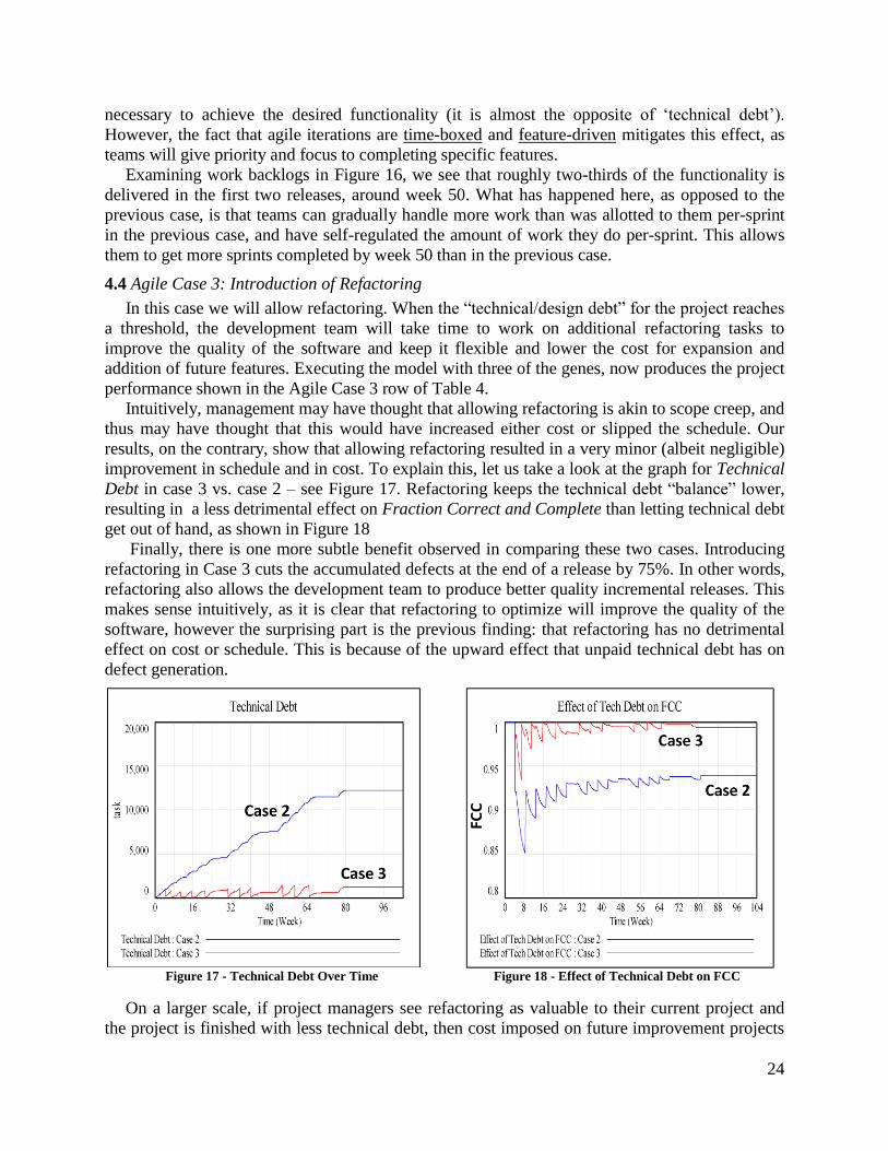
improvement in schedule and in cost. To explain this, let us take a look at the graph for Technical
Debt in case 3 vs. case 2 – see Figure 17. Refactoring keeps the technical debt “balance” lower,
resulting in a less detrimental effect on Fraction Correct and Complete than letting technical debt
get out of hand, as shown in Figure 18
Finally, there is one more subtle benefit observed in comparing these two cases. Introducing
refactoring in Case 3 cuts the accumulated defects at the end of a release by 75%. In other words,
refactoring also allows the development team to produce better quality incremental releases. This
makes sense intuitively, as it is clear that refactoring to optimize will improve the quality of the
software, however the surprising part is the previous finding: that refactoring has no detrimental
effect on cost or schedule. This is because of the upward effect that unpaid technical debt has on
defect generation.
Figure 17 - Technical Debt Over Time Figure 18 - Effect of Technical Debt on FCC
On a larger scale, if project managers see refactoring as valuable to their current project and
the project is finished with less technical debt, then cost imposed on future improvement projects

25
will be much lower. On small projects, the effect of technical debt may not be enough to have any
immediate impact, though again long term effects will accumulate and may overwhelm a future
project.
4.5 Agile Case 4: Introduction of Continuous Integration
Next the Continuous Integration lever is activated. This will increase load in tasks to be
performed, representing the initial effort to set up and configure the development and delivery
environment. Later, once that environment is available and automated tests begin to accumulate,
Continuous Integration enhances productivity, and the ability to detect rework tasks by automated
testing. Executing the model with these parameters produces the project performance results in
the Agile Case 4 row of Table 4.
Figure 19 – Agile Case 4 Quality
There are no surprises here: Introducing Continuous Integration increases cost somewhat, due
to the up-front investment to configure such an environment. However, the cost is recouped in
schedule time. The project duration is shortened thanks to a significant speed-up in rework
discovery. If the project were extended beyond 104 weeks to several years, this up-front cost
becomes less significant. Another interesting observation with this gene is the quality profile as
exhibited in Figure 19.
Compared to what was seen in cases 2 and 3, the quality profile shows that defects have a short
life, as they are quickly discovered and addressed. This has several positive effects. Chiefly: the
“Errors upon Errors” dynamic is less powerful, since there are fewer undiscovered rework tasks
dormant in the system at any given time.
4.6 Summary of Experiments and Comparison with Experience
Table 4 shows the results of experiments described above – the Single-Pass Waterfall base
case and the four Agile cases that each add one more Agile gene. From these experiments, it is
clear that Agile can produce substantially improved performance or can lead to worse
performance, depending on what form of Agile is implemented. For example, the Refactoring
gene adds extra work in the short term to pay down “technical debt” and save work later (often on
a subsequent project). That extra work can be compensated by the “Continuous Integration” gene
which accelerates rework discovery.
Quality (Defects in Product)
100 task
1 Dmnl
50 task
0.5 Dmnl
0 task
0 Dmnl
0 16 32 48 64 80 96
Time (Week)
Defects task
Project Finished Dmnl
Project End

26
Case Schedule (weeks)
Cost (tasks)
Quality (level)
Base Case 0: Single-Pass Waterfall 79 250,223 L
Agile Case 1: Iterative-Incremental 95 275,111 M
Agile Case 2: add Micro-Optimization 82 244,436 M
Agile Case 3: add Refactoring 81.6 243,904 M
Agile Case 4: add Continuous Integration 62.8 255,593 H Table 4 - Summary of Experimental Results
Experimentation with the APD has led to better understanding of some of results observed by
one of the author’s personal experience with Agile. This author reports that during the times when
some form of Agile development was practiced, there was never a case where all seven of the
Agile genes were employed. Customer Involvement was never truly practiced. In one project a
System Engineer (SE) filled the role of customer proxy, and was either unwilling or unable to
participate in daily scrums. Moreover, there is no guarantee that an SE could really represent the
vision of the end user. Continuous Integration was also not truly practiced. Although automatic
unit-testing was used, very little else was automated. Functional tests were still long and laborious
procedure-driven tasks. Configuration Management policy was also isolationist: in other words,
pieces of functionality were developed in isolation and only integrated (“merged”) near the end of
the development cycle, thus no “continuous” aspect of integration to identify rework early.
Refactoring (at least, large-scale refactoring) was also a frowned-upon practice. It was
considered by managers who did not understand the concept of Technical Debt to be extra non-
value-added work. The net result was that in most of this author’s experience with Agile, the only
elements employed were the Feature-Driven, Iterative-Incremental, and Micro-Optimizing genes.
The observed results of a natural experiment in the author’s personal experience are shown in
Table 5
Case Schedule (weeks)
Cost (tasks)
Quality (tasks)
Base Case 79 250223 L
“Personal” Agile Case 82 242213 M Table 5 - APD Project Performance for “Personal” Case
These results are consistent with Agile Case 2 above. As we can see, this configuration saves
some cost, improves quality, and yet delays the project by three weeks. This is by no means a win
for agile over waterfall, or grounds to declare one superior to the other. Depending on program
priorities, schedule may be the most important factor. However this explains a bit more about the
promise and reality of agile practices.
5. Conclusions and Future Research
We have presented the Agile Genome, a unifying framework for describing characteristics of
Agile software development management practices. The framework has been used both to show
the commonalties and differences in popular methodologies and to indicate other combinations of
practices which may be employed. We have found the Agile Genome useful in the development
of the APD model for software development projects, which is capable of simulating both Agile
and Waterfall methodologies. The modular architecture of APD is such that any of the Agile Gene
sub-models can be evolved and refined over time as we gain more insight through personal

27
experience, research and interviews with subject matter experts and software engineering
professionals.
A Systems Thinking perspective would suggest that the software product itself is part of the
system under study here, in addition to the people, processes, and tools and the interactions
thereof that we are trying to model. Holistically speaking, one could argue that true Agile is not
only about the agility of the development process, or the team, but also about the software product
itself. If the software code is constantly refactored to keep it easy to adapt and evolve along with
the requirements, needs, or market environment, then the project can truly be agile. This is one of
the notions that APD helps us explore, thanks to the Refactoring gene sub-model, which includes
a construct for the metaphor of Technical Debt.
The model also gives us insight into the reason why the adoption of Agile in the large-scale
software engineering world has yet to reap the full benefits of Agile: Experiments with the APD
suggest that, for projects to gain the full benefits of Agile, they cannot simply cherry-pick easy-to-
adopt development techniques and hope to derive positive project performance results. We have
learned that each practice, combined with project policies, can produce both positive and negative
effects on the project performance. However, in reality organizations are quick to adopt practices
such as the Daily Scrum but will not practice Refactoring, or have not been able to adopt cutting-
edge Continuous Integration practices. As such, they see little ROI from Agile adoption to date.
The selection of management policies and combination of agile practices by software
development organizations needs to be balanced to optimize the system. Combinations of Agile
genes counter-balance negative effects with positive effects. For example: incremental
development can lead, over time, to high technical debt with negative consequences on
development time and quality. This effect can be counter-balanced by practicing refactoring.
Similarly, the loss in productivity from refactoring can be counter-balanced by gains from the
continuous integration and automated testing.
The goal for management is to configure the project-system in a fashion that maximizes the
up-sides while minimizing the downsides of methods. This underscores the Systems Thinking
adage that “a system is not a sum of its parts, but a product of their interactions”. The APD model
assists in the study of the interactions of the various “parts” of Agile and understanding of the
pluses and minuses of using any combination of methods. The APD’s management dashboard can
act as a “flight simulator” to facilitate this exploration.
By decomposing the Agile concept into component genes, some of the difficulties with
adoption in the government sector become more clear. There are many stakeholders (such as
program sponsors, contracting managers, program managers, and contractors) each of which has
its own perspectives, power, authority, and sense of urgency about any project. Some of the Agile
genes fall almost completely within the domain of the contractor (e.g. pair programming and team
meeting practices). Some are shared responsibility (e.g., incremental releases and customer
involvement). Some practices run contrary to traditional program control processes (such as risk
aversion to any change or rework vs. accepting change as inevitable and maximizing value).
Some Agile practices (such as customer involvement) would require new cooperation between
government and contractors (the government by allowing customers to influence requirements
changes during the project and the contractor by not taking advantage of customer contact to
demand excessive cost increases). The APD model can assist in developing collaborative change
by helping all parties to test the effects of new policies before they are put in place.
The APD model is explicitly designed to evolve as more is learned about Agile methods and
other aspects of project management. By substituting a more complete staffing model, for

28
example, we have been able to investigate how Agile practices respond to budget gaps and
fluctuations on software projects[34], and whether Agile projects are more resilient to such
funding problems. We expect to continue to test and evolve the Agile Genome framework and
extend the model to management practices that guide the definition and prioritization of features
for software development and to the interaction of software product with users.
References [1] n.d., “Waterfall model,” Wikipedia. [Online]. Available: http://en.wikipedia.org/wiki/Waterfall_model.
[Accessed: 02-Aug-2012].
[2] K. Beck et al. (2001), “Manifesto for Agile Software Development,”[Online]. Available:
http://agilemanifesto.org.
[3] C. Larman and V. Basili (2003), “Iterative and Incremental Development: A Brief History,” Computer, vol. 36,
no. 6, pp. 47-56..
[4] B. Berwin (2010), “How a lawn mowing contract is changing Defense acquisition,” NEXTGov, pp.1-2.
Available at: http://www.nextgov.com/nextgov/ng_20100916_6260.php.
[5] C. Argyris and D. Schon (1978), Organizational Learning: A theory of action perspective. Reading, MA:
Addison-Wesley.
[6] P. Deemer, G. Benefield, C. Larman, and B. Vodde (2009), “The Scrum Primer.” Scrum Foundation, pp. 1-22.
[7] T. J. Allen and G. Henn (2006), The Organization and Architecture of Innovation: Managing the Flow of
Technology. Taylor & Francis..
[8] B. W. Boehm and P. N. Papaccio (1990), “Understanding and Controlling Software Costs,” IEEE Transactions
on Software Engineering, vol. 14, pp. 1462-1477..
[9] V. Basili and F. Shull (2005), “Evolving Defect ‘Folklore’: A Cross-Study Analysis of Software Defect
Behavior,” in International Software Process Workshop, pp. 1-9.
[10] M. A. Cusumano and S. Smith (1995), “Beyond the Waterfall: Software Development at Microsoft,” MIT Sloan
School of Management WP# 3844-BPS-95.
[11] J. M. Lyneis, K. G. Cooper, and S. A. Els (2001), “Strategic management of complex projects: a case study
using system dynamics,” System Dynamics Review, vol. 17, no. 3, pp. 237-260.
[12] T. K. Abdel-Hamid and S. Madnick (1991), Software Project Dynamics: An Integated Approach. Prentice Hall..
[13] C.H. Fine (1996), “Industry Clockspeed and Competency Chain Design,” MIT Sloan School of Management
Working Paper No. 147-96.
[14] Armed Forces Communications and Electronics Association (AFCEA 1982), Command & Control (C2)
Systems Acquisition Study Final Report. Washington, DC: Defense Technical Infor Center, Sept. 1982.
[15] L. M. Duvall (2012), "Be Quick, Be Useable, Be On Time: Lessons in Agile Delivery of Defense Analytic
Tools," Brookings Center for 21st Century Security and Intelligence Policy Paper, June 6, 2012.
[16] J. Highsmith (2002), “What Is Agile Software Development?” CrossTalk. The Journal of Defense Software,
(October 2002). Available at:
http://scholar.google.com/scholar?hl=en&btnG=Search&q=intitle:What+Is+Agile+Software+Development+?#
0 [Accessed April 18, 2012].
[17] Defense Science Board. (2009) “Department of Defense Policies and Procedures for the Acquisition of
Information Technology” Office of the Under Secretary of Defense for Acquisition, Technology, and Logistics:
Washington, DC, (March 2009).
[18] W. Cunningham (1992), “The WyCash Portfolio Management System,” OOPSLA ’92 Experience Report.
[19] I. McFarland (2006), “Agile Practices on Real-World Projects.” In Google Java Users Group Agile 101.
[20] L. Cao, B. Ramesh, and T. Abdel-Hamid. (2010). “Modeling dynamics in agile software development.” ACM
Trans. Manage. Inf. Syst. 1, 1, Article 5 (December 2010)
[21] K. Chichakly (2007). "Modeling Agile Development: When Is It Effective?" Proc Int’l Conf. of the System
Dynamics Society 2007.
[22] W. Tignor (2009), “Agile Project Management,” Proc. Int’l Conf. of the System Dynamics Society 2009.
[23] K. van Oorschot, K. Sengupta and Luk van Wassenhove (2009), “Dynamics of Agile Software Development,”
Proc. Int’l Conf. of the System Dynamics Society 2009
[24] W. Tignor (2011), “Agile Essence,” Proc. Int’l Conf. of the System Dynamics Society 2011.
[25] X. Kong, L. Liu and J, Chenc'a. (2011) “Modeling Agile Software Maintenance Process Using Analytical
Theory of Project Investment,” Procedia Engineering, Volume 24.
29
[26] S. Marjaie and U. Rathod (2011) “Communication in Agile Software Projects: Qualitative Analysis using
Grounded Theory in System Dynamics,” Proc. Int’l Conf. of the System Dynamics Society 2011.
[27] L. Cocco, K. Mannaro, G. Concas, and M. Marchesi (2011). "Simulating Kanban and Scrum vs. Waterfall with
System Dynamics", XP 2011.
[28] K. Cooper and T. Mullen (1993), "Swords and Plowshares: The Rework Cycle of Defense and Commercial
Software Development". American Programmer Vol 6, no. 5, (May 1993).
[29] D. West, et al. (2010). “Agile Development: Mainstream Adoption Has Changed Agility.” Forrester Research.
[30] D. West et al. (2011) “Water-Scrum-Fall Is The Reality Of Agile For Most Organizations Today.” Forrester
Research.
[31] F. Brooks (1975) The Mythical Man-Month. Addison-Wesley.
[32] M. Lapham, et al. (2010) “Considerations for Using Agile in DoD Acquisition.” Carnegie Mellon, Software
Engineering Institute: April 2010, Technical Note CMU/SEI-2010-TN -002.
[33] Rico, D. F. (2008). "What is the return of investment (ROI) of agile methods?": 7
[34] T. Trammell, S. Madnick and A. Moulton (2012), "Effect of Funding Fluctuations on Government Funded
Software Development," International Research Workshop on IT Project Management 2012. Paper 12.
Acknowledgments The authors would like to thank Mr. Richard Herrick, Mr. Kelly Hughes, Ms. Sarah Kingensmith, and Mr. Ian
Macurdy at the Defense Intelligence Agency and Mr. Douglas Marquis at MIT Lincoln Labs, for their valuable
insights into the issues addressed in this paper. The work reported herein was supported, in part, by the MIT Lincoln
Laboratories and the Defense Intelligence Agency (DIA) under the "Understanding the Challenges to Net-Centric
Systems and Mitigating Approaches" project, MIT Lincoln Laboratory contract 16-11-TCO-0013. Any opinions,
findings, and conclusions or recommendations expressed in this material are those of the authors and do not reflect
the official policy or position of Raytheon, MIT Lincoln Laboratory, the Defense Intelligence Agency or the
Department of Defense.