MNRAS 000, 000–000 (0000) Preprint July 31, 2020 Compiled using MNRAS LATEX style file v3.0

AGN dichotomy beyond radio loudness: a Gaussian MixtureModel analysis

Pedro P. B. Beaklini,1,2Allan V. C. Quadros,3,4 Marcio G. B. de Avellar,5,6Maria L. L. Dantas,1 André L. F. Cançado31Instituto de Astronomia, Geofísica e Ciências Atmosféricas, Universidade de São PauloRua do Matão 1226, 05508-090, São Paulo/SP, Brazil.2National Radio Astronomy Observatory1003 Lopezville Road, Socorro, NM 87801, United States of America3Departamento de Estatística, Universidade de Brasília, UnBCampus Universitário Darcy Ribeiro, Sgan, Asa Norte, 70910-900, Brasília-DF, Brazil4Department of Statistics, Kansas State University101 Dickens Hall, 1116 Mid-Campus Drive N., Manhattan KS 66506-0802, United States of America5Instituto Tecnológico de Aeronáutica, CTAPraça Marechal Eduardo Gomes, 50, Vila das Acácias, 12228-900, São José dos Campos/SP, Brazil6 Departamento de Física, Universidade Federal de São PauloRua São Nicolau 210, 09913-030, Diadema/SP, Brazil

July 31, 2020

ABSTRACTSince the discovery of Quasi-stellar Objects (QSOs), also known as quasars, they havebeen traditionally subdivided as radio-loud and radio-quiet sources. Whether such di-vision is a misleading effect from a highly heterogeneous single population of objects,or real has yet to be answered. Such dichotomy has been evidenced by observations ofthe flux ratio between the optical and radio emissions (usually B-band and 5 GHz).Evidence of two populations in quasars and samples of a wide diversity of AGNs hasbeen accumulated over the years. Other quantities beyond radio loudness also seem toshow the signature of the existence of two different populations of AGN. To verify theexistence of a dichotomy through different parameters, we employed a soft clusteringscheme, based on the Gaussian Mixture Model (GMM), to classify these objects si-multaneously using the following parameters: black hole mass, colour and R loudnessindex, as well as the usual radio and B-band luminosity. To investigate whether dif-ferent kinds of AGNs manifest any population dichotomy, we applied GMM to fourindependent catalogues composed of both optical and radio information. Our resultsindicate the persistence of a dichotomy in all datasets, although the discriminatingpower differs for different choices of parameters. Although the Radio Loudness pa-rameter alone does not seem to be enough to display the dichotomy, the evidenceof two populations of AGNs could persist even if we consider other parameters. Ourresearch suggests that the dichotomy is not a misleading effect but real.

Key words: (galaxies:) quasars: general – galaxies: active – Astronomical Data bases– methods: data analysis

1 INTRODUCTION

It is well known that there are different types of AGNs andthat most of the diversity can be explained as a consequenceof the angle between the source structures and the line ofsight, following the AGN unification schema (e.g., Holt et al.1992; Antonucci 1993; Urry & Padovani 1995; Peterson 1997;Ho 2008). However, it is also well known that there are someintrinsic differences between the AGN like the core or lobedominated Fanaroff–Riley galaxies (Fanaroff & Riley 1974),

the black hole spin (Moderski et al. 1998; Brenneman 2013;Barret & Cappi 2019; Unal & Loeb 2020), the accretionrate of the central engine (Bian & Zhao 2002; Körding et al.2008; Daly et al. 2018), and the radio to optical luminos-ity relation (Kellermann & Pauliny-Toth 1966; Murdoch &Crawford 1977; Condon et al. 1980; Kellermann et al. 1989).The last point is known in the literature as the radio-loudand radio-quiet quasar dichotomy, being the first evidence

c© 0000 The Authors

arX

iv:2

007.

0727

1v2

[as

tro-

ph.G

A]

29

Jul 2

020

2 Pedro P. B. Beaklini

of the existence of two inherently different populations ofAGNs (see Peterson 1997).

The existence of a dichotomy involving the radio emis-sion of quasars is a long-lasting question since the discoveryof the Quasi-Stellar Radio Sources, known as quasars, inthe ’60s. From the total well-known Quasi-Stellar Objects(QSOs) sample at that time, almost 10% of them were de-tected at radio wavelengths and classified as quasars (Chiu1964; Kellermann & Pauliny-Toth 1966; Shapiro & Weinreb1966; Katgert et al. 1973; Fanti et al. 1977), and only a fewof them were classified as radio-loud sources. These pecu-liarities indicate that radio properties could be fundamentalto classify active galactic nuclei (AGNs), which led to thefirst division between Radio-Loud and Radio-Quiet objects(see Kellermann et al. 1989). However, whether this disjunc-tion is physical or statistical is unclear (see, e.g., Kellermannet al. 2016, and references therein).

Kellermann et al. (1989) defined the radio loudness pa-rameter (R) as an indicator of whether the source is radio-quiet or loud. The authors suggested a comparison betweenthe radio and optical B-band fluxes; a source was definedas radio-loud (hereafter RL) when the radio flux was higherthan the B-band, and radio-quiet (hereafter RQ) otherwise.It is worthwhile noticing two aspects of analysing BL Lacand flat-spectrum radio quasars (FSRQ): (i) the beamingeffect increases in different ways for the fluxes in radio andoptical wavelengths; (ii) opacity effects are a source of biases(for instance, see Blandford & Königl 1979; Urry & Padovani1995; Falcke et al. 1996b). By taking these issues into ac-count, the R parameter is the commonly adopted criterionused to classify a source as radio-loud or quiet. Although itis a very useful criterion, other works suggest different crite-ria to look for a more evident dichotomy (e.g., Van Gorkomet al. 2015).

It is essential to discuss the meaning of a real dichotomy.Notably, some AGNs are bright at radio wavelengths whileothers are not (e.g., Chiu 1964; Scheuer & Readhead 1979;Smith & Wright 1980; Sramek & Weedman 1980; Strittmat-ter et al. 1980). Naturally, this statement is also valid atother wavelengths. It is also well known the existence ofexternal factors that increase the continuum emission thatdepends on the jet position relative to the line of sight; thewell-known beaming effect is one of them (Rees 1966; Bland-ford & Königl 1979). Therefore, the question to be addressedis: is there a continuous change of the brightness throughoutthe AGN population? Is this evident only when we look atthe number of quasars versus the radio loudness parameter?Or are there other types of AGNs where a dichotomy couldbe seen in other parameter spaces? We can also pose thesequestions in another way. Can other parameters evidence adichotomy?

First, let us take into account only the radio loudnessdichotomy (that we will call hereafter of the traditionalRL/RQ dichotomy). In general, two main approaches tryto find the existence of two populations. The first one is tosearch directly for a gap in the bright luminosity and the Rparameter space. The second is to try to determine the dis-tribution of radio flux between RQ and RL sources to showthat they are not compatible with just one general distri-bution (e.g., Strittmatter et al. 1980; Falcke et al. 1996a;White et al. 2000; Cirasuolo et al. 2003b; Sikora et al. 2007;Broderick & Fender 2011; Mahony et al. 2012; Kellermann

et al. 2016). Both are limited by a two-parameter analy-sis, although Sikora et al. (2007) and Broderick & Fender(2011) also used the central source mass to investigate thebimodality.

In the context of the first approach, Sikora et al. (2007)found two parallel tracks in the luminosity plot. We high-light that the authors constructed a catalogue with sourcesof different types, expanding the original idea of quasardichotomy: Broad-line radio galaxies, radio-loud quasars,Seyferts, LINERs, quasars, and FR I galaxies. Using thesame catalogue, but considering only the core flux, Broder-ick & Fender (2011) used the black hole fundamental plane(Merloni et al. 2003; Falcke et al. 2004) to investigate howthe mass could affect the traditional RL/RQ dichotomy. Theauthors concluded that the gap previously found by Sikoraet al. (2007) was still present after the mass correction, butnot as evident as before.

On the other hand, observations made by the Faint Im-ages of the Radio Sky at Twenty survey (FIRST, Beckeret al. 1995; White et al. 1997, 2000) provided an extensivedatabase. The instrument used was the Very Large Array(VLA) at 1365 and 1435 MHz. It provided flux measure-ments of a large number of sources that would be ideal forverifying the existence of different populations. However, thedata from the FIRST catalogue did not reveal two differentpopulations of radio sources (White et al. 2000; Lacy et al.2001; Cirasuolo et al. 2003b,a; Wals et al. 2005; Rafter et al.2009; Singal et al. 2011; Bonchi et al. 2013). Besides, anal-yses based on ATCA (Australia Telescope Compact Array)and the ROSAT (Röntgensatellit) All-Sky Survey did notfind evidence of two intrinsically different classes of QSOs(Mahony et al. 2012).

Kellermann et al. (2016) pointed out that the lack ofdetection on the FIRST catalogue could be a consequence ofthe large antenna beam at its frequency. In other words, theantenna detected not only the core emission but also the lobeemission, which could introduce noise to the distribution.Nevertheless, the authors also argued that the X-ray QSOcatalogue (Mahony et al. 2010) favoured blazars and thatthe ATCA sensibility could hide the RQ population.

Kellermann et al. (2016) have also used VLA obser-vations of SDSS. They used the QSOs sample presented byKimball et al. (2011) at 6 GHz, which was based on the com-pilation by Schneider et al. (2010). The authors restrictedtheir data in a very narrow redshift interval between z = 0.2and z = 0.3, which made it impossible to confirm whetherthe redshift evolution exists. However, they revealed a bi-modal distribution not found in Kimball et al. (2011). Wehighlight that the authors confirmed the definition of thetraditional dichotomy, which is well-described through theradio loudness parameter and in a sample formed only byquasars.

Now, let us go through other parameters. In an attemptto perform a multi-dimensional analysis and try to solve ifa dichotomy could be seen in other wavelengths, Sulenticet al. (2015) used the eigenvector correlation space consid-ering line parameters in optical and UV range beyond theX-ray photon index (Sulentic et al. 2000). The authors foundthat radio-loud sources are restricted to a small group com-pared to the whole population of radio quasars. A potentialcause for this cleavage was suggested to be quasar evolution(Schoenmakers et al. 2000; Best & Heckman 2012). Some au-

MNRAS 000, 000–000 (0000)

AGN dichotomy beyond radio loudness: a Gaussian Mixture Model analysis 3

thors considered quasar luminosity evolution when search-ing for dichotomy (Singal et al. 2013). Retana-Montenegro& Röttgering (2017) investigated the existence of quasars’spatial clustering and detected significant correlations withredshift for RL quasars at z ≤ 2.3, which could provide valu-able information about quasar evolution. The dichotomy inquasars seems to be a general property, and not only a con-sequence of the radio emission.

In the context of a multi-parametric analysis, Singalet al. (2013) described the luminosity evolution of radio andoptical emission of quasars combining Sloan Digital Sky Sur-vey (SDSS) sources and the FIRST catalogues. The authorsapplied a multi-dimensional correlation method of Efron &Petrosian (1992) to take into account flux limitations andsample restrictions. They did not find evidence for bimodal-ity, but this could be a consequence of the FIRST limitationsmentioned above.

To evaluate the extent of a dichotomy among AGNs,we studied a set of features from different papers and cata-logues by using a probabilistic methodology. Therefore, weemployed a Gaussian Mixture Model (see de Souza et al.2017) to this multi-parametric space in order to: (i) testwhether a dichotomy exists beyond the radio flux; (ii) if so,to find the best combination of parameters to discriminatethem, and (iii) search if the dichotomy is presented evenin samples with more AGN diversity than quasars. In thissense, we are not restricting to the radio emission dimen-sion but taking an overall look at the possible dichotomiesin AGNs.

Thus, in summary, we are searching for a dichotomyalong many possible surfaces in the space of quasar parame-ters, only one of which is the traditional RL/RQ dichotomy,which has received a lot of previous attention in the litera-ture.

In the next section, we present the samples we used. Insection 3, we discuss the importance of this multi-parameteranalysis in astronomy and the method we used, while insection 4, we show our results. We discuss our results insection 5, and we conclude in section 6.

2 DATA RETRIEVAL

The multi-dimensional analysis of the radio sources’ emis-sions can help to determine the reliability of an AGN di-chotomy. Even the traditional RL/RQ dichotomy is still un-der debate. Different samples and analyses point many timesto contradictory results. In this work, we will not compile anew database since there are already many of them in theliterature, as pinpointed in section 1. Instead, we will usedifferent samples to investigate how the dichotomy appearsin other observational parameters.

In other words, we did not compile any new database;we used in this work the databases compiled and treated bythe authors cited in Table 1. We did not modify or treatany data; we only normalised the data in the way describedbelow.

We now have different questions to address since weare working with parameters other than the radio and theB band luminosities and with a broad class of AGNs. Isthe dichotomy a general property? Do the two populationsappear when we use a comprehensive set of parameters?

Does the dichotomy appear through different classes of AGNbeyond quasars?

The main problem of thinking in a multi-dimensional ormulti-parameter analysis is to define which parameter spaceis the best one to investigate. In an ideal scenario, we wouldhave a big catalogue with several well-determined param-eters, but this is not the case. The catalogues containingSDSS information, for example, do not have the mass of thecentral source for most of the sources, while some objectsof the FIRST catalogue do not have an optical counterpart.Then, choosing a sample is choosing the parameters worthyof investigating.

Our goal is to introduce the multi-dimensional proba-bilistic analysis in the discussion. We selected four datasetsused in previous works as follows.

(i) Original database compiled by Sikora et al. (2007);(ii) The modified version of the Sikora et al. (2007)

database by Broderick & Fender (2011);(iii) The sample of Schneider et al. (2010) and Kimball

et al. (2011) also analysed by Kellermann et al. (2016);(iv) The FIRST data used by White et al. (2000).

In the following, we briefly describe each sample indi-vidually.

Dataset D1 (5 GHz, B-Band, Mass, R): There are 198objects in this sample. The authors made use of the fol-lowing parameters: 5 GHz radio flux, B-band, mass, andRadio Loudness parameter. The disadvantages of includingthe black hole mass, as performed by Sikora et al. (2007),is the low number of well-known sources; it limits the to-tal number of entries in the catalogue. Nonetheless, the au-thors correctly excluded blazars because of the boosting oftheir emission. Five classes of sources were obtained fromdifferent catalogues considering radio emission (Schmidt &Green 1983; Eracleous & Halpern 1994, 2003), radio struc-ture (Woo & Urry 2002; Cao & Rawlings 2004; Kharb &Shastri 2004), and Seyferts and LINERs (Ho & Peng 2001;Ho 2002). Sikora et al. (2007) discussed the details of eachsub-sample. This sample provides a space of parameters con-taining Radio and optical luminosity, the R parameter, andthe black hole mass, with a total of 198 sources.

Dataset D2 (5 GHz core, B-Band, Mass, R): Thereare 198 objects in this sample. The authors made use of thefollowing parameters: 5 GHz radio core flux, B-band, mass,and radio core Loudness parameter. Broderick & Fender(2011) also used this compilation to analyze the influence ofthe black hole’s fundamental plane on the dichotomy. How-ever, Broderick & Fender (2011) applied a correction on theoriginal sample radio flux to guarantee that the used fluxcorresponded to the core emission, which changes not onlythe radio luminosity but also the R parameter.

Dataset D3: (Offset, 6 GHz, B-Band, R) There are 178objects in this sample. The authors obtained the followingparameters: 6 GHz Radio Flux, B-Band, Radio Loudness pa-rameter, and displacement between radio and optical emis-sion. From the sample analysed by Kellermann et al. (2016)and compiled by Kimball et al. (2011), the authors used onlya small range of redshift (between 0.2 and 0.3) to avoid the

MNRAS 000, 000–000 (0000)

4 Pedro P. B. Beaklini

influence of evolutionary effects and used a rigorous selec-tion criterion based on colours, magnitude (which excludeslow luminosity AGNs), and the presence of broad lines (atleast one). The final list had 178 SDSS quasars. The sampleprovides information about the luminosities at radio and Ibands, the offset between radio and optical emission, the Rparameter, and the redshift.

Dataset D4: (1.4 GHz,B-Band, R-Band, colour (B-Rb)) There are 636 objects in this sample. The authors ob-tained the following parameters: 1.4 GHz Radio Emission,B-band, R-band (representing as Rb), andRLoudness pa-rameter. The fourth and last sample we used in this workwas based on the FIRST catalogue. No dichotomy has beenreported in this dataset, although reasons for the lack of de-tection exist, as discussed in section 1. Our goal is to verifywhether a probabilistic multivariate method like GMM canindicate some new information even at this beam resolution.

We stress that all samples have already been accountedfor the K-correction and that sources with strong beam-ing effects were not considered. Nonetheless, Falcke et al.(1996b) showed that the boosting effect could affect evenRQ sources, but Broderick & Fender (2011) argued that itis not a crucial matter for the Sikora et al. (2007) sampling,while Kellermann et al. (2016) ruled out the Doppler boost-ing as the origin of the dichotomy.

For all samples, we first took the logarithm of the valuesof each parameter. Then, we scaled the new values from 0to 1 by the formula below, where min and max representthe minimum and maximum value of each parameter:

f(x) =(x−min)

(max−min) .

We emphasise that the scaling does not affect the mainresults. This procedure’s objective is to avoid that any localminimum in the statistical method blurs the result. We alsoused this normalised scale on our plots.

To investigate the existence of a dichotomy, we also needto discuss a suitable approach concerning the outliers of eachsample. Notice that since we are trying to identify a sup-posed second population, this second population could beprecisely a group of outliers. After removing entries belowthe 5th percentile and above the 95th percentile, the num-ber of sources may decrease significantly; thus, the outliersare the points that fall outside the 5-95 percentile range forany parameter. We present and discuss both results – withand without the outliers – and deliberate on both results.

At this point, we must emphasize that the definitions ofradio-loud and radio-quiet may not be enough to interpretthe groups we find. Since we are now dealing with a multi-parameter space, the groups do not necessarily correspondto the RL or RQ groups.

3 METHODOLOGY

This section briefly describes the methodology chosen toaddress the issue involving different clusters of QSOs. Weemployed a probabilistic approach known as the Gaussian

Mixture Model (GMM) to evaluate the presence of differentclusters or groups in each dataset.

A Mixture Model is defined as a probability densityfunction comprised of a weighted summation of componentdensities. Therefore, in the GMM, we have a summation ofGaussian Components (GC), in which each of these GCsindicates one potential cluster in the data (McLachlan &Peel 2000; Hastie et al. 2001; Mengersen et al. 2011; Murphy2012; de Souza et al. 2017; Ucci et al. 2018).

For a total of k components in a d-dimensional param-eter space, one can write the GMM as:

f(x) =

k∑i=1

ζiφ(x;µi,Σi), (1)

with mixture weights denoted by ζi, and∑k

i=1 ζi = 1. Eachof the k components is described as a d-variate Gaussiandensity, fully characterised by its mean µi and covariancematrix Σi, given by:

φ(x;µi,Σi) =1√

(2π)d|Σi|e−

12(x−µi)

′Σ−1i (x−µi). (2)

In this scenario, to each point in the dataset, we assigna probability of membership to each GC. Thus we assign thepoint to the cluster to which it has the highest probability ofmembership after the convergence of the fitting algorithm.Fitting a GMM means estimating the maximum likelihoodfunction of the Gaussian Mixture. The estimation is doneusing the Expectation-Maximization (EM) algorithm. Thismethod consists of a data augmentation procedure with un-derlying data, represented by the model memberships, dur-ing the fitting procedure of a GMM (Hastie et al. 2001;Dempster et al. 1977; McLachlan & Krishnan 2008).

The EM algorithm from the r (R Core Team 2016)package mclust (Fraley & Raftery 2002) is used to fit theGaussian Mixture models to each dataset. Since our goalis to verify whether there is a bimodality in each type ofsource, we fitted solutions for k = 1 and k = 2 clusters.

In order to evaluate whether the results have indicatedor not the presence of a dichotomy, we have employed amodel selection framework along with a hypothesis testingmethodology to evaluate how significant is the hypothesisof having two or more heterogeneous populations in eachdataset.

First, we used the Integrated Completed Likelihood(ICL) criterion (Biernacki et al. 2000) to measure each solu-tion’s goodness of fit. We were able to indicate the presenceor absence of a dichotomy in each parameter space by com-paring the ICL of GMMs with k = 1 and k = 2 groups. Weused the icl() function from the mclust package, where agreater ICL indicates a better model or solution.

The ICL is an alternative to the standard and widelyused Bayesian Information Criterion (BIC) and better suitedto our purposes in this paper. In the context of density es-timation, BIC has a satisfactory performance. However, ittends to overestimate the number of clusters when employedin the model-based clustering analysis context (Biernackiet al. 2000). In our case, this could result in some bias to-wards the k = 2 solutions. Although some authors have usedit to assess the number of clusters in data (Biernacki et al.2000), when some of the regularity conditions for the Normaldistribution are not present, more Gaussian components are

MNRAS 000, 000–000 (0000)

AGN dichotomy beyond radio loudness: a Gaussian Mixture Model analysis 5

Table 1. Summary of samples used in this work

Dataset References Parameters Objects no OutliersD1 (Sec. 4.1) Sikora et al. (2007) 5 GHz, B-Band, Mass, R 197 131D2 (Sec. 4.2) Sikora et al. (2007); Broderick & Fender (2011) 5 GHz (core), B-Band, Mass, Rcore 197 131D3 (Sec. 4.3) Schneider et al. (2010); Kimball et al. (2011) Offset, 6 GHz, B-Band, R 175 116

Kellermann et al. (2016)D4 (Sec. 4.4) White et al. (2000) 1.4 GHz,B-Band, R-Band, (B-Rb) 636 419

fitted to encompass the whole data or a unique cluster, thusoverestimating k. Since our datasets do not follow a normaldistribution, this reinforces our option for the ICL.

A disadvantage of the ICL is that there is no mention tothe significance of the difference between ICL values whencomparing two models, as Raftery (1995) has provided forthe BIC using the Bayes Factor framework. A difference inthe BIC values from two models represents an odds ratiogiven by the probability that the model B is correct giventhe data, over the probability that model A is correct giventhe data. For example, a difference of |10| between two BICsrepresents a 150 : 1 odds ratio that the model with thesmaller BIC is the better fitted one. Considering that theICL formula contains a BIC-like approximation, we can usethis number as a loose reference when comparing ICL valuesfor two solutions.

As a complement to the ICL criterion, we employed ahypothesis-testing framework. Fuentes & Casella (2009) de-veloped a Bayesian procedure to test for the existence ofclusters in a multivariate dataset. The main goal is to testH0 : k = 1 vs H1 : k > 1 . Here, H0 is the null hypothesisand denotes the existence of a unique group (no dichotomy)in the sample. The alternative hypothesis, H1, denotes thepossibility that there is more than one group in the dataand can be simplified to k = kn, where kn is the number ofgroups that we want to test against k = 1. Therefore, themethod allows us to test whether the data represent a sin-gle homogeneous population or two (or more) populations.Since we are interested in evaluating the existence of a di-chotomy, i.e. kn = 2, we tested in favour of H1 : k = 21.Thus, we obtain a measure of the significance of the alter-native hypothesis k = 2. That means we can evaluate if wehave sufficient evidence to reject the hypothesis of a singleand homogeneous population, indicating instead the exis-tence of two separate groups (dichotomy).

In the hypothesis testing framework, the significancelevel, α, is also known as the probability of making a TypeI error, i.e., the probability of wrongly rejecting the null hy-pothesis H0 (Johnson & Bhattacharyya 2006). In our case,it means that we would reject the hypothesis of no groupdivision (k = 1) when, in fact, there are no discrete popula-tions of AGNs. The α significance level is set a priori andwill serve as the base of comparison for our p-value, which isthe probability of observing a value at least as extreme as wehave observed for the test statistic under the null hypothesisdistribution (i.e., assuming that H0 is correct).

We opt for a strict 1 per cent α (i.e., we set α = 0.01)level to evaluate the significance of the hypothesis testingresults. We reject the null hypothesis if the computed p-

1 We used the bayesclust package (Gopal et al. 2012), an r (RCore Team 2016) implementation of the aforementioned method.

value is less than 0.01. Therefore, by setting a small valuefor α, such as one percent, we are very rigorous since wewould only reject the hypothesis of a single AGN population(k = 1) if the p-value is smaller than 0.012. This is equivalentto say that the data have to provide robust evidence so thatwe decide to reject the hypothesis that there is only onehomogeneous population of AGNs.

Therefore, our methodology consists of fitting Gaussianmixture models with k = 2 solutions to each dataset (withand without the outliers); fitting GMMs with k = 1 solutionand comparing ICL values for k = 2 and k = 1 solutions;and, in order to complement the analysis, we evaluate thesignificance of the results by testing against k = 1 (in favourof k = 2), using a hypothesis testing framework.

4 RESULTS

This section describes the results of the application of theGMM to the four catalogues. Each catalogue reflects a dif-ferent space of parameters, hence enabling to test the ro-bustness of a dichotomy prevalence against different galaxyproperties.

In what follows, we describe each GMM fit. It is worthnoting that we performed all analyses in the multivariatespace composed by all parameters of each catalogue, but forvisualisation purposes, we display the projected pair-wisetwo-dimensional solutions.

4.1 D1: parameter space: Radio and B Bands,Mass and R

We shall note that, because this sample presents a broaderdiversity of sources (FR I galaxies, PG quasars, Broad LineRadio galaxies, Seyferts, and LINERS), Sikora et al. (2007)weighted the R parameter by the Eddington Luminosity,which differs from the classical definition commonly appliedto quasars.

We present the GMM fit in the left column of Figure 1.We use different symbols depending on the radio loudnessparameter value to determine the extent to which the groupscorrespond with the traditional RL/RQ dichotomy: crossesindicate sources with R > 1, and circles represent sourceswith R < 1. Colours in the figures represent the best groupdivision we found. The result is that the ICL slightly favoursthe presence of two groups instead of one.

In this same Figure, one can see the 95 and 68 per centconfidence regions limited, respectively, by the outer and

2 The probability of observing the computed test statistic underthe null hypothesis distribution (H0) has to be considerably smallto assume that we are actually dealing with values under theprobability density of the alternative hypothesis (H1).

MNRAS 000, 000–000 (0000)

6 Pedro P. B. Beaklini

0.0

0.6

1.2

0.0 0.6 1.2Radio

B Ba

nd

0.0

0.6

1.2

0.0 0.6 1.2Radio

B Ba

nd

0.0

0.6

1.2

0.0 0.6 1.2Radio

Mas

s

0.0

0.6

1.2

0.0 0.6 1.2Radio

Mas

s

0.0

0.6

1.2

0.0 0.6 1.2Radio

R

0.0

0.6

1.2

0.0 0.6 1.2Radio

R

0.0

0.6

1.2

0.0 0.6 1.2B Band

Mas

s

0.0

0.6

1.2

0.0 0.6 1.2B Band

Mas

s

0.0

0.6

1.2

0.0 0.6 1.2B Band

R

0.0

0.6

1.2

0.0 0.6 1.2B Band

R

0.0

0.6

1.2

0.0 0.6 1.2Mass

R

0.0

0.6

1.2

0.0 0.6 1.2Mass

R

Cluster 1 2

Ratio R < 1 R >= 1

Figure 1. GMM results for the space of parameters for datasetD1 (parameters 5 GHz flux density, B-Band magnitude, Mass, Rindex ), where the circles indicate a confidence interval of 95 and68 per cent. On left: the whole sample. On right: After removingthe outliers.

0.0

0.6

1.2

0.0 0.6 1.2Radio

B Ba

nd

0.0

0.6

1.2

0.0 0.6 1.2Radio

B Ba

nd

0.0

0.6

1.2

0.0 0.6 1.2Radio

Mas

s

0.0

0.6

1.2

0.0 0.6 1.2Radio

Mas

s

0.0

0.6

1.2

0.0 0.6 1.2Radio

R0.0

0.6

1.2

0.0 0.6 1.2Radio

R0.0

0.6

1.2

0.0 0.6 1.2B Band

Mas

s

0.0

0.6

1.2

0.0 0.6 1.2B Band

Mas

s

0.0

0.6

1.2

0.0 0.6 1.2B Band

R

0.0

0.6

1.2

0.0 0.6 1.2B Band

R

0.0

0.6

1.2

0.0 0.6 1.2Mass

R

0.0

0.6

1.2

0.0 0.6 1.2Mass

R

Cluster 1 2

Ratio R < 1 R >= 1

Figure 2. GMM results for the space of parameters for datasetD2 (parameters 5 GHz core flux density, B-Band magnitude,Mass, R index ), where the circles indicate a confidence inter-val of 95 and 68 per cent. On left: the whole sample. On right:After removing the outliers.

MNRAS 000, 000–000 (0000)

AGN dichotomy beyond radio loudness: a Gaussian Mixture Model analysis 7

inner ellipses. These regions are related to the estimatedpopulation parameters after fitting the Gaussian mixturesand should not be confused with a quantile region for thesample. To illustrate their meanings, let us take the 95 percent region as an example. It indicates that if we were toreplicate the sampling from the underlying fitted distribu-tion as many times as possible, and for each replication wecompute the confidence region, then 95 per cent of the el-lipses constructed this way would contain the real mean ofthe population. Likewise, for the inner ellipses, 68 per centof the intervals ellipses so constructed would contain theunderlying mean.

Based on the R > 1 distribution in the groups, itwould be possible to find a correspondence between themulti-parameter dichotomy and the traditional RL/RQ di-chotomy: In one group, there are 80 sources R > 1, and nosources with R < 1, and then this could be the correspon-dence with the RL population. However, the total numberof R > 1 is 143 sources. Our multi-parameter analysis indi-cates that 63 sources known as RL would be better classifiedtogether with the RQ, in opposition to the criterion of usingthe weighted R parameter.

We should note that Sikora et al. (2007) defined the Rparameter estimating the bolometric luminosity. We agreethat this redefinition of the R parameter has the advantageof expanding it to other AGNs, but maybe to use it, we needto think about the dichotomy concept more broadly. More-over, the group classification we found seems to have a cleardivision at normalised radio flux of 0.75, indicating that inour RL definition, the radio luminosity could be used as afundamental quantity to the dichotomy without the need tocompare with any other luminosity. Nonetheless, using thewhole sample, we did not find the same dichotomy as foundby Sikora et al. (2007), in which the sources followed two dif-ferent and parallel tracks on the plane between radio and Bluminosities (see left column). However, when we remove theoutliers, the parallel tracks appear as a natural division be-tween the groups. In this approach, the total sample has 131sources. The group in blue (Figure 1), which has more RadioLoud sources, has a total of 46 sources. It seems very sim-ilar to the traditional RL/RQ dichotomy that Sikora et al.(2007) have found.

This indicates that, at least for this weighted R parame-ter, the loudness parameter only makes the dichotomy clearif we remove the most extreme objects. In this case, the ex-istence of two parallel tracks in all the planes is remarkable,as shown in the right column of Figure 1. In section 5, wediscuss the contribution of each parameter. Nonetheless, thedetection of a dichotomy using GMM is compatible with theresults of two AGN populations.

In Table 2, we present the quantification of the com-parison between the ICL values for k = 2 and k = 1. Fordataset D1, the comparison indicates that the dichotomyis likely to be present. The p-value of the significance testagainst H0 : k = 1 corroborates the dichotomy. When weremoved the outliers, the dichotomy persisted: the ICL fork = 2 clusters is higher than the ICL computed for theGMM with k = 1. The p-value in the table indicates thereis strong evidence to reject the null hypothesis of a homoge-neous population in the dataset D1 since it is smaller thanthe one adopted at a significance level.

We advocate that the presence of the outliers, the most

Table 2. Model selection & hypothesis testing results for datasetD2. The model with greater value of ICL is favoured. The p-value is used to complement the analysis. If it is smaller thanα, i.e. < 0.01, there is sufficient statistical evidence to reject thehypothesis of a single AGN population.

ICL

Dataset Outliers k = 2 k = 1 p-value

D1 included 1846.367 1710.1796 0.004125D1 removed 1425.617 1315.602 0.006875D2 included 1896.847 1812.5682 0.006000D2 removed 1408.619 1383.010 0.005375D3 included 2237.868 675.7179 0.000125D3 removed 2205.146 1795.334 0.000125D4 included 17892.122 10090.5548 0.000125D4 removed 7622.312 7634.255 0.007500

extreme objects, should be taken into account to define thedivision line between the two populations, but this needsfurther discussion.

4.2 D2, parameter space: Core, B Band, Massand Rcore

This dataset corresponds to the dataset of Broderick &Fender (2011), adapted from Sikora et al. (2007). This set ofparameters is similar to the one in Section 4.1, although con-sidering the core flux instead of the total radio flux. Thus,we need to evaluate the influence of occasional contamina-tion of the extended emission of the central source flux inthe results.

The results led to one group having two times more ob-jects than the other (one with 130 and other with 67 points).It is not clear whether one of these groups could be associ-ated with RL or RQ. Taking into account the R parameter,the group with 67 members, indicated in orange on the leftcolumn of Figure 2, can be identified as the Radio Loud.This proportion is similar to what we have found in the pre-vious data sample. On the plot R index versus radio, wecan identify the parallel tracks, although the gap is almostnonexistent.

However, the sources with the highest radio fluxes aretogether with the sources with higher B values. The divisionseems to be remarkably evident around 0.75 of the B nor-malised flux. Both, R < 1 and R > 1, sources are present,which is expected since the R index compares the radio fluxwith the B-band flux, even when the Eddington Luminosityweights R.

The proportion between the groups becomes more bal-anced if we remove the outliers out of the sample, but the to-tal sample decreases to 120 sources. However, the dichotomyis less evident in this case. As discussed in Section 4.1, byremoving the outliers, some high luminosity radio sourcesare also removed. Even though we find RLs in both groups,the smaller number of sources also points to the existenceof two clusters in the radio versus optical emission chart.While not removing the outliers points to two groups withsimilar dispersion, now the dispersion is smaller in one ofthe groups. The latter group has more Radio Loud sources,which can be seen by the blue circles in Figure 2. In otherwords, even if one of the groups has more RL sources, in this

MNRAS 000, 000–000 (0000)

8 Pedro P. B. Beaklini

0.0

0.6

1.2

0.0 0.6 1.2Offset

Rad

io

0.0

0.6

1.2

0.0 0.6 1.2Offset

Rad

io

0.0

0.6

1.2

0.0 0.6 1.2Offset

B Ba

nd

0.0

0.6

1.2

0.0 0.6 1.2Offset

B Ba

nd

0.0

0.6

1.2

0.0 0.6 1.2Offset

R

0.0

0.6

1.2

0.0 0.6 1.2Offset

R

0.0

0.6

1.2

0.0 0.6 1.2Radio

B Ba

nd

0.0

0.6

1.2

0.0 0.6 1.2Radio

B Ba

nd

0.0

0.6

1.2

0.0 0.6 1.2Radio

R

0.0

0.6

1.2

0.0 0.6 1.2Radio

R

0.0

0.6

1.2

0.0 0.6 1.2B Band

R

0.0

0.6

1.2

0.0 0.6 1.2B Band

R

Cluster 1 2

Ratio R < 1 R >= 1

Figure 3. GMM results for the space of parameters for datasetD3 (parameters Offset between radio and optical emission, 6 GHzflux density, B-Band magnitude, R index), where the circles in-dicate a confidence interval of 95 and 68 per cent. On left: thewhole sample. On right: After removing the outliers.

0.0

0.6

1.2

0.0 0.6 1.2R Band

B Ba

nd

0.0

0.6

1.2

0.0 0.6 1.2R Band

B Ba

nd

0.0

0.6

1.2

0.0 0.6 1.2R Band

B−

Rb

0.0

0.6

1.2

0.0 0.6 1.2R Band

B−

Rb

0.0

0.6

1.2

0.0 0.6 1.2R Band

Rad

io

0.0

0.6

1.2

0.0 0.6 1.2R Band

Rad

io

0.0

0.6

1.2

0.0 0.6 1.2B Band

B−

Rb

0.0

0.6

1.2

0.0 0.6 1.2B Band

B−

Rb

0.0

0.6

1.2

0.0 0.6 1.2B Band

Rad

io

0.0

0.6

1.2

0.0 0.6 1.2B Band

Rad

io

0.0

0.6

1.2

0.0 0.6 1.2B − Rb

Rad

io

0.0

0.6

1.2

0.0 0.6 1.2B − Rb

Rad

io

Cluster 1 2

Figure 4. GMM results for the space of parameters for datasetD4 (parameters 1.4 GHz flux density,B-Band magnitude,R-Bandmagnitude, and (B-Rb) colour). The sub-index b in the colourwas introduce to distinguish the radio loudness parameter fromthe R-Band magnitude. The circles indicate a confidence intervalof 95 and 68 per cent. On left: the whole sample. On right: afterremoving the outliers.

MNRAS 000, 000–000 (0000)

AGN dichotomy beyond radio loudness: a Gaussian Mixture Model analysis 9

sample, it is not easy to identify a correspondence betweenthe division we found and the traditional RL/RQ dichotomy.

Broderick & Fender (2011) noted that replacing the to-tal flux by the core emission decreases the gap between par-allels tracks on the radio versus Rband luminosity plot. Inthis approach, after removing the outliers, no evidence ofthe parallel tracks is found.

One could ask if we can also use the lobe emission, de-fined as the difference between the total and the core emis-sion since we have both. In principle, the lobe flux shouldnot be a vital feature to the dichotomy, and it could evenmask some eventual disparity between the fluxes, but theGMM would be robust enough to check it by itself. How-ever, two problems prevent us from using this parameter.First, some sources have all their emission attributed to thecore by Broderick & Fender (2011), making the lobe emis-sion weightless. Secondly, since the authors obtained the lobeemission discounting the core flux, to include it would resultin a biased analysis.

As discussed in the previous section, we can check thelevel of significance from the p-value. The comparison be-tween the ICL values indicates that the dichotomy is alsopresent in dataset D2 (Table 2).

The same is true after removing the outliers from thesample. However, we remark that the ICL difference betweentwo and one groups in the GMM clusters are slightly worsethan the previous sample (dataset D1), in which the totalflux was used instead of the core emission. Thus the use ofthe core emission makes the division less evident than thetotal flux.

4.3 D3, parameter space: Offset, Radio, B Band,R

This sample contains only quasars, and one shall recall thatwhen we think about the traditional RL/RQ dichotomy, werefer to quasar sources. We were not expecting any effectof spatial displacement between radio and optical emissionon the dichotomy. Still, we included it as a parameter thatwe have labelled “offset” to measure whatever effect it couldhave. We present the GMM results of this parameter spacein Figure 3.

Here, the R parameter assumes the classical definitionthat compares the flux at 6 GHz with the B band and thenappears as the quantity that makes the dichotomy evident. Itis clear the correspondence with the usual definition RQ andRL using the radio-loudness parameter. Since the 32 sourcesin the orange group are defined as RL in the literature, weinterpret this group as RL and, consequently, the blue groupas RQ.

The right column of Figure 3 is the outlier-removedsample. In this scenario, the group in blue could be asso-ciated with the RQ population. It contains all its 75 sourceswith R < 1, while the other group, shown in orange, contains23 out of 39 sources with R > 1. It is important to note thatthe AGN multi-parameter dichotomy tends to the RQ/RLtraditional dichotomy when we look to a sample contain-ing only quasars. It seems that the traditional RL/RQ di-chotomy in quasars is a slice of an overall dichotomy ofAGNs.

Two aspects are important in this analysis. Firstly, thepresence of the outliers affects the splitting: when they are

included, the splitting is more compatible with the radio-loudness parameter criterion in the sense that we have agroup with only 20 per cent of the sources that could beidentified as radio-loud.

Secondly, by removing the outliers, some of the sourceswith R< 1 are identified in the radio-loud cluster whichcould be an indication that other parameters make themmore similar to radio-loud sources than the radio-loudnessparameter per se, e.g., the edge between RQ and RL be-comes fuzzier than with the outliers. The ICL relation de-creases to 23 per cent favouring the dichotomy.

What we saw above is not an entirely new result. Whenone considers only the R index to search for a dichotomy, itmay classify as Radio-Loud low luminosity AGNs like LIN-ERS, since these sources can have extremely low B luminos-ity and the Radio flux can be higher (Ho 2008).

Surprisingly, in the plane of the offset, the splitting intotwo groups is also evident. However, as expected, there isno clear trend between RL sources and the displacementbetween optical and radio emissions.

This sample is very different from the datasets D1 andD2 since D1 and D2 have different types of AGNs, and thisone has only quasars. However, we found that the existenceof two populations is a fact that can be seen in all AGNs.

Once again, we found that the solution assuming twogroups is more significant than the solution with one groupto describe the whole sample, but, this time, the differencebetween the solutions is more apparent than for the first twodatasets (Table 2).

Table 2 shows that the ICL for two populations is con-siderably higher than the ICL for a homogeneous populationwhen considering the whole sample from dataset D3. Thedifferences in favour of k = 2 clusters are still significantwhen we remove the outliers. Therefore, we have strong ev-idence to consider the presence of a dichotomy for datasetD3, as well.

4.4 D4, parameter space: Radio at 1.4 GHz, RBand, B Band, and colour

As discussed in the introduction, many earlier analysesbased on the FIRST data did not find any trace of the tra-ditional RL/RQ dichotomy. This sample has more sourcesthan the other three and also has more outliers. The to-tal number of sources decreases from 636 to 419 when weremove the outliers, but only the whole sample revealed adichotomy pattern.

For this sample, we opted not to use the radio-loudnessparameter, since as mentioned in the introduction, this pa-rameter is not ideal at low frequencies (1.4 GHz). On theother hand, we used the R and B magnitudes, both avail-able in the FIRST catalogue.

It is worthy of stressing that the dichotomy becomesevident when we use a multivariate analysis instead ofonly taking into account the radio-loudness parameter. Theother planes involving the magnitudes do not show the splitclearly. This pinpoints that the difficulty of finding a di-chotomy in the RQ/RL space in this sample was overcomewhen we look to other parameters, even taking into accountobservations at low radiofrequency. The best group divisionfound after the removal of the outliers seems very reason-

MNRAS 000, 000–000 (0000)

10 Pedro P. B. Beaklini

able. It is the first time that one observes a dichotomy insuch low radio frequencies (1365 and 1435 MHz).

The splitting in two groups is not much apparent in thetotal sample on left column of Figure 4 but is easily identifiedat the bottom. It is evident even when we compare the radioemission with the B-Rb colour.

Surprisingly, the ICL value of the GMM analysis favoursthe dichotomy’s existence only for the whole sample fromdataset D4. Table 2 shows a significant difference betweenthe solutions with k = 2 and k = 1, corroborated by the p-value against the existence of a unique homogeneous group.

In total, the group marked as RL (in blue) has 25 percent of the total number of the sources of the whole sample.This dataset has sources in all redshifts and not only ina small interval as the sample constructed by Kellermannet al. (2016), but no clear bias could be introduced in thisdiscussion to explain this group division.

On the other hand, Table 2 shows a slightly larger ICLfor the solution with one cluster after removing the out-liers. The p-value, even being below the level of 0.01, wasthe highest value for a p-value amongst all datasets. Evenconsidering the apparent split in the plots, we assume thatwe do not have sufficient statistical evidence to indicate adichotomy after removing outliers from the dataset D4.

5 DISCUSSION

For each sample, we can quantify by how much each pa-rameter is important to the dichotomy by re-applying theGMM method for combinations of 3 parameters and com-paring how the ICL value increases or decreases. Althoughthe mass blurs the gap between the groups, it worked toreveal a dichotomy in samples 1 and 2. When we take outthe other parameters, the ICL value decreases significantly,i.e., by a factor of ≈ 80 per cent for all of them. Withoutthe mass, the ICL value remains almost equal.

We can discuss this result based on the fundamentalplane scenario. Broderick & Fender (2011) argued that if weconsider the black hole fundamental plane, the traditionalRL/RQ dichotomy would be, at least, less evident. The re-sult we found is not compatible with this statement since wefound the group division in all the situations that involve themass. However, we emphasise that we did not correct theflux by the mass, as performed by those authors, becauseit would generate a correlated quantity. We only took themass as an independent quantity.

In other words, it is not easy to verify the effect of thefundamental plane using the GMM approach because if weintroduce a corrective term on the luminosity, we will cre-ate a false correlation between the optical brightness andthe black hole mass. Finally, one should note that any anal-ysis taking into account the mass is limited because it isnot easy to obtain reliable mass measurements for brightsources, making it hard to compile a much bigger catalogue.This result is similar for datasets D1 and D2.

For the dataset D3, of all quantities involved in theanalysis, the one that blurs a bit the dichotomy is the radio-optical spatial displacement. However, we must stress thatthe displacement does not hide the dichotomy, and the ICLvalue remains almost the same when we compute the GMMwithout considering it. We must note that the bright ra-

dio sources tend to have radio and optical emission spatiallycoincident. For dataset D4, as expected, the dichotomy isblurred if we use only the optical quantities (B and R magni-tudes and colour). The radio flux plays the most crucial rolein the dichotomy, which is very curious since the dichotomywas never found using only the low radio frequency emis-sion. This indicates that the two bands near optical emis-sion are relevant quantities when looked together with theradio emission, although they are not enough to show thetwo populations.

The advantage of using a probabilistic approach is toquantify by how much a given source belongs to one groupor another. In all datasets, we found that most of the sourceshave a high probability of belonging to one group or another.Once we find a dichotomy, only a few sources lie in the di-vision zone, and, in some cases, none at all. In Table 1, weshow the number of sources in each dataset for which weobtained a probability of belonging to a given group higherthan 0.80 (it does not matter if RL or RQ).

We can also see this result by looking at the radio versusoptical plane in Figure 5. We show a colour scale that iden-tifies the probability of each source belonging to the radioloud group. In other words, only a few sources are around50 percent of probability in such a way that we can not besure the specific group to which they belong.

In the case of the traditional RQ/RL dichotomy, Keller-mann et al. (2016) already pointed out that some sourcescan not have the population to which they belong to easilyidentified. These sources can be that case of weak emissionof a source belonging to a radio-loud population or a strongemission of a source belonging to a radio-quiet population.We believe that such a situation may also occur when wethink in a multi-parameter AGN dichotomy, manifesting assources with around 50 percent probability of belonging toone group. One should note that this does not imply theexistence of a transition population, but rather the possibil-ity that there are sources that we do not have enough ob-servational constraints to determine which population theybelong to. In any case, they are few (as we present in Table3), and if we take into account other parameters besides theluminosity, the dichotomy may be more evident.

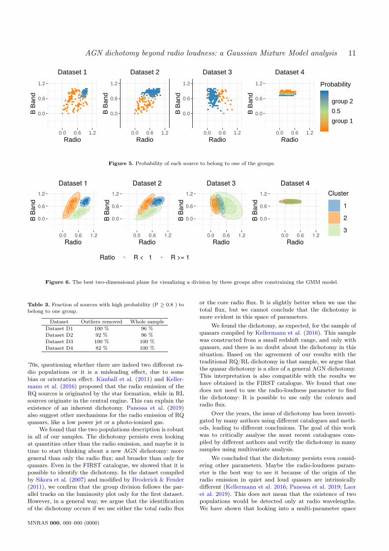
As a final test, we computed the GMM constraining thenumber of groups to 3 to verify if the method could separatethe sources around probability 0.5 into a group on its own.This division of the sources with probability around 0.5 ina group off its own happens only for dataset 4: when welook to the plane radio versus optical, (Figure 6). Somethingdifferent occurs for datasets D1 and D2: a third group alsoappears, but it does not necessarily contain sources withprobability 0.5. In dataset D3, there was no source withless than 0.8 of the likelihood to belong to a given group(Table 3), and we only see an artificial transition zone. Thesituation is not straightforward for datasets D1 and D2. Themethod provided three distinct groups, but none of themcorrespond to the sources that have probability 0.5 on thedichotomy split.

6 CONCLUSION

The existence of a dichotomy in the radio extragalacticsources has been discussed since its definition in the late

MNRAS 000, 000–000 (0000)

AGN dichotomy beyond radio loudness: a Gaussian Mixture Model analysis 11

0.0

0.6

1.2

0.0 0.6 1.2Radio

B B

and

Dataset 1

0.0

0.6

1.2

0.0 0.6 1.2Radio

B B

and

Dataset 2

0.0

0.6

1.2

0.0 0.6 1.2Radio

B B

and

Dataset 3

0.0

0.6

1.2

0.0 0.6 1.2Radio

B B

and

Dataset 4

group 1

0.5

group 2

Probability

Figure 5. Probability of each source to belong to one of the groups.

0.0

0.6

1.2

0.0 0.6 1.2Radio

B Ba

nd

Dataset 1

0.0

0.6

1.2

0.0 0.6 1.2Radio

B Ba

nd

Dataset 2

0.0

0.6

1.2

0.0 0.6 1.2Radio

B Ba

ndDataset 3

0.0

0.6

1.2

0.0 0.6 1.2Radio

B Ba

nd

Dataset 4

Ratio R < 1 R >= 1

Cluster

1

2

3

Figure 6. The best two-dimensional plane for visualizing a division by three groups after constraining the GMM model.

Table 3. Fraction of sources with high probability (P ≥ 0.8 ) tobelong to one group.

Dataset Outliers removed Whole sampleDataset D1 100 % 96 %

Dataset D2 92 % 96 %

Dataset D3 100 % 100 %Dataset D4 82 % 100 %

’70s, questioning whether there are indeed two different ra-dio populations or it is a misleading effect, due to somebias or orientation effect. Kimball et al. (2011) and Keller-mann et al. (2016) proposed that the radio emission of theRQ sources is originated by the star formation, while in RLsources originate in the central engine. This can explain theexistence of an inherent dichotomy. Panessa et al. (2019)also suggest other mechanisms for the radio emission of RQquasars, like a low power jet or a photo-ionized gas.

We found that the two populations description is robustin all of our samples. The dichotomy persists even lookingat quantities other than the radio emission, and maybe it istime to start thinking about a new AGN dichotomy: moregeneral than only the radio flux; and broader than only forquasars. Even in the FIRST catalogue, we showed that it ispossible to identify the dichotomy. In the dataset compiledby Sikora et al. (2007) and modified by Broderick & Fender(2011), we confirm that the group division follows the par-allel tracks on the luminosity plot only for the first dataset.However, in a general way, we argue that the identificationof the dichotomy occurs if we use either the total radio flux

or the core radio flux. It is slightly better when we use thetotal flux, but we cannot conclude that the dichotomy ismore evident in this space of parameters.

We found the dichotomy, as expected, for the sample ofquasars compiled by Kellermann et al. (2016). This samplewas constructed from a small redshift range, and only withquasars, and there is no doubt about the dichotomy in thissituation. Based on the agreement of our results with thetraditional RQ/RL dichotomy in that sample, we argue thatthe quasar dichotomy is a slice of a general AGN dichotomy.This interpretation is also compatible with the results wehave obtained in the FIRST catalogue. We found that onedoes not need to use the radio-loudness parameter to findthe dichotomy: It is possible to use only the colours andradio flux.

Over the years, the issue of dichotomy has been investi-gated by many authors using different catalogues and meth-ods, leading to different conclusions. The goal of this workwas to critically analyse the most recent catalogues com-piled by different authors and verify the dichotomy in manysamples using multivariate analysis.

We concluded that the dichotomy persists even consid-ering other parameters. Maybe the radio-loudness param-eter is the best way to see it because of the origin of theradio emission in quiet and loud quasars are intrinsicallydifferent (Kellermann et al. 2016; Panessa et al. 2019; Laoret al. 2019). This does not mean that the existence of twopopulations would be detected only at radio wavelengths.We have shown that looking into a multi-parameter space

MNRAS 000, 000–000 (0000)

12 Pedro P. B. Beaklini

can reveal a broad sense of dichotomy, expanding the evi-dence of two populations for all the AGNs. New data of theVLA Sky Survey (Lacy et al. 2020) can provide new infor-mation about the dichotomy slice at radio wavelength, anda future cross-match with catalogues at other wavelengthscould reveal even more hints about the nature of the differ-ence between the populations.

Using the GMM method, we were able to find the exis-tence of two groups in all the samples reliably. We interpretthese groups as two AGN populations that manifest them-selves as a dichotomy in the parameter space of luminosities,radio loudness R, central mass, colour, and even the radiooptical displacement.

We recall that the traditional RQ/RL dichotomy seemsto be a slice of the more general AGN dichotomy seen in thefull parameter space. This interpretation can explain whywe do not clearly see the division between RQ and RL in agiven sample.

In this work, we tried to identify as much as possiblea given group with the well-known traditional Radio Loudgroup. However, such correspondence is not necessarily ac-curate since it is possible to find a source with a low radioloudness value similar to a bright radio source due to otherparameters. Finally, further studies are needed to addresswhich is the best way to label both populations.

7 DATA AVAILABILITY

There is no new data analysed in this work. We have usedthe data published in the works presented in table 1.

8 ACKNOWLEDGEMENTS

We would like to acknowledge the anonymous referee forthe important comments that improve the work. The au-thors thank Dr. Rafael S. de Souza for the insightful sug-gestions during the preparation of this manuscript. PPBBacknowledges the FAPESP Thematic Project 2011/51676-9and Post-doc Project 2014/07460-0. MGBA acknowledgesthe FAPESP Thematic Project 2013/26258-4 and CNPqProject 150999/2018-6. MLLD acknowledges CAPES Fi-nance Code 001 and CNPq project 142294/2018-7.

References

Antonucci R., 1993, ARA&A, 31, 473Barret D., Cappi M., 2019, A&A, 628, A5Becker R. H., White R. L., Helfand D. J., 1995, ApJ, 450, 559Best P. N., Heckman T. M., 2012, MNRAS, 421, 1569Bian W., Zhao Y., 2002, A&A, 395, 465Biernacki C., Celeux G., Govaert G., 2000, IEEE Transactions on

Pattern Analysis and Machine Intelligence, 22, 719Blandford R. D., Königl A., 1979, ApJ, 232, 34Bonchi A., La Franca F., Melini G., Bongiorno A., Fiore F., 2013,

MNRAS, 429, 1970Brenneman L., 2013, Measuring the Angular Momentum of Su-

permassive Black Holes, doi:10.1007/978-1-4614-7771-6.Broderick J. W., Fender R. P., 2011, MNRAS, 417, 184Cao X., Rawlings S., 2004, MNRAS, 349, 1419Chiu H.-Y., 1964, Physics Today, 17, 21

Cirasuolo M., Magliocchetti M., Celotti A., Danese L., 2003a,MNRAS, 341, 993

Cirasuolo M., Celotti A., Magliocchetti M., Danese L., 2003b,MNRAS, 346, 447

Condon J. J., Odell S. L., Puschell J. J., Stein W. A., 1980, Na-ture, 283, 357

Daly R. A., Stout D. A., Mysliwiec J. N., 2018, ApJ, 863, 117Dempster A. P., Laird N. M., Rubin D. B., 1977, Journal of the

Royal Statistical Society. Series B (Methodological), 39, 1Efron B., Petrosian V., 1992, ApJ, 399, 345Eracleous M., Halpern J. P., 1994, ApJS, 90, 1Eracleous M., Halpern J. P., 2003, ApJ, 599, 886Falcke H., Sherwood W., Patnaik A. R., 1996a, ApJ, 471, 106Falcke H., Patnaik A. R., Sherwood W., 1996b, ApJ, 473, L13Falcke H., Körding E., Markoff S., 2004, A&A, 414, 895Fanaroff B. L., Riley J. M., 1974, MNRAS, 167, 31PFanti C., Fanti R., Lari C., Padrielli L., van der Laan H., de Ruiter

H., 1977, A&A, 61, 487Fraley C., Raftery A. E., 2002, Journal of the American Statistical

Association, 97, 611Fuentes C., Casella G., 2009, SORT, 33 2, 115Gopal V., Fuentes C., Casella G., 2012, Journal of Statistical

Software, 47, 1Hastie T., Tibshirani R., Friedman J., 2001, The Elements of Sta-

tistical Learning. Springer Series in Statistics, Springer NewYork Inc., New York, NY, USA

Ho L. C., 2002, ApJ, 564, 120Ho L. C., 2008, ARA&A, 46, 475Ho L. C., Peng C. Y., 2001, ApJ, 555, 650Holt S. S., Neff S. G., Urry C. M., 1992, Science, 257, 1779Johnson R. A., Bhattacharyya G. K., 2006, Statistics: Principles

and methods, 6. ed edn. Wiley series in probability and statis-tics, John Wiley & Sons, Hoboken, NJ

Katgert P., Katgert-Merkelijn J. K., Le Poole R. S., van der LaanH., 1973, A&A, 23, 171

Kellermann K. I., Pauliny-Toth I. I. K., 1966, Nature, 212, 781Kellermann K. I., Sramek R., Schmidt M., Shaffer D. B., Green

R., 1989, AJ, 98, 1195Kellermann K. I., Condon J. J., Kimball A. E., Perley R. A.,

Ivezić Ž., 2016, ApJ, 831, 168Kharb P., Shastri P., 2004, A&A, 425, 825Kimball A. E., Kellermann K. I., Condon J. J., Ivezić Ž., Perley

R. A., 2011, ApJ, 739, L29Körding E. G., Jester S., Fender R., 2008, MNRAS, 383, 277Lacy M., Laurent-Muehleisen S. A., Ridgway S. E., Becker R. H.,

White R. L., 2001, ApJ, 551, L17Lacy M., et al., 2020, PASP, 132, 035001Laor A., Baldi R. D., Behar E., 2019, MNRAS, 482, 5513Mahony E. K., Croom S. M., Boyle B. J., Edge A. C., Mauch T.,

Sadler E. M., 2010, MNRAS, 401, 1151Mahony E. K., Sadler E. M., Croom S. M., Ekers R. D., Feain

I. J., Murphy T., 2012, ApJ, 754, 12McLachlan G., Krishnan T., 2008, The EM algorithm

and extensions, 2. ed edn. Wiley series in prob-ability and statistics, Wiley, Hoboken, NJ, http://gso.gbv.de/DB=2.1/CMD?ACT=SRCHA&SRT=YOP&IKT=1016&TRM=ppn+52983362X&sourceid=fbw_bibsonomy

McLachlan G. J., Peel D., 2000, Finite mixture models. Wileyseries in probability and statistics, J. Wiley & Sons, New York,http://opac.inria.fr/record=b1097397

Mengersen K., Robert C., Titterington M., 2011, Mixtures: Es-timation and Applications. Wiley Series in Probability andStatistics, Wiley, https://books.google.com.br/books?id=9JJU_V49MmwC

Merloni A., Heinz S., di Matteo T., 2003, MNRAS, 345, 1057Moderski R., Sikora M., Lasota J. P., 1998, MNRAS, 301, 142Murdoch H. S., Crawford D. F., 1977, MNRAS, 180, 41P

MNRAS 000, 000–000 (0000)

AGN dichotomy beyond radio loudness: a Gaussian Mixture Model analysis 13

Murphy K. P., 2012, Machine Learning: A Probabilistic Perspec-tive. The MIT Press

Panessa F., Baldi R. D., Laor A., Padovani P., Behar E., McHardyI., 2019, Nature Astronomy, 3, 387

Peterson B. M., 1997, An Introduction to Active Galactic NucleiR Core Team 2016, R: A Language and Environment for Sta-

tistical Computing. R Foundation for Statistical Computing,Vienna, Austria, https://www.R-project.org/

Rafter S. E., Crenshaw D. M., Wiita P. J., 2009, AJ, 137, 42Raftery A. E., 1995, Sociological Methodology, 25, 111Rees M. J., 1966, Nature, 211, 468Retana-Montenegro E., Röttgering H. J. A., 2017, A&A, 600, A97Scheuer P. A. G., Readhead A. C. S., 1979, Nature, 277, 182Schmidt M., Green R. F., 1983, ApJ, 269, 352Schneider D. P., et al., 2010, AJ, 139, 2360Schoenmakers A. P., de Bruyn A. G., Röttgering H. J. A., van

der Laan H., Kaiser C. R., 2000, MNRAS, 315, 371Shapiro I. I., Weinreb S., 1966, ApJ, 143, 598Sikora M., Stawarz Ł., Lasota J.-P., 2007, ApJ, 658, 815Singal J., Petrosian V., Lawrence A., Stawarz Ł., 2011, ApJ, 743,

104Singal J., Petrosian V., Stawarz Ł., Lawrence A., 2013, ApJ, 764,

43Smith M. G., Wright A. E., 1980, MNRAS, 191, 871Sramek R. A., Weedman D. W., 1980, ApJ, 238, 435Strittmatter P. A., Hill P., Pauliny-Toth I. I. K., Steppe H., Witzel

A., 1980, A&A, 88, L12Sulentic J. W., Marziani P., Dultzin-Hacyan D., 2000, ARA&A,

38, 521Sulentic J. W., Martínez-Carballo M. A., Marziani P., del Olmo

A., Stirpe G. M., Zamfir S., Plauchu-Frayn I., 2015, MNRAS,450, 1916

Ucci G., Ferrara A., Pallottini A., Gallerani S., 2018, MNRAS,477, 1484

Unal C., Loeb A., 2020, arXiv e-prints, p. arXiv:2002.11778Urry C. M., Padovani P., 1995, PASP, 107, 803Van Gorkom K. J., Wardle J. F. C., Rauch A. P., Gobeille D. B.,

2015, MNRAS, 450, 4240Wals M., Boyle B. J., Croom S. M., Miller L., Smith R., Shanks

T., Outram P., 2005, MNRAS, 360, 453White R. L., Becker R. H., Helfand D. J., Gregg M. D., 1997,

ApJ, 475, 479White R. L., et al., 2000, ApJS, 126, 133Woo J.-H., Urry C. M., 2002, ApJ, 579, 530de Souza R. S., et al., 2017, MNRAS, 472, 2808

MNRAS 000, 000–000 (0000)