Embed Size (px)
Citation preview
Department of Computer ScienceFaculty of Mathematics, Physics and Informatics
Comenius University, Bratislava
Agrawal’s Conjectureand Carmichael Numbers
(master’s thesis)
Tomáš Váňa
advisor:RNDr. Martin Mačaj, PhD. Bratislava, 2009

iii
I hereby declare that I wrote this master’s thesismyself with the help of the referenced literature,under the supervision of my advisor.
. . . . . . . . . . . . . . . . . . . . . . . . . . . . . . . . .

iv
Contents
1 Introduction 1
2 Primality testing 3
3 Carmichael numbers 11
4 Sophie-Germain primes 17
5 Lenstra-Pomerance heuristic 21
6 Search for counterexample 29
7 Fibonacci & matrix approach 33
8 Experimental data 49
9 Conclusion 55
Bibliography 57
Abstract 59
v

vi CONTENTS
Chapter 1
Introduction
The main interest and high level view of our story will be the prime numbersand how to recognize them apart from composites. This problem wasformulated by ancient mathematicians long before there were any notions liketime complexity or any practical need of testing large numbers for primalitylike we know it nowadays in cryptography. Like many problems in numbertheory, it remained unsolved for hundreds of years, until quite recently therewere some significant breakthroughs in this area.
First revolutionary invention were the probabilistic primality tests, whichhave some very small probability of giving an incorrect answer. On theother side, they are very fast, not only polynomial with respect to the lengthof the input, but also practically usable. Of course for mathematicians,any probability that the result might be wrong, however small, still makesthe solution unsatisfactory. In this text we will speak more about anotherbreakthrough, which was to fill the gap of uncertainty and to construct analgorithm without this small error probability flaw. We will start with abrief evolvement overview of the primality testing algorithms and look at thedeterministic test discovered by Indian mathematicians Manindra Agrawal,Neeraj Kayal and Nitin Saxena in august 2002.
Before the test was discovered, the authors formulated the followingconjecture which they hoped would bring a deterministic primality test.
Conjecture 1.1 (Agrawal) Let n,r be relatively prime integers, for which
(x− 1)n ≡ xn − 1 (mod xr − 1, n)
holds. Then either n is prime, or n2 ≡ 1 (mod r) has to hold.
1
2 CHAPTER 1. INTRODUCTION
They have not been successful in proving this conjecture and even nowwe do not know whether it is true or not. Finally the test they have foundis based on some other ideas, however, if true, the conjecture would stillprovide a significant speed up of the test. In this text we will present ourresults related to the conjecture and try to give some new ideas that can helpwith the research.
We will first demonstrate some reasons for the formulation of theconjecture, starting with a question about the choice of parameters madein the test and when can this choice lead to difficulties. To deal with thisproblem, we will try a combinatoric approach of using binomial theoremand some familiar tricks for manipulating the sums, as an alternative to thealgebraic approach using Chinese remainder theorem. In both ways we willprove an interesting result showing that for some choices of parameters theCarmichael numbers are making the same troubles as in other tests. In nextchapter we will present another choice of parameters where Sophie-Germainprime conjecture comes into play and implies that there is an infinite set ofcomposite numbers satisfying the congruence in the AKS test.
We will then analyze some special cases of the conjecture and develop analgorithm for calculating parameters that can be used to test its validity in afaster way. Along with this algorithm we will provide an alternative proof forthe theorem proposed by Lenstra and Pomerance which suggest that thereis a way to find the counterexample to the conjecture.
As a result of further research of the related theory we will demonstratehow to use matrices instead of polynomials to find a connection between thecongruence used in AKS test and some special linear recurrent sequences. Wewill develop a generic way to construct those sequences and demonstrate inthe special case that it leads to the well-known Fibonacci sequence. This willgive us an alternative way of proving the result of authors of the AKS testwhere they have shown the numbers satisfying the test with some specialparameters actually have to be Fibonacci pseudoprimes. In our text wewill additionally show that in some cases we are also dealing with Fermatpseudoprimes to particular bases.
We will conclude our story with a set of experimental results which wehave collected using the theoretical results from the previous text and someavailable records of numbers with special properties. We hope this textpresents our ideas and objectives clearly and will be a pleasant tour for thereader, possibly inspiring him to a further study of the presented topics orhelping with the research.
Chapter 2
Primality testing
To give the reader a better insight into the motivation of our story, we willmention in this chapter some of the ways to test whether a given integer is aprime number. We will give a brief overview of these methods, but to get adeeper view we strongly recommend the texts [5] and [6], which also containthe original references for all the theorems in this chapter.
First obvious way to find out whether a number is prime, is to follow thedefinition and simply search the range of possible divisors. This approach iscalled trial division and it comes as no surprise that it is too slow to use forlarge inputs.
What seems to be necessary to speed up the test, is another characteri-zation of the prime numbers, i.e. some condition equivalent to the primalitywhich is faster to verify. There are such conditions which may seem goodcandidates at the first sight, the following one is a good example.
Theorem 2.1 (Wilson’s theorem) Let p be an integer, p > 1. Then p isprime if and only if (p− 1)! ≡ −1 (mod p).
However, a closer look tells us that we actually do not know how tocalculate the factorial in the congruence in any faster way than the usualiterative multiplication, which means that by using the Wilson’s theoremas a primality test we get an even slower algorithm than the trial division.Actually, mathematicians were not very successful in searching for a suitableequivalent condition, but there was another breakthrough idea.
If we consider a necessary condition for primality which is not sufficientin general, we may get much better results in the sense of the speed. Of
3
4 CHAPTER 2. PRIMALITY TESTING
course this also means that there will be composite numbers passing ourtest and we have to somehow distinguish them. There is a whole familybased on a simple criterion called Fermat’s little theorem, we will showsome of them in this overview. Apart from the probabilistic tests basedon Fermat’s little theorem, there are some other methods of primalitytesting, most notably the Elliptic curve primality proving (ECPP) and theAdleman-Pomerance-Rumely (APR) test, improved by Cohen and Lenstrato get the time complexity (log n)O(log log logn). These tests are using quitecomplex results and notions from the number theory, which makes them lessintelligible for the general audience.
Theorem 2.2 (Fermat’s little theorem) Let p be a prime number. Forany integer a we have ap ≡ a (mod p). Moreover, if a is coprime to p, wehave ap−1 ≡ 1 (mod p).
There is a fast way to calculate the modular powers which uses thebinary representation of the exponent p, which means we have gained speed.Another advantage of this condition is the parameter a. If p is prime, thetheorem has to hold for any choice of a, and by choosing more of them we canincrease the probability that the result we get is really true. This parameteris usually called a base and a composite number that passes the Fermat’stest for some base a is called base-a pseudoprime. The natural question thatarises is whether we can choose a set of bases such that no composite numberwill pass the test for all of them. If there would be such a set which is smallenough, we could turn this into a quickly verifiable sufficient condition aswell. Unfortunately, there is no such set, because there are composites whichpass the test for any base.
Definition 2.1 Let n be a composite integer. If for any integer a it is truethat an ≡ a (mod n), we call the number n a Carmichael number.
It was proved that there are infinitely many Carmichael numbers and thefollowing criterion was found to recognize them.
Theorem 2.3 (Korselt’s criterion) Let n be an odd integer. Then n is aCarmichael number if and only if
a) It is square-free, i.e. not divisible by any square of a prime number.
b) For each of its prime divisors p it is true that p− 1 | n− 1.
5
Although the Korselt’s criterion characterizes the Carmichael numbersin an alternative way which is very useful for theoretical manipulations,without knowing the prime factorization (which we certainly do not knowwhen testing for primality) it does not help too much to recognize them. Onthe other side, when we are lucky enough to pick a composite number whichis not Carmichael, we have a very high chance of identifying it.
Lemma 2.1 Let n be an integer. If there is a number a, coprime to n, forwhich the congruence an−1 ≡ 1 (mod n) does not hold, then this congruenceholds for at most half of the numbers in set {1, . . . , n} coprime to n.
The real breakthrough idea is to use this fact and pick base a randomlymultiple times. In each step we have roughly 50% probability of finding outthat the number is composite (if it is not prime or Carmichael). Repeatingsuch a test decreases the probability of wrong decision exponentially and wecan bound it with such a low constant that for practical purposes we can bealmost sure that the result is correct.
Unfortunately we cannot ignore Carmichael numbers because there aretoo many of them. What can be done though, is to formulate the necessarycondition in a different way.
Theorem 2.4 Let p be a prime number, p = 2st, where t is odd. Then forany a coprime to p we have either at ≡ 1 (mod p) or a2it ≡ −1 (mod p) forsome i ∈ {0, . . . , s− 1}.
Once again we can construct a primality test based on this condition.The idea itself was first discovered by Artjuhov and later independently bySelfridge. We call the composite numbers passing the test base-a strongpseudoprimes and there is a good reason for calling them strong, becausethere are no numbers analogous to the Carmichael numbers in this case. Infact, even the probability of getting false positives is lower in this case.
Theorem 2.5 Let n > 9 be an odd integer. If S(n) is the set of all bases0 ≤ a < n for which n is a strong pseudoprime, then |S(n)| ≤ 1
4ϕ(n), where
ϕ(n) is Euler’s totient function.
Theorem 2.6 Let k ≥ 3 and T ≥ 1 be integers. Algorithm which generatesa prime number by testing validity of the condition 2.4 for a random numbern ∈ (2k−1, 2k) and a random number a ∈ 〈2, n− 2〉, doing so T times, has aprobability of producing composite number less than 4−T .
6 CHAPTER 2. PRIMALITY TESTING
These two theorems, proved by Monier and Rabin, provide first variationof the so-called Rabin-Miller test, in this case a probabilistic one whichcan test or generate prime numbers based on the criterion from theorem2.4. Another variation, discovered by Miller (which is the reason why heappears in the name of the algorithm) is a deterministic version based on theExtended Riemann hypothesis and the following result.
Theorem 2.7 If the Extended Riemann hypothesis is true, then the smallestwitness of an odd composite number n is less than 2 ln2 n.
Witness is a name for the base which will not make the number a strongpseudoprime, i.e. when the test is performed with this number as a parametera, it will find out that the number is composite. It is therefore enough toperform the test for all a’s from the set {1, . . . , 2 ln2 n} and we are sure (ifwe believe that the Extended Riemann hypothesis is true), that the result iscorrect.
Although both of these approaches have their flaws (the first somenon-zero error probability and the second dependency on a conjecture),the variation of this test is widely used for commercial purposes to testand generate prime numbers. The main reason for that is the speed andsimplicity. There are many other approaches to probabilistic primalitytesting, e.g. Solovay-Strassen test dealing with quadratic residues etc. Inone of the following chapters we will deal with the Fibonacci test andpseudoprimes, therefore we add it here to our overview.
Theorem 2.8 Let us denote by fn the n-th Fibonacci number (starting withf0 = 0, f1 = 1). If n is a prime number, then the following holds
a) fn−1 ≡ 0 (mod n) for n ≡ ±1 (mod 5)
b) fn+1 ≡ 0 (mod n) for n ≡ ±2 (mod 5)
Analogously to the previous tests, we call numbers that satisfy this conditionin spite of being composite the Fibonacci pseudoprimes.
Next important step in the family of simple algorithms based on variationsand generalizations of Fermat’s little therorem was an algorithm found in theyear 2002 by Indian mathematicians Agrawal, Kayal and Saxena and is calledby their names, AKS test. The very basic idea of the algorithm is surprisinglysimple, as the next lemma shows.
7
Lemma 2.2 Let n be an integer, then for all integers a, for which (a, n) = 1,the following congruence
(x+ a)n ≡ xn + a (mod n) (2.1)
holds iff n is prime.
Proof Using the binomial theorem, we can expand the left side of thecongruence to a well-known sum
(x+ a)n =n∑k=0
(n
k
)xkan−k
We are especially interested in the first and the last member of the expansion,as they are the same degrees as we have on the right side of our congruence.Therefore let us write
(x+ a)n = xn +∑
0<k<n
(n
k
)xkan−k + an
First, let us assume that n is prime. Then by Fermat’s little theorem we havean ≡ a (mod n), and all we have to show is that the sum in the middle iscongruent to zero. This is done quite easily – we just have to realize that thebinomial coefficient
(nk
)can be written as nk
k!, where nk = n · (n− 1) · · · (n−
k + 1). The numerator of this fraction is obviously divisible by n. However,because n is prime, there is no other number which would divide n and beless than n (except for 1 of course, but this is irrelevant). Therefore, there isnothing in the denominator that would cancel out the prime n and the wholenumber is divisible by n. This means all the terms of the sum are divisibleby n and the sum itself is congruent to zero, so we are done.
Now let us assume that n is not a prime number and let p be a primedivisor of n. We will take a look just at the coefficient(
n
p
)=n · · · (n− p+ 1)
p · · · 1
If pα is the highest power of p that divides n, then the numerator is divisibleby pα (only the factor n is divisible by p) and the denominator is divisible bythe first power of p (the factor p). Therefore, the whole fraction is divisible
8 CHAPTER 2. PRIMALITY TESTING
only by pα−1 and cannot be divisible by n, also the coefficient an−p whichgets multiplied by it will not help, as (a, p) = 1. �
The previous lemma gives us an equivalent condition of primality. Wehave seen that there are troubles with such conditions and this is not anexception – testing it requires to calculate a polynomial of enormous size,which makes it even slower and more memory consuming than the trialdivision test.
To make it more than just another curiosity like Wilson’s theorem, wetake the congruence and reduce it modulo some polynomial of a small degree,namely xr − 1, where r is of polylogarithmic size. Because we have shownthat the congruence holds for primes, reducing it further cannot break thisproperty and it is still true that
(x+ a)n ≡ xn + a (mod xr − 1, n) (2.2)
for prime n. For simplicity, we will in the following text refer to thiscongruence as T (a, n, r). This new congruence can hold for some compositen as well – taking the simplest example of r = 1, we have reduced our testto the Fermat’s test.
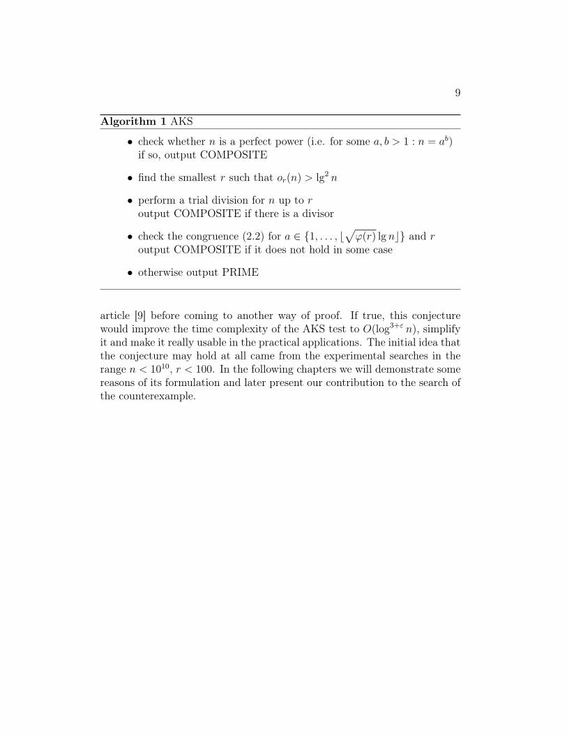
Our goal is therefore to choose r and a in such a way that we gain speed,but do not lose the equivalence with primality condition. Authors of thetest have shown that there is indeed a way to choose those parameters thatmakes it fast and still keeps the other direction of the equivalence holding,at least to some extent. We will state their algorithm here, the proof andtime-complexity analysis can be found in the original article [1].
After the AKS algorithm was discovered, there were many improvementsmade by other mathematicians and some of them have shifted the timecomplexity from the original O(log7.5+ε n) to O(log6+ε n). There aresome modifications of the proof that only guarantee the time complexityO(log12+ε n), but make the arguments in a more elementary way which isintelligible with basic knowledge of algebra and number theory. However,even these improvements were not enough to make the test practical enoughand it still remains just a theoretical result at this time (for practicalpurposes, probabilistic algorithms are used).
An important questions that remains open will be the main topic of ourwhole story. We have already mentioned the Agrawal’s conjecture in theintroduction, this is the direction that authors have been trying to go in the
9
Algorithm 1 AKS
• check whether n is a perfect power (i.e. for some a, b > 1 : n = ab)if so, output COMPOSITE
• find the smallest r such that or(n) > lg2 n
• perform a trial division for n up to routput COMPOSITE if there is a divisor
• check the congruence (2.2) for a ∈ {1, . . . , b√ϕ(r) lg nc} and r
output COMPOSITE if it does not hold in some case
• otherwise output PRIME
article [9] before coming to another way of proof. If true, this conjecturewould improve the time complexity of the AKS test to O(log3+ε n), simplifyit and make it really usable in the practical applications. The initial idea thatthe conjecture may hold at all came from the experimental searches in therange n < 1010, r < 100. In the following chapters we will demonstrate somereasons of its formulation and later present our contribution to the search ofthe counterexample.

10 CHAPTER 2. PRIMALITY TESTING
Chapter 3
Carmichael numbers
In the previous chapter we have said that putting r = 1 in the congruence(2.2) reduces testing of the congruence to the Fermat’s test and therefore hasall its flaws in that case. Authors have shown that choosing r in such a waythat or(n) > lg2 n seems to be enough to eliminate any flaws when combinedwith a suitable set of a’s. The question we want to ask in this chapter iswhether there are some choices of r which are so bad that there is no set ofa’s that would help to distinguish composites from primes, exactly as it waswith the Carmichael numbers in case of the Fermat’s test.
In the next lemma we will show that AKS test is not worse than Fermat’stest for any choice of r. What we mean by that is that if it fails for somenumber n and all choices of a’s, then this number n has to be Carmichael.
Lemma 3.1 Let n and r be some fixed integers and suppose T (a, n, r) holdsfor any choice of a. Then an ≡ a (mod n) for all integers a.
Substituting x = 1 into T (a, n, r) we have directly
(1 + a)n ≡ 1 + a (mod n)
However, this is just a shift of the congruence we want to prove and we canchange a for a− 1, therefore we are done. �
The next step to answer our question is to ask whether there are choicesof r which make the testing of the congruence T (a, n, r) fail for Carmichaelnumbers and all choices of a. We will start with the combinatoric approach,in order to dig deeper into the structure of the polynomial powers in our
11
12 CHAPTER 3. CARMICHAEL NUMBERS
congruence, and later we will show the same with a standard algebraicapproach, just to see the difference between the methods.
Theorem 3.1 Let n = p1 · · · pk be a Carmichael number and r | (p1−1, p2−1, . . . , pk − 1). Then T (a, n, r) holds for any integer a.
We will need two lemmas before coming to the proof.
Lemma 3.2 Let p = rs + 1 be a prime number and let g be a generator ofthe cyclic group Z∗p . Then for any integer k it is true that
r−1∑i=0
gisk ≡{r (mod p) when r | k0 (mod p) when r - k
Proof It is easy to see that the condition r | k is equivalent to p − 1 | sk.Because g is the generator of the cyclic group Z∗p , this is further equivalentto the congruence gsk ≡ 1 (mod p). If it holds, every summand is 1 modulop, so it is not hard to see that the sum of r such numbers is exactly r. Letus have a look at the sum in the second case and let us denote its value byS. We have
gsk · S ≡r−1∑i=0
g(i+1)sk = S − g0 + grsk (mod p)
Because rs = p− 1, we have grsk ≡ g0 = 1 (mod p), and therefore
gsk · S ≡ S (mod p)
Another manipulation gives us
S(gsk − 1) ≡ 0 (mod p)
and from the assumption we know that the second factor is not zero, whichmeans p has to divide the first one, i.e. S ≡ 0 (mod p), which is the fact wewanted to prove. �
Lemma 3.3 Let n = rq + 1 be a Carmichael number and let p = rs + 1 bea prime divisor of n. Then for any integers a and t we have
∑0≤j≤n
j≡t (mod r)
(n
j
)aj ≡
1 (mod p) when t ≡ 0 (mod r)a (mod p) when t ≡ 1 (mod r)0 (mod p) when t 6≡ 0, 1 (mod r)
13
Proof Let g be a generator of the cyclic group Z∗p . Let us have a look atthe following sum
S1 =r−1∑i=0
(gsi + a)n · gsi(t−1)
According to the binomial theorem we get
S1 =r−1∑i=0
gsi(t−1)
n∑j=0
(n
j
)aj · gsi(n−j) =
r−1∑i=0
n∑j=0
(n
j
)aj · gsi(n−j+t−1)
Changing the order of the summation we further have
S1 =n∑j=0
r−1∑i=0
(n
j
)aj · gsi(n−j+t−1) =
n∑j=0
(n
j
)aj
r−1∑i=0
gsi(n−j+t−1)
Now we are going to use the lemma 3.2 to calculate the inner sum. Goingfrom there this sum is always zero modulo p, except for the case when r |n − j + t − 1, in other words when j ≡ t (mod r). In this case the value ofthe sum, according to the lemma 3.2, is exactly r, which means we have
S1 ≡ r ·∑
0≤j≤nj≡t (mod r)
(n
j
)aj (mod p)
Now let us start with the original sum S1 and follow a different path ofmanipulations. We will use the fact that n is a Carmichael number, whichmeans that (gsi + a)n ≡ gsi + a (mod n), and because p | n this also impliesthat (gsi + a)n ≡ gsi + a (mod p). Therefore
S1 ≡r−1∑i=0
(gsi + a) · gsi(t−1) (mod p)
and
S1 ≡r−1∑i=0
gsit + a ·r−1∑i=0
gsi(t−1) (mod p)
Now let us use the lemma 3.2 once again to calculate the value of both sums.The first one is always zero, except for the case when r | t, having value r inthat case. The second sum is always zero, except for the case when r | t− 1,
14 CHAPTER 3. CARMICHAEL NUMBERS
or t ≡ 1 (mod r), having value r in that case. Summing up what we havelearned so far we have
S1 ≡
r (mod p) when t ≡ 0 (mod r)ra (mod p) when t ≡ 1 (mod r)0 (mod p) when t 6≡ 0, 1 (mod r)
Now let us callS2 =
∑0≤j≤n
j≡t (mod r)
(n
j
)aj
We have shown that S1 ≡ r · S2 (mod p) holds, which means we have
r · S2 ≡
r (mod p) when t ≡ 0 (mod r)ra (mod p) when t ≡ 1 (mod r)0 (mod p) when t 6≡ 0, 1 (mod r)
The last step is to cancel out the number r in all the congruences (asp = rs+ 1, the numbers p and r have to be relatively prime). This gives usthe relationship we wanted to prove. �
Now we are ready to prove the theorem 3.1. Apart from the fact that nis a product of distinct prime numbers, the Korselt’s criterion is telling usthat for all of these prime numbers it is true that pi− 1 | n− 1. Because r isa common divisor of all terms pi − 1, it has to be true that r | n− 1 as well.Let us therefore (for a suitable integer q) write n = rq+1. By expanding theleft side of the congruence we are proving according to the binomial theoremwe get
n∑i=0
(n
i
)aixn−i ≡ xn + a (mod xr − 1, n)
Now, realizing that xr ≡ 1 (mod xr − 1), we see that xi ≡ xi mod r
(mod xr − 1) for all non-negative exponents i. Let us denote the sum on theleft side of the congruence by S0 and using this fact rewrite it in the followingway :
S0 ≡r−1∑z=0
xz · ∑0≤j≤n
j≡n−z (mod r)
(n
j
)aj
(mod xr − 1, n)
15
Let us now consider any prime number pi, for which according to theassumption r | pi−1, so there is a suitable si so that we can write pi = rsi+1.Using the lemma 3.3 we get that
∑0≤j≤n
j≡n−z (mod r)
(n
j
)aj ≡
1 (mod pi) when n− z ≡ 0 (mod r)a (mod pi) when n− z ≡ 1 (mod r)0 (mod pi) when n− z 6≡ 0, 1 (mod r)
Using the fact that n ≡ 1 (mod r) we can easily rewrite that to the form
∑0≤j≤n
j≡n−z (mod r)
(n
j
)aj ≡
1 (mod pi) when z ≡ 1 (mod r)a (mod pi) when z ≡ 0 (mod r)0 (mod pi) when z 6≡ 0, 1 (mod r)
Additionally, as these congruences hold modulo any prime divisor pi of thenumber n, they have to hold modulo n as well, namely because n is a productof these distinct primes. This gives us
∑0≤j≤n
j≡n−z (mod r)
(n
j
)aj ≡
1 (mod n) when z ≡ 1 (mod r)a (mod n) when z ≡ 0 (mod r)0 (mod n) when z 6≡ 0, 1 (mod r)
Using this relationship we can easily calculate the value of the sum S0, wehave S0 ≡ a+x (mod xr−1, n). To conclude the proof, it is enough to realizethat it is true that xn ≡ x (mod xr − 1), as n ≡ 1 (mod r). Therefore wealso have
S0 ≡ a+ xn (mod xr − 1, n)
which is already the congruence we wanted to prove in the first place. �
In addition to the combinatoric proof that we have provided we will nowprove the theorem 3.1 in an alternative way, using the Chinese remaindertheorem for polynomials. Once again we will start from the fact that r | pi−1for any prime number pi and we will show that if we look at the congruenceT (a, n, r) modulo pi, it is true. Knowing that n is a product of distinctprimes this is enough to show that T (a, n, r) holds also in the original form,i.e. modulo n.
As a first step, we realize that from r | pi−1 we know that xr−1 | xpi−1−1.Namely, for a suitable integer s it has to be true that pi = rs+1, which means
16 CHAPTER 3. CARMICHAEL NUMBERS
xpi−1− 1 = xrs− 1 = (xr − 1)(x(s−1)r + x(s−2)r + . . .+ 1). Moreover, we havexpi−1−1 | xpi−x and we know that Zpi
is the splitting field of the polynomialxpi − x. This is implied by the fact that according to the little Fermat’stheorem, each member of this field is a root of the polynomial xpi − x andtherefore we can write this polynomial over this field as a product of factorsxpi−x ≡ x·(x−1) · · · (x−pi+1) (mod pi). Because the polynomial xr−1 is itsdivisor, there has to be a way of writing it analogically as a product of some ofthese factors (it would be r of them obviously), i.e. xr−1 ≡ (x−a1) · · · (x−ar)(mod pi), where a1, . . . , ar are distinct members of Z∗pi
. Now having the factthat all the polynomials x − aj are relatively prime we can use the Chineseremainder theorem to simplify our dealing with the congruence T (a, n, r).If we are lucky enough to show that for all j ∈ {1, . . . , r} it is true that(x+ a)n ≡ xn + a (mod x− aj, pi), then knowing that xr − 1 is a product ofthese relatively prime polynomials and using the Chinese remainder theoremwe get (x− 1)n ≡ xn − 1 (mod xr − 1, pi) as well. This would be, accordingto what has been said so far, enough to show that T (a, n, r) holds for any a.Fortunately, dealing with the congruence modulo x−aj is very simple, as wehave x ≡ aj (mod x − aj) which effectively means we can substitute aj forx, getting an equivalent congruence (aj − a)n ≡ anj − a (mod pi). From thefact that n is a Carmichael number we immediately have (aj − a)n ≡ anj − a(mod n), which is even more than we need, as pi | n. This means we aredone with the proof. �
We have demonstrated that there are choices of r such that testing thecongruence (2.2) can fail for all choices of a. This shows that there are somelimitations needed on the parameter r and although the condition or(n) >lg2 n might not be the tightest and there is still a place for improvements,there is a good reason to limit the r in this way (apart from the fact that itwas needed for the proof). More importantly, we have shown an interestingexample of two different points of view when dealing with the congruenceT (a, n, r). The algebraic approach turned out to be simpler, on the otherside by using the sum approach we have gained more insight into what ishappening when we are calculating powers of polynomials.
Chapter 4
Sophie-Germain primes
Another way of looking at the result from the previous chapter is that wehave shown in the case of r 6= 1 and r | n − 1, that there are infinitelymany composite numbers n for which T (a, n, r) holds. This correspondsto the Agrawal’s conjecture which is explicitly saying that this is ok whenr | n2 − 1. The question we want to ask now is whether it will help when werestrict the parameters in such a way that r - n − 1. Will there still be aninfinite set of composite numbers n satisfying the congruence ?
We will use simple choices of r = 4 and a = −1 to show that the situationseems to be similar when r | n + 1. First, let us start with an equivalentcharacterization of the congruence T (−1, n, 4) which will be easier to workwith.
Theorem 4.1 Let n be an integer. The congruence T (−1, n, 4) holds iff
a) 2n−1
2 · (−1)n−1
4 ≡ 1 (mod n) for n ≡ 1 (mod 4)
b) 2n−1
2 · (−1)n+1
4 ≡ 1 (mod n) for n ≡ 3 (mod 4)
Proof Let n = 4k + 3. It can be easily shown by induction that
22k · ((−22k+1 + (−1)k) + (22k+1 + (−1)k)x+
(−22k+1 − (−1)k)x2 + (22k+1 − (−1)k)x3)
is congruent to (x − 1)n in (x4 − 1, n). In the first step, taking k = 0, theexpression evaluates to x3 − 3x2 + 3x − 1, which is exactly (x − 1)3. In theinduction step we just multiply the expression by (x− 1)4 = 2(−2x3 + 3x2−
17
18 CHAPTER 4. SOPHIE-GERMAIN PRIMES
2x + 1) and we get the desired result for k + 1. To derive the equivalentproperty for T (−1, n, 4), we just have to compare the coefficients of desiredresult (x− 1)n, which should be the same as x3 − 1, to what we have in ourexpression. This gives us the following congruences :
22k(22k+1 − (−1)k) ≡ 1 (mod n)
22k(22k+1 + (−1)k) ≡ 0 (mod n)
When we subtract these we get directly the congruence 22k+1 · (−1)k+1 ≡ 1(mod n), which we wanted to prove in the first place. To get the otherdirection of equivalence, it is enough to realize that (n, 2) = 1 and bymultiplying the congruence by 2−1 and squaring both sides we can easilyderive both of the congruences equivalent to T (−1, n, 4), which concludesthe proof. In the case of n = 4k + 1, the proof is exactly the same, first weshow by induction that
22k−1 · ((−22k + (−1)k−1) + (22k − (−1)k−1)x+
(−22k − (−1)k−1)x2 + (22k + (−1)k−1)x3)
is in the same class of residues as (x− 1)n, then we compare the coefficientswith the desired result, in this case the polynomial x − 1. This way we getcongruences
22k−1(22k − (−1)k−1) ≡ 1 (mod n)
22k−1(22k + (−1)k−1) ≡ 0 (mod n)
Subtracting them gives us the congruence 22k · (−1)k ≡ 1 (mod n), which wewanted to prove (the other direction is done once again with squaring bothsides). �
For the concrete choices of parameters that we have made we no longerhave to deal with polynomial congruence, which gives us higher chancesof manipulating it successfully. One observation that is quite simple tomake, is that by squaring the congruences from 4.1 we immediately see thatfor a composite number n to satisfy them, it has to be a base-2 Fermat’spseudoprime. Therefore we were able to simply use the existing records ofpseudoprimes (up to 1015 collected William Galway – see [7]) to give us afeeling of how often the congruence T (−1, n, 4) holds. From the overall count
19
of 1801533 pseudoprimes in the range we searched through, there were 867198such that T (−1, n, 4) holds and n ≡ 1 (mod 4), and only 89913 were suchthat T (−1, n, 4) holds and n ≡ 3 (mod 4). The reason seems to be that thereis about 10 times more pseudoprimes with residue 1 than with residue 3 andfor both of them about a half satisfies the condition needed for T (−1, n, 4)to hold.
It all looks like for r = 4 there is a lot of examples we search for. The nextquestion we want to ask is whether this pattern holds also for large numbersand whether we can find an infinite sequence of numbers with T (−1, n, 4) andn ≡ 3 (mod 4). We will show that if the widely believed Sophie-Germainprimes conjecture is true, such a sequence can be easily constructed. Firstof all, let us introduce some necessary basics.
Definition 4.1 Let p be a prime number. We say that p is a Sophie-Germainprime if 2p+ 1 is a prime number as well.
The conjecture says that there are infinitely many Sophie-Germainprimes. Some very large examples were actually found (e.g. p = 8069496435 ·105072 − 1), but no proof was yet given. However, there are some heuristicarguments and estimations about the expected count of these numbers.The next theorem tells us about the connection between Sophie-Germanprimes and composite Mersenne numbers, which we will need for our proof.Mersenne numbers are numbers in form 2n − 1, especially interesting whenthe exponent n is prime.
Lemma 4.1 If Mn = 2n − 1 is prime, then n has to be a prime.
Proof If the n is composite, we can write n = ab (a, b > 1) and2n − 1 = 2ab − 1 = (2a − 1)(2a(b−1) + . . . + 1), therefore 2n − 1 is compositeas well. �
While p has to be prime for 2p − 1 to be prime as well, the converse isnot true and actually there are many such Mersenne numbers with primeexponents that are composite. It is not even known whether there areinfinitely many such composite or infinitely many such prime Mersennenumbers with prime exponents. We will now show the connection betweensuch numbers and Sophie-Germain primes (for more properties see [16]).
Theorem 4.2 Let p > 3 be a Sophie-Germain prime for which p ≡ 3(mod 4). Then the number Mp = 2p − 1 is composite.
20 CHAPTER 4. SOPHIE-GERMAIN PRIMES
Proof Let q = 2p + 1, we know that this number is prime. In addition,because p ≡ 3 (mod 4), we know that q ≡ 7 (mod 8). This implies(calculating the Legendre’s symbol, see e.g. [5]), that the number 2 is aquadratic residue (mod q), which by Euler’s criterion for quadratic residuesmeans that 2
q−12 = 2p ≡ 1 (mod q). Therefore, we have shown that
Mp = 2p−1 has a non-trivial factor of q = 2p+1, and has to be composite. �
Now we know that relying on a fact of having enough Sophie-Germainprimes (with the desired residue mod 4), there is enough composite Mersennenumbers with prime exponents as well. To finish our reasoning we will usethese numbers to construct the sequence of numbers which we were lookingfor.
Theorem 4.3 If p > 3 is a prime number and Mp = 2p − 1, thenT (−1,Mp, 4) holds.
Proof According to the theorem 4.1, we need to check the equivalentcongruence to know whether T (−1,Mp, 4) holds. The residue mod 4 is inthis case 3, so we have to prove that
2Mp−1
2 · (−1)Mp+1
4 ≡ 1 (mod Mp)
The exponent of −1 disappears immediately, as Mp+1
4= 2p−2 ≡ 0 (mod 2).
The congruence is equivalent to
22p−1−1 ≡ 1 (mod 2p − 1)
Now we will use the fact that p is prime and by Fermat’s theorem p | 2p−1−1.This means that the exponent is divisible by p and can be written in a formp · k for some k. This gives us the conclusion that 22p−1−1 = 2p·k = (2p)k ≡1k = 1 (mod 2p − 1) and the proof is done. �
From the theorem we now see the reason why we needed the Mersennenumbers to be composite – in the case of composite Mp we directly have anexample of a number for which the congruence holds, but r - n − 1, in factr | n + 1, and it seems very probable (based on the mentioned conjectures)that in this case we have infinitely many of them.
Chapter 5
Lenstra-Pomerance heuristic
If we combine the results from the previous two chapters, we see thatthere seem to be infinite sequences of composite numbers n satisfying thecongruence T (−1, n, r) in the case when r | n2− 1. This is a good reason forhaving this condition in the formulation of the Agrawal’s conjecture, but itis not clear whether it covers all the cases. In fact, the scientific communityin the area of the number theory researched this problem and formulatedseveral notes (see [12]) to the conjecture, most interesting being the followingtheorem, which provides a heuristic way to look for the counterexample forthe Agrawal’s conjecture.
Theorem 5.1 (Lenstra, Pomerance) Let p1, . . . , pk be distinct prime num-bers and let n = p1 · · · pk. If the following conditions hold
a) k ≡ 1 (mod 4) or k ≡ 3 (mod 4)
b) pi ≡ 3 (mod 80) for i ∈ {1, . . . , k}
c) pi − 1 | n− 1 for i ∈ {1, . . . , k}
d) pi + 1 | n+ 1 for i ∈ {1, . . . , k}
then the congruence T (−1, n, 5) holds, while n2 6≡ 1 (mod 5).
The authors in article [13] used arguments from analytical number theoryto show heuristic reasons for the existence of a number n satisfying thegiven conditions, and therefore being a counterexample for the Agrawal’sconjecture. They did not, however, give any concrete estimation of the size
21
22 CHAPTER 5. LENSTRA-POMERANCE HEURISTIC
of this number, nor did they give any way to find it. Before we will show thatthe theorem itself is true, we will prepare some auxiliary statements. Theproof we will give in this text differs slightly from the original proof and fromthe intermediate lemmas we will later derive a way to verify the congruenceT (−1, n, 5) in some special circumstances.
Definition 5.1 Let n be an arbitrary integer, for which (n, 5) = 1. Let usdenote by ρ(n) the smallest integer, for which the following is true
(x− 1)ρ(n)+1 ≡ x− 1 (mod x5 − 1, n) (5.1)
The number ρ(n) represents a multiplicative order of the element x− 1.First, let us show that the definition is correct and the number ρ(n) actuallyexists in all cases.
Lemma 5.1 Let n be an integer and let (n, 5) = 1. Then there is a numberr > 1, for which
(x− 1)r ≡ x− 1 (mod x5 − 1, n)
Proof We will show that if (n, 5) = 1 holds, we can in some limited waycancel out the term x− 1 from both sides of a congruence, if we have powersof this polynomial at the both sides of it. First of all, from the condition(n, 5) = 1 we know that there is an inverse element for the number 5 modulon. Let us call this inverse element a and consider the following polynomialsp(x) = 2ax4 + ax3 − ax− 2a and q(x) = x4 + x3 + x2 + x+ 1. We have
p(x) · (x− 1) ≡ −ax4 − ax3 − ax2 − ax+ 4a (mod x5 − 1, n)
what can be written as
p(x) · (x− 1) ≡ 5a− aq(x) (mod x5 − 1, n)
or by the definition of a
p(x) · (x− 1) ≡ 1− aq(x) (mod x5 − 1, n) (5.2)
The next congruence we will use is easy to verify as well
q(x) · (x− 1) ≡ 0 (mod x5 − 1, n) (5.3)
23
Putting them together we have
p(x) · (x− 1)2 = p(x) · (x− 1) · (x− 1) ≡(1− aq(x)) · (x− 1) = x− 1− aq(x) · (x− 1) ≡ (5.4)
x− 1− a · 0 = x− 1 (mod x5 − 1, n)
So we see that p(x) really can be used, in a limited way, as an inverse ofx− 1. Now we will come to the proof of the lemma itself. Because there areonly finitely many residue classes modulo x5 − 1, there has to be a pair ofexponents k 6= l for which
(x− 1)k ≡ (x− 1)l (mod x5 − 1, n) (5.5)
If k = 1 or l = 1, we are already done with the proof. Therefore let usassume, without the loss of generality that 1 < k < l. To conclude the proofit is enough to multiply the congruence (5.5) by the polynomial p(x)k−1 andrepeatedly use the relationship (5.4), which gives us
p(x)k−1 · (x− 1)k ≡ p(x)k−1 · (x− 1)l (mod x5 − 1, n)
x− 1 ≡ (x− 1)l−k+1 (mod x5 − 1, n)
and we have found the r = l − k + 1 we were looking for. �
Lemma 5.2 Let k, l be any integers and let ρ be the function we have definedabove. Then the congruence (x− 1)k ≡ (x− 1)l (mod x5− 1, n) holds if andonly if k ≡ l (mod ρ(n)) holds.
Proof The first implication is trivial, it results from the definition of ρ(n).In the other direction we can without loss of generality assume that k < l,because in the case k = l there is not much to prove. At the end of theprevious proof we have shown that having the congruence (5.5) we knowthat
x− 1 ≡ (x− 1)l−k+1 (mod x5 − 1, n) (5.6)
in the case k = 1 trivially and in the case k > 1 after canceling out theterms iteratively. On the other side we have defined the number ρ(n) as thesmallest integer with the property (5.1), telling us how often the remainderx− 1 will repeat itself in the sequence of powers. Because from this point on
24 CHAPTER 5. LENSTRA-POMERANCE HEURISTIC
the sequence is periodic, every other repetition has to happen exactly for thepowers that are further by the multiple of ρ(n). This means that ρ(n) | l− khas to hold, but that is only an equivalent way of stating the congruence thatwe are proving. �
Lemma 5.3 Let n be an integer for which (n, 5) = 1 and ρ the functiondefined above. If there exists λi(n), i ∈ {2, 3, 4} for which
(x− 1)λi(n) ≡ xi − 1 (mod x5 − 1, n)
then λ2(n)2 ≡ λ4(n) (mod ρ(n)), λ2(n)3 ≡ λ3(n) (mod ρ(n)), λ3(n)2 ≡λ4(n) (mod ρ(n)) and λ3(n)3 ≡ λ2(n) (mod ρ(n)). In fact, the existenceof λ2(n) or λ3(n) implies the existence of the remaining two.
Proof Let us take first the congruence
(x− 1)λ2(n) ≡ x2 − 1 (mod x5 − 1, n)
substituting x2 for x we get
(x2 − 1)λ2(n) ≡ x4 − 1 (mod x5 − 1, n)
comparing with the original congruence this gives us
(x− 1)λ2(n)2 ≡ x4 − 1 (mod x5 − 1, n)
from where we already have by the definition of the function ρ and lemma5.2 the first congruence we wanted to prove : λ2(n)2 ≡ λ4(n) (mod ρ(n)).The remaining congruences can be obtained in a similar way. �
Lemma 5.4 Let n be an integer and ρ the function defined above. If thereare suitable integers λi(n), i ∈ {2, 3, 4} such that
(x− 1)λi(n) ≡ xi − 1 (mod x5 − 1, n)
thenρ(n) | 10 · (λi(n)2 − 1) for i ∈ {2, 3}
andρ(n) | 10 · (λ4(n)− 1)
25
Proof Let us assume that for some integer σ it is true that
(x− 1)σ ≡ x4 − 1 (mod x5 − 1, n)
Then we have
(x− 1)σ−1 ≡ x3 + x2 + x+ 1 (mod x4 + x3 + x2 + x+ 1, n)
or(x− 1)σ−1 ≡ −x4 (mod x4 + x3 + x2 + x+ 1, n)
Squaring both sides we get
(x− 1)2(σ−1) ≡ x3 (mod x4 + x3 + x2 + x+ 1, n)
and now by taking both sides to the 5th power we already have
(x− 1)10(σ−1) ≡ 1 (mod x4 + x3 + x2 + x+ 1, n)
It is as well true that
(x− 1)10(σ−1)+1 ≡ x− 1 (mod x5 − 1, n)
therefore ρ(n) | 10(σ − 1) (according to the lemma 5.2). To conclude theproof it is enough to realise that we can substitute for the number σ any ofthe numbers λ2(n)2, λ3(n)2 and λ4(n), in the last case from the lemma itselfand in the rest based on the congruences from lemma 5.3. �
Now we are ready to prove the Lenstra-Pomerance theorem. We willinclude the case of k ≡ 3 (mod 4), as stated in the theorem, which solvesthe exercise proposed by authors of the original proof.
Proof of the theorem 5.1 First, let us assume that k ≡ 1 (mod 4) andlet k = 4 · k′+ 1. Because 34 = 81 ≡ 1 (mod 80) and for all i we have pi ≡ 3(mod 80) , it is true that n = p1 . . . pk ≡ 34k′+1 = (34)k
′ · 3 ≡ 3 (mod 80).This means the number n gives the remainder 3 when divided by 5 and thecongruence T (−1, n, 5) has the form
(x− 1)n ≡ x3 − 1 (mod x5 − 1, n)
26 CHAPTER 5. LENSTRA-POMERANCE HEURISTIC
in this case. Because n is a product of distinct prime numbers, it is enoughto prove the congruence modulo each of these, i.e. to show that it is truethat
(x− 1)n ≡ x3 − 1 (mod x5 − 1, pi) (5.7)
for all i. Having pi ≡ 3 (mod 5) we know that T (−1, pi, 5) holds, therefore
(x− 1)pi ≡ x3 − 1 (mod x5 − 1, pi) (5.8)
According to the lemma 5.2, congruence (5.7) is equivalent to the relationship
n ≡ pi (mod ρ(pi)) (5.9)
Moreover, according to the theorem 5.4 it is true that ρ(pi) | 10 · (p2i −1) (for
λ3(pi) = pi). This means that if we are lucky enough to prove, instead of thecongruence (5.9), a following stronger one
n ≡ pi (mod 10(p2i − 1)) (5.10)
we would be done with the proof. Let us first have a look at the modulusitself. Because we have pi ≡ 3 (mod 80), the number pi − 1 is even, butnot divisible by any higher power of two. Additionally, it is not divisible byfive. The number pi + 1 is divisible by four, but not by any other higherpower of two, and it is not divisible by five as well. In other words, it is truethat 10(p2
i − 1) = 80 · pi−12· pi+1
4, while all the factors are relatively prime.
To prove the original congruence (5.10) it is enough to prove the congruencetaken modulo each of the factors. In the first case this is very easy – we haven ≡ 3 (mod 80), as well as pi ≡ 3 (mod 80). In the second and third case wehave to use the conditions c), d) from the theorem itself. These conditionstell us that n ≡ 1 (mod pi − 1) and n ≡ −1 (mod pi + 1). In the first casethis means that n ≡ 1 (mod pi−1
2), while obviously pi ≡ 1 (mod pi−1
2). In the
second case on the other hand n ≡ −1 (mod pi+14
), while obviously pi ≡ −1
(mod pi+14
). We have finished the proof of the given congruence.Let us take a look at the differences in the case k ≡ 3 (mod 4). Here
we can write k = 4 · k′ + 3, having n = p1 . . . pk ≡ 34k′+3 = (34)k′ · 33 ≡ 27
(mod 80). This means in this case the number n has a remainder of 2 whentaken modulo 5 and the congruence we are trying to prove is equivalent tothe system of congruences in the following form
(x− 1)n ≡ x2 − 1 (mod x5 − 1, pi) (5.11)
27
Nothing has changed with respect to the congruences (5.8) and once again wecan get from the lemma 5.4 an equivalent formulation of our problem in theform of congruences n ≡ λ2(pi) (mod ρ(pi)). In this case we will additionallyuse the lemma 5.3, which tells us that λ2(pi) ≡ λ3(pi)
3 = p3i (mod ρ(pi)), to
get the congruencen ≡ p3
i (mod ρ(pi)) (5.12)
Using the lemma 5.4 once again we will prove the stronger congruence withmodulus 10 · (p2
i − 1) factored to 3 relatively prime factors. We have n ≡ 27(mod 80) and p3
i ≡ 27 (mod 80), in case of the first factor the remainders arethe same. For the other two we will once again start from the conditions c),d)stated in the theorem, getting n ≡ 1 (mod pi−1
2), while pi ≡ 1 (mod pi−1
2),
and therefore p3i ≡ 1 (mod pi−1
2) as well. Analogically n ≡ −1 (mod pi+1
4),
while pi ≡ −1 (mod pi+14
), and therefore p3i ≡ −1 (mod pi+1
4) as well. This
concludes the proof also in the second case. �
Although the theorem shows us that a set of properties identifies thecounterexample to the Agrawal’s conjecture, it is not clear whether there isany number that could really satisfy all of them. In the next chapter we willshow some possible ways to search for the counterexample that could helpus find it, if it exists at all.
28 CHAPTER 5. LENSTRA-POMERANCE HEURISTIC
Chapter 6
Search for counterexample
In the previous chapter we have provided an alternative proof to the theoremof Lenstra and Pomerance which states conditions sufficient for finding acounterexample for the Agrawal’s conjecture. Looking at the proof it seemsthat the conditions we are giving for the counterexample we search are ratherstrict, which means it is possible that there could be a counterexample thatdoes not satisfy them. On the other hand, the authors provided argumentssupporting the confidence that there is a number satisfying these conditions,although it can be actually very large. We intentionally used a slightlydifferent method of proof than the original one given by authors, becausethis gives us in some special cases (similar to those given by the conditionsin the theorem), a way to test the conjecture directly.
Lemma 6.1 Let m and n be any integers such that λn mod 5(m) exists. Thenthe congruence
(x− 1)n ≡ xn − 1 (mod x5 − 1,m)
holds if and only if the congruence n ≡ λn mod 5(m) (mod ρ(m)) holds.
Proof According to the lemma 5.2, the congruence n ≡ λn mod 5(m)(mod ρ(m)) is equivalent to the congruence
(x− 1)n ≡ (x− 1)λn mod 5(m) (mod x5 − 1,m)
Now from the definition of the function λn mod 5 we know that
(x− 1)λn mod 5(m) ≡ xn mod 5 − 1 (mod x5 − 1,m)
29
30 CHAPTER 6. SEARCH FOR COUNTEREXAMPLE
However, it is obvious that xn mod 5− 1 ≡ xn− 1 (mod x5− 1,m), thereforewe are done. �
The lemma 6.1 gives us an interesting tool which we can use to testthe AKS congruence in a different way. More specifically, let us consider asquare-free number n ≡ ±2 (mod 5) that is a product of prime numbers piwith remainders 2 or 3 modulo 5. The reason for requiring the remainderof n is obvious – we are searching for a counterexample to the Agrawal’sconjecture, therefore we need that 5 - n2 − 1. We will also see why we needthe remainders of prime divisors pi to be as specified.
Because n is square-free, according to the Chinese remainder theorem thecongruence T (−1, n, 5) is equivalent to the system of congruences in a form
(x− 1)n ≡ xn − 1 (mod x5 − 1, pi)
According to lemma 6.1, if the value of λn mod 5(pi) is defined for all of them,it is further equivalent to the system of congruences
n ≡ λn mod 5(pi) (mod ρ(pi))
We know according to the lemma 5.3 that it is enough that one of thevalues λ2(pi) and λ3(pi) exists and the second one is not only guaranteed toexist but we also know how to compute it. For pi ≡ ±2 (mod 5) we alwayshave at least one of these values – it is exactly the number pi (this fact isimplied directly by the congruence T (−1, pi, 5)). For the calculation of thesecond and construction of the equivalent system of congruences we need thevalue of ρ(pi). Fortunately, from the theorem 5.4 we have ρ(pi) | 10(p2
i − 1),which enables us to search through the divisors and find such a number.
To search through the divisors of some number the well-known methodcan be used, which takes the prime factorization of the input and decreasesthe powers of all the prime factors by one until the point where it findsthe negative result in all of the cases and it gives the product of decreasedpowers as a result. The algorithm is based on the fact that the number weare searching for divides all the numbers having the same property (5.1), soit does not really matter which way we choose to go and we always get thecorrect result.
Because this system of congruences can be calculated for each primenumber independently from the actual product n, we can also go the other
31
way – try to combine the prime numbers and their systems of congruences insuch a way that we increase the probability that their product (the numbern) will satisfy all of them. In case where the systems are incompatible (askingfor a different remainder for the same modulus or its multiple), we canimmediately refuse the hypothesis that such a pair of prime numbers canbe in a set of prime divisors of our counterexample. The important fact isthat this can be concluded without knowing anything about the other primefactors. Intuitively it seems that the optimal choice for the prime divisorsof n is to choose such prime numbers pi for which ρ(pi) is smooth enough(i.e. has only small prime divisors). In this case the common modulus,derived from the combination of systems of congruences, is not getting suchlarge (as the prime factors are repeating more often). If the prime factorsare not repeating at all, the modulus is approximately cubic compared tothe product of the primes, and therefore the probability of it satisfying theresulting congruence seems to be very small.
This method is not effective enough for searching in larger ranges,but it gives us a little improvement compared to the naive testing ofthe congruence T (−1, n, 5) for smaller cases, when the number n satisfiesadditional conditions. In the following chapters we will show another wayof testing this congruence and its relationship to the Fibonacci numbers andFermat pseudoprimes.
32 CHAPTER 6. SEARCH FOR COUNTEREXAMPLE
Chapter 7
Fibonacci & matrix approach
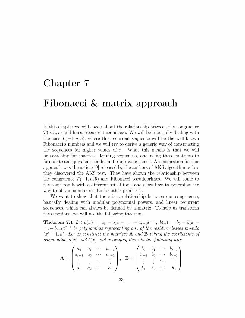
In this chapter we will speak about the relationship between the congruenceT (a, n, r) and linear recurrent sequences. We will be especially dealing withthe case T (−1, n, 5), where this recurrent sequence will be the well-knownFibonacci’s numbers and we will try to derive a generic way of constructingthe sequences for higher values of r. What this means is that we willbe searching for matrices defining sequences, and using these matrices toformulate an equivalent condition for our congruence. An inspiration for thisapproach was the article [9] released by the authors of AKS algorithm beforethey discovered the AKS test. They have shown the relationship betweenthe congruence T (−1, n, 5) and Fibonacci pseudoprimes. We will come tothe same result with a different set of tools and show how to generalize theway to obtain similar results for other prime r’s.
We want to show that there is a relationship between our congruence,basically dealing with modular polynomial powers, and linear recurrentsequences, which can always be defined by a matrix. To help us transformthese notions, we will use the following theorem.
Theorem 7.1 Let a(x) = a0 + a1x + . . . + ar−1xr−1, b(x) = b0 + b1x +
. . .+ br−1xr−1 be polynomials representing any of the residue classes modulo
(xr − 1, n). Let us construct the matrices A and B taking the coefficients ofpolynomials a(x) and b(x) and arranging them in the following way
A =
a0 a1 · · · ar−1
ar−1 a0 · · · ar−2...
... . . . ...a1 a2 · · · a0
, B =
b0 b1 · · · br−1
br−1 b0 · · · br−2...
... . . . ...b1 b2 · · · b0
33
34 CHAPTER 7. FIBONACCI & MATRIX APPROACH
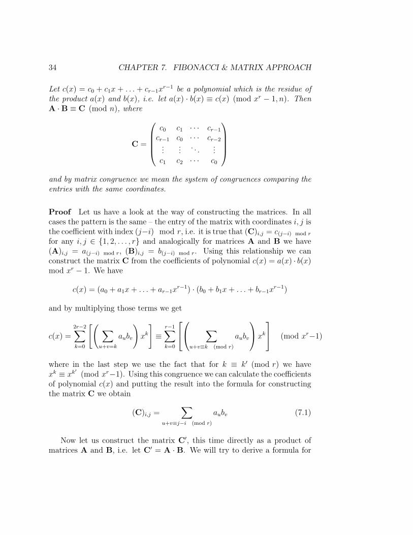
Let c(x) = c0 + c1x + . . . + cr−1xr−1 be a polynomial which is the residue of
the product a(x) and b(x), i.e. let a(x) · b(x) ≡ c(x) (mod xr − 1, n). ThenA ·B ≡ C (mod n), where
C =
c0 c1 · · · cr−1
cr−1 c0 · · · cr−2...
... . . . ...c1 c2 · · · c0
and by matrix congruence we mean the system of congruences comparing theentries with the same coordinates.
Proof Let us have a look at the way of constructing the matrices. In allcases the pattern is the same – the entry of the matrix with coordinates i, j isthe coefficient with index (j−i) mod r, i.e. it is true that (C)i,j = c(j−i) mod r
for any i, j ∈ {1, 2, . . . , r} and analogically for matrices A and B we have(A)i,j = a(j−i) mod r, (B)i,j = b(j−i) mod r. Using this relationship we canconstruct the matrix C from the coefficients of polynomial c(x) = a(x) · b(x)mod xr − 1. We have
c(x) = (a0 + a1x+ . . .+ ar−1xr−1) · (b0 + b1x+ . . .+ br−1x
r−1)
and by multiplying those terms we get
c(x) =2r−2∑k=0
[( ∑u+v=k
aubv
)xk
]≡
r−1∑k=0
∑u+v≡k (mod r)
aubv
xk
(mod xr−1)
where in the last step we use the fact that for k ≡ k′ (mod r) we havexk ≡ xk
′(mod xr−1). Using this congruence we can calculate the coefficients
of polynomial c(x) and putting the result into the formula for constructingthe matrix C we obtain
(C)i,j =∑
u+v≡j−i (mod r)
aubv (7.1)
Now let us construct the matrix C′, this time directly as a product ofmatrices A and B, i.e. let C′ = A · B. We will try to derive a formula for
35
the entry of matrix C′ with coordinates i, j using the usual way of matrixmultiplication. We have
(C′)i,j = (A ·B)i,j =r∑
k=1
(A)i,k · (B)k,j =r∑
k=1
a(k−i) mod r · b(j−k) mod r (7.2)
In the set {1, 2, . . . , r}2 there are exactly r solutions u, v of the congruenceu + v ≡ j − i (mod r), for example if we let the u run through the set{1, . . . , r}, the v is always determined in exactly one way.
Taking a look at the sum in the equation (7.1) we see that it containsexactly these solutions and for choices k = 1, . . . , r in (7.2) we get exactly thesame pairs, because the sum of indexes is always in the residue class (j − i)mod r. With this we have shown that C ≡ C′ (mod n), which concludes theproof of the original theorem. �
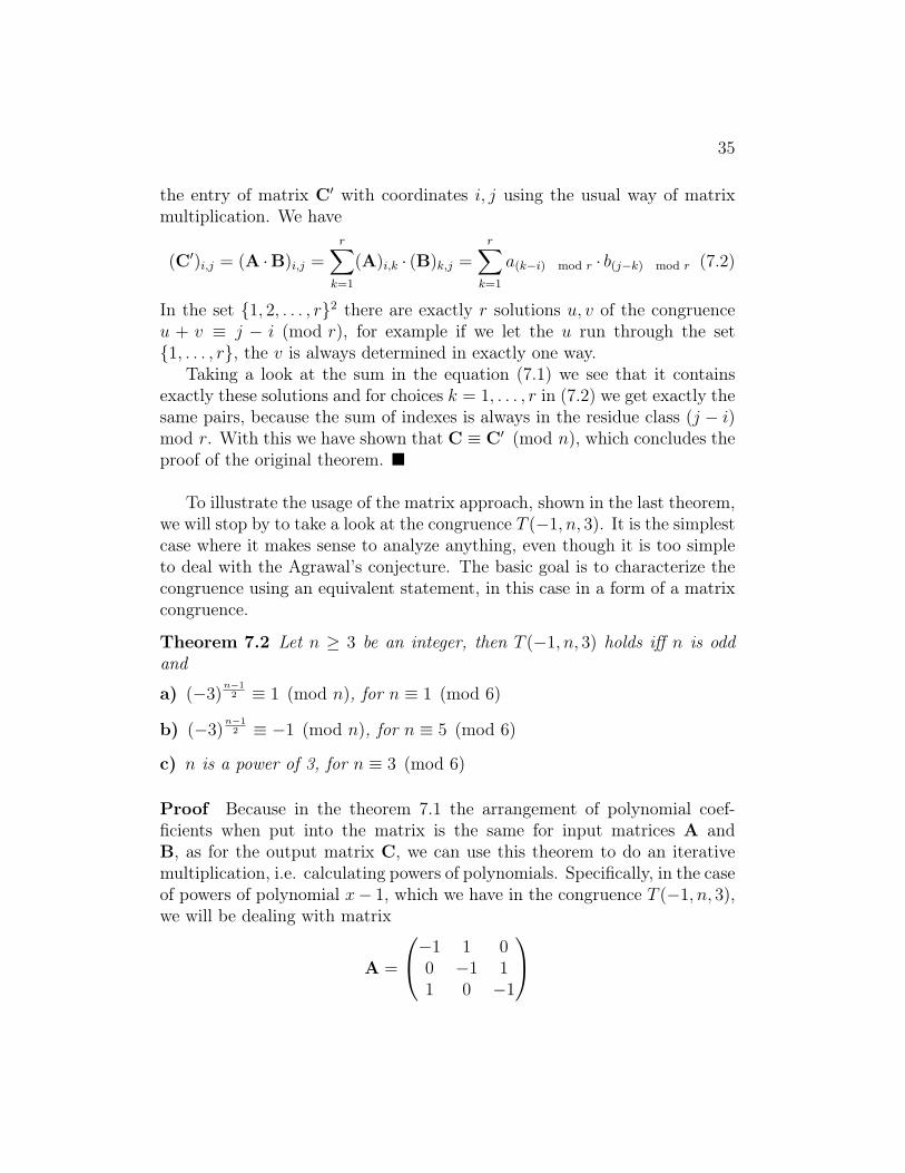
To illustrate the usage of the matrix approach, shown in the last theorem,we will stop by to take a look at the congruence T (−1, n, 3). It is the simplestcase where it makes sense to analyze anything, even though it is too simpleto deal with the Agrawal’s conjecture. The basic goal is to characterize thecongruence using an equivalent statement, in this case in a form of a matrixcongruence.
Theorem 7.2 Let n ≥ 3 be an integer, then T (−1, n, 3) holds iff n is oddand
a) (−3)n−1
2 ≡ 1 (mod n), for n ≡ 1 (mod 6)
b) (−3)n−1
2 ≡ −1 (mod n), for n ≡ 5 (mod 6)
c) n is a power of 3, for n ≡ 3 (mod 6)
Proof Because in the theorem 7.1 the arrangement of polynomial coef-ficients when put into the matrix is the same for input matrices A andB, as for the output matrix C, we can use this theorem to do an iterativemultiplication, i.e. calculating powers of polynomials. Specifically, in the caseof powers of polynomial x− 1, which we have in the congruence T (−1, n, 3),we will be dealing with matrix
A =
−1 1 00 −1 11 0 −1
36 CHAPTER 7. FIBONACCI & MATRIX APPROACH
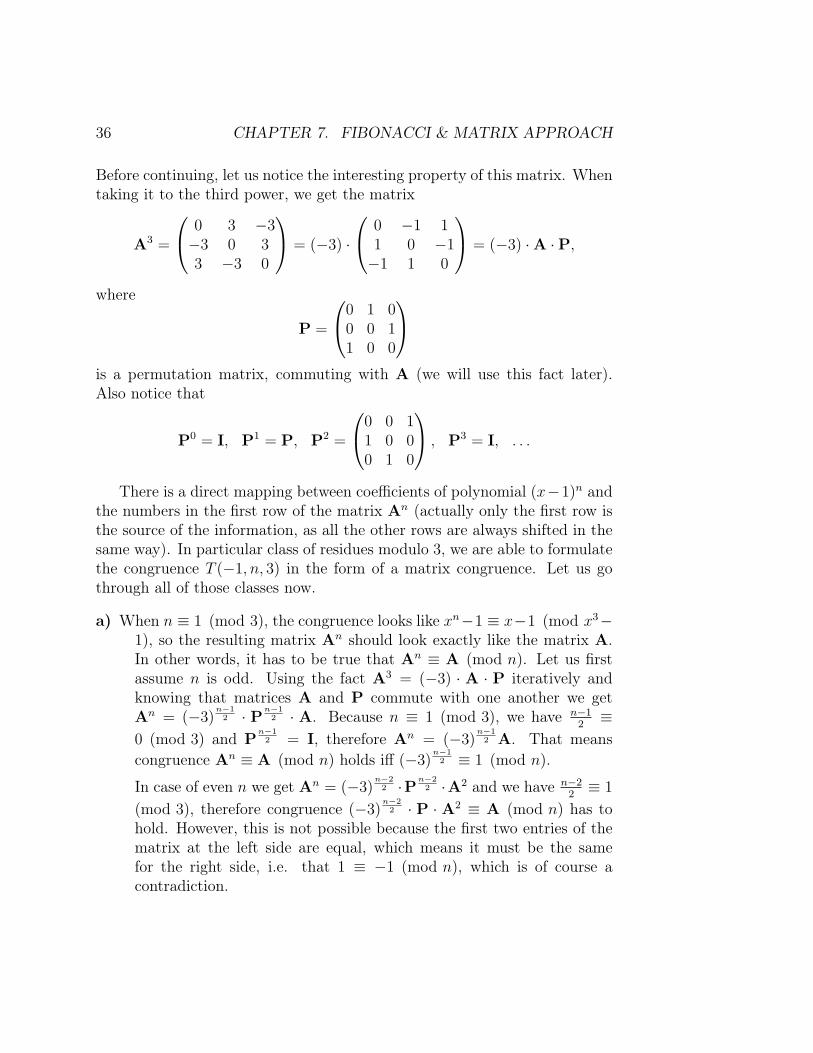
Before continuing, let us notice the interesting property of this matrix. Whentaking it to the third power, we get the matrix
A3 =
0 3 −3−3 0 33 −3 0
= (−3) ·
0 −1 11 0 −1−1 1 0
= (−3) ·A ·P,
where
P =
0 1 00 0 11 0 0
is a permutation matrix, commuting with A (we will use this fact later).Also notice that
P0 = I, P1 = P, P2 =
0 0 11 0 00 1 0
, P3 = I, . . .
There is a direct mapping between coefficients of polynomial (x−1)n andthe numbers in the first row of the matrix An (actually only the first row isthe source of the information, as all the other rows are always shifted in thesame way). In particular class of residues modulo 3, we are able to formulatethe congruence T (−1, n, 3) in the form of a matrix congruence. Let us gothrough all of those classes now.
a) When n ≡ 1 (mod 3), the congruence looks like xn−1 ≡ x−1 (mod x3−1), so the resulting matrix An should look exactly like the matrix A.In other words, it has to be true that An ≡ A (mod n). Let us firstassume n is odd. Using the fact A3 = (−3) · A · P iteratively andknowing that matrices A and P commute with one another we getAn = (−3)
n−12 · Pn−1
2 · A. Because n ≡ 1 (mod 3), we have n−12≡
0 (mod 3) and Pn−1
2 = I, therefore An = (−3)n−1
2 A. That meanscongruence An ≡ A (mod n) holds iff (−3)
n−12 ≡ 1 (mod n).
In case of even n we get An = (−3)n−2
2 ·Pn−22 ·A2 and we have n−2
2≡ 1
(mod 3), therefore congruence (−3)n−2
2 · P · A2 ≡ A (mod n) has tohold. However, this is not possible because the first two entries of thematrix at the left side are equal, which means it must be the samefor the right side, i.e. that 1 ≡ −1 (mod n), which is of course acontradiction.
37
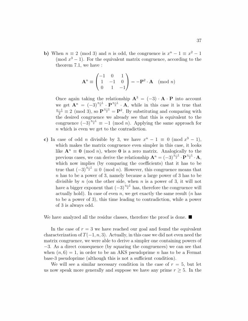
b) When n ≡ 2 (mod 3) and n is odd, the congruence is xn − 1 ≡ x2 − 1(mod x3 − 1). For the equivalent matrix congruence, according to thetheorem 7.1, we have :
An ≡
−1 0 11 −1 00 1 −1
= −P2 ·A (mod n)
Once again taking the relationship A3 = (−3) · A · P into accountwe get An = (−3)
n−12 · Pn−1
2 · A, while in this case it is true thatn−1
2≡ 2 (mod 3), so P
n−12 = P2. By substituting and comparing with
the desired congruence we already see that this is equivalent to thecongruence (−3)
n−12 ≡ −1 (mod n). Applying the same approach for
n which is even we get to the contradiction.
c) In case of odd n divisible by 3, we have xn − 1 ≡ 0 (mod x3 − 1),which makes the matrix congruence even simpler in this case, it lookslike An ≡ 0 (mod n), where 0 is a zero matrix. Analogically to theprevious cases, we can derive the relationship An = (−3)
n−12 ·Pn−1
2 ·A,which now implies (by comparing the coefficients) that it has to betrue that (−3)
n−12 ≡ 0 (mod n). However, this congruence means that
n has to be a power of 3, namely because a large power of 3 has to bedivisible by n (on the other side, when n is a power of 3, it will nothave a bigger exponent that (−3)
n−12 has, therefore the congruence will
actually hold). In case of even n, we get exactly the same result (n hasto be a power of 3), this time leading to contradiction, while a powerof 3 is always odd.
We have analyzed all the residue classes, therefore the proof is done. �
In the case of r = 3 we have reached our goal and found the equivalentcharacterization of T (−1, n, 3). Actually, in this case we did not even need thematrix congruence, we were able to derive a simpler one containing powers of−3. As a direct consequence (by squaring the congruences) we can see thatwhen (n, 6) = 1, in order to be an AKS pseudoprime n has to be a Fermatbase-3 pseudoprime (although this is not a sufficient condition).
We will see a similar necessary condition in the case of r = 5, but letus now speak more generally and suppose we have any prime r ≥ 5. In the
38 CHAPTER 7. FIBONACCI & MATRIX APPROACH
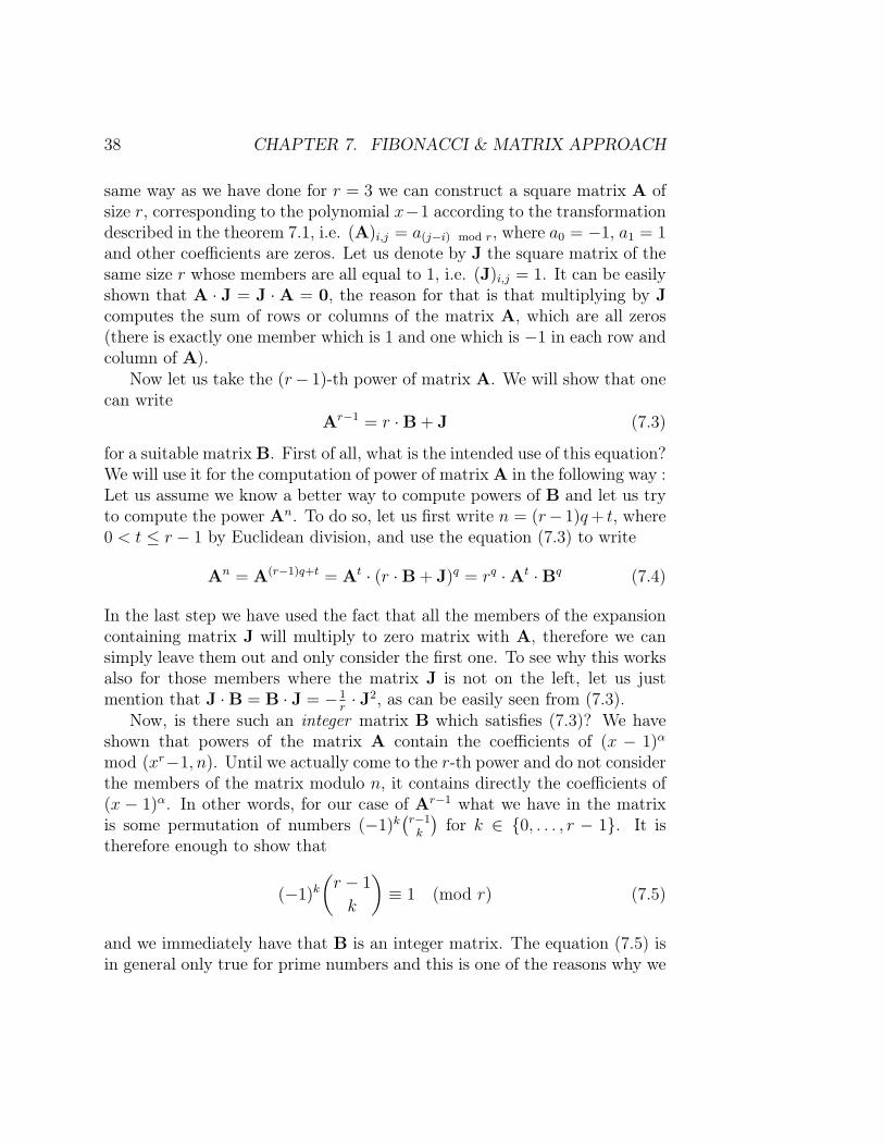
same way as we have done for r = 3 we can construct a square matrix A ofsize r, corresponding to the polynomial x−1 according to the transformationdescribed in the theorem 7.1, i.e. (A)i,j = a(j−i) mod r, where a0 = −1, a1 = 1and other coefficients are zeros. Let us denote by J the square matrix of thesame size r whose members are all equal to 1, i.e. (J)i,j = 1. It can be easilyshown that A · J = J ·A = 0, the reason for that is that multiplying by Jcomputes the sum of rows or columns of the matrix A, which are all zeros(there is exactly one member which is 1 and one which is −1 in each row andcolumn of A).
Now let us take the (r− 1)-th power of matrix A. We will show that onecan write
Ar−1 = r ·B + J (7.3)
for a suitable matrix B. First of all, what is the intended use of this equation?We will use it for the computation of power of matrix A in the following way :Let us assume we know a better way to compute powers of B and let us tryto compute the power An. To do so, let us first write n = (r− 1)q+ t, where0 < t ≤ r − 1 by Euclidean division, and use the equation (7.3) to write
An = A(r−1)q+t = At · (r ·B + J)q = rq ·At ·Bq (7.4)
In the last step we have used the fact that all the members of the expansioncontaining matrix J will multiply to zero matrix with A, therefore we cansimply leave them out and only consider the first one. To see why this worksalso for those members where the matrix J is not on the left, let us justmention that J ·B = B · J = −1
r· J2, as can be easily seen from (7.3).
Now, is there such an integer matrix B which satisfies (7.3)? We haveshown that powers of the matrix A contain the coefficients of (x − 1)α
mod (xr−1, n). Until we actually come to the r-th power and do not considerthe members of the matrix modulo n, it contains directly the coefficients of(x − 1)α. In other words, for our case of Ar−1 what we have in the matrixis some permutation of numbers (−1)k
(r−1k
)for k ∈ {0, . . . , r − 1}. It is
therefore enough to show that
(−1)k(r − 1
k
)≡ 1 (mod r) (7.5)
and we immediately have that B is an integer matrix. The equation (7.5) isin general only true for prime numbers and this is one of the reasons why we
39
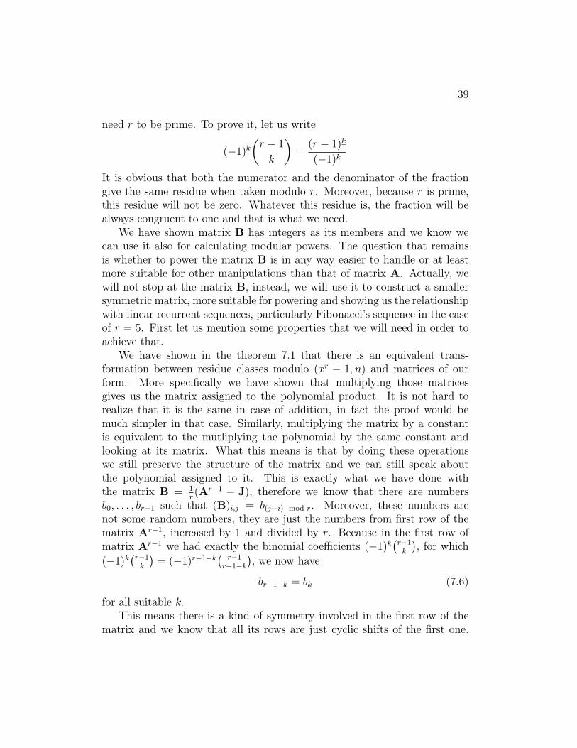
need r to be prime. To prove it, let us write
(−1)k(r − 1
k
)=
(r − 1)k
(−1)k
It is obvious that both the numerator and the denominator of the fractiongive the same residue when taken modulo r. Moreover, because r is prime,this residue will not be zero. Whatever this residue is, the fraction will bealways congruent to one and that is what we need.
We have shown matrix B has integers as its members and we know wecan use it also for calculating modular powers. The question that remainsis whether to power the matrix B is in any way easier to handle or at leastmore suitable for other manipulations than that of matrix A. Actually, wewill not stop at the matrix B, instead, we will use it to construct a smallersymmetric matrix, more suitable for powering and showing us the relationshipwith linear recurrent sequences, particularly Fibonacci’s sequence in the caseof r = 5. First let us mention some properties that we will need in order toachieve that.
We have shown in the theorem 7.1 that there is an equivalent trans-formation between residue classes modulo (xr − 1, n) and matrices of ourform. More specifically we have shown that multiplying those matricesgives us the matrix assigned to the polynomial product. It is not hard torealize that it is the same in case of addition, in fact the proof would bemuch simpler in that case. Similarly, multiplying the matrix by a constantis equivalent to the mutliplying the polynomial by the same constant andlooking at its matrix. What this means is that by doing these operationswe still preserve the structure of the matrix and we can still speak aboutthe polynomial assigned to it. This is exactly what we have done withthe matrix B = 1
r(Ar−1 − J), therefore we know that there are numbers
b0, . . . , br−1 such that (B)i,j = b(j−i) mod r. Moreover, these numbers arenot some random numbers, they are just the numbers from first row of thematrix Ar−1, increased by 1 and divided by r. Because in the first row ofmatrix Ar−1 we had exactly the binomial coefficients (−1)k
(r−1k
), for which
(−1)k(r−1k
)= (−1)r−1−k( r−1
r−1−k
), we now have
br−1−k = bk (7.6)
for all suitable k.This means there is a kind of symmetry involved in the first row of the
matrix and we know that all its rows are just cyclic shifts of the first one.
40 CHAPTER 7. FIBONACCI & MATRIX APPROACH
Although this does not mean that the matrix B itself is symmetric, it is verynear to that. What it needs is just to do a suitable number of cyclic shifts ofrows (or columns, which is in this case effectively the same). This suitablenumber is about a half of the matrix size, for prime r ≥ 3 it would be r+1
2.
Let us introduce a new name for our shifted matrix, let C = B ·P r+12 , where
P is the permutation matrix representing one cyclic shift.The most important thing for us is that we do not lose any power by
taking powers of C instead of B. This means we should be able to calculateBn from Cn quickly and easily. Fortunately, the permutation matrix did notindeed increase the complexity – it commutes with B, it is true that
(B ·Pr+12 )i,j = (P
r+12 ·B)i,j = b( r−1
2+j−i) mod r (7.7)
and we can identify any of its powers easily. This means the only workwe have to do when we have got Cn is to calculate the exponent (−n · r+1
2)
mod r (of the inverse permutation matrix), do one matrix multiplication andwe immediately have the desired result, i.e. the matrix Bn.
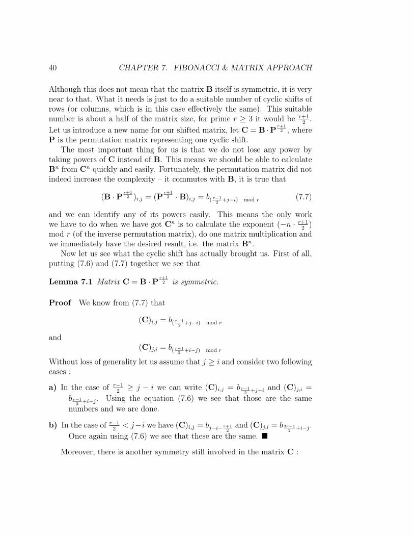
Now let us see what the cyclic shift has actually brought us. First of all,putting (7.6) and (7.7) together we see that
Lemma 7.1 Matrix C = B ·P r+12 is symmetric.
Proof We know from (7.7) that
(C)i,j = b( r−12
+j−i) mod r
and(C)j,i = b( r−1
2+i−j) mod r
Without loss of generality let us assume that j ≥ i and consider two followingcases :
a) In the case of r−12≥ j − i we can write (C)i,j = b r−1
2+j−i and (C)j,i =
b r−12
+i−j. Using the equation (7.6) we see that those are the samenumbers and we are done.
b) In the case of r−12< j−i we have (C)i,j = bj−i− r+1
2and (C)j,i = b 3r−1
2+i−j.
Once again using (7.6) we see that these are the same. �
Moreover, there is another symmetry still involved in the matrix C :
41
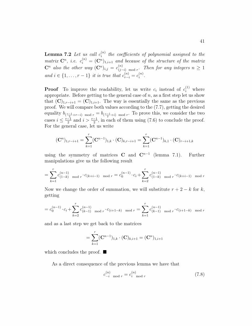
Lemma 7.2 Let us call c(n)i the coefficients of polynomial assigned to the
matrix Cn, i.e. c(n)i = (Cn)1,i+1 and because of the structure of the matrix
Cn also the other way (Cn)i,j = c(n)(j−i) mod r. Then for any integers n ≥ 1
and i ∈ {1, . . . , r − 1} it is true that c(n)r−i = c
(n)i .
Proof To improve the readability, let us write ci instead of c(1)i where
appropriate. Before getting to the general case of n, as a first step let us showthat (C)1,r−i+1 = (C)1,i+1. The way is essentially the same as the previousproof. We will compare both values according to the (7.7), getting the desiredequality b( r−1
2+r−i) mod r = b( r−1
2+i) mod r. To prove this, we consider the two
cases i ≤ r−12
and i > r−12, in each of them using (7.6) to conclude the proof.
For the general case, let us write
(Cn)1,r−i+1 =r∑
k=1
(Cn−1)1,k · (C)k,r−i+1 =r∑
k=1
(Cn−1)k,1 · (C)r−i+1,k
using the symmetry of matrices C and Cn−1 (lemma 7.1). Furthermanipulations give us the following result
=r∑
k=1
c(n−1)(1−k) mod r ·c(k+i−1) mod r = c
(n−1)0 ·ci+
r∑k=2
c(n−1)(1−k) mod r ·c(k+i−1) mod r
Now we change the order of summation, we will substitute r + 2 − k for k,getting
= c(n−1)0 ·ci+
r∑k=2
c(n−1)(k−1) mod r ·c(i+1−k) mod r =
r∑k=1
c(n−1)(k−1) mod r ·c(i+1−k) mod r
and as a last step we get back to the matrices
=r∑
k=1
(Cn−1)1,k · (C)k,i+1 = (Cn)1,i+1
which concludes the proof. �
As a direct consequence of the previous lemma we have that
c(n)−i mod r = c
(n)i mod r (7.8)
42 CHAPTER 7. FIBONACCI & MATRIX APPROACH
which we will use extensively later. We have shown that the matrix Chas some nice properties and symmetries, but we would like to use thesesymmetries to make it easier to calculate its powers. The next step oftransforming the matrix will be the last one, giving us a matrix of less thanhalf the size of C (exactly r−1
2), which will still be symmetric and we can use
it to calculate powers effectively. We will call it the matrix R and define itin the following way :
(R)i,j = (−1)i+j ·(c(j−i) mod r − c(i+j) mod r
)(7.9)
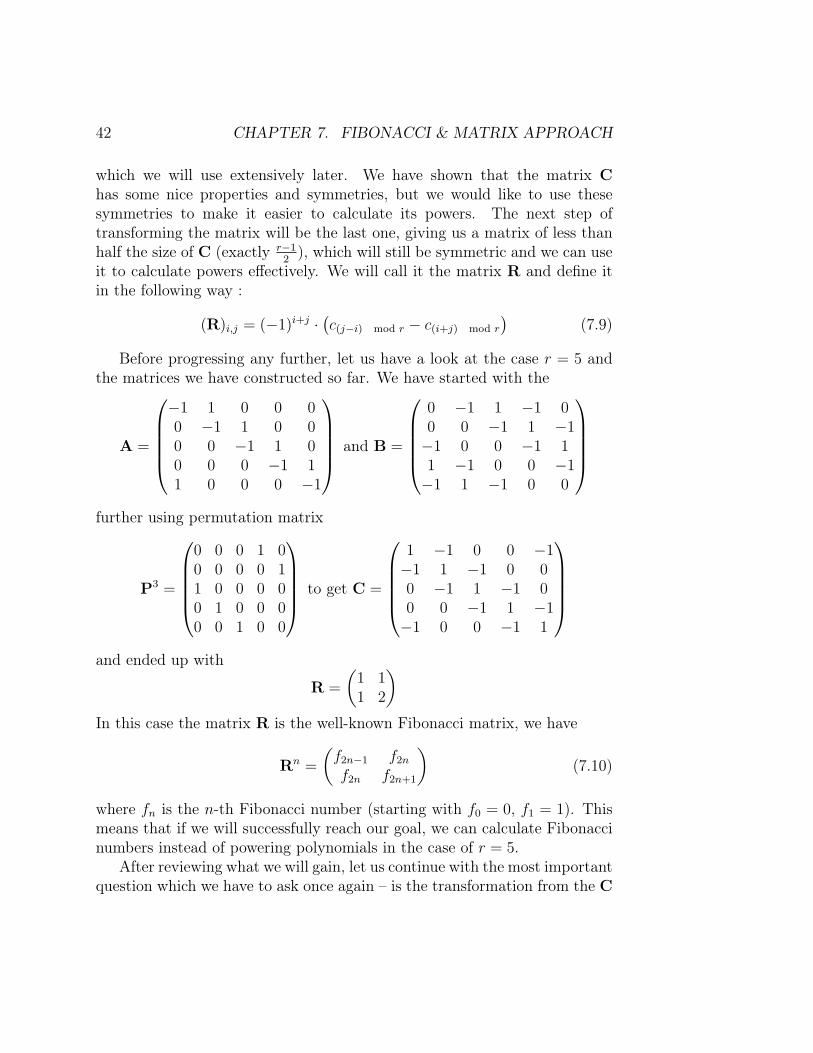
Before progressing any further, let us have a look at the case r = 5 andthe matrices we have constructed so far. We have started with the
A =
−1 1 0 0 00 −1 1 0 00 0 −1 1 00 0 0 −1 11 0 0 0 −1
and B =
0 −1 1 −1 00 0 −1 1 −1−1 0 0 −1 11 −1 0 0 −1−1 1 −1 0 0
further using permutation matrix
P3 =
0 0 0 1 00 0 0 0 11 0 0 0 00 1 0 0 00 0 1 0 0
to get C =
1 −1 0 0 −1−1 1 −1 0 00 −1 1 −1 00 0 −1 1 −1−1 0 0 −1 1
and ended up with
R =
(1 11 2
)In this case the matrix R is the well-known Fibonacci matrix, we have
Rn =
(f2n−1 f2n
f2n f2n+1
)(7.10)
where fn is the n-th Fibonacci number (starting with f0 = 0, f1 = 1). Thismeans that if we will successfully reach our goal, we can calculate Fibonaccinumbers instead of powering polynomials in the case of r = 5.
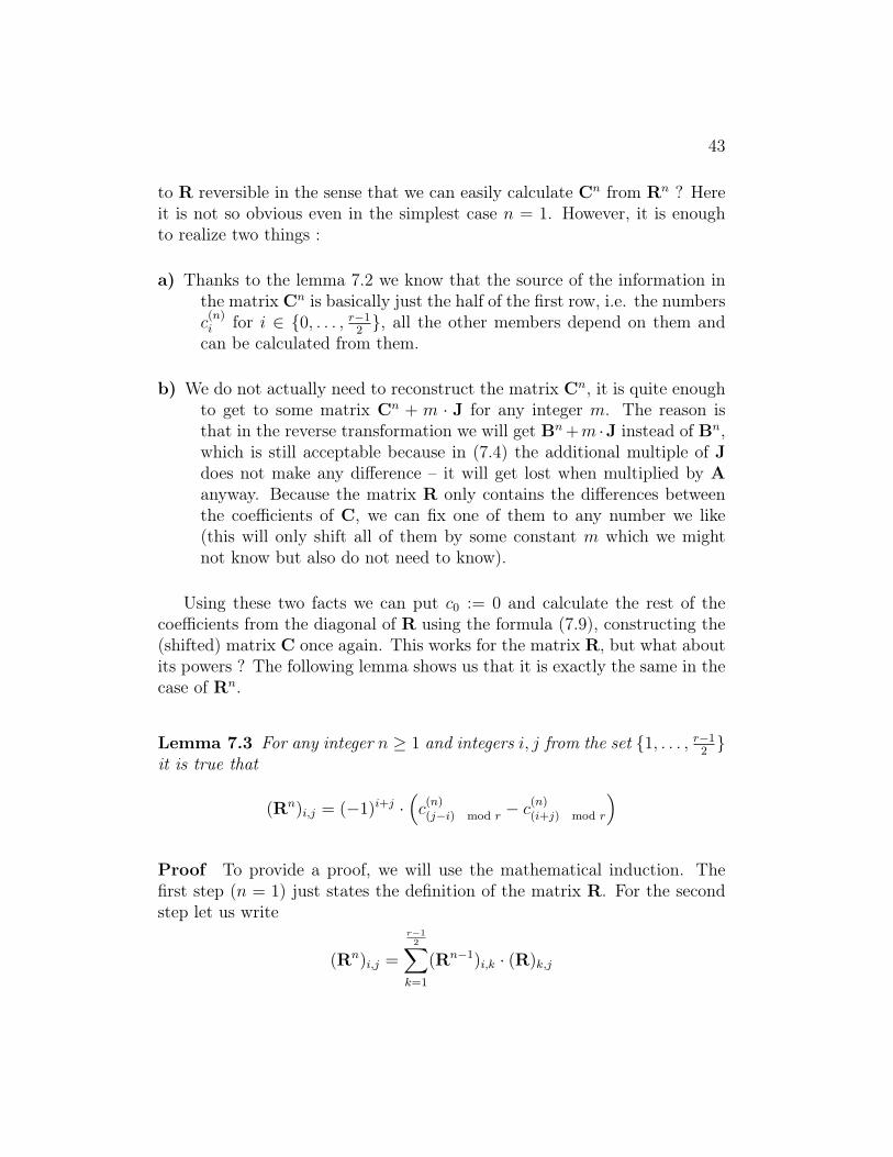
After reviewing what we will gain, let us continue with the most importantquestion which we have to ask once again – is the transformation from the C
43
to R reversible in the sense that we can easily calculate Cn from Rn ? Hereit is not so obvious even in the simplest case n = 1. However, it is enoughto realize two things :
a) Thanks to the lemma 7.2 we know that the source of the information inthe matrix Cn is basically just the half of the first row, i.e. the numbersc(n)i for i ∈ {0, . . . , r−1
2}, all the other members depend on them and
can be calculated from them.
b) We do not actually need to reconstruct the matrix Cn, it is quite enoughto get to some matrix Cn + m · J for any integer m. The reason isthat in the reverse transformation we will get Bn+m ·J instead of Bn,which is still acceptable because in (7.4) the additional multiple of Jdoes not make any difference – it will get lost when multiplied by Aanyway. Because the matrix R only contains the differences betweenthe coefficients of C, we can fix one of them to any number we like(this will only shift all of them by some constant m which we mightnot know but also do not need to know).
Using these two facts we can put c0 := 0 and calculate the rest of thecoefficients from the diagonal of R using the formula (7.9), constructing the(shifted) matrix C once again. This works for the matrix R, but what aboutits powers ? The following lemma shows us that it is exactly the same in thecase of Rn.
Lemma 7.3 For any integer n ≥ 1 and integers i, j from the set {1, . . . , r−12}
it is true that
(Rn)i,j = (−1)i+j ·(c(n)(j−i) mod r − c
(n)(i+j) mod r
)Proof To provide a proof, we will use the mathematical induction. Thefirst step (n = 1) just states the definition of the matrix R. For the secondstep let us write
(Rn)i,j =
r−12∑
k=1
(Rn−1)i,k · (R)k,j
44 CHAPTER 7. FIBONACCI & MATRIX APPROACH
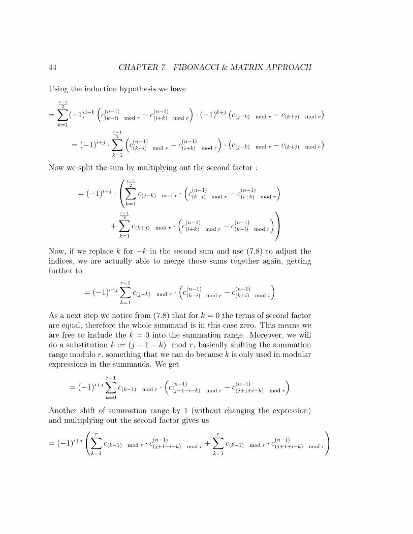
Using the induction hypothesis we have
=
r−12∑
k=1
(−1)i+k(c(n−1)(k−i) mod r − c
(n−1)(i+k) mod r
)· (−1)k+j
(c(j−k) mod r − c(k+j) mod r
)= (−1)i+j ·
r−12∑
k=1
(c(n−1)(k−i) mod r − c
(n−1)(i+k) mod r
)·(c(j−k) mod r − c(k+j) mod r
)Now we split the sum by multiplying out the second factor :
= (−1)i+j ·
r−12∑
k=1
c(j−k) mod r ·(c(n−1)(k−i) mod r − c
(n−1)(i+k) mod r
)
+
r−12∑
k=1
c(k+j) mod r ·(c(n−1)(i+k) mod r − c
(n−1)(k−i) mod r
)Now, if we replace k for −k in the second sum and use (7.8) to adjust theindices, we are actually able to merge those sums together again, gettingfurther to
= (−1)i+jr−1∑k=1
c(j−k) mod r ·(c(n−1)(k−i) mod r − c
(n−1)(k+i) mod r
)As a next step we notice from (7.8) that for k = 0 the terms of second factorare equal, therefore the whole summand is in this case zero. This means weare free to include the k = 0 into the summation range. Moreover, we willdo a substitution k := (j + 1− k) mod r, basically shifting the summationrange modulo r, something that we can do because k is only used in modularexpressions in the summands. We get
= (−1)i+jr−1∑k=0
c(k−1) mod r ·(c(n−1)(j+1−i−k) mod r − c
(n−1)(j+1+i−k) mod r
)Another shift of summation range by 1 (without changing the expression)and multiplying out the second factor gives us
= (−1)i+j
(r∑
k=1
c(k−1) mod r · c(n−1)(j+1−i−k) mod r +
r∑k=1
c(k−1) mod r · c(n−1)(j+1+i−k) mod r
)
45
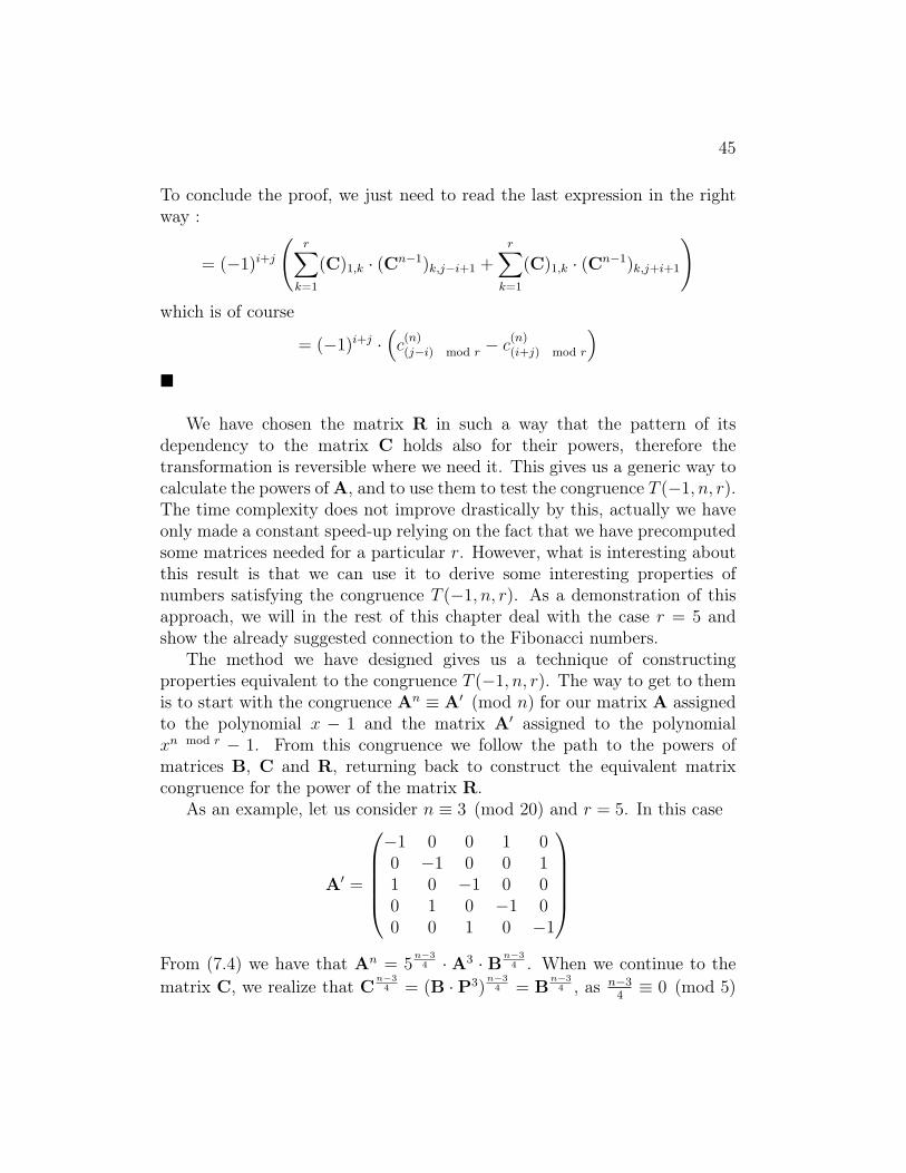
To conclude the proof, we just need to read the last expression in the rightway :
= (−1)i+j
(r∑
k=1
(C)1,k · (Cn−1)k,j−i+1 +r∑
k=1
(C)1,k · (Cn−1)k,j+i+1
)which is of course
= (−1)i+j ·(c(n)(j−i) mod r − c
(n)(i+j) mod r
)�
We have chosen the matrix R in such a way that the pattern of itsdependency to the matrix C holds also for their powers, therefore thetransformation is reversible where we need it. This gives us a generic way tocalculate the powers of A, and to use them to test the congruence T (−1, n, r).The time complexity does not improve drastically by this, actually we haveonly made a constant speed-up relying on the fact that we have precomputedsome matrices needed for a particular r. However, what is interesting aboutthis result is that we can use it to derive some interesting properties ofnumbers satisfying the congruence T (−1, n, r). As a demonstration of thisapproach, we will in the rest of this chapter deal with the case r = 5 andshow the already suggested connection to the Fibonacci numbers.
The method we have designed gives us a technique of constructingproperties equivalent to the congruence T (−1, n, r). The way to get to themis to start with the congruence An ≡ A′ (mod n) for our matrix A assignedto the polynomial x − 1 and the matrix A′ assigned to the polynomialxn mod r − 1. From this congruence we follow the path to the powers ofmatrices B, C and R, returning back to construct the equivalent matrixcongruence for the power of the matrix R.
As an example, let us consider n ≡ 3 (mod 20) and r = 5. In this case
A′ =
−1 0 0 1 00 −1 0 0 11 0 −1 0 00 1 0 −1 00 0 1 0 −1
From (7.4) we have that An = 5
n−34 ·A3 · Bn−3
4 . When we continue to thematrix C, we realize that C
n−34 = (B · P3)
n−34 = B
n−34 , as n−3
4≡ 0 (mod 5)
46 CHAPTER 7. FIBONACCI & MATRIX APPROACH
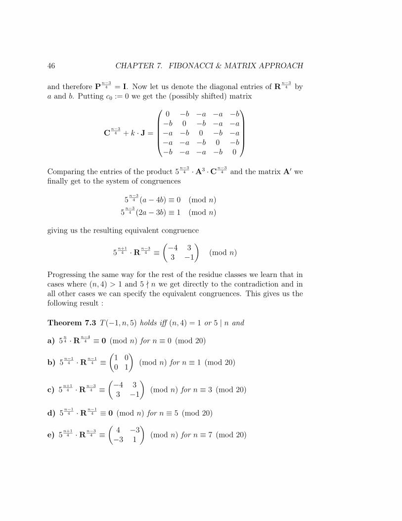
and therefore Pn−3
4 = I. Now let us denote the diagonal entries of Rn−3
4 bya and b. Putting c0 := 0 we get the (possibly shifted) matrix
Cn−3
4 + k · J =
0 −b −a −a −b−b 0 −b −a −a−a −b 0 −b −a−a −a −b 0 −b−b −a −a −b 0
Comparing the entries of the product 5
n−34 ·A3 ·Cn−3
4 and the matrix A′ wefinally get to the system of congruences
5n−3
4 (a− 4b) ≡ 0 (mod n)
5n−3
4 (2a− 3b) ≡ 1 (mod n)
giving us the resulting equivalent congruence
5n+1
4 ·Rn−3
4 ≡(−4 33 −1
)(mod n)
Progressing the same way for the rest of the residue classes we learn that incases where (n, 4) > 1 and 5 - n we get directly to the contradiction and inall other cases we can specify the equivalent congruences. This gives us thefollowing result :
Theorem 7.3 T (−1, n, 5) holds iff (n, 4) = 1 or 5 | n and
a) 5n4 ·Rn−4
4 ≡ 0 (mod n) for n ≡ 0 (mod 20)
b) 5n−1
4 ·Rn−14 ≡
(1 00 1
)(mod n) for n ≡ 1 (mod 20)
c) 5n+1
4 ·Rn−34 ≡
(−4 33 −1
)(mod n) for n ≡ 3 (mod 20)
d) 5n−1
4 ·Rn−14 ≡ 0 (mod n) for n ≡ 5 (mod 20)
e) 5n+1
4 ·Rn−34 ≡
(4 −3−3 1
)(mod n) for n ≡ 7 (mod 20)
47
f) 5n−1
4 ·Rn−14 ≡
(−1 00 −1
)(mod n) for n ≡ 9 (mod 20)
g) 5n−2
4 ·Rn−24 ≡ 0 (mod n) for n ≡ 10 (mod 20)
h) 5n+1
4 ·Rn−34 ≡
(−3 11 −2
)(mod n) for n ≡ 11 (mod 20)
i) 5n−1
4 ·Rn−14 ≡
(1 −1−1 0
)(mod n) for n ≡ 13 (mod 20)
j) 5n+1
4 ·Rn−34 ≡ 0 (mod n) for n ≡ 15 (mod 20)
k) 5n−1
4 ·Rn−14 ≡
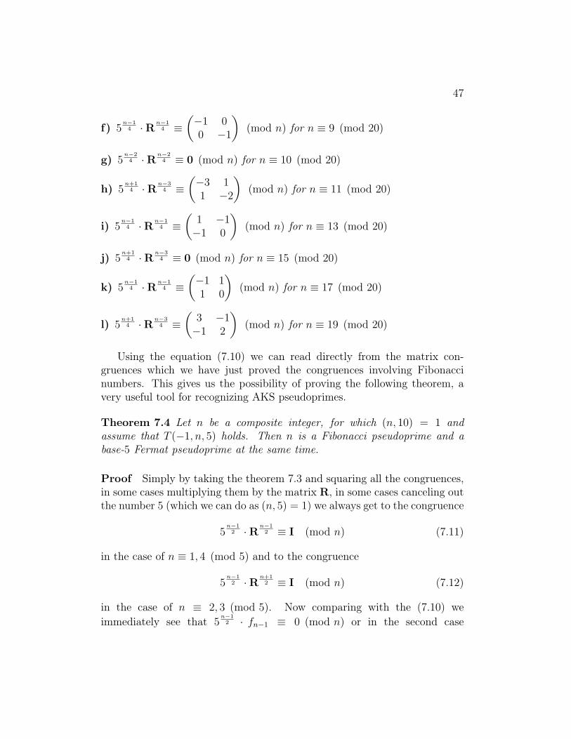
(−1 11 0
)(mod n) for n ≡ 17 (mod 20)
l) 5n+1
4 ·Rn−34 ≡
(3 −1−1 2
)(mod n) for n ≡ 19 (mod 20)
Using the equation (7.10) we can read directly from the matrix con-gruences which we have just proved the congruences involving Fibonaccinumbers. This gives us the possibility of proving the following theorem, avery useful tool for recognizing AKS pseudoprimes.
Theorem 7.4 Let n be a composite integer, for which (n, 10) = 1 andassume that T (−1, n, 5) holds. Then n is a Fibonacci pseudoprime and abase-5 Fermat pseudoprime at the same time.
Proof Simply by taking the theorem 7.3 and squaring all the congruences,in some cases multiplying them by the matrix R, in some cases canceling outthe number 5 (which we can do as (n, 5) = 1) we always get to the congruence
5n−1
2 ·Rn−1
2 ≡ I (mod n) (7.11)
in the case of n ≡ 1, 4 (mod 5) and to the congruence
5n−1
2 ·Rn+1
2 ≡ I (mod n) (7.12)
in the case of n ≡ 2, 3 (mod 5). Now comparing with the (7.10) weimmediately see that 5
n−12 · fn−1 ≡ 0 (mod n) or in the second case
48 CHAPTER 7. FIBONACCI & MATRIX APPROACH
5n−1
2 · fn+1 ≡ 0 (mod n). However, because (n, 5) = 1, this means thatfn−1 ≡ 0 (mod n) or fn+1 ≡ 0 (mod n) respectively, and that is exactlywhat we wanted to prove in the first place. For the second part of our proofwe will use the determinant of the matrix R. Its value is exactly 1, thatmeans also any power of R has a determinant of 1. What this means is thatthe following equation is true
f2k−1 · f2k+1 = f 22k + 1 (7.13)
for any k. Now, comparing the entries of matrices in (7.11) we see that5
n−12 · fn−2 ≡ 1 (mod n), as well as 5
n−12 · fn ≡ 1 (mod n). Multiplying these
together and using (7.13) we see that 5n−1 ≡ 1 (mod n), i.e. the number n isa base-5 Fermat pseudoprime. Analogically comparing the entries of matricesin (7.12) we have 5
n−12 · fn ≡ 1 (mod n), as well as 5
n−12 · fn+2 ≡ 1 (mod n),
which multiplies to 5n−1 ≡ 1 (mod n) when taking (7.13) into consideration.�
The last theorem showed us that when searching for AKS pseudoprimesfor r = 5, we can start with Fibonacci pseudoprimes and base-5 Fermatpseudoprimes, which means we can further investigate their properties andmaybe derive a faster method than we would have just for AKS pseudoprimes.Unfortunately, we have used congruence squaring and multiplying in theproof and therefore lost the equivalence, which means that finding sucha number n that n ≡ 2, 3 (mod 5) and n is Fibonacci pseudoprime andbase-5 pseudoprime at the same time may not necessarily bring us to thecounterexample for the Agrawal’s conjecture, on the other way if there is nosuch number we know that at least for r = 5 we do not have to search anylonger.
Chapter 8
Experimental data
In this last chapter we will present some empirical results from experimentswe have made based on the theoretical observations from the previouschapters. Our goal was to collect some useful statistics suggesting how near orfar are we from finding a counterexample to the Agrawal’s conjecture and tocollect some data that may help in the future search for the counterexample.Although most of these experiments were based on the proved results, theapproach remains rather heuristic as we only have some indications but noevidence that there is any such counterexample.
In the text [9], authors stated that they have made a search up to 1011
for a composite n that would satisfy the congruence T (−1, n, 5) and n ≡ 2, 3(mod 5) at the same time. For other primes r ≤ 100 they have come upto 1010 with the same negative result (i.e. it was always true that n2 ≡ 1(mod r)). In [13] authors provide a proof for the theorem 5.1, afterwardsstating estimations based on heuristic calculations using analytical numbertheory to conclude that there should be a constant, a lower bound for therange where the counterexamples are frequent enough.
Looking at their result it was not difficult to see that although notexplicitly mentioning that, they are dealing with a subset of Carmichaelnumbers. On the other hand, the Carmichael numbers are a point of interestfor many mathematicians, amongst all maybe most significantly RichardPinch, who has in the last 15 years collected all the Carmichael numbersup to 1021 and some lists of pseudoprimes as well (see e.g. [15]). We haveused a publicly available subset up to 1018 to perform some experiments,results of which we present here. We also asked Mr. Pinch for the rest of thedata and we will continue with the experiments as soon as he provides them.
49
50 CHAPTER 8. EXPERIMENTAL DATA
As a part of a school project in the course of computer algebra, the authorof this work has used the software Maple in version 11 to perform some basicsearch in range 〈1, 1016〉 and at first it seemed we have discovered somecounterexamples even in this range. After further tests, we have found outthat the reason why our algorithm reported those numbers as positive was abug in the Maple’s function isprime which uses some randomized primalitytests and in the documentation they wrote that
No counterexample is known and it has been conjectured that such a counterexample must be hundreds of digits long.
Actually, we have found the following three Carmichael numbers
43438471758571 = 5503 · 8123 · 971759
54165858332251 = 14071 · 32831 · 117251
367826207971951 = 10531 · 94771 · 368551
that were falsely identified as prime by Maple. We reported this to thesupport team and they have admitted this is a bug.
In the version 12 of Maple this bug is already fixed, but we have decided,most importantly for performance reasons, to try out some other frameworksthat are more suitable for our purposes. We have found two relevant libraries– LiDIA and NTL (see [8] and [18]) and have decided for the second oneas a main tool for our computations. First, let us have a look at themost interesting question – taking the theorem 5.1, how many Carmichaelnumbers satisfy the individual conditions. As we are dealing with Carmichaelnumbers, the Korselt’s criterion tells us that all of them are square-free andthe condition c) is satisfied automatically. Therefore it only makes sense toask about the conditions from a), b) and d). The following table shows theresults :
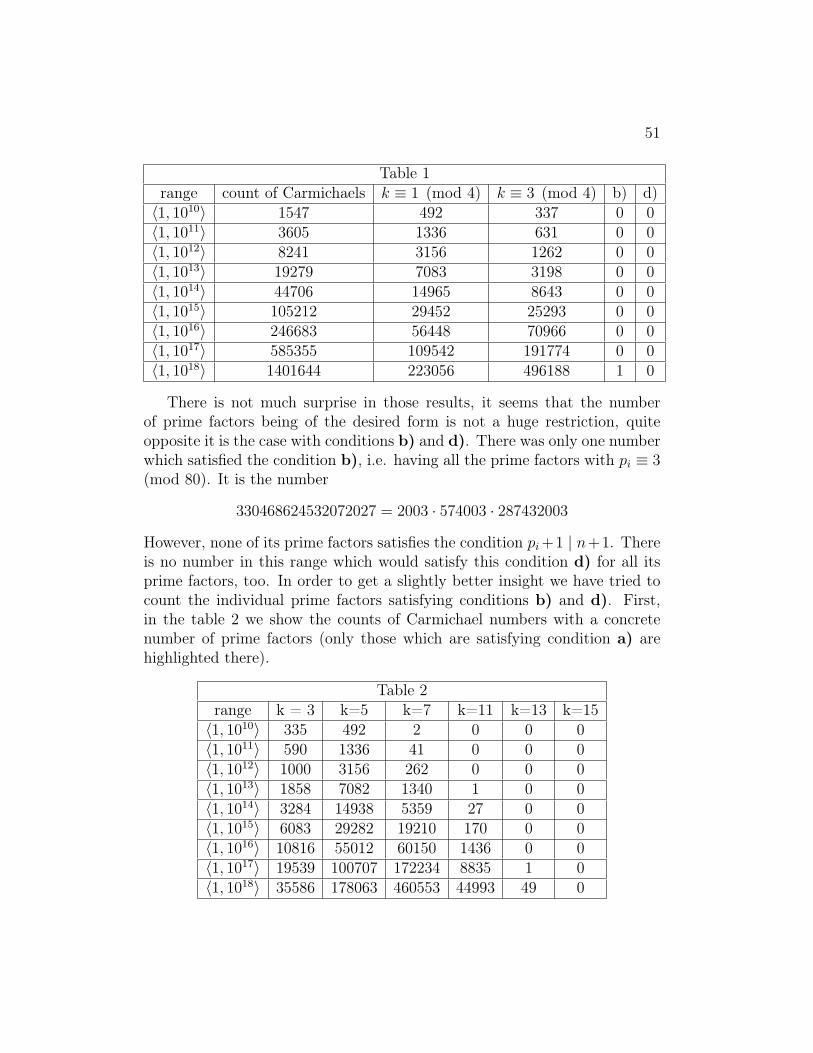
51
Table 1range count of Carmichaels k ≡ 1 (mod 4) k ≡ 3 (mod 4) b) d)〈1, 1010〉 1547 492 337 0 0〈1, 1011〉 3605 1336 631 0 0〈1, 1012〉 8241 3156 1262 0 0〈1, 1013〉 19279 7083 3198 0 0〈1, 1014〉 44706 14965 8643 0 0〈1, 1015〉 105212 29452 25293 0 0〈1, 1016〉 246683 56448 70966 0 0〈1, 1017〉 585355 109542 191774 0 0〈1, 1018〉 1401644 223056 496188 1 0
There is not much surprise in those results, it seems that the numberof prime factors being of the desired form is not a huge restriction, quiteopposite it is the case with conditions b) and d). There was only one numberwhich satisfied the condition b), i.e. having all the prime factors with pi ≡ 3(mod 80). It is the number
330468624532072027 = 2003 · 574003 · 287432003
However, none of its prime factors satisfies the condition pi+1 | n+1. Thereis no number in this range which would satisfy this condition d) for all itsprime factors, too. In order to get a slightly better insight we have tried tocount the individual prime factors satisfying conditions b) and d). First,in the table 2 we show the counts of Carmichael numbers with a concretenumber of prime factors (only those which are satisfying condition a) arehighlighted there).
Table 2range k = 3 k=5 k=7 k=11 k=13 k=15〈1, 1010〉 335 492 2 0 0 0〈1, 1011〉 590 1336 41 0 0 0〈1, 1012〉 1000 3156 262 0 0 0〈1, 1013〉 1858 7082 1340 1 0 0〈1, 1014〉 3284 14938 5359 27 0 0〈1, 1015〉 6083 29282 19210 170 0 0〈1, 1016〉 10816 55012 60150 1436 0 0〈1, 1017〉 19539 100707 172234 8835 1 0〈1, 1018〉 35586 178063 460553 44993 49 0
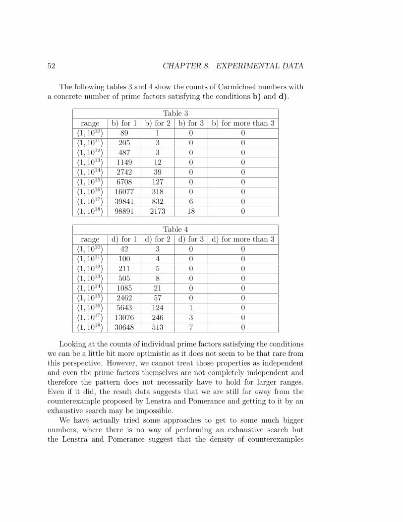
52 CHAPTER 8. EXPERIMENTAL DATA
The following tables 3 and 4 show the counts of Carmichael numbers witha concrete number of prime factors satisfying the conditions b) and d).
Table 3range b) for 1 b) for 2 b) for 3 b) for more than 3〈1, 1010〉 89 1 0 0〈1, 1011〉 205 3 0 0〈1, 1012〉 487 3 0 0〈1, 1013〉 1149 12 0 0〈1, 1014〉 2742 39 0 0〈1, 1015〉 6708 127 0 0〈1, 1016〉 16077 318 0 0〈1, 1017〉 39841 832 6 0〈1, 1018〉 98891 2173 18 0
Table 4range d) for 1 d) for 2 d) for 3 d) for more than 3〈1, 1010〉 42 3 0 0〈1, 1011〉 100 4 0 0〈1, 1012〉 211 5 0 0〈1, 1013〉 505 8 0 0〈1, 1014〉 1085 21 0 0〈1, 1015〉 2462 57 0 0〈1, 1016〉 5643 124 1 0〈1, 1017〉 13076 246 3 0〈1, 1018〉 30648 513 7 0
Looking at the counts of individual prime factors satisfying the conditionswe can be a little bit more optimistic as it does not seem to be that rare fromthis perspective. However, we cannot treat those properties as independentand even the prime factors themselves are not completely independent andtherefore the pattern does not necessarily have to hold for larger ranges.Even if it did, the result data suggests that we are still far away from thecounterexample proposed by Lenstra and Pomerance and getting to it by anexhaustive search may be impossible.
We have actually tried some approaches to get to some much biggernumbers, where there is no way of performing an exhaustive search butthe Lenstra and Pomerance suggest that the density of counterexamples
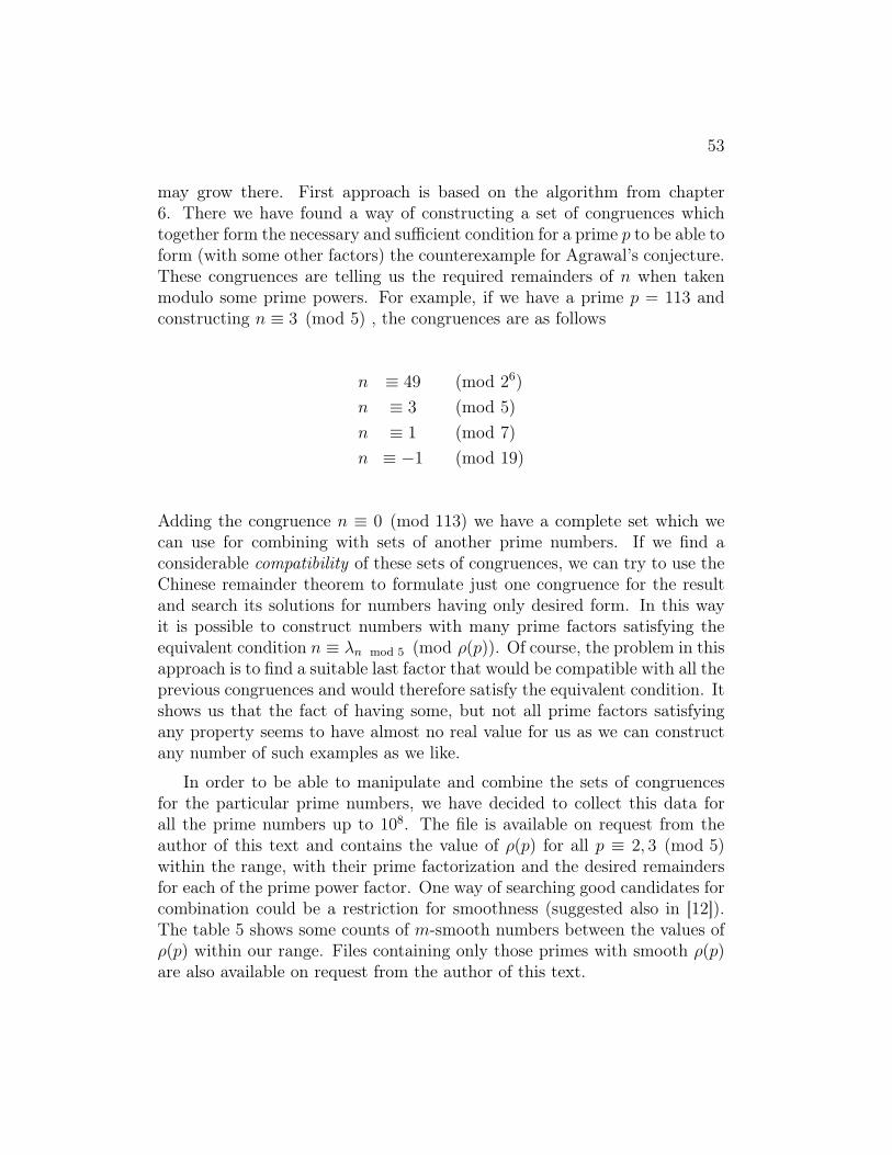
53
may grow there. First approach is based on the algorithm from chapter6. There we have found a way of constructing a set of congruences whichtogether form the necessary and sufficient condition for a prime p to be able toform (with some other factors) the counterexample for Agrawal’s conjecture.These congruences are telling us the required remainders of n when takenmodulo some prime powers. For example, if we have a prime p = 113 andconstructing n ≡ 3 (mod 5) , the congruences are as follows
n ≡ 49 (mod 26)
n ≡ 3 (mod 5)
n ≡ 1 (mod 7)
n ≡ −1 (mod 19)
Adding the congruence n ≡ 0 (mod 113) we have a complete set which wecan use for combining with sets of another prime numbers. If we find aconsiderable compatibility of these sets of congruences, we can try to use theChinese remainder theorem to formulate just one congruence for the resultand search its solutions for numbers having only desired form. In this wayit is possible to construct numbers with many prime factors satisfying theequivalent condition n ≡ λn mod 5 (mod ρ(p)). Of course, the problem in thisapproach is to find a suitable last factor that would be compatible with all theprevious congruences and would therefore satisfy the equivalent condition. Itshows us that the fact of having some, but not all prime factors satisfyingany property seems to have almost no real value for us as we can constructany number of such examples as we like.
In order to be able to manipulate and combine the sets of congruencesfor the particular prime numbers, we have decided to collect this data forall the prime numbers up to 108. The file is available on request from theauthor of this text and contains the value of ρ(p) for all p ≡ 2, 3 (mod 5)within the range, with their prime factorization and the desired remaindersfor each of the prime power factor. One way of searching good candidates forcombination could be a restriction for smoothness (suggested also in [12]).The table 5 shows some counts of m-smooth numbers between the values ofρ(p) within our range. Files containing only those primes with smooth ρ(p)are also available on request from the author of this text.
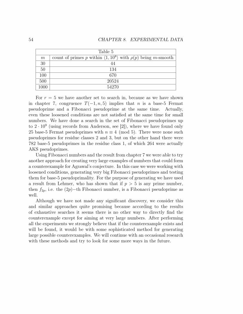
54 CHAPTER 8. EXPERIMENTAL DATA
Table 5m count of primes p within 〈1, 108〉 with ρ(p) being m-smooth30 4450 134100 670500 205241000 54270
For r = 5 we have another set to search in, because as we have shownin chapter 7, congruence T (−1, n, 5) implies that n is a base-5 Fermatpseudoprime and a Fibonacci pseudoprime at the same time. Actually,even these loosened conditions are not satisfied at the same time for smallnumbers. We have done a search in the set of Fibonacci pseudoprimes upto 2 · 109 (using records from Anderson, see [2]), where we have found only25 base-5 Fermat pseudoprimes with n ≡ 4 (mod 5). There were none suchpseudoprimes for residue classes 2 and 3, but on the other hand there were782 base-5 pseudoprimes in the residue class 1, of which 264 were actuallyAKS pseudoprimes.
Using Fibonacci numbers and the result from chapter 7 we were able to tryanother approach for creating very large examples of numbers that could forma counterexample for Agrawal’s conjecture. In this case we were working withloosened conditions, generating very big Fibonacci pseudoprimes and testingthem for base-5 pseudoprimality. For the purpose of generating we have useda result from Lehmer, who has shown that if p > 5 is any prime number,then f2p, i.e. the (2p)−th Fibonacci number, is a Fibonacci pseudoprime aswell.
Although we have not made any significant discovery, we consider thisand similar approaches quite promising because according to the resultsof exhaustive searches it seems there is no other way to directly find thecounterexample except for aiming at very large numbers. After performingall the experiments we strongly believe that if the counterexample exists andwill be found, it would be with some sophisticated method for generatinglarge possible counterexamples. We will continue with an occasional researchwith these methods and try to look for some more ways in the future.
Chapter 9
Conclusion
A couple of years ago the problem of primes recognition was still not knownto belong into the polynomial class of algorithms. Even then we already hada lot of algorithms for primality testing, using very sophisticated ideas andsome of them were really fast. Each of them had some flaw – from some smallerror probability, depending on an unproved conjecture to being polynomialonly on some inputs or being slightly more than polynomial on all of them.
Although these algorithms were not perfect from a strict point of view,some of them were very elegant and easily understandable, which made themintelligible and usable both to mathematicians and computer scientists. Afterall, only a couple of decades has passed from the discovery of RSA whichlaunched the heavy usage of number theory in cryptography and made itattractive to the computer scientists, not only as a theoretical tool, but forvery practical reasons, too.
The year 2002 has brought a breakthrough in this area, the algorithmAKS which is also an elegant and easy to understand and does not have anytheoretical drawbacks. The only problem still present is that although beinga satisfactory solution for computer scientists, it is not much of a use forpractical applications, e.g. for generating primes for keys. The reason forthat is of course that even though it is polynomial, the large exponent stillmakes it too slow. In our thesis we have tried to research some of its aspectsin order to make it faster or show that some of the suggested ways to makeit faster do not work and we should look somewhere else.
We have started with an overview of primality testing algorithmsincluding the AKS algorithm in order to give the reader some feeling aboutit and prepare some necessary terms. We presented the Agrawal’s conjecture
55
56 CHAPTER 9. CONCLUSION
as a central point of interest for the following story. As a next step we havedemonstrated the use of combinatoric methods to deal with modular sumsin the binomial expansion. In our particular problem this approach was aninteresting way of how to prove the theorem and gain a better insight to thestructure of objects we are dealing with. We have also provided the algebraicproof as an alternative, just to compare and see the difference.
The main idea of these chapters was to explore the choices of theparameters in the AKS congruence and in some way show the reason forthe formulation of the Agrawal’s conjecture. In addition to the Carmichaelnumbers, we have shown that Mersenne numbers of special form, whichexistence is guaranteed by the Sophie-Germain prime conjecture, maypossibly represent an infinite sequence of numbers making troubles to theAKS congruence.
We have then presented the Lenstra-Pomerance heuristic as an argumentagainst Agrawal’s conjecture, we have provided an alternative proof for thetheorem that is a base of the heuristic, adding case k = 3, which wasmentioned as an exercise in the original article. The way of proving it alsoprovided us with an algorithm to search for parameters needed to test theAKS congruence directly in the case of r = 5.
In the next chapter, we have developed tools involving matrix exponen-tiation and transformations into smaller symmetric matrices of recurrentsequences, giving us yet another way of testing the congruence, in this casemore generic one which works also without knowing the prime factorizationof the input or putting any restrictions to it. More importantly, we havegeneralized the previously known way of expressing the relationship betweenthe recurrent sequences (e.g. Fibonacci numbers) and the AKS congruence.
As a conclusion, we have made some concrete experiments to try out theapproaches that we have invented and provide some statistics which wouldgive us a feeling of how far away is the answer to the questions we have askedat the begining. We have collected some data that can be used as a basis offurther research in this area.
We believe that we have opened some new possibilities and brought newideas which could eventually lead to the discovery of the counterexamples orproofs of the mentioned conjecture or some other interesting results relatedto the AKS test and hope that they were inspiring for the reader. We lookforward to any advances in this area and will try to contribute to it in thefuture.
Bibliography
[1] Agrawal M., Kayal N., Saxena N.: PRIMES is in P. Annals ofMathematics 160(2), 2004, p. 781–793.
[2] Anderson P.: Fibonacci pseudoprimes up to 2217967487. (data file)http://www.cs.rit.edu/usr/local/pub/pga/fibonacci_pp
[3] Bernstein D.: Detecting perfect powers in essentially linear time.Mathematics of computation 223, 1998, p.1253-1283.
[4] Bernstein D.: Distinguishing prime numbers from composite numbers:the state of the art in 2004. (unpublished)http://cr.yp.to/papers.html#prime2004
[5] Crandall R., Pomerance C.: Prime Numbers - A computationalperspective. Springer-Verlag, New York, 2001.
[6] Dietzfelbinger M.: Primality testing in polynomial time. Springer-Verlag, Berlin, 2004.
[7] Galway W.: Pseudoprimes up to 1015. (data file)http://oldweb.cecm.sfu.ca/pseudoprime
[8] Hamdy S.: LiDIA - A library for computational number theory.(unpublished) ftp://ftp.informatik.tu-darmstadt.de/pub/TI/systems/LiDIA/current/LiDIA.pdf
[9] Kayal N., Saxena N.: Towards a deterministic polynomial-timePrimality Test. Indian Institute of Technology, Kanpur, India, 2002.
[10] Kolibiar M., et al.: Algebra a príbuzné disciplíny. Alfa, Bratislava, 1992.ISBN 80-05-00721-3.
57
58 BIBLIOGRAPHY
[11] Kominers S.D.: Further improvements of lower bounds for theleast common multiples of arithmetic progressions. arXiv:0811.4769v1[math.NT] 28 Nov 2008.
[12] Lenstra H. W. Jr., Pomerance C.: Future directions in algorithmicnumber theory. Problems. (unpublished)http://www.aimath.org/WWN/primesinp/articles/html/38a
[13] Lenstra H. W. Jr., Pomerance C.: Remarks on Agrawal’s conjecture.(unpublished) http://www.aimath.org/WWN/primesinp/articles/html/50a
[14] Nair M.: On Chebyshev-type inequalities for primes. Amer. Math.Monthly 89, 1982, p. 126–129.
[15] Pinch R.: The Carmichael numbers up to 1018. arXiv:math.NT/0604376April 2006.
[16] Ribenboim P.: The new book of prime number records. Springer-Verlag,New York, 1996.
[17] Shoup V.: A Computational Introduction to Number Theory andAlgebra. Cambridge University Press, 2008.
[18] Shoup V.: NTL : A Library for doing Number Theory. (unpublished)http://www.shoup.net/ntl/
[19] Stay M.: Primes is in P, slowly. (unpublished)http://math.ucr.edu/∼mike/primes.ps
[20] Znám Š: Teória čísel. Alfa, vydavateľstvo technickej a ekonomickejliteratúry, 1986.
Abstract
In the text we investigate the AKS test, the choices of the parameters of thecongruence used in this test, as well as the Agrawal’s conjecture leading tothe speed-up of the algorithm. We show that for some choices of parameterr, the Carmichael numbers are passing for all choices of the parameter a,providing two different proofs of this fact. We demonstrate that if thewidely believed Sophie-Germain primes conjecture is true, there is anotherinfinite class of composite numbers satisfying the congruence. Further wepresent the heuristic of Lenstra and Pomerance as a potential way of thedisproof of the Agrawal’s conjecture. We give an alternative proof of it,along with the algorithm derived from a method used in this proof. Weuse the matrix approach to generalize a known result about the relationshipbetween Fibonacci pseudoprimes and AKS congruence. Finally we presentthe empiric results contributing to the intuition about the size and existenceof the counterexample to the Agrawal’s conjecture.
V práci sa zaoberáme testom AKS, voľbou parametrov v kongruenciipoužívanej v tomto teste a hypotézou Agrawala vedúcou k jeho urýchleniu.Ukazujeme, že pri niektorých voľbách parametra r prechádzajú testomCarmichaelove čísla bez ohľadu na voľbu parametra a a tento fakt dokazu-jeme dvoma rôznymi spôsobmi. Demonštrujeme, že v prípade platnostivšeobecne akceptovanej hypotézy o Sophie-Germainovej prvočíslach viemenájsť ďalšiu nekonečnú triedu zložených čísel vyhovujúcich kongruencii.Ďalej predstavujeme heuristiku Lenstru a Pomerance-a ako možný spôsobvyvrátenia Agrawalovej hypotézy, spolu s alternatívnym dôkazom, ako ajalgoritmom získaným z metódy použitej pri dôkaze. Používame prístupvyužívajúci matice na zovšeobecnenie známeho výsledku o súvislosti medziFibonacciho pseudoprvočíslami a kongruenciou z algoritmu AKS. Nakoniecpredstavujeme empirické výsledky prispievajúce k intuitícii o veľkosti aexistencii protipríkladu na Agrawalovu hypotézu.
59