Embed Size (px)
Citation preview

Agricultural commodities
Research by the Australian Bureau of Agricultural and Resource Economics and Sciences
MARCH QUARTER 2015

© Commonwealth of Australia 2015
Ownership of intellectual property rights Unless otherwise noted, copyright (and any other intellectual property rights, if any) in this publication is owned by the Commonwealth of Australia (referred to as the Commonwealth).
Creative Commons licence All material in this publication is licensed under a Creative Commons Attribution 3.0 Australia Licence, save for content supplied by third parties, logos and the Commonwealth Coat of Arms.
Creative Commons Attribution 3.0 Australia Licence is a standard form licence agreement that allows you to copy, distribute, transmit and adapt this publication provided you attribute the work. A summary of the licence terms is available from creativecommons.org/licenses/by/3.0/au/deed.en. The full licence terms are available from creativecommons.org/licenses/by/3.0/au/legalcode.
Cataloguing data This publication (and any material sourced from it) should be attributed as ABARES 2015, Agricultural commodities: March quarter 2015. CC BY 3.0.
ISBN No: 978-1-74323-226-2 (online) ISSN No: 1839-5627 (online) ISBN No: 978-1-74323-225-5 (printed) ISSN No: 1839-5619 (printed) ABARES project 43006
Internet Agricultural commodities: March quarter 2015 is available at agriculture.gov.au/abares/publications.
Contact Australian Bureau of Agricultural and Resource Economics and Sciences (ABARES)
Postal address GPO Box 858 Canberra ACT 2601 Switchboard +61 2 6272 3933 Facsimile +61 2 6272 2001 Email [email protected] Web agriculture.gov.au/abares
Inquiries about the licence and any use of this document should be sent to [email protected].
The Australian Government acting through the Department of Agriculture, represented by the Australian Bureau of Agricultural and Resource Economics and Sciences, has exercised due care and skill in preparing and compiling the information and data in this publication. Notwithstanding, the Department of Agriculture, ABARES, its employees and advisers disclaim all liability, including liability for negligence, for any loss, damage, injury, expense or cost incurred by any person as a result of accessing, using or relying upon any of the information or data in this publication to the maximum extent permitted by law.

Contents
Preface 3
Economic overview 6
Crops
Grains and oilseeds 42
Sugar 72
Cotton 83
Horticulture 92
Livestock
Beef and veal 102
Sheep meat and wool 112
Pig meat 124
Chicken meat 129
Dairy 134
Fisheries 146
Farm performance: broadacre and dairy farms, 2012–13 to 2014–15 168
Productivity in Australia’s broadacre and dairy industries 214
Profitability and productivity in Australia’s beef industry 226
Boxes
Key agricultural outcomes of recent free trade agreements 23
Effect of a depreciation of the Australian dollar on farm sector earnings 34
Seasonal conditions in Australia 36
Use and supply of barley in China 65
Statistical tables 239
Report extracts 279
ABARES contacts 281

Join ABARES at a Regional Outlook conference in your area in 2015The ABARES Regional Outlook conferences are one-day events held in regional towns in each state and the Northern Territory.
Each conference is an opportunity for people to hear from local producers, industry representatives and business people as well as meet and discuss issues relevant to the region.
The conference program is focused on the region and includes forecasts for key agricultural commodities, an economic overview, discussion of local challenges such as labour and water issues and case studies from innovative regional business people.
The Regional Outlook conferences follow from the national Outlook 2015 conference in Canberra with its theme of The business of agriculture: producing for profit.
Delegates include farmers and other producers, bankers, consultants and other service providers, rural counsellors, local business owners, state and local government staff and others with an interest in their region.
Regional Outlook conferences 2015
For inquiries and to register your interest contact
Dr Anna CarrPhone +61 2 6272 2287Email [email protected]
agriculture.gov.au/abares/regional
2015 locations and dates
Tasmania Devonport 29 April
South Australia Strathalbyn 10 June
Northern Territory Darwin 8 July
Queensland Rockhampton 29 July
Western Australia Geraldton 26 August
Victoria Hamilton 23 September
New South Wales Coffs Harbour 28 October
REGIONAL

This year, the Australian Bureau of Agricultural and Resource Economics and Sciences (ABARES) celebrates 70 years of applied research in Australian agriculture, fisheries and forestry. These seven decades have been marked by significant changes in the national and global economy and by the many debates that have shaped the development of Australia’s primary industries.
ABARES was established in 1945 as the Bureau of Agricultural Economics, under the leadership of John Grenfell Crawford (later Sir John). Its focus was on understanding the economic prospects and structure of primary industries. The bureau established its farm surveys programme in the 1950s, providing a rich source of information on the performance of the farm sector ever since. The bureau also commenced regular assessments and forecasts of a range of commodity markets.
The bureau’s research programme broadened over time to encompass major policy debates of the day. These included structural reform, removal of subsidies and price supports and the benefits of liberalising international agricultural markets. Evidence and analysis provided by the bureau underpinned policy decisions by successive governments.
In 1988 several related research agencies combined to form the Australian Bureau of Agricultural and Resource Economics (ABARE). This broadened the research focus to include energy and minerals markets and major issues such as climate change, where the bureau was recognised internationally for its analytical leadership. ABARE also made significant contributions to domestic debates on natural resource management, including reforms to water policies, encouragement of sustainable agriculture, development of regional forest policy and changes to fisheries management.
ABARES was formed following a merger with the Bureau of Rural Sciences (BRS) in 2010. BRS had provided 24 years of science and social research for government and private sector decision-makers. This merger has strengthened the bureau, enabling it to undertake integrated economic, scientific and social research that deepens insights into current policy concerns.
Throughout its history, the bureau has provided rigorous and objective analysis of major issues affecting Australia’s primary industries and economy and has challenged the way people and governments have thought about these issues.
These achievements would not have been possible without the dedication of bureau staff and the support of successive governments and the agricultural, energy, minerals and natural resource industries. We thank you for your support and look forward to continuing to deliver a vibrant and relevant research programme in the years to come.
Karen Schneider Executive Director March 2015
Preface
years ofresearch inagriculture70


Economic overview

6 ABARESAgricultural commodities – vol. 5 no. 1 • March quarter 2015
Economic overviewOutlook to 2019–20
Jenny Eather and Matthew Hyde
• World economic growth is assumed to remain at 3.3 per cent in 2015, after growing by an estimated 3.3 per cent in 2014. Growth is assumed to strengthen to 3.8 per cent in 2016, before moderating to average 3.5 per cent by 2020.
• Lower oil prices are expected to benefit the global economy but may weaken economic prospects for some net oil exporters as their export revenue declines.
• The recovery in the United States is assumed to gather pace in 2015, but conditions in Japan and Europe remain fragile.
• Economic growth in China is assumed to moderate over the short to medium term.
Global economyEconomic growth to remain below trend in 2015Global economic growth is estimated to have remained at 3.3 per cent in 2014, the same as in 2013. However, this headline figure disguises significant variation in economic performance across countries and regions.
The significant fall in oil prices marked a major development in the global economy. Oil prices declined by 50 per cent in US dollar terms between September 2014 and January 2015. While the price decline partly reflected subdued demand in some major economies, supply factors also played a major role. The growth of the shale oil industry in the United States has increased global supply and put downward pressure on prices. At its meeting in November 2014, the Organization of the Petroleum Exporting Countries decided to maintain production, despite lower prices.
To the extent that the recent decline in oil prices is driven partly by supply factors, it can be expected to have a stimulatory effect on the global economy. Oil importers such as Japan, Europe, China and India will benefit from lower oil prices, leading to lower production costs and higher household disposable incomes. However, the effects of the lower oil prices will not all be positive. In Japan and the eurozone, lower oil prices will also make it harder for central banks to contain deflation. For many net oil exporters, the loss of export revenue will outweigh the positive effects on their consumers and energy intensive producers. The fall in oil prices has been particularly challenging for countries (including the Russian Federation, Nigeria and Venezuela) where oil export revenues represent a significant proportion of the government budget.

7
Economic overview
ABARESAgricultural commodities – vol. 5 no. 1 • March quarter 2015
Economic growth in the OECD region was mixed in 2014. In the United States, growth improved from 2.2 per cent in 2013 to an estimated 2.4 per cent in 2014, with momentum building in the latter part of the year after a disappointing start. In the eurozone, economic activity is estimated to have expanded by 0.8 per cent, up from a contraction of 0.5 per cent in 2013. In contrast to the United States, growth momentum in the eurozone weakened towards the end of 2014. Japan entered recession in 2014, with its economy contracting in the June and September quarters and is estimated to have grown by only 0.1 per cent for the year as a whole.
Diverging short-term growth prospects in the major OECD economies have resulted in a divergence in the outlook for monetary policy. The United States ended its quantitative easing programme in late 2014 and is expected to increase interest rates in 2015 for the first time since 2006. In late 2014 Japan announced a large increase in its asset purchasing programme, and in January 2015 the eurozone followed suit.
For the OECD as a whole, economic growth is assumed to strengthen from 1.8 per cent in 2014 to 2.0 per cent in 2015 and 2.3 per cent in 2016. While economic performance in the United States is assumed to be relatively strong, growth in Japan and Europe is expected to remain weak.
In many non-OECD economies, economic conditions weakened in 2014. In Latin America, economic growth slowed to an estimated 1.2 per cent in 2014, compared with 2.8 per cent in 2013. This reflected worsening domestic conditions in Brazil and Argentina, compounded by lower export returns from oil and other commodities.
Economic growth in the Russian Federation also slowed sharply in 2014, reflecting geopolitical tensions and trade sanctions as well as falling oil prices. Weakening investor sentiment towards the Russian economy, combined with a rapid decline in exports, contributed to the rouble depreciating by almost 50 per cent in the second half of 2014. In response, the Central Bank of the Russian Federation increased its key interest rate from 10.5 per cent to 17 per cent in December 2014. The Russian economy is expected to contract in 2015.
For non-OECD countries as a whole, economic growth is assumed to average around 4.9 per cent in 2015, up from an estimated 4.4 per cent in 2014. Export performance in many developing countries is expected to be assisted by the assumed economic recovery in the United States and continued relatively high growth in China.
Against this backdrop, world economic growth is assumed to grow by 3.3 per cent in 2015, increasing to 3.8 per cent in 2016.
World economic growth
%
a ABARES assumption.
1
2
3
4
5
6
2020a2018a2016a20142012201020082006200420022000

8
Economic overview
ABARESAgricultural commodities – vol. 5 no. 1 • March quarter 2015
Medium-term growth outlookLooking further ahead, global economic growth is assumed to reach around 3.6 per cent in 2017 and 2018. Towards 2020, it is assumed to average around 3.5 per cent a year. The assumed moderation reflects a return to trend growth in the United States and Europe after a recovery phase, as well as lower medium-term prospects in Japan and China.
In some OECD economies, high levels of public debt are likely to persist during the outlook period, constraining government spending. This will remain a downside risk for eurozone countries and Japan.
Economic growth in OECD economies is assumed to average 2.3 per cent in 2017 and 2018, before falling to average around 2.1 per cent a year in 2019 and 2020.
In China, economic growth is assumed to moderate further in the medium term, to average 6.5 per cent by 2020. At this rate, China will continue to be a major driver of global economic growth.
For non-OECD countries as a whole, economic growth is assumed to average 5.3 per cent in 2017 and 5.2 per cent in 2018, before moderating to 5.1 per cent towards 2020.
Regional economic growth
%world
Russian Federation,Ukraine and Eastern Europe
Latin America
non-OECD Asia
OECD
20142015a
2016a
2017–20a
a ABARES assumption.
0
2
4
6
8
10
9
Economic overview
ABARESAgricultural commodities – vol. 5 no. 1 • March quarter 2015
Economic prospects in Australia’s major export markets
United StatesAfter easing slightly in 2013, economic growth in the United States recovered in 2014. Robust growth in the second half of 2014 offset weak performance in the March quarter 2014, when economic activity contracted in quarter-on-quarter terms, largely as a result of an unusually harsh winter. Real gross domestic product is estimated to have expanded by 2.4 per cent in 2014, compared with 2.2 per cent in 2013.
Unemployment declined in 2014, falling to 5.6 per cent in December 2014 from 6.7 per cent a year earlier, and is approaching the 5.2 per cent to 5.5 per cent range the US Federal Reserve considers consistent with full employment. Non-farm employment increased by 2.3 per cent or over three million employees in the year to December 2014. However, average hourly earnings were relatively subdued, rising by 0.4 per cent in real terms in 2014.
Consumer spending increased by 2.5 per cent in 2014. This was supported by strong growth in durable goods purchases, which grew by 7 per cent in 2014 as a whole. The improving labour market and lower oil prices are expected to support consumer spending in the short term.
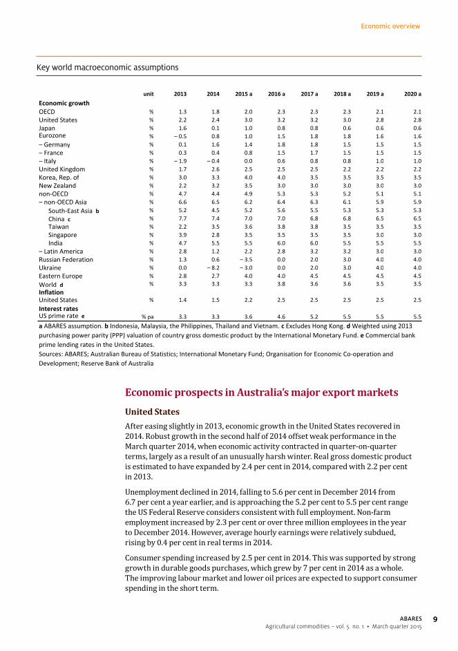
Key world macroeconomic assumptions
unit 2013 2014 2015 a 2016 a 2017 a 2018 a 2019 a 2020 a
OECD % 1.3 1.8 2.0 2.3 2.3 2.3 2.1 2.1United States % 2.2 2.4 3.0 3.2 3.2 3.0 2.8 2.8Japan % 1.6 0.1 1.0 0.8 0.8 0.6 0.6 0.6Eurozone % – 0.5 0.8 1.0 1.5 1.8 1.8 1.6 1.6– Germany % 0.1 1.6 1.4 1.8 1.8 1.5 1.5 1.5– France % 0.3 0.4 0.8 1.5 1.7 1.5 1.5 1.5– Italy % – 1.9 – 0.4 0.0 0.6 0.8 0.8 1.0 1.0United Kingdom % 1.7 2.6 2.5 2.5 2.5 2.2 2.2 2.2Korea, Rep. of % 3.0 3.3 4.0 4.0 3.5 3.5 3.5 3.5New Zealand % 2.2 3.2 3.5 3.0 3.0 3.0 3.0 3.0non‐OECD % 4.7 4.4 4.9 5.3 5.3 5.2 5.1 5.1– non‐OECD Asia % 6.6 6.5 6.2 6.4 6.3 6.1 5.9 5.9 South‐East Asia b % 5.2 4.5 5.2 5.6 5.5 5.3 5.3 5.3 China c % 7.7 7.4 7.0 7.0 6.8 6.8 6.5 6.5 Taiwan % 2.2 3.5 3.6 3.8 3.8 3.5 3.5 3.5 Singapore % 3.9 2.8 3.5 3.5 3.5 3.5 3.0 3.0 India % 4.7 5.5 5.5 6.0 6.0 5.5 5.5 5.5– Latin America % 2.8 1.2 2.2 2.8 3.2 3.2 3.0 3.0Russian Federation % 1.3 0.6 – 3.5 0.0 2.0 3.0 4.0 4.0Ukraine % 0.0 – 8.2 – 3.0 0.0 2.0 3.0 4.0 4.0Eastern Europe % 2.8 2.7 4.0 4.0 4.5 4.5 4.5 4.5World d % 3.3 3.3 3.3 3.8 3.6 3.6 3.5 3.5
United States % 1.4 1.5 2.2 2.5 2.5 2.5 2.5 2.5
US prime rate e % pa 3.3 3.3 3.6 4.6 5.2 5.5 5.5 5.5
a ABARES assumption. b Indonesia, Malaysia, the Philippines, Thailand and Vietnam. c Excludes Hong Kong. d Weighted using 2013 purchasing power parity (PPP) valuation of country gross domestic product by the International Monetary Fund. e Commercial bank prime lending rates in the United States.Sources: ABARES; Australian Bureau of Statistics; International Monetary Fund; Organisation for Economic Co‐operation and Development; Reserve Bank of Australia
Economic growth
Inflation
Interest rates

10
Economic overview
ABARESAgricultural commodities – vol. 5 no. 1 • March quarter 2015
The US economy benefited from reduced fiscal drag in 2014. For 2014 as a whole, government spending decreased by 0.2 per cent, compared with a fall of 2.0 per cent in 2013. It increased in the September quarter 2014, in year-on-year terms, for the first time in four years. US fiscal policy is expected to be neutral or slightly contractionary over the short term.
Activity in the housing market continued to recover in 2014, although at a slower rate than in 2013. This partly reflected an increase in mortgage rates in the second half of 2013. Housing starts increased by 8.8 per cent in 2014 to one million units. This was the highest annual level since 2007, although the rate of increase was slower than the 18.5 per cent increase achieved in 2013. Building permits, a proxy for future construction, increased by 3.5 per cent in 2014, after increasing by 19.4 per cent in 2013. House prices increased by an average of 5.7 per cent year-on-year in the September quarter 2014, down from 12.0 per cent in 2013 and 11.1 per cent in the first half of 2014.
Selected US housing market indicators
Housing starts (annual rate)
’000units
Home price index (Case-Shiller) year-on-year change (right axis)
%
200
400
600
800
1 000
1 200
1 400
–15
–10
–5
0
5
10
15
Dec2014
Dec2013
Dec2012
Dec2011
Dec2010
Dec2009
Dec2008
In response to strengthening economic growth and the improving labour market, the US Federal Reserve ceased its programme of asset purchases in October 2014. However, interest rates are expected to remain low in the short term. The Federal Reserve board stated in December 2014 that it would be appropriate to maintain rates at their current level ‘for a considerable time’. Accommodating monetary policy, together with a slower rate of fiscal consolidation, is expected to support the economy in the short term.
While the recovery is expected to continue, a number of risks to the outlook persist. Weakness in the economies of the main trading partners of the United States will limit external demand. This will be exacerbated by the recent appreciation of the US dollar, which makes US exports relatively more expensive. Low oil prices will have a slightly negative effect on the US economy. Consumers will benefit from lower prices, but some high-cost domestic oil projects have become uneconomic and reduced investment in the domestic oil industry is likely to be a drag on growth.
In preparing this set of agricultural commodity projections, economic growth in the United States is assumed to strengthen to 3.0 per cent in 2015 and to 3.2 per cent in 2016. Over the medium term, economic growth is assumed to ease slightly to average 2.8 per cent in 2019 and 2020.

11
Economic overview
ABARESAgricultural commodities – vol. 5 no. 1 • March quarter 2015
ChinaThe Chinese economy grew by 7.4 per cent in 2014, the lowest annual rate of growth since 1990 and below the government’s target of 7.5 per cent. Economic growth was lower in the second half of 2014 than in the first half; real gross domestic product grew 7.3 per cent year-on-year in the December and September quarters, down from 7.5 per cent in the June quarter.
The real estate sector continued to slow in 2014 and remains a major source of risk in the economy. Real estate investment grew by 10.5 per cent in 2014, down from 19.8 per cent in 2013. Housing prices declined in almost all major cities during 2014.
Industrial indicators were subdued in 2014, reflecting a gradual transition of the economy away from manufacturing. Growth in industrial production was lower in 2014 than in the previous year. Fixed asset investment grew by 15.7 per cent in 2014, compared with 19.6 per cent in 2013. Investment has been particularly weak in the mining and steel manufacturing sectors. These sectors are under pressure from the slowing real estate sector, which is a major consumer of steel.
Confidence in the Chinese economy weakened during 2014. The Westpac MNI China Consumer Sentiment Indicator was down 10 per cent year-on-year in the December quarter, the fourth consecutive quarter of decline. China’s manufacturing purchasing managers’ index (PMI) declined in the December quarter 2014, averaging 50.4 compared with 51.3 in the September quarter. The non-manufacturing PMI averaged 53.9 in the December quarter, a slight reduction from 54.2 in the September quarter. Index values above 50 indicate expansion.
Growth in China’s exports was subdued because of weak external demand from OECD countries. The value of exports was 4.3 per cent higher in 2014, compared with 6.3 per cent in 2013. China’s total imports in 2014 shrank by 0.9 per cent because of weaker domestic demand for manufacturing inputs. As a result, China’s trade surplus expanded to almost US$50 billion in December 2014, 92 per cent higher than a year earlier.
China’s real import and export growth and trade balance
Exports quarterlyyear-on-year growth
%2014US$b
Trade balance (right axis)
Imports quarterlyyear-on-year growth
0
10
20
30
40
50
60
0
10
20
30
40
50
60
Dec2014
Jun2014
Dec2013
Jun2013
Dec2012
Jun2012
Dec2011
Jun2011
Dec2010
Jun2010

12
Economic overview
ABARESAgricultural commodities – vol. 5 no. 1 • March quarter 2015
Both consumer and producer prices were soft in the second half of 2014. The consumer price index in December 2014 was only 1.5 per cent higher than in December 2013, a rate well below the central bank’s target of 3.5 per cent. Producer prices in the December quarter 2014 fell by 2.7 per cent year-on-year.
Inflation rate in China
%
Dec2014
Jun2014
Dec2013
Jun2013
Dec2012
Jun2012
Dec2011
1
2
3
4
5
In late November 2014, the People’s Bank of China lowered interest rates for the first time since July 2012. The lending rate was reduced to 5.6 per cent from 6 per cent and restrictions on home loans and reserve requirements were loosened.
The recent fall in the crude oil price is likely to have a positive effect on China’s growth during 2015 and 2016 because China is a net importer of energy. However, this positive effect will be dampened by a 50 per cent increase in the oil consumption tax, which is designed to prevent cheaper oil from exacerbating air pollution.
Over the medium term, China’s progress in implementing its reform agenda will be a key determinant of growth. Some of the reforms announced in 2013 can be expected to promote growth. These include strengthening farmers’ land rights and relaxing the household registration system, which is an impediment to permanent migration from the countryside to urban areas. If other reforms, such as liberalisation of the financial sector, proceed successfully, medium-term growth prospects can be expected to improve.
In preparing these commodity forecasts, economic growth in China is assumed to be 7 per cent in both 2015 and 2016, before declining gradually to reach 6.5 per cent in 2020.
JapanEconomic activity in Japan was subdued in 2014, growing by around 0.1 per cent year-on-year. The Japanese economy contracted in both the March and September quarters, before recovering to weak growth in the December quarter.
Consumption was brought forward into the first quarter of 2014 to precede an increase in the consumption tax on 1 April, before dropping off sharply after the tax was implemented. Domestic consumption and production recovered very slowly, resulting in weak economic growth in the rest of the year.

13
Economic overview
ABARESAgricultural commodities – vol. 5 no. 1 • March quarter 2015
The Japanese yen depreciated by around 14 per cent against the US dollar in 2014. In January 2015 the currency fell to a low of 120 yen per US dollar for the first time since 2007. A weaker currency is expected to provide support for Japan’s exports in 2015.
Japanese yen exchange rate
yen/US$
60
70
80
90
100
110
Dec2014
Dec2013
Dec2012
Dec2011
Dec2010
Dec2009
Japanese yen per US dollar(inverted axis)
Inflation in Japan remains below the Bank of Japan’s 2 per cent target. While the depreciation of the yen against the US dollar has supported import prices, the recent decline in oil prices has lowered the inflationary impact. Headline inflation in December 2014 was 2.4 per cent year-on-year, but much of this can be attributed to the consumption tax.
Industrial activity has declined gradually since April 2014, and producer expectations are pessimistic for 2015. The December TANKAN survey of industrial producers showed declining profit expectations for 2015, especially for smaller firms.
Japan’s monetary policy was further loosened at the end of October 2014, with the Bank of Japan increasing its monthly purchases of government bonds. Further fiscal stimulus, worth around 3.5 trillion yen, was approved in December 2014. This spending package, together with corporate tax cuts proposed for 2015, seeks to support domestic demand before the next consumption tax increase now planned for April 2017.
The implementation of planned reforms, particularly to improve participation rates and labour productivity, may improve medium-term growth prospects. However, it is uncertain whether these can offset drag created by demographic factors. Economic growth is expected to remain weak over the medium term despite the positive impact of low oil prices.
Economic growth in Japan is assumed to be 1 per cent in 2015 and 0.8 per cent in 2016, before declining to 0.6 per cent in 2020.
EuropeAfter contracting in 2012 and 2013, economic activity in the eurozone is estimated to have increased by 0.8 per cent in 2014. In the United Kingdom, economic activity grew more strongly, by 1.7 per cent in 2013 and 2.6 per cent in 2014.

14
Economic overview
ABARESAgricultural commodities – vol. 5 no. 1 • March quarter 2015
Industrial production is yet to return to pre-global financial crisis levels in most countries. In the December quarter 2014, industrial production remained below 2008 levels by 12 per cent in France, 21 per cent in Italy and 8 per cent in the eurozone as a whole. In the December quarter 2014, the Markit composite purchasing managers’ index for the eurozone showed the slowest rate of expansion in activity since September 2013.
Industrial production—selected European countries
index2010=100
United Kingdom
Italy
EurozoneFrance
Germany
90
100
110
120
130
Dec2014
Dec2013
Dec2012
Dec2011
Dec2010
Dec2009
Dec2008
Dec2007
Low levels of industrial production, together with persistently high unemployment, indicate high levels of underutilised capacity. For the eurozone as a whole, the unemployment rate averaged 11.4 per cent in December 2014, down from 11.8 per cent a year earlier. Unemployment in Italy increased in the second half of 2014. It averaged 13.2 per cent in the December quarter 2014, up from 12.4 per cent in December 2013. Youth unemployment exceeds 40 per cent in Italy, Spain and Greece.
Unemployment rate—selected European countries
%
United KingdomItaly
EurozoneFrance
Germany
2
4
6
8
10
12
14
16
Dec2014
Dec2013
Dec2012
Dec2011
Dec2010

15
Economic overview
ABARESAgricultural commodities – vol. 5 no. 1 • March quarter 2015
Business and consumer sentiment in the eurozone and the United Kingdom strengthened in the first half of 2014, by an average of 14 per cent and 19 per cent year-on-year, respectively, as measured by the European Commission’s Economic Sentiment Indicator. However, economic sentiment declined in the December quarter 2014, with the index falling quarter-on-quarter by 0.2 per cent in the eurozone and 2 per cent in the United Kingdom.
Inflation in the eurozone has remained below the European Central Bank target of 2 per cent, reflecting weak domestic demand. Inflation averaged 0.4 per cent in 2014 and turned negative in December. Consumer prices decreased by 0.2 per cent year-on-year in December 2014. In an attempt to avoid deflation, the European Central Bank announced a large asset purchasing programme in January 2015.
The depreciation of the euro since mid 2014 has supported eurozone exports. In January 2015 the euro averaged US117 cents, compared with an average of US133 cents for 2014 as a whole. The real value of exports of goods and services from the eurozone increased by an average of 3.6 per cent year-on-year in the first nine months of 2014. However, partial data to November 2014 indicate that export growth may have slowed in the final quarter of 2014.
High levels of government debt will remain a concern over the outlook period. The average government debt-to-GDP ratio in the eurozone decreased from 92.7 in the June quarter 2014 to 92.1 in the September quarter. However, in year-on-year terms the debt-to-GDP ratio increased in the September quarter 2014.
Accommodating monetary policy, a weaker euro and lower oil prices are expected to assist European economies in the short term. Economic activity in the eurozone is assumed to expand by 1.0 per cent in 2015 and by 1.5 per cent in 2016. Over the medium term, economic growth is assumed to average 1.7 per cent a year.
Non-OECD AsiaEconomic growth in non-OECD Asia was mixed in 2014. While economic growth in Malaysia was 6.0 per cent in 2014, up from 4.7 per cent in 2013, growth in Singapore was down to 2.8 per cent from 3.9 per cent in 2013.
Lower oil prices are expected to support economic growth because most countries in the region are net energy importers. India, Indonesia and Malaysia have taken advantage of the lower prices to reduce or remove subsidies on petroleum consumption, which may limit the benefit of lower prices to consumers. However, reduction of these subsidies will improve fiscal balance sheets, facilitating public investment in infrastructure and improving medium-term growth prospects. Lower oil prices are also expected to reduce inflationary pressures for most countries in the region in the short term.
In India, economic growth (at market prices) in the September quarter was 6.0 per cent year-on-year, buoyed by growth in the services sector. Consumer price inflation in November was the lowest since 2011 at 4.4 per cent year-on-year, with low oil prices and an expected high level of food production putting downward pressure on prices. Interest rates were cut from 8 per cent to 7.75 per cent in January 2015. Business remains optimistic about the current government’s reform agenda, which includes financial sector liberalisation and privatisation of public infrastructure. Successful implementation of these reforms will improve investor confidence and support economic growth in India.
16
Economic overview
ABARESAgricultural commodities – vol. 5 no. 1 • March quarter 2015
Political turmoil in Thailand, which restricted economic growth in 2014, has largely abated, providing scope for a return to normal conditions. Although recovery has been slow, inflation is low and the central bank has indicated monetary stimulus may be applied if current fiscal stimulus is unsuccessful.
In the Philippines, economic growth is expected to rebound on the back of a recovery in government spending. In Malaysia, a consumption tax to be introduced in April 2015 is likely to affect growth in the short term.
In the medium term, the reduction of market inefficiencies through structural reforms and increased infrastructure investment should improve growth prospects in the region. However, budget deficits remain a constraint in many countries.
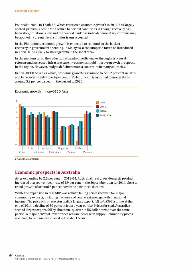
In non–OECD Asia as a whole, economic growth is assumed to be 6.2 per cent in 2015 and to recover slightly to 6.4 per cent in 2016. Growth is assumed to moderate to around 5.9 per cent a year in the period to 2020.
Economic growth in non-OECD Asia
2016a
2015a
2014
2017–20a
%
a ABARES assumption.
1
2
3
4
5
6
7
8
Vietnam
Thailand
Taiwan
Singapore
Philippines
Malaysia
Indonesia
India
China
Economic prospects in AustraliaAfter expanding by 2.5 per cent in 2013–14, Australia’s real gross domestic product increased at a year-on-year rate of 2.9 per cent in the September quarter 2014, close to trend growth of around 3 per cent over the past three decades.
While the expansion in real GDP was robust, falling prices received for major commodity exports, including iron ore and coal, weakened growth in national income. The price of iron ore, Australia’s largest export, fell to US$68 a tonne at the end of 2014, a decline of 50 per cent from a year earlier. Prices for coal, Australia’s second largest export, fell by about one-quarter in US dollar terms over the same period. A major driver of lower prices was an increase in supply. Commodity prices are likely to remain low, at least in the short term.
17
Economic overview
ABARESAgricultural commodities – vol. 5 no. 1 • March quarter 2015
The recent fall in oil prices is expected to have mixed effects on the Australian economy. Lower energy prices will reduce costs in sectors such as manufacturing and agriculture and increase real incomes of households. However, a major negative for the Australian economy is lower revenue from energy exports, especially liquefied natural gas exports (currently Australia’s third-largest export).
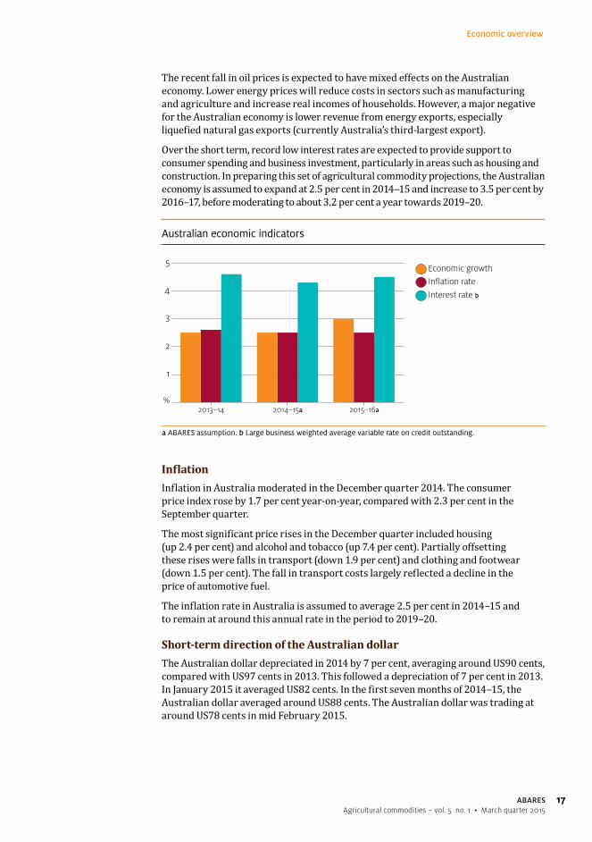
Over the short term, record low interest rates are expected to provide support to consumer spending and business investment, particularly in areas such as housing and construction. In preparing this set of agricultural commodity projections, the Australian economy is assumed to expand at 2.5 per cent in 2014–15 and increase to 3.5 per cent by 2016–17, before moderating to about 3.2 per cent a year towards 2019–20.
Australian economic indicators
%
Economic growth Inflation rate
Interest rate b
a ABARES assumption. b Large business weighted average variable rate on credit outstanding.
1
2
3
4
5
2015–16a2014–15a2013–14
InflationInflation in Australia moderated in the December quarter 2014. The consumer price index rose by 1.7 per cent year-on-year, compared with 2.3 per cent in the September quarter.
The most significant price rises in the December quarter included housing (up 2.4 per cent) and alcohol and tobacco (up 7.4 per cent). Partially offsetting these rises were falls in transport (down 1.9 per cent) and clothing and footwear (down 1.5 per cent). The fall in transport costs largely reflected a decline in the price of automotive fuel.
The inflation rate in Australia is assumed to average 2.5 per cent in 2014–15 and to remain at around this annual rate in the period to 2019–20.
Short-term direction of the Australian dollarThe Australian dollar depreciated in 2014 by 7 per cent, averaging around US90 cents, compared with US97 cents in 2013. This followed a depreciation of 7 per cent in 2013. In January 2015 it averaged US82 cents. In the first seven months of 2014–15, the Australian dollar averaged around US88 cents. The Australian dollar was trading at around US78 cents in mid February 2015.

18
Economic overview
ABARESAgricultural commodities – vol. 5 no. 1 • March quarter 2015
Australian terms of trade and exchange rates
Exchange rate(right axis)
Terms of trade index
20
40
60
80
100
120
140
index2012–13
=100
20
40
60
80
100
120
140
USc/A$
Dec2014
Dec2012
Dec2010
Dec2008
Dec2006
Dec2004
Dec2002
Australia’s terms of trade, the ratio of export prices to import prices, is an indicator of the fundamental value of the Australian dollar. The terms of trade declined by 25 per cent from the September quarter 2011 to the September quarter 2014. This reflects mainly weakening prices on world markets for mineral resources. In the December quarter 2014 the Reserve Bank of Australia commodity price index fell by 21.8 per cent year-on-year in US dollar terms, after falling by 14.7 per cent in the September quarter. The value of the Australian dollar, while volatile, declined by 7.8 per cent against the US dollar and by 3.9 per cent on a trade-weighted basis in the year to the December quarter 2014.
Differentials between interest rates in Australia and major world economies also influence demand for the Australian dollar. Interest rates in Europe, Japan and the United States are substantially lower than in Australia. This encourages international investors to seek higher returns in Australia, thereby maintaining demand for the Australian dollar. Interest rate differentials between Australia and the United States have narrowed in the past year and can be expected to narrow further in the short term, in line with the assumed recovery in the United States and the associated normalisation of US monetary policy. However, the eurozone and Japan both announced large asset purchasing programmes in recent months. Consequently, significant interest rate differentials between Australia and these countries should remain, or even widen, lending support to the Australian dollar.
In addition to these fundamental factors, movements in the Australian dollar are influenced by changes in financial market sentiment towards the Australian economy and by the outlook for major world economies. For example, any indications of stronger than expected growth in the United States, or of weakness in the Australian economy, could lead to reduced investment in Australian assets and result in further depreciation of the Australian dollar.
Any unexpected strengthening or weakening of economic growth in China would affect Australian commodity exports, putting upward or downward pressure on the Australian dollar.

19
Economic overview
ABARESAgricultural commodities – vol. 5 no. 1 • March quarter 2015
Taking these factors into account, the Australian dollar is assumed to average US83 cents and TWI 67 in 2014–15 and US76 cents and TWI 63 in 2015–16. A survey of major Australian commercial banks in early February 2015 indicated varying forecasts for the Australian dollar for the next 12 months. These ranged mostly from around US81 cents to US73 cents. Considerable uncertainty remains in the outlook for the Australian dollar.
Australian dollar assumptions over the medium termAs global economic recovery strengthens over the next few years, the relative attractiveness of foreign assets will increase. However, despite the assumed recovery in OECD countries, growth in the OECD as a whole is expected to be slower than in Australia over the medium term. Yields on Australian securities are also expected to increase once the growth momentum in the Australian economy strengthens and Australian interest rates return to levels closer to their historical averages. Higher interest rate differentials between Australia and major OECD countries should limit downward pressure on the Australian dollar.
As world economic growth recovers over the next few years, demand for Australian commodities is also expected to increase. With relatively strong economic growth assumed in China over the medium term, China’s ongoing demand for Australian commodities is expected to remain strong. This is expected to help support the value of the Australian dollar. Nevertheless, commodity prices can be highly volatile, and this leads to significant uncertainty about the value of the Australian dollar.
In preparing this set of agricultural commodity forecasts, the Australian dollar is assumed to remain at around US76 cents between 2015–16 and 2019–20, close to its 30-year average.
Key macroeconomic assumptions for Australia
unit 2012–13 2013–14 2014–15 a 2015–16 a 2016–17 a 2017–18 a 2018–19 a 2019–20 aunit 2012 13 2013 14 2014 15 a 2015 16 a 2016 17 a 2017 18 a 2018 19 a 2019 20 aEconomic growth % 2 5 2 5 2 5 3 0 3 5 3 5 3 2 3 2Economic growth % 2.5 2.5 2.5 3.0 3.5 3.5 3.2 3.2flInflation % 2.3 2.6 2.5 2.5 2.5 2.5 2.5 2.5
Interest rates b % pa 5.2 4.6 4.3 4.5 5.5 6.0 6.0 6.0Interest rates b % pa 5.2 4.6 4.3 4.5 5.5 6.0 6.0 6.0Nominal exchange ratesUS$/A$ US$ 1 03 0 92 0 83 0 76 0 76 0 76 0 76 0 76
Nominal exchange rates– US$/A$ US$ 1.03 0.92 0.83 0.76 0.76 0.76 0.76 0.76Trade‐weighted index
for A$ c index 77 71 67 63 63 62 62 62Trade weighted index for A$ c index 77 71 67 63 63 62 62 62a ABARES assumption b Large business weighted average variable rate on credit outstanding c Base: May 1970 100a ABARES assumption. b Large business weighted average variable rate on credit outstanding. c Base: May 1970 = 100.Sources: ABARES; Australian Bureau of Statistics; Reserve Bank of Australia; ;

20
Economic overview
ABARESAgricultural commodities – vol. 5 no. 1 • March quarter 2015
Outlook for Australian agricultural and fisheries exportsThe total volume of farm production is forecast to decrease by 0.9 per cent in 2015–16, following a forecast decline of 4.6 per cent in 2014–15. The forecast decline in 2014–15 reflects expected falls in crop production from a record high in 2013–14. Farm production is projected to rise gradually over the medium term, reaching 2013–14 levels again by 2019–20, under the assumption of favourable seasonal conditions.
The index of unit returns for Australian farm exports is forecast to increase by 4.2 per cent in 2015–16, following a forecast rise of 3.0 per cent in 2014–15. An assumed weaker Australian dollar is expected to increase the average export price for agricultural products in Australian dollar terms. For wheat and sugar, the assumed depreciation of the Australian dollar in 2015–16 is expected to more than offset weaker world prices in US dollar terms. Higher export prices in 2015–16 are also expected for beef, wool, wine, canola and dairy products. Towards 2019–20, unit returns for farm exports are projected to decline gradually, in real terms.
Earnings from farm exports are forecast to increase by 0.6 per cent in 2015–16 to around $40.5 billion, following a forecast fall of 2.1 per cent to $40.3 billion in 2014–15. Increases in farm export earnings in 2015–16 are forecast for wheat (up 12 per cent), sugar (11 per cent), canola (10 per cent), dairy products (8 per cent) and beef and veal (2 per cent). However, this is expected to be largely offset by declines in export earnings for mutton (down 39 per cent), cotton (35 per cent), barley (11 per cent) and lamb (8 per cent).
Export earnings from crops are forecast to increase by 2.9 per cent in 2015–16 to around $21.0 billion, compared with a forecast fall of 10.7 per cent in 2014–15 to $20.4 billion. The export value of livestock and livestock products is forecast to decrease by 1.8 per cent in 2015–16 to $19.5 billion, following an expected increase of 8.5 per cent to $19.9 billion in 2014–15.
At the end of the projection period (2019–20), the value of Australian farm exports is projected to be around $41.2 billion (in 2014–15 dollars), around 9 per cent higher than the five-year average to 2013–14 of $37.6 billion (also in 2014–15 dollars).
For fisheries products, export earnings are forecast to increase by 8 per cent in 2015–16 to around $1.5 billion. Export earnings in 2015–16 are forecast to rise by 11 per cent for rock lobster and by 9 per cent for tuna and frozen prawns. The value of Australian fisheries exports is projected to be around $1.4 billion (in 2014–15 dollars) in 2019–20.
In December 2014 the Korea–Australia Free Trade Agreement entered into force, followed by the Japan–Australia Economic Partnership Agreement in January 2015. It is anticipated that the China–Australia Free Trade Agreement will enter into force in late 2015. Over the outlook period the three agreements will improve Australia’s competitiveness in these markets for a range of agricultural exports.

21
Economic overview
ABARESAgricultural commodities – vol. 5 no. 1 • March quarter 2015
Major indicators of Australia’s agriculture and natural resources based sectors
2012–13 2013–14 2014–15 f 2015–16 f 2016–17 z 2017–18 z 2018–19 z 2019–20 zExchange rate US$/A$ 1.03 0.92 0.83 0.76 0.76 0.76 0.76 0.76
Farm index 90.2 97.0 100.0 104.2 106.8 109.2 110.4 110.5– real b index 95.0 99.4 100.0 101.7 101.7 101.4 100.0 97.6
Farm A$m 38 019 41 150 40 270 40 507 42 000 43 699 45 251 46 599– real b A$m 40 011 42 162 40 270 39 519 39 976 40 579 40 995 41 187Crops A$m 23 063 22 813 20 378 20 970 21 906 22 834 23 727 24 439– real b A$m 24 271 23 374 20 378 20 458 20 851 21 203 21 496 21 600Livestock A$m 14 956 18 337 19 892 19 537 20 094 20 865 21 523 22 160– real b A$m 15 740 18 788 19 892 19 061 19 125 19 376 19 499 19 586Fisheries products A$m 1 175 1 304 1 347 1 456 1 499 1 529 1 560 1 591– real b A$m 1 237 1 336 1 347 1 420 1 427 1 420 1 413 1 406
Farm A$m 48 501 53 149 51 631 54 380 56 515 58 766 60 719 62 558– real b A$m 51 042 54 456 51 631 53 054 53 792 54 570 55 009 55 292Crops A$m 28 394 30 001 27 116 28 490 29 560 30 705 31 541 32 295– real b A$m 29 881 30 739 27 116 27 795 28 136 28 513 28 574 28 544Livestock A$m 20 107 23 148 24 515 25 890 26 955 28 061 29 179 30 263– real b A$m 21 161 23 717 24 515 25 259 25 656 26 057 26 435 26 748Fisheries products A$m 2 381 2 555 2 577 2 688 2 781 2 843 2 947 3 016– real b A$m 2 506 2 617 2 577 2 622 2 647 2 640 2 670 2 666Forestry products A$m 1 520 1 799 1 857 1 908 1 957 2 005 2 053 2 136– real b A$m 1 600 1 843 1 857 1 861 1 862 1 862 1 860 1 888
Farm index 119.5 126.1 120.2 119.2 120.1 122.2 124.2 126.7– crops index 133.0 139.7 126.6 129.0 131.4 134.2 136.3 138.4– livestock index 104.7 111.1 112.2 108.1 107.8 109.2 111.0 113.9Forestry index 107.9 120.1 123.3 125.3 127.5 129.7 132.1 134.6
grains and oilseeds ’000 ha 23 841 23 567 23 728 23 939 23 999 24 119 24 260 24 389Forestry plantation area ’000 ha 2 013 na na na na na na naSheep million 75.5 72.7 70.7 72.1 73.2 74.2 75.2 76.1Cattle million 29.3 28.5 27.0 26.5 26.6 27.0 27.3 27.2
Net cash income e A$m 16 265 20 101 18 927 20 446 20 076 20 134 20 487 20 933– real b A$m 17 117 20 595 18 927 19 947 19 108 18 696 18 560 18 502Net value of farm production g A$m 11 066 14 759 13 443 14 814 14 293 14 196 14 390 14 673– real b A$m 11 646 15 122 13 443 14 453 13 604 13 183 13 037 12 969Farmers’ terms of trade h index 95.3 98.4 100.3 105.1 103.0 101.9 101.5 100.7
MajorindicatorsofAustralia'sagricultureandnaturalresourcebasedsectors
Australian export unit returns a
Gross value of production c
Volume of production d
a Base: 2014–15 = 100. b In 2014–15 Australian dollars. c For a definition of the gross value of farm production see Table 13. d Chain‐weighted basis using Fisher’s ideal index with a reference year of 1997–98 = 100. e Gross value of farm production less increase in assets held by marketing authorities and less total cash costs. f ABARES forecast. g Gross value of farm production less total farm costs. h Ratio of index of prices received by farmers and index of prices paid by farmers, with a reference year of 1997–98 = 100. z ABARES projection. na Not available.Sources: ABARES; Australian Bureau of Statistics; Reserve Bank of Australia
Value of exports
Production area and livestock numbersCrop area
Farm sector

22
Economic overview
ABARESAgricultural commodities – vol. 5 no. 1 • March quarter 2015
Major Australian agricultural commodity exports a
WorldpriceValue ValueVolume
2015–16
2014–15f
2015–16f
$b
a Wheat, cotton, sugar, canola, cheese, skim milk powder and whole milk powder are world indicator prices in US$. All other commodities are export unit returns or domestic prices in A$. f ABARES forecast.
Mutton
Skim milk powder
Rock lobster
Live feeder/slaughter cattle
Cheese
Cotton
Canola
Lamb
Sugar
Barley
Wine
Wool
Wheat
Beef and veal2%
12%
0%
4%
–11%
11%
–8%
10%
–35%
9%
–5%
11%
16%
–39%
–5%
6%
–4%
–1%
–7%
7%
–10%
2%
–34%
1%
–10%
3%
3%
–37%
16%
–2%
3%
5%
–4%
–2%
2%
3%
–14%
6%
6%
8%
9%
–3%
$8.01b
$5.43b
$2.71b
$1.78b
$2.04b
$1.53b
$1.64b
$1.25b
$1.55b
$0.75b
$0.85b
$0.58b
$0.49b
$0.80b
$8.14b
$6.07b
$2.72b
$1.84b
$1.81b
$1.70b
$1.50b
$1.37b
$1.00b
$0.81b
$0.81b
$0.64b
$0.57b
$0.49b
2 4 6 8 10

23
Economic overview
ABARESAgricultural commodities – vol. 5 no. 1 • March quarter 2015
Key agricultural outcomes of recent free trade agreementsMatthew Hyde
Since 2013 the Australian Government has concluded free trade agreement (FTA) negotiations with the Republic of Korea, Japan and China. These agreements will reduce or eliminate import tariffs on many Australian agricultural exports to these countries over the next 20 years.
This article discusses the key agricultural outcomes of the China–Australia Free Trade Agreement (ChAFTA) and summarises the Korea–Australia Free Trade Agreement (KAFTA) and the Japan–Australia Economic Partnership Agreement (JAEPA).
Key agricultural outcomes of the China–Australia Free Trade Agreement
On 17 November 2014 the Australian and Chinese governments concluded negotiations for ChAFTA. China has been Australia’s largest export market for agricultural commodities since 2010–11, averaging around 19 per cent of total agricultural exports in the four years to 2013–14, worth around $6.8 billion. It is anticipated that the agreement will enter into force by late 2015.
In 2013 Australia supplied 8 per cent of China’s US$112 billion agricultural imports (excluding seafood) and was the third-largest individual supplier behind the United States (23 per cent) and Brazil (20 per cent). In 2013 Australia was the principal supplier to China of barley (74 per cent), wool (69 per cent) and beef (57 per cent).
Under ChAFTA, China’s import tariffs on many Australian agricultural exports—including dairy products, beef, sheep meat, hides and skins, livestock, seafood, wine and horticulture—are to be removed over periods of up to 11 years. Most products will be tariff free within four years, while tariffs on some grains, including grain sorghum and barley, will be eliminated when the agreement enters into force. For wool, Australia will obtain exclusive access to a tariff-free quota that will start at 30 000 tonnes clean equivalent and grow to almost 45 000 tonnes over eight years. Australia will retain access to China’s multilateral wool tariff-rate quota (TRQ), which has an in-quota tariff of 1 per cent.
Australia’s exports of wheat, rice, cotton, sugar, canola and vegetable oils receive no tariff concessions or additional market access under ChAFTA. However, tariff concessions on imports of these products have been excluded from all China’s existing FTAs. China’s wheat and rice imports are currently subject to a 1 per cent tariff under the existing multilateral TRQs, which are rarely filled because China is a major world producer of both grains. China also imports cotton and sugar under multilateral TRQs, although the quotas for these commodities are often binding and over-quota tariff rates are applied. Imports of canola and vegetable oils face tariffs of up to 25 per cent.
continued ...

24
Economic overview
ABARESAgricultural commodities – vol. 5 no. 1 • March quarter 2015
Key agricultural outcomes of recent free trade agreements continued
Key agricultural outcomes under the China–Australia Free Trade Agreement
Commodity Outcome
Milk powders Removal of 10 per cent tariff on skim and whole milk powders
over 11 years, with a safeguard measure on imports of whole
milk powder.
Cheese Removal of 15 per cent tariff on blue vein cheeses over four years
and 12 per cent tariff on all other cheeses over nine years.
Fluid milk Removal of 15 per cent tariff over nine years.
Other dairy products Removal of 15 per cent tariff on infant formula over four years.
Removal of tariffs between 10 per cent and 19 per cent on
ice-cream, lactose, casein and milk albumins over four years.
Removal of 10 per cent tariff on butter and yoghurt over nine years.
Beef Removal of tariffs between 12 per cent and 25 per cent on beef
within nine years, with a safeguard measure.
Removal of 12 per cent tariff on beef offal over seven years.
Sheep meat Removal of tariffs between 12 per cent and 23 per cent over
eight years.
Wool Creation of a tariff-free quota for Australian wool. The quota will
commence at 30 000 tonnes (clean equivalent) and grow by
5 per cent a year over eight years.
Sheep and bovine
hides and skins
Removal of tariffs between 5 per cent and 14 per cent over
seven years.
Live animals Removal of tariffs up to 10 per cent over four years.
Pig meat Removal of tariffs up to 20 per cent over four years.
Seafood Removal of tariffs between 10 per cent and 15 per cent on all
seafood (excluding sharkfin), including the 14 per cent tariff on
abalone and the 15 per cent tariff on rock lobster, over four years.
Wine Removal of 20 per cent tariff on bulk wine and 14 per cent tariff
on bottled wine over four years.
Horticulture Removal of all tariffs on horticulture, including tariffs up to
25 per cent on nuts over four years and tariffs up to 30 per cent
on citrus over eight years.
Grains Removal of 3 per cent tariff on barley and 2 per cent tariff on
grain sorghum on commencement of the agreement.
Source: Australian Department of Foreign Affairs and Trade 2015, ‘China–Australia Free Trade Agreement. Fact sheet: agriculture and processed food’, available at dfat.gov.au/trade/agreements/chafta/fact-sheets/Pages/fact-sheet-agriculture-and-processed-food.aspx
continued ...

25
Economic overview
ABARESAgricultural commodities – vol. 5 no. 1 • March quarter 2015
Key agricultural outcomes of recent free trade agreements continued
Safeguard measures
Under ChAFTA, China will have the option to impose specific safeguard measures on imports of beef and whole milk powder from Australia. These measures are designed to protect the Chinese industry from injury caused by significant increases in imports over a short period. Safeguard measures can be applied if the volume of product imported from Australia exceeds an annual threshold. If applied, the import tariff will be restored to the most-favoured nation (MFN) applied tariff rate for the remainder of the calendar year.
Under ChAFTA, the beef safeguard threshold starts at 170 000 tonnes, which is about 10 per cent higher than China’s imports of Australian beef in 2013. China will increase the threshold by 3 per cent a year over the first 10 years of the agreement. Australia will also face a discretionary safeguard on whole milk powders. The safeguard trigger volume will start at 17 500 tonnes and increase by 5 per cent a year—well above current and past trade levels. Both safeguards have an automatic review to allow their removal if Australian trade is found not to be causing injury to the Chinese industry.
China’s existing free trade agreements
At the start of 2015, China had nine FTAs in effect, covering trade with 17 countries. China commenced agreements with the ASEAN countries in 2005, Chile in 2006, Iceland and Pakistan in 2007, New Zealand in 2008, Singapore in 2009, Peru in 2010, Costa Rica in 2011 and Switzerland in 2014.
Compared with China’s other FTAs, the agricultural outcomes achieved by Australia in ChAFTA have shorter tariff elimination time frames for some products (such as nuts and some other horticultural products) and fewer safeguards.
China–Australia Free Trade Agreement outcomes for Australian agricultural commodities
Dairy
In 2013 China imported US$7.2 billion of dairy products, representing a 900 per cent increase over the previous decade in real terms. Australia supplied around 4 per cent of that total, down from 10 per cent a decade earlier. Australia’s market share was lost mainly to New Zealand—the dominant supplier of dairy products to China—which had an import share of around 51 per cent by value in 2013.
New Zealand is the only major dairy exporter with an existing free trade agreement with China. China’s imports of New Zealand dairy are dominated by milk powders, which are scheduled to be tariff free in 2019. Assuming ChAFTA comes into force in 2015, China’s imports of Australian milk powders will be subject to a tariff of 5 per cent in 2019. Australian exports of milk powder to China will be tariff free in 2026.
Under ChAFTA, a dairy-specific safeguard measure (to be reviewed in 15 years) is imposed only on imports of Australian whole milk powder. This compares with the imposition of separate safeguard measures on imports of many New Zealand dairy products. The safeguard measures in the New Zealand–China Free Trade Agreement (NZ–China FTA) apply to imports of fluid milk, milk powders, cheese and butter.
continued ...

26
Economic overview
ABARESAgricultural commodities – vol. 5 no. 1 • March quarter 2015
Key agricultural outcomes of recent free trade agreements continued
The annual safeguard volume for milk powder has been exceeded by New Zealand every year since 2009. In 2013 the annual threshold volume was breached as early as 28 January. Under the specific safeguard measures, the MFN tariff rate of 10 per cent has been applied to imports of New Zealand milk powder for the remainder of each calendar year.
China dairy imports by source
2013US$b
Other
Australia
United States
Source: United Nations Commodity Trade Statistics Database (UN Comtrade)
1
2
3
4
5
6
7
8
European Union
New Zealand
20132011200920072005
Beef
China’s total beef imports were US$1.3 billion in 2013, almost 400 per cent higher than the previous year. Australia was the major beneficiary of the strong import growth after China banned beef imports from Brazil and the United States because of concerns over bovine spongiform encephalopathy. An agreement to allow imports of Brazilian beef was signed in November 2014, although no official trade has been recorded at time of publication.
China beef imports by source
2013US$m
Other
New Zealand
Uruguay
Source: United Nations Commodity Trade Statistics Database (UN Comtrade)
Australia
20132012201120102009
200
400
600
800
1 000
1 200
1 400
continued ...
27
Economic overview
ABARESAgricultural commodities – vol. 5 no. 1 • March quarter 2015
Key agricultural outcomes of recent free trade agreements continued
Under ChAFTA, all import tariffs on Australian beef will be removed within nine years, which is a similar time frame to that agreed to under the NZ–China FTA. Imports of Australian beef will be subject to a specific safeguard measure, while New Zealand beef is not. By 2016 China’s imports of New Zealand beef are scheduled to be tariff free. Assuming ChAFTA comes into force in 2015, Australian beef will be tariff free in China by 2024.
China applies different import tariff rates and export establishment registration requirements according to the type of beef imported. Almost 80 per cent of China’s imports of Australian beef were frozen cuts in 2013, which are subject to a tariff rate of 12 per cent, compared with a tariff of 25 per cent on carcasses. Imports of chilled beef ceased in September 2013 as a result of Chinese registration requirements. However, shipments of chilled beef imports from Australia recommenced in July 2014, after the Chinese Government approved 10 Australian establishments to commence chilled beef exports on a trial basis.
Wool and sheep meat
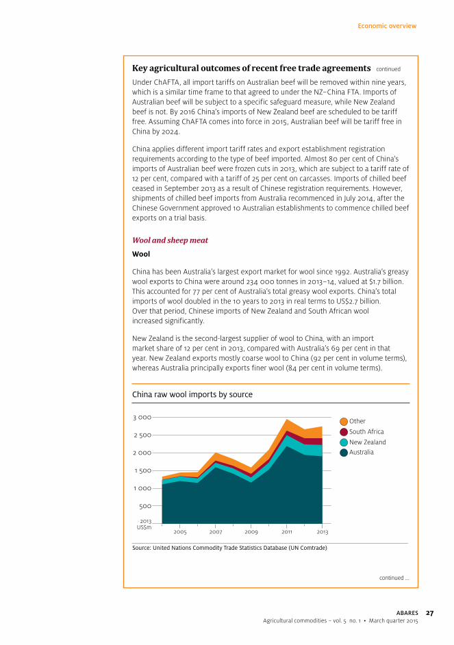
Wool
China has been Australia’s largest export market for wool since 1992. Australia’s greasy wool exports to China were around 234 000 tonnes in 2013–14, valued at $1.7 billion. This accounted for 77 per cent of Australia’s total greasy wool exports. China’s total imports of wool doubled in the 10 years to 2013 in real terms to US$2.7 billion. Over that period, Chinese imports of New Zealand and South African wool increased significantly.
New Zealand is the second-largest supplier of wool to China, with an import market share of 12 per cent in 2013, compared with Australia’s 69 per cent in that year. New Zealand exports mostly coarse wool to China (92 per cent in volume terms), whereas Australia principally exports finer wool (84 per cent in volume terms).
China raw wool imports by source
2013US$m
Other
South Africa
New Zealand
Source: United Nations Commodity Trade Statistics Database (UN Comtrade)
Australia
20132011200920072005
500
1 000
1 500
2 000
2 500
3 000
continued ...

28
Economic overview
ABARESAgricultural commodities – vol. 5 no. 1 • March quarter 2015
Key agricultural outcomes of recent free trade agreements continued
China’s wool imports are managed through a multilateral TRQ set at 287 000 tonnes, with a 1 per cent in-quota tariff and a 38 per cent out-of-quota tariff. Although China’s wool imports usually exceed the quota, the out-of-quota rate has not been applied by the Chinese Government in the past three years.
Under ChAFTA, Australia gains access to an additional tariff-free wool quota. When ChAFTA enters into force, the volume of the quota will be 30 000 tonnes clean equivalent (or 43 000 tonnes greasy). Australia will also retain access to the multilateral TRQ.
Sheep meat
Australia and New Zealand are the two dominant suppliers of sheep meat to China, with New Zealand supplying 57 per cent of China’s imported sheep meat and Australia supplying 39 per cent. Although China’s overall imports of sheep meat increased 17-fold in the decade ending 2013, import market shares between Australia and New Zealand have remained largely unchanged. In 2013–14 Australian sheep meat exports to China totalled $393 million, accounting for around 18 per cent of Australia’s overall sheep meat exports.
Under ChAFTA, China’s imports of Australian sheep meat will be tariff free in eight years, the same time frame achieved in the NZ–China FTA. Sheep meat imports from New Zealand will be tariff free in 2016. Assuming ChAFTA comes into force in 2015, Australian sheep meat imports will be tariff free in 2023.
Wine
The value of China’s table wine imports increased 23-fold in the decade to 2013 in real terms, reaching US$1.5 billion. In that year, Australia supplied 16 per cent of China’s table wine imports. Its main competitors are the European Union (which exports high quality bottled wine) and Chile (which typically exports lower quality bulk wine). Other smaller volume competitors include the United States, Argentina and New Zealand.
In China, premium bottled table wines dominate the import market, as opposed to lower value bulk wine. The share of imported bottled table wine, by value, grew from 51 per cent in 2004 to 93 per cent in 2013. Almost all China’s imports of Australian wine in that year were of bottled table wine.
China table wine imports by source
2013US$m
Other
United States
Chile
Note: Table wines do not include sparkling or fortfied wines.Source: United Nations Commodity Trade Statistics Database (UN Comtrade)
Australia
20132011200920072005
European Union
500
1 000
1 500
2 000
continued ...

29
Economic overview
ABARESAgricultural commodities – vol. 5 no. 1 • March quarter 2015
Key agricultural outcomes of recent free trade agreements continued
Of the many countries that export a significant volume of wine to China, only Chile and New Zealand have an FTA with China. Since the implementation of the Chile–China Free Trade Agreement in 2006, the import value of Chilean wine in China grew almost sevenfold in real terms in the period to 2013. The import value of New Zealand bottled wine also increased significantly between 2008 and 2013, although from a low base.
Under ChAFTA, imports of Australian wine will be tariff free after four years. This will provide the same preference currently enjoyed by Chile and New Zealand and a competitive advantage for Australian wine imports against imports from the European Union and the United States, Australia’s principal competitors in the bottled wine segment of China’s import market. Countries without an FTA with China will continue to face the MFN import tariffs of 20 per cent on bulk wine and 14 per cent on bottled wine.
Horticulture
The value of Australian horticultural exports to China was around $82 million in 2013–14. Most of these exports were fruit and tree nuts, which each totalled $37 million. Citrus fruit comprised the largest share of fruit exported and China was the third-largest export market for Australian citrus fruit in that year. Macadamia nuts comprised the largest share of the export value of tree nuts to China.
Under ChAFTA, China’s imports of Australian nuts and table grapes will be tariff free after four years, while imports of citrus fruit will be tariff free within eight years. None of Australia’s major competitors in China’s citrus fruit or macadamia nut import market have an FTA with China.
Table grapes are China’s second-largest fruit import, valued at US$515 million in 2013. Chile and Peru compete with Australia in China’s table grapes market and both countries have FTAs with China. After implementation of the Chile–China Free Trade Agreement in 2006 and the Peru–China Free Trade Agreement in 2010, China’s imports of table grapes from Chile increased by 448 per cent and from Peru by 384 per cent, by value, in the period to 2013. The two countries now dominate the market, with import shares of 45 per cent for Chile and 19 per cent for Peru, by value, in 2013. Their products were tariff free in China as of 1 January 2015.
Key agricultural outcomes of the Japan–Australia Economic Partnership Agreement
On 15 January 2015 the Japan–Australia Economic Partnership Agreement (JAEPA) came into force. Under JAEPA, Australian exports of beef, cheese, wine, horticulture, seafood, vegetable oils, livestock, pork, honey, wheat and feed barley have preferential tariff access to Japan.
Tariff cuts under JAEPA occur on 1 April each year. Australia received its first cuts when JAEPA entered into force on 15 January 2015 and will receive its second round of tariff cuts and quota increases on 1 April 2015. This means tariff cuts and quota increases have been further frontloaded.
continued ...

30
Economic overview
ABARESAgricultural commodities – vol. 5 no. 1 • March quarter 2015
Key agricultural outcomes of recent free trade agreements continued
Japan currently has 14 economic partnership agreements in force, including an agreement with the ASEAN countries. Of these, only Mexico and Australia have achieved preferential access for beef, Australia’s largest agricultural export to Japan.
Under JAEPA, Australia is now the only country that can export feed wheat and feed barley to Japan without participating in a complex quota system. Australia now also has exclusive access to TRQs for cheese, pork and other products.
Key agricultural outcomes under the Japan–Australia Economic Partnership Agreement
Commodity Outcome
Beef The 38.5 per cent tariff on frozen beef was reduced to 30.5 per cent
on commencement of the agreement. It will be cut by a further
2 percentage points in the second year and 1 percentage point in the
third year, before declining evenly to 19.5 per cent by 1 April 2031.
The 38.5 per cent tariff on chilled beef was reduced to 32.5 per cent on
commencement of the agreement. It will be cut by 1 percentage point a
year for the following two years, before declining evenly to 23.5 per cent
by 1 April 2028.
Japan’s 50 per cent global snapback tariff will no longer apply to imports
of Australian beef and will be replaced by a discretionary safeguard.
Reduction of duties on preserved and prepared beef and beef offal.
Australia will also receive access to growing duty-free TRQs for
these products.
Dairy Creation of a bilateral duty-free TRQ for imports of Australian
unprocessed cheese, which started at 4 000 tonnes on commencement
of the agreement. The quota limit will increase by 1 000 tonnes on
1 April 2015 and evenly thereafter to 20 000 tonnes on 1 April 2034.
Creation of preferential TRQs for other types of cheese imported from
Australia, including grated and powdered cheese, processed cheese
and unprocessed cheese for making shredded cheese, with quota limits
increasing for the first 10 years of the agreement.
Grains Exports of feed barley and feed wheat to Japan will be tariff free and
outside the multilateral TRQ system. Special safeguard measures will no
longer apply to imports of Australian feed barley and feed wheat.
Creation of a large Australia-only duty-free TRQ for unroasted malt.
In the first year of the agreement, Australia will be able to export
8 600 tonnes duty free (assessed pro-rata because the first year
extends only from 15 January 2015 to 31 May 2015), with the quota
limit growing to 86 000 tonnes by 1 April 2024.
continued ...

31
Economic overview
ABARESAgricultural commodities – vol. 5 no. 1 • March quarter 2015
Key agricultural outcomes of recent free trade agreements continued
Key agricultural outcomes of the Korea–Australia Free Trade Agreement
On 12 December 2014 the Korea–Australia Free Trade Agreement (KAFTA) entered into force. Under KAFTA, tariffs are to be eliminated on a wide range of agricultural commodities, including beef, wheat, sugar, wine and seafood.
Sugar The 21.5 yen/kilogram tariff on high polarity raw sugar was
eliminated and the domestic levy was reduced on commencement
of the agreement.
Oilseeds
and oilsThe 3.5 per cent tariff on fish liver oil and the 7 per cent tariff on other
fish oil were eliminated on commencement of the agreement. Tariffs of
between 10.9 yen/kilogram and 13.2 yen/kilogram on canola oil and
8.5 yen/kilogram on cottonseed oil will be removed in equal stages by
1 April 2024.
Horticulture The 3 per cent tariffs on asparagus and many vegetables and 5 per cent
tariff on macadamia nuts were eliminated on commencement of
the agreement.
The 16 per cent tariff on oranges will be removed through equal annual
reductions by 1 April 2024 (for oranges imported between 1 June and
30 September).
Removal of tariffs of up to 34 per cent on most fresh and canned fruit
and vegetables over periods of up to 15 years.
Wine Removal of the 15 per cent or specific tariff of 82 yen/litre for sparkling
wine and up to 125 yen/litre for wine in two-litre containers through
equal annual reductions by 1 April 2021. Removal of tariffs of up to
125 yen/litre for wine containers of up to 150 litres by 1 April 2024.
Wine in containers larger than 150 litres became duty free on
commencement of the agreement.
Seafood Tariffs of up to 5 per cent for prawns and rock lobster and up to
7 per cent for abalone were eliminated on commencement of the
agreement. Tariffs of 3.5 per cent on southern bluefin tuna and
salmon are to be removed by 1 April 2024.
Pig meat A preferential TRQ for Australia was established on commencement of
the agreement, starting at 5 600 tonnes and rising evenly to 14 000 by
1 April 2019. Japan’s safeguard measures on pig meat imports will no
longer apply to imports from Australia.
Source: Australian Department of Foreign Affairs and Trade 2014, ‘Japan–Australia Economic Partnership Agreement. Fact sheet: agriculture and processed food’, available at dfat.gov.au/trade/agreements/jaepa/fact-sheets/Pages/fact-sheet-agriculture-and-processed-food.aspx
continued ...

32
Economic overview
ABARESAgricultural commodities – vol. 5 no. 1 • March quarter 2015
Key agricultural outcomes of recent free trade agreements continued
Tariff cuts under KAFTA occur on 1 January each year. Australia received its first cuts when the agreement entered into force on 15 December 2014 and received its second round of tariff cuts and quota increases on 1 January 2015.
The main beneficiaries of the agreement are expected to be exporters of beef, cheese, malting barley and malt, which are currently subject to relatively high import tariffs. For a more detailed analysis of the agricultural outcomes of KAFTA, see ‘Korea–Australia Free Trade Agreement’ (ABARES 2014).
Key agricultural outcomes under the Korea–Australia Free Trade Agreement
Commodity Outcome
Beef Removal of 40 per cent tariff on beef and 18 per cent tariff on
bovine offal by 2028.
Phasing out of import tariffs on edible offal, including from bovine
animals, from the current applied rate of 18 per cent. The 72 per cent
tariff on processed beef products will also be phased out.
Sugar The 3 per cent tariff on raw sugar was locked in at zero on
commencement of the agreement. Korea has in recent years
unilaterally applied a 0 per cent tariff.
Removal of 35 per cent tariff on refined sugar through equal
annual reductions by 2031.
Cheese Immediate duty-free quota, which started at 4 630 tonnes and
grows until out-of-quota tariffs on cheeses listed in this table
are eliminated:
– Cheddar cheese Removal of 36 per cent tariff through equal annual reductions
by 2026.
– Grated and
powdered cheese
and speciality
cheeses
Removal of 36 per cent tariff through equal annual reductions
by 2033.
– Mozzarella, cream
cheese, processed
cheese and all
other cheeses
Removal of 36 per cent tariff through equal annual reductions
by 2031.
Butter Removal of 89 per cent tariff through equal annual reductions by
2028. Over this period, Australia will receive access to a tariff-free
quota. The quota started at 113 tonnes, is now 115 tonnes and
increases to 146 tonnes by the end of the tariff phase-out period.
After 2028 Australia will have unlimited duty-free access.
Sheep and goat meat Removal of 22.5 per cent tariff on sheep and goat meat through
equal annual reductions by 2023.
Pig meat Removal of 22.5 per cent tariff on fresh pig meat by 2028 and
25 per cent tariff on some frozen pig meat by 2018.
continued ...

33
Economic overview
ABARESAgricultural commodities – vol. 5 no. 1 • March quarter 2015
Key agricultural outcomes of recent free trade agreements continued
References
ABARES 2014, Agricultural commodities, June quarter 2014, vol. 4, no. 2, Australian Bureau of Agricultural and Resource Economics and Sciences, Canberra.
Wine The 15 per cent tariff on wine was eliminated on commencement
of the agreement.
Horticulture The 24 per cent tariff on cherries, 8 per cent tariff on almonds
and 21 per cent tariff on dried grapes were eliminated on
commencement of the agreement.
Removal of tariffs ranging from 27 per cent to 54 per cent
on products such as macadamia nuts, fruit juices, mangoes,
asparagus and lentils over three to 10 years.
Elimination of tariffs during Australia’s exporting seasons on
potatoes for chipping (Australia’s largest horticultural export with
current tariff of up to 304 per cent) effective immediately.
Phasing out of the 50 per cent tariff on oranges, 24 per cent tariff
on fresh table grapes and 144 per cent tariff on mandarins.
Wheat The 1.8 per cent to 3 per cent tariff on wheat was eliminated on
commencement of the agreement.
Malt and malting
barley
Immediate and growing duty-free quota for malt and malting barley
and elimination of out-of-quota tariffs of 269 per cent on malt and
513 per cent on malting barley over 15 years by 2028.
During that period, Australia will have access to a single tariff-free
quota across both goods. The quota started at 10 000 tonnes
and will increase to almost 13 000 tonnes by the end of the tariff
phase-out period.
Oilseeds The 3 per cent tariff on cottonseed was eliminated on
commencement of the agreement, and the 8 per cent and
10 per cent tariffs on canola oil products will be eliminated
through equal annual reductions by 2023.
Seafood Key products, such as frozen southern bluefin tuna (current
tariff of 10 per cent) and rock lobster (20 per cent) will enter the
Republic of Korea duty free by 2016.
Source: Australian Department of Foreign Affairs and Trade 2014, ‘Korea–Australia Free Trade Agreement. Fact sheet: trade in goods’, available at dfat.gov.au/trade/agreements/kafta/fact-sheets/Pages/fact-sheet-trade-in-goods.aspx

34
Economic overview
ABARESAgricultural commodities – vol. 5 no. 1 • March quarter 2015
Effect of a depreciation of the Australian dollar on farm sector earningsOver the past several months the value of the Australian dollar has declined markedly against the US dollar. Between September 2014 and February 2015, the Australian dollar depreciated from an average of around US94 cents to around US77 cents. This compares with a high of around US103 cents averaged over 2012–13.
The US dollar has also strengthened against other major currencies in recent months. The US dollar traded at around 77 euro cents, 62 pence sterling and 106 yen in early September 2014, compared with 88 euro cents, 66 pence sterling and 119 yen in mid February 2015. Over the same period, the US dollar appreciated by around 13 per cent against a basket of major floating international currencies.
Recent movements in the US dollar, monthly
index A$/US$
Major �oating currency index
Australian dollar, inverted (right axis)
Sources: ABARES; Reserve Bank of Australia; US Federal Reserve
65
70
75
80
85
90
0.8
0.9
1.0
1.1
1.2
1.3
Jan2015
Jul2014
Jan2014
Jul2013
Jan2013
Jul2012
Jan2012
The depreciation of the Australian dollar against the US dollar is expected to have a positive impact on farm performance and incomes. Close to 65 per cent of Australia’s agricultural production is exported and export contracts are mostly denominated in US dollar terms, so a decline in the value of the Australian dollar against the US dollar is expected to increase export earnings. Partially offsetting this gain will be upward pressure on prices of imported inputs (including fertiliser, machinery and fuel), which will cost more in Australian dollars. However, the net effect on the farm sector is likely to be positive.
The effect of a depreciation of the Australian dollar on farm sector earnings is estimated here under three main assumptions. The first is that around 60 per cent of the depreciation of the Australian dollar is a result of a rise in the value of the US dollar. The second is that a 15 per cent rise in the US dollar will result in a 4 per cent decline in aggregate world agricultural prices in US dollar terms. This is because an appreciation of the US dollar is similar to a reduction in the purchasing power of commodity importing countries (all else being equal), resulting in weaker demand and lower prices. The third is that there is no supply response to changes in export prices or export earnings. See ABARE (2009) for details of the analyses supporting these assumptions.
continued ...

35
Economic overview
ABARESAgricultural commodities – vol. 5 no. 1 • March quarter 2015
Effect of a depreciation of the Australian dollar on farm sector earnings continued
Using the ABARES forecast of farm export earnings of $40.3 billion in 2014–15 and the assumed exchange rate of US83 cents, a further depreciation of the Australian dollar by US1 cent is estimated to directly increase the value of farm exports by around $490 million (all other factors remaining equal).
Partially offsetting the estimated increase in the value of farm exports would be a decline in world agricultural prices in US dollar terms. Assuming that around 60 per cent of the depreciation of the Australian dollar is a result of a strengthening US dollar, a fall of US1 cent in the Australian dollar would result in lower world prices and reduce Australian farm export earnings by around 16 per cent. This would reduce the gain in farm sector earnings to around $410 million.
In addition, a lower Australian dollar would put upward pressure on the price of imported farm inputs, which are estimated to account for around 20 per cent of total farm costs. Using the ABARES forecast of farm costs of around $38.2 billion in 2014–15, a US1 cent depreciation of the Australian dollar would raise farm costs by around $90 million (assuming importers, wholesalers and retailers passed on price increases in full to farmers). The net effect would be an increase in farm sector incomes of around $320 million.
This estimate is somewhat higher than the net effect of $200 million presented in ABARE (2009). This estimated larger effect on farm sector incomes mainly reflects the higher value of farm exports forecast for 2014–15 (at $40.3 billion). The value of farm exports was around $27.8 billion in 2009–10.
ReferencesABARE 2009, Australian commodities: December quarter 2009, Australian Bureau of Agricultural and Resource Economics, Canberra.

36
Economic overview
ABARESAgricultural commodities – vol. 5 no. 1 • March quarter 2015
Seasonal conditions in AustraliaMatthew Miller and Dean Mansfield
Recent rainfall and cooler than normal seasonal conditions throughout much of central and eastern Australia have benefited pasture growth and crop production and replenished on-farm water supplies. In response to the improved seasonal conditions, livestock producers have been active at both store and physical markets in New South Wales, Victoria and Queensland in an attempt to secure young cattle, lambs and breeders for herd and flock rebuilding. Grains producers have responded to improved seasonal conditions by increasing summer crop plantings, especially for grain sorghum.
Rainfall percentiles, Australia, 3 months to January 2015
Source: Bureau of Meteorology, issued 3 February 2015
90–100 Extremely high
Rainfall percentiles
70–80 Above average
80–90 Well above average
30–70 Average
Wheat–sheep zone
10–20 Well below average20–30 Below average
5–10 Extremely low0–5 Severe de�ciency
South Australia
NorthernTerritory
Western Australia
Queensland
New SouthWales
Victoria
Australian CapitalTerritory
Tasmania
Despite recent improvement in seasonal conditions, severe rainfall deficiencies for the 18 months to January 2015 remained across parts of Queensland, New South Wales, South Australia, Victoria and Western Australia, although the area affected in Queensland and New South Wales contracted markedly. Despite this, around two-thirds of Queensland remains drought declared. The Queensland Government has identified 44 shires as fully drought declared and a further three shires as partially drought declared. In New South Wales, the area most affected by low rainfall is the north-east of the state. In Victoria, dry conditions are centred on the Wimmera and Mallee districts, while in South Australia rainfall deficiencies have been most severe in the south-east of the state.
continued ...

37
Economic overview
ABARESAgricultural commodities – vol. 5 no. 1 • March quarter 2015
Seasonal conditions in Australia continued
Rainfall percentiles, Australia, 18 months to January 2015
Source: Bureau of Meteorology, issued 3 February 2015
90–100 Extremely high
Rainfall percentiles
70–80 Above average
80–90 Well above average
30–70 Average
Wheat–sheep zone
10–20 Well below average20–30 Below average
5–10 Extremely low0–5 Severe de�ciency
South Australia
NorthernTerritory
Western Australia
Queensland
New SouthWales
Victoria
Australian CapitalTerritory
Tasmania
Relative levels of modelled upper layer soil moisture (~0.2 metres) and lower layer soil moisture (~0.2 to ~1.5 metres) across Australia for January 2015. The bulk of plant roots are in the top 0.3 metres of the soil profile. Soil moisture in the upper layer of the soil profile (0.2 metres) is therefore the most appropriate indication of the availability of water, particularly for germinating plants. Upper layer soil moisture responds quickly to seasonal conditions and will often show a pattern that reflects rainfall and temperature events of the same month. The lower layer soil moisture is a larger, deeper store that is slower to respond to rainfall and tends to reflect accumulated events over longer periods. Crops and pastures can draw on this deeper soil moisture store once they have become established and when needed to support production, throughout the growing season.
Relative upper layer soil moisture for January 2015 was predominantly above average to extremely high across much of eastern, northern and central Australia. In Western Australia, relative upper layer soil moisture was variable, ranging from extremely low in the south to extremely high in the north. Across summer cropping regions in Queensland and northern New South Wales, relative upper layer soil moisture was predominantly well above average. This pattern of relative upper layer soil moisture reflects rainfall received to the end of January 2015.
Relative lower layer soil moisture for January 2015 was predominantly above average to extremely high across much of northern and central Australia. Across the central Queensland cropping region, relative lower layer soil moisture was largely average to above average, with largely below average to extremely low relative lower layer soil moisture in southern Queensland and northern New South Wales cropping regions. Across southern New South Wales, Victoria and Western Australia relative lower layer soil moisture was variable, although levels tend towards below average. In contrast, relative lower layer soil moisture levels remain above average across much of South Australia.
continued ...

38
Economic overview
ABARESAgricultural commodities – vol. 5 no. 1 • March quarter 2015
Seasonal conditions in Australia continued
Upper layer soil moisture, January 2015
Source: Australian Water Availability Project (ABARES; Bureau of Meteorology; CSIRO)
South Australia
NorthernTerritory
Western Australia
Queensland
New SouthWales
Victoria
Tasmania
Relative soil moisturepercentiles
0–1010–2020–3030–4040–5050–6060–7070–8080–9090–100
Australian CapitalTerritory
Wheat–sheep zone
Lower layer soil moisture, January 2015
Note: Soil moisture estimates are relative to the long-term record and ranked in percentiles. The data presented in these maps compare the upper and lower layer soil moisture from January 2015and ranks it according to the percentiles of all Januarys in the standard climatological 1961 to1990 reference period. The areas of 0th to 10th percentiles indicate where estimated soil moisture levelsfor January 2015 fell into the three lowest Januarys in the 30-year reference period.Source: Australian Water Availability Project (ABARES; Bureau of Meteorology; CSIRO)
South Australia
NorthernTerritory
Western Australia
Queensland
New SouthWales
Victoria
Tasmania
Relative soil moisturepercentiles
0–1010–2020–3030–4040–5050–6060–7070–8080–9090–100
Australian CapitalTerritory
Wheat–sheep zone
continued ...

39
Economic overview
ABARESAgricultural commodities – vol. 5 no. 1 • March quarter 2015
Seasonal conditions in Australia continued
The Bureau of Meteorology’s latest seasonal rainfall outlook (February to April 2015), issued on 29 January 2015, indicates an increased chance of drier than normal conditions across much of Australia. For cropping areas, chances of exceeding the median rainfall are between 35 per cent and 45 per cent.
While recent rainfall has raised upper layer soil moisture levels, seasonal conditions over the next several months will be critical for winter crop planting for the 2015–16 season. Without sufficient rainfall across a number of key growing regions in eastern Australia, the area planted to winter crops in these regions could be adversely affected. Similarly, insufficient rainfall would also affect herd and flock rebuilding by livestock producers.
Australian rainfall outlook, February to April 2015
Sources: Bureau of Meteorology, issued 29 January 2015
South Australia
NorthernTerritory
Western Australia
Queensland
New SouthWales
Victoria
Tasmania
Australian CapitalTerritory
Chance of exceedingthe median rainfall (%)
80%75%70%65%60%55%50%45%40%35%30%25%20%
Wheat–sheep zone

40
Economic overview
ABARESAgricultural commodities – vol. 5 no. 1 • March quarter 2015

41
Economic overview
ABARESAgricultural commodities – vol. 5 no. 1 • March quarter 2015
AgricultureCrops

42 ABARESAgricultural commodities – vol. 5 no. 1 • March quarter 2015
Grains and oilseedsOutlook to 2019–20
Clay Mifsud, David Mobsby and Christopher Price
• In 2015–16 the world indicator price for corn is forecast to increase, while the world indicator prices for wheat and soybeans are forecast to fall.
• World indicator prices for grains and oilseeds are projected to average lower in real terms over the period to 2019–20, compared with the five years to 2014–15.
• World corn production is forecast to fall in 2015–16, reflecting a decline in area planted coinciding with an increase in area planted to soybeans.
• Growth in grains and oilseeds production over the medium term is expected to be concentrated in relatively low cost producing regions, including the Black Sea region and Latin America.
• Australian grains and oilseeds production is projected to rise over the outlook period and is expected to support an increase in export volumes.
World outlook for 2015–16Prices
WheatThe world wheat indicator price (US no. 2 hard red winter, fob Gulf) is forecast to average US$265 a tonne in 2015–16, compared with US$270 a tonne in 2014–15. Assuming average seasonal conditions in 2015–16, an increase in the supply of high-quality milling wheat is expected despite an overall decline in world wheat production. In the previous year, there were low supplies of milling grade wheat (including hard red winter wheat) in the United States and harvest quality issues in other major wheat producing countries. A risk to the price forecast is the uncertainty around the condition of the northern hemisphere winter wheat crop, which will soon emerge from dormancy.
Coarse grainsThe world coarse grains indicator price (US no. 2 yellow corn, fob Gulf) is forecast to increase by 8 per cent in 2015–16 to average US$193 a tonne. This reflects an expected increase in demand for corn and a forecast decline in production from the record achieved in 2014–15. The world barley indicator price (France feed barley, fob Rouen) is forecast to increase by 9 per cent in 2015–16 to average US$226 a tonne.
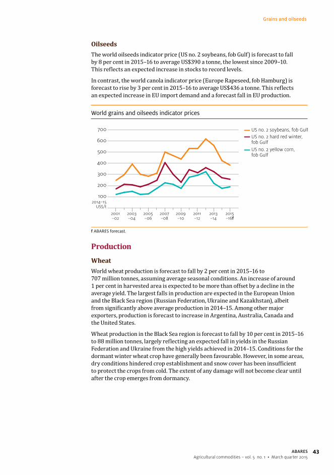
43
Grains and oilseeds
ABARESAgricultural commodities – vol. 5 no. 1 • March quarter 2015
OilseedsThe world oilseeds indicator price (US no. 2 soybeans, fob Gulf) is forecast to fall by 8 per cent in 2015–16 to average US$390 a tonne, the lowest since 2009–10. This reflects an expected increase in stocks to record levels.
In contrast, the world canola indicator price (Europe Rapeseed, fob Hamburg) is forecast to rise by 3 per cent in 2015–16 to average US$436 a tonne. This reflects an expected increase in EU import demand and a forecast fall in EU production.
World grains and oilseeds indicator prices
2014–15US$/t
US no. 2 soybeans, fob GulfUS no. 2 hard red winter,fob GulfUS no. 2 yellow corn,fob Gulf
100
200
300
400
500
600
700
f ABARES forecast.
2015–16f
2013–14
2011–12
2009–10
2007–08
2005–06
2003–04
2001–02
Production
WheatWorld wheat production is forecast to fall by 2 per cent in 2015–16 to 707 million tonnes, assuming average seasonal conditions. An increase of around 1 per cent in harvested area is expected to be more than offset by a decline in the average yield. The largest falls in production are expected in the European Union and the Black Sea region (Russian Federation, Ukraine and Kazakhstan), albeit from significantly above average production in 2014–15. Among other major exporters, production is forecast to increase in Argentina, Australia, Canada and the United States.
Wheat production in the Black Sea region is forecast to fall by 10 per cent in 2015–16 to 88 million tonnes, largely reflecting an expected fall in yields in the Russian Federation and Ukraine from the high yields achieved in 2014–15. Conditions for the dormant winter wheat crop have generally been favourable. However, in some areas, dry conditions hindered crop establishment and snow cover has been insufficient to protect the crops from cold. The extent of any damage will not become clear until after the crop emerges from dormancy.

44
Grains and oilseeds
ABARESAgricultural commodities – vol. 5 no. 1 • March quarter 2015
Forecast change in world wheat production, 2015–16
Volume change
Percentage change(right axis)
Mt %
–10
–5
0
5
10
–10
–5
0
5
10
rest ofworld
United StatesBlack Searegion
EuropeanUnion
In the European Union, wheat production is forecast to fall by 8 per cent in 2015–16 to 143 million tonnes. The forecast decline largely reflects an expected fall in yields following high yields across much of the European Union in the previous year. Overall, crop quality is expected to be better than the previous year, when heavy rainfall during harvest adversely affected quality in some regions.
Wheat production in the United States is forecast to increase by 6 per cent in 2015–16 to 58 million tonnes. This forecast increase follows production declines in the past two years. Harvested area is forecast to increase by 1 per cent and the average yield is expected to rise by 4 per cent. Planted area of winter wheat is estimated to have declined by 5 per cent, including a 3 per cent fall in area planted to hard red winter wheat. However, harvested area is expected to increase because of an assumed fall in the winter wheat abandonment rate to around the 10-year average.
Coarse grainsWorld production of coarse grains is forecast to fall by 2 per cent in 2015–16 to 1.25 billion tonnes, largely reflecting an expected decline in world corn production. Following record production in 2014–15, world corn production is forecast to fall by 3 per cent in 2015–16 to 965 million tonnes, reflecting expected falls in planted area and yields, particularly in the United States. Production is also expected to decline in the European Union and the Black Sea region. Small increases are expected in China and Latin America.
In the United States, corn production is forecast to fall by 7 per cent in 2015–16 to 345 million tonnes. The area planted to corn is forecast to fall by 4 per cent to 32 million hectares, reflecting more favourable returns from soybean production. The average yield is assumed to fall by 3 per cent in 2015–16 from the record high achieved in 2014–15.

45
Grains and oilseeds
ABARESAgricultural commodities – vol. 5 no. 1 • March quarter 2015
World coarse grains production
Commodity2013–14
Mt2014–15f
Mt2015–16f
Mt
Corn 989 990 965
Barley 145 139 138
Other 146 144 145
Total 1 280 1 273 1 248
f ABARES forecast.
Corn production in the European Union is forecast to fall by 11 per cent in 2015–16 to 65 million tonnes, reflecting an expected fall in planted area and an assumed return to average yields from the record high achieved in 2014–15. The area planted to corn is forecast to fall by 6 per cent to 9.3 million hectares because of an expected decline in returns from corn production relative to other grains.
In the major Latin American exporting countries (Argentina and Brazil), corn production is forecast to increase by 3 per cent in 2015–16 to 101 million tonnes, driven by an expected increase in area planted. Corn production is forecast to increase by 2 per cent in Brazil to 77 million tonnes and by 4 per cent in Argentina to 24 million tonnes.
World barley production is forecast to fall by 1 per cent in 2015–16 to 138 million tonnes, largely reflecting a decline from the above average yields achieved in 2014–15. Lower production in the European Union and the Black Sea region is forecast to more than offset higher production in North America.
World barley production
2013–14
Mt
2014–15f
2015–16f
rest ofworld
Australia
LatinAmerica
North America
Black Searegion
EuropeanUnion
10
20
30
40
50
60
10
20
30
40
50
60
f ABARES forecast.

46
Grains and oilseeds
ABARESAgricultural commodities – vol. 5 no. 1 • March quarter 2015
OilseedsWorld oilseeds production is forecast to fall by 2 per cent in 2015–16 to 522 million tonnes. World soybean production is forecast to fall by 2 per cent to 307 million tonnes and world canola production is forecast to fall by 4 per cent to 69 million tonnes. In contrast, world production of sunflower seed is forecast to rise.
In the United States, soybean production is forecast to fall by 4 per cent to 104 million tonnes, driven by an assumed decline in yields from the above average yields achieved last year. However, producers are forecast to increase the area planted to soybeans. Despite the forecast fall in the soybean indicator price in 2015–16, returns from planting soybeans are expected to remain more favourable in the United States than the returns from planting corn.
In Latin America, the area planted to soybeans in 2015–16 is forecast to be largely unchanged from the previous season. Assuming a return to trend yields, soybean production is forecast to rise by 1 per cent in Brazil to 95 million tonnes but fall by less than 1 per cent in Argentina to 55 million tonnes.
World soybean production and area
Production
MhaMt
Harvested area(right axis)
f ABARES forecast.
150
100
50
200
250
300
350
20
40
60
80
100
120
140
2015–16f
2012–13
2009–10
2006–07
2003–04
2000–01
1997–98
1994–95
1991–92
CanolaWorld canola production is forecast to decline by 4 per cent in 2015–16 to 69 million tonnes. This forecast reflects expected falls in production in the European Union and Ukraine more than offsetting a forecast production increase in Canada.
EU rapeseed (canola) production is forecast to decline by 14 per cent to 20.6 million tonnes. The area planted to winter rapeseed (which account for more than 90 per cent of total EU rapeseed area) is estimated to have fallen by 6 per cent in 2015–16.
Rapeseed (canola) production in Ukraine is forecast to fall by 22 per cent in 2015–16 to 1.7 million tonnes. The area planted to winter rapeseed, which typically accounts for more than 90 per cent of total rapeseed area, is estimated to have fallen by around 5 per cent.
Canola production in Canada is forecast to rise by 3 per cent in 2015–16 to 16 million tonnes, reflecting a 3 per cent increase in area planted. The area planted is forecast to increase because of relatively favourable returns expected from canola.

47
Grains and oilseeds
ABARESAgricultural commodities – vol. 5 no. 1 • March quarter 2015
Consumption
WheatWorld consumption of wheat is forecast to decline by 1 per cent in 2015–16 to 707 million tonnes, which largely reflects an expected 5 per cent decline in the use of wheat for feed. This reflects expected reductions in wheat consumption in the European Union and the Black Sea region from 2014–15, when there were abundant regional supplies of feed wheat. The use of wheat for human consumption, which accounts for around 70 per cent of total consumption, is forecast to increase by 1 per cent but mainly reflects population growth.
Coarse grainsWorld coarse grains consumption is forecast to increase by 1 per cent in 2015–16 to 1.26 billion tonnes. Consumption of corn is forecast to increase, because of higher feed and industrial use. Consumption of barley and other coarse grains is forecast to be largely unchanged from 2014–15.
World coarse grains consumption
Commodity2013–14
Mt2014–15f
Mt2015–16f
Mt
Corn
Feed 576 595 605
Food, seed and industrial uses 370 373 375
Barley
Feed 97 94 95
Food, seed and industrial uses 42 43 43
f ABARES forecast.
World corn consumption is forecast to increase by 1 per cent in 2015–16 to a record of 980 million tonnes. This reflects a 2 per cent increase in the use of corn as feed to 605 million tonnes and a 1 per cent increase in the use of corn for industrial purposes to 375 million tonnes. Total corn consumption is forecast to rise in the United States, China and Latin America.
Corn consumption in the United States is forecast to rise by 1 per cent in 2015–16 to 305 million tonnes, driven by an expected increase in the demand for feed. The industrial use of corn, which is mostly for ethanol production, is forecast to be largely unchanged in 2015–16 at around 169 million tonnes.
World barley consumption is forecast to increase by 1 per cent in 2015–16, to 138 million tonnes.

48
Grains and oilseeds
ABARESAgricultural commodities – vol. 5 no. 1 • March quarter 2015
OilseedsTotal oilseeds consumption is forecast to rise by 2 per cent in 2015–16 to 514 million tonnes.
World oilseeds crush is forecast to rise by 2 per cent in 2015–16 to 451 million tonnes, driven by strong world demand for protein meals and vegetable oil. World protein meal production is forecast to rise by 3 per cent to 300 million tonnes and vegetable oil production is forecast to rise by 3 per cent to 180 million tonnes.
World use of vegetable oil is forecast to grow by 1 per cent in 2015–16 to 179 million tonnes. Food consumption of vegetable oil is expected to rise by around 1 per cent to 133 million tonnes and industrial consumption of vegetable oil is forecast to rise by 1 per cent to 45 million tonnes. This growth is slower than previous years, which reflects an expected slowdown in biodiesel production in Argentina.
World protein meal use is forecast to rise by 3 per cent in 2015–16 to 297 million tonnes. Soybean meal consumption is forecast to rise by 4 per cent to 205 million tonnes, with large consumption increases expected in China and Brazil.
Trade
WheatWorld trade in wheat is forecast to fall by 3 per cent in 2015–16 to 147 million tonnes, despite expected strong import demand for milling grade wheat. Exports from the United States are expected to increase by 13 per cent in 2015–16 but this is expected to be more than offset by declines in exports from other major exporters, including Canada, the European Union and the Black Sea region.
Coarse grainsWorld trade in coarse grains is forecast to increase by 1 per cent in 2015–16 to 152 million tonnes. World trade in corn is forecast to increase by 2 per cent in 2015–16 to 117 million tonnes, reflecting an expected increase in imports into the European Union, Mexico and Japan. World trade in barley and other coarse grains is forecast to fall slightly.
Corn imports into the European Union are forecast to increase by 13 per cent in 2015–16 to 9 million tonnes, primarily reflecting two factors. First, the supply of feed wheat is expected to be significantly lower than the previous year when a high proportion of the wheat crop was graded as feed. Second, corn production in the European Union is forecast to decline in 2015–16 and more imports will be required to satisfy the demand for feed.
Corn imports into Mexico are forecast to increase by 4 per cent in 2015–16 to 11.3 million tonnes, reflecting expected higher feed demand. Over the coming year, pig meat, poultry and dairy production are forecast to increase by between 1 per cent and 3 per cent. Most of this forecast increase in corn imports is expected to be sourced from the United States. Over the five years to 2014–15, more than 90 per cent of corn imports into Mexico were from the United States.

49
Grains and oilseeds
ABARESAgricultural commodities – vol. 5 no. 1 • March quarter 2015
Corn imports, European Union
Mt
f ABARES forecast.
5
10
15
20
2015–16f
2012–13
2009–10
2006–07
2003–04
2000–01
Imports of corn into China are forecast to remain largely unchanged in 2015–16. In December 2014 China’s Ministry of Agriculture lifted a ban on the importation of MIR162, a GM variety of corn grown in the United States, Argentina and Brazil. The ban was in place from December 2013. During this period imports of non-GM feed grains, including barley and grain sorghum, increased.
World trade in barley is forecast to fall by 3 per cent in 2015–16 to 21 million tonnes, reflecting an expected fall of imports into China. The Chinese Government’s decision to permit imports of the genetically modified corn variety MIR162 is likely to result in lower imports of barley. Imports of feed barley are likely to be replaced by imports of distiller’s dried grain, a by-product of corn-based ethanol production. Demand for barley in the other major import markets, Saudi Arabia and Japan, is expected to be largely unchanged in the short term. Growth in demand for livestock feed is expected to be met by imports of other feed grains.
OilseedsWorld oilseeds exports are forecast to rise by 2 per cent in 2015–16 to 136 million tonnes. World soybean exports are forecast to increase by 1.5 per cent to 116 million tonnes, driven by a forecast increase in imports into China. Exports are forecast to rise by 16 per cent from Argentina to 9.5 million tonnes and by 4 per cent from Brazil to 48 million tonnes. US soybean exports are forecast to decline by 6 per cent to 46 million tonnes because an expected rise in US soybean crush is expected to limit the supply of soybeans available for export.
World canola trade is forecast to rise by 4 per cent in 2015–16 to 14 million tonnes, largely reflecting an expected increase in canola imports into the European Union. This follows below average EU imports expected in 2014–15 because of above average production in that year. Canola exports from Canada are expected to rise. Most of the forecast exports from Canada are expected to go to the United States, Mexico, China and Japan, so the most of the expected increase in EU imports is forecast to be met by shipments from Australia and Ukraine.

50
Grains and oilseeds
ABARESAgricultural commodities – vol. 5 no. 1 • March quarter 2015
World oilseeds trade
Mt
Other
Canola Soybeans
20
40
60
80
100
120
140
160
2015–16f
2012–13
2009–10
2006–07
2003–04
2000–01
1997–98
1994–95
1991–92
f ABARES forecast.
Stocks
WheatWorld closing stocks of wheat are expected to be largely unchanged in 2015–16 at around 192 million tonnes. The combined stocks of the major exporting countries are forecast to decline but remain well above the lows of 2007–08 and 2012–13.
World wheat closing stocks
Rest of world
Major exporters a
Mt %
Stocks-to-use ratio(right axis)
10
20
30
40
50
a Argentina, Australia, the Black Sea region, Canada, the European Union and the United States. f ABARES forecast.
50
100
150
200
250
2015–16f
2012–13
2009–10
2006–07
2003–04
2000–01
1997–98

51
Grains and oilseeds
ABARESAgricultural commodities – vol. 5 no. 1 • March quarter 2015
Coarse grainsWorld coarse grains stocks are forecast to fall by 7 per cent in 2015–16 to 214 million tonnes, primarily reflecting a decline in corn stocks. Corn consumption is forecast to exceed production for the first time in three years and stocks are expected to fall by 6 per cent in 2015–16 to 182 million tonnes. The largest declines in stocks are expected to be in the United States and Latin America. Corn stocks are forecast to fall by 12 per cent in the United States to 46 million tonnes and by 14 per cent in Latin America to 18 million tonnes.
World barley stocks are forecast to fall by 5 per cent in 2015–16 to 22 million tonnes. The largest decline in stocks is expected in the Russian Federation, with a forecast fall of 27 per cent to 1.6 million tonnes.
OilseedsWorld closing stocks of oilseeds are forecast to rise by 7 per cent in 2015–16 to a record 113 million tonnes. Although world oilseeds production is forecast to fall, it is still expected to exceed world consumption by around 8 million tonnes. World soybean stocks are forecast to increase to 102 million tonnes, with stocks expected to increase in the three major exporting countries, Argentina, Brazil and the United States. In contrast, world canola stocks are forecast to decline to around 5 million tonnes, largely reflecting an expected run-down in stocks in the European Union in response to expected falls in domestic production.
World oilseeds closing stocks
Mt
Soybeans Canola Other
2015–16f
2012–13
2009–10
2006–07
2003–04
2000–01
1997–98
1994–95
1991–92
f ABARES forecast.
20
40
60
80
100
120
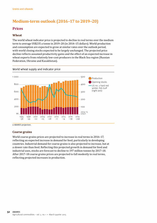
52
Grains and oilseeds
ABARESAgricultural commodities – vol. 5 no. 1 • March quarter 2015
Medium-term outlook (2016–17 to 2019–20)Prices
WheatThe world wheat indicator price is projected to decline in real terms over the medium term to average US$235 a tonne in 2019–20 (in 2014–15 dollars). World production and consumption are expected to grow at similar rates over the outlook period, with world closing stocks expected to be largely unchanged. The projected price decline reflects assumed productivity gains and the effect of an expected increase in wheat exports from relatively low-cost producers in the Black Sea region (Russian Federation, Ukraine and Kazakhstan).
World wheat supply and indicator price
Production
Opening stocks
Mt2014–15US$/t
US no. 2 hard red winter, fob Gulf (right axis)
200
400
600
800
1 000
100
200
300
400
500
z ABARES projection.
2019–20z
2016–17z
2013–14
2010–11
2007–08
2004–05
2001–02
1998–99
1995–96
Coarse grainsWorld coarse grains prices are projected to increase in real terms in 2016–17, reflecting an expected increase in demand for feed, particularly in developing countries. Industrial demand for coarse grains is also projected to increase, but at a slower rate than feed. Reflecting this projected growth in demand for feed and industrial uses, stocks are forecast to decline to 197 million tonnes by 2017–18. After 2017–18 coarse grains prices are projected to fall modestly in real terms, reflecting projected increases in production.
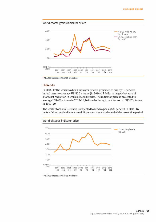
53
Grains and oilseeds
ABARESAgricultural commodities – vol. 5 no. 1 • March quarter 2015
World coarse grains indicator prices
2014–15US$/t
France feed barley, fob RouenUS no. 2 yellow corn, fob Gulf
400
300
200
100
f ABARES forecast. z ABARES projection.
2019–20z
2017–18z
2015–16f
2013–14
2011–12
2009–10
2007–08
2005–06
2003–04
2001–02
OilseedsIn 2016–17 the world soybean indicator price is projected to rise by 10 per cent in real terms to average US$420 a tonne (in 2014–15 dollars), largely because of a forecast reduction in world oilseeds stocks. The indicator price is projected to average US$421 a tonne in 2017–18, before declining in real terms to US$387 a tonne in 2019–20.
The world stocks-to-use ratio is expected to reach a peak of 22 per cent in 2015–16, before falling gradually to around 19 per cent towards the end of the projection period.
World oilseeds indicator price
2014–15US$/t
US no. 2 soybeans, fob Gulf
f ABARES forecast. z ABARES projection.
2019–20z
2017–18z
2015–16f
2013–14
2011–12
2009–10
2007–08
2005–06
2003–04
2001–02
100
200
300
400
500
600
700

54
Grains and oilseeds
ABARESAgricultural commodities – vol. 5 no. 1 • March quarter 2015
Consumption
WheatWorld wheat consumption is projected to rise by an average of around 1 per cent a year from 2015–16 to 732 million tonnes in 2019–20. Use of wheat for human consumption is projected to increase in line with population growth over the medium term to reach 508 million tonnes in 2019–20. The use of wheat for feed is projected to rise, but the increase is likely to be constrained by competition from alternative feed sources. The use of wheat for industrial purposes is also projected to rise, but is expected to grow slowly and remain a relatively small proportion of total wheat consumption.
World wheat consumption
Mt
FoodFeedOther
z ABARES projection.
100
200
300
400
500
600
700
800
2019–20z
2016–17z
2013–14
2010–11
2007–08
2004–05
2001–02
1998–99
1995–96
Coarse grains World coarse grains consumption is projected to increase at an average annual rate of 1 per cent over the projection period to reach 1.3 billion tonnes in 2019–20, led by an expected increase in the use of coarse grains for feed.
World coarse grains consumption
Food, seed and industrial
Feed
Mt
300
600
900
1200
1 500
z ABARES projection.
2016–17z
2019–20z
2013–14
2010–11
2007–08
2004–05
2001–02
1998–99
1995–96

55
Grains and oilseeds
ABARESAgricultural commodities – vol. 5 no. 1 • March quarter 2015
The use of coarse grains for feed is projected to increase by an average of 2 per cent a year to 806 million tonnes in 2019–20. Income growth in emerging market economies is expected to result in increasing consumption of livestock products, resulting in increased demand for feed.
Growth in the use of coarse grains for industrial purposes is projected to slow and average less than 1 per cent a year to 2019–20. Over the 10 years to 2014–15, the use of coarse grains for industrial purposes grew at an average annual rate of 4 per cent, largely because of the rapid increase in US ethanol production. Over the medium term, little growth is expected in the use of corn for ethanol production in the United States because of limits stipulated in the Renewable Fuel Standard. Other industrial uses such as malting and starch are projected to increase in line with world population growth.
Vegetable oil and protein mealWorld use of vegetable oil and protein meal are both expected to rise by 3 per cent a year to 203 million tonnes and 332 million tonnes, respectively. This demand is underpinned by growth in world population and incomes.
World vegetable oil use is expected to be driven mainly by higher food use. The food use of vegetable oil is projected to rise by 2.8 per cent a year to 154 million tonnes in 2019–20. Per person consumption of vegetable oil for food is projected to rise by 2 per cent a year to 20.1 kilograms in 2019–20.
World vegetable oil consumption
Mt
Food consumptionIndustrial consumption
160
120
80
40
z ABARES projection.
2019–20z
2016–17z
2013–14
2010–11
2007–08
2004–05
2001–02
1998–99
1995–96
World protein meal use is expected to be driven by growth in world livestock production. Soybean meal use is projected to rise by 3 per cent a year to 234 million tonnes in 2019–20, which is expected to be driven by an average annual increase of 5 per cent in the use of soybean meal in China. By 2019–20 the use of soybean meal is expected to have grown to 71 million tonnes.
US soybean meal use is projected to rise by 1 per cent a year to around 30 million tonnes in 2019–20. The projected increase is expected to be driven principally by growth in livestock production.

56
Grains and oilseeds
ABARESAgricultural commodities – vol. 5 no. 1 • March quarter 2015
US soybean meal consumption
Mt
40
30
20
10
z ABARES projection.
2019–20z
2016–17z
2013–14
2010–11
2007–08
2004–05
2001–02
1998–99
1995–96
Oilseeds crushWorld oilseeds crush is projected to increase by 2.5 per cent a year to 486 million tonnes by 2019–20. Soybean crush is expected to account for two-thirds of the expected increase in world oilseeds crush. Soybean crush in China is projected to rise by 4 per cent a year to 92 million tonnes by 2019–20, reflecting growing demand from domestic livestock producers.
World oilseeds crush
Mt
100
200
300
400
500
z ABARES projection.
2019–20z
2016–17z
2013–14
2010–11
2007–08
2004–05
2001–02
1998–99
1995–96

57
Grains and oilseeds
ABARESAgricultural commodities – vol. 5 no. 1 • March quarter 2015
Production
WheatWorld wheat production is projected to increase by around 1 per cent a year over the projection period to 734 million tonnes in 2019–20. This mainly reflects productivity growth from the adoption of higher yielding varieties of wheat and improved farming practices in developing countries. Planted area is projected to increase only slowly over the medium term, because of limited availability of suitable cropping land and competition from other crops. Among the major exporters, production is expected to increase significantly in the Black Sea region, Argentina and Canada. Production is expected to decline in the United States over the outlook period because of an expected decline in planted area.
Production in the Black Sea region is projected to grow at an average annual rate of 2 per cent to reach 95 million tonnes in 2019–20. The Black Sea region has considerable potential for increasing the area planted to wheat. However, competition from other crops is expected to constrain growth in the area planted to wheat to an average annual rate of 1 per cent a year. The average yield is expected to increase at a similar rate.
In contrast to the Black Sea region, wheat production in the United States is projected to fall by almost 1 per cent a year over the projection period. Planted area is expected to decline by more than 1 per cent a year to around 21 million hectares in 2019–20, reflecting a projected decline in total area used for cropping and higher expected returns from production alternatives. A downward trend in the area planted to wheat has been apparent in the United States since the 1980s, and the continuation of this trend over the outlook period is expected to result in the smallest area planted to wheat since 1970.
Coarse grainsWorld coarse grains production is projected to increase over the medium term at an average annual rate of 1.5 per cent to 1.3 billion tonnes in 2019–20. Large increases in coarse grains production are projected in Latin America and the Black Sea region, mainly reflecting an increase in planted area. Projected growth in production in China is primarily expected to come from higher yields, which are currently below those achieved in many other major coarse grain producing countries.
World corn production is projected to increase over the outlook period, reaching 1.03 billion tonnes in 2019–20. Production is projected to increase in 2016–17, reflecting an expected increase in planted area in the United States. Over the remainder of the outlook period, production is projected to increase at 2 per cent a year.
World barley production is projected to increase over the outlook period to 148 million tonnes in 2019–20. The largest increases in production are projected to be in the Black Sea region. In Ukraine, barley production is projected to increase to 10 million tonnes in 2019–20, compared with a forecast 8.5 million tonnes in 2015–16. In the Russian Federation, barley production is projected to increase to 19 million tonnes in 2019–20, compared with a forecast 17 million tonnes in 2015–16. Smaller increases in production are projected in the European Union, Canada and Australia.

58
Grains and oilseeds
ABARESAgricultural commodities – vol. 5 no. 1 • March quarter 2015
OilseedsWorld oilseeds production is expected to decline by 1 per cent in 2016–17, then increase at an average annual rate of 3 per cent to 562 million tonnes in 2019–20. The projected fall in world oilseeds production in 2016–17 reflects an expected 3 per cent decline in the area planted to soybeans as producers respond to an expected increase in returns from producing corn. After 2016–17 world soybean harvested area is projected to rise by 1 per cent a year to 124 million hectares in 2019–20. World soybean production in 2019–20 is expected to be 329 million tonnes.
An increase in the area planted to soybeans is expected in the major Latin American exporting countries (Argentina and Brazil) over the projection period, particularly in Brazil. In Brazil, a large amount of new land could be brought into crop production at a relatively low cost. Assuming improvements in logistics, technology and yields, returns from producing soybeans in this region are expected to remain favourable.
World oilseeds production
Other
Canola
Soybeans
Mt
z ABARES projection.
2016–17z
2019–20z
2013–14
2010–11
2007–08
2004–05
2001–02
1998–99
1995–96
100
200
300
400
500
600
The harvested area of soybeans in the United States is projected to fall from its forecast peak of 34.5 million hectares in 2015–16 because of higher expected returns from producing corn. Harvested area is expected to only expand marginally out to 2019–20. The total supply of land available for cropping is expected to remain largely unchanged in the United States, so competition from corn is expected to limit increases in soybean area over the medium term. Assuming trend yields, US soybean production is expected to be 98 million tonnes in 2019–20.
World canola production is projected to rise by 2 per cent a year from 2016–17 to 75 million tonnes in 2019–20, largely reflecting forecast production increases in Canada. Production in Canada is expected to grow in response to strong demand in export markets and the domestic crush industry. Rapeseed (canola) production in the European Union is expected to rise by around 1 million tonnes over the outlook period to around 21.5 million tonnes.

59
Grains and oilseeds
ABARESAgricultural commodities – vol. 5 no. 1 • March quarter 2015
Trade
WheatWorld trade in wheat is projected to increase by just over 1 per cent a year over the medium term to 154 million tonnes in 2019–20, driven by increases in demand for milling grade wheat in developing countries. Growth in feed wheat trade is expected to be constrained by competition from feed alternatives.
Strong growth in wheat imports is expected in developing Asian countries, particularly Indonesia, Vietnam and the Philippines. Imports into Indonesia are projected to grow at an average annual rate of around 3 per cent over the outlook period to 8.6 million tonnes in 2019–20. Egypt is projected to remain the largest wheat import destination over the projection period, despite an expected decline from 9.5 million tonnes in 2015–16 to 9.0 million tonnes in 2019–20. The projected decline in imports into Egypt partly reflects the expected impact of food subsidy reform and is expected to be offset by increases elsewhere in North Africa and the Middle East. Growth in imports is expected to be particularly strong in the Middle East.
Growth in wheat exports is expected to come mostly from the Black Sea region, where the volume of wheat exports is projected to increase at around 3 per cent a year to over 40 million tonnes in 2019–20. The Black Sea region is expected to account for more than half the projected growth in world trade to 2019–20. However, investment in export infrastructure in the Black Sea region is expected to be required for the region to fully realise its export potential.
Projected change in world wheat exports
Volume change
Percentage change a(right axis)
Mt %rest ofworld
ArgentinaBlack Searegion
1
2
3
4
5
1
2
3
4
5
a Compound annual growth rate between 2015–16 and 2019–20.

60
Grains and oilseeds
ABARESAgricultural commodities – vol. 5 no. 1 • March quarter 2015
Coarse grains World trade in coarse grains is projected to increase over the medium term, reflecting increased demand for corn as livestock feed and barley for industrial uses.
Japan is expected to remain the world’s largest import destination for corn over the medium term. It is projected that 16 million tonnes will be imported into Japan in 2019–20. However, this is only marginally higher than the five-year average to 2014–15 and mainly reflects the increasing substitution of other grains for corn in livestock feed. The total demand for livestock feed in Japan is expected to remain largely unchanged to 2019–20.
Corn imports into China are projected to grow over the medium term, from 3 million tonnes in 2016–17 to 7.2 million tonnes in 2019–20. Growth in demand for corn in China, which largely reflects an expected increase in livestock production, is expected to exceed the projected increase in domestic production.
World trade in barley is projected to grow at 2 per cent a year to 25 million tonnes in 2019–20, compared with 22 million tonnes in 2014–15. This reflects expected growth in demand for barley for use in the manufacture of malt. Demand for barley for feed is projected to remain largely unchanged.
OilseedsWorld trade in oilseeds is projected to increase by 4 per cent a year to 153 million tonnes in 2019–20. World soybeans trade is projected to increase at an average annual rate of 4 per cent to 132 million tonnes. The proportion of world consumption of soybeans that is traded is projected to rise to more than 40 per cent by 2018–19, mainly because of expected growth in soybean consumption in China. To supply this expected consumption growth, imports of soybeans into China are projected to rise by 4 per cent a year to 92 million tonnes in 2019–20. This is expected to be around 70 per cent of world trade.
China soybean imports
Imports
Mt %
Per cent of world trade (right axis)
20
40
60
80
100
20
40
60
80
100
z ABARES projection.
2019–20z
2016–17z
2013–14
2010–11
2007–08
2004–05
2001–02
1998–99
1995–96

61
Grains and oilseeds
ABARESAgricultural commodities – vol. 5 no. 1 • March quarter 2015
The increase in world import demand for oilseeds (largely soybeans) is projected to be met by increases in soybean exports from Argentina and Brazil. Exports from Brazil are expected to increase at 5 per cent a year to 59 million tonnes by 2019–20. If realised, soybean exports from Brazil would account for 47 per cent of world trade and exports from the United States would account for around 34 per cent. Soybean exports from Argentina are projected to rise from 10 million tonnes in 2015–16 to 14.5 million tonnes in 2019–20 and account for 11 per cent of world trade.
World soybean export shares
%
United States
Brazil
80
60
40
20
z ABARES projection.
2019–20z
2016–17z
2013–14
2010–11
2007–08
2004–05
2001–02
1998–99
1995–96
Outlook for Australian grains and oilseedsOutlook for 2015–16The total area planted to grains and oilseeds is forecast to remain largely unchanged in 2015–16 at 22.4 million hectares. The area planted to wheat and canola is forecast to increase at the expense of barley, reflecting anticipated relative returns. These forecast changes in area planted assume average seasonal conditions towards and during the Australian winter cropping planting window from April to July. Drier than average conditions would be likely to result in a fall in area planted to canola in favour of cereals.
Australian wheat production is forecast to rise by 3 per cent in 2015–16 to 24.4 million tonnes, driven by an assumed increase in yields in eastern Australia from the below average yields in 2014–15. Barley production is forecast to fall by 6 per cent to around 7.5 million tonnes, reflecting a forecast fall in planted area. Canola production is forecast to fall by 4 per cent to 3.3 million tonnes as a result of an assumed 6 per cent decline in the average yield more than offsetting an expected 2 per cent increase in area planted.
The volume of Australian wheat exports is forecast to rise by 6 per cent in 2015–16 to 17.9 million tonnes, largely reflecting the expected increase in wheat production. The value of exports is forecast to increase by 12 per cent to around $6.1 billion, reflecting the forecast increase in export volume and an assumed fall in the value of the Australian dollar.

62
Grains and oilseeds
ABARESAgricultural commodities – vol. 5 no. 1 • March quarter 2015
Changes in planted area, 2015–16
Volume change
Percentage change(right axis)
’000 ha %
3.0
2.0
–2.0
1.0
–1.0
0
–100
–50
0
50
100
150
CanolaBarleyWheat
Australian barley exports are forecast to fall by 7 per cent in 2015–16 to around 5.7 million tonnes, with domestic production and demand from China both forecast to fall. Australian barley exports to China are forecast to fall by 15 per cent in 2015–16 to 2.9 million tonnes because of expected lower demand for feed barley. The expected lower demand reflects increased competition from US exports of distiller’s dried grains. Demand for Australian malting barley is expected to remain strong in 2015–16.
Australian barley exports
Mt
JapanSouth-East AsiaOther
Saudi ArabiaChina
f ABARES forecast.
1
2
3
4
5
6
7
8
2015–16f
2012–13
2009–10
2006–07
2003–04
2000–01
Canola exports are forecast to rise by 2 per cent in 2015–16 to 2.4 million tonnes, despite a forecast fall in production. This forecast rise in canola exports mainly reflects lower expected exports in 2014–15 as a result of a decline in domestic supplies. On a marketing year basis (November to October), canola exports are forecast to fall by 4 per cent in 2015–16 to 2.5 million tonnes.
The value of canola exports is forecast to rise by 10 per cent in 2015–16 to $1.4 billion, supported by a forecast increase in world canola prices and an assumed depreciation of the Australian dollar.

63
Grains and oilseeds
ABARESAgricultural commodities – vol. 5 no. 1 • March quarter 2015
Medium-term outlook (2016–17 to 2019–20)The total area planted to grains and oilseeds in Australia is forecast to increase marginally over the projection period to around 22.5 million hectares. In 2016–17 the area planted to coarse grains is expected to rise, largely at the expense of canola, and the area planted to wheat is expected to be largely unchanged. For the remainder of the outlook period, the proportions of crop area planted to wheat, coarse grains and oilseeds are not expected to change markedly because relative returns for these crops are expected to remain relatively stable.
Total grains and oilseeds production is projected to rise at an average annual rate of 1.7 per cent to 42.6 million tonnes in 2019–20. Wheat, barley and canola yields are projected to increase at a rate of around 1 per cent a year over the projection period. Wheat production is projected to be 25.9 million tonnes in 2019–20, barley production 8.0 million tonnes and canola production 3.4 million tonnes.
Australian canola production
Mt
5
4
3
2
z ABARES projection.
2019–20z
2016–17z
2013–14
2010–11
2007–08
2004–05
2001–02
1998–99
1995–96
The volume of Australian grains and oilseeds exports is projected to rise by 1.7 per cent a year to 29.3 million tonnes in 2019–20, with a projected value of $9.3 billion (in 2014–15 dollars). Growth in total grains and oilseeds exports is expected to be supported by increased production and an assumed lower value of the Australian dollar.
The volume of wheat exports is projected to rise at an average annual rate of more than 1 per cent during the outlook period to 19.0 million tonnes in 2019–20, with a value of $5.7 billion (in 2014–15 dollars). An increasing share of Australian exports is anticipated to go to Asia instead of North Africa and the Middle East. Demand in Asia is expected to rise over the medium term and Australian wheat exports to the Middle East and North Africa are expected to face increasing competition from exports from the Black Sea region.
Coarse grains exports are projected to increase from 7.2 million tonnes in 2016–17 to 7.5 million tonnes in 2019–20. An increasing share of Australia’s coarse grains exports is also anticipated to go to Asia, reflecting an expected increase in demand for malting barley in China and South-East Asia. Demand for malting barley is projected to grow in these regions largely because of an expected increase in beer consumption.
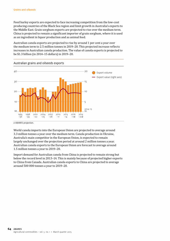
64
Grains and oilseeds
ABARESAgricultural commodities – vol. 5 no. 1 • March quarter 2015
Feed barley exports are expected to face increasing competition from the low-cost producing countries of the Black Sea region and limit growth in Australia’s exports to the Middle East. Grain sorghum exports are projected to rise over the medium term. China is projected to remain a significant importer of grain sorghum, where it is used as an ingredient in liquor production and as animal feed.
Australian canola exports are projected to rise by around 1 per cent a year over the medium term to 2.5 million tonnes in 2019–20. This projected increase reflects increases in Australian canola production. The value of canola exports is projected to be $1.3 billion (in 2014–15 dollars) in 2019–20.
Australian grains and oilseeds exports
Export volume
Mt2014–15$b
Export value (right axis)
10
40
20
30
5
10
15
20
z ABARES projection.
2019–20z
2016–17z
2013–14
2010–11
2007–08
2004–05
2001–02
1998–99
1995–96
World canola imports into the European Union are projected to average around 3.3 million tonnes a year over the medium term. Canola production in Ukraine, Australia’s main competitor in the European Union, is expected to remain largely unchanged over the projection period at around 2 million tonnes a year. Australian canola exports to the European Union are forecast to average around 1.5 million tonnes a year to 2019–20.
Import demand for Australian canola from China is projected to remain strong but below the record level in 2013–14. This is mainly because of projected higher exports to China from Canada. Australian canola exports to China are projected to average around 500 000 tonnes a year to 2019–20.

65
Grains and oilseeds
ABARESAgricultural commodities – vol. 5 no. 1 • March quarter 2015
Use and supply of barley in China
Use of barley in China
Barley use in China averaged 4.8 million tonnes a year over the 15 years to 2014–15. Food, seed and industrial (FSI) uses accounted for the largest share, at around 80 per cent. FSI use grew steadily from around 3 million tonnes a year in 2000–01 to around 4 million tonnes a year in 2013–14. FSI use is forecast to increase to 4.2 million tonnes in 2014–15.
The main FSI use of barley in China is in the manufacture of malt for use in the production of beer. China is the world’s largest producer of beer and production has grown at an average of 7 per cent a year over the past 15 years. In 2013 per person consumption of beer in China was 36.5 litres, compared with 17.4 litres in 2000. However, demand for malting barley has increased at a slower rate than the increase in beer consumption for two reasons. First, low alcohol beers have grown in popularity and require a smaller quantity of barley to produce a litre of beer than regular strength beers. Second, substitutes for barley, including wheat and grain sorghum, have been used increasingly to manufacture malt.
Barley use in China
Mt
Feed
Food, seed and industrial
f ABARES forecast.
1
2
3
4
5
7
6
2014–15f
2012–13
2010–11
2008–09
2006–07
2004–05
2002–03
2000–01
Barley is also used as feed by livestock producers in China, but this use varies considerably from year to year depending on the relative price of barley to other feed grains. In 2013–14 the use of barley for feed increased eightfold because the domestic price of corn had risen by more than 20 per cent in the previous three years.
continued ...

66
Grains and oilseeds
ABARESAgricultural commodities – vol. 5 no. 1 • March quarter 2015
Use and supply of barley in China continued
Barley supply in China
Domestic production
Barley production in China has fallen significantly over recent decades, reflecting a decline in the area harvested. Around 450 000 hectares of barley is expected to be harvested in China in 2014–15 and barley production is forecast to be around 1.6 million tonnes. This is largely unchanged from 2013–14 and the lowest in more than 50 years. Barley production in China peaked in 1966–67, when 6 million tonnes was produced from a harvested area of 3.8 million hectares.
Barley production in China
Production
Mt Mha
Harvested area(right axis)
0.5
1.0
1.5
2.0
2.5
3.0
3.5
0.2
0.4
0.6
0.8
1.0
1.2
1.4
2014–15f
2012–13
2010–11
2008–09
2006–07
2004–05
2002–03
2000–01
f ABARES forecast.
A major factor contributing to the long-term decline in barley production in China is the introduction of minimum support prices for the production alternatives of wheat, corn and rice. No minimum support price is set for barley in China.
Area harvested of broadacre grain crops in China
Mha
Oats
BarleyGrain sorghum
MilletWheat
Corn
f ABARES forecast.
10
20
30
40
50
70
60
2014–15f
2011–12
2008–09
2005–06
2002–03
1999–2000
1996–97
1993–94
1990–91
continued ...

67
Grains and oilseeds
ABARESAgricultural commodities – vol. 5 no. 1 • March quarter 2015
Use and supply of barley in China continued
Barley imports into China
The proportion of the barley supply in China coming from imports has increased over the past decade. In 2014–15 around 77 per cent of the barley supply in China is expected to be imported.
Barley supply in China
%
Imported
Domestically produced
f ABARES forecast.
20
40
60
80
100
2014–15f
2012–13
2010–11
2008–09
2006–07
2004–05
2002–03
2000–01
The volume of barley imported into China more than doubled in 2013–14 to 4.9 million tonnes, after averaging around 1.8 million tonnes a year over the previous 10 years. This followed a decision in December 2013 to ban imports of the genetically-modified corn variety MIR162. This most directly affected imports of feed corn from the United States and Argentina. In July 2014 the Chinese Government issued a further notice banning imports of distillers dried grain (DDGS) derived from MIR162 corn. DDGS is a by-product of corn-based ethanol production and is used as a relatively inexpensive alternative to feed grains.
Barley imports into China
Mt
Other
FranceCanada
Australia
Dec2014
Jun2014
Dec2013
Jun2013
Dec2012
Jun2012
Dec2011
Jun2011
Dec2010
Jun2010
0.25
0.50
0.75
1.00
1.25
1.50
1.75
2.00
continued ...

68
Grains and oilseeds
ABARESAgricultural commodities – vol. 5 no. 1 • March quarter 2015
Use and supply of barley in China continued
In 2014–15 and 2015–16, China’s barley imports are forecast to fall but remain high at 4.5 million tonnes and 4.1 million tonnes, respectively. This reflects lower demand for imported feed barley following a decision of the Chinese Government in December 2014 to lift the ban on imports of MIR162 corn and DDGS. Around one week after the ban was lifted, the state-owned China National Cereals, Oils and Foodstuffs Corporation ordered a 900 000 tonne shipment of DDGS for delivery between December 2014 and March 2015.
Australia is the largest supplier of barley to China, accounting for around 75 per cent of barley imports into China over the five years to December 2014. The other main suppliers are Canada and France. In 2013–14 the average import price of Australian barley in China was US$300 a tonne, compared with US$344 a tonne and US$326 a tonne for barley from Canada and France, respectively.
Australian barley exports to China
%
Non-malting grade
Malting grade
f ABARES forecast.
20
40
60
80
100
2014–15f
2012–13
2010–11
2008–09
2006–07
2004–05
2002–03
2000–01
Around 60 per cent of Australia’s barley exports to China is malting grade barley, which is used to manufacture malt for use in beer production. While total barley imports into China are forecast to fall in the short term, the demand for imported malting grade barley is forecast to remain strong.

69
Grains and oilseeds
ABARESAgricultural commodities – vol. 5 no. 1 • March quarter 2015
Outlook for wheat
unit 2012–13 2013–14 2014–15 f 2015–16 f 2016–17 z 2017–18 z 2018–19 z 2019–20 zunit 2012 13 2013 14 2014 15 f 2015 16 f 2016 17 z 2017 18 z 2018 19 z 2019 20 z
WorldArea illi h 215 220 222 225 225 225 226 227WorldArea million ha 215 220 222 225 225 225 226 227Yield t/ha 3.05 3.24 3.25 3.14 3.16 3.19 3.21 3.24/Production Mt 655 713 720 707 713 718 726 734Production Mt 655 713 720 707 713 718 726 734Consumption Mt 677 696 713 707 713 718 725 732Consumption Mt 677 696 713 707 713 718 725 732Closing stocks Mt 169 185 192 192 192 192 193 194Closing stocks Mt 169 185 192 192 192 192 193 194T dTrade Mt 141 155 151 147 148 150 152 154Stocks‐to‐use ratio % 25.0 26.6 26.9 27.2 27.0 26.7 26.6 26.5Stocks to use ratio % 25.0 26.6 26.9 27.2 27.0 26.7 26.6 26.5Price anominal US$/t 348 317 270 265 270 273 271 266
Price a– nominal US$/t 348 317 270 265 270 273 271 266real b US$/t 359 323 270 259 257 253 246 235– real b US$/t 359 323 270 259 257 253 246 235
AustraliaArea ’000 ha 12 979 13 473 13 808 13 890 13 890 13 910 13 941 13 959Area 000 ha 12 979 13 473 13 808 13 890 13 890 13 910 13 941 13 959Yield t/ha 1 76 2 00 1 71 1 76 1 79 1 82 1 84 1 85Yield t/ha 1.76 2.00 1.71 1.76 1.79 1.82 1.84 1.85Production kt 22 856 26 929 23 607 24 390 24 908 25 305 25 634 25 871Production kt 22 856 26 929 23 607 24 390 24 908 25 305 25 634 25 871E t lExport volume c kt 21 265 18 336 16 944 17 946 18 149 18 472 18 774 18 992Export value c– nominal A$m 6 776 6 103 5 426 6 066 6 243 6 422 6 491 6 445Export value c– nominal A$m 6 776 6 103 5 426 6 066 6 243 6 422 6 491 6 445– real d A$ 7 131 6 253 5 426 5 918 5 942 5 963 5 880 5 696– real d A$m 7 131 6 253 5 426 5 918 5 942 5 963 5 880 5 696
lAPW 10 net pool return – nominal A$/t 326 336 315 339 345 349 347 341
p nominal A$/t 326 336 315 339 345 349 347 341– real d A$/t 343 344 315 331 329 324 314 301– real d A$/t 343 344 315 331 329 324 314 301US 2 h d d i t h t f b d G lf J l J b I 2014 15 US d ll J l J d I 2014 15 A t li d lla US no. 2 hard red winter wheat, free on board Gulf, July–June. b In 2014–15 US dollars. c July–June years. d In 2014–15 Australian dollars.
f ABARES forecast. z ABARES projection.f ABARES forecast. z ABARES projection.Sources: ABARES; Australian Bureau of StatisticsSources: ABARES; Australian Bureau of Statistics
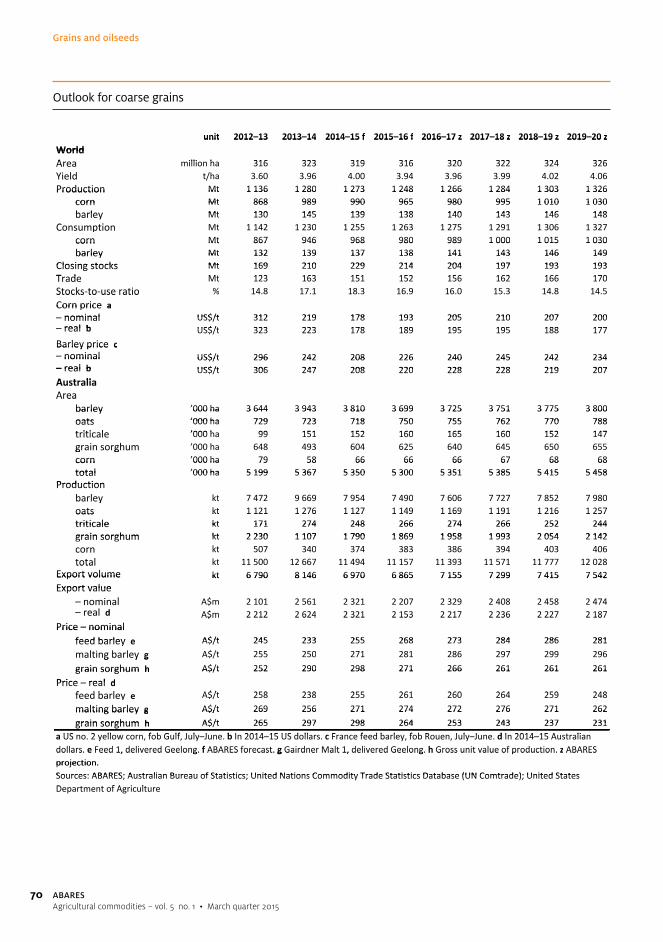
70
Grains and oilseeds
ABARESAgricultural commodities – vol. 5 no. 1 • March quarter 2015
Outlook for coarse grains
unit 2012–13 2013–14 2014–15 f 2015–16 f 2016–17 z 2017–18 z 2018–19 z 2019–20 zunit 2012 13 2013 14 2014 15 f 2015 16 f 2016 17 z 2017 18 z 2018 19 z 2019 20 z
WorldArea illi h 316 323 319 316 320 322 324 326WorldArea million ha 316 323 319 316 320 322 324 326Yield t/ha 3.60 3.96 4.00 3.94 3.96 3.99 4.02 4.06/Production Mt 1 136 1 280 1 273 1 248 1 266 1 284 1 303 1 326Production Mt 1 136 1 280 1 273 1 248 1 266 1 284 1 303 1 326
corn Mt 868 989 990 965 980 995 1 010 1 030corn Mt 868 989 990 965 980 995 1 010 1 030barley Mt 130 145 139 138 140 143 146 148barley Mt 130 145 139 138 140 143 146 148
C iConsumption Mt 1 142 1 230 1 255 1 263 1 275 1 291 1 306 1 327pcorn Mt 867 946 968 980 989 1 000 1 015 1 030corn Mt 867 946 968 980 989 1 000 1 015 1 030barley Mt 132 139 137 138 141 143 146 149barley Mt 132 139 137 138 141 143 146 149
Closing stocks Mt 169 210 229 214 204 197 193 193Closing stocks Mt 169 210 229 214 204 197 193 193T d Mt 123 163 151 152 156 162 166 170Trade Mt 123 163 151 152 156 162 166 170Stocks‐to‐use ratio % 14.8 17.1 18.3 16.9 16.0 15.3 14.8 14.5Stocks to use ratioCorn price aCorn price a– nominal US$/t 312 219 178 193 205 210 207 200– nominal US$/t 312 219 178 193 205 210 207 200real b US$/t 323 223 178 189 195 195 188 177– real b US$/t 323 223 178 189 195 195 188 177
Barley price cBarley price c– nominal US$/t 296 242 208 226 240 245 242 234 nominal US$/t 296 242 208 226 240 245 242 234– real b US$/t 306 247 208 220 228 228 219 207– real b US$/t 306 247 208 220 228 228 219 207A t liAustraliaArea
barley ’000 ha 3 644 3 943 3 810 3 699 3 725 3 751 3 775 3 800Area
barley 000 ha 3 644 3 943 3 810 3 699 3 725 3 751 3 775 3 800oats ’000 ha 729 723 718 750 755 762 770 788oats ’000 ha 729 723 718 750 755 762 770 788t iti l ’000 h 99 151 152 160 165 160 152 147triticale ’000 ha 99 151 152 160 165 160 152 147grain sorghum ’000 ha 648 493 604 625 640 645 650 655g gcorn ’000 ha 79 58 66 66 66 67 68 68corn 000 ha 79 58 66 66 66 67 68 68total ’000 ha 5 199 5 367 5 350 5 300 5 351 5 385 5 415 5 458total 000 ha 5 199 5 367 5 350 5 300 5 351 5 385 5 415 5 458
Productionb l k
Productionbarley kt 7 472 9 669 7 954 7 490 7 606 7 727 7 852 7 980yoats kt 1 121 1 276 1 127 1 149 1 169 1 191 1 216 1 257oats kt 1 121 1 276 1 127 1 149 1 169 1 191 1 216 1 257triticale kt 171 274 248 266 274 266 252 244triticale kt 171 274 248 266 274 266 252 244grain sorghum kt 2 230 1 107 1 790 1 869 1 958 1 993 2 054 2 142grain sorghum kt 2 230 1 107 1 790 1 869 1 958 1 993 2 054 2 142
kt 507 340 374 383 386 394 403 406corn kt 507 340 374 383 386 394 403 406total kt 11 500 12 667 11 494 11 157 11 393 11 571 11 777 12 028total kt 11 500 12 667 11 494 11 157 11 393 11 571 11 777 12 028
Export volume kt 6 790 8 146 6 970 6 865 7 155 7 299 7 415 7 542Export volume kt 6 790 8 146 6 970 6 865 7 155 7 299 7 415 7 542Export value
i l A$ 2 101 2 561 2 321 2 207 2 329 2 408 2 458 2 474Export value
– nominal A$m 2 101 2 561 2 321 2 207 2 329 2 408 2 458 2 474l– real d A$m 2 212 2 624 2 321 2 153 2 217 2 236 2 227 2 187A$m 2 212 2 624 2 321 2 153 2 217 2 236 2 227 2 187
Price – nominalfeed barley e A$/t 245 233 255 268 273 284 286 281
Price – nominalfeed barley e A$/t 245 233 255 268 273 284 286 281
l b l $/malting barley g A$/t 255 250 271 281 286 297 299 296g y ggrain sorghum h A$/t 252 290 298 271 266 261 261 261grain sorghum h A$/t 252 290 298 271 266 261 261 261
Price real df d b l A$/t 258 238 255 261 260 264 259 248
Price – real dfeed barley e A$/t 258 238 255 261 260 264 259 248ymalting barley g A$/t 269 256 271 274 272 276 271 262malting barley g A$/t 269 256 271 274 272 276 271 262grain sorghum h A$/t 265 297 298 264 253 243 237 231grain sorghum h A$/t 265 297 298 264 253 243 237 231
US 2 ll f b G lf J l J b I 2014 15 US d ll F f d b l f b R J l J d I 2014 15 A t lia US no. 2 yellow corn, fob Gulf, July–June. b In 2014–15 US dollars. c France feed barley, fob Rouen, July–June. d In 2014–15 Australian dollars. e Feed 1, delivered Geelong. f ABARES forecast. g Gairdner Malt 1, delivered Geelong. h Gross unit value of production. z ABARES dollars. e Feed 1, delivered Geelong. f ABARES forecast. g Gairdner Malt 1, delivered Geelong. h Gross unit value of production. z ABARES projection.projection.Sources: ABARES; Australian Bureau of Statistics; United Nations Commodity Trade Statistics Database (UN Comtrade); United StatesSources: ABARES; Australian Bureau of Statistics; United Nations Commodity Trade Statistics Database (UN Comtrade); United States D f A i lDepartment of Agriculture

71
Grains and oilseeds
ABARESAgricultural commodities – vol. 5 no. 1 • March quarter 2015
Outlook for oilseeds
unit 2012–13 2013–14 2014–15 f 2015–16 f 2016–17 z 2017–18 z 2018–19 z 2019–20 zunit 2012 13 2013 14 2014 15 f 2015 16 f 2016 17 z 2017 18 z 2018 19 z 2019 20 z
WorldWorldOilseedsOilseedsProduction Mt 475 505 530 522 517 531 547 562Consumption Mt 468 488 505 514 523 534 547 559Consumption Mt 468 488 505 514 523 534 547 559Closing stocks Mt 67 81 106 113 108 104 104 106Closing stocks Mt 67 81 106 113 108 104 104 106So beans indi ator pri e US$/t 597 547 423 390 440 452 452 437Soybeans indicator price a US$/t 597 547 423 390 440 452 452 437
l b $– real b US$/t 616 557 423 381 420 421 411 387$/Protein mealsProduction Mt 268 280 292 300 307 315 322 330Protein mealsProduction Mt 268 280 292 300 307 315 322 330Consumption Mt 264 275 287 297 308 316 324 332Consumption Mt 264 275 287 297 308 316 324 332l i kClosing stocks Mt 11 16 21 24 23 22 20 19g
Indicator price c US$/t 548 555 451 407 418 425 425 415Indicator price c US$/t 548 555 451 407 418 425 425 415– real b US$/t 567 565 451 397 398 395 386 367 real b US$/t 567 565 451 397 398 395 386 367Vegetables oilsP d ti M 161 170 175 180 186 192 198 204Vegetables oilsProduction Mt 161 170 175 180 186 192 198 204Consumption Mt 158 166 176 179 186 192 197 203Consumption Mt 158 166 176 179 186 192 197 203Closing stocks Mt 17 21 20 22 22 22 23 24Closing stocks Mt 17 21 20 22 22 22 23 24Indicator price d US$/t 1 162 985 841 804 804 812 800 777Indicator price d US$/t 1 162 985 841 804 804 812 800 777
l b US$/t 1 201 1 003 841 785 766 755 726 688– real b US$/t 1 201 1 003 841 785 766 755 726 688A liAustraliaTotal production kt 5 752 5 187 4 203 4 187 4 261 4 462 4 568 4 673Total production kt 5 752 5 187 4 203 4 187 4 261 4 462 4 568 4 673Winter kt 4 155 3 809 3 425 3 277 3 265 3 304 3 343 3 383Winter kt 4 155 3 809 3 425 3 277 3 265 3 304 3 343 3 383S mmer kt 1 597 1 378 779 910 996 1 158 1 225 1 290Summer kt 1 597 1 378 779 910 996 1 158 1 225 1 290C lCanolaArea ’000 ha 3 272 2 653 2 711 2 755 2 721 2 728 2 736 2 744Area 000 ha 3 272 2 653 2 711 2 755 2 721 2 728 2 736 2 744Production kt 4 142 3 795 3 413 3 264 3 252 3 290 3 329 3 369Production kt 4 142 3 795 3 413 3 264 3 252 3 290 3 329 3 369Export volume e kt 3 488 3 194 2 382 2 432 2 438 2 461 2 494 2 529Export volume e kt 3 488 3 194 2 382 2 432 2 438 2 461 2 494 2 529Export value e– nominal $m 2 094 1 929 1 251 1 373 1 401 1 437 1 443 1 445Export value e nominal $m 2 094 1 929 1 251 1 373 1 401 1 437 1 443 1 445– real g $m 2 204 1 976 1 251 1 339 1 334 1 334 1 307 1 277– real g $m 2 204 1 976 1 251 1 339 1 334 1 334 1 307 1 277P i h A$/t 560 529 485 528 543 550 544 541Price h A$/t 560 529 485 528 543 550 544 541
l– real g A$/t 590 542 485 516 516 510 493 478$/SunflowersArea ’000 ha 30 27 25 26 27 28 28 29SunflowersArea ’000 ha 30 27 25 26 27 28 28 29Prod ction kt 44 32 31 35 36 37 38 39Production kt 44 32 31 35 36 37 38 39Exports e kt 1 1 0 1 1 1 1 1Exports ePrice h A$/t 520 559 614 571 574 583 583 581Price h A$/t 520 559 614 571 574 583 583 581– real g A$/t 547 572 614 557 547 541 528 514– real g A$/t 547 572 614 557 547 541 528 514US 2 b f b G lf J l J b i b I 2014 15 US d ll S b l t i d f i ht R tt d 45 ta US no. 2 soybeans, fob Gulf, July–June basis. b In 2014–15 US dollars. c Soybean meal, cost insurance and freight, Rotterdam, 45 per cent
protein. d Soybean oil, Dutch, free on board ex–mill. e July–June. f ABARES forecast. g In 2014–15 Australian dollars. h Delivered Melbourne, protein. d Soybean oil, utch, free on board ex mill. e July June. f A AR S forecast. g In 0 4 5 Australian dollars. h elivered Melbourne,July–June. z ABARES projection.July–June. z ABARES projection.Sources: ABARES; Australian Bureau of Statistics; United States Department of AgricultureSources: ABARES; Australian Bureau of Statistics; United States Department of Agriculture

72 ABARESAgricultural commodities – vol. 5 no. 1 • March quarter 2015
SugarOutlook to 2019–20
Benjamin K Agbenyegah
• World sugar prices are forecast to be lower in the short term, reflecting expected record world sugar stocks resulting from increased world production in 2014–15.
• Over the medium term, higher world sugar consumption than production is projected to reduce world stocks. The world stocks-to-use ratio for sugar is expected to decline over the medium term.
• Reflecting expected higher Australian sugar production over the medium term, sugar exports are projected to reach 3.8 million tonnes in 2019–20.
Short-term outlookLower sugar prices to 2015–16The world indicator price for raw sugar (Intercontinental Exchange, nearby futures, no. 11 contract) is forecast to average US16 cents a pound in 2014–15 (October to September), around 5 per cent lower than in 2013–14. This forecast decline is driven by expected higher world sugar production in 2014–15, lifting world stocks to record levels. At this forecast level, the world indicator price will be around 20 per cent above the average of US13.3 cents a pound (in 2014–15 dollars) in the 10 years to 2009–10.
The world indicator price for raw sugar averaged around US17 cents a pound in 2013–14, compared with US18 cents a pound in 2012–13. As at 10 February 2015, the cumulative average price for sugar in the 2014–15 season was around US16 cents a pound, 9 per cent lower than the level reached in the same period in 2013–14.
In 2015–16 the world sugar indicator price is forecast to remain largely unchanged at an average of around US16 cents a pound, because the world stocks-to-use ratio is also expected to remain at 43 per cent. Growth in world sugar consumption is forecast to slightly outpace the rise in world production in 2015–16, leaving world sugar stocks largely unchanged at the end of the season, compared with the same time a year earlier.

73
Sugar
ABARESAgricultural commodities – vol. 5 no. 1 • March quarter 2015
Indicator price, Intercontinental Exchange (daily, ended 10 February 2015) a
USc/lbFeb2015
Apr2014
Jul2013
Sep2012
Dec2011
Feb2011
May2010
5
10
15
20
25
30
35
40
a Nearby futures, New York no. 11 contract.
World sugar indicators a
Production
Mt2014–15USc/lb
Real price (right axis)
Consumption
Closing stocks
50
100
150
200
250
7
14
21
28
35
2019–20z
2017–18z
2015–16f
2013–14
2011–12
2009–10
2007–08
2005–06
a Production, consumption and closing stocks are raw value equivalent and years are from October to September.f ABARES forecast. z ABARES projection.
World sugar production to remain highWorld sugar production is forecast to increase by 0.4 million tonnes in 2014–15 to around 183.0 million tonnes. This forecast reflects higher production in Europe, India, Mexico and Australia, partially offset by lower production in Brazil, China and Thailand. Favourable seasonal conditions led to improved sugar yields in Europe, India, Mexico and Australia. Forecast lower production in Brazil, China and Thailand is largely driven by estimated lower sugar yields, following above average yields in 2013–14.
In India, sugar production is forecast to be 28.5 million tonnes in 2014–15, up from 26 million tonnes in 2013–14. This forecast is largely driven by a 12 per cent increase in the average sugar yield, resulting from well above average monsoon rainfall in 2013. Partially offsetting this is a 2 per cent fall in the area of cane harvested in response to lower sugar prices.

74
Sugar
ABARESAgricultural commodities – vol. 5 no. 1 • March quarter 2015
Sugar production in Mexico is forecast to increase by 2 per cent in 2014–15 to 6.6 million tonnes. Sugar yields are estimated to increase by 2 per cent to 8 tonnes a hectare, following adverse seasonal conditions in 2013–14. The area harvested to cane is estimated to be similar to the previous year.
The 2014–15 sugar harvest in the European Union has been completed and is estimated to have been around 19.1 million tonnes, compared with 17.3 million tonnes in 2013–14. This forecast increase reflects an 11 per cent rise in sugar beet production as a result of record beet yields and a modest increase in the area planted to beet. Sugar yields are estimated to have increased by 7 per cent to 12 tonnes a hectare, following two years of adverse seasonal conditions.
Sugar production in Eastern Europe is estimated to have been 8.3 million tonnes in 2014–15, 11 per cent higher than in 2013–14. This forecast increase largely reflects the combined effect of a 22 per cent increase in the area planted to sugar beet and an estimated 28 per cent rise in average sugar yield in the Ukraine. Ukraine’s sugar production is estimated to have recovered by 56 per cent in 2014–15 to 2.1 million tonnes, following adverse seasonal conditions in 2013–14, which constrained beet planting and negatively affected yields. In the Russian Federation, sugar production is estimated to have remained largely unchanged at 4.8 million tonnes in 2014–15. The area planted to sugar beet increased by around 3 per cent to 930 000 hectares, but the average sugar yield is estimated to have declined by 7 per cent. Dry seasonal conditions in summer 2014 adversely affected beet and sugar yields.
US sugar production is estimated to have remained around 8 million tonnes in 2014–15. The area harvested to cane and sugar beet declined slightly to 803 000 hectares, but the average sugar yield is estimated to have increased slightly to 10 tonnes a hectare.
Sugar cane crush in Brazil is forecast to be 620 million tonnes in 2014–15, down from 653.3 million tonnes in 2013–14. This forecast is largely based on an estimated 5 per cent decline in average cane yield after drought adversely affected crops in Brazil’s centre south region, which produces around 90 per cent of Brazil’s sugar cane. Brazil’s sugar production is forecast to decline by 5 per cent in 2014–15 (October to September) to 37.5 million tonnes, reflecting the estimated fall in the cane crush and a rise in the share of cane allocated to ethanol.
In Brazil, sugar cane is used to produce both sugar and ethanol, with the relative prices of sugar and ethanol determining how much sugar cane is allocated to the production of each. World oil prices have fallen significantly in recent months but the Brazilian Government has put policy measures in place to encourage domestic ethanol consumption. These include a mandatory blending ratio with gasoline, guaranteed purchases by state-owned oil company Petrobras, low-interest rate loans for agro-industrial ethanol firms and lower excise tax on ethanol than on petrol. Anhydrous ethanol prices are also fixed at 59 per cent of the government-set gasoline price at the pump.
The mandatory blending ratio of anhydrous ethanol with gasoline in Brazil increased from 25 per cent to 27 per cent in February 2015. This follows an increase from 20 per cent to 25 per cent in 2013–14. The increase in mandatory blending is expected to lead to higher sugar cane intake for ethanol production. The share of cane allocated to ethanol production is expected to rise from around 55 per cent in 2013–14 to 57 per cent in 2014–15.

75
Sugar
ABARESAgricultural commodities – vol. 5 no. 1 • March quarter 2015
Sugar cane production and allocation, Brazil
Cane production
Mt %
Ethanol share (right axis)Sugar production
100
200
300
400
500
600
700
800
2019–20z
f ABARES forecast. z ABARES projection.
10
20
30
40
50
60
70
80
2017–18z
2015–16f
2013–14
2011–12
2009–10
2007–08
2005–06
2003–04
2001–02
Sugar production in China is forecast to be 13 million tonnes in 2014–15, 11 per cent lower than the record in 2013–14. This forecast is largely based on a 5 per cent decline in the area planted to cane in response to relatively low returns to growers compared with alternative crops, including fruits, cassava, vegetables and rice. The return to cane growers was lower because the Chinese Government reduced the price that millers pay for cane, from US$78 a tonne to US$72 a tonne in 2014–15. This reduction aims to assist mills that are struggling financially to stay in business, as well as to reduce domestic sugar production and stocks.
In Thailand, sugar production is forecast to be 11.5 million tonnes in 2014–15, down from 12.2 million tonnes in 2013–14. This forecast fall is mainly the result of an estimated 10 per cent decline in the average sugar yield, resulting from dry seasonal conditions. Partially offsetting this is a 4 per cent increase in the area planted to sugar cane to 1.5 million hectares. Growers increased the area planted to cane in response to favourable returns to cane production after the government redirected subsidies from rice to sugar cane production.
In 2015–16 world sugar production is forecast to increase to around 184 million tonnes. This largely reflects expected increases in production in Brazil, Thailand, Mexico and Australia, partially offset by lower forecast production in India, the European Union and China.
Sugar production in Brazil is forecast to recover from 37.5 million tonnes in 2014–15 to 39 million tonnes in 2015–16. An assumed return to favourable seasonal conditions, following dry weather in 2014–15, should improve cane and sugar yields in 2015–16. However, the Brazilian Government’s decision to increase the mandatory gasoline ethanol blending ratio from 25 per cent to 27 per cent in February 2015, combined with other policy measures to support the demand for ethanol, are expected to constrain sugar production growth. Around 58 per cent of the cane crush is expected to be allocated to ethanol production in 2015–16.
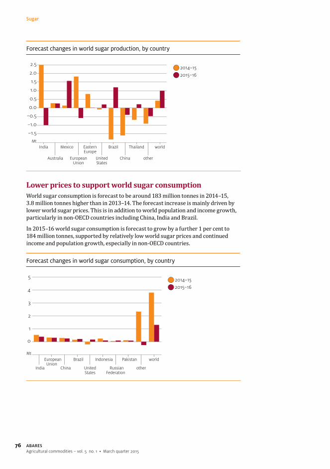
76
Sugar
ABARESAgricultural commodities – vol. 5 no. 1 • March quarter 2015
Forecast changes in world sugar production, by country
Mtworld
other
Thailand
China
Brazil
UnitedStates
EasternEurope
EuropeanUnion
Mexico
Australia
India
2014–152015–16
–1.5
–1.0
–0.5
0.0
0.5
1.0
1.5
2.0
2.5
Lower prices to support world sugar consumptionWorld sugar consumption is forecast to be around 183 million tonnes in 2014–15, 3.8 million tonnes higher than in 2013–14. The forecast increase is mainly driven by lower world sugar prices. This is in addition to world population and income growth, particularly in non-OECD countries including China, India and Brazil.
In 2015–16 world sugar consumption is forecast to grow by a further 1 per cent to 184 million tonnes, supported by relatively low world sugar prices and continued income and population growth, especially in non-OECD countries.
Forecast changes in world sugar consumption, by country
Mt
2014–152015–16
0
1
2
3
4
5
world
other
Pakistan
RussianFederation
Indonesia
UnitedStates
Brazil
China
EuropeanUnion
India

77
Sugar
ABARESAgricultural commodities – vol. 5 no. 1 • March quarter 2015
Record world sugar stocks in the short termWorld sugar stocks are forecast to increase slightly to a record 78.4 million tonnes in 2014–15. Despite world stocks reaching record levels, the stocks-to-use ratio for sugar is expected to be 43 per cent in 2014–15, down from around 44 per cent in 2013–14. This decline reflects expected higher world consumption growth relative to production. The forecast reduction in the stocks-to-use ratio will be the first since 2009–10.
In 2015–16 world sugar stocks are forecast to remain largely unchanged at around 78.4 million tonnes. The world stocks-to-use ratio is also expected to remain at 43 per cent.
World sugar consumption and stocks changes, and stocks-to-use ratio
StocksConsumption
Mt
–10
–5
0
5
10
15
%
Stocks-to-useratio (right axis)
10
20
30
40
50
60
2019–20z
f ABARES forecast. z ABARES projection.
2017–18z
2015–16f
2013–14
2011–12
2009–10
2007–08
2005–06
2003–04
2001–02
World sugar exports higher in 2015–16World sugar exports are forecast to recover by 0.6 million tonnes in 2014–15 to 58.5 million tonnes in 2014–15. Sugar supplies available for export are forecast to be higher in Thailand, India, the European Union and Australia. Partially offsetting this is an expected reduction in exports from Brazil—the world’s largest exporter. Lower sugar exports from Brazil reflect a forecast decline in production in 2014–15. Thai sugar production is also forecast to be lower in 2014–15, but large carry-over stocks from the record harvest of 2013–14 are expected to increase the amount of sugar available for export. India is expected to increase its sugar exports in 2014–15 because the Indian Government recently announced it would continue with the sugar export subsidies it introduced in 2013–14.
World sugar exports are forecast to increase by a further 4 per cent in 2015–16 to around 61 million tonnes, mainly as a result of an expected recovery in Brazil’s sugar exports.

78
Sugar
ABARESAgricultural commodities – vol. 5 no. 1 • March quarter 2015
Australian sugar returns to increase in 2015–16Queensland Sugar Limited, the marketer of more than 90 per cent of Australia’s raw sugar exports, estimated its harvest pool return to be $410 per tonne International Polarity Scale (IPS) in 2014–15, around 5 per cent higher than the seasonal pool return in 2013–14. The harvest pool arrangement replaced Queensland Sugar Limited’s seasonal pool arrangement in 2012–13.
In 2014–15 the average mill-gate return to Australian cane growers is forecast to decline by 1 per cent to $36 a tonne. Largely offsetting the effects of falling world prices is the assumed depreciation of the Australian dollar and higher sugar content in cane. The forecast return will be the lowest since 2007–08, when growers received around $32 a tonne (in 2014–15 dollars).
The return to Australian cane growers is forecast to be around $39 a tonne in 2015–16. This mainly reflects the combined effect of the assumed lower Australia dollar and expected higher sugar content in cane.
Modest growth in Australian sugar productionThe area harvested to cane is estimated to be 381 000 hectares in 2014–15, compared with 375 000 hectares in 2013–14. Australian sugar cane crushing in 2014–15 is complete, and average cane and sugar yields are estimated to have increased by 4 per cent to 84 tonnes a hectare and 6 per cent to 12 tonnes a hectare, respectively. The rise in average yields follows the adverse effects of flooding and the spread of canopy syndrome disease on cane in the Bundaberg and Isis regions of Queensland in 2013–14.
Australian area harvested of sugar cane and sugar yield
Area harvested
Mt t/ha
Sugar yield (right axis)
100
200
300
400
500
3
6
9
12
15
2019–20z
f ABARES forecast. z ABARES projection.
2017–18z
2015–16f
2013–14
2011–12
2009–10
2007–08
2005–06
2003–04
2001–02
Reflecting increases in the harvested area and average yields, Australian sugar production is estimated to be 4.7 million tonnes (raw value equivalent) in 2014–15, 7 per cent higher than in 2013–14. This level of production is the highest since 2007–08, when Australia produced 4.8 million tonnes. In 2015–16 Australian sugar production is forecast to increase by a further 6 per cent to 5 million tonnes, reflecting forecast higher cane plantings and sugar yields.

79
Sugar
ABARESAgricultural commodities – vol. 5 no. 1 • March quarter 2015
Australian sugar production, exports and returns to cane growers
ProductionExports
kt2014–15$/t
Return to cane growers(right axis)
1
2
3
4
5
6
10
20
30
40
50
60
2019–20z
f ABARES forecast. z ABARES projection.
2017–18z
2015–16f
2013–14
2011–12
2009–10
2007–08
2005–06
2003–04
2001–02
Australian sugar exports are forecast to be 3.4 million tonnes in 2014–15, 10 per cent larger than the 2013–14 shipments. This forecast reflects an increase in sugar supplies available for export. Australian sugar exports are forecast to increase by a further 7 per cent in 2015–16 to 3.6 million tonnes. Despite forecast lower world prices, the value of Australian sugar exports is forecast to rise by 10 per cent in 2014–15 to $1.5 billion, driven by higher sugar production and an assumed depreciation of the Australian dollar. Exports are forecast to reach $1.7 billion in 2015–16.
Medium-term outlook to 2019–20Sugar demand to support world pricesThe world indicator price for sugar is projected to increase over the medium term to average around US18 cents a pound (in 2014–15 dollars) in 2019–20. This projection of world indicator price largely reflects expected higher growth in world sugar consumption relative to production, which will reduce world stocks by a significant volume over the next few years.
World sugar production is projected to rise by an average 2.3 million tonnes a year from 2016–17 to reach 193.3 million tonnes in 2019–20. This projected increase is based on an assumption of average seasonal conditions in major sugar producing countries and improved production in some smaller producing countries in response to productivity increases. The projected increase in world sugar prices in the latter part of the outlook period is expected to provide incentives for higher sugar production.
World sugar consumption is projected to grow at an annual rate of 1.7 per cent from 2016–17 to reach a record 197 million tonnes in 2019–20. This projection largely reflects the effect on world sugar consumption of rising world population and continued income growth in non-OECD countries, particularly in India, China and Brazil. The rate of growth in world sugar consumption is projected to be faster in the earlier years of the projection period because of forecast lower prices and to gradually slow towards the end of the projection period.

80
Sugar
ABARESAgricultural commodities – vol. 5 no. 1 • March quarter 2015
Sugar production prospects for major producersSugar production in Brazil is projected to increase to 46 million tonnes in 2019–20, 20 per cent higher than forecast in 2014–15. Brazil has a large amount of suitable land to expand sugar cane production. In 2012 the Brazilian Government announced a loan package of US$2.2 billion to support sugar cane production. This package is for replacing ageing cane plantings and bringing new land into cane production. The demand for sugar cane for ethanol in Brazil is also expected to rise over the medium term because the Brazilian Government is expected to continue to raise the ratio of mandatory blending of anhydrous ethanol in gasoline. By 2019–20 the share of cane for ethanol production is expected to rise to 59 per cent, compared with an expected 57 per cent in 2014–15.
In India, sugar production is projected to reach 33 million tonnes in 2019–20, slightly above the record of 31 million tonnes in 2006–07. Depending on rainfall during the Indian monsoon, sugar production in India can fluctuate widely from season to season. India is expected to invest in the construction of more irrigation dams to reduce the reliance of sugar production on monsoon rainfall. The Indian Government is expected to continue the scheme of minimum support prices for raw and refined sugar to support sugar production.
In the European Union, the quota system ends in 2017 and higher sugar beet planting is expected to follow. EU sugar production is projected to increase to 21.2 million tonnes in 2019–20, 11 per cent higher than the forecast for 2014–15.
In the Russian Federation, sugar production is being encouraged by policies aimed at achieving more than 90 per cent self-sufficiency in meeting higher domestic demand. Sugar production is projected to be 5.8 million tonnes in 2019–20, 1 million tonnes more than forecast production in 2014–15.
For Europe as a whole, the sugar beet producing countries are projected to produce 29 million tonnes of sugar by 2019–20, compared with a forecast 26 million tonnes in 2014–15.
Sugar production in Thailand is projected to reach 14 million tonnes in 2019–20, compared with 11.5 million tonnes forecast in 2014–15. Higher world sugar prices in the latter part of the projection period, and the Thai Government’s policy of investing in new mills and support for ethanol production, are expected to provide incentives for shifting rice and cassava to sugar cane production. Sugar production in Thailand is also being encouraged through administered sugar prices for domestic consumption set at levels higher than world prices.
In the United States, sugar production is projected to reach 9 million tonnes in 2019–20, 13 per cent higher than forecast production in 2014–15. The US Government is expected to continue supporting its domestic cane and beet growers by keeping domestic sugar prices above world prices.
In Mexico, sugar production is projected to reach a record 8.5 million tonnes in 2019–20, in response to favourable returns to sugar production, which are being maintained above world levels because of access to the higher-priced US market under the North American Free Trade Agreement.

81
Sugar
ABARESAgricultural commodities – vol. 5 no. 1 • March quarter 2015
World sugar stocks-to-use ratio to fallWorld sugar stocks are projected to decline to around 64 million tonnes in 2019–20. This projection reflects higher growth in world consumption than production over the medium term. The world stocks-to-use ratio for sugar is expected to be 32.2 per cent in 2019–20, down from 43 per cent in 2014–15. At this projected level, the stocks-to-use ratio would be the lowest since 1990–91, when the ratio was 31.8 per cent.
Higher Australian sugar exports over the medium termThe area of sugar cane harvested in Australia is projected to expand to 409 000 hectares in 2019–20. This is higher than the average of 380 000 hectares for the 10 years to 2013–14, but well below the record 448 000 hectares in 2003–04. Suitable land close to existing sugar mills is limited and some cane land has been assigned to other uses, including forest plantation.
The sugar cane industry in the Ord River Irrigation Area (ORIA) in Western Australia peaked at a harvested area of 4100 hectares in 2003–04 and was shut down in 2007, when world sugar prices were low. However, interest in sugar production in the ORIA has been revived, particularly with the stage 2 expansion of the irrigated area. Chinese company, Shanghai Zhongfu, has successfully bid for a lease of 13 400 hectares of land. Any development in this region will have to abide by Indigenous land use rights and meet environmental management obligations. However, in order to profitably operate a sugar mill and begin commercialised sugar cane cultivation in the ORIA, Shanghai Zhongfu will have to acquire additional land in the Northern Territory. Shanghai Zhongfu is planting grain sorghum in the ORIA while negotiations are underway to acquire additional land in the Northern Territory.
Assuming favourable seasonal conditions over the medium term, Australian sugar production is projected to grow at an annual rate of 1 per cent from 2016–17 to around 5.3 million tonnes in 2019–20. Although this projection is above the estimated 4.7 million tonnes in 2014–15, it is below the record of 5.6 million tonnes produced in 1997–98.
Australian sugar exports are projected to be 3.8 million tonnes in 2019–20, up from 3.4 million tonnes expected in 2014–15. This compares with a record of 4.7 million tonnes shipped in 1997–98.

82
Sugar
ABARESAgricultural commodities – vol. 5 no. 1 • March quarter 2015
Outlook for sugar
unit 2012–13 2013–14 s 2014–15 f 2015–16 f 2016–17 z 2017–18 z 2018–19 z 2019–20 z
Production Mt 185.3 182.6 183.0 184.0 186.4 188.0 191.3 193.3– Brazil Mt 38.2 40.1 37.5 39.0 41.5 43.7 44.9 46.0Consumption Mt 175.7 178.9 182.7 184.0 189.7 192.5 194.9 197.0Exports Mt 61.1 57.9 58.5 60.7 61.6 62.7 63.8 65.0Closing stocks Mt 74.4 78.1 78.4 78.4 75.2 70.7 67.1 63.5Stocks‐to‐use ratio % 42.4 43.6 42.9 42.6 39.6 36.7 34.4 32.2
– nominal USc/lb 18.0 16.8 16.0 15.7 16.8 17.5 18.6 20.0– real c USc/lb 18.6 17.1 16.0 15.3 16.0 16.3 16.9 17.7
Production e kt 4 300 4 380 4 700 4 962 5 046 5 101 5 136 5 251Export volume kt 3 004 3 052 3 361 3 594 3 674 3 709 3 725 3 804
– nominal A$m 1 437 1 384 1 526 1 700 1 844 1 951 2 049 2 221– real g A$m 1 513 1 418 1 526 1 659 1 756 1 811 1 857 1 963a October–September years. b Nearby futures price, Intercontinental Exchange, New York, No. 11 contract. c In 2014–15 US dollars. d July–June years. e Raw tonnes actual. f ABARES forecast. g In 2014–15 Australian dollars. s ABARES estimate. z ABARES projection.Sources: ABARES; Australian Bureau of Statistics; Intercontinental Exchange; International Sugar Organization
World a
Australia d
Price b
Export value

83ABARESAgricultural commodities – vol. 5 no. 1 • March quarter 2015
• World cotton prices are forecast to fall over the short term, reflecting large world carry-over stocks and the termination of China’s policy to purchase cotton for stockpiling.
• Over the medium term, world cotton prices in real terms are projected to recover from 2016–17 onwards, reflecting projected lower world stocks as growth in consumption exceeds production.
• Australian cotton production is projected to increase over the medium term, almost doubling from a forecast low of 470 000 tonnes in 2014–15 to 818 000 tonnes in 2019–20.
Short-term outlookLower world cotton prices in 2015–16The world indicator price for cotton (Cotlook ‘A’ index) is forecast to fall by around 22 per cent in 2014–15 (August to July) to average US70 cents a pound, as a result of an expected rise in the world cotton stocks-to-use ratio to a record of around 96 per cent. The rise in the stocks-to-use ratio reflects large world carry-over stocks from 2013–14, the expectation of production exceeding consumption for the fourth consecutive year and a change in China’s cotton policy from stockpiling to income support for domestic producers.
From 2011–12 to 2013–14, China imported an average of 4.3 million tonnes of raw cotton, which had the effect of supporting world and Chinese domestic prices and encouraging production. In the 2014–15 season, China announced that it would end the strategic stockpiling of cotton and change its support for domestic cotton growers to direct payments. As a result, China is expected to limit its 2014–15 cotton imports to 894 000 tonnes, the minimum required under its World Trade Organization commitments. Following this change in China’s policy, the world indicator price for cotton fell from an average of US74 cents a pound in August 2014 to US67.4 cents a pound in January 2015.
In 2015–16 the world cotton indicator price is forecast to fall by a further 14 per cent to US60 cents a pound, as large world stocks continue to place downward pressure on prices. A major downside risk to this price forecast is the management of China’s large cotton stocks. If the Chinese Government decides to release cotton holdings onto the world market, prices could average significantly lower than currently forecast.
CottonOutlook to 2019–20
Benjamin K Agbenyegah

84
Cotton
ABARESAgricultural commodities – vol. 5 no. 1 • March quarter 2015
World cotton indicators
Production
Mt2014–15USc/lb
Indicator price (right axis)
ConsumptionClosing stocks
5
10
15
20
25
30
2019–20z
2017–18z
2015–16f
2013–14
2011–12
2009–10
30
60
90
120
150
180
f ABARES forecast. z ABARES projection.
Lower world cotton production in 2015–16World cotton production is forecast to be largely unchanged in 2014–15 at 26.2 million tonnes. The area planted to cotton is estimated to have increased by 5 per cent to 34.8 million hectares, reflecting an increase in government incentives for growers in India and Pakistan and an improvement in seasonal conditions in the United States. Offsetting the effect on production of this increase in area is an expected decline in average lint yield in India and Brazil as a result of dry seasonal conditions.
In 2015–16 world cotton production is forecast to decline by 5 per cent to 24.8 million tonnes. This forecast largely reflects an expected 7 per cent reduction in world cotton area, to 32 million hectares, in response to forecast lower world prices. In most major cotton producing countries, growers are expected to increase plantings of alternatives (such as grain sorghum, corn and soybeans), which are expected to provide more favourable returns than cotton. Partially offsetting the effect on production of this expected decline in area is an assumed 2 per cent rise in average lint yield, as seasonal conditions improve in some major producing countries that were affected by unfavourable seasonal conditions in 2014–15.
Forecast changes in world cotton production, by country
2014–15
2015–16
Mt
world
other
Turkey
Australia
Brazil
Pakistan
UnitedStates
India
China
–1.0
–0.5
0.0
0.5
1.0

85
Cotton
ABARESAgricultural commodities – vol. 5 no. 1 • March quarter 2015
Modest growth in world cotton consumption to 2015–16World cotton consumption is forecast to increase by 3 per cent in 2014–15 to 24.5 million tonnes. Growth in cotton apparel consumption in 2014–15 is expected to be strongest in China, India, Pakistan, Turkey and Bangladesh. In China, cotton consumption is forecast to increase for the first time in five years because domestic prices are expected to decline to the lowest levels in almost six years.
Although the polyester price has recently declined to its lowest level in five years, the price differentials between cotton and polyester have narrowed since mid 2014 because of a significant decline in cotton prices.
World weekly apparel fibre prices
USc/lb
Cotlook 'A' index
Polyester staple, China (cotton equivalent)
Polyester staple, Taiwan (cotton equivalent)
Jan2015
Sep2014
Apr2014
Nov2013
Jul2013
Feb2013
60
70
80
90
100
In 2015–16 world cotton consumption is forecast to increase by a further 3 per cent to 25.3 million tonnes, in response to the forecast further decline in world cotton prices. Given relatively low polyester prices, cotton consumption growth is likely to be constrained in the short term.
Share of world cotton consumption, by country
%
f ABARES forecast.
Other
TurkeyPakistan
IndiaChina
2015–16f
2013–14
2011–12
2009–10
2007–08
2005–06
2003–04
2001–02
20
40
60
80
100

86
Cotton
ABARESAgricultural commodities – vol. 5 no. 1 • March quarter 2015
World cotton stocks slightly lower in 2015–16World cotton stocks are forecast to rise by around 6 per cent in 2014–15 to a record 23.5 million tonnes. If realised, cotton stocks would be close to a year’s worth of world cotton consumption. China abolished its strategic stockpiling policy at the beginning of the 2014–15 season. As a result, the world excluding China is expected to account for the entire increase in world cotton stocks in 2014–15. World cotton stocks outside China are expected to rise for the first time in three years.
Cotton stocks
China
Mt
World excluding China
2
4
6
8
10
12
14
2015–16f
2013–14
2011–12
2009–10
2007–08
2005–06
2003–04
2001–02
f ABARES forecast.
Rising world cotton stocks are forecast to result in the world stocks-to-use ratio increasing by around 3 percentage points in 2014–15, to a record of around 96 per cent. For the world excluding China, the stocks-to-use ratio is forecast to rise to 60 per cent in 2014–15, up from 52 per cent in 2013–14. In contrast, the ratio for China is forecast to fall by around 13 percentage points to 169 per cent, largely reflecting strong consumption growth and lower cotton imports. The expected decline in China’s stocks-to-use ratio for cotton will be the first since 2010–11.
In 2015–16 world cotton stocks are forecast to ease by around 3 per cent to around 23 million tonnes, leading to a decline in the world cotton stocks-to-use ratio to 91 per cent. Despite a forecast rise in the stocks-to-use ratio for the world excluding China to 65 per cent in 2015–16, the ratio for China is expected to decline to 142 per cent.
World cotton exports are forecast to fall by around 16 per cent to 7.5 million tonnes in 2014–15, because of lower import demand by China. Supplies for export outside China are expected to decline because of lower production in major exporters, including Australia and Brazil, and higher domestic consumption in the United States and India. This trend is expected to continue in 2015–16, when world cotton exports are forecast to fall by a further 4 per cent to 7.2 million tonnes.

87
Cotton
ABARESAgricultural commodities – vol. 5 no. 1 • March quarter 2015
Australian cotton production to recover in 2015–16Australian cotton production is forecast to be 470 000 tonnes in 2014–15, compared with 885 000 tonnes in 2013–14. The area planted to cotton is estimated to have declined by 46 per cent to 210 000 hectares in response to relatively low cotton prices and dry seasonal conditions. Dry seasonal conditions in the lead-up to planting resulted in low soil moisture profiles, which restricted sowing to irrigated areas in 2014–15.
The average storage of public irrigation dams serving cotton growing regions of Australia declined from 44 per cent of total capacity on 12 February 2014 to 35 per cent on the same date in 2015. Current dam levels are 5 percentage points below the 10-year average to 2010.
Storage levels of main irrigation dams, at 12 February
Average of the 10 years to 2010
%
20142015
20
40
60
80
100
120
othe
r QLD
Bear
dmor
e (S
t Geo
rge)
Fairb
airn
(Em
eral
d)
Lesl
ie (D
arlin
g D
owns
)
othe
r NSW
Burr
endo
ng (M
acqu
arie
)
Pind
ari (
Mac
inty
re)
Keep
it (N
amoi
)
Gle
nlyo
n (M
acin
tyre
)
Cope
ton
(Gw
ydir)
Assuming a return to normal seasonal run-off between now and the start of the next planting window, in September 2015, the level of irrigation water in dams is expected to increase and support higher cotton production in 2015–16. Australian cotton production is forecast to rise by 19 per cent in 2015–16 to around 560 000 tonnes, reflecting a 19 per cent increase in planted area to 250 000 hectares and the assumption of average yield. Despite an assumed improvement in seasonal conditions in 2015–16, a larger increase in the area planted to cotton is expected to be constrained by relatively low returns for cotton compared with alternative crops (particularly grain sorghum).

88
Cotton
ABARESAgricultural commodities – vol. 5 no. 1 • March quarter 2015
Lower Australian returns in the short termBased on expected lower world cotton prices, the return to Australian cotton growers at the gin-gate in 2014–15 is forecast to average $490 a bale (227 kilograms) of lint (including the value of cottonseed and net of ginning costs), 6 per cent lower than the previous year. If realised, the forecast return to growers will be the lowest since 2005–06, when Australian cotton growers received $483 a bale (in 2014–15 dollars).
In 2015–16 the return to Australian cotton growers is forecast to fall by a further 8 per cent to $449 a bale, reflecting the forecast decline in world cotton prices being only partially offset by an assumed depreciation of the Australian dollar. The forecast return in 2015–16, compared with the forward cash price for the standard Australian cotton grade of $527 a bale offered on 11 February 2015.
Australian cotton exports lower in 2015–16Cotton exports from Australia are forecast to be 730 000 tonnes in 2014–15, compared with more than 1 million tonnes shipped in 2013–14. This forecast decline reflects lower cotton production in 2013–14 and 2014–15. Australia’s typical March-to-June harvest period means that cotton produced in one financial year is exported across two financial years. Despite this forecast fall, Australia is expected to maintain its position as the world’s third-largest cotton exporter in 2014–15—behind the United States and India.
In 2015–16 Australian cotton exports are forecast to decline by a further 34 per cent to around 483 000 tonnes, reflecting forecast lower cotton production in 2014–15. If realised, exports would be the lowest since 2010–11, when Australia shipped 505 000 tonnes of raw cotton.
Australian cotton production, exports and gin-gate returns
Production
kt2014–15$/bale
Gin gate return a (right axis)
Exports
200
400
600
800
1 000
1 200
1 400
100
200
300
400
500
600
700
2019–20z
2017–18z
2015–16f
2013–14
2011–12
2009–10
a Value of lint and cottonseed, less ginning costs. f ABARES forecast. z ABARES projection.
89
Cotton
ABARESAgricultural commodities – vol. 5 no. 1 • March quarter 2015
Medium-term outlookWorld cotton prices to recover in the medium termWorld cotton prices are projected to recover to average around US64 cents a pound (in 2014–15 dollars) in 2019–20, following a decline to US54 cents a pound (in 2014–15 dollars) in 2017–18. Over the medium term, strong consumption growth (particularly in non-OECD economies) is expected to exceed production growth to place upward pressure on world prices.
World cotton production is projected to increase at an annual rate of around 1.7 per cent from 2016–17 to reach 26.6 million tonnes in 2019–20. The increase in production mainly reflects a gradual rise in world cotton planting in response to expected growth in cotton consumption and an increase in world cotton prices. World cotton area is projected to grow at an annual rate of 1.6 per cent to reach 34 million hectares in 2019–20. Higher cotton production is projected in China, India, the United States, Pakistan, Australia and Brazil over the medium term.
Cotton production in China is projected to increase from its current low of 6.5 million tonnes in 2014–15 to reach 7.8 million tonnes in 2019–20. Despite this projected increase, cotton production is expected to remain below the record harvest of 8.1 million tonnes in 2007–08.
In 2019–20 India is projected to increase cotton production to 7.5 million tonnes, largely through yield and quality improvements. Although India is the world’s largest cotton producer by area planted, it has the lowest average lint yield of the major producing countries. India is expected to invest in construction of irrigation dams and to provide adequate electricity, to reduce the reliance of growers on the monsoon for crop performance.
In the United States, cotton production is projected to recover to 3.5 million tonnes in 2019–20, following a slight decline in 2015–16. This projection is based on an assumed return to normal seasonal conditions, following several years of adverse seasonal conditions in the major growing regions of Texas and the Mississippi Delta.
Pakistan’s cotton production is expected to reach around 2.5 million tonnes by the end of the projection period, largely reflecting yield improvements through the wider adoption of the current generation of genetically modified cotton varieties.
Brazil is projected to be a major contributor to the global production increase by the end of the projection period, with production projected to rise from a forecast 1.5 million tonnes in 2014–15 to 2.3 million tonnes in 2019–20. Brazil’s production gains are expected to be made through investments in irrigation and cotton research and development, which will expand the area planted to cotton and improve lint yields and quality.
Steady growth in world cotton consumptionWorld cotton consumption is projected to grow at an average rate of around 2.4 per cent a year from 2016–17 to reach 28 million tonnes by 2019–20. The main drivers of world cotton demand are expected to be strong income growth in non-OECD economies (including Pakistan, Turkey, Bangladesh and Brazil) and an assumed gradual recovery in major OECD economies.

90
Cotton
ABARESAgricultural commodities – vol. 5 no. 1 • March quarter 2015
World carry-over stocks of cotton are projected to ease over the medium term as consumption exceeds production. World stocks are projected to decline at an average of around 8 per cent a year from 2016–17 to reach around 17 million tonnes in 2019–20. This compares with the forecast record of 23.5 million tonnes in 2014–15. The world cotton stocks-to-use ratio is projected to decline to around 60 per cent in 2019–20. At this forecast level, the stocks-to-use ratio would still be around 5 percentage points higher than the 10-year average to 2012–13.
Stocks-to-use ratio for cotton
%
World excluding ChinaWorldChina
200
150
100
50
f ABARES forecast.
2015–16f
2013–14
2011–12
2009–10
2007–08
2005–06
Australian cotton prices to recover in 2019–20Driven by an expected recovery in world prices, returns to Australian cotton growers are projected to recover from $419 a bale in 2016–17 to average $453 a bale (in 2014–15 dollars) in 2019–20. This compares with the 10-year average to 2013–14 of $537 a bale (in 2014–15 dollars).
Under the assumption of average seasonal conditions, Australian cotton production is projected to increase at an annual rate of around 10 per cent a year from 2016–17 to reach 818 000 tonnes in 2019–20. Despite this projected rise, Australian cotton production is expected to remain well below the 1.2 million tonne record in 2011–12.
Production increases are projected to occur largely through an expansion in area, compared with 2014–15, as increased irrigation water availability and improved soil moisture profiles support higher sowings. Cotton lint yields in Australia are projected to remain largely unchanged over the medium term, because the uptake of the current generation of genetically modified cotton varieties is largely complete. In an average season more than 90 per cent of Australian cotton production is irrigated, and genetically modified varieties account for around 98 per cent of total planting.
Reflecting expected higher production, Australian cotton exports are projected to increase from a forecast 483 000 tonnes in 2015–16 to 778 000 tonnes in 2019–20.

91
Cotton
ABARESAgricultural commodities – vol. 5 no. 1 • March quarter 2015
Outlook for cotton
unit 2012–13 2013–14 s 2014–15 f 2015–16 f 2016–17 z 2017–18 z 2018–19 z 2019–20 zunit 2012 13 2013 14 s 2014 15 f 2015 16 f 2016 17 z 2017 18 z 2018 19 z 2019 20 z
World aProd ction Mt 26 9 26 2 26 2 24 8 24 9 25 0 25 9 26 6World aProduction Mt 26.9 26.2 26.2 24.8 24.9 25.0 25.9 26.6Consumption Mt 23.4 23.7 24.5 25.3 26.1 26.9 27.5 28.0Consumption Exports Mt 10.2 8.9 7.5 7.2 7.5 7.6 7.8 7.9Exports Mt 10.2 8.9 7.5 7.2 7.5 7.6 7.8 7.9Closing stocks Mt 19 6 22 1 23 5 22 9 21 7 19 8 18 2 16 7Closing stocks Mt 19.6 22.1 23.5 22.9 21.7 19.8 18.2 16.7St k t ti % 83 5 92 9 95 8 90 6 82 9 73 8 66 2 59 6Stocks‐to‐use ratio % 83.5 92.9 95.8 90.6 82.9 73.8 66.2 59.6Cotlook ’A’ index – nominal USc/lb 87.9 90.6 70.3 60.4 58.1 58.5 66.0 71.9– nominal USc/lb 87.9 90.6 70.3 60.4 58.1 58.5 66.0 71.9– real b USc/lb 90 8 92 3 70 3 59 0 55 4 54 4 59 8 63 7– real b USc/lb 90.8 92.3 70.3 59.0 55.4 54.4 59.8 63.7A t liAustralia cArea harvested ’000 ha 442.0 392.0 210.0 250.0 275.0 325.0 345.0 365.0Lint production kt 1 017.8 885.1 470.0 559.5 616.4 728.5 773.3 818.2Lint production kt 1 017.8 885.1 470.0 559.5 616.4 728.5 773.3 818.2Export volume kt 1 304 9 1 036 5 729 8 482 7 562 9 641 2 732 0 778 0Export volume kt 1 304.9 1 036.5 729.8 482.7 562.9 641.2 732.0 778.0E t lExport value– nominal A$m 2 694.8 2 355.4 1 546.3 998.3 1 148.8 1 319.7 1 603.8 1 789.2 nominal A$m 2 694.8 2 355.4 1 546.3 998.3 1 148.8 1 319.7 1 603.8 1 789.2– real d A$m 2 836.0 2 413.3 1 546.3 973.9 1 093.4 1 225.4 1 453.0 1 581.4 real d A$m 2 836.0 2 413.3 1 546.3 973.9 1 093.4 1 225.4 1 453.0 1 581.4a August–July years b In 2014–15 US dollars c July–June years d In 2014–15 Australian dollarsa August–July years. b In 2014–15 US dollars. c July–June years. d In 2014–15 Australian dollars.f ABARES f t ABARES ti t ABARES j tif ABARES forecast. s ABARES estimate. z ABARES projection.Sources: ABARES; Australian Bureau of Statistics; United States Department of AgricultureSources: ABARES; Australian Bureau of Statistics; United States Department of Agriculture

92 ABARESAgricultural commodities – vol. 5 no. 1 • March quarter 2015
HorticultureOutlook to 2019–20
Brian Moir and Jenny Eather
• The gross value of horticultural production is expected to increase gradually to $9.8 billion in 2019–20 (in 2014–15 dollars).
• For some fresh lines, the weaker Australian dollar and increased opportunities in Asia are expected to stimulate an increase in exports.
• The weaker dollar will improve the competitiveness of Australian processors, but pressure from imports will continue to be felt.
Markets in China and other Asian countries offer opportunities for Australian horticulture exporters. These export opportunities are expected to be enhanced by new trade agreements. The Korea–Australia Free Trade Agreement came into effect on 12 December 2014 and the Japan–Australia Economic Partnership Agreement on 15 January 2015. These agreements have resulted in the elimination of tariffs on many horticultural products exported to those countries, and further reductions are scheduled. Under the China–Australia Free Trade Agreement, tariffs will be removed on most horticultural products within the first four years of it coming into effect.
The Australian dollar has weakened in the past two years. This is expected to increase the competitiveness of Australian exports and to alleviate some of the pressure on Australian processors.
At around 50 per cent of capacity, water storage in the Murray–Darling Basin is at the lowest in four years but well above levels of 2002 to 2009. At these levels, water availability is not likely to constrain production in the short term.
The gross value of Australia’s horticulture industry is projected to increase to $9.8 billion (in 2014–15 dollars) by 2019–20, compared with a forecast $9.5 billion in 2014–15. The bulk of the increase in production is expected to be absorbed by the domestic market. The real value of exports of horticultural products is expected to increase between 2014–15 and 2019–20. Imports, predominantly of processed products, are expected to continue to increase strongly.

93
Horticulture
ABARESAgricultural commodities – vol. 5 no. 1 • March quarter 2015
Gross value of production
2014–15$b
Other horticulture
Fruit and nuts (excluding wine grapes)Vegetables
1
2
3
4
5
2019–20z
2016–17z
2013–14
2010–11
2007–08
2004–05
2001–02
z ABARES projection.Source: Australian Bureau of Statistics
Outlook for fruit and nutsThe gross value of Australian fruit and nut production, excluding wine grapes, is forecast to remain around $4.2 billion in 2015–16, following a forecast increase of 7 per cent in 2014–15. Export demand for some fruits, including table grapes and citrus, is expected to continue to stimulate production. Over the medium term to 2019–20, the gross value of Australian fruit and nut production is expected to increase to around $4.4 billion (in 2014–15 dollars).
Outlook for fruitFruit exports increased in the past four years following a decade of contraction. The recent expansion is primarily attributable to exports of fresh grapes, citrus, cherries and mangoes. Fruit exports grew by $240 million (in 2014–15 dollars) between 2010–11 and 2013–14; in this time exports of fresh grapes grew by $146 million, all citrus by $56 million, cherries by $26 million and mangoes by $10 million. Fruit exports are expected to continue to expand because of the assumed weaker Australian dollar and increased market opportunities, particularly in Asian countries. The value of Australian fruit exports in 2014–15 is forecast to strengthen a little to $732 million and to increase slowly to around $750 million (in 2014–15 dollars) by 2019–20.
Australia exports a diverse range of fruit to several countries. Fresh grapes and citrus, particularly navel oranges, were the main fresh fruit exports, with Hong Kong, New Zealand, Japan and Indonesia being the largest markets in 2013–14 in value terms.
Australian fruit exports to some Asian markets have grown rapidly in recent years. Between 2010–11 and 2013–14, the value of fruit exports to China, Vietnam and Hong Kong grew by 312 per cent, 227 per cent and 116 per cent, respectively, in real terms. This compares with growth of 48 per cent in fruit exports to all countries over the same period. Strong income growth and the popularity of fresh fruit as gifts have supported growth in these markets. Demand for high quality fruit produced by countries such as Australia is expected to grow strongly over the outlook period.

94
Horticulture
ABARESAgricultural commodities – vol. 5 no. 1 • March quarter 2015
However, market access is a factor constraining growth in exports of some fruit lines, particularly those that can be affected by fruit fly. In January 2015 Vietnam ceased issuing import permits for Australian produce, citing concerns about fruit fly contamination. Vietnam was Australia’s seventh largest export destination for fruit by value in 2013–14. The disruption to this market has serious consequences for table grape exporters. Australian fruit exports to Vietnam in 2013–14 were valued at $38 million, of which fresh grapes accounted for $30 million. The disruption caused oversupply and lower prices in the domestic market in early 2015.
The increasing value of fruit and nut imports, including processed products, first exceeded the value of exports in 2006–07 and has exceeded the value of exports by an increasing margin since. However, the value of fresh fruit exports continues to exceed the value of fresh fruit imports. Net export–import trade in fresh fruit and nuts reached a low in 2010–11 but increased in the following three years with the strengthening of Australia’s exports.
Fruit imports in 2013–14 were dominated by orange, apple and other fruit juices. Imports of processed fruit products are estimated to have increased (in 2014–15 dollars) from $445 million in 2001–02 to $757 million in 2013–14.
Kiwifruit, oranges, grapes and avocados were Australia’s major fresh fruit imports in 2013–14. The largest source of fresh fruit imports to Australia in value terms in 2013–14 was the United States, with imports of mainly citrus, grapes, peaches and cherries. These and other fresh fruit form part of the growing counter-seasonal trade, which has become important as consumers increasingly demand fresh fruit all year round. This demand can only be met by importing fruit during the non-producing months. Similar trends in other countries present opportunities for Australian exporters.
OrangesOrange production in 2014–15 is expected to increase a little to 434 000 tonnes. This is somewhat above levels of the previous few years and reflects adequate supplies of water, the maturing of earlier tree plantings and strong export markets. In 2015–16 orange production is forecast to increase further to 438 000 tonnes. The proportion of navel oranges in total orange production increased from less than 40 per cent in 2000–01 to 65 per cent 10 years later. Although data have not been available since 2010–11, the trend is expected to have continued. Navel oranges are predominantly sold to consumers on domestic and export markets. Valencias are mostly used for juicing and bring a smaller return to growers. Orange production is forecast to increase further in the medium term to around 455 000 tonnes in 2019–20.
Orange exports are forecast to remain unchanged in 2014–15 at around 125 000 tonnes. The weaker Australian dollar and improved access to Korea, Japan and China are expected to lead to increased exports during the medium term. Australia has been a counter-seasonal exporter and importer of oranges to and from the United States. While virtually all Australia’s orange imports continue to be sourced from the United States, other markets have increased in importance for Australian exports. During the 10 years to 2013–14, the volume of oranges sold to Japan increased almost fourfold to 31 500 tonnes, while sales to the United States halved to 10 400 tonnes. Exports to China also increased markedly to almost 10 000 tonnes in 2013–14, slightly less than exports to the United States.

95
Horticulture
ABARESAgricultural commodities – vol. 5 no. 1 • March quarter 2015
Australian orange, apple and banana production
’000tonnes
z ABARES projection.
Bananas
OrangesApples
2019–20z
2016–17z
2013–14
2010–11
2007–08
2004–05
2001–02
100
200
300
400
500
600
700
In recent years, Australian orange exports to the United States have faced strong competition from South Africa and Chile. The strengthening of the US dollar is expected to increase US demand for imported oranges. However, in 2014 the US dollar strengthened against the Chilean peso and the South African rand by more than it did against the Australian dollar, placing Australian exporters at a disadvantage.
ApplesApple production in Australia was fairly stable at around 300 000 tonnes a year in the four years to 2013–14. In 2013–14 apple production is estimated to have been 280 000 tonnes. In 2015–16 apple production is forecast to increase by about 2 per cent to about 290 000 tonnes, following a forecast increase of 2 per cent in 2014–15.
Apple exports have declined markedly over recent years. Almost 40 000 tonnes of fresh apples were exported in 2000–01, but exports averaged only 3 700 tonnes in the five years to 2012–13. In 2013–14 apple exports fell further to 2 100 tonnes. Over the medium term to 2019–20, some recovery is forecast as the lower value of the Australian dollar improves competitiveness. However, most Australian apple producers have difficulty competing in export markets. Unless efficiency in the industry improves, apple exports are likely to continue to have limited significance to the Australian industry.
China and New Zealand now meet Australia’s biosecurity requirements for the import of fresh apples. However, imports in 2010–11 amounted to only 700 tonnes and have been lower in recent years.
BananasBanana production reached 330 000 tonnes in 2012–13, reflecting recovery from the damage of Cyclone Yasi. The 2013–14 season was also one of good growing conditions, resulting in an estimated increase in banana production to 356 000 tonnes. It is forecast to fall by about 10 per cent to a more normal level of 321 000 tonnes in 2014–15.

96
Horticulture
ABARESAgricultural commodities – vol. 5 no. 1 • March quarter 2015
International markets exert no influence on the Australian banana industry. No country has met Australia’s biosecurity requirements for fresh banana imports and only a minimal quantity of fresh bananas (40 tonnes in 2013–14) is exported.
In late 2014 an eradication plan for the fungal disease banana freckle was announced, following detection of the disease in Cavendish bananas in the Northern Territory. The effect on national production will be limited because the Northern Territory accounts for only about 1 per cent of total production.
Outlook for tree nutsProduction of tree nuts has grown markedly in recent years, driven largely by almond production. In the three years from 2010–11 to 2013–14, almond production is estimated to have grown by almost 90 per cent, while macadamia production expanded by an estimated 18 per cent.
The gross value of tree nut production (almond, chestnut, hazelnut, macadamia, pecan, pistachio and walnut) is forecast to increase from an estimated $566 million in 2013–14 to $623 million in 2014–15.
Australian tree nut production
f ABARES forecast. z ABARES projection.
Other
WalnutsMacadamias
Almonds
20
40
60
80
100
120
140
160
’000tonnes
2019–20z
2017–18z
2015–16f
2013–14
2011–12
2009–10
2007–08
2005–06
Over the medium term, tree nut production is forecast to stabilise as tree plantings from the mid 2000s come to full maturity. The gross value of tree nut production is expected to expand from $623 million in 2014–15 to $668 million (in 2014–15 dollars) in 2019–20.
As production growth slows, exports are expected to continue to increase in the medium term but at a slower pace than in recent years. The value of tree nut exports is forecast to contract in 2014–15 to $539 million, from the record level of the previous year, and to then grow to around $649 million (in 2014–15 dollars) in 2019–20.

97
Horticulture
ABARESAgricultural commodities – vol. 5 no. 1 • March quarter 2015
AlmondsAlmond tree plantings reached between 5 000 and 7 000 trees a year in 2006 and 2007. Plantings subsequently tailed off, with virtually no plantings in 2012 and 2013. Consequently, the rapid expansion of almond production that occurred over the five years to 2014–15 (as trees came to maturity) has largely reached capacity. The production of almonds, which in 2014–15 is forecast at around 80 000 tonnes of kernel, is expected to reach 85 000 tonnes by 2019–20.
The Australian almond industry is largely export oriented. Australia is now the second-largest almond exporter in the world, although Australia’s exports remain far below the level of the United States. Almond exports amounted to around 48 000 tonnes of kernel in 2013–14. This is expected to increase to around 65 000 tonnes by 2019–20, with a value of $467 million (in 2014–15 dollars). World almond prices are expected to remain relatively firm over the medium term. Water scarcity in California is limiting new tree plantings, which will constrain growth in US production over the outlook period. At the same time, growth in global almond demand is expected to continue, lending support to Australia’s export returns.
Other tree nutsProduction of macadamias expanded strongly through two decades to the mid 2000s, when expansion ceased and production subsequently fluctuated from year to year. In 2013–14 favourable weather conditions led to a strong harvest, with production increasing by an estimated 10 per cent. Because the 2014 harvest extended longer into 2014–15 than usual, production in 2014–15 is also likely to be relatively high. The forecast for the medium term is for a modest increase in production. The gross value of production is expected to increase slightly to around $120 million (in 2014–15 dollars) by 2019–20.
In 2012–13 Australia was the world’s largest producer of macadamia nuts and exported about two-thirds of total production. However, South Africa was the largest exporter. Expansion of macadamia production in South Africa, the United States and Kenya is expected to maintain downward pressure on world prices, despite expected growth in global demand.
In the four years to 2012–13, the value of walnut exports increased 10 times in real terms to $20 million. Further growth is expected in the medium term, but walnut production and trade is much smaller than for almonds and macadamias.
Outlook for vegetablesThe gross value of Australian vegetable production increased from $3.2 billion (in 2014–15 dollars) in 2000–01 to almost $4 billion in 2012–13. Onions and tomatoes have been significant contributors to the increased production. The value of vegetable production is forecast to continue to expand, largely in line with domestic market requirements, to around $4.3 billion by 2019–20.
Vegetable exports contracted from $470 million in 2000–01 to $277 million in 2013–14 (in 2014–15 dollars). In the first half of 2014–15, the value of exports was 8 per cent higher than a year earlier, reflecting increased competitiveness because of the weaker Australian dollar. Exports are forecast to expand by 8 per cent in 2014–15 as a whole.

98
Horticulture
ABARESAgricultural commodities – vol. 5 no. 1 • March quarter 2015
Gross value of Australian vegetable production
2014–15$m
Other
TomatoesMushrooms
CarrotsOnionsPotatoes
1 000
2 000
3 000
4 000
5 000
z ABARES projection.
2019–20z
2016–17z
2013–14
2010–11
2007–08
2004–05
2001–02
The declining trend in exports is expected to slow in the medium term, as the weaker Australian dollar improves the competitiveness of Australian products and as the opportunities offered by trade agreements with China, Japan and the Republic of Korea are realised. However, Australian exporters of vegetables have limited capacity to compete with lower-cost exporters. The value of exports is expected to stabilise at around $300 million (in 2014–15 dollars) in the period to 2019–20.
Vegetable imports to Australia grew to $882 million in 2013–14. New Zealand, Italy, China and the United States are the largest suppliers of imported vegetables to Australia. Vegetable imports are dominated by processed vegetables, particularly potatoes, beans and tomatoes. Tomato ketchup and other sauces are also significant imports.
Imports of fresh vegetables in 2013–14 amounted to $71 million, 8 per cent of the total value of vegetable imports. Australia’s exports of fresh vegetables amounted to more than twice the value of fresh imports.
PotatoesPotato production changed little over the decade to 2013–14 and year-to-year fluctuations were much smaller than for many other crops. In 2012–13, 1.3 billion tonnes of potatoes were produced with a gross value of $690 million.
Producers of processing potatoes have come under increasing pressure from imports in the 10 years to 2013–14, with the value of potato imports growing fourfold to $143 million. New Zealand, the Netherlands, the United States and Belgium were the main suppliers of Australian potato imports in 2013–14.
The value of potato exports peaked at almost $60 million (in 2014–15 dollars) in 2010–11 but subsequently contracted to $40 million in 2013–14.
Potato production is expected to contract marginally through the medium term to around 1.2 billion tonnes in 2019–20, compared with 1.3 billion tonnes in 2012–13. This is because ongoing growth in the domestic market for fresh potatoes is expected to be more than offset by continuing pressure from imported processed potatoes and competition from other producing countries on export markets.

99
Horticulture
ABARESAgricultural commodities – vol. 5 no. 1 • March quarter 2015
TomatoesTomato production has recorded considerable year-to-year variation. In 2012–13 production increased by almost 25 per cent, to 455 700 tonnes.
Tomatoes are grown for fresh sales and for processing. Processors have come under strong competition from imports, with the real value of imports of tomatoes increasing by 62 per cent to $141 million in the 10 years to 2013–14. In 2013–14 the main source of imported tomatoes was Italy, with much smaller quantities being imported from China, the United States, Turkey and New Zealand.
The proportion of tomatoes grown for processing has dropped rapidly in recent years. In 2005–06, 61 per cent of Australian tomatoes were grown for processing. But by 2010–11, the latest year for which this information is available, only 32 per cent of tomatoes were grown for processing.
Tomato exports declined over the past decade, from $33 million in 2003–04 to $14 million in 2013–14 (in 2014–15 dollars).
The weaker value of the Australian dollar assumed over the medium term is expected to improve the competitiveness of Australian processors and exporters. However, any gains are likely to be modest; exports may be expected to grow slightly, while imports may stabilise rather than decline.
Australian tomato and potato production
Potatoes
’000tonnes
’000tonnes
Tomatoes (right axis)
f ABARES forecast. z ABARES projection.
300
600
900
1 200
1 500
150
300
450
600
750
2019–20z
2016–17z
2013–14f
2010–11
2007–08
2004–05
2001–02
1998–99
1995–96

100
Horticulture
ABARESAgricultural commodities – vol. 5 no. 1 • March quarter 2015
Outlook for horticulture
unit 2012–13 2013–14 s 2014–15 f 2015–16 f 2016–17 z 2017–18 z 2018–19 z 2019–20 zunit 2012 13 2013 14 s 2014 15 f 2015 16 f 2016 17 z 2017 18 z 2018 19 z 2019 20 z
Gross valuenominal A$ 9 020 9 231 9 489 9 821 10 130 10 448 10 776 11 114
Gross value– nominal A$m 9 020 9 231 9 489 9 821 10 130 10 448 10 776 11 114
l $– real a A$m 9 492 9 458 9 489 9 581 9 642 9 702 9 763 9 824$Fruit and tree nuts (excl. grapes) – nominal A$m 3 662 3 590 3 919 3 869 4 016 4 167 4 324 4 486Fruit and tree nuts (excl. grapes) – nominal A$m 3 662 3 590 3 919 3 869 4 016 4 167 4 324 4 486– real a A$m 3 854 3 679 3 919 3 775 3 822 3 870 3 917 3 965– real a A$m 3 854 3 679 3 919 3 775 3 822 3 870 3 917 3 965
blVegetables– nominal A$m 3 770 3 820 3 899 4 133 4 298 4 469 4 646 4 829
g nominal A$m 3 770 3 820 3 899 4 133 4 298 4 469 4 646 4 829– real a A$m 3 967 3 914 3 899 4 032 4 091 4 150 4 209 4 268 real a A$m 3 967 3 914 3 899 4 032 4 091 4 150 4 209 4 268Table and dried grapes
i lTable and dried grapes– nominal A$m 303 347 295 379 397 414 433 452$– real a A$m 319 355 295 370 378 385 392 400real a A$m 319 355 295 370 378 385 392 400Other horticultureOther horticulture– nominal A$m 1 285 1 474 1 376 1 439 1 419 1 397 1 373 1 347– nominal A$m 1 285 1 474 1 376 1 439 1 419 1 397 1 373 1 347real $– real a A$m 1 352 1 510 1 376 1 404 1 351 1 297 1 244 1 191
Exports– nominal A$m 1 478 1 865 1 824 1 962 2 023 2 081 2 137 2 194p nominal A$m 1 478 1 865 1 824 1 962 2 023 2 081 2 137 2 194– real a A$m 1 556 1 911 1 824 1 914 1 926 1 932 1 936 1 939– real a A$m 1 556 1 911 1 824 1 914 1 926 1 932 1 936 1 939F it
i lFruits– nominal A$m 634 724 732 754 777 800 824 849A$m 634 724 732 754 777 800 824 849– real a A$m 668 742 732 736 739 743 746 750 real a A$m 668 742 732 736 739 743 746 750Vegetablesnominal A$ 260 270 291 300 309 319 329 340
Vegetables – nominal A$m 260 270 291 300 309 319 329 340
l– real a A$m 273 277 291 293 295 296 298 300A$m 273 277 291 293 295 296 298 300Tree nuts– nominal A$m 348 610 539 644 671 694 714 734Tree nuts– nominal A$m 348 610 539 644 671 694 714 734– real a A$ 366 625 539 628 638 644 647 649– real a A$m 366 625 539 628 638 644 647 649Nursery– nominal A$m 12 11 11 9 8 6 7 6
y nominal A$m 12 11 11 9 8 6 7 6– real a A$m 12 12 11 9 8 6 6 5– real a A$m 12 12 11 9 8 6 6 5O h h i lOther horticulture– nominal A$m 224 250 252 255 258 262 263 266 nominal A$m 224 250 252 255 258 262 263 266– real a A$m 236 256 252 249 246 243 239 235– real a A$m 236 256 252 249 246 243 239 235I 2014 15 A t li d ll f ABARES f t ABARES ti t ABARES j ti a In 2014–15 Australian dollars. f ABARES forecast. s ABARES estimate. z ABARES projection.
Sources: ABARES; Australian Bureau of Statistics;

AgricultureLivestock

102 ABARESAgricultural commodities – vol. 5 no. 1 • March quarter 2015
Beef and vealOutlook to 2019–20
Beth Deards
• Strong international demand for Australian beef and veal has supported cattle prices in 2014–15.
• In early 2015 cattle prices were also supported by increased demand for restocker cattle as a result of widespread rainfall in many regions.
• In 2015–16 the weighted average saleyard price of beef cattle is forecast to increase by 16 per cent to 405 cents a kilogram (dressed weight).
• Strong export demand is expected to continue over the medium term, supported by an assumed lower Australian dollar and tariff reductions in some major markets.
• Live cattle exports are projected to remain high over the medium term.
Cattle prices to rise in 2015–16The weighted average saleyard price of beef cattle is forecast to increase by 19 per cent in 2014–15 to 349 cents a kilogram (dressed weight). Despite unfavourable seasonal conditions resulting in high cattle slaughter in the first half of the financial year, strong export demand for Australian beef and a depreciation of the Australian dollar supported cattle prices. Between July and November 2014, the weighted average saleyard price of beef cattle averaged 9 per cent higher year-on-year, even though Australian cattle slaughter was also 9 per cent higher year-on-year. Cattle prices rose further in December 2014 and January 2015. This followed widespread rainfall across major cattle producing regions that resulted in farmers increasing demand for restocker cattle (primarily young cattle). However, higher prices are expected to result in relatively high cattle slaughter continuing through the remainder of 2014–15.
Assuming average seasonal conditions, the weighted average saleyard price of beef cattle is forecast to increase by 16 per cent in 2015–16 to 405 cents a kilogram (dressed weight). Producers are expected to commence herd rebuilding in response to improved seasonal and market conditions by retaining heifers and increasing demand for restocker cattle. This will place further upward pressure on cattle prices, particularly for trade steers and medium cows. Additionally, strong export demand for Australian beef is expected to continue, supported by an assumed lower Australian dollar and tariff reductions in some major markets as a result of recently negotiated bilateral trade agreements.

103
Beef and veal
ABARESAgricultural commodities – vol. 5 no. 1 • March quarter 2015
Cattle prices are projected to increase again in 2016–17 as herd rebuilding activities continue and cattle slaughter falls further. Increasing international demand for Australian beef and veal is projected to keep cattle prices high in real terms in 2017–18 and 2018–19. In 2019–20, with an expanded cattle herd, cattle prices are projected to fall in real terms as slaughter increases.
Cattle and calf slaughter and weighted average saleyard price
Slaughter
millionhead
2014–15Ac/kg
Price (right axis)
f ABARES forecast. z ABARES projection.
2
4
6
8
10
100
200
300
400
500
2019–20z
2017–18z
2015–16f
2013–14
2011–12
2009–10
2007–08
2005–06
Slaughter and productionIn 2014–15 Australian cattle slaughter is forecast to be high at around 9.5 million head. During the first half of 2014–15, unfavourable seasonal conditions continued in many major cattle producing regions. This resulted in high cattle slaughter and destocking, particularly in eastern Australia. Between July and December 2014 slaughter of female cattle was 19 per cent higher year-on-year and male cattle slaughter was 4 per cent higher. Cattle slaughter is expected to remain relatively high through the remainder of 2014–15, with higher cattle prices expected to encourage producers to continue offloading cattle.
In 2014–15 Australian beef and veal production is forecast to be around 2.5 million tonnes, largely unchanged from the previous year. Average slaughter weights are expected to be similar to the reduced levels of 2013–14. This reflects a high proportion of female cattle slaughtered and unfavourable seasonal conditions during the first half of the year, which increased the incentive for producers to offload cattle at lighter weights.
Assuming average seasonal conditions in 2015–16, Australian cattle slaughter is forecast to fall by 6 per cent to 8.9 million head. As producers’ carrying capacity increases, significant herd rebuilding is expected to commence, reducing supply of cows for slaughter. Additionally, lower than average branding rates (the difference between the calving percentage and the percentage of calves lost between birth and branding) in the previous two years will reduce the supply of slaughter-ready cattle in 2015–16. In contrast, forecast higher cattle prices will provide strong incentives for producers to supply cattle for slaughter and favourable seasonal conditions are expected to lead to an increase in average slaughter weights. Overall, reduced cattle turn-off is forecast to lead to a 5 per cent fall in beef and veal production to 2.4 million tonnes.

104
Beef and veal
ABARESAgricultural commodities – vol. 5 no. 1 • March quarter 2015
Australian cattle slaughter is projected to fall a further 3 per cent in 2016–17 to 8.6 million head as herd rebuilding continues, assuming average seasonal conditions. Slaughter is projected to increase gradually over the rest of the medium term, to around 9.0 million head in 2019–20.
Cattle numbers to fall then recoverThe Australian cattle herd has declined significantly from its high of 29.3 million head at 30 June 2013. Herd liquidation was rapid during 2013–14 and the first half of 2014–15. Generally unfavourable seasonal conditions resulted in lower calving rates and higher than average mortalities. Slaughter and live export numbers were high, supported by strong international demand. In 2013–14 the proportion of the cattle herd (opening inventory as at 1 July 2013) slaughtered or exported live was around 36 per cent, the highest since 2002–03. In 2014–15 this proportion is forecast to rise to 37 per cent. The extent of herd liquidation is reflected in monthly female cattle slaughter numbers, which increased year-on-year every month from June 2012 to December 2014. By 30 June 2015 the cattle herd is forecast to fall to 27.0 million head.
Australian female cattle slaughter
’000head
2014–15
2013–142012–132011–12
100
200
300
400
500
JunMayAprMarFebJanDecNovOctSepAugJul
Australian cattle numbers are forecast to fall further in 2015–16. While calving rates are forecast to recover, additions to the cattle herd are expected to be largely offset by relatively high cattle slaughter and live exports. Assuming average seasonal conditions over the medium term, the cattle industry is projected to enter an expansionary phase from 2016–17, with cattle numbers gradually increasing to around 27.2 million head by 30 June 2020.

105
Beef and veal
ABARESAgricultural commodities – vol. 5 no. 1 • March quarter 2015
Strong demand for Australian beef to continueIn 2014–15 Australian beef and veal exports are forecast to increase by 3 per cent to more than 1.2 million tonnes. International demand for Australian beef and veal is forecast to be strong, supported by a fall in the Australian dollar and tariff reductions on imports into Japan and the Republic of Korea. The United States is forecast to be the largest market for Australian beef and veal in 2014–15, accounting for 34 per cent of total exports, compared with 22 per cent in 2013–14. Higher exports to Japan are also forecast.
Reflecting lower domestic supply, Australian beef and veal exports are forecast to fall by 5 per cent in 2015–16 to below 1.2 million tonnes, followed by a projected 3 per cent fall in 2016–17. However, international demand for Australian beef is expected to continue rising, leading to higher export unit values. From 2017–18 to 2019–20, Australian beef and veal exports are projected to increase in both volume and value terms. Over the projection period, Australian exports are expected to be more concentrated on the four major markets (Japan, United States, Republic of Korea and China) than in previous years.
Australian beef and veal exports
kt
f ABARES forecast. z ABARES projection.
Other
ChinaKorea, Republic of
JapanUnited States
2019–20z
2017–18z
2015–16f
2013–14
2011–12
2009–10
2007–08
2005–06
200
400
600
800
1 000
1 200
1 400
JapanAustralian beef and veal exports to Japan are forecast to rise by 7 per cent in 2014–15 to 300 000 tonnes. Australian beef has been subject to greater competition in Japan since the United States, post-BSE, re-entered the market in 2006 and, more particularly, when the age restriction was relaxed in 2013 to allow US beef imports from animals less than 21 months old. As a result, Australia’s market share fell from 90 per cent in 2004–05 to 53 per cent in 2013–14. In 2014–15 Australia’s market share is expected to increase as Australian beef gains a competitive advantage over US beef because of lower tariffs under the Japan–Australia Economic Partnership Agreement (JAEPA). The competitiveness of Australian beef in Japan will also benefit from an assumed greater appreciation in the US dollar, compared with the Australian dollar against the yen.

106
Beef and veal
ABARESAgricultural commodities – vol. 5 no. 1 • March quarter 2015
When JAEPA came into effect on 15 January 2015, the 38.5 per cent tariff on Australian beef imports was reduced to 30.5 per cent on frozen beef and 32.5 per cent on chilled beef. Further cuts of 2 per cent on frozen beef and 1 per cent on chilled beef are scheduled for April 2015. The tariff reductions under JAEPA are heavily frontloaded and are based on Japanese fiscal years (April to March), so Australian exporters will benefit from the largest tariff cuts before the middle of 2015. Over the next 15 years, these tariffs will reduce more slowly to 19.5 per cent on frozen beef and 23.5 per cent on chilled beef. Additionally, Japan’s 50 per cent global beef safeguard tariff—instigated to protect domestic producers in the event of a significant import surge—will no longer apply to beef imports from Australia. Japan’s global safeguard tariff (the so-called beef snapback) applies when total beef imports rise by more than 17 per cent relative to imports in the same period of the previous year. Instead, Australian imports will be subject to a specific safeguard, where a 38.5 per cent tariff will be applied to Australian beef when imports by Japan exceed a specified volume. In the first year of implementation, the trigger volume is 195 000 tonnes (shipped weight) for frozen beef and 130 000 tonnes for chilled beef. Trigger volumes will increase each year until the 10th year of implementation, when the trigger volumes will be 210 000 tonnes for frozen beef and 145 000 tonnes for chilled beef.
Australian beef and veal exports to Japan are forecast to rise by 7 per cent in 2015–16 to 320 000 tonnes, followed by a projected 5 per cent rise in 2016–17 to 335 000 tonnes. These increases largely reflect the effect of lower prices of Australian beef over US beef in the Japanese market. Additionally, US beef exports to Japan are projected to increase only gradually over this period because the US herd is expected to be in a rebuilding phase.
From 2017–18 to 2019–20, relatively sluggish economic growth is assumed for Japan and total beef imports are projected to increase only marginally. Australia is expected to remain an important supplier to Japan, and under JAEPA exports will continue to be supported by lower tariffs. However, increasing competition is expected from US exports because of an expected rise in US domestic beef supply following herd rebuilding. This is projected to lead to a small fall in Australian exports to Japan, particularly in higher value cuts, to around 330 000 tonnes in 2019–20.
Beef and veal imports, Japan
kt
Other
United States
Australia
f ABARES forecast.
100
200
300
400
500
600
2015–16f
2013–14
2011–12
2009–10
2007–08
2005–06

107
Beef and veal
ABARESAgricultural commodities – vol. 5 no. 1 • March quarter 2015
United StatesIn 2014–15 Australian beef and veal exports to the United States are forecast to rise by 58 per cent to 420 000 tonnes. Between July 2014 and January 2015, beef and veal exports to the United States were 114 per cent higher year-on-year. This was driven by lower US beef production, particularly cow beef production, resulting in record retail prices in the United States. The increase in export volume was supported by continued high production of manufacturing beef in Australia. Over the first six months of 2014–15, the average unit value of Australian beef and veal exports to the United States was $6.62 a kilogram. This compares with $6.08 a kilogram in Japan and $6.34 a kilogram in the Republic of Korea. The average unit value of Australian beef and veal exports to the United States was a record $7.47 a kilogram in December 2014.
Australian beef and veal exports to the United States
Volume
kt A$/kg
Unit value (right axis)
10
20
30
40
50
2
4
6
8
10
Dec2014
Aug2014
Apr2014
Dec2013
Aug2013
Apr2013
Dec2012
Aug2012
In 2015–16 Australian beef and veal exports to the United States are forecast to decline by 10 per cent to around 380 000 tonnes. Assuming average seasonal conditions, the United States is expected to continue herd rebuilding, retaining a higher proportion of female cattle. As a result cow slaughter will remain low, so demand for Australian manufacturing beef will continue to be high. However, lower supply of Australian manufacturing beef is expected to result in a fall in export volume. Additionally, the United States Department of Agriculture (USDA) forecasts beef retail prices to average higher in 2015 than the already elevated levels of 2014. With US supply of pork and poultry forecast to increase, some substitution away from beef consumption is expected.
Australian beef and veal exports to the United States are projected to fall a further 8 per cent in 2016–17 as Australian supply contracts further. Over the remainder of the projection period, Australian beef and veal exports to the United States are projected to rise. While US beef production is also expected to increase over this period, the USDA projects that rising exports and domestic consumption will lead to higher import demand.

108
Beef and veal
ABARESAgricultural commodities – vol. 5 no. 1 • March quarter 2015
Republic of KoreaAustralian beef and veal exports to the Republic of Korea are forecast to remain largely unchanged in 2014–15 at around 155 000 tonnes. In the first seven months of 2014–15 exports to the Republic of Korea were 8 per cent lower year-on-year. With Australian production forecast to remain relatively high in the second half of 2014–15, exports to Korea are forecast to rise, supported by tariff reductions under the Korea–Australia Free Trade Agreement (KAFTA).
KAFTA came into effect on 12 December 2014. Under KAFTA the 40 per cent tariff previously applied to imports of Australian beef will be phased out over 15 years, becoming duty-free in 2028. The United States, Australia’s major competitor in the market, also has a free trade agreement with Korea that was implemented in 2012, phasing out the 40 per cent tariff by 2026. US beef will continue to receive lower tariffs in the Korean market than Australian beef until 2028. In 2015 Australian beef imports into Korea will be subject to a 35 per cent tariff, while US beef will attract a 29 per cent tariff. The tariff differential will be a maximum of 5.3 per cent from 2015 through to 2026, compared with 8 per cent during most of 2014. In 2027 the tariff differential will be 2.7 per cent. In 2028 both countries will face zero tariffs.
In 2015–16 Australian beef and veal exports to the Republic of Korea are forecast to increase by 2 per cent to 158 000 tonnes. Beef production in Korea is expected to continue declining as producers take advantage of government assistance to exit the industry because of low profitability. This will result in higher demand for imports. Demand for Australian beef is also expected to be supported by a lower landed price than that of US beef, despite Australian beef facing a higher tariff than US beef. Korea is also an attractive market for Australian exporters because of generally higher returns compared with other major export markets. Over the medium term, Australian beef and veal exports to Korea are forecast to increase to 175 000 tonnes in 2019–20.
ChinaAustralian beef and veal exports to China are forecast to fall by 25 per cent in 2014–15 to 120 000 tonnes, followed by a further 2 per cent fall in 2015–16 to 118 000 tonnes. These falls largely reflect higher prices of Australian beef and greater competition from countries in South America. Between July and November 2014, Australian exports to China fell by 41 per cent year-on-year, while imports into China from Uruguay rose by 28 per cent. In November 2014 the average unit value of Australian beef imports into China was 44 per cent higher than beef imports from Uruguay.
Over the medium term, relatively strong economic growth in China will support beef consumption and it is expected to increasingly exceed domestic production, leading to higher imports. Australia is expected to be an important supplier of beef to China, with exports projected to increase from 2016–17. Competition from generally lower priced South American beef is expected to be strong in China, particularly if China begins importing beef from Brazil. In November 2014 the Chinese Government made an official bilateral agreement with the Brazilian Government to lift import restrictions on Brazilian beef. In January 2015 the market was also opened to Chile, with the Chinese Government awarding an export health certificate covering Chilean frozen beef and lamb. However, the China–Australia Free Trade Agreement (ChAFTA), once ratified, will support the competitiveness of Australian beef in the Chinese market.

109
Beef and veal
ABARESAgricultural commodities – vol. 5 no. 1 • March quarter 2015
Australian beef and veal exports to China
kt
f ABARES forecast. z ABARES projection.
30
60
90
120
150
180
2019–20z
2017–18z
2015–16f
2013–14
2011–12
2009–10
The most favoured nation (MFN) tariffs on beef imports into China are 25 per cent for frozen carcasses and half carcasses, 20 per cent for chilled carcasses and half carcasses, and 12 per cent for all cuts of chilled and frozen beef. Under ChAFTA, these tariffs will be eliminated over nine years for beef imported from Australia. Chilled and frozen carcasses accounted for less than 1 per cent of Australian beef exports to China in 2013–14. ChAFTA also includes a safeguard measure on Australian beef imports, where the MFN tariffs will be applied when imports into China exceed a specified volume. In the first year of implementation the trigger volume is 170 000 tonnes, 6 per cent greater than Australian exports to China in 2013–14. The threshold will gradually increase over the first 10 years of the agreement to a volume not available at the time of publication.
Live cattle exports to remain highIn 2014–15 Australian live feeder and slaughter cattle exports are forecast to remain high at around one million head. Between July and December 2014, Australian feeder and slaughter cattle exports were 38 per cent higher year-on-year to Indonesia and 95 per cent higher to Vietnam.
Since September 2013 the Indonesian Government has applied a reference price mechanism for live cattle imports. When the domestic retail price of secondary cuts exceeds the reference price, the government increases import permits and restricts them when the price falls below that level. The Indonesian Government recently announced its intention to increase the reference price from 76 000 rupiah to 85 000 rupiah. Prices have not fallen under the reference price since its inception. Over the first six months of 2014–15, average prices of secondary cuts in Indonesia were almost 50 per cent above the reference price and are likely to stay above it, at least in the short term.

110
Beef and veal
ABARESAgricultural commodities – vol. 5 no. 1 • March quarter 2015
Average prices of secondary beef cuts, Kebayoran Lama wet market, Jakarta
’000rupiah
Knuckle
ChuckShankReference price
20
40
60
80
100
120
140
24 Dec2014
31 Oct2014
28 Aug2014
26 Jun2014
25 Apr2014
28 Feb2014
27 Dec2013
25 Oct2013
30 Aug 2013
28 Jun2013
26 Apr2013
27 Feb2013
In January 2015 the Indonesian Government released March quarter 2015 import permits for 98 000 head of Australian cattle. This is around 30 000 head below the volume exported to Indonesia in the same quarter a year earlier. The government also reinforced the 350-kilogram weight limit for feeder and slaughter cattle imports. It is expected that any surplus heavier cattle no longer able to be exported to Indonesia will be absorbed by alternative markets without weight restrictions, such as Vietnam.
In 2015–16 feeder and slaughter cattle exports are forecast to fall by 10 per cent to 900 000 head. This reflects lower available supply of exportable cattle following two years of high Australian cattle slaughter and live exports. Export unit values are forecast to rise because demand for Australian live cattle is expected to be high in 2015–16.
Over the medium term, feeder and slaughter cattle exports are projected to recover to around one million head, with Indonesia expected to remain the primary market. Growth in Indonesian beef consumption is expected to exceed growth in domestic production over the medium term. As a result, imports will be required to assist in stabilising domestic prices. Demand is also expected to increase from Vietnam and Malaysia, as assumed relatively strong economic growth supports higher beef consumption. These are important markets for Australian live cattle exports because they do not impose weight or volume restrictions. Additional demand may come from new markets, including China, Thailand and Lebanon, if supply chains are developed in these countries and approved under the Exporter Supply Chain Assurance System.

111
Beef and veal
ABARESAgricultural commodities – vol. 5 no. 1 • March quarter 2015
Australian feeder and slaughter cattle exports
’000head
f ABARES forecast. z ABARES projection.
Other
MalaysiaIsrael
VietnamIndonesia
2019–20z
2017–18z
2015–16f
2013–14
2011–12
2009–10
2007–08
2005–06
200
400
600
800
1000
Outlook for beef and veal
unit 2012–13 2013–14 2014–15 f 2015–16 f 2016–17 z 2017–18 z 2018–19 z 2019–20 zunit 2012–13 2013–14 2014–15 f 2015–16 f 2016–17 z 2017–18 z 2018–19 z 2019–20 z
Saleyard price aSaleyard price a– nominal Ac/kg 297 293 349 405 425 437 449 450 nominal Ac/kg 297 293 349 405 425 437 449 450real b A /k 312 301 349 395 405 406 407 398– real b Ac/kg 312 301 349 395 405 406 407 398Ac/kg 312 301 349 395 405 406 407 398
Cattle numbers c million 29 3 28 5 27 0 26 5 26 6 27 0 27 3 27 2Cattle numbers c million 29.3 28.5 27.0 26.5 26.6 27.0 27.3 27.2– beef million 26 5 25 7 24 2 23 7 23 7 24 2 24 4 24 4– beef million 26.5 25.7 24.2 23.7 23.7 24.2 24.4 24.4Slaughterings ’000 8 457 9 473 9 475 8 900 8 600 8 650 8 750 9 000Slaughterings 000 8 457 9 473 9 475 8 900 8 600 8 650 8 750 9 000P d i k 2 245 2 464 2 473 2 359 2 279 2 292 2 328 2 394Production d kt 2 245 2 464 2 473 2 359 2 279 2 292 2 328 2 394Production d kt 2 245 2 464 2 473 2 359 2 279 2 292 2 328 2 394Consumption per person kg 32 6 31 0 28 0 26 9 25 6 25 5 25 1 25 3Consumption per person kg 32.6 31.0 28.0 26.9 25.6 25.5 25.1 25.3Consumption per person gExport volume e kt 1 014 1 184 1 223 1 158 1 119 1 126 1 151 1 187Export volume e kt 1 014 1 184 1 223 1 158 1 119 1 126 1 151 1 187p– to China kt 92 160 120 118 115 120 130 145– to China kt 92 160 120 118 115 120 130 145– to Japan kt 299 280 300 320 335 335 333 330– to Japan kt 299 280 300 320 335 335 333 330– to Korea, Rep. of kt 138 156 155 158 162 167 171 175– to Korea, Rep. of kt 138 156 155 158 162 167 171 175
U i d S k 207 266 420 380 350 350 355 355– to United States kt 207 266 420 380 350 350 355 355 to United States kt 207 266 420 380 350 350 355 355Export valueExport valuenominal A$m 4 871 6 265 8 014 8 144 8 093 8 377 8 634 8 905p
– nominal A$m 4 871 6 265 8 014 8 144 8 093 8 377 8 634 8 905l b– real b A$m 5 126 6 419 8 014 7 945 7 703 7 779 7 822 7 870 real b A$m 5 126 6 419 8 014 7 945 7 703 7 779 7 822 7 870
Li f d / l ht ttl t ’Live feeder/slaughter cattle exports ’000 513 996 1 000 900 900 950 975 1 000Live feeder/slaughter cattle exports 000 513 996 1 000 900 900 950 975 1 000i l A$ 339 780 850 810 833 893 921 940– nominal A$m 339 780 850 810 833 893 921 940 nominal $
– real b A$m 356 799 850 790 792 829 835 831– real b A$m 356 799 850 790 792 829 835 831a Dressed weight. b In 2014–15 Australian dollars. c At 30 June. d Carcass weight. e Fresh, chilled and frozen, shipped weight. f ABARES forecast. z ABARES projection.a Dressed weight. b In 2014–15 Australian dollars. c At 30 June. d Carcass weight. e Fresh, chilled and frozen, shipped weight. f ABARES forecast. z ABARES projection.
l f f l b k lSources: ABARES; Australian Bureau of Statistics; Department of Agriculture, Canberra; Meat & Livestock AustraliaSources: ABARES; Australian Bureau of Statistics; Department of Agriculture, Canberra; Meat & Livestock Australia

112 ABARESAgricultural commodities – vol. 5 no. 1 • March quarter 2015
Sheep meat and woolOutlook to 2019–20
Peter Berry
• The national sheep flock is forecast to decline to just under 71 million head by June 2015, before commencing a gradual rebuilding phase to reach around 76 million head by the end of 2019–20.
• Saleyard lamb prices are forecast to rise in 2015–16 as a result of lower turn-off, growing export demand and the effect of an assumed lower Australian dollar.
• The Australian Eastern Market Indicator price of wool is forecast to average around 1 075 cents a kilogram in 2015–16 and is projected to average 1 069 cents a kilogram in 2017–18 (in 2014–15 dollars) before declining slightly towards 2019–20.
Lamb price to rise in the short termAustralian lamb prices are forecast to increase by 7 per cent in 2014–15 to average 510 cents a kilogram. Strong export demand, particularly from the Middle East and the United States, is expected to drive this forecast rise.
Australian lamb saleyard price and slaughter
Lamb slaughter
millionhead
2014–15c/kg
Lamb saleyardprice (right axis)
150
300
450
600
750
5
10
15
20
25
f ABARES forecast. z ABARES projection.
2019–20z
2017–18z
2015–16f
2013–14
2011–12
2009–10
2007–08
2005–06
2003–04

113
Sheep meat and wool
ABARESAgricultural commodities – vol. 5 no. 1 • March quarter 2015
Strong export demand and dry seasonal conditions in some sheep producing regions resulted in high rates of turn-off during the 2014 spring. As a consequence, lower lamb availability through the summer placed upward pressure on prices. Prices are expected to remain relatively strong through the remainder of 2014–15 and in 2015–16, reflecting restocker demand as a result of an assumed return to average seasonal conditions. Growth in export demand—aided by an assumed lower Australian dollar—is also expected to place upward pressure on saleyard prices. Over the medium term (to 2019–20), prices are projected to decline gradually in real terms because flocks and slaughter are expected to increase.
Sheep prices to riseAssuming a return to average seasonal conditions in 2015–16, sheep prices are forecast to increase by 17 per cent to 364 cents a kilogram. This reflects a slowdown in adult sheep turn-off and greater restocker demand as producers begin to rebuild flocks. Flock rebuilding is expected to drive higher prices for breeding ewes in particular. As sheep numbers build up over the medium term and turn-off starts to rise again, saleyard prices are projected to decline gradually to average 323 cents a kilogram (in 2014–15 dollars) in 2019–20.
Australian sheep saleyard price and slaughter
Sheep slaughter
millionhead
2014–15c/kg
Sheep saleyardprice (right axis)
100
200
300
400
500
3
6
9
12
15
f ABARES forecast. z ABARES projection.
2019–20z
2017–18z
2015–16f
2013–14
2011–12
2009–10
2007–08
2005–06
2003–04
Wool prices to rise in 2015–16The Australian Eastern Market Indicator (EMI) wool price is forecast to be 2 per cent lower, at around 1 045 cents a kilogram in 2014–15. The average EMI price declined by 5 per cent year-on-year in the first six months of 2014–15, falling to a low of 1 001 cents a kilogram in August 2014. However, a depreciation of the Australian dollar and stronger export demand resulted in the EMI price increasing to 1 057 cents a kilogram in the last trading week in December, while wool offerings at auctions over the period July to December increased by 22 per cent year-on-year.
In 2015–16 the EMI is forecast to increase by 3 per cent to average 1 075 cents a kilogram. This is largely as a result of an assumed lower Australian dollar and a forecast increase in demand for woollen clothing and textiles in major consuming countries as income growth strengthens.

114
Sheep meat and wool
ABARESAgricultural commodities – vol. 5 no. 1 • March quarter 2015
Australian Eastern Market Indicator wool price, weekly
EMI (US$)
c/kgclean
Bales offered(right axis)
EMI
200
400
600
800
1 000
1 200
1 400
1 600
’000bales
10
20
30
40
50
60
70
80
23 Jan2015
11 Jul2014
31 Jan2014
12 Jul2013
25 Jan2013
13 Jul2012
27 Jan2012
15 Jul2011
Over the medium term, the EMI is projected to average around 1 069 cents a kilogram in 2017–18 (in 2014–15 dollars), supported by a modest increase in consumer demand, before declining marginally to around 1 064 cents a kilogram in real terms in 2019–20 as Australian wool production picks up in response to expected flock rebuilding.
Sheep flock rebuilding assumed in 2015–16Adverse seasonal conditions in 2013–14 and the first half of 2014–15, together with strong export demand for lamb and mutton, drove a significant rise in sheep turn-off. As a result, closing sheep numbers are expected to fall by 3 per cent to 70.7 million head by the end of 2014–15. However, assuming average seasonal conditions, sheep numbers are forecast to begin rebuilding, rising by 2 per cent to around 72 million head by the end of 2015–16.
Australian sheep flock
Lambs
millionhead %
Share of ewes in adult flock (right axis)
25
50
75
100
125
20
40
60
80
100
Non-breeding adultsheep (wethers)Ewes
f ABARES forecast. z ABARES projection.
2019–20z
2017–18z
2015–16f
2013–14
2011–12
2009–10
2007–08
2005–06
2003–04

115
Sheep meat and wool
ABARESAgricultural commodities – vol. 5 no. 1 • March quarter 2015
Over the medium term, the national sheep flock is projected to continue to rebuild, growing to around 76 million head by 2019–20. A slight increase in the proportion of breeding ewes in the flock is expected to contribute to higher lamb production as a result of an ongoing trend towards production of sheep meat. The proportion of non-breeding adult sheep in the flock—particularly wethers—is projected to decline, reflecting the shift away from wool production.
The pace of flock rebuilding will be tempered by expected strong export demand for sheep meat and hence relatively favourable prices for both lamb and sheep. Graziers will be facing the challenge of choosing between flock rebuilding and turn-off for favourable prices. Seasonal conditions will also be an important factor affecting flock rebuilding activity.
Lamb slaughter and production to fall in 2015–16Over the past two decades, the sheep industry has been shifting focus from wool to prime lamb production. As a result, lamb slaughter as a proportion of the total sheep flock has risen. In 2014–15 lamb slaughter is forecast to increase by 2 per cent to reach 22.3 million head, the highest since 1971–72, when the Australian sheep flock was more than twice its current size at 180 million head.
Average carcass weights in the first half of 2014–15 were around 3 per cent higher year-on-year as a result of better seasonal conditions in major producing regions in southern Australia. Reflecting both the increase in lamb slaughter and a forecast rise in carcass weights, lamb production is forecast to increase by 3 per cent to 488 000 tonnes in 2014–15.
In 2015–16 Australian lamb slaughter is forecast to fall by 4 per cent to around 21.5 million head, assuming farmers rebuild flocks in response to average seasonal conditions. The forecast decrease in lamb slaughter is expected to result in a 5 per cent decrease in lamb production to 466 000 tonnes in 2015–16. Over the medium term, lamb slaughter is projected to fall by around 1 per cent a year until 2017–18, before rising to 22.8 million head in 2019–20. Lamb production is projected to increase to around 517 000 tonnes in 2019–20.
Mutton production to fall sharply in 2015–16Adult sheep slaughter in Australia is estimated to fall by 9 per cent in 2014–15 to around 9.2 million head. Assuming a return to average seasonal conditions in 2015–16, sheep slaughter is forecast to decrease by 33 per cent to 6.2 million head. This is because more female sheep are expected to be retained for flock rebuilding and the availability of sheep for slaughter will decline. As a result, mutton production is forecast to fall by 35 per cent, from 221 000 tonnes in 2014–15 to 143 000 tonnes in 2015–16.
Over the medium term, adult sheep slaughter is projected to remain relatively low, assuming the national flock will continue to rebuild. In response to gradually increasing sheep numbers, slaughter of adult sheep is projected to rise slowly to around 6.5 million head in 2019–20. Mutton production is projected to increase to around 153 000 tonnes by 2019–20.

116
Sheep meat and wool
ABARESAgricultural commodities – vol. 5 no. 1 • March quarter 2015
Shorn wool production to declineShorn wool production is forecast to decline by around 4 per cent to 336 000 tonnes greasy in 2014–15, reflecting a decline in the number of sheep shorn and lower average fleece weights as a result of poor pasture conditions across parts of the eastern states.
In 2015–16 shorn wool production is forecast to fall by a further 2 per cent to 328 000 tonnes greasy. The volume of wool cut per head is also forecast to decline in 2015–16, reflecting an expected decline in the proportion of wethers in the sheep flock.
Shorn wool production is projected to increase slowly and reach 345 000 tonnes in 2019–20, largely reflecting the expected increase in the number of sheep shorn as the national flock rebuilds over the outlook period. A declining trend in the share of wethers in the Australian sheep flock is expected to result in the average cut per head falling to 4.3 kilograms by 2019–20. This compares with a forecast average cut of 4.4 kilograms in 2014–15.
Australian shorn wool production and price
Shorn woolproduction
kt 2014–15Ac/kg clean
EMI (right axis)
f ABARES forecast. z ABARES projection.
100
200
300
400
500
600
700
800
200
400
600
800
1 000
1 200
1 400
1 600
2019–20z
2017–18z
2015–16f
2013–14
2011–12
2009–10
2007–08
2005–06
2003–04
2001–02
1999–00
1997–98
1995–96
Improved seasonal conditions in many wool growing regions in southern Australia resulted in a lower proportion of finer micron wool produced. Data released by the Australian Wool Testing Authority indicate that around 44.5 per cent of wool tested in the first six months of 2014–15 was 19.5 microns or less, compared with 45.6 per cent over the same period in 2013–14.

117
Sheep meat and wool
ABARESAgricultural commodities – vol. 5 no. 1 • March quarter 2015
Domestic lamb consumptionAustralian lamb consumption per person has been in long-term decline, from 23.8 kilograms a person in 1971–72 to 8.9 kilograms a person in 2013–14. This decline largely reflects food consumption trends over the past several decades, with lower red meat consumption in favour of more poultry and seafood. Higher retail prices for lamb relative to other red meats have also affected consumer choice.
Domestic lamb consumption per person is forecast to remain at the current level over the next few years. Total domestic lamb consumption is expected to increase only marginally towards the medium term as Australia’s population increases.
Australian lamb production, exports and domestic consumption
Exports
kt cwe kg/person
Consumptionper capita (right axis)
Domestic consumption
s ABARES estimate.
3
6
9
12
15
100
200
300
400
500
2014–15s
2012–13
2010–11
2008–09
2006–07
2004–05
2002–03
2000–01
1998–99
1996–97
Lamb exports and market developmentsAustralian lamb exports are forecast to increase by 6 per cent to a record 240 000 tonnes (shipped weight) in 2014–15, reflecting continued strong international demand and the forecast rise in lamb slaughter. Lamb export earnings are forecast to increase by 12 per cent in 2014–15 to $1.64 billion.
In 2015–16 lamb export volumes are forecast to fall by 10 per cent to around 215 000 tonnes as a result of reduced availability in response to an expected decline in lamb slaughter. Lamb export earnings in 2015–16 are forecast to be 8 per cent lower at $1.5 billion.
Over the medium term, lamb exports are projected to fall to around 204 000 tonnes by 2017–18, as a result of flock rebuilding, before increasing to around 250 000 tonnes in 2019–20.

118
Sheep meat and wool
ABARESAgricultural commodities – vol. 5 no. 1 • March quarter 2015
Middle EastThe Middle East has been a major growth market for Australian sheep meat exports over the decade to 2013–14. Exports rose by more than 550 per cent over the period as demand strengthened in response to an expanding middle class and growing expatriate population.
Demand growth continued in the first half of 2014–15, with Australian lamb exports to the region increasing by 13 per cent year-on-year to around 34 700 tonnes. Exports to Jordan increased by 36 per cent to 9 100 tonnes in the period, making that country Australia’s largest export destination in the region. Exports to the United Arab Emirates, the second largest export destination, increased by 12 per cent to 8 900 tonnes. Exports to Qatar grew by 42 per cent to 5 900 tonnes. Bahrain emerged as a significant export destination for Australian lamb after Australian live sheep exports to the country were voluntarily suspended in August 2012. However, in the first half of 2014–15, Australian lamb exports to Bahrain declined by 19 per cent to 5 400 tonnes. Australian live sheep exports to Bahrain were around 149 600 head in the same period, compared with exports of 157 700 head in the six months before the voluntary suspension in August 2012.
In 2014–15 as a whole, lamb exports to the Middle East are forecast to increase by 8 per cent to 65 000 tonnes. In 2015–16 exports to the region are forecast to grow at a slower rate of 3 per cent to 67 000 tonnes, reflecting the expected decline in Australian lamb production. This tightening of export supplies is expected to limit growth in exports to the region in the next few years.
ChinaChina has become a major destination for Australian sheep meat exports over the past decade, reflecting strong growth in consumer demand. Growth in Chinese demand has been a result of an expanding urban population, with strong income growth and greater consumption of meat protein, including sheep meat. Lamb exports to China increased to 41 000 tonnes in 2013–14, compared with less than 12 000 tonnes four years earlier.
Continued growth in demand is expected to drive a 7 per cent increase in Australian lamb exports to China to 44 000 tonnes in 2014–15. In 2015–16 lamb exports are forecast to increase by a further 7 per cent to 47 000 tonnes. Over the medium term, exports to China are expected to grow more slowly, reaching around 59 000 tonnes by 2019–20.
United StatesThe United States is Australia’s largest market for lamb by value, with export earnings reaching $399 million in 2013–14. Although lamb remains a niche product in the United States, a recovering economy together with a depreciation of the Australian dollar have contributed to increased demand for Australian lamb in the United States.
In the first half of 2014–15, exports of lamb to the United States grew by 20 per cent year-on-year to 24 000 tonnes. In 2014–15 as a whole, Australian exports of lamb to the United States are forecast to increase by 11 per cent to 47 000 tonnes. In 2015–16 exports are forecast to increase by 4 per cent to 49 000 tonnes. Over the remainder of the projection period, Australian exports of lamb to the United States are projected to average around 50 000 tonnes a year.

119
Sheep meat and wool
ABARESAgricultural commodities – vol. 5 no. 1 • March quarter 2015
Australian lamb exports, by major destination
Other
kt swe
f ABARES forecast. z ABARES projection.
50
100
150
200
250
United StatesMiddle EastChina
2019–20z
2017–18z
2015–16f
2013–14
2011–12
2009–10
2007–08
2005–06
Competition with New ZealandAustralia and New Zealand are the world’s two largest exporters of sheep meat. New Zealand holds significant market access advantages over Australia in the major export markets of China and the European Union, as well as a more favourable exchange rate.
In 2013–14 New Zealand exported 94 500 tonnes of lamb into China, compared with Australian exports of 41 200 tonnes. The New Zealand–China Free Trade Agreement provides New Zealand with a competitive advantage as tariffs applied to China’s imports of New Zealand sheep meat have been reduced annually since the agreement came into force in 2008. New Zealand sheep meat will be tariff free in China in 2016. Tariffs on sheep meat imports from Australia currently range from 12 per cent to 23 per cent. Once the China–Australia Free Trade Agreement comes into effect, tariffs on imported Australian sheep meat will be phased out over eight years.
The European Union is a major importer of high value cuts of lamb and is New Zealand’s largest export market, both in volume and value terms. In 2013–14 New Zealand exported 119 600 tonnes of lamb (shipped weight) to the European Union, compared with Australia’s exports of 13 900 tonnes. The difference in trade volumes largely reflects the relative size of each country’s tariff-free quota with the European Union. New Zealand’s exports to the European Union are subject to a quota of 228 254 tonnes (carcass weight equivalent), while the quota for Australian sheep meat is 19 186 tonnes.
Beef + Lamb New Zealand forecasts that total lamb exports from New Zealand will fall by 2.6 per cent in 2014–15 to 297 000 tonnes (shipped weight), reflecting the effects of continuing dry conditions in the North Island. In addition, the shift from lamb to dairy production (particularly in the South Island) is expected to continue over the medium term, resulting in declining lamb production and exports over the outlook period.

120
Sheep meat and wool
ABARESAgricultural commodities – vol. 5 no. 1 • March quarter 2015
Mutton exports to fall in 2014–15In 2013–14 Australia’s mutton exports by volume reached their highest level in almost a quarter of a century. Mutton exports to China rose by 66 per cent to more than 59 000 tonnes, while exports to other Asian countries increased by 58 per cent to 45 000 tonnes.
In 2014–15 Australian mutton exports are forecast to decline by 6 per cent to around 172 000 tonnes (shipped weight), reflecting a slowing in sheep turn-off. In 2015–16 mutton exports are forecast to fall by 37 per cent to around 108 000 tonnes. Over the medium term, mutton exports are projected to remain relatively unchanged, growing only modestly to around 116 000 tonnes in 2019–20.
Australian quarterly mutton exports, by destination
Other
kt swe
Asia (excluding China)ChinaMiddle East
10
20
30
40
50
60
Dec2014
Sep2014
Jun2014
Mar2014
Dec2013
Sep2013
Jun2013
Mar2013
Dec2012
Sep2012
Live sheep exportsExports of live sheep are forecast to increase by 19 per cent to 2.4 million head in 2014–15, largely as a result of high rates of turn-off in the first half of the year and strong export demand. The Middle East remains the major export destination, with Kuwait, Jordan and Qatar accounting for the bulk of Australia’s live sheep exports.
Australian live sheep exports
Other
kt swe
QatarBahrainJordan
1
2
3
4
5
Saudi ArabiaKuwait
f ABARES forecast. z ABARES projection.
2019–20z
2017–18z
2015–16f
2013–14
2011–12
2009–10
2007–08
2005–06
2003–04

121
Sheep meat and wool
ABARESAgricultural commodities – vol. 5 no. 1 • March quarter 2015
In 2015–16 live sheep exports are forecast to fall by 6 per cent to around 2.3 million head as a result of flock rebuilding. Over the medium term, live sheep exports are projected to increase, to average around 2.4 million head a year as the availability of live sheep for export improves.
Australian raw wool exportsAustralia is the world’s largest exporter of wool, accounting for around 40 per cent of global raw wool exports by volume in 2013, ahead of New Zealand (16 per cent), South Africa (5 per cent) and the United Kingdom (3 per cent). In 2013–14 greasy unprocessed wool accounted for around 77 per cent of total Australian wool exports by value. Early-stage processed wool (including degreased, carded and combed) represented around 8 per cent of exports by value. Sheep skins (including wool) accounted for the remaining 15 per cent of Australian wool exports.
Australian wool exports are forecast to fall by 2 per cent to 418 000 tonnes (greasy) in 2014–15, reflecting the forecast fall in Australian sheep numbers. Over the same period, the value of Australian wool exports is forecast to fall by 6 per cent to around $2.7 billion.
In 2015–16 wool exports are forecast to decline by a further 4 per cent to 400 000 tonnes. Wool exports are projected to increase slowly over the remainder of the outlook period to around 420 000 tonnes in 2019–20, reflecting projected moderate growth in the national flock.
Australian total wool exports, by destination
Other
kt greasy
TaiwanIndiaCzech RepublicItalyChina
f ABARES forecast. z ABARES projection.
100
200
300
400
500
600
2019–20z
2017–18z
2015–16f
2013–14
2011–12
2009–10
2007–08
2005–06
Lower oil prices increase competitiveness of synthetic fibresIn recent years, wool has increasingly become a niche product in the global textiles manufacturing industry. Synthetic fibres and, to a lesser extent, cotton account for the bulk of fibre consumed in textiles manufacturing. Current manufacturing technologies allow substitution between different fibres and the degree of substitution is influenced by relative prices. Wool is mainly used in higher valued textiles and clothing.

122
Sheep meat and wool
ABARESAgricultural commodities – vol. 5 no. 1 • March quarter 2015
The ratios of wool prices to synthetic fibre and cotton prices provide a guide to the competitiveness of wool against these fibres. In the 12 months to January 2015, wool became more price-competitive relative to polyester, with the 21-micron wool to polyester price ratio declining from 5.04 to 4.90.
However, in the short term the price competitiveness of wool is expected to decrease relative to synthetic fibres. Synthetic fibres are produced from refined petroleum and therefore their prices are linked to world oil prices. Sharp falls in the global price of oil in late 2014 and early 2015 are expected to increase the price competitiveness of synthetic fibres.
The International Energy Agency indicates that many of the conditions that drove oil prices sharply lower in 2014 are likely to persist in the short term, with growth in global oil production outstripping growth in consumption. This suggests that synthetic fibres will largely maintain their price advantage over wool, at least in the short term.
Cotton is the other major fibre competing with wool. In the 12 months to January 2015, the 21-micron wool to Cotlook ‘A’ price ratio increased from 5.49 to 6.33. With a decline in cotton prices forecast in the short term, the price competitiveness of cotton against wool is also expected to increase.
The increased competitiveness of alternative fibres against wool is expected to limit the upward pressure on the EMI price of an assumed depreciation of the Australian dollar.
Price ratios of wool and alternative fibres
ratio
Wool to Cotlook ‘A’
Wool to polyesterCotlook ‘A’ to polyester
1
2
3
4
5
6
7
8
Jan2015
Jan2014
Jan2013
Jan2012
Jan2011
Jan2010
Jan2009

123
Sheep meat and wool
ABARESAgricultural commodities – vol. 5 no. 1 • March quarter 2015
Outlook for sheep meat and wool
unit 2012–13 2013–14 s 2014–15 f 2015–16f 2016–17 z 2017–18 z 2018–19 z 2019–20 z
– nominal Ac/kg 386 476 510 584 588 590 600 610– real b Ac/kg 406 488 510 570 560 548 544 539
– nominal Ac/kg 187 262 310 364 357 355 360 365– real b Ac/kg 196 268 310 355 340 330 326 323
– nominal Ac/kg 1 035 1 071 1 045 1 075 1 118 1 151 1 180 1 204– real b Ac/kg 1 089 1 097 1 045 1 049 1 064 1 069 1 069 1 064
Total sheep d million 75.5 72.7 70.7 72.1 73.2 74.2 75.2 76.1Sheep shorn million 81.9 79.2 75.8 74.6 75.5 76.6 77.6 78.3Cut per head kg 4.41 4.37 4.43 4.40 4.40 4.40 4.40 4.30
Lambs ’000 21 122 21 899 22 300 21 470 21 276 21 156 22 184 22 765Sheep ’000 8 192 10 066 9 200 6 197 6 616 6 681 6 480 6 479
Lamb kt 457 474 488 466 460 459 481 517Mutton kt 183 228 221 143 155 157 146 153
– shorn kt 361 350 336 328 332 337 341 345– other g kt 75 81 80 71 72 71 73 75– total kt 435 431 417 399 404 409 415 419
Lamb kg 9.6 8.9 9.0 9.0 9.0 9.0 9.0 9.0Mutton kg 0.3 0.4 0.2 0.2 0.2 0.2 0.2 0.2
Lamb exports h kt 201 226 240 215 207 204 223 251
– nominal A$m 1 086 1 468 1 641 1 504 1 473 1 471 1 606 1 735– real b A$m 1 142 1 504 1 641 1 467 1 402 1 366 1 455 1 533Mutton exports h kt 144 183 172 108 118 119 111 116
– nominal A$m 480 758 801 486 567 596 577 578– real b A$m 505 777 801 474 540 553 522 511Live sheep exports ’000 2 000 2 020 2 400 2 250 2 425 2 398 2 339 2 345Wool exports (gr. equiv.) kt 437 428 418 400 405 410 415 420
– nominal i A$m 2 869 2 877 2 708 2 719 2 868 2 996 3 107 3 208– real b A$m 3 019 2 948 2 708 2 653 2 730 2 782 2 815 2 836
Mutton export value
Wool export value
Sheep numbers
a Saleyard prices, dressed weight. b In 2014–15 Australian dollars. c Wool price, clean equivalent. d At 30 June. e Carcass weight. f ABARES forecast. g Includes wool on sheepskins, fellmongered and slipe wool. h Fresh, chilled and frozen, shipped weight. i On a balance of payment basis. s ABARES estimate. z ABARES projection.Sources: ABARES; Australian Bureau of Statistics; Australian Wool Exchange; Department of Agriculture, Canberra
PricesLambs a
Slaughterings
Production e
Consumption per person
Exports
Sheep a
Eastern Market Indicator c
Wool production (greasy)
Lamb export value

124 ABARESAgricultural commodities – vol. 5 no. 1 • March quarter 2015
Pig meatOutlook to 2019–20
John Hogan
• Pig prices are forecast to increase in 2015–16, reflecting higher domestic demand for fresh pork, relative to beef and lamb, and improved export demand following an assumed lower value of the Australian dollar.
• Pig meat production is projected to rise gradually over the short to medium term, reaching 410 000 tonnes in 2019–20, compared with 360 000 tonnes in 2013–14.
The Australian weighted average over-the-hooks price of pigs is forecast to rise by 3 per cent in 2014–15 to 315 cents a kilogram (dressed weight). This mainly reflects increased demand for locally produced fresh pork as a result of forecast relatively higher beef and lamb retail prices. The supply of pig meat in Australia in 2014–15 is expected to increase, as both imports of pig meat for processing and domestic production are forecast to rise.
Australian pig meat production and over-the-hooks prices
Production
kt2014–15Ac/kg
Price (right axis)
f ABARES forecast. z ABARES projection.
2019–20z
2017–18z
2015–16f
2013–14
2011–12
2009–10
2007–08
2005–06
100
200
300
400
500
100
200
400
500
300

125
Pig meat
ABARESAgricultural commodities – vol. 5 no. 1 • March quarter 2015
In 2015–16 the weighted average over-the-hooks price of pigs is forecast to rise by a further 2 per cent to 320 cents a kilogram. Expected smaller increases in pig meat retail prices relative to other red meats are expected to continue to lead to a rise in domestic consumption of pig meat.
Over the medium term, over-the-hooks pig prices are projected to decline gradually in real terms, to 301 cents a kilogram in 2019–20 (in 2014–15 dollars). Downward pressure on pig prices over the medium term reflects continued competition from pig meat imports for processing and a slowing in average retail price increases of competing red meats as production of these meats rises. Imports from North America and the European Union are projected to remain competitively priced, despite the assumption of a lower Australian dollar over the medium term.
Production to rise over medium termAustralian pig meat production is forecast to rise by 2 per cent in 2014–15, by 8 000 tonnes to 368 000 tonnes. Higher returns to pig producers and relatively lower feed costs have supported production. Over the first seven months of 2014–15, the pig-to-wheat and pig-to-barley price ratios—indicators of returns from pig production—both averaged 12 per cent higher than the average in the first six months of 2014.
In 2015–16 production is forecast to increase by another 8 000 tonnes to 376 000 tonnes. Although competition from imports in the processed sector of the pig meat market is expected to continue, domestic feed grain prices are forecast to remain relatively stable. This should support domestic pig meat production for the fresh market. World grains prices are forecast to remain relatively low in US dollar terms in 2015–16, but the effect on Australian domestic grains prices is expected to be largely offset by an assumed depreciation of the Australian dollar.
Pig meat production is projected to rise gradually over the medium term, increasing to 410 000 tonnes in 2019–20. Over this period, domestic production is expected to be directed mainly to the fresh market. This is under the assumption that the fresh market will remain closed to imports because of biosecurity concerns, while the processed sector will remain open to competition from imports. Currently, all imported pig meat must be processed before sale, usually into bacon, ham or smallgoods.
Australian pig-to-feed price ratios, ended January 2015
0
Pig-to-barley
Pig-to-wheat
Jan2015
Sep2014
May2014
Jan2014
Sep2013
May2013
Jan2013
Sep2012
0.25
0.50
0.75
1.00
1.25
1.50

126
Pig meat
ABARESAgricultural commodities – vol. 5 no. 1 • March quarter 2015
Domestic consumption to recover over medium termAustralian per person pig meat consumption increased by nearly 25 per cent over the 10 years to 2012–13, to an average of 26.7 kilograms. Over the same period, pig meat imports as a share of domestic pig meat consumption grew from 23 per cent in 2002–03 to 49 per cent in 2012–13. In 2013–14 domestic pig meat consumption fell by 6 per cent to 25.1 kilograms a person. This was mainly as a result of higher average retail pig meat prices following a significant reduction in imports and lower average beef and lamb retail prices. Over the next few years, per person consumption of pig meat is projected to recover gradually and reach 26.5 kilograms in 2019–20. This reflects projected higher rises in retail prices of beef and lamb. Both imports and domestic production of pig meat are expected to rise gradually over the medium term.
Real retail prices
2014–15c/kg
Beef price
Lamb pricePig priceChicken price
500
1 000
1 500
2 000
2 500
3 000
Sep2014
Mar2014
Sep2013
Mar2013
Sep2012
Mar2012
Sep2011
Mar2011
Sep2010
ImportsDeboned pig meat imports are allowed into Australia from approved countries, subject to specific import conditions, and must be cooked before sale. Because of these biosecurity restrictions, all fresh pig meat sold in Australia is domestically produced.
After falling by nearly 11 per cent to 136 000 tonnes (shipped weight) in 2013–14, Australian pig meat imports are forecast to rise by 10 per cent in 2014–15 to 149 000 tonnes (shipped weight). In 2013–14 pig meat imports from Denmark, the Netherlands, Canada and the United States were lower as a result of the strong Australian dollar against most overseas currencies. In addition, a porcine epidemic diarrhoea virus outbreak in North America, particularly in the United States, affected production through high piglet deaths. This reduced the supply of pig meat to Australia from that region compared with 2012–13.
In 2015–16 Australian pig meat imports are forecast to rise by a further 2 per cent to 152 000 tonnes. Although the Australian dollar is assumed to depreciate, access to relatively cheaper feed grains, notably corn and soybeans, allows importing countries to be highly price competitive. Over the medium term, Australian pig meat imports are projected to increase gradually, reaching 160 000 tonnes in 2019–20.

127
Pig meat
ABARESAgricultural commodities – vol. 5 no. 1 • March quarter 2015
Australian pig meat imports
kt
f ABARES forecast.
Other
NetherlandsCanada
DenmarkUnited States
20
40
60
80
100
120
140
160
2015–16f
2013–14
2011–12
2009–10
2007–08
2005–06
Exports to rise marginally to 2019–20Australian pig meat exports are forecast to be around 28 000 tonnes (shipped weight) in 2015–16, with Singapore and New Zealand the largest markets. The assumed lower Australian dollar against the Singapore dollar and the rising strength of the New Zealand dollar against the Australian dollar are likely to make Australian pig meat more price competitive in those export markets. Over the medium term, Australian pig meat exports are projected to reach 30 000 tonnes in 2019–20.
Australian pig meat exports
kt
f ABARES forecast.
Other
Hong KongPapua New Guinea
New ZealandOther ASEAN
2015–16f
2013–14
2011–12
2009–10
2007–08
2005–06
Singapore
10
20
30
40
50

128
Pig meat
ABARESAgricultural commodities – vol. 5 no. 1 • March quarter 2015
Outlook for pig meat
unit 2012–13 2013–14 2014–15 f 2015–16 f 2016–17 z 2017–18 z 2018–19 z 2019–20 zunit 2012 13 2013 14 2014 15 f 2015 16 f 2016 17 z 2017 18 z 2018 19 z 2019 20 z
Over the hooks price ai l A /k 285 306 315 320 325 330 335 340
Over‐the‐hooks price a– nominal Ac/kg 285 306 315 320 325 330 335 340
l b– real b Ac/kg 300 314 315 312 309 306 303 301/ gSlaughterings ’000 4 745 4 778 4 866 4 970 5 050 5 140 5 230 5 550Slaughterings 000 4 745 4 778 4 866 4 970 5 050 5 140 5 230 5 550Production c kt 356 360 368 376 384 393 400 410Production c kt 356 360 368 376 384 393 400 410C ti k 26 7 25 1 26 1 26 2 26 2 26 3 26 4 26 5Consumption per person kg 26.7 25.1 26.1 26.2 26.2 26.3 26.4 26.5p p pImport volume d kt 152 136 149 152 154 156 158 160Import volume d kt 152 136 149 152 154 156 158 160Export volume de kt 26 2 26 8 27 8 28 4 28 8 29 0 29 4 29 7Export volume de kt 26.2 26.8 27.8 28.4 28.8 29.0 29.4 29.7Export value
l $Export value– nominal $m 81 85 101 105 107 109 111 113$– real b $m 85 87 101 103 102 101 101 100$m 85 87 101 103 102 101 101 100a Dressed weight b In 2014–15 Australian dollars c Carcass weight d Shipped weight e Excludes preserved pig meata Dressed weight. b In 2014–15 Australian dollars. c Carcass weight. d Shipped weight. e Excludes preserved pig meat.f ABARES forecast z ABARES projectionf ABARES forecast. z ABARES projection.
l fSources: ABARES; Australian Bureau of Statistics

129ABARESAgricultural commodities – vol. 5 no. 1 • March quarter 2015
• Chicken meat production is projected to continue to increase over the short to medium term and reach 1.32 million tonnes in 2019–20, compared with 1.08 million tonnes in 2013–14.
• Chicken meat is projected to continue to be the most consumed meat in Australia over the outlook period, by an increasing margin.
• Exports of chicken meat are projected to remain relatively low, with most production consumed domestically.
Chicken meat production to growAustralian chicken meat production grew consistently over the decade to 2013–14, averaging nearly 5 per cent growth a year. Production reached 1.08 million tonnes (carcass weight) in 2013–14. Chicken meat now accounts for nearly one-quarter of meat production in Australia, compared with 20 per cent in the previous decade.
Australian chicken slaughter and meat production
Production
Mtmillionhead
Slaughter (right axis)
f ABARES forecast. z ABARES projection.
0.3
0.6
0.9
1.2
1.5
150
300
450
600
750
2019–20z
2017–18z
2015–16f
2013–14
2011–12
Chicken meatOutlook to 2019–20
John Hogan

130
Chicken meat
ABARESAgricultural commodities – vol. 5 no. 1 • March quarter 2015
Growth in chicken meat production is forecast to continue over the short to medium term. In 2014–15 chicken meat production is forecast to rise by almost 4 per cent to 1.125 million tonnes and a further 3 per cent in 2015–16 to 1.16 million tonnes. By 2019–20 Australian chicken meat production is projected to be around 1.32 million tonnes, with its share of total Australian meat production increasing to 28 per cent.
Domestic demand to increaseProjected growth in chicken meat production over the next five years is largely in response to an ongoing increase in domestic demand, as retail prices of chicken meat remain well below prices of alternative meats. The domestic market is projected to continue to account for around 96 per cent of chicken meat production. Exports will comprise primarily low value cuts and offal, for which there is little domestic demand.
Australia ranks third-highest in the world in per person consumption of chicken meat, after Malaysia and Jamaica. Over the 10 years to 2013–14, growth in per person consumption of chicken meat in Australia averaged 3 per cent a year.
Per person chicken meat consumption in selected countries, 2014
kg 10 20 30 40 50
Gabon
Singapore
Argentina
United States
Qatar
Brazil
Saudi Arabia
Australia
Jamaica
Malaysia
Chicken meat is expected to remain Australia’s most consumed meat over the medium term. Australian chicken meat consumption is forecast to rise by nearly 2 per cent in 2014–15 to 45.4 kilograms a person and by a further 2 per cent in 2015–16 to 46.1 kilograms a person. Over the medium term, consumption is projected to grow to 49.2 kilograms a person in 2019–20.
Past and projected future growth in Australian chicken meat consumption reflects the competitive pricing of chicken meat compared with pork, beef and lamb. Over the past two decades, the prices of other meats have risen very strongly relative to chicken meat. Over the five years to 2014–15, chicken meat was on average 50 per cent cheaper than pork, 59 per cent cheaper than lamb and 65 per cent cheaper than beef. Over the medium term, chicken meat is projected to remain much cheaper than these competing meats.

131
Chicken meat
ABARESAgricultural commodities – vol. 5 no. 1 • March quarter 2015
Australian consumer price index, meats
index
Lamb and goat
PorkBeef and veal Chicken meat
2014–15
2010–11
2006–07
2002–03
1998–99
1994–95
50
100
150
200
250
300
The comparatively low price of chicken meat reflects strong productivity growth achieved in the Australian industry over successive decades. Because of selective breeding techniques, chickens used for meat production reach their ideal slaughter weight in around 35 days, using a total of around 3.4 kilograms of feed. By comparison, 64 days and 4.7 kilograms of feed were required to bring a chicken to market weight in the 1970s.
Prices for chicken meat are comparatively low, and consumers are increasingly choosing fresh over frozen or processed chicken. According to the Australian Chicken Meat Federation, consumers are increasingly preferring to purchase chicken pieces, ready to cook. However, sales of whole chickens remain strong. Fresh chicken pieces and whole fresh chickens now account for 64 per cent of all chicken sales, with fresh chicken pieces accounting for more than 50 per cent of these sales. Frozen raw chicken accounts for 7 per cent of sales, while processed chicken accounts for the remaining 29 per cent of sales.
Chicken meat sales in Australia
Frozen raw chicken 7%
Processed chicken 29%
Whole fresh chicken 30%
Fresh chicken pieces 34%

132
Chicken meat
ABARESAgricultural commodities – vol. 5 no. 1 • March quarter 2015
In contrast to beef and sheep meat production, the chicken meat production industry in Australia is highly concentrated and vertically integrated. Around 70 per cent of chicken meat is supplied by two privately owned processing companies. The next five privately owned medium-sized processors supply between 3 per cent and 9 per cent of the market, with a large number of smaller processors accounting for the balance of the market. Chicken meat farmers are generally contracted by processing companies to grow out day-old chicks supplied by the companies.
Exports to remain relatively smallExports account for around 4 per cent of Australian chicken meat production. About 95 per cent of exports comprise frozen cuts and offal such as feet, kidneys and livers. These attract a higher price in export than domestic markets. The remaining 5 per cent of exports largely comprises frozen whole chickens. Very little fresh chicken meat is exported.
Chicken meat exports are forecast to increase by 14 per cent in 2014–15 to 40 500 tonnes (shipped weight) and a further 3 per cent in 2015–16 to 41 600 tonnes. Forecast growth in domestic production will contribute to an increase in supply of frozen cuts and offal for export. Demand for these products in South-East Asia and the Pacific is expected to rise in the short term.
Australian chicken meat exports
kt
f ABARES forecast.
Other
Hong KongSouth Africa
PhilippinesPapua New Guinea
2014–15f
2012–13
2010–11
2008–09
2006–07
2004–05
5
10
15
20
25
30
35
40
45
Over the medium term, Australia’s chicken meat exports are projected to remain at around 4 per cent of production, increasing to 47 400 tonnes by 2019–20. Frozen cuts and offal are likely to make up most of Australia’s chicken meat exports over the projection period.
Australia imports very little fresh, chilled, frozen or processed chicken meat or edible chicken offal. This is because of biosecurity restrictions intended to prevent entry of diseases that could affect the Australian chicken flock.

133
Chicken meat
ABARESAgricultural commodities – vol. 5 no. 1 • March quarter 2015
Outlook for chicken meat
unit 2012–13 2013–14 2014–15 f 2015–16 f 2016–17 z 2017–18 z 2018–19 z 2019–20 zunit 2012 13 2013 14 2014 15 f 2015 16 f 2016 17 z 2017 18 z 2018 19 z 2019 20 z
Production a kt 1 046 1 084 1 125 1 160 1 200 1 240 1 280 1 320Production a kt 1 046 1 084 1 125 1 160 1 200 1 240 1 280 1 320C iConsumption per person kg 44.1 44.7 45.4 46.1 46.9 47.7 48.4 49.2p p p gExport volume b kt 29.3 35.4 40.5 41.6 43.0 44.5 45.9 47.4Export volume b kt 29.3 35.4 40.5 41.6 43.0 44.5 45.9 47.4Export value $m 39 5 48 0 66 6 79 1 83 9 88 9 94 0 99 4Export value $m 39.5 48.0 66.6 79.1 83.9 88.9 94.0 99.4C i h b Shi d i h f ABARES f ABARES j ia Carcass weight. b Shipped weight. f ABARES forecast. z ABARES projection.
Sources: ABARES; Australian Bureau of StatisticsSources: ABARES; Australian Bureau of Statistics

134 ABARESAgricultural commodities – vol. 5 no. 1 • March quarter 2015
DairyOutlook to 2019–20
Owen McCarthy
• World dairy product prices are forecast to increase in 2015–16 with a moderate recovery in demand from China and increased demand from other developing economies.
• Over the medium term, prices are expected to decline in real terms as world milk production grows at a faster rate than world demand.
• Australian milk production is projected to grow moderately over the outlook period.
World dairy prices to increase in 2015–16World dairy product prices are forecast to increase in 2015–16 in response to a moderate recovery in Chinese demand and increased demand from South-East Asia, the Middle East and North Africa. Increases in world dairy product prices are expected to be constrained by higher supply from key exporting countries.
World prices for skim milk powder and whole milk powder are forecast to increase by 9 per cent and 7 per cent in 2015–16 to US$3 022 a tonne and US$3 073 a tonne, respectively. World prices for cheese and butter are forecast to increase by around 6 per cent and 5 per cent to US$4 200 a tonne and US$3 713 a tonne, respectively. These forecast higher dairy product prices come after falls averaging between 18 per cent and 41 per cent in 2014–15 as a result of increased supply from key exporting countries and a slowdown in global demand growth.
Medium-term outlook for world dairy pricesDemand for dairy products is expected to increase over the medium term (to 2019–20), driven by increasing incomes, changing diets and population growth in Asia, the Middle East and North Africa. Nevertheless, growth in world milk production over this period is projected to outpace demand growth and lead to declines in the world prices of dairy products, in real terms, in the latter half of the projection period. However, world dairy product prices over the five years to 2019–20 are projected to average between 21 per cent and 81 per cent higher in real terms than average prices in the five years to 2004–05.

135
Dairy
ABARESAgricultural commodities – vol. 5 no. 1 • March quarter 2015
World dairy price projections
2014–15US/t
Skim milk powder
CheeseWhole milk powderButter
1 000
2 000
3 000
4 000
5 000
6 000
f ABARES forecast. z ABARES projection.
2019–20z
2017–18z
2015–16f
2013–14
2011–12
2009–10
2007–08
2005–06
2003–04
2001–02
Global milk suppliesMilk production in the major dairy exporting countries is forecast to rise in 2015–16 as milk yields increase, feed costs remain low and the EU milk quota system is removed. Over the medium term, world milk production is projected to increase as producers in the main exporting regions increase milk yields. Producers in emerging economies such as India, China and Brazil are expected to increase milk production in response to improved farm management practices, new production technologies and increased domestic demand.
European UnionEU milk production is forecast to increase slightly in 2015–16, following a forecast 1 per cent increase in the 2014–15 marketing year (April to March). The higher production in 2015–16 reflects an expanding dairy herd because of the removal of the EU milk quota system on 1 April 2015. However, further herd expansion is expected to be constrained by falling farmgate milk prices.
The 12-month import embargo imposed by the Russian Federation in August 2014 has resulted in EU dairy product manufacturers redirecting some cheese and butter products to markets such as the Middle East, South-East Asia and the United States. EU cheese exports declined by an estimated 10 per cent in 2014 as exporters were unable to redirect all cheese originally intended for export to the Russian Federation to alternative markets. Assuming the one-year embargo is lifted in August 2015, EU butter and cheese exports are forecast to increase by 11 per cent and 7 per cent, respectively, in 2015.
EU milk production is projected to increase over the medium term as a result of improvements in milk yields as technology advances in areas such as robotics and dairy herd genetics. Most of the additional milk production over the outlook period is expected to be used for increased cheese and milk powder production. Cheese production is expected to rise largely as a result of higher domestic per person consumption, particularly in the EU-N13 (the 13 member states that have joined the European Union since 2004). In contrast, increases in skim milk powder and whole milk powder production are expected to be driven mainly by strong global demand growth, which will lead to increased exports of these products.

136
Dairy
ABARESAgricultural commodities – vol. 5 no. 1 • March quarter 2015
EU dairy exports
kt
Cheese
Whole milk powderButterSkim milk powder
200
400
600
800
2014s20122010200820062004
s ABARES estimate.
The European Union is also expected to increase exports of whey powder, a by-product of cheese production, over the outlook period in response to increased global demand. Whey powder is either exported in its original form or as an ingredient in products such as infant formulas, sports drinks and food supplements.
United StatesMilk production in the United States is forecast to increase by 3 per cent to 96.3 million tonnes in 2015 after increasing by 2 per cent in 2014. This forecast reflects ongoing improvements in the milk yield per cow and expected lower feed costs. Dairy cow numbers are expected to remain largely unchanged in 2015 as falling farmgate milk prices discourage dairy herd expansion.
US milk production and milk–feed price ratio
Change in milk production, year-on-year
kt ratio
Milk–feed price ratio (right axis)
–200
–100
0
100
200
300
400
0.5
1.0
1.5
2.0
2.5
3.0
3.5
Dec2014
Jun2014
Dec2013
Jun2013
Dec2012

137
Dairy
ABARESAgricultural commodities – vol. 5 no. 1 • March quarter 2015
US exports of dairy products are expected to be lower in 2015 as a result of reduced competitiveness on world markets because of the stronger US dollar and falling world dairy product prices. Exports of butter are forecast to fall by around 20 per cent, while skim milk powder and cheese exports are both forecast to fall by around 5 per cent. Domestic consumption of dairy products is expected to increase in 2015, driven by assumed economic growth and decreases in domestic retail prices. Imports of dairy products are expected to increase as world dairy product prices remain low.
Over the medium term, milk production is projected to increase as a result of improved milk yields and expansion of the dairy herd. Milk yields are expected to increase because of genetic improvements in the dairy herd, while projected lower feed costs in real terms are expected to result in increased dairy cow numbers over the projection period. US exports of dairy products (particularly skim milk powder) are projected to increase over the medium term in response to increased demand from China, South-East Asia, the Middle East and North Africa.
New ZealandNew Zealand milk production is forecast to increase by 2 per cent in 2015–16 (June to May), following a forecast 3 per cent increase in 2014–15. The slower production growth is expected because low farmgate milk prices are likely to slow the expansion of the dairy herd.
New Zealand dairy exports are forecast to grow moderately in 2015–16 as demand from China and developing countries in South-East Asia increases. Whole milk powder exports are forecast to increase by 5 per cent in 2015–16 to 1.4 million tonnes.
Over the medium term, milk production in New Zealand is projected to increase in response to improvements in milk yields and a small increase in the dairy herd. However, the rate of growth in milk production is expected to be slower than that of the past five years. Conversion of land use in the South Island from irrigated cropping or beef and sheep farming to dairy has contributed significantly to growth in milk production in the past decade. Opportunities for further land use conversion are declining. Additional conversions are likely to be subject to higher development costs and increased difficulty in obtaining environmental consents.
South AmericaMilk production in Argentina fell by an estimated 1 per cent in 2014 to 25 million tonnes as a result of excessive rain and flooding in major dairy producing regions. Assuming a return to average seasonal conditions, milk production in Argentina is forecast to increase by almost 3 per cent in 2015. A favourable milk-to-feed price ratio is expected to continue through 2015, encouraging producers to expand the size of their dairy herds.
Milk production in Argentina is projected to increase over the medium term as structural change occurs within the industry. The number of larger farms with greater efficiency and newer production technology is increasing, while a significant number of smaller farms are leaving the industry.

138
Dairy
ABARESAgricultural commodities – vol. 5 no. 1 • March quarter 2015
Milk production in Brazil is forecast to increase by almost 2 per cent in 2015, following an estimated 3 per cent increase in 2014. Falling farmgate prices and rising input costs associated with electricity and labour are expected to slow growth in milk production in 2015.
Over the medium term, milk production in Brazil is projected to increase largely in response to improvements in milk yields, driven by use of new technologies in dairy farming and implementation of genetic improvements in the dairy herd. Strong domestic demand for dairy products is expected to support increases in milk production.
IndiaIndia’s milk production is forecast to rise by 5 per cent in 2015 to 148 million tonnes, following an estimated increase of 4 per cent in 2014. The increases reflect an expanding dairy herd, rising consumer demand and favourable farmgate milk prices. The main dairy products produced in India are butter, ghee and skim milk powder.
Despite being the world’s second-largest milk producer, India is only a small exporter of dairy products. India exports small quantities of dairy products to countries in close proximity, including Bangladesh, Pakistan and those in the Middle East, with the largest export being skim milk powder. Exports of skim milk powder and butter in 2014 are estimated at 80 000 tonnes and 10 000 tonnes, respectively, and are forecast to remain similar in 2015.
India is expected to surpass the European Union as the world’s largest milk producer over the medium term. Increases in milk production are expected to be driven by continued improvements in farm management practices, ongoing investment in the dairy sector and growth in demand for dairy products as a result of rising consumer incomes and population growth. India’s dairy product consumption is projected to rise significantly over the medium term and India is expected to remain a minor exporter of dairy products over the outlook period.
Indian skim milk powder production, consumption and exports
kt
Consumption
ProductionExports
s ABARES estimate.
100
200
300
400
500
600
2014s2012201020082006200420022000

139
Dairy
ABARESAgricultural commodities – vol. 5 no. 1 • March quarter 2015
Global demandIn 2015–16 import demand from developing countries in South-East Asia, the Middle East and North Africa is expected to remain strong in response to relatively low world dairy product prices. At the same time, demand from the world’s two largest dairy importers, China and the Russian Federation, is expected to recover moderately.
Over the medium term, world trade in dairy products is expected to continue increasing, underpinned by strong import demand from developing countries in Asia, the Middle East and North Africa.
ChinaChina’s demand for dairy imports is expected to remain subdued through most of 2015 because of higher forecast domestic production and large domestic stocks available for consumption. China’s imports of whole milk powder are forecast to fall by around 9 per cent to 610 000 tonnes in 2015. Imports of skim milk powder are forecast to rise by around 5 per cent to 354 000 tonnes, a significantly slower growth rate than previous years.
Over the medium term, China’s demand for dairy product imports is expected to increase in response to urbanisation, rising household incomes and population growth. Over the same period, domestic milk production is expected to grow at a slower pace because China’s dairy sector is constrained by a large number of small-scale farms with limited capital and technology.
Imports of cheese, milk powders and fluid milk are expected to grow strongly over the outlook period. Infant formula imports are also expected to rise as a result of consumers continuing to favour high-quality infant formula products from abroad.
Russian FederationThe Russian Federation’s cheese imports are estimated to have fallen by more than 30 per cent in 2014 and butter imports by around 20 per cent, a result of the one-year embargo imposed on selected agricultural imports from the United States, the European Union, Australia, Canada and Norway. Assuming the embargo is lifted in August 2015, the Russian Federation’s imports of cheese and butter are forecast to rise marginally for 2015 as a whole. Growth in imports will be constrained by the weak Russian rouble and slow income growth.
Over the medium term, milk production in the Russian Federation is projected to rise modestly in response to government support through measures such as interest rate subsidies. Despite rising milk production, the Russian Federation is expected to remain a large importer of cheese and butter because increases in domestic milk production are not expected to keep pace with growth in domestic demand.
ASEANASEAN is a large importer of milk powders, with imports accounting for around 20 per cent of world trade. Import demand from the region is expected to increase in 2015 in response to subdued world dairy product prices. Indonesia and the Philippines are forecast to increase imports of skim milk powder by 7 per cent and 3 per cent, respectively, in 2015.
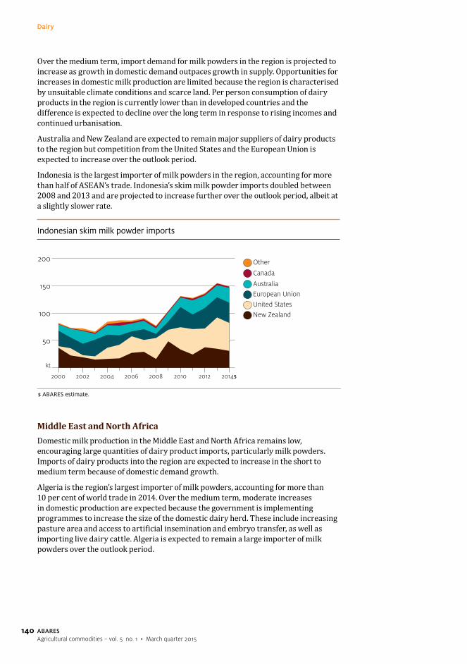
140
Dairy
ABARESAgricultural commodities – vol. 5 no. 1 • March quarter 2015
Over the medium term, import demand for milk powders in the region is projected to increase as growth in domestic demand outpaces growth in supply. Opportunities for increases in domestic milk production are limited because the region is characterised by unsuitable climate conditions and scarce land. Per person consumption of dairy products in the region is currently lower than in developed countries and the difference is expected to decline over the long term in response to rising incomes and continued urbanisation.
Australia and New Zealand are expected to remain major suppliers of dairy products to the region but competition from the United States and the European Union is expected to increase over the outlook period.
Indonesia is the largest importer of milk powders in the region, accounting for more than half of ASEAN’s trade. Indonesia’s skim milk powder imports doubled between 2008 and 2013 and are projected to increase further over the outlook period, albeit at a slightly slower rate.
Indonesian skim milk powder imports
kt
Other
Canada
AustraliaEuropean UnionUnited StatesNew Zealand
50
100
150
200
s ABARES estimate.
2014s2012201020082006200420022000
Middle East and North AfricaDomestic milk production in the Middle East and North Africa remains low, encouraging large quantities of dairy product imports, particularly milk powders. Imports of dairy products into the region are expected to increase in the short to medium term because of domestic demand growth.
Algeria is the region’s largest importer of milk powders, accounting for more than 10 per cent of world trade in 2014. Over the medium term, moderate increases in domestic production are expected because the government is implementing programmes to increase the size of the domestic dairy herd. These include increasing pasture area and access to artificial insemination and embryo transfer, as well as importing live dairy cattle. Algeria is expected to remain a large importer of milk powders over the outlook period.

141
Dairy
ABARESAgricultural commodities – vol. 5 no. 1 • March quarter 2015
JapanJapan’s cheese imports declined by almost 3 per cent in 2014 as a result of high import prices early in the year. Imports of cheese are expected to increase by 2 per cent in 2015 as a result of lower world prices and strong domestic demand. Over the medium term, Japan is expected to remain a large market for cheese, with Australia continuing to be a key supplier.
Prospects for the Australian dairy industryThe Australian farmgate price of milk is forecast to average 46.0 cents a litre in 2015–16, a 5 per cent increase over the forecast 2014–15 farmgate price of 44.0 cents a litre. The forecast rise reflects an assumed depreciation of the Australian dollar and forecast higher world dairy product prices.
Over the medium term, the Australian farmgate milk price is projected to increase moderately in real terms before easing in the latter half of the projection period in response to declining world dairy product prices. Farmgate milk prices are projected to average about 5 per cent higher in real terms over the outlook period than for the five years to 2013–14.
Australian milk production and farmgate price
Manufacturing milk
Market milk
ML2014–15Ac/L
Farmgate milk price (right axis)
2 000
4 000
6 000
8 000
10 000
12 000
10
20
30
40
50
60
f ABARES forecast. z ABARES projection.
2019–20z
2017–18z
2015–16f
2013–14
2011–12
2009–10
2007–08
2005–06
Milk productionAustralian milk production is forecast to increase by 2 per cent to 9.6 billion litres in 2015–16 following a forecast increase of 2 per cent in 2014–15. Assuming average seasonal conditions, dairy farmers in the southern export-oriented regions are expected to drive production growth. Increases in production will mostly reflect improvements in the milk yield per cow as dairy cow numbers are expected to remain largely unchanged. In the dairying regions more focused on the domestic drinking milk market, such as Queensland and Western Australia, production is expected to remain largely unchanged in 2015–16.

142
Dairy
ABARESAgricultural commodities – vol. 5 no. 1 • March quarter 2015
Over the medium term, milk production is projected to increase to around 10.1 billion litres. Increases in milk yields are expected to be the major driver behind the increase in production over the outlook period. The average milk yield per cow is projected to rise by 7 per cent over the five years to 2019–20, largely as a result of improved herd genetics, pasture management and farming technology.
The number of dairy cows is projected to rise in the first half of the outlook period as world dairy prices increase, reaching 1.71 million head in 2016–17. In the second half of the outlook period, declining world dairy prices are expected to reverse this trend, resulting in a slight decline in the dairy herd.
Australian exportsThe total value of Australian dairy exports is forecast to rise by 8 per cent in 2015–16 to $2.4 billion. This increase reflects an assumed depreciation of the Australian dollar, an increase in world dairy product prices and a forecast increase in export volumes. This follows a forecast 20 per cent fall in the value of dairy exports in 2014–15 to around $2.2 billion.
Over the medium term, Australia’s dairy export earnings are projected to increase, reaching as high as $2.5 billion (in 2014–15 dollars) in 2017–18. At the end of the outlook period, export earnings are projected to fall slightly in real terms because world dairy product prices are projected to decline.
In November 2014 the Australian Government announced the conclusion of the China–Australia Free Trade Agreement negotiations. Under the agreement, tariffs on imports of all Australian dairy products will be phased out over periods ranging between four and 11 years, depending on the product. Products with the most rapid tariff elimination include infant formula, casein, ice-cream, lactose and milk albumins, all of which will have tariffs eliminated over four years. The agreement is expected to increase the competitiveness of Australia’s dairy exports to China. However, over the medium term, the tariff rates applied to imports of Australian dairy products will continue to be higher than those applied to New Zealand dairy products. New Zealand dairy products have been subject to decreasing tariff rates in China since the New Zealand–China Free Trade Agreement came into effect in 2008.
Australian dairy exports, 2013–14
kt
Rest of world
Other AsiaChina
ButterWhole milkpowder
Skim milkpowder
Cheese
20
40
60
80
100
120
140
160

143
Dairy
ABARESAgricultural commodities – vol. 5 no. 1 • March quarter 2015
Outlook for dairy
unit 2012–13 2013–14 2014–15 f 2015–16 f 2016–17 z 2017–18 z 2018–19 z 2019–20 zunit 2012 13 2013 14 2014 15 f 2015 16 f 2016 17 z 2017 18 z 2018 19 z 2019 20 z
WorldWorldIndicative priceIndicative priceButter– nominal US$/t 3 727 4 498 3 525 3 713 3 885 3 982 4 026 4 014 nominal US$/t 3 727 4 498 3 525 3 713 3 885 3 982 4 026 4 014– real a US$/t 3 852 4 581 3 525 3 628 3 703 3 703 3 653 3 553 real a US$/t 3 852 4 581 3 525 3 628 3 703 3 703 3 653 3 553Skim milk powderSkim milk powder
l $/– nominal US$/t 3 731 4 513 2 775 3 022 3 255 3 390 3 309 3 279$/– real a US$/t 3 856 4 596 2 775 2 952 3 102 3 152 3 002 2 902US$/t 3 856 4 596 2 775 2 952 3 102 3 152 3 002 2 902Cheesenominal US$/t 4 150 4 817 3 950 4 200 4 357 4 493 4 522 4 466
Cheese– nominal US$/t 4 150 4 817 3 950 4 200 4 357 4 493 4 522 4 466real a US$/ 4 289 4 906 3 950 4 103 4 153 4 178 4 103 3 953– real a US$/t 4 289 4 906 3 950 4 103 4 153 4 178 4 103 3 953
AustraliaCow numbers b ’000 1 688 1 690 1 693 1 700 1 710 1 705 1 702 1 698AustraliaCow numbers b 000 1 688 1 690 1 693 1 700 1 710 1 705 1 702 1 698Milk yields L/cow 5 450 5 467 5 555 5 641 5 711 5 836 5 890 5 931Milk yields L/cow 5 450 5 467 5 555 5 641 5 711 5 836 5 890 5 931P d tiProductionTotal milk ML 9 201 9 239 9 405 9 590 9 765 9 950 10 025 10 070Total milk ML 9 201 9 239 9 405 9 590 9 765 9 950 10 025 10 070– Market sales ML 2 452 2 448 2 502 2 541 2 571 2 602 2 633 2 662– Market sales ML 2 452 2 448 2 502 2 541 2 571 2 602 2 633 2 662– Manufacturing ML 6 749 6 791 6 903 7 049 7 194 7 348 7 392 7 408– Manufacturing ML 6 749 6 791 6 903 7 049 7 194 7 348 7 392 7 408B kt 118 116 117 119 121 122 123 123Butter c kt 118 116 117 119 121 122 123 123Cheese kt 338 311 330 335 338 340 342 343Cheese kt 338 311 330 335 338 340 342 343Skim milk powder kt 224 211 220 224 227 230 232 234Skim milk powder kt 224 211 220 224 227 230 232 234Whole milk powder kt 109 126 117 120 124 127 129 130Whole milk powder kt 109 126 117 120 124 127 129 130F t ilk iFarmgate milk price– nominal Ac/L 40.2 51.2 44.0 46.0 49.8 53.3 54.2 55.1 nominal Ac/L 40.2 51.2 44.0 46.0 49.8 53.3 54.2 55.1– real d Ac/L 42.3 52.5 44.0 44.9 47.4 49.5 49.1 48.7 real d Ac/L 42.3 52.5 44.0 44.9 47.4 49.5 49.1 48.7Export volumeB kt 54 49 45 46 49 50 51 51Export volumeButter c kt 54 49 45 46 49 50 51 51Cheese kt 174 151 155 156 158 160 161 161CheeseSkim milk powder kt 147 143 148 153 158 162 166 169Skim milk powder kt 147 143 148 153 158 162 166 169Whole milk powder kt 87 94 85 86 89 91 92 93Whole milk powder kt 87 94 85 86 89 91 92 93E t lExport value– nominal A$m 2 232 2 725 2 195 2 378 2 572 2 721 2 745 2 745 nominal A$m 3 7 5 95 378 57 7 745 745– real d A$m 2 349 2 792 2 195 2 320 2 448 2 527 2 487 2 426 real d A$m 2 349 2 792 2 195 2 320 2 448 2 527 2 487 2 426a In 2014 15 US dollars b At 30 June c Includes the butter equivalent of butter oil butter concentrate ghee and dry butterfata In 2014–15 US dollars. b At 30 June. c Includes the butter equivalent of butter oil, butter concentrate, ghee and dry butterfat. d l d ll f fd In 2014–15 Australian dollars. f ABARES forecast. s ABARES estimate. z ABARES projection.p jSources: ABARES; Australian Bureau of Statistics; Dairy Australia, MelbourneSources: ABARES; Australian Bureau of Statistics; Dairy Australia, Melbourne

144
Dairy
ABARESAgricultural commodities – vol. 5 no. 1 • March quarter 2015
145
Dairy
ABARESAgricultural commodities – vol. 5 no. 1 • March quarter 2015
Fisheries

146 ABARESAgricultural commodities – vol. 5 no. 1 • March quarter 2015
FisheriesOutlook to 2019–20
Kasia Mazur, Robert Curtotti and Maggie Skirtun
• The gross value of Australia’s fisheries production is forecast to increase by 4.3 per cent in 2015–16 to $2.7 billion.
• Over the medium term to 2019–20, the real value of Australian fisheries production is projected to increase by 1.7 per cent. An expansion in the value of salmonid production will contribute most of the growth over this period.
• Over the medium term, the value of export earnings is projected to remain stable at around $1.4 billion (in real terms).
World fisheries consumption, production, trade and prices
ConsumptionGlobal seafood consumption has more than quadrupled in the past half century, from 28 million tonnes (9 kilograms per person) in 1961 to 136 million tonnes (19.2 kilograms per person) in 2012 (FAO 2014a). This growth has been faster than the aggregate of other human protein sources. As a result, the share of seafood in total animal protein supply for human consumption increased from 14 per cent to 17 per cent over this period. Most of the growth in per person seafood consumption has been in China, where per person consumption increased almost eightfold, from 4.3 kilograms in 1961 to 33.5 kilograms in 2011. Per person seafood consumption in developing countries (excluding China) more than doubled over the same period, from 5.6 kilograms in 1961 to 13 kilograms in 2011. The increase in per person seafood consumption in developed countries has been much slower. It rose by 35 per cent, from 17 kilograms to 23 kilograms, during the same period.
Seafood is consumed differently in developed and developing countries. In developed countries most seafood (55 per cent) is supplied to consumers frozen, and a further 27 per cent is supplied canned. In developing countries seafood is usually purchased fresh from wet markets; 54 per cent is supplied fresh. However, in developing countries, frozen products are increasing their share of the seafood consumption mix.

147
Fisheries
ABARESAgricultural commodities – vol. 5 no. 1 • March quarter 2015
Seafood consumption, by product type and region, 2001 and 2012
%
Canned
Prepared and preservedFrozen
Fresh
20
40
60
80
100
Developing2012
Developing2001
Developed2012
Developed2001
Source: FAO 2014a
Seafood production, trade and consumption, by region, 2011
Countries ProductionNon-food
uses Imports ExportsFood
supply Population
Annual per person
supply
Million tonnes in live weight Millions Kg/person
World 156.0 25.4 45.3 44.5 132.1 6 998.0 18.9
Developed
countries 29.0 5.7 27.4 19.2 31.8 1 383.8 23.0
Developing
countries 115.0 18.4 17.0 24.0 89.9 4 756.0 18.9
Developing
countries
(excluding China) 60.6 14.4 13.4 15.7 44 3 387.6 13.0
Least developed 11.9 1.2 0.8 1.3 10.3 858.2 12.0
Canada 1.1 0.1 0.6 0.9 0.8 34.5 22.3
United States 5.6 1.4 4.9 2.2 6.8 314.9 21.7
Australia 0.2 0.1 0.5 0.1 0.6 22.7 26.2 a
New Zealand 0.5 0.1 0.1 0.5 0.1 4.4 25.8
Japan 4.3 1.1 3.9 0.5 6.6 127.3 51.7
China 54.4 4.0 3.6 8.3 45.9 1 368.4 33.5
a ABARES estimates Australia’s apparent consumption of seafood for 2012–13 at 15 kilograms per person (edible weight equivalent) (Stephan & Hobsbawn 2014). This differs from the consumption estimate of the Food and Agriculture Organization (FAO) of the United Nations because the FAO estimates per person consumption on a live weight equivalent basis. Source: FAO 2014a

148
Fisheries
ABARESAgricultural commodities – vol. 5 no. 1 • March quarter 2015
The OECD–FAO Agricultural outlook 2014–23 estimates that seafood consumption will continue to grow over the next decade to around 20.9 kilograms per person (OECD–FAO 2014). Most of the increase will be in the Asian region, particularly China.
ProductionWorld fisheries production (edible and non-edible) increased by 1.4 per cent (2 million tonnes) in 2012 to 158 million tonnes. Aquaculture production continues to contribute most of the growth in global fisheries production (in volume terms) and reached a production value of US$138 billion in 2012. OECD–FAO (2014) estimates that by 2023 world fisheries production will rise to 186 million tonnes, with aquaculture production contributing to most of this growth.
Fisheries production from wild-catch and aquaculture, 1950 to 2012
Mt
Aquaculture
Wild-catch
30
60
90
120
150
180
20122006200019941988198219761970196419581952
Source: FAO 2014a
Most growth in world aquaculture production has occurred since 1992, with production increasing from 15 million tonnes (15 per cent of world production) to 67 million tonnes (42 per cent) from 1992 to 2012. Over this period aquaculture production was important in meeting increased global demand for seafood. Around 88 per cent of world edible aquaculture production is supplied from the Asian region, with China the single largest aquaculture producer. In 2012 China produced 41 million tonnes (US$66 billion) of aquaculture products, accounting for 62 per cent of global aquaculture production in volume terms and 48 per cent in value terms (FAO 2014a). Other large aquaculture producers include India, Vietnam and Indonesia. OECD–FAO (2014) estimates that by 2023 world aquaculture production will rise to 92 million tonnes, contributing almost half (49 per cent) of global production.
Wild-catch production has been relatively stable since the late 1980s, with an annual catch of around 90 million tonnes. Most wild-catch production (87 per cent) comes from marine waters, with seven countries accounting for 50 per cent of the total marine catch. In 2012 China produced 16.2 million tonnes of fisheries products, accounting for 18 per cent of world marine catch fisheries. Indonesia, the United States, India and Peru produced around 5 million tonnes each of wild-catch fisheries products in the same year. The Russian Federation and Japan produced around 4 million tonnes each. OECD–FAO (2014) estimates that by 2023 world wild-catch production will be around 95 million tonnes.
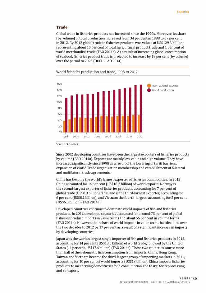
149
Fisheries
ABARESAgricultural commodities – vol. 5 no. 1 • March quarter 2015
TradeGlobal trade in fisheries products has increased since the 1990s. Moreover, its share (by volume) of total production increased from 34 per cent in 1998 to 37 per cent in 2012. By 2012 global trade in fisheries products was valued at US$129.3 billion, representing about 10 per cent of total agricultural product trade and 1 per cent of world merchandise trade (FAO 2014b). As a result of increasing global consumption of seafood, fisheries product trade is projected to increase by 18 per cent (by volume) over the period to 2023 (OECD–FAO 2014).
World fisheries production and trade, 1998 to 2012
World productionInternational exports
Mt
20
40
60
80
100
120
140
160
20122010200820062004200220001998
Source: FAO 2014a
Since 2002 developing countries have been the largest exporters of fisheries products by volume (FAO 2014a). Exports are mainly low value and high volume. They have increased significantly since 1998 as a result of the lowering of tariff barriers, expansion of World Trade Organization membership and establishment of bilateral and multilateral trade agreements.
China has become the world’s largest exporter of fisheries commodities. In 2012 China accounted for 14 per cent (US$18.2 billion) of world exports. Norway is the second-largest exporter of fisheries products, accounting for 7 per cent of global trade (US$8.9 billion). Thailand is the third-largest exporter, accounting for 6 per cent (US$8.1 billion), and Vietnam the fourth-largest, accounting for 5 per cent (US$6.3 billion) (FAO 2014a).
Developed countries continue to dominate world imports of fish and fisheries products. In 2012 developed countries accounted for around 73 per cent of global fisheries product imports in value terms and about 55 per cent in volume terms (FAO 2014b). However, their share of world imports in value terms has declined over the two decades to 2012 by 17 per cent as a result of a significant increase in imports by developing countries.
Japan was the world’s largest single importer of fish and fisheries products in 2012, accounting for 14 per cent (US$18.0 billion) of world trade, followed by the United States (14 per cent, US$17.6 billion) (FAO 2014a). These two countries source more than half of their domestic fish consumption from imports. China, Hong Kong, Taiwan and Vietnam became the third-largest group of importing markets in 2011, accounting for 10 per cent of world imports (US$13 billion). China imports fisheries products to meet rising domestic seafood consumption and to use for reprocessing and re-export.

150
Fisheries
ABARESAgricultural commodities – vol. 5 no. 1 • March quarter 2015
The OECD Western Europe is the largest single market for imported fish and fisheries products, accounting for 35 per cent (US$45.5 billion) of total world imports (FAO 2014a). The most traded fisheries commodity (by value) was shrimp in 2012, accounting for 15 per cent of the total value of internationally traded fisheries products (FAO 2014b).
Key importing regions, share of world trade, 2004 and 2012
OECD Western Europe 39%
United States 16%
China Vietnam region 8%
Japan 19%
OECD Western Europe 35%
United States 14%
China Vietnam region 10%
Japan 14%
2004
2012
Other 18%
Other 27%
Note: China Vietnam region includes China, Hong Kong, Taiwan and Vietnam. OECD Western Europe includes Austria, Belgium, Denmark, Finland, France, Germany, Greece, Iceland, Ireland, Italy, Luxembourg, the Netherlands, Norway, Portugal, Spain, Sweden, Switzerland, the United Kingdom.Sources: FAO 2008, 2014a
PricesGlobally, the price of fisheries products was steady in real terms from 1990 to 2002. Since then prices have increased significantly. The FAO Fish Price Index indicates a strong increase, from 90 in early 2002 to a record high of 160 in October 2014. This increase was mainly a result of a rise in prices for farmed species—particularly shrimp, some wild species such as cod and some pelagic species (FAO 2014b). OECD–FAO (2014) forecasts a slight decline in prices (in real terms) from 2014 to 2023.

151
Fisheries
ABARESAgricultural commodities – vol. 5 no. 1 • March quarter 2015
FAO Fish Price Index, 1990 to 2014
30
2002–04=100
60
90
120
150
180
201420112008200520021999199619931990
Source: FAO 2014b
Australian fisheries consumption, production and trade
ConsumptionAustralia’s apparent consumption of seafood increased on average by 1.3 per cent annually over the period 2003–04 to 2013–14, reaching 351 000 tonnes by 2013–14. Apparent consumption of seafood per person (edible equivalent) remained stable over this period, at around 15 kilograms per person. Most consumption growth is attributed to increased population.
Increased imports met most of the increase in seafood consumption. Imports increased on average by 2.4 per cent annually over this period. From 2003–04 to 2013–14, imports of prepared and preserved fish (mostly canned tuna, frozen fish products and prepared and preserved prawns) increased significantly. In 2013–14 imports contributed around 68 per cent of Australia’s total apparent consumption of seafood, up from 61 per cent in 2003–04.
Australian apparent seafood consumption by source, 2003–04 to 2013–14
kt
Domestic supplied
Imported
100
200
300
400
2013–14s
2011–12
2009–10
2007–08
2005–06
2003–04
s ABARES estimate. Source: Stephan & Hobsbawn 2014

152
Fisheries
ABARESAgricultural commodities – vol. 5 no. 1 • March quarter 2015
ProductionThe gross value of Australia’s fisheries production declined over the period 2003–04 to 2010–11, before rising from 2011–12 to 2013–14. Most of the decline to 2010–11 was driven by an appreciation of the Australian dollar exchange rate, a rise in competition from rising world aquaculture production and more conservative management settings in the wild-catch sector. More recently, growth in the production value of rock lobster, salmonids and prawns has supported growth in gross value of production (GVP).
In 2013–14 it is estimated that the GVP from fisheries products rose by 7 per cent ($174 million) to $2.6 billion. Contributing to the increase in GVP was an increase in the value of rock lobster production (rising by 20 per cent; $92 million), prawn production (30 per cent; $82 million) and salmonid production (9 per cent; $45 million).
From 2003–04 to 2013–14, the volume of seafood production declined by 8 per cent (21 019 tonnes) to 228 556 tonnes, while Australia’s fisheries GVP decreased by 12 per cent ($356 million) in real terms to $2.6 billion. Most of the decline is attributable to a significant reduction (25 per cent) in the combined value of tuna, prawns, rock lobster and abalone. Together, these four species contributed 47 per cent of Australia’s fisheries GVP in 2013–14, compared with 57 per cent in 2003–04. The main driver of this decline was a reduction in production volume of wild-catch of these species and in prices for abalone, prawns and tuna. From 2003–04 to 2013–14, the real GVP of wild-catch production decreased by 24 per cent ($484 million) in real terms. The largest declines were in prawns ($137 million), abalone ($113 million), rock lobster ($68 million) and tuna ($31 million). Wild-catch production declined from 215 187 tonnes to 153 228 tonnes over the same period.
Real gross value of production of key species, 2003–04 to 2013–14
OtherTunaAbalonePrawnsRock lobsterSalmonids
s ABARES estimate. Source: Stephan & Hobsbawn 2014
2013–14s
2011–12
2009–10
2007–08
2005–06
2003–04
2014–15$m
500
1 000
1 500
2 000
2 500
3 000
The volume of aquaculture production almost doubled over the period 2003–04 to 2013–14, in contrast to the significant decline in the wild-catch sector. As a result, aquaculture’s share of production grew from 17 per cent in 2003–04 to 34 per cent in 2013–14. The growth of the aquaculture sector in Australia was driven by a strong increase in production of salmonids. Since 2003–04 the volume of salmonid production more than doubled. Because of increasing prices the value of production

153
Fisheries
ABARESAgricultural commodities – vol. 5 no. 1 • March quarter 2015
increased at a faster rate. In 2013–14 salmonids accounted for 50 per cent in value terms and 52 per cent in volume terms of total Australian aquaculture production. The second most valuable aquaculture species is southern bluefin tuna. In 2013–14 Australia produced 7 800 tonnes with an estimated production value of $124 million.
Real gross value of production by sector, 2003–04 to 2013–14
Aquaculture
Commonwealth wild-catch
State wild-catch
500
1 000
1 500
2 000
2 500
3 000
s ABARES estimate. Note: Aquaculture total has been adjusted to exclude southern blue�n tuna caught in the Commonwealth SouthernBlue�n Tuna Fishery and introduced into farms in South Australia. This avoids double counting.Source: Stephan & Hobsbawn 2014
2013–14s
2011–12
2009–10
2007–08
2005–06
2003–04
2014–15$m
Average prices of key Australian species
2014–15$/kg
Abalone
Rock lobsterTuna PrawnsSalmonids
10
20
30
40
50
60
s ABARES estimate. Source: Stephan & Hobsbawn 2014
2013–14s
2011–12
2009–10
2007–08
2005–06
2003–04
TradeAustralia produces only about 0.2 per cent of global seafood. Despite this, it is a significant exporter of high value fisheries commodities and export earnings accounted for 49 per cent of total Australian production value in 2013–14. Australia imports a large proportion of domestic consumption requirements (68 per cent) and is a net importer of fisheries products in value terms.

154
Fisheries
ABARESAgricultural commodities – vol. 5 no. 1 • March quarter 2015
The value of Australian exports declined in real terms from 2003–04 ($2.2 billion) to 2013–14 ($1.3 billion). Most of the decline in export earnings occurred between 2003–04 and 2009–10, following the strong appreciation of the Australian dollar against the Japanese yen and the US dollar. This led to a decline in unit prices (particularly for prawns, tuna and abalone) and declines in production volume of rock lobster, prawns, tuna and abalone. In 2013–14 it is estimated that export earnings from fisheries products rose by 11 per cent ($129 million) to $1.3 billion.
Export and import values of fish products, 2003–04 to 2013–14
Exports
2014–15$m
Imports
500
1 000
1 500
2 000
2 500
2013–14
2011–12
2009–10
2007–08
2005–06
2003–04
Source: Stephan & Hobsbawn 2014
Australian main export products share, 2003–04 ($ 2 110 million) and 2013–14 ($1 267 million)
Pearls 19%Tuna 16%
Other 15%
Abalone 14%
Prawns 10%
Rock lobster 26%
Pearls 11%Tuna 10%
Other 13%
Abalone 13%
Prawns 8%
Rock lobster 45%
2003–04
2013–14
Source: Stephan & Hobsbawn 2014

155
Fisheries
ABARESAgricultural commodities – vol. 5 no. 1 • March quarter 2015
Australian main import products share, 2003–04 ($ 1 411 million) and 2013–14 ($1 944 million)
Prepared or preserved prawns 4%Other 37%
Frozen prawns 17%
Frozen �sh 21%
Prepared or preserved �sh 21%
2003–04
Prepared or preserved prawns 8%Other 34%
Frozen prawns 17%
Frozen �sh 15%
Prepared or preserved �sh 26%
2013–14
Source: Stephan & Hobsbawn 2014
Volume and value of Australian fisheries products exports
Volume (tonnes) Value (millions 2014–15 dollars)
Commodities 2003–04 2013–14 % change 2003–04 2013–14 % change
Rock lobster 13 453 7 966 –41 545 573 5
Prawns 9 397 7 055 –25 205 98 –52
Abalone 4 909 2 742 –44 303 165 –46
Tuna 12 813 11 000 –14 349 132 –62
Pearls na na na 397 140 –65
na Not applicable. Source: Stephan & Hobsbawn 2014

156
Fisheries
ABARESAgricultural commodities – vol. 5 no. 1 • March quarter 2015
In 2013–14 the main Australian fisheries export destinations were, in export value terms, Hong Kong, Japan, the United States, Taiwan and Vietnam. These countries accounted for 84 per cent of total Australian seafood exports in 2013–14.
Over the decade to 2013–14, China, Hong Kong, Taiwan and Vietnam have emerged as a key group of markets for Australia’s seafood exports. Japan was the largest market for Australian seafood exports in 2003–04, but exports to Japan have declined by almost 62 per cent in value terms since then. China has emerged as the largest destination for seafood from Australia. It receives much of its Australian seafood from re-exports via Hong Kong and Vietnam. Japan is the largest market for tuna. It imports more than 90 per cent of all tuna exported from Australia.
Major export destination markets for fisheries products, 2003–04 ($2 110 million in 2014–15 dollars) and 2013–14 ($1 267 million)
Other 18%
United States 9%
China Vietnam region 41%
Japan 32%
Other 14%
United States 3%
China Vietnam region 66%
Japan 17%
2003–04
2013–14
Note: China Vietnam region includes China, Hong Kong, Taiwan and Vietnam. Source: Stephan & Hobsbawn 2014
Australia imports a range of fish and fisheries products, mainly from Thailand, New Zealand, China and Vietnam. These countries together accounted for 61 per cent of total fisheries product imports in 2013–14. A large proportion of imported fisheries product from Thailand is canned tuna. The key imported products from New Zealand are frozen and fresh fish, and from China farmed prawns and frozen squid. The largest commodity product groups imported from Vietnam are frozen fish and prepared and preserved prawns. Over the decade to 2013–14, the real value of Australian imports ranged between $1.41 billion and $1.9 billion and, in 2013–14, was $2 billion.

157
Fisheries
ABARESAgricultural commodities – vol. 5 no. 1 • March quarter 2015
Volume and value of Australian fisheries products imports
Volume (tonnes) Value (millions in 2014–15 dollars)
Products 2003–04 2013–14 % change 2003–04 2013–14 % change
Prepared or
preserved fish 70 994 87 400 23 303 504 67
Frozen fish fillets 58 242 55 588 –5 304 304 0
Fresh, chilled or
frozen prawns 18 865 25 863 37 235 330 41
Prepared or
preserved prawns 5 584 12 808 129 56 150 168
Australian fisheries and aquaculture production medium-term outlook (major products)The gross value of Australia’s fisheries production is forecast to increase by 4 per cent ($110 million) in 2015–16, with the fisheries GVP to reach almost $2.7 billion. This growth follows a forecast 1 per cent increase in growth in 2014–15. In 2015–16 export earnings from fisheries products are forecast to increase by 8.1 per cent ($109 million) to $1.5 billion.
Given the large export focus of Australia’s seafood sector, GVP and export earnings tend to be affected by exchange rate movements. From 2001–02 to 2012–13, the Australian dollar appreciated significantly against the US dollar and on a trade-weighted basis. The appreciation of the Australian dollar over this period resulted in lower competitiveness of Australian product overseas and an increase in the competitiveness of imports in the domestic market. The high value of the Australian dollar over this period contributed to a decline in the value of production and lower export earnings.
In 2013–14 the Australian dollar began depreciating against major currencies, contributing to the higher value of production and higher export earnings in 2013–14. It is assumed that Australia’s exchange rate will continue to depreciate in 2015–16 (by a further 15 per cent against the US dollar and 10 per cent on a trade-weighted basis), supporting growth in GVP and export earnings. It is assumed in this set of forecasts that exchange rates will remain more stable for the remainder of the period to 2019–20.
Over the medium term the value of production is projected to increase by 1.7 per cent to reach $2.7 billion (in real terms) by 2019–20. Export earnings are projected to remain at around $1.4 billion (in real terms) over the period.

158
Fisheries
ABARESAgricultural commodities – vol. 5 no. 1 • March quarter 2015
Real value of fisheries production, export and the Australian–US dollar exchange rate
Gross value of production
2014–15$b
A$/US$
Export value
Exchange rate(right axis)
z ABARES projection.
0.5
1.0
1.5
2.0
2.5
3.0
3.5
0.3
0.6
0.9
1.2
1.5
1.8
2.1
2019–20z
2016–17z
2013–14
2010–11
2007–08
2004–05
PrawnsIn 2015–16 the value of prawn production is forecast to increase by 8.3 per cent ($28 million) to reach $367 million. Exports of prawn products are also forecast to rise by 9.1 per cent to reach $105 million in the same year.
Prawn production declined over the decade to 2012–13 by 20 per cent to 21 145 tonnes. Most of this decline is attributed to lower production from Australia’s wild-caught prawn fisheries, where production declined by 5 719 tonnes to 17 403 tonnes. The decline was largely the result of a decline in production from the Commonwealth Northern Prawn Fishery, the Torres Strait Prawn Fishery and the prawn fisheries of Western Australia, Queensland and New South Wales. Growth in prawn aquaculture production offset some of the decline in wild caught production, growing by 11 per cent to reach 3 742 tonnes by 2012–13. In 2012–13 Queensland produced 3 519 tonnes of aquaculture prawns, accounting for 94 per cent of Australia’s prawn aquaculture production. Wild-caught prawn production accounted for 82 per cent of Australia’s total prawn production in 2012–13.
The value of production also declined significantly over the decade to 2012–13, by 42 per cent in real terms to $277 million. This decline reflects lower production volumes and lower average beach prices for the major prawn species—tiger, king and endeavour prawns. Lower prices mainly reflect the negative impact of the high value of the Australian dollar on export unit values in the period and competition in the domestic market from imported farmed prawns from Asia.
In 2013–14 the value of prawn production increased by 30 per cent ($82 million) to reach $359 million. A better than average banana prawn season for the Commonwealth Northern Prawn Fishery in that year significantly increased the landed value of catch for that fishery. Over the medium term to 2019–20, it is projected that the real value of production of prawns and export earnings will decline by 8 per cent, to $328 million and $94 million, respectively.

159
Fisheries
ABARESAgricultural commodities – vol. 5 no. 1 • March quarter 2015
SalmonidsIn 2015–16 the volume of Australian salmonid production is forecast to expand by 2 300 tonnes, in part because of the planned industry expansion of salmonid production in Tasmania’s Macquarie Harbour. This follows a forecast expansion of production in 2014–15 of 3 500 tonnes. The forecast increase in production in these years follows significant expansion of salmonid production over the decade to 2013–14, from 16 686 tonnes in 2003–04 to 41 615 tonnes in 2013–14. Almost all of this growth is a result of the expansion of salmon aquaculture farms in Tasmania. Tasmania accounts for around 97 per cent of total salmonid production.
The value of production of salmonids tripled during the decade to 2013–14. It reached $542.5 million in that year, reflecting the significant increase in volume. Salmon is produced predominantly for the Australian domestic market. In 2013–14 the value of export was $17.4 million. Most salmon is exported in fresh or chilled form.
Over the medium term salmon production is projected to continue to grow, reflecting an anticipated expansion of production to 61.4 million tonnes in 2019–20. As a result, the value of production is projected to increase by 23 per cent over the medium term to $696 million (in 2014–15 dollars). In line with rising production, the export of salmonid products is projected to increase over the medium term $47 million by 2019–20. By then it is projected that 10 per cent of salmonid production will be exported. This will represent a rise from 4 per cent in 2013–14.
Rock lobsterIn 2015–16 it is forecast that Australia will produce 10 268 tonnes of rock lobster with a value of $598 million. Rock lobster is forecast to contribute approximately 22 per cent to the total value of fisheries production, representing the highest value for wild-catch species. Overseas market prices have been high recently, which has flowed through to domestic producers.
In the decade from 2003–04 to 2013–14, total rock lobster production volume fell by 49 per cent. In contrast, the value of rock lobster production is estimated to have increased by 3 per cent over the same period. In 2013–14 an international price shock affected rock lobster. The average domestic beach price increased from $42.75 in 2012–13 to $54.87 in 2013–14. This increased rock lobster production value by almost $100 million. Almost 60 per cent of Australia’s rock lobster production is in Western Australia. The other main rock lobster fisheries are in South Australia (estimated at 16 per cent of total catch in 2013–14), Tasmania (11 per cent), Queensland (7 per cent) and Commonwealth waters (4 per cent).
The decline in production volume of rock lobster in the period 2003–04 to 2013–14 has been driven by a 58 per cent reduction in catches from the Western Australian West Coast Rock Lobster Fishery. More than 74 per cent of the volume of rock lobster production is exported, mainly to Hong Kong and China.
The value of production and export is projected to increase over the medium term to $636 million and $697 million by 2019–20, respectively.

160
Fisheries
ABARESAgricultural commodities – vol. 5 no. 1 • March quarter 2015
AbaloneIn 2015–16 abalone production is expected to recover slightly, by 5 per cent, to 5 161 tonnes and generate around $163 million in revenue. This is forecast to be driven by improvements in wild-caught abalone landings in Tasmania and growing aquaculture production in Victoria and South Australia. The establishment of abalone farms in Western Australia is also forecast to contribute to this growth.
The abalone industry in Australia is predominantly export oriented. Between 2003–04 and 2011–12, exports constituted on average 68 per cent of production, in volume terms. However, this has fallen to a little above 50 per cent in the past few years. Historically, most of Australia’s abalone production has been harvested from wild-catch fisheries in Tasmania, Victoria and South Australia. However, over the decade to 2013–14, aquaculture production in these states expanded, with an estimated 17 per cent (843 tonnes) of total abalone production in 2013–14 sourced from aquaculture farms.
In December 2005, a virus was detected in two land-based abalone aquaculture farms and two offshore experimental farms in Victoria. The disease then spread to the western zone, and parts of the central zone, of the Victorian Abalone Fishery. This forced areas of the fishery to be closed and total allowable catch to be reduced. Measures were also put in place to try to prevent the spread of the disease to other parts of the fishery and across Bass Strait to Tasmania. Both price and total allowable catch fell, leading to a reduction in abalone production. A more recent outbreak of the disease in western Victoria was successfully contained, resulting in no major effect on total production volumes.
In the medium term, production is projected to increase to around 6 244 tonnes ($208 million, in nominal dollars) by 2019–20, with farmed abalone driving the growth and making up almost one-third of this production. In contrast, export earnings are projected to grow only moderately despite the assumed depreciation of the Australian dollar. The dampening effect comes predominantly from an increase in farmed abalone competition particularly into China, the largest export destination for Australian abalone.
ScallopsIn 2015–16 scallop production is forecast to improve slightly to 6 066 tonnes (value $14 million). The improvement in scallop production is based on forecast recovery in the Bass Strait zone contributing to increased catches in the Commonwealth Bass Strait Central Zone Scallop Fishery and the Tasmanian and Victorian scallop fisheries.
Unlike abalone, all Australian scallops are harvested from wild-catch fisheries. In volume terms, scallops have historically been the largest wild-caught mollusc species group produced, accounting for an average of 49 per cent of total wild-catch mollusc production from 2003–04 to 2010–11. However, in 2011–12 scallop production decreased, by 49 per cent (3 392 tonnes) to 3 563 tonnes. This was the result of deteriorating conditions for commercial scallops in the Bass Strait and a reduction in the harvest of Western Australian saucer scallops. Continually depleted stock levels coupled with the discovery of a toxic algae bloom reduced scallop production in the Bass Strait (Victorian, Tasmanian and Commonwealth waters) by 72 per cent or 1 466 tonnes in 2011–12, compared with 2010–11.

161
Fisheries
ABARESAgricultural commodities – vol. 5 no. 1 • March quarter 2015
In the same year, Western Australian scallop fisheries suffered a marine heatwave that killed off most of their scallop abundance and reduced scallop harvest from 3 060 tonnes to 158 tonnes. Since the marine heatwave in 2011–12, Western Australian scallop production has not recovered; 2014 was the third consecutive year that the two main scallop fisheries, Shark Bay and the Abrolhos Islands, were closed to commercial fishing. Small amounts of scallops are being caught in the South West Trawl Managed Fishery, around Rottnest Island, but scallop abundance remains low. In 2012–13 total scallop production almost doubled to 6 750 tonnes, owing to a tremendous season for the Queensland saucer scallop fishery. This is estimated to have declined to around 5 043 tonnes in 2013–14.
Over the medium term Australian scallop production is projected to vary as a result of fluctuations in the stock of this marine bivalve species. It is projected that catch will return to late 2000 levels of 7 138 tonnes by 2019–20, generating a revenue of $22 million, in nominal terms. Australian scallops are predominantly domestically consumed; only 12 per cent of scallops were exported, on average, between 2003–04 and 2013–14. However, with improvements in scallop production and an assumed depreciation in the exchange rate over the medium term, scallop export earnings are projected to increase by 24 per cent from $17 million in 2015–16 to $21 million in 2019–20 (in nominal values).
TunaIn 2015–16 the value of tuna production is forecast to increase by 10.5 per cent ($17 million) to $173 million. Exports of tuna products are also forecast to rise, by 9.4 per cent to reach $161 million in the same year.
The principal tuna species caught in value and volume terms is southern bluefin tuna, which is caught from Commonwealth waters using purse seine methods and then fattened in farms near Port Lincoln. The majority of Australia’s tuna production is exported mostly to the Japanese sashimi market. Over the decade to 2013–14, tuna production decreased by 22 per cent in volume terms to 11 498 tonnes and 47 per cent in value terms to $148.5 million (in real terms). In line with lower production, the value of exports also declined—by more than 50 per cent to $135.5 million.
Over the medium term world production of northern and southern bluefin tuna will be constrained by international quota limits. The global total allowable catch for southern bluefin tuna has increased for the 2015 season, with Australia’s allocation raised from 5 193 in 2014 to 5 665 tonnes. Despite this increase, growth in tuna GVP is expected to be constrained by a period of soft prices as a result of the assumed strength of the Japanese yen over this period. Over the medium term the value of tuna production is projected to decline, by 8 per cent to $155 million.
Short-term boost to profitability through lower fuel costs
Fuel prices and fishing costsFuel is a major cost for fishing businesses. ABARES surveys of key Commonwealth fisheries indicate that fuel costs range from 10 per cent to 41 per cent of the total cost of operating a vessel, depending on the fishery and main method of fishing used in the fishery (Skirtun, Stephan & Mazur 2014). In the Northern Prawn Fishery and the Torres Strait Prawn fishery (TSPF), the proportion was relatively high in 2011–12, at 27 per cent and 41 per cent, respectively. This reflects the longer distances travelled and the more fuel intensive fishing method used in these fisheries.

162
Fisheries
ABARESAgricultural commodities – vol. 5 no. 1 • March quarter 2015
Increases in world oil prices in recent years have caused diesel prices to increase, increasing costs to operators. The real average wholesale diesel price rose from 115 cents a litre in 2002–03 to 155 cents a litre in 2007–08. Fishers are entitled to a rebate on their fuel expense under the Energy Grants Credit Scheme. For claims made since early January 2006, the rebate is approximately 38 cents a litre. The price reflects the price paid per litre by fishers taking into account the diesel fuel rebate. Despite the decrease in the off-road diesel price after 2007–08, prices are still at relatively high levels.
Fuel costs as a percentage of total cash costs for selected Commonwealth fisheries/sectors
Fishery
2009–10 2010–11 2011–12
% change % change % change
Torres Strait Prawn Fishery na 41 41
Northern Prawn Fishery 26 25 27
Eastern Tuna and Billfish Fishery 13 14 na
Commonwealth Trawl Sector 16 16 na
Gillnet Hook and Trap Sector 11 12 na
na Not available. Note: Percentages are calculated from average fishery financial performance reported in the Australian fisheries economic indicator report (formerly the Australian fisheries surveys report). Average fishery financial performance reflects profit and loss statement for the (weighted) average boat for all business activities, including operation in other fisheries during the survey period.
Real average off-road diesel price, inclusive of farm rebates and subsidies but excluding GST, 2003–04 to 2014–15
2014–15Ac/L
20
40
60
80
100
120
140
2014–15p
2012–13
2010–11
2008–09
2006–07
2004–05
p ABARES preliminary estimates.
163
Fisheries
ABARESAgricultural commodities – vol. 5 no. 1 • March quarter 2015
The wholesale diesel price at the terminal gate declined sharply in the latter part of 2014 and into 2015. Movements in wholesale diesel prices are closely aligned with movements in international oil prices. The West Texas Intermediate price, a benchmark international crude oil price, declined by 44 per cent in the last six months of 2014, to around US$59 a barrel. While it is unclear whether recent lows in the international price of crude oil will continue over the medium term, the current price settings provide industry with a significant reprieve in fuel costs in the short term.
Trade liberalisation improves access for Australian seafood to key marketsRecent bilateral trade agreements between Australia and some of its key trading partners are likely to improve access for Australian seafood to key markets.
In late 2014, Australia and China concluded negotiations for a China–Australia Free Trade Agreement (ChAFTA). In value terms China is the world’s largest exporter (US$18.2 billion) and the fifth-largest importer (US$7.4 billion) of fisheries commodities (FAO 2014a). Australian direct seafood exports to China totalled $39.2 million in 2013–14—including edible fish products ($35.5 million) and non-edible ($3.6 million). However, most trade to China from Australia is indirect trade via re-exports from Hong Kong and Vietnam. Most of Australia’s rock lobster and abalone production is exported to China through direct and indirect re-exports. Other major commodities exported directly to China include prawns ($6.7 million) and crabs ($1.9 million) (Stephan & Hobsbawn 2014).
Implementation of ChAFTA will result in a progressive elimination of tariffs on Australian seafood exports to China, to be phased in over four years. Tariffs to be eliminated include the current 10 per cent to 14 per cent tariff on abalone; the 15 per cent tariff on rock lobster; the 12 per cent tariff on southern bluefin tuna, salmon, trout and swordfish; the 14 per cent tariff on crabs, oysters, scallops and mussels; and the up to 8 per cent tariff on prawn imports. Given that demand in China is growing continuously, the implementation of ChAFTA should lead to more direct trade with China and allow Australia to better compete with other seafood exporting nations.
The Japan–Australia Economic Partnership Agreement (JAEPA) entered into force on 15 January 2015. Japan is one of the largest consumers of fisheries products, with per person fish consumption of 52 kilograms in 2011. Japan is the second-largest importer of fish products worldwide (US$18 billion in 2012); imports account for over half of its domestic consumption. The main fish products imported by Japan are tuna, salmon, trout, shrimps. Japan is the world’s largest market for sashimi-grade tuna (FAO 2014a, 2014b).
Japan is an important market for Australian fish products—worth $219 million in 2012–13, with $192.1 million worth of edible products and $26.9 million of non-edible fish products. Almost all Australian production of tuna is exported to Japan, amounting to a value of $125.4 million. Most of the tuna exported to Japan is southern bluefin tuna, which is one of the most highly valued fish species for the Japanese sashimi market. The other major commodities exported to Japan include prawns ($23 million), abalone ($21 million) and salmonids ($8 million).
From early 2015, the JAEPA agreement eliminates tariffs of up to 9.6 per cent on lobsters, shrimps and prawns, abalone (fresh or preserved), oysters, crabs, fresh sea urchins, fish oils and some fish. Tariffs on tuna, Atlantic salmon, swordfish and marlin will be eliminated over 10 years.

164
Fisheries
ABARESAgricultural commodities – vol. 5 no. 1 • March quarter 2015
The Korea–Australia Free Trade Agreement (KAFTA) entered into force on 12 December 2014. The Republic of Korea is Asia’s fourth-largest economy, with a population of 50 million. Tariffs on most seafood products will be progressively reduced to zero through this agreement. KAFTA provides improved market access for Australian fish products by the immediate or phased elimination of tariffs. For example, the 20 per cent tariff applying to rock lobster imports will be removed after three years and the 10 per cent tariff on southern bluefin tuna will be removed after five years. This will provide further opportunity for Australia to export these products to Korea.
ReferencesFAO 2014a, Fishery and aquaculture statistics 2012, Food and Agriculture Organization of the United Nations, Rome.
FAO 2014b, The state of world fisheries and aquaculture 2014, Food and Agriculture Organization of the United Nations, Rome.
FAO 2008, Fishery and aquaculture statistics 2006, Food and Agriculture Organization of the United Nations, Rome.
OECD–FAO 2014, Agricultural outlook 2014–2023, OECD Publishing, Paris.
Skirtun, M, Stephan, M & Mazur, K 2014, Australian fisheries economic indicators report 2013: financial and economic performance of the Northern Prawn Fishery, Australian Bureau of Agricultural and Resource Economics, Canberra, April.
Stephan, M & Hobsbawn, P 2014, Australian fisheries and aquaculture statistics 2013, ABARES Fisheries Research and Development Corporation project 2010/208, Canberra, November.

165
Fisheries
ABARESAgricultural commodities – vol. 5 no. 1 • March quarter 2015
Outlook for fisheries products
2012–13 2013–14 s 2014–15 f 2015–16 f 2016–17 z 2017–18 z 2018–19 z 2019–20 z
$m $m $m $m $m $m $m $m
Tuna a 177 149 157 173 169 175 178 176– real b 186 152 157 169 161 162 161 155Salmonids 497 542 577 580 659 680 740 787– real b 523 556 577 565 627 632 671 696Other fish 441 466 438 437 445 448 445 443– real b 464 478 438 426 424 416 404 392Prawns 277 359 339 367 365 366 369 371– real b 292 368 339 358 347 340 334 328Rocklobster c 451 543 537 598 608 618 625 636– real b 475 556 537 583 579 574 566 562Abalone 190 160 163 153 158 166 171 178– real b 200 164 163 149 150 154 155 157Scallops 15 11 14 15 13 15 20 22– real b 15 12 14 14 12 14 18 20Other 334 324 353 366 364 376 398 403– real b 351 332 353 357 347 349 361 357Total 2 381 2 555 2 577 2 688 2 781 2 843 2 947 3 016– real b 2 506 2 617 2 577 2 622 2 647 2 640 2 670 2 666
Tuna b 163 136 147 161 157 162 165 163– real b 171 139 147 157 149 151 149 144Salmonids 25 17 28 31 38 41 48 53– real b 27 18 28 31 36 39 43 47Other fish 70 72 79 74 75 76 75 75– real b 74 74 79 72 71 70 68 66
frozen 51 99 97 105 105 105 106 107– real b 54 102 97 103 100 98 96 94
fresh chilled frozen or cooked 447 590 580 645 658 671 682 696– real b 471 605 580 629 627 624 618 615
live, fresh or chilled 80 74 77 80 87 87 85 90– real b 84 75 77 78 83 80 77 79 frozen or cooked 55 56 50 55 63 58 58 61– real b 58 57 50 53 60 54 52 54 prepared or preserved 52 41 41 48 57 55 58 60– real b 54 42 41 47 54 51 52 53Scallops 11 14 12 17 13 20 18 21– real b 11 14 12 17 12 18 17 19Other fisheries products 70 61 66 61 63 65 74 68– real b 74 63 66 60 60 61 67 61Total (excluding pearls) 1 024 1 160 1 177 1 278 1 315 1 340 1 368 1 395– real b 1 077 1 188 1 177 1 246 1 252 1 245 1 239 1 233Pearls 152 144 171 178 184 189 192 197– real b 159 148 171 174 176 176 174 174Total (including pearls) 1 175 1 304 1 347 1 456 1 499 1 529 1 560 1 591– real b 1 237 1 336 1 347 1 420 1 427 1 420 1 413 1 406
Fisheriesproductsoutlook
Gross value of fisheries production
Export value
Rocklobster
Abalone
a Exports of tuna landed in Australia. Excludes tuna transhipped at sea or captured under joint venture or bilateral agreements. b In 2014–15 Australian dollars. c Includes Queensland bugs. d Includes headless and whole prawns only. f ABARES forecast. s ABARES estimate. z ABARES projection.Sources: ABARES; Australian Bureau of Statistics
Prawns d

166
Fisheries
ABARESAgricultural commodities – vol. 5 no. 1 • March quarter 2015
167
Fisheries
ABARESAgricultural commodities – vol. 5 no. 1 • March quarter 2015
Farm performance

168 ABARESAgricultural commodities – vol. 5 no. 1 • March quarter 2015
Farm performance: broadacre and dairy farms, 2012–13 to 2014–15Peter Martin, Therese Thompson, Paul Phillips and Walter Shafron
• Incomes of broadacre farms have been relatively high in recent years compared with incomes recorded historically. Nationally, farm cash income increased from $110 270 in 2012–13 to $124 600 in 2013–14. In 2014–15 farm cash income is projected to decline to average $114 000 a farm. This is around 20 per cent above the 10-year average to 2013–14 of $94 500. However, major differences exist in average farm cash incomes across industries, states and regions.
• Farm cash incomes of Western Australian and South Australian broadacre farms are projected to decline in 2014–15 as a result of a reduction in winter grain production from the record production in 2013–14. Farm cash income in 2014–15 is projected to average $211 000 for Western Australian broadacre farms and $163 000 for South Australian broadacre farms. These projected incomes are around 30 per cent above the average for the decade ending 2013–14.
• Reduced grain production is also projected to lower average farm cash income in Victoria. Farm cash income in 2014–15 is projected to average $68 000 for Victorian broadacre farms, around 13 per cent below the average for the decade ending 2013–14.
• Average farm cash income is projected to increase in the Northern Territory because of higher cattle prices and high turn-off of beef cattle in 2014, including increased sale of beef cattle for live export.
• Incomes are also projected to rise in Queensland mainly because of higher beef cattle prices. Drought continued to affect Queensland broadacre farms in 2014, subduing crop and livestock production and maintaining high turn-off of cattle and sheep. Despite higher beef cattle prices, farm cash income is projected to increase only slightly to an average of $79 000 a farm in 2014–15. This is only a small increase from the $68 200 recorded in 2013–14 and is still around 10 per cent below the average for the decade ending 2013–14.
• Average farm cash income of New South Wales broadacre farms is projected to decline slightly compared with the previous year to average $106 000 a farm in 2014–15. Higher sheep, lamb and beef cattle prices and increased production of grain in central and southern regions offset further reductions in grain production in northern New South Wales as a result of prolonged drought.

169
Farm performance: broadacre and dairy farms, 2012–13 to 2014–15
ABARESAgricultural commodities – vol. 5 no. 1 • March quarter 2015
• Higher beef cattle prices have resulted in projected farm cash income of beef industry farms increasing nationally to average $63 000 a farm in 2014–15 despite a sharp reduction in numbers of beef cattle sold in the second half of 2014–15. Nevertheless, average beef industry farm cash income is projected to be around 3 per cent below the 10-year average to 2013–14.
• Grains industry farm cash income is projected to decline to average $225 000 a farm in 2014–15 as a result of reductions in winter crop production in all states because of lower grain yields. If realised, average grains industry farm cash income would still be about 14 per cent above the 10-year average to 2014–15.
• Farm cash income is projected to decline for dairy farms in most states except Queensland and Western Australia in 2014–15, as a result of lower farmgate milk prices and despite increased milk production. At the national level, average farm cash income of dairy farms is projected to decline from an average of $163 900 in 2012–13 to an average of $97 000 a farm in 2014–15.
• Farm business debt is estimated to have declined slightly for broadacre farms each year since 2009–10 as a result of a reduction in new borrowing and continued debt repayment. At the national level, broadacre debt is estimated to have remained largely unchanged during 2013–14 and averaged $512 500 a farm at 30 June 2014. Debt of farm businesses affected by drought in 2013–14 increased by an average of 5 per cent but declined by an average of 1 per cent for all other farms.
OverviewABARES Australian Agricultural and Grazing Industries Survey (AAGIS) projects an overall decline in average incomes of Australian broadacre farms in 2014–15. Reductions in grain production are projected to result in a decline in income for Victorian, Western Australian and South Australian farms. In New South Wales, taken as a whole, farm cash income is projected to decline only slightly compared with that recorded in 2013–14. In contrast, an increase is projected for income in Queensland and the Northern Territory, mainly as a result of higher beef cattle prices. In Tasmania higher beef cattle, sheep and lamb prices are projected to result in increases in farm incomes.
Financial pressure increased on farm businesses in several industries and regions during 2012–13 as a result of the combination of low beef cattle and milk prices, dry seasonal conditions, high farm debt and the erosion of farm equity through reductions in land values. Those most affected included the beef industry in northern Australia, grain producers in the Western Australian wheat belt and dairy farmers in western Victoria.
Higher farm incomes in 2013–14 reduced some pressure, particularly in Western Australia and the southern dairy industry. Pressure was also reduced more broadly by reduction in broadacre farm debt and a decline in interest rates. However, financial pressure continued in regions highly reliant on beef cattle production and in the northern New South Wales and Queensland regions subject to prolonged drought conditions.
In 2014–15 incomes are projected to increase for beef industry farms in all states as a result of higher cattle prices. The increase in income will reduce financial pressure in some regions but may have only a small effect in regions constrained by the reduced availability of saleable cattle after two years of high turn-off. Financial pressure is likely to continue in 2014–15 as herds and flocks are rebuilt. Further, incomes are projected to remain low for cropping farms that were subject to dry conditions well into 2014–15.

170
Farm performance: broadacre and dairy farms, 2012–13 to 2014–15
ABARESAgricultural commodities – vol. 5 no. 1 • March quarter 2015
Farm receipts
2013–14Average total cash receipts of broadacre farms increased by around 9 per cent in 2013–14 compared with 2012–13.
In 2013–14 average crop receipts increased by around 7 per cent as a result of increased winter grain production and higher wheat, oilseeds and pulse prices and despite low overall production of grain sorghum and other summer crops.
Large increases in beef cattle turn-off resulted in overall receipts for beef cattle rising despite a reduction of around 4 per cent in the average price received for beef cattle sold.
Higher prices for sheep and lambs and an increase in the number of sheep sold resulted in an increase of around 28 per cent in average sheep and lamb receipts a farm. Receipts from wool for broadacre farms increased slightly, with a small increase in wool production and slightly higher wool prices.
At the national level, receipts for dairy farms increased by around 29 per cent, on average, with higher milk prices in all states, compared with 2012–13. The largest increases in milk prices occurred in Victoria, Tasmania, South Australia and southern New South Wales. Milk production also increased slightly.
Box 1 Broadacre sector of Australian agricultureThe sector includes five industry types:
Wheat and other crops industry: specialised producers of cereal grains, coarse grains, pulses and oilseeds.
Mixed livestock–crops industry: properties engaged in producing sheep and/or beef cattle in conjunction with substantial activity in broadacre crops such as wheat, coarse grains, oilseeds and pulses.
Sheep industry: specialised producers of sheep and wool. Sheep industry farms account for only 30 per cent of Australia’s wool production. Most wool and sheep meat production occurs on mixed enterprise farms, particularly on mixed livestock–crop industry farms.
Beef industry: properties engaged mainly in running beef cattle, which currently account for around 65 per cent of Australia’s beef production. This industry includes many small farms.
Sheep–beef industry: properties engaged in running sheep and beef cattle. This industry includes many small farms.

171
Farm performance: broadacre and dairy farms, 2012–13 to 2014–15
ABARESAgricultural commodities – vol. 5 no. 1 • March quarter 2015
FIGURE 1 Farm cash receipts, broadacre industries
Other
2014–15$’000
Sheep and lamb receipts
y ABARES provisional estimate.
Wool
Beef cattleCrops
100
200
300
400
500
2014–15y
2011–12
2008–09
2005–06
2002–03
1999–2000
1996–97
2014–15Average total cash receipts a broadacre farms are projected to decrease by around 4 per cent in 2014–15 compared with 2013–14.
In 2014–15 average crop receipts are projected to decrease by around 10 per cent as a result of decreased winter grain production in all states resulting from lower grain yields and lower prices for wheat, oilseeds and pulses.
Higher average prices for beef cattle are expected to result in a rise in overall receipts for beef cattle. This is despite a sharp reduction in numbers of beef cattle sold in the second half of 2014–15.
Higher prices for sheep and lambs are projected to result in an increase of around 8 per cent in average sheep and lamb receipts a farm, despite a small decrease in the number of sheep sold. A small decline is expected in receipts from wool for broadacre farms, with a small reduction in wool production combined with slightly lower wool prices.
At the national level, compared with 2013–14, receipts of dairy farms are projected to decrease by around 9 per cent, on average, with higher milk production more than offset by the lower milk prices expected in most states.

172
Farm performance: broadacre and dairy farms, 2012–13 to 2014–15
ABARESAgricultural commodities – vol. 5 no. 1 • March quarter 2015
Farm costs
2013–14For broadacre farms, average total cash costs increased by 8 per cent in 2013–14 as expenditure increased across a wide range of farm inputs. The largest increases in expenditure were on fodder, fertiliser and purchases of sheep. Large reductions were recorded in expenditure on beef cattle purchase in the Northern Territory, Queensland, Victoria and Tasmania.
For dairy industry farms, fodder expenditure increased in most states as a result of drier seasonal conditions. Small increases were recorded in most other categories of farm cash costs, including interest payments as farm debt increased. Average total cash costs for the Australian dairy industry increased by 9 per cent in 2013–14 compared with 2012–13.
2014–15At the national level, average total cash costs per broadacre farm are projected to decline by around 2 per cent compared with 2013–14. Expenditure on fuel is projected to decline in all states as a result of lower fuel prices, and lower interest rates are projected to result in a small reduction in interest payments. Freight, handling and marketing costs are also projected to decline, resulting from harvest of a smaller winter grain crop and reduced turn-off of beef cattle in 2014–15. In addition, expenditure on beef cattle and sheep is expected to be lower in most states. However, expenditure on cattle purchases is projected to increase in northern regions of Queensland and the Northern Territory. Reductions in these cost items are expected to more than offset small increases in expenditure on other cost items.
Box 2 Major financial performance indicatorsTotal cash receipts: total revenues received by the business during the financial year
Total cash costs: payments made by the business for materials and services and for permanent and casual hired labour (excluding owner–manager, partner and family labour)
Farm cash income: total cash receipts – total cash costs
Farm business profit: farm cash income + change in trading stocks – depreciation – imputed labour costs
Profit at full equity: return produced by all the resources used in the business farm business profit + rent + interest + finance lease payments – depreciation on leased items
Rate of return to total capital used: efficiency of businesses in generating returns from all resources used (profit at full equity/total opening capital) x 100
Rate of return to owner equity: efficiency of businesses in generating profit from capital invested by owners ( farm business profit/farm business equity) x 100

173
Farm performance: broadacre and dairy farms, 2012–13 to 2014–15
ABARESAgricultural commodities – vol. 5 no. 1 • March quarter 2015
Box 3 Farm survey methodologyBroadacre and dairy farms accounted for 73 per cent of commercial-scale Australian farm businesses and for an estimated 60 per cent of the total gross value of Australian agricultural production in 2013–14. These farms are also responsible for managing more than 90 per cent of the total area of agricultural land in Australia and account for the majority of Australia’s family owned and operated farms. Located in all regions across Australia, these farms form a vital part of rural communities and local economies.
Each year, as part of its annual farm survey program, ABARES interviews operators of around 1 600 broadacre farm businesses in its Australian Agricultural and Grazing industries Survey (AAGIS) and 300 dairy farm businesses in the Australian Dairy Industry Survey (ADIS). The AAGIS is targeted at commercial-scale broadacre farms—those that grow grains or oilseeds or run sheep or beef cattle and have an estimated value of agricultural output exceeding $40 000. Broadacre industries covered in this survey include wheat and other crops, mixed livestock–crops, sheep, and beef and sheep–beef industries. The ADIS is targeted at commercial-scale milk producing farms.
The information collected provides a basis for analysing the current financial position of farmers in these industries and expected changes in the short term. Data from the AAGIS and ADIS were analysed to gain insights into the performance of Australian broadacre and dairy farms in 2013–14, including projected farm financial performance in 2014–15.
ABARES uses the latest data available to produce estimates from its surveys. This means estimates are revised as new information becomes available. Preliminary estimates previously published are recalculated to reflect updated benchmark information obtained from the Australian Bureau of Statistics (ABS).
ABARES surveys are designed, and samples selected, on the basis of a framework drawn from the ABS Business Register. This framework includes agricultural establishments in each statistical local area, classified by size and major industry.
Data provided in this article were collected through on-farm interviews and incorporate detailed farm financial accounting information. The estimates presented were calculated by appropriately weighting the data collected from each sample farm.
Sample weights are calculated so estimates of number of farms, areas of crops and numbers of livestock in various geographic regions and industries correspond as closely as possible with the most recently available ABS data, as collected in agricultural censuses and updated annually with data collected in agricultural commodity surveys.
Estimates for 2012–13 and earlier years are final. All data from farmers, including accounting information, have been reconciled. Final production and population information from the ABS has been included and no further change is expected in the estimates.
The 2013–14 estimates are preliminary, based on full production and accounting information from farmers. However, editing and addition of sample farms may be undertaken and ABS production benchmarks may also change.
The 2014–15 projections are based on data collected through on-farm interviews and telephone interviews between September 2014 and December 2014. The estimates include crop and livestock production, receipts and expenditure up to the date of interview, together with expected production, receipts and expenditure for the remainder of the financial year. Modifications have been made to expected receipts and expenditure for the remainder of 2014–15 where prices have changed significantly since the interview.

174
Farm performance: broadacre and dairy farms, 2012–13 to 2014–15
ABARESAgricultural commodities – vol. 5 no. 1 • March quarter 2015
For dairy industry farms, increases are expected in fodder and fertiliser expenditure in most states as farms increase fodder use to expand milk production and feed grain prices increase. Average total cash costs are expected to increase by around 1 per cent in 2014–15, despite some reductions in expenditure on fuel and cattle purchase.
FIGURE 2 Farm cash receipts, broadacre industries average per farm
2012–13
2013–14p
2014–15y
2012–13
2013–14p
2014–15y
$’000 10 20 30 40
Broadacre farms
Dairy farms
$’000 20015010050
p ABARES preliminary estimate. y ABARES provisional estimate.
Fodder
Livestock purchases
Crop and pasture chemicals
Repairs and maintenance
Fuel
Fertiliser
Interest paid
Hired labour cost
Repairs and maintenance
Fuel
Fertiliser
Fodder
Interest paid
Electricity

175
Farm performance: broadacre and dairy farms, 2012–13 to 2014–15
ABARESAgricultural commodities – vol. 5 no. 1 • March quarter 2015
Farm income and profitNationally, average farm cash income of broadacre farms has been relatively high in recent years compared with incomes recorded historically. Farm cash income increased from $110 270 in 2012–13 to $124 600 in 2013–14. In 2014–15 farm cash income is projected to decrease slightly to average $114 000 a farm, around 20 per cent above the 10-year average to 2013–14 of $94 500 (in real terms). However, major differences exist in average farm cash incomes across industries, states and regions.
For the dairy industry, farm financial performance is also projected to decline in 2014–15. Nationally, average farm cash income for dairy farms was $44 130 a farm in 2012–13. This increased substantially to $163 900 a farm in 2013–14 and is projected to decline to average $97 000 a farm in 2014–15. Farm cash income projected for dairy farms in 2014–15 is around 14 per cent below the 10-year average to 2013–14 of $113 300 (in real terms).
Farm cash income is a measure of cash funds generated by the farm business for farm investment and consumption after paying all costs incurred in production; this includes interest payments but excludes capital payments and payments to family workers. It is a measure of short-term farm performance because it does not take into account depreciation or changes in farm inventories. A measure of longer-term profitability is farm business profit, because it takes into account capital depreciation and changes in inventories of livestock, fodder, grain and wool.
In 2014–15 further reductions in beef cattle numbers and on-farm stocks of grain in most states will reduce farm inventory values and, together with a small projected reduction in farm cash income, result in farm business profit declining. Farm business profit of Australian broadacre farms is expected to average $3 000 a farm in 2014–15. This compares with an average of $15 100 a farm in 2013–14 and $13 990 in 2012–13.
FIGURE 3 Financial performance, all broadacre industries average per farm
2014–15$’000
Farm cash incomeFarm business profit
–90
–60
–30
30
60
90
120
150
y ABARES provisional estimate.
2014–15y
2011–12
2008–09
2005–06
2002–03
1999–2000
1996–97

176
Farm performance: broadacre and dairy farms, 2012–13 to 2014–15
ABARESAgricultural commodities – vol. 5 no. 1 • March quarter 2015
TABLE 1 Financial performance, all broadacre industries average per farm
2012–13 2013–14p 2014–15y
Total cash receipts $ 409 990 447 800 (3) 431 000
Total cash costs $ 299 680 323 200 (3) 317 000
Farm cash income $ 110 320 124 600 (4) 114 000
Farms with negative farm cash income % 24 23 (8) 22
Farm business profit $ 13 990 15 100 (38) 3 000
Profit at full equity
– excluding capital appreciation $ 54 730 57 200 (11) 44 000
– including capital appreciation $ 44 430 60 400 (15) na
Farm capital at 30 June a $ 3 925 400 4 000 100 (2) na
Net capital additions $ 29 170 40 100 (30) na
Farm debt at 30 June b $ 475 860 512 500 (4) 509 000
Change in debt – 1 July to 30 June b % 3 0 (356) 2
Equity at 30 June bc $ 3 312 900 3 346 400 (2) na
Equity ratio bd % 87 87 (1) na
Farm liquid assets at 30 June b $ 159 730 169 200 (7) na
Farm management deposits (FMDs) at 30 June b $ 41 740 48 300 (8) na
Share of farms with FMDs at 30 June b % 23 25 (7) na
Rate of return e
– excluding capital appreciation % 1.4 1.4 (10) 1.1
– including capital appreciation % 1.1 1.5 (15) na
Off-farm income of owner–manager and spouse b $ 32 370 31 500 (6) na
a Excludes leased plant and equipment. b Average per responding farm. c Farm capital minus farm debt. d Equity expressed as a percentage of farm capital. e Rate of return to farm capital at 1 July. p Preliminary estimates. y Provisional estimates. na Not available. Note: Figures in parentheses are standard errors expressed as a percentage of the estimate provided.
Rates of returnThe average rate of return to total farm capital, including capital appreciation, for broadacre farms was high between 2000–01 and 2006–07 but declined after 2007–08. Strong demand for rural land during most of the 2000s resulted in a sharp increase in land values in most agricultural regions, which raised the total capital value of farms. Rapidly rising farm capital values resulted in high rates of return, including capital appreciation. However, from 2007–08 land values generally did not increase and reported land values declined in a number of regions in the five years to 2013–14. The reduction in reported land values during this period resulted in lower estimates of average rate of return to total farm capital, including capital appreciation for broadacre and dairy farms.

177
Farm performance: broadacre and dairy farms, 2012–13 to 2014–15
ABARESAgricultural commodities – vol. 5 no. 1 • March quarter 2015
Increases in total farm capital values as a consequence of the general increase in land values during the 2000s also acted to reduce rates of return excluding capital appreciation. Despite farm cash incomes being high in historical terms since 2009–10, rates of return excluding capital appreciation have been below those achieved in the period immediately before 1999–00, when the large increases in land values commenced.
FIGURE 4 Return on capital, all broadacre industries average per farm
%
Rate of return includingcapital appreciation
Rate of return excluding capital appreciation
–2
2
4
6
8
10
12
y ABARES provisional estimate.
2014–15y
2011–12
2008–09
2005–06
2002–03
1999–2000
1996–97
The average rate of return excluding capital appreciation for Australian broadacre farms is estimated to have been 1.4 per cent in 2013–14, similar to the rate of return in 2012–13. The rate of return is expected to decline in 2014–15 to average 1.1 per cent, as profit declines for many farms. This is above the 10-year average to 2013–14 of only 1.0 per cent.
In 2014–15 rates of return excluding capital appreciation are expected to be positive across all states and the Northern Territory except Queensland, where the rate of return is projected to be –0.2 per cent. The highest average rate of return excluding capital appreciation is projected in Western Australia, at 3.0 per cent.
Among the surveyed industries, the projected average rate of return excluding capital appreciation is highest at 5.5 per cent in the wheat and other crops industry. The beef industry is the lowest ranked in 2014–15, with a projected average rate of return excluding capital appreciation of –0.3 per cent.
In the dairy industry, the rate of return, excluding capital appreciation, is projected to decline from an average of 3.6 per cent in 2013–14 to an average of 1.5 per cent in 2014–15. In 2014–15, as in the previous three years, the average rate of return excluding capital appreciation is expected to be highest in Tasmania, at 3.9 per cent, and lowest in Queensland, at 0.1 per cent.

178
Farm performance: broadacre and dairy farms, 2012–13 to 2014–15
ABARESAgricultural commodities – vol. 5 no. 1 • March quarter 2015
TAB
LE 2
Fin
anci
al p
erfo
rman
ce o
f all
broa
dacr
e in
dust
ries,
by
stat
e a
vera
ge p
er fa
rm
F
arm
cas
h in
com
e
Far
m b
usin
ess
profi
t a
Rat
e of
ret
urn
excl
udin
g
capi
tal a
ppre
ciat
ion
bR
ate
of r
etur
n in
clud
ing
capi
tal a
ppre
ciat
ion
2012
–13
2013
–14
p20
14–1
5y20
12–1
320
13–1
4p
2014
–15y
2012
–13
2013
–14
p20
14–1
5y20
12–1
320
13–1
4p
2014
–15y
$$
$$
$$
%%
%%
%%
Bro
adac
re in
dust
ries
New
Sou
th W
ales
95
330
10
8 0
00
(7)
10
6 0
00
5 8
40 7
30
0(1
05)
10
00
01.2
1.2(1
9)1.2
1.71.8
(20)
na
Vict
oria
87
340
98
900
(8)
68
00
0 9
380
11
700
(74)
–22
00
01.2
1.3(2
3)0.
11.5
2.1
(24)
na
Que
ensl
and
96
720
68
200
(12)
79
00
0–5
680
–77
400
(13)
–54
00
00.
7–0
.6(2
9)–0
.2–0
.9–1
.9(2
3)na
Wes
tern
Aus
tral
ia 15
9 43
0 2
63 0
00
(12)
211
00
0 2
2 69
0 15
3 70
0(2
2) 7
0 0
00
2.1
4.7
(13)
3.0
2.0
5.0
(18)
na
Sout
h Au
stra
lia 1
66 9
60 1
68 4
00
(11)
163
00
0 5
4 4
40 3
3 40
0(4
7) 3
3 0
00
2.6
1.9(1
9)1.8
2.7
2.0
(21)
na
Tasm
ania
69
770
71
400
(17)
10
4 0
00
670
10
40
0(1
00)
31
00
00.
81.1
(26)
1.61.5
1.5(2
7)na
Nor
ther
n Te
rrito
ry 3
64 9
80 3
82 1
00
(24)
680
00
0 5
24 3
60 4
29 2
00
(18)
422
00
03.
52.
9(1
4)2.
8–2
.22.
7(1
5)na
Aust
ralia
110
270
124
60
0(4
) 1
14 0
00
13
990
15 1
00
(38)
3 0
00
1.41.4
(10)
1.11.1
1.5(1
5)na
a D
efine
d as
far
m c
ash
inco
me
plus
bui
ld-u
p in
tra
ding
sto
cks,
less
dep
reci
atio
n an
d th
e im
pute
d va
lue
of o
pera
tor
part
ner
and
fam
ily la
bour
. b D
efine
d as
pro
fit a
t ful
l equ
ity,
exc
ludi
ng c
apit
al a
ppre
ciat
ion,
as
a p
erce
ntag
e of
tot
al o
peni
ng c
apit
al. P
rofit
at f
ull e
quit
y is
defi
ned
as fa
rm b
usin
ess
profi
t plu
s re
nt, i
nter
est a
nd le
ase
paym
ents
less
dep
reci
atio
n on
leas
ed it
ems.
p P
relim
inar
y es
tim
ates
. y
Prov
isio
nal e
stim
ates
. N
ote:
Fig
ures
in p
aren
thes
es a
re s
tand
ard
erro
rs e
xpre
ssed
as
a pe
rcen
tage
of t
he e
stim
ate
prov
ided
.

179
Farm performance: broadacre and dairy farms, 2012–13 to 2014–15
ABARESAgricultural commodities – vol. 5 no. 1 • March quarter 2015
Generally, larger farms generate higher rates of return and they do this for a range of reasons, including increasing returns to scale, greater access to superior technologies and greater management skill (Jackson & Martin 2014).
Large wheat and other crops industry farms generated an average rate of return excluding capital appreciation of 4.6 per cent over the five years ending 2012–13, compared with 2.5 per cent return for medium sized wheat and other crops industry farms and –1.0 per cent for small farms. In 2013–14 the average rate of return increased to 6.7 per cent but is expected to decline to 4.3 per cent in 2014–15. Similarly, large dairy industry farms generated an average rate of return of 3.9 per cent over the five years ending 2012–13, increasing to 5.2 per cent in 2013–14. The rate of return for large dairy industry farms is expected to decline to 3.8 per cent in 2014–15.
TABLE 3 Rate of return to total capital (excluding capital appreciation) by industry, farm size and performance rank average per farm
All farms Top 25 per cent farms a
IndustryBusiness size
Five years ending
2012–13 2013–14p 2014–15y
Five years ending
2012–13 2013–14p 2014–15y
% % % % % %
Wheat and other crops Small –1.0 –0.5 (102) –0.2 4.1 3.4 2.5
Medium 2.5 3.0 (20) 2.3 6.3 5.7 4.9
Large 4.6 6.7 (8) 4.3 6.3 7.4 4.3
Mixed livestock–crops Small –0.8 –0.9 (52) –0.5 3.9 4.4 4.5
Medium 2.2 3.2 (13) 3.6 4.2 5.7 4.3
Large 4.1 4.9 (13) 4.4 5.9 6.8 5.2
Sheep Small –0.4 –1.1 (26) 0.0 3.3 1.6 3.1
Medium 2.7 1.5 (24) 4.4 5.4 3.5 6.6
Large 5.1 1.5 (92) 3.3 6.0 1.5 3.3
Beef Small –0.7 –2.0 (9) –1.9 2.7 2.3 3.1
Medium 1.8 0.3 (94) 1.3 3.7 3.0 4.5
Large 2.4 1.1 (28) 2.2 4.2 3.8 5.7
Sheep–beef Small –0.1 –1.3 (24) –0.9 3.0 2.8 4.2
Medium 1.9 0.7 (55) 1.5 4.3 3.6 4.4
Large 3.2 1.9 (24) 2.7 4.5 2.6 3.7
All broadacre farms 1.5 1.4 (10) 1.1 5.1 5.8 4.6
Dairy Small 0.5 –0.2 (100) –1.7 4.9 5.5 5.5
Medium 2.2 3.6 (13) 1.6 4.0 5.4 3.1
Large 3.9 5.2 (8) 3.8 5.1 6.4 4.6
a Farms in top 25 per cent of farms nationally ranked by three-year moving average rate of return to total capital used. p Preliminary estimates. y Provisional estimates.

180
Farm performance: broadacre and dairy farms, 2012–13 to 2014–15
ABARESAgricultural commodities – vol. 5 no. 1 • March quarter 2015
FIGURE 5 Farm cash income, all broadacre farms
Top 25%Middle 50%Bottom 25%
–100
100
200
300
400
2014–15$’000
2014–15y
2011–12
2008–09
2005–06
2002–03
1999–2000
1996–97
y ABARES provisional estimate.
While variation occurs from year to year in farm cash income and rates of return for all farms, the best performing farms generate higher average farm cash income and rates of return over time. The top performing 25 per cent of broadacre farms (Box 5) recorded average rates of return excluding capital appreciation of 5.1 per cent over the five years ending 2012–13, 5.8 per cent in 2013–14, and are expected to average 4.6 per cent in 2014–15. This compares with average rates of return of less than 5.0 per cent for large farms in all broadacre industries over the five years ending 2012–13 and is much higher than the 1.5 per cent recorded for all broadacre farms.
Box 4 Farm sizesSmall farms: farms with a total value of sales of less than $450 000. Small farms account for 70 per cent of Australian broadacre and dairy farms and around 24 per cent of the total value of sales (receipts) from broadacre and dairy farms. Small farms are mostly family owned and operated, typically with a total capital value of less than $5 million. Off-farm income from wages, salaries, investments and other non-farm businesses often accounts for more than 50 per cent of the disposable cash income of farm operators.
Medium farms: farms with a total value of sales of between $450 000 and $1 million. Medium farms account for 20 per cent of Australian broadacre and dairy farms and around 27 per cent of the total value of sales from broadacre and dairy farms. Medium farms are mostly family owned and operated, typically with a total capital value of between $5 million and $9 million. Off-farm income generally accounts for less than 50 per cent of the disposable cash income of farm operators.
Large farms: farms with a total value of sales exceeding $1 million. Large farms account for 10 per cent of Australian broadacre and dairy farms and for around 49 per cent of the total value of sales from broadacre and dairy farms. The majority of large farms are family owned and operated, but complex ownership and operating arrangements are more common among large farms. Typically, the total capital invested in large farms exceeds $10 million. Off-farm income usually accounts for only a small proportion of the disposable cash income of farm operators.

181
Farm performance: broadacre and dairy farms, 2012–13 to 2014–15
ABARESAgricultural commodities – vol. 5 no. 1 • March quarter 2015
The gap between top performing farms and other farms has increased over time as farm cash incomes of the top performing 25 per cent of broadacre farms have trended up while farm cash incomes of middle and bottom performing farms have remained relatively flat. Top performing farms have recorded average farm cash incomes exceeding $200 000 (in real terms) in 19 of the past 20 years.
Farms classified in the top performing category are predominantly large farms, but as Table 3 indicates top performing farms exist among all industry and farm size categories.
High performing farms account for a large share of the total value of agricultural production. For example, they accounted for 60 per cent of the value of output of all broadacre farms in 2013–14. In contrast, the bottom performing 25 per cent of farms accounted for just 6 per cent.
High performing farms also account for most new investment. Over the three years to 2013–14, high performing farms accounted for 66 per cent of net capital additions on broadacre farms. In contrast, the bottom performing 25 per cent of farms accounted for just 2 per cent. Relatively high rates of new investment for high performing farms are likely to support significant productivity gains to improve farm cash incomes in real terms over the longer term and increases in aggregate farm production.
High performing farms dominate land purchases and account for a high proportion of aggregate sector debt. They accounted for 59 per cent of aggregate broadacre sector debt in 2013–14. Despite accounting for a high proportion of debt, high performing farms have less difficulty servicing debt than the average for the sector. In the three years ending 2013–14, the proportion of farm receipts consumed to service interest payments averaged 8 per cent for high performing broadacre farms compared with 12 per cent for all other broadacre farms.
Box 5 High performing farmsTop 25 per cent of farms: farms are classified in the top performing 25 per cent of farms nationally by rate of return to total capital.
Rate of return to total capital is business profit before interest and tax (profit at full equity) expressed as a percentage of the total value of land, livestock, machinery and other assets used by the farm business. It is a complete measure of farm financial performance, valuing all farm inputs including unpaid family and partner labour. Rate of return to total capital represents the ability of the business to generate a return to all resources used by the business including that which is borrowed or leased regardless of the financing arrangements in place.
To reduce the effect of changes in commodity prices, seasonal conditions and other year-specific effects on farm performance, three-year moving average rates of return have been calculated for each sample farm in the ABARES farm survey database.

182
Farm performance: broadacre and dairy farms, 2012–13 to 2014–15
ABARESAgricultural commodities – vol. 5 no. 1 • March quarter 2015
Performance, by stateProjected farm financial performance for 2014–15, and its rank in historical terms, varies markedly across states and regions.
TABLE 4 Financial performance of broadacre farms, by region average per farm
Farm cash income
Percent of farms with negative farm
cash income Farm business profit
2013–14p 2014–15y 2013–14p 2014–15y 2013–14p 2014–15y
New South Wales
111: NSW Far West 121 400 (37) 107 000 39 38 –14 300 –9 000
121: NSW North West Slopes and Plains 102 300 (20) 49 000 22 34 –20 400 –73 000
122: NSW Central West 115 200 (14) 130 000 24 22 36 600 47 000
123: NSW Riverina 187 400 (12) 188 000 17 9 74 900 90 000
131: NSW Tablelands 55 600 (19) 52 000 18 16 –41 900 –26 000
132: NSW Coastal 8 400 (97) 9 000 54 52 –64 400 –58 000
Victoria221: VIC Mallee 188 700 (22) 116 000 29 39 85 300 –16 000
222: VIC Wimmera 241 700 (13) 50 000 11 31 134 600 –62 000
223: VIC Central North 84 200 (13) 95 000 18 20 –10 700 –13 000
231: VIC Southern and Eastern Victoria 53 800 (18) 55 000 22 21 –22 800 –16 000
Queensland311: QLD Cape York and the Gulf 14 700 (481) 440 000 62 13 –3 600 –143 000
312: QLD West and South West 208 000 (37) 134 000 41 32 –203 000 –221 000
313: QLD Central North 88 300 (55) 41 000 46 19 –314 000 –167 000
314: QLD Charleville – Longreach 75 100 (44) 96 000 48 50 –87 600 –60 000
321: QLD Eastern Darling Downs 71 500 (26) 84 000 21 26 –33 700 –23 000
322: QLD Darling Downs and Central Highlands 81 200 (19) 93 000 21 20 –55 600 –36 000
331: QLD South Queensland Coastal 32 700 (28) 46 000 37 22 –68 600 –45 000
332: QLD North Queensland Coastal 15 000 (102) 31 000 55 50 –67 600 –49 000
South Australia411: SA North Pastoral 186 200 (30) 197 000 3 1 –5 300 33 000
421: SA Eyre Peninsula 254 200 (18) 250 000 6 20 91 500 99 000
422: SA Murray Lands and Yorke Peninsula 164 600 (22) 164 000 15 17 36 000 18 000
431: SA South East 128 700 (17) 116 000 19 17 7 100 19 000
Western Australia511: WA Kimberley 232 500 (46) 636 000 16 13 –27 100 112 000
512: WA Pilbara and Southern Rangelands 153 600 (102) 372 000 18 11 –61 500 154 000
521: WA Central and South Wheatbelt 339 200 (13) 185 000 4 24 245 000 45 000
522: WA North and East Wheatbelt 268 700 (28) 370 000 32 8 121 200 187 000
531: WA South West 55 700 (41) 70 000 57 11 –33 600 –1 000
Tasmania 71 400 (17) 104 000 20 6 10 400 31 000
Northern Territory711: NT Alice Springs District 117 300 (122) 242 000 38 38 –108 700 –84 000
712: NT Barkly Tablelands 2 555 700 (19) 3 348 000 7 0 2 204 200 2 537 000
713: NT Victoria River District – Katherine –27 500 (345) 264 000 67 8 273 800 160 000
714: NT Top End Darwin and the Gulf 22 700 (263) 129 000 81 28 48 800 10 000p ABARES preliminary estimates. y ABARES provisional estimates. na Not available. Note: Figures in parentheses are standard errors expressed as a percentage of the estimate provided.

183
Farm performance: broadacre and dairy farms, 2012–13 to 2014–15
ABARESAgricultural commodities – vol. 5 no. 1 • March quarter 2015
MAP 1 Australian broadacre zones and regions
311
313 332
314312
322331
321
132
131
121111
122123221
222 223231
631
431
422421
411
711
712
713511
714
512
522
521531
Pastoral zone
Wheat–sheep zone
High rainfall zone
Note: Each region is identified by a unique code of three digits. The first digit indicates the state or territory, the second digit identifies the zone and the third digit identifies the region.Source: ABARES

184
Farm performance: broadacre and dairy farms, 2012–13 to 2014–15
ABARESAgricultural commodities – vol. 5 no. 1 • March quarter 2015
TABLE 5 Financial performance, by state, all broadacre industries average per farm
New South Wales Victoria
2012–13 2013–14p 2014–15y 2012–13 2013–14p 2014–15y
Total cash receipts $ 379 950 394 500 (5) 392 000 285 940 312 600 (5) 271 000
Total cash costs $ 284 620 286 500 (5) 286 000 198 610 213 800 (5) 202 000
Farm cash income $ 95 330 108 000 (7) 106 000 87 340 98 900 (8) 68 000
Farms with negative farm
cash income % 23 24 (15) 23 26 20 (20) 24
Farm business profit $ 5 840 7 300 (105) 10 000 9 380 11 700 (74) –22 000
Profit at full equity
– excluding capital appreciation $ 40 490 41 600 (20) 44 000 34 880 37 800 (25) 3 000
– including capital appreciation $ 58 310 61 900 (20) na 42 750 61 000 (25) na
Farm capital at 30 June a $ 3 504 260 3 545 900 (4) na 2 911 950 2 927 800 (4) na
Net capital additions $ 34 440 33 700 (65) na 5 390 7 100 (339) na
Farm debt at 30 June b $ 428 500 445 300 (8) 451 000 260 780 263 400 (9) 253 000
Change in debt – 1 July to 30 June b % 5 1 (362) 3 –1 0 (686) 4
Equity at 30 June bc $ 3 012 080 3 081 100 (4) na 2 610 190 2 622 000 (4) na
Equity ratio bd % 88 87 (1) na 91 91 (1) na
Farm liquid assets at 30 June b $ 132 700 136 100 (10) na 166 820 154 400 (16) na
Farm management deposits (FMDs)
at 30 June b $ 33 120 38 500 (14) na 33 990 39 200 (15) na
Share of farms with FMDs
at 30 June b % 23 23 (13) na 19 21 (13) na
Rate of return e
– excluding capital appreciation % 1.2 1.2 (19) 1.2 1.2 1.3 (23) 0.1
– including capital appreciation % 1.7 1.8 (20) na 1.5 2.1 (24) na
Off–farm income of owner manager
and spouse b $ 39 190 35 300 (10) na 32 690 33 700 (14) na
continued ...
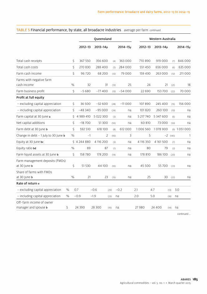
185
Farm performance: broadacre and dairy farms, 2012–13 to 2014–15
ABARESAgricultural commodities – vol. 5 no. 1 • March quarter 2015
TABLE 5 Financial performance, by state, all broadacre industries average per farm
Queensland Western Australia
2012–13 2013–14p 2014–15y 2012–13 2013–14p 2014–15y
Total cash receipts $ 367 550 356 600 (4) 363 000 710 890 919 000 (7) 846 000
Total cash costs $ 270 830 288 400 (5) 284 000 551 450 656 000 (6) 635 000
Farm cash income $ 96 720 68 200 (12) 79 000 159 430 263 000 (12) 211 000
Farms with negative farm
cash income % 32 31 (12) 25 24 21 (21) 18
Farm business profit $ –5 680 –77 400 (13) –54 000 22 690 153 700 (22) 70 000
Profit at full equity
– excluding capital appreciation $ 36 500 –32 600 (28) –11 000 107 890 245 400 (15) 156 000
– including capital appreciation $ –48 340 –95 000 (24) na 101 820 260 100 (19) na
Farm capital at 30 June a $ 4 989 410 5 022 300 (3) na 5 217 740 5 347 600 (6) na
Net capital additions $ –18 700 51 300 (55) na 60 810 73 000 (53) na
Farm debt at 30 June b $ 592 510 618 100 (8) 612 000 1 006 560 1 078 900 (9) 1 051 000
Change in debt – 1 July to 30 June b % –1 2 (93) 3 5 –2 (145) 1
Equity at 30 June bc $ 4 244 880 4 116 200 (3) na 4 116 350 4 161 500 (7) na
Equity ratio bd % 89 87 (1) na 80 79 (2) na
Farm liquid assets at 30 June b $ 158 780 178 200 (14) na 178 810 186 100 (20) na
Farm management deposits (FMDs)
at 30 June b $ 51 530 44 100 (16) na 45 500 55 700 (23) na
Share of farms with FMDs
at 30 June b % 21 23 (15) na 25 30 (22) na
Rate of return e
– excluding capital appreciation % 0.7 –0.6 (29) –0.2 2.1 4.7 (13) 3.0
– including capital appreciation % –0.9 –1.9 (23) na 2.0 5.0 (18) na
Off–farm income of owner
manager and spouse b $ 24 390 28 300 (10) na 27 980 24 400 (14) na
continued
continued ...

186
Farm performance: broadacre and dairy farms, 2012–13 to 2014–15
ABARESAgricultural commodities – vol. 5 no. 1 • March quarter 2015
TABLE 5 Financial performance, by state, all broadacre industries average per farm
South Australia Tasmania
2012–13 2013–14p 2014–15y 2012–13 2013–14p 2014–15y
Total cash receipts $ 479 870 512 900 (8) 508 000 299 490 321 300 (7) 334 000
Total cash costs $ 312 910 344 500 (8) 345 000 229 720 249 900 (8) 230 000
Farm cash income $ 166 960 168 400 (11) 163 000 69 770 71 400 (17) 104 000
Farms with negative farm
cash income % 12 15 (28) 17 11 20 (39) 6
Farm business profit $ 54 440 33 400 (47) 33 000 670 10 400 (100) 31 000
Profit at full equity
– excluding capital appreciation $ 96 800 76 700 (23) 76 000 29 040 40 500 (27) 57 000
– including capital appreciation $ 102 400 79 400 (24) na 56 040 54 300 (26) na
Farm capital at 30 June a $ 3 873 800 4 107 400 (6) na 3 889 340 3 762 500 (8) na
Net capital additions $ 102 890 69 800 (42) na 11 970 48 700 (35) na
Farm debt at 30 June b $ 464 870 470 900 (14) 484 000 363 950 425 500 (13) 386 000
Change in debt – 1 July to 30 June b % 10 2 (198) 1 7 –1 (620) 2
Equity at 30 June bc $ 3 264 250 3 507 100 (6) na 3 559 220 3 290 000 (8) na
Equity ratio bd % 88 88 (1) na 91 89 (1) na
Farm liquid assets at 30 June b $ 203 520 260 200 (22) na 170 530 163 800 (19) na
Farm management deposits
(FMDs) at 30 June b $ 61 650 89 600 (23) na 55 380 61 700 (34) na
Share of farms with FMDs
at 30 June b % 31 37 (13) na 36 34 (27) na
Rate of return e
– excluding capital appreciation % 2.6 1.9 (19) 1.8 0.8 1.1 (26) 1.6
– including capital appreciation % 2.7 2.0 (21) na 1.5 1.5 (27) na
Off–farm income of owner manager
and spouse b $ 27 130 26 300 (10) na 42 160 32 700 (15) na
continued ...
continued

187
Farm performance: broadacre and dairy farms, 2012–13 to 2014–15
ABARESAgricultural commodities – vol. 5 no. 1 • March quarter 2015
TABLE 5 Financial performance, by state, all broadacre industries average per farm
Northern Territory Australia
2012–13 2013–14p 2014–15y 2012–13 2013–14p 2014–15y
Total cash receipts $ 1 754 990 1 580 900 (11) 2 067 000 410 020 447 800 (3) 431 000
Total cash costs $ 1 390 010 1 198 800 (11) 1 387 000 299 750 323 200 (2) 317 000
Farm cash income $ 364 980 382 100 (24) 680 000 110 270 124 600 (4) 114 000
Farms with negative farm
cash income % 63 54 (20) 17 24 23 (8) 22
Farm business profit $ 524 360 429 200 (18) 422 000 13 990 15 100 (38) 3 000
Profit at full equity
– excluding capital appreciation $ 598 120 500 200 (15) 492 000 54 770 57 200 (11) 44 000
– including capital appreciation $ –372 780 476 700 (16) na 44 470 60 400 (15) na
Farm capital at 30 June a $ 16 358 900 17 825 700 (8) na 3 928 910 4 000 100 (2) na
Net capital additions $ 63 020 84 300 (20) na 29 160 40 100 (30) na
Farm debt at 30 June b $ 1 074 970 1 070 200 (24) 980 000 475 860 512 500 (4) 509 000
Change in debt – 1 July to 30 June b % 9 6 (64) –9 3 0 (354) 2
Equity at 30 June bc $ 5 519 380 5 960 400 (9) na 3 312 900 3 346 400 (2) na
Equity ratio bd % 84 85 (4) na 87 87 (1) na
Farm liquid assets at 30 June b $ 56 040 52 600 (52) na 159 730 169 200 (7) na
Farm management deposits
(FMDs) at 30 June b $ 1 820 1 600 () na 41 740 48 300 (8) na
Share of farms with FMDs
at 30 June b % 1 1 () na 23 25 (7) na
Rate of return e
– excluding capital appreciation % 3.5 2.9 (14) 2.8 1.4 1.4 (10) 1.1
– including capital appreciation % –2.2 2.7 (15) na 1.1 1.5 (15) na
Off–farm income of owner manager
and spouse b $ 56 310 74 700 (43) na 32 370 31 500 (6) na
a Excludes leased plant and equipment. b Average per responding farm. c Farm capital minus farm debt. d Equity expressed as a percentage of farm capital. e Rate of return to farm capital at 1 July. p Preliminary estimates. y Provisional estimates. na Not available. Note: Figures in parentheses are standard errors expressed as a percentage of the estimate provided.
continued
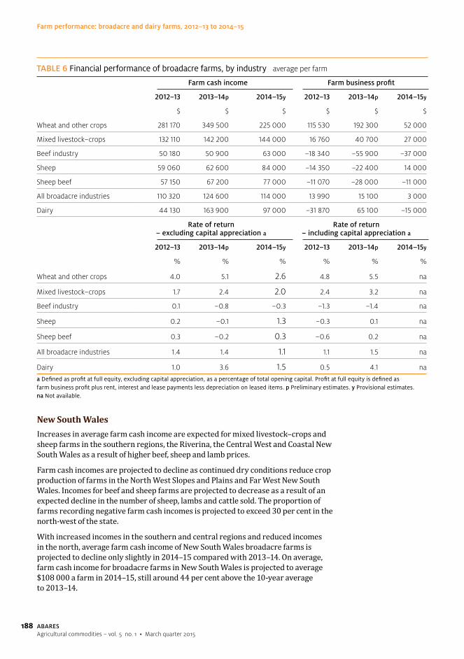
188
Farm performance: broadacre and dairy farms, 2012–13 to 2014–15
ABARESAgricultural commodities – vol. 5 no. 1 • March quarter 2015
New South WalesIncreases in average farm cash income are expected for mixed livestock–crops and sheep farms in the southern regions, the Riverina, the Central West and Coastal New South Wales as a result of higher beef, sheep and lamb prices.
Farm cash incomes are projected to decline as continued dry conditions reduce crop production of farms in the North West Slopes and Plains and Far West New South Wales. Incomes for beef and sheep farms are projected to decrease as a result of an expected decline in the number of sheep, lambs and cattle sold. The proportion of farms recording negative farm cash incomes is projected to exceed 30 per cent in the north-west of the state.
With increased incomes in the southern and central regions and reduced incomes in the north, average farm cash income of New South Wales broadacre farms is projected to decline only slightly in 2014–15 compared with 2013–14. On average, farm cash income for broadacre farms in New South Wales is projected to average $108 000 a farm in 2014–15, still around 44 per cent above the 10-year average to 2013–14.
TABLE 6 Financial performance of broadacre farms, by industry average per farm
Farm cash income Farm business profit
2012–13 2013–14p 2014–15y 2012–13 2013–14p 2014–15y
$ $ $ $ $ $
Wheat and other crops 281 170 349 500 225 000 115 530 192 300 52 000
Mixed livestock–crops 132 110 142 200 144 000 16 760 40 700 27 000
Beef industry 50 180 50 900 63 000 –18 340 –55 900 –37 000
Sheep 59 060 62 600 84 000 –14 350 –22 400 14 000
Sheep beef 57 150 67 200 77 000 –11 070 –28 000 –11 000
All broadacre industries 110 320 124 600 114 000 13 990 15 100 3 000
Dairy 44 130 163 900 97 000 –31 870 65 100 –15 000
Rate of return – excluding capital appreciation a
Rate of return – including capital appreciation a
2012–13 2013–14p 2014–15y 2012–13 2013–14p 2014–15y
% % % % % %
Wheat and other crops 4.0 5.1 2.6 4.8 5.5 na
Mixed livestock–crops 1.7 2.4 2.0 2.4 3.2 na
Beef industry 0.1 –0.8 –0.3 –1.3 –1.4 na
Sheep 0.2 –0.1 1.3 –0.3 0.1 na
Sheep beef 0.3 –0.2 0.3 –0.6 0.2 na
All broadacre industries 1.4 1.4 1.1 1.1 1.5 na
Dairy 1.0 3.6 1.5 0.5 4.1 na
a Defined as profit at full equity, excluding capital appreciation, as a percentage of total opening capital. Profit at full equity is defined as farm business profit plus rent, interest and lease payments less depreciation on leased items. p Preliminary estimates. y Provisional estimates. na Not available.

189
Farm performance: broadacre and dairy farms, 2012–13 to 2014–15
ABARESAgricultural commodities – vol. 5 no. 1 • March quarter 2015
FIGURE 6 Farm cash income, all broadacre farms, New South Wales and Queensland average per farm
2014–15$’000
New South WalesQueensland
y ABARES provisional estimate.
50
100
150
200
2014–15y
2011–12
2008–09
2005–06
2002–03
1999–2000
1996–97
VictoriaVictorian cropping receipts are projected to decline in 2014–15 as a result of reduced winter grain, oilseeds and pulse production resulting from lower yields. Increased receipts from beef, sheep and lambs mainly because of higher prices, are projected to only partially offset reduced crop receipts. Average farm cash income of broadacre farms is projected to be similar to that recorded in 2013–14 in Southern and Eastern Victoria, with reductions in crop receipts offset by increased beef receipts. However, reduced winter crop production is projected to sharply reduce average farm cash income in the Wimmera and Mallee regions. Farm cash income in the Central North is projected to increase slightly as a result of small increases in sheep, lamb, beef and crop receipts.
On average, farm cash income of broadacre farms in Victoria is projected to decline to $68 000 a farm in 2014–15, around 13 per cent below the 10-year average to 2013–14.
QueenslandAverage farm cash incomes are projected to increase in all regions of Queensland in 2014–15 except the Central North and the West and South West. Relatively low farm cash incomes were recorded in most regions in 2013–14 and high turn-off of beef cattle resulted in reduced herd sizes.
Receipts from beef cattle are projected to increase in 2014–15 as a result of higher beef cattle prices and continued high cattle turn-off during the first half of 2014–15. Overall, crop receipts are expected to be reduced, with low receipts from winter grain crops. A large increase is expected in grain sorghum production, but businesses are likely to sell a part of this production in 2015–16.
Average total cash costs are projected to decrease by around 5 per cent in 2014–15, mainly as a result of a projected decrease in expenditure on fodder, fuel and interest payments and a decline in beef cattle purchase expenditure in some regions.
Farm cash income of broadacre farms in Queensland is projected to increase to average $79 000 a farm. This is still around 10 per cent below the 10-year average to 2013–14.

190
Farm performance: broadacre and dairy farms, 2012–13 to 2014–15
ABARESAgricultural commodities – vol. 5 no. 1 • March quarter 2015
FIGURE 7 Farm cash income, all broadacre farms, South Australia and Western Australia average per farm
2014–15$’000
Western AustraliaSouth Australia
y ABARES provisional estimate.
50
100
150
200
250
300
2014–15y
2011–12
2008–09
2005–06
2002–03
1999–2000
1996–97
South AustraliaSouth Australian broadacre farm cash incomes are projected to decrease slightly, to average $163 000 a farm in 2014–15. This would still be around 32 per cent above the 10-year average to 2013–14.
Reduced winter crop production resulting from lower yields, together with lower wheat prices, is projected to result in average farm cash income decreasing in all South Australian regions except the Northern Pastoral region. Reduced expenditure on fuel, interest and fodder in the Northern Pastoral region is projected to result in a slight increase in projected farm cash income for farms in the region.
Crop receipts in 2014–15 are projected to decline by around 8 per cent, with pool payments for grain delivered in 2013–14 partly cushioning a decline in 2014–15 grain receipts. Wool receipts are also expected to be lower. Average total cash costs are projected to remain relatively unchanged, with reduced expenditure on fuel, interest payments and crop handling and marketing offsetting increases in other categories of expenditure.
Western AustraliaA decline in winter grain production after the record crop production in Western Australia in 2013–14 and lower wheat prices are projected to result in a decrease in average farm cash income in Western Australia, particularly in the Central and South Wheat Belt. The impact of the reduction in crop production on receipts is expected to be partly offset by pool payments received in 2014–15 for grain delivered in 2013–14 and by increased receipts from sheep and lambs resulting from higher prices.
In the northern pastoral regions of the Kimberley and Pilbara, increased sales of beef cattle for live export and higher beef cattle prices are projected to increase farm receipts and raise average farm cash income.
Overall, Western Australian broadacre farm cash incomes are projected to decrease to average $211 000 a farm in 2014–15. If achieved, this would still be around 30 per cent above the 10-year average to 2014–15.

191
Farm performance: broadacre and dairy farms, 2012–13 to 2014–15
ABARESAgricultural commodities – vol. 5 no. 1 • March quarter 2015
TasmaniaTasmanian broadacre farm cash incomes are projected to increase to average $104 000 a farm in 2014–15, as a result of higher beef cattle, lamb, wool and crop receipts. Receipts from crops are projected to increase by around 5 per cent, with the largest increase in receipts from oilseed poppies, vegetables and a range of other horticultural and vegetable crops. While receipts are expected to increase, average total cash costs are expected to decline resulting from reduced expenditure on fuel, interest payments and livestock purchases and despite increased expenditure on contracts and hired labour.
Northern TerritoryMany farm businesses in the upper Northern Territory derive a large share of their total cash receipts from selling cattle for live export, particularly to Indonesia. Numbers of cattle sold for live export declined between 2009–10 and 2012–13, before rebounding strongly in 2013–14. They are expected to remain high in 2014–15. As a result of the expansion of the live export trade in 2013–14 and 2014–15, cattle for this market are now also being sourced from a much expanded area of northern Australia.
In 2013–14 farm cash income increased to average $382 100 a farm. While turn-off of cattle increased slightly, average prices received were lower than in 2012–13. Total cash receipts declined slightly as a result, but total farm cash costs declined by much more—mainly as a result of reduced purchases of cattle and transfer of cattle on to Northern Territory properties by farm businesses with properties interstate.
In 2014–15 total farm cash receipts are expected to rise by around 30 per cent, resulting from an estimated increase in turn-off of cattle and higher average prices received per head sold. Average total cash costs are projected to increase by around 20 per cent, partly offsetting higher farm receipts—with higher expenditure on fodder, hired labour and beef cattle purchases. With increased cattle turn-off, expenditure on freight and marketing is also expected to rise. The high turn-off is projected to result in a reduction in herd size.
Farm cash income is projected to increase in all Northern Territory regions in 2014–15, with the largest increases in the Victoria River District–Katherine and the Top End.
Overall, Northern Territory farm cash incomes are projected to increase to average $680 000 a farm in 2014–15, well above the 10-year average to 2013–14 of $312 000 a farm.

192
Farm performance: broadacre and dairy farms, 2012–13 to 2014–15
ABARESAgricultural commodities – vol. 5 no. 1 • March quarter 2015
Performance, by industryFarm financial performance in 2013–14 and projected performance in 2014–15, and how it ranks in historical terms, also varies markedly across industries.
TABLE 7 Financial performance, by industry, broadacre and dairy industries average per farm
Wheat and other crops industry Mixed livestock–crops industry
2012–13 2013–14p 2014–15y 2012–13 2013–14p 2014–15y
Total cash receipts $ 945 360 1 085 000 (4) 934 000 479 800 510 900 (5) 504 000
Total cash costs $ 664 190 735 600 (4) 709 000 347 690 368 700 (6) 360 000
Farm cash income $ 281 170 349 500 (7) 225 000 132 110 142 200 (9) 144 000
Farms with negative farm cash income % 19 9 (21) 27 16 20 (17) 16
Farm business profit $ 115 530 192 300 (12) 52 000 16 760 40 700 (36) 27 000
Profit at full equity
– excluding capital appreciation $ 208 420 291 100 (8) 149 000 67 970 91 700 (17) 75 000
– including capital appreciation $ 253 260 310 800 (9) na 95 900 121 400 (19) na
Farm capital at 30 June a $ 5 375 470 5 828 000 (4) na 3 964 150 3 895 900 (4) na
Net capital additions $ 111 370 139 000 (28) na 10 360 52 700 (47) na
Farm debt at 30 June b $ 1 117 200 1 173 600 (7) 1 152 000 546 960 570 900 (10) 562 000
Change in debt – 1 July to 30 June b % 4 0 (451) 2 3 0 (807) 2
Equity at 30 June bc $ 4 229 920 4 632 800 (5) na 3 346 660 3 291 000 (4) na
Equity ratio bd % 79 80 (1) na 86 85 (1) na
Farm liquid assets at 30 June b $ 203 320 309 700 (16) na 143 220 133 100 (9) na
Farm management deposits (FMDs)
at 30 June b $ 80 530 120 500 (13) na 48 030 51 800 (12) na
Share of farms with FMDs at 30 June b % 29 40 (10) na 32 33 (11) na
Rate of return e
– excluding capital appreciation % 4.0 5.1 (8) 2.6 1.7 2.4 (16) 2.0
– including capital appreciation % 4.8 5.5 (9) na 2.4 3.2 (18) na
Off-farm income of owner–manager
and spouse b $ 29 650 29 600 (12) na 28 920 27 300 (13) na
continued ...
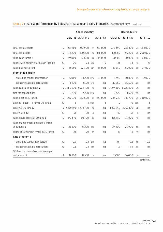
193
Farm performance: broadacre and dairy farms, 2012–13 to 2014–15
ABARESAgricultural commodities – vol. 5 no. 1 • March quarter 2015
TABLE 7 Financial performance, by industry, broadacre and dairy industries average per farm
Sheep industry Beef industry
2012–13 2013–14p 2014–15y 2012–13 2013–14p 2014–15y
Total cash receipts $ 231 260 242 900 (7) 263 000 230 490 246 100 (5) 263 000
Total cash costs $ 172 200 180 300 (6) 178 000 180 310 195 200 (6) 200 000
Farm cash income $ 59 060 62 600 (15) 84 000 50 180 50 900 (11) 63 000
Farms with negative farm cash income % 26 24 (23) 16 34 34 (11) 27
Farm business profit $ –14 350 –22 400 (37) 14 000 –18 340 –55 900 (10) –37 000
Profit at full equity
– excluding capital appreciation $ 6 060 –3 200 (270) 33 000 4 910 –30 800 (18) –12 000
– including capital appreciation $ –8 190 3 500 (611) na –49 360 –56 600 (23) na
Farm capital at 30 June a $ 2 680 670 2 604 100 (4) na 3 897 400 3 928 400 (3) na
Net capital additions $ –2 790 –12 200 (224) na 9 520 13 600 (152) na
Farm debt at 30 June b $ 232 970 252 600 (12) 247 000 284 230 332 700 (8) 340 000
Change in debt – 1 July to 30 June b % 8 2 (202) 2 2 0 (881) 4
Equity at 30 June bc $ 2 399 150 2 294 700 (5) na 3 352 850 3 292 100 (4) na
Equity ratio bd % 91 90 (1) na 92 91 (1) na
Farm liquid assets at 30 June b $ 179 610 103 700 (15) na 156 810 174 900 (13) na
Farm management deposits (FMDs)
at 30 June b $ 33 890 31 200 (25) na 27 400 25 900 (16) na
Share of farms with FMDs at 30 June b % 23 20 (17) na 17 16 (17) na
Rate of return e
– excluding capital appreciation % 0.2 –0.1 (271) 1.3 0.1 –0.8 (18) –0.3
– including capital appreciation % –0.3 0.1 (612) na –1.3 –1.4 (23) na
Off-farm income of owner–manager
and spouse b $ 32 390 31 300 (11) na 35 180 36 400 (11) na
continued ...
continued

194
Farm performance: broadacre and dairy farms, 2012–13 to 2014–15
ABARESAgricultural commodities – vol. 5 no. 1 • March quarter 2015
TABLE 7 Financial performance, by industry, broadacre and dairy industries average per farm
Sheep–beef industry Dairy industry
2012–13 2013–14p 2014–15y 2012–13 2013–14p 2014–15y
Total cash receipts $ 236 010 269 600 (10) 261 000 573 840 740 000 (6) 677 000
Total cash costs $ 178 860 202 400 (9) 184 000 529 710 576 100 (6) 579 000
Farm cash income $ 57 150 67 200 (19) 77 000 44 130 163 900 (9) 97 000
Farms with negative farm cash income % 16 13 (24) 15 33 16 (45) 17
Farm business profit $ –11 070 –28 000 (41) –11 000 –31 870 65 100 (22) –15 000
Profit at full equity
– excluding capital appreciation $ 9 320 –5 500 (230) 9 000 34 550 135 500 (12) 55 000
– including capital appreciation $ –18 220 6 200 (396) na 19 010 152 900 (22) na
Farm capital at 30 June a $ 3 304 720 3 498 300 (7) na 3 693 040 3 819 100 (7) na
Net capital additions $ 42 250 18 300 (108) na 115 690 68 200 (43) na
Farm debt at 30 June b $ 263 400 295 800 (19) 273 000 765 970 821 400 (8) 854 000
Change in debt – 1 July to 30 June b % 6 1 (647) 0 4 0 (930) 2
Equity at 30 June bc $ 2 915 670 3 060 600 (10) na 2 910 970 2 968 700 (7) na
Equity ratio bd % 92 91 (1) na 79 78 (2) na
Farm liquid assets at 30 June b $ 104 890 104 400 (26) na 186 650 190 300 (17) na
Farm management deposits (FMDs)
at 30 June b $ 22 270 25 600 (45) na 26 580 25 900 (34) na
Share of farms with FMDs at 30 June b % 16 21 (29) na 17 19 (32) na
Rate of return e
– excluding capital appreciation % 0.3 –0.2 (233) 0.3 1.0 3.6 (10) 1.5
– including capital appreciation % –0.6 0.2 (396) na 0.5 4.1 (21) na
Off-farm income of owner–manager
and spouse b $ 34 670 26 800 (18) na 20 270 23 000 (12) na
a Excludes leased plant and equipment. b Average per responding farm. c Farm capital minus farm debt. d Equity expressed as a percentage of farm capital. e Rate of return to farm capital at 1 July. p Preliminary estimates. y Provisional estimates. na Not available. Note: Figures in parentheses are standard errors expressed as a percentage of the estimate provided.
continued

195
Farm performance: broadacre and dairy farms, 2012–13 to 2014–15
ABARESAgricultural commodities – vol. 5 no. 1 • March quarter 2015
Wheat and other crops industryAverage farm cash income for the wheat and other crops industry increased in 2013–14 to average $349 500 a farm, with higher prices for wheat, grain sorghum and pulses and increased grain production, particularly in South Australia and Western Australia.
In 2014–15 farm cash income for the wheat and other crops industry is projected to decline to average $225 000 a farm. This is mainly a result of lower production in all the major producing states, reflecting a decline from the high yields in 2013–14 combined with reduced prices for wheat, pulses and oilseeds. If realised, projected 2014–15 farm cash income will still be around 14 per cent higher than the 10-year average to 2013–14.
In 2014–15 crop receipts are projected to decline by 14 per cent and total cash costs are projected to decrease by around 4 per cent, mainly as a result of the lower cost of harvesting and marketing a smaller crop together with reduced fuel and interest payment expenditure. Expenditure is projected to decrease in most cost categories, with the exception of crop and pasture chemicals.
Wheat and other crops industry farms are projected to record the highest average rate of return excluding capital appreciation (2.6 per cent) of industries surveyed in 2014–15. However, rates vary across the states and territories. Wheat and other crops industry farms surveyed recorded the highest average rate of return among broadacre industries in 19 of the past 20 years.
FIGURE 8 Farm cash income, grains industries average per farm
2014–15$’000
Wheat and other cropsMixed livestock crops
y ABARES provisional estimate.
50
100
150
200
250
300
350
400
2014–15y
2011–12
2008–09
2005–06
2002–03
1999–2000
1996–97

196
Farm performance: broadacre and dairy farms, 2012–13 to 2014–15
ABARESAgricultural commodities – vol. 5 no. 1 • March quarter 2015
FIGURE 9 Farm cash income, sheep industries average per farm
2014–15$’000
Sheep–beefSheep
y ABARES provisional estimate.
30
60
90
120
150
2014–15y
2011–12
2008–09
2005–06
2002–03
1999–2000
1996–97
FIGURE 10 Farm cash income, beef industry average per farm
y ABARES provisional estimate.
20
40
60
80
100
120
2014–15$’000
2014–15y
2011–12
2008–09
2005–06
2002–03
1999–2000
1996–97
Mixed livestock–crops industryAverage farm cash income for the mixed livestock–crops industry increased in 2013–14 to average $142 200, with increases in sheep, wool and grain receipts. Only a small increase occurred in total cash costs, with reductions in expenditure on interest payments and fuel.
In 2014–15 crop receipts are projected to decrease by around 5 per cent for farms in this industry. Small increases in sheep and lamb receipts are not expected to offset the effects of reduced crop receipts resulting from reduced production and prices for wheat, oilseeds and pulses.
197
Farm performance: broadacre and dairy farms, 2012–13 to 2014–15
ABARESAgricultural commodities – vol. 5 no. 1 • March quarter 2015
Total cash costs are projected to decrease by around 2 per cent, mainly because of projected decreases in expenditure on fodder, fuel, livestock purchases and interest payments. In addition, crop handling and marketing costs will be lower because of the harvest of a smaller crop.
Average farm cash income for mixed livestock–crops industry farms is projected to increase slightly to an average of $144 000 a farm in 2014–15, around 50 per cent above the 10-year average to 2013–14.
Sheep industryIn 2013–14 higher prices for adult sheep and lambs resulted in an increase in average farm cash income for sheep industry farms to $62 600 a farm, despite a small reduction in receipts from wool.
In 2014–15 farm cash income for sheep industry farms is projected to increase to average $84 000 a farm, mainly as a result of higher sheep and lamb prices. If achieved, farm cash income for sheep industry farms would be around 41 per cent above the 10-year average to 2013–14 of $60 000 a farm (in real terms).
Sheep–beef industryIn 2013–14 receipts from the sale of sheep, lambs and wool increased, resulting from higher prices for adult sheep and lambs together with higher turn-off of sheep. In addition, receipts from the sale of beef cattle increased as turn-off increased with drier seasonal conditions in Queensland, northern New South Wales, Victoria and South Australia. Farm cash income for sheep–beef industry farms increased to average $67 200 a farm.
In 2014–15 farm cash income for sheep–beef industry farms is projected to increase to average $77 000 a farm as a result of higher beef cattle and sheep prices and a small reduction in total cash costs. If achieved, this would be around 2 per cent below the 10-year average to 2013–14.
Beef industryIn 2013–14 dry seasonal conditions led to an increase in net cattle turn-off and a decrease in herd sizes in both northern and southern Australia. Increased turn-off more than offset lower average sale prices for beef cattle and resulted in average beef cattle receipts increasing by 8 per cent for beef industry farms. Increased expenditure on fodder, fuel and interest payments mostly offset the increase in beef cattle receipts. As a result, average farm cash income for beef industry farms remained similar to 2012–13 and averaged $50 900 a farm in 2013–14.
Beef cattle turn-off remained high in the first half of 2014–15. A sharp decline is expected in the second half of 2014–15 as seasonal conditions improve across many regions previously affected by dry seasonal conditions. Relatively high turn-off combined with higher saleyard prices for cattle is projected to result in an increase in farm receipts. This increase is projected to more than offset a small increase in average total cash costs, resulting in average farm cash income of beef industry farms increasing to $63 000 a farm. The farm cash income projected in 2014–15 is still around 2 per cent below the 10-year average to 2013–14.

198
Farm performance: broadacre and dairy farms, 2012–13 to 2014–15
ABARESAgricultural commodities – vol. 5 no. 1 • March quarter 2015
Dairy industryIn 2013–14 average farm cash incomes rebounded strongly, with large increases in milk prices for milk producers in Victoria, Tasmania, South Australia and southern New South Wales and smaller increases for producers in other states and regions. Nationally, average farm cash income increased from $44 130 in 2012–13 to $163 900 in 2013–14.
In 2014–15 average farm cash incomes are projected to decline in most states, with a decline in farmgate milk prices in most states and regions except Queensland, northern New South Wales and Western Australia. Milk production is expected to increase in all states except Queensland and South Australia, with a large increase expected in Tasmania.
Average farm cash income is projected to decline to $86 600 a farm in Victoria, $90 200 in South Australia and $108 700 in New South Wales. The reduction in farm cash income is expected to be much smaller in Tasmania, where a larger increase in milk production is expected. Farm cash income in Tasmania is projected to average $201 900 a farm. Farm cash income is expected to remain largely unchanged in Queensland, at an average of $72 600 a farm. In Western Australia, farm cash income is projected to increase slightly to average $166 400 a farm.
When variations to projected farm cash incomes of dairy farms across Australia are taken into account, the overall average farm cash income of Australian dairy farms is projected to decrease to average $97 000 a farm in 2014–15, around 14 per cent below the 10-year average to 2013–14.
FIGURE 11 Farm cash income, dairy industry average per farm
y ABARES provisional estimate.
30
60
90
120
150
180
2014–15$’000
2014–15y
2011–12
2008–09
2005–06
2002–03
1999–2000
1996–97

199
Farm performance: broadacre and dairy farms, 2012–13 to 2014–15
ABARESAgricultural commodities – vol. 5 no. 1 • March quarter 2015
TAB
LE 8
Fin
anci
al p
erfo
rman
ce, d
airy
indu
stry
, by
stat
e a
vera
ge p
er fa
rm
Farm
cas
h in
com
eFa
rm b
usin
ess
profi
t a
Rat
e of
ret
urn
excl
udin
g ca
pita
l ap
prec
iati
on b
Rat
e of
ret
urn
incl
udin
g ca
pita
l ap
prec
iati
on
2012
–13
2013
–14
p20
14–1
5y20
12–1
320
13–1
4p
2014
–15y
2012
–13
2013
–14
p20
14–1
5y20
12–1
320
13–1
4p
2014
–15y
$$
$$
$$
%%
%%
%%
Dai
ry in
dust
ry
New
Sou
th W
ales
61
380
123
10
0(1
5) 1
09
00
0–2
1 64
0 8
50
0(2
44)
–7 0
00
0.9
1.8(2
9)1.3
0.6
8.6
(69)
na
Vict
oria
32
490
173
70
0(1
3) 8
7 0
00
–35
920
77
600
(25)
–23
00
00.
94.
3(1
3)1.3
0.5
3.9
(22)
na
Que
ensl
and
71
520
73
800
(30)
73
00
0–1
1 54
0–1
6 90
0(1
57)
–38
00
00.
70.
8(9
5)0.
1–1
.20.
4(1
85)
na
Wes
tern
Aus
tral
ia 1
33 3
70 1
61 3
00
(10)
166
00
0 7
5 71
0 7
0 9
00
(31)
31
00
01.8
2.1
(18)
1.50.
22.
2(1
8)na
Sout
h Au
stra
lia 8
1 25
0 1
63 0
00
(24)
90
00
0–4
5 36
0 6
2 90
0(5
7)–3
2 0
00
0.8
3.7
(22)
1.52.
23.
3(3
2)na
Tasm
ania
44
100
238
10
0(1
0) 2
02 0
00
–66
840
123
10
0(1
8) 7
9 0
00
1.44.
7(1
0)3.
90.
94.
4(3
9)na
Aust
ralia
44
130
163
90
0(9
) 9
7 0
00
–31
870
65
100
(22)
–15
00
01.0
3.6
(10)
1.50.
54.
1(2
1)na
a D
efine
d as
farm
cas
h in
com
e pl
us b
uild
-up
in t
radi
ng s
tock
s, le
ss d
epre
ciat
ion
and
the
impu
ted
valu
e of
ope
rato
r pa
rtne
r an
d fa
mily
labo
r. b
Defi
ned
as p
rofit
at f
ull e
quit
y, e
xclu
ding
cap
ital
app
reci
atio
n,
as a
per
cent
age
of t
otal
ope
ning
cap
ital
. Pro
fit a
t ful
l equ
ity
is d
efine
d as
farm
bus
ines
s pr
ofit p
lus
rent
, int
eres
t and
leas
e pa
ymen
ts le
ss d
epre
ciat
ion
on le
ased
item
s. p
Pre
limin
ary
esti
mat
es.
y Pr
ovis
iona
l est
imat
es. n
a N
ot a
vaila
ble.
N
ote:
Fig
ures
in p
aren
thes
es a
re s
tand
ard
erro
rs e
xpre
ssed
as
a pe
rcen
tage
of t
he e
stim
ate
prov
ided
.

200
Farm performance: broadacre and dairy farms, 2012–13 to 2014–15
ABARESAgricultural commodities – vol. 5 no. 1 • March quarter 2015
Farm investmentProducers’ capacity to generate farm income will be influenced by their past investments in additional land to expand the scale of their farming activities and in new infrastructure, plant and machinery to boost productivity in the longer term.
Over the decade to 2013–14 broadacre and dairy farmers invested heavily in land, plant and machinery. In 2013–14 new investment remained relatively high in historical terms.
FIGURE 12 Proportion of farms acquiring land percentage of farms
%
p ABARES preliminary estimate.
2
4
6
8
10
2013–14p
2010–11
2007–08
2004–05
2001–02
1998–99
1995–96
In 2013–14 the proportion of broadacre and dairy farms acquiring additional land through purchase or leasing increased slightly. Around 6 per cent of broadacre farms acquired additional land, close to the average for the previous 10 years but well down on the proportion acquiring land in the late 1990s and early 2000s.
Land values reported for broadacre and dairy farms have declined in some regions since 2009–10, particularly in the pastoral zone of northern Australia. Reported land values declined slightly in the high rainfall and wheat–sheep zones in 2011–12 and 2012–13, before increasing slightly in 2013–14 in southern and western wheat–sheep zone regions. Reported land values in 2013–14 were up to 30 per cent below those reported in 2007–08 in some pastoral regions of northern Australia, particularly where very large increases were recorded over the previous decade. Farmers in the high rainfall zone reported much smaller reductions in land values, of around 7 per cent.
Average land prices for broadacre farms increased sharply relative to the cash receipts per hectare generated by farming activity between 2001–02 and 2007–08 and then declined slightly to 2013–14.
On broadacre farms, the ratio of average land price per hectare to total cash receipts per hectare doubled from an average of 5:1 in the three years to 2001–02 to 10:1 in the three years to 2009–10. The ratio increased from 7:1 to 14:1 in the high rainfall zone and from 4:1 to 8:1 in the wheat–sheep zone. The largest increase was reported in the pastoral zone, where the ratio increased from 4:1 to 9:1.

201
Farm performance: broadacre and dairy farms, 2012–13 to 2014–15
ABARESAgricultural commodities – vol. 5 no. 1 • March quarter 2015
Average receipts per hectare have risen in recent years in the southern and western wheat–sheep zone, reducing the gap between land values and returns per hectare. Similarly, the gap between land values and returns per hectare has reduced in northern pastoral regions with lower land values and increased returns per hectare from beef cattle projected in 2014–15.
FIGURE 13 Land prices for broadacre farms
index100=1977–78
Wheat–sheepPastoral
p ABARES preliminary estimate.
High rainfall
100
200
300
400
500
600
700
800
2013–14p
2009–10
2005–06
2001–02
1997–98
1993–94
1989–90
1985–86
1981–82
1977–78
FIGURE 14 Land prices and receipts per hectare, broadacre farms average per farm
2014–15$/ha
p ABARES preliminary estimate.
100
200
300
400
500
600 Land value per hectareReceipts per hectare
2013–14p
2010–11
2007–08
2004–05
2001–02
1998–99
1995–96

202
Farm performance: broadacre and dairy farms, 2012–13 to 2014–15
ABARESAgricultural commodities – vol. 5 no. 1 • March quarter 2015
While only a relatively small proportion of farms buy land in any one year, most producers make some annual investment in plant, vehicles, machinery and/or infrastructure. However, the value of land purchases typically dominates total investment because of the much larger average value of land transactions.
Net investment in plant, vehicles, machinery and farm infrastructure (non-land net capital additions) for broadacre farms has been relatively high since 2007–08. Net investment is the difference between the total value of plant, vehicles, machinery and farm infrastructure purchased and the total value of those items sold or disposed of. In addition to acquiring new capital items and replacing old items, farms must cover ongoing maintenance and repair of existing plant, vehicles, machinery and farm infrastructure. This expenditure is recorded in ABARES surveys as the cash cost of repairs and maintenance. Most reported annual expenditure on repairs and maintenance is actually the capital cost of replacing and upgrading items of farm capital, such as fencing, stockyards, buildings and watering facilities. Annual expenditure on repairs and maintenance is strongly correlated with farm income. Expenditure on repairs and maintenance rises in years of high farm cash income and falls in years of lower farm cash income.
FIGURE 15 Composition of non-land net capital additions, broadacre farms average per farm
Computer, office, workshop and other equipment
Livestock handling
2014–15$’000
Repairs andmaintenance
p ABARES preliminary estimate.
Buildings, fences, yards and structures
Grain storageAccommodation
VehiclesIrrigation equipment
Harvesting andhandlingCultivation, sowing,fertiliser and spraying
Tractors
10
20
30
40
50
2013–14p
2011–12
2009–10
2007–08
2005–06
In the three years to 2013–14, investment in crop growing plant and machinery on broadacre farms continued at a high level, but investment in equipment related to livestock production or used more generally across all farm activities declined in real terms.
Investment by broadacre farms in tractors, crop harvesting and handling equipment, cultivation, sowing and planting equipment accounted for 62 per cent of net capital additions; vehicles 26 per cent; buildings, accommodation, yards and livestock handling equipment and watering facilities 10 per cent; and computing and workshop equipment 2 per cent.
Investment by dairy farms in crop growing and handling machinery was also high, averaging 64 per cent of net capital additions in 2013–14.

203
Farm performance: broadacre and dairy farms, 2012–13 to 2014–15
ABARESAgricultural commodities – vol. 5 no. 1 • March quarter 2015
Most of the rising trend in real expenditure on net capital additions and repairs and maintenance over the past 20 years for both broadacre and dairy farms resulted from an increase in the average scale of operations of farms, increased production of crops and increased intensification of enterprises.
Farm debtDebt is an important source of funds for farm investment and ongoing working capital for the broadacre and dairy industries, because more than 95 per cent of farms in these sectors are family owned and operated. Funding by family farms for expansion and improvement is limited to the funds available to the family, the profits the business can generate and the funds it can borrow.
Farm business debt more than doubled in real terms in the decade to 2009. Nationally, total indebtedness of the agriculture, forestry and fishing industries to institutional lenders increased from $40.7 billion at 30 June 2001 to $72.0 billion in real terms by 77 per cent at 30 June 2009. Total rural debt subsequently declined in real terms to $64.6 billion at 30 June 2013. Bank lending accounts for 95 per cent of total institutional lending, and bank lending declined from $65.6 billion at 31 December 2009 to $60.7 billion at 30 June 2014 (RBA 2015a, 2015b).
Change in farm debt over time is the balance between the amount of principal repaid and the increase in principal owed (new borrowing). The increase in broadacre and dairy industry debt is the result of increased borrowing together with reduced loan principal repayments through much of the 2000s.
Lower interest rates from the late 1990s and increased lending fuelled the boom in land prices, raising farm equity (net wealth) and inducing lenders to provide more finance. This continued until a correction in land values after 2009 in some regions and tightened lending practices by banks in recent years. In addition, provision of interest subsidies to farmers in drought through exceptional circumstances arrangements supported debt servicing. In many regions this assistance was sustained for most of the 2000s.
FIGURE 16 Composition of farm business debt, broadacre farms average per farm
Other debt
2014–15$’000
Buildings and structures
p ABARES preliminary estimate.
Land developmentMachinery, plant and vehiclesReconstructed debt
Land purchaseWorking capital
100
200
300
400
500
600
2013–14p
2010–11
2007–08
2004–05
2001–02
1998–99
1995–96

204
Farm performance: broadacre and dairy farms, 2012–13 to 2014–15
ABARESAgricultural commodities – vol. 5 no. 1 • March quarter 2015
Borrowing to fund new on-farm investment, particularly purchase of land, machinery and vehicles, made the largest contribution to the increase in average broadacre farm debt. In particular, debt to fund land purchase accounted for the largest share of debt—an estimated 41 per cent of average debt of broadacre farms in 2013–14.
Several factors in addition to lower interest rates contributed to the growth in debt over this period. Structural adjustment resulted in broadacre farmers changing the mix of commodities produced and increasing farm size. An increase in the average size of farm enterprises resulted in higher borrowing for ongoing working capital. Factors that contributed to increased working capital debt included movement away from less input-intensive wool production into more intensive cropping, changes in grain payment methods, higher variability in crop incomes compared with livestock incomes and movement to more intensive production technologies involving greater use of purchased inputs such as herbicides.
In addition, loan repayment slowed and borrowing to meet working capital requirements increased for producers during the 2000s drought. Working capital debt accounted for 39 per cent of average farm debt for broadacre farms in 2012–13.
Similar to broadacre farm debt, average dairy farm debt more than doubled between 2000–01 and 2013–14, mainly resulting from an increase in average farm size. The increase in average debt a farm is modest relative to the increase in the average number of litres of milk produced a farm (a measure of capacity to generate income to service debt). Borrowing has increased most for land purchase and on-farm investment. Borrowing for ongoing working capital has risen with increases in average herd size and with greater mechanisation and intensification of dairy enterprises.
Growth in average debt a farm business in the broadacre and dairy industries has slowed in recent years as a result of a reduction in new borrowing and continued debt repayments. Dairy industry debt increased by around 4 per cent during 2013–14 to average $783 700 a farm, but broadacre debt is estimated to have remained largely unchanged at an average of $512 500 a farm at 30 June 2014.
Change in farm debt 2013–14At the national level, no change was recorded in broadacre and dairy farm debt during 2013–14. Around 40 per cent of broadacre and dairy industry farm businesses reduced overall farm debt in 2013–14, with the largest reductions in regions with high farm cash incomes during 2013–14 including the Central and South Wheat Belt of Western Australia, the Eyre Peninsula in South Australia and southern New South Wales. In contrast, debt increased on 27 per cent of broadacre and dairy farm businesses in 2013–14, particularly for farms undertaking additional investment and farms subject to drought.
Cash flow surplus (profit) was the main source of funds used to reduce farm debt in 2013–14, accounting for 56 per cent of the reduction in principal owed by broadacre and dairy farms. A further 16 per cent was repaid from the sale of farm assets; 10 per cent from liquid assets such as bank deposits and farm management deposits; 6 per cent with off-farm income; 5 per cent from sale of non-farm assets, such as investment property and shares; and 7 per cent from other sources.

205
Farm performance: broadacre and dairy farms, 2012–13 to 2014–15
ABARESAgricultural commodities – vol. 5 no. 1 • March quarter 2015
Land purchase accounted for 37 per cent of the increase in principal owed by broadacre and dairy farms in 2013–14. A further 29 per cent went to purchase of farm machinery and vehicles; 26 per cent to fund shortfalls in cash flow (business losses); 3 per cent for farm development; 2 per cent for livestock purchase; 1 per cent for purchase of non-farm assets; and 3 per cent for other purposes. Most of the ‘other’ category went to funding change in business ownership or partnership arrangements.
FIGURE 17 Reason for change in farm business debt, all broadacre and dairy farms, 2013–14p average per farm
Other
Purchase of non-farm assets
Livestock purchase
Farm development
Cash �ow shortfall
Machinery andvehicle purchase
Land purchase
Other
Sale of non-farm assets
O�-farm income
Reduction in liquid assetsand FMDs a
Sale of farm assets
Cash �ow surplus
$’000
$’000
a Farm management deposits. p ABARES preliminary estimate. Note: Other includes borrowing to fund changes in farm business ownership/partnership.
10 20 30 40
10 20 30 40
Reduction
Increase
Change in debt for farms affected by droughtFarm debt increased for 34 per cent of farms affected by drought (mainly in Queensland and northern New South Wales) in 2013–14. Debt for farm businesses affected by drought increased by an average of 5 per cent, compared with an average reduction of 1 per cent in debt for all other broadacre and dairy farms in 2013–14. This increase is relatively small when compared with increases in farm debt recorded by drought-affected farms during the 2000s, when increases averaged in excess of 10 per cent in several years.

206
Farm performance: broadacre and dairy farms, 2012–13 to 2014–15
ABARESAgricultural commodities – vol. 5 no. 1 • March quarter 2015
Cash flow shortfall (business losses) accounted for 57 per cent of the increase in principal owed by drought-affected broadacre and dairy farms in 2013–14. A further 26 per cent went to the purchase of land; 12 per cent to the purchase of farm machinery and vehicles; 3 per cent to farm development, including provision of watering facilities; and 1 per cent to other purposes.
Debt remained largely unchanged for 36 per cent of farms affected by drought and was reduced for around 30 per cent of farms. The main contributor to reductions in farm debt on drought-affected farms was cash flow, mainly from sale of livestock. This accounted for 45 per cent of the reduction in principal owed. Farm businesses reduced a further 20 per cent using liquid assets, including bank deposits and farm management deposits; 12 per cent from the sale of farm assets; 1 per cent from sale of non-farm assets; and 3 per cent from other sources.
FIGURE 18 Reason for change in farm business debt, broadacre and dairy farms affected by drought, 2013–14pp average per farm
Other
Purchase of non-farm assets
Livestock purchase
Farm development
Cash �ow shortfall
Machinery andvehicle purchase
Land purchase
Other
Sale of non-farm assets
O�-farm income
Reduction in liquid assetsand FMDs a
Sale of farm assets
Cash �ow surplus
$’000
$’000
a Farm management deposits. p ABARES preliminary estimate. Note: Other includes borrowing to fund changes in farm business ownership/partnership.
10 20 30 40
10 20 30 40
Reduction
Increase

207
Farm performance: broadacre and dairy farms, 2012–13 to 2014–15
ABARESAgricultural commodities – vol. 5 no. 1 • March quarter 2015
Drought affects farm businesses in many ways in addition to debt. Livestock numbers, stocks of grain and fodder and, typically, liquid assets available are reduced to fund cash outlays. The combined effect in 2013–14 was that farm business equity declined for 55 per cent of broadacre and dairy farms affected by drought. On average farm business equity declined by 3 per cent ($90 000), and the average farm equity ratio declined by 1 per cent for farms affected by drought.
For large farm businesses (Box 4) affected by drought, farm business debt increased by an average of 4 per cent and farm business equity declined by an average of 5 per cent ($750 000) in 2013–14. The average farm equity ratio declined from 79 per cent to 77 per cent. Large farm businesses generally operate with lower equity ratios, and as a result, incur greater equity reductions in downturns such as drought than smaller farms.
Farm equityThe decline in land values since 2007–08 has reduced farm equity in some regions and prompted financial institutions to tighten lending, restricting access of some farm businesses to further finance.
FIGURE 19 Change in farm business debt and equity, broadacre farms Australia average per farm
Index1999–2000
= 100
%
Farm businessequity
Farm businessdebt
p ABARES preliminary estimate.
Equity ratio (right axis)
100
200
300
400
500
20
40
60
80
100
2013–14p
2010–11
2007–08
2004–05
2001–02
Nevertheless, on average, farm business equity remains strong for broadacre farms, declining only slightly after the large increase that occurred through the 2000s. The average equity ratio for broadacre farms at 30 June 2014 was an estimated 87 per cent, unchanged from 30 June 2013. Around 81 per cent of farms had equity ratios exceeding 80 per cent at 30 June 2014. In some regions farm equity is estimated to have fallen significantly over the three years to June 2014, mainly as a consequence of reported reductions in land values.
One prominent example is the pastoral regions of northern Australia, where land prices are lower resulting from increased caution from land buyers, tighter lending practices by lending institutions and reduced farm profitability as a result of dry seasonal conditions and a decline in beef cattle prices to 2013–14 (ABARES 2014). However, in other regions, farm equity has strengthened because of reduced farm debt and increased capital investment.

208
Farm performance: broadacre and dairy farms, 2012–13 to 2014–15
ABARESAgricultural commodities – vol. 5 no. 1 • March quarter 2015
At the national level, the average equity ratio for dairy farms has declined since 2004–05 as debt levels have increased with increased herd size and milk production. This has been particularly so in regions with increased focus on production of dairy products for export such as Tasmania, Western Victoria and South Australia. The average farm equity ratio of dairy industry farms at 30 June 2014 was 78 per cent, down 1 per cent from 30 June 2013 and around 10 per cent lower than in 2004–05.
Change in farm equity ratios over time should be considered against the background of the increase in average farm size. Equity ratios are typically lower for larger farms because they are generally able to service larger debts.
Distribution of farms by debt and equityThe proportion of broadacre farms with relatively high debt varies across jurisdictions and industries.
Around 36 per cent of broadacre farms in Western Australia and around 23 per cent of Northern Territory farms carried in excess of $1 million in debt at 30 June 2014. The high proportion of farms with debt exceeding $1 million reflects a high proportion of larger businesses in those jurisdictions.
Similarly, around 34 per cent of wheat and other crops industry farms and 26 per cent of dairy industry farms nationally carried in excess of $1 million in debt at 30 June 2014. Both industries have an increasing proportion of large farms.
In contrast, 66 per cent of beef farms and 58 per cent of sheep–beef farms nationally were recorded as having debt less than $100 000 at 30 June 2014. Many of these businesses are small. The number of dairy farms with debt less than $100 000 declined from 21 per cent at 30 June 2012 to 16 per cent at 30 June 2014.
Much of the aggregate broadacre and dairy sector debt is held by a relatively small proportion of mostly larger farms. Around 70 per cent of aggregate broadacre sector debt, at 30 June 2014, was held by just 12 per cent of farms. On average, these were much larger farm businesses, which in aggregate produced around 46 per cent of the total value of broadacre farm production in 2013–14. Similarly, around 45 per cent of aggregate dairy sector debt at 30 June 2014 was held by 9 per cent of farms.

209
Farm performance: broadacre and dairy farms, 2012–13 to 2014–15
ABARESAgricultural commodities – vol. 5 no. 1 • March quarter 2015
TABLE 9 Distribution of broadacre farms, by farm business debt and equity ratio at 30 June 2014 pa percentage of farms
New South Wales Victoria Queensland
Western Australia
South Australia Tasmania
Northern Territory Australia
Farm business debt b
<$100 000 % 51 (8) 61 (6) 51 (7) 35 (17) 53 (13) 60 (11) 50 (33) 52 (4)
$100 000 and
<$250 000 % 16 (19) 13 (24) 9 (23) 7 (41) 8 (48) 11 (49) 1 (134) 12 (12)
$250 000 and
<$500 000 % 13 (17) 11 (20) 11 (21) 7 (42) 10 (26) 11 (42) 7 (126) 11 (10)
$500 000 and <$1m % 8 (17) 8 (22) 13 (17) 15 (27) 17 (23) 3 (53) 19 (69) 11 (9)
$1m and <$2m % 8 (15) 5 (19) 8 (20) 21 (18) 7 (33) 9 (31) 6 (82) 9 (9)
≥$2m % 5 (16) 2 (19) 8 (12) 15 (13) 5 (24) 6 (25) 17 (24) 6 (7)
Total % 100 100 100 100 100 100 100 100
Average farm debt
at 30 June $’000 445 (8) 263 (9) 618 (8) 1 079 (9) 471 (14) 426 (13) 1 070 (24) 512 (4)
Farm business equity ratio bc
≥90 per cent % 65 (5) 75 (4) 67 (5) 46 (12) 62 (10) 81 (4) 61 (24) 65 (3)
80 and <90 per cent % 18 (16) 11 (20) 15 (17) 16 (24) 15 (29) 6 (38) 25 (54) 15 (9)
70 and <80 per cent % 9 (20) 9 (24) 8 (24) 15 (25) 13 (27) 10 (31) 7 (62) 10 (10)
60 and <70 per cent % 4 (22) 3 (37) 6 (24) 11 (23) 7 (30) 2 (35) 1 (130) 5 (11)
<60 per cent % 4 (24) 2 (38) 5 (23) 12 (21) 4 (46) 1 (44) 6 (61) 5 (12)
Total % 100 100 100 100 100 100 100 100
Average farm
business equity
ratio at 30 June % 88 (1) 91 (1) 86 (1) 80 (2) 89 (2) 89 (1) 85 (4) 87 (1)
Population of farms no. 18 000 12 400 9 700 6 400 6 500 900 200 54 000a Excludes debt for large corporate farms. b Average per responding farm. c Equity ratio defined as total owned business capital at 30 June less debt as a percentage of total owned business capital. p ABARES preliminary estimates. Note: Figures in parentheses are standard errors expressed as a percentage of the estimate provided.

210
Farm performance: broadacre and dairy farms, 2012–13 to 2014–15
ABARESAgricultural commodities – vol. 5 no. 1 • March quarter 2015
Debt servicingFor the broadacre and dairy industries, the proportion of farm receipts needed to fund interest payments rose substantially between 2001–02 and 2007–08. This resulted from a large increase in farm debt and reduced farm receipts after extended drought conditions. Interest rate subsidies paid to farm businesses as drought assistance partially offset the increase in interest paid over this period.
Higher farm receipts since 2009–10 and reductions in interest rates resulted in a decline in the average proportion of farm receipts needed to fund interest payments for grains, dairy and sheep industry farms. However, much larger increases in borrowing through the 2000s and a reduction in farm receipts in more recent years resulted in the proportion of receipts needed to fund interest payments remaining relatively high in the beef industry.
TABLE 10 Distribution of broadacre and dairy farms, by farm business debt and equity ratio at 30 June 2014 pa percentage of farms
Wheat and other crops
Mixed livestock–
crops Sheep Beef Sheep–beef Dairy
Farm business debt b
<$100 000 % 25 (14) 46 (10) 54 (9) 66 (5) 58 (14) 16 (34)
$100 000 and <$250 000 % 7 (26) 10 (24) 13 (29) 13 (20) 17 (33) 10 (34)
$250 000 and <$500 000 % 17 (17) 12 (19) 18 (20) 6 (26) 9 (59) 27 (32)
$500 000 and <$1m % 18 (17) 13 (22) 10 (25) 7 (18) 9 (33) 22 (35)
$1m and <$2m % 17 (14) 12 (16) 5 (37) 5 (20) 5 (29) 14 (21)
≥$2m % 17 (11) 7 (14) 1 (39) 4 (13) 3 (46) 12 (20)
Total % 100 100 100 100 100 100
Average farm debt
at 30 June $’000 1 174 (7) 571 (10) 253 (12) 333 (8) 296 (19) 821 (8)
Farm business equity ratio bc
≥90 per cent % 39 (9) 59 (7) 66 (7) 80 (3) 73 (9) 30 (20)
80 and <90 per cent % 21 (14) 17 (18) 14 (24) 11 (20) 17 (35) 19 (26)
70 and <80 per cent % 21 (15) 10 (23) 13 (25) 3 (29) 7 (36) 27 (21)
60 and <70 per cent % 9 (20) 8 (21) 5 (36) 3 (25) 3 (45) 12 (17)
<60 per cent % 11 (20) 6 (24) 2 (63) 3 (26) 1 (191) 12 (28)
Total % 100 100 100 100 100 100
Average farm business
equity ratio at 30 June % 81 (1) 86 (1) 90 (1) 90 (1) 91 (2) 79 (2)
Population of farms no. 8 800 12 800 7 700 19 300 5 500 7 000
a Excludes debt for large corporate farms. b Average per responding farm. c Equity ratio defined as total owned business capital at 30 June less debt as a percentage of total owned business capital. p ABARES preliminary estimates. Note: Figures in parentheses are standard errors expressed as a percentage of the estimate provided.

211
Farm performance: broadacre and dairy farms, 2012–13 to 2014–15
ABARESAgricultural commodities – vol. 5 no. 1 • March quarter 2015
Borrowing by northern beef industry farms was particularly high through the 2000s (ABARES 2014). The proportion of farm receipts needed to fund interest payments peaked at almost 16 per cent in 2007–08 as northern beef industry farms restocked after the cessation of the 2000s drought. The proportion has since trended steadily downwards and is projected to be around 12 per cent in 2014–15. This is still relatively high but is similar to the proportion recorded in 1995–96 and 1996–97, when beef cattle prices were historically low and interest rates were 65 per cent higher than in 2014–15.
FIGURE 20 Ratio of interest payments to total cash receipts, farms with debt, by industry average per farm
%
y ABARES provisional estimate.
4
8
12
16
20 BeefSheepDairyGrains
2014–15y
2011–12
2008–09
2005–06
2002–03
1999–2000
1996–97
FIGURE 21 Ratio of interest payments to total cash receipts, farms with debt, by state average per farm
%
y ABARES provisional estimate.
2014–15y
2011–12
2008–09
2005–06
2002–03
1999–2000
1996–97
4
8
12
16
20 QueenslandNew South WalesRest of Australia
Western Australia

212
Farm performance: broadacre and dairy farms, 2012–13 to 2014–15
ABARESAgricultural commodities – vol. 5 no. 1 • March quarter 2015
In 2012–13 the ratio of interest payments to farm receipts is projected to reduce further in some regions and industries, declining to 7 per cent for South Australian broadacre farms, 8 per cent for New South Wales broadacre farms, 9 per cent for Tasmanian farms and 12 per cent for Northern Territory farms. The proportion of farm receipts needed to meet interest payments is projected to remain steady at around 7 per cent in South Australia, where it has been for five years. It is projected to rise slightly in Victoria, with reduced receipts for grain growing farms. A slight reduction is projected for Queensland broadacre farms, but the proportion is projected to remain high (averaging at 14 per cent).
Farm cash incomes for broadacre and dairy farms were highly variable over the 15 years ending 2013–14 (see farm cash income charts for industries and states). Mechanisms farm businesses use to manage income variability include holding liquid financial assets (such as farm management deposits) and maintaining high farm equity to provide a reserve of credit to manage income downturns. Credit reserves are unused borrowing capacity, such as an overdraft or line of credit. Maintaining a credit reserve avoids costs of liquidating farm assets to meet cash demands and reacquiring those assets once the adversity has passed.
FIGURE 22 Debt servicing and borrowing capacity, all broadacre farms average per farm
Farms with greater than 15% interest to receipts ratio
Farms with less than 70% equity ratio
%
Farms with equity ratio less than 70% and interest to receipts ratio greater than 15%
5
10
15
20
25
30
y ABARES provisional estimate.
2014–15y
2010–11
2006–07
2002–03
1998–99
1994–95
1990–91
Critical to maintaining credit reserves is a lender’s willingness to provide loans. Financial institutions lend to farm businesses on the basis of the equity farmers have in their businesses and the capacity of the business to service increased debt long term. Most businesses that institutional lenders allow to operate with an equity ratio of less than 70 per cent are large operations that mostly generate high farm cash incomes or have access to substantial off-farm assets or income.
The proportion of broadacre farms with relatively low additional borrowing capacity (equity ratio of less than 70 per cent) and relatively high debt servicing commitments (interest-to-receipts ratio exceeding 15 per cent) reached a peak of 8 per cent in 2006–07 and 7 per cent in 2009–10 before declining to an estimated 5 per cent in 2013–14. This was well below the highs of around 12 per cent recorded in the early 1990s, when interest rates were high and farm cash incomes were uniformly low across all industries.

213
Farm performance: broadacre and dairy farms, 2012–13 to 2014–15
ABARESAgricultural commodities – vol. 5 no. 1 • March quarter 2015
In 2014–15 the proportion of broadacre farms with relatively low additional borrowing capacity and relatively high debt servicing commitments is projected to remain at around 5 per cent. Reductions in interest rates and higher receipts for livestock farms are projected to offset small increases expected in debt in most states and industries.
ReferencesABARES 2014, Regional farm debt: northern Queensland gulf, south west Queensland and north west New South Wales, Australian Bureau of Agricultural and Resource Economics and Sciences, the Australian Bankers Association and the National Farmers’ Federation, Canberra, December.
Jackson, T and Martin, P 2014, ‘Trends in the size of Australian farms’, in Agricultural commodities: September quarter 2014, Australian Bureau of Agricultural and Resource Economics and Sciences, Canberra.
RBA 2015a, ‘Bank lending to business—total credit outstanding by size and sector’, Statistical tables, Reserve Bank of Australia, available at rba.gov.au/statistics/tables/index.html#content.
RBA 2015b, ‘Rural debt by lender’, Statistical tables, Reserve Bank of Australia, available at rba.gov.au/statistics/tables/index.html#content.

214 ABARESAgricultural commodities – vol. 5 no. 1 • March quarter 2015
Productivity in Australia’s broadacre and dairy industriesTom Jackson, Astrid Dahl and Haydn Valle
Summary• Productivity in the broadacre industries grew by 1.1 per cent a year on
average between 1977–78 and 2012–13.• Broadacre productivity growth was driven largely by declining input use
(–1.0 per cent a year) while maintaining modest output growth (0.1 per cent a year).• The long-run decline in total input use is largely attributable to trends in livestock
industries, which have outweighed increases in input use by cropping industries.• Dairy industry productivity grew by 1.7 per cent a year on average between
1978–79 and 2012–13. This reflects strong output growth (1.3 per cent a year) and some reduction in input use (–0.4 per cent a year).
IntroductionProductivity growth is key to maintaining the profitability of Australia’s agricultural industries. It allows farmers to increase production despite having limited resources, which in turn allows them to benefit from emerging opportunities in global food markets and helps to offset long-term declines in their terms of trade (Figure 1).
Productivity growth is defined as an increase in output beyond any associated increase in input use or alternatively as a decrease in the quantity of inputs required to produce a given amount of output. It reflects improvements in the efficiency with which farmers use inputs such as land, labour and capital to produce outputs such as crops, meat, wool and milk.

215
Productivity in Australia’s broadacre and dairy industries
ABARESAgricultural commodities – vol. 5 no. 1 • March quarter 2015
FIGURE 1 Broadacre productivity and farmers’ terms of trade, 1977–78 to 2012–13
index
Total factor productivityFarmers' terms of trade
Financial year ended
50
100
150
200
201220062000199419881982
Note: Terms of trade index re�ects prices received versus prices paid for all agricultural industries; total factor productivity index re�ects productivity in broadacre industries only.
Productivity gains at the industry level can be achieved through multiple channels. Growth may reflect advances in farm technologies and practices or broader uptake of existing technologies. Overall industry productivity growth also reflects improvements in how production is organised across farms. In most agricultural industries, structural adjustment through consolidation of farm numbers, in conjunction with the adoption of larger scale production technologies, has boosted industry productivity.
ABARES produces a number of productivity estimates relating to the Australian broadacre and dairy industries (Box 1). The principal measure is total factor productivity (TFP), defined as the ratio of total market outputs to total market inputs. TFP growth is a useful indicator of trends in the efficiency of agricultural production as it captures the overall effect of changes in multiple inputs and outputs. In contrast, partial factor productivity (PFP)—also measured by ABARES—captures changes in total output relative to single inputs, such as output per hectare of land.
Productivity growth is generally measured over the long term as it is usually treated as an indicator of technological progress, which can involve significant time lags in both on-farm implementation and realised benefits. Further, short-term variability in productivity can be dominated by seasonal conditions rather than reflecting shifts in underlying technology or efficiency.

216
Productivity in Australia’s broadacre and dairy industries
ABARESAgricultural commodities – vol. 5 no. 1 • March quarter 2015
Box 1 Productivity statistics produced by ABARESThe ABARES preferred estimate of productivity is total factor productivity (TFP), which is the ratio of a quantity index of market outputs relative to a quantity index of market inputs. To achieve annual industry-level TFP estimates, it aggregates multiple outputs and inputs across farms using the Fisher index. Average annual TFP growth rates are estimated by fitting an exponential trend line. A detailed description of ABARES TFP methodology is in Zhao, Sheng & Gray (2012).
Data used to estimate the productivity of Australia’s broadacre (non-irrigated cropping and grazing) and dairy industries are collected annually through the ABARES national farm survey program. A consistent methodology has been applied to broadacre farms since 1977–78 and to dairy farms since 1978–79.
The broadacre and dairy industries are defined by the Australian and New Zealand Standard Industrial Classification (ANZSIC), as calculated by the Australian Bureau of Statistics (ABS 2006). Typically, a farm is classified as a specialist if more than 50 per cent of whole-farm receipts are generated by a particular enterprise. Farms that do not meet this criterion for any single enterprise are classified as mixedcrop–livestock producers.
Crops industry (ANZSIC06 Class 0146 and 0149)—farms engaged mainly in growing cereal grains, coarse grains, oilseeds, rice and/or pulses.
Mixed crop–livestock industry (ANZSIC06 Class 0145)—farms engaged mainly in running sheep or beef cattle, or both, and growing cereal grains, coarse grains, oilseeds and/or pulses.
Beef industry (ANZSIC06 Class 0142)—farms engaged mainly in running beef cattle.
Sheep industry (ANZSIC06 Class 0141)—farms engaged mainly in running sheep.
Sheep–beef industry (ANZSIC06 Class 0144)—farms engaged mainly in running both sheep and beef cattle. TFP estimates are not reported separately for these farms, although they are included within the aggregate broadacre estimates.
Dairy industry (ANZSIC06 Class 0160)—farms engaged mainly in farming dairy cattle.
Together, the broadacre and dairy industries accounted for 73 per cent of commercial-scale Australian farm businesses and for an estimated 60 per cent of the total gross value of Australian agricultural production in 2013–14. In addition, these farms managed more than 90 per cent of the total area of agricultural land in Australia and accounted for most of Australia’s family owned and operated farms (ABARES 2014).

217
Productivity in Australia’s broadacre and dairy industries
ABARESAgricultural commodities – vol. 5 no. 1 • March quarter 2015
Broadacre productivityBroadacre productivity growth averaged 1.1 per centa year between 1977–78 and 2012–13 (Table 1, Figure 2). It offset declining input use (–1 per cent a year) and helped maintain modest output growth (0.1 per cent a year) across broadacre industries in aggregate. The cropping industry was an exception, where output growth was driven by both improved productivity (1.5 per cent a year) and greater input use (1.1 per cent a year).
TABLE 1 Average annual broadacre productivity growth, by industry, 1977–78 to 2012–13
Category All broadacre CroppingMixed
crop–livestock Beef Sheep
Total factor productivity
Productivity 1.1 1.5 0.9 1.3 0.2
Outputs 0.1 2.6 –0.8 1.1 –2.6
Inputs –1.0 1.1 –1.7 –0.2 –2.8
Partial factor productivity
Land 1.1 1.2 0.5 1.3 0.0
Labour 2.3 3.4 2.0 1.9 0.8
Capital 1.7 2.8 2.0 0.8 1.3
Materials –1.7 –1.5 –1.5 –1.0 –2.0
Services 1.0 1.8 0.9 1.0 0.2
Input use
Land –0.9 1.4 –1.3 –0.2 –2.6
Labour –2.2 –0.7 –2.8 –0.8 –3.4
Capital –1.5 –0.2 –2.9 0.3 –3.9
Materials 1.8 4.1 0.7 2.1 –0.6
Services –0.9 0.9 –1.7 0.1 –2.7
FIGURE 2 Trends in broadacre total factor productivity, inputs and outputs, 1977–78 to 2012–13
index
Total factor productivityTotal outputsTotal inputs
Financial year ended
50
100
150
200
201320092005200119971993198919851981

218
Productivity in Australia’s broadacre and dairy industries
ABARESAgricultural commodities – vol. 5 no. 1 • March quarter 2015
Over the 36 years to 2012–13, aggregate input use declined across most of the broadacre agriculture industries. Significant declines in land, labour and capital use in the mixed crop–livestock and sheep industries reflect a long-run contraction of these industries in favour of specialised cropping. Land use, which accounts for the largest share of total broadacre input use, declined on average by 0.9 per cent a year since 1977–78. This represents an overall fall of close to 30 per cent. In contrast, aggregate use of materials inputs (such as fertiliser, fodder and crop chemicals) increased, largely reflecting a trend towards more intensive crop production systems.
While broadacre productivity has trended up since 1977–78, the growth rate has varied. Until 2000–01, it grew at an average rate of almost 1.8 per cent a year but slowed to 1.0 per cent a year from 2000–01 to 2012–13. Output in most broadacre industries dropped significantly during this period, largely because of poor seasonal conditions. The recent return to favourable seasonal conditions has been accompanied by strong productivity growth.
FIGURE 3 Broadacre total factor productivity growth, by period
2000–01 to 2012–131988–89 to 2000–011977–78 to 1988–89
%
–1
0
1
2
3
4
SheepBeefMixedcrop–livestock
CroppingBroadacre
While much of the observed slowdown in productivity has been attributed to the run of poor seasonal conditions over the 2000s, other factors have also been proposed. These include reduced intensity of public investment in research and development since the mid 1970s (Sheng, Zhao & Nossal 2011) and diminished ongoing benefits from advances in technology and key market reforms of the 1980s and 1990s (Dahl, Leith & Gray 2013).
The contribution of various industries to overall broadacre productivity growth has also shifted over time. Until 1988–89, broadacre productivity growth was driven by significant gains in cropping and mixed crop–livestock (Figure 3). In recent decades, however, there has been lower cropping and mixed crop–livestock productivity growth and a stronger contribution from specialist livestock producers.

219
Productivity in Australia’s broadacre and dairy industries
ABARESAgricultural commodities – vol. 5 no. 1 • March quarter 2015
CroppingCropping industry productivity grew by 1.5 per cent a year, on average, from 1977–78 to 2012–13, underpinning strong output growth of 2.6 per cent a year in tandem with input growth of 1.1 per cent a year (Table 1). Productivity grew strongly until the early 1990s (Figure 4), averaging 3.6 per cent a year from 1977–78 to 1988–89 (Figure 3). Growth over the two decades to 2012–13 was lower, averaging 1.1 per cent and 1.4 per cent a year over the periods 1988–89 to 2000–01 and 2000–01 to 2012–13, respectively.
FIGURE 4 Trends in cropping specialists’ total factor productivity, total inputs and total outputs, 1977–78 to 2012–13
index
Total factor productivityTotal outputsTotal inputs
Financial year ended
50
100
150
200
250
300
350
201320092005200119971993198919851981
Cropping industry output is strongly influenced in the short term by seasonal factors, resulting in large fluctuations from year to year. At the same time, the effects of input adjustments tend to be more moderate and lagged. For example, poor seasonal conditions throughout much of the 2000s constrained cropping productivity growth, reducing output by 13 per cent relative to the period 1977–78 to 1999–2000 (Hughes et al. 2011).
The cropping industry has made significant productivity gains over the past 36 years, despite periods of adverse seasonal conditions. Advances in technology as well as changes in industry structure have played a part in supporting industry-level productivity growth. The development of more efficient farming systems, particularly those involving new crop varieties, conservation farming and GPS guidance systems, has increased yields and reduced labour use. An important driver of this change has been improved crop chemicals and application technologies (Dunlop, Turner & Howden 2004; Gray, Leith & Davidson 2014; Hughes et al. 2011).
Advances in key cropping technologies have been accompanied by industry consolidation and growth in average farm size, which more than doubled over the past two decades, as the number of farms declined by a third (Dahl, Leith & Gray 2013). Larger farms tend to be more productive because of their greater capacity to adopt new technologies (Sheng, Mullen & Zhao 2011), including equipment only suitable for farms above a minimum size. In particular, a shift to larger and more efficient planting and harvesting machinery in the 1980s and 1990s, facilitated by larger average farm size, was a key contributor to productivity growth during this period (Nossal et al. 2009).

220
Productivity in Australia’s broadacre and dairy industries
ABARESAgricultural commodities – vol. 5 no. 1 • March quarter 2015
TABLE 2 Average annual cropping total factor productivity growth, by region, 1977–78 to 2012–13
Category Productivity growth Output growth Input growth
All cropping specialists 1.5 2.6 1.1
Southern region 1.7 3.2 1.5
Northern region 1.6 0.9 –0.7
Western region 1.4 3.5 2.1
Note: All cropping specialists also includes cropping specialists from outside the Grains Research and Development Corporation agroecological regions.
Average growth in cropping productivity has been consistent across the Grains Research and Development Corporation (GRDC) agroecological regions despite significant differences in regional characteristics. In the Western and Southern regions, productivity growth from 1977–78 to 2012–13 averaged 1.4 per cent and 1.7 per cent, respectively, driven by strong input growth and even stronger growth in outputs. Although similar productivity growth occurred in the Northern region (1.6 per cent), this resulted from reduced input use and more moderate output growth.
SheepProductivity growth in the sheep industry averaged 0.2 per cent a year over the period 1977–78 to 2012–13 (Table 1). This long-run average masks a downward trend to the mid 1990s, followed by a period of strong productivity growth (Figure 5). Negative productivity growth coincided with rapid industry expansion in response to strong global demand for wool in the 1980s. Following a decline in global demand and the collapse of the wool reserve price scheme in 1991, many producers exited the wool industry.
Productivity gains made since the mid 1990s reflect significant adjustment in the sheep industry as production shifted from wool to sheep meat. Productivity grew by an average of 2.3 per cent a year from 2000–01 to 2012–13, a rate higher than that achieved by other broadacre industries over the same period (Figure 3).
FIGURE 5 Trends in sheep industry total factor productivity, total inputs and total outputs, 1977–78 to 2012–13
index
Total factor productivityTotal outputsTotal inputs
50
100
150
200
250
Collapse of the wool reserve price scheme
Financial year ended
201320092005200119971993198919851981

221
Productivity in Australia’s broadacre and dairy industries
ABARESAgricultural commodities – vol. 5 no. 1 • March quarter 2015
In line with the shift in industry activities, changes in flock composition and improved fodder, parasite and stock management have contributed to sheep industry productivity growth (Gray, Leith & Davidson 2014). An increase in the proportion of ewes in flocks and a significant decline in the share of wethers (Dahl, Leith & Gray 2014) contributed to long-term growth in lamb production. Increased use of non-Merino rams, first cross ewes and specialty meat breeds, as well as increased emphasis on selection and breeding for meat production traits, have boosted productivity through higher lamb growth rates and higher incidence of twinning. In addition, greater use of improved pastures, fodder crops and supplementary feed have improved ewe fertility, reduced lamb mortality rates and increased average slaughter weights.
BeefBeef industry productivity grew at an average rate of 1.3 per cent a year between 1977–78 and 2012–13, reflecting growth in industry output of 1.1 per cent a year and a decline in aggregate input use of 0.2 per cent a year (Table 3). Productivity growth was supported by improved pastures, herd genetics and disease management, which increased branding rates (calves marked as a percentage of cows mated) and lowered mortalities (ABARE 2006).
TABLE 3 Average annual beef total factor productivity growth, by region, 1977–78 to 2012–13
Category Productivity growth Output growth Input growth
All beef specialists 1.3 1.1 –0.2
Southern region 0.5 1.2 0.7
Northern region 1.4 1.0 –0.4
The northern beef region achieved average productivity growth of 1.4 per cent a year, driving output growth of 1.0 per cent a year and a decrease in input use of 0.4 per cent a year. The disciplines of the Brucellosis and tuberculosis eradication campaign (BTEC) of the 1980s led to improved reproductive performance and reduced death rates, which yielded significant productivity gains in later years. Managers culled poor performing stock and invested significantly in fences, on-farm infrastructure and cattle management systems. In addition, expansion of the feedlot sector and the live export trade during the 1990s drove shifts in herd structure and greater use of hardy Bos indicus breeds (Gleeson, Martin & Mifsud 2012).

222
Productivity in Australia’s broadacre and dairy industries
ABARESAgricultural commodities – vol. 5 no. 1 • March quarter 2015
FIGURE 6 Trends in total factor productivity for northern and southern beef industries, 1977–78 to 2012–13
index
Northern regionSouthern region
50
100
150
200
Financial year ended
Source: ABARES Australian Agricultural and Grazing Industries Survey
201320092005200119971993198919851981
In contrast, productivity growth in the southern region was significantly lower (0.5 per cent a year). This was a consequence of substantially higher input growth (0.7 per cent a year), particularly in land, fertiliser and chemicals, without commensurate output growth. Productivity growth was also more variable, largely because of climate factors (Figure 6). Southern beef farms tend to be more intensive and diversified than those in the northern region. As a result, productivity growth in the southern region is relatively more sensitive to drought conditions, which increase consumption of purchased feed and drive significant destocking and restocking cycles that hamper output growth.
Further, beef properties in the southern region are smaller on average than those in the northern region. Smaller beef producers tend to be less profitable and realise lower productivity growth than larger producers. The greater prevalence of smaller scale beef properties in the south, with less capacity to invest in on-farm improvements, may be a factor in constraining productivity growth in that region. More information about the determinants of profitability and productivity in the beef industry is presented in the essay in this publication ‘Profitability and productivity in Australia’s beef industry’.
DairyDairy industry productivity grew steadily from 1978–79 to 2012–13, at an average annual rate of 1.7 per cent (Table 4). Prior to industry deregulation in 2000, strong output growth was driven by productivity gains and input growth (Figure 7). Since the removal of price supports in 2000, protracted consolidation and contraction resulted in industry output falling by 1.6 per cent a year, while input use fell by 3.1 per cent a year on average between 2000–01 and 2012–13.

223
Productivity in Australia’s broadacre and dairy industries
ABARESAgricultural commodities – vol. 5 no. 1 • March quarter 2015
FIGURE 7 Trends in dairy total factor productivity, total inputs and total outputs, 1978–79 to 2012–13
index
Total factor productivityTotal outputsTotal inputs
Financial year ended
50
100
150
200
201320092005200119971993198919851981
Structural adjustment in the dairy industry has played a key role in supporting productivity, particularly since deregulation in 2000. While overall industry input use and output declined post 2000, average farm size grew significantly (increasing by around 9 per cent between 2000–01 and 2012–13), allowing adoption of scale-efficient technologies such as rotary milking sheds. The exit of many smaller, less productive dairy farms also resulted in higher industry productivity when measured across farms remaining in the industry (Ashton et al. 2014).
TABLE 4 Average annual dairy input, output and productivity growth, by period
Category Productivity Output Input
1979 to 2013 a 1.7 1.3 –0.4
1979 to 2000 a 1.7 2.2 0.5
2000 to 2013 a 1.5 –1.6 –3.1
a Financial year ended.
The adoption of improved production systems and technologies also contributed to dairy industry productivity growth through improved on-farm productivity growth over the three decades to 2012–13. Advances in milking shed design and greater automation of milk production, particularly on larger farms, yielded productivity gains (Ashton et al. 2014; Dharma, Shafron & Oliver 2012). The shift towards greater mechanisation is reflected in a higher capital to labour ratio and increased labour productivity (Table 5). Improved pastures and pasture management, increased supplementary feeding and more targeted feeding systems supported higher stocking rates and milk yield per cow, evident in strong growth in materials input consumption (Table 5). Improved herd genetics further supported productivity growth, primarily through improved milk yields (Ashton et al. 2014).

224
Productivity in Australia’s broadacre and dairy industries
ABARESAgricultural commodities – vol. 5 no. 1 • March quarter 2015
TABLE 5 Average annual growth in dairy industry input productivity and use, 1978–79 to 2012–13
Category Land Labour Capital Materials Services
Partial factor productivity 2.6 3.8 3.0 –2.3 0.9
Input use –1.2 –2.4 –1.6 3.7 0.5
Productivity growth in all milk-producing states was positive in the four decades to 2012–13, with the strongest growth observed in Tasmania (2.1 per cent a year) and Western Australia (1.9 per cent a year) (Table 6). Furthermore, since deregulation, Australian dairy production has become increasingly concentrated in the south-eastern states, with productivity growth in Tasmania, Victoria and South Australia contributing to strong output growth. In contrast, substantial industry contraction in New South Wales and Queensland contributed to strong productivity growth but low or negative output growth.
Varying adjustment pressures and productivity growth rates across regions are the result, in part, of differences in regional production systems and their potential for efficiency gains. For example, milk supply contracts in Queensland, New South Wales, Western Australia and South Australia tend to encourage year-round milk supply, which often requires higher quantities of purchased feed inputs than other more pasture-based feeding systems. In comparison, Victoria and Tasmania have more reliable annual rainfall, which supports largely seasonal, pasture-based milk production that is less input-intensive than year-round milk production. Much of the gain in productivity growth in Victoria and Tasmania was from increased stocking rates and the resulting ability to produce more milk per hectare without a commensurate increase in the use of other inputs (Ashton et al. 2014).
TABLE 6 Average dairy industry productivity growth, by state, 1978–79 to 2012–13 (%/yr)
Category Productivity growth Output growth Input growth
New South Wales 1.8 0.2 –1.5
Victoria 1.4 1.9 0.5
Queensland 1.8 –0.8 –2.6
South Australia 1.7 1.3 –0.4
Western Australia 1.9 1.0 –0.9
Tasmania 2.1 2.2 0.2
ReferencesABARE 2006, Australian beef industry: financial performance to 2005–06, Australian beef report 06.1, Australian Bureau of Agricultural and Resource Economics, Canberra.
ABARES 2014, Australian farm survey results 2011–12 to 2013–14, Australian Bureau of Agricultural and Resource Economics and Sciences, Canberra.

225
Productivity in Australia’s broadacre and dairy industries
ABARESAgricultural commodities – vol. 5 no. 1 • March quarter 2015
ABS 2006, Australian and New Zealand standard industrial classification (ANZSIC) 2006 (Revision 1.0), Australian Bureau of Statistics, cat. no. 1292.0, Australian Bureau of Statistics, Canberra.
Ashton, D, Cuevas-Cubria, C, Leith, R & Jackson, T. (2014) Productivity in the Australian dairy industry: pursuing new sources of growth, ABARES report to client for Dairy Australia, Australian Bureau of Agricultural and Resource Economics and Sciences, Canberra.
Dahl, A, Leith, R & Gray, EM 2013, ‘Productivity in the broadacre and dairy industries’, in Agricultural commodities: March quarter 2013, Australian Bureau of Agricultural and Resource Economics and Sciences, Canberra.
Dharma, S, Shafron, W & Oliver, M 2012, Australian dairy: Farm technology and management practices 2010–11, Australian Bureau of Agricultural and Resource Economics and Sciences, Canberra, August.
Dunlop, M, Turner, GM & Howden, SM 2004, Future sustainability of the Australian grains industry, report to the Grains Council of Australia and Grains Research and Development Corporation, CSIRO Sustainable Ecosystems, Canberra.
Gleeson, T, Martin, P & Mifsud, C 2012, Northern Australian beef industry: assessment of risks and opportunities, ABARES report to client for the Northern Australia Ministerial Forum, Australian Bureau of Agricultural and Resource Economics and Sciences, Canberra.
Gray, EM, Leith, R & Davidson, A 2014, ‘Productivity in the broadacre and dairy industries’, in Agricultural commodities: March quarter 2014, Australian Bureau of Agricultural and Resource Economics and Sciences, Canberra.
Hughes, N, Lawson, K, Davidson, A, Jackson, T & Sheng, Y 2011, Productivity pathways: climate adjusted production frontiers for the Australian broadacre cropping industry, ABARES research report 11.5, Australian Bureau of Agricultural and Resource Economics and Sciences, Canberra.
Nossal, K, Zhao, S, Sheng, Y & Gunasekera, D 2009, ‘Productivity movements in Australian agriculture’, Australian commodities: March quarter 2009, Australian Bureau of Agricultural and Resource Economics, Canberra.
Sheng, Y, Mullen, JD & Zhao, S 2011, A turning point in agricultural productivity: consideration of the causes, ABARES research report 11.4 for the Grains Research and Development Corporation, Australian Bureau of Agricultural and Resource Economics and Sciences, Canberra.
Sheng, Y, Zhao, S & Nossal, K 2011, ‘Productivity and farm size in Australian agriculture: reinvestigating the returns to scale’, paper presented at the Australian Agricultural and Resource Economics Society Conference, Melbourne, 6–11 February.
Zhao, S, Sheng, Y & Gray, EM 2012, ‘Measuring productivity of the Australian broadacre and dairy industries: concepts, methodology and data’, in KO Fuglie, SL Wang & VE Ball (eds), Productivity growth in agriculture: an international perspective, CABI, Wallingford, pp. 73–107.

226 ABARESAgricultural commodities – vol. 5 no. 1 • March quarter 2015
Profitability and productivity in Australia’s beef industryTom Jackson and Haydn Valle
The average profitability of farms in Australia’s beef industry has been relatively low for many years. In this essay, productivity analysis is used to explore the reasons for this situation. With demand for beef expected to rise significantly in coming years, a better understanding of the factors that drive profitability in the beef industry is relevant.
Productivity analysis is a useful tool because it provides a coherent economic framework for understanding the farm and industry-level factors that determine profitability. However, it has limitations. Productivity alone is not a reliable guide to farmers’ income or the sustainability of farm businesses—outcomes that probably interest farmers more than productivity itself. In addition to productivity, income and business sustainability are determined by the success or otherwise of major decisions such as the size of the farm, the enterprises operated, the level of debt and succession management.
Here we focus on productivity because it provides insight into how farmers can improve their profitability by increasing efficiency. Consistently making profits is a minimum requirement for farmers to grow their incomes and sustain their businesses. In contrast, although factors other than productivity are important, few useful generalisations can be made about them because they are specific to individual farm businesses. The remainder of this essay presents data that describe the profitability and productivity of the beef industry and considers drivers of on-farm productivity growth and structural adjustment.
Profitability of beef farmsThe profitability of specialist beef farms was lower than that of cropping specialists and similar to that of sheep specialists for much of the past four decades (Figure 1). Profitability is measured as the rate of return on total capital (profit before interest and tax divided by the total value of capital used by the farm). On average, the annual rate of return on capital from 1977–78 to 2012–13 was 3.2 per cent for cropping, 0.6 per cent for sheep and 0.3 per cent for beef. The rates of return generated by beef specialists are, on average, lower than the returns that could be generated by alternative investments, such as a bank deposits or a share portfolio.

227
Profitability and productivity in Australia’s beef industry
ABARESAgricultural commodities – vol. 5 no. 1 • March quarter 2015
FIGURE 1 Rate of return on capital for beef sheep and crop specialists, 1977–78 to 2012–13 average per farm
%
Sheep specialists
Beef specialistsCropping specialists
2012–13
2007–08
2002–03
1997–98
1992–93
1987–88
1982–83
1977–78
–2
2
0
4
6
8
10
12
Note: Rate of return excluding capital appreciation.Source: ABARES Australian Agricultural and Grazing Industries Survey
The results presented in Figure 1 do not include capital appreciation, which was a significant source of the total return earned by many owners of farm businesses in Australia during this period. When capital appreciation is included, beef farms performed similarly to sheep and cropping farms. Between 1977–78 and 2012–13, the average annual rate of return including capital appreciation was 6.0 per cent for beef farms, 5.0 per cent for sheep specialists and 6.9 per cent for cropping specialists.
Here, capital appreciation has been excluded when measuring the economic performance of farm businesses because it represents the return to ownership of real estate assets (mainly land), which is effectively separate from the return generated by operating a beef, sheep or cropping enterprise. Furthermore, capital gains can only be realised by selling assets and, as such, cannot generally be used to fund living requirements. Nonetheless, capital gains have had significant effects on the structure of Australia’s beef industry.
To understand why farms in the beef industry have, on average, generated returns that are low relative to returns generated from alternative uses of the capital invested and lower than those generated by farms in other agricultural industries, two variables need to be considered: prices and productivity. In real terms, the price of beef has decreased over the past four decades, while the prices of many inputs used on farms have risen. This is known as the cost–price squeeze. It applies to most agricultural industries, and it reflects the nature of the domestic and global markets in which agricultural outputs and inputs are traded. All else being equal, these trends tend to reduce the profitability of beef farms over time.
However, while prices undoubtedly affect farm profits, they are largely beyond the control of farmers. In addition, prices alone do not explain why beef farms are, on average, making lower profits than cropping and sheep specialists. Commodity prices in these industries showed similar trends. Moreover, prices do not explain why some farms in the beef industry have much higher rates of return than others—prices received are similar for all beef farms.

228
Profitability and productivity in Australia’s beef industry
ABARESAgricultural commodities – vol. 5 no. 1 • March quarter 2015
Instead, to understand why farms in the beef industry have low average profitability, productivity must be considered. Productivity growth is within the control of farmers and serves to reduce the effects of the cost–price squeeze. To the extent that farmers become more efficient by using fewer inputs to produce each unit of output, profits will be higher at any given prices.
Productivity in the beef industryAt the farm level, productivity is largely determined by the quality of the decisions made by farmers, often daily, about how much of each output to produce and how much of each input to use. Consistently making these decisions well in the face of varying seasonal conditions and prices requires great skill and the ability to constantly adjust production processes.
At the industry level, productivity is measured as the ratio of all outputs produced by farms in the industry to all inputs used. Accordingly, industry-level productivity trends are determined by the performance of individual farms and by factors that influence the proportion of total industry inputs and outputs held by farms with different levels of productivity. The process by which inputs, particularly major inputs such as land, move between farms over time is commonly referred to as structural adjustment.
Structural adjustment can be an independent source of industry-level productivity growth. In particular, if inputs such as land, labour and capital move from farms with relatively low productivity to those with relatively high productivity, industry-level productivity will rise—even if the productivity of individual farms remains unchanged.
In some periods, structural adjustment will contribute to productivity growth; in other periods, it will detract from it. The outcome depends on whether the proportion of total inputs used by the most efficient farmers in the industry increases or decreases. ABARES research shows that, over the long run, structural adjustment can contribute up to two-thirds of industry-level productivity growth in some periods (Sheng, Jackson & Davidson forthcoming).
ABARES farm survey results indicate that average annual productivity growth in the beef industry between 1977–78 and 2012–13 was moderate (1.3 per cent)—slower than in the cropping industry (1.5 per cent) but faster than in the sheep industry (0.2 per cent) (Figure 2).
Although productivity growth in the beef industry has been steady since the late 1970s, the low rates of return presented in Figure 1 indicate that this growth has been insufficient to sustain the profitability of many farms, given the price changes that have occurred. Several farm and industry-level factors are likely to be responsible for the realised rate of productivity growth in the beef industry. At the farm level, they include the rate at which new technologies are adopted and the existence of economies of size; at the industry level, the high proportion of small farms appears to be significant. These factors are discussed in more detail in the following sections of this essay.

229
Profitability and productivity in Australia’s beef industry
ABARESAgricultural commodities – vol. 5 no. 1 • March quarter 2015
FIGURE 2 Total factor productivity for broadacre beef, sheep and cropping specialists, 1977–78 to 2012–13
TFP
Cropping
BeefSheep
2012–13
2007–08
2002–03
1997–98
1992–93
1987–88
1982–83
1977–78
50
100
150
200
250
Note: Rate of return excluding capital appreciation.Source: ABARES Australian Agricultural and Grazing Industries Survey
Rates of technology adoptionOn individual farms, productivity growth is largely driven by the adoption of new technologies, which allow more output to be produced from a given quantity of inputs. The rate at which such innovation occurs is determined by the availability of new technologies and the willingness and ability of producers to adopt them. Both these aspects of the innovation process could be causes of relatively slow productivity growth in the beef industry.
Beef producers may have relatively few new technologies to choose from if innovators, aware that beef producers have relatively low profits, have directed their efforts towards other industries where profits are higher and adoption is more likely. It is also possible that fewer innovations have been developed for the beef industry because broader developments in science and technology have not been readily applicable to beef farms. For example, improvements in information and communications technology have facilitated significant changes in cropping equipment and management practices but have had less effect in the beef industry.
Beef producers may be slow to invest in new technologies for several reasons. One is that low profitability over an extended period has reduced the financial capacity of beef farmers to make the required investments. Another is that, in the southern region at least, beef production typically occurs alongside other enterprises such as sheep and cropping. In many cases, improving the efficiency of these enterprises has been more profitable than improving the efficiency of beef enterprises, and farmers have acted accordingly. Similarly, the low profitability of beef enterprises compared with others operated on the same farm may mean less time is allocated to identifying and investigating opportunities for improvement.

230
Profitability and productivity in Australia’s beef industry
ABARESAgricultural commodities – vol. 5 no. 1 • March quarter 2015
Further analysis is required to understand the extent to which each of these factors is driving the rate of innovation adoption on beef farms. Information generated by such an analysis would be particularly useful for policymakers and agencies responsible for research, development and extension, because it would help to inform the allocation of scarce resources between these competing priorities.
Size economiesAnother farm-level factor that may be responsible for relatively low average productivity growth and profitability in the beef industry is the limited scope for size economies. In particular, while larger farms in the grains, dairy and vegetable industries tend to be significantly more profitable than their smaller counterparts, this is much less true in the beef industry (Figure 3).
FIGURE 3 Rate of return by farm size and industry, 2009–10 to 2012–13 average per farm
%
CroppingDairy
VegetablesBeef
Note: Rate of return excluding capital appreciation. Farm size is measured by total cash receipts.Source: Australian Agricultural and Grazing Industries Survey, Australian Dairy Industry Survey and ABARES Australian vegetable growing farms survey
–2
0
2
4
6
8
10
Greater than$2 million
$1 million to$2 million
$450 000 to$1 million
$200 000 to$450 000
Less than $200 000
The apparent absence of significant economies of size in the beef industry limits an important avenue through which producers in other agricultural industries have increased productivity and profits. For example, large farms in the grains industry exploited size economies over much of the past four decades by using different technologies to create more efficient and profitable production systems (Sheng, Zhao & Nossal 2011). In contrast, it appears few technologies that would allow larger beef properties to use substantially different production systems compared with their smaller counterparts are currently available.

231
Profitability and productivity in Australia’s beef industry
ABARESAgricultural commodities – vol. 5 no. 1 • March quarter 2015
Industry structureBeyond these farm-level factors, relatively low average productivity growth in the beef industry appears to reflect relatively slow structural adjustment. Specifically, to the extent that resources move slowly from farms with low productivity to those with higher productivity, industry-level productivity growth will be hindered.
When compared with other agricultural industries, the structure of the beef industry with respect to farm size potentially provides some evidence of relatively slow structural adjustment. Figure 4 depicts the proportion of farms in the beef and cropping industries in each of five farm size categories and their share of total receipts. Total receipts are used as a measure of output. As shown, beef farms in the smallest size category (whole-farm receipts less than $200 000) account for around three-quarters of the farm population and around one-quarter of total industry output. In contrast, in the cropping industry, farms in this size category account for approximately one-quarter of farms and less than 3 per cent of total output.
FIGURE 4 Proportion of farm population and output, measured as total receipts, by industry, 2012–13
%
Greater than $2 million
$1 million to $2 million$450 000 to $1 million
$200 000 to $450 000
20
40
60
80
100
OutputPopulation
Beef Cropping
OutputPopulation
Less than $200 000
Source: ABARES Australian Agricultural and Grazing Industries Survey
Small farms in the beef and cropping industries have lower average productivity and profitability than their larger counterparts and rely substantially on off-farm income to fund living requirements. A similar situation applies in the United States farm sector (Hoppe 2014). Accordingly, the relatively high proportions of total farms and total output that are accounted for by small beef farms substantially reduce the profitability and productivity of the industry as a whole.
The effect of size on profitability is illustrated in Figure 5, where industry-level profitability is estimated with and without the smallest group of beef farms. As shown, the average profitability of larger beef producers is significantly greater than that of the industry as a whole. Specifically, the average annual rate of return increases nearly tenfold: from 0.3 per cent for all farms to 2.9 per cent for farms with receipts greater than $200 000. In contrast, the average rate of return in the cropping industry increases by less than twofold (from 3.2 per cent to 5.2 per cent) when the smallest farms are excluded, because these farms account for a much smaller proportion of inputs and outputs.

232
Profitability and productivity in Australia’s beef industry
ABARESAgricultural commodities – vol. 5 no. 1 • March quarter 2015
FIGURE 5 Rate of return on capital for beef specialists, 1977–78 to 2012–13 average per farm
%
Total cash receiptsgreater than $200 000
Average
0
3
6
9
12
15
2012–13
2007–08
2002–03
1997–98
1992–93
1987–88
1982–83
1977–78
Note: Rate of return excluding capital appreciation.Source: ABARES Australian Agricultural and Grazing Industries Survey
A similar result arises when total factor productivity is estimated for these two groups of beef farms. As shown in Figure 6, average productivity in the beef industry is substantially higher when the smallest farms are excluded. Further, productivity growth among larger farms is much faster: 2.0 per cent a year compared with 1.3 per cent a year for the industry as a whole.
FIGURE 6 Total factor productivity for beef specialists, 1977–78 to 2012–13
TFP
Total cash receiptsless than $200 000
Average
2012–13
2007–08
2002–03
1997–98
1992–93
1987–88
1982–83
1977–78
Note: Rate of return excluding capital appreciation.Source: ABARES Australian Agricultural and Grazing Industries Survey
50
100
150
200
250

233
Profitability and productivity in Australia’s beef industry
ABARESAgricultural commodities – vol. 5 no. 1 • March quarter 2015
Small farm efficiencyThe comparatively low profitability and productivity of the smallest beef farms arises because they produce relatively small quantities of output given their input use. Two major inputs that are potentially overused on the smallest beef farms are labour and land.
Labour productivity on beef farms has increased significantly over time, with the most efficient beef producers now managing around 20 000 dry sheep equivalents per labour unit (McEachern & Francis 2014). Small beef properties are unlikely to be able to achieve this level of efficiency. With respect to land, the smallest properties are often located in high rainfall regions or close to population centres and accordingly have land values that are relatively high. Unless stocking and turn-off rates are also high, the significant value of land used in these operations means that profitability (measured as the rate of return on total capital) will typically be low.
Several factors explain the relatively high proportion of small, largely unprofitable, farms in the beef industry. One is that the amount of labour required to operate a beef enterprise can be relatively small. As such, it is well suited to being run on a part-time basis—for example, by people with off-farm employment or in semi-retirement. Indeed, the average age of operators of beef farms in the smallest size category is 64 (compared with 59 for larger farms), and they derive an average of 93 per cent of household disposable income from off-farm sources (compared with 23 per cent for larger farms).
Another reason for this situation is that capital gains over the past 30 years on the land used by many small beef farms were substantial. As noted earlier, when capital gains are included, beef farms performed similarly to those in the cropping industry, despite the fact that enterprise profitability was much higher on cropping farms.
For these reasons, the relatively low productivity and profitability of the smallest beef farms is probably of little concern to many of their owners. In particular, given the role of off-farm income, and substantial growth in farm land values, operating a small, low-return beef operation on relatively high-value land has represented an opportunity for many beef producers to grow or maintain their wealth while enjoying a desirable lifestyle.
Further, the fact that, when the smallest farms are excluded, farms in the beef industry generate returns that are similar to those generated by alternative investments suggests there is little wrong with beef enterprises in an economic sense. Instead, the low average profitability of farms in the beef industry mainly reflects the high proportion of small farms.
This implies that there is not necessarily an economic problem with the beef industry. Although the smallest farms are largely unprofitable, they are often willingly operated for other reasons. And, over the long term, larger beef properties perform as well as those in other broadacre agriculture industries.

234
Profitability and productivity in Australia’s beef industry
ABARESAgricultural commodities – vol. 5 no. 1 • March quarter 2015
ConclusionProductivity analysis is a useful tool for understanding the economic performance of agricultural industries. In particular, it provides a framework for considering the roles of farm-level and structural factors in determining economic performance. Here, it has been shown that both groups of factors are relevant to understanding the performance of Australia’s beef industry.
At the farm level, technological progress appears to be relatively slow, at least when compared with the cropping industry. In turn, this reflects the labour-intensive nature of beef production systems and the seemingly limited scope for technological advances to change this situation. Structurally, the relatively large proportion of small, generally unprofitable farms has significantly affected industry-level profitability.
The latter finding highlights the importance of understanding the causes of observed industry-level profitability and productivity when making decisions. In particular, for agencies with the objectives of increasing profitability and productivity, this analysis has several implications. One is that, to the extent that small and large farms have different objectives and constraints, a range of approaches will be required to bring about change. Another is that directing efforts towards those farms that account for the majority of total output will tend to generate the greatest improvements in industry-level performance.
In addition, it will continue to be important to reduce impediments to resources from farms with relatively low profitability and productivity flowing to the better performers. As shown by Jackson and Martin (2014), this structural adjustment would be most likely to occur among medium and large sized farms, with less change likely among the smallest farms. This is because many of the owners of the smallest farms have little incentive to sell and those seeking to expand their operations are unlikely to be interested in the relatively high-priced land used by these farms.
Finally, the prospects for improving the economic performance of the farms that produce most of Australia’s beef appear to be strong. In particular, continued improvement in productivity (of the kind that occurred over the past four decades) will maintain the profitability and competitiveness of the largest beef farms. Investing in research and development and maintaining a stable regulatory environment are the main contributions that governments can make to facilitate this progress.

235
Profitability and productivity in Australia’s beef industry
ABARESAgricultural commodities – vol. 5 no. 1 • March quarter 2015
ReferencesHoppe, R 2014, Structure and finances of US farms: family farm report, 2014 edition, Economic Information Bulletin no.132, Economic Research Service, United States Department of Agriculture, December.
Jackson, T & Martin, P 2014, ‘Trends in the size of Australian farms’, in Agricultural commodities: September quarter 2014, Australian Bureau of Agricultural and Resource Economics and Sciences, Canberra.
McEachern, S & Francis, J 2014 Southern beef situation analysis, report to Meat & Livestock Australia, Meat & Livestock Australia, North Sydney.
Sheng, Y, Jackson T & Davidson A forthcoming, Resource reallocation and its contribution to productivity growth in Australian broadacre agriculture, Australian Bureau of Agricultural and Resource Economics and Sciences, Canberra.
Sheng, Y, Zhao, S & Nossal, K 2011, ‘Productivity and farm size in Australian agriculture: reinvestigating the returns to scale’, paper presented at the Australian Agricultural and Resource Economics Society Conference, Melbourne, 6–11 February.


237Department of Agriculture, Fisheries & Forestry Document Title Goes Here
Running Main Header Milo Pro Medium 8ptRunning Sub Header Milo Pro Light 8pt
Statistical tables
ABARESAgricultural commodities – vol. 5 no. 1 • March quarter 2015
Figures
1 Contribution to GDP 239
2 Markets for Australian merchandise exports 239
3 Sources of Australian merchandise imports 240
4 Principal markets for Australian agricultural, forestry and fisheries exports (nominal) 241
5 Contribution to exports by sector, balance of payments basis 247
Tables
1 Indexes of prices received by farmers 244
2 Indexes of prices paid by farmers, and terms of trade 245
3 Farm costs and returns 246
4 Volume of production indexes 248
5 Industry gross value added 248
6 Employment 249
7 All banks lending to business 249
8 Rural indebtedness to financial institutions 250
9 Annual world indicator prices of selected commodities 250
10 Gross unit values of farm products 251
11 World production, consumption, stocks and trade for selected commodities 252
12 Agricultural, fisheries and forestry commodity production 254
13 Gross value of farm, fisheries and forestry production 256
14 Crop and forestry areas and livestock numbers 258
15 Average farm yields 259
16 Volume of agricultural and fisheries exports 260
17 Value of agricultural and fisheries exports (fob) 262
18 Agricultural exports to China (fob) 264
19 Agricultural exports to Indonesia (fob) 265
20 Agricultural exports to Japan (fob) 266
21 Agricultural exports to Republic of Korea (fob) 267
22 Agricultural exports to the United States (fob) 268
23 Volume of fisheries products exports 269
24 Value of fisheries products exports (fob) 270
25 Volume of fisheries products imports 271
26 Value of fisheries products imports 272
27 Value of Australian fisheries products trade, by selected countries 273
28 Volume of forest products exports 274
29 Value of forest products exports (fob) 275
30 Volume of forest products imports 276
31 Value of forest products imports 277
32 Value of Australian forest products trade, by selected countries 278

239ABARESAgricultural commodities – vol. 5 no. 1 • March quarter 2015
GDP, exports
FIGURE 2 Markets for Australian merchandise exports in 2013–14 dollars
China 8% China 22%
Japan 17% Japan 9%
ASEAN 14% ASEAN 18%
Other Asia 13% Other Asia 13%
European Union 28 10% European Union 28 7%
Middle East 6% Middle East 9%
United States 12% United States 7%
Other 20% Other 15%
Japan 18% Japan 18%
China 9% China 36%
Korea, Rep. of 8% Korea, Rep. of 7%
United States 9% United States 4%
New Zealand 7% New Zealand 3%
India 4% India 3%
European Union 28 12% European Union 28 4%
Other 33% Other 25%
Japan 32% Japan 17%
Hong Kong 36% Hong Kong 22%
China 4% China 3%
United States 9% United States 3%
Singapore 2% Singapore 3%
Taiwan 5% Taiwan 1%
Vietnam 0% Vietnam 43%
Other 12% Other 8%
2013–142003–04
Total $143.4b $272.9b
$34.4b $41.1bAgriculture
$2.1b $1.3bFisheries
FIGURE 1 Contribution to GDP Australia, chain volume measures, reference year 2012–13
Services 76%
Mining 8%
Building and construction 8%
Manufacturing 6%
Agriculture, fishing and forestry 2%
Services 75%
Manufacturing 9%
Mining 6%
Building and construction 7%
Agriculture, fishing and forestry 3%
2013–14
$1 558.4b
2003–04
$1 178.2b

240 ABARESAgricultural commodities – vol. 5 no. 1 • March quarter 2015
Import markets
FIGURE 3 Sources of Australian merchandise imports in 2013–14 dollars
United States 15%
Japan 12%
China 12%
Germany 6%
Malaysia 4%
Singapore 4%
New Zealand 4%
Other 43%
United States 10%
Japan 7%
China 20%
Germany 5%
Malaysia 4%
Singapore 5%
New Zealand 3%
Other 46%
China 4%
ASEAN 15%
Other Asia 5%
European Union 28 31%
New Zealand 18%
United States 12%
Other 15%
China 6%
ASEAN 21%
Other Asia 4%
European Union 28 24%
New Zealand 19%
United States 11%
Other 15%
2013–142003–04
Total $172.3b $251.7b
$7.8b $15.0bAgriculture
$1.5b $2.0bFisheriesThailand 20%
New Zealand 16%
China 6%
Vietnam 8%
Malaysia 2%
United States 3%
Other 45%
Thailand 21%
New Zealand 11%
China 18%
Vietnam 12%
Malaysia 5%
United States 4%
Other 29%

241ABARESAgricultural commodities – vol. 5 no. 1 • March quarter 2015
Export markets
FIGURE 4 Principal markets for Australian agricultural, forestry and fisheries exports (nominal)
Quantity wheat
kt
Value wheat
$m
Quantity barley
kt
Value barley
$m
Quantity sugar
kt
Value sugar
$m
Quantity wine
ML
Value wine
$m
2013–142003–04
1 000 2 000 3 000 4 000
China
Saudi Arabia
Korea, Rep. of
Japan
United ArabEmirates
Vietnam
China
Saudi Arabia
Korea, Rep. of
Japan
United ArabEmirates
Vietnam
Indonesia
Korea, Rep. of
Malaysia
Japan
United States
New Zealand
Indonesia
Korea, Rep. of
Malaysia
Japan
United States
New Zealand
50 100 150 200 250 200 400 600 1 000800
Indonesia
Vietnam
Iraq
Korea, Rep. of
Japan
Iran
Indonesia
100 200 300 400 500
1 000 4 0002 000 3 000 200 400 600 800 1 2001 000
200 600400 800 1 000 1 200
200 400 600 800 1 000 1 200
United Kingdom
United States
Canada
New Zealand
China
Hong Kong
Vietnam
Iraq
Korea, Rep. of
Japan
Iran
United Kingdom
United States
Canada
New Zealand
China
Hong Kong
continued...

242 ABARESAgricultural commodities – vol. 5 no. 1 • March quarter 2015
Export markets
FIGURE 4 Principal markets for Australian agricultural, forestry and fisheries exports (nominal) continued
Quantity wool
kt
Value wool
$m
Quantity beef and veal
kt
Value beef and veal
$m
Quantity sheep meat
kt
Value sheep meat
$m
Quantity cheese
kt
Value cheese
$m
2013–142003–04
China
India
Italy
Czech Republic
Korea, Rep. of
Taiwan
50 100 150 200 250 300 350 500 1 000 1 500 2 000 2 500
China
India
Italy
Czech Republic
Korea, Rep. of
Taiwan
Japan
United States
China
China
Saudi Arabia
United States
EuropeanUnion 28
Japan
United ArabEmirates
Japan
China
Malaysia
Singapore
Korea, Rep. of
Hong Kong
20 40 60 80 100 10050 150 200 300250 350
100 200 300 400 500 1 000 1 500 2 000
20 40 60 80 100
Japan
China
Malaysia
Singapore
Korea, Rep. of
Hong Kong
100 200 300 400 500
Korea, Rep. of
Taiwan
EuropeanUnion 28
Japan
United States
China
Korea, Rep. of
Taiwan
EuropeanUnion 28
China
Saudi Arabia
United States
EuropeanUnion 28
Japan
United ArabEmirates
continued...

243ABARESAgricultural commodities – vol. 5 no. 1 • March quarter 2015
Export markets
FIGURE 4 Principal markets for Australian agricultural, forestry and fisheries exports (nominal) continued
Quantity paper and paperboard
kt
Value paper and paperboard
$m
Quantity edible fish
kt
Value edible fish
$m
Quantity edible crustaceans and molluscs Value edible crustaceans and molluscs
$m
2013–142003–04
50 100 150 200 250 300
New Zealand
United States
China
Philippines
South Africa
New Zealand
United States
China
Philippines
South Africa
50 100 150 200 250
Japan
New Zealand
Hong Kong
Thailand
United States
China
Hong Kong
Japan
China
Singapore
Malaysia
Taiwan
100 200kt
50 100 150 200 250 300
3 6 9 12 15
2 4 6 8 1210 300 400
Japan
New Zealand
Hong Kong
Thailand
United States
China
Hong Kong
Japan
China
Singapore
Malaysia
Taiwan
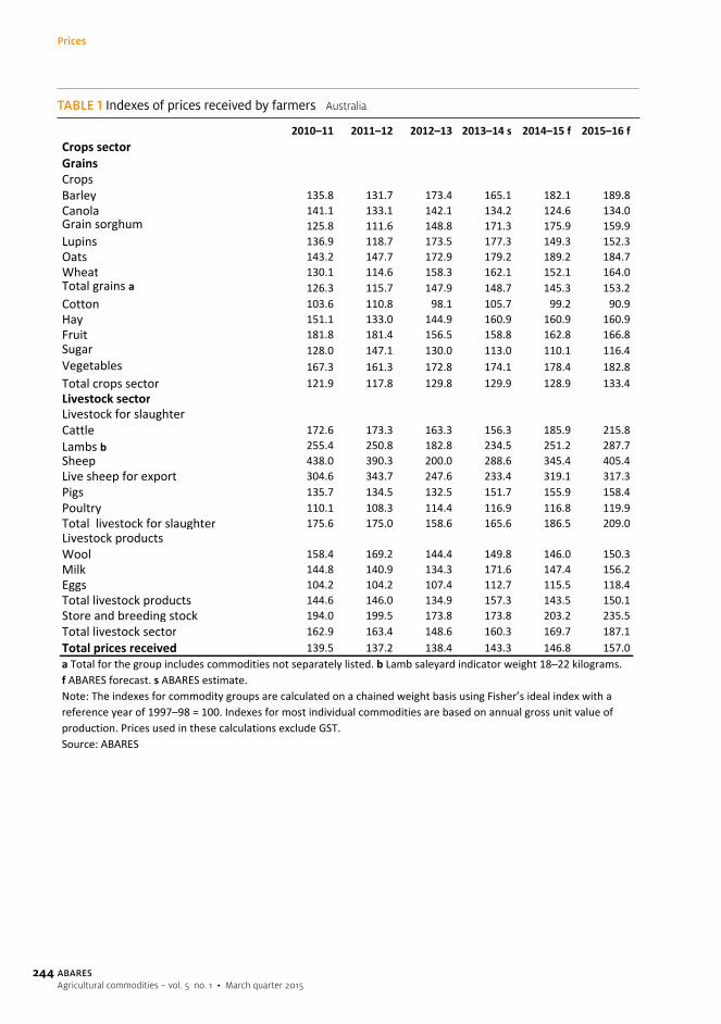
244 ABARESAgricultural commodities – vol. 5 no. 1 • March quarter 2015
TABLE 1 Indexes of prices received by farmers Australia
STATISTICS
2010–11 2011–12 2012–13 2013–14 s 2014–15 f 2015–16 f
Barley 135.8 131.7 173.4 165.1 182.1 189.8Canola 141.1 133.1 142.1 134.2 124.6 134.0Grain sorghum 125.8 111.6 148.8 171.3 175.9 159.9Lupins 136.9 118.7 173.5 177.3 149.3 152.3Oats 143.2 147.7 172.9 179.2 189.2 184.7Wheat 130.1 114.6 158.3 162.1 152.1 164.0Total grains a 126.3 115.7 147.9 148.7 145.3 153.2Cotton 103.6 110.8 98.1 105.7 99.2 90.9Hay 151.1 133.0 144.9 160.9 160.9 160.9Fruit 181.8 181.4 156.5 158.8 162.8 166.8Sugar 128.0 147.1 130.0 113.0 110.1 116.4Vegetables 167.3 161.3 172.8 174.1 178.4 182.8Total crops sector 121.9 117.8 129.8 129.9 128.9 133.4
Cattle 172.6 173.3 163.3 156.3 185.9 215.8Lambs b 255.4 250.8 182.8 234.5 251.2 287.7Sheep 438.0 390.3 200.0 288.6 345.4 405.4Live sheep for export 304.6 343.7 247.6 233.4 319.1 317.3Pigs 135.7 134.5 132.5 151.7 155.9 158.4Poultry 110.1 108.3 114.4 116.9 116.8 119.9Total livestock for slaughter 175.6 175.0 158.6 165.6 186.5 209.0
Wool 158.4 169.2 144.4 149.8 146.0 150.3Milk 144.8 140.9 134.3 171.6 147.4 156.2Eggs 104.2 104.2 107.4 112.7 115.5 118.4Total livestock products 144.6 146.0 134.9 157.3 143.5 150.1Store and breeding stock 194.0 199.5 173.8 173.8 203.2 235.5Total livestock sector 162.9 163.4 148.6 160.3 169.7 187.1Total prices received 139.5 137.2 138.4 143.3 146.8 157.0a Total for the group includes commodities not separately listed. b Lamb saleyard indicator weight 18–22 kilograms. f ABARES forecast. s ABARES estimate.Note: The indexes for commodity groups are calculated on a chained weight basis using Fisher’s ideal index with a reference year of 1997–98 = 100. Indexes for most individual commodities are based on annual gross unit value of production. Prices used in these calculations exclude GST.Source: ABARES
Livestock products
Livestock sector
1IndexesofpricesreceivedbyfarmersAustraliaCrops sector GrainsCrops
Livestock for slaughter
Prices

245ABARESAgricultural commodities – vol. 5 no. 1 • March quarter 2015
TABLE 2 Indexes of prices paid by farmers, and terms of trade Australia
STATISTICS
2 d f d b f d f d2Indexesofpricespaidbyfarmers,andtermsoftradeAustralia2Indexesofpricespaidbyfarmers,andtermsoftradeAustralia2010–11 2011–12 2012–13 2013–14 s 2014–15 f 2015–16 f2010 11 2011 12 2012 13 2013 14 s 2014 15 f 2015 16 f
Farmers’ terms of trade a 96 3 93 2 95 3 98 4 100 3 105 1Farmers’ terms of trade a 96.3 93.2 95.3 98.4 100.3 105.1Materials and servicesMaterials and servicesS d f dd d li t kSeed, fodder and livestock Fodder and feedstuffs 121.2 115.6 127.0 126.4 134.0 139.5 Fodder and feedstuffs 121.2 115.6 127.0 126.4 134.0 139.5Seed, seedlings and plants 120.0 116.4 128.0 130.0 130.2 135.4 Seed, seedlings and plants 120.0 116.4 128.0 130.0 130.2 135.4Store and breeding stock 194 0 199 5 173 8 173 8 203 2 235 5 Store and breeding stock 194.0 199.5 173.8 173.8 203.2 235.5Total seed fodder and livestock 137 8 135 1 138 0 137 7 149 5 160 8 Total seed, fodder and livestock 137.8 135.1 138.0 137.7 149.5 160.8Ch i lChemicals 110.4 112.6 110.3 113.6 114.7 118.1Electricity 158.8 176.7 180.8 185.5 176.2 180.7Electricity 158.8 176.7 180.8 185.5 176.2 180.7Fertiliser 157.3 165.5 157.9 153.2 154.7 159.4Fertiliser 157.3 165.5 157.9 153.2 154.7 159.4Fuel and lubricants 211 3 228 2 216 8 221 1 189 8 161 4Fuel and lubricants 211.3 228.2 216.8 221.1 189.8 161.4Total 146 0 149 2 149 5 151 0 154 1 158 3Total 146.0 149.2 149.5 151.0 154.1 158.3Marketing 144.8 154.1 153.6 159.2 151.4 144.2gOverheadsInsurance 173 7 185 8 190 0 195 0 199 8 204 8OverheadsInsurance 173.7 185.8 190.0 195.0 199.8 204.8Interest paid 122 3 114 9 96 4 85 3 79 7 83 4Interest paid 122.3 114.9 96.4 85.3 79.7 83.4R d 149 4 153 0 156 4 160 5 164 5 168 6Rates and taxes 149.4 153.0 156.4 160.5 164.5 168.6Other overheads 143.9 147.3 151.8 155.7 159.6 163.6Other overheads 143.9 147.3 151.8 155.7 159.6 163.6Total 133.6 129.8 117.6 110.6 107.5 111.5Total 133.6 129.8 117.6 110.6 107.5 111.5Capital items 149 3 153 2 157 0 161 4 165 7 170 1Capital items 149.3 153.2 157.0 161.4 165.7 170.1Total prices paid 144 8 147 2 145 2 145 6 146 4 149 4Total prices paid 144.8 147.2 145.2 145.6 146.4 149.4Excluding capital items 144.4 146.6 144.0 144.0 144.5 147.4g pExcluding capital and overheads 147.1 151.3 151.9 154.4 156.0 158.5Excluding capital and overheads 147.1 151.3 151.9 154.4 156.0 158.5Excluding seed, fodder andstore and breeding stock 146 2 149 7 146 6 147 2 145 6 146 8Excluding seed, fodder and store and breeding stock 146.2 149.7 146.6 147.2 145.6 146.8a Ratio of index of prices received by farmers and index of prices paid by farmers. f ABARES forecast. s ABARES p y p p yestimate.estimate.Note: The indexes for commodity groups are calculated on a chained weight basis using Fisher’s ideal index with aNote: The indexes for commodity groups are calculated on a chained weight basis using Fisher’s ideal index with a f f 1997 98 100 P i d i th l l ti l d GSTreference year of 1997–98 = 100. Prices used in these calculations exclude GST.
Sources: ABARES (compiled from various market sources); Australian Bureau of StatisticsSources: ABARES (compiled from various market sources); Australian Bureau of Statistics
Prices

246 ABARESAgricultural commodities – vol. 5 no. 1 • March quarter 2015
TABLE 3 Farm costs and returns Australia
STATISTICS
unit 2010–11 2011–12 2012–13 2013–14 s 2014–15 f 2015–16 f
Chemicals $m 1 462 1 471 1 429 1 461 1 482 1 534Fertiliser $m 2 248 2 344 2 237 2 141 2 146 2 214Fuel and lubricants $m 2 254 2 407 2 288 2 283 1 921 1 624Marketing $m 3 837 3 998 3 842 4 255 4 068 4 162Repairs and maintenance $m 3 659 3 878 4 106 4 670 4 703 5 138Seed and fodder $m 4 213 4 131 4 640 4 616 4 910 5 206Other $m 4 261 4 426 4 555 4 770 4 716 4 814Total materials and services $m 21 935 22 655 23 096 24 196 23 946 24 692Labour $m 4 145 4 174 4 344 4 345 4 310 4 397
Interest paid $m 5 023 4 836 4 259 3 956 3 883 4 267Rent and third party insurance $m 513 525 537 551 565 579Total overheads $m 9 680 9 536 9 140 8 852 8 758 9 242Total cash costs $m 31 615 32 191 32 236 33 048 32 703 33 934Depreciation a $m 4 944 5 072 5 199 5 342 5 485 5 632Total farm costs $m 36 559 37 263 37 435 38 390 38 188 39 566
Gross value of farm production $m 46 375 47 432 48 501 53 149 51 631 54 380
Net value of farm production b $m 9 816 10 169 11 066 14 759 13 443 14 814Real net value of farm production c $m 10 808 10 942 11 646 15 122 13 443 14 453Net farm cash income d $m 14 759 15 241 16 265 20 101 18 927 20 446Real net farm cash income c $m 16 252 16 400 17 117 20 595 18 927 19 947
3FarmcostsandreturnsAustralia
a Based on estimated movements in capital expenditure and prices of capital inputs. b Gross value of farm production less total farm costs. c In 2014–15 Australian dollars. d Gross farm cash income less total cash costs. f ABARES forecast. s ABARES estimate.Note: Prices used in these calculations exclude GST.Sources: ABARES (compiled from various market sources); Australian Bureau of Statistics
Costs Materials and services
Overheads
Returns
Net returns and production
Costs and returns

247ABARESAgricultural commodities – vol. 5 no. 1 • March quarter 2015
Exports
FIGURE 5 Contribution to exports by sector, balance of payments basis Australia
2011–12
2012–13
2009–10
2010–11
Othermerchandise
18%
Rural a15%
Mineralresources
67%
Othermerchandise
14%
Rural a15%
Mineralresources
71%
Mineralresources
69%
Rural a16%
Othermerchandise
15%
Services18%
Rural a13%
Othermerchandise
12%
Mineralresources57%
Services 16%
Rural a12%
Othermerchandise
13%
Mineralresources59%
Services17%
Rural a12%
Othermerchandise
13%
Mineralresources58%
Services20%
Rural a12%
Othermerchandise
15%
Mineralresources53%
Othermerchandise
15%
Rural a14%
Mineralresources
71%
Proportion ofmerchandise exports
Proportion of exportsof goods and services
a ABARES rural balance of payments adjusted to include farm, fisheries and forestry products classified as other merchandise by Australian Bureau of Statistics.Sources: ABARES; Australian Bureau of Statistics
2013–14
Mineralresources
70%
Rural a16%
Othermerchandise
14%
Services17%
Rural a13%
Othermerchandise
12%
Mineralresources58%

248 ABARESAgricultural commodities – vol. 5 no. 1 • March quarter 2015
TABLE 5 Industry gross value added a, b Australia
STATISTICS
5 d l dd d5Industrygrossvalueaddeda,bAustralia5Industrygrossvalueaddeda,bAustraliaunit 2008–09 2009–10 2010–11 2011–12 2012–13 2013–14unit 2008 09 2009 10 2010 11 2011 12 2012 13 2013 14
Agriculture forestry and fishingAgric lt re $ 29 432 29 141 30 324 30 671 30 443 32 005Agriculture, forestry and fishingAgriculture $m 29 432 29 141 30 324 30 671 30 443 32 005
d f h $Forestry and fishing $m 4 298 4 278 4 291 4 419 4 427 4 342y g $Total $m 33 747 33 442 34 601 35 086 34 869 36 348Total $m 33 747 33 442 34 601 35 086 34 869 36 348Mining $m 91 329 98 421 100 304 107 751 117 019 128 557Mining $m 91 329 98 421 100 304 107 751 117 019 128 557Manufacturing
d b d l h l $ManufacturingFood, beverage and alcohol $m 23 598 24 336 24 312 24 808 25 325 25 385, gTextile, clothing, footwearTextile, clothing, footwearand leather $m 7 187 5 878 5 667 5 436 5 372 5 537 and leather $m 7 187 5 878 5 667 5 436 5 372 5 537
Wood and paper products $m 6 744 6 917 6 508 6 003 5 988 6 092Wood and paper products $m 6 744 6 917 6 508 6 003 5 988 6 092Printin p blishinPrinting, publishing
d d d d $ and recorded media $m 4 468 4 112 4 106 3 678 3 622 3 423$Petroleum, coal, chemical products $m 17 512 18 186 18 195 18 696 17 410 16 327Petroleum, coal, chemical products $m 17 512 18 186 18 195 18 696 17 410 16 327Non‐metallic mineral products $m 6 483 6 382 6 275 5 892 5 858 5 928Non‐metallic mineral products $m 6 483 6 382 6 275 5 892 5 858 5 928Metal products $m 17 448 16 700 17 456 17 846 16 418 16 726Metal products $m 17 448 16 700 17 456 17 846 16 418 16 726M hi d i t $ 19 984 21 237 20 804 21 765 21 545 20 202Machinery and equipment $m 19 984 21 237 20 804 21 765 21 545 20 202
$Total manufacturing $m 103 126 103 573 103 356 104 201 101 538 99 619g $Building and construction $m 102 080 102 602 105 490 117 226 119 722 124 181Building and construction $m 102 080 102 602 105 490 117 226 119 722 124 181Electricity, gas and water supply $m 41 370 41 782 42 926 43 197 43 481 42 227Electricity, gas and water supply $m 41 370 41 782 42 926 43 197 43 481 42 227Taxes less subsidies on products $m 92 664 92 201 94 767 96 363 97 471 97 427Taxes less subsidies on products $m 92 664 92 201 94 767 96 363 97 471 97 427St ti ti l di $ 0 0 0 1 0 1 188Statistical discrepancy $m 0 0 0 1 0 1 188Gross domestic product $m 1 370 999 1 397 902 1 430 355 1 483 675 1 520 944 1 558 445Gross domestic product $a Chain volume measures, reference year is 2012–13. b ANZSIC 2006.a Chain volume measures, reference year is 2012 13. b ANZSIC 2006.Note: Zero is used to denote nil or less than $0 5 millionNote: Zero is used to denote nil or less than $0.5 million.S A t li B f St ti ti A t li ti l t ti l i dit d d t tSource: Australian Bureau of Statistics, Australian national accounts: national income, expenditure and product, cat. no. 5206.0, Canberra,
TABLE 4 Volume of production indexes Australia
STATISTICS
4 l f d d l4VolumeofproductionindexesAustralia4VolumeofproductionindexesAustraliaunit 2010–11 2011–12 2012–13 2013–14 s 2014–15 f 2015–16 funit 2010 11 2011 12 2012 13 2013 14 s 2014 15 f 2015 16 f
FarmGrains and oilseeds i d 139 9 158 6 138 4 151 8 134 5 135 9FarmGrains and oilseeds index 139.9 158.6 138.4 151.8 134.5 135.9
lTotal crops index 123.3 135.1 133.0 139.7 126.6 129.0pLivestock slaughterings index 110.4 110.2 116.1 127.5 129.5 123.4Livestock slaughterings index 110.4 110.2 116.1 127.5 129.5 123.4Total livestock index 100.6 100.7 104.7 111.1 112.2 108.1Total livestock index 100.6 100.7 104.7 111.1 112.2 108.1Total farm sector index 112 8 118 5 119 5 126 1 120 2 119 2Total farm sector index 112.8 118.5 119.5 126.1 120.2 119.2ForestryForestry aHardwood index 113.9 94.1 91.6 109.0 111.1 114.2Hardwood index 113.9 94.1 91.6 109.0 111.1 114.2Softwood index 136.0 126.6 122.9 130.3 134.5 135.5Softwood index 136.0 126.6 122.9 130.3 134.5 135.5Total forestry index 125 4 111 1 107 9 120 1 123 3 125 3Total forestry index 125.4 111.1 107.9 120.1 123.3 125.3a Vol me of logs har ested e cl ding fire ood f ABARES forecast s ABARES estimatea Volume of logs harvested excluding firewood. f ABARES forecast. s ABARES estimate.Note: ABARE revised the method for calculating production indexes in October 1999. The indexes for the different groups g p g pof commodities are calculated on a chained weight basis using Fisher’s ideal index with a reference year of 1997–98 = 100. of commodities are calculated on a chained weight basis using Fisher s ideal index with a reference year of 1997 98 = 100. Sources: ABARES; Australian Bureau of StatisticsSources: ABARES; Australian Bureau of Statistics
Sectors

249ABARESAgricultural commodities – vol. 5 no. 1 • March quarter 2015
TABLE 6 Employment a, b Australia
STATISTICS
6 l l6EmploymentAustraliaa,bAustralia6EmploymentAustraliaa,bAustralia2008–09 2009–10 2010–11 2011–12 2012–13 2013–142008 09 2009 10 2010 11 2011 12 2012 13 2013 14
’000 ’000 ’000 ’000 ’000 ’000’000 ’000 ’000 ’000 ’000 ’000Agriculture forestry and fishingA i lt 311 308 294 277 261 271Agriculture, forestry and fishingAgriculture 311 308 294 277 261 271Forestry and logging 7 7 5 8 6 6Forestry and logging 7 7 5 8 6 6Commercial fishing c 9 12 12 11 9 9Commercial fishing c 9 12 12 11 9 9Support services 23 25 26 25 25 27Support services 23 25 26 25 25 27T lTotal 350 351 337 321 302 313Mining 169 171 203 247 266 269Mining 169 171 203 247 266 269ManufacturingFood beverages and tobacco 221 220 220 219 216 223Manufacturing Food, beverages and tobacco 221 220 220 219 216 223Textiles, clothing, footwearTextiles, clothing, footwear
and leather 48 46 44 39 40 37 and leather 48 46 44 39 40 37Wood and paper product 66 63 56 54 52 62Wood and paper product 66 63 56 54 52 62Printing publishingPrinting, publishing
d d d di 2 and recorded media 51 52 55 41 47 41Petroleum, coalPetroleum, coal
and chemical product 89 87 84 88 90 85 and chemical product 89 87 84 88 90 85Non‐metallic mineral product 39 36 36 37 35 35Non‐metallic mineral product 39 36 36 37 35 35Metal product 154 143 143 144 127 138Metal product 154 143 143 144 127 138h f iOther manufacturing 346 339 332 318 328 309g
Total manufacturing 1 014 987 970 938 935 930Total manufacturing 1 014 987 970 938 935 930Other industries 9 226 9 336 9 605 9 743 9 886 9 971Other industries 9 226 9 336 9 605 9 743 9 886 9 971Total 10 758 10 846 11 115 11 249 11 389 11 482Total 10 758 10 846 11 115 11 249 11 389 11 482A l t f t b ANZSIC 2006 I l d lt fi hi h ti d t ia Average employment over four quarters. b ANZSIC 2006. c Includes aquaculture, fishing, hunting and trapping.
Note: Caution should be used when using employment statistics at the ANZSIC subdivision and group levels due to g p y g pestimates that may be subject to sampling variability and standard errors too high for most practical purposes.estimates that may be subject to sampling variability and standard errors too high for most practical purposes. Source: Australian Bureau of Statistics Labour force Australia cat no 6291 0 55 003 CanberraSource: Australian Bureau of Statistics, Labour force, Australia, cat. no. 6291.0.55.003, Canberra
TABLE 7 All banks lending to business a Australia
2014–152013–142012–13 2014 15Dec Mar Jun Sep Dec Mar Jun Sep
2013 142012 13Dec Mar Jun Sep Dec Mar Jun Sep$b $b $b $b $b $b $b $b$b $b $b $b $b $b $b $b
i l f d fi hiAgriculture, forestry and fishing 58.7 58.1 60.7 60.0 58.3 58.5 60.7 62.1g , y gMining 18.1 18.8 21.0 24.1 25.9 26.5 28.7 31.3Mining 18.1 18.8 21.0 24.1 25.9 26.5 28.7 31.3Manufacturing 39.7 39.5 39.6 38.7 38.0 41.8 43.1 39.7Manufacturing 39.7 39.5 39.6 38.7 38.0 41.8 43.1 39.7Construction 27 6 27 8 27 5 27 8 27 7 28 4 28 5 28 6Construction 27.6 27.8 27.5 27.8 27.7 28.4 28.5 28.6Wholesale and retail trade
d 102 3 102 2 103 0 104 1 103 1 105 3 101 8 102 9Wholesale and retail trade, transport and storage 102.3 102.2 103.0 104.1 103.1 105.3 101.8 102.9p gFinance and insurance 103.0 104.2 107.2 112.3 122.8 124.8 131.2 135.0Finance and insurance 103.0 104.2 107.2 112.3 122.8 124.8 131.2 135.0Other 344.5 347.1 351.3 352.8 354.5 357.6 370.8 377.1Other 344.5 347.1 351.3 352.8 354.5 357.6 370.8 377.1Total 694 0 697 7 710 4 719 8 730 4 742 8 764 9 776 6Total 694.0 697.7 710.4 719.8 730.4 742.8 764.9 776.6I l d i bl d fi d i t t t l t t di l b k bill t t dia Includes variable and fixed interest rate loans outstanding plus bank bills outstanding.
Source: Reserve Bank of Australia, Bank lending to business – selected statistics, Bulletin Statistical Table D8Source: Reserve Bank of Australia, Bank lending to business selected statistics, Bulletin Statistical Table D8
Employment, banks
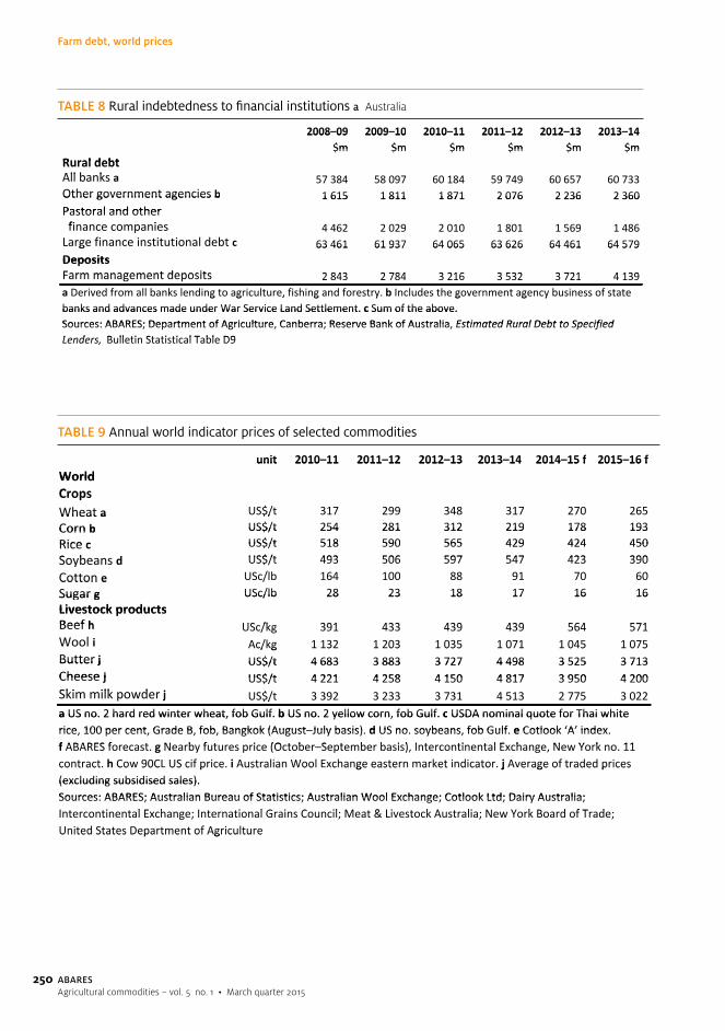
250 ABARESAgricultural commodities – vol. 5 no. 1 • March quarter 2015
TABLE 8 Rural indebtedness to financial institutions a Australia
STATISTICS
8 l d b d f l8RuralindebtednesstofinancialinstitutionsAustralia8RuralindebtednesstofinancialinstitutionsAustralia2008–09 2009–10 2010–11 2011–12 2012–13 2013–142008 09 2009 10 2010 11 2011 12 2012 13 2013 14
$m $m $m $m $m $m$m $m $m $m $m $mRural debtAll b kRural debtAll banks a 57 384 58 097 60 184 59 749 60 657 60 733Other government agencies b 1 615 1 811 1 871 2 076 2 236 2 360Other government agencies b 1 615 1 811 1 871 2 076 2 236 2 360Pastoral and otherfi iPastoral and other finance companies 4 462 2 029 2 010 1 801 1 569 1 486Large finance institutional debt c 63 461 61 937 64 065 63 626 64 461 64 579g 63 461 61 937 64 065 63 626 64 461 64 579DepositsFarm management deposits 2 843 2 784 3 216 3 532 3 721 4 139DepositsFarm management deposits 2 843 2 784 3 216 3 532 3 721 4 139a Derived from all banks lending to agriculture, fishing and forestry. b Includes the government agency business of state g g , g y g g ybanks and advances made under War Service Land Settlement. c Sum of the above.banks and advances made under War Service Land Settlement. c Sum of the above.Sources: ABARES; Department of Agriculture Canberra; Reserve Bank of Australia Estimated Rural Debt to SpecifiedSources: ABARES; Department of Agriculture, Canberra; Reserve Bank of Australia, Estimated Rural Debt to Specified L d B ll ti St ti ti l T bl D9Lenders, Bulletin Statistical Table D9
TABLE 9 Annual world indicator prices of selected commodities
STATISTICS
9 l ld d f l d d9Annualworldindicatorpricesofselectedcommodities9Annualworldindicatorpricesofselectedcommoditiesunit 2010–11 2011–12 2012–13 2013–14 2014–15 f 2015–16 funit 2010 11 2011 12 2012 13 2013 14 2014 15 f 2015 16 f
WorldWorldCropsCropsWheat a US$/t 317 299 348 317 270 265Wheat a $/Corn b US$/t 254 281 312 219 178 193Corn b US$/t 254 281 312 219 178 193Rice c US$/t 518 590 565 429 424 450Rice c US$/t 518 590 565 429 424 450S b d US$/t 493 506 597 547 423 390Soybeans d US$/t 493 506 597 547 423 390
/Cotton e USc/lb 164 100 88 91 70 60Cotton e /Sugar g USc/lb 28 23 18 17 16 16Sugar g USc/lb 28 23 18 17 16 16Livestock productsBeef h US /k 391 433 439 439 564 571Livestock productsBeef h USc/kg 391 433 439 439 564 571W lWool i Ac/kg 1 132 1 203 1 035 1 071 1 045 1 075Ac/kg 1 132 1 203 1 035 1 071 1 045 1 075Butter j US$/t 4 683 3 883 3 727 4 498 3 525 3 713Butter j US$/t 4 683 3 883 3 727 4 498 3 525 3 713Cheese j US$/t 4 221 4 258 4 150 4 817 3 950 4 200Cheese j US$/t 4 221 4 258 4 150 4 817 3 950 4 200Ski ilk d j $Skim milk powder j US$/t 3 392 3 233 3 731 4 513 2 775 3 022$/a US no. 2 hard red winter wheat, fob Gulf. b US no. 2 yellow corn, fob Gulf. c USDA nominal quote for Thai white a US no. 2 hard red winter wheat, fob Gulf. b US no. 2 yellow corn, fob Gulf. c USDA nominal quote for Thai white rice 100 per cent Grade B fob Bangkok (August–July basis) d US no soybeans fob Gulf e Cotlook ‘A’ indexrice, 100 per cent, Grade B, fob, Bangkok (August–July basis). d US no. soybeans, fob Gulf. e Cotlook ‘A’ index. f ABARES f t N b f t i (O t b S t b b i ) I t ti t l E h N Y k 11f ABARES forecast. g Nearby futures price (October–September basis), Intercontinental Exchange, New York no. 11 contract. h Cow 90CL US cif price. i Australian Wool Exchange eastern market indicator. j Average of traded prices co t act Co 90C US c p ce ust a a oo c a ge easte a et d cato j e age o t aded p ces(excluding subsidised sales).(excluding subsidised sales).Sources: ABARES; Australian Bureau of Statistics; Australian Wool Exchange; Cotlook Ltd; Dairy Australia;Sources: ABARES; Australian Bureau of Statistics; Australian Wool Exchange; Cotlook Ltd; Dairy Australia; I t ti t l E h I t ti l G i C il M t & Li t k A t li N Y k B d f T dIntercontinental Exchange; International Grains Council; Meat & Livestock Australia; New York Board of Trade; United States Department of Agriculture United States Department of Agriculture
Farm debt, world prices

251ABARESAgricultural commodities – vol. 5 no. 1 • March quarter 2015
TABLE 10 Gross unit values of farm products a
STATISTICS
10 l f f d10Grossunitvaluesoffarmproductsa10Grossunitvaluesoffarmproductsaunit 2010–11 2011–12 2012–13 2013–14 s 2014–15 f 2015–16 funit 2010 11 2011 12 2012 13 2013 14 s 2014 15 f 2015 16 f
Crops bCrops bGrainsGrains
l $/Barley $/t 216 210 276 263 290 302y $/Corn (maize) $/t 259 251 238 253 239 233Corn (maize) $/t 259 251 238 253 239 233Grain sorghum $/t 213 189 252 290 298 271Grain sorghum $/t 213 189 252 290 298 271Oats $/t 196 202 236 245 259 252Oats $/t 196 202 236 245 259 252Ri $/t 240 270 260 326 409 402Rice $/t 240 270 260 326 409 402Triticale $/t 184 176 249 247 244 235Triticale $/Wheat $/t 257 227 313 321 301 324Wheat $/t 257 227 313 321 301 324OilseedsOilseedsCanola $/t 544 513 548 518 481 517Canola $/t 544 513 548 518 481 517Soybeans c $/ 501 472 442 464 473 492Soybeans c $/t 501 472 442 464 473 492Sunflower seed c $/t 567 551 570 712 651 651Sunflower seed c $/t 567 551 570 712 651 651PulsesPulsesChickpeas $/t 404 457 394 351 413 368Chickpeas $/t 404 457 394 351 413 368Field peas $/t 266 295 406 423 413 421Field peas $/t 266 295 406 423 413 421L i $/Lupins $/t 268 232 340 347 292 298pIndustrial cropsIndustrial cropsCotton lint d c/kg 377 225 199 229 196 183Cotton lint d c/kg 377 225 199 229 196 183Sugar cane (cut for crushing) $/t 38 43 41 36 36 39Sugar cane (cut for crushing) $/t 38 43 41 36 36 39Wi $/ 413 458 499 441 459 466Wine grapes $/t 413 458 499 441 459 466g pLivestockLivestockBeef cattle c/kg 336 337 318 304 362 420Beef cattle c/kg 336 337 318 304 362 420Lambs c/kg 519 509 371 476 510 584Lambs c/kg 519 509 371 476 510 584Pigs c/kg 269 266 262 300 309 314Pigs c/kg 269 266 262 300 309 314
l /Poultry c/kg 197 194 205 209 209 215y / gLivestock productsLivestock productsWool c/kg 623 666 568 589 574 591Wool c/kg 623 666 568 589 574 591Milk c/L 43 42 40 51 44 47Milk c/L 43 42 40 51 44 47A it l ll d i i i l k t l th i i di t d I l d th t fa Average gross unit value across all grades in principal markets, unless otherwise indicated. Includes the cost of
containers, commission and other expenses incurred in getting the commodities to their principal markets. These co ta e s, co ss o a d ot e e pe ses cu ed gett g t e co od t es to t e p c pa a ets eseexpenses are significant. b Average unit gross value relates to returns received from crops harvested in that year,expenses are significant. b Average unit gross value relates to returns received from crops harvested in that year, regardless of when sales take place unless otherwise indicated c Price paid by crusher d Australian base price forregardless of when sales take place, unless otherwise indicated. c Price paid by crusher. d Australian base price for l i th fi i l i di t d f ABARES f t ABARES ti tsales in the financial year indicated. f ABARES forecast. s ABARES estimate.
Note: Prices used in these calculations exclude GST.Note: Prices used in these calculations exclude GST.Sources: ABARES; Australian Bureau of StatisticsSources: ABARES; Australian Bureau of Statistics
Gross unit values

252 ABARESAgricultural commodities – vol. 5 no. 1 • March quarter 2015
World
TABLE 11 World production, consumption, stocks and trade for selected commodities a
STATISTICS
unit 2010–11 2011–12 2012–13 2013–14 2014–15 f 2015–16 f
production Mt 653 695 655 713 720 707 consumption Mt 657 698 677 696 713 707 closing stocks Mt 194 191 169 185 192 192 exports bc Mt 126 145 141 155 151 147
production Mt 1 099 1 157 1 136 1 280 1 273 1 248 consumption Mt 1 129 1 137 1 142 1 230 1 255 1 263 closing stocks Mt 166 165 169 210 229 214 exports b Mt 116 147 123 163 151 152
production d Mt 449 467 472 475 475 485 consumption d Mt 445 458 469 478 482 489 closing stocks d Mt 100 108 112 109 102 98 exports be Mt 36 39 39 42 42 40
production Mt 461 447 475 505 530 522 consumption Mt 448 466 468 488 505 514 closing stocks Mt 84 65 67 81 106 113 exports Mt 108 111 118 134 134 136
production Mt 149 157 161 170 175 180 consumption Mt 145 152 158 166 176 179 closing stocks Mt 15 17 17 21 20 22 exports Mt 61 65 68 68 72 76
production Mt 257 267 268 280 292 300 consumption Mt 252 263 264 275 287 297 closing stocks Mt 11 12 11 16 21 24 exports Mt 77 80 78 82 84 87
production Mt 26 28 27 26 26 25 consumption Mt 25 23 23 24 25 25 closing stocks Mt 11 16 20 22 23 23 exports Mt 8 10 10 9 7 7
production Mt 166 175 185 183 183 184 consumption Mt 164 169 176 179 183 184 closing stocks Mt 59 65 74 78 78 78 exports Mt 55 56 61 58 59 61
continued...
11Worldproduction,consumption,stocksandtradeforselectedcommodities
Vegetable protein meals
Grains
Cotton
Sugar
Farm
Oilseeds and vegetable oils
Industrial crops
Wheat
Coarse grains
Rice
Oilseeds
Vegetable oils

253ABARESAgricultural commodities – vol. 5 no. 1 • March quarter 2015
World
TABLE 11 World production, consumption, stocks and trade for selected commodities a continued
STATISTICS
unit 2010–11 2011–12 2012–13 2013–14 2014–15 f 2015–16 f
production Mt 262 268 272 276 272 274 consumption Mt 258 264 268 271 267 273 closing stocks Mt 2.1 2.5 2.5 2.4 2.0 2.6 exports b Mt 26.1 27.2 28.1 28.9 29.2 29.7
production kt 1 117 1 133 1 159 1 131 1 132 1 132 consumption ej kt 1 130 1 110 1 105 1 127 1 130 1 135 closing stocks k kt 45 24 25 35 35 30 exports l kt 502 447 485 496 490 480
production kt 8 584 8 914 9 150 9 440 9 760 na consumption kt 8 105 8 431 8 671 8 869 9 184 na closing stocks kt 213 247 231 242 243 na exports kt 724 762 815 862 865 naSkim milk powder ehm production kt 3 675 3 983 3 953 4 371 4 421 na consumption kt 3 192 3 447 3 482 3 606 3 791 na closing stocks kt 452 431 385 459 412 na exports kt 1 529 1 627 1 663 1 823 1 872 na
11Worldproduction,consumption,stocksandtradeforselectedcommodities
a Some figures are not based on precise or complete analyses. b Excludes intra‐EU trade. c Includes the grain equivalent of wheat flour. d Milled equivalent. e On a calendar year basis, e.g. 2011–12 = 2012. f ABARES forecast. g Beef and veal, mutton, lamb, goat, pig and poultry meat. h Selected countries. i Clean equivalent. j Virgin wool at the spinning stage in 65 countries. k Held by marketing bodies and on‐farm in five major exporting countries. l Five major exporting countries. m Non‐fat dry milk. na Not available.Sources: ABARES; Argentine Wool Federation; Australian Bureau of Statistics; Capewools South Africa; Commonwealth Secretariat; Department of Agriculture, Canberra; Economic Commission for Europe; Fearnleys; Food and Agriculture Organization; International Grains Council; International Sugar Organization; International Wool Textile Organisation; ISTA Mielke and Co; Ministry of Agriculture, Forestry and Fisheries (Japan); New Zealand Wool Board; Poimena Analysis, Melbourne; United States Department of Agriculture; Uruguayan Association of Wool Exporters
Livestock products Meat egh
Wool i
Butter eh

254 ABARESAgricultural commodities – vol. 5 no. 1 • March quarter 2015
Australian production
TABLE 12 Agricultural, fisheries and forestry commodity production Australia
STATISTICS
unit 2010–11 2011–12 2012–13 2013–14 s 2014–15 f 2015–16 fCropsGrainsBarley kt 7 995 8 221 7 472 9 669 7 954 7 490Corn (maize) kt 357 451 507 340 374 383Grain sorghum kt 1 935 2 239 2 230 1 107 1 790 1 869Oats kt 1 128 1 262 1 121 1 276 1 127 1 149Rice kt 723 919 1 161 833 684 794Triticale kt 355 285 171 274 248 266Wheat kt 27 410 29 905 22 856 26 929 23 607 24 390OilseedsCanola kt 2 359 3 427 4 142 3 795 3 413 3 264Cottonseed kt 1 269 1 732 1 439 1 252 665 791Soybeans kt 30 86 92 62 53 63Sunflower seed kt 43 47 44 32 31 35Other oilseeds a kt 33 35 35 47 42 33PulsesChickpeas kt 513 673 813 632 517 636Field peas kt 395 342 320 339 302 327Lupins kt 808 982 459 622 576 460Total grains, oilseeds and pulses kt 45 352 50 606 42 861 47 209 41 384 41 949Industrial cropsCotton lint kt 926 1 225 1 018 885 470 560Sugar cane (cut for crushing) kt 27 443 27 943 30 400 30 500 32 100 33 457Sugar (tonnes actual) kt 3 610 3 683 4 300 4 380 4 700 4 962Wine grapes kt 1 598 1 582 1 642 1 650 1 534 1 602HorticultureFruitApples kt 300 289 289 280 286 291Bananas kt 203 286 330 356 321 327Oranges kt 291 390 401 430 434 438VegetablesCarrots kt 225 319 272 290 297 304Onions kt 331 347 302 336 347 358Potatoes kt 1 128 1 288 1 273 1 234 1 229 1 225Tomatoes kt 302 372 456 410 411 413LivestockSlaughteringsCattle and calves ’000 8 097 7 873 8 457 9 473 9 475 8 900Lambs ’000 17 880 18 879 21 122 21 899 22 300 21 470Sheep ’000 5 341 5 175 8 192 10 066 9 200 6 197Pigs ’000 4 643 4 733 4 745 4 778 4 866 4 970Live exportsCattle exported live b ’000 805 683 634 1 133 1 120 1 000Sheep exported live c ’000 2 916 2 562 2 000 2 020 2 400 2 250Meat producedBeef and veal d kt 2 133 2 115 2 245 2 464 2 473 2 359Lamb d kt 391 419 457 474 488 466Mutton d kt 123 120 183 228 221 143Chicken meat d kt 1 015 1 030 1 046 1 084 1 125 1 160Pig meat kt 342 351 356 360 368 376Total kt 4 005 4 034 4 287 4 610 4 676 4 503
continued...
12Agricultural,fisheriesandforestrycommodityproductionAustralia

255ABARESAgricultural commodities – vol. 5 no. 1 • March quarter 2015
Australian production
TABLE 12 Agricultural, fisheries and forestry commodity production Australia continued
STATISTICS
12Agricultural,fisheriesandforestrycommodityproductionAustraliacontinuedunit 2010–11 2011–12 2012–13 2013–14 s 2014–15 f 2015–16 f
Wool e kt 429 411 435 431 417 399Milk g ML 9 100 9 480 9 201 9 239 9 405 9 590Butter h kt 122 120 118 116 117 119Cheese kt 339 347 338 311 330 335Casein kt 5 5 5 4 3 3Skim milk powder kt 222 230 224 211 220 224Whole milk powder kt 151 140 109 126 117 120Buttermilk powder kt 12 11 11 11 11 11
Hardwood ’000 m3 11 551 9 548 9 291 11 061 11 268 11 588Softwood ’000 m3 14 981 13 949 13 536 14 358 14 817 14 928Total ’000 m3 26 532 23 497 22 827 25 418 26 085 26 516
Tuna kt 9.1 10.1 11.4 11.5 12.7 12.7Salmonids k kt 36.8 44.2 43.0 41.6 45.1 47.4Other fish kt 112.9 113.1 105.6 110.5 109.7 108.6Prawns kt 27.2 22.5 21.1 25.2 23.0 24.9Rock lobster l kt 9.9 9.1 10.5 9.9 10.0 10.3Abalone m kt 5.2 5.1 5.3 5.0 4.9 4.6Scallops kt 7.0 3.6 6.8 5.0 5.9 6.1Oysters kt 13.9 12.6 12.5 12.8 13.0 13.8Other molluscs kt 6.6 7.9 7.9 6.7 6.5 6.6Other crustaceans kt 6.3 5.5 5.2 5.6 5.4 5.4
Livestock products
Forestry products i
Fisheries j
a Linseed, safflower seed and peanuts. b Includes all bovine for feeder/slaughter, breeding and dairy purposes. c Includes animals for breeding. d In carcass weight and includes carcass equivalent of canned meats. e Greasy equivalent of shorn wool (includes crutching), dead and fellmongered wool and wool exported on skins. f ABARES forecast. g Includes the whole milk equivalent of farm cream intake. h Includes the butter equivalent of butter oil, butter concentrate, ghee and dry butterfat. i Excludes logs harvested for firewood. j Liveweight. k Includes salmon and trout production. l Includes Queensland bugs. m Excludes Victorian aquaculture production for 2009–10 and 2010–11. s ABARES estimate.Sources: ABARES; Australian Bureau of Statistics; Australian Fisheries Management Authority; Dairy Australia; Department of Fisheries, Western Australia; Department of Primary Industries, Parks, Water and Environment, Tasmania; Fisheries Queensland, Department of Agriculture, Fisheries and Forestry; Fisheries Victoria, Department of Primary Industries; Industry & Investment New South Wales; Northern Territory Department of Regional Development, Primary Industry, Fisheries and Resources; Primary Industries and Regions, Fisheries, South Australia; Pulse Australia; Raw Cotton Marketing Advisory Committee; South Australian Research and Development Institute; state and territory forest services; various Australian forestry industries

256 ABARESAgricultural commodities – vol. 5 no. 1 • March quarter 2015
Value of production
TABLE 13 Gross value of farm, fisheries and forestry production Australia
STATISTICS
2010–11 2011–12 2012–13 2013–14 s 2014–15 f 2015–16 f$m $m $m $m $m $m
CropsGrainsBarley 1 729 1 723 2 063 2 541 2 306 2 264Corn (maize) 92 113 120 86 89 89Grain sorghum 412 423 562 321 533 506Oats 221 255 265 313 291 290Rice 174 248 302 272 279 319Triticale 65 50 43 68 61 62Wheat 7 052 6 775 7 154 8 631 7 100 7 908OilseedsCanola 1 283 1 759 2 270 1 964 1 640 1 687Soybeans 15 41 41 29 25 31Sunflower seed 24 26 25 23 20 23Other oilseeds a 30 33 27 23 20 23PulsesChickpeas 207 308 320 222 214 234Field peas 105 101 130 143 125 138Lupins 216 228 156 216 168 137Total grains, oilseeds and pulses 12 138 12 485 13 924 15 352 13 403 14 177Industrial cropsCotton lint and cottonseed b 2 087 2 954 2 174 2 036 1 015 1 108Sugar cane (cut for crushing) 1 036 1 214 1 253 1 109 1 160 1 294Wine grapes 712 725 858 728 703 746Total industrial crops 3 834 4 893 4 284 3 873 2 878 3 147HorticultureTable and dried grapes 302 316 303 347 295 379Fruit and nuts (excl. grapes) 3 013 3 050 3 662 3 590 3 919 3 869Vegetables 3 338 3 339 3 770 3 820 3 899 4 133Other horticulture 1 606 1 272 1 285 1 474 1 376 1 439Total horticulture 8 259 7 976 9 020 9 231 9 489 9 821Other crops nei c 1 105 898 1 165 1 545 1 345 1 345Total crops 25 336 26 251 28 394 30 001 27 116 28 490
continued...
13Grossvalueoffarm,fisheriesandforestryproductionAustralia

257ABARESAgricultural commodities – vol. 5 no. 1 • March quarter 2015
Value of production
TABLE 13 Gross value of farm, fisheries and forestry production Australia continued
2010–11 2011–12 2012–13 2013–14 s 2014–15 f 2015–16 f$m $m $m $m $m $m
Cattle and calves d 7 164 7 134 7 136 7 495 8 945 9 903Sheep e 484 419 329 590 684 519Lambs eg 2 029 2 136 1 696 2 258 2 491 2 722Pigs 919 934 934 1 081 1 137 1 180Poultry 2 077 2 078 2 214 2 344 2 435 2 577
Cattle exported live h 660 651 589 1 049 1 099 1 035Sheep exported live i 348 345 194 185 300 280Total livestock j 13 795 13 797 13 207 15 122 17 217 18 344
Wool k 2 673 2 734 2 472 2 537 2 392 2 360Milk l 3 932 3 986 3 687 4 730 4 138 4 469Eggs 572 583 653 670 690 625Honey and beeswax 66 79 88 88 78 92Total livestock products 7 243 7 383 6 900 8 026 7 298 7 546Total farm 46 375 47 432 48 501 53 149 51 631 54 380
Hardwood 892 742 685 829 847 880Softwood 959 879 835 970 1 011 1 028Total 1 851 1 620 1 520 1 799 1 857 1 908
Tuna 139 172 177 149 157 173Salmonids o 427 514 497 542 577 580Other fish q 432 456 441 466 438 437Prawns 308 266 277 359 339 367Rock lobster r 392 394 451 543 537 598Abalone t 178 170 190 160 163 153Scallops 22 8 15 11 14 15Oysters 97 90 95 96 100 105Pearls u 120 102 79 91 108 113Other molluscs v 32 33 59 31 42 46Other crustaceans 66 67 64 70 67 68Total fish 2 248 2 305 2 381 2 555 2 577 2 688a Linseed, safflower seed and peanuts. b Value delivered to gin. c Mainly fodder crops. d Includes dairy cattle slaughtered. e Excludes skin values. f ABARES forecast. g Lamb saleyard indicator weight 18–22 kilograms. h Includes all bovine for feeder/slaughter, breeding and dairy purposes. i Includes animals exported for breeding purposes. j Total livestock slaughterings includes livestock disposals. k Shorn, dead and fellmongered wool and wool exported on skins. l Milk intake by factories and valued at the farm gate. m Excludes logs harvested for firewood. n Value to fishers of product landed in Australia. o Includes salmon and trout production. q Includes an estimated value of aquaculture. r Includes Queensland bugs. s ABARES estimate. t Excludes Victorian aquaculture production for 2009–10 and 2010–11. u Northern Territory aquaculture production not included in 2012–13 due to confidentiality. v Also includes fish and aquaculture values not elsewhere included. nei Not elsewhere included.Note: The gross value of production is the value placed on recorded production at the wholesale prices realised in the marketplace. The point of measurement can vary between commodities. Generally the marketplace is the metropolitan market in each state and territory. However, where commodities are consumed locally or where they become raw material for a secondary industry, these points are presumed to be the marketplace. Prices used in these calculations exclude GST. Sources: ABARES; Australian Bureau of Statistics
Fisheries products n
13GrossvalueoffarmandfisheriesproductionAustraliacontinued
LivestockSlaughterings
Live exports
Livestock products
Forestry products m

258 ABARESAgricultural commodities – vol. 5 no. 1 • March quarter 2015
Areas, stock
TABLE 14 Crop and forestry areas and livestock numbers Australia
STATISTICS
unit 2010–11 2011–12 2012–13 2013–14 s 2014–15 f 2015–16 fCrop areasGrainsBarley ’000 ha 3 681 3 718 3 644 3 943 3 810 3 699Corn (maize) ’000 ha 62 70 79 58 66 66Grain sorghum ’000 ha 633 659 648 493 604 625Oats ’000 ha 826 731 729 723 718 750Rice ’000 ha 76 103 114 76 71 81Triticale ’000 ha 187 145 99 151 152 160Wheat ’000 ha 13 502 13 902 12 979 13 473 13 808 13 890OilseedsCanola ’000 ha 2 078 2 461 3 272 2 653 2 711 2 755Soybeans ’000 ha 17 38 41 31 27 31Sunflower seed ’000 ha 37 40 30 27 25 26Other oilseeds a ’000 ha 19 18 17 16 17 17PulsesChickpeas ’000 ha 653 456 574 507 425 530Field peas ’000 ha 318 249 281 245 231 250Lupins ’000 ha 756 689 450 387 437 400Total grains, oilseeds and pulses ’000 ha 23 946 24 295 23 841 23 567 23 728 23 939Industrial cropsCotton ’000 ha 590 600 442 392 210 250Sugar cane b ’000 ha 314 368 371 375 381 394Winegrapes c ’000 ha 154 145 133 138 142 143Livestock numbers dCattleBeef million 25.94 25.69 26.46 25.72 24.19 23.66Dairy million 2.57 2.73 2.83 2.73 2.78 2.82 Milking herd e million 1.59 1.70 1.69 1.69 1.69 1.70 Total million 28.51 28.42 29.29 28.46 26.96 26.48Sheep million 73.10 74.72 75.55 72.71 70.71 72.05Pigs million 2.29 2.14 2.10 2.00 1.96 1.91Forestry plantation areaHardwood ’000 ha 980 977 976 na na naSoftwood ’000 ha 1 025 1 024 1 024 na na naTotal plantation area g ’000 ha 2 017 2 013 2 013 na na na
14CropandforestryareasandlivestocknumbersAustralia
a Linseed and safflower seed. b Cut for crushing. c This figure is for grapes for wine only. Prior to 2008–09 this figure includes grapes used for winemaking and other purposes such as drying and table. d At 30 June. e Cows in milk and dry. f ABARES forecast. g Includes areas where plantation type is unknown. s ABARES estimate. na Not available.Sources: ABARES; Australian Bureau of Statistics; Pulse Australia

259ABARESAgricultural commodities – vol. 5 no. 1 • March quarter 2015
Yields
TABLE 15 Average farm yields Australia
STATISTICS
15 f ld l15AveragefarmyieldsAustralia15AveragefarmyieldsAustraliaunit 2010–11 2011–12 2012–13 2013–14 s 2014–15 f 2015–16 funit 2010 11 2011 12 2012 13 2013 14 s 2014 15 f 2015 16 f
CropsCropsGrainsGrainsB l /h 2 17 2 21 2 05 2 45 2 09 2 03Barley t/ha 2.17 2.21 2.05 2.45 2.09 2.03yCorn (maize) t/ha 5.74 6.47 6.44 5.88 5.69 5.81Corn (maize) t/haGrain sorghum t/ha 3.06 3.40 3.44 2.25 2.96 2.99Grain sorghum t/ha 3.06 3.40 3.44 2.25 2.96 2.99Oats t/ha 1.37 1.73 1.54 1.77 1.57 1.53Oats t/ha 1.37 1.73 1.54 1.77 1.57 1.53Rice t/ha 9 54 8 91 10 22 11 01 9 70 9 86Rice t/ha 9.54 8.91 10.22 11.01 9.70 9.86T i i l /h 1 90 1 97 1 73 1 81 1 64 1 66Triticale t/ha 1.90 1.97 1.73 1.81 1.64 1.66Wheat t/ha 2.03 2.15 1.76 2.00 1.71 1.76Wheat t/haOilseedsOilseedsCanola t/ha 1 14 1 39 1 27 1 43 1 26 1 19Canola t/ha 1.14 1.39 1.27 1.43 1.26 1.19So beans t/h 1 71 2 26 2 24 2 03 2 01 2 08Soybeans t/ha 1.71 2.26 2.24 2.03 2.01 2.08
fl d / 1 14 1 17 1 46 1 21 1 25 1 34Sunflower seed t/ha 1.14 1.17 1.46 1.21 1.25 1.34/PulsesPulsesChickpeas t/ha 0.79 1.48 1.42 1.25 1.22 1.20Chickpeas t/ha 0.79 1.48 1.42 1.25 1.22 1.20Field peas t/ha 1 24 1 38 1 14 1 39 1 31 1 31Field peas t/ha 1.24 1.38 1.14 1.39 1.31 1.31L i t/h 1 07 1 42 1 02 1 61 1 32 1 15Lupins t/ha 1.07 1.42 1.02 1.61 1.32 1.15Industrial cropspCotton (lint) t/ha 1.57 2.04 2.30 2.26 2.24 2.24Cotton (lint) t/ha 1.57 2.04 2.30 2.26 2.24 2.24Sugar cane (for crushing) t/ha 87 76 82 81 84 85Sugar cane (for crushing) t/ha 87 76 82 81 84 85Winegrapes t/ha 10 4 10 9 12 3 12 0 10 8 11 2Winegrapes t/ha 10.4 10.9 12.3 12.0 10.8 11.2Li t kLivestockWool a kg/sheep 4.34 4.19 4.41 4.37 4.43 4.40Wool a g/ pWhole milk L/cow 5 727 5 577 5 450 5 467 5 555 5 641Whole milk L/cow 5 727 5 577 5 450 5 467 5 555 5 641a Shorn (including lambs) f ABARES forecast s ABARES estimatea Shorn (including lambs). f ABARES forecast. s ABARES estimate.S ABARES A t li B f St ti ti P l A t liSources: ABARES; Australian Bureau of Statistics; Pulse Australia

260 ABARESAgricultural commodities – vol. 5 no. 1 • March quarter 2015
Export volumes
TABLE 16 Volume of agricultural and fisheries exports Australia
STATISTICS
unit 2010–11 2011–12 2012–13 2013–14 2014–15 f 2015–16 f
CropsGrainsBarley a kt 4 625 6 568 5 165 7 124 6 115 5 700Corn (maize) kt 12 68 134 83 55 97Grain sorghum kt 553 1 112 1 291 701 542 800Oats kt 127 163 200 237 258 268Rice kt 172 537 584 544 426 351Wheat b kt 18 431 23 026 21 265 18 336 16 944 17 946OilseedsCanola kt 1 471 2 323 3 488 3 194 2 382 2 432Cottonseed kt 268 654 754 464 235 200Other oilseeds c kt 7 6 10 14 8 8PulsesChickpeas kt 409 653 852 562 508 617Peas d kt 254 248 208 155 210 143Lupins kt 289 316 416 274 252 230Other pulses kt 485 775 691 795 466 485Total grains, oilseeds and pulses kt 27 104 36 448 35 058 32 483 28 402 29 277
Raw cotton e kt 505 994 1 305 1 036 730 483Sugar kt 2 735 2 572 3 004 3 052 3 361 3 594Wine ML 748 737 717 717 735 725Meat and live animalsBeef and veal g kt 937 948 1 014 1 184 1 223 1 158Live feeder/slaughter cattle h ’000 728 579 513 996 1 000 900Live breeder cattle i ’000 77 105 121 137 120 100Lamb g kt 157 174 201 226 240 215Live sheep j ’000 2 916 2 562 2 000 2 020 2 400 2 250Mutton g kt 86 89 144 183 172 108Pig meat g kt 31 29 26 27 28 28Poultry meat g kt 31 38 32 37 42 44Wool Greasy ks kt 335 301 316 295 285 283Semi‐processed kt (gr eq) 44 37 34 35 36 32Skins kt (gr eq) 65 67 86 97 97 85Total ks kt (gr eq) 444 405 437 428 418 400Dairy productsButter l kt 56 49 54 49 45 46Cheese kt 163 161 174 151 155 156Casein kt 5 4 4 3 1 1Skim milk powder kt 155 141 147 143 148 153Whole milk powder kt 108 102 87 94 85 86
continued...
16VolumeofagriculturalandfisheriesexportsAustraliaFarm
Industrial crops

261ABARESAgricultural commodities – vol. 5 no. 1 • March quarter 2015
Export volumes
TABLE 16 Volume of agricultural and fisheries exports Australia continued
STATISTICS
16 l f l l d f h16VolumeofagriculturalandfisheriesexportsAustraliacontinued16VolumeofagriculturalandfisheriesexportsAustraliacontinuedunit 2010–11 2011–12 2012–13 2013–14 2014–15 f 2015–16 funit 2010 11 2011 12 2012 13 2013 14 2014 15 f 2015 16 f
Fisheries productsTuna kt 7 8 8 9 8 9 11 0 12 3 11 7Fisheries productsTuna kt 7.8 8.9 8.9 11.0 12.3 11.7S l id k 6 4 5 8 2 6 1 8 3 3 3 8Salmonids kt 6.4 5.8 2.6 1.8 3.3 3.8Other fish kt 7.7 6.5 5.5 4.9 5.6 5.3Other fish kt 7.7 6.5 5.5 4.9 5.6 5.3Prawns mFrozen kt 6 4 5 3 3 9 7 0 6 4 6 9Prawns m Frozen kt 6.4 5.3 3.9 7.0 6.4 6.9Rock lobsterF h hill d fRock lobster Fresh, chilled, frozen, , or cooked kt 7.0 6.9 7.8 8.0 8.0 8.2 or cooked kt 7.0 6.9 7.8 8.0 8.0 8.2AbaloneLive fresh or chilled kt 1 7 1 6 1 4 1 5 1 5 1 5Abalone Live, fresh or chilled kt 1.7 1.6 1.4 1.5 1.5 1.5Fro en or ooked kt 0 8 0 8 0 7 0 7 0 7 0 7 Frozen or cooked kt 0.8 0.8 0.7 0.7 0.7 0.7
d d Prepared or preserved kt 1.0 0.8 0.7 0.5 0.6 0.7p pScallops n kt 0.6 0.4 0.4 0.5 0.4 0.6Scallops n kt 0.6 0.4 0.4 0.5 0.4 0.6a Includes the grain equivalent of malt b Includes the grain equivalent of wheat flour c Includes soybeans linseed sunflowera Includes the grain equivalent of malt. b Includes the grain equivalent of wheat flour. c Includes soybeans, linseed, sunflower
d ffl d d t E l d l d il d I l d fi ld d e E l d tt t dseed, safflower seed and peanuts. Excludes meals and oils. d Includes field peas and cowpeas. e Excludes cotton waste and linters. f ABARES forecast. g In shipped weight. Fresh, chilled or frozen. h Includes buffalo. i Includes dairy cattle and buffalo. g pp g , yj Includes breeding stock. k Australian Bureau of Statistics recorded trade data adjusted for changes in stock levels held j Includes breeding stock. k Australian Bureau of Statistics recorded trade data adjusted for changes in stock levels held overseas l Includes ghee dry butterfat butter concentrate and butter oil and dairy spreads all expressed as butteroverseas. l Includes ghee, dry butterfat, butter concentrate and butter oil, and dairy spreads, all expressed as butter.
E l d l f th d t I l d b d llm Excludes volume of other prawn products. n Includes crumbed scallops.Sources: ABARES; Australian Bureau of Statistics; Department of Agriculture, Canberra; Department of Foreign Affairs and ; ; p g , ; p gTrade; United Nations Commodity Trade Statistics Database (UN Comtrade)Trade; United Nations Commodity Trade Statistics Database (UN Comtrade)

262 ABARESAgricultural commodities – vol. 5 no. 1 • March quarter 2015
Export values
TABLE 17 Value of agricultural and fisheries exports (fob) Australia
STATISTICS
17 l f l l f h d f (f b)17Valueofagriculturalfisheriesandforestryexports(fob)Australia17Valueofagriculturalfisheriesandforestryexports(fob)Australia2010–11 2011–12 2012–13 2013–14 2014–15 f 2015–16 f2010 11 2011 12 2012 13 2013 14 2014 15 f 2015 16 f
$m $m $m $m $m $m$m $m $m $m $m $mFarmFarmCCropspGrainsBarley a 1 295 1 875 1 626 2 199 2 037 1 813GrainsBarley a 1 295 1 875 1 626 2 199 2 037 1 813Corn (maize) 6 24 50 36 27 34Corn (maize) 6 24 50 36 27 34G i hGrain sorghum 146 299 364 253 181 280gOats 37 47 61 72 77 79Oats 37 47 61 72 77 79Rice 165 427 459 490 525 424Rice 165 427 459 490 525 424Wheat b 5 516 6 378 6 776 6 103 5 426 6 066Wheat b 5 516 6 378 6 776 6 103 5 426 6 066Oil dOilseedsCanola 866 1 344 2 094 1 929 1 251 1 373Canola 866 1 344 2 094 1 929 1 251 1 373Cottonseed 85 195 219 168 95 71Cottonseed 85 195 219 168 95 71Other oilseeds c 14 10 13 18 13 13Other oilseeds c 14 10 13 18 13 13Pulsesh k
PulsesChickpeas 213 384 533 297 287 333pPeas d 85 93 89 67 98 64 85 93 89 67 98 64Lupins 89 86 143 116 110 103Lupins 89 86 143 116 110 103Other pulses 311 436 418 539 348 314Other pulses 311 436 418 539 348 314T t l i il d d l 8 827 11 598 12 847 12 288 10 475 10 969Total grains, oilseeds and pulses 8 827 11 598 12 847 12 288 10 475 10 969g pIndustrial cropsRaw cotton e 1 367 2 736 2 695 2 355 1 546 998Industrial cropsRaw cotton e 1 367 2 736 2 695 2 355 1 546 998Sugar 1 436 1 556 1 437 1 384 1 526 1 700Sugar 1 436 1 556 1 437 1 384 1 526 1 700Wine 2 009 1 910 1 867 1 847 1 781 1 845Wine 2 009 1 910 1 867 1 847 1 781 1 845
l i d i lTotal industrial crops 4 812 6 203 5 999 5 587 4 853 4 543pHorticultureFruit 456 505 634 724 732 754HorticultureFruit 456 505 634 724 732 754Tree nuts 211 240 348 610 539 644Tree nuts 211 240 348 610 539 644Vegetables 296 276 260 270 291 300Vegetables 296 276 260 270 291 300NNursery 20 15 12 11 11 9yOther horticulture g 293 258 224 250 252 255g 293 258 224 250 252 255Total horticulture 1 277 1 294 1 478 1 865 1 824 1 962Total horticulture 1 277 1 294 1 478 1 865 1 824 1 962Other crops and crop products 2 504 2 560 2 740 3 072 3 226 3 495Other crops and crop products 2 504 2 560 2 740 3 072 3 226 3 495Total crops 17 420 21 654 23 063 22 813 20 378 20 970Total crops 17 420 21 654 23 063 22 813 20 378 20 970
d l lMeat and live animalsBeef and veal 4 328 4 467 4 871 6 265 8 014 8 144Beef and veal 4 328 4 467 4 871 6 265 8 014 8 144Live feeder/slaughter cattle h 499 412 339 780 850 810Live feeder/slaughter cattle h 499 412 339 780 850 810Live breeder cattle i 161 239 251 269 249 225Live breeder cattle i 161 239 251 269 249 225Lamb 1 026 1 060 1 086 1 468 1 641 1 504Lamb 1 026 1 060 1 086 1 468 1 641 1 504Li h jLive sheep j 348 345 194 185 300 280Mutton 404 362 480 758 801 486 404 362 480 758 801 486Pig meat 106 100 81 85 101 105Pig meat 106 100 81 85 101 105Poultry meat 38 45 43 50 70 83Poultry meat 38 45 43 50 70 83Total meat and live animals 6 909 7 030 7 344 9 859 12 027 11 637Total meat and live animals 6 909 7 030 7 344 9 859 12 027 11 637
lWool Greasy k 2 371 2 448 2 261 2 212 2 082 2 126Greasy k 2 371 2 448 2 261 2 212 2 082 2 126Semi‐processed 251 242 209 238 238 217Semi‐processed 251 242 209 238 238 217Skins 426 433 398 426 388 376Skins 426 433 398 426 388 376Total k 3 048 3 123 2 869 2 877 2 708 2 719Total k 3 048 3 123 2 869 2 877 2 708 2 719
dcontinued...

263ABARESAgricultural commodities – vol. 5 no. 1 • March quarter 2015
Export values
TABLE 17 Value of agricultural and fisheries exports (fob) Australia continued
STATISTICS
17 l f l l d f h (f b)17Valueofagriculturalandfisheriesexports(fob)Australiaacontinued17Valueofagriculturalandfisheriesexports(fob)Australiaacontinued2010–11 2011–12 2012–13 2013–14 2014–15 f 2015–16 f2010 11 2011 12 2012 13 2013 14 2014 15 f 2015 16 f
$m $m $m $m $m $m$m $m $m $m $m $mDairy productsDairy productsButter 252 201 180 243 175 204ButterCheese 731 751 784 765 750 815Cheese 731 751 784 765 750 815Casein 53 48 46 42 10 11Casein 53 48 46 42 10 11Skim milk powder 504 474 467 708 489 569Skim milk powder 504 474 467 708 489 569Wh l ilk d 402 378 312 532 319 325Whole milk powder 402 378 312 532 319 325Other dairy products 408 442 443 435 451 455y pTotal 2 349 2 295 2 232 2 725 2 195 2 378Total 2 349 2 295 2 232 2 725 2 195 2 378Other livestock and livestock products 2 190 2 287 2 512 2 876 2 963 2 803Other livestock and livestock products 2 190 2 287 2 512 2 876 2 963 2 803Total livestock exports 14 496 14 735 14 956 18 337 19 892 19 537Total livestock exports 14 496 14 735 14 956 18 337 19 892 19 537Total farm exports 31 917 36 389 38 019 41 150 40 270 40 507Total farm exports 31 917 36 389 38 019 41 150 40 270 40 507Fi h i dFisheries productsTuna 131 163 163 136 147 161
pTuna 131 163 163 136 147 161Salmonids 54 42 25 17 29 31Salmonids 54 42 25 17 29 31Other fish 101 85 70 72 79 74Other fish 101 85 70 72 79 74PPrawns l Frozen 77 65 51 99 97 105 Frozen 77 65 51 99 97 105Rock lobsterFresh chilled frozen or cooked 368 387 447 590 580 645Rock lobster Fresh, chilled, frozen or cooked 368 387 447 590 580 645AbaloneAbalone Live, fresh or chilled 88 81 80 74 77 80 Live, fresh or chilled Frozen or cooked 59 57 55 56 50 55 Frozen or cooked 59 57 55 56 50 55Prepared or preserved 65 59 52 41 41 48 Prepared or preserved 65 59 52 41 41 48Scallops 15 15 11 14 12 17Scallops m 15 15 11 14 12 17P l 241 207 152 144 171 178Pearls 241 207 152 144 171 178Other fisheries products 48 66 70 61 66 61pTotal fisheries products 1 248 1 227 1 175 1 304 1 347 1 456Total fisheries products 1 248 1 227 1 175 1 304 1 347 1 456a Includes the grain equivalent of malt b Includes the grain equivalent of wheat flour c Includes soybeans linseeda Includes the grain equivalent of malt. b Includes the grain equivalent of wheat flour. c Includes soybeans, linseed,
fl d ffl d d t E l d l d il d Fi ld d E l d tt tsunflower seed, safflower seed and peanuts. Excludes meals and oils. d Field peas and cowpeas. e Excludes cotton waste and linters. f ABARES forecast. g Other horticulture includes mainly coffee, tea, spices, essential oils and other and linters. f ABARES forecast. g Other horticulture includes mainly coffee, tea, spices, essential oils and other miscellaneous horticultural products. h Includes buffalo. i Includes dairy cattle and buffalo. j Includes breeding stock.miscellaneous horticultural products. h Includes buffalo. i Includes dairy cattle and buffalo. j Includes breeding stock. k On a balance of payments basis Australian Bureau of Statistics recorded trade data adjusted for changes in stock levelsk On a balance of payments basis. Australian Bureau of Statistics recorded trade data adjusted for changes in stock levels h ld l O h d i l d d i h fi h i d I l d b d llheld overseas. l Other prawn products included in other fisheries products. m Includes crumbed scallops.Sources: ABARES; Australian Bureau of Statistics; Department of Agriculture, Canberra; United Nations Commodity Trade Sources: ABARES; Australian Bureau of Statistics; Department of Agriculture, Canberra; United Nations Commodity Trade Statistics Database (UN Comtrade)Statistics Database (UN Comtrade)

264 ABARESAgricultural commodities – vol. 5 no. 1 • March quarter 2015
TABLE 18 Agricultural exports to China (fob) Australia
STATISTICS
2008–09 2009–10 2010–11 2011–12 2012–13 2013–14$m $m $m $m $m $m
Barley a 235 280 311 454 494 1 080Grain sorghum 0 14 14 4 98 215Wheat b 114 189 144 457 357 484Other grains c 0 1 0 1 6 0Oilseeds 22 1 45 116 344 627Pulses 0 5 3 4 1 1Total grains, oilseeds and pulses 373 490 516 1 036 1 300 2 407
Raw cotton d 165 274 551 1 812 1 849 1 520Sugar 3 4 31 21 2 42Wine 95 144 178 209 241 202Total industrial crops 263 421 760 2 041 2 093 1 764
Fruit 6 6 8 10 28 37Tree nuts 14 8 6 11 36 37Vegetables 1 1 2 3 3 3Nursery 0 0 1 1 0 0Other horticulture e 3 4 3 4 4 4Total horticulture 23 20 20 29 71 82Other crops and crop products 7 7 8 22 30 31Total crops 666 938 1 305 3 128 3 493 4 284
Beef and veal 20 17 28 40 406 785Live breeder cattle g 37 102 102 133 125 195Lamb 34 34 63 73 108 184Mutton 9 13 12 14 102 209Other meat and live animals h 0 5 4 0 1 5Total meat and live animals 101 171 209 260 741 1 378
Greasy 1 328 1 460 1 864 1 925 1 844 1 713Semi‐processed 55 62 21 24 18 18Skins 271 257 351 369 337 378Total 1 654 1 779 2 235 2 319 2 200 2 109
Butter 3 5 4 7 6 7Cheese 14 23 30 37 44 74Casein 5 7 1 1 1 1Skim milk powder 39 22 37 50 35 108Whole milk powder 48 38 52 11 56 159Other dairy products 54 45 35 58 68 71Total dairy product exports 164 139 159 164 210 421Other livestock exports 483 501 558 614 635 778Total livestock exports 2 401 2 591 3 161 3 357 3 786 4 685Total agricultural exports 3 067 3 529 4 466 6 485 7 280 8 969a Includes the grain equivalent of malt. b Includes the grain equivalent of wheat flour. c Includes grains not separately listed. d Excludes cotton waste and linters. e Other horticulture includes mainly coffee, tea, spices, essential oils and other miscellaneous horticultural products. g Includes dairy cattle and buffalo. h Includes meat and other live animals not listed separately.Note: Zero is used to denote nil or less than $0.5million.Sources: ABARES; Australian Bureau of Statistics; Department of Agriculture, Canberra
18AgriculturalexportstoChina(fob)Australia
Dairy products
Farm
Industrial crops
Horticulture
Meat and live animals
Wool
CropsGrains
Agricultural exports

265ABARESAgricultural commodities – vol. 5 no. 1 • March quarter 2015
TABLE 19 Agricultural exports to Indonesia (fob) Australia19A i lt l t t I d i (f b)19AgriculturalexportstoIndonesia(fob)Australia2008–09 2009–10 2010–11 2011–12 2012–13 2013–142008–09 2009–10 2010–11 2011–12 2012–13 2013–14
$m $m $m $m $m $m$m $m $m $m $m $mFarmFarmCropsCropsGrainsBarley a 15 13 9 10 7 6GrainsBarley a 15 13 9 10 7 6Wheat b 1 416 752 1 144 1 156 1 395 1 194Wheat b 1 416 752 1 144 1 156 1 395 1 194Other grains oilseedsOther grains, oilseedsand pulses c 5 3 15 14 12 28 and pulses c 5 3 15 14 12 28Total grains oilseeds and pulses 1 436 768 1 169 1 180 1 414 1 228Total grains, oilseeds and pulses 1 436 768 1 169 1 180 1 414 1 228Industrial cropsRaw cotton d 163 160 247 282 220 174Industrial cropsRaw cotton d 163 160 247 282 220 174Sugar 231 420 296 302 316 467Sugar 231 420 296 302 316 467Wine 3 3 4 4 5 3Wine 3 3 4 4 5 3Total industrial crops 396 582 547 588 540 644Total industrial crops 396 582 547 588 540 644HorticultureFruit 37 36 29 33 49 53HorticultureFruit 37 36 29 33 49 53Tree nuts 0 0 0 2 1 1Vegetables 7 13 14 11 12 11gNursery 0 0 0 0 0 0yOther horticulture e 1 1 2 3 2 3Total horticulture 45 50 45 49 65 68h d dOther crops and crop products 10 13 15 17 24 26
Total crops 1 887 1 413 1 775 1 835 2 043 1 968
f d lMeat and live animalsBeef and veal 136 169 169 156 132 245Li f d / l ht ttlLive feeder/slaughter cattle g 449 428 287 252 165 452Li b d ttl h 4 13 3 2 9 9Live breeder cattle h 4 13 3 2 9 9L b 4 5 6 9 8 4Lamb 4 5 6 9 8 4Mutton 1 1 1 1 2 1Mutton 1 1 1 1 2 1Other meat and live animals i 1 0 0 0 0 0Other meat and live animals i 1 0 0 0 0 0Total meat and live animals 594 615 466 421 316 712Total meat and live animals 594 615 466 421 316 712Wool 1 1 1 0 0 1Wool 1 1 1 0 0 1Dairy productsB tt 8 9 9 4 5 7Dairy productsButter 8 9 9 4 5 7Cheese 15 22 19 19 18 18Cheese 15 22 19 19 18 18Casein 9 10 5 7 9 10Casein 9 10 5 7 9 10Skim milk powder 41 49 80 72 68 126Skim milk powder 41 49 80 72 68 126Whole milk powder 46 29 40 34 18 37Whole milk powder 46 29 40 34 18 37Other dairy products 38 15 17 19 21 21Other dairy products 38 15 17 19 21 21Total dairy product exports 158 134 169 155 140 220Total dairy product exports 158 134 169 155 140 220Other livestock exports 138 114 101 113 146 147Other livestock exports 138 114 101 113 146 147Total livestock exports 892 865 737 689 603 1 079Total livestock exports 892 865 737 689 603 1 079Total agricultural exports 2 779 2 278 2 512 2 524 2 646 3 046Total agricultural exports 2 779 2 278 2 512 2 524 2 646 3 046a Includes the grain equivalent of malt b Includes the grain equivalent of wheat flour c Includes grains not separatelya Includes the grain equivalent of malt. b Includes the grain equivalent of wheat flour. c Includes grains not separately listed oilseeds and pulses d Excludes cotton waste and linters e Other horticulture includes mainly coffee tea spiceslisted, oilseeds and pulses. d Excludes cotton waste and linters. e Other horticulture includes mainly coffee, tea, spices, essential oils and other miscellaneous horticultural products g Includes buffalo h Includes dairy cattle and buffaloessential oils and other miscellaneous horticultural products. g Includes buffalo. h Includes dairy cattle and buffalo. i Includes meat and other live animals not listed separatelyi Includes meat and other live animals not listed separately.Note: Zero is used to denote nil or less than $0 5 millionNote: Zero is used to denote nil or less than $0.5 million.Sources: ABARES; Australian Bureau of Statistics; Department of Agriculture CanberraSources: ABARES; Australian Bureau of Statistics; Department of Agriculture, Canberra
Agricultural exports

266 ABARESAgricultural commodities – vol. 5 no. 1 • March quarter 2015
TABLE 20 Agricultural exports to Japan (fob) Australia
STATISTICS
20 Agricultural exports to Japan (fob) A l20AgriculturalexportstoJapan(fob)Australia2008–09 2009–10 2010–11 2011–12 2012–13 2013–142008–09 2009–10 2010–11 2011–12 2012–13 2013–14
$m $m $m $m $m $m$m $m $m $m $m $mFarmFarmG iGrainsBarleyBarley a 335 284 260 316 292 251G i hGrain sorghum 319 70 105 219 202 16Wheat bWheat b 408 299 408 395 392 322Oil dOilseedsC lCanola 65 109 41 47 72 113C tt dCottonseed 16 31 24 31 36 31Oth i d il dOther grains and oilseeds c 7 4 4 9 17 10Pulses 48 33 46 41 41 39Total grains, oilseeds and pulses 1 198 829 889 1 059 1 052 783Industrial cropsRaw cotton d 39 31 48 63 28 32Raw cotton dSugar 192 190 194 211 198 245gWine 54 43 44 45 42 41Total industrial crops 285 264 286 319 268 318pHorticultureFruit 70 61 70 59 63 61 70 61 70 59 63 61Tree nuts 15 17 16 20 23 19 15 17 16 20 23 19Vegetables 48 33 46 41 41 39g 48 33 46 41 41 39Nursery 6 4 4 3 3 2y 6 4 4 3 3 2Other horticulture e 4 5 7 6 4 9 4 5 7 6 4 9Total horticulture 144 120 142 129 133 130Total horticulture 144 120 142 129 133 130Other crops and crop products 61 47 54 47 50 40Other crops and crop products 61 47 54 47 50 40Total crops 1 688 1 260 1 371 1 553 1 503 1 271Total crops 1 688 1 260 1 371 1 553 1 503 1 271Meat and live animalsBeef and veal 2 066 1 682 1 667 1 549 1 439 1 446Meat and live animalsBeef and veal 2 066 1 682 1 667 1 549 1 439 1 446Live feeder/slaughter cattle g 14 15 16 20 15 15Live feeder/slaughter cattle g 14 15 16 20 15 15Lamb 67 52 60 63 54 76Lamb 67 52 60 63 54 76Mutton 39 24 26 24 17 29Mutton 39 24 26 24 17 29Other meat and live animals h 6 3 3 3 3 4Other meat and live animals h 6 3 3 3 3 4Total meat and live animals 2 193 1 776 1 772 1 658 1 528 1 570Total meat and live animals 2 193 1 776 1 772 1 658 1 528 1 570WoolGreasy 2 4 9 12 8 1Wool Greasy 2 4 9 12 8 1Semi processed 12 12 23 26 21 10Semi‐processed 12 12 23 26 21 10Skins 3 1 1 2 1 2Skins 3 1 1 2 1 2Total 17 17 33 39 30 12Total 17 17 33 39 30 12Dairy productsB tter 11 2 6 9 4 2Dairy productsButter 11 2 6 9 4 2Ch 399 358 356 423 415 343Cheese 399 358 356 423 415 343C i 44 26 22 21 17 20Casein 44 26 22 21 17 20Ski ilk d 22 3 2 2 5 17Skim milk powder 22 3 2 2 5 17Wh l ilk d 0 0 0 1 0 0Whole milk powder 0 0 0 1 0 0Oth d i d t 47 46 38 45 66 38Other dairy products 47 46 38 45 66 38T t l d i d t t 522 436 423 500 507 420Total dairy product exports 522 436 423 500 507 420Oth li t k t 437 320 337 302 293 276Other livestock exports 437 320 337 302 293 276T t l li t k t 3 168 2 549 2 566 2 499 2 358 2 278Total livestock exports 3 168 2 549 2 566 2 499 2 358 2 278Total agricultural exports 4 856 3 808 3 937 4 052 3 861 3 549Total agricultural exports 4 856 3 808 3 937 4 052 3 861 3 549
l d h l f l b l d h l f h fl l d d l da Includes the grain equivalent of malt. b Includes the grain equivalent of wheat flour. c Includes grains and oilseeds not separately listed. d Excludes cotton waste and linters. e Other horticulture includes mainly coffee, tea, spices, essential oils and other miscellaneous horticultural products. g Excludes breeding stock and includes buffalo for p g gfeeder/slaughter purposes. h Includes other meat and live animals not listed separately./ g p p p yNote: Zero is used to denote nil or less than $0.5 million.Note: Zero is used to denote nil or less than $0.5 million.Sources: ABARES; Australian Bureau of Statistics; Department of Agriculture, CanberraSources: ABARES; Australian Bureau of Statistics; Department of Agriculture, Canberra
Agricultural exports

267ABARESAgricultural commodities – vol. 5 no. 1 • March quarter 2015
Agricultural exports
TABLE 21 Agricultural exports to Republic of Korea (fob) Australia21A i lt l t t R bli f K (f b)21AgriculturalexportstoRepublicofKorea(fob)Australia2008 09 2009 10 2010 11 2011 12 2012 13 2013 14
g p p ( )2008–09 2009–10 2010–11 2011–12 2012–13 2013–14
$m $m $m $m $m $m$m $m $m $m $m $mFFarmCCrops
B lGrainsBarley a 85 54 75 94 87 116WhWheat b 351 219 368 628 449 310Corn (maize) 10 4 4 12 20 23OilseedsCottonseed 2 5 16 26 37 30Other grains and oilseeds c 2 2 1 0 2 6Pulses 21 70 51 36 74 57Pulses 21 70 51 36 74 57Total grains, oilseeds and pulses 471 353 514 797 668 541Total grains, oilseeds and pulses 471 353 514 797 668 541Industrial cropsRaw cotton d 22 62 58 120 119 130Industrial crops
22 62 58 120 119 130Sugar 425 685 424 521 475 309Sugar 425 685 424 521 475 309Wine 11 9 7 9 10 8Wine 11 9 7 9 10 8Total industrial crops 458 755 490 650 605 446Total industrial crops 458 755 490 650 605 446HorticultureFruit 4 4 4 5 7 6HorticultureFruit 4 4 4 5 7 6Tree nuts 1 1 1 3 2 4Tree nuts 1 1 1 3 2 4Vegetables 3 4 8 9 7 5Vegetables 3 4 8 9 7 5Other horticulture e 3 2 2 2 3 5Other horticulture e 3 2 2 2 3 5Total horticulture 11 10 15 19 19 19Total horticulture 11 10 15 19 19 19Other crops and crop products 106 114 119 117 131 144Other crops and crop products 106 114 119 117 131 144Total crops 1 045 1 232 1 138 1 583 1 423 1 151Total crops 1 045 1 232 1 138 1 583 1 423 1 151Meat and live animalsBeef and veal 532 535 656 572 641 844Meat and live animalsBeef and veal 532 535 656 572 641 844Lamb 8 10 13 15 14 24Lamb 8 10 13 15 14 24Mutton 4 4 5 4 4 6Mutton 4 4 5 4 4 6Other meat and live animals g 1 1 2 1 1 1Other meat and live animals g 1 1 2 1 1 1Total meat and live animals 544 549 676 592 659 875Total meat and live animals 544 549 676 592 659 875Wool 37 41 36 43 44 61Wool 37 41 36 43 44 61Dairy productsB tt 12 13 16 9 7 6Dairy productsButter 12 13 16 9 7 6Ch 40 28 37 31 30 26Cheese 40 28 37 31 30 26C i 5 3 2 2 2 1Casein 5 3 2 2 2 1Ski ilk d 22 18 23 23 19 27Skim milk powder 22 18 23 23 19 27Wh l ilk d 5 3 6 7 2 3Whole milk powder 5 3 6 7 2 3O h d i dOther dairy products 28 19 25 29 17 19T l d i dTotal dairy product exports 111 84 109 103 77 82h li kOther livestock exports 94 93 108 125 100 118l l kTotal livestock exports 785 768 930 862 879 1136
T t l i lt l tTotal agricultural exports 1 830 2 000 2 068 2 446 2 303 2 286a Includes the grain equivalent of malt. b Includes the grain equivalent of wheat flour. c Includes grains and oilseeds not separately listed. d Excludes cotton waste and linters. e Other horticulture includes mainly nursery, coffee, tea, p y y y, , ,spices, essential oils and other miscellaneous horticultural products. g Includes meat and other animals not listed p , p gseparately.separately.Note: Zero is used to denote nil or less than $0.5 million.Note: Zero is used to denote nil or less than $0.5 million.Sources: ABARES; Australian Bureau of Statistics; Department of Agriculture, CanberraSources: ABARES; Australian Bureau of Statistics; Department of Agriculture, Canberra

268 ABARESAgricultural commodities – vol. 5 no. 1 • March quarter 2015
TABLE 22 Agricultural exports to the United States (fob) Australia
STATISTICS
22 Agricultural exports to the United States (fob) A l22AgriculturalexportstotheUnitedStates(fob)Australia2008–09 2009–10 2010–11 2011–12 2012–13 2013–142008–09 2009–10 2010–11 2011–12 2012–13 2013–14
$m $m $m $m $m $m$m $m $m $m $m $mFarmCropsFarm
G iCropsGrains 1 0 0 0 1 2l dOilseeds 0 10 0 20 50 66
Pulses 4 3 4 5 4 5Total grains, oilseeds and pulses 4 13 4 25 55 73Industrial cropsSugar 78 68 92 135 66 43
pg
Wine 762 627 524 493 483 472Total industrial crops 841 695 616 628 549 515pHorticultureFruit 60 67 33 33 25 3160 67 33 33 25 31Tree nuts 20 22 12 15 28 4820 22 12 15 28 48Vegetables 8 7 6 5 5 6g 8 7 6 5 5 6Nursery 4 3 2 2 2 2y 4 3 2 2 2 2Other horticulture a 18 14 16 15 19 2818 14 16 15 19 28Total horticulture 109 112 69 69 79 115Total horticulture 109 112 69 69 79 115Other crops and crop products 174 167 168 142 191 258Other crops and crop products 174 167 168 142 191 258Total crops 1 128 987 857 864 873 962Total crops 1 128 987 857 864 873 962Meat and live animalsBeef and veal 1 225 817 704 896 961 1 375Meat and live animalsBeef and veal 1 225 817 704 896 961 1 375Lamb 354 303 335 305 295 399Lamb 354 303 335 305 295 399Mutton 35 32 38 21 34 49Mutton 35 32 38 21 34 49Other meat and live animals b 0 0 0 0 0 0Other meat and live animals b 0 0 0 0 0 0Total meat and live animals 1 615 1 152 1 077 1 222 1 290 1 823Total meat and live animals 1 615 1 152 1 077 1 222 1 290 1 823WoolGreasy 7 9 11 8 7 4Wool Greasy 7 9 11 8 7 4Semi‐processed 1 3 3 3 2 2Semi‐processed 1 3 3 3 2 2Skins 0 0 0 0 0 0Skins 0 0 0 0 0 0Total 8 12 14 11 9 7Total 8 12 14 11 9 7Dairy productsButter 19 10 3 7 13 1Dairy productsButter 19 10 3 7 13 1Cheese 60 20 12 3 11 9Cheese 60 20 12 3 11 9Casein 29 23 13 7 9 4Casein 29 23 13 7 9 4Whole milk powder 8 9 4 4 5 0Whole milk powder 8 9 4 4 5 0Other dairy products 10 13 18 15 16 11Other dairy products 10 13 18 15 16 11Total dairy product exports 127 75 50 35 53 24Total dairy product exports 127 75 50 35 53 24Oth li t k t 125 116 125 115 136 176Other livestock exports 125 116 125 115 136 176T t l li t k t 1 875 1 354 1 266 1 383 1 488 2 030Total livestock exports 1 875 1 354 1 266 1 383 1 488 2 030Total agricultural exports 3 003 2 341 2 123 2 248 2 361 2 992Total agricultural exports 3 003 2 341 2 123 2 248 2 361 2 992Oth h ti lt i l d i l ff t i ti l il d th i ll h ti lt l d ta Other horticulture includes mainly coffee, tea, spices, essential oils and other miscellaneous horticultural products.
b l d d l l l d lb Includes meat and live animals not listed separately.Note: Zero is used to denote nil or less than $0.5 million.Sources: ABARES; Australian Bureau of Statistics; Department of Agriculture, Canberrap g
Agricultural exports
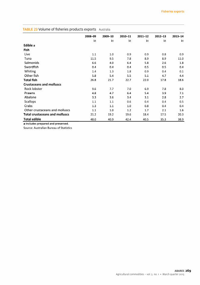
269ABARESAgricultural commodities – vol. 5 no. 1 • March quarter 2015
Fisheries exports
TABLE 23 Volume of fisheries products exports Australia
STATISTICS
23 Volume of fisheries products exports Australia23VolumeoffisheriesproductsexportsAustralia2008–09 2009–10 2010–11 2011–12 2012–13 2013–142008–09 2009–10 2010–11 2011–12 2012–13 2013–14
k k k k k kkt kt kt kt kt ktEdible aFishEdible aFishLi 1 1 1 0 0 9 0 9 0 8 0 9 Live 1.1 1.0 0.9 0.9 0.8 0.9 Tuna 11.5 9.5 7.8 8.9 8.9 11.0 Tuna 11.5 9.5 7.8 8.9 8.9 11.0Salmonids 6 6 4 0 6 4 5 8 2 6 1 8 Salmonids 6.6 4.0 6.4 5.8 2.6 1.8Swordfish 0 4 0 4 0 4 0 5 0 5 0 4 Swordfish 0.4 0.4 0.4 0.5 0.5 0.4Whi i Whiting 1.4 1.3 1.8 0.9 0.4 0.1g Other fish 5.8 5.4 5.5 5.1 4.7 4.4 Other fish 5.8 5.4 5.5 5.1 4.7 4.4Total fish 26 8 21 7 22 7 22 0 17 8 18 6Total fish 26.8 21.7 22.7 22.0 17.8 18.6C t d llCrustaceans and molluscs Rock lobster 9.6 7.7 7.0 6.9 7.8 8.0 Rock lobster 9.6 7.7 7.0 6.9 7.8 8.0Prawns 4.8 4.7 6.4 5.4 3.9 7.1 Prawns 4.8 4.7 6.4 5.4 3.9 7.1Abalone 3 3 3 6 3 4 3 1 2 8 2 7 Abalone 3.3 3.6 3.4 3.1 2.8 2.7S ll Scallops 1.1 1.1 0.6 0.4 0.4 0.5p Crabs 1.3 1.1 1.0 0.8 0.4 0.4 Crabs 1.3 1.1 1.0 0.8 0.4 0.4Other crustaceans and molluscs 1 1 1 0 1 2 1 7 2 1 1 6 Other crustaceans and molluscs 1.1 1.0 1.2 1.7 2.1 1.6Total crustaceans and molluscs 21 2 19 2 19 6 18 4 17 5 20 3Total crustaceans and molluscs 21.2 19.2 19.6 18.4 17.5 20.3Total edible 48.0 40.9 42.4 40.5 35.3 38.9Total edible 48.0 40.9 42.4 40.5 35.3 38.9a Includes prepared and preserveda Includes prepared and preserved.Source: Australian Bureau of StatisticsSource: Australian Bureau of Statistics

270 ABARESAgricultural commodities – vol. 5 no. 1 • March quarter 2015
Fisheries exports
TABLE 24 Value of fisheries products exports (fob) Australia
STATISTICS
2008–09 2009–10 2010–11 2011–12 2012–13 2013–14$m $m $m $m $m $m
Fish Live 46.5 40.4 33.4 32.0 30.7 34.2 Tuna 176.8 118.5 131.4 162.7 162.6 135.5 Salmonids 47.2 29.6 54.4 41.8 25.4 17.4 Swordfish 3.6 4.2 4.5 4.2 3.9 3.9 Whiting 3.4 3.4 5.0 2.5 1.4 0.2 Other fish 55.7 61.6 58.1 46.2 34.2 34.2Total fish 333.1 257.8 286.8 289.4 258.2 225.4
Rock lobster 461.6 399.7 369.3 386.7 447.3 590.3 Prawns 82.2 61.5 77.1 66.7 51.8 101.0 Abalone 208.2 216.4 212.0 197.3 186.0 170.0 Scallops 33.3 29.5 15.4 15.3 10.8 13.6 Crabs 16.4 13.8 13.4 11.0 8.2 5.5Other crustaceans and molluscs 9.7 8.5 16.3 34.4 40.2 32.5Total crustaceans and molluscs 811.4 729.3 703.6 711.3 744.2 912.9Total edible 1 144.5 987.1 990.3 1 000.7 1 002.3 1 138.3
Marine fats and oils 5.0 4.8 5.4 7.3 10.0 9.1 Fish meal 1.3 2.1 1.6 0.4 1.0 0.7 Pearls a 366.4 243.9 241.3 206.6 151.5 144.4 Ornamental fish 3.4 2.7 2.3 2.3 3.8 2.0 Other non‐edible 7.8 5.5 7.3 9.4 6.5 9.7Total non‐edible 384.0 259.0 257.9 226.1 172.8 165.9Total fisheries products 1 528.5 1 246.1 1 248.2 1 226.8 1 175.2 1 304.3
24Valueoffisheriesproductsexports(fob)Australia
Edible
Crustaceans and molluscs
Non‐edible
a Includes items temporarily exported and re‐imported.Source: Australian Bureau of Statistics

271ABARESAgricultural commodities – vol. 5 no. 1 • March quarter 2015
Fisheries imports
TABLE 25 Volume of fisheries products imports Australia2525 Volume of fisheries products imports Australia25VolumeoffisheriesproductsimportsAustralia2008–09 2009–10 2010–11 2011–12 2012–13 2013–142008–09 2009–10 2010–11 2011–12 2012–13 2013–14
kt kt kt kt kt ktkt kt kt kt kt ktEdible aFishEdible aFishTuna 38 0 39 9 45 6 40 8 46 9 50 1 Tuna 38.0 39.9 45.6 40.8 46.9 50.1 Salmonids 10.9 9.8 9.9 10.2 11.9 14.2Hake 5.7 5.4 6.7 5.3 6.1 4.5 Hake 5.7 5.4 6.7 5.3 6.1 4.5Swordfish 0 2 0 2 0 2 0 2 0 2 0 2 Swordfish 0.2 0.2 0.2 0.2 0.2 0.2T thfi h 0 1 0 1 0 1 0 1 0 2 0 2 Toothfish 0.1 0.1 0.1 0.1 0.2 0.2 Herrings 0.8 0.9 1.0 0.9 1.8 0.9 Herrings 0.8 0.9 1.0 0.9 1.8 0.9Shark 0.5 0.6 0.5 0.5 0.5 0.7 Shark 0.5 0.6 0.5 0.5 0.5 0.7Other fish 77 2 83 3 83 1 86 6 92 8 90 0 Other fish 77.2 83.3 83.1 86.6 92.8 90.0Total fish b 133.4 140.3 147.1 144.4 160.5 160.8Crustaceans and molluscsPrawns 26 7 34 5 32 6 37 5 34 8 38 7Crustaceans and molluscs Prawns 26.7 34.5 32.6 37.5 34.8 38.7L b t 0 5 0 7 0 9 0 9 0 8 1 0 Lobster 0.5 0.7 0.9 0.9 0.8 1.0 Crabs 1.0 1.2 1.4 1.5 1.5 2.1 Crabs 1.0 1.2 1.4 1.5 1.5 2.1Mussels 2.8 2.4 2.6 2.8 3.7 3.6 Mussels 2.8 2.4 2.6 2.8 3.7 3.6Scallops 2 2 2 8 2 6 3 0 3 1 3 5 Scallops 2.2 2.8 2.6 3.0 3.1 3.5S id d t 16 8 16 0 15 2 17 0 19 9 23 2 Squid and octopus 16.8 16.0 15.2 17.0 19.9 23.2q p Other crustaceans and molluscs 9.9 9.6 9.4 7.3 4.1 4.8 Other crustaceans and molluscs 9.9 9.6 9.4 7.3 4.1 4.8Total crustaceans and molluscs 59 9 67 2 64 7 69 8 67 9 76 7Total crustaceans and molluscs 59.9 67.2 64.7 69.8 67.9 76.7T t l dibl b 193 3 207 4 211 8 214 2 228 4 237 5Total edible abc 193.3 207.4 211.8 214.2 228.4 237.5a Includes prepared and preserved. b Excludes live tonnage. c Includes other fisheries products not classified into fish or p p p g pcrustaceans and molluscs.crustaceans and molluscs.Source: Australian Bureau of StatisticsSource: Australian Bureau of Statistics

272 ABARESAgricultural commodities – vol. 5 no. 1 • March quarter 2015
Fisheries imports
TABLE 26 Value of fisheries products imports Australia
STATISTICS
26 Value of fisheries products imports Australia26ValueoffisheriesproductsimportsAustralia2008–09 2009–10 2010–11 2011–12 2012–13 2013–142008–09 2009–10 2010–11 2011–12 2012–13 2013–14
$ $ $ $ $ $$m $m $m $m $m $mEdible aFishEdible aFishT 223 3 169 3 200 8 205 5 258 2 296 1 Tuna 223.3 169.3 200.8 205.5 258.2 296.1 Salmonids 100.0 85.8 84.4 91.8 118.8 167.5 Salmonids 100.0 85.8 84.4 91.8 118.8 167.5Hake 31 0 26 1 27 2 20 9 23 4 19 5 Hake 31.0 26.1 27.2 20.9 23.4 19.5Swordfish 1 5 1 8 1 5 1 2 1 7 1 4 Swordfish 1.5 1.8 1.5 1.2 1.7 1.4T hfi h Toothfish 1.0 1.3 1.4 1.3 2.2 3.0 Herrings 4.4 4.5 4.3 4.2 5.1 4.5 Herrings 4.4 4.5 4.3 4.2 5.1 4.5Shark 4 5 5 6 4 4 4 0 4 6 5 5 Shark 4.5 5.6 4.4 4.0 4.6 5.5Other fish 455 5 455 0 443 7 459 6 480 0 507 5 Other fish 455.5 455.0 443.7 459.6 480.0 507.5Total fish b 824.6 751.5 769.1 788.6 866.5 1 004.9Total fish bCrustaceans and molluscsPrawns 270 7 298 7 291 0 350 9 304 8 495 1Crustaceans and molluscs Prawns 270.7 298.7 291.0 350.9 304.8 495.1L b Lobster 9.8 11.8 15.0 16.0 15.3 22.4 Crabs 11.3 12.4 13.3 15.5 16.8 28.3 Crabs 11.3 12.4 13.3 15.5 16.8 28.3Mussels 12 0 9 3 10 2 11 7 17 1 19 1 Mussels 12.0 9.3 10.2 11.7 17.1 19.1Scallops 29 9 33 5 34 5 43 6 41 1 52 9 Scallops 29.9 33.5 34.5 43.6 41.1 52.9
d d Squid and octopus 54.3 62.0 74.3 90.4 97.7 114.5q p Other crustaceans and molluscs 70.1 66.5 65.3 57.0 40.7 44.0 Other crustaceans and molluscs 70.1 66.5 65.3 57.0 40.7 44.0Total crustaceans and molluscs 458 1 494 2 503 5 585 1 533 4 776 3Total crustaceans and molluscs 458.1 494.2 503.5 585.1 533.4 776.3T l dibl b 1 279 4 1 243 9 1 271 3 1 373 8 1 427 7 1 781 3Total edible abc 1 279.4 1 243.9 1 271.3 1 373.8 1 427.7 1 781.3Non‐ediblePearls d 320 6 170 8 166 9 138 2 105 4 102 1Non ediblePearls d 320.6 170.8 166.9 138.2 105.4 102.1Fish meal 41 9 51 9 46 7 34 2 43 3 43 2Fish meal 41.9 51.9 46.7 34.2 43.3 43.2
l fi hOrnamental fish 5.8 4.6 3.9 3.7 4.0 4.5Marine fats and oils 33.9 26.8 31.0 39.5 39.1 40.1Marine fats and oils 33.9 26.8 31.0 39.5 39.1 40.1Other marine products 24 9 14 9 9 9 17 1 29 0 30 4Other marine products 24.9 14.9 9.9 17.1 29.0 30.4Total non edible 427 1 269 0 258 4 232 8 220 7 220 3Total non‐edible 427.1 269.0 258.4 232.8 220.7 220.3Total fisheries products 1 706.5 1 512.9 1 529.7 1 606.6 1 648.4 2 001.6Total fisheries products 1 706.5 1 512.9 1 529.7 1 606.6 1 648.4 2 001.6a Includes prepared and preserved b Includes live value c Includes other fisheries products not classified into fish ora Includes prepared and preserved. b Includes live value. c Includes other fisheries products not classified into fish or
t d ll dM i l i tcrustaceans and molluscs. d Mainly re‐imports.Source: Australian Bureau of Statistics

273ABARESAgricultural commodities – vol. 5 no. 1 • March quarter 2015
Fisheries trade
TABLE 27 Value of Australian fisheries products trade, by selected countries Australia
STATISTICS
2008–09 2009–10 2010–11 2011–12 2012–13 2013–14$m $m $m $m $m $m
Hong Kong 570.1 530.0 425.9 479.1 317.0 208.9Vietnam 3.2 4.3 8.4 60.5 293.2 565.6Japan 302.5 215.5 225.9 254.6 236.0 192.1China 29.9 43.5 143.2 58.5 45.2 36.6Singapore 43.6 37.4 41.2 42.5 31.0 34.2United States 64.9 49.5 35.7 23.1 17.9 22.1Taiwan 53.8 32.5 29.6 17.5 9.8 13.7Thailand 7.3 9.0 16.0 18.1 9.3 8.0New Zealand 8.8 16.6 9.6 10.1 9.1 14.5Malaysia 12.7 9.2 12.9 7.7 7.8 9.9Indonesia 4.7 6.9 8.7 6.1 7.4 9.9
Hong Kong 201.0 137.8 145.1 96.6 54.3 74.6Japan 64.3 49.8 43.3 44.4 33.0 26.9United States 22.2 15.5 8.1 22.2 21.0 19.2
Thailand 367.9 322.1 340.2 362.1 399.8 417.0New Zealand 206.9 212.3 210.0 197.3 206.3 206.8China 151.7 173.0 185.6 231.5 196.5 341.5Vietnam 167.4 152.7 161.7 174.5 163.1 231.7Malaysia 65.2 63.0 71.2 73.2 81.0 97.9United States 49.4 37.3 39.9 45.1 52.2 56.0Indonesia 30.9 38.9 27.9 36.3 50.9 73.5Taiwan 32.9 36.7 39.5 38.9 48.1 44.5South Africa 36.0 35.8 33.1 32.2 36.2 50.5Denmark 23.4 29.6 28.2 31.3 35.1 31.6Norway 24.2 23.6 18.8 25.3 32.2 44.8Other 20.1 26.7 24.7 27.1 29.9 45.4
27ValueofAustralianfisheryproductstrade,byselectedcountriesAustrali
a Country details for non‐edible imports are not available.Source: Australian Bureau of Statistics
Exports
Imports a
Edible (including live)
Non‐edible
Edible (excluding live)

274 ABARESAgricultural commodities – vol. 5 no. 1 • March quarter 2015
Forest exports
TABLE 28 Volume of forest products exports Australia
STATISTICS
unit 2008–09 2009–10 2010–11 2011–12 2012–13 2013–14
Roundwood ’000 m3 986 1 377 1 638 1 806 1 516 2 363
Softwood roughsawn ’000 m3 283 322 265 198 207 268 Softwood dressed ’000 m3 18 13 13 13 3 5 Hardwood roughsawn ’000 m3 40 37 39 26 20 73 Hardwood dressed ’000 m3 14 16 30 15 7 25 Total ’000 m3 355 387 348 252 237 371Railway sleepers ’000 m3 9 9 8 8 8 17
Veneers ’000 m3 86 90 119 106 52 64 Plywood ’000 m3 53 24 7 18 36 36 Particleboard ’000 m3 17 9 5 4 2 6 Hardboard b ’000 m3 2 1 2 2 2 3 Medium‐density fibreboard ’000 m3 181 130 115 79 52 172 Softboard and other fibreboards ’000 m3 8 2 5 5 1 1 Total ’000 m3 345 256 253 214 146 280Paper and paperboard Newsprint kt 2 6 19 30 72 85 Printing and writing kt 112 146 84 132 139 153 Household and sanitary kt 38 31 39 26 12 20 Packaging and industrial kt 617 708 887 933 906 950 Total kt 769 890 1 029 1 121 1 127 1 207Recovered paper kt 1 216 1 444 1 323 1 403 1 506 1 449Pulp kt 22 18 31 1 0 0Woodchips cd kt 5 255 4 818 5 064 4 150 3 806 4 776
Quantity
Sawnwood a
Wood‐based panels
28VolumeofforestryproductexportsAustralia
a Excludes railway sleepers. b Uncoated hardboard confidential from January 2007. c Includes particles. d Bone dry tonnes.Note: Components may not add to totals due to rounding. Zero is used to denote nil or less than 500 tonnes.Sources: ABARES; Australian Bureau of Statistics; Engineered Wood Products Association of Australasia

275ABARESAgricultural commodities – vol. 5 no. 1 • March quarter 2015
Forest exports
TABLE 29 Value of forest products exports (fob) Australia
STATISTICS
2008–09 2009–10 2010–11 2011–12 2012–13 2013–14$m $m $m $m $m $m
Roundwood 101 138 198 175 155 292
Softwood roughsawn 70 76 67 55 61 75 Softwoods dressed 9 7 5 3 2 3 Hardwood roughsawn 37 33 34 23 20 22 Hardwood dressed 9 10 10 7 6 7 Total 125 125 115 88 90 108Railway sleepers 4 2 3 3 3 3Miscellaneous forest products a 54 61 66 59 54 63
Veneers 36 44 52 51 24 29 Plywood 4 3 2 2 4 3 Particleboard 7 3 2 1 1 1 Hardboard b 1 1 2 2 2 2 Medium‐density fibreboard c 52 45 39 26 19 26 Softboard and other fibreboards 1 1 1 1 0 0 Total 101 97 98 83 51 62
Newsprint 2 6 13 15 36 59 Printing and writing 128 143 88 120 117 139 Household and sanitary 111 97 94 64 33 49 Packaging and industrial 364 404 552 518 526 605 Total 606 649 747 717 712 853Paper manufactures d 106 102 112 134 132 132Recovered paper 235 228 240 240 230 241Pulp 18 13 11 1 0 0Woodchips 997 856 884 729 611 768Total 2 346 2 271 2 475 2 229 2 037 2 520a Includes such items as wooden doors, mouldings, packing cases, parquetry flooring, builders carpentry, cork, gums, resins, eucalyptus oils and other miscellaneous wood articles. Excludes wooden furniture. b Uncoated hardboard confidential from January 2007. c Some categories of medium‐density fibreboard are confidential. d Includes other paper articles that have had some further processing.Note: Components may not add to totals due to rounding. Zero is used to denote nil or less than $0.5 million.Sources: ABARES; Australian Bureau of Statistics; Engineered Wood Products Association of Australasia
Value
Sawnwood
Paper and paperboard
Wood‐based panels
29Valueofforestryproductsexports(fob)Australia
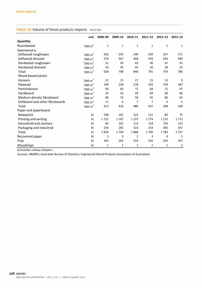
276 ABARESAgricultural commodities – vol. 5 no. 1 • March quarter 2015
Forest imports
TABLE 30 Volume of forest products imports Australia
unit 2008–09 2009–10 2010–11 2011–12 2012–13 2013–14
Roundwood ’000 m3 1 1 1 1 1 1Sawnwood a Softwood roughsawn ’000 m3 256 293 290 239 247 271 Softwood dressed ’000 m3 279 367 468 470 443 449 Hardwood roughsawn ’000 m3 51 43 43 46 41 41 Hardwood dressed ’000 m3 43 45 45 36 28 25 Total ’000 m3 628 748 846 791 759 786
Veneers ’000 m3 21 15 17 15 13 9 Plywood ’000 m3 199 228 278 293 278 287 Particleboard ’000 m3 69 64 72 68 72 97 Hardboard ’000 m3 24 33 49 69 60 86 Medium‐density fibreboard ’000 m3 88 70 58 95 80 65 Softboard and other fibreboards ’000 m3 11 6 7 7 6 5 Total ’000 m3 412 416 480 547 508 549
Newsprint kt 198 191 222 121 85 75 Printing and writing kt 1 122 1 167 1 237 1 174 1 155 1 172 Household and sanitary kt 82 101 114 118 159 123 Packaging and industrial kt 254 285 314 333 385 357 Total kt 1 656 1 744 1 886 1 746 1 783 1 727Recovered paper kt 3 3 2 3 4 5Pulp kt 345 265 233 256 263 297Woodchips kt 1 1 1 1 1 2
30VolumeofforestryproductimportsAustralia
Wood‐based panels
Paper and paperboard
Quantity
a Excludes railway sleepers.Sources: ABARES; Australian Bureau of Statistics; Engineered Wood Products Association of Australasia

277ABARESAgricultural commodities – vol. 5 no. 1 • March quarter 2015
Forest imports
TABLE 31 Value of forest products imports Australia
STATISTICS
2008–09 2009–10 2010–11 2011–12 2012–13 2013–14$m $m $m $m $m $m
Roundwood 1 0 1 1 1 1
Softwood roughsawn 134 140 135 105 100 111 Softwood dressed 168 200 248 248 246 281 Hardwood roughsawn 49 39 40 44 41 46 Hardwood dressed 55 50 50 51 35 31 Total 405 429 473 448 423 468Miscellaneous forest products a 675 630 707 756 769 946
Veneers 28 22 21 21 19 15 Plywood 145 138 170 183 184 210 Particleboard 27 20 21 26 27 35 Hardboard 26 30 40 54 48 72 Medium‐density fibreboard 41 37 34 36 32 35 Softboard and other fibreboards 4 3 3 3 2 3 Total 271 250 289 323 311 370
Newsprint 173 158 176 91 58 49 Printing and writing 1 468 1 355 1 347 1 217 1 151 1 194 Household and sanitary 154 164 185 187 244 208 Packaging and industrial 481 499 515 543 590 654 Total 2 276 2 175 2 223 2 037 2 043 2 105Paper manufactures b 590 563 557 486 446 537Recovered paper 1 1 0 1 1 2Pulp 263 178 180 164 154 203Woodchips 2 1 2 2 3 3Total 4 484 4 227 4 431 4 217 4 151 4 636
Value
Sawnwood
Wood‐based panels
Paper and paperboard
31ValueofforestryproductsimportsAustralia
a Includes such items as wooden doors, mouldings, packing cases, parquetry flooring, builders carpentry, cork, gums, resins, eucalyptus oils and other miscellaneous wood articles. Excludes wooden furniture. b Includes other paper articles that have had some further processing.Note: Components may not add to totals due to rounding. Zero used to denote nil or less than $0.5 million.Sources: ABARES; Australian Bureau of Statistics; Engineered Wood Products Association of Australasia

278 ABARESAgricultural commodities – vol. 5 no. 1 • March quarter 2015
TABLE 32 Value of Australian forest products trade, by selected countries a
STATISTICS
32 Value of Australian forestry products trade, by selected countries a32ValueofAustralianforestryproductstrade,byselectedcountriesa2008–09 2009–10 2010–11 2011–12 2012–13 2013–142008–09 2009–10 2010–11 2011–12 2012–13 2013–14
$ $ $ $ $ $$m $m $m $m $m $mExports bChina 390 394 544 534 474 naExports bChina 390 394 544 534 474 naH K 51 69 42 39 16Hong Kong 51 69 42 39 16 naJapan 860 774 745 579 394 naJapan 860 5 5 9 39 aKorea, Rep. of 103 48 40 40 33 naKorea, Rep. of 103 48 40 40 33 naMalaysia 79 324 1 553 112 113 naMalaysia 79 324 1 553 112 113 naN Z l d 324 320 315 306 268New Zealand 324 320 315 306 268 naTaiwan 78 88 79 68 68 naTaiwan 78 88 79 68 68 naImportsChi 617 635 690 800 913ImportsChina 617 635 690 800 913 naFinland 274 172 143 120 205 naFinlandGermany 169 179 183 148 135 naGermany 169 179 183 148 135 naIndonesia 375 355 332 342 313 naIndonesia 375 355 332 342 313 naM l i 216 218 228 236 227Malaysia 216 218 228 236 227 nayNew Zealand 747 707 715 634 557 naNew Zealand 747 707 715 634 557 naUnited States 321 315 285 298 304 naUnited States 321 315 285 298 304 naa Value of wood products trade to selected countries cannot be reported for 2013 14 due to confidentiality restrictions fora Value of wood products trade to selected countries cannot be reported for 2013–14 due to confidentiality restrictions for
d hi d d i b l f d d l d i l d dwoodchip exports and some paper product imports. b Value of wood products exports to selected countries may exclude data where confidentiality restrictions apply. na Not available.where confidentiality restrictions apply. na Not available.Sources: ABARES; Australian Bureau of StatisticsSources: ABARES; Australian Bureau of Statistics
Forestry trade

ABARESAgricultural commodities – vol. 5 no. 1 • March quarter 2015
ABARES reports released since Agricultural commodities (vol. 4 no. 4 December quarter 2014)The selection provides an overview of the range of interests ABARES covers.
Full reports can be downloaded from agriculture.gov.au/abares/publications. For more information contact [email protected].
Research reports
Australian dairy: financial performance of dairy farms, 2011–12 to 2013–14 Publication date: 16 December 2014Author: Dale Ashton
This report covers trends in farm financial performance of Australian dairy farms up to and including 2013–14. It includes analysis of changes in farm financial performance, debt and equity. Detailed analysis by farm size highlights differences in farm physical and financial performance across the industry.
Other reports
Status of key Australian fish stocks reports 2014 Publication date: 10 December 2014
This report provides scientifically based national assessments of the status of key wild-capture fish stocks. Together, the 68 key species (or species complexes) assessed in the report represent over 90 per cent of the value and 85 per cent of the volume from Australian fisheries.
279
Report extracts

ABARESAgricultural commodities – vol. 5 no. 1 • March quarter 2015
Building on the 2012 inaugural edition, this report assesses 19 additional species, four of which are caught in Commonwealth fisheries. The states and the Northern Territory nominated these species as either iconic and likely to be seen in retail outlets or as historically overfished.
The report was produced in collaboration with universities and Commonwealth and state government agencies.
Agricultural commodity statistics 2014 Publication date: 16 December 2014
This annual compendium of historical statistics covers the agriculture, fisheries, food and forestry sectors. It provides a set of comprehensive statistical tables on Australian and world prices, production, consumption, and stocks and trade for 19 rural commodities.
Commodities covered include grains and oilseeds, livestock, livestock products, food, wool, horticulture, forestry products and fisheries products. Also included are statistics on agricultural water use and macroeconomic indicators such as economic growth, employment, balance of trade, exchange rates and interest rates.
Regional farm debt: northern Queensland gulf, south west Queensland and north west New South Wales Publication date: 4 December 2014
ABARES prepared this report in response to a commitment made at the Agricultural Finance Forum in Canberra on 23 September 2014. The report, developed in consultation with the Australian Bankers’ Association (ABA) and the National Farmers’ Federation, provides a snapshot of the current level of farm debt in the northern Queensland gulf region, south west Queensland and north western New South Wales. Data were drawn from ABARES, the Australian Bankers’ Association, the Australian Bureau of Statistics, Australian Prudential Regulation Authority and the Queensland Gulf Cattlemen’s Association.
Australian crop report Publication date: 10 February 2014
This quarterly report provides a consistent and regular assessment of crop prospects for major field crops, forecasts of area, yield and production and a state-by-state summary of seasonal conditions.
Weekly Australian climate, water and agricultural update Publication date: Every Thursday
This weekly report contains information previously published in the Australian climate and agricultural monthly update. The combined weekly and monthly updates provide subscribers with improved access to up-to-date climate, water and commodity information in a single report.
Report extracts
280

ABARESAgricultural commodities – vol. 5 no. 1 • March quarter 2015
281
Executive Director Karen Schneider [email protected] (02) 6272 4636 Agricultural Commodities and Trade Assistant Secretary and Chief Commodity Analyst Jammie Penm [email protected] (02) 6272 2030Agricultural Trade Caroline Gunning-Trant [email protected] (02) 6272 2123Agricultural Commodities Peter Collins [email protected] (02) 6272 2017Outlook Engagement Anna Carr [email protected] (02) 6272 2287Agricultural Risks Management Matthew Miller [email protected] (02) 6272 3527
Farm Analysis and BiosecurityAssistant Secretary Peter Gooday [email protected] (02) 6272 2138Productivity Alistair Davidson [email protected] (02) 6272 2487Infrastructure and Water Tim Goesch [email protected] (02) 6272 2009Farm Survey and Analysis Milly Lubulwa [email protected] (02) 6272 2069Biosecurity Emily Gray [email protected] (02) 6272 2063Invasives and Social Sciences Bertie Hennecke [email protected] (02) 6272 4263
Fisheries, Forestry and LandAssistant Secretary Ilona Stobutzki [email protected] (02) 6272 4277Domestic Fisheries and Marine Peter Ward [email protected] (02) 6272 2015International Fisheries and Data James Larcombe [email protected] (02) 6272 3388Fisheries Economics Robert Curtotti [email protected] (02) 6272 2014Quantitative Sciences Belinda Barnes [email protected] (02) 6272 5374Forest Sciences Steve Read [email protected] (02) 6272 5582Forest Economics Beau Hug [email protected] (02) 6272 3929Data and Land John Sims [email protected] (02) 6272 5732
Editing, Production, Online and Design John Wilson [email protected] (02) 6272 3811Library Resources Karen Kidd [email protected] (02) 6272 4548Media [email protected] (02) 6272 3232Publication inquiries [email protected] (02) 6272 2010
ABARES contacts
Agricultural commodities March quarter 2015 was designed and produced by the Department of Agriculture and the Agricultural Commodities team of ABARES. Editors: Jane Wiles and Emma Rossiter

agriculture.gov.au/abares
Australian Bureau of Agricultural and Resource Economics and Sciences (ABARES)
Postal address GPO Box 858 Canberra ACT 2601
Switchboard +61 2 6272 3933
Facsimile +61 2 6272 2001
Email [email protected]
Web agriculture.gov.au/abares
Also in this series• Agricultural commodities, December 2013• Agricultural commodities, March 2014• Agricultural commodities, June 2014• Agricultural commodities, September 2014• Agricultural commodities, December 2014
The ‘Biosphere’ Graphic ElementThe biosphere is a key part of the department’s visual identity. Individual biospheres are used to visually describe the diverse nature of the work we do as a department, in Australia and internationally.
ABA
1836
_011
5


![ION Late Payments September Quarter AU [NewTemplate] · 2019. 11. 12. · Late payments by sector Late Payments by Sector - September Quarter 2019 There were four sectors that bucked](https://img.pdfslide.net/doc/110x75/60fc711994bf916c215c851d/ion-late-payments-september-quarter-au-newtemplate-2019-11-12-late-payments.jpg)