Agricultural Diversification and its Impact on Farm …ageconsearch.umn.edu/record/265244/files/7-B-Sen.pdfRelating it to farm level situation, the primary survey in Banka and Bhagalpur

Agricultural Economics Research ReviewVol. 30 (Conference Number) 2017 pp 77-88DOI: 10.5958/0974-0279.2017.00023.4

Agricultural Diversification and its Impact on Farm Income:A Case Study of Bihar

Biswajit Sen*, P. Venkatesh, Girish K. Jha, D.R. Singh and Suresh A.Division of Agricultural Economics, ICAR-Indian Agricultural Research Institute, New Delhi-110 012

Abstract

This paper has assessed the diversification scenario of agriculture at the national level and its reflectionat farm level situation alongside. It has been observed that concentration ratio (CR4) for four majoragricultural sub-sectors has declined from 73.6 per cent to 69.6 per cent for the study period, 1999-00 to2013-14. It clearly indicates a shift in Indian agriculture from cereals-based production pattern to otherhigh-value based production pattern. However, Simpson Index for Diversification (SID) indicates thatthe average national SID for all agricultural enterprises is 0.83 which spans from 0.60 for Punjab to 0.89for Karnataka. Relating it to farm level situation, the primary survey in Banka and Bhagalpur districts ofBihar has been carried out in 2016-17 to find out the impact of agricultural diversification on farmincome with two-stage least square technique (2SLS). Empirical analysis has suggested that diversificationof farm by adopting ancillary, horticulture and other HVE like mushroom, etc. will increase farm income.

Key words: Agricultural diversification, Simpson index of diversification, two-stage least square, highvalue enterprise, farm income

JEL Classification: Q12, Q18, Q19

IntroductionIn India, agriculture is a major sector that plays a

crucial role in the development of agrarian economies.However, agriculture sector in India has witnesseddrastic changes after introduction of moderntechnology during green revolution in mid-1960s.Green revolution provided boost to the economy byachieving significant uptrend in cereals-based croppingpattern than less profitable existing crop-mix. As aresult, now 50 per cent of gross cropped area comesunder high productive major cereal crops, leading tocropping pattern very much skewed towards cereal-based farming which results in low degree ofdiversification. Although this situation is changing asthe area under so-called commercial crops (non-food

crops) has doubled since the 1960s and now equalshalf of the area under food crops (Vyas, 1996), the paceis however meagre. Experiences from differentdeveloping countries corroborate the key role ofdiversification in agricultural development andsustainability (Petit and Barghouti, 1992; Pingali andRosegrant, 1995; Birthal et al., 2005; 2015; Singh etal., 2006), but many researchers are sceptical aboutthis view (Pretty, 1994; Hardaker, 1997) and believethat high diversification is stratagem of subsistenceoriented farming systems (Morris and Winter, 1999).Therefore, in this context it is important to understandthe effect of diversification on production andproductivity as they may or may not be alwayspositively correlated (Cochrane et al., 1994).

In India, the studies on agricultural diversificationare mainly region-based due to diverse agriculturalsituations of the country. Most of these studies have

*Author for correspondenceEmail: [email protected]

78 Agricultural Economics Research Review Vol. 30 (Conference Number) 2017

concentrated on crop diversification by constructingSimpson Index of Diversification (SID) which werearea based approach neglects importance of some high-value enterprise like spices and condiments, viz. blackpepper, cardamom, etc. where area of cultivation ismeagre but value of output generated is considerable.The area-based approach also does not includelivestock and ancillary enterprises where area underenterprise is not important and it leads to partialconsideration of diversification situation neglecting thelivestock sub-sector. The established analysis oneconomics of agricultural diversification and farmincome also falls short in its coverage andperceptiveness. So, if the task is to predict the speed ofrestructuring of an economy and its industries that isbeing affected by backward linkages like agriculture,clear understanding of agricultural diversification isobligatory. In this context, this study analysedagricultural diversification in a holistic view with widercoverage of various activities in agriculture and alliedsector by following value of output approach from eachenterprise and subsector of agriculture and allied sector.The study has also analysed the effect of diversificationon farm income for selected districts of Bihar.

At present, the development of strategies foraugmenting the income of farmers, especially smalland marginal farmers, is the major challenge. So, Bihar,a state with more than ninety five percent of marginaland small farmers is selected purposively for a casestudy.

Data and MethodologyThe data used for analysing diversification across

different states of India were taken from the Ministryof Statistics and Programme Implementation (MoSPI),Government of India, for the time period 1999-00 to2013-14. The data series provide statistics on value ofoutput for all major crops and allied agriculturalactivities with base years 1999-00, 2004-05 and 2011-12. All values were further converted to 2011-12 baseyear by adjusting with agricultural GDP data series of2011-2 base year. The data on value of output ofagricultural and allied enterprises enabled us to estimatethe level of diversification with Simpson Index ofDiversification (SID).

…(1)

where,Value of output for ith crop

Pi = –––––––––––––––––––––––––––––––––––––––––––––––Total value of output from all agriculture and allied sectors

To assess the farm level situation, primary surveywas conducted in Bihar during 2016-17. The primarydata were collected form 120 farms in two districts(60 farms from each district) of Bihar. For study Bankaand Katoria blocks of Banka district and Sabour andKharik blocks of Bhagalpur district were selected.Multistage stratified random sampling was adopted forselecting high and low agricultural diversified districts.From each district two blocks, from each block, avillage cluster, within a village cluster, farms wereselected. The rationale behind classifying all districtsinto two strata was to capture all socio-economic andagronomic situations and conditions in two differentparent population in terms of diversification.

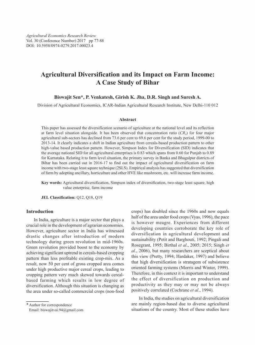
From district level cross-sectional primary data,SID was calculated to examine farm level picture ofagricultural diversification as micro-unit. Alongside,the effect of level and direction of diversification onfarm income was also assessed for the selected farmsusing econometric model [Equations (2)-(3)]. However,the variable, level of diversification (denoted by MSIDor modified SID) does not only affect farm income,but may also be affected by farm income alongside(Figure 1), resulting endogeneity bias due to presenceof bi-directional cause and effect relationship betweenendogenous variables which make the estimates ofparameter erroneous (Bravo-Ureta et al., 2006;Gavian and Fafchamps, 1996; Feder et al., 1985). Toaddress this problem and eliminate the probableendogeneity bias that may arise in this type ofanalysis, two-stage least square (2SLS) technique wasemployed.

The farm income model was constructed assumingendogeneity relation prevailing between farm incomeand level of diversification following the methodologyin literature, viz. Bravo-Ureta et al. (2006), Weiss andBriglauer (2000), IFPRI (2003).

Empirical Econometric Model

Variable Selection: The exogenous variablesincorporated in the empirical model were selectedfollowing existing literature on agriculturaldiversification (Kumar and Gupta, 2015; Birthal et al.,

Sen et al. : Agricultural Diversification and its Impact on Farm Income 79

Figure 1. Expected relationship between farm income, level of diversificationand other explanatory variables

2007; Singh et al., 2006) and on relationship betweenfarm income and agricultural diversification (Birthalet al., 2015; Bravo-Ureta et al., 2006). Table 1 portraysthe description of variables included in the empiricalmodel.

The Econometric Model

Farm Income = f (Diversification, Farm size, Irrigation, Wealth, Education, No. of livestock, etc.)

…(2)

Diversification = f (Farm Income, Farm size, Irrigation, Wealth, Education, No. of livestock, etc.)

…(3)

where, Y is the farm income, MSID is the modifiedSimpson Index as a measure of diversification ofagricultural activities included and Xi and Xj representall the exogenous variables included in the system ofequations.

Results and Discussions

Spatio Temporal Trend and AgriculturalDiversification Status across the Country

The skewed production pattern of the countrytowards cereals was the main driving force ofagriculture till the past few decades which is visibleby high share of value of output of cereals in total valueof output of all agricultural enterprises (Table 2).

It can be observed that Concentration Ratio (CR4)of highest four agricultural sub-sectors constitutesnearly 70 per cent of the total value of output fromagricultural crops. It clearly indicates that Indianagriculture has low level of diversification at the overalllevel. Despite having higher prices than cereals, pulsesand oilseeds had a very low share in total value ofagricultural output and even recorded a negative growthrate. Though was having a declining trend leadingtowards diversification for the period 1999-00 to 2013-14, it has very low magnitude. It can be also seen thatonly six to seven sub-sectors had a share of more than5 per cent in total value of output from agriculture in


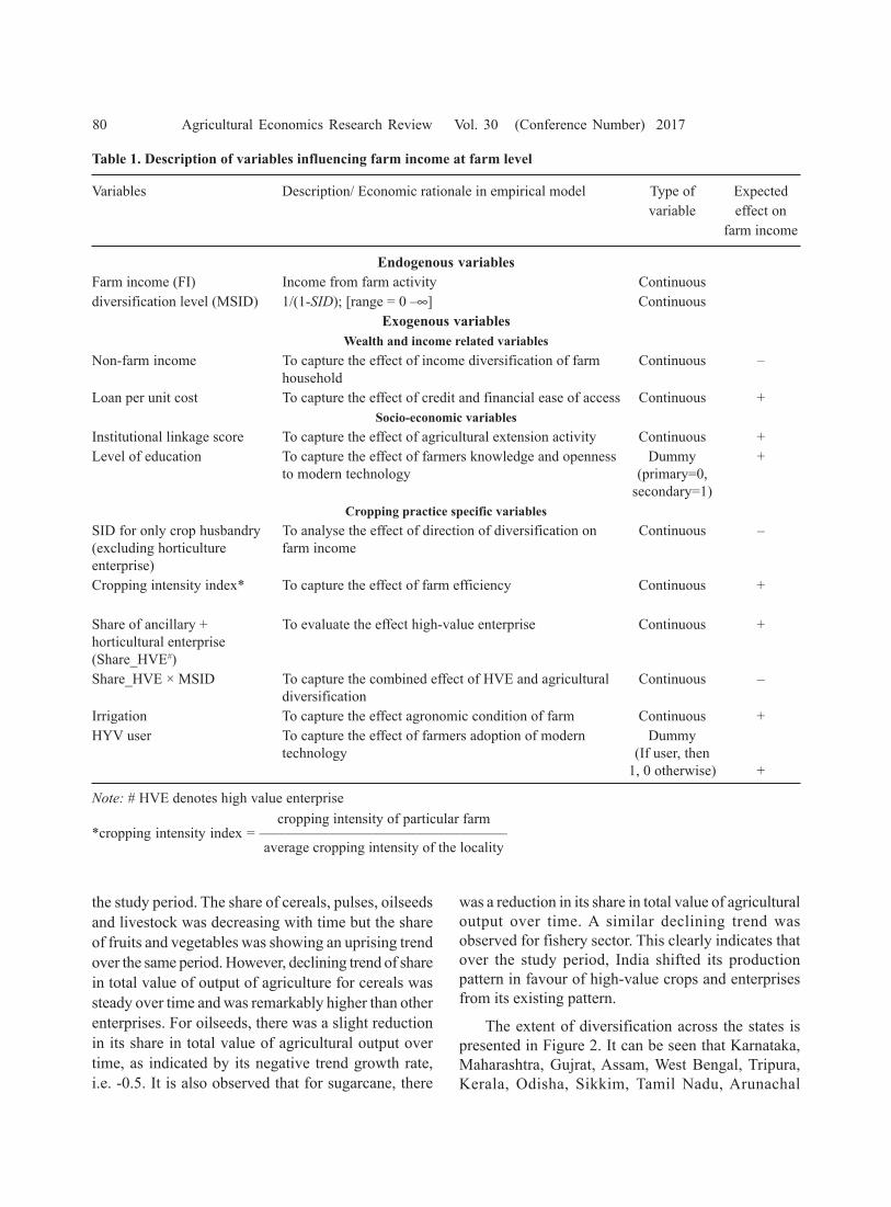
Table 1. Description of variables influencing farm income at farm level

Variables Description/ Economic rationale in empirical model Type of Expectedvariable effect on

farm income

Endogenous variablesFarm income (FI) Income from farm activity Continuousdiversification level (MSID) 1/(1-SID); [range = 0 –∞] Continuous

Exogenous variablesWealth and income related variables

Non-farm income To capture the effect of income diversification of farm Continuous –household

Loan per unit cost To capture the effect of credit and financial ease of access Continuous +Socio-economic variables

Institutional linkage score To capture the effect of agricultural extension activity Continuous +Level of education To capture the effect of farmers knowledge and openness Dummy +

to modern technology (primary=0,secondary=1)

Cropping practice specific variablesSID for only crop husbandry To analyse the effect of direction of diversification on Continuous –(excluding horticulture farm incomeenterprise)Cropping intensity index* To capture the effect of farm efficiency Continuous +

Share of ancillary + To evaluate the effect high-value enterprise Continuous +horticultural enterprise(Share_HVE#)Share_HVE × MSID To capture the combined effect of HVE and agricultural Continuous –

diversificationIrrigation To capture the effect agronomic condition of farm Continuous +HYV user To capture the effect of farmers adoption of modern Dummy

technology (If user, then1, 0 otherwise) +

Note: # HVE denotes high value enterprisecropping intensity of particular farm

*cropping intensity index = ––––––––––––––––––––––––––––––––––average cropping intensity of the locality

the study period. The share of cereals, pulses, oilseedsand livestock was decreasing with time but the shareof fruits and vegetables was showing an uprising trendover the same period. However, declining trend of sharein total value of output of agriculture for cereals wassteady over time and was remarkably higher than otherenterprises. For oilseeds, there was a slight reductionin its share in total value of agricultural output overtime, as indicated by its negative trend growth rate,i.e. -0.5. It is also observed that for sugarcane, there

was a reduction in its share in total value of agriculturaloutput over time. A similar declining trend wasobserved for fishery sector. This clearly indicates thatover the study period, India shifted its productionpattern in favour of high-value crops and enterprisesfrom its existing pattern.

The extent of diversification across the states ispresented in Figure 2. It can be seen that Karnataka,Maharashtra, Gujrat, Assam, West Bengal, Tripura,Kerala, Odisha, Sikkim, Tamil Nadu, Arunachal


Table 2. Sectorial share and trend in value of agricultural production in India: 1999-00 to 2013-14 (in per cent)

Year Cereals Oilseeds Pulses Livestock Fishery Fruits Vegetables Sugarcane Fibre & Spices and CR4

cash crops condiments

1999-00 27.5 7.19 3.44 28.5 5.01 8.55 8.95 3.93 4.66 2.19 73.62000-01 26.4 6.77 3.00 30.1 5.38 8.64 9.06 4.04 4.25 2.26 74.32001-02 26.6 7.06 3.36 29.5 5.27 8.70 9.14 3.78 4.27 2.25 74.02002-03 23.7 5.85 3.09 32.8 5.96 8.86 9.33 3.93 4.21 2.23 74.72003-04 25.0 8.06 3.53 29.8 5.46 8.75 9.23 2.90 4.84 2.32 72.92004-05 23.5 7.76 3.41 30.8 5.27 8.82 9.44 2.93 5.26 2.67 72.72005-06 22.9 8.36 3.27 30.1 5.26 8.79 9.61 3.62 5.39 2.62 71.52006-07 23.0 7.49 3.24 29.9 5.28 8.94 9.38 4.69 5.47 2.52 71.32007-08 22.9 7.79 3.26 29.3 5.27 8.91 9.46 4.37 5.96 2.63 70.72008-09 23.4 7.04 3.19 31.2 5.44 9.35 9.31 2.86 5.54 2.62 73.32009-10 21.4 6.77 3.12 31.9 5.51 9.71 10.0 3.27 5.37 2.80 73.12010-11 21.3 7.76 3.39 30.7 5.29 8.93 10.2 3.68 5.73 2.87 71.32011-12 19.6 6.24 3.05 31.9 4.68 9.59 10.2 3.52 8.28 2.71 69.52012-13 19.1 6.03 3.19 32.3 4.86 9.72 10.4 3.40 8.21 2.65 69.42013-14 18.8 5.87 3.22 32.2 5.00 9.74 10.4 3.11 8.72 2.75 69.6

Note: CR4 denotes Concentration ratio

Figure 2. State-wise average diversification level (1999-00 to 2013-14) for the overall agriculture (SID)


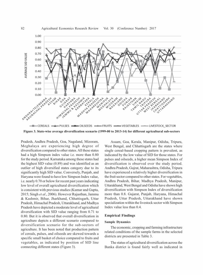
Pradesh, Andhra Pradesh, Goa, Nagaland, Mizoram,Meghalaya are experiencing high degree ofdiversification compared to other states. All these stateshad a high Simpson index value i.e. more than 0.80for the study period. Karnataka among these states hadthe highest SID value (0.89) and was identified as anoutlier of high diversified states category due to itssignificantly high SID value. Conversely, Punjab, andHaryana were found to have low Simpson Index value,i.e. nearly 0.70 or below for recent past years indicatinglow level of overall agricultural diversification whichis consistent with previous studies (Kumar and Gupta,2015; Singh et al., 2006). However Rajasthan, Jammu& Kashmir, Bihar, Jharkhand, Chhattisgarh, UttarPradesh, Himachal Pradesh, Uttarakhand, and MadhyaPradesh have depicted a moderate level of agriculturaldiversification with SID value ranging from 0.71 to0.80. But it is observed that overall diversification inagriculture depicts a different scenario compared todiversification scenario for the sub-sectors ofagriculture. It has been noted that production patternof cereals, pulses, and oilseeds are skewed towards aspecific small basket of choice compared to fruits andvegetables, as indicated by position of SID lineconnecting different states (Figure 3).

Assam, Goa, Kerala, Manipur, Odisha, Tripura,West Bengal, and Chhattisgarh are the states wheresingle cereal-based cropping pattern is prevalent, asindicated by the low value of SID for those states. Forpulses and oilseeds, a higher mean Simpson Index ofdiversification is observed over the study period.Andhra Pradesh, Gujrat, Maharashtra, Odisha, Tripurahave experienced a relatively higher diversification inthe fruit sector compared to other states. For vegetables,Andhra Pradesh, Bihar, Madhya Pradesh, Manipur,Uttarakhand, West Bengal and Odisha have shown highdiversification with Simpson Index of diversificationmore than 0.8. Gujarat, Punjab, Haryana, HimachalPradesh, Uttar Pradesh, Uttarakhand have shownspecialization within the livestock sector with SimpsonIndex value less than 0.4.

Empirical Findings

Sample Dynamics

The economic, cropping and farming infrastructurerelated conditions of the sample farms in the selecteddistricts are presented in Table 3.

The status of agricultural diversification across theBanka district is found fairly well as indicated in

Figure 3. State-wise average diversification scenario (1999-00 to 2013-14) for different agricultural sub-sectors


Table 3 which may be the result of occupation of highercultivated area per farm (0.81 ha compared to 0.4 hain Bhagalpur). However, as the districts fall in the sameagro-climatic sub-region, the variety of crops cultivatedin both the districts does not differ significantly butcropping pattern of farms are considerably different asindicated by their SID score. The per family income isalso higher for Banka than Bhagalpur which may bethe result of higher cropping land occupancy, highernumber of cattle per farm and higher cropping intensityin Banka district. The other parameter of sampleselection, i.e. average number of crops cultivated, isnearly similar for both the districts but allocation ofarea and share of each crop in total revenue of farmdiffers considerably, as implied by their SID score.Infrastructure facility does not diverge considerablyacross these two districts though Banka district has aslight edge over Bhagalpur in more developedinstitutional linkages.

Rationale for Agricultural Diversification

Diversification in agriculture commonly meansgrowing different crops instead of concentrating undera single crop. However, Pingali and Rosengrant (1995)defined diversification as “change in product (orenterprise) choice and input use decisions based onmarket forces and the principles of profitmaximization”. Conversely, Joshi et al. (2004) have

defined “agricultural diversification as movement ofproduction-portfolio from a low-value commodity mix(crop and livestock) to high-value commodity-mix(crops and livestock)” making a shift from traditionaldefinition. However, to encompass all the agriculturaland allied sector, diversification should be consideredas a strategy of changing crop or enterprise-mix withmore equivalent distributive share for each sector. Butthe rationale to select agricultural diversification as astrategy connects different logic viz. risk minimization,sustainability or high production depending on theintention of the farmer. The economic objective ofdifferent kinds of diversification has been presentedin Table 4.

Impact of Agricultural Diversification on FarmIncome

The estimates of parameters used in the empiricalmodel [Equations (2)-(3)] are presented in Table 5. Dueto possibility of presence of endogeneity bias in thesample, Durbin-Wu-Hausman test was employed toconfirm it. The test revealed the presence ofcontemporaneous correlation between the proposedendogenous variables and the error term in the farmincome equation at 10 per cent level of significanceand corroborated the assumption of endogeneity biasindicating preference of 2SLS over ordinary leastsquare model.

Table 3. Summary statistics for sample farms in selected districts of Bihar

Variable Banka BhagalpurMean Standard deviation Mean Standard deviation

Cropping schemeSimpson index of diversification 0.79 0.137 0.4 0.177Average farm size (ha) 0.81 1.479 0.59 1.0869Cropping intensity (%) 153.9 37.941 146.98 42.094Average No. of crops cultivated 2.9 1.203 2.866 1.255Share of ancillary & horticultural enterprise (%) 46.6 0.281 47.8 0.309

Economic schemeAverage No. of cattle per farm household 0.783 1.823 0.6 1.06Farm income per family (`) 58776 19548 46204 27686Cost A1 per farm per hectare 65759 67521 71698 54755

Infrastructure facilityFamily labour per farm 2.479 1.228 2.5 1Market distance (km) 4.24 2.661 4.56 2.131Institutional linkage score 1.566 0.302 1.1 0.62


Table 4. Economic intent for different types of diversification

Concept of Definition/ Strategy Economicdiversification objective

Horizontal diversification Farmer producer adds more crops to existing crop-mix in cropping Home consumption/pattern Risk reduction

Vertical diversification Farmer producer engages different value-added activities within its Incomeown farm augmentation

Spatial diversification Growing different crop-mix in a larger area To capture benefit ofintegrated farmingapproach

Temporal diversification Diversifying existing crop-mix for a particular farm, over time Sustainability ofcropping system

Structural diversification Makes crops within field more structurally diverse Risk reduction (Pest(Hossain et al., 2001) attack)

Genetic diversification Growing mixed variety of species in monoculture (Zhu et al., 2001) Risk reduction(Disease attack)

Crop rotation Rotating fixed number of crops in same field over time Enhancement of(Krupinsky et al., 2002; Smith et al., 2008) total production/

Risk reductionPolyculture Growing more number of crop species and wild varieties within Enhancement of

farm using spatial and temporal diversification strategy total production/(Tilman et al., 2002) Risk reduction

Table 5. Estimates of 2SLS empirical model

Number of observations 120 Wald chi2(11) 46.78Prob> chi2 0Root MSE 0.953 Two stage least square

Dependent variable: ln(Farm income) Coefficient Z P>|z|

Modif_SID_farm (MSID) 0.775*** 3.02 0.003Modif_onlyagril_SID -0.495*** -1.66 0.097ln(nonfarm income) 0.055* 1.94 0.052Cropping intensity index# 1.249*** 3.16 0.002Institutional linkage score 0.101 0.57 0.572Share of ancillary & horticultural enterprise 0.824 1.56 0.119Education dummy (primary=1, 0 otherwise) -0.106 -0.58 0.56HYV_user 0.678** -2.55 0.011Irrigation_per_acre 5.05E-05*** 2.72 0.007ln(loan per unit cost) -0.226* -1.91 0.056Share of HVE×MSID -0.138* -1.92 0.054Constant 6.87 8.69 0.000

Note: *, ** and *** indicate significance at 10 per cent, 5 per cent and 1 per cent, respectively


The 2SLS results identified the coefficients of 8variables as significant at least at 10 per cent level outof 11 variables. The results indicate that farm incomeis negatively influenced by agricultural loan availedper unit of cost, and on interaction term of high-valueenterprise with modified Simpson Index ofdiversification of farm. Though farm income ispositively related with overall diversification level inthe farm, it is negatively related with the level ofdiversification only in agricultural crops (excludinghorticultural crops). Analysis indicates that one unitincrease in diversification index will increase averagefarm income by 0.78 per cent while one unit increasein modified SID for only agricultural crops(Modif_onlyagril. SID) will decrease farm businessincome by 0.495 per cent keeping all other thingsconstant. This fact sturdily indicates that farm incomeis not augmented by diversification only in agriculturalcrop husbandry, instead diversification towards high-value enterprises (HVE) like horticultural enterpriseand/or ancillary enterprise like poultry, piggery,goattery, etc. enhance farm income.

It is evident from the study that one unit increasein nonfarm income will increase 0.05 per cent increasein farm business income, keeping all other thingsconstant. It implies that the farm which was havingsupport from non-farm sector has better performed.

The other factors like cropping intensity indexalong with irrigation and use of HYV were found toinfluence farm income positively as indicated by theirestimated coefficients. However, it was found that thecoefficient of interaction term of high-value enterprise

and modified Simpson Index of diversification isnegative, indicating the competitive interactionbetween these two variables. It implicates that higherlevel of diversification not matched by high share ofhigh-value enterprises in farming, will reduce overallfarm income. So, in resource scarce condition farmscannot go for both higher farm diversification andinvolving in ancillary enterprises in large scale as theymay have to compete for resources. However, inferencedrawn her is mainly valid for small and marginal farmsdue to the nature of sample collected.

It should be noted that the validity of coefficientsof parameters in two stage least square also dependson validity of selected instrument variables (Gujarati,2006; Sargan, 1958). One rule for instrument variable(IV) selection is that it should not be correlated withestimated error. Keeping this criterion in consideration,the IVs were selected (farm size, number of cropscultivated, number of enterprises and varietal diversity).Farther, to check the validity of selected instrumentvariables, SARG test (Sargan, 1958) was employedand it was found that calculated SARG statistic <χ2

22-1

at 1 per cent level of significance indicated validity ofselected instrument variables.

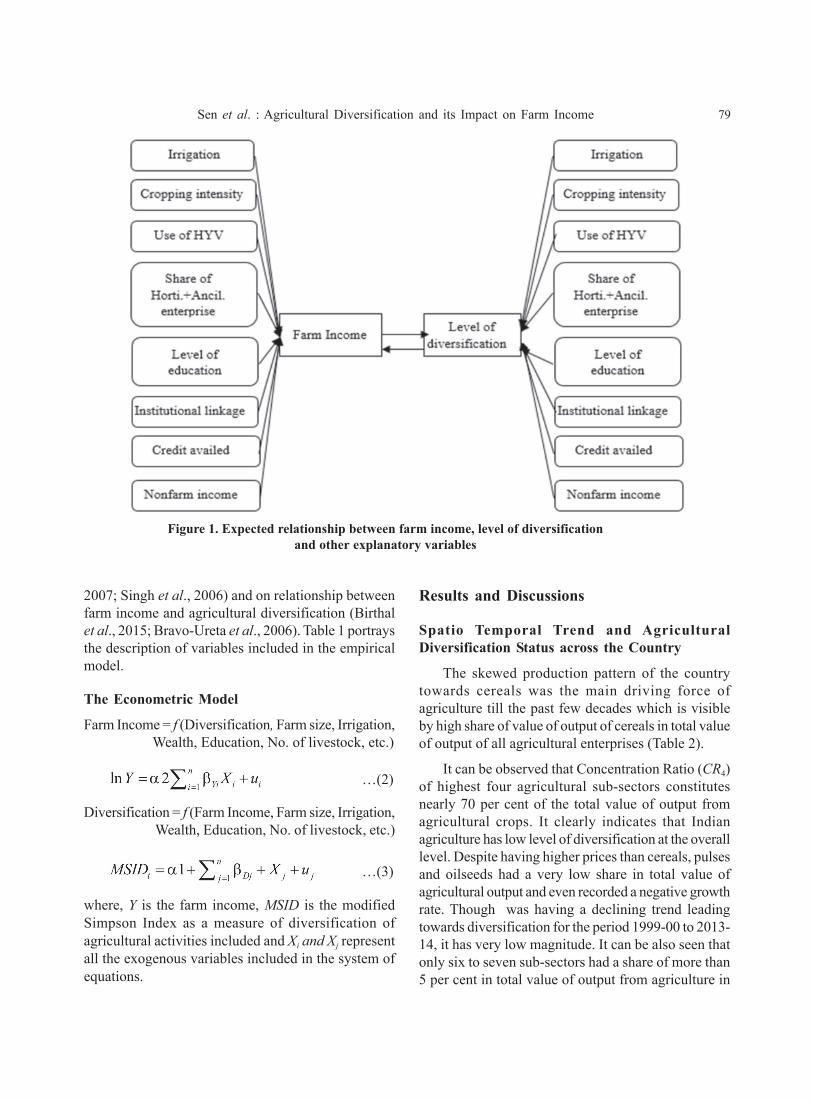
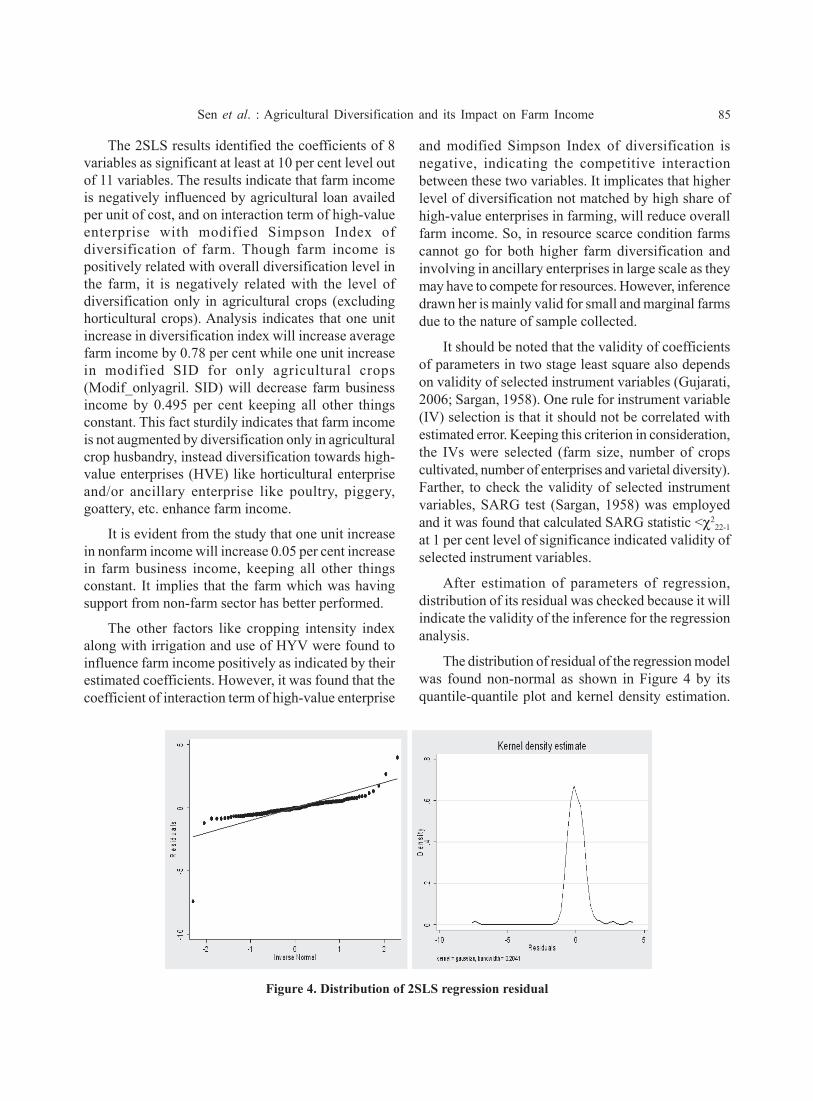
After estimation of parameters of regression,distribution of its residual was checked because it willindicate the validity of the inference for the regressionanalysis.

The distribution of residual of the regression modelwas found non-normal as shown in Figure 4 by itsquantile-quantile plot and kernel density estimation.

Figure 4. Distribution of 2SLS regression residual


In contrast to the case of OLS regression, where,normality of residual was a strict assumption fordrawing inference, the two-stage least square does notstrictly depends upon normality assumption of residual(Kelejian, 1971; Brown, 1990).

Economics of Agricultural Diversification on FarmIncome

Table 6 reveals that marginal farms had averageannual per family income of ` 36241, which is lessthan half compared to income of small and mediumfarmers. But conversely, marginal farms hadconsiderably higher per hectare farm income. It strictlydenotes marginal farms had a better efficiency inutilization of resources. Though average farm size isonly 0.358 ha for marginal farms, average number oflivestock per farm is 0.76. In addition to that, averageSID for marginal farms is also low (0.571) comparedto SID for small and medium farms (0.71 and 0.78). Itimplies that the level of agricultural diversification onlydoes not determine farm income in a strict sense; ahigher share of livestock enterprise will increase farmefficiency. It is more evident with the mean value of

returns over variable cost for marginal farms (2.34)which did not differing significantly from othercategories of farms.

Transversely, considering the scenario enterprise-wise (Table 7), it was found that the farms withhorticulture and livestock enterprises had the highestper hectare farm income, and returns to variable costratio. It was also seen that farms having livestockcomponent, could reap better returns compared to farmswhich relied only on agriculture. Agriculture,horticulture and livestock enterprise-mix was the mostprofitable and rational venture as indicated by farmincome and efficiency measure from Table 7. However,it is evident from Table 7 that with high level ofdiversification inclined towards horticulture andlivestock will augment farm income.

ConclusionThe paper has looked into the status and trend of

agricultural diversification across different states ofIndia and also at farm level for selected districts ofBihar. Alongside it has analysed the impact of

Table 6. Farm income and farm efficiency measure for different categories of farms based on size of holding

Farm category Farm Average Livestock SID Farm income Family income Returns(No.) farm size unit value (`/ha/ annum) (`/ha/ annum) to variable

(ha) (No./farm) cost (`)

Marginal 93 0.36 0.76 0.57 144511 36241 2.34Small 23 1.23 0.42 0.71 83888 74345 2.73Semi-medium 4 2.48 0.45 0.78 81072 93246 2.22& medium

Table 7. Farm income and farm efficiency measure for different categories of farms based on enterprise mix

Farming Farm Farm size Livestock unit SID Farm income Family income Returns toenterprises (No.) (ha.) (No./farm) value (`/ha/ annum) (`/ha/ annum) variable

cost (`)

Agri+ Horti 38 0.56 0.18 0.59 80879 40952 2.05Horti+ Livestock 11 0.13 0.86 0.42 234270 69474 3.1Agri + Horti + 43 0.57 0.73 0.67 116361 52584 2.68Livestock & ancill.Others 28 0.59 0.37 0.60 106915 48342 2.7Total 120 0.61 0.48 0.61 115813 52491 -

Note: #indicates number of marginal, small and semi-medium and medium farms


agricultural diversification on farm income. Over thestudy period, several changes have been observed incrop-mix and also in enterprise-mix across the states,although the overall level of agricultural diversificationstill differs noticeably which ranges from 0.61 (Punjab)to 0.89 (Karnataka) bracketing most of the states inmedium or high diversified states category. However,the crop diversification strategy which was intendedto provide wider choice of production of different crops,was lacking in its impressions over time because cropdiversification though reduces risks associated inagriculture (Bradshaw et al., 2004; Elbers et al., 2007),it is not regarded as a measure of income augmentationin the strict sense.

The cross-sectional analysis for selected districtsof Bihar revealed that marginal farmers in general didnot have sole source of income as crop husbandry asthey have diversified towards ancillary enterprises, viz.small poultry, duckery, piggery or goatery. Due to usingan integrated farming approach, these ancillaryenterprises were proving to be highly profitable in smallscale with sufficiently low degree of risks due to itssmall magnitude of span of operation. The study hasconcluded that along with over all agriculturaldiversification, irrigation, cropping intensity, andhigh-value and ancillary enterprises will supplementfarm income and will help to achieve farm incomesecurity.

Policy ImplicationsThe study has shown that diversification of farm

business does not always increase farm income,because, it depends on the direction of diversification.Therefore, with an integrated farming approach,diversification of farm by adopting ancillary,horticulture and other high-value enterprises likemushroom, etc. should be promoted to increase farmincome. For the resource-poor marginal and smallfarmers, income will increase with diversificationtowards high-value enterprises complemented withsmall-scale ancillary enterprises. Surprisingly, thoughhaving high profitability, these ancillary enterpriseswere not being popular among the higher-resourcefarmers, because of social stigma associated with theseenterprises and are considered to be inferior enterprisesbounded only in low caste groups. Specific policyintervention is needed to deal with it with significantpromotional and extension activities.

AcknowledgementThe paper is based on the M.Sc. thesis entitled

“Economic Analysis of Agricultural Diversification andits Impact on Farm Income in Bihar” submitted to PGSchool, ICAR-IARI, New Delhi, by the first authorunder the chairmanship of the second author. Theauthors thank the anonymous referees for theirconstructive comments.

ReferencesBirthal, P. S., Roy, D., and Negi, D. S. (2015) Assessing the

impact of crop diversification on farm poverty in India.World Development, 72: 70-92.

Birthal, P.S., Joshi, P.K. and Gulati, A. (2007) Verticalcoordination in high-value food commodities:Implications for smallholders. In : AgriculturalDiversification and Smallholders in South Asia, Eds :P.K. Joshi, Ashok Gulati and Ralph Cummings (Jr).Academic Foundation, New Delhi.

Bradshaw, B., Dolan, H. and Smit, B. (2004) Farm-leveladaptation to climatic variability and change: Cropdiversification in the Canadian prairies. ClimaticChange, 67(1): 119-141

Bravo Ureta, B.E., Solis, D., Cocchi, H., and Quiroga, R.E.(2006) The impact of soil conservation and outputdiversification on farm income in Central Americanhillside farming. Agricultural Economics, 35(3): 267-276.

Brown, R.L. (1990) The robustness of 2SLS estimation ofa non-normally distributed confirmatory factor analysismodel. Multivariate Behavioral Research, 25(4): 455-466.

Cochrane, N., Schmitz, A. and Bojnec, S. (1994) Agriculture:diversification and productivity: In: Privatization ofAgriculture in New Market Economies: Lessons fromBulgaria. Springer, Netherlands. pp. 23-53.

Directorate of Economics and Statistics, Government ofIndia, http://eands.dacnet.nic.in/

Elbers, C., Gunning, J. W. and Kinsey, B. (2007) Growthand risk: Methodology and micro evidence. The WorldBank Economic Review, 21(1): 1-20.

Feder, G., Just, R. E. and Zilberman, D. (1985) Adoption ofagricultural innovations in developing countries: Asurvey. Economic Development and Cultural Change,33(2): 255-298.

Gavian, S. and Fafchamps, M. (1996) Land tenure andallocative efficiency in Niger. American Journal ofAgricultural Economics, 78(2): 460-471.


Gujarati, D. (2006) Essential of Econometrics. 3rd edition,McGraw- Hill, New York.

Hardaker, J.B. (1997) Guidelines for the Integration ofSustainable Agriculture and Rural Development intoAgricultural Policies (No. 4). Food and AgricultureOrganization, Rome.

Hossain, Z., Gurr, G. M. and Wratten, S. D. (2001) Habitatmanipulation in lucerne (Medicagosativa L.): Stripharvesting to enhance biological control of insect pests.International Journal of Pest Management, 47(2): 81-88.

IFPRI (2003) Income diversification and poverty in theNorthern Uplands of Vietnam.Markets, Trade andInstitutions Division, IFPRI,Washington, DC.

Joshi, P.K., Gulati, A., Birthal P.S. and Tiwari L. (2004)Agriculture diversification in South Asia: Pattern,determinants and policy implications. Economic andPolitical Weekly, 39 (24): 2457-2467.

Kelejian, H.H. (1971) Two-stage least squares andeconometric systems linear in parameters but nonlinearin the endogenous variables. Journal of the AmericanStatistical Association, 66(334):373-374.

Krupinsky, J. M., Bailey, K. L., McMullen, M. P., Gossen,B. D. and Turkington, T. K. (2002) Managing plantdisease risk in diversified cropping systems. AgronomyJournal, 94(2): 198-209.

Kumar, S., and Gupta, S. (2015) Crop diversificationtowards high-value crops in India: A state levelempirical analysis. Agricultural Economics ResearchReview, 28(2): 339-350.

Morris, C. and Winter, M. (1999) Integrated farmingsystems: the third way for European agriculture?. LandUse Policy, 16(4): 193-205.

Petit, M., and Barghouti, S. (1992) Diversification:challenges and opportunities. Trends in AgriculturalDiversification: Regional Perspectives. World BankTechnical Paper (180).

Pingali, P.L., and Rosegrant, M.W. (1995) Agriculturalcommercialization and diversification: Processes andpolicies. Food Policy, 20(3): 171-185.

Pretty J. (1994) Alternative systems of inquiry for asustainable agriculture. IDS Bulletin 25: 37-49.

Sargan, J.D. (1958) The estimation of economicrelationships using instrumental variables.Econometrica: Journal of the Econometric Society, 393-415.

Singh, N.P., Kumar, R. and Singh, R.P. (2006)Diversification of Indian agriculture: Composition,determinants and trade implications. AgriculturalEconomics Research Review, 19: 23-26.

Smith, R.G., Gross, K.L. and Robertson, G.P. (2008) Effectsof crop diversity on agro-ecosystem function: Cropyield response. Ecosystems, 11(3):355-366.

Tilman, D., Cassman, K.G., Matson, P.A., Naylor, R. andPolasky, S. (2002) Agricultural sustainability andintensive production practices. Nature, 418(6898): 671.

Vyas, V.S. (1996) Diversification in agriculture: Concept,rationale and approaches. Indian Journal ofAgricultural Economics, 51(4): 636-643.

Weiss, C.R. and Briglauer, W. (2000) Determinants andDynamics of Farm Diversification (No. 0002). FEWorking paper/Universität Kiel, Department of FoodEconomics and Consumption Studies.

Zhu, Y., Chen, H., Fan, J. and Wang, Y. (2000) Geneticdiversity and disease control in rice. Nature, 406(6797):718.

Documents

Agricultural Diversification and its Impact on Farm …ageconsearch.umn.edu/record/265244/files/7-B-Sen.pdfRelating it to farm level situation, the primary survey in Banka and Bhagalpur