Embed Size (px)
Citation preview

Agricultural Groundwater Markets:Understanding the Gains from Trade and the Role
of Market Power∗
JOB MARKET PAPER
The latest version is available for download at ellen-bruno.com/research.
Ellen M. Bruno†
December 20, 2017
AbstractThis paper models and quantifies the efficiency gains from using market-basedinstruments relative to command and control to manage groundwater. A the-oretical model of a groundwater market is developed to show how the mag-nitude and distribution of the gains from trade change as market structurevaries. Market structure is a key consideration because the presence of largegrower-shippers and/or competition among a few water agencies on a sharedbasin may be defining components of future groundwater markets. Using datafrom a groundwater basin in southern California, this paper demonstrates theexistence of large gains from trade, despite the potential for market power.Importantly, the price elasticity parameter used to calibrate the model is gen-erated with a fixed-effects econometric model that utilizes well-level panel dataon groundwater extraction and exploits temporal and cross-sectional variationin extraction prices. Simulations that vary market conditions show that re-sults generalize to other groundwater basins.
∗I am grateful to Richard Sexton and Katrina Jessoe for their guidance and support. I wouldalso like to thank Pierre Mérel, Michael Hanemann, Richard Howitt, James Wilen, Daniel Sumner,Jeffrey Williams, and Kevin Novan for helpful comments and suggestions. This paper benefitedfrom participant comments at presentations at the Western Agricultural Economics Associationand the Agricultural and Applied Economics Association annual meetings, the University of West-ern Australia, and the Australian Agricultural and Resource Economics Society. Funding for thisresearch came from: Giannini Foundation of Agricultural Economics, UC Water Security andSustainability Research Initiative funded by the UC Office of the President (Grant No. MR-15-328473), and the National Science Foundation Climate Change, Water, and Society IGERT (DGENo. 1069333).†Ph.D. Candidate, Department of Agricultural and Resource Economics, University of Califor-
nia, Davis. Email: [email protected].
1 Introduction
Improved management of water resources is becoming increasingly important in
the face of climate change. We expect to see more variability in precipitation,
with droughts, floods, and other extreme climate events occurring more frequently
(Kunkel et al. 2013). Because groundwater serves as a buffer to fluctuations in
surface water supplies, it can significantly reduce the cost of climate change for
agriculture. However, many groundwater basins worldwide have seen declines in
groundwater storage over time because groundwater is extracted at a rate faster
than it can be replenished (Rodell, Velicogna, and Famiglietti, 2009). This is largely
due to the lack of regulation of this common property, open-access resource. Since
groundwater management will have impacts on agriculture, attention must be given
to the choice of policy instrument.
Nowhere are concerns about groundwater management more pronounced than in
California. Groundwater accounts for 40% of the agricultural water supply on aver-
age (California Department of Water Resources, 2016) and several areas throughout
the state have seen significant declines in groundwater storage (Faunt, Belitz, and
Hanson, 2009). In recognition of the value in maintaining a reliable groundwater
supply, California passed legislation in 2014 that provides a statewide framework for
local agencies to manage groundwater. The 2014 Sustainable Groundwater Manage-
ment Act requires overdrafted basins throughout California to reach and maintain
long-term stable groundwater levels. However, California’s new groundwater law
is silent as to how groundwater agencies should achieve sustainability, even though
the cost effectiveness of different policy instruments may vary substantially. With
minimal assumptions on permit market structure, this paper evaluates the efficiency
gains of groundwater markets relative to a command-and-control regime for manag-
ing groundwater.
1

Economists have espoused the merits of market-based instruments to manage the
environment (e.g., Goulder and Parry 2008) and growing empirical work points to
substantial cost savings from the deployment of market-based instruments relative
to command and control policies for air pollution (e.g., Fowlie, Holland, Mansur
2012). Less is known, however, about the performance of economic instruments for
managing water. The existing literature focuses on the gains from surface water
transfers, suggesting that there are large benefits from the reallocation of water
from low-value to high-value users (e.g., Vaux and Howitt 1984; Hearne and Easter
1997). However, these arguments often rest on questionable assumptions regarding
competition, information, and the availability of substitutes, and have yet to be
empirically corroborated.
The performance of market-based instruments is further complicated by the pres-
ence of other market failures. Market structure will be an important feature to
consider when evaluating the merits of markets to manage groundwater. Driven by
the presence of large, vertically integrated farming-shipping operations, formation of
coalitions among buyers or sellers, and/or competition among a few water agencies
on a shared basin, market power in trading may occur due to the concentration of
permits among a handful of buyers or sellers; this will decrease the gains from allow-
ing groundwater trade and could have significant implications for the distribution
of benefits from groundwater markets. This paper addresses the question of how
either seller or buyer market power affects the efficiency gains and distributional
consequences from groundwater trade. An evaluation of the merits of groundwater
trading in the presence of imperfect competition contributes to the policy discussion
regarding the potential role of markets to manage groundwater.
In this paper, I first develop a theoretical framework to study agricultural ground-
water use and trading. After deriving unconstrained groundwater demand functions,
property rights for pumping are allocated such that the aggregate use is restricted.
2

I then derive permit demand and supply curves, which are used to quantify the
gains from trade. Using a flexible model framework that can reflect any degree of
buyer or seller market power in the permit market for groundwater, I identify the
relationship between market power and the efficiency of water trading. Simulations
show how the total efficiency gains and the distribution of benefits between buyers
and sellers changes with market structure. Results based on linear groundwater
demand curves show that the total impacts of market power are relatively small,
however, the distributional impacts are considerably larger. Distributional impacts
are important from a policy perspective because they may influence the political
feasibility of implementing groundwater markets. I show that those with market
power (whether as buyers or sellers) may be able to capture large shares of the gains
from trade.
The contribution of the theoretical model is twofold. First, this paper extends a
branch of literature that evaluates the impacts of market power in permit markets
to include groundwater. Stemming from the seminal paper by Hahn (1984), this
literature considers the initial distribution of property rights, strategic behavior of
competitors, and impacts in the final product market, with applications to fisheries
and pollution (e.g., Misiolek and Elder 1989; and Montero 2009). Second, this paper
relaxes assumptions regarding market structure to more broadly characterize the
impacts of imperfect competition. Whereas previous literature makes assumptions
on market structure, e.g., Cournot competition, or one or two dominant firms with
a competitive fringe (Westskog 1996; and Montero 2009), this paper uses a flexible
framework for imperfect competition in the permit market, allowing the model to
depict the entire range of possible market power settings for either buyer or seller
power. A key feature of this analysis is the demonstration of market power impacts
via simulations that vary a flexible market power parameter.
The model is applied to a groundwater basin in southern California that under-
3

lies the Coachella Valley, a major production region for citrus, dates, grapes, and
other vegetable row crops. I contribute to the literature on water markets by esti-
mating the gains from groundwater trade for the water district serving this area. A
novel feature of this application is that all model parameters are either constructed
or estimated using observational data from Coachella Valley. Importantly, the price
elasticity of demand for groundwater in the Valley is estimated with econometric
methods that utilize the panel structure of monthly, well-level groundwater extrac-
tion and price data. Results show that the economic surplus with trade is over twice
as large as that under command and control.
The estimation of the price elasticity of groundwater demand represents another
key contribution of the paper. A reliable estimate of this elasticity is essential to
assessing the potential of price as a tool to manage groundwater. Previous estimates
of agricultural water demand elasticities have varied widely, ranging from −0.001 to
−1.97 (Scheierling, Loomis, Young 2006). Of these previous estimates, those that
used groundwater extraction data have (1) relied on estimates of pumping costs for
price because groundwater itself is typically free of charge and (2) focused on areas
without surface water access (e.g. Hendricks and Peterson 2012; Gonzalez-Alvarez,
Keeler, and Mullen 2006). The Coachella Valley Water District is unique because it
deploys a location-based volumetric pricing scheme for groundwater. This ground-
water extraction price allows me to estimate a price response without attenuation
and amplification bias due to incomplete information on energy costs to extract
groundwater (Mieno and Brozovic 2017). Furthermore, data on surface water use
enables the model to control for substitution and isolate the price response in ground-
water use. Exploiting temporal and cross-sectional variation in prices, I provide an
estimate of the price elasticity of groundwater demand for the Coachella Valley that
is the first of its kind to not rely on estimates of pumping cost for price.
In the following section, I provide background on California’s 2014 Sustainable
4

Groundwater Management Act and the avenues through which market power may
arise in groundwater markets. In Section 3, a theoretical model of agricultural
groundwater use is developed. I derive unconstrained groundwater demand func-
tions and then assign property rights for pumping. Section 4 introduces trade;
permit demand and supply curves are derived. Within this framework, I compare
the perfectly competitive and imperfectly competitive solutions and determine the
effects of market power on market outcomes and distribution of welfare. Section
5 contains an application to California’s Coachella Valley. This is followed by a
simulation analysis in Section 6 that tests the sensitivity of these results. The final
section concludes.
2 Background
Groundwater is a significant component of California’s water supply that has his-
torically been unmeasured and unmanaged. Prompted by years of severe drought,
the California state legislature passed a landmark groundwater law in 2014 that
provides a statewide framework for local groundwater agencies to coordinate data
management and organize basin management plans to eliminate overdraft. The law
applies to 127 of 515 basins in California, which account for 96% of the groundwater
pumping in the state. The Sustainable Groundwater Management Act (SGMA)
gives local agencies the authority and flexibility to correct overdraft conditions in a
variety of ways.
Water agencies governing overdrafted basins will likely need to reduce basin-wide
pumping to achieve groundwater sustainability targets. Regulators may choose to
do this by restricting individual pumping volumes, after establishing property rights
for groundwater. However, the assignment of property rights for groundwater use
will cause efficiency loss in the absence of water trading, if the regulating agency
5

lacks perfect information and/or faces legal restrictions to setting allocations.1 Thus,
groundwater trading may emerge as one possible avenue for reaching basin sustain-
ability targets. Groundwater markets have the added benefit of eliminating uncer-
tainty in reaching a target, as compared to other economic instruments like taxes.
Prior to implementation of a trading regime, it is important to understand the mag-
nitude and distribution of benefits of groundwater markets, particularly given the
likely presence of market power. As groundwater markets become more prevalent
in California and elsewhere, determining the competitive outlook for these markets
and understanding the consequences resulting from any market power abuses will
be one of the fundamental challenges facing policymakers.
Due to the nature of water institutions and the market structure of agricul-
tural production in California, market power may be a defining component of future
groundwater trading. Several structural elements may give rise to imperfectly com-
petitive groundwater markets. For many groundwater basins in California, multiple
groundwater management agencies are emerging to jointly manage the groundwater
on a shared basin. If trading then occurs among a handful of groundwater agencies,
it will be characterized by a small-numbers problem. Also, a significant amount of
current surface water trading and groundwater banking (artificial aquifer recharge)
in California is organized at the district or county level among districts on behalf of
the farmers within their service areas. Water districts may be able to act as implicit,
legal cartels that are able to influence price in purchases or sales of groundwater.
Even under the authority of a single agency for a given groundwater basin,
market power will be a concern if only a few players are active on one side of the
market. The agricultural sector has seen significant structural change over the last
several decades, leading to fewer, larger, and vertically integrated farming-shipping1California’s correlative rights doctrine, which gives landowners the right to use the ground-
water underneath his or her land, may determine how property rights are allocated under theSGMA.
6

operations. Most groundwater rights in California are overlying rights, which are
based on ownership of the land above the aquifer and give the landowner the right
to pump. It is likely that permits for pumping, when properly defined to facilitate
transfers, will be allocated based off land size, causing the concentration of permits
in the hands of the large players. Furthermore, the absence of legal restrictions
regarding the formation of coalitions among buyers or sellers may lead to groups
of players coordinating interests and dominating the market. Given that trading
will be restricted to the boundaries of a given groundwater basin, the structure
of California agricultural production and the legal environment regarding coalition
formation may give rise to consolidation of groundwater rights when they become
properly defined under the SGMA.
In this paper, I focus specifically on the Coachella Valley Groundwater Basin
in southern California, which is an ideal setting for many reasons. Multiple water
agencies in the Coachella Valley have been approved by the California Department
of Water Resources as “Groundwater Sustainability Agencies” to jointly manage the
Coachella Valley Groundwater Basin over the coming years. They are required to
work together to reach sustainability targets for the entire basin, e.g., by trading
groundwater pumping rights among agencies. Additionally, since the Valley is home
to large grower-shippers like Grimway Farms for vegetables and Sun World for table
grapes, the concentrated structure of Coachella’s agricultural production may en-
able the exercise of market power in an emergent permit market. Lastly, access to
the Coachella Valley Water District’s data on monthly groundwater extraction and
price by well enables me to estimate the groundwater demand elasticity, a necessary
component to quantifying the gains from trade.
7

3 Modeling Framework
I develop a theoretical model for studying agricultural groundwater use and trading.
The model is framed as if a single authority governs an entire groundwater basin,
the groundwater basin defines the market, and permit trading occurs among farm-
ers. However, this framework may be adapted to represent an aquifer with several
governing agencies where trade occurs among agencies. Within this framework, I
investigate the magnitude of the gains from trade, the distribution of benefits among
traders, and how both are affected by market power.
We build up from an unmanaged, open-access groundwater setting to tradable
property rights for pumping. Throughout, we assume farmers draw groundwater
from a common aquifer. For simplicity, we assume there are two types of farmers
pulling from the aquifer, low (L) and high (H), that are homogeneous within their
type. Each produces a single output. Farmers of type L grow a low-value crop, such
as rice or cotton, with individual production functions denoted qLj = gj(xLj, y).
Farmers of type H grow a high-value crop, e.g., a produce commodity or tree nut,
with individual production functions denoted qHj = fj(xHj, z).2 Production func-
tions are assumed to exhibit diminishing marginal productivity to variable inputs.
The variable x represents applied groundwater and y and z are other inputs to
production.
There are Ni identical individuals j = 1, ...Ni within each type i ∈ H,L. We
distinguish the two types such that growers of the high-value crop have a higher will-
ingness to pay for water at any given quantity of groundwater. To account for system
distributional losses, pumped groundwater is distinguished from the amount of wa-
ter applied to the crop. Aggregate water quantities are denoted by X and x with-2This formulation assumes farmers have already preselected into producing certain crops, e.g.,
based on heterogeneous ability levels or land quality. This is a short-run analysis. Changes incropping patterns that might occur over time due to alternative groundwater management regimesare not considered.
8

out individual-specific or type-specific subscripts, where uppercase is for pumped
groundwater and lowercase is for applied groundwater. That is, X = XH +XL and
x = xH +xL, where total H-type pumped water is XH =∑NH
j=1XHj (uppercase) and
total H-type applied water xH =∑NH
j=1 xHj (lowercase). The relationship between
pumped and applied water is given by the efficiency parameter δ with 0 < δ < 1 such
that xi = δXi. We must distinguish pumped groundwater from applied groundwater
because applied water is what determines production outcomes, whereas pumped
groundwater is the good to be traded.
The marginal pumping cost of water is denoted by c(X) and is an increasing
function of the total amount pumped out of the aquifer due to reducing the water
table as more water is pumped. Marginal pumping costs are positive, increasing,
and differentiable, i.e. c(X) > 0 and c′(X) > 0. When individual pumping is
small relative to the basin total, farmers face the same costs and take the marginal
pumping cost as given, but collectively their decisions determine basin-wide pumping
costs.3
3.1 Open-Access Groundwater Use
I begin with the profit maximization problem for farmers in the unmanaged, open-
access case. Total costs of production come from groundwater pumping costs and
the costs of other inputs, such as fertilizers and pesticides. The price of groundwater
is denoted wx and the prices of the other inputs are denoted wy and wz. When the
aquifer is an unmanaged common-pool resource, the price of groundwater equals the
marginal pumping cost, which individual users regard as constant, and is denoted
by wx = c. Firms are assumed to choose inputs (xH , z) for H types or (xL, y) for L3One possible extension of this work is to expand on this farm-level groundwater optimization
problem by allowing individual firms to believe they pump enough to influence their own pumpingcosts. This may be because they are big enough to impact the water table with their consumptionor they pump enough to create a cone of depression at the site of a well.
9

types to maximize farm profits, where Pi is the output price for the crop produced
by type i, i ∈ L,H. An individual of type H faces the following profit maximization
problem:
maxxHj ,z
πHj = PHfj(xHj, zj)− cxHjδ− wzzj. (1)
The first-order conditions for each of the H types are:
PH∂fj(xHj, zj)
∂xHj=c
δ, PH
∂fj(xHj, zj)
∂zj= wz (2)
and are similar for each of the L types. Solving for xHj and xLj reveals the
groundwater demand curves for each farmer j, which are functions of crop output
price, input prices, and the marginal pumping cost of groundwater: xHj(PH , wz, c),
xLj(PL, wy, c). When optimizing, farmers equate the marginal value product of an
additional unit of groundwater to its price, which here is the marginal pumping
cost adjusted by the efficiency parameter. These expressions recognize that a unit
pumped yields less than a unit applied due to inefficiencies in delivery.
3.2 Competitive Equilibrium
The market equilibrium comes from equating the aggregate water demand relation-
ships across both types with the aggregate water supply relationship. Aggregate ap-
plied water demands are given by xH+xL =∑NH
j=1 xHj+∑NL
j=1 xLj. The aggregate wa-
ter supply relationship is just marginal pumping costs as a function of total pumping,
adjusted by system distributional losses. If we define equilibrium pumping quantities
and costs by writing x∗H = xH(PH , wz, w∗x), x∗L = xL(PL, wy, w
∗x), and w∗x, respec-
tively, then the equilibrium condition is given by c(X∗) = c(x∗H(w∗
x)
δ+
x∗L(w∗x)
δ) = w∗x.
To obtain analytical solutions, I assume aggregate demands for applied water
are linear and parallel such that the H type demand curve is higher than that of the
10

L type for all quantities of applied water.4 As shown in (3), we have intercepts of γ
and αγ for the H and L types, respectively, with 0 < α < 1, and slope coefficients
assumed to be the same, given by β2:
xH = γ − β
2wx and xL = αγ − β
2wx. (3)
Throughout, I assume marginal pumping costs are increasing and linear with positive
intercept and slope coefficients, c(X) = θ + µX with θ, µ > 0. Aggregate applied
water demand is the sum of the total water demands from each type: x = xH +xL =
(α + 1)γ − βwx. The intersection of this function with the supply relationship for
applied water, wx = θ + µδx, reveals the competitive, open-access equilibrium price
(w∗x) and quantity (x∗):
x∗ =δγ(α + 1)− δβθ
δ + βµ,w∗x = θ + µ(
γ(α + 1)− βθδ + βµ
). (4)
In what follows, I invoke normalizations (units of measurement for price and wa-
ter quantity) such that the competitive market equilibrium price (i.e., pumping cost)
and quantity are each equal to one (x∗, w∗x) = (1, 1). Evaluated at the competitive
equilibrium, the absolute value of the demand elasticity is given by η = β and the
supply elasticity is ε = δµ.5 Given the normalizations, we can rewrite the demands
for L and H types and the aggregate supply relationship as functions of readily
interpretable parameters: the supply and demand elasticities evaluated at the com-
petitive equilibrium, ε and η respectively, the demand shift parameter, α ∈ (0, 1),
reflecting differences in water demands between H and L types, and the water distri-4I choose to define functional forms for water demands at the aggregate level for analytical
simplicity. I divide aggregate demands by the number of agents in each type to reveal individualwater demands.
5The elasticity of demand is given by η = |∂xD
∂wx
wx
xD | = β evaluated at the equilibrium (1, 1)
with xD(wx) = γ(α + 1) − βwx. The elasticity of supply is given by ε = ∂xS
∂wx
wx
xS = δµ at (1, 1)
where xS(wx) = δµwx−
δµθ. These imply the following substitutions, which are used to rewrite the
original expressions: β = η, θ = 1− 1ε , γ = 1+η
1+α , µ = δε .
11

bution efficiency parameter δ ∈ (0, 1). This substitution eliminates the dependence
of the model on units of measurement, as all parameters defining the market are
pure numbers. Restating all solutions with respect to this normalization, we have
the following:
Equilibrium groundwater quantity and price: (x∗, w∗x) = (1, 1)
Aggregate high-type demand: xH = 1+η1+α− η
2wxH
Aggregate low-type demand: xL = α( 1+η1+α
)− η2wxL
Individual farm marginal value products:
MV PHj = 2η( 1+η
1+α−NHxHj)
MV PLj = 2η(α( 1+η
1+α)−NLxLj)
Aggregate inverse groundwater supply: wx = (1− 1ε) + 1
εx.
3.3 Establishing Property Rights for Groundwater
Let us now assume that a regulatory agency intervenes by establishing non-tradable
property rights for pumping. To induce conservation, the agency sets an aggre-
gate endowment that is less than the amount pumped in the open-access scenario.
Without the ability to trade, both types must reduce pumping to their assigned
allocation. Although it is possible to arrive at the socially optimal solution through
a discriminatory set of water allocations where each type is allocated the amount
it would pump in the socially optimal setting, we logically assume the regulator
lacks such information or the political ability or legal right to implement such an
allocation.6 Instead we assume that allocations are based on some simple rule, such
as equal amounts to each farmer or on a pro rata basis by land size, rendering it
highly unlikely that the allocation equates marginal value products across types.
Suppose each farmer receives an initial groundwater allocation, denotedX0ij, that
6Recall that most groundwater rights in California are overlying rights, meaning the legal rightsto groundwater are generally tied to landholdings.
12
is assumed to be the same across farmers within each farmer type. In the absence of
markets, each farmer is constrained to choose xij(·) ≤ δX0ij. Assuming farmers take
pumping costs as given, we have the following constrained optimization problem for
all individual H types, where λH,j is the Lagrange multiplier associated with the
constraint for individual j:
maxxHj ,zj ,λHj
πHj = PHfj(xHj, zj)− cxHjδ− wzzj − λHj(xHj − δX0
Hj). (5)
The Kuhn-Tucker conditions are:
PH∂fj(xHj, zj)
∂xHj− c
δ− λHj ≤ 0 and xHj(PH
∂fj(xHj, zj)
∂xHj− c
δ− λHj) = 0 (6)
PH∂fj(xHj, zj)
∂zj− wz ≤ 0 and zj(PH
∂fj(xHj, zj)
∂zj− wz) = 0 (7)
xHj − δX0Hj ≤ 0 and λH(xHj − δX0
Hj) = 0 (8)
λHj ≥ 0, xHj ≥ 0, zj ≥ 0. (9)
Any meaningful allocation of property rights in this setting must cause a binding
constraint on pumping, at least for the high types. Therefore, in equilibrium we
must have a strictly positive shadow price λ∗Hj > 0; at the constrained optimum,
the H types utilize the full allocation, i.e. x∗Hj = δX0Hj. The constrained maximiza-
tion problem and associated Kuhn-Tucker conditions are similar for the L types.
However, the constraint does not necessarily bind for the L types, even though it
binds for the H types, because L types have a lower willingness to pay for ground-
water at any quantity than the H types. In what follows, however, I focus on the
case where the allocation also binds for the L types.7
If we assume the constraint binds for both types, we get the following expressions7I do this for simplicity, to avoid the discontinuity associated with the kinked supply curve
that would result if the allocation was only sometimes binding for the L types.
13

for the shadow prices:
λ∗Hj = PH∂fj(δX
0Hj, zj)
∂xH− c
δ(10)
λ∗Lj = PL∂gj(δX
0Lj, yj)
∂xL− c
δ. (11)
This framework is important for establishing the baseline for a water market to
emerge; we derive the excess demand/excess supply functions for permits based on
this constrained equilibrium. A necessary condition for water markets to emerge is
that the shadow price for the H types must be strictly greater than that of the L
types at the constrained equilibrium. Applying functional forms to equations (10)
and (11), I characterize the necessary condition in terms of aggregate demands for
each type. Since farmers are identical within each type, we drop the individual-
specific subscript and define X0i as the aggregate endowment for one type, such that
X0i = NiX
0ij. The shadow prices become:
λ∗H =2
η(1 + η
1 + α− δX0
H)− c
δ(12)
λ∗L =2
η(α(1 + η)
1 + α− δX0
L)− c
δ. (13)
Equation (14), which is equivalently the difference in marginal value products
between types evaluated at the optimum x∗ij = δX0ij, gives the necessary condition
for trading to occur:
λ∗H − λ∗L = MV PH(δX0H)−MV PL(δX0
L)
=2
η[(1− α)(1 + η)
1 + α+ δX0
L − δX0H ] > 0.
(14)
When equation (14) holds, we know there exists some set of positive permit
prices where trading will occur. Thus, in the subsequent analysis we assume (14) is
satisfied. I define Ω = (1−α)(1+η)1+α
+ δX0L − δX0
H for simplicity. Rearranging equation
14

(14),(1− α)(1 + η)
1 + α> δ(X0
H −X0L), (15)
shows that when the difference in open-access quantity demanded between the two
types exceeds the difference in their effective allocation, there will be trade. Since
the term, (1−α)(1+η)1+α
, is positive for all values of α and η, an initial allocation which
distributes permits equally between types is sufficient for trading to occur.
4 Tradable Property Rights
I now introduce trade by using the groundwater demand functions and the ex-
ogenous allocation of pumping rights to create excess demand and excess supply
functions for pumping permits. Let us consider a homogeneous product market for
groundwater permits where two types buy and sell water pumping permits. Selling
or supplying groundwater in this context is simply being paid not to pump up to
one’s allocation of groundwater. Therefore, we define trade in terms of pumped
groundwater, as opposed to applied groundwater. Let ρ represent permit price and
XTi be the quantity of permits traded by type. Each farmer receives an allocation
appropriate for his type and relates this to his input demand for water to formulate
excess demand/excess supply functions. We define the excess function for farmer j
in type i, denoted Eij(ρ), as the difference between his water demand (for pumped
water) at price ρ and water allowance, X0ij:
Eij(ρ) ≡ xij(ρ)
δ−X0
ij. (16)
If Eij(ρ) > 0, individual j has excess demand at groundwater price ρ because his
water demand exceeds his endowment of water rights. If Eij(ρ) < 0 at groundwater
price ρ, then individual j has excess supply because his water demand is less than
15

Figure 1: Excess Supply and Demand for Groundwater
his allocation. As before, we drop the individual-specific subscript and define X0i as
the aggregate endowment for one type since farmers are identical within each type.
Given that (14) holds, the H types will be net demanders and the L types will be
net suppliers in the water market. Applying functional forms to the excess equation
(16) obtains the following excess demand and excess supply curves:
Excess Demand: XTH =
1
δ(1 + η
1 + α)−X0
H −η
2δρ (17)
Excess Supply: XTL = X0
L −1
δ
α(1 + η)
1 + α+
η
2δρ (18)
The excess demand/supply curves are functions of the demand elasticity and
other parameters from the profit maximization problems. Fixing these exogenous
parameters at particular levels fixes the intercepts and slopes for the excess functions.
Figure 1 shows a graphical derivation of excess supply and excess demand for permits
from linear aggregate groundwater demands for the two types, which are labeled
16

Xi. The initial endowment of pumping rights is equal between types (X0L = X0
H), as
shown by the vertical line. ED(XTH) denotes inverse excess demand of permits for
the H types and ES(XTL ) denotes inverse excess supply of permits for the L types.
In equilibrium, the L-type farmers sell permits to the H-type farmers. In Figure
1, (ρ∗, XT ∗) denote the market-clearing permit price and quantity pumped under
perfect competition.
4.1 Perfectly Competitive Solution
Equating excess demand of equation (17) and excess supply of equation (18) yields
the following market-clearing price (ρ∗) and quantity (XT ∗) under perfect competi-
tion:
(XT ∗, ρ∗) = (
Ω
2δ,
1
η(1 + η − δ(X0
H +X0L))). (19)
The presence of the permit market alters the farmers’ optimization problems.
Marginal pumping costs now consist of the permit equilibrium price plus the physical
marginal pumping costs, adjusted by the efficiency parameter. Additional benefits
are captured by farmers when we allow agents to buy and sell excess pumping rights.
The gains from trade are given by the following expression, denoted G, which is
calculated as the sum of consumer and producer surplus in the permit market:
G =
∫ XT∗
0
ED(τ)− ES(τ)dτ =Ω2
2δη. (20)
Welfare in the permit market depends on the demand elasticity, the demand shift
and efficiency parameters, and the original endowment of property rights to both
types. It is strictly positive by (14), demonstrating the existence of net benefits
from voluntary trading. This area is shown in Figure 1 by the shaded triangle.
For use in the sensitivity analysis in Section 6, we also express the gains as a
percent increase from the surplus under non-tradable property rights for pumping,
17

i.e. command and control. Surplus under the command and control scenario is given
by (δX0H)2+(δX0
L)2
ηand calculated from the area under the demand curves and above
price when types are restricted to pumping X0i . The percentage increase in gains
due to trading relative to the no-trade scenario is given by following expression:
%4 =Ω2
2δ
(δX0H)2 + (δX0
L)2∗ 100. (21)
4.2 Imperfectly Competitive Solutions
Next, we evaluate how groundwater markets are impacted by market power. We
focus on within-basin market power with two cases: (1) a small number of sellers
exercise oligopoly power over many buyers (NL small, NH large) and (2) a small
number of buyers exercise oligopsony power over many sellers (NH small, NL large).
In the first case, the H types are assumed to behave competitively. In the second
case, sellers are competitive while permit buyers are not.
A convenient way to introduce either buyer or seller market power into our model
is to introduce market power parameters ξ and θ, which lie on the unit interval and
are interpreted as measures of market competitiveness. Various papers have used
this approach (e.g. Suzuki et al. 1994; Zhang and Sexton 2002). This framework
allows for the complete range of competitive outcomes among buyers and sellers
to be represented. For example, ξ, θ = 0 gives the perfectly competitive solution
in (19), while ξ = 1, θ = 0 gives the seller monopoly solution, and θ = 1, ξ = 0
depicts buyer monopsony. Various degrees of oligopoly power can be depicted by
0 < ξ < 1, θ = 0 and various degrees of oligopsony power by 0 < θ < 1, ξ = 0.8
Perloff, Karp, and Golan (2007) among others derive the market power param-
eters ξ and θ using a conjectural variations framework. They show that the market8We do not consider simultaneous oligopoly and oligopsony power (0 < ξ < 1, 0 < θ < 1). This
falls in the realm of multilateral bargaining and the problem is fundamentally intractable withoutstrong assumptions on the bargaining environment.
18

power parameters can be related to the concepts of perceived marginal revenue and
perceived marginal cost curves, which are then used to predict market outcomes.
The perceived marginal revenue curve is a linear combination of the monopoly
marginal revenue curve and the market demand curve (perfect competition marginal
revenue curve), with weights given by the seller market power parameter ξ. Similarly
for buyer market power, the perceived marginal cost curve is a weighted average of
the supply curve and the monopsonist’s marginal factor cost curve.9
When depicting various degrees of oligopoly power (0 < ξ < 1, θ = 0), the
intersection of the perceived marginal revenue curve with the sellers’ excess sup-
ply function determines the permit market volume. Figure 2 shows the perceived
marginal revenue curve and the equilibrium price and quantity that result in this
flexible framework when sellers are assumed to be imperfectly competitive. In the
figure, (ρSP , XTSP ) denote the permit price and quantity with seller market power.
Relative to the competitive outcome, fewer permits are traded and at a higher price.
This creates a welfare loss, shown on Figure 2 by the shaded area.
4.2.1 Seller Market Power
We introduce seller market power (ξ > 0, θ = 0) into the existing modeling frame-
work. Starting from the excess demand and excess supply curves for permits from
equations 16 and 17, we first derive the perceived marginal revenue curve, as shown
in Figure 2. As noted, the perceived marginal revenue curve (PMR(XTH)) is derived
as a linear combination of the monopoly marginal revenue curve (MR(XTH)) and
the market inverse demand curve (ED(XTH)) with weights determined by the seller
9The market power parameters used in this modeling framework are sometimes interpretedas conjectural elasticities, which capture a firm’s expectation about how its rivals will react toits actions (Kaiser and Suzuki, 2006). For this paper, we simply interpret the market powerparameters as summarized measures of market competitiveness; the parameters ξ and θ representrealizations at any point in time of an unobserved game being played, thus we do not rely on firmsforming conjectures.
19

Figure 2: Groundwater Permit Market with Seller Market Power
market power parameter, ξ.
PMR(XTH) = ξMR(XT
H)+(1−ξ)ED(XTH) =
2
η(1 + η
1 + α−δX0
H)−(1+ξ)2
ηδXT
H (22)
By equating the perceived marginal revenue curve with the sellers’ excess inverse
supply, we derive the equilibrium quantity of permits and characterize this as a
function of the equilibrium quantity under perfect competition. Plugging that result
back into excess demand reveals the equilibrium price, ρSP , which can be written as
a function of the perfectly competitive permit price.
XTSP =1
δ
Ω
2 + ξ= (
2
2 + ξ)XT ∗
, (23)
ρSP =2
η(1 + η
1 + α− δX0
H −Ω
2 + ξ) = ρ∗ + (1− 2
2 + ξ)Ω
η. (24)
20
These results are completely summarized in terms of the demand elasticity pa-
rameter, the demand shift and efficiency parameters, the initial assignment of prop-
erty rights, plus the degree of competition on the seller side (ξ). If ξ = 0, the equilib-
rium outcome reverts to the perfect competition solution. By taking the derivative
with respect to the market power parameter, we can see how seller market power
affects market outcomes:
∂XTSP
∂ξ= −1
δ
Ω
(2 + ξ)2< 0
∂ρSP
∂ξ=
2
η(
Ω
(2 + ξ)2) > 0. (25)
The greater the market power exercised by the sellers, the fewer the permits that
are traded and the higher the permit price.10 This creates an inefficiency relative
to a competitive permit market. The deadweight loss (DWL) due to the exercise of
market power is given by the following area:
DWL =
∫ XT∗
XTSP (ξ)
ED(τ)− ES(τ)dτ =Ω2
2δη(
ξ
2 + ξ)2 > 0. (26)
Since 12δη
> 0, the deadweight loss area is strictly positive. This deadweight loss is
equal to the total welfare in the perfectly competitive permit market calculated in
(20), multiplied by the term ( ξ2+ξ
)2, which depends on the degree of market power
in the permit market. We can use this to characterize the gains from trading under
seller market power, denoted and given by (27):
GSP = (1− (ξ
2 + ξ)2)
Ω2
2δη. (27)
As shown by (28), gains to trading under seller power are a decreasing function of10These inequalities always hold because of the assumption on (14).
21

market power:∂GSP
∂ξ= −2Ω2
δη
ξ
(2 + ξ)3< 0. (28)
For a better understanding of magnitude, we express (27) as a percentage de-
crease in welfare relative to the perfectly competitive solution. Equation (29) gives
the percent change in total surplus (TS), which depends on the degree of market
power. When gains from trade under imperfect competition are expressed as a per-
centage change from surplus under perfect competition, they become an expression
of ξ only, and are thus robust to assumptions on parameters α, δ, η,X0.
%4 TS = −(ξ
2 + ξ)2 ∗ 100 (29)
We look at how (29) varies over the range of possible market power settings with
a simulation that varies market structure. Simulations that vary the market power
parameter allow us to see how the potential gains to trade are impacted by market
power.
From Figure 3, we can see that the additional gains from trade decline mono-
tonically and at an increasing rate with increasing seller power. Gains from trade in
Figure 3 are expressed as a percentage change relative to the gains from trade un-
der perfect competition. As the market power parameter converges to 1 (monopoly
case), the additional surplus from trading is 11% smaller than that under perfect
competition. Although the potential for market power is a concern for developing
groundwater markets, that concern should not be used as an argument against al-
lowing trade, because even in the presence of pure monopoly, gains from trade are
reduced only by 11%, a result that is robust to other parameters in the model.
22

Figure 3: The Effect of Seller Market Power on Total Gains from Trade
4.2.2 The Effect of Seller Power on the Distribution of Welfare
To assess the distributional impacts of market power, we compare how the gains
from trade accrue differently to buyers or sellers. Equation (30) depicts the percent
change in consumer, i.e. buyer, surplus due to seller market power relative to that
under perfect competition. This percent change in consumer surplus is decreasing
in ξ because fewer permits are traded and at a higher price with increasing seller
power, meaning buyers are increasingly worse off with increasing seller power. Also
expressed as a percent change from surplus under perfect competition, equation
(31) shows the percent change in seller or producer surplus due to seller power.
This expression is increasing in the market power parameter, meaning producers
are capturing a larger share of the surplus as their market power increases.
%4 CS =
∫ XT∗
XTSP (ξ)ED(τ)dτ − ρSPXTSP + ρ∗XT ∗∫ XT∗
0ED(τ)dτ − ρ∗XT ∗
∗ 100 (30)
%4 PS =ρSPXTSP − ρ∗XT ∗
+∫ XT∗
XTSP (ξ)ES(τ)dτ
ρ∗XT ∗ −∫ XT∗
0ES(τ)dτ
∗ 100 (31)
23
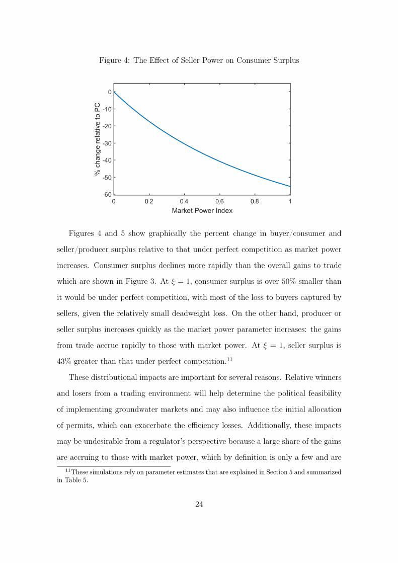
Figure 4: The Effect of Seller Power on Consumer Surplus
Figures 4 and 5 show graphically the percent change in buyer/consumer and
seller/producer surplus relative to that under perfect competition as market power
increases. Consumer surplus declines more rapidly than the overall gains to trade
which are shown in Figure 3. At ξ = 1, consumer surplus is over 50% smaller than
it would be under perfect competition, with most of the loss to buyers captured by
sellers, given the relatively small deadweight loss. On the other hand, producer or
seller surplus increases quickly as the market power parameter increases: the gains
from trade accrue rapidly to those with market power. At ξ = 1, seller surplus is
43% greater than that under perfect competition.11
These distributional impacts are important for several reasons. Relative winners
and losers from a trading environment will help determine the political feasibility
of implementing groundwater markets and may also influence the initial allocation
of permits, which can exacerbate the efficiency losses. Additionally, these impacts
may be undesirable from a regulator’s perspective because a large share of the gains
are accruing to those with market power, which by definition is only a few and are11These simulations rely on parameter estimates that are explained in Section 5 and summarized
in Table 5.
24

Figure 5: The Effect of Seller Power on Producer Surplus
likely to be large agribusiness enterprises with significant landholdings.
4.2.3 Buyer Market Power
In the same way, we can alternatively introduce buyer market power (ξ = 0, θ > 0)
into the framework. In this case, the buyers act as if they are facing a perceived
marginal factor cost curve, which results in an equilibrium with less trade and a
lower price. The perceived marginal factor cost curve is a linear combination of the
monopsony marginal factor cost curve (MFC(XTL )) and the market inverse supply
curve (ES(XTL )) with weights given by the oligopsony power parameter, θ:
PMFC(XTL ) = θMFC(XT
L ) + (1−θ)ES(XTL ) =
2
η(2δXT
L − δX0L−
α(1 + η)
1 + α), (32)
where the marginal factor cost is given by MFC(XTL ) = 2
η(2δXT
L − δX0L −
α(1+η)1+α
).
Equilibrium quantity, denoted XTBP , is determined by the intersection of the per-
ceived marginal factor cost curve and the buyers’ excess demand. Permit price, ρBP ,
25
is determined where XTBP intersects the excess supply curve:
XTBP =1
δ
Ω
2 + θ= (
2
2 + θ)XT ∗
, (33)
ρBP =2
η(α(1 + η)
1 + α− δX0
L +Ω
2 + θ) = ρ∗ + (
2
2 + θ− 1)
Ω
η. (34)
Equations (33) and (34) show that buyer power will depress trade in the water
market and reduce price relative to the competitive equilibrium. By taking the
derivative with respect to the market power parameter, we can see how seller market
power affects market outcomes:
∂XTBP
∂θ= −1
δ
Ω
(2 + θ)2< 0
∂ρBP
∂θ= −2
η
Ω
(2 + θ)2< 0 (35)
The solutions to the buyer market power case are symmetric to the seller power
scenario. In either case, a larger market power parameter implies fewer permits
traded and thus efficiency loss relative to the competitive equilibrium. As one would
expect, the price is higher than the competitive counterpart when there is seller
power, and lower in the presence of buyer power. Both sets of solutions depend on
the demand elasticity and other parameters from the profit maximization problems.
5 Application to Coachella Valley, California
We now turn to estimating the magnitude of the gains to trade relative to command
and control for a particular irrigation district. The Coachella Valley, CA is an
ideal setting for an application of the model because it is both subject to mandates
under SGMA and home to large grower-shippers that may dominate the market for
permits if trading occurs in the future. A novel feature of this application is that all
26

the model parameters are either constructed or estimated using observational data
from this area. Micro-level panel data on groundwater extraction and price from the
Coachella Valley Water District allow me to generate a well-identified price elasticity
estimate. With estimates of the groundwater demand elasticity, the demand shift
parameter, and the efficiency parameter that are reflective of a real-world setting,
I quantify the gains to trade and express the benefits relative to surplus under
command and control.
5.1 Background
The Coachella Valley is a productive agricultural region in southern California that
depends partly on groundwater for irrigation and is subject to restrictions under
SGMA. It has roughly 65,000 acres in crop production with a total production value
of over half a billion dollars a year. Producing 95% of the nation’s dates, the area is
also well-known for the production of table grapes, citrus fruits, bell peppers, and
other vegetables. Identified in Figure 6, it is located in Riverside County just north
of the Salton Sea and southeast of the San Bernardino Mountains.
Receiving only about 4 inches of precipitation in an average year, agriculture in
the area depends on both groundwater and imported Colorado River water for irri-
gation. The Coachella Valley groundwater basin has suffered at times from ground-
water overdraft, the condition wherein pumping exceeds groundwater recharge over
a period of years. As a result, three of the Valley’s four groundwater subbasins
have been classified as “medium priority” by the California Department of Water
Resources, which means the local agencies are subject to a timeline and set of goals
mandated by SGMA for reaching groundwater sustainability. However, relative to
the “high priority” basins in the state, this area does not face overdraft conditions
as severe as some others.
The Coachella Valley Water District (CVWD), the largest water agency in the
27
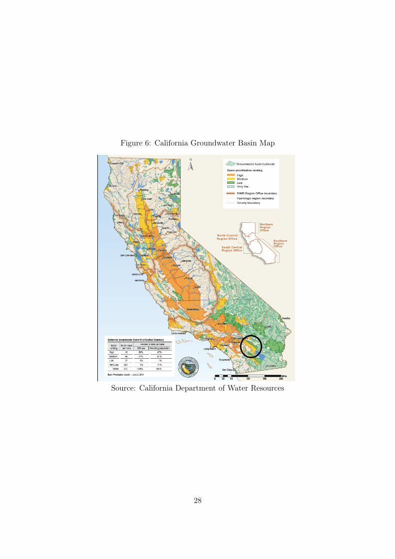
Figure 6: California Groundwater Basin Map
Source: California Department of Water Resources
28

Figure 7: Replenishment Assessment Charge (RAC) by Region
Coachella Valley, is unique in that it charges location-specific volumetric prices to
groundwater users for pumping. CVWD imports Colorado River water to artificially
replenish the aquifer in three locations throughout its service area, and charges sep-
arate prices to groundwater users within those three areas to fund the replenishment
program. The three geographic regions, East Whitewater, West Whitewater, and
Mission Creek, share some common features. Within each region, all customers face
a uniform price per acre-foot for groundwater extraction, called the Replenishment
Assessment Charge (RAC). When rate changes occur, they happen in the same
month of the year for all regions facing a rate increase. The regions differ in some
important ways as well; both the groundwater extraction fee and the level of price
increases vary substantially across regions. We exploit this plausibly exogenous vari-
ation in prices across space and time to estimate the price elasticity of groundwater
demand for the Coachella Valley.
Figure 7 shows the variation in extraction prices across time and region. The
RAC for the West Whitewater region began prior to 2000, so users in that area have
29

a nonzero groundwater price throughout our sample set. All other rate increases
occurred during July of each year. The East Whitewater region faces the lowest
RAC, remaining below $50/AF through June 2014. Prices vary only at the region-
year level. Figure 7 showcases the variability in the price changes across regions,
e.g., periods of time when rates changed for the East Whitewater region, but not
the others.
Most of the groundwater users in the CVWD service area have access to surface
water in addition to groundwater. Surface water from the Colorado River is deliv-
ered to CVWD customers and to the groundwater replenishment facilities via the
Coachella Canal. Unlike the RAC, canal rates vary by usage category (agricultural,
municipal, etc.) and not by region. Surface water is delivered periodically to the
groundwater replenishment facilities for recharge at the sites and these delivered
water quantities vary due to drought conditions and other factors.
Groundwater use in the Coachella Valley spans agricultural, urban, and recre-
ational uses. RAC program data are not collected by usage category, so CVWD is
unable to segregate agricultural wells from municipal wells, golf wells, etc. As of
2005, 45% of water use came from the agricultural sector, 33% of water use came
from urban (residential and industrial) users, and 17% of water was used by golf
courses (Coachella Valley Water District, 2012). Data are not available on how this
make-up has changed from 2000 to 2016, or how it varies among regions.
5.2 Price Elasticity of Demand for Groundwater
The price elasticity of demand for groundwater is not only an important parameter in
estimating the gains from trade, but it is also a necessary statistic in understanding
the potential of price as a lever to manage groundwater demand. The deployment
of three different pricing regimes for groundwater extraction within the Coachella
Valley provides an opportunity to estimate the effect of prices on groundwater use. I
30

take advantage of monthly, well-level data spanning 17 years to estimate the effect of
a uniform, volumetric pumping fee on well-level groundwater extraction, controlling
for well fixed effects, month aggregate shocks, and other potentially confounding
factors. I find the groundwater demand to be highly inelastic, with an estimate of
-0.19. To my knowledge, this provides the first micro-level estimate of the price
elasticity of groundwater demand that does not rely on estimates of pumping cost
for price. In what follows, I introduce the data, explain the empirical strategy, and
present estimation results.
5.2.1 Data
The dataset is an unbalanced panel that spans 17 years and over 900 individual
wells overlying the Coachella Valley Groundwater Basin. Received directly from
the Coachella Valley Water district, the dataset includes groundwater extraction
per month of every well in the RAC program from 2000 to 2016.12 Although the
RAC program for the West Whitewater region began prior to 2000, this is not the
case for the other two regions. The Mission Creek and East Whitewater regions
began facing groundwater fees in July 2004 and January 2005, respectively. The
unbalanced panel reflects the addition of new wells to the program over time.
Monthly groundwater extraction varies across seasons and regions. Average ex-
traction may vary by region because of differences in land use, the RAC, availability
of surface water, and other factors. The West Whitewater region has both the high-
est average extraction and the highest average RAC across the three regions whereas
the East Whitewater region has the lowest average extraction and lowest average
price. Figure 8 displays average monthly groundwater extraction by region over
time. The vertical line depicts when the RAC was introduced. Figure 8 shows the12The RAC program includes all groundwater wells that extract more than 25 acre feet in a
year. Extraction must be reported to CVWD on a monthly basis and is subject to the RAC of theregion in which the well is located.
31

Figure 8: Average Monthly Groundwater Extraction by Region
32

clear seasonal fluctuations associated with groundwater extraction.
Table 1 provides descriptive statistics of all the variables in the dataset, which in-
clude other factors that impact groundwater use and may be correlated with ground-
water prices. In addition to well-level groundwater extraction, historical price (RAC)
data were received directly from the Coachella Valley Water District.
Table 1: Descriptive Statistics
Mean Std Dev Min MaxMonthly Groundwater Extraction (AF) 58.12 67.93 0.00 537.10Replenishment Assesment Charge ($/AF) 64.40 34.22 0.00 128.80Monthly Cummulative Precip (Inches) 0.19 0.26 0.00 1.76Monthly Average of Max Daily Temp (F) 89.21 13.29 67.84 111.29Monthly Average of Min Daily Temp (F) 61.24 13.13 40.68 84.71Growing Degree Days (8-32C) 6.23 1.26 3.38 7.44Harmful Degree Days (over 34C) 4.15 4.46 0.00 11.18Annual Recharge to Facilities (Hund. Thous. AF) 0.53 0.70 0.00 2.57Monthly Surface Water Use (Hund. Thous. AF) 0.27 0.07 0.08 0.40Annual Recycled Water Use (Thous. AF) 0.35 0.42 0.00 1.72Annual State Water Project Allocation (%) 53.93 26.64 5.00 100Drought Index: None (%) 25.87 38.44 0.00 100.00Drought Index: D0 (%) 17.59 22.65 0.00 97.94Drought Index: D1 (%) 23.40 25.32 0.00 100.00Drought Index: D2 (%) 22.88 27.35 0.00 100.00Drought Index: D3 (%) 10.18 21.41 0.00 100.00Drought Index: D4 (%) 0.07 0.13 0.00 0.41Proportion Citrus (%) 15.51 2.53 12.56 21.64Proportion Tree, Vine (%) 27.45 2.18 24.84 33.89Proportion Vegetable, Melon, Misc. (%) 46.56 4.07 34.59 50.81Proportion Field, Seed (%) 4.06 0.91 1.30 5.01Proportion Nursery (%) 6.42 1.32 4.53 9.63Area Irrigated (Acres) 54807 3733 43613 59626Observations 65108Note: Drought indices give the percentage of land in Riverside County experiencing differentdegrees of dryness from D0 representing "abnormally dry" conditions up to D4 representing "ex-ceptional drought" conditions.
Data on drought and aggregate weather shocks were obtained to account for
ways in which these factors may affect groundwater extraction and prices over time.
Daily precipitation and temperature data were collected from a weather station at
33

the Indio Fire Station (National Climatic Data Center #4259) in Riverside county.
Daily precipitation data were summed to aggregate to the monthly level. Growing
degree day and harmful degree day variables were constructed from daily average
temperatures and used in place of temperature.13 The California Department of
Water Resource’s State Water Project allocation announcements, which range from
0-100% of quantities requested in State Water Project surface water contracts, may
represent aggregate shocks that influence the amount of water available to ground-
water replenishment facilities within CVWD’s service area. Lastly, monthly values
of the U.S. Drought Monitor Index for Riverside County were collected over the
relevant time period (U.S. Department of Agriculture, 2017). D0 represents the
percentage of land in Riverside County facing "abnormally dry" conditions in a
given year. D4 is the most extreme degree of drought, representing conditions of
"exceptional drought". All are expressed as a percentage of land coverage in that
category.
Data on the availability of alternative water supplies were also obtained to ac-
count for the possibility of these factors affecting both prices and groundwater ex-
traction. Surface water is used for both direct consumption at the farm level and for
groundwater recharge across the regional groundwater replenishment facilities. The
amount of water delivered to groundwater replenishment facilities for the sake of
recharging the aquifer was reported in documents produced by the Coachella Valley
Water District (CVWD, 2016). Monthly consumptive use of surface water diverted
from the Colorado River for direct use is reported by the Bureau of Reclamation and
represents surface water use on behalf of all users in the service area of the Coachella13Agronomists model temperature by converting daily temperatures to growing degree days,
a nonlinear transformation of temperature that more accurately reflects the way crops respondto heat. Growing degree days are derived by summing the degrees above a lower baseline andbelow an upper threshold during the growing season. Following Richie and NeSmith (1991) andSchlenker, Hanemann, and Fisher (2007), we use the range from 8C to 32C, within which plantgrowth is assumed to be linear. Days with temperatures above 34C, assumed to be harmful toplant growth, are used to construct harmful degree days.
34

Valley Water District (U.S. Department of Interior, 2017). Furthermore, users in
two regions receive limited recycled water to be used in-lieu of groundwater. Data
on recycled water deliveries by region were collected from documents published by
the Coachella Valley Water District (CVWD, 2016).
5.2.2 Empirical Strategy
To estimate the price elasticity of demand for groundwater in the Coachella Valley, I
take advantage of substantial variation in groundwater prices across regions and time
within the water district’s service area. I use panel data on groundwater extraction
and replenishment charges (RAC) spanning 17 years to estimate a fixed effects model
using ordinary least squares.
The basic estimating equation is
ln(wit) = αi + βln(RACit) +D′mδ +X ′itγ + εit, (36)
where the dependent variable, ln(wit), is the natural log of groundwater extraction
for well i in month t. The parameter of interest β is the coefficient on the natural
log of groundwater prices, denoted ln(RACit). Equation (36) includes a vector
of control variables, represented by Xit, which includes precipitation, degree days,
State Water Project (SWP) allocations, and surface water quantities for both direct
consumption and recharge at the replenishment facilities. Well-specific fixed effects,
αi, allow flexibility in capturing differences across wells; this controls for all well
characteristics possibly correlated with RAC that are unchanged over time, i.e.,
differences in soils or other hydrogeologic features. The variable Dm is a set of
monthly dummy variables that allows us to net out seasonal fluctuations in pumping.
Lastly, εit is an idiosyncratic error term. Standard errors are clustered at the well
level to allow for serial correlation within a well over time.
35

Because the RAC changes annually and prices have increased over time, annual
fixed effects soak up substantial variation in price changes. For this reason, I in-
tentionally omit year and month-year fixed effects in this empirical approach, and
instead explicitly account for relevant aggregate (basin-wide) shocks and region-
varying shocks by conditioning on time-varying observables. To account for the fact
that drought and weather may affect both groundwater use and prices, I control for
precipitation, degree days, and the percentage of land in Riverside county facing
different levels of drought. Since some of CVWD’s water for recharge at the ground-
water replenishment facilities comes from the State Water Project, I also condition
on annual SWP water project allocations. Furthermore, since regional differences
in prices are partially driven by the amount of water recharged at replenishment
facilities over time, I include regional groundwater recharge as a control variable,
thus capturing relevant time-varying, regional shocks.
For the coefficient of interest β to capture the causal effect of price changes
on groundwater use, no region-level time-varying unobservables that affect extrac-
tion can be systematically correlated with prices. While it cannot be demonstrated
that this identifying assumption holds, I empirically examine its plausibility in what
follows. Threats to identification of β in equation (36) come from region-level time-
varying omitted variables that are both correlated with RAC and influence ground-
water extraction. Identification of the impact of price on extraction comes from
variation in the RAC across regions and time, while controlling for time-invariant
well characteristics, aggregate shocks, and other confounding factors.
The inclusion of surface water variables, one for direct consumption and the
other for groundwater recharge at regional replenishment facilities, is motivated
by features of our institutional setting. Surface water availability and use may be
correlated with both groundwater prices and groundwater extraction. Given a fixed
annual allocation of Colorado River water, the amount of groundwater extracted, the
36

quantity surface water applied, and the water remaining for groundwater recharge
within the basin are likely correlated. The RAC is largely determined by replenish-
ment program costs, which is a function of the amount of water used for recharge at
the various groundwater replenishment facilities. By including both surface water for
direct consumption and surface water for recharge at the facilities (which varies by
region) as control variables in the specification, we eliminate these potential threats
to identification.
Changes in energy prices may confound the estimation of β since energy prices
may be correlated with the RAC and likely affect groundwater extraction; pumping
costs are partially determined by the energy requirements to lift the groundwater
from below. In our empirical setting, a single utility supplies energy and all users
face the same rates and rate changes. The region faced virtually no rate changes over
the relevant time period. Imperial Irrigation District, the main energy provider for
Coachella Valley groundwater pumpers, did not change electricity rates from 2000 to
2014 and only increased them by $0.03 per kWh for 2015 and 2016. Furthermore, we
need not worry about differences in energy costs across individuals that are driven
by differences in pressure or depth to the water table because this is not likely
correlated with the agency-determined RAC.
Differences in land use across region and time may also pose a threat to iden-
tification because land use affects groundwater extraction and may be correlated
with the RAC. Groundwater wells in this dataset span agricultural and municipal
uses, and a portion of wells irrigate grasses on golf courses. The East Whitewater
region is predominantly agricultural, and this could potentially affect the replenish-
ment activities of the facility in the area, correlating land use with the RAC. These
characteristics are only problematic if they influence the replenishment charge in
that region. Coachella Valley Water District Engineering Reports, which justify
RAC rate changes, show no evidence of correlation between the RAC and land use
37

(CVWD, 2016).
Differences in hydrogeology that coincide with the rate zones may affect both
pumping decisions and the costs at respective replenishment facilities, possibly con-
founding the estimation of β. The three areas differ in proximity to the Salton Sea,
and thus may vary in groundwater quality. Distance to the Salton Sea, soil type, and
other natural features are time-invariant and thus captured with well fixed effects.
5.2.3 Results
Results from the estimation of equation (36) are reported in Table 2. Column (1)
reports results from an OLS regression of the log of groundwater extraction on
the log of prices controlling for well fixed effects. Column (2) further controls for
month fixed effects and column (3) controls for aggregate shocks by conditioning on
basin-wide surface water consumption, drought, precipitation, squared precipitation,
degree days, and SWP allocations. Column (4) further conditions on region-level,
time-varying observables, namely, delivered water for recharge at the regional re-
plenishment facilities.
With a price elasticity point estimate of -.19 in the preferred specification of col-
umn (4), results suggest that prices impact extraction in a modest, yet statistically
significant way. If the price of groundwater is increased by 1%, we expect this to
cause a decrease in extraction of 0.19%. Results from Table 2 show the robust-
ness of results to the inclusion of controls for seasonal effects, aggregate shocks, and
groundwater recharge.
Table 3 presents the robustness of the baseline results to the inclusion of ad-
ditional control variables for other potentially relevant factors. Also, to check the
sensitivity to assumptions on functional form, Table 3 includes results for the OLS
regression of groundwater extraction on prices in levels, controlling for well and
month fixed effects, aggregate shocks, and groundwater recharge. As a basis for com-
38
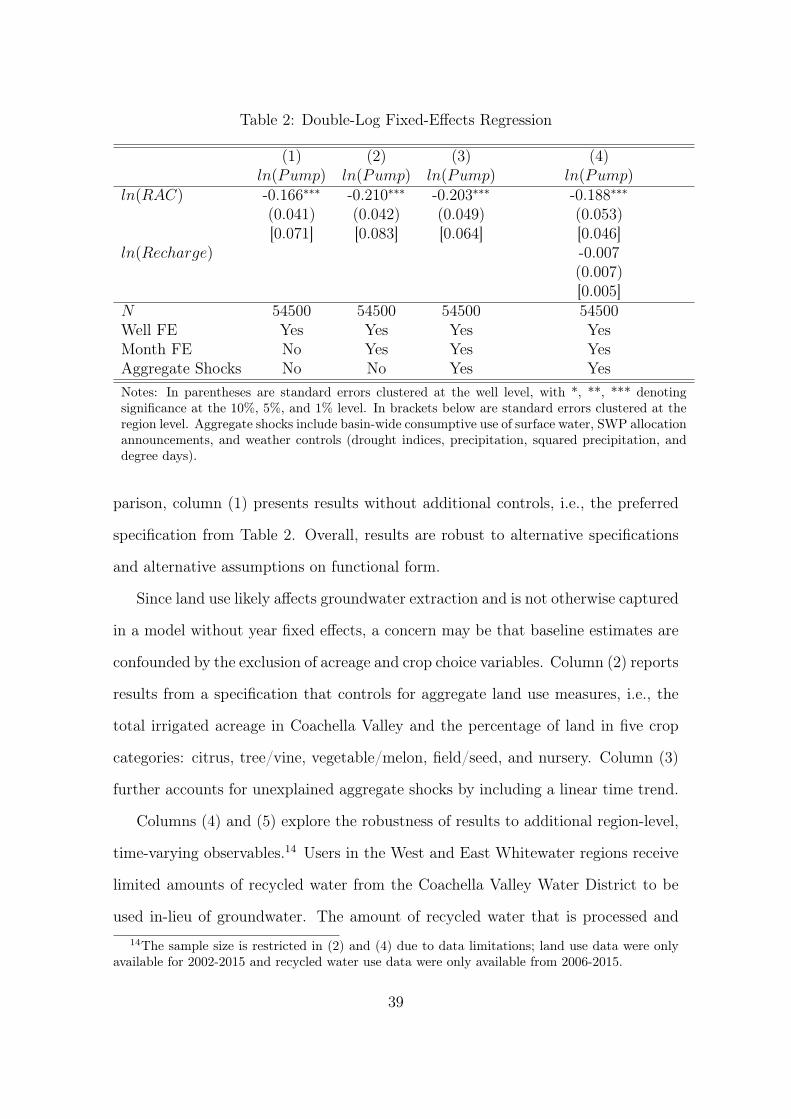
Table 2: Double-Log Fixed-Effects Regression
(1) (2) (3) (4)ln(Pump) ln(Pump) ln(Pump) ln(Pump)
ln(RAC) -0.166∗∗∗ -0.210∗∗∗ -0.203∗∗∗ -0.188∗∗∗(0.041) (0.042) (0.049) (0.053)[0.071] [0.083] [0.064] [0.046]
ln(Recharge) -0.007(0.007)[0.005]
N 54500 54500 54500 54500Well FE Yes Yes Yes YesMonth FE No Yes Yes YesAggregate Shocks No No Yes YesNotes: In parentheses are standard errors clustered at the well level, with *, **, *** denotingsignificance at the 10%, 5%, and 1% level. In brackets below are standard errors clustered at theregion level. Aggregate shocks include basin-wide consumptive use of surface water, SWP allocationannouncements, and weather controls (drought indices, precipitation, squared precipitation, anddegree days).
parison, column (1) presents results without additional controls, i.e., the preferred
specification from Table 2. Overall, results are robust to alternative specifications
and alternative assumptions on functional form.
Since land use likely affects groundwater extraction and is not otherwise captured
in a model without year fixed effects, a concern may be that baseline estimates are
confounded by the exclusion of acreage and crop choice variables. Column (2) reports
results from a specification that controls for aggregate land use measures, i.e., the
total irrigated acreage in Coachella Valley and the percentage of land in five crop
categories: citrus, tree/vine, vegetable/melon, field/seed, and nursery. Column (3)
further accounts for unexplained aggregate shocks by including a linear time trend.
Columns (4) and (5) explore the robustness of results to additional region-level,
time-varying observables.14 Users in the West and East Whitewater regions receive
limited amounts of recycled water from the Coachella Valley Water District to be
used in-lieu of groundwater. The amount of recycled water that is processed and14The sample size is restricted in (2) and (4) due to data limitations; land use data were only
available for 2002-2015 and recycled water use data were only available from 2006-2015.
39

Table3:
Rob
ustnessto
Alterna
tive
Specification
s
Add
itiona
lCon
trolsfor
(1)
(2)
(3)
(4)
(5)
(6)
(7)
Baseline
Land
Use
Tim
eTr
end
RecycledWater
Lagged
Prices
AgRegionOnly
Levels
ln(RAC
)-0.188∗∗∗
-0.136∗∗
-0.118∗
-0.173∗∗∗
-0.175∗∗∗
-0.201∗∗∗
(0.053
)(0.069
)(0.062
)(0.064
)(0.061
)(0.078
)[0.046
][0.025]
[0.014
][0.007
][0.038
]RAC
-0.255∗∗∗
(0.064
)[0.065
]N
5450
050
533
5450
04173
853
924
2266
354
933
WellF
EYes
Yes
Yes
Yes
Yes
Yes
Yes
Mon
thFE
Yes
Yes
Yes
Yes
Yes
Yes
Yes
Agg
rega
teSh
ocks
Yes
Yes
Yes
Yes
Yes
Yes
Yes
Notes:The
baselin
especification
correspo
ndsto
thepreferredspecification
ofcolumn(4)in
Tab
le2.
Eachsubsequent
columnrepo
rtsan
alternate
specification
.W
iththeexceptionof
column(7),
which
provides
estimates
oftheOLS
regression
inlevels,thedepe
ndentvariab
leis
thelogof
grou
ndwater
extraction
.Stan
dard
errors
clusteredat
thewelllevel
arerepo
rted
inpa
rentheses,with*,
**,*
**deno
ting
sign
ificanceat
the10%,5
%,
and1%
level.Stan
dard
errors
clusteredat
theregion
levela
rerepo
rted
belowin
brackets.Aggregate
shocks
includ
eba
sin-wide,mon
thly
consum
ptive
useof
surfacewater,a
nnua
lSW
Pallocation
anno
uncements,a
ndweather
controls(droug
htindices,precipitation,
squa
redprecipitation,
anddegree
days).
40

delivered within a year affects the agency’s costs, and thus may influence the RAC,
and may also impact well-level groundwater extraction. Column (5) includes a one
year lag of RAC prices to account for the possibility that groundwater pumpers may
be slow to adjust to price changes. The insensitivity of the elasticity estimate to the
inclusion of additional controls demonstrates the robustness of the estimate.
Since the East Whitewater region is predominantly agricultural, I report results
in column (6) from a restricted sample of wells in the East Whitewater region only.
Although we do not know which individual wells within this dataset are pumping
groundwater for agricultural purposes, I proxy for this by focusing on the region
that is primarily agricultural. Results show a slightly more elastic estimate when
focusing on this region alone.
Column (6) presents results from an OLS regression of groundwater extraction
on RAC in levels, controlling for well and month fixed effects, aggregate shocks, and
groundwater recharge. The coefficient estimate of -0.25 in column (7) translates to
a demand elasticity point estimate of -.28, when evaluating at the mean values for
extraction and RAC. Since the gains from trade are increasing in the price elasticity
of demand, my use of the -.19 estimate from the double-log specification provides a
conservative, lower bound in the following analysis.
5.3 Other Simulation Model Parameters
The remaining parameters for the simulation model were also estimated with data
from the Coachella Valley. First, the demand shift parameter α, which is the ratio
of marginal value products between low- and high-value crops at any quantity of
groundwater, was calculated with data from Riverside County’s 2015 Crop Report
for Coachella Valley and University of California Cooperative Extension (UCCE)
Cost and Return Studies. For simplicity, we focus on the four leading crops (grapes,
lemons, bell peppers, and dates), which are listed with production value and acreage
41

Table 4: Top Four Crops Grown in the Coachella Valley, CA
Crop Revenue Acreage Revenue ValuePer Acre Type
Grapes $131,852,825 7,802 $16,900 HighLemon/lime $93,824,406 3,887 $24,138 HighBell Peppers $87,891,750 4,490 $19,575 HighDates $36,184,900 7,765 $4,660 Low
in Table 4.
To estimate α, I first estimated a point on the value marginal product curve of
water for each crop. UCCE Cost and Return Studies report applied water per acre
by crop and Riverside County’s Crop Report discloses production and value per acre
by crop. Used together, a point on the average product curve of water by crop was
identified by dividing average production by applied water per acre. As shown in
Appendix A, economic theory can then be applied to relate this point to a point on
the value marginal product curve.
With the per-acre value reported in Riverside County’s 2015 Crop Report for
Coachella Valley, I derived a point on the marginal revenue product curve, extrap-
olated to the intercept with an elasticity estimate, and compared across crops. In
this fashion, the demand shift index can be computed for any pair of crops. For the
purposes of this simulation, I needed to arrive at a single alpha; the estimate of α is
given by the ratio of the intercepts between H- and L-type groundwater demands. I
used dates as the low-value crop and generated a high-value crop bundle consisting
of table grapes, lemons, and bell peppers.
Another model parameter, the total endowment of pumping rights, X0H + X0
L,
was estimated to be 80% of Coachella’s “business as usual” groundwater extraction,
meaning a 20% reduction in water use to correct for basin overdraft. This was
calculated by comparing the average annual groundwater extraction in Coachella to
that which would be allowed on the basin if it were to eliminate its reported 70,000
42

Table 5: Parameter Estimates
Parameter Estimate SourceDemand Shift Index .1 Estimated by comparing intercepts of H(0 < α < 1) tand L type water demands, which were
proxied with estimates of water demandsfor Coachella’s four leading crops.
Demand Elasticity (η) -.19 Estimated with fixed effects regressionsusing well-level pumping and price datafrom CVWD.
Total Allowable .8 Calculated by comparing average annualExtraction (X0
L +X0H) basin total pumping with CVWD’s
annual overdraft estimates.Irrigation Efficiency (δ) .85 Rogers et al. (1997)
AF/year of groundwater overdraft (Coachella Valley Water District, 2016). Lastly,
an irrigation efficiency of 85% was chosen for δ because this is the reported average
distribution efficiency for drip technology. Drip technology is used by growers of
grapes, lemons, and bell peppers in the Coachella Valley (Rogers et al., 1997). An
irrigation efficiency of 85% is also the distribution efficiency used in UCCE Cost
and Return Studies for drip irrigation systems (O’Connell et al., 2015). All model
parameters for Coachella Valley are summarized in Table 5.
5.4 Results for Coachella Valley, California
Using the parameter estimates summarized in Table 5, I estimate the magnitude of
the gains from groundwater trade for the Coachella Valley. Recall that the expres-
sions derived in Section 3 reflect only the case when permit allocations are binding
for both types. At the parameter values estimated for the Coachella Valley, how-
ever, the constraint is not binding for the L types. Results reported here reflect the
discontinuity associated with a kinked supply curve that results from an allocation
that binds for the H types only.15
15In this case, the inverse excess supply curve ES(XT ) = 0 up until the point where the Ltypes are willing to sell at a positive price; this point is denoted x = X0
L − 1δ (α(1+η)1+α ) in equation
43

Equation (37) reports an expression for the percent change in surplus from al-
lowing trade relative to a command-and-control scenario when the L types are not
constrained. Using this expression and our estimates of the model parameters, I show
that the gains from trade are large for two different allocation scenarios. The two sce-
narios considered are: (1) an equal allocation between types (X0L = X0
H = .4) and (2)
an unequal allocation that is proportional to acreage shares (X0L = .26, X0
H = .54).16
For an equal allocation between types, the percent change in surplus relative to
command and control is
%4 = ∫ x0ED(τ)dτ +
∫ Ω2δ
x(ED(τ)− ES(τ))dτ∫ X0
H
0xH(τ)dτ −X0
H [2δη
(1δ( 1+η
1+α)−X0
H)] +∫ x
0xL(τ)dτ − x
∗ 100 = 427% (37)
where x = X0L− 1
δ(α(1+η)
1+α) and x = α( 1+η
1+α)− η
2. Thus, surplus with trade is over five
times greater than the benefits under a no-trade scenario.
The value of the gains from trade for the Coachella Valley in this case can be
calculated, given estimates of both aggregate annual groundwater extraction and the
full per-unit pumping price. An irrigator’s full price per acre-foot of groundwater is
equal to the RAC plus the energy cost to pump an acre-foot of water to the surface.
Using an average depth to water from the land surface of 152 feet and the local
energy provider’s $.0618/kWh energy price for agricultural uses in 2016, I apply an
engineering formula from Rogers and Alam (2006) to calculate the average per-unit
energy cost of extraction. With an approximate (full) groundwater price of $99/AF
and an aggregate annual groundwater extraction of 464,400 AF, the gains from trade
are approximately $119 million annually.
(37). Thus, we have a kinked supply curve and a quadrilateral-shaped gains area. Furthermore, anon-binding constraint for the L types affects the surplus calculation under the baseline command-and-control scenario, which alters the denominator of equation (37).
16This allocation was calculated with acreage values from Table 4, scaled to reflect the totalallowable extraction of 80% of “business as usual” pumping.
44

Given California’s legal history, an allocation of permits that is proportional
to land holdings is a more likely scenario. For an allocation of permits based on
acreage, the percent change in surplus relative to command and control is
%4 = 144%. (38)
Surplus with trade is over twice as large in this case. With an approximate ground-
water price of $99/AF and an aggregate annual groundwater extraction of 464,400
AF, the annual gains from trade for the Coachella Valley in this case are approx-
imately $73 million. Since the L types receive fewer permits in this scenario, the
gains from trade are smaller than if permits were allocated equally between types.
Magnitudes generated with base Coachella values represent possible gains to
Coachella Valley groundwater users from water trading, if the water district imposed
pumping restrictions of a reasonable magnitude and distributed permits for pumping
in one of these ways. Given the model assumptions and parameter estimates of
Table 5, the gains from trade are large. These estimates suggest that, given a 20%
reduction in pumping from the status quo, surplus is at least twice as large with
trade than without.
Since we have no information on the magnitude of potential market power in this
area, these gains are calculated assuming a perfectly competitive permit market.
However, from analysis in Section 4, we know the gains from trade can be reduced
by at most 11% when ξ = 1, θ = 0 or θ = 1, ξ = 0, regardless of the initial allocation
of permits. The efficiency gains of groundwater markets relative to command and
control remain large even in the presence of market power. Thus, market power
should not be used as a possible argument against the formation of groundwater
markets. Even in the presence of monopoly power or monopsony power, efficiency
gains of markets relative to command and control are substantial.
45
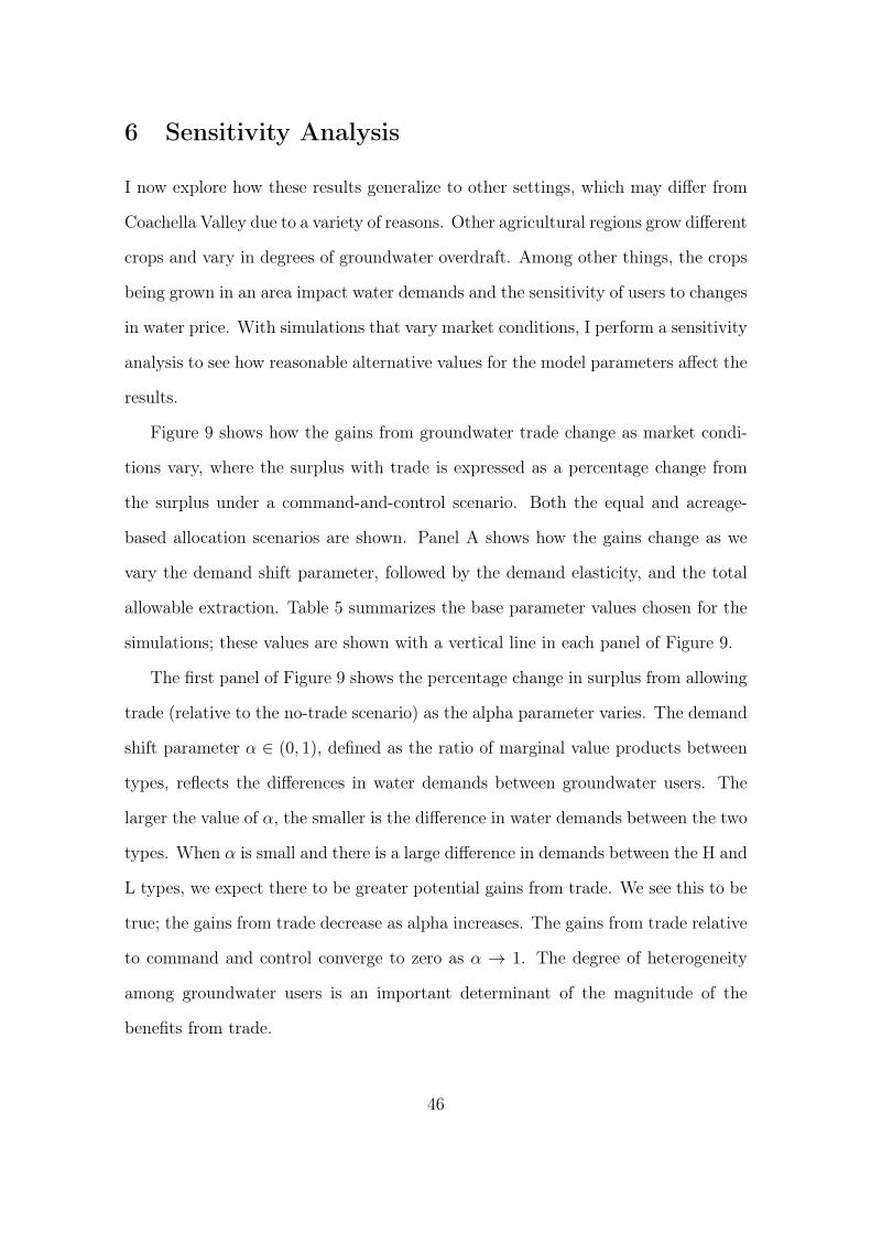
6 Sensitivity Analysis
I now explore how these results generalize to other settings, which may differ from
Coachella Valley due to a variety of reasons. Other agricultural regions grow different
crops and vary in degrees of groundwater overdraft. Among other things, the crops
being grown in an area impact water demands and the sensitivity of users to changes
in water price. With simulations that vary market conditions, I perform a sensitivity
analysis to see how reasonable alternative values for the model parameters affect the
results.
Figure 9 shows how the gains from groundwater trade change as market condi-
tions vary, where the surplus with trade is expressed as a percentage change from
the surplus under a command-and-control scenario. Both the equal and acreage-
based allocation scenarios are shown. Panel A shows how the gains change as we
vary the demand shift parameter, followed by the demand elasticity, and the total
allowable extraction. Table 5 summarizes the base parameter values chosen for the
simulations; these values are shown with a vertical line in each panel of Figure 9.
The first panel of Figure 9 shows the percentage change in surplus from allowing
trade (relative to the no-trade scenario) as the alpha parameter varies. The demand
shift parameter α ∈ (0, 1), defined as the ratio of marginal value products between
types, reflects the differences in water demands between groundwater users. The
larger the value of α, the smaller is the difference in water demands between the two
types. When α is small and there is a large difference in demands between the H and
L types, we expect there to be greater potential gains from trade. We see this to be
true; the gains from trade decrease as alpha increases. The gains from trade relative
to command and control converge to zero as α → 1. The degree of heterogeneity
among groundwater users is an important determinant of the magnitude of the
benefits from trade.
46

Figure 9: Gains from Trade Sensitivity Analysis
47
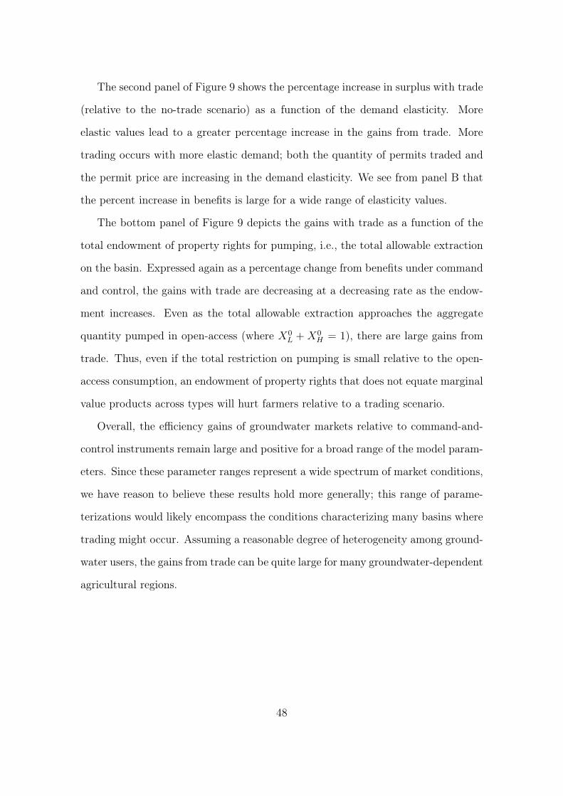
The second panel of Figure 9 shows the percentage increase in surplus with trade
(relative to the no-trade scenario) as a function of the demand elasticity. More
elastic values lead to a greater percentage increase in the gains from trade. More
trading occurs with more elastic demand; both the quantity of permits traded and
the permit price are increasing in the demand elasticity. We see from panel B that
the percent increase in benefits is large for a wide range of elasticity values.
The bottom panel of Figure 9 depicts the gains with trade as a function of the
total endowment of property rights for pumping, i.e., the total allowable extraction
on the basin. Expressed again as a percentage change from benefits under command
and control, the gains with trade are decreasing at a decreasing rate as the endow-
ment increases. Even as the total allowable extraction approaches the aggregate
quantity pumped in open-access (where X0L + X0
H = 1), there are large gains from
trade. Thus, even if the total restriction on pumping is small relative to the open-
access consumption, an endowment of property rights that does not equate marginal
value products across types will hurt farmers relative to a trading scenario.
Overall, the efficiency gains of groundwater markets relative to command-and-
control instruments remain large and positive for a broad range of the model param-
eters. Since these parameter ranges represent a wide spectrum of market conditions,
we have reason to believe these results hold more generally; this range of parame-
terizations would likely encompass the conditions characterizing many basins where
trading might occur. Assuming a reasonable degree of heterogeneity among ground-
water users, the gains from trade can be quite large for many groundwater-dependent
agricultural regions.
48

7 Conclusion
As regulators around the world strive for improved groundwater management, they
may consider market-based instruments to improve the allocation of limited water
resources. Prior to implementing a voluntary groundwater trading program, it is
important to understand how groundwater markets will function, how they might
be impacted by market power, and how market power influences other types of
behavior. This paper evaluates the potential for groundwater trading and sheds light
on the role for markets to manage water in the presence of imperfect competition.
I estimate the efficiency gains of groundwater markets relative to command-and-
control instruments in the presence of this market failure.
Imperfect competition may be an important characteristic of future groundwater
markets. When rights for use are allocated by land size or historical pumping in an
area characterized by large, vertically integrated farming operations, permits may
be concentrated in the hands of a few large players. Additionally, in areas where
trading occurs on the level of the water districts and agencies jointly governing a
basin, there is a small-numbers problem that will influence trading. To understand
the nature and magnitude of these impacts, the decisions of heterogeneous farmers to
buy or sell tradable water permits were modeled such that one side of the market has
a flexible degree of market power. I estimated the gains from trade in a real-world
setting and see how large of an issue market power can be.
Overall, I show that regardless of the degree of competition, there are significant
net benefits from a groundwater trading regime. With parameters estimated with
data from the Coachella Valley, I find that surplus with trade is over twice as large
as the surplus under command and control, assuming perfect competition. Given
that the gains can be reduced by at most 11% with market power on one side of
the market, we conclude that the gains remain large regardless of permit market
49

structure. Furthermore, I show that the gains remain large over a broad range of
parameterizations by showing the sensitivity to changes in the demand elasticity,
the endowment of property rights, and the demand shift index, which captures the
degree to which marginal value products differ between buyers and sellers. Thus,
although other groundwater basins will exhibit features that differ from Coachella
Valley, these results are likely to hold more broadly.
To evaluate the role of market power, I show both how the total gains from
trade decrease and how the distribution of benefits changes relative to the perfectly
competitive baseline. The reduction in the total gains from trade from any degree of
market imperfection is small. Considering the magnitude of the potential gains from
trade, this welfare loss should not be used as an argument against the formation of
groundwater markets. Groundwater users as a whole are still significantly better off
than under command and control. However, the distributional impacts of market
power can be large, socially undesirable, and a factor in the political economy of
implementing trading regimes. The majority of the gains from trade accrue to the
few with market power, which are likely large agribusiness enterprises.
The distributional impacts of market power provide insight into how groundwater
markets may develop. First, a groundwater trading regime will require considerable
political support among groundwater users. The distributional dimension of market
power may dissipate support from the group being subjected to the market power,
since much of this group’s potential gains from trading will be captured by those
with market power. However, the converse is true in that a group that thinks
it has market power in trading would be strongly supportive. Second, a trading
regime must be preceded by the allocation of property rights for pumping. Big
players may exert influence on the method of permit allocation prior to trading,
exacerbating the distributional impacts of market power. Although our results imply
that permits should be allocated to avoid their concentration in the hands of a few
50
buyers or sellers, this may be infeasible due to the political environment and/or
limited information on behalf of the regulator. There is room for additional work on
the interaction between different permit allocations and the exercise of market power,
with the goal of determining the best permit allocations given limited information.
References
[1] California Department of Water Resources. 2016. “California’s Groundwater:Working Toward Sustainability.” Bulletin 118 Interim Update 2016.
[2] Coachella Valley Water District. 2016. “Coachella Valley Water District Engi-neer’s Report on Water Supply and Replenishment Assessment for the MissionCreek Subbasin Area of Benefit, West Whitewater River Subbasin Area of Ben-efit, and East Whitewater River Subbasin Area of Benefit 2016-2017.”
[3] Coachella Valley Water District. 2012. “Coachella Valley Water ManagementPlan 2010 Update.”
[4] Faunt, C.C., K. Belitz, and R.T. Hanson. 2009. “Groundwater Availability inCalifornia’s Central Valley” in Groundwater Availability of the Central ValleyAquifer, California., ed. Claudia C. Faunt. Reston, VA: U.S. Geological Survey.
[5] Fowlie, M., S. Holland and E. Mansur. 2012. “What Do Emissions MarketsDeliver and to Whom? Evidence from Southern California’s NOx TradingProgram,” American Economic Review 102(2):1-29.
[6] Gonzalez-Alvarez, Y., A. Keeler, and J. Mullen. 2006. “Farm-Level Irrigationand the Marginal Cost of Water Use: Evidence from Georgia.” Journal of En-vironmental Management 80.4:311-317.
[7] Goulder, L.H., and I.H. Parry. 2008. “Instrument Choice in Environmental Pol-icy.” Review of Environmental Economics and Policy 2.2:307-322.
[8] Hahn, R.W. 1984. “Market Power and Transferable Property Rights.” TheQuarterly Journal of Economics 99.4:753-765.
[9] Hearne, R.R. and K.W. Easter. 1997. “The Economic and Financial Gains fromWater Markets in Chile.” Agricultural Economics 15:187-199.
[10] Hendricks, N.P., and J.M. Peterson. 2012.“Fixed Effects Estimation of the In-tensive and Extensive Margins of Irrigation Water Demand." Journal of Agri-cultural and Resource Economics 37.1:1-19.
51

[11] Kaiser, H.M., and N. Suzuki. 2006. New Empirical Industrial Organization andthe Food System. New York: Peter Lang Publishing, Inc.
[12] Kunkel, K.E., et al. 2013. "Monitoring and Understanding Trends in ExtremeStorms: State of Knowledge." Bulletin of the American Meteorological Society94.4:499-514.
[13] Mieno, T. and N. Brozovic. 2017. “Price Elasticity of Groundwater Demand:Attentuation and Amplification Bias due to Incomplete Information” AmericanJournal of Agricultural Economics 99.2:401-426.
[14] Misiolek, W.S., and H.W. Elder. 1989. “Exclusionary Manipulation of Marketsfor Pollution Rights.” Journal of Environmental Economics and Management16.2:156-166.
[15] Montero, J-P. 2009. “Market Power in Pollution Permit Markets.” The EnergyJournal 30.2:115-142.
[16] O’Connell, N.V., C.E. Kallsen, K.M. Klonsky, and K.P. Tumber. 2015. “SampleCosts to Establish an Orchard and Produce Lemons.” University of CaliforniaCooperative Extension Current Cost and Return Studies. University of Califor-nia Agricultural Issues Center.
[17] Perloff, J.M., L. Karp, and A. Golan. 2007. Estimating Market Power andStrategies. Cambridge: Cambridge University Press.
[18] Ritchie, J.T., and D.S. NeSmith. 1991. “Temperature and Crop Development”in Modeling Plant and Soil Systems, ed. John Hanks and J.T. Ritchie, 5-29.Madison: American Society of Agronomy.
[19] Riverside County Agricultural Commissioner’s Office. 2015. “Coachella ValleyAcreage and Agricultural Crop Report 2015.”
[20] Rodell, M., I. Velicogna, and J.S. Famiglietti. 2009 "Satellite-based Estimatesof Groundwater Depletion in India." Nature 460:999-1002.
[21] Rogers, D.H., F.R. Lamm, M. Alam, T.P. Trooien, G.A. Clark, P.L. Barnes,and K. Mankin. 1997. “Efficiencies and Water Losses of Irrigation Systems.”Irrigation Management Series MF-2243. Kansas State University.
[22] Rogers, D.H., and M. Alam. 2006. “Comparing Irrigation Energy Costs.” Irri-gation Management Series MF-2360. Kansas State University.
[23] Scheierling, S.M., J.B. Loomis, and R.A. Young. 2006. “Irrigation WaterDemand: A Meta-analysis of Price Elasticities.” Water Resources Research42:W01411.
52

[24] Schlenker, W., W.M. Hanemann, A.C. Fisher. 2007. “Water Availability, DegreeDays, and the Potential Impact of Climate Change on Irrigated Agriculture inCalifornia.” Climate Change 81.1:19-38.
[25] Suzuki, N., H.M. Kaiser, J.E. Lenz, K. Kobayashi, and O.D. Forker. 1994. “Eval-uating Generic Milk Promotion Effectiveness with an Imperfect CompetitionModel.”American Journal of Agricultural Economics 76.2:296-302.
[26] Takele, E., P. Mauk, and I. Sharabeen. 2005. “Sample Costs to Establish a DatePalm Orchard and Produce Dates in the Coachella Valley, Riverside County,2005-5006.” University of California Cooperative Extension Current Cost andReturn Studies. University of California Agricultural Issues Center.
[27] U.S. Department of Agriculture, 2017. “Percent Area in U.S. Drought MonitorCategories.”
[28] U.S. Department of the Interior, Bureau of Reclamation. 2017. “Colorado RiverAccounting and Water Use Report: Arizona, California, and Nevada.” CalendarYears 2000-2016.
[29] Vaux, H.J., and R.E. Howitt. 1984. “Managing Water Scarcity: An Evaluationof Interregional Transfers.” Water Resources Research 20.7:785-792.
[30] Westskog, H. 1996. “Market Power in a System of Tradeable C02 Quotas.” TheEnergy Journal 17.3:85-103.
[31] Zhang, M., and R.J. Sexton. 2002. “Optimal Commodity Promotion whenDownstream Markets Are Imperfectly Competitive.” American Journal of Agri-cultural Economics 84.2:352-365.
A Appendix: Deriving the Demand Shift Index
Assuming linear and declining value marginal products of water throughout, the
value marginal product curve will have twice the slope of the average revenue product
curve. Aggregate H-type and L-type demand curves both take the following form:
VMPx = a− bx. (A.1)
Thus, average revenue product curves are:
ARPx = a− b
2x (A.2)
53

By Equation A.1, we know the demand elasticity is:
|η| = 1
b
V MPxx
. (A.3)
Since we have an estimate of η and a point on the average revenue product curve, I
solve a system of three equations and three unknowns (a, b, VMPx) to find a point
on the value marginal product curve. Eliminating a and b, we can isolate VMPx,
VMPx =ARPx1 + 1
2η
(A.4)
The parameter of interest is the difference in marginal value products between types
at any x,
α = VMPH − VMPL =ARPH,x − ARPL,x
1 + 12η
(A.5)
The demand shift index can be computed for any pair of crops. For the purposes of
this simulation, I needed to arrive at a single alpha. Focusing on the top four crops,
I grouped them into high- and low-value crop bundles to calculate one α value.
54