AGU Joint Assembly / May 23-26, 2006

The cost of assuming a lateral density distribution in

corrections to Helmert orthometric heights

1Department of Geodesy and Geomatics Engineering, University of New Brunswick, Fredericton, New Brunswick

E3B 5A3

Robert Kingdon1, Artu Ellmann1, Petr Vanicek1, Marcelo Santos1

AGU Joint Assembly / May 23-26, 2006

Orthometric Height

€

HO (Ω) =C(rt[Ω],Ω)

g (Ω)

Bouguer Shell

Terrain

Geoid

)(ΩOH

ΩΩ],[tr

ΩΩ],[gr

Plumbline

AGU Joint Assembly / May 23-26, 2006

Evaluating Mean Gravitye.g. Helmert’s method:

€

g H (Ω) = g(rt[Ω],Ω) + 0.0424HO (Ω)

Surface Gravity Corrective Terms

Converting Helmert mean gravity to rigorous mean gravity:

(for Bouguer plate and normal gravity)

€

g R (Ω) = g H (Ω) + cg (Ω)

Additional Corrective Terms

Each correction takes the form:

€

cg effect (Ω) = g effect (Ω) − geffect (rt[Ω],Ω)

Corrections may be made for topographical or non-topographical masses.We will only discuss corrections for topographical effects.

AGU Joint Assembly / May 23-26, 2006

Models of Topography

€

ρ =ρ0

€

ρ =ρ (Ω)

€

ρ =ρ(r,Ω)

€

ρ =ρ0

Bouguer Plate/Shell

(used by Helmert)

Terrain + Bouguer Plate/Shell

2D Density Distribution

(used for rigorous corrections)

3D Density Distribution

(more rigorous corrections?)

Real Topodensity Distribution

AGU Joint Assembly / May 23-26, 2006

€

ρ =ρ (Ω)

€

ρ =ρ(r,Ω)

Rigorous with 2D Density Distribution

Rigorous with 3D Density Distribution

Shortcomings of the 2D Density Model

€

δρ(r,Ω) = ρ(r,Ω) − ρ (Ω)

Residual Anomalous Density

€

δρ =δρ(r,Ω)

AGU Joint Assembly / May 23-26, 2006

€

cH Oδρ (Ω) ≈

˜ H O (Ω)˜ g (Ω)

cg δρ (Ω)

€

cg δρ (Ω) = g δρ (Ω) − gδρ (rt[Ω],Ω)

Additional Correction Accounting for 3D Density Distribution

€

gδρ (r,Ω) = δρ R ( ′ r , ′ Ω )∂N(r,Ω; ′ r , ′ Ω )

∂r′ r 2 sin ′ ϕ d ′ r

′ r = R

rt ( ′ Ω )

∫ d ′ Ω ′ Ω ∈Ω 0

∫∫

€

g δρ (Ω) =1

HO (Ω)gδρ (r,Ω)dr

r= R

rt (Ω)

∫

AGU Joint Assembly / May 23-26, 2006

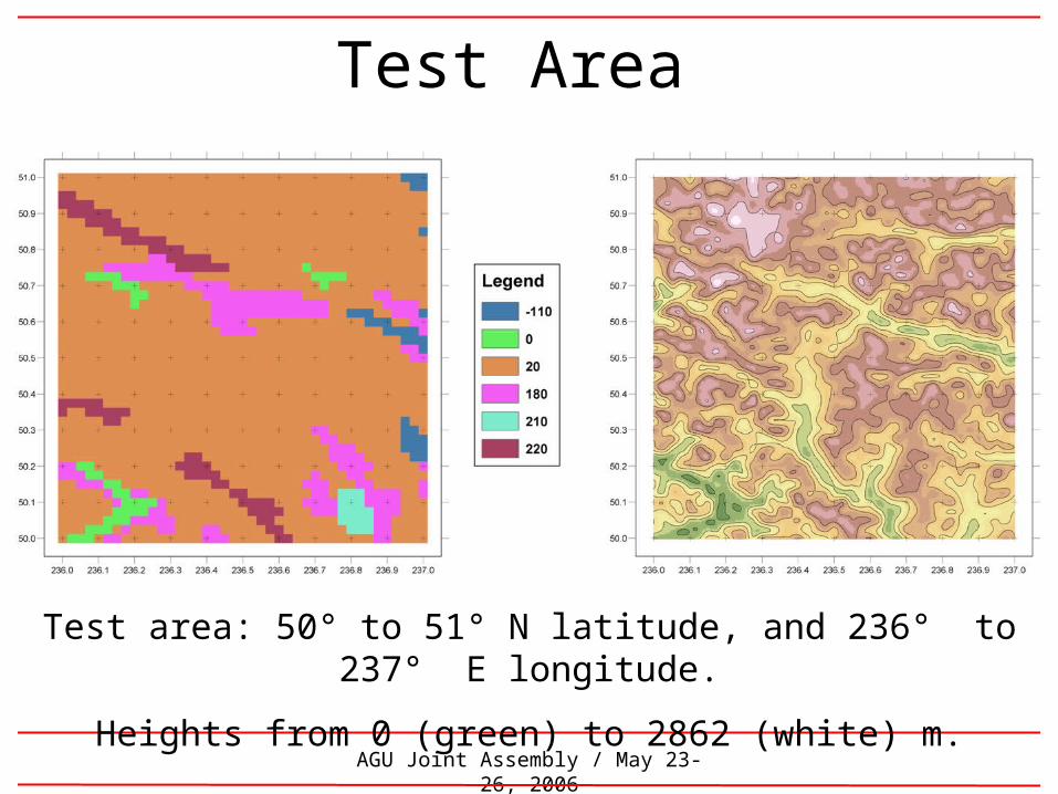
Test Area

Test area: 50° to 51° N latitude, and 236° to 237° E longitude.

Heights from 0 (green) to 2862 (white) m.

AGU Joint Assembly / May 23-26, 2006

Simulation B1

Values from 0 (red) to 5.7 (blue) cm, 1 cm contours.

Cone

AGU Joint Assembly / May 23-26, 2006

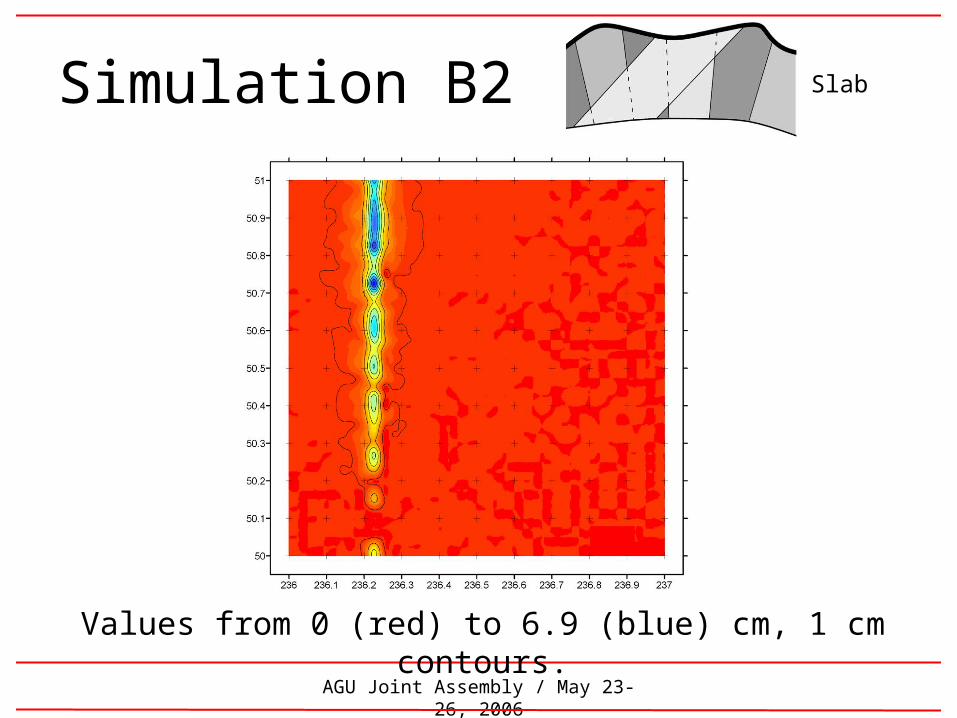
Simulation B2

Values from 0 (red) to 6.9 (blue) cm, 1 cm contours.

Slab

AGU Joint Assembly / May 23-26, 2006

Simulation B3

Values from 0 (red) to 7.9 (blue) cm, 1 cm contours.

Wedge

AGU Joint Assembly / May 23-26, 2006

Simulation A1

Values from -1.2 (green) to 1.2 (red) cm, 1 cm contours.

θ=45°

AGU Joint Assembly / May 23-26, 2006

Simulation A2

Values from -1.7 (green) to 1.6 (red) cm, 1 cm contours.

θ=30°

AGU Joint Assembly / May 23-26, 2006

Simulation A3

Values from -2.3 (green) to 2.6 (red) cm, 1 cm contours.

θ=15°

AGU Joint Assembly / May 23-26, 2006

Summary of Results

SimulationMax(cm)

Min(cm)

Height where cm level is reached

(m)

% of points with cm level corrections

(%)

B1: Cone 5.7 0 2403 11.2

B2: Slab 6.9 0 1051 13.0

B3: Wedge 7.9 0 1073 12.1

A1: θ=45° 1.2 -1.2 2250 12.6

A2: θ=30° 1.6 -1.7 1803 12.6

A3: θ=15° 2.6 -2.3 1543 13.5

AGU Joint Assembly / May 23-26, 2006

Conclusions

– Shortcomings are largest for regional phenomena.

– Shortcomings are only significant close to their source.

– More realistic estimates of shortcomings reach up to ~3 cm, but are only > 1 cm (in the test area) at elevations above ~1500 m.

– There do exist limited areas where these shortcomings may be significant, in terms of rigorous orthometric heights. Effects on e.g. geoid heights have yet to be evaluated.

AGU Joint Assembly / May 23-26, 2006

Acknowledgements

We would like to acknowledge NSERC and for their funding of this

research.