AIM-120C-5 Performance Brief - Zarettozaretto.com/sites/zaretto.com/files/missile-aerodynamic...1 AIM-120C-5 Performance Assessment for Digital Combat Simulation Enhancement Revision

1

AIM-120C-5 Performance Assessment

for Digital Combat Simulation Enhancement

Revision 2

September 2014

By

Thomas Tyrell, United Kingdom

Christian Funk, United States of America

Nagy Marton, Hungary

For questions regarding the assessment performed:

[email protected]

2

Table of Contents

List of Figures 3

1. Introduction 5

2. Physical Description of the AIM-120C-5 AMRAAM 5

3. Thrust of the missile 6

4. Aerodynamic Performance 9

4.1 Mesh Testing 10

4.2 Establishing Coefficient of Drag, Cd 13

4.1 Level Flight Performance 16

4.2 Missile under g load 21

4.3 Simulation Conclusion 30

5. Example Loft scenarios 31

5.1 Scenario 1 - Estimated real world scenario 31

5.2 Scenario 2 - Estimated maximum possible performance 33

5.3 Scenario 3 - Estimated low altitude performance 35

5.4 Scenario 4 - Experimentation with ascent/descent angles 37

7. Conclusions 39

8. Recommendations 40

9. Equations Used 41

10. References 43

11. Disclaimer 44

12. Appendix A - Distance and Time vs. Mach Number 45

3

List of Figures

Figure 1. - ATK motor cross-section 6

Figure 2. - CAD estimation of motor casing geometry 6

Figure 3. - Motor section total mass and CG 7

Figure 4. - CAD iteration of AMRAAM Motor body with fuel (yellow, 51.01 kg shown) 7

Figure 5. Cd-On/Cd Graph 9

Figure 6. Meshing of the flow field 10

Figure 7. Surface density is greatly refined for better accuracy 10

Figure 8. Orthogonality Test 1 11



Figure 11. CD as a function of v graph 13

Figure 12. CL as a function of v 14

Figure 13. CL as a function of AoA 15

Figure 14. Cd as a function of v 15

Figure 15. Straight Flight Performance M0.83 17




Figure 19. Separation Image 1 21



Figure 22. Constant g at 500m ASL 24



4




Figure 28. Loft Scenario 1 32




Figure 32 - AIM-120C Burn Test, 10km, 45kg fuel, 7sec burn 45

Figure 33 - AIM-120C Burn Test, 10km, 50kg fuel, 7sec burn 45

Figure 34 - AIM-120C Burn Test, 10km, 50kg fuel, 7.75sec burn 46

5

1. Introduction

This is the performance assessment of the Raytheon AIM-120C-5 AMRAAM. The goal of this report

is to evaluate the missile based on available technical data in order to improve the simulated

performance of the missile in Digital Combat Simulator. The information contained in this document

is from declassified sources, engineering analysis and computational fluid dynamics (CFD)

simulations. The missile's geometry and aerodynamic characteristics were modelled as accurately as

possible without having access to classified sources.

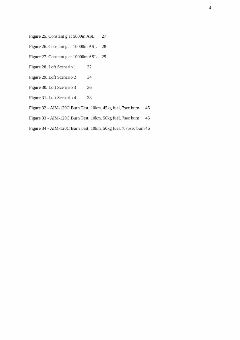
2. Physical Description of the AIM-120C-5 AMRAAM

Length 3650mm

Diameter 180mm

Forward Fin Span 482mm

Aft Fin Span 482mm

Total Mass 157kg

Table 1. Physical dimensions (nominal) of the missile [1][2]

There are discrepancies in the missile’s parameters in various sources. For example, source [1]

lists the

mass of the missile higher than source [2]

. Source two was chosen for the performance assessment case

study because of the reduced warhead mass, in addition to the smaller fins between these two sources.

6

Figure 1. - ATK motor cross-section

Figure 2. - CAD estimation of motor casing geometry

3. Thrust of the missile

The mass of missile’s rocket motor section is 75.34kg. It houses a single all-boost motor which uses a

reduced smoke hydroxyl-terminated poly-butadiene (HTPB) binder as its fuel.[3]

The type and ratio of chemicals used in the HTPB binder are unknown, but it is classified as a reduced

smoke propellant. Primarily solid propellant HTPB uses ammonium perchlorate (AP) as the oxidizer

and aluminum (Al) as the high energy fuel. According to Sutton [4]

, the Isp range for this type of fuel is

260-265, which is dependent upon the ratios of AP/Al. The higher the Al, the higher the Isp, but also

high smoke output [5]

. Due to the high performance requirement of the fuel, 265Isp was chosen.

Using the known density of the fuel (1.85g/cm^3)[4]

, it is possible to calculate the mass of the fuel if

the volume of the fuel chamber is known. To do this, ATK's design cross section (Figure 1) for their

rocket motor were used and an estimated creation was constructed in CAD (Figure 2).

7

Figure 3. - Motor section total mass and CG

Figure 4. - CAD iteration of AMRAAM Motor body with fuel (yellow, 51.01 kg shown)

8

The CAD model was designed to match the rocket motor's reported mass of 75.34kg[3]

, as Figure 3

illustrates.

From this the estimated fuel geometry was inserted, and using the known density a total fuel mass of

51.01kg was generated. The actual mass is dependent upon two key and unknown variables. Firstly

the exact density of the fuel (ratios of Al in the HTPB) and secondly what configuration the grain is

cast in.

The duration of the motor is the final assumption that must be made. All estimates of the AIM-120A

suggest it's boost stage duration is 6s, whilst it's sustain stage lasts 5s. Since the C-5 has more fuel

than the A[6]

, and as it is a boost only motor, this puts the estimated burn time between 7 and 9s.

Since it is a Mach 4+ capable missile, CFD simulations were run to help validate the fuel mass and

burn time. The simulations were run with several set parameters: Isp 265, mass between 50-52kg,

burn time between 6-9s. Figure 32, Figure 33 and Figure 34 in the appendix show the most likely

candidates with the set requirements; these match the CAD estimations as well as literary sources.

Ammendment: Source for the mass of the fuel has been found and now known to be 51.2559kg[7]

.

However, the below information is what was used for all the rest of the document.

To progress with the project, an assumption had to be made based off of all reasonable information.

Ultimately it was a fuel mass of 50kg, 265Isp and a 7.75s burn time providing the missile with a total

thrust of 16771.9N of thrust.

If the genuine fuel mass is closer to the CAD estimates then the only conclusion is that the Isp is

higher than public sources can demonstrate.

9

4. Aerodynamic Performance

The chosen method of determining the drag coefficients of the AMRAAM was CFD. The generic

CFD inaccuracy is said to be +/- 10%, which originates mostly from nonlinearities and simplifications

in the turbulence model of the flow. In a supersonic flow the largest nonlinearity is at the bow shock

of the object which is both a pressure, velocity and temperature jump, while the turbulence modelling

affects the onset of separations and the dissipation of vortices. The largest vortex system is located at

the end of the missile after the rocket motor finishes firing. While the motor is operational, the flow

around the back of the missile is different, which yields a reduction of the drag coefficient between 2-

20%. The variation in drag coefficient is dependent on velocity, altitude and angle of attack of the

AMRAAM in flight. Figure 5 shows the ratio of the drag coefficients in the engine-off and engine-on

configurations, and at various angles of attack.

Figure 5. Cd-On/Cd Graph

0.6

0.65

0.7

0.75

0.8

0.85

0.9

0.95

1

1.05

200 300 400 500 600 700 800 900 1000 1100 1200

CD

-On /

CD

[-]

v [m/s]

CD-On /CD as a function of velocity at various AoAs and h=5km

0 deg 30 deg 15 deg

10

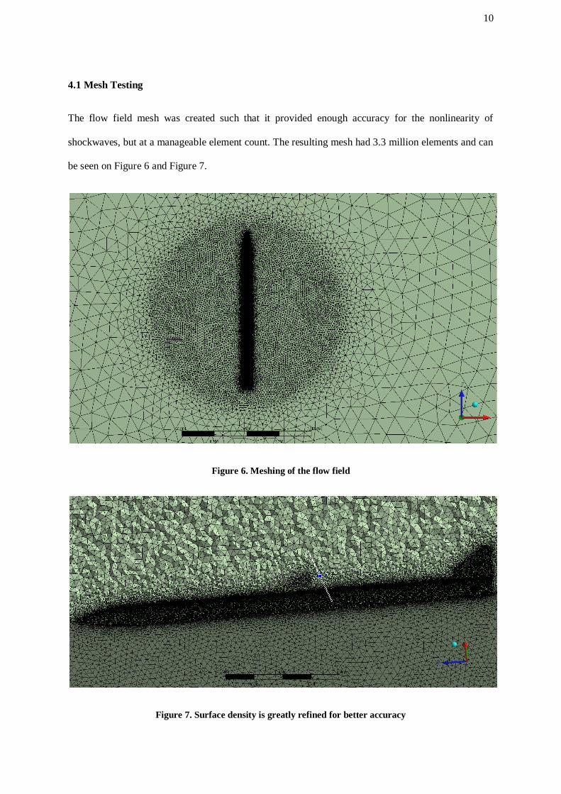
4.1 Mesh Testing

The flow field mesh was created such that it provided enough accuracy for the nonlinearity of

shockwaves, but at a manageable element count. The resulting mesh had 3.3 million elements and can

be seen on Figure 6 and Figure 7.

Figure 6. Meshing of the flow field

Figure 7. Surface density is greatly refined for better accuracy

11

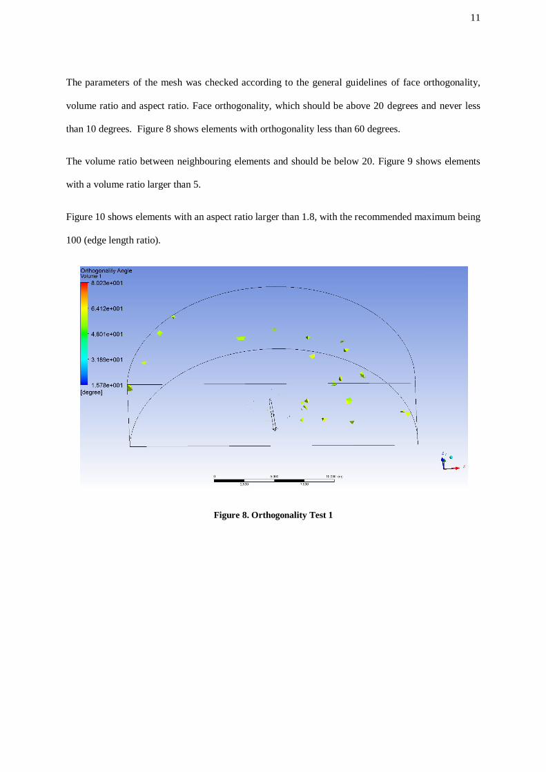
The parameters of the mesh was checked according to the general guidelines of face orthogonality,

volume ratio and aspect ratio. Face orthogonality, which should be above 20 degrees and never less

than 10 degrees. Figure 8 shows elements with orthogonality less than 60 degrees.

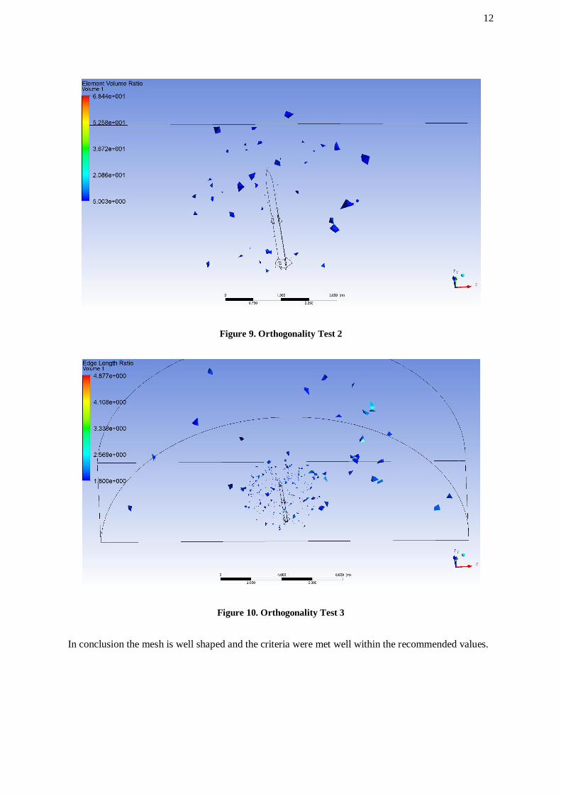
The volume ratio between neighbouring elements and should be below 20. Figure 9 shows elements

with a volume ratio larger than 5.

Figure 10 shows elements with an aspect ratio larger than 1.8, with the recommended maximum being

100 (edge length ratio).

Figure 8. Orthogonality Test 1

12



In conclusion the mesh is well shaped and the criteria were met well within the recommended values.

13

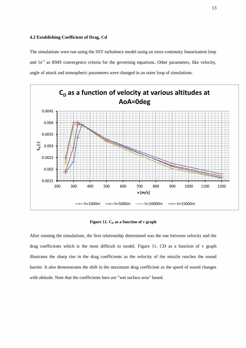
4.2 Establishing Coefficient of Drag, Cd

The simulations were run using the SST turbulence model using an extra continuity linearization loop

and 1e-5

as RMS convergence criteria for the governing equations. Other parameters, like velocity,

angle of attack and atmospheric parameters were changed in an outer loop of simulations.

Figure 11. CD as a function of v graph

After running the simulations, the first relationship determined was the one between velocity and the

drag coefficients which is the most difficult to model. Figure 11. CD as a function of v graph

illustrates the sharp rise in the drag coefficients as the velocity of the missile reaches the sound

barrier. It also demonstrates the shift in the maximum drag coefficient as the speed of sound changes

with altitude. Note that the coefficients here are "wet surface area" based.

0.0015

0.002

0.0025

0.003

0.0035

0.004

0.0045

200 300 400 500 600 700 800 900 1000 1100 1200

CD [

-]

v [m/s]

CD as a function of velocity at various altitudes at AoA=0deg

h=1000m h=5000m h=10000m h=15000m

14

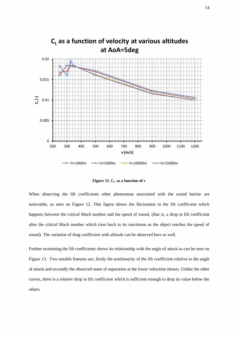
Figure 12. CL as a function of v

When observing the lift coefficients other phenomena associated with the sound barrier are

noticeable, as seen on Figure 12. This figure shows the fluctuation in the lift coefficient which

happens between the critical Mach number and the speed of sound, (that is, a drop in lift coefficient

after the critical Mach number which rises back to its maximum as the object reaches the speed of

sound). The variation of drag coefficient with altitude can be observed here as well.

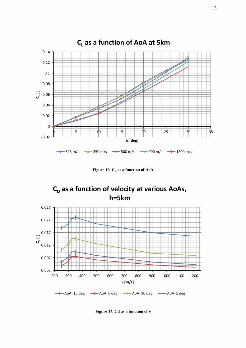
Further examining the lift coefficients shows its relationship with the angle of attack as can be seen on

Figure 13. Two notable features are, firstly the nonlinearity of the lift coefficient relative to the angle

of attack and secondly the observed onset of separation at the lower velocities shown. Unlike the other

curves, there is a relative drop in lift coefficient which is sufficient enough to drop its value below the

others.

0

0.005

0.01

0.015

0.02

200 300 400 500 600 700 800 900 1000 1100 1200

CL [

-]

v [m/s]

CL as a function of velocity at various altitudes at AoA=5deg

h=1000m h=5000m h=10000m h=15000m

15

Figure 13. CL as a function of AoA

Figure 14. Cd as a function of v

-0.02

0

0.02

0.04

0.06

0.08

0.1

0.12

0.14

0 5 10 15 20 25 30 35

CL [

-]

α [deg]

CL as a function of AoA at 5km

325 m/s 350 m/s 500 m/s 900 m/s 1200 m/s

0.002

0.007

0.012

0.017

0.022

0.027

200 300 400 500 600 700 800 900 1000 1100 1200

CD [

-]

v [m/s]

CD as a function of velocity at various AoAs, h=5km

AoA=15 deg AoA=0 deg AoA=10 deg AoA=5 deg

16

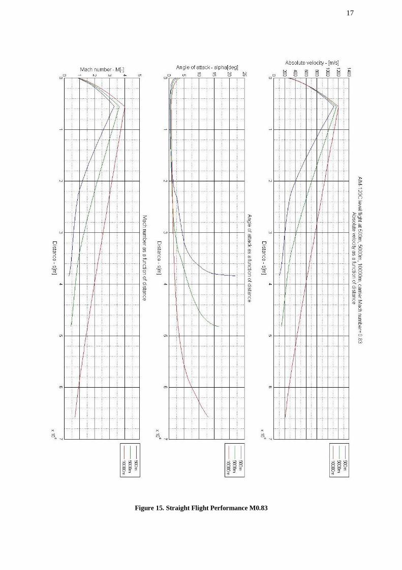
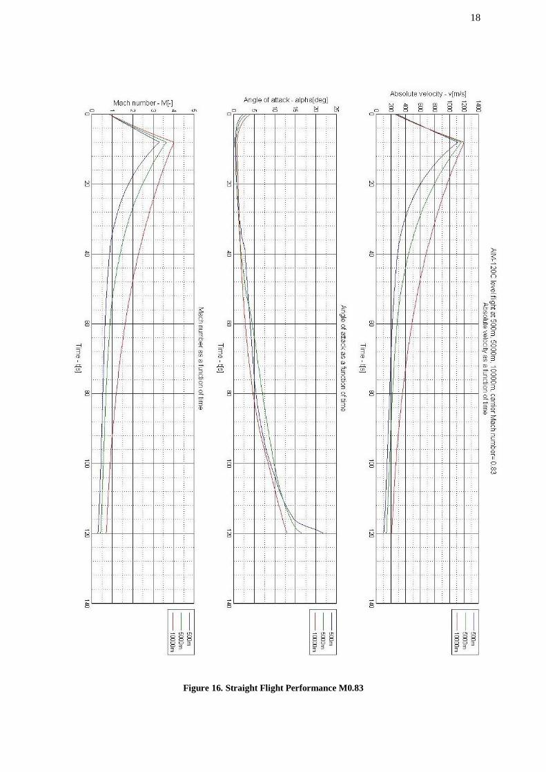
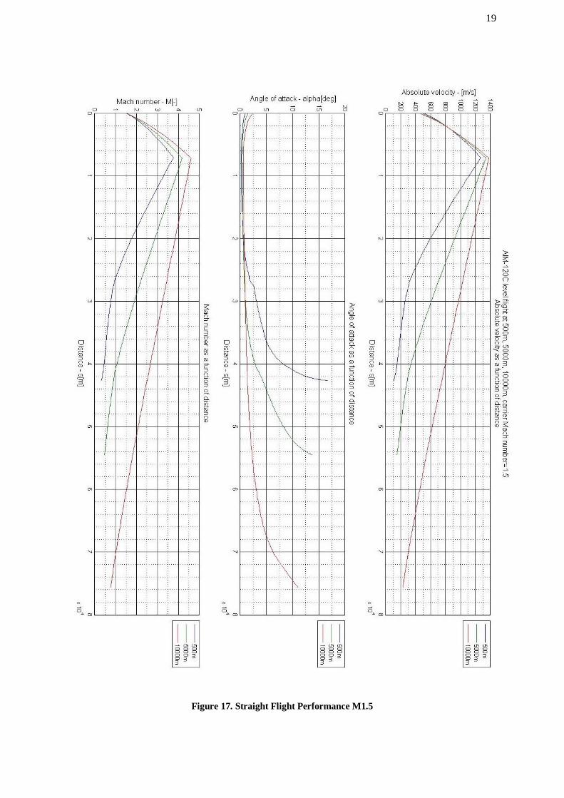
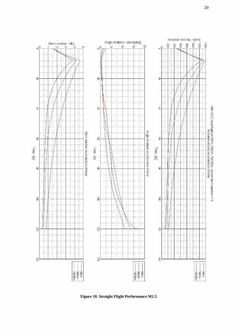
4.1 Level Flight Performance

Using the results from the simulations, the following graphs were produced for level flight of the

missile. This provides a benchmark of how quickly the missile accelerated and decelerated while

under normal g load at various altitudes.

Comparing Figure 16 and Figure 18, the difference between trans-sonic launches and supersonic

launches offers approximately 15% more range.

17

Figure 15. Straight Flight Performance M0.83

18


19


20


21

4.2 Missile under g load

Once the data on level flight performance was compiled, investigation onto performance under

induced g began. To do this, a series of simulations that varied the AoA of the missile was performed.

The maximum AoA of the missile was chosen to be 30 degrees, because at this point, in certain roll

positions and velocities the flow around the fins of the missile separates as seen on Figure 19.

Figure 19. Separation Image 1

This image shows the turbulent kinetic energy of the flow and shows the transition of the boundary

layer on the bottom left anhedral fins very well; flow disruption starts at the turbulent boundary layer.

Then, the separating flow progresses to a spot above the fin that corresponds to an inflection in the

surface normal velocity profile. This causes an instability in the flow that develops into a separation

that results in a stalled fin.

22

One might ask why the turbulent kinetic energy is lower on the other rear fin, even though its angle of

attack is higher than the other’s. The answer is that at this velocity (350 ms-1

) the flow around these

fins turn span-wise due to its different orientation (large dihedral on the image). On the next Figure 20

we can note the leading edge vortices of the dihedral fins which shows the flow direction.


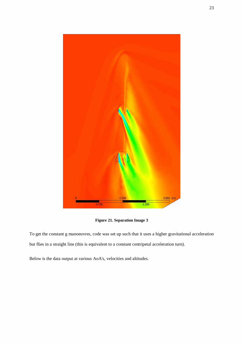
Contrast to this case is the next image Figure 21, that shows the missile at a higher velocity (500 ms-1

)

and shows how the anhedral fins have an attached flow and the dihedral ones are separated. It also

shows the “bow” shock of the missile and the shocks created by the fins.

23


To get the constant g manoeuvres, code was set up such that it uses a higher gravitational acceleration

but flies in a straight line (this is equivalent to a constant centripetal acceleration turn).

Below is the data output at various AoA's, velocities and altitudes.

24

Figure 22. Constant g at 500m ASL

25


26


27


28


29


30

4.3 Simulation Conclusion

The graphs show that the missile can hold 30g for 4.5s when starting at Mach 4. The reason behind

why the 30g curve stops at approximately 700ms-1 is because the AoA hit 30 degrees, and therefore

maintaining this g-load would be unobtainable.

The missile can maintain low g-loads whilst keeping its velocity at a comparable rate to level flight.

Even at trans-sonic velocities, the missile can still pull an upwards of 10g and hold it for 2.2 seconds.

This demonstrates that the missile can make intercepts at low velocities, illustrating its effective

range. From this it is possible to determine how far the missile is predicted to travel depending on the

specific launch parameters. Moreover is becomes evident how the missile loses its speed more quickly

as it begins to pull higher g-loads. It has been shown that higher altitude launches of AMRAAM lead

to much greater effective range, because the drag coefficients are lower. Next, the effects of missile

lofting is studied.

31

5. Example Loft scenarios

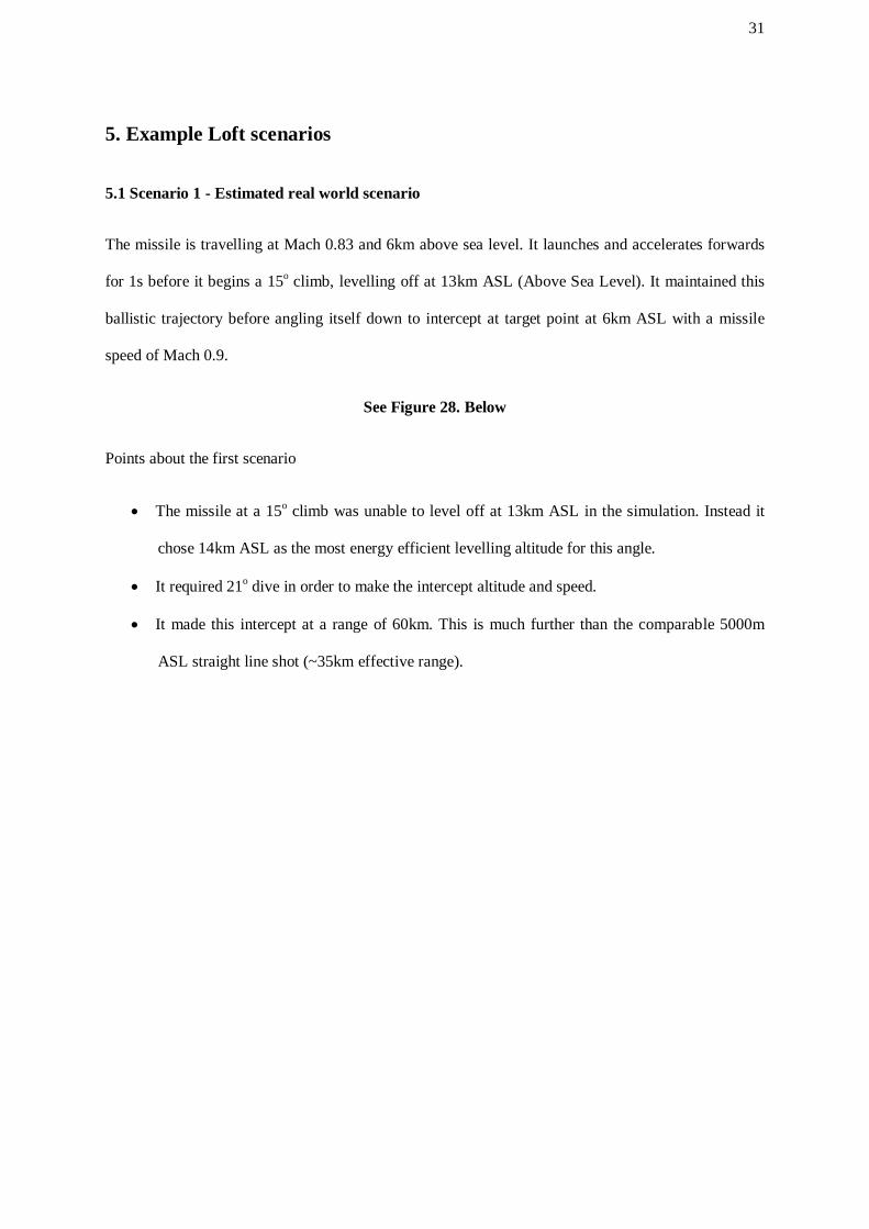
5.1 Scenario 1 - Estimated real world scenario

The missile is travelling at Mach 0.83 and 6km above sea level. It launches and accelerates forwards

for 1s before it begins a 15o climb, levelling off at 13km ASL (Above Sea Level). It maintained this

ballistic trajectory before angling itself down to intercept at target point at 6km ASL with a missile

speed of Mach 0.9.

See Figure 28. Below

Points about the first scenario

The missile at a 15o climb was unable to level off at 13km ASL in the simulation. Instead it

chose 14km ASL as the most energy efficient levelling altitude for this angle.

It required 21o dive in order to make the intercept altitude and speed.

It made this intercept at a range of 60km. This is much further than the comparable 5000m

ASL straight line shot (~35km effective range).

32

Figure 28. Loft Scenario 1

33

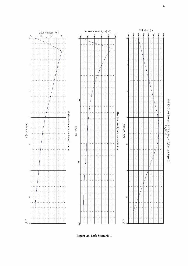
5.2 Scenario 2 - Estimated maximum possible performance

Using what was learnt above, the next test examined the maximum possible range of the missile in

realistic scenarios at missile parameter limits. The missile was launched at 13km at Mach 1.5 and

began its climb to 22km. It maintains this altitude before descending at angle that causes an

intersection at 6km at Mach 0.9

See Figure 29 below

Point about the second scenario

The ascent angle is still relatively low.

It demonstrates that the theoretical maximum realistic range of the missile on a stationary

point is approximately 90km.

34


35

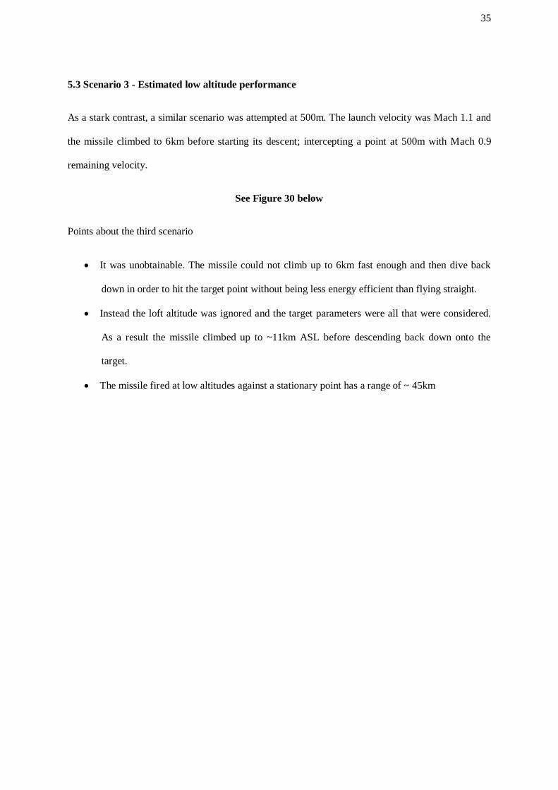
5.3 Scenario 3 - Estimated low altitude performance

As a stark contrast, a similar scenario was attempted at 500m. The launch velocity was Mach 1.1 and

the missile climbed to 6km before starting its descent; intercepting a point at 500m with Mach 0.9

remaining velocity.

See Figure 30 below

Points about the third scenario

It was unobtainable. The missile could not climb up to 6km fast enough and then dive back

down in order to hit the target point without being less energy efficient than flying straight.

Instead the loft altitude was ignored and the target parameters were all that were considered.

As a result the missile climbed up to ~11km ASL before descending back down onto the

target.

The missile fired at low altitudes against a stationary point has a range of ~ 45km

36


37

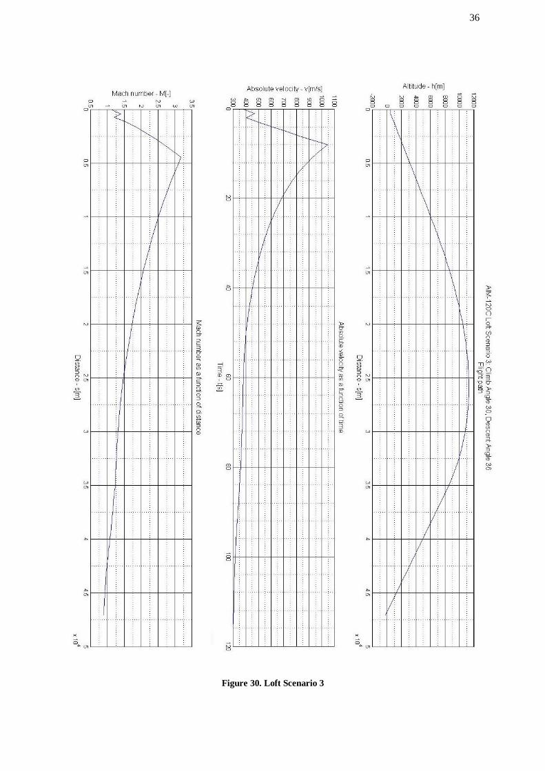
5.4 Scenario 4 - Experimentation with ascent/descent angles

Missile is launched at 6km ASL, Mach 0.83. It climbs at an angle of 30o and then descends at an angle

of 30o. This is to test to see how the missile behaves when only angles are considered.

See Figure 31 below

Points to consider

Without enforcing arbitrary loft altitudes, the missile will climb to a much greater height.

As a result the missile is able to maintain its velocity for longer due to much lower drag,

giving it a greater range.

In contrast to the rule enforced Loft Scenario 1. The missile reached approximately 90km with

the same target parameters. This is a 30km range boost.

38


39

7. Conclusions

After conducting the aerodynamic study of the capability of the AIM-120C-5 AMRAAM shape,

important physical phenomena were successfully reproduced according to the declassified references,

and no discrepancies were found in the results. Therefore, these simulations are as accurate as the

supporting mathematical and physical models are, and that also means the only way to get more

accurate than this is to measure it with physical experimentation.

A comparison of the calculated performance of the AMRAAM to the performance of in-game

employment of the AMRAAM shows that the missile is not properly modelled in Digital Combat

Simulator. Similarly, other missiles exhibit performance characteristics that are not representative of

their real performance. In some cases, this causes missiles to underperform; in other cases, missiles

such as the AMRAAM will over-perform their real flight characteristics.

In addition to the flight characteristics of the missile, the tracking capability of the missile was not

studied. The performance of radar and external or internal tracking hardware onboard the AMRAAM

was not studied in this assessment.

40

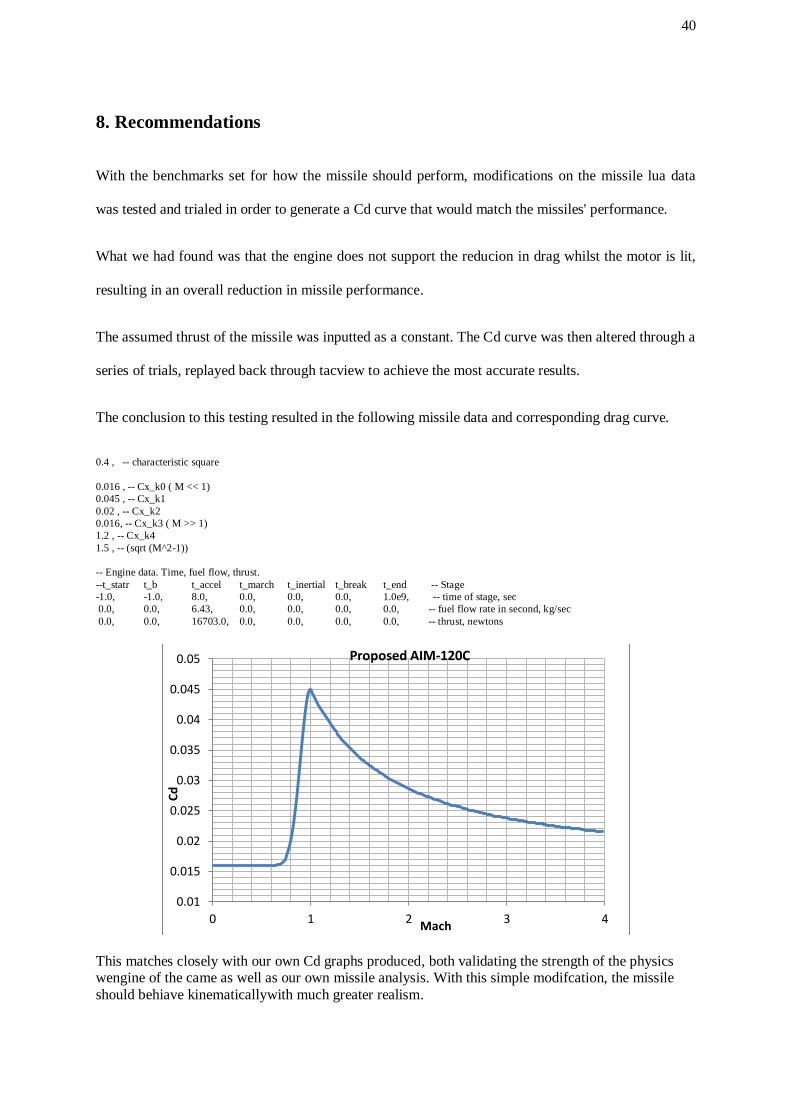
8. Recommendations

With the benchmarks set for how the missile should perform, modifications on the missile lua data

was tested and trialed in order to generate a Cd curve that would match the missiles' performance.

What we had found was that the engine does not support the reducion in drag whilst the motor is lit,

resulting in an overall reduction in missile performance.

The assumed thrust of the missile was inputted as a constant. The Cd curve was then altered through a

series of trials, replayed back through tacview to achieve the most accurate results.

The conclusion to this testing resulted in the following missile data and corresponding drag curve.

0.4 , -- characteristic square

0.016 , -- Cx_k0 ( M << 1)

0.045 , -- Cx_k1

0.02 , -- Cx_k2

0.016, -- Cx_k3 ( M >> 1)

1.2 , -- Cx_k4

1.5 , -- (sqrt (M^2-1))

-- Engine data. Time, fuel flow, thrust.

--t_statr t_b t_accel t_march t_inertial t_break t_end -- Stage

-1.0, -1.0, 8.0, 0.0, 0.0, 0.0, 1.0e9, -- time of stage, sec

0.0, 0.0, 6.43, 0.0, 0.0, 0.0, 0.0, -- fuel flow rate in second, kg/sec

0.0, 0.0, 16703.0, 0.0, 0.0, 0.0, 0.0, -- thrust, newtons

This matches closely with our own Cd graphs produced, both validating the strength of the physics wengine of the came as well as our own missile analysis. With this simple modifcation, the missile

should behiave kinematicallywith much greater realism.

0.01

0.015

0.02

0.025

0.03

0.035

0.04

0.045

0.05

0 1 2 3 4

Cd

Mach

Proposed AIM-120C

41

9. Equations Used

Eq 1. - Specific Impulse Equation

Eq. 2– Missile equation of motion

The flight path calculator uses a very simple 2D equation for the motion:

Where F is a vector of forces in the absolute coordinate system, m is the mass of the missile and g is

the gravitational acceleration.

Eq.3, Eq.4 Scalar components of the equation of motion.

In the 2D form we have two scalar equations:

and

Fx and Fy are projections of the lift, drag and thrust of the missile using simple trigonometric

functions.

Eq.5,Eq.6 Lift and drag force equation.

Lift and drag is calculated as usual:

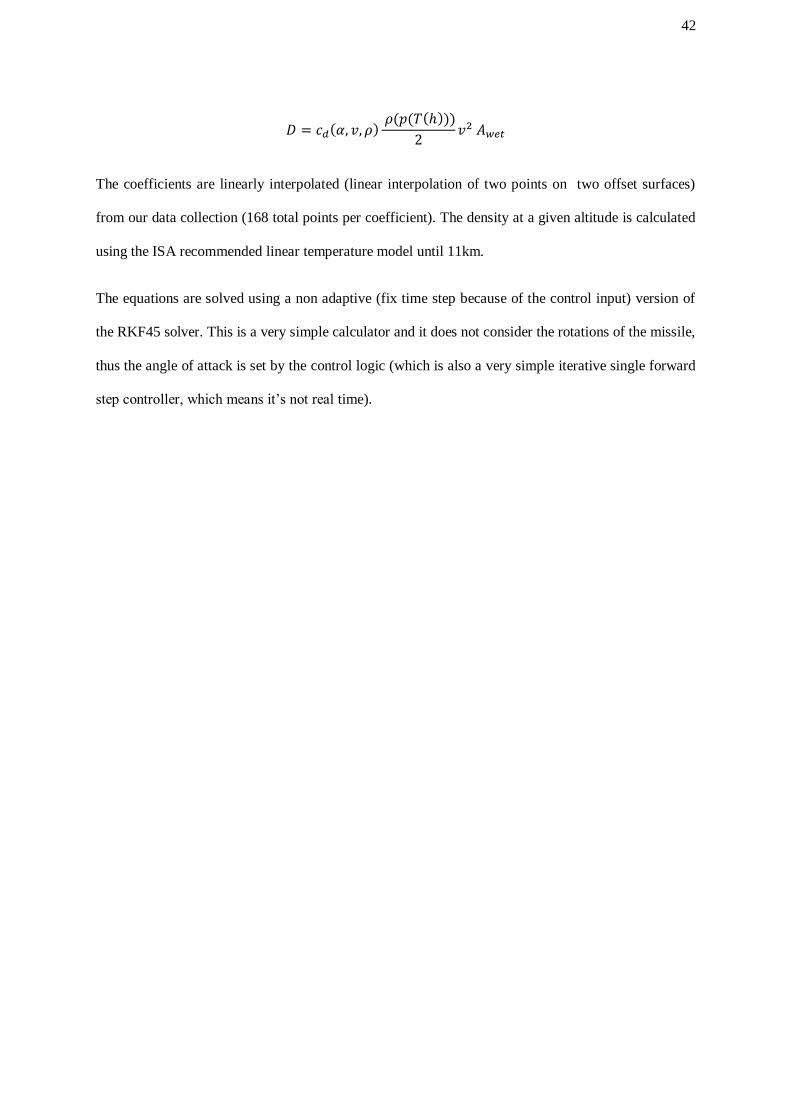
42

The coefficients are linearly interpolated (linear interpolation of two points on two offset surfaces)

from our data collection (168 total points per coefficient). The density at a given altitude is calculated

using the ISA recommended linear temperature model until 11km.

The equations are solved using a non adaptive (fix time step because of the control input) version of

the RKF45 solver. This is a very simple calculator and it does not consider the rotations of the missile,

thus the angle of attack is set by the control logic (which is also a very simple iterative single forward

step controller, which means it’s not real time).

43

10. References

[1] Air to Air Intercept Procedures Workbook Naval Air Training Command 2010

[2] Navy Training System Plan for the AIM-120 Advanced Medium Range Air-to-air Missile 1998

[3] AMRAAM PEP Propulsion System www.atk.com

[4] Rocket Propulsion Elements George, P, Sutton 2001

[5] Technologies for Future Precision Strike Missile Systems - Missile Aircraft Integration

[6] Distributed Simulation Testing for Weapons System Performance of the F/A-18 and AIM-120

AMRAAM 1998

[7] Hazard of Classification of Unite States Military Explosives ans Munitions Revision 14 2009

http://www.atk.com/

44

11. Disclaimer

We do not want to go to prison.

45

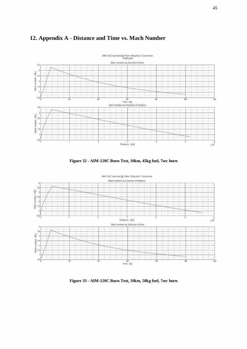
12. Appendix A - Distance and Time vs. Mach Number

Figure 32 - AIM-120C Burn Test, 10km, 45kg fuel, 7sec burn

Figure 33 - AIM-120C Burn Test, 10km, 50kg fuel, 7sec burn

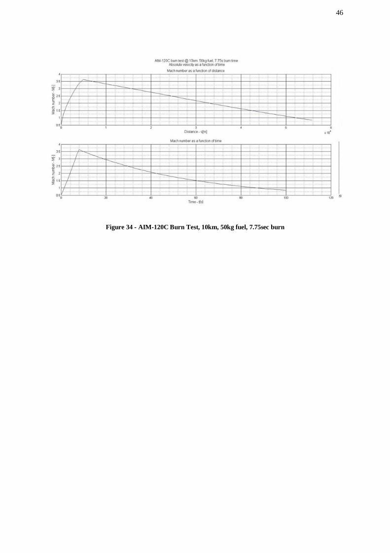
46

Figure 34 - AIM-120C Burn Test, 10km, 50kg fuel, 7.75sec burn

Documents

AIM-120C-5 Performance Brief - Zarettozaretto.com/sites/zaretto.com/files/missile-aerodynamic...1 AIM-120C-5 Performance Assessment for Digital Combat Simulation Enhancement Revision