Embed Size (px)
Citation preview

7/27/2019 AIM Manual
http://slidepdf.com/reader/full/aim-manual 1/66
Race Studio Analysis: user’s manual 1
Race Studio 2
Race Studio 2 Analysis
User’s manual
Version 1.00.10 – 9th June 2003

7/27/2019 AIM Manual
http://slidepdf.com/reader/full/aim-manual 2/66
Race Studio Analysis: user’s manual 2
AIM s.r.l. reserves the right to make changes in the content of this manual without obligation to notify
any person of such changes.
AIM s.r.l. shall not be liable for any errors contained herein or for incidental or consequential damages
in connection with the furnishing, performance or use of all the parts (hardware, software and
manuals).
Revision code: 1.00.10 – Dated 9th
June 2003.
Microsoft®, Windows® 98, Windows® 2000, Windows® XP, Windows® NT and Excel® are registered
trademark of Microsoft Corporation.
7/27/2019 AIM Manual
http://slidepdf.com/reader/full/aim-manual 3/66
Race Studio Analysis: user’s manual 3
Table of contents
TABLE OF CONTENTS...........................................................................................................................3
INTRODUCTION....................................................................................................................................5
What may I find in this manual? ....................................................................................................5
CHAPTER 1 - DATA ACQUISITION CONCEPTS......................................................................................6 1.1 – Analog and digital signals.....................................................................................................6
1.2 – Sampling rate ........................................................................................................................6
1.3 – Data analysis .........................................................................................................................6
1.4 – Frequency analysis ................................................................................................................7
CHAPTER 2 – SOFTWARE: GENERAL DESCRIPTION............................................................................8
2.1 – Getting started.......................................................................................................................8
2.1.1 – Before using data acquisition systems .............................................................................8
2.1.2 – Race Studio Analysis concepts ........................................................................................8
2.1.3 – Run the program...............................................................................................................9
2.2 Functionality ............................................................................................................................9 2.2.1 – Analysis window..............................................................................................................9
2.3 Data compatibility..................................................................................................................11
CHAPTER 3 – “HOW TO LOAD A TEST” .............................................................................................12
3.1 – Introduction: what is a database?.......................................................................................12
3.2 – How to load a test from the database..................................................................................12
3.2.1 – How to load a test using the selection criteria ...............................................................13
3.2.2 – How to load a test not using the selection criteria .........................................................14
3.3 – How to insert a test in the database ....................................................................................14
3.4 – How to modify the database test properties ........................................................................15
3.5 – How to delete a test from the database ...............................................................................15
3.6 – Which information are shown in the Lap manager layer....................................................16
3.7 – How to have more information about a test ........................................................................17
3.8 – How to close a test...............................................................................................................18
CHAPTER 4 – “HOW TO PLOT A TEST”..............................................................................................19
4.1 – How to plot a channel vs. time ............................................................................................19
4.2 – How to plot a channel vs. distance......................................................................................19
4.3 – How to plot a channel vs. frequency ...................................................................................20
4.4 – How to use the Measures and laps toolbar .........................................................................21
4.4.1 – How to add (remove) a channel to (from) a graph.........................................................22
4.4.2 – How to add (remove) the scale to (from) a graph..........................................................22
4.5 – How to change lap/plot more laps on the same graph........................................................22 4.5.1 – How to add (remove) a lap to (from) a graph and “multiple laps selection”.................22
4.5.2 – “How to” change lap/use the Laps toolbar ....................................................................23
4.6 – How to use the Measure information window.....................................................................24
4.6.1 – How to change the plotting scale ...................................................................................25
4.6.2 – How to shift/amplify a graph .........................................................................................25
4.6.3 – What can I do when sampled data are very noisy? ........................................................26
4.7 – How to change the graph colours .......................................................................................26
4.8 – How to change the plot settings ..........................................................................................27
4.8.1 – How to change the line width/cursor tags ......................................................................27
4.8.2 – How to use the “Shrink/Enlarge lap” checkbox.............................................................27
4.8.3 – How to change the background (grid/cursor) colour .....................................................28
4.9 – How to Zoom in/Zoom out a graph .....................................................................................28
4.10 – How to plot a X-Y graph ...................................................................................................28

7/27/2019 AIM Manual
http://slidepdf.com/reader/full/aim-manual 4/66
Race Studio Analysis: user’s manual 4
4.11 – How to change graph type.................................................................................................29
4.12 – Laps management..............................................................................................................29
4.12.1 – How to enable (disable) a lap.......................................................................................30
4.12.2 – How to insert a lap .......................................................................................................30
4.12.3 – How to merge a lap to the next one .............................................................................30
CHAPTER 5 – “HOW TO CREATE A TRACK MAP”..............................................................................31
5.1 – Introduction.........................................................................................................................31 5.2 – How to create a new map ....................................................................................................31
5.3 – Track map creation troubleshooting ...................................................................................33
5.4 – How to modify the reference speed .....................................................................................34
5.5 – How to import a map in the database .................................................................................34
5.6 – How to open a map from the database................................................................................35
5.7 – How to modify an existing map ...........................................................................................35
5.8 – How to shift the Start/Finish line ........................................................................................36
CHAPTER 6 – “HOW TO GET FURTHER INFORMATION FROM SAMPLED DATA” ..............................38
6.1 – Introduction.........................................................................................................................38
6.2 – How to plot a Histogram graph ..........................................................................................38 6.3 – How to use the Lap Times analysis .....................................................................................39
6.4 – How to use the Split Times analysis ....................................................................................39
6.5 – How to use the Channels report ..........................................................................................42
6.6 – How to use the Acceleration report.....................................................................................43
6.7 – How to use the Track report................................................................................................44
6.8 – How to use the Engine RPM analysis .................................................................................45
6.9 – How to use the Time compare analysis...............................................................................49
CHAPTER 7 – “HOW TO USE THE DATA ANIMATION FUNCTIONS” ...................................................51
7.1 – Introduction.........................................................................................................................51
7.2 – How to use the Data animation function.............................................................................51
7.3 – How to use the Lap replay command ..................................................................................51 7.4 – How to use the Dashboard function ....................................................................................52
CHAPTER 8 – “HOW TO USE THE MATH CHANNELS”.......................................................................55
8.1 – Introduction to Math channels ............................................................................................55
8.2 – Math channels window’s description..................................................................................55
8.2.1 – The predefined math channels .......................................................................................56
8.2.2 – The “Channel parameters” panel ...................................................................................57
8.2.3 – The “Formula” box ........................................................................................................57
8.2.4 – The “constants” table .....................................................................................................57
8.2.5 – The “Symbols & operators” table ..................................................................................58
8.2.6 – The “Identifiers” table....................................................................................................598.2.7 – The “Functions” table ....................................................................................................59
8.3 – How to add a predefined math channel...............................................................................61
8.4 – How to add a new math channel .........................................................................................62
CHAPTER 9 – UTILITY FUNCTIONS....................................................................................................63
9.1 – How to change the messages language...............................................................................63
9.2 – How to print a graph ...........................................................................................................63
9.3 – How to modify the unit of measures/wheel number ............................................................63
9.4 – How to save the windows status ..........................................................................................64
9.5 – How to load the windows status ..........................................................................................65
9.6 – How to export data in an Excel
®
compatible format...........................................................65 9.7 – How to load the user’s manual............................................................................................66
9.8 – How to run the AIM electronic documentation library.......................................................66

7/27/2019 AIM Manual
http://slidepdf.com/reader/full/aim-manual 5/66
Race Studio Analysis: user’s manual 5
Introduction
The Race Studio Analysis software is able to manage data coming from all the Aim data loggers. This
software has been designed and developed to analyze the data acquired by your gauge, in order to
improve the driver’s performances and the vehicle’s setup.
The aim of this manual is to allow everyone, even those who do not have a good knowledge of bothPersonal Computers and data analysis techniques, to correctly and usefully analyze the acquired data.
For this reason, this manual has been written using a “How to” technique, which consists in writing the
manual in order to answer the most frequently asked questions (concerning test loading, database
managing, plot settings, track map creating, etc…).
The manual has been written referencing to a Windows XP operative system.
What may I find in this manual?
Here in the manual you can find an exhaustive description of the Race Studio Analysis functions.Here below it is reported, more in details, the chapters’ description:
• Chapter 1 gives some general data acquisition concepts for an easier understanding of the data
acquisition systems.
• Chapter 2 gives a general description of the main functionalities of the Race Studio Analysis
software.
• Chapter 3 describes the “How to load a test” functions for the analysis of the recorded data
provided by Race Studio Analysis software.
• Chapter 4 describes the “How to plot a diagram” functions, explaining the different kinds of
diagrams available, the way to change line shape and colour, the zoom tool, etc.
• Chapter 5 concerns the “How to create/manage a map” utilities, showing how to create a newtrack map and how to load/delete/modify a previously created map.
• Chapter 6 describes a group of functions which allow the user to reach more detailed
information concerning a test session, like track report , setup analysis, histogram diagram,
maximum and minimum values for the measured channels, etc…
• Chapter 7 concerns the “Data animation” functions, which allow the user to have a graphical
replay of the acquired channels.
• Chapter 8 describes the “Math channels”: in particular, it will be explained how to create a new
math channel, how to load an existing one, how to define a new constant and how to test the
mathematic formula.
• Chapter 9 describes some utility functions, like “How to load/save the window status”, “Howto export a test in Microsoft Excel” and “How to modify the test preferences”.

7/27/2019 AIM Manual
http://slidepdf.com/reader/full/aim-manual 6/66
Race Studio Analysis: user’s manual 6
Chapter 1 - Data acquisition concepts
1.1 – Analog and digital signals
The measurement of a physical quantity, such as the speed of a car or the temperature of the exhaust
gas is at the same time a very simple and a very complex operation.
The first element necessary to the measurement is the sensor; it is a device that transforms a physical
quantity in an electrical signal.
An electrical signal may change between two fixed values or it may assume any value in a fixed range,
moreover it can be defined in a continuous time interval or in discrete time.
When a signal is defined in discrete time interval and can assume any value in a fixed range it is
named analog. When a signal is defined for finite time intervals and can assume only fixed values it is
named digital.
A data logger records and a Personal Computer elaborates only signals in a numerical (or digital) form,
for this reason it is necessary to convert all the signals in a digital form.
The data logger makes the conversion.
The sensors used for the measure of the number of engine revolutions and wheel speed provide anoutput signal assuming only fixed values and it is defined for a continuous time interval. The data
logger converts these signals in a digital form counting the impulses generated by the sensors.
All the other sensors, like potentiometers and thermocouples, have analog outputs. The data logger
again performs the analog-to-digital conversion.
1.2 – Sampling rate
The sampling rate is the data acquisition system’s recording frequency.
Although the output from the sensors changes continuously and instantaneously, the data acquisition
system records data at prefixed time intervals.The sampling rate is expressed in Hertz (Hz = 1/sec). For example if you have a sampling rate of 10
Hertz, it means that the input is read ten times per second and the time between any two successive
readings is 0.1 second.
For a correct representation of a physical phenomenon, like the travel of a suspension, it is very
important to read the output of the sensor a number of times enough to have no lost of information
about the phenomenon itself. So it is very important to select the right sampling rate.
1.3 – Data analysis
The analysis includes all the functions used to see and understand the recorded data.
The main analysis functions are plots, histograms and map generation.
The plots are the most common way to analyse data.
They show on the vertical axis the recorded values and on the horizontal axis the time or the distance
or the frequency.
The plots versus time and space are very easy to read because they show when and where data are
recorded. On the contrary plots versus frequency need some more explanations, which are given in
next paragraph.
All the analysis functions provided by the Race Studio Analysis software are described in Chapters
from 3 to 9.
7/27/2019 AIM Manual
http://slidepdf.com/reader/full/aim-manual 7/66
Race Studio Analysis: user’s manual 7
1.4 – Frequency analysis
The frequency analysis is based on the Fourier theorem. This theorem affirms that every signal can be
obtained as the sum of a number of finite or infinite sinusoids.
Three parameters give a full characterization of a sinusoid; they are 1) the frequency, 2) the amplitude
and 3) the phase.
Therefore each signal can be shown versus time as a sinusoids sum having different values of frequency, amplitude and phase.
The normal way to represent sinusoids against frequency is to show two different plots one for the
amplitude and another for the phase. They are named respectively amplitude spectrum and phase
spectrum.
The signals usually analysed with the Race Studio Analysis program have a very high number of
sinusoids’ components; the frequencies of these components are very close each other.
A much diffused application of the frequency analysis is to calculate the power spectrum of the signal.
The power spectrum is obtained squaring the amplitude of the different components of the signal.
In order to obtain the power spectrum in the frequency domain it is necessary to make the Fourier
Transform of the signal.
The Fourier Transform requires a lot of math operations. For this reason it is usually calculated with afast algorithm named Fast Fourier Transform (FFT). This algorithm reduces both the complexity and
the number of operations and thus the calculation time.
The Race Studio Analysis program allows calculating, using the Fast Fourier Transform, the power
spectrum for all the channels, both input and math. The power spectrum can be shown selecting the
“View-Plot vs. frequency” item from the View menu.
The power spectrum is very useful because it allows analysing the characteristic frequencies of the
signal. For the typical applications of the EVO 3 system, it is very interesting for the suspensions
analysis.

7/27/2019 AIM Manual
http://slidepdf.com/reader/full/aim-manual 8/66
Race Studio Analysis: user’s manual 8
Chapter 2 – Software: general description
2.1 – Getting started
2.1.1 – Before using data acquisition systems
The time invested before using data acquisition systems for the first time produces more accurate data
and a more reliable system.
Install the data logger, the sensors and the cables on the vehicle and the software on your Personal
Computer well in advance of the departure to the track; in case problems arise they can be solved.
Learn the Race Studio Analysis software using the manual and with some example tests.
Make a few trial runs of recording and downloading data in the shop.
2.1.2 – Race Studio Analysis concepts
Tests
The Race Studio Analysis software stores data downloaded from the data logger in files, they aredefined by the program tests. The user at the end of the download operation gives the name of the
tests. Changing the name of the tests outside the Race Studio 2 software may cause the tests to be no
more recognised by the program.
Database
The tests are recorded into directories created and named by the user; otherwise, if the user saves the
test without specifying the directory, the test file will be automatically saved in the “\Program
files\AIM\DATA”.
The downloaded tests are saved in a database. This database is characterized by 5 attributes, which
define the Vehicle, the Track, the Driver, the Championship and the Test type. For further information
concerning the tests database, please refer to chapter 3.
Channels
The Race Studio Analysis software allows analysing two different kinds of measures: Input channels
and Math channels.
The data logger acquires the Input channels (for example speed or oil pressure), while the user defines
the Math channels and the program calculates them on the Personal Computer using the Input
channels or the Math channels themselves (examples of math channels are linear acceleration or gear
number).
Reference speed
For tests on track the most important measure for the data acquisition systems is the speed. The speed
is necessary for starting to record data and for a lot of analysis functions like the creation of the map,
the plot vs. distance, the calculation of splits, the data animation and so on.
The Race Studio Analysis software has a special channel named Reference speed used as the official
speed channel of the test. Three input channels are provided to become the Reference speed , they are
speed #1, speed #2, and the analogue channel with the Pitot tube connected.
It is possible to select the Reference speed channel from the toolbar main menu inside the “Modify –
Reference speed” command. After the selection the selected channel becomes the official reference
speed channel for the current test and for the next downloaded ones. For further information
concerning the Reference speed , please refer to chapter 5.4.
7/27/2019 AIM Manual
http://slidepdf.com/reader/full/aim-manual 9/66
Race Studio Analysis: user’s manual 9
WARNING. If the Reference speed is not selected or the values of the Reference speed channel are
always zero during the analysis there is not visualisation referred to distance, for example Plot vs.
distance or Split report .
Maps
Maps are the tracks’ drawings. The calculation of the maps is performed using the Reference speed and lateral acceleration channels for four wheels vehicles or the Reference speed and the gyroscope for
two wheels vehicles (motorbikes). For a description of how to calculate a new map see chapter 5.
2.1.3 – Run the program
Run the program with a double click of the left button of the mouse over the shortcut to the Race
Studio Analysis software on the desktop of your computer, the shortcut has been created by the setup
program.
Otherwise run it from the Programs menu into the Start menu.
2.2 Functionality
The Race Studio Analysis software includes all the functions for the analysis of the downloaded data.
This chapter gives a short description of the main functions provided by the software for the analysis
of the recorded data.
Before to start describing the program functionality it is necessary to outline the principal window
shown running the Race Studio Analysis software from your PC’s desktop shortcut or from the Start
menu.
2.2.1 – Analysis window
Selecting the “Analysis” command, a dialog window for the selection of the test to analyse is
displayed. When the test is chosen the Analysis window is displayed; Fig. 2.1 shows it.
All loaded data are shown inside a window named Test database and Lap manager . If you close the
Test database and Lap manager window during the Analysis, the current test will be unloaded. It is
reminded that closing the Test database and Lap Manager window does not entail the closure of Race
Studio Analysis.
7/27/2019 AIM Manual
http://slidepdf.com/reader/full/aim-manual 10/66
Race Studio Analysis: user’s manual 10
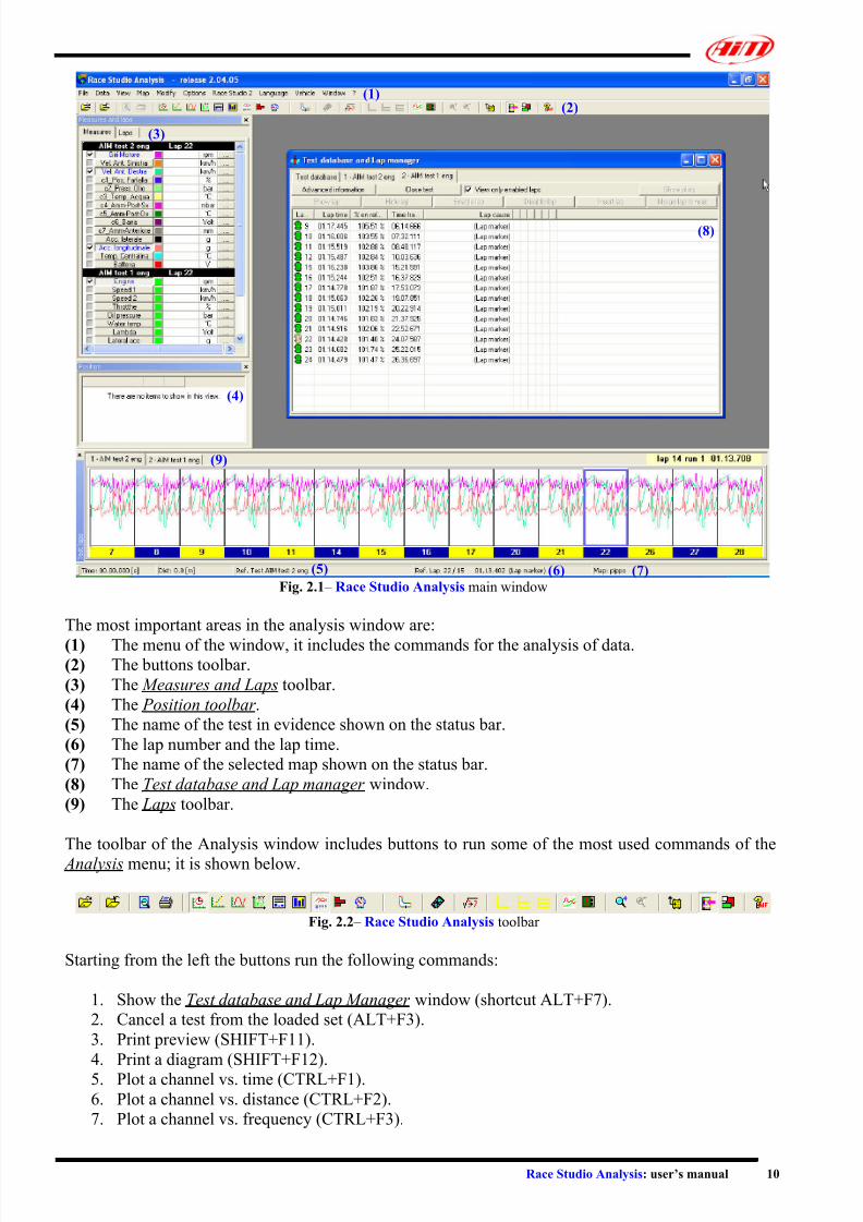
Fig. 2.1 – Race Studio Analysis main window
(1)(2)
(3)
(8)
(4)
(9)
(5) (6) (7)
The most important areas in the analysis window are:
(1) The menu of the window, it includes the commands for the analysis of data.(2) The buttons toolbar.
(3) The Measures and Laps toolbar.
(4) The Position toolbar .
(5) The name of the test in evidence shown on the status bar.
(6) The lap number and the lap time.
(7) The name of the selected map shown on the status bar.
(8) The Test database and Lap manager window.
(9) The Laps toolbar.
The toolbar of the Analysis window includes buttons to run some of the most used commands of the
Analysis menu; it is shown below.
Fig. 2.2 – Race Studio Analysis toolbar
Starting from the left the buttons run the following commands:
1. Show the Test database and Lap Manager window (shortcut ALT+F7).
2. Cancel a test from the loaded set (ALT+F3).
3. Print preview (SHIFT+F11).
4. Print a diagram (SHIFT+F12).
5. Plot a channel vs. time (CTRL+F1).
6. Plot a channel vs. distance (CTRL+F2).
7. Plot a channel vs. frequency (CTRL+F3).

7/27/2019 AIM Manual
http://slidepdf.com/reader/full/aim-manual 11/66
Race Studio Analysis: user’s manual 11
8. Plot a channel vs. channel (CTRL+F5).
9. Run the Split times analysis (CTRL+F6).
10. Run the Lap times report (CTRL+F7).
11. Run the Channels report.
12. Display a histogram of the selected channels (CTRL+F8).
13. Show the dashboard simulation (CTRL+F11).
14. Show the track map (SHIFT+F1).
15. Run the Data animation function (F12).
16. Math channels (ALT+F8).
17. Change plot style: overlapped graphs;
18. Change plot style: mixed graphs;
19. Change plot style: tiled graphs;
20. Plot settings dialog window (ALT+F9).
21. Measures info dialog window (ALT+F10).
22. Enable zoom (SHIFT+F9).
23. Disable zoom (SHIFT+F10).
24. Run Race Studio 2 (F5).
25. Toggle visibility of the Measures toolbar (ALT+F11).26. Load window status.
27. Online manual (F1).
All these commands will be described in chapters from 3 to 9.
2.3 Data compatibility
If it is necessary to analyse tests recorded with the WDrack software, it is possible when they have
been recorded with software version starting from the 3.00. These files will be opened and converted
to a format compatible with Race Studio Analysis; after this conversion, the files will no more becompatible with Wdrack .
If the tests include math channels they are lost during the conversion. It is possible to calculate them
again running the new user interface for the definition and calculation of math channels.
Race Studio Analysis is also able to open the tests downloaded with Race Studio 1; these files, unlike
the ones downloaded with the Wdrack software, will not be converted into another format.

7/27/2019 AIM Manual
http://slidepdf.com/reader/full/aim-manual 12/66
Race Studio Analysis: user’s manual 12
Chapter 3 – “How to load a test”
3.1 – Introduction: what is a database?
Race Studio 2 has a new and innovative tests storing system based on databases.
This storing system consists in saving the file specifying 5 characteristics (even called “attributes”).
Such information, which are saved together with the test file, are listed here below:
• Vehicle name
• Driver name
• Track name
• Championship
• Test type
When you insert a test in the database, the 5 characteristics you specified will be saved as “sub-
categories” (or attributes) of the 5 main database categories. In the following example, for instance, it
is reported two main categories (the driver name and the track name), each one composed of twosub-categories/attributes (Driver 1 and Driver 2 for the Driver name, Indianapolis and Monza for the
Track name):
• Driver
o Driver 1
o Driver 2
• Track
o Indianapolis
o Monza
This new test storing system is very useful as it allows the user both to divide the test files into self-
defined groups, each one characterized by 5 attributes, and to load the test files in a very practical and
easy way.
For further information concerning the database management, please refer to chapter 3.2.
3.2 – How to load a test from the database
Once run Race Studio Analysis, it will appear the Test database and Lap Manager window, as shown
in Figure 3.1. This window is divided into two separate rows:
• In the upper row there are 5 boxes, labelled from (7) to (11), showing the database’s “selection
criteria”. Each one of the 5 boxes has its own pushbutton (Select track (2), Select vehicle (3),
Select driver (4), Select championship (5) and Select test type (6), which is used to activate the
corresponding selection criterion. Checkbox (1) is used to enable/disable the selection criteria.
Button (18) is used to show the graphs when hidden by other windows.
• In the lower part of the Test database and Lap manager window it is reported the “available
tests” list (12), i.e. a list of all the tests included in the database. In particular, it is shown the
test name, the file data, the number of laps, the best lap time and the corresponding lap number,
the related database sub-categories and the file path. Moreover, in the lower part of the Test
database and Lap manager window, there are 5 buttons used to “Open a test” (13), to “Modify
the test properties” (14), to “Import a test in the database” (15), to “Remove a test from thedatabase” (16) and to “Export a test file” (17) (on a floppy disk, for instance).
7/27/2019 AIM Manual
http://slidepdf.com/reader/full/aim-manual 13/66
Race Studio Analysis: user’s manual 13
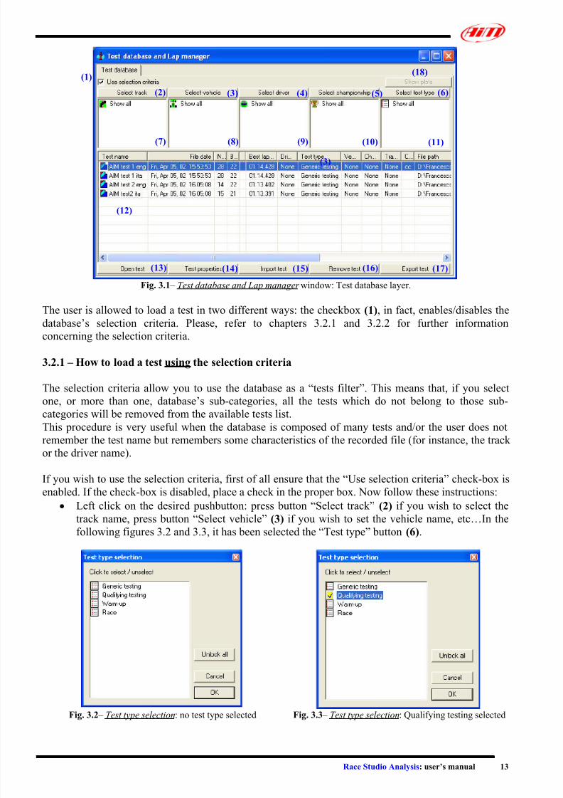
Fig. 3.1 – Test database and Lap manager window: Test database layer.
(18)(1)
(2) (6)(3) (4) (5)
(7) (8) (9) (10) (11)
(3)
(12)
(13) (16)(14) (15) (17)
The user is allowed to load a test in two different ways: the checkbox (1), in fact, enables/disables the
database’s selection criteria. Please, refer to chapters 3.2.1 and 3.2.2 for further information
concerning the selection criteria.
3.2.1 – How to load a test using the selection criteria
The selection criteria allow you to use the database as a “tests filter”. This means that, if you select
one, or more than one, database’s sub-categories, all the tests which do not belong to those sub-
categories will be removed from the available tests list.This procedure is very useful when the database is composed of many tests and/or the user does not
remember the test name but remembers some characteristics of the recorded file (for instance, the track
or the driver name).
If you wish to use the selection criteria, first of all ensure that the “Use selection criteria” check-box is
enabled. If the check-box is disabled, place a check in the proper box. Now follow these instructions:
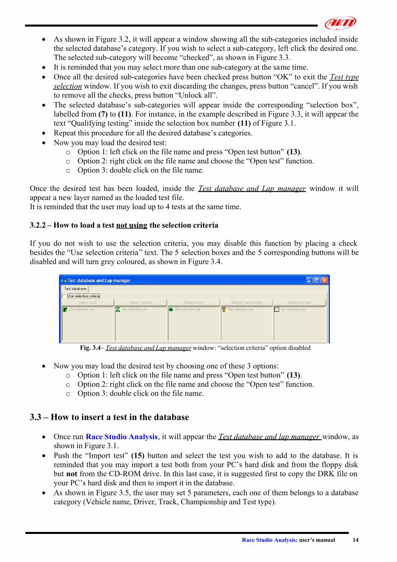
• Left click on the desired pushbutton: press button “Select track” (2) if you wish to select the
track name, press button “Select vehicle” (3) if you wish to set the vehicle name, etc…In the
following figures 3.2 and 3.3, it has been selected the “Test type” button (6).
Fig. 3.2 – Test type selection: no test type selected Fig. 3.3 – Test type selection: Qualifying testing selected
7/27/2019 AIM Manual
http://slidepdf.com/reader/full/aim-manual 14/66
Race Studio Analysis: user’s manual 14
• As shown in Figure 3.2, it will appear a window showing all the sub-categories included inside
the selected database’s category. If you wish to select a sub-category, left click the desired one.
The selected sub-category will become “checked”, as shown in Figure 3.3.
• It is reminded that you may select more than one sub-category at the same time.
• Once all the desired sub-categories have been checked press button “OK” to exit the Test type
selection window. If you wish to exit discarding the changes, press button “cancel”. If you wish
to remove all the checks, press button “Unlock all”.• The selected database’s sub-categories will appear inside the corresponding “selection box”,
labelled from (7) to (11). For instance, in the example described in Figure 3.3, it will appear the
text “Qualifying testing” inside the selection box number (11) of Figure 3.1.
• Repeat this procedure for all the desired database’s categories.
• Now you may load the desired test:
o Option 1: left click on the file name and press “Open test button” (13).
o Option 2: right click on the file name and choose the “Open test” function.
o Option 3: double click on the file name.
Once the desired test has been loaded, inside the Test database and Lap manager window it will
appear a new layer named as the loaded test file.It is reminded that the user may load up to 4 tests at the same time.
3.2.2 – How to load a test not using the selection criteria
If you do not wish to use the selection criteria, you may disable this function by placing a check
besides the “Use selection criteria” text. The 5 selection boxes and the 5 corresponding buttons will be
disabled and will turn grey coloured, as shown in Figure 3.4.
Fig. 3.4 – Test database and Lap manager window: “selection criteria” option disabled
• Now you may load the desired test by choosing one of these 3 options:
o Option 1: left click on the file name and press “Open test button” (13).
o Option 2: right click on the file name and choose the “Open test” function.
o Option 3: double click on the file name.
3.3 – How to insert a test in the database
• Once run Race Studio Analysis, it will appear the Test database and lap manager window, as
shown in Figure 3.1.
• Push the “Import test” (15) button and select the test you wish to add to the database. It is
reminded that you may import a test both from your PC’s hard disk and from the floppy disk
but not from the CD-ROM drive. In this last case, it is suggested first to copy the DRK file on
your PC’s hard disk and then to import it in the database.
• As shown in Figure 3.5, the user may set 5 parameters, each one of them belongs to a databasecategory (Vehicle name, Driver, Track, Championship and Test type).

7/27/2019 AIM Manual
http://slidepdf.com/reader/full/aim-manual 15/66
Race Studio Analysis: user’s manual 15
Fig. 3.5 – Add test to database window Fig. 3.6 – Add/Modify test attributes window
If the database is blank or you wish to set a new database sub-category (i.e. attribute), please follow
these instructions:
• To set the Vehicle name, please push the Add/Modify button which corresponds to the Vehicle
row. It will appear the window shown in Figure 3.6.
• Now, please fill the upper right corner box with the correct vehicle name and, then, click the
“<< Add value to database” pushbutton. The vehicle name will appear in the vehicle namecolumn.
• Once added the value to the database, the OK pushbutton will become enabled: please, select
the desired vehicle name from the vehicle name column and, then, click button OK.
• Please, repeat this procedure for the other 4 database categories (i.e. Driver name, Track,
Championship and Test type).
Otherwise, if the database is not blank and the user wishes to add the test in a previously set database
sub-category, please follow these instructions:
• From the Add test to database window, instead of pressing the “Add/Modify” button, select the
desired vehicle name from the corresponding “combo” menu, located in the middle of Figure3.5.
• Repeat this procedure for the other 4 database categories.
3.4 – How to modify the database test properties
In order to modify the test properties, please select the desired test (single-click on the test name), and
then press button Test properties. It will appear the Test information setting window, as shown in
Figure 3.5.
The procedure to be followed is similar to the one described in chapter 3.3 “How to insert a test in the
database”: the test may be either moved in a new database sub-categories or in a previously createdone.
3.5 – How to delete a test from the database
If you wish to delete a test from the database, please enter the Test database and Lap manager , shown
in Figure 3.1, and select the test you wish to delete by single-clicking on the test name.
Once the test has been selected, you may either push button “Remove test” or right click on the file
name and choose “Delete test from database” function.
The test will be automatically removed from the database but will not be deleted from your PC’s
hard disk , as reminded in the confirmation window, shown in Figure 3.6, which appears on your PC’s
monitor.
7/27/2019 AIM Manual
http://slidepdf.com/reader/full/aim-manual 16/66
Race Studio Analysis: user’s manual 16
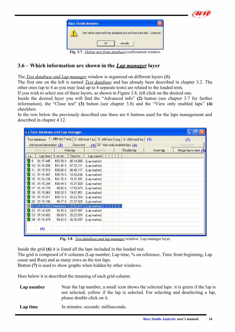
Fig. 3.7 – Delete test from database confirmation window.
3.6 – Which information are shown in the Lap manager layer
The Test database and Lap manager window is organized on different layers (1).
The first one on the left is named Test database and has already been described in chapter 3.2. The
other ones (up to 4 as you may load up to 4 separate tests) are related to the loaded tests.
If you wish to select one of these layers, as shown in Figure 3.8, left click on the desired one.
Inside the desired layer you will find the “Advanced info” (2) button (see chapter 3.7 for further
information), the “Close test” (3) button (see chapter 3.8) and the “View only enabled laps” (4)
checkbox.
In the row below the previously described one there are 6 buttons used for the laps management anddescribed in chapter 4.12.
Fig. 3.8 – Test database and lap manager window: Lap manager layer.
(1) (7)
(2) (4)(3)
(5)
(6)
Inside the grid (6) it is listed all the laps included in the loaded test.
The grid is composed of 6 columns (Lap number, Lap time, % on reference, Time from beginning, Lap
cause and Run) and as many rows as the test laps.
Button (7) is used to show graphs when hidden by other windows.
Here below it is described the meaning of each grid column:
Lap number Near the lap number, a small icon shows the selected laps: it is green if the lap is
not selected, yellow if the lap is selected. For selecting and deselecting a lap, please double click on it.
Lap time In minutes: seconds: milliseconds.
7/27/2019 AIM Manual
http://slidepdf.com/reader/full/aim-manual 17/66
Race Studio Analysis: user’s manual 17
% on reference The best lap (the one with the lowest lap time) is considered the Reference Lap.
It is possible to change the reference lap, deselecting it and selecting another lap.
Time from the
beginning
Time from the beginning of the test. In minutes: seconds: milliseconds.
Lap cause A lap may be: Lap marker, First lap, Vehicle stop, Computed merging two
laps, Computed splitting a lap or Calculated lap. This last possibility, veryrare, means that there is an incompatibility between the value of the lap and the
number of samples recorded: the lap time is so recalculated, considering some
check points that the logger puts inside the data.
The Computed splitting a lap/merging two laps lap causes are shown when the
Merge to next lap/Insert lap options are used.
The old files, where the lap cause was not specified, show simply Generic lap.
Run In a test you may have one or more Runs. Whenever the car stops for more than
a few seconds, the Run counter is incremented. In this way it is possible to divide
the data in accordance with the different test runs.
Split # These cells show the split times sampled by your data logger. AIM gauges, such
as MyChron 3 Basic/Plus/Gold, are able to record up to 5 split times.
As shown in Figure 3.8, the laps are listed from the 1 st to the last one.
• If you click on the “Lap number” box, the laps will be displayed from the last to the 1 st one.
• If you click on the “Lap time” box, the laps will be listed from the fastest to the lowest. If you
click again on the “Lap time” box, the laps will be shown in the opposite order.
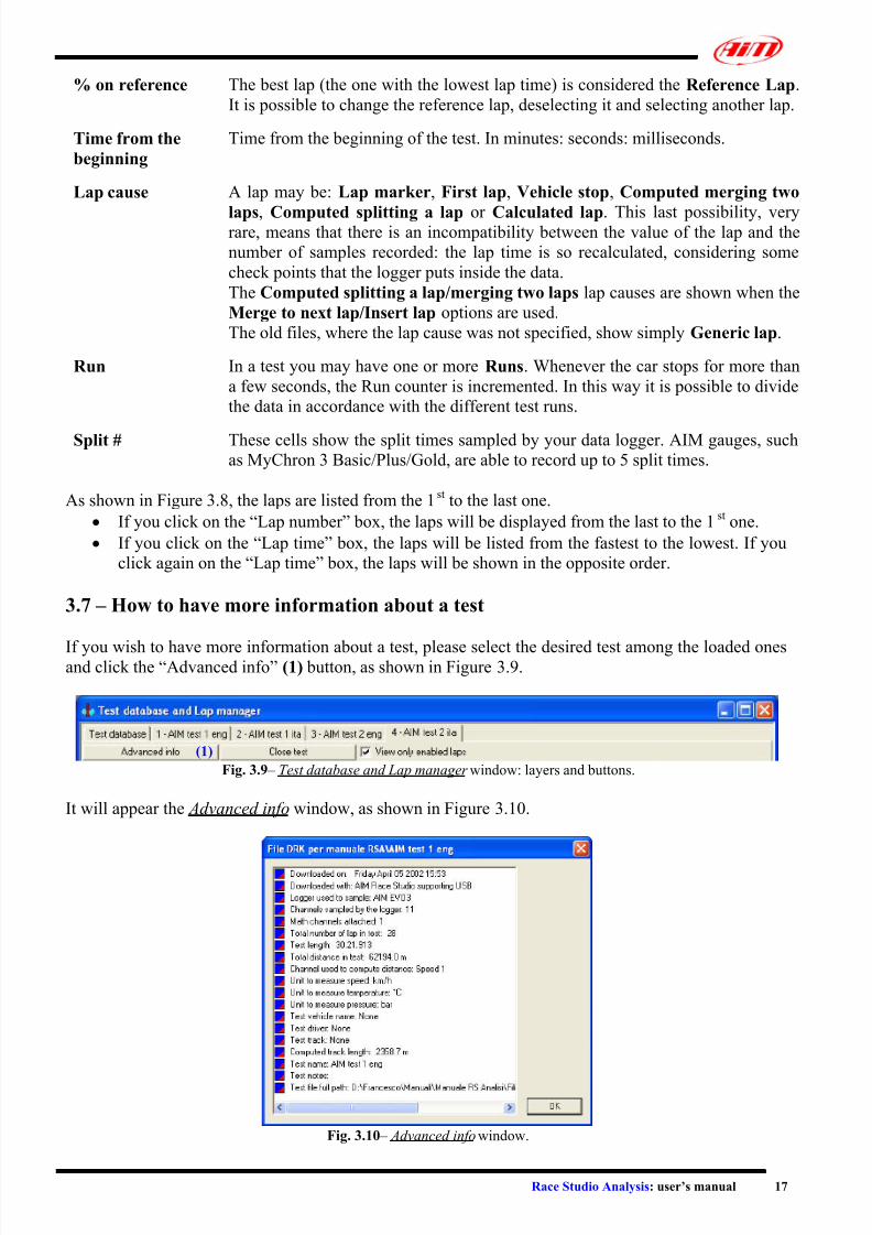
3.7 – How to have more information about a test
If you wish to have more information about a test, please select the desired test among the loaded onesand click the “Advanced info” (1) button, as shown in Figure 3.9.
Fig. 3.9 – Test database and Lap manager window: layers and buttons.
(1)
It will appear the Advanced info window, as shown in Figure 3.10.
Fig. 3.10 – Advanced info window.
7/27/2019 AIM Manual
http://slidepdf.com/reader/full/aim-manual 18/66
Race Studio Analysis: user’s manual 18
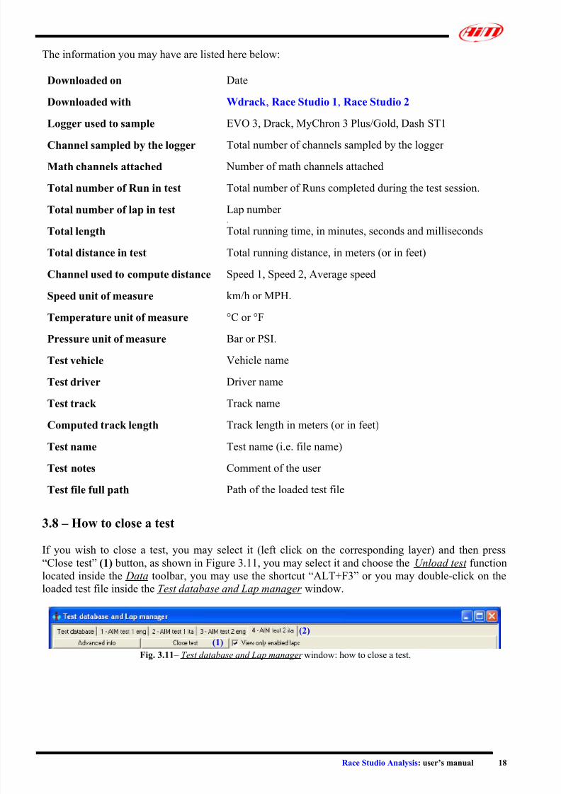
The information you may have are listed here below:
Downloaded on Date
Downloaded with Wdrack , Race Studio 1, Race Studio 2
Logger used to sample EVO 3, Drack, MyChron 3 Plus/Gold, Dash ST1
Channel sampled by the logger Total number of channels sampled by the logger
Math channels attached Number of math channels attached
Total number of Run in test Total number of Runs completed during the test session.
Total number of lap in test Lap number .
Total length Total running time, in minutes, seconds and milliseconds
Total distance in test Total running distance, in meters (or in feet)
Channel used to compute distance Speed 1, Speed 2, Average speed
Speed unit of measure km/h or MPH.
Temperature unit of measure °C or °F
Pressure unit of measure Bar or PSI.
Test vehicle Vehicle name
Test driver Driver name
Test track Track name
Computed track length Track length in meters (or in feet)
Test name Test name (i.e. file name)
Test notes Comment of the user
Test file full path Path of the loaded test file
3.8 – How to close a test
If you wish to close a test, you may select it (left click on the corresponding layer) and then press
“Close test” (1) button, as shown in Figure 3.11, you may select it and choose the Unload test function
located inside the Data toolbar, you may use the shortcut “ALT+F3” or you may double-click on the
loaded test file inside the Test database and Lap manager window.
Fig. 3.11 – Test database and Lap manager window: how to close a test.
(2)
(1)

7/27/2019 AIM Manual
http://slidepdf.com/reader/full/aim-manual 19/66
Race Studio Analysis: user’s manual 19
Chapter 4 – “How to plot a test”
4.1 – How to plot a channel vs. time
To plot a channel versus time, you may click the Plot vs. Time command, located inside the
View toolbar, you may click the proper button in the buttons toolbar or you may use the
shortcut “CTRL+F1”.
The Plot vs. time view shows the time on the horizontal axis and the channels’ recorded value on the
vertical one.
The layout of the view for overlapped graphs is shown in Figure 4.1 and described below.
Fig. 4.1 – Plot vs. time: overlapped graphs
(1)
(2)
(4)
(5)(3)
In this example graph it is reported two measured inputs (1): the engine’s RPM (red) and the vehicle
speed (black).
The graph’s abscissa axis (3) shows the time in seconds: the axis minimum is set to the default value 0
while the maximum one is set to the lap time.
The graph also reports the RPM’s (2) and the speed’s (4) axis scale (from 0 to 8000 for the RPMchannel and from 0 to 250 for the speed one). To add/remove the scale from the graph, please see
chapter 4.4.2; to modify the scale’s limits, please see chapter 4.6.1.
The vertical line (5) with a cross every time a graph is met is called “cursor”: if you click in an internal
point of the graph, the cursor will move to that point. The values of the sampled data corresponding to
that time will be shown in the Measure toolbar (see chapter 4.4).
To switch the graph from an overlapped one to a tiled or a mixed one, you may right click when the
mouse cursor is on the graph and select the desired graph type, you may choose the desired function
inside the Options toolbar or you may use the proper buttons located inside the buttons toolbar.
4.2 – How to plot a channel vs. distance
To plot a channel versus time, you may click the Plot vs. Distance command, located
inside the View toolbar, you may click the proper button in the buttons toolbar or you may
7/27/2019 AIM Manual
http://slidepdf.com/reader/full/aim-manual 20/66
Race Studio Analysis: user’s manual 20
use the shortcut “CTRL+F2”.
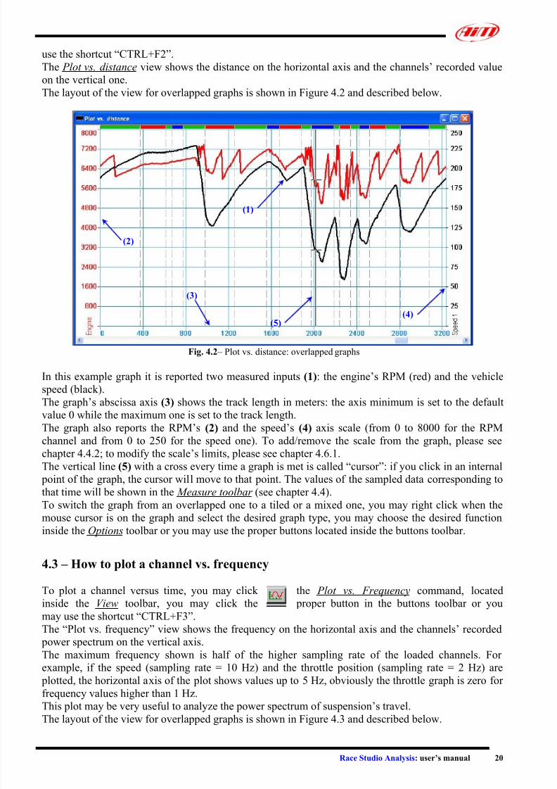
The Plot vs. distance view shows the distance on the horizontal axis and the channels’ recorded value
on the vertical one.
The layout of the view for overlapped graphs is shown in Figure 4.2 and described below.
Fig. 4.2 – Plot vs. distance: overlapped graphs
(1)
(2)
(3)
(4)(5)
In this example graph it is reported two measured inputs (1): the engine’s RPM (red) and the vehicle
speed (black).
The graph’s abscissa axis (3) shows the track length in meters: the axis minimum is set to the default
value 0 while the maximum one is set to the track length.The graph also reports the RPM’s (2) and the speed’s (4) axis scale (from 0 to 8000 for the RPM
channel and from 0 to 250 for the speed one). To add/remove the scale from the graph, please see
chapter 4.4.2; to modify the scale’s limits, please see chapter 4.6.1.
The vertical line (5) with a cross every time a graph is met is called “cursor”: if you click in an internal
point of the graph, the cursor will move to that point. The values of the sampled data corresponding to
that time will be shown in the Measure toolbar (see chapter 4.4).
To switch the graph from an overlapped one to a tiled or a mixed one, you may right click when the
mouse cursor is on the graph and select the desired graph type, you may choose the desired function
inside the Options toolbar or you may use the proper buttons located inside the buttons toolbar.
4.3 – How to plot a channel vs. frequency
To plot a channel versus time, you may click the Plot vs. Frequency command, located
inside the View toolbar, you may click the proper button in the buttons toolbar or you
may use the shortcut “CTRL+F3”.
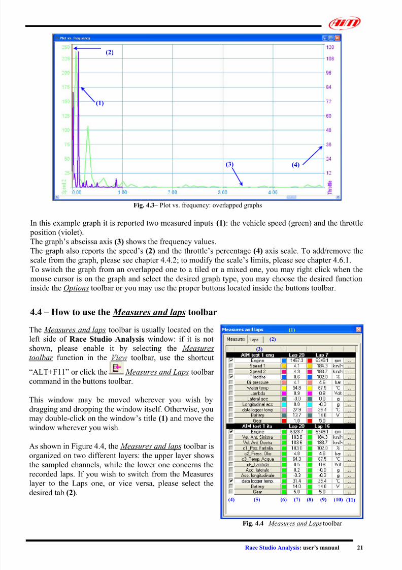
The “Plot vs. frequency” view shows the frequency on the horizontal axis and the channels’ recorded
power spectrum on the vertical axis.
The maximum frequency shown is half of the higher sampling rate of the loaded channels. For
example, if the speed (sampling rate = 10 Hz) and the throttle position (sampling rate = 2 Hz) are
plotted, the horizontal axis of the plot shows values up to 5 Hz, obviously the throttle graph is zero for
frequency values higher than 1 Hz.This plot may be very useful to analyze the power spectrum of suspension’s travel.
The layout of the view for overlapped graphs is shown in Figure 4.3 and described below.
7/27/2019 AIM Manual
http://slidepdf.com/reader/full/aim-manual 21/66
Race Studio Analysis: user’s manual 21
Fig. 4.3 – Plot vs. frequency: overlapped graphs
(2)
(1)
(3) (4)
In this example graph it is reported two measured inputs (1): the vehicle speed (green) and the throttle
position (violet).
The graph’s abscissa axis (3) shows the frequency values.
The graph also reports the speed’s (2) and the throttle’s percentage (4) axis scale. To add/remove the
scale from the graph, please see chapter 4.4.2; to modify the scale’s limits, please see chapter 4.6.1.
To switch the graph from an overlapped one to a tiled or a mixed one, you may right click when the
mouse cursor is on the graph and select the desired graph type, you may choose the desired function
inside the Options toolbar or you may use the proper buttons located inside the buttons toolbar.
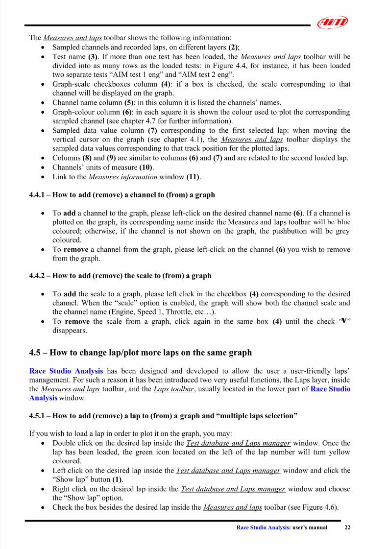
4.4 – How to use the Measures and laps toolbar
The Measures and laps toolbar is usually located on the
left side of Race Studio Analysis window: if it is not
shown, please enable it by selecting the Measures
toolbar function in the View toolbar, use the shortcut
“ALT+F11” or click the Measures and Laps toolbar
command in the buttons toolbar.
This window may be moved wherever you wish bydragging and dropping the window itself. Otherwise, you
may double-click on the window’s title (1) and move the
window wherever you wish.
As shown in Figure 4.4, the Measures and laps toolbar is
organized on two different layers: the upper layer shows
the sampled channels, while the lower one concerns the
recorded laps. If you wish to switch from the Measures
layer to the Laps one, or vice versa, please select the
desired tab (2).
Fig. 4.4 – Measures and Laps toolbar
(1)
(2)
(3)
(5)(4) (6) (7) (8) (9) (10) (11)
7/27/2019 AIM Manual
http://slidepdf.com/reader/full/aim-manual 22/66
Race Studio Analysis: user’s manual 22
The Measures and laps toolbar shows the following information:
• Sampled channels and recorded laps, on different layers (2);
• Test name (3). If more than one test has been loaded, the Measures and laps toolbar will be
divided into as many rows as the loaded tests: in Figure 4.4, for instance, it has been loaded
two separate tests “AIM test 1 eng” and “AIM test 2 eng”.
• Graph-scale checkboxes column (4): if a box is checked, the scale corresponding to that
channel will be displayed on the graph. • Channel name column (5): in this column it is listed the channels’ names.
• Graph-colour column (6): in each square it is shown the colour used to plot the corresponding
sampled channel (see chapter 4.7 for further information).
• Sampled data value column (7) corresponding to the first selected lap: when moving the
vertical cursor on the graph (see chapter 4.1), the Measures and laps toolbar displays the
sampled data values corresponding to that track position for the plotted laps.
• Columns (8) and (9) are similar to columns (6) and (7) and are related to the second loaded lap.
• Channels’ units of measure (10).
• Link to the Measures information window (11).
4.4.1 – How to add (remove) a channel to (from) a graph
• To add a channel to the graph, please left-click on the desired channel name (6). If a channel is
plotted on the graph, its corresponding name inside the Measures and laps toolbar will be blue
coloured; otherwise, if the channel is not shown on the graph, the pushbutton will be grey
coloured.
• To remove a channel from the graph, please left-click on the channel (6) you wish to remove
from the graph.
4.4.2 – How to add (remove) the scale to (from) a graph
• To add the scale to a graph, please left click in the checkbox (4) corresponding to the desired
channel. When the “scale” option is enabled, the graph will show both the channel scale and
the channel name (Engine, Speed 1, Throttle, etc…).
• To remove the scale from a graph, click again in the same box (4) until the check “V”
disappears.
4.5 – How to change lap/plot more laps on the same graph
Race Studio Analysis has been designed and developed to allow the user a user-friendly laps’
management. For such a reason it has been introduced two very useful functions, the Laps layer, inside
the Measures and laps toolbar, and the Laps toolbar , usually located in the lower part of Race Studio
Analysis window.
4.5.1 – How to add (remove) a lap to (from) a graph and “multiple laps selection”
If you wish to load a lap in order to plot it on the graph, you may:
• Double click on the desired lap inside the Test database and Laps manager window. Once the
lap has been loaded, the green icon located on the left of the lap number will turn yellow
coloured.
• Left click on the desired lap inside the Test database and Laps manager window and click the
“Show lap” button (1).• Right click on the desired lap inside the Test database and Laps manager window and choose
the “Show lap” option.
• Check the box besides the desired lap inside the Measures and laps toolbar (see Figure 4.6).
7/27/2019 AIM Manual
http://slidepdf.com/reader/full/aim-manual 23/66
Race Studio Analysis: user’s manual 23
• Right click on the desired lap number inside the Laps toolbar and choose the “Show lap”
function.
• Double click on the desired lap number inside the Laps toolbar .
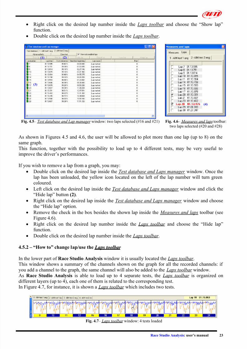
Fig. 4.5 – Test database and Lap manager window: two laps selected (#16 and #21) Fig. 4.6 – Measures and laps toolbar:two laps selected (#20 and #28)
(2)(1)
(3)
(4)
As shown in Figures 4.5 and 4.6, the user will be allowed to plot more than one lap (up to 8) on the
same graph.
This function, together with the possibility to load up to 4 different tests, may be very useful to
improve the driver’s performances.
If you wish to remove a lap from a graph, you may:
• Double click on the desired lap inside the Test database and Laps manager window. Once the
lap has been unloaded, the yellow icon located on the left of the lap number will turn green
coloured.• Left click on the desired lap inside the Test database and Laps manager window and click the
“Hide lap” button (2).
• Right click on the desired lap inside the Test database and Laps manager window and choose
the “Hide lap” option.
• Remove the check in the box besides the shown lap inside the Measures and laps toolbar (see
Figure 4.6).
• Right click on the desired lap number inside the Laps toolbar and choose the “Hide lap”
function.
• Double click on the desired lap number inside the Laps toolbar .
4.5.2 – “How to” change lap/use the Laps toolbar
In the lower part of Race Studio Analysis window it is usually located the Laps toolbar .
This window shows a summary of the channels shown on the graph for all the recorded channels: if
you add a channel to the graph, the same channel will also be added to the Laps toolbar window.
As Race Studio Analysis is able to load up to 4 separate tests, the Laps toolbar is organized on
different layers (up to 4), each one of them is related to the corresponding test.
In Figure 4.7, for instance, it is shown a Laps toolbar which includes two tests.
Fig. 4.7 – Laps toolbar window: 4 tests loaded
7/27/2019 AIM Manual
http://slidepdf.com/reader/full/aim-manual 24/66
Race Studio Analysis: user’s manual 24
The lap (laps) which is (are) shown on the graph, is (are) blue highlighted. In Figure 4.7, for instance,
laps number 18 and 21 of the “AIM test 1 eng” test are shown on the graph.
If you wish to change the lap you are watching on the graph, you may:
• Drag the blue-highlighted lap and drop it on the new lap you wish to show.
• Use the scrollbar located in the lower part of the graph (see Figure 4.1, for instance).
In the window’s right-upper corner it is shown the lap time corresponding to the lap you arehighlighting with the mouse cursor.
4.6 – How to use the Measure information window
To activate the Measure information window, you may click the Test channels command,
located inside the Modify toolbar, you may click the proper button in the buttons toolbar, you
may use the shortcut “ALT+F10”, you may click on the link to the Measure information window
inside the Measures and Laps toolbar (labelled as (11) in Figure 4.4) or you may right click on a graph
and select the “Modify test channels” function.
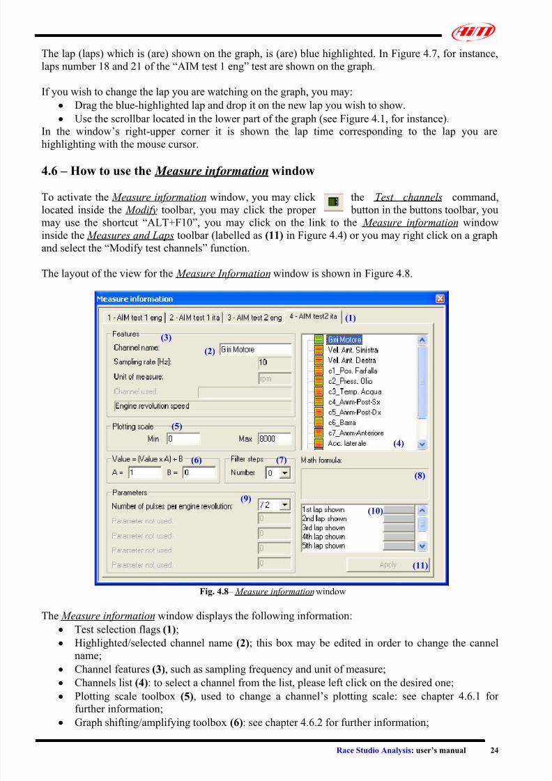
The layout of the view for the Measure Information window is shown in Figure 4.8.
Fig. 4.8 – Measure information window
(1)
(3)
(2)
(5)
(4)
(7)(6)
(8)
(9)
(10)
(11)
The Measure information window displays the following information:
• Test selection flags (1);
• Highlighted/selected channel name (2); this box may be edited in order to change the cannel
name;
• Channel features (3), such as sampling frequency and unit of measure;
• Channels list (4): to select a channel from the list, please left click on the desired one; • Plotting scale toolbox (5), used to change a channel’s plotting scale: see chapter 4.6.1 for
further information;
• Graph shifting/amplifying toolbox (6): see chapter 4.6.2 for further information;
7/27/2019 AIM Manual
http://slidepdf.com/reader/full/aim-manual 25/66
Race Studio Analysis: user’s manual 25
• Filter steps toolbox (7): used when sampled data are very noisy (see chapter 4.6.3);
• Math formula window (8): in this window it is shown the mathematic formula used to calculate
a math channel. This window can not be edited; to modify a math channel formula, please refer
to chapter 8;
• Parameters window (9): in this window it is shown the parameters used to convert the sampled
data into easily comprehensible information. It is recommended not to modify such values;
•
Shown laps colour (10): this toolbar shows 8 coloured pushbuttons which are used to set thegraph colour. Right click on the desired shown lap to enter the colour management window
(see chapter 4.7 for further information).
• The “Apply” pushbutton (11): this button is used to apply the changes to the channel’s features.
4.6.1 – How to change the plotting scale
The plotting scale toolbar, shown in Figure 4.8 as (5), is used to modify the vertical scale of a graph.
If you wish to modify the scale, please enter the desired number in the proper box: please, enter the
new scale’s minimum value inside the “Min” box, while insert the maximum value inside the “Max”
box.
It is reminded that the “Max” value must be greater than the “Min” one. If, because of a mistake, theuser sets a “Min” value greater than the “Max” one, the “Max” one will be automatically set to
“Min+1”;
These two parameters may be set in a range included between -1.000.000 and +1.000.000
4.6.2 – How to shift/amplify a graph
Race Studio Analysis allows the user to shift and amplify a sampled channel.
To shift and/or amplify a graph, please use the “Value = (Value*A)+B” option, shown in Figure 4.8 as
(6). In this math formula, A represents the “amplify factor”, while B represents the “shift factor”.
These two values are set, as a default, to 1 (amplify factor) and 0 (shift factor).
• If you wish to shift up or down a graph, please modify only the shift factor B, which may be setin a range included between -500.000 and +500.000;
• If you wish to amplify a graph, please modify the amplify factor A. The amplify factor may be
set in a range included between -1000 and +1000;
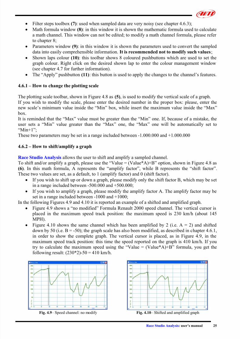
In the following Figures 4.9 and 4.10 it is reported an example of a shifted and amplified graph.
• Figure 4.9 shows a “no modified” Formula Renault 2000 speed channel. The vertical cursor is
placed in the maximum speed track position: the maximum speed is 230 km/h (about 145
MPH).
• Figure 4.10 shows the same channel which has been amplified by 2 (i.e. A = 2) and shifted
down by 50 (i.e. B = -50); the graph scale has also been modified, as described in chapter 4.6.1,
in order to show the complete graph. The vertical cursor is placed, as in Figure 4.9, in themaximum speed track position: this time the speed reported on the graph is 410 km/h. If you
try to calculate the maximum speed using the “Value = (Value*A)+B” formula, you get the
following result: (230*2)-50 = 410 km/h.
Fig. 4.9 – Speed channel: no modify Fig. 4.10 – Shifted and amplified graph

7/27/2019 AIM Manual
http://slidepdf.com/reader/full/aim-manual 26/66
Race Studio Analysis: user’s manual 26
4.6.3 – What can I do when sampled data are very noisy?
When sampled data are very noisy, for example because of the sensor’s cable has been installed near
sources of electrical interference, and you wish to analyze them, it is suggested to use the “Filter”
function, shown in Figure 4.8 as (7).
Please, enter the desired “Filter steps” number: this value may be set between 0 (no filtering) and 5
(maximum filter steps number). The higher is the filter steps number, the more are the data filtered.
For instance, in Figure 4.11 it is shown the “no filtered” lateral acceleration channel, while, in Figure
4.12, it is shown the same channel which has been “2 steps” filtered.
Fig. 4.11 – No filtered lateral acceleration Fig. 4.12 – “2 steps” filtered lateral acceleration
4.7 – How to change the graph colours
If you wish to change the graph colours, you may either left click in the graph-colour column, inside
the Measures and laps toolbar, on the coloured box corresponding to the desired lap and channel or
right click on the Laps colour toolbar inside the Measures information window.
The layout of the view for the Colours window is shown in Figure 4.13 and described below.
Fig. 4.13 – Graph colour window
(1) (2)
(3)(6)
(5)
(4)
• If the new graph colour is shown in the “Base colours” grid (1), please select it and then click
the OK button;
• Otherwise, if the colour does not appear in that grid, you may select it by clicking inside the
“rainbow” colours square (2) and you may choose the desired tonality using the proper toolbar
(3): the new colour is shown in (5). Once the correct colour has been selected, it is suggested to
add it to custom colours using the (4) button: the new colour will appear in the “Custom
colours” grid (6).
7/27/2019 AIM Manual
http://slidepdf.com/reader/full/aim-manual 27/66
Race Studio Analysis: user’s manual 27
4.8 – How to change the plot settings
To activate the Plot settings window, you may click the Plot settings command, located
inside the Options toolbar, you may click the proper button in the buttons toolbar, you may
use the shortcut “ALT+F9” or you may right-click on the graph area and chose the “Plot settings”
function.
The layout of the view for the Plot settings window is shown in Figure 4.14 and described in thefollowing chapters.
Fig. 4.14 – Plot settings window
(1)
(2)
(3)
(4)
4.8.1 – How to change the line width/cursor tags
• To change the graph line width, please select the “line width” menu, shown as (1) in Figure
4.14, and choose the desired line width among the 6 possible values: 1 (the narrowest), 2, 3, 5,
7 and 9 (the widest).
• To change the cursor tag (i.e. the horizontal line which is shown on the diagram’s vertical
cursor when a graph is met), please select the “Cursor tags” menu, shown as (2) in Figure 4.14,
and choose the desired cursor tags among the 4 possible values: none, small (default value),
large and full.
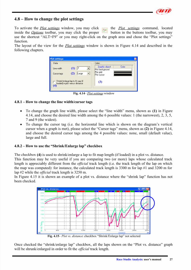
4.8.2 – How to use the “Shrink/Enlarge lap” checkbox
The checkbox (4) is used to shrink/enlarge a lap to fit map length (if loaded) in a plot vs. distance.
This function may be very useful if you are comparing two (or more) laps whose calculated track
length is appreciably different from the official track length (i.e. the track length of the lap on which
the map was computed): for instance, the calculated track length is 3300 m for lap #1 and 3200 m for
lap #2 while the official track length is 3250 m.
In Figure 4.15 it is shown an example of a plot vs. distance where the “shrink lap” function has not
been checked.
Fig. 4.15 – Plot vs. distance: checkbox “Shrink/Enlarge lap” not selected
Once checked the “shrink/enlarge lap” checkbox, all the laps shown on the “Plot vs. distance” graph
will be shrunk/enlarged in order to fit the official track length.
7/27/2019 AIM Manual
http://slidepdf.com/reader/full/aim-manual 28/66
Race Studio Analysis: user’s manual 28
4.8.3 – How to change the background (grid/cursor) colour
• To change the background (grid/cursor) colour, please select the “Colours” menu, shown as (3)
in Figure 4.14, choose the desired graphic object you wish to change the colour and right click
on the colour box. It will appear the “Colour window” previously described in chapter 4.7:
please, refer to this chapter for further information.
4.9 – How to Zoom in/Zoom out a graph
The zoom function expands the horizontal axis of the plot.
To activate the Zoom function, you may click the Zoom enable command, located inside the
Options toolbar, you may click the proper button in the buttons toolbar, you may use the
shortcut “SHIFT+F9” or you may click the right button when the mouse cursor is on a graph and select
the Zoom enable function.
Once the zoom has been enabled, the mouse cursor will turn into a circle: to “zoom in” a graph, please
click the left button on the first point of the “to be zoomed” area, then keep the mouse button pushed
and un-click it on the last point of the “to be zoomed” area.
To disable the Zoom function, you may click the Zoom disable command, located inside the
Options toolbar, you may click the proper button in the buttons toolbar, you may use the
shortcut “SHIFT+F10” or you may click the right button when the mouse cursor is on a graph and
select the Zoom disable function.
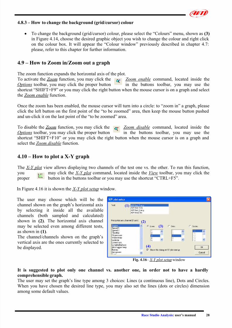
4.10 – How to plot a X-Y graph
The X-Y plot view allows displaying two channels of the test one vs. the other. To run this function,
you may click the X-Y plot command, located inside the View toolbar, you may click the proper button in the buttons toolbar or you may use the shortcut “CTRL+F5”.
In Figure 4.16 it is shown the X-Y plot setup window.
The user may choose which will be the
channel shown on the graph’s horizontal axis
by selecting it inside all the available
channels (both sampled and calculated)
shown in (2). The horizontal axis channel
may be selected even among different tests,
as shown in (1).The channel/channels shown on the graph’s
vertical axis are the ones currently selected to
be displayed.
Fig. 4.16 – X-Y plot setup window
(1)
(2)
(3)
(4)
It is suggested to plot only one channel vs. another one, in order not to have a hardly
comprehensible graph.
The user may set the graph’s line type among 3 choices: Lines (a continuous line), Dots and Circles.
When you have chosen the desired line type, you may also set the lines (dots or circles) dimensionamong some default values.

7/27/2019 AIM Manual
http://slidepdf.com/reader/full/aim-manual 29/66
Race Studio Analysis: user’s manual 29
If the checkbox (4) is enabled, the window shown in Figure 4.16 will be shown each time the X-Y plot
is started. Otherwise, if the checkbox is disabled, it will be shown the X-Y plot; right click inside the
graph area to activate the X-Y Plot setup window.
The X-Y plot has some differences from the other plots. In fact it has not the vertical cursor and the
zooming functions are not defined.
This graph can become very useful to analyze, for instance, the lateral acceleration (on the vertical
axis) vs. the lateral one (on the horizontal axis), as shown in Figure 4.17.
Fig. 4.17 – X-Y plot : longitudinal acceleration (horizontal axis) vs. lateral acceleration (vertical axis)
4.11 – How to change graph type
The Graphs type option allows changing the style of graphs’ view from “Tiled” to “Overlapped” or
“Mixed” and vice versa.
To run this function, you may click the desired graph type inside the Options toolbar, you may click
the right button when the mouse cursor is on a graph and select the desired graph type or you may
click the proper button inside the Button toolbar , as shown below:
Overlapped graphs;
Mixed graphs;
Tiled graphs.
4.12 – Laps management
The Test database and Lap manager window, shown in Figure 4.18, includes some buttons which are
very useful for the laps management.
Fig. 4.18 – Test database and Lap manager window: laps management functions
(1)
(5)(2) (3) (4)

7/27/2019 AIM Manual
http://slidepdf.com/reader/full/aim-manual 30/66
Race Studio Analysis: user’s manual 30
4.12.1 – How to enable (disable) a lap
When a new test is loaded, all the laps included inside that test will be enabled. When a lap is enabled,
it is show both inside the Laps toolbar and inside the Measures and laps toolbar. Otherwise, if the lap
is disabled, it will not be shown in the toolbars and the user will not be allowed to plot it on the graph.
• If you wish to disable a lap, you may select the desired one and press button “Disable lap” (3),
you may right click on the desired lap inside the Test database and lap manager window and
choose the “Disable” function or you may right click on the desired lap inside the Laps toolbar
and choose the “Disable” function.
• If you wish to enable a disabled lap, you may select it and press button “Enable lap” (2) or you
may right click on the desired lap inside the Test database and lap manager window and
choose the “Enable” function.
If you wish to remove the disabled laps from the Test database and Laps manager window, you may
check the checkbox “View only enabled laps” (1).
It is suggested to disable all the “First laps” and “Vehicle stop laps”.
4.12.2 – How to insert a lap
If the lap receiver has not been able to capture a lap (because of an incorrect installation or technical
problems), the Test database and Lap manager window will show a lap (and its corresponding lap
time) obtained by merging two consecutive laps. If you have manually elapsed the lap time, or you
may read the lap time from the official times list, Race Studio Analysis will allow you to split the lap
into two separate laps.
Select the lap you wish to split (double click on the lap number) and press button “Insert lap” (4). The
Insert lap time window is shown in Figure 4.19 and described below.
Fig. 4.19 – Insert lap time window
Please insert the lap time (minutes, seconds and milliseconds) inside the three boxes. Once the lap time
has been set, press button “OK”. Inside the Test database and Lap manager window it will appear a
new lap labelled, inside the “Lap cause” column, as “Computed splitting a lap”.
4.12.3 – How to merge a lap to the next one
If you wish to merge a lap to the next one, please select the desired lap and press button “Merge lap”
(5). Inside the Test database and Lap manager window it will appear a new lap labelled, inside the
“Lap cause” column, as “Computed merging two laps”.
7/27/2019 AIM Manual
http://slidepdf.com/reader/full/aim-manual 31/66
Race Studio Analysis: user’s manual 31
Chapter 5 – “How to create a track map”
5.1 – Introduction
Race Studio Analysis software allows calculating the track map directly from the recorded data. The
map commands allow a full management of the track maps (creating a new map, modifying and
loading an existing one, using the map database)
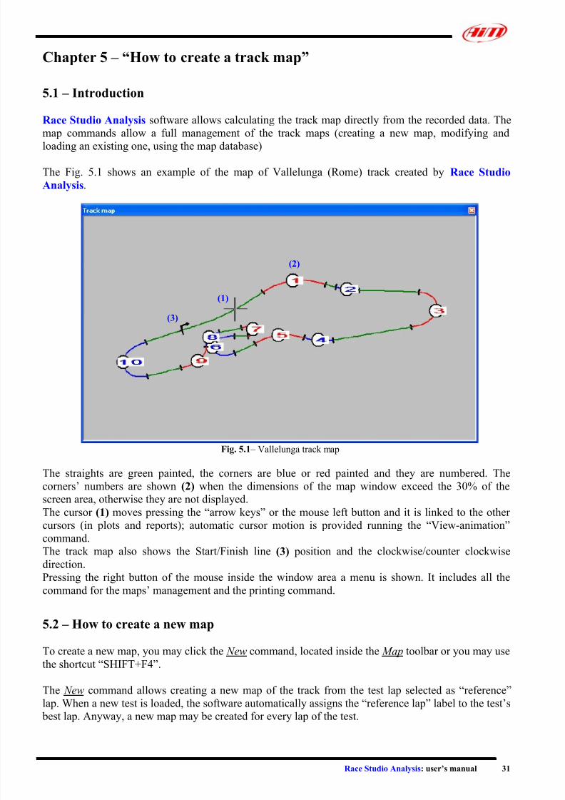
The Fig. 5.1 shows an example of the map of Vallelunga (Rome) track created by Race Studio
Analysis.
Fig. 5.1 – Vallelunga track map
(2)
(1)
(3)
The straights are green painted, the corners are blue or red painted and they are numbered. The
corners’ numbers are shown (2) when the dimensions of the map window exceed the 30% of the
screen area, otherwise they are not displayed.
The cursor (1) moves pressing the “arrow keys” or the mouse left button and it is linked to the other
cursors (in plots and reports); automatic cursor motion is provided running the “View-animation”
command.
The track map also shows the Start/Finish line (3) position and the clockwise/counter clockwise
direction.Pressing the right button of the mouse inside the window area a menu is shown. It includes all the
command for the maps’ management and the printing command.
5.2 – How to create a new map
To create a new map, you may click the New command, located inside the Map toolbar or you may use
the shortcut “SHIFT+F4”.
The New command allows creating a new map of the track from the test lap selected as “reference”
lap. When a new test is loaded, the software automatically assigns the “reference lap” label to the test’s best lap. Anyway, a new map may be created for every lap of the test.
7/27/2019 AIM Manual
http://slidepdf.com/reader/full/aim-manual 32/66
Race Studio Analysis: user’s manual 32
For the creation of a map some channels have to be recorded, they differ because of the vehicle in use.
• For a four wheels vehicle the reference speed channel and the lateral acceleration channels are
necessary
• For a two wheels vehicle the reference speed channel and the gyroscope channels are needed.
If these channels are not available, it WILL NOT BE POSSIBLE to calculate the track map.
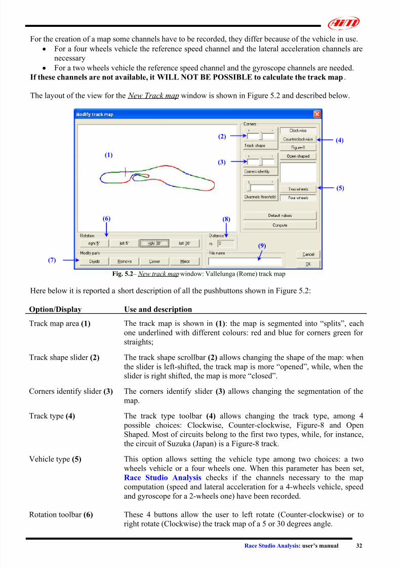
The layout of the view for the New Track map window is shown in Figure 5.2 and described below.
Fig. 5.2 – New track map window: Vallelunga (Rome) track map
(2)(4)
(1)(3)
(5)
(6) (8)
(9)
(7)
Here below it is reported a short description of all the pushbuttons shown in Figure 5.2:
Option/Display Use and description
Track map area (1) The track map is shown in (1): the map is segmented into “splits”, each
one underlined with different colours: red and blue for corners green for
straights;
Track shape slider (2) The track shape scrollbar (2) allows changing the shape of the map: when
the slider is left-shifted, the track map is more “opened”, while, when the
slider is right shifted, the map is more “closed”.
Corners identify slider (3) The corners identify slider (3) allows changing the segmentation of the
map.
Track type (4) The track type toolbar (4) allows changing the track type, among 4
possible choices: Clockwise, Counter-clockwise, Figure-8 and Open
Shaped. Most of circuits belong to the first two types, while, for instance,
the circuit of Suzuka (Japan) is a Figure-8 track.
Vehicle type (5) This option allows setting the vehicle type among two choices: a two
wheels vehicle or a four wheels one. When this parameter has been set,
Race Studio Analysis checks if the channels necessary to the map
computation (speed and lateral acceleration for a 4-wheels vehicle, speed
and gyroscope for a 2-wheels one) have been recorded.
Rotation toolbar (6) These 4 buttons allow the user to left rotate (Counter-clockwise) or to
right rotate (Clockwise) the track map of a 5 or 30 degrees angle.

7/27/2019 AIM Manual
http://slidepdf.com/reader/full/aim-manual 33/66
Race Studio Analysis: user’s manual 33
Modify parts toolbar (7) This toolbar allows modifying the track map. In particular, it is possible
to:
• Divide a split into two separate splits: the new split starts at the
cursor position and finishes at the end of the current split. Each
modified part is created as a corner;
• Remove an intermediate split;
• Change a circuit part from corner to straight and vice versa.WARNING: it is not possible to have two consecutive straights;
• Mirror the track map.
Distance (8) When clicking on the track map, in this box it is shown the distance
calculated from the Start/Finish line.
File name (9) If you wish to save the map, before clicking the OK button, it is necessary
to insert the track name inside the (9) box; the maximum name input
length is 40 characters.
Otherwise, if you wish to exit without saving, please press button
“Cancel”.
When the map has been created, if you wish to see it on your PC’s monitor, you may click the Show
track map command, located inside the Map toolbar, you may click the proper button in the
buttons toolbar, you may use the shortcut “SHIFT+F1” or you may click the right button
when the mouse cursor is on a graph and select the Track map function.
5.3 – Track map creation troubleshooting
In this chapter it will be described the solutions to the most frequently asked questions concerning the
map creation problems.
• If, when trying to create a new track map, it appears the warning message “Invalid data to
compute track map”, please select a “good” lap, labelled as “Lap marker” in the Test database
and Lap manager window (see Figure 3.8). It is reminded to select the new lap and then, before
retrying to create the map, to deselect the lap previously used.
• It is recommended to select a lap without many skids and sudden braking.
• Verify that you have set the correct vehicle type (i.e. 2 or 4 wheels) in the New track map
window (see Figure 5.2).
• Verify that speed and acceleration (4 wheels vehicle) or speed and gyroscope (2 wheels
vehicle) channels are sensible:
o The speed must be greater than 0 and must not have high or low peaks. In case the
speed channel is very noisy and you have recorded 2 speed inputs (for instance the 2
front wheels speed), you may change the reference speed channel, as explained in
chapter 5.4.
o The lateral acceleration must be near 0 on the straight line;
• If lateral acceleration in the straight line in not near 0, it is probable that the lateral
accelerometer has not been calibrated. In this case, it is possible to calculate the map shifting
up or down the lateral acceleration graph, as here below explained:o Plot the lateral acceleration vs. time;
o Place the vertical cursor on the graph in a position corresponding to a straight: in this
track position the lateral acceleration should be 0;
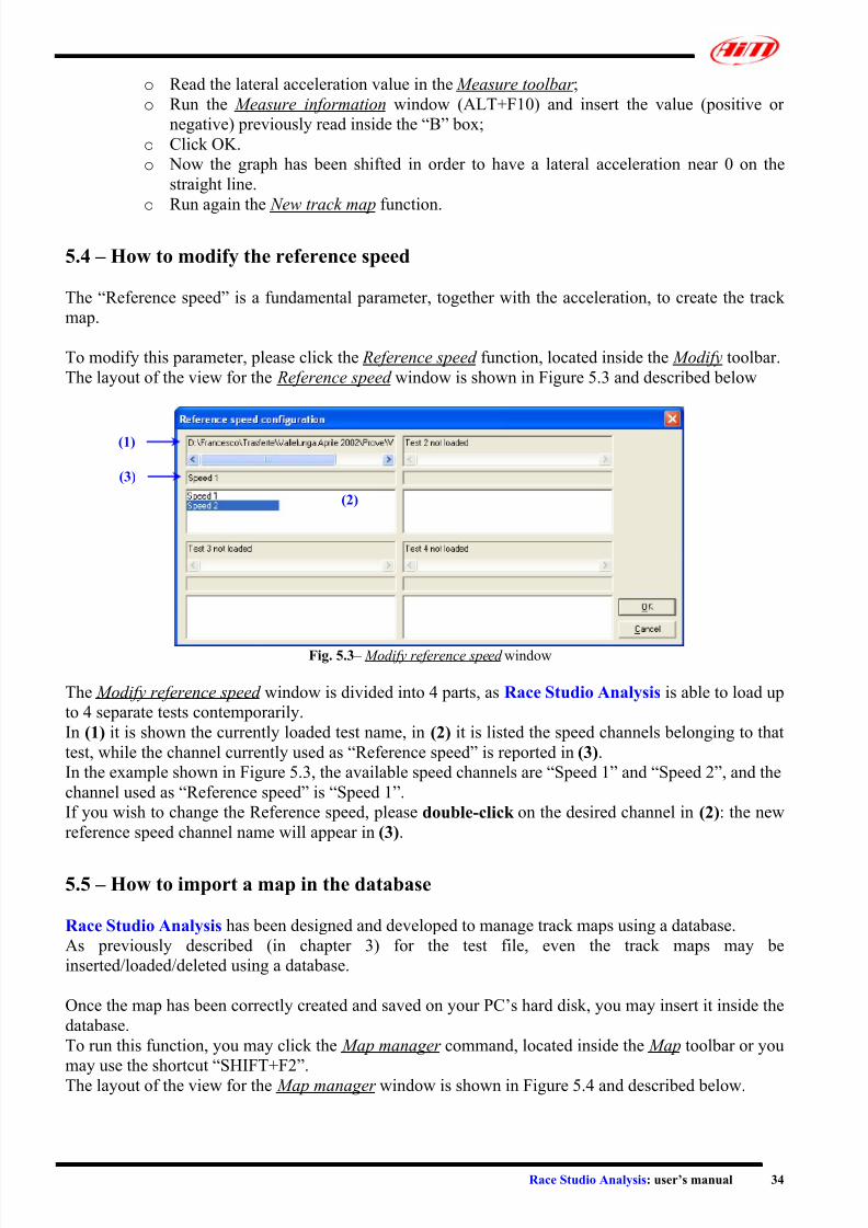
7/27/2019 AIM Manual
http://slidepdf.com/reader/full/aim-manual 34/66
Race Studio Analysis: user’s manual 34
o Read the lateral acceleration value in the Measure toolbar ;
o Run the Measure information window (ALT+F10) and insert the value (positive or
negative) previously read inside the “B” box;
o Click OK.
o Now the graph has been shifted in order to have a lateral acceleration near 0 on the
straight line.
o Run again the New track map function.
5.4 – How to modify the reference speed
The “Reference speed” is a fundamental parameter, together with the acceleration, to create the track
map.
To modify this parameter, please click the Reference speed function, located inside the Modify toolbar.
The layout of the view for the Reference speed window is shown in Figure 5.3 and described below
Fig. 5.3 – Modify reference speed window
(1)
(3)
(2)
The Modify reference speed window is divided into 4 parts, as Race Studio Analysis is able to load up
to 4 separate tests contemporarily.
In (1) it is shown the currently loaded test name, in (2) it is listed the speed channels belonging to that
test, while the channel currently used as “Reference speed” is reported in (3).
In the example shown in Figure 5.3, the available speed channels are “Speed 1” and “Speed 2”, and the
channel used as “Reference speed” is “Speed 1”.
If you wish to change the Reference speed, please double-click on the desired channel in (2): the new
reference speed channel name will appear in (3).
5.5 – How to import a map in the database
Race Studio Analysis has been designed and developed to manage track maps using a database.
As previously described (in chapter 3) for the test file, even the track maps may be
inserted/loaded/deleted using a database.
Once the map has been correctly created and saved on your PC’s hard disk, you may insert it inside the
database.
To run this function, you may click the Map manager command, located inside the Map toolbar or you
may use the shortcut “SHIFT+F2”.
The layout of the view for the Map manager window is shown in Figure 5.4 and described below.
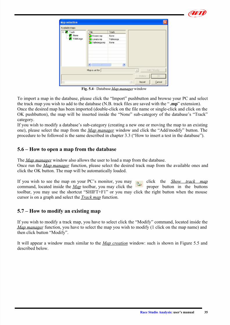
7/27/2019 AIM Manual
http://slidepdf.com/reader/full/aim-manual 35/66
Race Studio Analysis: user’s manual 35
Fig. 5.4 – Database Map manager window
To import a map in the database, please click the “Import” pushbutton and browse your PC and select
the track map you wish to add to the database (N.B. track files are saved with the “ .mp” extension).
Once the desired map has been imported (double-click on the file name or single-click and click on the
OK pushbutton), the map will be inserted inside the “None” sub-category of the database’s “Track”category.
If you wish to modify a database’s sub-category (creating a new one or moving the map to an existing
one), please select the map from the Map manager window and click the “Add/modify” button. The
procedure to be followed is the same described in chapter 3.3 (“How to insert a test in the database”).
5.6 – How to open a map from the database
The Map manager window also allows the user to load a map from the database.
Once run the Map manager function, please select the desired track map from the available ones and
click the OK button. The map will be automatically loaded.
If you wish to see the map on your PC’s monitor, you may click the Show track map
command, located inside the Map toolbar, you may click the proper button in the buttons
toolbar, you may use the shortcut “SHIFT+F1” or you may click the right button when the mouse
cursor is on a graph and select the Track map function.
5.7 – How to modify an existing map
If you wish to modify a track map, you have to select click the “Modify” command, located inside the
Map manager function, you have to select the map you wish to modify (1 click on the map name) andthen click button “Modify”.
It will appear a window much similar to the Map creation window: such is shown in Figure 5.5 and
described below.
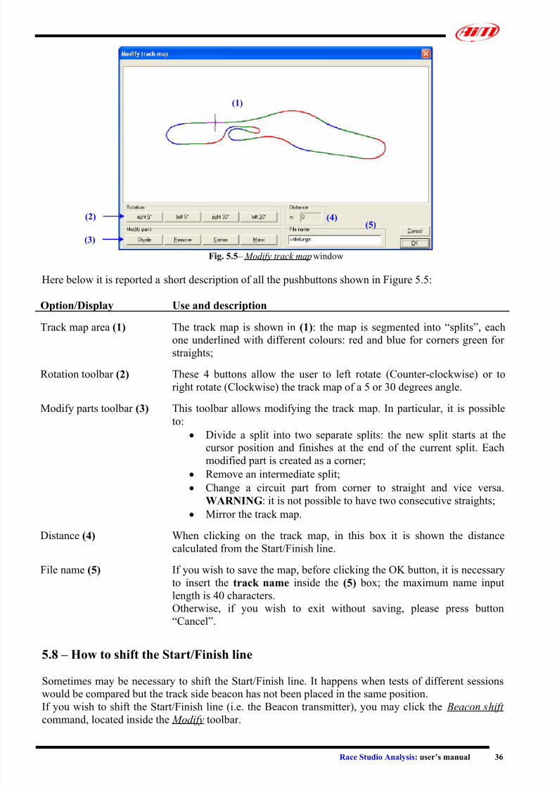
7/27/2019 AIM Manual
http://slidepdf.com/reader/full/aim-manual 36/66
Race Studio Analysis: user’s manual 36
Fig. 5.5 – Modify track map window
(1)
(2) (4)(5)
(3)
Here below it is reported a short description of all the pushbuttons shown in Figure 5.5:
Option/Display Use and description
Track map area (1) The track map is shown in (1): the map is segmented into “splits”, each
one underlined with different colours: red and blue for corners green for
straights;
Rotation toolbar (2) These 4 buttons allow the user to left rotate (Counter-clockwise) or to
right rotate (Clockwise) the track map of a 5 or 30 degrees angle.
Modify parts toolbar (3) This toolbar allows modifying the track map. In particular, it is possibleto:
• Divide a split into two separate splits: the new split starts at the
cursor position and finishes at the end of the current split. Each
modified part is created as a corner;
• Remove an intermediate split;
• Change a circuit part from corner to straight and vice versa.
WARNING: it is not possible to have two consecutive straights;
• Mirror the track map.
Distance (4) When clicking on the track map, in this box it is shown the distance
calculated from the Start/Finish line.
File name (5) If you wish to save the map, before clicking the OK button, it is necessary
to insert the track name inside the (5) box; the maximum name input
length is 40 characters.
Otherwise, if you wish to exit without saving, please press button
“Cancel”.
5.8 – How to shift the Start/Finish line
Sometimes may be necessary to shift the Start/Finish line. It happens when tests of different sessions
would be compared but the track side beacon has not been placed in the same position.If you wish to shift the Start/Finish line (i.e. the Beacon transmitter), you may click the Beacon shift
command, located inside the Modify toolbar.

7/27/2019 AIM Manual
http://slidepdf.com/reader/full/aim-manual 37/66
Race Studio Analysis: user’s manual 37
NOTES: it is reminded that the Beacon shift option may be used only if the track map has been
created / loaded.
The layout of the view for the Beacon shift window is shown in Figure 5.6 and described below.
Fig. 5.6 – Beacon shift window
(3)(2)(1)
(4)
This function allows the user to set the distance between the actual Beacon (i.e. the track start/finish
line) and the recorded one (i.e. the position where you installed your Beacon transmitter).
To shift the Start/Finish line, please enter the distance between the actual Beacon and the recorded one
in (1) and, in (2), set if the actual Beacon was installed before or after the recorded one.
Click the “Check” button (3) to verify if the values you set are correct. It is reminded that the Beacon
may be shifted up to 500 m.
The “Reset” button (4) will allow you to cancel the changes.
To exit saving and applying the changes press button “OK”; to exit discarding the changes press button
“Cancel”.

7/27/2019 AIM Manual
http://slidepdf.com/reader/full/aim-manual 38/66
Race Studio Analysis: user’s manual 38
Chapter 6 – “How to get further information from sampled data”
6.1 – Introduction
The functions here below described will allow the user to get further information from sampled data,
such as Histogram graphs, Lap/Split times analysis. These functions will also allow the user to
calculate the car (bike, kart) acceleration (picking up of speed) times.
If correctly used, these commands will allow the driver to improve both his performances and the
vehicle setup.
6.2 – How to plot a Histogram graph
The “Histogram” command allows displaying the histogram of the channel in evidence. To run this
function, you may click the Histogram command, located inside the View toolbar, you
may click the proper button in the buttons toolbar or you may use the shortcut “CTRL+F8”.
The histogram shows the distribution of data into individual ranges (1).
The example of a histogram for the “Engine” channel is shown in Figure 6.1.
Fig. 6.1 – Histogram graph: engine’s RPM and speed
(1)
(2)
(3)
The histogram may show either percentage of data samples falling into each range (as shown in Figure
6.1) or total time spent in the range. The percentage or time may be changed using the mouse right
button menu or the Percentage/Time function, located inside the Options toolbar.
On the left side of the window the vertical axis (2) shows the data range. The zero – full scale interval
of the channel is divided in a configurable number of bins: if you want to change the scale interval of
the channel, select the Change bins function by right-clicking on the drawing area. The number of bins
may be set in a range included between 3 and 50.
The horizontal axis (3) shows the percentage (or time) for each range.
Pressing the right button of the mouse, when the mouse cursor is inside the histogram drawing area, a
menu is displayed. It includes the most important commands for the “Histogram” management.
The printing function is available.

7/27/2019 AIM Manual
http://slidepdf.com/reader/full/aim-manual 39/66
Race Studio Analysis: user’s manual 39
6.3 – How to use the Lap Times analysis
The “Lap times” command allows displaying a histogram graph of the laps belonging to the loaded
tests.
To run this function, you may click the Lap times command, located inside the View toolbar or you
may use the shortcut “CTRL+F7”.
An example of a Lap Times analysis graph is shown in Figure 6.2 and described below.
Fig. 6.2 – Lap times analysis: 2 tiled graphs
(3)
(5)(2)(4)
(3)
(1)
The Lap Times report window is divided into two separate parts: on the left (1) it is shown the loadedtests and the tests’ laps, while, on the right, it is shown a histogram graph reporting the lap times.
When more than one test has been loaded, the histograms are displayed on a tiled graph, as reported in
Figure 6.2 (2 tests loaded).
The left side of the graph may be hidden by clicking the vertical bar (2), in order to amplify the
plotting area of the histogram graph.
The lap times are shown as red histograms: the best lap for each test is shown with a blue histogram
(5). When you move the mouse cursor on a lap, the histogram turns pink coloured and the
corresponding lap time is shown in the graph’s upper left corner (3).
The Lap times function also shows a green horizontal bar (4), which represents the test’s average time.
6.4 – How to use the Split Times analysis
This report calculates the time necessary to run along each part of the active map (corners and straights
are the track parts) for each lap. The program, during the map creation, calculates the number and the
length of the parts.
The Split times function allows the user to make both a numerical and a graphical compare between
the split times.
To run this function, you may click the Split times command, located inside the View
toolbar, you may click the proper button in the buttons toolbar or you may use the shortcut
“CTRL+F6”.An example of a Split Times analysis graph (numerical compare) is shown in Figure 6.3 and described
below.

7/27/2019 AIM Manual
http://slidepdf.com/reader/full/aim-manual 40/66
Race Studio Analysis: user’s manual 40
Fig. 6.3 – Split times analysis: numerical compare
(1)
(5)(2) (6)
(3) (4)
Each column represents a segment; colours at the top of the column are so labelled: red and blue for
corners and green for straights.The Split report window is organized on different layers and you may switch among them using the
tab (1). The first layer is called Test compare and is used to compare 2 or more tests (up to 4), while
the other ones are used to switch among the loaded tests (up to 4).
Buttons Numerical (5) and Graphical (6) are used to select the compare type: in Figure 6.3 it is shown
the Numerical compare, while the Graphical one is shown in Figure 6.5.
The first column (3) on the left shows the loaded test name, the second one shows the lap number,
columns from the third to the last but one report the split times and the last column shows the lap time.
Button Export to Excel (2) is used to export the split times in a format compatible with Microsoft
Excel ™.
The Numerical split times window is also divided into horizontal fields.
• The first one, starting from the top of the window, shows the “Absolute split times”: the best
lap time within each lap is blue highlighted, while the best lap’s split times are red coloured. In
the lower part of the “Absolute split times” field it is shown some statistics values, such as the
minimum/maximum/average value and the standard deviation.
• The second one reports the “Theoretical best lap”, which assembles the best lap that could have
been run in the session. Segments which make up the theoretical best lap are red painted;
• The “Best rolling lap” represents the fastest lap done irrespective of the location of the beacon;
• The last field shows the “Split time differences from the best lap within test”: a negative valuemeans that the track segment has been run in a time lower than the corresponding split time of
the best lap.
If button Histogram (4) is pressed, the split times shown in the corresponding column will be
displayed both on a numerical and graphical view.
The graphical view consists in a blue histogram. The histogram’s length is directly proportional to the
split time: the higher it is the split time, the longer it is the histogram.
In Figure 6.4 it is shown the numerical compare with 3 histograms (concerning curves number 2, 3 and
4).

7/27/2019 AIM Manual
http://slidepdf.com/reader/full/aim-manual 41/66
Race Studio Analysis: user’s manual 41
Fig. 6.4 – Split times analysis: numerical compare, Histograms
The Split times analysis is able to manage numerical and graphical compare between laps belonging to
separate tests.
To switch from the numerical view to the graphical one, please click button Graphical (6) on the top
side of Figure 6.3.
An example of a Split Times graphical compare is shown in Figure 6.5 and described below.
Fig. 6.5 – Split times analysis: graphical compare
(1)
(2)
(5)
(6)
(3) (4)
The graphical compare window is divided into two separate parts: on the left (4) it is shown the test
laps (lap number and lap time) while, on the right, it is reported the graphical compare between the
selected laps.
To select a lap, please click it: the selected lap (4) will turn blue coloured. To unselect a lap, re-click
on the lap.
It is reminded that the graphical compare is able to manage up to 8 laps contemporarily.
As the Numerical compare, even the Graphical one is organized on different layers: you may switch
among them using the tabs (1). The Export to Excel function (2) is disabled when running theGraphical compare.
Left click on the coloured squares (3) if you wish to change the histograms’ colour.

7/27/2019 AIM Manual
http://slidepdf.com/reader/full/aim-manual 42/66
Race Studio Analysis: user’s manual 42
On the right of the Graphical compare window it is shown:
• The test name, the lap number, the lap time and the split time (5) are shown in the upper part.
The best split time is also labelled as “Best split”, while the other ones are labelled as
“Slower”.
• The histograms (6) in the lower part of the right side of the Graphical compare window are
directly proportional to the split time. The best split time is shown on the foreground, while theother ones are shown on the background.
6.5 – How to use the Channels report
The Channels report function allows the user to visualize a complete summary both of sampled data
and of recorded laps.
In particular, this function allows the user to visualize, for each sampled data, the maximum/minimum
value, the time and the distance (from the start/finish line) corresponding to the maximum/minimum
value and the average value.
To run this function, you may select the Channels report command inside the View toolbar or
you may use the proper pushbutton inside the Buttons toolbar . An example of the channels
report window for a sample test is shown in Figure 6.6.
Fig. 6.6 – Channels report window: configuration layer
(1)
(8)(7)
(4)(3)
(2)
(5)
(6)(9)
The Channels report window is organized on as many layers as the number of the loaded tests. Please,
select the desired test clicking on the proper flag (1).
Place a check in the checkboxes (6) corresponding to the desired channels and features (max/min
value, etc…). Once selected the desired features, please enter the setting name inside box (2) and press
button “Save” (3) to save the new setting. The setting will appear inside the available sets list (5).
If you wish to delete an undesired setting, please select it and press button “Delete” (4).
The Export to Excel function (8) is available only when button Set is not pressed.
Buttons Import and Export (9) are used to import / export the desired setting. These settings will be
saved in the hard disk in a “.CRP” file.
Now you may press the “Set” button (7) in order to switch the Channels report window from the“configuration” layer to the “graphical visualization” one, shown in Figure 6.7.

7/27/2019 AIM Manual
http://slidepdf.com/reader/full/aim-manual 43/66
Race Studio Analysis: user’s manual 43
Fig. 6.7 – Channels report window: graphical visualization layer
Inside this window it is shown the desired values and input channels corresponding to the active laps.
As shown in Figure 6.7, it is reminded that the best lap (lap #22) is written in bold character and the
overall best input channels’ values are white highlighted.
If button Histo is pressed, the values shown in the corresponding column will be displayed both on a
numerical and graphical view.
The graphical view consists in a blue histogram. The histogram’s length is directly proportional to the
channel’s value: the higher it is this value, the longer it is the histogram (see Figure 6.8 for further
information).
Fig. 6.8 – Channels report window: graphical visualization layer – button Histo pressed
The “Test compare” button is used to make a comparison between the loaded tests. It is reminded that,
in order to make this comparison, the tests must have the settings (i.e. you have to set the same setting
among the “available settings list” for all the loaded tests).
6.6 – How to use the Acceleration report
The “Acceleration report” allows calculating the time needed to reach up to 4 different speed values.
This view is very useful for the evaluation of the acceleration of the vehicle.
To run this function, you may click the Acceleration view command, located inside the View toolbar or
you may right-click on the graph area when you plot a channel vs. time.

7/27/2019 AIM Manual
http://slidepdf.com/reader/full/aim-manual 44/66
Race Studio Analysis: user’s manual 44
A correct procedure for the use of this function is described here below:
1. Be sure the Plot vs. time has been run and the speed channel is displayed.
2. Put the cursor at the beginning of the section you would like to analyse: in Figure 6.10, the
cursor has been placed in a low-peak speed position.
3. Run the “View-Acceleration report” command from the analysis menu or the “Acceleration
report” command from the menu shown pressing the right button of the mouse in the “Plot vs.
time” window. The dialog window shown in Figure 6.9 is displayed.
4. In the dialog window input the speed threshold values (maximum 4), when finished press the
“Compute” button (2). The program calculates the acceleration time and shows them in (6).
Fig. 6.9 – Acceleration report window Fig. 6.10 – Vehicle speed graph
(1)
(8)
(2)
(3)
(4)(7)
(5)(6)
Option/Display Use
Generals (1) In this field the name of the test and the number of the lap are shown.
Moreover the maximum speed (3) in the lap is shown.
Acceleration times:
Speed and Time
Input in column (5) the speed threshold values.
(4) shows the speed at the cursor position (7).
It is reminded that it is not possible to set a threshold value greater both than
the maximum speed (3) and than the nearest speed high peak (8), and that the
values set in (5) must be greater than (4).
Calculated time to reach the threshold values from the previous step will be
shown in (6).
Exit Choose this command to exit the dialog window.
Compute (2) Choose this command to start the computation of the time values.
Print Choose this command to print the report.
6.7 – How to use the Track report
The “Track report” view command allows showing the map of the track painted with different colours
depending on the values of a channel.
The cursor motion around the track map may be performed manually (using some buttons on the view
or clicking the mouse button in the desired track position) or automatically (selecting the Animation
command). The cursor is linked to all the other ones, in plots or reports.
To run this function, please select the Track report function, located inside the View menu, or use the
shortcut “CTRL+F12”.
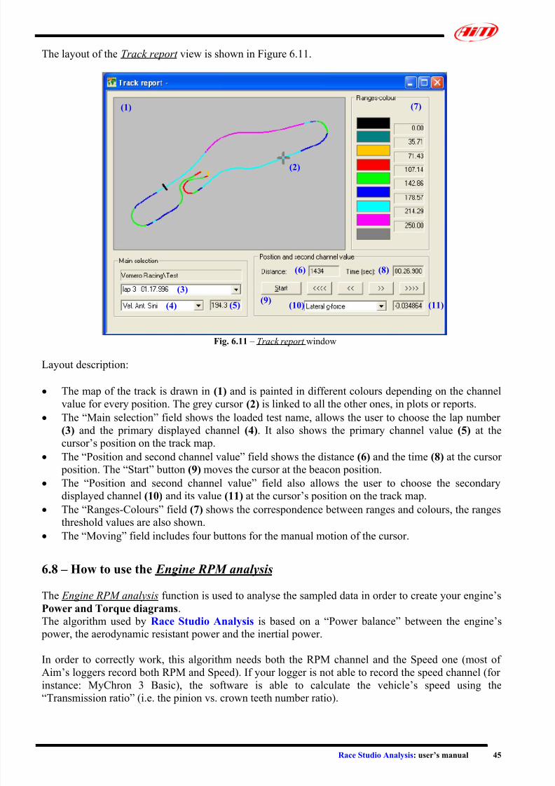
7/27/2019 AIM Manual
http://slidepdf.com/reader/full/aim-manual 45/66
Race Studio Analysis: user’s manual 45
The layout of the Track report view is shown in Figure 6.11.
Fig. 6.11 – Track report window
(7)(1)
(2)
(6) (8)
(3)
(9)(5) (11)(10)(4)
Layout description:
• The map of the track is drawn in (1) and is painted in different colours depending on the channel
value for every position. The grey cursor (2) is linked to all the other ones, in plots or reports.
• The “Main selection” field shows the loaded test name, allows the user to choose the lap number
(3) and the primary displayed channel (4). It also shows the primary channel value (5) at the
cursor’s position on the track map.
• The “Position and second channel value” field shows the distance (6) and the time (8) at the cursor
position. The “Start” button (9) moves the cursor at the beacon position.
• The “Position and second channel value” field also allows the user to choose the secondary
displayed channel (10) and its value (11) at the cursor’s position on the track map.
• The “Ranges-Colours” field (7) shows the correspondence between ranges and colours, the ranges
threshold values are also shown.
• The “Moving” field includes four buttons for the manual motion of the cursor.
6.8 – How to use the Engine RPM analysis
The Engine RPM analysis function is used to analyse the sampled data in order to create your engine’s
Power and Torque diagrams.
The algorithm used by Race Studio Analysis is based on a “Power balance” between the engine’s
power, the aerodynamic resistant power and the inertial power.
In order to correctly work, this algorithm needs both the RPM channel and the Speed one (most of
Aim’s loggers record both RPM and Speed). If your logger is not able to record the speed channel (for
instance: MyChron 3 Basic), the software is able to calculate the vehicle’s speed using the“Transmission ratio” (i.e. the pinion vs. crown teeth number ratio).
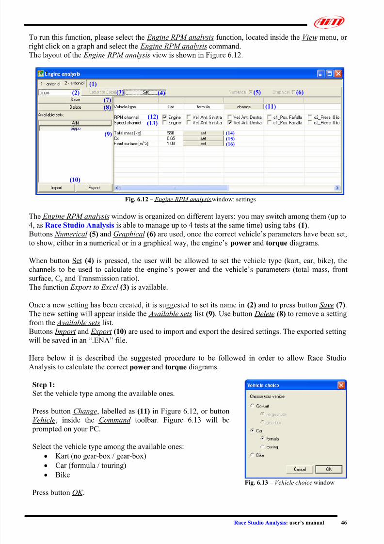
7/27/2019 AIM Manual
http://slidepdf.com/reader/full/aim-manual 46/66
Race Studio Analysis: user’s manual 46
To run this function, please select the Engine RPM analysis function, located inside the View menu, or
right click on a graph and select the Engine RPM analysis command.
The layout of the Engine RPM analysis view is shown in Figure 6.12.
Fig. 6.12 – Engine RPM analysis window: settings
(1)
(3) (5) (6)(2) (4)(7)
(8) (11)
(13)(12)
(14)(15)(16)
(9)
(10)
The Engine RPM analysis window is organized on different layers: you may switch among them (up to
4, as Race Studio Analysis is able to manage up to 4 tests at the same time) using tabs (1).
Buttons Numerical (5) and Graphical (6) are used, once the correct vehicle’s parameters have been set,
to show, either in a numerical or in a graphical way, the engine’s power and torque diagrams.
When button Set (4) is pressed, the user will be allowed to set the vehicle type (kart, car, bike), the
channels to be used to calculate the engine’s power and the vehicle’s parameters (total mass, front
surface, Cx and Transmission ratio).
The function Export to Excel (3) is available.
Once a new setting has been created, it is suggested to set its name in (2) and to press button Save (7).
The new setting will appear inside the Available sets list (9). Use button Delete (8) to remove a setting
from the Available sets list.
Buttons Import and Export (10) are used to import and export the desired settings. The exported setting
will be saved in an “.ENA” file.
Here below it is described the suggested procedure to be followed in order to allow Race Studio
Analysis to calculate the correct power and torque diagrams.
Step 1:Set the vehicle type among the available ones.
Press button Change, labelled as (11) in Figure 6.12, or button
Vehicle, inside the Command toolbar. Figure 6.13 will be
prompted on your PC.
Select the vehicle type among the available ones:
• Kart (no gear-box / gear-box)
• Car (formula / touring)
• Bike
Press button OK .
Fig. 6.13 – Vehicle choice window

7/27/2019 AIM Manual
http://slidepdf.com/reader/full/aim-manual 47/66
Race Studio Analysis: user’s manual 47
Step 2:
Set the vehicle total mass.
Press button Set (14). Figure 6.14 will be prompted on your PC.
Insert the vehicle + driver mass and press button OK .
Do not exceed the maximum / minimum suggested values.
If you set a value greater than the maximum one (or lower than
the minimum one), it will be red highlighted in Figure 6.12.
Fig. 6.14 – Vehicle Mass window
Step 3:
Set the vehicle front surface.
Press button Set (16). Figure 6.14 will be prompted on your PC.
Insert the vehicle’s front surface and press button OK .
Do not exceed the maximum / minimum suggested values.If you set a value greater than the maximum one (or lower than
the minimum one), it will be red highlighted in Figure 6.12.
Fig. 6.15 – Front surface window
Step 4:
Set the vehicle Cx (aerodynamic resistance coefficient).
Press button Set (15). Figure 6.14 will be prompted on your PC.
Insert the Cx value and press button OK .
Do not exceed the maximum / minimum suggested values.If you set a value greater than the maximum one (or lower than
the minimum one), it will be red highlighted in Figure 6.12.
Fig. 6.16 – Vehicle Cx window
Step 5 (no gear-box karts only):
Set the transmission ratio.
Press button Set corresponding to the transmission ratio (not
shown in Figure 6.12). Figure 6.17 will be prompted on your
PC.Insert the pinion and crown teeth number and press button OK .
Do not exceed the maximum / minimum suggested values.
If you set a value greater than the maximum one (or lower than
the minimum one), it will be red highlighted in Figure 6.12.Fig. 6.17 – Transmission ratio window
Step 6:
Set the RPM and Speed channels: place a check besides the desired RPM (12) and Speed (13) channel.
It is reminded that, if your gauge is not able to sample the speed channel (for instance: MyChron 3
Basic), the algorithm will calculate it using the RPM, the transmission ratio and the wheel
circumference.

7/27/2019 AIM Manual
http://slidepdf.com/reader/full/aim-manual 48/66
Race Studio Analysis: user’s manual 48
Once all these parameters have been set, it is suggested to save the new settings:
• Insert the setting name inside (2);
• Press button Save (7).
Now you may press button Set (4) in order to visualize the engine’s power and torque diagrams, as
shown in Figure 6.18.
Fig. 6.18 – Engine RPM analysis window: Graphical compare - Power and Torque diagrams
The torque diagram, green coloured, is shown in the upper part of Figure 6.18.
The power diagram, blue coloured, is shown in the lower part of Figure 6.18. Together with the power
diagram, it is shown (red spots) the experimental values corresponding to the engine’s power.
It is reminded that the user may set the desired unit of measure (CV or HP for power diagram and
kgm or lb*ft for torque diagram) using the File - Preferences function.
If button Numerical (5) is pressed, it will be shown the numerical values corresponding to the power
and torque diagrams, as shown in Figure 6.19.
Fig. 6.19 – Engine RPM analysis window: numerical compare
The RPM, Power and Torque values are organized on three columns (on the left), while on the right itis shown the maximum value for both power and torque, and the corresponding RPM.
The Export to Excel function is enabled: you may export such values, in order to analyse them using
Microsoft Excel ™.
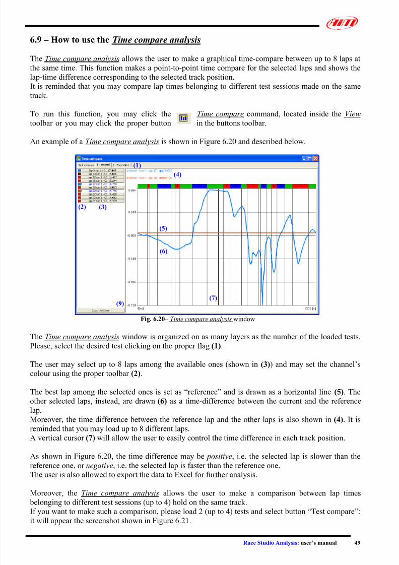
7/27/2019 AIM Manual
http://slidepdf.com/reader/full/aim-manual 49/66
Race Studio Analysis: user’s manual 49
6.9 – How to use the Time compare analysis
The Time compare analysis allows the user to make a graphical time-compare between up to 8 laps at
the same time. This function makes a point-to-point time compare for the selected laps and shows the
lap-time difference corresponding to the selected track position.
It is reminded that you may compare lap times belonging to different test sessions made on the same
track.
To run this function, you may click the Time compare command, located inside the View
toolbar or you may click the proper button in the buttons toolbar.
An example of a Time compare analysis is shown in Figure 6.20 and described below.
Fig. 6.20 – Time compare analysis window
(1)
(4)
(2) (3)
(5)
(6)
(7)(9)
The Time compare analysis window is organized on as many layers as the number of the loaded tests.
Please, select the desired test clicking on the proper flag (1).
The user may select up to 8 laps among the available ones (shown in (3)) and may set the channel’s
colour using the proper toolbar (2).
The best lap among the selected ones is set as “reference” and is drawn as a horizontal line (5). Theother selected laps, instead, are drawn (6) as a time-difference between the current and the reference
lap.
Moreover, the time difference between the reference lap and the other laps is also shown in (4). It is
reminded that you may load up to 8 different laps.
A vertical cursor (7) will allow the user to easily control the time difference in each track position.
As shown in Figure 6.20, the time difference may be positive, i.e. the selected lap is slower than the
reference one, or negative, i.e. the selected lap is faster than the reference one.
The user is also allowed to export the data to Excel for further analysis.
Moreover, the Time compare analysis allows the user to make a comparison between lap times belonging to different test sessions (up to 4) hold on the same track.
If you want to make such a comparison, please load 2 (up to 4) tests and select button “Test compare”:
it will appear the screenshot shown in Figure 6.21.
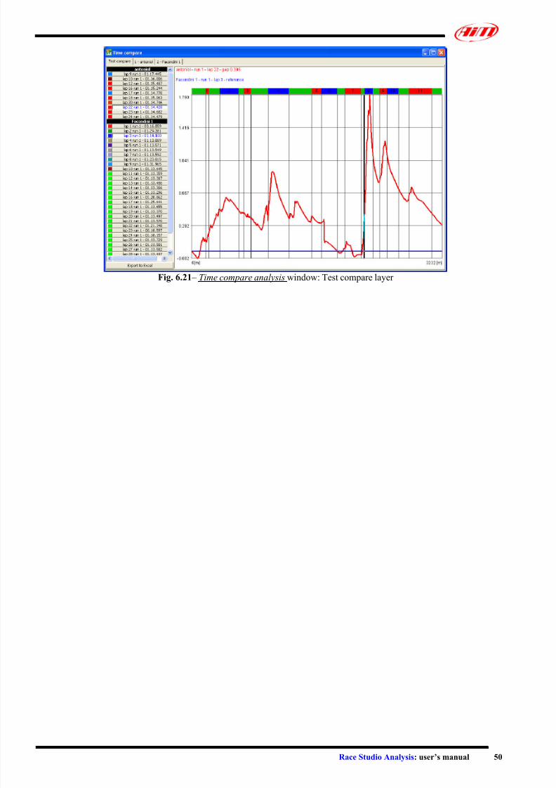
7/27/2019 AIM Manual
http://slidepdf.com/reader/full/aim-manual 50/66
Race Studio Analysis: user’s manual 50
Fig. 6.21 – Time compare analysis window: Test compare layer

7/27/2019 AIM Manual
http://slidepdf.com/reader/full/aim-manual 51/66
Race Studio Analysis: user’s manual 51
Chapter 7 – “How to use the data animation functions”
7.1 – Introduction
The “data animation” functions allow the user to automatically move the cursors of graphs, reports and
maps and to generate a graphical simulation of sampled data.
In fact, it is possible to simulate the driver’s dashboard (RPM, speed, throttle and brake pedals
position, gear and steering angle) and to graphically compare two laps (watching a lap replay).
These functions may be very useful to improve the driver’s performances.
7.2 – How to use the Data animation function
To run this function, you may click the Animation command, located inside the View
toolbar, you may click the proper button in the buttons toolbar or you may use the shortcut
“F12”.
The Animation command allows moving automatically the linked cursors of plots, reports, map,
dashboard and replays.
7.3 – How to use the Lap replay command
The Lap replay command allows seeing a replay and a comparison of two different laps. The laps can
belong to the same test or to two separate tests.
The Lap replay dialog window shows a track drawing (with different colours for each part) and two
coloured cursors (one for each lap) moving on the track (signed (2) in Figure 7.1).
To run this function, you may click the Lap replay command, located inside the View toolbar or youmay use the shortcut “CTRL+F10”.
The layout of the Lap replay window is shown in Figure 7.1.
Fig. 7.1 – Lap replay window
(1) (3) (5)
(6)
(10)(9)
(8)(7)
(2)
(4)
(11) (14)
(12) (15)(13)

7/27/2019 AIM Manual
http://slidepdf.com/reader/full/aim-manual 52/66
Race Studio Analysis: user’s manual 52
Each cursor simulates the position of the vehicle on the track. The cursor for the first lap is painted
cyan (3) while the one for the second lap is painted magenta (4).
The cursors motion may be automatic or manual; when the automatic style is selected the cursors are
linked to the Animation function and to the cursors of the other views (like plots). If the manual style is
chosen four buttons (13) are provided in order to move the cursors on the track.
For each position on the track the difference, in time (14) and in distance (11), between the two laps is
also displayed; the Lap replay window also shows the current distance (15) between the first lap and
the start line.
Pushbutton “start” (12) will allow you to return to the beginning of the current lap and to restart the lap
replay.
If you wish to select a lap, please click with the mouse cursor on the desired lap in (6). The Lap replay
function is able to manage lap compares between different tests: to switch between tests, please select
the desired one in (5).
The Lap replay function is able to show, together with the vehicle’s track position, two sampled
channels for each selected lap. To set the desired channels, please use the menus (7) and (9); the
sampled data belonging to these channels are shown in (8) and (10).
Option/Display Use
Distance (11) Shows the difference in metres or feet between the two laps. The colour of the
next bar-graph depends on the leading lap.
Time (14) Shows the difference in seconds between the two laps. The colour of the next
bar-graph depends on the leading lap.
Position (15) Shows the distance in metres or feet from the start of the leading lap.
Manual run (13) The four buttons of the manual run allow moving the cursors on the track. If the automatic motion is selected these buttons are disabled.
Automatic/Manual To switch from manual replay to automatic replay, please run the Animation
function (shortcut “F12”).
Start (12) Choose this command to position the cursors at the start.
7.4 – How to use the Dashboard function
The “Dashboard” view command allows showing the simulation, in a dashboard like view, of RPM,
speed, brake pedal position, steering wheel angle, throttle pedal position and gear number (if availableor, otherwise, if calculated as a math channel).
The simulation of the dashboard is linked to the cursor motion of plots and to the Animation.
To run this function, you may click the Dashboard command, located inside the View toolbar,
you may use the proper button in the buttons toolbar or you may use the shortcut
“CTRL+F11”.
When the command is run, the Dashboard window is shown as in Figure 7.2.

7/27/2019 AIM Manual
http://slidepdf.com/reader/full/aim-manual 53/66
Race Studio Analysis: user’s manual 53
Fig. 7.2 – Dashboard window
Layout description:
(1) Numerical RPM value.
(2) Analogue RPM value.
(3) The alarm circle becomes red when the RPM value reaches the limiting threshold value.
(4) Numerical speed value.
(5) Analogue speed value.(6) Brake pedal position.
(7) Steering wheel position.
(8) Throttle pedal position.
(9) Engaged gear.
To add/modify a channel to the Dashboard simulator, please right-click on the dashboard area: the
Dashboard setup window is shown in Figure 7.3 and described below.
Fig. 7.3 – Dashboard setup window
(1) (7)(2) (8)
(3)
(9)
(4)
(5) (10)(6) (11)

7/27/2019 AIM Manual
http://slidepdf.com/reader/full/aim-manual 54/66
Race Studio Analysis: user’s manual 54
To add/remove a channel displayed on the Dashboard simulation or to modify the Dashboard settings,
please follow the instructions reported here below.
Option Use
Speed channel Select if the visualisation of the speed is enabled or disabled (1).
If it is enabled, please set the correct speed channel from the channels list
using the menu (2).
RPM channel Select if the visualisation of the RPM is enabled or disabled (3).
If it is enabled, please input the limiting threshold value for the RPM (4).
Brake position Select if the visualisation of the brake pedal position is enabled or disabled
(5).
If it is enabled, please set the correct brake pedal channel from the channels
list using the menu (6).
Steering angle Select if the visualisation of the steering wheel is enabled or disabled (7).
If the display is enabled, please select the steering wheel channel among the
recorded ones (8).
Then select the sign of the channel values (greater or lower than zero) when
the steering wheel is turned to the right (9).
Throttle position Select if the visualisation of the throttle pedal position is enabled or disabled
(10).
If the display is enabled, select the throttle channel among the recorded ones
(11).
Ok Choose this command to exit the dialog window applying the changes.
Cancel Choose this command to exit the dialog window.

7/27/2019 AIM Manual
http://slidepdf.com/reader/full/aim-manual 55/66
Race Studio Analysis: user’s manual 55
Chapter 8 – “How to use the Math channels”
8.1 – Introduction to Math channels
Race Studio Analysis allows analysing two different kinds of measures: Input channels and Math
channels.
The data logger acquires the Input channels (for example speed or oil pressure), while the user defines
the Math channels and the program calculates them on the PC using the Input channels or the Math
channels themselves
Examples of math channels are “gear number”, “Wheel-power”, “Slip factor” etc…
These channels are intended for expert users only.
8.2 – Math channels window’s description
Race Studio Analysis math formula interpreter is a general-purpose, full featured interpreter that
works with the natural math language syntax.
Each formula may include identifiers, constants, functions, symbols and operators:
• The identifiers are the input or the math channels;
• The constants are symbolic constant values user-defined. For example, the acceleration of
gravity ACCGRAV = 9.81 m/s2 is a constant;
• The symbols and the operators allow the user to create a math formula;
• The functions are predefined math formulas: the user has to set the argument of the functions.
To run this function, you may click the Math channels command, located inside the Modify
toolbar, you may use the proper button in the buttons toolbar or you may use the shortcut“ALT+F8”.
The Math channel window is shown in Figure 8.1 and described below.
Fig. 8.1 – Math channels window
(1)
(2) (3) (4)
(14)(13)
(17)(16)
(18)(15)
(8)
(7)
(6) (9)
(5)
(10)
(19)
(20)
(21)
(12)
(11)
7/27/2019 AIM Manual
http://slidepdf.com/reader/full/aim-manual 56/66
Race Studio Analysis: user’s manual 56
In the window’s upped side it is shown 5 checkboxes (1): the “General” one is always enabled, while
the other ones are enabled if the corresponding test has been loaded (in Figure 8.1 it has been loaded
one test only). The selected checkbox will start blinking.
When the “General” box is checked, the predefined math channels are shown in (5). When you click
over a math channel, you can see its properties in the “channel parameters” panel (4), and its
associated math formula in the “Formula” panel (10).
With the buttons “Insert” (3) and Delete (2) you may insert or delete channels; if you need to modify
an existing math channel, you have to select it and change the parameters (4) and/or the math formula.
To change the formula, you may either manually edit the string (10) or use the four panels “Constants”
(13), “Symbols & operators” (14), “Identifiers” (15) and “Functions” (16) to automatically build-up
the formula. If you double click on an item of these four panels, the corresponding item is
automatically copied inside the “formula” panel (10).
If you wish to add to currently loaded test a predefined math channel, please select it from the channel
list (5) and press button “Add” (6): the test name will appear in (9). Then select the currently loaded
test from the checkboxes (1) and click button “Paste” (7). The math channel, now, will appear in thechannel list (5) of the current test.
To delete a math channel from (9), please use button “Empty” (8).
Once the formula has been defined, you should use the button “Test channel” (12) to check if the
formula has been correctly interpreted. You can find the result of this check in the grey line (11) below
the formula string. If there is something wrong you can see the offending item highlighted in the
formula string (10). It is suggested to try to misspell some identifiers or constants to see how the “Test
channel” function works.
The Math channels window also allows the user to set the new channel as a “speed” one (17). If
checkbox (17) is enabled, the user is also allowed to set this channel as “Reference speed” (see paragraph 5.4 “How to modify the reference speed”).
Moreover, the new Math channels graphical interface also allows the user to “Automatically insert the
channel into the DRK file” each time a DRK file is opened. Moreover, if you enable the checkbox
“Overwrite channels with the same name”, each channel labelled as the one you are going to insert will
be overwritten.
The new Math channels window also allows the user to import (19) or export (20) the math channels
set. Moreover, you may load a “Default math channels set” by pressing button Default AIM set (21).
For further information and examples concerning the insertion of a predefined/new math
channel, please refer to chapters 8.3 and 8.4.
8.2.1 – The predefined math channels
Race Studio Analysis provides a list of predefined math channels shown in (5). Each customer may
both use these channels and create his own predefined math channels.
User defined math channels will not be removed or deleted when upgrading the software.
The predefined math channels list is described here below.
Name Description Needed channels Parameters
Wheel Power The available engine power. Reference speed. Vehicle weight.
7/27/2019 AIM Manual
http://slidepdf.com/reader/full/aim-manual 57/66
Race Studio Analysis: user’s manual 57
Slip Factor The ratio between the
reference speed and the
engine rpm.
Reference speed and
engine rpm.
None.
Gear no. Calculates the current gear
number.
Reference speed and
engine RPM.
The maximum and
minimum really used gear
number.
Time For every lap is calculated
the elapsed time from the
start of the lap
None. None.
Calculated speed The maximum, the minimum
or the average between
Speed #1 and Speed #2. This
channel can be selected as
reference speed .
Two speeds input
channels.
The algorithm for the
calculation
Kus A representation of
understeer/oversteer.
Speed, lateral
acceleration and
steering angle.
The wheel base of the
vehicle and the threshold
value for the lateral
acceleration.
DistanceMeters For every lap is calculated
the travelled distance in
meters
Reference speed. None.
DistanceFeet For every lap is calculated
the travelled distance in Feet
Reference speed. None.
8.2.2 – The “Channel parameters” panel
The “Channel parameters” panel (4) allows changing the math channel name, the unit of measure, the
minimum and maximum plotting scale values and the sampling rate.
It is also possible to “filter” the math channel if data are very noisy (for further information on filters,
refer to chapter 4.6.4).
The “Channel parameters” panel also allows the user to define a math channel as a “speed channel”.
For instance, if you have two speed sensors installed on the vehicle, you may create a math channel
called “average speed” with the following equation2
21 Speed Speed +and use this channel as reference
speed (for further information on changing the reference speed, please see chapter 5.4).
8.2.3 – The “Formula” box
In the “Formula” box (10) it is shown the math formula used to calculate the math channel.
This formula is totally modifiable: to change the formula you may either use the “Formula
construction” tools or manually edit the string.
8.2.4 – The “constants” table
The “Constants” table (13) shows a list of predefined constants: these constants load some commonnumbers (such as the acceleration of gravity, the mass of the vehicle, etc…). These values may be used
in the formulas.

7/27/2019 AIM Manual
http://slidepdf.com/reader/full/aim-manual 58/66
Race Studio Analysis: user’s manual 58
Pressing button “New” it is possible to create a new constant: the user has to define its value and the
name. It is suggested to use a name which reminds the function of the constant: for instance, the
constant MI2KM changes the distance’s unit of measure from Miles (MI) to Kilometres (km).
To add a new constant, please press button “New” and define the constant’s value and name. To delete
a constant, please select it from the list and press button “Delete”.
8.2.5 – The “Symbols & operators” table
This panel (14) contains five formula operators (+ - * / ^), the commas (used as function parameters
separator) and the brackets (used to define the precedence of operator and functions).
Please, refer to next table to have a more detailed explanation of “Symbols and Operators”:
Operator Parameters Result
+ (sum) A,B could be
- Integer numbers
- Decimal numbers- Identifiers
- Constants
A+B
- (subtraction) A,B could be
- Integer numbers
- Decimal numbers
- Identifiers
- Constants
A-B
* (product) A,B could be
- Integer numbers
- Decimal numbers
- Identifiers
- Constants
A*B
/ (division) A,B could be
- Integer numbers
- Decimal numbers
- Identifiers
- Constants
A/B
^ (integer power) A could be
- Integer number - Decimal number
- Identifier
- Constant
B must be
- integer number
A^B
Parentheses “()” and comma “,” Parentheses are used to include the argument of a function and to
give the math formula a correct syntactic form.
Commas are used to separate the identifiers inside the functions.
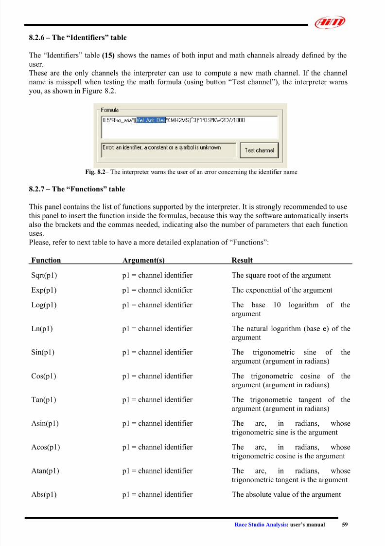
7/27/2019 AIM Manual
http://slidepdf.com/reader/full/aim-manual 59/66
Race Studio Analysis: user’s manual 59
8.2.6 – The “Identifiers” table
The “Identifiers” table (15) shows the names of both input and math channels already defined by the
user.
These are the only channels the interpreter can use to compute a new math channel. If the channel
name is misspell when testing the math formula (using button “Test channel”), the interpreter warns
you, as shown in Figure 8.2.
Fig. 8.2 – The interpreter warns the user of an error concerning the identifier name
8.2.7 – The “Functions” table
This panel contains the list of functions supported by the interpreter. It is strongly recommended to use
this panel to insert the function inside the formulas, because this way the software automatically inserts
also the brackets and the commas needed, indicating also the number of parameters that each function
uses.
Please, refer to next table to have a more detailed explanation of “Functions”:
Function Argument(s) Result
Sqrt(p1) p1 = channel identifier The square root of the argument
Exp(p1) p1 = channel identifier The exponential of the argument
Log(p1) p1 = channel identifier The base 10 logarithm of the
argument
Ln(p1) p1 = channel identifier The natural logarithm (base e) of the
argument
Sin(p1) p1 = channel identifier The trigonometric sine of the
argument (argument in radians)
Cos(p1) p1 = channel identifier The trigonometric cosine of the
argument (argument in radians)
Tan(p1) p1 = channel identifier The trigonometric tangent of the
argument (argument in radians)
Asin(p1) p1 = channel identifier The arc, in radians, whose
trigonometric sine is the argument
Acos(p1) p1 = channel identifier The arc, in radians, whose
trigonometric cosine is the argument
Atan(p1) p1 = channel identifier The arc, in radians, whose
trigonometric tangent is the argument
Abs(p1) p1 = channel identifier The absolute value of the argument
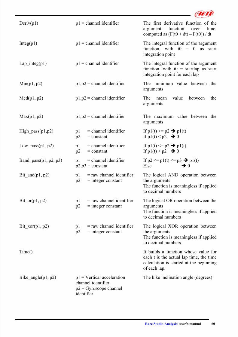
7/27/2019 AIM Manual
http://slidepdf.com/reader/full/aim-manual 60/66
Race Studio Analysis: user’s manual 60
Deriv(p1) p1 = channel identifier The first derivative function of the
argument function over time,
computed as (F(t0 + dt) – F(t0)) / dt
Integ(p1) p1 = channel identifier The integral function of the argument
function, with t0 = 0 as start
integration point
Lap_integ(p1) p1 = channel identifier The integral function of the argument
function, with t0 = startlap as start
integration point for each lap
Min(p1, p2) p1,p2 = channel identifier The minimum value between the
arguments
Med(p1, p2) p1,p2 = channel identifier The mean value between the
arguments
Max(p1, p2) p1,p2 = channel identifier The maximum value between thearguments
High_pass(p1,p2) p1 = channel identifier
p2 = constant
If p1(t) >= p2Î p1(t)
If p1(t) < p2 Î 0
Low_pass(p1, p2) p1 = channel identifier
p2 = constant
If p1(t) <= p2Î p1(t)
If p1(t) > p2 Î 0
Band_pass(p1, p2, p3) p1 = channel identifier
p2,p3 = constant
If p2 <= p1(t) <= p3Î p1(t)
Else Î 0
Bit_and(p1, p2) p1 = raw channel identifier p2 = integer constant The logical AND operation betweenthe arguments
The function is meaningless if applied
to decimal numbers
Bit_or(p1, p2) p1 = raw channel identifier
p2 = integer constant
The logical OR operation between the
arguments
The function is meaningless if applied
to decimal numbers
Bit_xor(p1, p2) p1 = raw channel identifier
p2 = integer constant
The logical XOR operation between
the arguments
The function is meaningless if appliedto decimal numbers
Time() It builds a function whose value for
each t is the actual lap time, the time
calculation is started at the beginning
of each lap.
Bike_angle(p1, p2) p1 = Vertical acceleration
channel identifier
p2 = Gyroscope channel
identifier
The bike inclination angle (degrees)
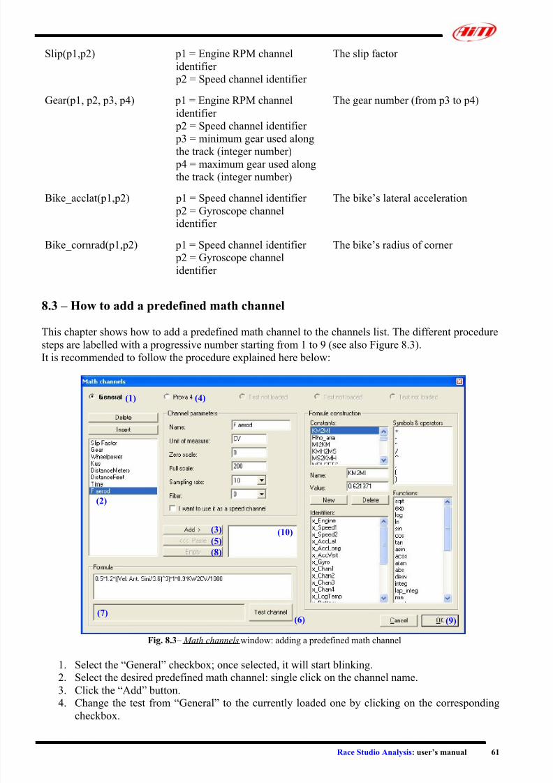
7/27/2019 AIM Manual
http://slidepdf.com/reader/full/aim-manual 61/66
Race Studio Analysis: user’s manual 61
Slip(p1,p2) p1 = Engine RPM channel
identifier
p2 = Speed channel identifier
The slip factor
Gear(p1, p2, p3, p4) p1 = Engine RPM channel
identifier
p2 = Speed channel identifier
p3 = minimum gear used alongthe track (integer number)
p4 = maximum gear used along
the track (integer number)
The gear number (from p3 to p4)
Bike_acclat(p1,p2) p1 = Speed channel identifier
p2 = Gyroscope channel
identifier
The bike’s lateral acceleration
Bike_cornrad(p1,p2) p1 = Speed channel identifier
p2 = Gyroscope channel
identifier
The bike’s radius of corner
8.3 – How to add a predefined math channel
This chapter shows how to add a predefined math channel to the channels list. The different procedure
steps are labelled with a progressive number starting from 1 to 9 (see also Figure 8.3).
It is recommended to follow the procedure explained here below:
Fig. 8.3 – Math channels window: adding a predefined math channel
(4)(1)
(2)
(5)
(8)
(3) (10)
(7)(6) (9)
1. Select the “General” checkbox; once selected, it will start blinking.
2. Select the desired predefined math channel: single click on the channel name.
3. Click the “Add” button.
4. Change the test from “General” to the currently loaded one by clicking on the corresponding
checkbox.

7/27/2019 AIM Manual
http://slidepdf.com/reader/full/aim-manual 62/66
Race Studio Analysis: user’s manual 62
5. Click the “Paste” button: this function copies the math channel from the general math channels
list to the one corresponding to the loaded test.
6. Test the math formula using button “Test channel”. If there in no warning and it appears the
text “OK, the formula has been correctly interpreted”, skip to point 9.
7. If it appears a warning message in (7), you have to fix the problem. The most common problem
concerns misspell constant names or incorrect channel names: this last event is quite common
because the predefined math channels use default channel names (such as “x_Engine”) while
the user may have saved that channel with another name (such as “RPM” or “Engine_RPM”,
etc…). The offending item is blue-highlighted: please, double-click on the correct channel (or
constant) name to replace the incorrect parameter.
8. Click “Empty” to delete the pasted channel from (10).
9. Click button “OK” to apply the changes.
8.4 – How to add a new math channel
This chapter shows how to add a new channel to the math channel list.
For instance, the example reported here below shows how to add the math channel “average speed” to
the currently loaded test channel list (in this example, it is supposed that two speed signals have been
sampled).
1. Select the checkbox corresponding to the loaded test.
2. Click the “Insert” button.
3. Input the channel name in the corresponding box (located inside the “Channel parameters”
panel): for instance, digit “avg_speed”.
4. Input the channel’s unit of measure: km/h, m/s, MPH, etc…
5. Set the plotting scale limits (i.e. the zero/full scale).
6. Do not modify the “Sampling frequency” menu: the correct sampling frequency is fixed by the
program.
7.
As this new math channel is a speed one, place a check besides the “I want to use it as a speedchannel” box. This event will allow you choosing this new channel as “Reference speed”.
8. Now you are able to insert the math formula inside the “Formula” panel. It is strongly
recommended to use the “Formula construction” panel to insert the formula, because this way
the software automatically inserts the brackets and the commas needed.
9. Now select from the “Functions” list the “med” one and double click on it.
10. It is reminded that, as previously explained in chapter 8.2.7, the function “med” needs 2
identifiers, which are the first and the second speed channel
11. Once double-clicked on the function, it will appear in the “Formula” panel in the following
way: med(,)
12. Now click with the mouse in the space between the open-bracket “(” and the comma “,” in
order to set the first identifier and, then, select the correct first speed channel from the“Identifiers” list by double-clicking on it.
13. Now click with the mouse in the space between the comma “,” and the close-bracket “)” in
order to set the second identifier and, then, select the correct second speed channel from the
“Identifiers” list by double-clicking on it.
14. Now you may test the new math channel by pressing the “Test channel” function.
15. If the parameters/identifiers have been correctly set, it will appear the text “OK, the formula
has been correctly interpreted”. Click “OK” to save the new channel inside the currently loaded
test’s channel list.

7/27/2019 AIM Manual
http://slidepdf.com/reader/full/aim-manual 63/66
Race Studio Analysis: user’s manual 63
Chapter 9 – Utility functions
9.1 – How to change the messages language
Race Studio Analysis has been designed to manage multi-languages using a database.
To change the text/messages language, please click the Language command on the commands toolbar.
The Language selection window is shown in Figure 9.1 and described below:
Fig. 9.1 – Language selection window
To change the software language, select the desired one and then click the “OK” button; otherwise, if
you wish to exit without saving, please click button “Cancel”.
9.2 – How to print a graph
If you wish to plot a graph, you may use the Print function, located inside the File toolbar, you
may click the proper button in the buttons toolbar, you may select the Print option by right-
clicking on the graph area or you may use the shortcut “SHIFT+F12”.
Race Studio Analysis also allows the user to have a Print preview of the current graph. To run this
function, please select the Print Preview command inside the File toolbar or use the shortcut
“SHIFT+F11”.
When you are running the Print preview function, you may both zoom in/out the graph and print it. To
exit this function, please press button “Close” or the red cross in the right upper corner of the window.
9.3 – How to modify the unit of measures/wheel number
If you wish to modify the software’s general setup (i.e. the wheel number and the units of measure),
please run the Preferences function by clicking the corresponding command in the File toolbar or
using the shortcut “SHIFT+F6”.
The Preferences window is shown in Figure 9.2 and described below:
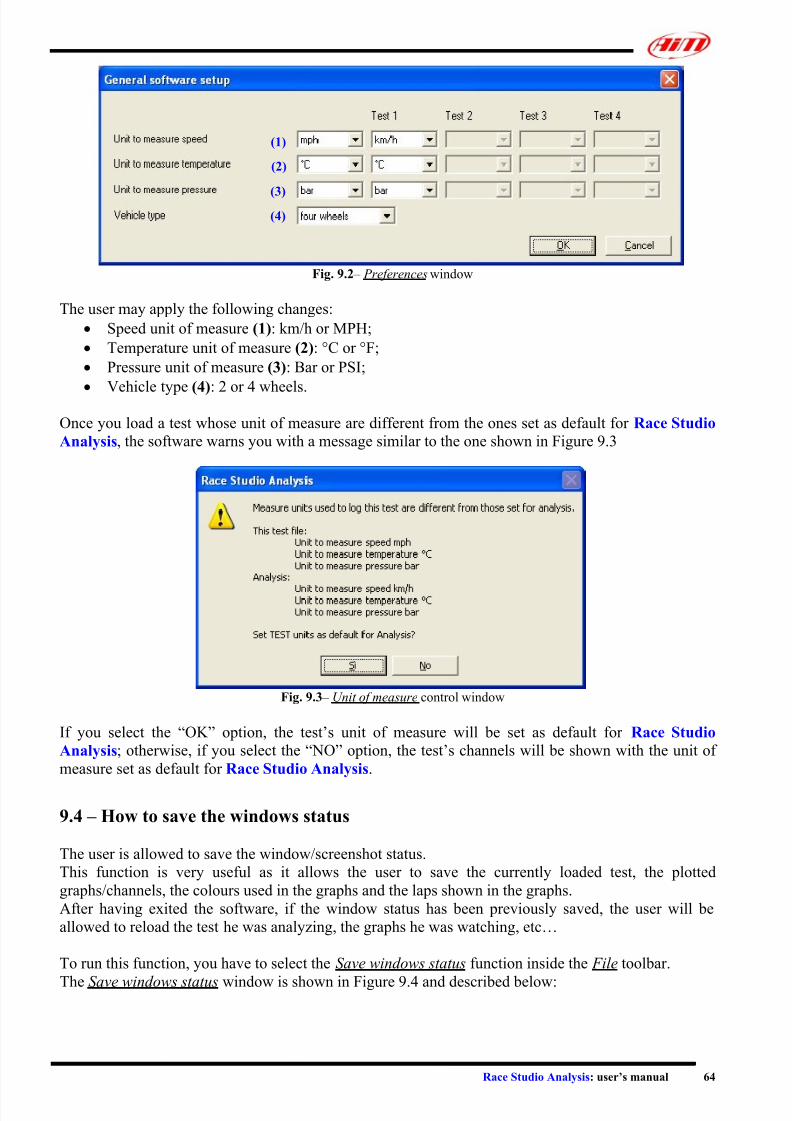
7/27/2019 AIM Manual
http://slidepdf.com/reader/full/aim-manual 64/66
Race Studio Analysis: user’s manual 64
Fig. 9.2 – Preferences window
(1)
(2)
(3)
(4)
The user may apply the following changes:
• Speed unit of measure (1): km/h or MPH;
• Temperature unit of measure (2): °C or °F;
• Pressure unit of measure (3): Bar or PSI;
• Vehicle type (4): 2 or 4 wheels.
Once you load a test whose unit of measure are different from the ones set as default for Race Studio
Analysis, the software warns you with a message similar to the one shown in Figure 9.3
Fig. 9.3 – Unit of measure control window
If you select the “OK” option, the test’s unit of measure will be set as default for Race Studio
Analysis; otherwise, if you select the “NO” option, the test’s channels will be shown with the unit of
measure set as default for Race Studio Analysis.
9.4 – How to save the windows status
The user is allowed to save the window/screenshot status.
This function is very useful as it allows the user to save the currently loaded test, the plotted
graphs/channels, the colours used in the graphs and the laps shown in the graphs.
After having exited the software, if the window status has been previously saved, the user will be
allowed to reload the test he was analyzing, the graphs he was watching, etc…
To run this function, you have to select the Save windows status function inside the File toolbar.
The Save windows status window is shown in Figure 9.4 and described below:
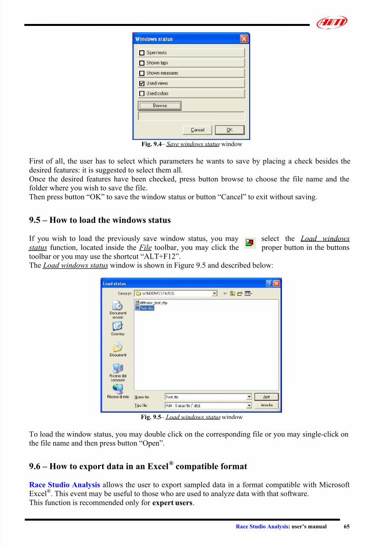
7/27/2019 AIM Manual
http://slidepdf.com/reader/full/aim-manual 65/66
Race Studio Analysis: user’s manual 65
Fig. 9.4 – Save windows status window
First of all, the user has to select which parameters he wants to save by placing a check besides the
desired features: it is suggested to select them all.
Once the desired features have been checked, press button browse to choose the file name and the
folder where you wish to save the file.
Then press button “OK” to save the window status or button “Cancel” to exit without saving.
9.5 – How to load the windows status
If you wish to load the previously save window status, you may select the Load windows
status function, located inside the File toolbar, you may click the proper button in the buttons
toolbar or you may use the shortcut “ALT+F12”.
The Load windows status window is shown in Figure 9.5 and described below:
Fig. 9.5 – Load windows status window
To load the window status, you may double click on the corresponding file or you may single-click on
the file name and then press button “Open”.
9.6 – How to export data in an Excel®
compatible format
Race Studio Analysis allows the user to export sampled data in a format compatible with Microsoft
Excel®. This event may be useful to those who are used to analyze data with that software.
This function is recommended only for expert users.

7/27/2019 AIM Manual
http://slidepdf.com/reader/full/aim-manual 66/66
To run this function, please select the Excel compatible format conversion option inside the File
toolbar. The “Conversion to Excel” window is shown in Figure 9.6.
Fig. 9.6 – Conversion to Excel ® window
(1)
(2) (3)
(4) (5)
(8)
(6) (7)
To export the sampled data to Excel® follow these instructions:
• Select the Channels you wish to export from the channel list (4) by single-clicking on the
channel name. The selected channel becomes blue-highlighted. To select/unselect all channels,
use button (6).
• Select the laps you wish to export from the lap list (5); use button (7) to select/unselect all laps.
• Once the desired channels/laps have been selected, click button “Browse” (1) to set the folder and the file name.
• The channel name and the saving path are shown in (2).
• The user may also set if he wishes to export the channels/laps vs. Distance, vs. Time or vs. both
by placing a check in (8).
• Once all the previously operations have been completed, you may click the “Save” button (3).
9.7 – How to load the user’s manual
If you wish to load the user’s manual when working under Race Studio Analysis, you may
select the Manual command from the ? toolbar, you may click the proper button locatedinside the buttons toolbar or you may use the shortcut “F1”.
9.8 – How to run the AIM electronic documentation library
If you installed Race Studio 2 (version 2.13.13 or later) from a CD-ROM (this feature is not available