AIMMS - unibo.itgabbri/MaterialeCorsi/CP-L3.pdf · Solving CSPs Search algorithm. – Usually backtracking search performing a depth-first traversal of a search tree. Local consistency

AIMMS

  Modeling language with an interface to CP and MIP solvers (http://www.aimms.com/cp)

  Student license   GUI support available only in the Windows version

–  Create a virtual machine with Windows OS in your computer

–  Virtual Box (https://www.virtualbox.org/)   Extensive documentation

–  One-hour tutorial (general introduction) –  Chapter 21 – “Constraint Programming” of Language

Reference

PART II: Local Consistency & Constraint Propagation

Solving CSPs

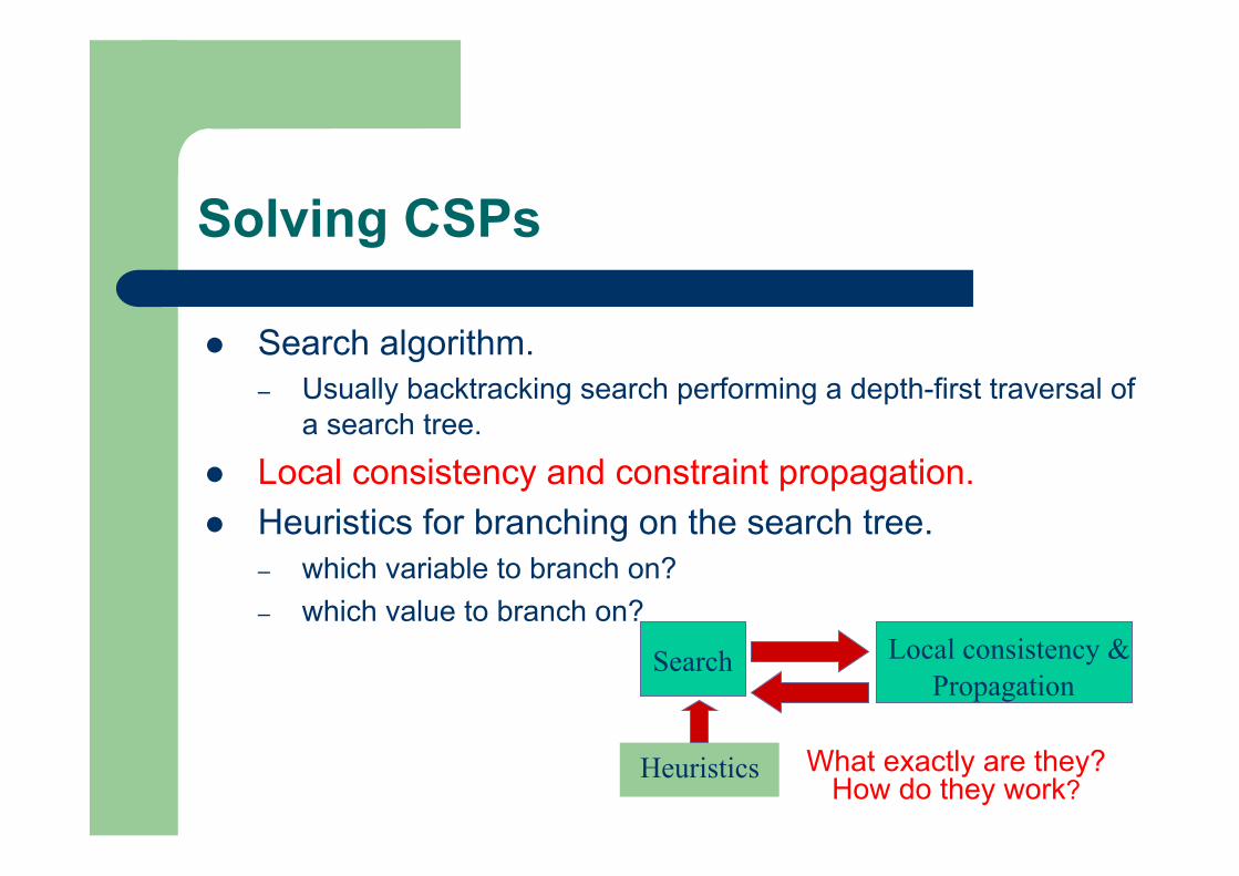
  Search algorithm. –  Usually backtracking search performing a depth-first traversal of

a search tree.

  Local consistency and constraint propagation.   Heuristics for branching on the search tree.

–  which variable to branch on? –  which value to branch on?

Search Local consistency & Propagation

Heuristics

Solving CSPs

  Search algorithm. –  Usually backtracking search performing a depth-first traversal of

a search tree.

  Local consistency and constraint propagation.   Heuristics for branching on the search tree.

–  which variable to branch on? –  which value to branch on?

Search Local consistency & Propagation

Heuristics What exactly are they? How do they work?

Outline

  Local Consistency –  Arc Consistency (AC) –  Generalized Arc Consistency (GAC) –  Bounds Consistency (BC) –  Higher Levels of Consistency

  Constraint Propagation –  Propagation Algorithms

  Specialized Propagation Algorithms –  Global Constraints

  Generalized Propagation Algorithms –  AC algorithms

Local Consistency

  Backtrack tree search aims to extend a partial assignment of variables to a complete and consistent one.

  Some inconsistent partial assignments obviously cannot be completed.

  Local consistency is a form of inference which detects inconsistent partial assignments.

–  Consequently, the backtrack search commits into less inconsistent assignments.

  Local, because we examine individual constraints. –  Global consistency is NP-hard!

Local Consistency: An example

  D(X1) = {1,2}, D(X2) = {3,4}, C1: X1 = X2, C2: X1 + X2 ≥ 1   X1 = 1   X1 = 2   X2 = 3   X2 = 4

–  No need to check the other constraint. –  Unsatisfiability of the CSP can be inferred without having to

search!

all inconsistent partial assignments wrt the constraint C1

Several Local Consistencies

  Most popular local consistencies are domain based: –  Arc Consistency (AC); –  Generalised Arc Consistency (GAC); –  Bounds Consistency (BC).

  They detect inconsistent partial assignments of the form Xi = j, hence: –  j can be removed from D(Xi) via propagation; –  propagation can be implemented easily.

Arc Consistency (AC)

  Defined for binary constraints.   A binary constraint C is a relation on two variables Xi

and Xj, giving the set of allowed combinations of values (i.e. tuples):

–  C ⊆ D(Xi) x D(Xj) –  E.g., D(X1) = {0,1}, D(X2) = {1,2}, C: X1 < X2 C(X1,X2) = {(0,1), (0,2), (1,2)}


  Defined for binary constraints.   A binary constraint C is a relation on two variables Xi

and Xj, giving the set of allowed combinations of values (i.e. tuples):

–  C ⊆ D(Xi) x D(Xj) –  E.g., D(X1) = {0,1}, D(X2) = {1,2}, C: X1 < X2 C(X1,X2) = {(0,1), (0,2), (1,2)}

Each tuple (d1,d2) is called a support for C


  C is AC iff: –  forall v ∈ D(Xi), exists w ∈ D(Xj) s.t. (v,w) ∈ C.

  v ∈ D(Xi) is said to have/belong to a support wrt the constraint C. –  forall w ∈ D(Xj), exists v ∈ D(Xi) s.t. (v,w) ∈ C.

  w ∈ D(Xj) is said to have/belong to a support wrt the constraint C.

  A CSP is AC iff all its binary constraints are AC.

AC: An example

  D(X1) = {1,2,3}, D(X2) = {2,3,4}, C: X1 = X2   AC(C)?

–  1 ∈ D(X1) does not have a support. –  2 ∈ D(X1) has 2 ∈ D(X2) as support. –  3 ∈ D(X1) has 3 ∈ D(X2) as support. –  2 ∈ D(X2) has 2 ∈ D(X1) as support. –  3 ∈ D(X2) has 3 ∈ D(X1) as support. –  4 ∈ D(X2) does not have a support.

  X1 = 1 and X2 = 4 are inconsistent partial assignments.   1 ∈ D(X1) and 4 ∈ D(X2) must be removed to achieve AC.   D(X1) = {2,3}, D(X2) = {2,3}, C: X1 = X2

–  AC(C)

Propagation!

Generalised Arc Consistency

  Generalisation of AC to k-ary constraints.   A constraint C is a relation on k variables X1,…, Xk:

–  C ⊆ D(X1) x … x D(Xk) –  E.g., D(X1) = {0,1}, D(X2) = {1,2}, D(X2) = {2,3} C: X1 + X2 = X3

C(X1,X2,X3) = {(0,2,2), (1,1,2), (1,2,3)}   A support is a tuple (d1,…,dk) ∈ C where di ∈ D(Xi).

Generalised Arc Consistency

  C is GAC iff: –  forall Xi in {X1,…, Xk}, forall v ∈ D(Xi), v belongs to a support.

  AC is a special case of GAC.   A CSP is GAC iff all its constraints are GAC.

GAC: An example

  D(X1) = {1,2,3}, D(X2) = {1,2}, D(X3) = {1,2} C: alldifferent([X1, X2, X3])

  GAC(C)? –  X1 = 1 and X1 = 2 are not supported!

  D(X1) = {3}, D(X2) = {1,2}, D(X3) = {1,2} C: alldifferent([X1, X2, X3])

–  GAC(C)

Bounds Consistency (BC)

  Defined for totally ordered (e.g. integer) domains.   Relaxes the domain of Xi from D(Xi) to [min(Xi)..max(Xi)].

–  E.g., D(Xi) = {1,3,5} [1..5]


  A constraint C is a relation on k variables X1,…, Xk: –  C ⊆ D(X1) x … x D(Xk)

  A bound support is a tuple (d1,…,dk) ∈ C where di ∈ [min(Xi)..max(Xi)].

  C is BC iff: –  forall Xi in {X1,…, Xk}, min(Xi) and max(Xi) belong to a

bound support.


  Disadvantage –  BC might not detect all GAC inconsistencies in general.

  Advantages –  Might be easier to look for a support in a range than in a domain. –  Achieving BC is often cheaper than achieving GAC. –  Achieving BC is enough to achieve GAC for monotonic

constraints.

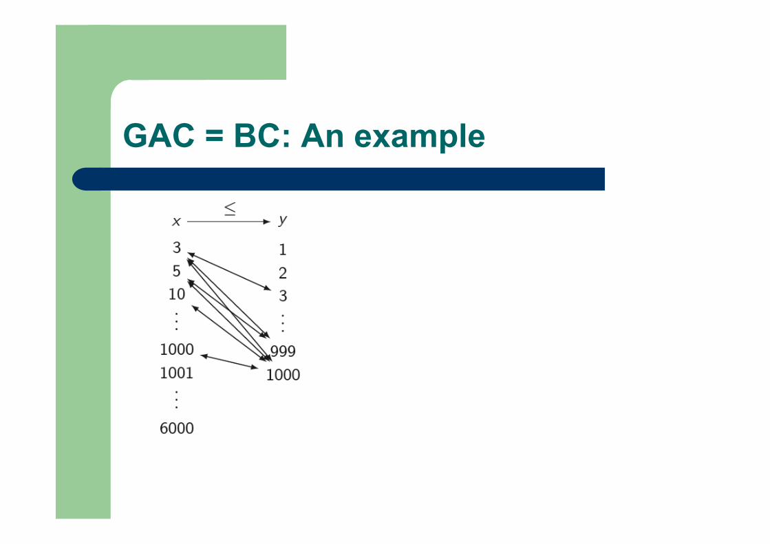
GAC = BC: An example

GAC = BC: An example

  If (v,w) is a support of X ≤ Y, then: –  for all u ∈ D(Y) s.t. u ≥ w:

  (v,u) is also a support; –  for all u ∈ D(X) s.t. u ≤ v:

  (u,w) is also a support.

  All values of D(X) smaller than or equal to max(Y) are GAC.

  All values of D(Y) greater than or equal to min(X) are GAC.

  Enough to adjust max(X) and min(Y).

GAC > BC: An example

  D(X1) = D(X2) = {1,2}, D(X3) = D(X4) = {2,3,5,6}, D(X5) = {5}, D(X6) = {3,4,5,6,7}

C: alldifferent([X1, X2 , X3 , X4 , X5 , X6 ])

  BC(C): 2 ∈ D(X3) and 2 ∈ D(X4) have no support.

Original BC

GAC > BC: An example

  D(X1) = D(X2) = {1,2}, D(X3) = D(X4) = {2,3,5,6}, D(X5) = {5}, D(X6) = {3,4,5,6,7}

C: alldifferent([X1, X2 , X3 , X4 , X5 , X6 ])

  GAC(C): {2,5} ∈ D(X3) , {2,5} ∈ D(X4), {3,5,6} ∈ D(X6) have no support.

Original BC GAC

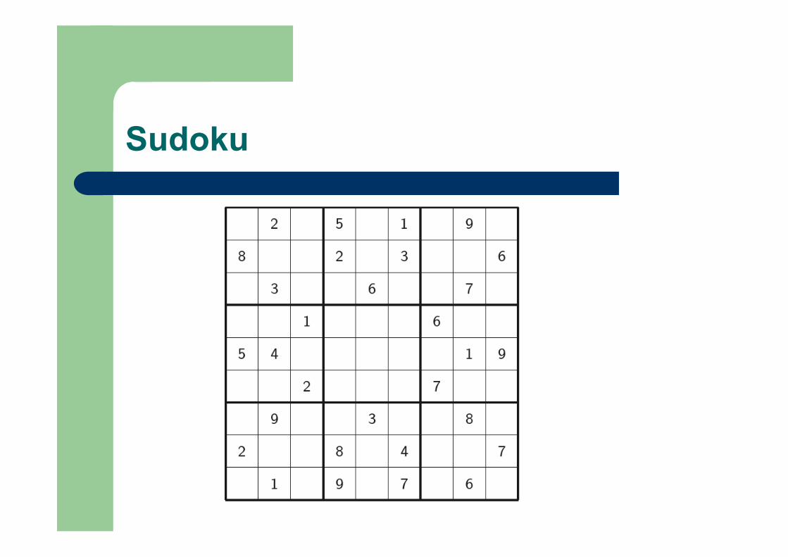
Sudoku

Sudoku

Sudoku with AC(≠)

Sudoku with BC(alldifferent)

Sudoku with GAC(alldifferent)

Higher Levels of Consistencies

  Path consistency, k-consistencies, (i,j) consistencies, …   Not much used in practice:

–  detect inconsistent partial assignments with more than one <variable,value> pair.

–  cannot be enforced by removing single values from domains.

  Domain based consistencies stronger than (G)AC. –  Singleton consistencies, triangle-based consistencies, … –  Becoming popular.

  Shaving in scheduling.

Outline

  Local Consistency –  Arc Consistency (AC) –  Generalised Arc Consistency (GAC) –  Bounds Consistency (BC) –  Higher Levels of Consistency

  Constraint Propagation –  Constraint Propagation Algorithms

  Specialised Propagation Algorithms –  Global Constraints

  Generalized Propagation Algorithms –  AC Algorithms

Constraint Propagation

  Can appear under different names: –  constraint relaxation; –  filtering algorithm; –  local consistency enforcing, …

  Similar concepts in other fields. –  E.g., unit propagation in SAT.

  Local consistencies define properties that a CSP must satisfy after constraint propagation:

–  the operational behavior is completely left open; –  the only requirement is to achieve the required property on the

CSP.

Constraint Propagation: A simple example

Input CSP:D(X1) = {1,2}, D(X2) = {1,2} , C: X1 < X2

Output CSP:D(X1) = {1}, D(X2) = {2} , C: X1 < X2

A constraint propagation algorithm for enforcing AC

We can write different

algorithms with different

complexities to achieve the same effect.

Constraint Propagation Algorithms

  A constraint propagation algorithm propagates a constraint C. –  It removes the inconsistent values from the domains of

the variables of C. –  It makes C locally consistent. –  The level of consistency depends on C:

  GAC might be NP-complete, BC might not be possible, …

Constraint Propagation Algorithms

  When solving a CSP with multiple constraints: –  propagation algorithms interact; –  a propagation algorithm can wake up an already

propagated constraint to be propagated again! –  in the end, propagation reaches a fixed-point and all

constraints reach a level of consistency; –  the whole process is referred as constraint

propagation.

Constraint Propagation: An example

  D(X1) = D(X2) = D(X3)= {1,2,3} C1: alldifferent([X1, X2 , X3 ]) C2: X2 < 3 C3: X3 < 3   Let’s assume:

–  the order of propagation is C1, C2, C3; –  each algorithm maintains (G)AC.

  Propagation of C1: –  nothing happens, C1 is GAC.

  Propagation of C2: –  3 is removed from D(X2), C2 is now AC.

  Propagation of C3: –  3 is removed from D(X3), C3 is now AC.

  C1 is not GAC anymore, because the supports of {1,2} ∈ D(X1) in D(X2) and D(X3) are removed by the propagation of C2 and C3.

  Re-propagation of C1: –  1 and 2 are removed from D(X1), C1 is now AC.

Properties of Constraint Propagation Algorithms

  It is not enough to remove inconsistent values from domains once.

  A constraint propagation algorithm must wake up again when necessary, otherwise may not achieve the desired local consistency property.

  Events that trigger a constraint propagation: –  when the domain of a variable changes; –  when a variable is assigned a value; –  when the minimum or the maximum values of a domain changes.

Outline




  Decompositions   Ad-hoc algorithms


Specialized Propagation Algorithms

  A constraint propagation algorithm can be general or specialized:

–  general, if it is applicable to any constraint; –  specialized, if it is specific to a constraint.

  Specialized algorithms –  Disadvantages

  Limited use.   Not always easy to develop one.

–  Advantages   Exploits the constraint semantics.   Potentially much more efficient than a general algorithm.

  Worth developing for recurring constraints.

Specialized Propagation Algorithms

  C: X1 ≤ X2

  Observation –  A support of min(X2) supports all the values in D(X2). –  A support of max(X1) supports all the values in D(X1).

  Propagation algorithm –  Filter D(X1) s.t. max(X1) ≤ max(X2). –  Filter D(X2) s.t. min(X1) ≤ min(X2).

  The result is GAC (and thus BC).

Example

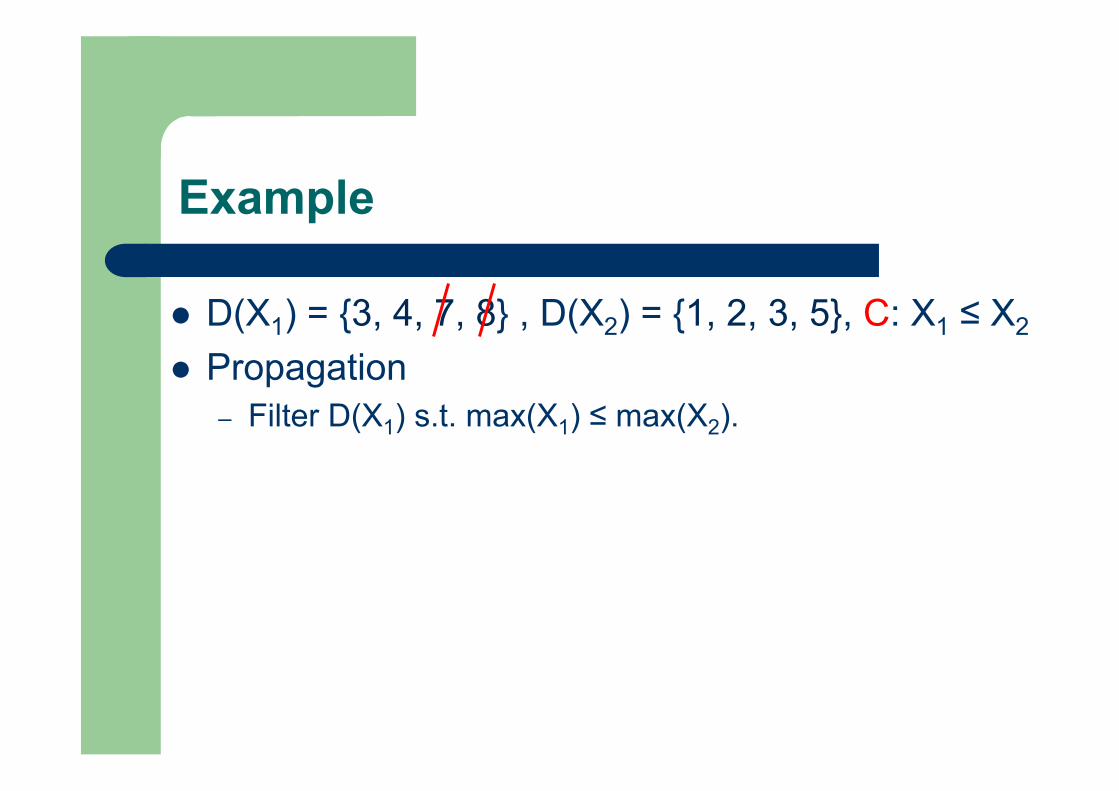
  D(X1) = {3, 4, 7, 8} , D(X2) = {1, 2, 3, 5}, C: X1 ≤ X2

Example

  D(X1) = {3, 4, 7, 8} , D(X2) = {1, 2, 3, 5}, C: X1 ≤ X2

  Propagation –  Filter D(X1) s.t. max(X1) ≤ max(X2).

Example

  D(X1) = {3, 4, 7, 8} , D(X2) = {1, 2, 3, 5}, C: X1 ≤ X2

  Propagation –  Filter D(X1) s.t. max(X1) ≤ max(X2).

Example

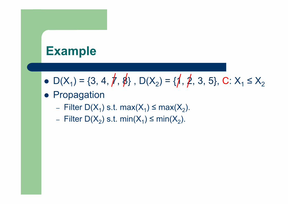
  D(X1) = {3, 4, 7, 8} , D(X2) = {1, 2, 3, 5}, C: X1 ≤ X2

  Propagation –  Filter D(X1) s.t. max(X1) ≤ max(X2). –  Filter D(X2) s.t. min(X1) ≤ min(X2).

Example

  D(X1) = {3, 4, 7, 8} , D(X2) = {1, 2, 3, 5}, C: X1 ≤ X2

  Propagation –  Filter D(X1) s.t. max(X1) ≤ max(X2). –  Filter D(X2) s.t. min(X1) ≤ min(X2).

Global Constraints

  Many real-life constraints are complex and not binary. –  Specialised algorithms are often developed for such constraints!

  A complex and n-ary constraint which encapsulates a specialised propagation algorithm is called a global constraint.

Examples of Global Constraints

  Alldifferent constraint

–  alldifferent([X1, X2, …, Xn]) holds iff Xi ≠ Xj for i < j ∈ {1,…,n}

–  Useful in a variety of context:   timetabling (e.g. exams with common students must occur at

different times)   tournament scheduling (e.g. a team can play at most once in a

week)   configuration (e.g. a particular product cannot have repeating

components)   …

Beyond Alldifferent

  NValue constraint –  One generalization of alldifferent. –  nvalue([X1, X2, …, Xn], N) holds iff

N = |{Xi | 1 ≤ i ≤ n }| –  nvalue([1, 2, 2, 1, 3], 3). –  alldifferent when N = n. –  Useful when values represent resources and we want

to limit the usage of resources. E.g.,   minimize the total number of resources used;   the total number of resources used must be between a

specific interval;   …

Beyond Alldifferent

  Global cardinality constraint –  Another generalisation of alldifferent. –  gcc([X1, X2, …, Xn], [v1, …, vm], [O1, …, Om]) iff

forall j ∈ {1,…, m} Oj = |{Xi | Xi = vj, 1 ≤ i ≤ n }| –  gcc([1, 1, 3, 2, 3], [1, 2, 3, 4], [2, 1, 2, 0]) –  Useful again when values represent resources. –  We can now limit the usage of each resource

individually. E.g.,   resource 1 can be used at most three times;   resource 2 can be used min 2 max 5 times;   …

Symmetry Breaking Constraints

  Consider the following scenario. –  [X1, X2, …, Xn] and [Y1, Y2, …, Yn] represent the 2 day event

assignments of a conference. –  Each day has n slots and the days are indistinguishable. –  Need to avoid symmetric assignments.

  Global constraints developed for this purpose are called symmetry breaking constraints.

  Lexicographic ordering constraint –  lex([X1, X2, …, Xn], [Y1, Y2, …, Yn]) holds iff: X1 < Y1 OR (X1 = Y1 AND X2 < Y2) OR … (X1 = Y1 AND X2 = Y2 AND …. AND Xn ≤ Yn) –  lex ([1, 2, 4],[1, 3, 3])

Sequencing Constraints

  We might want a sequence of variables obey certain patterns.

  Global constraints developed for this purpose are called sequencing constraints.


  Sequence constraint –  Constrains the number of values taken from a given

set in any sequence of k variables. –  sequence(l, u, k, [X1, X2, …, Xn], v) iff

among([Xi, Xi+1, …, Xi+k-1], v, l, u) for 1 ≤ i ≤ n-k+1 –  among([X1, X2, …, Xn], v, l, u) iff

l ≤ |{i | Xi ∈ v, 1 ≤ i ≤ n }| ≤ u –  E.g.,

  every employee has 2 days off in any 7 day of period;   at most 1 in 3 cars along the production line can have a

sun-roof fitted.

  Sometimes patterns can be best described by grammars or automata that accept some language.

  Regular constraint –  regular([X1, X2, …, Xn], A) holds iff <X1, X2, …, Xn> forms a

string accepted by the DFA A (which accepts a regular language).

–  regular([a, a, b], A), regular([b], A), regular([b, c, c, c, c, c], A) with A:

  Many global constraints are instances of regular. E.g., among, lex, strech, …


a b c

Scheduling Constraints

  We might want to schedule tasks with respective release times, duration, and deadlines, using limited resources in a time D.

  Global constraints developed for this purpose are called scheduling constraints.

Scheduling Constraints

  Cumulative constraint –  Useful for scheduling non-preemptive tasks who share a single

resource with limited capacity. –  Given tasks t1,.., tn, with each ti associated with 3 variables Si,

Di, and Ci, and a resource of capacity C: cumulative([S1, S2, …, Sn], [D1, D2, …, Dn], [C1, C2, …, Cn], C)

iff forall u in D

Ci!C

i|Si!u<Si+Di"

Scheduling Example

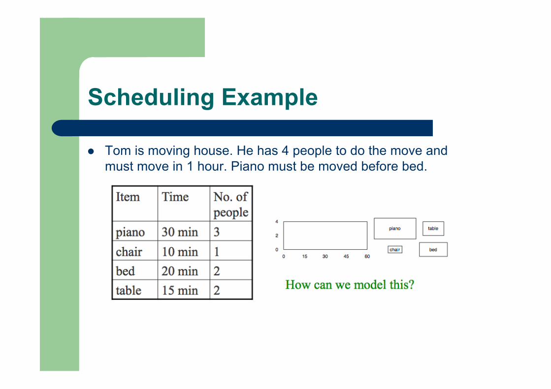
  Tom is moving house. He has 4 people to do the move and must move in 1 hour. Piano must be moved before bed.

Scheduling Example

  Tom is moving house. He has 4 people to do the move and must move in 1 hour. Piano must be moved before bed.

  D(P)=D(C)=D(B)=D(T)=[0..60], P + 30 ≤ B, P + 30 ≤ 60, C + 10 ≤ 60, B + 20 ≤ 60, T + 15 ≤ 60, cumulative([P,C,B,T], [30,10,20,15],[3,1,2,2],4)

Scheduling Example

  6 tasks [a,b,c,d,e,f,g] to place in an 5x20 box with the durations [2,6,2,2,5,6] requiring [1,2,4,2,2,2] units of resource with precedences as in the figure.

  Model –  D(Sa)=D(Sb)=D(Sc)=D(Sd)=D(Se), D(Sf) = [0..20] –  Sa + 2 ≤ Sb, Sb + 6 ≤ Sc, Sd + 2 ≤ Se –  Sa + 2 ≤ 20, Sb + 6 ≤ 20, Sc + 2 ≤ 20, Sd + 2 ≤ 20, Se + 5 ≤ 20, Sf + 6 ≤ 20 –  cumulative([Sa,Sb,Sc,Sd, Se, Sf], [2,6,2,2,5,6],[1,2,4,2,2,2],5)

Specialised Algorithms for Global Constraints

  How do we develop specialized algorithms for global constraints?

  Two main approaches: –  constraint decomposition; –  ad-hoc algorithm.

Constraint Decomposition

  A global constraint is decomposed into smaller and simpler constraints each which has a known propagation algorithm.

  Propagating each of the constraints gives a propagation algorithm for the original global constraint. –  A very effective and efficient method for some global

constraints.

Decomposition of Among

  Among constraint -  among([X1, X2, …, Xn], [d1, d2, …, dm], N) iff

N = |{i | Xi ∈ {d1, d2, …, dm}, 1 ≤ i ≤ n }|

Decomposition of Among

  Among constraint -  among([X1, X2, …, Xn], [d1, d2, …, dm], N) iff

N = |{i | Xi ∈ {d1, d2, …, dm}, 1 ≤ i ≤ n }|   Decomposition –  Bi with D(Bi) = {0, 1} for 1 ≤ i ≤ n –  Ci: Bi = 1 ↔ Xi ∈ {d1, d2, …, dm} for 1 ≤ i ≤ n – 

  AC(Ci) for 1 ≤ i ≤ n and BC( ) ensures GAC on among.

!

Bi= N

i"

!

Bi= N

i"

Decomposition of Lex

  C: lex([X1, X2, …, Xn], [Y1, Y2, …, Yn])   Decomposition

-  Bi with D(Bi) = {0, 1} for 1 ≤ i ≤ n+1 to indicate the vectors have been ordered by position i-1

-  B1= 0 -  Ci: (Bi = Bi+1 = 0 AND Xi = Yi ) OR (Bi = 0 AND Bi+1 = 1 AND Xi < Yi )

OR (Bi = Bi+1 = 1) for 1 ≤ i ≤ n

  GAC(Ci) ensures GAC on C.

Decomposition of Regular

  C: regular([X1, X2, …, Xn], A)   Decomposition

–  Qi for 1 ≤ i ≤ n+1 to indicate the states of the DFA. –  Q1= starting state. –  Qn+1= accepting state. –  Ci (Xi,Qi ,Qi+1) for 1 ≤ i ≤ n. –  Ci (Xi,Qi Qi+1) iff DFA goes from Qi to Qi+1 on symbol

Xi.   GAC(Ci) ensures GAC on C.

Constraint Decompositions

  May not always provide an effective propagation.   Often GAC on the original constraint is stronger than

(G)AC on the constraints in the decomposition.   E.g., C: alldifferent([X1, X2, …, Xn])   Decomposition

–  Cij: Xi ≠ Xj for i < j ∈ {1,…,n} –  AC on the decomposition is weaker than GAC on alldifferent. –  E.g., D(X1) = D(X2) = D(X3) = {1,2}, C: alldifferent([X1, X2, X3]) –  C12, C13, C23 are all AC, but C is not GAC.


  C: lex([X1, X2, …, Xn], [Y1, Y2, …, Yn])   OR decomposition

-  X1 < Y1 OR (X1 = Y1 AND X2 < Y2) OR … (X1 = Y1 AND X2 = Y2 AND …. AND Xn ≤ Yn) -  AC on the decomposition is weaker than GAC on C. -  E.g., D(X1) = {0,1,2} , D(X2) = {0,1}, D(Y1) = {0,1} , D(Y2) = {0,1}

C: Lex([X1, X2], [Y1, Y2]) -  C is not GAC but the decomposition does not prune anything.


  AND decomposition -  X1 ≤ Y1 AND (X1 = Y1 → X2 ≤ Y2) AND …

(X1 = Y1 AND X2 = Y2 AND …. Xn-1 = Yn-1 → Xn ≤ Yn) -  AC on the decomposition is weaker than GAC on C. -  E.g., D(X1) = {0, 1} , D(X2) = {1}, D(Y1) = {0,1} , D(Y2) = {0}

C: Lex([X1, X2], [Y1, Y2]) -  C is not GAC but the decomposition does not prune anything.


  Different decompositions of a constraint may be incomparable. -  Difficult to know which one gives a better propagation for a given

instance of a constraint.

  C: Lex([X1, X2], [Y1, Y2]) -  D(X1) = {0, 1} , D(X2) = {1}, D(Y1) = {0,1} , D(Y2) = {0}

•  AND decomposition is weaker than GAC on lex, whereas OR decomposition maintains GAC.

-  D(X1) = {0, 1, 2} , D(X2) = {0, 1}, D(Y1) = {0, 1} , D(Y2) = {0, 1} •  OR decomposition is weaker than GAC on lex, whereas OR

decomposition maintains GAC.


  Even if effective, may not always provide an efficient propagation.

  Often GAC on a constraint via a specialised algorithm is maintained faster than (G)AC on the constraints in the decomposition.


  C: Lex([X1, X2], [Y1, Y2]) -  D(X1) = {0, 1} , D(X2) = {0, 1}, D(Y1) = {1} , D(Y2) = {0}

•  AND decomposition is weaker than GAC on C, whereas OR decomposition maintains GAC on C.

-  D(X1) = {0, 1, 2} , D(X2) = {0, 1}, D(Y1) = {0, 1} , D(Y2) = {0, 1} •  OR decomposition is weaker than GAC on C, whereas OR

decomposition maintains GAC on C.

  AND or OR decompositions have complementary strengths. -  Combining them gives us a decomposition which maintains GAC

on C.

  Too many constraints to post and propagate!   A dedicated algorithm runs amortized in O(1).

Dedicated Algorithms

  Dedicated ad-hoc algorithms provide effective and efficient propagation.

  Often: –  GAC is maintained in polynomial time; –  many more inconsistent values are detected

compared to the decompositions.

Benefits of Global Constraints

  Modeling benefits –  Reduce the gap between the problem statement and the

model. –  Capture recurring modeling patterns. –  May allow the expression of constraints that are otherwise

not possible to state using primitive constraints (semantic).

  Solving benefits –  More inference in propagation (operational). –  More efficient propagation (algorithmic).

Dedicated GAC Algorithm for Sum

  C: where D(Xi)= {0,1} and N is an integer variable.

Xi= N

i!

Dedicated GAC Algorithm for Sum

  C: where D(Xi)= {0,1} and N is an integer variable.

–  min(N) ≥ –  max(N) ≤ –  min(Xi) ≥ min(N) - for 1 ≤ i ≤ n –  max(Xi) ≤ max(N) - for 1 ≤ i ≤ n

Xi= N

i!

min(Xi)

i!max(X

i)

i!

max(Xj)

j!i"

min(Xj)

j!i"

Dedicated GAC Algorithm for Alldifferent

  alldifferent([X1, X2, …, Xn])   Runs in time O(d2n2.5).   Establishes a relation between the solutions of the

constraint and the properties of a graph. –  Maximal matching in a bipartite graph.


  A bipartite graph is a graph whose vertices are divided into two disjoint sets U and V such that every edge connects a vertex in U to one in V.


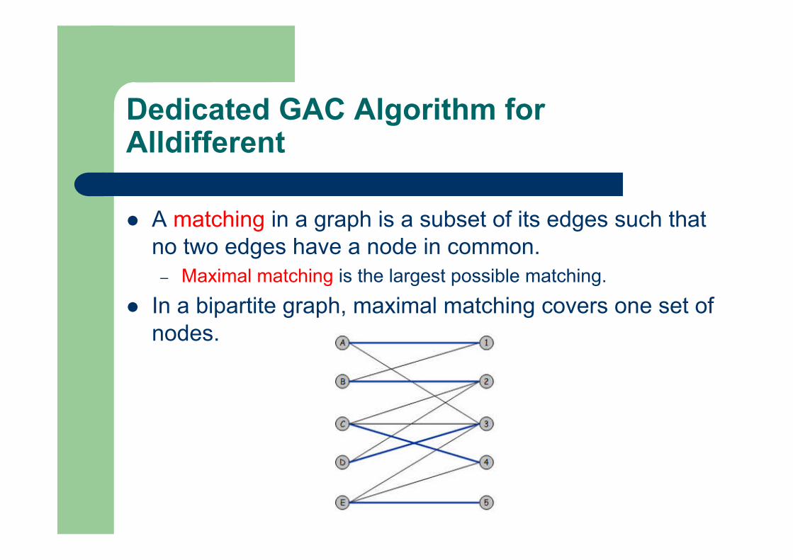
  A matching in a graph is a subset of its edges such that no two edges have a node in common.

–  Maximal matching is the largest possible matching.   In a bipartite graph, maximal matching covers one set of

nodes.


  Observation –  Construct a bipartite graph G between the variables

[X1, X2, …, Xn] and their possible values {1, …, d} (variable-value graph).

–  An assignment of values to the variables is a solution iff it corresponds to a maximal matching in G.   A maximal matching covers all the variables.

–  Use matching theory to compute all maximal matchings efficiently.   One maximal matching can describe all maximal matchings!

Example

Variable-value graph

A First Maximal Matching

Another Maximal Matching

Matching Notations

  Edge: –  matching if takes part in a matching; –  free otherwise.

  Node: –  Matched if incident to a matching edge; –  free otherwise.

  Vital edge: –  belongs to every maximal matching.

Free, Matched, Matching

Algorithm

  Compute all maximal matchings.   No maximal matching exists failure.   An edge free in all maximal matchings

–  Remove the edge. –  Amounts to removing the corresponding value from the domain of the

corresponding variable.   A vital edge

–  Keep the edge. –  Amounts to assigning the corresponding value to the corresponding

variable.   Edges matching in some but not all maximal matchings

–  Keep the edge.

All Maximal Matchings

  Use matching theory to compute all maximal matchings efficiently.

–  One maximal matching can describe all maximal matchings! –  Connection between the edges of one matching and edges

in the other matchings.

Alternating Path and Cycle

  Alternating path –  Simple path with edges alternating free and matching.

  Alternating cycle –  Cycle with edges alternating free and matching.

  Length of path/cycle –  Number of edges in the path/cycle.

  Even path/cycle –  Path/cycle of even length.

Matching Theory

  An edge e belongs to a maximal matching iff: –  For some arbitrary maximal matching M:

  Either e belongs to even alternating path starting at a free node;

  Or e belongs to an even alternating cycle.

  The result is due to Claude Berge in 1970.

Oriented Graph

  As we are interested in even alternating path/cycle, we orient edges of an arbitrary maximal matching for simplicity:

–  Matching edges from variable to value; –  Free edges from value to variable.

An Arbitrary Maximal Matching

Oriented Graph

Even Alternating Paths

  Start from a free node and search for all nodes on directed simple path.

–  Mark all edges on path. –  Alternation built-in.

  Start from a value node. –  Variable nodes are all matched.

  Finish at a value node for even length.



•  Intuition: edges can be permuted.

Even Alternating Cycles

  Compute strongly connected components (SCCs). –  Two nodes a and b are strongly connected iff there is a path

from a to b and a path from b to a. –  Strongly connected component: any two nodes are strongly

connected. –  Alternation and even length built-in.

  Mark all edges in all strongly connected components.



•  Intuition: variables consume all the values.

All Marked Edges

Removing Edges

  Remove the edges which are: –  free (does not occur in our arbitrary maximal matching) and

not marked (does not occur in any maximal matching); –  marked as black in our example.

  Keep the edge matched and not marked. –  Marked as red in our example. –  Vital edge!

Removing Edges

Edges Removed

D(X1) = {0,1}, D(X2) = {1,2}, D(X3) = {0,2}, D(X4) = {3}, D(X5) = {4,5}, D(X6) = {5,6}

Summary of the Algorithm

  Construct the variable-value graph.   Find a maximal matching M; otherwise fail.   Orient graph (done while computing M).   Mark edges starting from free value nodes using

graph search.   Compute SCCs and mark joining edges.   Remove not marked and free edges.   Complexity: O(d2n2.5)

–  O(nd) for SCCs –  O(n1.5d) for computing a maximal matching

Incremental Properties

  Keep the variable and value graph between different invocations.

  When re-executed: –  remove marks on edges; –  remove edges not in the domains of the

respective variables; –  if a matching edge is removed, compute a new

maximal matching; –  otherwise just repeat marking and removal.

Dedicated Algorithms

  Is it always easy to develop a dedicated algorithm for a given constraint?

  There’s no single recipe!   A nice semantics often gives us a clue!

–  Graph Theory –  Flow Theory –  Combinatorics –  Complexity Theory, …

  GAC may as well be NP-hard! –  In that case, algorithms which maintain weaker

consistencies (like BC) are of interest.

GAC for Nvalue Constraint

  nvalue([X1, X2, …, Xn], N) holds iff N = |{Xi | 1 ≤ i ≤ n }|   Reduction from 3 SAT.

-  Given a Boolean fomula in k variables (labelled from 1 to k) and m clauses, we construct an instance of nvalue([X1, X2, …, Xk+m], N):

•  D(Xi) = {i, i’} for i ∈ {1,…, k} where Xi represents the truth assignment of the SAT variables;

•  Xi where i > k represents a SAT clause (disjunction of literals); •  for a given clause like x V y’ V z, D(Xi) = {x, y’, z}.

-  By construction, [X1, …, Xk] will consume all the k distinct values. -  When N = k, nvalue has a solution iff the original SAT problem has a

satisfying assignment. •  Otherwise we will have more than k distinct values. •  Hence, testing a value for support is NP-complete, and enforcing GAC is

NP-hard!

GAC for Nvalue Constraint

  E.g., C1: (a OR b’ OR c) AND C2: (a’ OR b OR d) AND C3: (b’ OR c’ OR d)

  The formula has 4 variables (a, b, c, d) and 3 clauses (C1, C2, C3).   We construct nvalue([X1, X2, …, X7], 4) where:

-  D(X1) = {a, a’}, D(X2) = {b, b’}, D(X3) = {c, c’}, D(X4) = {d, d’}, D(X5) = {a, b’, c}, D(X6) = {a’, b, d}, D(X7) = {b’, c’, d}

  An assignment to X1, …, X4 will consume 4 distinct values.   Not to exceed 4 distinct values, the rest of the variables must have

intersecting values with X1, …, X4.   Such assignments will make the SAT formula TRUE.

Outline




  Decompositions   Ad-hoc algorithms


Generalized Propagation Algorithms

  Not all constraints have nice semantics we can exploit to devise an efficient specialized propagation algorithm.

  Consider a product configuration problem. –  Compatibility constraints on hardware components:

  only certain combinations of components work together. –  Compatibility may not be a simple pairwise relationship:

  video cards supported function of motherboard, CPU, clock speed, O/S, ...

Production Configuration Problem

  5-ary constraint: –  Compatible (motherboard345, intelCPU,

2GHz, 1GBRam, 80GBdrive).) –  Compatible (motherboard346, intelCPU,

3GHz, 2GBRam, 100GBdrive). –  Compatible (motherboard346, amdCPU,

2GHz, 2GBRam, 100GBdrive). –  …

Crossword Puzzle

  Constraints with different arity:

–  Word1 ([X1,X2,X3]) –  Word2 ([X1,X13,X16]) –  …

  No simple way to decide acceptable words other than to put them in a table.

GAC Schema

  A generic propagation algorithm. –  Enforces GAC on an n-ary constraint given by:

  a set of allowed tuples;   a set of disallowed tuples;   a predicate answering if a constraint is satisfied or not.

–  Sometimes called the “table” constraint:   user supplies table of acceptable values.

  Complexity: O(edn) time   Hence, n cannot be too large!

–  Many solvers limits it to 3 or so.

Arc Consistency Algorithms

  Generic AC algorithms with different complexities and advantages:

–  AC3 –  AC4 –  AC6 –  AC2001 –  …

AC-3

  Idea –  Revise (Xi, C): removes unsupported values of Xi

and returns TRUE. –  Place each (Xi, C) where Xi participates to C and its

domain is potentially not AC, in a queue Q; –  while Q is not empty:

  select and remove (Xi, C) from Q;   if revise(Xi, C) then

–  If D(Xi) = { } then return FALSE; –  else place {(Xj, C’) | Xi, Xj participate in some C’} into Q.

AC-3

  AC-3 achieves AC on binary CSPs in O(ed3) time and O(e) space.

  Time complexity is not optimal   Revise does not remember anything about past

computations and re-does unnecessary work.

AC-3

(X, C1) is put in Q

only check of X ← 3 was necessary!

AC-4

  Stores max. amount of info in a preprocessing step so as to avoid redoing the same constraints checks.

  Idea: –  Start with an empty queue Q. –  Maintain counter[Xi, vj, Xk] where Xi, Xk participate in a

constraint Cik and vj ∈ D(Xi)   Stores the number of supports for Xi ← vj on Cik.

–  Place all supports of Xi ← vj (in all constraints) in a list S[Xi, vj].

AC-4

  Initialisation: –  All possible constraint checks are performed. –  Each time a support for Xi ← vj is found, the corresponding counters

and lists are updated. –  Each time a support for Xi ← vj is not found, remove vj from D(Xi) and

place (Xi, vj) in Q for future propagation. –  If D(Xi) = { } then return FALSE.

AC-4

  Propagation: –  While Q is not empty:

  Select and remove (Xi, vj) from Q;   For each (Xk, vt) in S[Xi, vj]

–  If vt ∈ D(Xk) then   decrement counter[Xk, vt, Xi]   If counter[Xk, vt, Xi] = 0 then

  Remove vt from D(Xk); add (Xk, vt) to Q   If D(Xk) = { } then return FALSE.

AC-4

(y,3) is put in Q

No additional constraint

check!

AC-4

  AC-3 achieves AC on binary CSPs in O(ed2) time and O(ed2) space.

  Time complexity is optimal   Space complexity is not optimal

  AC-6 and AC-2001 achieve AC on binary CSPs in O(ed2) time and O(ed) space.

–  Time complexity is optimal –  Space complexity is optimal

PART IV: Search Algorithms

Documents

AIMMS - unibo.itgabbri/MaterialeCorsi/CP-L3.pdf · Solving CSPs Search algorithm. – Usually backtracking search performing a depth-first traversal of a search tree. Local consistency