Embed Size (px)
Citation preview
Air-path control of clean diesel engines : for disturbancerejection on NOx, PM and fuel efficiencyCriens, C.H.A.
DOI:10.6100/IR769972
Published: 01/01/2014
Document VersionPublisher’s PDF, also known as Version of Record (includes final page, issue and volume numbers)
Please check the document version of this publication:
• A submitted manuscript is the author's version of the article upon submission and before peer-review. There can be important differencesbetween the submitted version and the official published version of record. People interested in the research are advised to contact theauthor for the final version of the publication, or visit the DOI to the publisher's website.• The final author version and the galley proof are versions of the publication after peer review.• The final published version features the final layout of the paper including the volume, issue and page numbers.
Link to publication
Citation for published version (APA):Criens, C. H. A. (2014). Air-path control of clean diesel engines : for disturbance rejection on NOx, PM and fuelefficiency Eindhoven: Technische Universiteit Eindhoven DOI: 10.6100/IR769972
General rightsCopyright and moral rights for the publications made accessible in the public portal are retained by the authors and/or other copyright ownersand it is a condition of accessing publications that users recognise and abide by the legal requirements associated with these rights.
• Users may download and print one copy of any publication from the public portal for the purpose of private study or research. • You may not further distribute the material or use it for any profit-making activity or commercial gain • You may freely distribute the URL identifying the publication in the public portal ?
Take down policyIf you believe that this document breaches copyright please contact us providing details, and we will remove access to the work immediatelyand investigate your claim.
Download date: 14. Feb. 2018

Chris Criens
Air-Path Control of Clean Diesel Enginesfor disturbance rejection on NOx, PM and fuel e�ciency
Air-Path Control of Clean D
iesel Engines for disturbance rejection on NOx , PM
and fuel e�ciency
Chris Criens


Air-Path Control of Clean Diesel Enginesfor disturbance rejection on NOx, PM and fuel efficiency

This research was financially supported by the HighTech AutomotiveSystems (HTAS), Further Emission Reduction, Vehicle Efficiency gainsand Neutral Thermal loading (FERVENT) program.
The research reported in this thesis is part of the research program of theDutch Institute of Systems and Control (DISC). The author hassuccessfully completed the educational program of the Graduate SchoolDISC.
Air-Path Control of Clean Diesel Engines for disturbance rejection onNOx, PM and fuel efficiencyby Chris CriensEindhoven: Technische Universiteit Eindhoven, 2014 - Proefschrift
A catalogue record is available from the Eindhoven University ofTechnology Library.ISBN: 978-90-386-3575-0NUR: 951
Typeset by the author using LATEX2eCover design: Chris CriensCover picture: DAF Trucks N.V. Imagebank, PACCAR MX-13 - EURO 6Reproduction: Ipskamp Drukkers B.V., Enschede, The Netherlands
Copyright c©2013 by C.H.A.Criens. All rights reserved.

Air-Path Control of Clean Diesel Enginesfor disturbance rejection on NOx, PM and fuel efficiency
PROEFSCHRIFT
ter verkrijging van de graad van doctor aan deTechnische Universiteit Eindhoven, op gezag van derector magnificus, prof.dr.ir. C.J. van Duijn, voor een
commissie aangewezen door het College voorPromoties in het openbaar te verdedigenop donderdag 13 maart 2014 om 16.00 uur
door
Christiaan Henricus Antonius Criens
geboren te Roermond

Dit proefschrift is goedgekeurd door de promotoren en de samenstellingvan de promotiecommissie is als volgt:
Voorzitter: prof.dr. L.P.H. de Goey
Promotor: prof.dr.ir. M. Steinbuch
Copromotor: dr.ir. F.P.T. Willems
Leden: prof.dr. L. del Re (Johannes Kepler Universität Linz)
prof.dr.ir. J. Schoukens (Vrije Universiteit Brussel)
dr. L. Eriksson (Linköping University)
prof.dr.ir. P.M.J. Van den Hof
Adviseurs: dr.ir. T.A.C. van Keulen

Contents
v
Contents v
Glossary ix
1 Introduction 11.1 Requirements on the Air-Path Control System . . . . . . . . . 61.2 State of the Art of Engine Control . . . . . . . . . . . . . . . 8
1.2.1 Production Engines . . . . . . . . . . . . . . . . . . . . 81.2.2 Literature . . . . . . . . . . . . . . . . . . . . . . . . . 10
1.3 Opportunities for Improvement . . . . . . . . . . . . . . . . . 111.4 Approach . . . . . . . . . . . . . . . . . . . . . . . . . . . . . 121.5 Main Contributions . . . . . . . . . . . . . . . . . . . . . . . . 141.6 Overview of this Thesis . . . . . . . . . . . . . . . . . . . . . 16
2 Fundamentals of Diesel Engines and Combustion 192.1 The EURO VI Engine Layout . . . . . . . . . . . . . . . . . . 19
2.1.1 Fuel Path . . . . . . . . . . . . . . . . . . . . . . . . . 202.1.2 Air Path . . . . . . . . . . . . . . . . . . . . . . . . . . 212.1.3 Exhaust Aftertreatment . . . . . . . . . . . . . . . . . . 22
› Selective Catalytic Reduction . . . . . . . . . . . . . . 23› Diesel Particulate Filter . . . . . . . . . . . . . . . . . 23
2.2 Emission Formation and Fuel Efficiency . . . . . . . . . . . . 242.2.1 Combustion Process . . . . . . . . . . . . . . . . . . . . 242.2.2 Emission Formation . . . . . . . . . . . . . . . . . . . . 26
› Nitrogen Oxides . . . . . . . . . . . . . . . . . . . . . 26› Particulate Matter . . . . . . . . . . . . . . . . . . . . 27

vi
2.2.3 Fuel Efficiency . . . . . . . . . . . . . . . . . . . . . . . 282.2.4 Simultaneously Low NOx, PM and BSFC? . . . . . . . . 31
2.3 Emission Legislation . . . . . . . . . . . . . . . . . . . . . . . 322.3.1 EURO VI Legislation . . . . . . . . . . . . . . . . . . . 34
› Stationary Testing . . . . . . . . . . . . . . . . . . . . 34› Transient Testing . . . . . . . . . . . . . . . . . . . . 35› Not-To-Exceed Tests . . . . . . . . . . . . . . . . . . . 35› In-Service Conformity . . . . . . . . . . . . . . . . . . 37› Implications for Engine Design and Control . . . . . . . 38
3 Literature Overview 413.1 Controlled Outputs . . . . . . . . . . . . . . . . . . . . . . . . 42
3.1.1 Track Boost Pressure and Fresh Air Flow . . . . . . . . . 423.1.2 Minimize NOx Emissions . . . . . . . . . . . . . . . . . 433.1.3 EGR Rate and Air-Fuel Ratio . . . . . . . . . . . . . . . 443.1.4 Direct Emission Control . . . . . . . . . . . . . . . . . . 45
3.2 Model Predictive Control . . . . . . . . . . . . . . . . . . . . 463.3 Transient Control . . . . . . . . . . . . . . . . . . . . . . . . . 503.4 Discussion . . . . . . . . . . . . . . . . . . . . . . . . . . . . . 52
4 Modeling, Identification and Analysis 594.1 Introduction . . . . . . . . . . . . . . . . . . . . . . . . . . . . 594.2 Measurement Setup . . . . . . . . . . . . . . . . . . . . . . . . 63
4.2.1 Engine . . . . . . . . . . . . . . . . . . . . . . . . . . . 634.2.2 Actuators . . . . . . . . . . . . . . . . . . . . . . . . . 644.2.3 Sensors . . . . . . . . . . . . . . . . . . . . . . . . . . 64
4.3 Design of the Input Signal . . . . . . . . . . . . . . . . . . . . 654.3.1 Multisine . . . . . . . . . . . . . . . . . . . . . . . . . 654.3.2 Influence of Input Quantization . . . . . . . . . . . . . . 68
4.4 Analysis of the Identification Accuracy . . . . . . . . . . . . . 694.4.1 Frequency Response Function . . . . . . . . . . . . . . . 714.4.2 Accuracy of the Frequency Response Function . . . . . . 724.4.3 Classification of Nonlinearities . . . . . . . . . . . . . . 744.4.4 Time-Domain Validation . . . . . . . . . . . . . . . . . 77
4.5 Frequency Response Function Measurement Results . . . . . . 824.6 Discussion . . . . . . . . . . . . . . . . . . . . . . . . . . . . . 854.7 Conclusions . . . . . . . . . . . . . . . . . . . . . . . . . . . . 86

vii
5 Feedback Control for Disturbance Rejection 895.1 Introduction . . . . . . . . . . . . . . . . . . . . . . . . . . . . 895.2 Control Problem . . . . . . . . . . . . . . . . . . . . . . . . . 905.3 Conceptual Design . . . . . . . . . . . . . . . . . . . . . . . . 93
5.3.1 Actuators . . . . . . . . . . . . . . . . . . . . . . . . . 935.3.2 Controlled Outputs . . . . . . . . . . . . . . . . . . . . 955.3.3 Input-Output Controllability . . . . . . . . . . . . . . . 965.3.4 Control Design . . . . . . . . . . . . . . . . . . . . . . 965.3.5 Simulation Result . . . . . . . . . . . . . . . . . . . . . 97
5.4 Experimental Design . . . . . . . . . . . . . . . . . . . . . . . 1025.4.1 Selection of Controlled Outputs . . . . . . . . . . . . . . 1025.4.2 Input-Output Analysis . . . . . . . . . . . . . . . . . . 1075.4.3 Control Design . . . . . . . . . . . . . . . . . . . . . . 111
› Decoupling . . . . . . . . . . . . . . . . . . . . . . . . 112› Feedback Control Design . . . . . . . . . . . . . . . . 113
5.4.4 Experimental Results . . . . . . . . . . . . . . . . . . . 117
6 Control on the Full Speed-Load Range 1256.1 Feedback Control . . . . . . . . . . . . . . . . . . . . . . . . . 127
6.1.1 NOx Measurement . . . . . . . . . . . . . . . . . . . . . 1286.1.2 Decoupling . . . . . . . . . . . . . . . . . . . . . . . . 1296.1.3 PI control . . . . . . . . . . . . . . . . . . . . . . . . . 1326.1.4 Implementation . . . . . . . . . . . . . . . . . . . . . . 134
› Nominal Inputs and Setpoint Values . . . . . . . . . . 134› Safety . . . . . . . . . . . . . . . . . . . . . . . . . . 135
6.1.5 Experimental Results . . . . . . . . . . . . . . . . . . . 1366.2 Feed-Forward Control . . . . . . . . . . . . . . . . . . . . . . 138
6.2.1 Control Design . . . . . . . . . . . . . . . . . . . . . . 1406.2.2 Tuning Process . . . . . . . . . . . . . . . . . . . . . . 1416.2.3 Torque Step Experiments . . . . . . . . . . . . . . . . . 143
6.3 Experimental WHTC Tests . . . . . . . . . . . . . . . . . . . 145
7 Conclusions & Recommendations 1517.1 Conclusions . . . . . . . . . . . . . . . . . . . . . . . . . . . . 151
7.1.1 Disturbance Rejection . . . . . . . . . . . . . . . . . . . 1517.1.2 Design Effort . . . . . . . . . . . . . . . . . . . . . . . 1527.1.3 Summary of the Main Results . . . . . . . . . . . . . . . 153
› Identification . . . . . . . . . . . . . . . . . . . . . . . 153
viii
› Disturbance Rejection . . . . . . . . . . . . . . . . . . 154› Full Operating Range . . . . . . . . . . . . . . . . . . 155
7.2 Recommendations for Future Research . . . . . . . . . . . . . 1567.2.1 Improved Air Path Control . . . . . . . . . . . . . . . . 156
› Control Algorithm . . . . . . . . . . . . . . . . . . . . 156› Controlled Outputs . . . . . . . . . . . . . . . . . . . 157› Experiments . . . . . . . . . . . . . . . . . . . . . . . 158› Transients . . . . . . . . . . . . . . . . . . . . . . . . 158
7.2.2 Modeling . . . . . . . . . . . . . . . . . . . . . . . . . 1597.2.3 Integrated Engine Control . . . . . . . . . . . . . . . . . 160
Bibliography 163
Summary 171
Samenvatting 175
Dankwoord 179
Curriculum Vitae 183

Glossary
ix
ACEA Association des Constructeurs Européens d’Automobiles; English: Euro-pean Automobile Manufacturers Association
AFR Air-Fuel Ratio
AMOX AMmonia OXidation catalyst
a.u. arbitrary units
AVL Anstalt für Verbrennungskraftmaschinen List
BDC Bottom Dead Center
BLA Best Linear Approximation
BMEP Brake Mean Effective Pressure
BPV Back Pressure Valve
BSFC Brake Specific Fuel Consumption
CA50 Crank Angle at which 50% of the combustion heat is released
CO Carbon monoOxide
CO2 Carbon diOxide
CR Common-Rail
DFT Discrete Fourier Transform
DOC Diesel Oxidation Catalyst
DOE Design Of Experiments
DPF Diesel Particulate Filter
ECE R49 Regulation No. 49 of the Economic Commission for Europe
ECU Engine Control Unit

x
EEA European Environment Agency
EGR Exhaust Gas Recirculation
ESC European Stationary Cycle
ETC European Transient Cycle
EU European Union
FERVENT Further Emission Reduction, Vehicle Efficiency gains and NeutralThermal loading
FRF Frequency Response Function
HC Hydro Carbons
HCCI Homogeneous Charge Compression Ignition
HD Heavy Duty
HTAS HighTech Automotive Systems
IDFT Inverse Discrete Fourier Transform
IJPT International Journal of PowerTrains
IMC Internal Model Control
IMEP Indicated Mean Effective Pressure
FMEP Friction Mean Effective Pressure
LPV Linear Parameter Varying
LQG Linear Quadratic Gaussian
LTC Low Temperature Combustion
LTI Linear Time Invariant
MAF fresh Mass Air Flow
MAP Manifold Absolute Pressure, (also: Manifold Air Pressure)
MIMO Multi-Input Multi-Output
MISO Multi-Input Single-Output
MPC Model Predictive Control
NEDC New European Driving Cycle
NL NonLinear
NMHC Non-Methane Hydro Carbons
NOx Nitrogen Oxides

xi
OBD On-Board Diagnostics
ODE Ordinary Differential Equations
PCCI Premixed Charge Compression Ignition
PC Personal Computer
PEMS Portable Emission Measurement System
PI Proportional Integral controller
PID Proportional Integral Derivative controller
PM Particulate Matter
PMEP Pumping Mean Effective Pressure
PN Particle Number
ppm parts per million
RGA Relative Gain Array
RMS Root Mean Square
RPM Revolutions Per Minute
SCR Selective Catalytic Reduction
SISO Single-Input Single-Output
SOI Start Of Injection
SVD Singular Value Decomposition
SQP Sequential Quadratic Programming
TDC Top Dead Center
THC Total HydroCarbon
TITO Two-Input Two-Output
TNO Nederlandse organisatie voor Toegepast-Natuurwetenschappelijk Onderzoek
TU/e Eindhoven University of Technology
UEGO Universal Exhaust Gas Oxygen
US United States
VGT Variable Geometry Turbine
WNTE World-harmonized Not-To-Exceed
WHSC World-Harmonized Steady-state Cycle
WHTC World Harmonized Transient Cycle


1 Introduction
1
The goal of this research is to design a control system for heavy-duty diesel enginesthat is capable of combining a low fuel consumption with low emissions of NitrogenOxides (NOx) and Particulate Matter (PM). In addition, these properties shouldbe maintained when disturbances are present. A feature of the to be designedcontrol system should be that the required design effort is low. The relevance ofsuch a control system is further detailed in this introduction.
Fuel efficiency and reliability made diesel engines the most popular meansof propulsion for commercial Heavy-Duty (HD) trucks. In spite of their fuelefficiency and accordingly low CO2 emissions, diesel engines are known to causemore pollution than gasoline engines (Guzzella and Amstutz, 1998). The leandiffusion combustion in diesel engines produces more PM and makes the use ofthree-way catalysts ineffective, resulting in higher NOx emissions.
The 2013 report of the European Environment Agency (EEA) on emissions inthe European Union (EU) between 1990 and 2011 (European Environment Agency,2013), provides data on the recent evolution of harmful emissions in the EU. Roadtransport is one of the main contributors to these emissions. In 2011, 40% ofthe total NOx emissions originated from road transport, equally divided betweenpassenger cars and commercial HD vehicles. Also, 17% of the total fine PMemissions originated from road transport, slightly more from passenger cars thanfrom HD vehicles. To protect man and his environment against the air pollutioncaused by these emissions, the EU restricts these emissions via legislation. As aresult, the total emissions of NOx decreased with 48% between 1990 and 2011.For the PM emissions, a 20% reduction was achieved between 2000 and 2011. The

2 Chapter 1. Introduction
’92
’96’98’00
’05
’08
’13
00.42
3.55
78
0 20
100150
250
360
’92
’96’98’00
’05
’08
’13
PM in mg/kWh NOx in g/kWh
EURO I
EURO IIa
EURO IIb
EURO III
EURO IV
EURO V
EURO VI
Figure 1.1: The evolution of the heavy-duty steady-state emission limits for NOxand PM in the European Union. Data source: DieselNet (2013).
EU goal for 2020 is to achieve a further 42% and 22% decrease in the overall NOx
and PM emissions, respectively, with the 2005 emissions as the baseline.
Figure 1.1 shows the evolution of the limits for NOx and PM emissions ofHD diesel engines in the European Union. With EURO VI, the emission limitshave reached near zero impact levels. Moreover, to increase the practical impactof the tightened legislation, World harmonized Not-To-Exceed (WNTE) and in-service conformity emission limits are introduced with EURO VI (see Section 2.3.1for more details). The drive cycle, ambient conditions, fuel composition, produc-tion tolerances and ageing can all influence the produced emissions. This makesguaranteeing compliance with in-service emission limits particularly challenging.
Considering the NOx and PM emission goal for 2020, the low emission limitsin EURO VI and the natural phasing out of EURO III, EURO IV and EURO Vvehicles, further drastic cuts in the allowed emission levels are not expected inthe near future. Instead, legislation restricting the CO2 emissions, or almostequivalently, the fuel consumption, is anticipated. In the United States (US), fuelconsumption legislation for 2014-2018 engines is already finalized. Up until theintroduction of increasingly stringent emission legislation, a trend was observed

Chapter 1. Introduction 3
that fuel economy improved in newer vehicles. Because reducing the emissionsof NOx and PM required the implementation of measures that conflict with fuelefficiency, this trend has stopped, despite the advancements in technology. Fuelconsumption is, and has been, a major competitive factor for truck manufacturers.Any cost effective solution to reduce the fuel consumption is therefore readilyadopted in production vehicles (ACEA, 2010). When needed for compliance withlegislation, fuel-reduction technologies that have not proven to be cost-effectivewill be implemented as well.
For engine manufacturers, the increasingly stringent legislation requires con-stant innovation of their engines. Complying with emission legislation in a costeffective manner and with minimum impact on the fuel consumption, resulted inthe adoption of several new hardware components. A typical EURO VI enginecomprises components that provide control over the air intake and fuel injection,and reduce the emissions via exhaust gas aftertreatment. Figure 1.2 lists thecomponents typically available in a modern EURO VI HD diesel engine.
To utilize the flexibility provided by the new components and release theirfull potential, a digital, electronic control system is used. This system providessettings for each component, based on the actual engine speed, torque demand andsensor measurements. Along with the increase in the number of components, thecomplexity of this control system increased as well. The time and effort needed todesign and calibrate a control system that achieves optimal, or at least satisfactory,engine performance increased significantly.
In this thesis, control design for the diesel engine air path is considered. Air-path control is particularly interesting. It is challenging and time consuming tocalibrate using current control methods. Moreover, the air path contains a varietyof sensors and actuators, which means that within the current hardware constraints,various control layouts are possible. The main actuators in the air path are theVariable Geometry Turbine (VGT) and Exhaust Gas Recirculation (EGR) valve.Figure 1.3 shows the air path of an EGR diesel engine including a VGT and EGRvalve.
Exhaust Gas Recirculation (EGR) is used in diesel engines to reduce the NOx
emissions. By diluting the intake air with cooled exhaust gas, the combustiontemperature is lowered, which reduces the NOx formation. The combination of a

4 Chapter 1. Introduction
Fuel PathCommon Rail System
• Rail pressure
• Pilot injection (number, quantity, timing)
• Main injection (quantity, timing)
• Post injection (number, quantity, timing)
Air PathEngine with Exhaust Gas Recirculation (EGR)
• EGR system, with EGR valve and EGR cooler
• VGT, with charge air cooler
• Intake throttle, back pressure valve
ExhaustAftertreatment Systems
• Diesel Oxidation Catalyst (DOC)
• Selective Catalytic Reduction (SCR) for NOx reduction
• Diesel Particulate Filter (DPF) for PM reduction
• AMmonia OXidation (AMOX) catalyst for NH3 reduction
Engine
Figure 1.2: Subsystems of a typical, heavy-duty EURO VI engine.
EGRcooler
Aircooler
pin
pex
EGRvalve
VGT
NOx
λ
Com-pressor
Intake manifold
Exhaust manifold
Fresh airMAF
Dynamo-meter
fuel
Exhaust gas
Figure 1.3: A schematic representation of the layout of the air path of the studiedEGR engine.

Chapter 1. Introduction 5
VGT and EGR valve provides control over the flows of fresh air and exhaust in theengine. This affects the NOx and PM emissions as well as the fuel efficiency. Moredetails on the functioning of the VGT and EGR are provided in Section 2.1.2.
For EURO VI, emission control has gained importance. The allowed emissionlimits were drastically reduced, which makes tight compliance with legislationincreasingly important to minimize the fuel consumption. Moreover, to ensurein-service conformity, which is required for EURO VI, the effects of disturbancesand uncertainties in the engine have to be accounted for. Via the VGT and EGRvalve actuators, the air-path controller affects the NOx and PM emissions and thefuel consumption. The air-path controller is therefore a key part of the design of afuel efficient, EURO VI compliant diesel engine.
Air-path control for diesel engines is considered challenging. Several conflictingand tight requirements are present (Alberer et al., 2012). Minimizing the engine-out NOx emissions can result in excessive PM emissions and vice versa. Toachieve EURO VI compliance, both emission species must be mainted within tightbounds. To be economically viable, the fuel consumption must be minimized. Thedynamic behavior of the air path can be characterized as coupled, nonlinear andnonminimum phase. These characteristics complicate control design. Also, theexternal disturbances and internal uncertainties that are present affect both theoutputs of the system and the dynamic input-output response. A successful controldesign should have regard for all the above aspects.
The use of EGR, controlled via the EGR valve and VGT, is not limited tocurrent EURO VI engines. Advanced combustion concepts such as Low Tempera-ture Combustion (LTC), Homogeneous Charge Compression Ignition (HCCI) andPremixed Charge Compression Ignition (PCCI) also rely heavily on the use ofEGR. Engines using these combustion concepts are currently being investigated inacademic literature. They have the potential to combine extremely low emissionswith a high fuel efficiency. In particular for HCCI and PCCI engines, very highEGR rates are necessary for proper functioning. EGR is used to reduce the oth-erwise excessive combustion rate and can also be used to control the combustionphasing. For these engines, control is even more important than for the EUROVI diesel engines considered in this thesis. Their operation is not naturally stable,which makes the use of feedback control a necessity.

6 Chapter 1. Introduction
1.1 Requirements on the Air-Path Control System
The main purpose of a diesel engine in a commercial vehicle is to provide propulsion.The control system provides some essential tasks in achieving this in the best waypossible.
On a high level, the goals of a diesel engine control system are as follows.
• Drivability Achieve a satisfactory level of drivability, i.e., comply with thedrivers torque demand.
• Legislation Comply with the EURO VI emission legislation, both for typeapproval and in use.
• Fuel consumption Minimize the operational costs of the vehicle, which arelargely determined by the fuel consumption.
• Constraints Remain within limits for safety, noise and durability.
The control system is not the only factor that determines whether or not theabove goals are met. The synergy between the engine hardware, its control systemand the external conditions determines the achieved engine performance. As asubsystem of the overall engine control system, the air-path controller can providea partial contribution to achieving the above goals. The following list provides themain aspects where the air-path controller can contribute.
• Enable overall low emissions and low fuel consumption The air pathaffects the engine-out NOx and PM emissions as well as the fuel efficiency.The air-path controller should therefore apply settings that result in simulta-neously low NOx and PM emissions and a low fuel consumption.
• Improve the robustness The real-world emissions of a diesel engine areaffected by disturbances and uncertainties such as ambient conditions, fuelcomposition, production tolerances and ageing. In particular for EURO VIengines, where not-to-exceed and in-service conformity limits are enforced,reducing the effects of these disturbances and uncertainties on the NOx
and PM emissions is important for tight compliance with the limits set inlegislation.

1.1. Requirements on the Air-Path Control System 7
• Decrease the turbo lag The turbocharger is responsible for providing thefresh air flow that is required to generate a high brake torque. When thetorque demand is low, the turbocharger speed is low as well. Due to itsinertia, the turbocharger cannot instantly speed up and provide the boostpressure and air flow needed to generate the peak torque. Consequently,when the driver demands a fast change from low to high torque, turbo lagis observed, while the turbocharger speeds up. In an engine equipped witha VGT and EGR system, the EGR flow and pressures in the intake andexhaust manifold can be influenced by the VGT and EGR valve. This canresult in a faster acceleration of the turbine and an additional increase in thefresh air flow ahead of the increase in turbine speed. Control using the VGTand EGR valve therefore affects the observed turbo lag.
The control design in this thesis focusses on performance with respect to theabove aspects. For a practical integration into a production engine, other aspectsare relevant as well.
• Design time An increase in the design time and effort results in an increasein the costs associated with control design. Moreover, the time to market ofnew engines increases. The increase in flexibility due to additional actuatorsand sensors resulted in a significant increase in control design effort. It iseven expected that by 2020, the effort associated with control design exceedsthe effort associated with the design of the engine hardware. Consideringthis, the effort needed for control design is a considerable factor to take intoaccount.
• Computational complexity The computational power of a modern EngineControl Unit (ECU) and the memory available for storage are limited. Thefootprint on the ECU should therefore be small and be compatible withcurrent production ECUs.
• Use currently available hardware Research engines can be equipped withan extensive sensor set and additional actuators. In production engines, themeans are much more limited. Size, cost-effectiveness and reliability limit theavailability of sensors and actuators and a control design should fit withinthese restrictions.

8 Chapter 1. Introduction
• Flexibility Engines will have different modes that are selected depending onthe current requirements, e.g., during warm-up, the engine will be controlleddifferently than during normal operation. A control system should be ableto cope with this and remain functional.
• General applicability The control design method should be applicable fora range of engine topologies. Moreover, the controller should work withoutfurther modification on a full production series during the complete live cycleof the engines.
• Integration into the control system As shown in Figure 1.2, the air-pathcontrol system constitutes only a part of the engine control system. Inconsequence, a synergy with the other parts of the control system is required.
The practical considerations above are important and will be kept in mindduring control design. Compliance with these aspects is flexible, e.g., when asignificant improvement of the fuel efficiency can be achieved, a failure to meetany of the above practical aspects may be justified.
1.2 State of the Art of Engine Control
1.2.1 Production Engines
The control systems that are used in production engines are typically confidentialand undisclosed. The details of the state-of-the-art control systems as applied inproduction engines are therefore not available.
It is however known that production control systems rely heavily on so calledengine maps (Stewart et al., 2010) to control the engine. These maps providesettings for all actuators depending on the speed-load operating point of the engine.By means of Design Of Experiment (DOE), they can be calibrated efficiently. Also,when using a nominal engine, under nominal and steady-state conditions, an enginemap is a nonconservative control method, i.e., under these conditions control viaa well-calibrated engine map is sufficient to achieve optimal performance.
When disturbances are present or the engine is in a transient state, i.e., theengine speed or torque is not constant, an engine map that provides settings based

1.2. State of the Art of Engine Control 9
on the operating point is no longer sufficient for optimal performance. Therefore,additional maps are implemented that adapt the base engine map using sensormeasurements as input. Although they are based on sensor data, the adaptationsare usually of the feed-forward type, i.e., the sensor measurement is not directlyaffected by the actuator setting that is adapted. This type of control designcan theoretically be nonconservative. Suppose that all engine states, externaldisturbances and uncertain parameters are accurately measured. And also thatbased on all these measurements, a multidimensional map is created that containsthe optimal settings for each actuator. This type of control is nonconservative andoptimal performance is achieved.
In a practical setting, achieving optimal performance using the method de-scribed above is not a feasible approach. First of all, not all measurements that aretheoretically required are available. But also, the control design effort will be enor-mous. For example, even using only five internal and three external measurements,and a grid density of 10 control settings per measurement, a total of 108 actuatorsettings have to be calibrated and stored for each actuator. The exponential in-crease in the complexity when the number of measurements or actuators increasesmakes this method of control prohibitively complex, when optimal performance isstrived for.
To reduce the control design effort, subsystems are identified that are calibratedindividually, largely neglecting possible interactions. This reduces the complexity,but also introduces conservatism. Despite this, the control design effort is immense(Stewart et al., 2010; Pachner et al., 2012; Henningsson, 2012; Guzzella and Am-stutz, 1998). Moreover, when sensors and actuators are added to the engine, thecomplexity rapidly increases even further.
In addition to map-based feed-forward control, feedback control is also appliedin production engines. Feedback control can make the achieved performancemore robust against disturbances. Also, feedback control can be an effective wayof reducing the performance requirements on the feed-forward control system,because it can compensate for the remaining inaccuracies. This potentially reducesthe required calibration effort. Details of the applied feedback strategies are notdisclosed. Considering the increasing design time that is widely reported, it canbe concluded that thus far, a feedback control solution that provides a reductionin calibration effort and accurate disturbance compensation is not available.

10 Chapter 1. Introduction
1.2.2 Literature
In literature, diesel engine control and also air-path control are extensively studied.A brief review is presented here, with a more elaborate version in Chapter 3.To determine the state of the art in current academic research on control usingthe VGT and EGR valve, two paths are distinguished. First, the use of newcontrol algorithms is proposed to make control design more efficient, improve onthe achieved performance, or both. Second, the use of new control problems withdifferent output combinations, often using different, newly available sensors isproposed. This results in new control problems that may better reflect the actualhigh-level objectives as listed in Section 1.1. Generally, the use of feedback controlis widespread in academic literature.
In terms of control schemes used for air-path control, the current state of theart is arguably Model Predictive Control (MPC). Several versions of MPC forair-path control have been proposed as listed in Section 3.2. MPC allows for a sys-tematic and optimal control design procedure that can take into account nonlinearsystem behavior, and constraints on the actuator range and internal engine states.This makes MPC very suitable for air-path control from a performance perspective.In consequence of the complexity of the MPC algorithm, several simplifications areneeded to enable an experimental demonstration on an engine. These simplifica-tions complicate the control design and can hamper the performance obtained bythe controller. The differences between the papers listed in Section 3.2 are mostlyfound in the simplifications that are used. Variations are found in the consideredconstraints, the modeling method used to take into account the nonlinear enginebehavior, prediction and control horizon, and the algorithm used to synthesize thecontroller.
The studied control problems found in literature evolve towards more directcontrol of emissions. Initially control designs used control of fresh Mass Air Flow(MAF) and Manifold Absolute Pressure (MAP). Sensors to measure these quantitiesare present by default in the air path of a production engine. Sensors for measuringPM emissions are lacking in current HD production engines, and the use of aNOx sensor is often dismissed due to the slow sensor dynamics of the availableNOx sensors. Direct control of NOx and PM (using a research opacity sensor todetermine PM) is used in Tschanz et al. (2013). Earlier works often also thrivetowards direct emission control, but use substitute measurements, e.g., EGR rate

1.3. Opportunities for Improvement 11
instead of NOx, and λ instead instead of PM. In terms of controlled outputs,a very elaborate study is done in Karlsson et al. (2010), where Indicated MeanEffective Pressure (IMEP), combustion phasing, maximum pressure derivative,NOx emissions and exhaust opacity are controlled. This work also employs MPCcontrol, but in a simplified linear version, which is applicable only at a singlespeed-load operating point.
1.3 Opportunities for ImprovementWith the goals of this research in mind: enable low average emissions and a lowaverage fuel consumption, improve the robustness and decrease the turbo lag.And also considering the current issues with the high control design effort, thestate-of-the-art is reviewed to distinguish opportunities for improvement.
In terms of performance potential, MPC is a very suitable control technology.Moreover, it is very flexible in terms of modeling and can work with a wide range ofoptimization criterions. However, with robustness as a main goal, MPC falls short.Stability, or robust stability, a basic aspect of any practical control algorithm, isnot guaranteed by default. Moreover, the approaches presented in the literatureshow that the computational complexity of the resulting control law pushes theboundaries of what is possible with current ECU hardware. Considering this, thepresented MPC approaches are not very suitable to reduce the control design effortin a practical setting. A systematic, low-complexity control design is likely toimprove upon this.
In terms of the considered outputs, is has been shown that the classical ap-proach of MAF-MAP control is not effective for disturbance rejection on theengine-out NOx and PM emissions. Even high-end control algorithms that achieveaccurate tracking of MAF-MAP do not necessarily improve the performance onthe high-level objectives. In Chapter 5 of this thesis, it is shown that control ofNOx and PM, using the air-path actuators, is not compatible with robust stabilityand may deteriorate the fuel efficiency in a low emission engine. Control solutionsthat take into account both fuel efficiency and emissions are scarce in literature,with Henningsson (2012) and Wahlström et al. (2010) as the main contributions.The work of Henningsson (2012) is intended as an academic showcase and is notsuitable for implementation due to the control algorithm and the use of sensors

12 Chapter 1. Introduction
ENGINE
uVGT
uEGR
u0
ufb
uff
FeedbackControl
DynamicFeed Forward
Steady-StateEngine Map
Operating Point
Sensors
Setpoints
Fuel Path
Air Path
Exhaust
Figure 1.4: An overview of the proposed control scheme.
that are available only on research engines. The work of Wahlström et al. (2010)does not use the currently available emission sensors and aims mostly to minimizethe pumping work. Disturbance rejection on NOx and PM emissions as well asfuel efficiency can improve on the current approaches found in literature.
1.4 ApproachThe control structure that is proposed in this thesis consists of three parts. First,a base engine map defining nominal VGT and EGR settings based on engine speedand torque request, and corresponding setpoints. Second, a feedback controllerto reduce the effects of disturbances. Third, a dynamic feed-forward controller toimprove the torque response and reduce the PM emissions during torque transients.This control layout is illustrated in Figure 1.4.
The steady-state engine map, which is a map with input settings, u0, for allspeed-load operating points, is available a priori and its design is not discussed inthis work. Although it largely determines the actual performance of the engine,standard Design Of Experiments (DOE) techniques are adequate to calibrate theparameters in the engine map. Using DOE, optimal settings for stationary enginespeed and load can be found in a reasonable amount of time. Feed-forward bymeans of a map is very flexible and, when a dense enough grid is used, it isnonconservative for stationary performance under nominal conditions.
The feedback controller is the main part of the new control design. Its purposeis to adapt the VGT and EGR valve, such that the optimal tradeoff between

1.4. Approach 13
NOx, PM and fuel efficiency is maintained as closely as possible when disturbancesare present. Moreover, the feedback controller keeps the NOx and PM emissionsclose to their nominal values, to ensure tight compliance with emission legislation.By applying feedback control, the effects of uncertainties and disturbances arecompensated for. The external disturbances include, e.g., ambient changes intemperature, pressure and humidity, and differences in fuel quality and composi-tion. Also, engine temperature variations, aging, production tolerances, fouling ofthe engine and aftertreatment system, and actuator imperfections and hysteresisaffect the achieved emissions and fuel efficiency. To make feedback control mosteffective, outputs are selected that are directly related with the high-level objec-tives. The NOx emissions, PM emissions and fuel efficiency are represented byNOx emissions, air-fuel equivalence ratio, λ, and pressure difference between theintake and exhaust manifold, ∆p, respectively. The output value that is obtainedunder nominal conditions is used as a setpoint value. When the feedback controlleractively maintains the outputs close to their respective setpoint values, the effectsof changing conditions on the emissions and fuel efficiency is counteracted. Thedesign of the feedback controller is further discussed in Chapter 5.
During transient engine operation, the combination of the engine map withfeedback control is no longer sufficient. To ensure a fast torque response and reducethe PM emissions when a large increase in torque demand is applied, additionalfunctionality is needed. For this reason a dynamic feed-forward controller isimplemented. This controller takes additional control actions based on the variationof the torque demand. This speeds up the response of the fresh air flow and turbinespeed. A simple structure with a small number of parameters is used such thatmanual tuning on a dynamometer test setup is possible. With the extensiveemission measurement capabilities available on a dynamometer setup, the feed-forward parameters can be calibrated to achieve a desirable combination of NOx
emissions, PM emissions and torque response.
Apart from the performance of the controller, the design effort is also a bottle-neck in the design process. Both the proposed feedback controller and feed-forwardcontroller require a short design time. The design of the feedback controller iscompletely model based. This shifts the design effort from manual calibration onan engine towards model design and identification. The multisine identificationprocedure elaborated in Chapter 4 offers a time-efficient identification procedure.

14 Chapter 1. Introduction
The resulting linear Frequency Response Function (FRF) models are directly suit-able for the design of the proposed feedback controller. Moreover, the identificationprocedures allows an extensive analysis of the accuracy of the identified models.The effects of nonlinearities and noise are quantified separately, which providesconfidence in the accuracy of the resulting models and identification procedure.Based on the FRF models, a control design consisting of decoupling and classicalcontrol design is proposed. It is shown that despite the nonlinear behavior, a linearcontroller is effective. This results in a feedback controller with both a low designand implementation effort. The calibration of the dynamic feed-forward controlleris performed manually on a dynamometer test setup. Here, the design effort is lowdue to the small number of parameters (four) that require calibration.
1.5 Main Contributions
The main contributions of this work are: a new feedback and feed-forward controldesign method; multisine FRF identification and analysis applied to the dieselengine air path; a representative testing procedure. To achieve a reduction inthe control design time, this aspect is taken into consideration in all parts of thecontrol design process. This is explained below in more detail.
• New feedback control strategy A new choice of controlled outputs ismade. The NOx sensor, λ sensor are combined with a measurement ofthe pressure difference between intake and exhaust manifold, ∆p. Theseoutputs have a direct relation with the performance measurements of a dieselengine. This selection is aimed at improving the robustness of the engine.Robustness has two interpretations in this context. First, maintaining closed-loop stability in case of uncertainty of the input-output response. Second,maintaining the performance (emissions, fuel consumption, torque response)when disturbances are present. Both aspects of the robustness improve as aresult of this selection. It is shown that with this new selection of controlledoutputs, a linear feedback controller can be used in almost the completeoperating range. This is a significant simplification over alternative controlmethods, which reduces the complexity of the controller and reduces thedesign time.

1.5. Main Contributions 15
• New feed-forward control strategy The feed-forward controller has a newstructure, which is efficient to implement and easy to calibrate. A dynamome-ter test setup that is equipped with emission measurement equipment andtorque sensors is used during calibration. Using a small number of parame-ters, manual tuning for optimal performance is possible. Combined with themeasurement equipment available on a dynamometer setup, direct optimiza-tion of the high-level objectives can be achieved. Compared with previousapproaches, the design complexity and possibility for direct optimization ofthe high level objectives are improvements.
• Time-efficient and accurate system identification Linear system identifi-cation using multisine excitation signals was used to model the input-outputdynamics. The local behavior and accuracy of the identification were exten-sively analyzed. This analysis includes the ability to quantify to what extentthe local behavior is linear. Moreover, the effects of noise and nonlinearityare separated from the identified models and individually quantified. It wasfound that using 10 minutes of measurement time, an accurate local modelcan be identified at a single speed-load operating point. The identified modelsnaturally include both sensor and actuator dynamics, which is importantfor the intended application: the design of feedback controllers. Also, theability to model any measured output, including emissions, is an advantage;the emissions are very difficult to model using first-principles models. Boththe multisine FRF identification procedure and the analysis are not found inliterature for the application of engine control. Moreover, when the operatingpoint is fixed, the accuracy of the resulting models is very high, comparedwith alternative modeling approaches found in literature.
• Representative testing procedure The control design presented in thisthesis is demonstrated and tested experimentally on a EURO VI type engine.The performance is validated while additional disturbances are applied aswell as using the World Harmonized Transient Cycle (WHTC). This cycleis designed to be a realistic representation of actual world-wide usage ofengines in commercial vehicles and is also used in the EURO VI emissiontest procedure. Although in industrial practise the use of realistic test cyclesis common, in academia, controllers are often evaluated on simplified testcycles only.

16 Chapter 1. Introduction
1.6 Overview of this ThesisThe remainder of this thesis is organized as follows.
Chapter 2 contains background information regarding diesel engines and inparticular emission formation and legislation.
In Chapter 3, an overview and review of relevant academic literature in thefield of air-path control and diesel engine control is presented.
Chapters 4 considers modeling, identification and analysis of the dynamicbehavior of the air-path. The chapter elaborates on the identification procedure,accuracy of the resulting models and sources of distortion. The contents of thischapter are also submitted for journal publication.
Chapter 5 deals with feedback control for disturbance rejection around asingle speed-load operating point. The purpose of this controller is to reduce theeffect that disturbances and uncertainties have on the achieved emissions and fuelefficiency. In this chapter, the selection of both sensors and actuators is discussed.Also, the properties of the control problem are analyzed. A feedback controller isdesigned and its ability to counteract disturbances is experimentally validated.
In Chapter 6, the design procedure of a controller to be used with varyingengine speed and load is detailed and executed. The results of Chapter 4 andChapter 5 are used and in addition a dynamic feed-forward controller is designed.The resulting controller is suitable for transient operation in the complete speed-load operating range. A time efficient design process is an important considerationfor the controller in this chapter. The performance of the engine using this controlleris evaluated on the WHTC.
The thesis ends with conclusions and directions for future research. Thepresented control design and performance are reviewed and suggestions for furtherimprovements are provided. Also, suggestions for further integration of the air-pathcontroller into the engine control structure are made.


2 Fundamentals of DieselEngines and Combustion
19
This chapter details the working principles of a modern diesel engine. The layoutof a modern HD EURO VI diesel engine is described in Section 2.1. Section 2.2is dedicated to diesel combustion, emission formation and fuel consumption andhow the available actuators can influence these parameters. The current emissionlegislation is detailed in Section 2.3.
2.1 The EURO VI Engine LayoutVarious layouts and additional subsystems can be considered for a EURO VIengine. In this section the layout of the studied EURO VI engine is described. Thefunctionality of the engine hardware outside of the cylinder block is subdividedinto three parts, which are all interconnected, but all serve different purposes: thefuel path, air path and aftertreatment. Figure 2.1 illustrates this.
The main purpose of a HD diesel engine is provide propulsion for the vehicle.For this, chemical energy that is stored in diesel fuel is converted into heat during
Enginecylinders
Fuel injection
Air mixture After-treatment
Mechanical workFuel path
Air path
Combustionproducts
Cleanedexhaust gases
Fuel
Ambient air
Exhaust gas recirculation
Figure 2.1: A block scheme of the high-level layout of a diesel engine.

20 Chapter 2. Fundamentals of Diesel Engines and Combustion
combustion in the cylinders. As a result of the heat release, the temperatureand pressure of the air-exhaust-fuel mixture within this cylinder increase. Duringexpansion of the mixture, the high pressure adds mechanical work to a movingpiston, which ultimately provides the desired propulsion to the wheels of thevehicle.
This process should occur with a high conversion ratio of the chemical energystored in the fuel into the mechanical work that drives the wheels. Moreover,the composition of the produced exhaust gas should comply with the EURO VIlegislation. This is realized by precise timing and dosing of the fuel injection,controlling the amount and composition of the intake air mixture and cleaning theexhaust gases. The following sections detail the hardware components that achievethis.
2.1.1 Fuel Path
To inject the fuel, a Common-Rail (CR) fuel injection system is used. In a CRsystem, a single accumulator (common rail) is used to store fuel at a high pressure.From this accumulator, fuel is distributed to the fuel injectors. The fuel in the railis stored at a high, controllable pressure. Pressures up to and sometimes over 2 500bar can be achieved and are controlled by the engine ECU. High pressures arebeneficial for the atomization of the injected fuel, which increases the combustionefficiency and decreases the PM emissions, but also require additional power forthe fuel pump.
Fuel injectors are also controlled by the ECU and are used to inject thehigh-pressure fuel from the rail into the cylinders. Combined with a common rail,multiple injections with controllable start and end of injection are possible. A maininjection can be combined with a smaller pilot injection to reduce the combustionnoise and emissions. In a modern CR system, even multiple pilot injections andpost injections per cycle are possible.

2.1. The EURO VI Engine Layout 21
2.1.2 Air Path
The purpose of the air path is to provide a fresh air-exhaust mixture of the desiredcomposition and with sufficient oxygen into the cylinders. To achieve this, a com-pressor, charge air cooler, intake and exhaust valves, Variable Geometry Turbine(VGT), Exhaust Gas Recirculation (EGR) valve, EGR cooler, Back Pressure Valve(BPV) and intake throttle can be used. Figure 1.3 shows the basic layout of anEGR engine, including most parts mentioned above. In addition to what is shownin Figure 1.3, an intake throttle can be placed before the compressor, and a BPVafter the turbine. The intake and exhaust valves are located at the cylinders.
In a turbocharged engine, disregarding EGR for the moment, air enters throughthe air intake. The density of the air is first increased by the compressor and issecondly further increased by the charge-air cooler. When the intake valves open,the high-density air is aspirated into the cylinders, where it is used for combustion.Due to the increased air density, more oxygen is available and consequently, morefuel can be efficiently combusted in the cylinders. Thus increasing the maximumtorque that can be produced by the engine. After combustion, the exhaust valvesopen and the exhaust gas flows through a turbine, where the excess energy in theexhaust gas is used to power the turbine.
When the turbine is of the VGT type, the nozzle geometry at the inlet ofthe turbine can be varied. This way, the flow properties of the turbine can beinfluenced. Modifying the inlet directly affects the turbine power, pressure in theexhaust manifold and flow through the turbine. The VGT can therefore be usedin an air-path control system.
The considered engine is equipped with a high-pressure, cooled EGR system.Therefore, a part of the exhaust gas is recirculated. It flows via a controllableEGR valve and EGR cooler from the exhaust manifold into the intake manifold.By adding cooled exhaust gas to the intake air, the composition, specific heatcapacity and total mass of the intake air mixture can be influenced. This affectsthe combustion process and thus the produced emissions. EGR is used in particularfor reducing the engine-out NOx emissions. The pressure difference between theintake and exhaust manifold is the driving force for the EGR flow. Therefore, boththe VGT and the EGR valve affect the EGR flow. Similarly, when the amount

22 Chapter 2. Fundamentals of Diesel Engines and Combustion
Engine-outExhaust DPFDOC
Tailpipe-outExhaust
Urea
SCR AMOX
Figure 2.2: The parts of a typical HD EURO VI exhaust aftertreatment system; theDiesel Oxidation Catalyst (DOC), Diesel Particulate Filter (DPF), Selective CatalyticReduction (SCR) and AMmonia OXidation catalyst (AMOX)
of recirculated exhaust gas is increased, the turbine flow and the intake air flowreduce. The VGT and EGR therefore naturally form a coupled system.
The optional use of an intake throttle and BPV adds flexibility to the use ofthe turbine, but also induces additional pumping work when (partially) closed.Partially closing the intake throttle will reduce the intake flow and intake manifoldpressure and thereby increase the EGR flow. Closing the BPV (partially) reducesthe turbine power and increases the back pressure. This also reduces the flow offresh air and exhaust and increases the EGR flow. These effects can be desired,e.g., for engine braking, or to increase the EGR flow beyond what can be achievedusing the VGT. Also, the increased exhaust gas temperature resulting from theuse of a BPV can increase the efficiency of the exhaust gas aftertreatment system.
2.1.3 Exhaust Aftertreatment
In this thesis, engine-out emissions rather than tailpipe-out emissions are considered.The difference between these two is caused by the aftertreatment system. Toachieve EURO VI compatible emissions, some form of aftertreatment is necessaryas with currently applied technology, the engine-out emissions exceed the EURO VIacceptable emission levels. A typical aftertreatment system, shown in Figure 2.2,combines a Selective Catalytic Reduction (SCR) system to reduce NOx and a DieselParticulate Filter (DPF) to filter PM. In addition, a Diesel Oxidation Catalyst(DOC) is used to reduce the amount of CO and HC in the exhaust gas and convertNO into NO2 and an AMmonium OXidation catalyst (AMOX) is used to oxidizethe ammonia slip from the SCR.

2.1. The EURO VI Engine Layout 23
Selective Catalytic Reduction
The SCR system is the commonly used NOx reduction system in HD EURO VIengines. In an SCR system, ammonia, which is supplied via urea, reacts withNO and NO2 to form nitrogen and water. To make this reaction possible witha high conversion efficiency, a catalyst material, often zeolite, and an elevatedexhaust temperature are required. With favorable conditions for this reaction,NOx conversion efficiencies of 95% and above can be achieved.
The main disadvantages of an SCR system are added costs for the equipment,the costs of the urea consumption, possible ammonium slip and the required highexhaust temperature. The ammonium slip is typically small, but to achieve this, acontrol system to carefully dose the urea flow and an AMOX catalyst are needed.When the exhaust temperature is increased to increase the SCR efficiency, moreenergy is present in the exhaust gas, which induces a fuel penalty. More details onthe SCR system are provided in the reference (Willems and Cloudt, 2011) and thereferences therein.
Diesel Particulate Filter
A DPF filters PM from the exhaust gas and stores it in the filter. A DPF canremove over 98% of the PM from the exhaust gas. To avoid clogging of the filter,which would cause an increased back pressure, the filter is regenerated by oxidizingthe stored particulates. This regeneration is done in part passively, when NO2
in the exhaust gasses reacts with the particulates. Also active regeneration isused, for this, the exhaust gas temperature is artificially increased at times, byburning additional fuel. With the resulting high exhaust gas temperature, theexcess oxygen in the exhaust gas oxidizes the particulates stored in the DPF.
High engine-out PM emissions often combine with a reduced fuel efficiencyfor two reasons. First, the engine-out PM emissions are the result of incompletecombustion, i.e., not all chemical energy that is available in the injected fuel is usedeffectively to generate heat. Second, active regeneration of the DPF induces a fuelpenalty. Therefore, even with a DPF that filters PM with a very high efficiency,low engine-out PM emissions should be aimed for. Additional information on theDPF system can be found in, e.g., (Koji and Kazuhiro, 2012) and the referencestherein.

24 Chapter 2. Fundamentals of Diesel Engines and Combustion
2.2 Emission Formation and Fuel EfficiencyTo effectively control a clean diesel engine, knowledge of emission formation and fuelefficiency and an understanding of how the available actuators affect these aspectsis a prerequisite. A brief overview is provided in this section. More information onemission formation can be found in, e.g., Seykens (2010). This section describesthe combustion process in diesel engines and how this process can be affected viathe available actuators. Also, the basic principles of NOx and PM formation, andthe conversion of chemical energy into mechanical work are detailed.
2.2.1 Combustion Process
In a diesel engine, an air-exhaust mixture is brought to high pressure and temper-ature inside a cylinder by means of compression by a piston. When diesel fuel isinjected into this cylinder, it combusts as a result of the high temperature andpressure. The combustion further increases the pressure and temperature of thein-cylinder mixture. Therefore, the work transfer from the in-cylinder gases to thepiston during the subsequent expansion stroke exceeds the work transfer from thepiston to the in-cylinder gases during the compression stroke and mechanical workis created.
Figure 2.3 shows a schematic representation of the pressure and cylinder volumeduring a four-stroke diesel cycle. During the intake stroke, the piston moves fromTop Dead Center (TDC) to Bottom Dead Center (BDC) and aspirates the freshair-exhaust mixture from the intake manifold. In the compression stroke, thepiston moves from BDC to TDC. After Intake Valve Closing (IVC), the in-cylinderair-exhaust mixture is compressed via isentropic compression, increasing both itspressure and temperature. Close to TDC, the fuel injection and, subsequently, thecombustion start (SOC). The heat that is generated by the combustion furtherincreases the in-cylinder pressure. When the piston moves from TDC to BDCduring the expansion stroke, the mechanical work is generated. At the end of thisstroke the exhaust valve opens (EVO). The piston again moves to BDC and theexhaust gases are expelled through the exhaust valve.
The chemical energy of the fuel is released during combustion. Combustionin diesel engines occurs in two stages. When the fuel spray is injected into thecylinder, a portion of the fuel mixes with oxygen during the ignition delay. When

2.2. Emission Formation and Fuel Efficiency 25
Volume
Pressure
pmax
pexpin
VTDC VBDC
IVO
EVC
EVO
SOC
EOC
Expansionstroke
Exhauststroke
Intakestroke
Compressionstroke
IMEPg
PMEP IVC
Figure 2.3: A schematic PV-diagram. The labels inside the graph indicate: IntakeValve Opening (IVO), Exhaust Valve Opening (EVO), Intake Valve Closing (IVC),Exhaust Valve Closing (EVC), Start Of Combustion (SOC), End Of Combustion(EOC). The labels on the axes indicate: Volume at Top Dead Center (VTDC),Volume at Bottom Dead Center (VBDC), intake manifold pressure (pin), exhaustmanifold pressure (pex), maximum pressure (pmax).
this portion ignites, it oxidizes rapidly in a premixed flame. After this premixedcombustion phase, the remaining main portion of the fuel oxidizes in a mixing-controlled diffusion flame.
Figure 2.4 shows a schematic representation of a diesel diffusion flame. Diffusioncombustion in a diesel engine is an inhomogeneous process, i.e., the nature of thecombustion varies spatially. The combustion starts in a premixed zone (differentfrom the initial premixed combustion) where air that mixed with the fuel spraypartially oxidizes the fuel. The products resulting from this initial combustionform the interior of the flame. When these combustion products mix with theair-exhaust mixture in the cylinder, they further oxidize and release the remainderof their chemical energy. This mixing-controlled diffusion flame forms the flameexterior.

26 Chapter 2. Fundamentals of Diesel Engines and Combustion
Figure 2.4: Diffusion combustion of a diesel spray. On the left: the effect of the localtemperature and fuel-air equivalence ratio, i.e., 1/λ, on the formation of soot (PM)and NOx. The line indicates the temperature-equivalence ratio combinations thatare present during diesel combustion. On the right: a steady-state diesel flame, withpremixed combustion and diffusion combustion. The figure is taken from: Seykens(2010), where additional details on the assumptions used for the creation of thisfigure can be found.
2.2.2 Emission Formation
Nitrogen Oxides
Nitrogen Oxides (NOx) are formed during combustion, when nitrogen and oxygen,which are both present in the fresh intake air, react. This reaction takes placeas a result of the high temperatures and pressures during combustion. The NOx
formation reaction is very sensitive to temperature; at 2000K, a 1% increasein temperature increases the formation rate of NOx with 20% (Seykens, 2010).Particularly in the area surrounding the diffusion flame, a high temperature iscombined with an oxygen-rich air-fuel mixture. These conditions are ideal for highNOx formation.
To influence the NOx formation rate, either the temperature, or the availabilityof oxygen has to be modified. The main NOx reduction method is Exhaust

2.2. Emission Formation and Fuel Efficiency 27
Gas Recirculation (EGR), i.e., cooled exhaust gas that is recirculated and mixedwith the intake air. This reduces the in-cylinder temperature reached duringcombustion by increasing the specific heat capacity of the intake air mixture.Also, the inert exhaust gases dilute the air-mixture, which lowers the oxygenconcentration. All these aspects reduce the NOx formation rate. Because thisslows down the combustion, decreases the peak temperature and involves pumpingwork, using EGR decreases the fuel efficiency, but when used moderately, thiseffect is small. The fuel injection also affects the NOx emissions. The Start OfInjection (SOI) can be retarded to move the combustion center further away fromTDC. This reduces the peak temperature, resulting in a lower NOx formation rate.Because this moves the pressure peak away from TDC, this also decreases the fuelefficiency.
External conditions influence the NOx formation as well, which is investigatedin Van Helden et al. (2004). In this reference the influences of ambient humidity,ambient temperature, variations in fuel properties, engine-to-engine variations,wear and maintenance state are investigated. Significant variations are found.When the ambient humidity increases, the NOx emissions decrease: an increaseof water vapor in the ambient air by 1 g/kg decreases the NOx emissions by 1%.An increase in manifold air temperature of 1 ◦C increases NOx by 0.6% to 1.2%.With all effects combined, the effects are considerable and variations in NOx ofup to 35% are anticipated as a result of climate variations, when compared withstandard laboratory conditions.
Particulate Matter
Particulate Matter (PM) is the particulate residue in the exhaust gas. It consistsmainly of soot, but also contains quantities of other small particles. The sootis formed in the fuel-rich interior of the diffusion flame. After the premixedcombustion at the start of the diffusion flame, a mixture of combustion productsremains at a high temperature inside the diffusion flame. These products formsmall nuclei that agglomerate into soot particles. Most of this soot is oxidized inthe diffusion flame. However, when the soot remains in a region with insufficientoxygen or temperature for combustion until the end of the combustion stroke, itwill not oxidize and end up in the exhaust. Soot emissions therefore increase whenthe injected fuel mass increases. Also, when the engine speed increases, the time

28 Chapter 2. Fundamentals of Diesel Engines and Combustion
that is available for combustion decreases and, consequently, the PM emissionsincrease.
Soot formation is an intermediate step in the combustion process and canonly be avoided by fundamentally changing the combustion type, e.g., using HCCIor PCCI combustion. In conventional diesel engines, the amount of PM is bestreduced by increasing the soot oxidization, rather than preventing soot formation.Measures that improve the conditions for rapid and complete combustion of theinjected fuel decrease the PM emissions. These measures include: increasing theatomization of the fuel spray by increasing the injection pressure, advancing theSOI and increasing the oxygen-fuel equivalence ratio.
2.2.3 Fuel Efficiency
The fuel efficiency of an engine is expressed as Brake Specific Fuel Consumption(BSFC), i.e., the ratio between the fuel mass flow and the resulting brake power,and is typically expressed in g/kWh:
BSFC = mfuelP
=mfuel,injNcyl
4πτ , (2.1)
with the fuel mass flow, mfuel, the break power, P , the fuel mass per injection,mfuel,inj, the number of cylinders, Ncyl and the brake torque, τ .
To further specify the generation of torque in a diesel engine, the Brake MeanEffective Pressure (BMEP) is considered, which is instrumental for understandingtorque generation in diesel engines. The BMEP of a four-stroke engine can beexpressed as a function of the brake torque, τ , and engine displacement, Ve:
BMEP = 4π τVe
. (2.2)
The BMEP can be decomposed into two parts:
BMEP = IMEP + FMEP, (2.3)
with the Indicated Mean Effective Pressure (IMEP) and the Friction Mean EffectivePressure (FMEP). IMEP can be defined as:
IMEP = 1Ve
∮cycle
pdV, (2.4)

2.2. Emission Formation and Fuel Efficiency 29
the circular integral over the four-stroke engine cycle, with the in-cylinder pressure,p, and the actual cylinder volume, V . For analysis, it is insightful to furtherdecompose the IMEP:
IMEP =
IMEPg︷ ︸︸ ︷1Ve
∫compression,
expansion
pdV +
PMEP︷ ︸︸ ︷1Ve
∫intake,exhaust
pdV (2.5)
with the gross Indicated Mean Effective Pressure (IMEPg) and the Pumping MeanEffective Pressure (PMEP). IMEPg can be observed in Figure 2.3 as the area filledusing a rising hatch pattern. This is where the fuel is effectively converted intomechanical energy. PMEP can be observed in Figure 2.3 as the area filled using afalling hatch pattern. The cross-hatched area is part of both PMEP and IMEPg.Typically, PMEP has a negative value and, consequently, a detrimental effect onthe produced torque. FMEP is the equivalent pressure needed to overcome theengine friction and always has a negative value. It is not caused by the in-cylinderpressure and can therefore not be observed in Figure 2.3. To specify how theavailable actuators affect the torque generation and fuel efficiency, the effects ofthe available actuators on the IMEPg, PMEP and FMEP are detailed.
The main factor contributing to IMEPg is the injected fuel amount. Duringcombustion this is converted into heat. The resulting increase in pressure thendrives the pistons and the engine. This process can be optimized by maximizingthe combustion efficiency1 and optimizing the timing of the combustion. Increasingthe combustion efficiency moves the line between End Of Combustion (EOC) andExhaust Valve Opening (EVO) upwards in Figure 2.3. Centering the combustiontiming closer to TDC extends the area of IMEPg towards the top left of the figurein Figure 2.3.
The combustion efficiency can be increased by increasing the fuel atomizationvia an increased injection pressure, reducing the EGR fraction, increasing theamount of oxygen and optimizing the timings and amounts of the pilot and maininjection.
1The combustion efficiency is defined here as the ratio between the amount of heat releasedduring combustion and the heating value of the injected fuel.

30 Chapter 2. Fundamentals of Diesel Engines and Combustion
A heat release closer to TDC also increases IMEPg. This can be achievedby increasing the combustion speed and correctly timing the combustion. Thecombustion timing can be influenced directly using the injection timing. Becausethe ignition delay depends on in-cylinder conditions such as temperature and air-exhaust composition, these should be accounted for when determining the injectiontiming. The combustion speed can be increased by reducing the EGR fraction andincreasing the injection pressure.
The above measures for increasing the IMEPg all result in an increase inengine-out NOx emissions. Improving the BSFC via an increased IMEPg thereforeincreases the NOx emissions and a tradeoff between BSFC and NOx needs to bemade.
The PMEP causes a net work transfer between the piston and the in-cylindergases during the inlet and exhaust strokes. This is mainly attributed to thepressure difference between the intake and exhaust manifold. Assuming the in-cylinder pressure during the intake and exhaust stroke is equal to the pressure inthe intake and exhaust manifold, respectively, the PMEP is approximated with:
PMEP = 1Ve
∮intake,exhaust
pdV ≈ pin−pex, (2.6)
where pin and pex represent the intake and exhaust manifold pressure, respectively.When the exhaust manifold pressure is higher than the intake manifold pressure,which is required for a positive EGR flow, the pumping work constitutes a loss tothe BMEP. Exceptions are possible in turbocharged engines, where, theoretically,the intake pressure can exceed the exhaust pressure and PMEP can positivelycontribute to the BMEP. The air-path actuators that affect the intake and exhaustmanifold pressures affect the PMEP and, thereby, the BMEP and BSFC. The VGT,EGR valve, intake throttle and exhaust throttle all affect the PMEP. Because theseactuators also affect the engine-out emissions and temperature, again a tradeoffbetween emissions and fuel efficiency should be made.
The FMEP is mainly affected by the engine speed and engine hardware. Itseffect on the BSFC is most notable when the brake torque is low. The enginespeed is determined by the vehicle speed and gear ratio. The actuators available forengine control do not have a significant effect on the engine speed and, consequently,the FMEP.

2.2. Emission Formation and Fuel Efficiency 31
2.2.4 Simultaneously Low NOx, PM and BSFC?
From the above sections on NOx, PM and BSFC, it can be concluding that severalconditions for minimal NOx, PM an BSFC are conflicting. Changing an actuatorsetting to improve one aspect will come at a cost of a deterioration in another aspect.Making an engine more fuel efficient will therefore not coincide with reducing itsengine-out NOx and PM emissions.
Particularly after calibrating the engine, the tradeoff between emissions andfuel efficiency will be pronounced. The engine calibration will be designed suchthat minimum fuel efficiency is combined with low engine-out emissions, resultingin tailpipe emissions that fit within the requirements of legislation. Any method forreducing the emissions without deteriorating the fuel consumption, or vice versa,will be exploited in this calibration. Further simultaneous improvements by meansof control should therefore not be expected.
This situation changes when disturbances are taken into consideration. Asa result of disturbances, the emissions and fuel consumption change and theachieved tradeoff shifts. Because the NOx production increases exponentiallywith temperature, the increase in NOx due to an increase in temperature exceedsthe decrease in NOx due to a decrease in temperature of the same magnitude.Similarly, the increase in PM due to a decrease in λ exceeds the decrease in PMdue to an increase in λ of the same magnitude. Therefore, the average NOx andPM emissions are expected to increase as a result of disturbances.
Also, as a result of disturbances the exhaust emissions are uncertain. Tocomply with legislation despite this uncertainty, margins between the limits set inlegislation and the achieved emissions have to be implemented to ensure in-serviceconformity. For this, both the NOx and PM emissions have to be reduced. Inconsequence of the tradeoff between emissions and fuel consumptions, an increasein the fuel consumption has to be permitted to realize this.
With improved feedback control, this situation can be mediated. When theactual engine performance is measured, the inputs can be adapted by meansof feedback control to counteract the disturbances and keep the emissions andfuel consumption close to nominal. This can reduce the detrimental effect ofdisturbances on the average emissions. Moreover, when the emissions remain

32 Chapter 2. Fundamentals of Diesel Engines and Combustion
closer to nominal, the margins between the nominal emissions and the limits setin legislation can be reduced. The decrease of the average emissions and theopportunity for reduced margins can both be exploited to further improve the fuelefficiency.
2.3 Emission LegislationThe European Union (EU) defines emission legislation for the entire EU region.Because lowering the exhaust emissions requires more complex and more costlyhardware and can induce an increase of the fuel consumption, legislation is neededas an incentive for producing cleaner engines. Without requirements in legislation,clean engines are not economically viable. Legislation is therefore a necessarydriving factor for innovation in diesel engines.
In this thesis, the European emission legislation is considered. In other partsof the world, different, but often similar, emission legislation is used to limit theexhaust emissions of on-road vehicles. A similar trend with tightening legislation isobserved worldwide. In the US, e.g., the latest legislation, US2010, requires similarexhaust emissions as EURO VI.
Legislation for heavy-duty diesel engines defines limits for several exhaust gasquantities: Carbon mono Oxide (CO), Total HydroCarbon (THC), Hydro Carbons(HC), Non-Methane Hydro Carbons (NMHC), Ammonia (NH3), Nitrogen Oxides(NOx), Particulate Matter (PM) and Particle Number (PN). For diesel engines, themost restricting limits in practice are for NOx and PM. The evolution of the limitsfor these quantities, according to European legislation, is depicted in Figure 1.1.
The emission test procedure is specified in legislation as well. Up to EURO II,the emissions were tested using steady-state test cycles. Such a test cycle consistsof a sequence of stationary engine modes with predefined engine speed and torqueat each mode. With the introduction of EURO III, transient test cycles wereincluded. For a transient test, a predefined engine speed and torque trajectoryis completed on a dynamometer test setup. With EURO VI, the test procedureschanged again to require low exhaust emissions under a wider range of conditions;not-to-exceed emission limits and in-service conformity tests using a PortableEmission Measurement System (PEMS) are added. More details on EURO VI are

2.3. Emission Legislation 33
Table 2.1: The evolution of the steady-state emission limits for heavy-duty dieselengines in the European Union. For EURO III, IV and V, also smoke limits weredefined. Source: (DieselNet, 2013).
Year Test CO HC NOx PM PNg/kWh g/kWh g/kWh g/kWh #/kWh
EURO I 1992 ECE R49 4.5 1.1 8 0.36 -
EURO IIa 1996 ECE R49 4 1.1 7 0.25 -
EURO IIb 1998 ECE R49 4 1.1 7 0.15 -
EURO III 2000 ESC 2.1 0.66 5 0.1 -
EURO IV 2005 ESC 1.5 0.46 3.5 0.02 -
EURO V 2008 ESC 1.5 0.46 2 0.02 -
EURO VI 2013 WHSC 1.5 0.13 0.4 0.01 8 ·1011
Table 2.2: The evolution of the transient emission limits for heavy-duty dieselengines in the European Union. Source: (DieselNet, 2013).
Year Test CO NMHC NOx PM PNg/kWh g/kWh g/kWh g/kWh #/kWh
EURO III 2000 ETC 5.45 0.78 5 0.16 -
EURO IV 2005 ETC 4 0.55 3.5 0.03 -
EURO V 2008 ETC 4 0.55 2 0.03 -
EURO VI 2013 WHTC 4 0.16 0.46 0.01 6 ·1011
provided in Section 2.3.1. The emission limits and corresponding test cycles arelisted in Tables 2.1 and 2.2. With every update of the legislation, the emissionlimits got increasingly stringent. With the current EURO VI legislation, the steady-state emission limits for NOx and PM are reduced by 80% and 50%, respectively,compared with EURO V (2008-2013). When EURO VI is compared with EURO I(1992-1996), the NOx and PM limits are reduced with 95% and 97%, respectively,resulting in comparatively near-zero values.

34 Chapter 2. Fundamentals of Diesel Engines and Combustion
Table 2.3: The EURO VI emissions limits.
CO THC NOx NH3 PM PNg/kWh g/kWh g/kWh ppm g/kWh #/kWh
WHSC 1.5 0.13 0.4 10 0.01 8 ·1011
WHTC 4 0.16 0.46 10 0.01 6 ·1011
WNTE 2 0.22 0.6 - 0.016 -
In-service conformity 6 0.24 0.69 - - -
2.3.1 EURO VI Legislation
Currently, the EURO VI legislation is applicable in the European Union. Withthe introduction of EURO VI, both the emission limits and test procedures havechanged. The most important changes with respect to EURO V are a drasticreduction of the limits for NOx and PM, a change from European test cycles toworldwide test cycles and the introduction of in-service conformity and not-to-exceed limits. In this section, the most relevant parts of the EURO VI legislationfor commercial vehicles (European Commission, 2011) are summarized. Apart fromrestricting exhaust emissions, EURO VI also dictates requirements for On-BoardDiagnostics (OBD) to monitor the produced emissions on road going vehicles. Therequirements on the OBD are found in (European Commission, 2011), but are notdetailed in this thesis.
To test for EURO VI type approval, a combination of stationary tests, transienttest cycles, not-to exceed limits and on-road tests using PEMS are conducted. Foreach test, emission limits are specified as listed in Table 2.3. Furthermore, in-serviceconformity tests are conducted during the useful life of the vehicle.
Stationary Testing
The steady-state emissions are tested on the World-Harmonized Steady-state Cycle(WHSC). This cycle contains a sequence of stationary engine modes with predefinedengine speed and brake torque. The modes are maintained for a predefined intervallength and connected via 20 second linear ramps in engine speed and torque.The WHSC cycle is shown in Figure 2.5 and the limits for the average emissionsproduced during this cycle are provided in Table 2.3.

2.3. Emission Legislation 35
0 200 400 600 800 1000 1200 1400 1600 18000
25
50
75
100WHSC
Time in seconds
Speed %Torque %
Figure 2.5: The WHSC; the stationary test cycle used for the EURO VI emissiontests.
Transient Testing
The World Harmonized Transient Cycle (WHTC), shown in Figure 2.6, is a tran-sient test cycle, designed to be representative for the global use of engines incommercial vehicles. It consists of an 1800 s engine speed and torque trajectorythat contains parts representative for urban, rural and motorway driving and in-cludes idling and coasting. Two types of WHTC tests are conducted: cold startand hot start. Depending on the type of emission aftertreatment system, thatcan either operate continuous or require periodic regeneration, the hot-start testprocedure is adapted such that a representative measurement is obtained. Theweighted average emissions over the cold and hot tests are calculated, where 14%and 86% weights for the cold-start test and the average of the hot-start tests areused, respectively. The emission limits for the weighted average emissions over theWHTC tests are provided in Table 2.3.
Not-To-Exceed Tests
The World-harmonized Not-To-Exceed (WNTE) limits specify off-cycle maximumemissions that are active in a part of the speed-load operating range. The WNTE

36 Chapter 2. Fundamentals of Diesel Engines and Combustion
0 200 400 600 800 1000 1200 1400 1600 1800motoring
0
25
50
75
100WHTC
Time in seconds
Speed %Torque %
Figure 2.6: The WHTC; the transient test cycle used for the EURO VI emissiontests. The conversion between torque and speed expressed in % into Nm and RPM,respectively, is defined in (European Commission, 2011).
WNTE region
Engine Speed
Tor
que
Idle N_30 N_hi0
T_30
T_max
P_30
Figure 2.7: The WNTE region for the EURO VI emission tests. P30 denotes 30%of the peak power, T30 denotes 30% of the peak torque. N30 denotes the enginespeed at 30% of the speed range between idle speed and Nhi; Nhi denotes thehighest engine speed where at least 70% of the maximum power is available.

2.3. Emission Legislation 37
limits must be complied with, regardless of the drive cycle, both during transientand steady-state conditions. The WNTE area is bounded by a minimum andmaximum engine speed and minimum torque and minimum power. The area isshown in Figure 2.7 and defined in (European Commission, 2011).
Compliance with the WNTE limits must be shown both on a dynamometerand on a vehicle. The cycles for these tests are not rigidly defined and containaspects of randomness. The dynamometer test procedure consists of a series ofstationary points connected via 20 s ramps that are randomly chosen within a gridin the WNTE area. The vehicle test procedure involves driving in urban, rural andmotorway conditions using a PEMS. When the engine is within the WNTE areafor at least 30 s, a WNTE event is constituted. The emissions during the WNTEdynamometer tests and of the WNTE events during vehicle testing must complywith the limits in Table 2.3. The WNTE emission limits are higher than for theWHTC and WHSC, but the uncertainty in the test cycle makes the test proceduremore challenging. The use of random cycles prevents adapting the calibration forlow emissions only during the cycle tests.
In-Service Conformity
The in-service conformity tests are conducted during the useful life of the vehicle,i.e., 700 000 km or seven years. For the tests, a truck equipped with additionalemission measurement equipment, i.e. PEMS, is driven on the road. The vehiclemust be operated under normal conditions; bounds on the ambient conditions andpayload are specified in (European Commission, 2011). The trip must be at least90 minutes long and contain urban, rural and motorway driving and the workperformed should be at least five times the work performed during a WHTC. Onlythe gaseous emissions are restricted by the in-service conformity legislation, i.e.,the PM emissions are not restricted or measured in this test. Compared withthe WHTC tests, the emissions limits are less strict; a relative increase of 50% isallowed in CO, THC, NMHC, CH4 and NOx. The test is challenging nonetheless,because ageing, an unknown drive cycle and ambient conditions all influence andpossibly increase the resulting emissions.

38 Chapter 2. Fundamentals of Diesel Engines and Combustion
Implications for Engine Design and Control
To comply with EURO VI legislation, modifications are made to both the hardwareand the software of the engine. The introduction of stricter emission limits requiresa combination of combustion control systems and aftertreatment technology (Genseet al., 2006) and hence more complex hardware. To comply with the WNTE limitsand in-service conformity limits, engine control strategies gain importance. Thechange from ESC and ETC to WHSC and WHTC test cycles does not require anyfundamental changes for diesel engines.
Engines of the EURO V generation typically used SCR to achieve compliancewith the EURO V NOx limits. To further reduce the NOx emissions, SCR is com-bined with EGR in EURO VI engines. To control the flow of EGR, a combinationof an EGR valve and VGT is used. The use of these two actuators greatly enhancesthe flexibility of the air-path control system. Combined with SCR, low tailpipeNOx emissions in compliance with EURO VI levels can be achieved.
To comply with the WNTE and in-service conformity limits, the engine controlsystem has to guarantee low emissions for a wide range of conditions, includingchanging ambient conditions, ageing, production tolerances and an unknown drivecycle. This makes the use of control strategies that are able to reduce the effectsof disturbances and uncertain conditions on the emissions increasingly relevant.Feedback control therefore gained importance with the introduction of EURO VI.
Also, the tightened emission legislation has an indirect effect on control duringtorque transients. To comply with the lowered NOx emission limits, increased EGRrates (Körfer et al., 2008) are used. And, as a consequence of this, the air-fuelequivalence ratio, λ, is reduced. The amount of excess oxygen affects the naturalability of the engine to quickly respond to an increase in torque demand. Thereduction of λ deteriorates the natural torque response. Control algorithms toquickly increase the fresh air flow during torque transients therefore gain importancewhen lower engine-out NOx levels are required.
The combination of SCR deNOx aftertreatment systems and a low emissiondiesel engine enables the design of control systems that interact with both systemssimultaneously. This can be beneficial for both systems. The diesel engine canbe controlled such that the exhaust gas is conditioned for efficient aftertreatment.Also, the allowed engine-out NOx levels can be varied depending on the current
2.3. Emission Legislation 39
state (temperature) of the aftertreatment system. Willems et al. (2013) showsthe potential benefits of such a control design. This temperature has to be in acertain range, depending on the chosen catalyst material, to achieve a high NOx
conversion efficiency. When the aftertreatment temperature is in this range, theBSFC can be reduced by allowing for increased engine-out NOx emissions, whichare compensated for by the increased aftertreatment efficiency. In this thesis, onlyengine-out emissions are considered; the interactions with aftertreatment are notexploited in the proposed controllers and not further elaborated in this thesis.


3 Literature Overview
41
This chapter presents a review of recent academic literature on control of dieselengines, focussing on air-path control and emission control. Control for dieselengines using the VGT and EGR has been explored extensively in academic litera-ture. Various control problems are formulated and solved, resulting in a variety ofcontrol types. This section discusses a selection of the available literature, aimed atdetermining the path to the current state of the art of air-path control. Researchin this field is actively ongoing, as can be concluded from Figure 3.1. The noveltyof the published approaches can often be found in a new control goal, typically vianew controlled outputs, or a different control algorithm for improved performanceon a previously studied control problem. The focus of this overview is controlusing VGT and EGR, but some contributions included here extend this choice ofactuators or substitute one for another actuator.
’97 ’98 ’99 ’00 ’01 ’02 ’03 ’04 ’05 ’06 ’07 ’08 ’09 ’10 ’11 ’12 ’13Year
Num
ber
of p
ublic
atio
ns
2 8 613 10 10 15
28 26
45 4358
73 6778
111
51
Figure 3.1: The number of publications found using a Google ScholarTM search on"EGR, VGT, diesel". For ’13, the results up to 28-6-2013 are included.

42 Chapter 3. Literature Overview
In 1998, an overview paper was published detailing the state-of-art of air-pathcontrol: (Guzzella and Amstutz, 1998). The combination of VGT and EGR controlwas, at this point, an emerging technology. The reference (Dekker and Sturm, 1996)is mentioned, where the EGR valve is controlled in open loop and is either fullyopen or closed. The VGT is used to control either the intake or exhaust manifoldpressure. Also, papers are mentioned where the use of a Universal Exhaust GasOxygen (UEGO) sensor is explored to measure and control λ, for better control ofthe emissions. In the outlook of Guzzella and Amstutz (1998), a way to speed upthe calibration process is mentioned as the most urgently needed improvement inengine control. Since 1998, several changes in control strategies can be observed.In this chapter, first various control problems that are found in literature arediscussed, which are ordered by the selection of controlled outputs. Section 3.2 isdedicated to engine control using Model Predictive Control (MPC), which gaineda lot of attention in recent literature. Control during torque transients is oftentreated as a separate subject; the control techniques used for transient controlare discussed in Section 3.3. A number of remaining challenges are identified inSection 3.4. The articles discussed in this chapter are listed in Tables 3.1, 3.2, 3.3,which can be found at the end of this chapter.
3.1 Controlled Outputs
3.1.1 Track Boost Pressure and Fresh Air Flow
The default approach for feedback control of the engine air path is to control thefresh Mass Air Flow (MAF) with the EGR valve and the intake Manifold AbsolutePressure (MAP, alternatively expanded as Manifold Air Pressure) with the VGT.
Sensors that measure the actual MAF and MAP are available on typicalHD diesel engines. Moreover, the MAF and MAP largely determine the flowsand, thereby, the mixtures in the air path. Control of MAF and MAP outputs toreference values reduces the uncertainty on the intake air-exhaust mixture and alsoreduces the actuator uncertainty due to production tolerances ageing and hysteresis.This way, MAF-MAP control eliminates part of the uncertainty in the emissionformation. Moreover, the MAF is important for the torque response, improvedcontrol of MAF can therefore also make the torque response more consistent.

3.1. Controlled Outputs 43
The coupled nature of the actions of VGT and EGR makes the use of theSISO control loops used in Dekker and Sturm (1996) conservative. More advancedcontrol algorithms can improve the tracking performance, which implies that theachieved engine performance improves as well. This motivates the use of complexcontrol structures such as Model Predictive Control (MPC) (Ferreau et al., 2007;Ortner and Del Re, 2007; Stewart et al., 2010; Zhao et al., 2013), Linear ParameterVarying control (LPV) (Jung and Glover, 2006; Wei and Del Re, 2007) or slidingmode control (Brahma, 2005). In van Nieuwstadt et al. (2000) and Wahlstromand Eriksson (2013), it is shown that the choice of setpoints and controlled outputsis, however, more important for the achieved engine performance than the choiceof the control algorithm that tracks the setpoints. In Wahlstrom and Eriksson(2013), a comparison is made between three controllers: MPC control of MAF andMAP is compared with MPC control of EGR rate and the oxygen-fuel equivalenceratio, λO, and PID control of EGR rate and λO. The EGR rate and λO are closelyrelated with NOx and PM emissions, respectively. The MAF and MAP controllerusing MPC is outperformed by the other two controllers in terms of maintainingthe EGR rate and λO close to their nominal values. By extension, this implies thatMAF and MAP are not a favorable choice of controlled outputs, when maintainingthe emissions close to nominal is aimed for.
3.1.2 Minimize NOx Emissions
In Stefanopoulou et al. (2000), a controller is designed aimed at minimizing theNOx emissions, while preventing visible smoke. Minimizing NOx is achieved bymaximizing the EGR ratio, also denoted burned gas rate, in the intake manifold.To keep the PM emissions at an acceptable level and prevent visible smoke, alower bound on the air-fuel ratio of 25 (1.7 times more lean than stoichiometry) ismaintained. It is observed that control at a Pareto optimal point of burned gasrate and λ results in a rank-deficient local static input-output response, when theburned gas fraction and air-fuel ratio are used as outputs.
The burned gas rate rate and air-fuel ratio are not readily available for feedbackcontrol on their experimental setup. A control scheme is proposed, where thenominal stationary MAF and MAP values that correspond with the desired burnedgas rate and air-fuel ratio are used as controlled outputs for feedback control. TheVGT and EGR are used as actuators. To account for the observed rank deficiency,
44 Chapter 3. Literature Overview
feedback control is applied only in the input direction that corresponds withmaximum gain in the burned gas rate and air-fuel ratio. It is shown that limitingcontrol to one direction significantly decreases the actuator usage, but only has aminor impact on the achieved burned gas rate and air-fuel ratio.
3.1.3 EGR Rate and Air-Fuel Ratio
A more direct relation between the controlled outputs and the actual performancemeasures improves the effectiveness of a feedback controller. The EGR rate canbe used as a substitute measurement for NOx emissions, when an actual NOx
measurement is not available. Increasing the EGR rate increases the thermal heatcapacity of the intake mixture and decreases the availability of oxygen. Botheffects lower the NOx formation rate. The EGR rate is considered representativefor the effect the air path has on the NOx emissions. The air-fuel ratio is usedas a substitute for PM measurements. Increasing the air-fuel ratio increases thesoot combustion, resulting in lower PM emissions. Both the relation between NOx
and EGR rate and between PM and air-fuel ratio were also remarked in Sections2.2.2.1 and 2.2.2.2, respectively.
In Jankovic et al. (2000), a nonlinear feedback controller is designed to trackthe EGR rate and air-fuel ratio using the VGT and EGR valve. The constructiveLyapunov approach and a third-order nonlinear model are used to design thecontroller. The controller is implemented on an experimental dynamometer setupand is shown to provide a fast air-fuel ratio response.
In Wahlström et al. (2010), a control scheme is proposed that minimizesthe pumping work under certain conditions. The pumping work is the net worktransfer between the piston and the cylinder gases during the inlet and exhauststroke. Reducing the pumping work is beneficial for the fuel economy of a dieselengine, which was also noted in Section 2.2.3. The pumping work is minimized bykeeping the VGT fully opened as long as the EGR rate exceeds its setpoint value;and opening the EGR valve as much as possible, while satisfying a lower limit onthe oxygen-fuel equivalence ratio, λO. The value λO is used as a substitute forthe PM emissions and should be more representative for the PM emissions thanthe more common λ measurement based on the fresh air flow. In case the λO
value that is obtained using this controller is lower than otherwise achieved, the

3.1. Controlled Outputs 45
pumping work decreases. Although lowering the air-fuel ratio might also reducethe combustion efficiency, the net effect should be beneficial for the fuel economy.
3.1.4 Direct Emission Control
To reduce the effect of disturbances and uncertainties on the produced emissions,direct feedback control of the measured engine-out emissions has the best perfor-mance potential.
Körfer et al. (2008) presents a feedback control method using a NOx sensor.Two PID control loops are designed. The first loop is used to control eitherthe intake pressure or the exhaust pressure via the VGT. The second loop isused to control the NOx concentration via the EGR valve. These input-outputsystems physically interact and output-decoupling is used to reduce the effectsof interaction in the control loops. A series of models, sensors and observer-likestructures is used to generate the pressure setpoints and improve the accuracy ofthe NOx measurement. The performance of the controller is demonstrated on anunspecified torque step with a ramp time close to 3.5 s. Accurate tracking of boththe NOx concentration and the exhaust pressure is achieved in 7 s after the startof the transient.
In Alfieri (2009), a NOx concentration sensor is combined with a λ sensorfor control of the emissions, where the λ sensor is used as an indicator for PMemissions. This study does not use the EGR valve for control, instead the injectiontiming and the VGT are used as actuators. Because the injection timing hasa negligible influence on λ, a triangular input-output system is obtained, whichis convenient for Multi-Input Multi-Output (MIMO) control design, as couplingbetween the inputs and outputs no longer affects the stability. Successful trackingof the NOx concentration and λ is obtained. However, the use of the injectiontiming for emission control using these outputs is questionable. Even when λ
remains constant, changing the injection timing changes the PM emissions, asshown in, e.g., Guzzella and Amstutz (1998). PM control is therefore not achieved.Moreover, controlling NOx by shifting the injection timing influences the thermalefficiency as well as the exhaust temperature (Guzzella and Amstutz, 1998; Brahma,2005). Using this control scheme can therefore have a detrimental effect on thefuel efficiency.

46 Chapter 3. Literature Overview
In Tschanz et al. (2013), the principle of direct emission control is furtherdeveloped. Direct control of measured NOx and PM emissions is implemented.To measure the PM emissions, a smoke sensor is used in the experimental setup.Such a sensor is neither available currently nor suitable for use in productionHD diesel engines. To reduce the effects of the dynamic response of the emissionmeasurements, two linear observers are implemented. These observers combinethe emission measurements with an emission model based on the measured enginespeed, fuel quantity and deviations in the burned gas rate, boost pressure, start ofinjection and swirl-valve position. A cascaded control structure using four actuatorsis proposed. The observed PM emissions are closed-loop controlled using the swirlvalve. The observed NOx concentration is controlled in a cascaded fashion. Thecontroller adapts the SOI, but also uses integral action to adjust a lookup-tablewith setpoint values for the EGR rate. A lower level controller is implemented thatuses the EGR valve and VGT to control the intake manifold pressure and EGRrate. This method successfully achieves emission control and improves on the workof Alfieri (2009). However, the proposed control strategy is applicable only in thelow load, low speed part of the operating range, due to the limited influence of theswirl valve outside of this range. Also, reachability issues that can occur when theemission setpoint is not feasible are not addressed. Particularly with low, close toPareto optimal, setpoints for the emissions, reachability can easily be compromisedby disturbances or uncertainties.
3.2 Model Predictive Control
Several recent papers use Model Predictive Control (MPC) to control the air pathof a diesel engine. MPC can provide a flexible, systematic framework for optimalcontrol. It can handle nonlinear dynamics, input saturation and constraints on,e.g., emissions, turbine speed or boost pressure, which are difficult to take intoaccount using conventional feedback control methods. Moreover, an MPC controllercombines feedback of measured signals with predictive (feed forward) control. Thiscan improve the response to known disturbances.
The challenge for MPC is an implementation including all the above features.The optimal control problem requires simplifications to make its solution solvableand implementable in real time within the computational and memory constraints

3.2. Model Predictive Control 47
of the available controller hardware. As a result, several alternative implementa-tions are found in literature.
In Herceg et al. (2006), nonlinear MPC is applied in simulation. A third-ordernonlinear mean-value model is used to describe the system dynamics. The goal is totrack setpoints for the intake and exhaust pressure, and turbine power, while alsosatisfying constraints on the intake and exhaust pressure. The proposed nonlinearMPC method solves this problem directly and online, resulting in an implicit MPCimplementation. A 0.1 s and 0.9 s control and prediction horizon were used. Thecontroller is only suitable for simulation; due to the computational effort neededto run the controller it cannot be implemented in real time.
In Ferreau et al. (2007), an MPC controller is used to control MAF andMAP. The model used to describe the engine dynamics consists of two local linearsubmodels for low and high engine speed, respectively. Using an advanced quadraticprogramming algorithm, a control horizon of 0.25 s (five samples) and a predictionhorizon of 5 s can be implemented in real time.
Ortner and Del Re (2007) also use an MPC controller to control MAF andMAP. The model used to describe the engine dynamics consists of twelve locallinear submodels, covering the full speed-load range. To remain within memory andCPU speed bounds, the control horizon was limited to one sample. The predictionhorizon was set to 5 s. With the new controller, an increase of the engine-out NOx
emissions with 36%, and a decrease of the PM emissions with 46% are achievedon the NEDC, when compared with the production engine controller.
García-Nieto et al. (2008) implement nonlinear MPC to track MAF and MAP.The model used for control design consists of a series of fifteen local linear sub-models, where each submodel consists of two second-order models. The controllerwas designed using a control horizon of one second (ten samples) and a predictionhorizon of five seconds and is implemented on a Pentium PC.
Ortner et al. (2009) also use nonlinear MPC to track setpoints on MAF andMAP. Four first-order LPV models, using VGT and engine speed as schedulingvariables, describe the engine dynamics. The nonlinear MPC controller uses acontrol horizon of 0.15 s (three samples) and a prediction horizon of six secondsand is only tested in simulation.

48 Chapter 3. Literature Overview
In Stewart et al. (2010), MPC is proposed as a systematic method of controldesign. A control design framework is presented that also includes mean-value mod-eling and identification. They propose that the systematic, model-based approachto control design that MPC uses is a more time efficient method than conventionaltuning and calibration of engine maps. The presented control design methodologyconsists of scheduled, explicit linear MPC. They do not directly specify an engineconfiguration, sensors or actuators.
In Alberer and Del Re (2010), linear MPC, designed using a high-order linearmodel, is tested both in simulation and in experiments. The VTG, EGR valve andfuel rate are the considered actuators, the intake and exhaust oxygen concentration,and engine torque are used as outputs. Limited by computational power, the controlhorizon for the experiments consists of four samples distributed within a threesecond (150 samples) prediction horizon. The experiment shows a potential forreduced transient emissions, compared with the production engine controller. Butthe experimental comparison that is shown is limited to a single transient andnot fully convincing. The increase of fuel flow during the presented transient wasslowed down, indicating that the torque response is slower. Moreover, the equilibriaat the start and end of the transient were not entirely consistent in the comparedcases.
In Karlsson et al. (2010), the SOI, fuel-injection duration, EGR valve andVGT are used to control several outputs linked with high-level objectives. Theconsidered outputs are the Indicated Mean Effective Pressure (IMEP), combustionphasing, maximum pressure derivative, engine-out NOx concentration and exhaustopacity. The first three outputs are derived from the measured in-cylinder pressuretrace of a single cylinder. The operating range is limited to a small area arounda single speed-load operating point. Therefore, the input-output behavior of theengine can be modeled with a single linear dynamic model, which enables theapplication of linear MPC. The designed controller uses the engine cycles 0, 2and 4 as the control horizon and a prediction horizon of 100 engine cycles. Acontroller is designed that minimizes a weighted quadratic sum of tracking errors,where tracking of IMEP, combustion phasing, opacity, NOx and VGT positionis implemented. For NOx the setpoint is zero, which is not physically possible;effectively, the quadratic NOx emissions are minimized in the weighted sum. Fuelefficiency was not optimized explicitly, because a linear model cannot suitably

3.2. Model Predictive Control 49
describe the change in fuel efficiency close to its optimum as the input-output gainchanges sign there.
In Wang et al. (2011), two MPC control algorithms are compared. Both controldesigns use the VGT and EGR valve to control MAF and MAP. The first designuses a multi-linear model similar to Ortner and Del Re (2007), a control horizonof one sample, a prediction horizon of 120 samples, and a sample rate of 0.05 s.The second controller uses an LPV model similar to Ortner et al. (2009), a controlhorizon of three samples, a prediction horizon of 120 samples, and a sample rate of0.05 s. It is found that the second controller achieves the best tracking performance.
In Wahlstrom and Eriksson (2013), two MPC controllers using a different out-put selection (MAF, MAP vs. λO, burned gas rate, pumping losses) are comparedwith each other and a PID based controller using (λO, burned gas rate, pumpinglosses) in simulation. A series of local linear models are used for MPC controldesign, with a control horizon of two samples and a prediction horizon of 50 sam-ples. The controllers are compared in simulation using a mean-value model. It isconcluded that the MPC controller based on MAF and MAP is the least effectivein controlling emissions. The other MPC controller has a small advantage over thePID controller with the same inputs and outputs, reducing the error in the EGRrate with 10% and the pumping work with 1%, while having a similar error in λO.
In Zhao et al. (2013), explicit MPC control of both the air path and thefuel path is considered. An air-path controller using the EGR valve and VGTis designed for tracking of MAF and MAP. Also, a fuel-path controller using theSOI, rail pressure and ratio between pilot and main injection mass is designed fortracking of the exhaust temperature, NOx concentration and CA50 (crank Angleat which 50% of the combustion heat is released). A series of 20 local linear modelswith orders ranging between 2 and 6 is used for the design of the MPC controller.The control and prediction horizons are 2 and 8 samples respectively, with a samplerate of 0.1 s. The performance of the air-path and fuel-path controllers is evaluatedseparately on step tests. During the air-path controller test, the fuel-path actuatorsare fixed and vice versa. The tracking performance of the air-path controller istested using torque steps from 375Nm to 475Nm at 1550RPM with ramp timesof 2 s and 10 s. The performance is compared with control using fixed actuatorsettings. In this test, an improved tracking performance is shown. In comparisonwith most other works discussed here, the tracking performance can be considered

50 Chapter 3. Literature Overview
poor; a slow bandwidth and visible oscillations are observed. The performance ofthe fuel-path controller is evaluated using a torque step from 375Nm to 475Nmat 1550RPM with a ramp time of 5 s. The performance is compared with theECU controller. The ECU controller does not follow the setpoints, whereas thenew MPC controller does. With the MPC controller, control of the CA50 signal isaccurate, but slow response times and poor tracking are observed in the the NOx
and exhaust temperature responses.
3.3 Transient ControlIn literature, control solutions dedicated to improve the engine behavior duringtip-in transients can be found. A tip-in transient is a sudden increase in thedriver torque demand. In a turbocharged diesel engine, a large tip-in transientfrom low to high torque requires a large change in the intake air flow. To achievethis, the compressor speed has to increase accordingly, which cannot be realizedinstantaneously due to the inertia of the turbocharger. The turbocharger thereforebecomes a bottleneck during these large transients. To achieve a satisfactorytorque response, the fresh air flow and hence turbocharger speed have to increasequickly, which requires control actions. Several control solutions for this problemare described in literature.
In Dekker and Sturm (1996), it is proposed to completely close the EGR valvewhen a large tip-in transient is detected. When the EGR valve is closed, the VGTis used to keep the exhaust pressure at or below the maximum allowed pressure.This control strategy minimizes the response time of the air path, resulting inthe fastest possible pedal response. On the other hand, the EGR flow is stoppedcompletely, maximizing the NOx emissions. Also, maximizing the exhaust manifoldpressure maximizes the pumping work, lowering the momentary BSFC.
In Chauvin et al. (2008), a motion planning strategy is proposed for transientcontrol of the air path of an HCCI diesel engine. Using some unconventionalassumptions such as that the turbocharger is in steady state, a second-order mean-value model is derived. A smooth, monotonic, third-order polynomial trajectoryfor the boost pressure and burned gas fraction in the intake manifold is designed,which leads from the initial state to a target state. Using model inversion, takinginto account the input constraints, the fresh air and EGR flow corresponding with

3.3. Transient Control 51
these trajectories are derived. Conventional PID controllers are used to adapt theEGR valve and VGT to track these trajectories.
In Alfieri (2009), two feed-forward strategies for the EGR valve are considered.The first strategy is based on a approximation of the static system inverse. Itcalculates a desired EGR valve setting using measurements of the EGR mass flow,EGR temperature, intake manifold pressure and exhaust manifold pressure. Thisstrategy is dismissed, because it causes unwanted oscillations during simulationtests. The second strategy adds a correction to the EGR valve setting based onthe estimated deviation of the actual λ, combined with a linear gain. The lineargain is used as a tuning parameter to obtain a desirable response. The secondstrategy is tested experimentally and performs adequately.
In Section 3.2, Alberer and Del Re (2010) is discussed, which also focuses ontransient performance and shows a potential for reduced emissions.
The transient control methods mentioned above do not directly optimize aperformance criterion explicitly based on the emissions, fuel efficiency and torqueresponse. Even though these measures are considered the most important duringload transients. Using optimal control, direct optimization of these high-levelobjectives is possible, which is also studied in the literature.
In Alberer and Del Re (2009), an objective function of torque tracking, NOx
and PM emissions is optimized with fuel flow, EGR valve and VGT as inputs. Theiterative optimization procedure uses an actual engine to evaluate the objectivefunction. Due to the time needed for optimization, only a single transient isconsidered. The optimal control signals are compared with a standard controller,the NOx peak is significantly reduced, the opacity peak is effectively erased andthe torque response shows a minor deterioration. Unfortunately, the initial states(initial oxygen concentration) in the compared transients are not equal. It istherefore not clear to what extent the achieved improvement is due to the improvedcontrol actions.
In Benz (2010), optimal control using the VGT and EGR valve and fuel actu-ators is studied. Sequential Quadratic Programming (SQP) is used for numericaloptimization of the engine performance in transient operation. The objectivefunction consists of a combination of the predicted emissions and torque response.

52 Chapter 3. Literature Overview
Using a mean-value model, a potential for an improved emission tradeoff and im-proved transient response is shown. The optimal input trajectories, however, donot have smooth characteristics.
In Sequenz et al. (2011), the squared deviation from nominal of PM and NOx
emissions is minimized using numerical optimization. The trajectories of the EGRvalve, VGT and crank angle of 50% mass fraction burnt are used as input variablesfor the optimization. The latter input is available only indirectly and is controlledusing the injection angle. The optimal results show a much smaller peak in PM,combined with an increase in NOx emissions.
3.4 DiscussionIn current literature, a wide variety of choices for sensor selection, actuator selectionand control algorithms is made. Nonetheless, a control structure that completelymeets all the demands listed in Section 1.1 is not found and further challengesremain.
• Reduce the average BSFC and engine-out emissions to reduce the demandson the aftertreatment system and improve the fuel economy. It is difficultto quantify to what extent this is possible by only making changes to thecontrol system, when a production control system is used as a benchmark.When no disturbances are present, or all disturbances are compensated for bymeans of feed-forward maps, open-loop map-based control does not introduceconservatism. In this thesis, a potential for net performance improvementby remaining close to the nominally optimal performance is aimed for. Thisshould reduce the occurrence of excessive emission deviations and the associ-ated increase of the average emissions.
• Increase the robustness of the the engine performance, i.e., reduce theeffect disturbances have on the achieved emissions and fuel efficiency. This isparticularly relevant due to the introduction of in-service conformity emissionlimits in the EURO VI legislation. The problem of remaining tightly withinthe emission limits, while minimizing the BSFC remains to be solved. Controlof emissions is studied in Tschanz et al. (2013) and Karlsson et al. (2010),but both methods cannot be applied in the full speed-load operating range
3.4. Discussion 53
and require sensors that are only available for research. In this thesis therobustness is improved by remaining close to the nominal emissions andfuel consumption that were found optimal during calibration. Moreover,a production engine sensor layout is used and the full speed-load range isconsidered.
• Improve tip-in transient emissions and torque response. A practical thatenables the optimization of a combination of emissions, fuel efficiency andtorque response by means of control was not found in literature. In this thesis,a feed-forward control method is presented, which is aimed at achieving this.
• Reduce the design, calibration and implementation effort to reduce theengine design time and development costs. The trend for more systematiccontrol designs mainly resulted in the use of more complex, rather than easyto implement, control structures. Moreover, a correlation between the useof computational resources by the controllers and a reduction in emissionsor fuel consumption is not observed. In this thesis, the focus is thereforeon reducing the complexity of the design to achieve the desired low design,calibration and implementation effort.

54 Chapter 3. Literature Overview
Table 3.1: Literature overview part 1.Reference
Con
trolledou
tputs
Actuators
Algorith
mGoal
DekkerandSturm
(1996)
EGRflo
w,p
exEG
Rvalve,
VGT
PID
Activ
eair-p
athcontrol
Guzzella
andAm
stutz(1998)
--
-Literature
overview
Stefanop
oulouet
al.(
2000)
MAF
,MAP
EGRvalve,
VGT
Schedu
ledPID
Minim
izeNO
xem
issions
Jankovic
etal.(2000)
EGRrate,λ
EGRvalve,
VGT
InverseLyapun
ovIm
provetracking
vanNieuw
stadtet
al.(20
00)
MAF
,MAP
EGRvalve,
VGT
PID
Comparison
vanNieuw
stadtet
al.(20
00)
MAF
,est.MAF
EGRvalve,
VGT
PID
Comparison
vanNieuw
stadtet
al.(20
00)
MAF
,MAP
EGRvalve,
VGT
SISO
PICo
mparison
vanNieuw
stadtet
al.(20
00)
MAF
,pex
EGRvalve,
VGT
Lyapun
ovCo
mparison
vanNieuw
stadtet
al.(20
00)
MAF
,EGR
flow
EGRvalve,
VGT
PID
Comparison
Brahma(2005)
MAF
,pex
EGRvalve,
VGT
Slidingmod
eMaintainλand
NO
x-BS
FCtradeoff
Jung
andGlover
(2006)
MAF
,MAP
EGRvalve,
VGT
LPV
Redu
cecalibratio
n
Herceget
al.(
2006)
pin,p
ex,P
turb
EGRvalve,
VGT
MPC
Show
MPC
perfo
rmance
potential
Wei
andDel
Re(2007)
MAF
,MAP
EGRvalve,
VGT
LPV
Improvetracking
,reduce
calibratio
n
Ferreauet
al.(2007)
MAF
,MAP
EGRvalve,
VGT
MPC
Improvetracking
OrtnerandDel
Re(2007)
MAF
,MAP
EGRvalve,
VGT
MPC
Improvetracking

3.4. Discussion 55
Table 3.2: Literature overview part 2.Reference
Con
trolledou
tputs
Actuators
Algorith
mGoal
Körfe
retal.(
2008)
NO
x,pp
m,pin/pex
EGRvalve,
VGT
Decou
pling,
lineariz
ation,
PID
System
atic
controld
esign
García-N
ieto
etal.(2008)
MAF
,MAP
EGRvalve,
VGT
MPC
Improvetracking
Chauvinet
al.(
2008)
pin,E
GRrate
EGRvalve,
VGT
Motionplanning
Transie
ntcontrol
Alberera
ndDel
Re(2009)
NO
x,pp
m,P
M,
torque
EGRvalve,
VGT,
mfu
el
Inpu
ttrajectory
optim
izatio
nOptim
altransie
ntem
issions
Alfieri(2009)
NO
x,pp
m,λ
OVG
T,S
OI
IMC
ControlN
OxandPM
Ortneret
al.(
2009)
MAF
,MAP
EGRvalve,
VGT
MPC
ImproveTracking
Alberera
ndDel
Re(2010)
Intake
andexhaust
oxygen
EGRvalve,
VGT
MPC
Redu
cetransie
ntem
issions
Stew
artet
al.(
2010)
Not
specified
EGRvalve,
VGT
MPC
System
atic
air-p
ath
controld
esign
Wahlström
etal.(2010)
EGRrate,λ
OEG
Rvalve,
VGT
Switc
hed,
schedu
ledPID
Mim
inize
pumping
work
Karlss
onet
al.(2010)
In-cylinderpressure,
NO
x,pp
m,smoke
EGRvalve,
VGT,
SOI,p
rail,m
fuel
MPC
ExploreMPC
possibilitie
s
Benz
(2010)
NO
xflo
w,P
M,
torque
EGRvalve,
VGT,
mfu
el
Inpu
ttrajectory
optim
izatio
nMinim
izetransie
ntem
issions
Sequ
enzet
al.(
2011)
NO
xflo
w,P
M,
CA
50(via
SOI)
EGRvalve,
VGT
Inpu
ttrajectory
optim
izatio
nOptim
altransie
ntem
issions
Wanget
al.(2011)
MAF
,MAP
EGRvalve,
VGT
MPC
Compare
tracking
perfo
rmance

56 Chapter 3. Literature Overview
Table 3.3: Literature overview part 3.
Reference
Con
trolledou
tputs
Actuators
Algorith
mGoal
Wahlstrom
andEriksson
(2013)
MAF
,MAP
EGRvalve,
VGT
MPC
Compare
outputsand
controla
lgorith
ms
Wahlstrom
andEriksson
(2013)
EGRrate,λ
OEG
Rvalve,
VGT
MPC
,PID
Compare
outputsand
algorithm
s
Tschanzet
al.(2013)
NO
x,pp
m,smoke
Swirl
valve,
SOI,
EGRrate
(via
EGRvalveand
VGT)
Internal
mod
elcontrol
ControlN
OxandPM
Zhao
etal.(
2013)
MAF
,MAP
,Tex
h,
NO
x,pp
m,C
A50
EGRvalveand
VGT,S
OI,p
rail,
Rfu
el
MPC
Air-p
athandfuel-path
control
Criens
etal.(
2013b)
specificNO
x,PM
,∆p
EGRvalve,
VGT
PID
Disturbancerejection
Thisthesis
specificNO
x,λ,∆
pEG
Rvalve,
VGT
PID
Robu
stly
maintain
perfo
rmance


4 Modeling, Identification andAnalysis
59
Abstract
In this chapter1, multisine frequency response function identification is used fornon-parametric modeling of the air path of a turbocharged diesel engine around afixed operating point. The Variable Geometry Turbine (VGT) and Exhaust GasRecirculation (EGR) valve are used as inputs. The nitrogen oxide emissions, air-fuelequivalence ratio and pressure difference between the intake and exhaust manifoldare the considered outputs. A time-efficient and accurate identification procedurefor this input-output system is devised, analyzed and executed experimentallyfor a range of operating points. The analysis quantifies the individual effects ofnoise and nonlinearities and shows to what extent the local engine behavior canbe captured by a linear model.
4.1 IntroductionStringent legislation of Nitrogen Oxide (NOx) and Particulate Matter (PM) emis-sions implies a need for tight control of the combustion conditions in heavy-dutydiesel engines. Due to the tightening emission legislation, the complexity and thenumber of actuators of diesel engines increased significantly in recent years (Pach-ner et al., 2012). This rapid evolution in engine dynamics requires new control
1This chapter is accepted as a paper for publication in a special issue on Engine CombustionOptimisation and Control in the International Journal of Powertrains (IJPT), title: A Control OrientedMultivariable Identification Procedure for Turbocharged Diesel Engines, authors: Chris Criens, Thijsvan Keulen, Frank Willems and Maarten Steinbuch (Criens et al., 2013a). The contents are slightlyadapted to match the thesis style

60 Chapter 4. Modeling, Identification and Analysis
EGRcooler
Aircooler
ω, τ
pin
pex
uEGR
uVGT
NOx
λ
Compressor
Intake manifold
Exhaust manifold
Fresh air
Figure 4.1: A schematic representation of the engine layout.
techniques and corresponding control-relevant modeling techniques. A commonheavy-duty engine configuration, depicted in Figure 4.1, enables control over boththe oxygen quantity and concentration of oxygen in the intake air mixture, usinga valve for Exhaust Gas Recirculation (EGR) and a Variable Geometry Turbine(VGT). This combination of actuators effectively enables control over both the NOx
and PM emissions. Simultaneously, these actuators influence the fuel consumption(Wahlström, 2009). The controlled engine should meet the emission legislationwith minimum fuel consumption, while uncertainties are present in, e.g., ambientconditions, production tolerances and aging. A multivariable control design isrequired to govern the EGR valve and VGT position in a coordinated fashion.Sensors are available to measure the NOx and oxygen concentration and severalother quantities. The input-output behavior, from the actuators to the sensor sig-nals mentioned above, exhibits nonlinear behavior, sign changes and non-minimumphase behavior (Wahlström, 2009), which complicates control design. In order toeffectively design a controller, an accurate and control relevant model is required.
The models that are used for VGT-EGR control design are often of the mean-value type (Wahlström, 2009; Stefanopoulou et al., 2000; Del Re et al., 2009;Guzzella and Onder, 2004; Jankovic et al., 2000; Stewart et al., 2010; Wahlström andEriksson, 2011). These nonlinear first-principles models use lumped volumes for themanifolds and averaging of the reciprocating behavior of the engine to approximatethe engine dynamics using low-order Ordinary Differential Equations (ODE). Dueto the nonlinear dynamics and the ODE description (which typically includesmaps or polynomial relations to represent physical relations) the identificationprocedure for mean-value models can be complex (Pachner et al., 2012; Wahlström,2009; Ferreau et al., 2007; Wahlström and Eriksson, 2011). Furthermore, the
4.1. Introduction 61
formation of emissions during combustion, if included in the model, is basedon complex empirical or phenomenological relations (Benz, 2010; Seykens, 2010;Hirsch et al., 2010). Finally, for feedback control design, the entire dynamic input-output behavior is important; sensor and actuator dynamics must be taken intoaccount. In mean-value models sensor and actuator dynamics are often neglected(Wahlström, 2009; Stefanopoulou et al., 2000; Guzzella and Onder, 2004; Jankovicet al., 2000; Kolmanovsky et al., 1999; Wahlström and Eriksson, 2011), which limitstheir accuracy (Guardiola et al., 2012).
In contrast with the nonlinear mean-value models, control design for the airpath is often based on linear and quasi-linear techniques. Numerous examplesof, e.g., linear control, scheduled linear control, Linear Parameter Varying (LPV)control or Model Predictive Control (MPC) are available in academic literature(Stewart et al., 2010; Ferreau et al., 2007; van Nieuwstadt et al., 2000; Ortnerand Del Re, 2007; Tschanz et al., 2013). For these control designs, the nonlinearengine behavior is reduced to a series of linear submodels, where each submodeldescribes the engine behavior in a part of the speed-load operating range. Sincethe controllers are designed using the local linear properties, they do not makefull use of the actual nonlinear system description. It can therefore be beneficialto directly determine the local linear input-output response from identificationdata. This has the advantage that averaging in time and lumping of volumes is nolonger needed to describe the system in terms of an ODE and actuator and sensordynamics are naturally included in the model.
For control design, linear black-box modeling is used in a small number ofpapers, e.g., in Ferreau et al. (2007) and Ortner and Del Re (2007). Contributionson (quasi)-linear modeling are found as well. A notable contribution on black-boxmodeling of diesel engines is Henningsson et al. (2012), where local parametriclinear models are identified and clustered depending on the dynamic response. InWei and Del Re (2007), a low-order black-box LPV model is identified. In Verma(2013), the local accuracy of mean-value models is compared with a linear modeland measurements in both the time and frequency domain.
In this chapter, it is proposed to use Frequency Response Function (FRF)measurements for identifying the local linear response of the diesel engine air path.FRF measurements are often used to make a control-relevant non-parametric modelof the system dynamics (Ljung, 1999). When broadband multisine excitation

62 Chapter 4. Modeling, Identification and Analysis
signals are used for measuring the FRF, optimal identification accuracy in minimalmeasurement time is obtained (Pintelon and Schoukens, 2001). Also, the nonlinearinfluences in the system can be detected and quantified. This is particularly relevantfor our application, because the air-path is known to be highly nonlinear. Becausethis modeling method does not rely on predetermined first-principles models, themodeled outputs can be chosen flexibly. Any output that can be measured duringan identification experiment, including emissions, can be modeled this way. Forthe application of air-path modeling and analysis, this approach is unique in theliterature. The work of Stamati et al. (2012) is related, however, in Stamati et al.(2012) multisine excitation is used to determine the parameters of a mean-valuemodel of a diesel engine air path.
Two main difficulties arise when frequency response measurements, i.e., linearblack-box modeling, are used for modeling engine dynamics. First, the descriptionof the system dynamics in terms of an FRF is limited to linear dynamics. Second,black-box models typically require more measurement data for their identificationthan gray-box mean-value models (Pachner et al., 2012). In this chapter bothissues are addressed.
The main contribution of this chapter is the application and analysis of mul-tisine FRF identification of a diesel engine air path. A systematic and efficientprocedure for the application of multisine FRF identification is presented. Thisresults in a MIMO model describing the local input-output dynamics, with theVGT and EGR valve as inputs and NOx, air-fuel equivalence ratio and pressuredifference between intake and exhaust manifold as outputs. The accuracy of theFRF identification is extensively analyzed; the accuracy is quantified and differentsources of distortion are distinguished and quantified. This analysis reveals howaccurate the linear behavior is determined, as well as to what extent the actuallocal behavior of the air path can be captured using a linear model. It is shownthat, using ten minutes of measurement data, the linear engine dynamics for asingle operating point are accurately captured. The models and analysis are pre-sented mostly in the frequency domain, which is particularly relevant for linearfeedback control design. Compared with alternative methods, the identified modelsrepresent the local engine behavior with a high accuracy, as is shown in Section 4.6.
The remainder of this chapter is structured as follows. Section 4.2 describesthe measurement setup, including sensors and actuators. Section 4.3 describes the

4.2. Measurement Setup 63
design of the multisine identification experiment. In Section 4.4, the accuracy ofthe identification method is analyzed. The nonlinear behavior of the system isexplicitly included in the analysis and both quantified and classified. It is shownthat the engine dynamics can largely be described using linear FRF models. Also, atime-domain validation is performed to illustrate the accuracy in the time domain.Section 4.5 presents FRF measurements on a grid of speed-load operating points.This shows the variation of the dynamic response over the entire operating range.In Section 4.6, the limitations and possible extensions of the modeling approachare discussed. The chapter ends with conclusions.
4.2 Measurement Setup
4.2.1 Engine
The test engine is a modern 6-cylinder heavy-duty diesel engine, equipped with acommon-rail injection system, cooled, high-pressure EGR and a VGT. The engineis mounted on an electric dynamometer. This dynamometer governs the enginespeed, ω. Also, the dynamometer provides additional measurements, such as theproduced net torque, τ . As demonstrated in Section 4.5, the local dynamic behaviorchanges at different operating points of the engine (combination of ω and τ).
To control the air path, an Exhaust Gas Recirculation (EGR) valve and aVariable Geometry Turbine (VGT) are available. In a VGT, an actuator is availableto adjust the guide vanes in the turbine inlet, which changes the flow properties ofthe turbine. Figure 4.1 shows a schematic representation of the engine focusing onthe air path.
The engine was calibrated before the start of the dynamic identification ex-periments. The actuator settings for nominal, stationary operation were extractedfrom this calibration. The excitation signal used for identification was added tothese nominal EGR and VGT settings. A dSPACE AutoboxR© was used as an I/Oboard for both controlling the actuators and collecting the sensor signals with asampling interval of Ts = 0.01 s.

64 Chapter 4. Modeling, Identification and Analysis
yNOx
yλy∆p
uEGR
uVGT
ω τ
ENGINE sensorsactuators
Figure 4.2: The studied input-output relations of the engine in a block scheme.The torque, τ , is controlled via the fuel flow.
4.2.2 Actuators
For identification of the dynamic behavior of the engine air path, two actuatorsare of main interest: the EGR valve and VGT actuator. These actuators will becontrolled by the dSPACE AutoboxR©. Any other available actuators, e.g., the fuelinjection equipment or exhaust throttle valve, are not included in this dynamicidentification and are controlled by the engine ECU, although it is possible to extendor change the identification procedure to include other actuator configurations.Both the EGR valve and VGT position are electrically actuated. The input signalsto these actuators:
u= {uVGT,uEGR} , (4.1)
both have a range between 0% and 100%, with a quantization resolution of 0.5%and 0.1% for uVGT and uEGR, respectively. Internal control loops in the actuatorscontrol the VGT and EGR valve to the requested settings.
4.2.3 Sensors
The identification procedure is demonstrated on three different outputs: the engine-out NOx emissions, yNOx , engine-out air-fuel equivalence ratio, yλ, and the pressuredifference between intake and exhaust manifold, y∆p. The latter two measurementsare selected because of their link with the PM emissions and fuel efficiency, respec-tively. These measurements provide insight into the behavior and performance ofthe engine air path and are relevant for control design (Wahlström et al., 2010;Alfieri, 2009; Criens et al., 2013b). The outputs are denoted:
y ={yNOx ,yλ,y∆p
}. (4.2)
The yNOx measurement is based on the engine-out NOx sensor. This sensormeasures NOx levels in ppm. They are converted to g/kWh using the the engine

4.3. Design of the Input Signal 65
speed, injected fuel mass, dynamometer torque measurement2 and a measurementof the exhaust mass flow. The second signal, yλ, is derived from the oxygenconcentration sensor measurement. Both the NOx sensor and λ sensor are placeddownstream of the turbine, as shown in Figure 4.1. The third measurement signal,y∆p, is the pressure difference between the intake and exhaust manifold. Boththe intake, pin, and exhaust manifold pressure, pex, are measured in kPa andy∆p is calculated using: y∆p = pex−pin. Figure 4.2 summarizes the input-outputrelations in a block scheme.
4.3 Design of the Input SignalThe result of the identification experiment and the available analysis methodsdepend largely on the input signal. In Section 4.3.1, the design of the multisineinput signal is detailed. Then in Section 4.3.2, the effect of input quantization onthe experiment is discussed.
4.3.1 Multisine
Amultisine signal is particularly useful as an excitation signal for FRF identification.The frequency content can be chosen flexibly and multisine identification combinesminimum measurement time with maximum identification accuracy. When theexcitation frequencies are selected suitably, multisine identification can also beused to detect, classify and quantify nonlinear behavior (Pintelon and Schoukens,2001). This is particularly useful due to the fact that the engine dynamics areknown to be nonlinear.
A multisine signal consists of a sum of sinusoidal signals. Realization k of amultisine signal for input m is defined as:
u[k]m (t) =
Nm∑n=1
Am,n sin(
2πf0 lm,n t+φ[k]m,n
)(4.3)
with amplitudes Am,n, excitation frequencies f0 lm,n and phase φ[k]m,n. The spectral
lines are selected from lm,n ∈ N, where N is the set of nonnegative integers. When2A torque measurement is not typically available on diesel engines. This sensor can be replaced
with an estimate, e.g., using the fuel flow, to enable control of NOx in g/kWh when the engine isnot installed on a dynamometer.

66 Chapter 4. Modeling, Identification and Analysis
the multisine signal is constructed according to this definition, a periodic signalwith period length T = 1/f0 is obtained. It was found that selecting T = 600 s,gives accurate identification results, which is analyzed in Section 4.4. A totalof Nm spectral lines are present in the multisine. The subscript m is used todistinguish between the EGR and VGT input, i.e., m ∈ {EGR, VGT} in the restof the chapter.
In aid of the analysis of the identification accuracy, a random multisine is used.For each realization k, a different phase φ[k]
m,n is chosen randomly in the interval[−π,π). Figure 4.3 shows a realization of the multisine excitation signal in boththe frequency and time domain. For the identification experiments, this signal isadded to the nominal VGT and EGR valve positions. In the next subsections, thechoices made for the frequencies, f0 lm,n, and amplitudes, Am,n are discussed andmotivated.
Excitation Frequencies
Two considerations are made when choosing the excitation frequencies: first, theidentification of nonlinearities and second, the distribution of uncertainties of theFRF.
For identification of nonlinear behavior, it is beneficial to use only odd multiplesof f0 in the excitation signal (Vanhoenacker et al., 2001). The odd and evenharmonic content of the measured output signals will then distinguish between theeffects of odd and even nonlinear behavior. Moreover, when only odd frequencies(odd multiples of f0) are used in the input signal, even nonlinearities do not disturbthe FRF measurement, which is beneficial for an accurate measurement of thelinear behavior.
These arguments for using only odd frequencies do not hold when only evenmultiples of f0 are used. Using even frequencies exclusively will render both evenand odd nonlinear distortions at even frequencies; their effects can no longer be sep-arated and both will distort the FRF measurement. For an accurate measurement,it is therefore not recommended to use even frequencies.
A property that is often encountered in dynamic systems is that the featuresthat determine the FRF (resonances, poles and zeros) are distributed approxi-mately logarithmically over the frequency space. To obtain a similar accuracy over
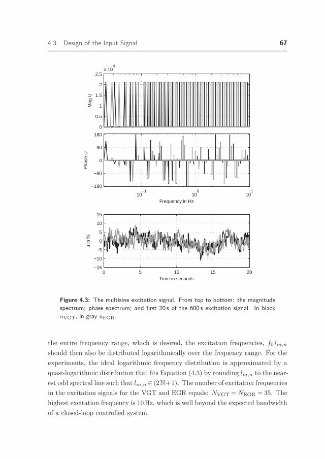
4.3. Design of the Input Signal 67
0
0.5
1
1.5
2
2.5x 10
4
Mag
U
10−1
100
101
−180
−90
0
90
180
Frequency in Hz
Pha
se U
0 5 10 15 20−15
−10
−5
0
5
10
15
Time in seconds
u in
%
Figure 4.3: The multisine excitation signal. From top to bottom: the magnitudespectrum; phase spectrum; and first 20 s of the 600 s excitation signal. In blackuVGT, in gray uEGR.
the entire frequency range, which is desired, the excitation frequencies, f0 lm,n
should then also be distributed logarithmically over the frequency range. For theexperiments, the ideal logarithmic frequency distribution is approximated by aquasi-logarithmic distribution that fits Equation (4.3) by rounding lm,n to the near-est odd spectral line such that lm,n ∈ (2N+1). The number of excitation frequenciesin the excitation signals for the VGT and EGR equals: NVGT =NEGR = 35. Thehighest excitation frequency is 10Hz, which is well beyond the expected bandwidthof a closed-loop controlled system.

68 Chapter 4. Modeling, Identification and Analysis
Particularly at frequencies over 1Hz, the logarithmic distribution of excitationfrequencies on the linear frequency grid of the Discrete Fourier Transform (DFT) isvery sparse. For identification of nonlinear effects, a more dense linear distributionis preferred over the sparse logarithmic distribution (Vanhoenacker et al., 2001).However, for our purposes, an accurate detection of the low frequency linearbehavior has a higher priority than an accurate detection of the high frequencynonlinear behavior. Therefore, the logarithmic distribution is preferred.
To separate the response due to excitation of the EGR valve from the responsedue to excitation of the VGT actuator, two non-overlapping grids of spectral lines,lm,n, are used for the inputs. This enables a separation of the linear effects ofthe individual inputs in the frequency domain and only one experiment is neededto identify the Multi-Input Multi-Output (MIMO) system. In Dobrowiecki andSchoukens (2007), it is shown that the level of nonlinear distortions for MIMOFRF measurements using non-overlapping frequency grids is similar to that of anoptimized experiment using multiple experiments.
Excitation Amplitude
The amplitude Am,n of the individual sinusoids is chosen such that the amplitudeof the combined multisine signal, u[k]
m (t), is similar to the expected amplitude ofthe input signal when a feedback controller for EGR and VGT is active. In thisway, the nonlinear effects that arise during identification are similar to those thatare present during feedback operation. This consideration resulted in a constantamplitude of Am,n = 0.7% of the maximum actuator position for both inputs andall excited frequencies.
4.3.2 Influence of Input Quantization
The amplitude of the individual sinusoids is chosen Am,n = 0.7%, whereas thequantization in the VGT actuator allows only steps of 0.5%. Consequently, thevalues in the smooth multisine signal are rounded towards the nearest integermultiple of 0.5%. Therefore, concerns arise regarding the smoothness and accuracyof the quantized signal that excites the VGT actuator.
To evaluate the influence of quantization of the VGT input, a smooth multisinesignal is compared with a simulated quantized multisine signal. The relative power
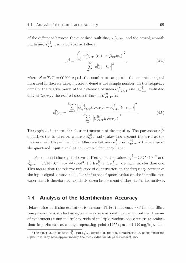
4.4. Analysis of the Identification Accuracy 69
of the difference between the quantized multisine, u[k]q,VGT, and the actual, smooth
multisine, u[k]VGT, is calculated as follows:
e[k]q =
N∑n=1
∣∣∣u[k]q,VGT(tn)−u[k]
VGT(tn)∣∣∣2
N∑n=1
∣∣∣u[k]VGT(tn)
∣∣∣2 , (4.4)
where N = T/Ts = 60000 equals the number of samples in the excitation signal,measured in discrete time, tn, and n denotes the sample number. In the frequencydomain, the relative power of the difference between U [k]
q,VGT and U [k]VGT, evaluated
only at lVGT,n, the excited spectral lines in U [k]VGT, is:
e[k]q,exc =
NVGT∑n=1
∣∣∣U [k]q,VGT(lVGT,n)−U [k]
VGT(lVGT,n)∣∣∣2
NVGT∑n=1
∣∣∣U [k]VGT(lVGT,n)
∣∣∣2 . (4.5)
The capital U denotes the Fourier transform of the input u. The parameter e[k]q
quantifies the total error, whereas e[k]q,exc only takes into account the error at the
measurement frequencies. The difference between e[k]q and e[k]
q,exc is the energy ofthe quantized input signal at non-excited frequency lines.
For the multisine signal shown in Figure 4.3, the values e[1]q = 2.425 ·10−3 and
e[1]q,exc = 6.316 ·10−6 are obtained3. Both e[1]
q and e[1]q,exc are much smaller than one.
This means that the relative influence of quantization on the frequency content ofthe input signal is very small. The influence of quantization on the identificationexperiment is therefore not explicitly taken into account during the further analysis.
4.4 Analysis of the Identification AccuracyBefore using multisine excitation to measure FRFs, the accuracy of the identifica-tion procedure is studied using a more extensive identification procedure. A seriesof experiments using multiple periods of multiple random-phase multisine realiza-tions is performed at a single operating point (1455 rpm and 120mg/inj). The
3The exact values of both e[k]q and e[k]
q,exc depend on the phase realization, k, of the multisinesignal, but they have approximately the same value for all phase realizations.

70 Chapter 4. Modeling, Identification and Analysis
Realization,K
Tt
k = 1
k = 2
k = 3
k = 4
k = 5
k = 6
transientPeriod, J
j = 1 j = 2 j = 3 j = 4 j = 5 j = 6
T T T TT T
Figure 4.4: Scheme of the analysis experiment. For every phase realization k of themultisine signal, J = 6 periods are measured and a total of K = 6 different phaserealizations of the multisine signal are used. Before measuring the periodic response,a waiting time of Tt is introduced to prevent startup transients from disturbing theperiodic measurement (Schoukens et al., 2005).
extended procedure is constructed to analyze the effects of noise and nonlinearitieson the FRF estimate. The analysis also separates nonlinear behavior from thelinear behavior; the nonlinear part is then quantified and classified into even andodd nonlinear behavior. This analysis is performed in the frequency domain and isto a large extent similar to Rijlaarsdam et al. (2010), where the nonlinear behaviorof a single-input industrial motion stage is studied. This section also includes avalidation in the time domain, to further illustrate the model accuracy.
For the purpose of this identification and analysis, the MIMO system canbe split into three separate Multi-Input Single-Output (MISO) systems. Thecalculations and also the analysis are performed for each output separately. Tokeep the notation as short as possible, subscripts to denote the individual outputsare omitted.
To help illustrate the method, Figure 4.4 schematically depicts the executionof the experiment. For each phase realization, k, a multisine input signal u[k] isapplied to the inputs, while the output is measured for J consecutive periods. Inthis chapter, K = 6 phase realizations of the multisine are applied for J = 6 periodseach. In this way, a total of J ·K = 36 periods of measurement data is obtained.Before measuring the periodic response, a waiting time of at least Tt = 60 s is usedfor a sufficient decay of startup transients. The measurement corresponding to asingle period j of realization k is denoted y[k]
j . The length of y[k]j equals one period
of the excitation signal, T = 600 s, and it contains N = 60000 samples. Capital

4.4. Analysis of the Identification Accuracy 71
U and Y , are used to denote the DFT of respectively the inputs u and measuredoutputs y. Measuring multiple periods using the same excitation signal makesit possible to determine the influence of noise. Using multiple realizations of theinput signal makes it possible to determine the influence of nonlinearities on theidentified FRF.
4.4.1 Frequency Response Function
Using the DFT of the applied periodic inputs and measured outputs, the FRF canbe calculated using a division of the transformed signals. The estimated FRF isdefined only at the Nm frequencies present in the input signal: f0 lm,n.
For each input m, period j and realization k, the FRF is calculated as follows:
H[k]j,m(lm,n) =
Y[k]j (lm,n)
U[k]m (lm,n)
. (4.6)
Using all periods of realization k, an average FRF is determined for eachrealization:
H[k]m (lm,n) = 1
J
J∑j=1
H[k]j,m(lm,n). (4.7)
The use of multiple periods reduces the influence of noise on the FRF estimate.The variance of H [k]
m due to noise is a factor J lower than the variance of theindividual estimates H [k]
j,m.
When all realizations of the multisine are used, the FRF estimate can beimproved further:
HBLA,m(lm,n) = 1K
K∑k=1
H[k]m (lm,n), (4.8)
where HBLA,m gives the Best Linear Approximation (BLA) (Schoukens et al., 2005)using the available data. The variance of HBLA,m due to nonlinearities is a factorK smaller than that of the single realization estimates H [k]
m . Also the variancedue to noise decreases by a factor K. For an infinite number of random phaserealizations, HBLA,m converges to the actual best linear approximation, whichdepends only on the power spectrum of the excitation signal.

72 Chapter 4. Modeling, Identification and Analysis
4.4.2 Accuracy of the Frequency Response Function
To analyze the accuracy of the FRF of a single period, H [k]j,m, two sources of
distortion are separated: noise and nonlinearities.
First, the variance due to noise is quantified. Noise causes a repeated exper-iment with the same input signal to have a different outcome. To estimate theexpected distortion of H [k]
j,m due to noise, the variance of the FRF is calculated foreach realization. Next, these variances are averaged over all realizations:
vH,noise,m = 1K (J −1)
K∑k=1
J∑j=1
∣∣∣H [k]j,m− H
[k]m
∣∣∣2 . (4.9)
The distortion due to nonlinear behavior is the same for all periods of thesame realization, but changes when a different phase realization of the input signalis used. The variance of H [k]
m therefore quantifies the expected distortion of H [k]j,m
due to nonlinear behavior:
vH,NL,m = 1K−1
K∑k=1
∣∣∣H [k]m −HBLA,m
∣∣∣2− 1JvH,noise,m, (4.10)
where a correction for the expected bias due to noise is used. Figure 4.5 shows∣∣HBLA,m∣∣ and the standard deviations σH,noise,m = √vH,noise,m and σH,NL,m =
√vH,NL,m for the studied outputs.
The variances calculated in Equations (4.9) and (4.10) are the variances ofH
[k]j,m. The variances of HBLA,m and H [k]
m are lower and can be deduced by dividingby J and K, according to the methods provided in Section 4.4.1.
Figure 4.5 shows that the expected deviation of the FRF due to nonlinearitiesdominates over the expected deviation due to noise. Where
∣∣HBLA,m∣∣ is an order
of magnitude larger than the deviation due to either noise or nonlinearities, H [k]j,m
is considered an accurate estimate of HBLA,m. Which implies that an FRF thatis made using a single period of ten minutes is an accurate estimate of the actualBLA. The values of
∣∣HBLA,VGT∣∣ are larger than those of
∣∣HBLA,EGR∣∣, whereas
their respective standard deviations have similar values. This means that therelative accuracy of
∣∣HBLA,VGT∣∣ is higher. Nonlinear distortions are the largest
cause of variance. Therefore, increasing the number of periods, J , is much less

4.4. Analysis of the Identification Accuracy 73
10−5
10−4
10−3
10−2
10−1
100
NO
x
VGTEGR
10−6
10−5
10−4
10−3
10−2
10−1
λ
10−1
100
101
10−4
10−3
10−2
10−1
100
101
∆p
Frequency in Hz
Figure 4.5: Analysis of the variance of H [k]j,m for the operating point 1455RPM
and 120mg/inj. The response of the VGT and EGR inputs is depicted in respectivelyblack and gray. The lines show
∣∣HBLA,m∣∣; the ’x’ and ’o’ symbols show respectively
σH,noise,m and σH,NL,m.
effective at improving the accuracy of HBLA,m than increasing the number ofrealizations, K.
Particularly for the ∆p output, the variances due to noise and nonlinearitiesare very low, i.e., HBLA,m is very accurate for the ∆p output. This is also reflectedin the smoothness of
∣∣HBLA,m∣∣ for the ∆p output.
The measurement of∣∣HBLA,m
∣∣ for the NOx output is, at the anti-resonance

74 Chapter 4. Modeling, Identification and Analysis
around 0.6Hz, of the same magnitude as σH,NL,m. A single measurement ofH
[k]j,m will, therefore, not suffice to reliably determine HBLA,m for this frequency.
However, the presence of the anti-resonance can be determined reliably from asingle measurement, because σH,NL,m is significantly smaller than the FRF valuessurrounding the anti-resonance.
4.4.3 Classification of Nonlinearities
The previous section dealt with determining how accurate the BLA of the FRF isdetermined. This section deals with determining how accurate this BLA describesthe actual system behavior. Opposed to the FRF models discussed in the previoussection, which only describe the linear behavior of the system, this section focusseson quantifying and classifying the remaining nonlinear part of the system. Ananalysis of the measured outputs at non-excited spectral lines reveals the quantityof the output power omitted from the linear model.
The response of a linear system that is excited with a periodic input signal isagain a periodic signal containing only the frequencies present in the input signal.The response of a nonlinear system includes frequencies that are not present in theinput signal. By analyzing the spectral content of the measured data at non-excitedfrequencies, the nonlinear behavior can be analyzed. The nonlinear part of theresponse can be classified into an even and an odd part. The frequency content ofthe higher-order harmonics generated by the even part of the nonlinear behaviorconsists of even multiples of the excitation frequencies and vice versa for the oddpart.
The input signals u[k]m consist of only odd frequencies (odd multiples of f0).
Odd multiples of odd frequencies result again in odd frequencies. Even multiples ofthe odd frequencies in the excitation signal result in even frequencies. Therefore, aseparation of the spectrum of y[k] into even and odd multiples of the base frequencyseparates of the effects of even and odd nonlinear behavior.
The average DFT of the output spectrum of a single realization is given by:
Y [k] = 1J
J∑j=1
Y[k]j (4.11)

4.4. Analysis of the Identification Accuracy 75
and the variance of Y [k] due to noise is given by:
v[k]Y,noise = 1
J (J −1)
J∑j=1
∣∣∣Y [k]j − Y
[k]∣∣∣2 . (4.12)
Using Y [k] and v[k]Y,noise, the power in the output spectrum due to nonlinearities,
corrected for the expected bias due to noise, is:
PNL = 1K
K∑k=1
∣∣∣Y [k]∣∣∣2− 1
K
K∑k=1
v[k]Y,noise. (4.13)
To make the results of (4.13) of the same units as the FRF (HBLA,m) andthereby easier to interpret, the square root of the power is calculated and scaledwith the magnitude of the input signal. This results in DNL:
DNL =√PNL
U(4.14)
and for the estimated noise bias of DNL:
Dnoise =
√1K
K∑k=1
v[k]Y,noise
U, (4.15)
where U =∣∣∣U [k]j,m (lm)
∣∣∣ = 12N ·Am,n is used to scale the results with the input
amplitude. A constant amplitude is used for both inputs at all excited frequencies,therefore U is also constant, as can be observed in Figure 4.3.
To separate the even and odd nonlinear behavior, the data of DNL in (4.14) issplit into two different frequency ranges, which separate the odd frequencies (lo ∈Lo = {l ∈ 2N+ 1 | l 6= lm,n ∀m,n}) from the even frequencies(le ∈ Le = (2N+ 2)) .
Figure 4.6 shows a comparison between∣∣HBLA,m
∣∣, DNL(le), DNL(lo) andDnoise. At high frequencies Dnoise is of similar magnitude as DNL, which indicatesthat the values for DNL are unreliable. Except for the anti-resonance in theNOx-output and the frequency range around 10Hz, the nonlinear part of thesystem behavior, DNL, is an order of magnitude smaller than the linear behavior,∣∣HBLA,m
∣∣. This means that a linear FRF relevantly describes the actual dynamicsystem behavior. This result extends beyond multisine identification; it implies

76 Chapter 4. Modeling, Identification and Analysis
10−5
10−4
10−3
10−2
10−1
100
NO
x
10−6
10−5
10−4
10−3
10−2
10−1
λ
10−1
100
101
10−4
10−3
10−2
10−1
100
101
Frequency in Hz
∆p
Figure 4.6: Frequency content of the non-excited spectral lines. The engine oper-ating point is 1455RPM and 120mg/inj. The black and gray line show respectively∣∣HBLA,VGT
∣∣ and ∣∣HBLA,EGR∣∣. The medium gray, light gray and dark gray dots
show respectively Dnoise, DNL(le) and DNL(lo).
that when the input signals are similar to those during the identification, lineartechniques are relevant for analysis of the dynamics and linear control theory issuitable for the design of local controllers.
Particularly for ∆p a difference between odd and even nonlinearities is ob-served. At low frequencies, the effect of the even nonlinearities is an order ofmagnitude higher. Because only odd frequencies are used for measuring the FRF,
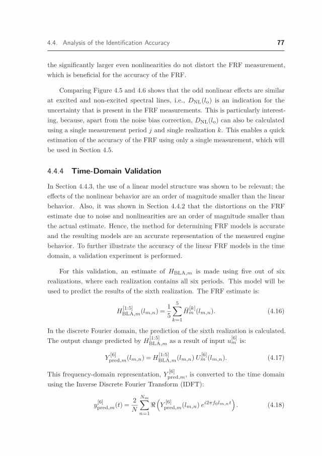
4.4. Analysis of the Identification Accuracy 77
the significantly larger even nonlinearities do not distort the FRF measurement,which is beneficial for the accuracy of the FRF.
Comparing Figure 4.5 and 4.6 shows that the odd nonlinear effects are similarat excited and non-excited spectral lines, i.e., DNL(lo) is an indication for theuncertainty that is present in the FRF measurements. This is particularly interest-ing, because, apart from the noise bias correction, DNL(lo) can also be calculatedusing a single measurement period j and single realization k. This enables a quickestimation of the accuracy of the FRF using only a single measurement, which willbe used in Section 4.5.
4.4.4 Time-Domain Validation
In Section 4.4.3, the use of a linear model structure was shown to be relevant; theeffects of the nonlinear behavior are an order of magnitude smaller than the linearbehavior. Also, it was shown in Section 4.4.2 that the distortions on the FRFestimate due to noise and nonlinearities are an order of magnitude smaller thanthe actual estimate. Hence, the method for determining FRF models is accurateand the resulting models are an accurate representation of the measured enginebehavior. To further illustrate the accuracy of the linear FRF models in the timedomain, a validation experiment is performed.
For this validation, an estimate of HBLA,m is made using five out of sixrealizations, where each realization contains all six periods. This model will beused to predict the results of the sixth realization. The FRF estimate is:
H[1:5]BLA,m(lm,n) = 1
5
5∑k=1
H[k]m (lm,n). (4.16)
In the discrete Fourier domain, the prediction of the sixth realization is calculated.The output change predicted by H [1:5]
BLA,m as a result of input u[6]m is:
Y[6]pred,m(lm,n) =H
[1:5]BLA,m(lm,n) U [6]
m (lm,n). (4.17)
This frequency-domain representation, Y [6]pred,m, is converted to the time domain
using the Inverse Discrete Fourier Transform (IDFT):
y[6]pred,m(t) = 2
N
Nm∑n=1<(Y
[6]pred,m(lm,n) ei2πf0lm,nt
). (4.18)

78 Chapter 4. Modeling, Identification and Analysis
The nominal static output is not predicted by the FRF measurements. The averageoutput over the first five realizations is used instead:
y[1:5]s = 1
5N
5∑k=1
N∑n=1
y[k](tn). (4.19)
Using the superposition principle, the sum of y[1:5]s and y[6]
pred,m evaluated for boththe VGT and EGR produces the prediction of y[6]:
y[6]pred(t) = y
[1:5]s +y
[6]pred,VGT +y
[6]pred,EGR. (4.20)
Figure 4.7 shows a comparison between y[6]pred(t) and the measured output
of the sixth realization averaged over all periods: y[6](t) = 1J
∑Jj=1 y
[6]j (t). As
expected from the earlier frequency domain results, a close match between themodel prediction and measured output is observed.
Various aspects of the accuracy of the model fit are quantified. The totalrelative error is calculated using:
etotal =
N∑n=1
(y
[6]pred(tn)−y[1:5]
s − y[6](tn) + y[6]s)2
N∑n=1
(y[6](tn)− y[6]
s)2
, (4.21)
where y[6]s = 1
N
∑Nn=1 y
[6] (tn). A correction for the static values is used, such thatetotal quantifies only errors in the dynamic behavior; the prediction of the staticoutput is not of interest for FRF modeling.
The fraction of the power of the measurement signal at frequencies that arenot present in the excitation signal is given by:
eo/e =
No/e∑n=1
∣∣∣Y [6](lo/e,n)∣∣∣2
N∑l=1
∣∣Y [6](l)∣∣2 , (4.22)
with lo/e ∈ (Lo ∪Le), the non-excited spectral lines and No/e = N/2− (NVGT +NEGR), the number of non-excited spectral lines. The error eo/e indicates therelative influence of nonlinear behavior.
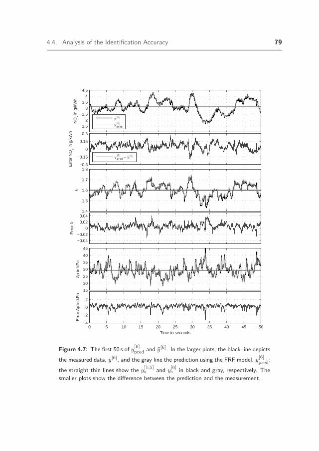
4.4. Analysis of the Identification Accuracy 79
1.52
2.53
3.54
4.5
NO
x in g
/kW
h
y [6]
y[6]pred
1.4
1.5
1.6
1.7
1.8
λ
15
20
25
30
35
40
45
∆p in
kP
a
−0.3
−0.15
0
0.15
0.3
Err
or N
Ox in
g/k
Wh
y[6]pred− y [6]
−0.04
−0.02
0
0.02
0.04
Err
or λ
0 5 10 15 20 25 30 35 40 45 50−4
−2
0
2
Err
or ∆
p in
kP
a
Time in seconds
Figure 4.7: The first 50 s of y[6]pred and y[6]. In the larger plots, the black line depicts
the measured data, y[6], and the gray line the prediction using the FRF model, y[6]pred;
the straight thin lines show the y[1:5]s and y[6]
s in black and gray, respectively. Thesmaller plots show the difference between the prediction and the measurement.

80 Chapter 4. Modeling, Identification and Analysis
The relative error at the frequencies present in input signal m equals:
em =
Nm∑n=1
∣∣∣Y [6]pred,m(lm,n)− Y [6](lm,n)
∣∣∣2Nm∑n=1
∣∣Y [6](lm,n)∣∣2 (4.23)
and for both inputs combined:
eexc =
∑m∈{VGT,EGR}
Nm∑n=1
∣∣∣Y [6]pred,m(lm,n)− Y [6](lm,n)
∣∣∣2∑
m∈{VGT,EGR}
Nm∑n=1
∣∣Y [6](lm,n)∣∣2 . (4.24)
The values em and eexc quantify the error that is made in predicting the linearbehavior of the engine.
In Table 4.1, an overview of the differences between the measurement y[6] andmodel prediction y[6]
pred is presented. Note that none of the error measures use abias correction for noise or nonlinearities. Therefore, when a different number ofperiods or realizations is used, the expected values of these error measures changes.Figures 4.5 and 4.6 and Equations (4.9), (4.10), (4.14) and (4.15) provide lessambiguous error measures in this sense. The comparison also differs from thecomparison in Figures 4.5 and 4.6, it is not aimed at determining the accuracy ofan FRF model made using a single measurement period. Instead, the predictionof an average FRF model is compared with the expected value of a single experi-ment. In this comparison nonlinear effects are present mostly in the measurement.Because multiple realizations are used for determining y[6]
pred,m, nonlinear effectsare averaged in the prediction. Noise has a very small effect on the accuracy ofy
[6]pred,m and averaging of six periods is used to decrease the effects of noise fromthe measurement.
The relative power of the error is at most 2.8 percent for all outputs. Surpris-ingly, the NOx measurement is predicted more accurately than the ∆p measure-ment, even though the relative variance of the FRF was significantly smaller for∆p. When looking at eexc it can be seen that indeed the linear part of the ∆presponse is recreated with the highest accuracy, but nonlinear effects are the main

4.4. Analysis of the Identification Accuracy 81
Table 4.1: The relative difference between model and measurement.
etotal eo/e eexc eVGT eEGR
NOx 1.41% 1.23% 0.18% 0.11% 0.70%
λ 2.80% 2.55% 0.26% 0.15% 0.89%
∆p 1.64% 1.61% 0.03% 0.02% 0.07%
cause of etotal. The even nonlinear behavior observed in the ∆p measurement didnot disturb the FRF measurement, but does show up in eo/e. When only eexc,eVGT and eEGR are considered, which only quantify errors in the linear part ofthe response, the ∆p prediction is the most accurate.
For all outputs, eo/e constitutes the largest part of etotal. Only nonlinearmodels can capture these effects. To significantly decrease the remaining error, anonlinear model is needed.
The errors in Table 4.1 might be surprisingly small, but two remarks are inplace here. First, the relative power of the error is considered. This means thatcompared to Figures 4.5 and 4.6, the relative difference is squared. Second, theparts of the FRF with high gains are identified most accurately. These parts alsoconstitute a relatively large part of the power of the output signal. This also favorslow errors in the time-domain validation compared with the frequency-domainresults in Figures 4.5 and 4.6.
In the presented form, the FRF models are not directly suitable for simu-lating the response to a general input signal that includes different frequencies.Approximations are needed to enable a calculation of the response at frequenciesthat are not present in the excitation signal. Furthermore, it is known that theBLA depends on the power spectrum of the input. For inputs with smaller orlarger amplitudes, the BLA will change. Using common knowledge of the nonlin-ear behavior of the air path, it is expected that the accuracy will degrade whenlarger input amplitudes are considered, because nonlinear effects will constitute alarger part of the output spectrum. When the input amplitude is decreased, therelative influence of noise and quantization will increase, but the nonlinear effectsare expected to decrease. As noise and quantization currently constitute a minoreffect, the approximation error is expected to decrease when the input amplitude
82 Chapter 4. Modeling, Identification and Analysis
is decreased. For the presented identification results, the input amplitude waschosen to make the input signal resemble the output of a feedback controller. Thismakes the identification results and accuracy analysis particularly suited towardsfeedback control design.
4.5 Frequency Response Function MeasurementResults
From Section 4.4, it is concluded that the standard deviation of the resulting FRFmeasurements is an order of magnitude smaller than the actual FRF itself, evenwhen a single measurement period is used. When the conclusion of this analysisholds for all operating points, the FRF at a different operating point can be identi-fied efficiently using a single 600 s period. To check this assumption, the accuracy ofthe FRF and encountered nonlinearities can be determined using Equation (4.14).The bias estimate cannot be included, because only one measurement period isavailable.
To characterize the differences in the input-output behavior of the diesel engineat different operating points, FRF measurements on a 3x3 grid of engine speeds(1011, 1455, 1700 rpm) and loads (60, 120, 200 mg/inj) are performed. Ten minutesof measurement time is used for each operating point and the FRF is calculatedusing Equation (4.6). Figure 4.8 shows the resulting FRFs in a Bode plot. UsingEquation (4.14), it is concluded that the ratio between the linear and nonlinearcontributions is similar to Figure 4.6, which implies that indeed the analysis ofSection 4.4 will render similar results for all operating points.
Some salient features of the dynamic behavior of the engine in the differentoperating points are observed in Figure 4.8. The gain differences between differentoperating points are of a full order of magnitude and are present for all input andoutput combinations. On the other hand, the variations in phase between thedifferent operating points are remarkably small; apart from some large variationswhich are discussed separately.
The FRFs of the VGT are of similar magnitude as the FRFs of the EGR forall outputs. This means that coupling is present between all inputs and outputs.
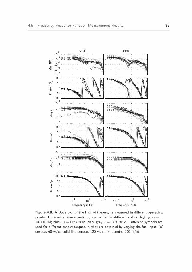
4.5. Frequency Response Function Measurement Results 83
10−4
10−3
10−2
10−1
100 VGT
Mag
NO
x
−180
−90
0
90
180
Pha
se N
Ox
EGR
10−4
10−3
10−2
10−1
Mag
λ
−180
−90
0
90
180
Pha
se λ
10−2
10−1
100
101
Mag
∆p
10−1
100
101
−180
−90
0
90
180
Pha
se ∆
p
Frequency in Hz10
−110
010
1
Frequency in Hz
Figure 4.8: A Bode plot of the FRF of the engine measured in different operatingpoints. Different engine speeds, ω, are plotted in different colors: light gray ω =1011RPM; black ω = 1455RPM; dark gray ω = 1700RPM. Different symbols areused for different output torques, τ , that are obtained by varying the fuel input: ’o’denotes 60mg/inj; solid line denotes 120mg/inj; ’x’ denotes 200mg/inj.

84 Chapter 4. Modeling, Identification and Analysis
For control design this means that MIMO design techniques are required to obtainthe best performance.
In the phase plot of the VGT-λ FRF, a low frequency sign change is observed at1700 rpm and 200 mg/inj. This potentially induces difficulties for feedback controldesign. In Wahlström (2009), the gain differences, coupling and sign changes arealso observed, using a mean-value model of a different engine with a similar layout.
The anti-resonance found in the EGR-NOx FRF changes between minimumand non-minimum phase. A closer analysis of the individual sensor data of theNOx sensor and air-flow sensor explains this behavior and has shown that thisanti-resonance is caused by the interaction of different sensor dynamics and is nota physical property of the engine dynamics.
The FRF measurements indicate that sensor dynamics form a significant partof the dynamic input-output behavior. In the phase plots in Figure 4.8, the delay inthe response of the system can be observed. In particular for the NOx measurement,delay has a significant influence on the phase of the FRF. For frequencies over 0.3Hz,the phase lag due to delay largely determines the phase of the FRF. Moreover, theobserved time scales are different for each output, which could also be observedin Figure 4.7. The NOx response contains less power at high frequencies (over1Hz) than the ∆p response. Both the delay and observed difference in time scalesindicate the influence of sensor dynamics.
It should be noted that the results on the 3x3 speed-load grid are only intendedto assess the global properties of the engine in a qualitative manner. Only at theselected operating points, the accuracy is comparable with the results of Table 4.1.To model the engine behavior in between the grid points, interpolation can beused, but the prediction accuracy will depend much more on the nonlinearity ofthe engine behavior than on the accuracy with which the local behavior at the gridpoints was captured.
For control applications, a different grid can be selected. The most suitablegrid size depends on the type of controller. Some examples are found in literature:the controller in Ortner and Del Re (2007) uses 12 grid points and Ferreau et al.(2007) uses only two grid points. In Henningsson et al. (2012), the engine behavioris modeled only at 1200RPM and up to mid-load. It is shown that when 4 or 6 gridpoints in this small range are selected, 10% or 5% accuracy is lost, respectively.

4.6. Discussion 85
4.6 Discussion
The presented non-parametric modeling approach shows a high accuracy and isefficient in terms of the required measurement time, when applied to the dieselengine air path. The intended use of the FRF models is air-path feedback controldesign. For this purpose, the dynamic input-output response around an operatingpoint is important. Feed-forward controllers, that bring the engine operatingconditions close to the nominal conditions, are assumed to be present in theengine control system. In this case, the identified local models provide a relevantdescription of the dynamic behavior. Under these conditions, the identificationaccuracy is very high. From the results in Table 4.1, it can be deduced that theVariance Accounted For (VAF) is at least 97.2% for the considered outputs. Thisvalue can be compared with alternatives found in the literature. In Henningssonet al. (2012), a VAF between 64.3% and 93.5% is obtained. The LPV modelused in Wei and Del Re (2007) obtains a VAF of 85%. The achieved accuracywith the proposed modeling approach exceeds the accuracy of alternative methods.However, for applications other than control design and analysis, the usability ofthe presented FRF models is limited.
The identification accuracy, as shown in this chapter, largely depends on thelinearity of the input-output response. Although the local behavior (i.e. the behav-ior around a fixed state) of a nonlinear system is often close to linear, this it is notnecessarily true for a relevant input range. This dependency gives rise to a concernwhen different inputs or outputs are selected. Moreover, when different outputsare chosen, the noise characteristics will differ, which influences the identificationaccuracy. This is why it is critical that the model accuracy can be quantified, as isdone is Section 4.4, and it is revealed to what extent the identified linear systemdescription is accurate.
For accurately modeling or simulating large operating-point variations, or formodeling input variations spanning the full actuator range, the presented method-ology is not well-suited. It can be expected that the analysis for nonlinearities willshow that linear models no longer relevantly describe the engine behavior and themodel quality will degrade. In Figure 4.7, it can be observed that the model accu-racy decreases at output peaks. Modeling the engine behavior for conditions thatsignificantly deviate from nominal is outside the scope of this article. Models that

86 Chapter 4. Modeling, Identification and Analysis
describe this behavior accurately have to be nonlinear, e.g., mean-value models aremuch more valuable for this.
Despite these disadvantages, the FRF models have numerous advantages re-lated to control design. The FRF representation used in this article is suitableto describe systems for which linear dynamics are dominant and is fit to workwith broadband multisine identification. Also, classical (PID) controllers can bedesigned directly in the frequency domain using FRF models, which is done forair-path control in Criens et al. (2014). Moreover, the FRF models can providestrong analysis results, e.g., for decoupling control design or can be used to ana-lyze the dynamic properties achieved with various controllers. For simulation orintegration with model-based control synthesis, e.g., Linear Quadratic Gaussian(LQG) optimal control or MPC, a state-space or transfer-function representationis necessary. Software tools are available to convert the measurement data into atransfer function. The n4sid algorithm of the System Identification Toolbox inMATLABR©, as applied in Henningsson et al. (2012), can be used for this. TheBLA can be approximated with arbitrary accuracy by increasing the approximationorder. Depending on the application, a suitable system order should be selected.In Henningsson et al. (2012), a model order of 7 is proposed and it is shown thatmodel orders below 5 lead to a poor prediction, whereas in Wei and Del Re (2007)a model of order 3 is used to facilitate quasi-LPV control design.
4.7 Conclusions
Multisine identification is successfully used as an efficient method for determiningthe local dynamic behavior of a diesel engine air path, using the VGT and EGRvalve as inputs. An accurate non-parametric model of the linear MIMO behavior ofthe engine, in the form of an FRF, is identified using ten minutes of measurementdata. The FRF provides a control-relevant description of the local input-outputbehavior at a single operating point, naturally including sensor and actuatordynamics. The considered outputs are NOx, air-fuel equivalence ratio and pressuredifference between intake and exhaust manifold. In particular NOx emissions aredifficult to model using first-principles models, but straightforward to include usingFRFs.

4.7. Conclusions 87
Quantifying the influences of noise and nonlinearities on the FRF measurementis an essential part of the presented identification method. The nonlinear part ofthe engine behavior is quantified and classified and the ability of linear models todescribe the encountered behavior is quantified. It was discovered that the influenceof nonlinear behavior is an order of magnitude smaller than the magnitude of thelinear behavior. This means that linear dynamics largely determine the local enginebehavior and linear techniques are relevant for system analysis and control design.It is shown that, using a linear FRF model, validation data can be reproducedwith errors below 2.8%. The remaining error is largely caused by the lack of adescription of the nonlinear behavior.
To characterize the global behavior of the engine, multisine identification wasused to identify FRFs for a range of engine operating points. The behavior variessignificantly as a function of the operating point: gain differences of a full orderof magnitude, sign changes and large phase variations are captured using FRFidentification.


5 Control for DisturbanceRejection, Low Emissions andHigh Fuel Efficiency
89
5.1 IntroductionWith the recent introduction of EURO VI, not-to-exceed and on-road emissionlimits are introduced. These limits restrict the exhaust emissions of diesel enginesunder diverse and uncertain conditions. The WNTE and in-service emissions areaffected by the uncertain drive cycle. The in-service emissions are also affected byexternal factors, e.g., ambient temperature, ambient pressure, humidity and fuelquality, and also internal factors, e.g., ageing, engine wear, production tolerances,engine temperature and actuator hysteresis. These uncertain factors make themeasured emissions over these two tests less predictable and reproducible.
To comply with the new legislation, despite the uncertain factors, two ap-proaches are possible. Either, additional margins between the nominal exhaustemissions and the legislation limits are introduced, such that the worst case sce-nario still complies with the emission legislation. Or, adaptations of the enginesettings should be made, such that the engine adapts to the unknown conditionsto ensure that the exhaust emissions always remain close to the nominal levelsthat are known to comply with legislation. The former option may seem beneficialfor the environment, because the nominal pollutant emissions are reduced. But,as a result of the tradeoff between emissions and fuel efficiency, a fuel penalty isinvolved with reducing the engine-out emissions. This increases the operationalcosts and the increased CO2 emissions and use of hydrocarbons have a negativeenvironmental effect. Moreover, the emission limits set in EURO VI require drasticreductions of the tailpipe NOx and PM exhaust emissions, compared with EUROV and are very challenging. This makes reducing the emissions beyond these limits

90 Chapter 5. Feedback Control for Disturbance Rejection
practically unacceptable. Consequently, a control strategy is needed to ensurethat the achieved exhaust emissions remain close to the nominal exhaust emissionsdespite the influences of uncertain factors.
In this chapter, the design of an air-path control system for disturbance rejec-tion in diesel engines is elaborated. First, the control problem is described in moredetail. Next, a conceptual control design for disturbance rejection is presented andtested in simulation. Based on this conceptual design, but adapted for the currentengine hardware, a second controller is designed. This controller is implemented onprototype control hardware and experimentally tested and evaluated on a modernengine.
5.2 Control Problem
The high-level goals of the engine control system in a heavy-duty diesel engine areto provide the requested amount of torque with minimum fuel consumption, whilecomplying with emission legislation and remaining within safety and durabilitylimits.
In this chapter, only disturbance compensation is considered. It is assumedthat the operating point is quasi-stationary, such that all control aspects related tospeed and load dynamics can be disregarded. Second, optimal input setting thatachieve the above high-level control goal at the current stationary operating pointunder nominal conditions are assumed to be a priori available. When the enginebehavior or the external conditions deviate from nominal, the nominal, optimalinput settings should be adapted to maintain optimal performance. The aim ofthis chapter is to design a control algorithm that achieves this.
To minimize the fuel consumption within the emission constraints defined inlegislation, a complex tradeoff between the allowed engine-out emissions and fuelefficiency is made. The emissions and fuel efficiency vary over the engine speedand load range, such that the expected in-service fuel consumption is minimized.When the nominal actuator settings are used as determined during calibration,while disturbances are present, the engine-out emissions and fuel consumption will

5.2. Control Problem 91
deviate. Unless the aftertreatment system is able to counterbalance this, compli-ance with legislation is no longer guaranteed. Also, an increased fuel consumptionmight be observed. In consequence, the high-level goals are no longer achieved.
In this chapter, a controller is designed to improve on the above situation.The high-level control goals are, however, not very suitable to be used directlyin a control design. Compliance with emission legislation is determined over acycle and cannot be determined unambiguously from measurements at a singlepoint in time. Similarly, the fuel consumption should be evaluated over a fulland realistic drive cycle, rather than instantaneously. These are unfortunateproperties, as it is difficult to determine whether additional control actions areneeded and also to evaluate if the current emissions and fuel consumption areoptimal. Therefore, rather than aiming directly for minimum fuel consumptionwhile achieving compliance with emission legislation, a goal that is better suitedfor control design is formulated:
Maintain the BSFC, NOx emissions and PM emissions at all times asclose as possible to the values obtained under nominal conditions.
After calibrating the engine, the nominal values for the BSFC, NOx and PMwill be such that a simultaneous reduction of all three aspects is not possible.Any known possibility for reducing all three performance aspects simultaneously,that does not require violating a constraint, will be exploited in the calibrationprocess. The BSFC, NOx and PM after calibration therefore form a Pareto optimalpoint. This implies that functional controllability of these three outputs is notpossible. Moreover, it is likely that the exact same values for BSFC, NOx and PMthat are obtained under nominal conditions are either no longer reachable or nolonger optimal, when disturbances are present. For this reason, rather than aimingfor exact tracking, the goal is to remain as close as possible to the performancemeasures.
Disturbance rejection in this form offers the following three potential advan-tages.
• Reduced variation of the engine-out emissions and fuel consumption. Thisprovides an opportunity to reduce the margins needed to ensure compliancewith the in-service conformity legislation.

92 Chapter 5. Feedback Control for Disturbance Rejection
• Reduced average emissions as a result of preventing excessively high emis-sions. As a result of the exponential increase of NOx with temperature,the increase in NOx due to disturbances will be larger than the decreasein NOx. Consequently, the average NOx will increase due to uncertainties.Similarly, the PM emissions increase rapidly when the air-fuel equivalenceratios approaches unity, whereas they become relatively insensitive to in-creases towards higher air-fuel equivalence ratios. Disturbance rejection cantherefore decrease the average NOx and PM emissions.
• Reduced fuel consumption through improved calibration. As a result of boththe reduced variation of the emissions and the reduced average emissions,the nominal emission levels can be allowed to increase. In consequence ofthe tradeoff between the emissions and fuel consumption, this provides anopportunity to reduce the fuel consumption at the expense of an increase inthe nominal emissions.
The goal of this chapter is to design a controller that combines all threeadvantages.
An important design specification of a feedback control design is the band-width1. To determine an appropriate value, the conditions where the feedbackcontroller is used are analyzed. Several disturbances or uncertainties that poten-tially affect the emissions and fuel consumption are present, when a diesel engineis used in a commercial vehicle. External factors such as the ambient temperature,ambient pressure, humidity and fuel quality, and also internal factors, such as age-ing, engine wear, production tolerances and engine temperature can be considered.A similarity between these disturbances is that the typical time scale on whichthey act is several minutes, hours or more. The target bandwidth for the feedbackcontroller is however much faster than the time scale of the disturbances. Speedand load variations that occur in a typical drive cycle of a diesel engine have to betaken into account. The time scale associated with these speed and load variationsis of the order of several seconds. In a typical control layout, feed-forward controlschemes are used to accommodate these operating point variations. Nonetheless,the feedback controller should readapt the inputs after the operating point has
1In this thesis, bandwidth is defined as the frequency up to which the magnitude of the highestsingular value of the sensitivity is below 0 dB.

5.3. Conceptual Design 93
changed to maintain the desired disturbance rejection. Therefore, a target band-width of 0.2Hz will be used. Results in the literature such as Stewart et al. (2010);Wahlström and Eriksson (2008); Alfieri (2009); Stefanopoulou et al. (2000) indicatethat similar values for the bandwidth are used. A much faster bandwidth willinterfere with the operating point transients; a much slower bandwidth will resultin a poor tracking performance with dynamic drive cycles.
5.3 Conceptual DesignA feedback controller uses sensor measurements, a control algorithm and actuatorsto influence the behavior of the system. For the studied engine control problem,the choice for all three parts is nontrivial. This section motivates the choices forall three parts.
5.3.1 Actuators
The main actuators in a heavy-duty diesel engine that affect the NOx and PMemissions and fuel efficiency are the Variable Geometry Turbine (VGT), ExhaustGas Recirculation (EGR) valve and Start Of Injection (SOI)2. To be the leastconservative and have the best performance potential, generally all three availableactuators should be used in the control design. However, to successfully employan actuator in a feedback controller, sensors are equally important as actuators.For this reason the use of the SOI as an actuator is reconsidered.
The SOI can have a large effect on the engine-out emissions and fuel efficiencyof a diesel engine (Guzzella and Amstutz, 1998; Brahma, 2005). Also, its fast,almost instant, dynamic response makes the SOI convenient for closed-loop control.However, sensors to measure the effects of the SOI are lacking in heavy-dutyproduction engines, which hinders the usability of the SOI in a feedback loop. The
2Other actuators can be considered as well. A variable swirl valve or variable valve actuationcan be available on some engines, but these are not available on the considered engine type. Aback-pressure valve or intake throttle can be used on heavy-duty engines, but because additionalthrottling of the air flow has a detrimental effect on fuel efficiency, they are only used whennecessary and fully opened otherwise. The rail pressure in the fuel path can also be used as anactuator. However, to simultaneously minimize the engine-out NOx and PM emissions, the railpressure is typically set as high as possible. This makes these actuators not very suitable forfeedback control

94 Chapter 5. Feedback Control for Disturbance Rejection
effect of the SOI on the engine-out NOx emissions is measured by means of a NOx
sensor, but sensors to determine the effects of the SOI on the PM emissions andfuel efficiency are not available currently. The use of equipment for measuring PMemissions or smoke (as used in Karlsson et al. (2010) and Tschanz et al. (2013)) islimited to research engines and is not available in production yet. Also, in-cylinderpressure sensors3 (as used in Karlsson et al. (2010) and Zhao et al. (2013)) or torquesensors to measure the effects of the SOI on the fuel efficiency are not available oncurrent heavy-duty production engines. Such sensors would be required to benefitfrom using SOI in a feedback loop. The combustion timing is directly affected bythe SOI and both early and late combustion have a detrimental impact on the fuelefficiency. Moreover, late combustion timing increases the PM emissions. Whenthe SOI is adapted based on the measured NOx emissions only, a simultaneouseffect on the BSFC and PM emissions will be present, but this effect will notbe measured by the engine sensors. Both the BSFC and the PM emissions willincrease, when NOx is reduced via the SOI. Without the proper sensors, it cannotbe determined if the achieved change in NOx outweighs the increase in PM andBSFC. And similarly if this adaptation of the SOI brings the engine performancecloser to a desired situation, when all three performance measures are taken intoconsideration. The SOI is therefore not used as an actuator for feedback control.This reduces the available feedback actuators to the VGT and EGR valve:
ufb =[ufb,VGT ufb,EGR
]ᵀ. (5.1)
Limiting the actuators used for feedback control to the VGT and EGR valvedoes not change that the PM emissions and BSFC cannot be measured directly.However, because the VGT and EGR valve act on the air path, measurementsin the air path can be used to substitute direct PM and torque measurements,which is elaborated in Section 5.3.2. This enables a control design that takes allthree performance aspects into account, despite the shortcomings of the availablesensors. Similar substitutions to measure the effects of the SOI are not available.
3When in-cylinder pressure sensors are available, the control problem changes considerably.These sensors are well suited to be combined in a feedback loop with the actuators in the fuelpath and provide various opportunities for combustion control. This is briefly discussed inSection 7.2.1.2. The difference in time scales that exists between the air path and fuel path likelystill allows for a separate control design, without inducing a significant performance penalty.

5.3. Conceptual Design 95
5.3.2 Controlled Outputs
To make feedback control most effective, the controlled outputs are chosen toreflect the main performance measures: NOx emissions, PM emissions and fuelefficiency, as directly as possible. For each performance measure, a relevant outputis selected.
To quantify the engine-out NOx emissions and PM emissions, direct measure-ments are used in this conceptual design. It is known that the NOx sensor usedon production diesel engines suffers from sensor dynamics, which complicates itsuse in feedback control systems. Moreover, on current production engines, PMmeasurements are not available. For this conceptual design, these shortcomings areoverlooked. The engine-out NOx and PM emissions are assumed to be measuredaccurately and instantaneously.
Taking into account the BSFC is more complex than the emissions. The BSFCat a certain operating point is affected by several factors; the air path, the fuelpath, external disturbances and internal uncertainties all affect the fuel efficiency.It is not desirable that the VGT and EGR valve compensate for all contributingfactors. Consider and example case where the friction losses increase comparedwith the nominal situation. Using the VGT and EGR valve, the friction cannot beinfluenced. But the increased BSFC can be compensated for by increasing the air-fuel ratio, decreasing the EGR flow and decreasing the pumping work. When thesecompensations are applied, the BSFC will decrease, but the in-cylinder conditionswill deviate more from the nominal conditions than when they are not applied.This will compromise the performance elsewhere. It is therefore not an effectivemethod for disturbance rejection; an alternative measure for fuel efficiency shouldbe used.
The air-path affects the BSFC in two ways. First via IMEPg and second viaPMEP. IMEPg is affected by the in-cylinder air mixture. This mixture thoughis largely determined to obtain low engine-out NOx and PM emissions, ratherthan to maximize IMEPg. The NOx and PM emissions are already selected ascontrolled outputs and via control of these emissions the intake mixture will beadapted to have the desired composition with respect to these outputs. Theremaining effect of disturbances in the air path on IMEPg can be expected tobe small and moreover necessary to maintain the emissions at the desired level.

96 Chapter 5. Feedback Control for Disturbance Rejection
Therefore, PMEP is the relevant measure to determine the effect of the air pathon the BSFC. Controlling PMEP decreases the effect of disturbances on the BSFCand prevents that control actions to correct for NOx and PM deviations result inexcessive pumping losses. The PMEP is controlled via the pumping torque, whichis available in the simulation model.
The selected controlled outputs are therefore:
yfb,c =[yNOx yPM yτpump
]ᵀ(5.2)
Controlling these outputs corrects for all disturbances in NOx, all disturbances inPM and the main effect of the air path on the BSFC.
5.3.3 Input-Output Controllability
With three outputs and only two inputs, the control problem is underactuated.Functional controllability can therefore not be obtained. It must be noted thoughthat even with additional actuators, functional controllability will be very difficultto achieve. The controlled outputs BSFC, NOx emissions and PM emissions willunder nominal conditions be chosen at a Pareto optimal point. Therefore, evenwhen additional actuators are taken into consideration, an ill-conditioned controlproblem will be constituted. The static input-output gain matrix will at mosthave two directions with a nontrivial gain. Using only two actuators will thereforenot significantly hamper the achieved feedback performance. Section 5.4.2 furtherinvestigates the input-output controllability properties using measured systemdata.
5.3.4 Control Design
This section briefly addresses the control design. The control design is very similarto the controller in the upcoming Section 5.4.3, where the design procedure iselaborated in more detail. Further details can be also found in Criens et al.(2013b), where the current control design was originally published.
The system to be controlled can be characterised as Multi-Input Multi-Output(MIMO) and underactuated. To control this system, first a part of the system isseparated that is square and does have a full-rank static gain matrix. This leaves

5.3. Conceptual Design 97
Decoupling PID Decoupling Engine
Setpoints
Measurements
NOx
PMτpump
VGT
EGR
Figure 5.1: A high-level block scheme of the feedback controller.
a Two-Input Two-Output (TITO) system. For this TITO system, a multivariablefeedback controller is designed. A high-level block scheme of this control layout isshown in Figure 5.1.
By converting the three-output system to a two-output system, the outputdirection where the inputs have no gain is separated. In this direction it is physicallynot possible to apply feedback control. Hence feedback control and disturbancerejection are not applied in this direction.
The multivariable feedback controller combines static SVD-decoupling withtwo Single-Input Single-Output (SISO) Proportional Integral Derivative (PID)controllers. The PID controllers are designed using sequential loop shaping. Bycombining PID control with static decoupling, a directly implementable and tune-able control design is made that combines a low implementation effort with lowcomputational requirements.
5.3.5 Simulation Result
A selection of the results presented in Criens et al. (2013b) is shown here. Themain purpose of the feedback controller is to maintain the performance of thediesel engine close to nominal when disturbances are present. This is tested usinga model of a diesel engine and artificial disturbances.
The model used in the simulations is a mean-value model developed by TNOAutomotive (Seykens, 2009). Mean-value models use lumped volumes to describethe dynamics in the air path of the engine. Moreover, the effects of the reciprocatingbehavior of the engine on the air and exhaust flows are removed by averaging. Themodel describes a six-cylinder 12.9 liter US2010-type engine equipped with a VGTand EGR valve. This engine type is similar to the studied EURO VI engines. Themodel predicts the flows, pressures, temperatures and compositions in the air path

98 Chapter 5. Feedback Control for Disturbance Rejection
and, through these parameters, also the fuel efficiency and engine-out emissions ofNOx and PM. The six-state engine model is described by the differential equations:
x = f(x,ufb,w), (5.3)
yfb,c = g(x,ufb,w), (5.4)
with states:
x =[pim mair,fresh minert pem Tem ωturb
]ᵀ, (5.5)
external inputs:
w =[mfuel ωe Tamb pamb
]ᵀ, (5.6)
and inputs and outputs according to Equations (5.1) and (5.2), respectively. Thesymbols for the states represent the intake manifold pressure, intake manifoldfresh air mass, intake manifold inert air mass, exhaust manifold pressure, exhaustmanifold temperature and turbine speed, respectively. The symbols for the externalinputs represent the fuel mass per injection, engine speed, ambient temperatureand ambient pressure, respectively.
The emission model consists of multi-variable nonlinear functions that areimplemented in the form of lookup tables or mathematical formulas. The emissionmodel is of the form:
yNOx = fNOx (ωe, mf , Tcoolant, mexhaust, λ, XEGR, Tim) , (5.7)
yPM = fPM (ωe, mf , Tcoolant, pim, mintakeair, λ) . (5.8)
The required inputs to these functions are all derived from x and w. The symbolsof the inputs for the NOx and PM models represent the engine speed, fuel massper injection, coolant temperature, exhaust mass flow, air-fuel equivalence ratio,EGR rate, intake manifold temperature, intake manifold pressure and intake airflow. The EGR rate that is used is defined as XEGR = mEGR/(mEGR+mintake air),with mEGR the EGR mass flow.
The engine is simulated around a single speed and load operating point:1375RPM and 775Nm. The resulting engine power is equivalent with the powerneeded for driving a 40 ton commercial vehicle on a flat road at 80 km/h. To main-tain the desired load, the load is controlled via the injected fuel mass. Various

5.3. Conceptual Design 99
Table 5.1: The disturbances applied in the comparison simulation.
Nominal Deviation Unit
Ambient temperature 300 15 K
Ambient pressure 1.1 ·105 5 ·103 Pa
Engine speed 1375 25 RPM
Engine torque 775 25 Nm
VGT 24.5 2 %
EGR valve 68.3 2 %
disturbances are applied to the model as listed in Table 5.1. Disturbances onthe ambient conditions are applied to simulate driving under diverse conditions.Disturbances on the engine speed, engine torque, VGT setting and EGR settingsare applied to act in place of production tolerances and aging. Combined, thissimulates driving under various conditions using an engine that can deviate fromnominal. All disturbances are applied as slowly varying sinusoidal disturbanceswith frequencies between 0.02Hz and 0.03Hz. The frequencies of the disturbancesare chosen as non-rational multiples of each other. This results in a non-repetitivesignal, where all possible combinations of disturbances are encountered over infinitetime, although a finite simulation time of 3000 s is used.
This simulation is performed twice, while applying the exact same disturbances.In the first simulation, the input settings for nominal conditions are used and nodisturbance compensation is applied. In the second simulation, the feedbackcontroller designed in this section is implemented to adapt the VGT and EGRvalve to compensate for the disturbances.
The NOx emissions, PM emissions and fuel consumption according to theengine model are analyzed. Table 5.2 shows the average emissions and their averagedeviation from nominal (RMS error). Figure 5.2 depicts the results graphically ina phase plot.
Figure 5.2 shows the simulation results in three dimensions, with two-dimen-sional projections on the axes. It is observed that with feedback control enabled,the effect of disturbances is significantly reduced in all three directions.

100 Chapter 5. Feedback Control for Disturbance Rejection
0
1
2
3
4
0
0.2
0.4
0.6
−95
−90
−85
−80
−75
−70
−65
−60
NOx in g/kWhPM in g/kWh
Pum
ping
Los
ses
in N
m
Figure 5.2: A comparison between feedback controlled (black) and open-loopcontrolled (gray) systems with disturbances according to Table 5.1. The large cloudin the center shows the simulation results in a three-dimensional phase plot. On theaxes, smaller dots are used to project the results in two-dimensional phase plots.
Table 5.2: The effects of disturbance reduction by means of feedback control insimulation. The simulation data used to obtain these numbers is shown graphicallyin Figure 5.2.
Nominal Feedback control Open-loop control
Mean RMS error Mean RMS error
NOx in g/kWh 1.3 1.304 0.05 1.464 0.695
PM in g/kWh 0.0927 0.094 0.016 0.112 0.081
Pumping in Nm -73.56 -73.56 0.361 -74.16 5.12
BSFC in g/kWh 216.58 216.58 - 218.18 -

5.3. Conceptual Design 101
In Table 5.2, a comparison is made between three situations:
• Nominal: without disturbances
• Feedback controlled: with disturbances and using the feedback controllerdesigned in this section, the black dots in Figure 5.2
• Open-loop controlled: with disturbances and using the nominal input values,the gray dots in Figure 5.2.
The direct goal of the feedback controller is to keep the difference between thenominal outputs and the actual outputs as small as possible. This is reflectedin the RMS error, which becomes 12, 5 and 14 times smaller for NOx, PM andpumping losses, respectively, when feedback control is applied. This shows thatthe controller is successful in counteracting disturbances in all three directions,even though the controlled system is underactuated, which reduces its performancepotential.
Figure 5.2 shows why the two-dimensional controller achieves three-dimension-al disturbance rejection. Using open-loop control only, the NOx, PM and pumpinglosses do not form an evenly distributed three-dimensional cloud. Instead, allpoints remain in the vicinity of a two-dimensional curved surface in the three-dimensional space. The remaining error with the feedback controller enabled islargely perpendicular to this curved surface. The fact that the physical conditionsfor formation of NOx and PM contradict explains that the disturbances forman approximate two-dimensional surface rather than a three-dimensional cloud.Because the uncontrolled direction is perpendicular to the curved surface, theremaining error is small in all three dimensions.
Table 5.2 also shows a comparison between the mean values in both thefeedback controlled and open-loop controlled cases. In particular the emissionsbenefit from the use of feedback control; NOx reduced by 14%, PM reduced by19%. The pumping losses reduced as well by 0.82%, but more importantly, theBSFC reduced by 0.74%. When the feedback controller is used, the mean valuesobtained while disturbances are present are in fact very close to the nominal values.This implies that the feedback controller is successful at achieving near optimalperformance.

102 Chapter 5. Feedback Control for Disturbance Rejection
From this simulation it is concluded that feedback control using the proposedinputs and outputs has a potential for:
• Reduced NOx and PM emissions
• Reduced fuel consumption
• Reduced effects of disturbances.
These results demonstrate the performance potential of the controller con-cept in simulation. However, using the sensor selection of the conceptual design,an implementation on a production type engine is not possible. The requiredmodifications for a physical implementation are discussed in Section 5.4
5.4 Experimental DesignBased on the conceptual design of Section 5.3, a modified controller is made. Thecontroller is intended to be used for disturbance rejection around a fixed operatingpoint. For the experiments, 1455RPM, 1050Nm is chosen as the nominal operatingpoint. The new control design will feature a similar underactuated control designand will use the same actuators. The selection of controlled outputs is reconsidered,such that only sensors available on production engines are used. This modifiedcontroller is designed, analyzed and tested on a EURO VI engine mounted on adynamometer test setup.
5.4.1 Selection of Controlled Outputs
The controlled outputs in the conceptual controller were chosen to directly reflectthe main performance measures: NOx emissions, PM emissions and BSFC. Forthe modified control design, available outputs are selected that reflect the originaloutputs as closely as possible.
Using a NOx sensor for emission feedback control seems an obvious choice.However, due to the slow dynamic response of the sensor, or unavailability onsome production engines, the NOx sensor is sometimes dismissed as a suitablefeedback signal (Waschl et al., 2012; Wahlstrom and Eriksson, 2013). On theengine used in this thesis, a production-type NOx sensor is available. The NOx

5.4. Experimental Design 103
sensor is located downstream of the turbine and measures the engine-out NOx
concentration in parts per million (ppm). The dynamic response of the NOx sensoris a significant concern for feedback control. The dynamic sensor response canbe approximated by a time delay, combined with first-order low-pass dynamics(Mrosek et al., 2011; Alfieri, 2009). In Alfieri (2009), a time delay of 0.3 s andlow-pass time constant between 0.9 s and 1.5 s are reported. A comparison betweenthe Frequency Response Functions (FRFs) of the NOx output and those of fastsensor measurements, e.g., pressure measurements, indicates that the NOx sensordynamics of the test engine are similar to those found in Alfieri (2009). Whencompared with the dynamics of the air path, indeed, the NOx sensor dynamics aresignificant. Also, when compared with the intended closed-loop control bandwidthof about 0.2Hz (see Section 5.2), the NOx sensor dynamics cannot be disregarded.However, as will be shown, obtaining the desired transient feedback performanceis possible, despite the slow dynamic sensor response. The benefits of using aNOx sensor for emission feedback control are significant. Indirect indicators forNOx, such as the EGR fraction, are less accurate for quantifying the actual NOx
emissions.
The NOx sensor can be combined with an observer to reduce the effects ofthe sensor dynamics as is done in Körfer et al. (2008) and Tschanz et al. (2013).To incorporate an observer in the control structure, a reliable model of the NOx
emissions is needed. The design effort for the observer and identification effortfor such a model would significantly increase the overall control design effort.Because the observer is not strictly necessary to obtain a sufficiently fast closed-loop response, as is found in Section 5.4.3 and 5.4.4, its use is dismissed and theNOx sensor data is used directly.
A PM sensor is not available yet on current production engines. But it isknown that the PM emissions are affected directly by the air-fuel equivalence ratio,λ. To measure λ, a λ-sensor is available, which provides an estimate of λ based onthe exhaust oxygen concentration. The value of λ obtained via the λ-sensor showsthe desired correlation with the PM emissions (obtained via an opacity sensor),when the VGT and EGR valve are varied. This is shown in Figure 5.3. The λmeasurement is not representative for all aspects of PM formation. The effects of,e.g., engine speed, combustion timing or ambient humidity on the PM emissionsare not accounted for. The VGT and EGR valve however mainly affect PM via λ.
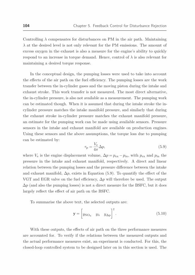
104 Chapter 5. Feedback Control for Disturbance Rejection
Controlling λ compensates for disturbances on PM in the air path. Maintainingλ at the desired level is not only relevant for the PM emissions. The amount ofexcess oxygen in the exhaust is also a measure for the engine’s ability to quicklyrespond to an increase in torque demand. Hence, control of λ is also relevant formaintaining a desired torque response.
In the conceptual design, the pumping losses were used to take into accountthe effects of the air path on the fuel efficiency. The pumping losses are the worktransfer between the in-cylinder gases and the moving piston during the intake andexhaust stroke. This work transfer is not measured. The most direct alternative,the in-cylinder pressure, is also not available as a measurement. The pumping workcan be estimated though. When it is assumed that during the intake stroke the in-cylinder pressure matches the intake manifold pressure, and similarly that duringthe exhaust stroke in-cylinder pressure matches the exhaust manifold pressure,an estimate for the pumping work can be made using available sensors. Pressuresensors in the intake and exhaust manifold are available on production engines.Using these sensors and the above assumptions, the torque loss due to pumpingcan be estimated by:
τp = Ve4π∆p, (5.9)
where Ve is the engine displacement volume, ∆p= pex−pin, with pex and pin thepressure in the intake and exhaust manifold, respectively. A direct and linearrelation between the pumping losses and the pressure difference between the intakeand exhaust manifold, ∆p, exists in Equation (5.9). To quantify the effect of theVGT and EGR valve on the fuel efficiency, ∆p will therefore be used. The output∆p (and also the pumping losses) is not a direct measure for the BSFC, but it doeslargely reflect the effect of air path on the BSFC.
To summarise the above text, the selected outputs are:
y =[yNOx yλ y∆p
]ᵀ. (5.10)
With these outputs, the effects of air path on the three performance measuresare accounted for. To verify if the relations between the measured outputs andthe actual performance measures exist, an experiment is conducted. For this, theclosed-loop controlled system to be designed later on in this section is used. The

5.4. Experimental Design 105
200 300 400 500 600 700 800 900 10000
2
4
6
8
NO
x in g
/kW
h
NOx in ppm
1.5 1.55 1.6 1.65 1.7 1.75 1.8 1.85 1.90
2
4
6
8
10
PM
in m
g/kW
h
λ in [−]
10 15 20 25 30 35 40 45 50 55 60100
101
102
103
104
105
BS
FC
in a
.u.
∆p in kPa
Figure 5.3: The relation between the measured outputs and the actual performanceindicators. The engine speed and fuel injection during the experiment were fixedat 1455RPM and 120mg/inj. The BSFC is converted into arbitrary units for de-identification purposes. For this, the BSFC is multiplied with a constant, such that∆p = 0kPa would correspond with a BSFC of 100 a.u. using a linear extrapolationof the data in gray. The black dots in the above three plots all originate from thesame time-domain data sequence, and similarly for the gray dots.

106 Chapter 5. Feedback Control for Disturbance Rejection
setpoints for the measured outputs are manually varied while maintaining theengine speed and fuel flow constant at 1455RPM and 120mg/inj. The feedbackcontroller then adapts the VGT and EGR valve in accordance with the setpointchanges, which changes the performance tradeoff. For this experiment, the sensorsof the dynamometer setup were used to determine the NOx emissions, PM emissionsand BSFC. The engine sensors were used to measure the selected outputs.
Figure 5.3 shows the results of the experiment. Two data series are shownin the plots. In the black series, the variation is mostly in NOx and λ. Here,a 538% and 696% difference between the lowest and highest value of NOx andPM is observed, respectively. The resulting change in ∆p and BSFC is relativelysmall, compared with the gray data series. In the gray data series, the variationis mostly in the ∆p setpoint. Here, a significant variation in BSFC is observed,with relatively small changes in NOx and PM, compared with the black data series.This shows that ∆p has a significant effect on BSFC. In addition, it indicates thateven large variations of the emissions as a result of changing in-cylinder conditionshave a, by comparison, small effect on the BSFC. This indicates that for theconsidered actuators, the effect of PMEP on the BSFC is stronger than the effectof IMEPg. The PM graph and NOx graph also show the expected relations betweenthe controlled outputs and the high-level performance measures. The intendedrelations between the controlled outputs and the performance measures are allpresent, which indicates that the selected outputs are indeed relevant.
The experiment of Figure 5.3 is only a partial validation of the intendedrelations. With only two actuators, neither the three controlled outputs, nor thethree high-level objectives can be varied independently. Cross-correlations willtherefore affect the results of the experiment. Moreover, it is known from theory(see Chapter 2) that the selected controlled outputs are only partially representativefor the high-level objectives. For example, the start of combustion is known toaffect the NOx, PM and BSFC; and this effect will not be noticeable in the λ and∆p output. Also, when the EGR rate changes, and somehow λ and ∆p maintainconstant, the PM emissions and BSFC will change. These effects are not capturedby the selected outputs.
The important step of modeling the input-output behavior is covered in Chap-ter 4. This section uses the results of Chapter 4 and continues with analyzing theresulting control problem, control design and experimental validation.

5.4. Experimental Design 107
5.4.2 Input-Output Analysis
With only two inputs (VGT and EGR valve) to control three outputs (NOx, λ, ∆p),exact tracking of all outputs and, therefore, functional controllability (Skogestadand Postlethwaite, 2007) cannot be achieved. Instead, the feedback controller isintended to maintain the setpoint values as close as possible to the three outputs,using the two available actuators. The nominal input settings are chosen to result inPareto optimal outputs under nominal stationary conditions. Keeping the outputsclose to the nominal outputs therefore implies the performance is close to optimal.Due to the lack of actuators, only the two-dimensional subspace in which theVGT and EGR valve have control authority is of interest for control design. Inthis section, the input-output controllability properties of the two directions inwhich the VGT and EGR valve have a stationary gain are investigated. The thirddirection, where the actuators have no gain will necessarily remain uncontrolled.
As an alternative to the proposed three-output control problem, a two-outputemission control problem, using only NOx and λ as outputs, is considered in thissection. This control problem is not underactuated and perfect tracking of NOx
and λ can be aimed for. This should result in a reduced spread of the engine-outemissions. Because ∆p is no longer controlled, the fuel efficiency is not takeninto account. The system dynamics of the two-output system are denoted G2(s),whereas in this section the three-output system is denoted G3(s), with s theLaplace operator. The addition of (s) is omitted in the remainder of this sectionfor notational convenience.
To make the system outputs comparable for analysis, output scaling is applied:
yi = SiGiufb = Giufb, (5.11)
where Si is the diagonal scaling matrix for system Gi, the scaled system is denotedGi and the scaled outputs yi, the subscript i∈ {2,3} distinguishes between the twoand three output system. The scaled static system gain is Gss,i = Gi(s= jω = 0),where ω represent the frequency. Figure 5.4 visualizes the scaled static system gainfor the two considered output combinations at mid speed and mid load.
Including ∆p as a third control output improves both the robustness of theperformance and the robustness of the closed-loop stability. These effects arediscussed in the remainder of this section.

108 Chapter 5. Feedback Control for Disturbance Rejection
−10
1
−10
1
−1
0
1
yNOxyλ
y ∆p
−2 −1 0 1 2−2
−1
0
1
2
yNOx
y λ
Figure 5.4: The scaled steady-state response to unit-size inputs. Two outputconfigurations are used. The operating point is 1455RPM and 120mg/inj. The plotsshow: yi = Gss,iufb, ∀ |ufb|2 = 1, for two different systems Gi. On the left, thetwo-output emission system Gss,2 is shown. On the right, this two-output system(light gray) is compared with the three-output system Gss,3 (dark gray).
The BSFC is considered a fundamental part of the engine performance. Main-taining ∆p close to its nominal value by means of feedback control keeps its effecton the BSFC small. This improves the robustness of the BSFC and consequentlyalso of the engine performance. In the two-output system, where ∆p is not con-trolled, the actions of the VGT and EGR valve to control NOx and λ will alsoaffect the ∆p. This induces an additional disturbance on ∆p and hence also onthe BSFC. Including ∆p as a control output therefore improves the robustness ofthe engine performance.
The reasoning for improved closed-loop stability, when ∆p is included, is moretechnical. Its effect on stability can be quantified using the condition number ofthe scaled static-gain matrix. The condition number of the static gain matrix isan important characteristic for MIMO control. It is the ratio between the gains ofthe most sensitive and least sensitive input-output direction. Ideally, the conditionnumber is close to one. A condition number much larger than one indicates thatthe system is close to singular and has a small response in one direction.
The condition number of the scaled static gain matrix is shown in Table 5.3 fora range of operating points and for both output configurations. For G2, the systemresponse is naturally ill-conditioned around the nominal input settings. Seven outof the nine operating points considered in Table 5.3 have a condition number after

5.4. Experimental Design 109
Table 5.3: The condition number, κi, of the scaled static gain matrix, for a rangeof operating points and for both considered output configurations.
ωeng Fuel κ2 κ3
RPM mg/inj
1011 60 22.35 3.39
1011 120 17.79 2.20
1011 200 73.36 1.98
1455 60 8.25 2.27
1455 120 10.24 1.69
1455 200 11.07 1.35
1700 60 11.59 1.87
1700 120 10.59 1.63
1700 200 4.31 2.20
scaling, κ2, larger than 10, with a maximum of κ2 = 73.4. Including ∆p as a thirdoutput reduces the condition number in all operating points. For the three-outputsystem, eight out of nine points have a condition number, κ3, smaller than 2.3.The maximum condition number that is encountered for the three-output systemis 3.39.
The static gain of Gss,2 and Gss,3 at 1455 rpm and 120 mg/inj is visualizedin Figure 5.4. The narrow ellipsoid in the left graph of Figure 5.4 shows that thetwo-output system has a small response in one direction. The more round ellipsoidin the right graph of Figure 5.4 indicates that the three-output system has a similarresponsiveness in all directions in the depicted plane. This shows graphically whythe condition numbers between the two systems differ in magnitude. It is observedthat the difference in the condition numbers is not due to an ill-chosen outputscaling. The magnitude of the response is similar for all three outputs. Instead,the low gain in the direction of simultaneously decreasing NOx and increasing λ isthe reason for the high condition number.
The condition number directly affects the robust stability of the closed-loop.To analyze robust stability, the system uncertainty is modeled. The uncertainty is

110 Chapter 5. Feedback Control for Disturbance Rejection
modeled here as a norm-bounded additive uncertainty:
yi =(Gi+∆i
)ufb, (5.12)
with Gi the nominal dynamic response of the input-output system and the un-certainty ‖∆i‖2 < δ‖Gi‖2. The parameter δ bounds the uncertainty relative tothe spectral norm of the system gain. The uncertainty is only norm-bounded, thedirection of the uncertainty is not specified. An uncertainty of δ = 0.1 is equiva-lent to an uncertainty of 10% of the nominal system response. This uncertaintymodel only roughly approximates the actual system uncertainty, but is useful todemonstrate the effect of conditioning on the closed-loop stability.
The closed-loop system is considered more robust against uncertainties if theallowed δ for which the system is closed-loop stable is larger. Without consideringa specific control design, the condition number can be used to specify a maximumδ for which the uncertain system is input-output controllable. For δ ≥ 1
κ , thestatic gain may become singular and its sign is uncertain. This means that theuncertain system is not robustly functionally controllable; even locally, closed-loop asymptotic stability, taking the system uncertainty into account, cannot beguaranteed by any linear controller.
The uncertainty due to measurement noise and nonlinear behavior was ex-tensively analyzed at the nominal operating point in Chapter 4. Combining theindividual effects of noise and nonlinear behavior on the FRF measurement, andof nonlinear behavior on the actual system response gives a standard deviationof σ ≈ 0.05 of the system response at low frequencies, largely due to nonlineareffects. Uncertainty due to, e.g., aging, changing ambient conditions or productiontolerances is not even taken into account here. When a 2σ uncertainty range isused, which is equivalent to 95% certainty that the actual system response is withinthe uncertainty bounds, this results in δ = 0.1. Consequently, only systems withκ < 10 are robustly functionally controllable when the identification inaccuracy istaken into account.
The G2 system is not robustly functionally controllable in the largest part ofthe operating range, when the model uncertainty is taken into account. For theG3 system, which has a lower condition number, robust closed-loop asymptoticstability can be achieved in two directions for the entire operating range. Because

5.4. Experimental Design 111
this system is underactuated, one direction will remain uncontrolled and the systemis, by definition, not functionally controllable. However, two controllable directionsare present and a robustly stable controller making full use of the VGT and EGRvalve can be designed.
The observations in this section are a direct consequence of having simultane-ously low engine-out NOx and PM emissions. Well chosen control actions can stillsimultaneously decrease NOx and increase λ. But, as can be seen in Figure 5.4,the input direction that achieves this corresponds with a steep increase in ∆p andaccordingly increased BSFC. This is also the reason for the significant improvementof the condition number when ∆p is included as a third output. Even when the ro-bust stability issues are disregarded, the strong effect a NOx-λ controller will haveon ∆p, and hence also on the fuel efficiency, makes NOx-λ feedback control, usingthe VGT and EGR valve, undesirable. It can be expected that, when substitutemeasurements for NOx, λ and ∆p are used, that maintain the desired correlationwith the respective high-level objectives, these conclusions hold as well.
5.4.3 Control Design
In this section, a feedback controller is designed for the 1455RPM, 120mg/inj
operating point. For the design of the feedback controller, static SVD decoupling(i.e. decoupling based on the Singular Value Decomposition of the static systemgain), combined with classical (PI) feedback control is used. The reasons for thisare the following. The identified FRF model (Figure 4.8) is directly suitable forloopshaping control design of classical controllers and the resulting controllers aresuitable for implementation without further processing. Typically, the design effortfor classical controllers is lower than for a model-based control design, becauseseveral difficult steps that are needed to mathematically define and solve the controlproblem can be avoided. The use of decoupling is required due do to the systembehavior, which is strongly coupled as can be seen in Figure 4.8. Static decouplingwill show adequate performance and is much simpler to design and implement thandynamic decoupling. In this section, the design and functioning of the decouplingand feedback controller are elaborated.

112 Chapter 5. Feedback Control for Disturbance Rejection
Decoupling
Decoupling serves a double purpose in the controller, both are accomplished viaSVD decoupling. First, two output directions are separated from a third directionin which the VGT and EGR actuators have no influence. This solves the underac-tuation problem. Second, the two remaining directions are decoupled. This resultsin a diagonally dominant Two-Input, Two-Output (TITO) system.
The design of the decoupling matrices is based on the local static system gain.The two-input, three-output system, G, describes the dynamic response of theengine:
yfb = Gufb, (5.13)
where yfb =[yNOx yλ y∆p
]ᵀand ufb =
[uVGT uEGR
]ᵀ. Now, consider the
diagonal output scaling S∈R3×3, static gain matrix of the system response: Gss =G(ω = 0) ∈ R3×2 and the following SVD decomposition:
S =
0.05 0 0
0 50 0
0 0 0.7
, (5.14)
SGss =
1.4626 −1.0914
0.8916 −1.0040
−1.2722 −0.7582
, (5.15)
UΣVᵀ = SGss, (5.16)
where U ∈ R3×2 and V ∈ R2×2 are orthonormal matrices and Σ ∈ R2×2 is adiagonal matrix. The diagonal scaling matrix S is again used to scale the outputs.It accounts for the difference in units and their importance and can be used totrade performance between the different controlled outputs. Input scaling is notapplied, because both inputs are expressed in % and range between 0% and 100%.Using the results of the SVD decomposition, the TITO system Gd:
ε= UᵀSGVυ = Gdυ, (5.17)
with inputs υ = [υ1,υ2]ᵀ and outputs ε= [ε1,ε2]ᵀ, is obtained that has a diagonalstatic response. The block scheme of Figure 5.5 shows the implementation of the

5.4. Experimental Design 113
yNOx
yλy∆p
uVGT
uEGR
GVU>SC1
rNOx
rλr∆p
−++
υ1ε1
unominal,VGT
unominal,EGR
C2ε2 υ2
Figure 5.5: A block scheme representation of the control architecture.
decoupling in the control scheme. After SVD decoupling, a functionally controllable,decoupled TITO system remains.
The decoupling is designed to exactly match the static input-output gain ofthe nominal system. The dynamic decoupling quality is quantified by calculatingthe Relative Gain Array (RGA) (Skogestad and Postlethwaite, 2007), Λ, of thedecoupled system:
Λ = Gd ◦ (G−1d )ᵀ, (5.18)
where the ◦-symbol is used to denote the Hadamard product (i.e. entry-wiseproduct). Figure 5.6 shows the diagonal and off-diagonal entries of the RGA ofthe decoupled system. Up to and somewhat beyond the intended bandwidth of0.2Hz, the diagonal RGA value is close to one and the off-diagonal RGA value isclose to zero, which indicates that the effects of coupling are small. For the rangeof frequencies that is most of interest for feedback control design, Gd is close tobeing fully decoupled.
Feedback Control Design
Implementing two SISO feedback controllers C1 and C2 results in a closed-loopcontrolled system. For the design of C1 and C2, a variation of sequential loopshaping is used. The parameters of the diagonal PI controller are designed in aniterative loop. The closed-loop effects of the already designed control elementsare taken into account during the design process. Also, the effective closed-loopbehavior of the controlled MIMO system is reviewed during the design process.Interaction between the diagonal terms (i.e. coupling) that remains after SVD-decoupling is thereby accounted for, both for stability and performance.
The PI controller is a good match for the system dynamics due to the low-passcharacteristics found in all transfer functions and the performance requirements

114 Chapter 5. Feedback Control for Disturbance Rejection
Frequency in Hz
Mag
nitu
de
10−1
100
101
0
0.5
1
1.5
2
DiagonalOff−diagonal
Figure 5.6: The diagonal and off-diagonal entries of the absolute values of therelative gain array, |Λ|. The frequency range up to the intended bandwidth of 0.2Hzis shown in gray.
that focus on low frequency performance. The use of a PI controller results insmooth control actions and the controller is guaranteed to eliminate all steady-stateerrors in the controlled directions. The system dynamics did not give cause forusing any additional dynamic elements in the controller. For C1, a PI controllerwas designed, for C2, only integral control was used. The use of the followingcontroller resulted in the desired closed-loop bandwidth of 0.2Hz:
x1
x2
υ1
υ2
=
0 0 1 0
0 0 0 1
0.6 0 3 0
0 2.5 0 0
x1
x2
ε1
ε2
. (5.19)
The expected transient performance can be evaluated using the closed-loopsensitivity, shown in Figure 5.7. The diagonal elements of the sensitivity showthe expected transient performance level when disturbances are present. Theoff-diagonal elements show the effects of coupling. The singular values show theworst case and best case performance. In Figure 5.7, it can be seen that up to0.2Hz, the sensitivity is always below 100. Up to this frequency, the feedback

5.4. Experimental Design 115
10−1
100
101
10−2
10−1
100
Frequency in Hz
Mag
nitu
de
Sensdiag
Sensoff−diag
σ(Sens)
Figure 5.7: The closed-loop sensitivity: Sens = (I+CGd)−1 and σ(Sens): thesingular values of Sens, denoting the best and worst case performance. The sensi-tivity indicates how effective the controller is at counteracting disturbances.
controller improves the tracking performance. Also, it can be observed that theoff-diagonal, cross-coupling elements are relatively small when compared with thediagonal elements, i.e., decoupling was successful.
To check for closed-loop MIMO stability, the generalized Nyquist stabilitycriterion is used. By visual inspection of the Nyquist plot, stability can be assessed.For the used MIMO control structure, the Nyquist plot consists of the real andimaginary part of:
N(jω) = det(I+C(jω)UᵀSG(jω)V) , (5.20)
where C is the diagonal controller of Equation (5.19). Closed-loop stability isobtained when N passes the origin to the right, while following N from low to highω. The minimal distance of N to the origin is an indication for robustness, wherea larger distance is equivalent to a more robust closed-loop. Standard practiceis to use at least a radius of 0.5 around the origin. For the designed controller,a minimum distance of 0.72 was found, while obtaining the desired bandwidth.This indicates that the closed-loop stability is robust against an uncertain sys-tem response. The large robustness margin would also allow for increasing theclosed-loop bandwidth beyond the target bandwidth, to further improve the high-frequency disturbance rejection. However, considering the frequency content of the

116 Chapter 5. Feedback Control for Disturbance Rejection
−3 −2 −1 0 1−2
−1
0
<(N)
=(N)
Figure 5.8: A Nyquist plot, showing the real and imaginary part of N . The circlewith radius 0.5 shows the region that should be avoided to achieve robust stabilitywith a modulus margin of at least two.
disturbances, this is not expected to bring significant improvements of the overallemissions or fuel efficiency. Therefore, the good robustness properties and smoothinputs associated with the large robustness margin are preferred over an increasedbandwidth.
It is shown here that the dynamic response of the NOx-sensor is sufficientlyfast for obtaining the desired transient performance. With a faster sensor, themeasured NOx dynamics would have been faster. This would have made the staticapproximation used for decoupling useful in a larger frequency range, which wouldlikely have given further improvements of the decoupling quality. Furthermore,it would have allowed for a higher closed-loop bandwidth. However, the desiredperformance level (closed-loop bandwidth) can be achieved using the current sensor.This makes the selection of suitable reference values and the accuracy of themeasurements the most important factors that determine the resulting engineperformance. Considering that the encountered disturbances are all low frequent,the current controller is sufficiently fast to adequately counteract them. Therefore,tracking the same references even more accurately, using the same sensors, butusing a more advanced control algorithm with a higher bandwidth, is not expectedto significantly improve the engine performance.

5.4. Experimental Design 117
5.4.4 Experimental Results
The controller designed in Section 5.4.3 is implemented on a test engine mountedon a dynamometer test setup. The engine and test setup are the same as the onesused for identification in Chapter 4 and described in Section 4.2.
To test the performance of the feedback controlled engine, disturbances areapplied. Aging and fouling of the engine and changing ambient conditions arealways present, but difficult to influence during the experiment. Therefore, distur-bances are applied in other parameters that can be influenced to act in place ofthe actual disturbances. Step disturbances are applied to the nominal VGT andEGR settings. Also, the engine speed and load are changed from their nominalvalues. These artificial disturbances do not correspond with any specific actualdisturbance, but do show the response of the controlled engine to disturbances.
For this test of the feedback controlled engine, the disturbances are appliedas steps, whereas the actual disturbances are slowly varying. These step-wisedisturbances are more suitable for demonstrating the transient performance ofthe controller. When the test was executed with slowly varying disturbances, thecontroller would be in quasi-stationary state at all times and the actual transientresponse would not be visible. The transient performance of the controller is ofimportance despite the slowly varying nature of the disturbances. Due to thecontinuously changing engine speed and load, fast and dynamic adaptations areneeded.
The presented experiments are conducted in the neighborhood of a nominaloperating point: 1455RPM and 1050Nm. For the test engine, this point is closeto the center of the speed and load operating range. The engine load is controlledin open loop, using the fuel flow. Because the disturbances all have a small effecton the fuel efficiency and hence the produced torque, the load is not completelyconstant when the disturbances are applied. Feed-forward control schemes, nor-mally used to adapt the VGT and EGR valve during engine speed or load changes,are not active during this experiment.
The tests should experimentally verify the following questions.
• Asymptotic stability; does the closed-loop controlled engine converge tosteady state; is the closed-loop system asymptotically stable?

118 Chapter 5. Feedback Control for Disturbance Rejection
• Transient response; how long does it take before steady state is reached; isthe desired bandwidth achieved?
• Engine performance; does the engine performance suffer from the under-actuation?
Figure 5.9 shows the experimental results for input disturbances and Figure 5.10shows the results for engine speed and torque disturbances. The figures show thethree measured outputs, two decoupled errors, ε, two inputs and the speed-loadoperating point. In both figures, it is observed that the engine converges to a stableequilibrium after a disturbance is applied in all cases. The feedback controller makesthe controlled errors, ε, return to zero asymptotically. The error remains close tozero as long as no new disturbance is applied. This shows closed-loop asymptoticstability. Also, it demonstrates robust stability against model uncertainty and theapplied disturbances.
The transient response time that is observed after a step disturbance is appliedis under 5 s in all cases. The transient response after a disturbance in torque(Figure 5.10) is slightly slower than after a disturbance in the VGT or EGRvalve (Figure 5.9). The instantaneous torque disturbance evokes a dynamic effect,therefore, in the air path the disturbance is not perceived as a step.
The disturbances that are applied in the input values, VGT and EGR valve,are counteracted completely, as can be seen in Figure 5.9. These disturbances are,by definition, exactly in the direction in which the VGT-EGR valve controller hascontrol authority. Underactuation is therefore not an issue. When the feedbackcontroller exactly counteracts the disturbances in ε, the original equilibrium isrecovered and perfect tracking of all three outputs is achieved. With all disturbancesexactly eliminated, the achieved engine performance in terms of NOx emissions,PM emissions and BSFC can be expected to match the nominal performance.
The disturbances in the operating point (torque and engine speed), shownin Figure 5.10, cannot be counteracted completely. When the operating pointis changed, it is no longer possible to maintain the exact same NOx, λ and ∆psimultaneously by adapting the VGT and EGR valve. Nonetheless, ε alwaysconverges to zero, which means that within the capabilities of the VGT and EGRvalve the closest possible tracking is achieved.

5.4. Experimental Design 119
300
400
500
600
NO
x in p
pm
actualreference
1.6
1.8
2λ
actualreference
20
30
40
50
∆ p
in k
Pa
actualreference
−40
−20
0
20
40
ε
ε 1ε 2
30
35
40
45
50
VG
T in
%
actualfeed forward
30
35
40
45
50
55
EG
R in
%
actualfeed forward
1300
1400
1500
1600
Eng
ine
spee
d in
RP
M
0 20 40 60 80 100800
900
1000
1100
1200
1300
Tor
que
in N
m
Time in seconds
Figure 5.9: Rejection of step disturbances using feedback control. From top tobottom: the measured outputs (NOx, λ, ∆p), decoupled outputs (ε), inputs (VGTand EGR) and operating point (Engine Speed, τ). Disturbances are applied first inthe EGR valve at time=0 s and in the VGT actuator at time=50 s.

120 Chapter 5. Feedback Control for Disturbance Rejection
300
400
500
600
NO
x in p
pm
actualreference
1.6
1.8
2
λ
actualreference
20
30
40
50
∆ p
in k
Pa
actualreference
−40
−20
0
20
40
ε
ε 1ε 2
30
35
40
45
50
VG
T in
%
actualfeed forward
30
35
40
45
50
55
EG
R in
%
actualfeed forward
1300
1400
1500
1600
Eng
ine
spee
d in
RP
M
0 50 100 150 200800
900
1000
1100
1200
1300
Tor
que
in N
m
Time in seconds
Figure 5.10: Rejection of engine speed and torque disturbances using feedback con-trol. From top to bottom: the measured outputs (NOx, λ, ∆p), decoupled outputs(ε), inputs (VGT and EGR) and operating point (Engine Speed, τ). Disturbancesare applied first in load at time=0 s and in engine speed at time=90 s.

5.4. Experimental Design 121
Particularly the disturbances in torque leave a noticeable difference betweenthe reference values and measured values for all three outputs. Increasing torquewill increase NOx, decrease λ and increase ∆p. All three of these changes areundesirable, but the tradeoff between the three outputs is effectively maintained.The remaining error is distributed over all three outputs, which is preferred overexact tracking of only two outputs. Decreasing torque has the opposite effect, andsimultaneous improvements in NOx, λ and ∆p are obtained and again the tradeoffbetween the three outputs is maintained. This is not a coincidence; the directionin which the VGT and EGR valve have no control authority is perpendicular tothe dark grey ellipsoid of Figure 5.4. This direction will always correspond withthe direction of the remaining static error.
The disturbances in engine speed are not applied instantaneously, because theacceleration capabilities of the test cell are physically limited. The disturbances asa result of the applied speed changes are counteracted with very small errors. Theadaptations needed in VGT and EGR valve are significant, but in the NOx, λ and∆p signals, almost no change can be observed. Apparently the direction of thedisturbances matches the directions where the VGT and EGR valve have controlauthority. Hence, the VGT and EGR controller can almost perfectly counteractthis disturbance.
To summarize the results, the three research questions posed earlier in thissection are answered.
• Asymptotic stability; the experiments verify that the closed-loop controlledsystem is asymptotically stable in this operating point and robustly stablefor the applied disturbances.
• Transient response; the transient response after a step disturbance confirmsthat the desired bandwidth of 0.2Hz is achieved.
• Engine performance; except for the torque steps, the tracking performanceis very good. The steady-state errors in NOx, λ and ∆p are very small. Fortorque steps, an error remains that is outside the control authority of theVGT and EGR valve, but the desired tradeoff between emissions and fuelefficiency is maintained. The engine performance therefore remains close tonominal in all tested circumstances.

122 Chapter 5. Feedback Control for Disturbance Rejection
The experiments show that a robustly stable and fast feedback controller isdesigned. The controller maintains the desired tradeoff between emissions and fuelefficiency and counteracts disturbances with small tracking errors in NOx, λ and∆p.


6 Efficient Control Design forLow Emission, Fuel EfficientDiesel Engines
125
In the previous chapter, a feedback controller was designed. It is shown that thiscontroller successfully counteracts disturbances, which reduces the spread on theNOx and PM emissions and fuel efficiency. For practical applications, where speedand load variations are present, the controller of Chapter 5 is not directly suitable.The controller was designed to reduce the effects of disturbances, while maintainingclose to a stationary speed-load operating point. Its design is based on a linearmodel, which is accurate only at a single operating point. Therefore, outside ofthis operating point, stability and performance of the controller are not guaranteed.Also, the VGT and EGR valve play an important role when the driver torquedemand varies. To realize these torque variations with low emissions, fast changesin the air and exhaust flows are needed. The VGT and EGR valve should beused actively to change the air and exhaust flows in accordance with the changingtorque demand. The controller of Chapter 5 does not accommodate this.
This chapter deals with efficiently designing a controller that is suitable towork on the entire speed-load operating range and addresses the above issues. Thedesign procedure for the feedback controller is adapted, such that stability andperformance in the entire operating range are taken into account. Also, a dynamicfeed-forward controller is designed and implemented to provide additional air-pathcontrol actions during torque transients.
The complexity of the control design is intentionally kept low to reduce thedesign and implementation effort, which is a considerable problem in current enginecontrol design. Production controllers use maps that determine actuator settings oradjustments to these actuator settings depending on the operating point and sensor
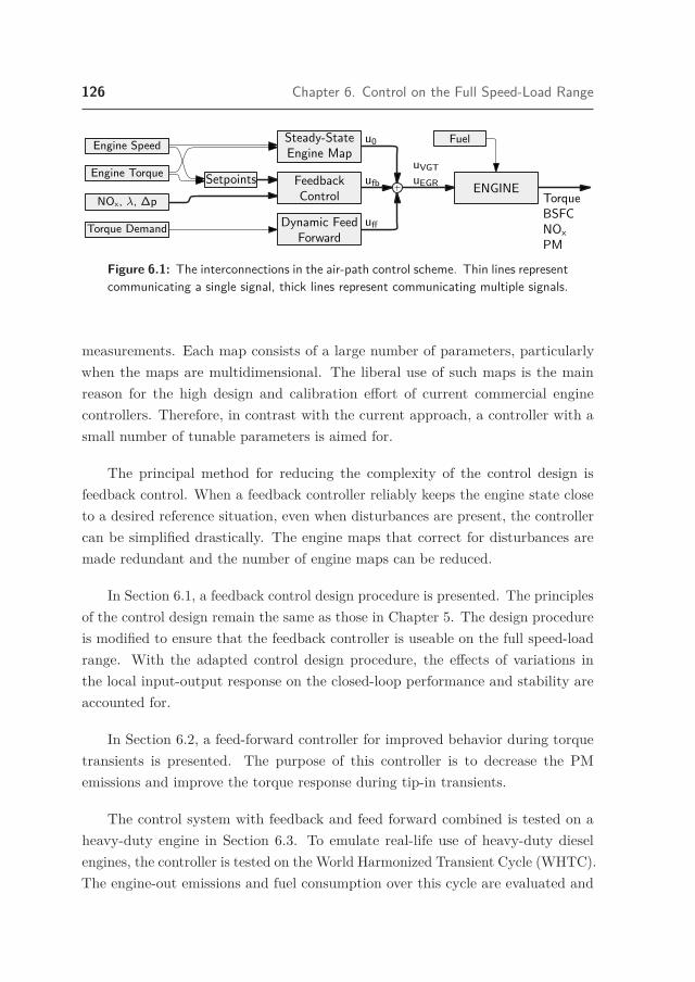
126 Chapter 6. Control on the Full Speed-Load Range
uVGT
uEGR ENGINESetpoints
Engine Speed
NOx, λ, ∆p
Engine Torque
Fuel
FeedbackControl
Dynamic FeedForward
Torque Demand
u0
ufb
uff
Steady-StateEngine Map
TorqueBSFCNOx
PM
Figure 6.1: The interconnections in the air-path control scheme. Thin lines representcommunicating a single signal, thick lines represent communicating multiple signals.
measurements. Each map consists of a large number of parameters, particularlywhen the maps are multidimensional. The liberal use of such maps is the mainreason for the high design and calibration effort of current commercial enginecontrollers. Therefore, in contrast with the current approach, a controller with asmall number of tunable parameters is aimed for.
The principal method for reducing the complexity of the control design isfeedback control. When a feedback controller reliably keeps the engine state closeto a desired reference situation, even when disturbances are present, the controllercan be simplified drastically. The engine maps that correct for disturbances aremade redundant and the number of engine maps can be reduced.
In Section 6.1, a feedback control design procedure is presented. The principlesof the control design remain the same as those in Chapter 5. The design procedureis modified to ensure that the feedback controller is useable on the full speed-loadrange. With the adapted control design procedure, the effects of variations inthe local input-output response on the closed-loop performance and stability areaccounted for.
In Section 6.2, a feed-forward controller for improved behavior during torquetransients is presented. The purpose of this controller is to decrease the PMemissions and improve the torque response during tip-in transients.
The control system with feedback and feed forward combined is tested on aheavy-duty engine in Section 6.3. To emulate real-life use of heavy-duty dieselengines, the controller is tested on the World Harmonized Transient Cycle (WHTC).The engine-out emissions and fuel consumption over this cycle are evaluated and

6.1. Feedback Control 127
compared with the values that are achieved with a production-type EURO VIcontroller.
The contents of this chapter are largely based on Criens et al. (2014).
6.1 Feedback ControlThe purpose and design principles of the feedback controller are the same as thosein Chapter 5. To recapitulate, the purpose of the feedback controller is to maintainthe BSFC, NOx emissions and PM emissions at all times as close as possible tothe values obtained under nominal conditions. The control design of Chapter 5needs to be modified to accommodate speed and load variations, which were notconsidered in Chapter 5. The required modifications are discussed in this section.
In Chapter 4, it was shown that the encountered local input-output behaviorcan be accurately represented by a linear model (Figures 4.6 and 4.7). However,it was also shown that the local input-output behavior varies significantly, whenthe speed-load operating point changes (Figure 4.8). Amplitude variations of afull order of magnitude and sign changes are observed. A controller designed usingonly the input-output response at a single operating point can therefore not beexpected to function in the entire speed-load range.
To take the nonlinear behavior into account, several control design methodscan be used. In order of increasing complexity, the following control design methodscan be considered.
• Linear control design, taking into account the variations of in the localbehavior for both stability and performance, without dynamically adaptingthe controller properties.
• Gain-scheduled control design, adjusting the controller parameters onlinefor the known variations in the local behavior.
• (Quasi) linear parameter varying control design, explicitly taking into ac-count the time-varying nature of the input-output behavior.
• Nonlinear control design, where a nonlinear controller is designed using anonlinear engine model, which desribes the full engine behavior.

128 Chapter 6. Control on the Full Speed-Load Range
Considering the goal to produce an efficient control design, the linear controldesign method is preferred. Linear control is the least complex, both in terms of thedesign procedure and the implementation. It is however also the most conservative.Considering the large variations that are present in the input-output behavior, itmight not even be possible to achieve closed-loop asymptotic stability with a linearcontroller. In this section, the design of a linear controller for feedback control inthe entire operating range is elaborated. It is shown that stability and convergenceto small tracking errors can be achieved.
Similar to the controller in Chapter 5, the new controller combines decouplingwith classical control design. The design will be described briefly, focussing on theadaptations needed to accommodate the variation of the input-output behavior atdifferent operating points.
6.1.1 NOx Measurement
A small change is made to the selection of controlled outputs; in particular tothe output representing the NOx emissions. In Chapter 5, the feedback controllerused the NOx concentration as a controlled output, which is measured directlyby the NOx sensor. With a change in the software interacting with the engine,additional measurements became available for the control system, allowing for anadaptation. In this chapter, the brake specific NOx emissions expressed g/kWh arecontrolled. Using the measured air flow, fuel flow, brake torque1 and engine speed,the measured NOx concentration in ppm is converted into the specific engine-outNOx emissions in g/kWh. This conversion has the following advantages.
• Correct for changes in air flow The NOx concentration decreases whenthe the air flow increases while NOx mass flow remains constant. This isunwanted and the specific NOx flow in g/kWh is not affected by this.
• Relation with emission legislation The EURO VI legislation for HD dieselengines imposes a limit on the tailpipe NOx emissions expressed in g/kWh.Using the same units to control the engine-out NOx emissions makes thevalues directly comparable.
1This measurement is not available on production engines and should therefore be replacedwith an estimate.

6.1. Feedback Control 129
• Interpretation When expressed in g/kWh, the NOx value is more natural tointerpret and its nominal value changes less over the speed-load range, whichmakes selecting or adapting setpoint values for NOx more insightful.
Disadvantages of using the specific NOx emissions, rather than the NOx con-centration exist as well. In particular when the brake torque becomes low, zeroor negative, even low NOx mass flows expressed in g/s can result in very highor negative values, when expressed in g/kWh. In this region however, the use ofthe NOx concentration sensor itself can be problematic as well. The NOx sensorrequires a minimum exhaust gas temperature to function, which is not alwaysavailable during warm-up or at low loads. Considering that at low loads, the NOx
and PM emission flows (expressed in g/s) are very low for a wide range of inputsettings, feedback control is disabled below 300 Nm, which prevents these poten-tial issues. Also, because multiple sensors are involved in the conversion of theNOx concentration into the brake specific NOx emissions, inaccuracies in all thesesensors influence the end result. This reduces the relative accuracy of the brakespecific NOx measurement, compared with the NOx concentration measurement.The advantages mentioned earlier make the choice for the brake specific NOx
emissions fundamentally more relevant. The inherent disadvantages are thereforeaccepted.
6.1.2 Decoupling
Similar to the earlier control designs, the design of the decoupling is based on theSingular Value Decomposition (SVD) of the static gain matrix. This gain matrixfollows directly from the system identification. Because the input-output responseis operating point dependent, the static gain matrix is as well. But, as will beshown, fixed, static decoupling matrices can again be used to effectively decouplethe input-output system for the entire operating range. For the design of thecontroller and decoupling, 35 operating points are considered. The distribution ofthe operating points is shown in Figure 6.2. The operating points span the entireoperating range, except for the very low torque range. The operating points arenot distributed evenly over the range. To allow for a more detailed analysis of thelocal variation in the frequency response, the distribution is locally more denseat some points. Only nine operating points are used to graphically present theresults in this chapter to prevent cluttering of the graphs with too many lines. All

130 Chapter 6. Control on the Full Speed-Load Range
0 500 1000 1500 20000
50
100
150
200
250
Engine speed in RPM
Fue
l val
ue in
mg/
inj
Figure 6.2: The operating points used for design and analysis of the controller. The’x’-markers show all considered operating points. The circles indicate the selectedoperating points for the figures in this section.
identified points are used for design and analysis of the controller. For design ofthe decoupling matrix, first an average static gain matrix is calculated using:
G = sgn(<(G1(0)))◦(
N∏n=1|Gn(0)|
) 1N
≈
0.2548 −0.2728
0.0130 −0.0214
−1.9714 −1.2263
, (6.1)
where ◦ denotes the Hadamard product (i.e. entry-wise product), also theproduct and the 1/N power are performed entry-wise. The index n represents theoperating point, N the number of operating points, i.e., N = 35, Gn the identifiedFRF at operating point n and <(G1(0)) the real part of the static gain matrixat a nominal operating point (1455 rpm, 120 mg/inj), which is used to recoverthe sign of the response that is lost when the geometric mean is calculated. Theoutcome G is the geometric-mean static gain. To determine the static gain Gn(0)of system n from the measured FRF, the input-output gain at the lowest frequencyexcited during identification (0.028Hz) is used. In Figure 4.8, it is observed thatthe system gain is close to static here.

6.1. Feedback Control 131
Before decoupling, output scaling is applied, which is adapted due to thechange in outputs compared with the controller of Chapter 5:
Gs = SG =
5 0 0
0 50 0
0 0 0.7
G, (6.2)
where S is again a fixed, diagonal scaling matrix. The chosen values account forthe difference in units and the tracking performance tradeoff between the threedifferent outputs.
The system Gn is decoupled by pre- and post-multiplying with the appropriatescaling and decoupling matrices that are calculated via an SVD:
Gs = U Σ Vᵀ, (6.3)
ε= Gd,nυ = UᵀSGnVυ, (6.4)
where U ∈ R3x2, V ∈ R2x2 and Σ ∈ R2x2, such that UUᵀ = I, VVᵀ = I and Σ isdiagonal. The variables ε and υ represent the outputs and inputs of the decoupledsystem, Gd,n, respectively. When the system response, Gn, is close to G, Gd,n
is close to the diagonal matrix Σ and the system is close to being completelydecoupled.
The system gain is both frequency and operating-point dependent, whichaffects the decoupling quality. To quantify to what extent the actual system isdecoupled, the relative gain array, Λ) (Skogestad and Postlethwaite, 2007), of thedecoupled system is calculated for all operating points and frequencies:
Λn(jω) = Gd,n(jω)◦ (G−1d,n(jω))ᵀ. (6.5)
Figure 6.3 shows Λn(jω), using the local responses shown in Figure 4.8. Itshows that for frequencies up to 0.5Hz, the local behavior is diagonally dominantat all operating points. The large differences in the local behavior, even including asign change in the input-output gain, do not significantly affect the low-frequencydecoupling quality. A closed-loop bandwidth of around 0.2Hz is aimed for, and upto this frequency, neither the dynamic behavior, nor the operating point variationssignificantly decrease the decoupling quality for the purpose of feedback control,

132 Chapter 6. Control on the Full Speed-Load Range
10−1
100
101
0
0.5
1
1.5
2
Frequency in Hz
|Λ|
Figure 6.3: The relative gain array of the decoupled system, Gd,n. In black thediagonal elements, in gray the off diagonal elements. The operating points are thesame as in Figure 4.8.
as is shown in Figure 6.3. Hence, static SVD decoupling with the chosen, fixedmatrices effectively decouples the local input-output dynamics in all operatingpoints.
6.1.3 PI control
The PI feedback controller is designed to achieve maximum bandwidth, whilesatisfying the Nyquist stability criterion, and keeping the sensitivity peak below2 for the entire operating range. Similar to the local control design of Chapter 5,sequential loop-shaping is used to design two PI controllers. Considering the low-pass behavior that characterizes the local input-output response in all operatingpoints, PI control is a suitable structure. The main difference with the design inChapter 5 is that the PI controller is designed to work in the entire operatingrange. Instead of shaping only the frequency response at a single operating point,the frequency response at all identified operating points is shaped simultaneously,according to the above criterion. This way, local stability and performance in alloperating points is accounted for.

6.1. Feedback Control 133
−3 −2 −1 0 1−2
−1
0
<(N)
=(N)
Figure 6.4: The Nyquist plot, calculated on the 3x3 grid of operating points usedalso in Figure 4.8. The black line closest to the circle corresponds with the lowspeed, high load operating point. This operating point is the closest to the stabilitymargins.
The controller is described by:
xfb,1
xfb,2
υ1
υ2
=
0 0 0.6 0
0 0 0 1.2
1 0 0.5 0
0 1 0 0.05
xfb,1
xfb,2
ε1
ε2
. (6.6)
Using this controller, the maximum singular value of the sensitivity is below 0 dBup to a frequency of 0.16Hz for all operating points. The maximum singular valueof the sensitivity is below 2 for all operating points and all frequencies. The 0.2Hzbandwidth target that was formulated in Chapter 5 is not met. But the achieved0.16Hz bandwidth still results in a closed-loop response that is much faster thanthe considered disturbances (see Section 5.2). The generalized Nyquist criterionis used for visually checking stability and robustness against uncertainties in thelocal dynamic response. The Nyquist plot of:
Nn(jω) = det(I+C(jω)UᵀSGn(jω)V) , (6.7)
shown in Figure 6.4, passes the origin to the right, with an amplitude margin of afactor two to provide the desired robustness, when following the line from low to

134 Chapter 6. Control on the Full Speed-Load Range
high frequency. The closed-loop system is therefore locally stable in all consideredoperating points. This is not a definitive proof of stability for the actual systemwith time-varying engine speed and load. A mathematically conclusive proof ofstability with time-varying operating points requires an accurate model of theengine behavior during operating point transients. The identified FRF modelsused for control design only capture the local input-output dynamics and are notvery suitable for modeling the effects of time-varying operating points. Even acommon Lyapunov function that shows stability in all operating points is nota sufficient proof of stability. During speed and load changes, the input-outputresponse will be different than the response at stationary operating points. Stabilitywith time-varying operating points is therefore tested and shown experimentally.
6.1.4 Implementation
Nominal Inputs and Setpoint Values
A practical implementation of the feedback controller requires nominal input set-tings and setpoint values for all outputs. The nominal input settings are de-signed for optimal stationary performance. The accompanying setpoints reflect theachieved engine performance under nominal conditions. Both the nominal inputsand the setpoint values are provided in the form of a lookup table with enginespeed and torque as inputs and the corresponding setpoint value as output. Inbetween the grid points of the lookup table, linear interpolation is used.
For the VGT and EGR valve inputs and the ∆p and λ outputs, a map withnominal values in the form of the above described lookup table was available.For the NOx-output, such a map was not available. Instead, the setpoint valuewas fixed at 3.5 g/kWh. This value does not exactly match to the nominal enginecalibration over the operating range. Considering that the controlled output valueis expressed in g/kWh, and thereby scaled for the engine power, the selected constantvalue is suitable in the entire operating range. The remaining difference acts as adisturbance during the experiments.

6.1. Feedback Control 135
Safety
To ensure safe and stable operation under all encountered circumstances, somemodifications to the feedback controller are made for the practical implementation.This way, a proof-of-concept experiment can be conducted safely, without riskingengine damage in case of controller failure. The feedback controller is disabled inthe low torque range and safety limits are implemented to prevent feedback controlactions that can potentially damage the engine. This is discussed below.
In Section 6.1.1, it was already noted that to prevent issues with the NOx
measurement, the controller should be disabled at low loads. Therefore, at loadsbelow 300Nm and whenever a required sensor measurement is not available, thefeedback controller is disabled. This is implemented by overriding the value of ε andsetting it to zero, whenever the load is below 300Nm or any of the sensors does notoutput a measurement. By setting the input to the controller to zero, the controllerstates xfb and hence the integral action of the controller remain at a fixed value.It can be assumed that by using constant integral action, the controller is stillpartly effective at counteracting the effects of constant disturbances. Maintainingthe integral effect is therefore favorable, compared with setting the output of thefeedback controller to zero. In this low torque range, a low NOx mass flow (in g/s)is combined with a high λ and low ∆p. This can be verified in Section 6.3. In atypical drive cycle that combines low, medium and high torque, it can be expectedthat the contribution of the low torque range to the overall emissions and fuelconsumption is relatively small. Therefore, the overall emissions and efficiency ofthe engine are not significantly influenced by disabling the feedback controller inthe low-load operating range.
Also, two precautions are taken that limit the allowed range of the feed-back control actions. First, the outputs of the feedback controller are limited toufb,i ∈ (−10%,10%). This ensures that the actuators remain in the range wherethe engine behavior is close to linear. Sensor measurements that deviate enoughfrom the nominal situation to require feedback actions outside of this range can oc-cur during fast torque transients, when large disturbances are present, or when anactuator or sensor is malfunctioning. In case of malfunctioning, the implementedoutput limits reduce the probability and consequences of unstable closed-loopbehavior.

136 Chapter 6. Control on the Full Speed-Load Range
Second, anti-windup is applied to ensure that the internal state of the integra-tors in the controller cannot reach excessive values when the controller is saturated.The state of the integrators is limited to xfb,i ∈ (−10%,10%).
The output saturation and anti-windup can limit the effectiveness of the feed-back controller when large disturbances are present that require control actionsoutside of the allowed range. However, to ensure safe operation, they are essential.
6.1.5 Experimental Results
To test the functioning of the feedback controller, the controller is implemented onthe dynamometer test setup described in Section 4.2. The dSPACE AutoboxR© isused as an I/O board for both controlling the actuators and collecting the sensorsignals. The inputs and outputs of the engine are monitored, while the operatingpoint is varied.
Figure 6.5 shows a typical sample from these tests, where the operating pointchanges from medium torque at high engine speed towards high torque at lowengine speed with various in-between points. Linear interpolation with a 20 s slopetime is used when changing the operating point.
In the ε signal, it is observed that ε remains close to zero, when the operatingpoint is constant; and converges to zero quickly after the operating point haschanged. This indicates that the closed-loop behavior is asymptotically stable forthe studied conditions. In the NOx, λ and ∆p signals, it is observed that theactual outputs follow their respective setpoint values. Considering the 0.16Hzclosed-loop bandwidth, approximate first-order behavior at low frequencies and20 s operating-point changes, a remaining error in the order of 31% can be expectedduring the applied operating point changes.
At some points, particularly between 450 s and 475 s, an oscillation in the VGT,ε and ∆p signals can be observed. It was found that this oscillation is related tothe VGT actuator. It is however not caused by the new feedback controller; theoscillation can also occur when fixed input settings are used, or even when a Notchfilter is used to actively counteract input oscillations at the particular frequency.
The discrepancy between the NOx setpoint value and the engine-out NOx
value using nominal input settings acts as a disturbance on the closed loop, which

6.1. Feedback Control 137
1000
1500
2000
2500ω
in r
pm
1000
1500
2000
2500
τ in
Nm
0
5
NO
x in g
/kW
h
1
1.5
2
λ in
[−]
30
40
50
60
∆p in
kP
a
−4−2
024
ε in
a.u
.
20
40
60
80
EG
R in
%
0 100 200 300 400 50030
40
50
60
VG
Tin
%
Time in seconds
Figure 6.5: Testing the behavior of the closed-loop controlled engine. In the NOx,λ and ∆p plots, the gray line denotes the reference value, the black line the actualvalue. In the ε plot, the gray and black line denote ε1 and ε2, respectively. In theEGR valve and VGT plots, the gray line denotes the nominal value, u0, the blackline the actual value, u0 +ufb.

138 Chapter 6. Control on the Full Speed-Load Range
is compensated for by the VGT and EGR valve. The inputs therefore do notnecessarily remain very close to their nominal settings, even in steady state. In bothinputs, smooth behavior is observed. No signs of oscillations, or other indicatorsof being on the verge of instability are observed.
The experiments indicate that the expected stable closed-loop behavior anddisturbance rejection are achieved, albeit only in the torque range above 300Nmdue to the applied restrictions on the feedback controller. Only relatively slowchanges of the operating point were considered in this section. Fast changes of theoperating point are considered in Section 6.2, where additional control componentsare designed and implemented to better accommodate these fast changes.
6.2 Feed-Forward ControlDuring fast tip-in transients, torque buildup can be hampered by the availability ofoxygen, while the turbocharger is accelerating. The injection of fuel is restricted bya smoke limiter, which prevents the injection of more fuel than can be combustedwithout visible smoke. This limitation can prevent compliance with the drivertorque demand, in particular during fast tip-in transients, which has a negativeimpact on the drivability. Besides activating the smoke limiter, the lack of oxygenduring these transients also increases the engine out PM emissions. By adaptingthe VGT and EGR valve, the flow of fresh air, and thereby the availability ofoxygen, can be increased. This way, air-path control can improve the drivabilityand decrease the PM emissions.
Control for improved transient performance differs significantly from the distur-bance rejection considered in the previous section. The encountered disturbancesdue to changes in operating point can be much larger and their timescale is muchfaster. Moreover, the operating point changes are known with the availability ofpedal position and engine speed. These properties favor the use of feed-forwardcontrol over feedback control. Feed-forward control, here, means that control ac-tions are based directly on the operating point, rather than on internal enginesensor measurements.
The goal of the feed-forward controller is to achieve a fast, smooth and mono-tonic torque response, while avoiding excessive NOx or PM emissions. For a HD

6.2. Feed-Forward Control 139
diesel engine, a two second response time to a step change in torque demand isconsidered acceptably fast. To achieve this, a temporary increase in the engine-outNOx and PM emissions must be tolerated. Although without additional controlactions, a temporary increase in the EGR flow and decreased availability of oxygenreduce the NOx emissions during tip-in transients; as a result of control actions re-quired to increase the fresh air flow, an increase in NOx emissions will be observed.The feed-forward controller should ensure that a suitable tradeoff between theNOx and PM increase is made. In this thesis, a moderate increase in the engine-out NOx emissions (up to 25% compared with the steady-state value), combinedwith a necessarily larger increase in the PM emissions is considered a suitabletradeoff during a fast transient. The feed-forward controller will be designed suchthat via tuning of its parameters the NOx-PM tradeoff can be influenced and arange of NOx-PM combinations can be achieved. This makes the structure of thefeed-forward controller applicable independent of the desired tradeoff.
Using the VGT and EGR valve, two measures can be taken to improve thetorque response and decrease the PM emissions. First, decrease the time neededfor the turbocharger to spin up by temporarily increasing the turbine flow andincreasing the pressure difference over the turbine, which increases the turbinepower. Second, increase the fresh air flow by temporarily decreasing the EGR flowuntil the turbocharger speed is sufficient to provide the required boost pressure.These measures improve the torque response and reduce the PM emissions. Simul-taneously, as a result of these actions, the pumping work increases and the EGRflow decreases. Consequently, temporarily the BSFC and NOx emissions increase.Therefore, a tradeoff between low PM emissions and a fast torque response versuslow NOx emissions and a low BSFC exists.
It is worth noting that the goal of feed-forward control is not to improvethe tracking of the stationary setpoints during the torque transient. The optimalsteady-state tradeoff between NOx, λ and BSFC, that is reflected by the NOx, λ and∆p setpoints, is necessarily shifted to improve the fresh air flow and turbochargerresponse during torque transients. Exact tracking of these steady-state setpointsis therefore not equivalent with achieving the optimal transient response. This isalso found in Grahn et al. (2013).
Various solutions for improved transient control found in literature are de-scribed in Section 3. With a goal of optimizing for the emissions, fuel consumption

140 Chapter 6. Control on the Full Speed-Load Range
and torque response directly, while aiming for a fast and efficient control design,model based approaches become impractical. The emissions are difficult to modelaccurately during large transients and for a large range of actuator settings. Thenecessary complexity of such an emission model complicates direct control designusing this model. Also, the large identification effort that can be expected increasesthe control design effort. Moreover, model based approaches that are found inliterature use numerical optimization (Benz, 2010; Sequenz et al., 2011), but thesesolutions are not suitable for real-time implementation. Also, the optimal controldesign of Alberer and Del Re (2009) is not suitable for real-time implementation,without prior optimization on the specific drive cycle.
As a solution, manual calibration of the parameters of a dynamic feed-forwardcontroller is proposed. The general structure of the controller is chosen suchthat it can emulate results obtained via optimal control (Sequenz et al., 2011;Tienstra, 2013). The design and calibration of the feed-forward controller arefurther described in the remainder of this section.
6.2.1 Control Design
The general structure of the proposed feed-forward controller is a linear second-order high-pass filter. This filter is used to generate a feed-forward signal basedon the torque demand. The response of a high-pass filter to a step change in theinput is an immediate output change followed by a smooth decay to zero. Thisresembles the shape of the desired response of both the VGT and EGR to a stepin torque (Sequenz et al., 2011; Tienstra, 2013). To facilitate online tuning ofthe feed-forward characteristics, two parameters are available that determine theproperties of the high-pass filter. The filter takes the following form:
xFF,1
xFF,2
uFF,i
=
−1.5αT,i −αT,i αT,i
αT,i 0 0
0 −αg,i αg,i
xFF,1
xFF,2
τd
. (6.8)
The torque demand in %, τd, is the input to the filter and the feed-forwardcontrol signal, uFF,i, is the output for actuator i ∈ {EGR,VGT}. The two param-eters αT,i and αg,i are used to adapt respectively the gain and time scale of the

6.2. Feed-Forward Control 141
0 2 4 6 8 10
0
0.5
1
1.5
uFFin
%
Time in seconds0 2 4 6 8 10
Time in seconds
Figure 6.6: The effect of changing the parameters αT,i (left) and αg,i (right) onthe step response of the feed-forward filter. The black line corresponds with unityparameters, the gray lines represent consecutive changes of 10% in the parameters.Increasing αT,i decreases the decay time, increasing αg,i increases the gain.
response. The states xFF,1 and xFF,2 are used only internally in the filter. Thevalue 1.5 that is used in the filter determines its damping coefficient. Figure 6.6shows the step response of the filter and the effects of αT,i and αg,i. Via tuningon the engine, appropriate values for αT,i and αg,i are selected, such that thetransient engine response has the desired characteristics. Two similar feed-forwardfilters are implemented, which produce the control actions for the VGT and EGRvalve, respectively. Both filters are described by the state-space equation (6.8), butuse different parameters.
6.2.2 Tuning Process
To find the appropriate values for αT,i and αg,i tuning on the engine is needed.For this, the dynamometer test setup is used. The to-be-calibrated feed-forwardcontroller is implemented in parallel with the feedback controller designed inthe previous section. Since the feed-forward control actions can be expectednot to affect the closed-loop stability, the parameters can be varied freely, whilemonitoring the engine performance. The additional sensors that are available ona dynamometer setup are used to evaluate the emissions, fuel consumption andtorque response.
For the initial calibration of the four feed-forward parameters, a 400Nm to1400Nm torque step at 1455RPM is applied repetitively. On this torque step, the

142 Chapter 6. Control on the Full Speed-Load Range
turbo lag is clearly visible, but it can be completed without excessive emissionsfor a range of parameters, which makes it suitable to use for initial calibration.The performance of the engine is monitored, while the feed-forward parameters aremanually adjusted. The main signals that are monitored during this tuning processare the turbine speed, air-fuel equivalence ratio, ∆p, engine-out NOx emissions,smoke emissions and torque.
The turbine speed and air-fuel equivalence ratio provide insight during tun-ing. The desired response in these measurements is a monotonic increase to thevalue corresponding with stationary operation in the new operating point. Over-shoot2 in either of these measurements indicates that the feed-forward controlleris overcompensating and smaller values for αT,i and αg,i should be selected.
The combination of an increase in the fuel flow, closing the VGT and EGR valve,and a low turbine speed results in a high exhaust manifold pressure. Consequently,the momentary pressure difference between intake and exhaust manifold can reachhigh values of several bar. The high exhaust manifold pressure increases the turbinepower, which, eventually, is beneficial for the air flow and reduces the turbo lag.However, momentarily, a high pumping work reduces the engine torque. Thisadds to the perceived the turbo lag. To monitor this effect, the pumping work ismeasured via the closely related ∆p.
The NOx and smoke value, sk, (to represent the PM emissions) are importantto consider during a tip-in transient. The sudden increase of the fuel-oxygenratio increases the smoke emissions. Increasing the fresh air and oxygen flowby decreasing the EGR flow improves the torque response and lowers the smokeemissions. However, because of the reduced EGR flow, the NOx emissions increase.To obtain the desired balance between NOx and PM, they are monitored.
Finally, the produced engine torque is measured. The ability of the engine toquickly meet a change in torque request is the main reason for implementing thefeed-forward controller. A smooth and fast torque response within two seconds isaimed for.
The parameter values are tuned to obtain the fastest smooth torque response,while preventing peaks in the NOx and PM emissions emissions that exceed the
2Overshoot in λ is observed when after the initial decrease in λ due to the sudden fuel increase,λ peaks above the steady-state value.

6.2. Feed-Forward Control 143
Table 6.1: The selected feed-forward parameters.
VGT EGR
αT,i 0.80 0.67
αg,i 0.18 0.42
defined criterion. After the initial tuning on the single, repetitive torque step, theengine performance (emissions, fuel consumption and torque response) is evaluatedon a purpose-built cycle, which consists of a series of different torque steps, withvariations in engine speed, torque step size, and rate of increase in torque demand.In this cycle, the engine speed varied between 1000RPM and 1700RPM; torquesteps up to 100% are considered; and the rate of increase of the torque demandvaried between instantaneous and 2 s. It was found that fixed values for αT andαg give an adequate performance for this entire cycle considering driveability aswell as emissions and fuel efficiency. Scheduling of the feed-forward parameterscan therefore be dismissed, which keeps the design effort of the feed-forwardcontroller low. Small adjustments to the initial parameters were made to improvethe performance on this cycle. The final parameter values can be found in Table 6.1.
6.2.3 Torque Step Experiments
Figure 6.7 shows the experimental performance of the engine during an instan-taneous step change to maximum torque demand. The instantaneous step tomaximum torque is the most challenging step that can be applied. Smaller orslower steps will be affected less by turbo lag and also show lower emissions. Theresults exemplify that by selecting different feed-forward parameters, the perfor-mance tradeoff can be shifted between PM (i.e. smoke), NOx and torque.
A noticeable torque dip is observed shortly after the torque increase. This isthe result of the ∆p peak, which is largely caused by the peak in the VGT input.The ∆p peak of 100 kPa is equivalent with a 70.8Nm increase in the pumping loss.The VGT peak in this case is the result of the combined effects of the dynamicfeed forward, which responds to torque demand, and the steady-state feed forward,which responds to the actual torque. Coincidentally, on this torque step the two

144 Chapter 6. Control on the Full Speed-Load Range
500
1000
1500
2000
τ in Nm
60
80
100
120Nturb in kRPM
1
1.5
2
2.5λ in [−]
50
100
150
200
250∆p in kPa
0
0.1
0.2
0.3
0.4
sk in [−]
300
400
500
600
700
800
NOx in ppm
0 2 4 6 8 10
−10
0
10
20
30
EGR valve in %
Time in seconds0 2 4 6 8 10
0
10
20
30
40
50
VGT in %
Time in seconds
Figure 6.7: Experimental feed-forward results; the effects of four possible variationson the feed-forward parameters during a large torque step at 1455RPM. The differentshades of gray indicate the parameter versions. The black line corresponds with theparameters listed in Table 6.1. In the two bottom plots, both the individual effectof the feed-forward controller (uFF, dashed) and the actual control signal (uVGT,uEGR, solid) are shown. In the figure, the VGT and EGR feed-forward signal areshifted with 20% relative to the actual value, to allow for a more compact verticalaxis. A 4Hz second-order zero-phase Butterworth low-pass filter was used on themeasured data to reduce the noise for better discrimination between the lines.

6.3. Experimental WHTC Tests 145
effects cancel each other out shortly after the step in torque demand. Such a sharpchange can occur only during instantaneous steps in torque demand. When, theincrease in torque demand occurs more gradually over, e.g., 1 second, the changesin the steady-state and dynamic feed forward also occur more gradually. Thissmooths the input changes and removes its noticeable effect on the torque response.Considering that this more smooth step change is a more likely real-world scenario,the observed torque dip is acceptable.
It is important to make allowance for the the sensor dynamics in the results ofFigure 6.7. Particularly the emission measurements are affected by sensor dynamics.Also, the results are affected by the fuel controller. The fuel controller limits theinjected fuel quantity, when insufficient fresh air is available and determines theStart Of Injection (SOI). This controller is implemented in the engine ECU. Boththe torque response and the emissions are affected by the fuel controller. Thedesign of the fuel controller is however not a topic of this thesis.
6.3 Experimental WHTC TestsThe World Harmonized Transient Cycle (WHTC) is the official transient test cycleused for the EURO VI type approval tests. It is designed to be representative forthe world-wide on-road usage of commercial vehicles. The WHTC is therefore themost suitable and representative test cycle for testing to what extent the achievedengine performance using the new control system can match the performance that isachieved using the controller on the engine ECU. In this section, only WHTC testsusing a warm engine are conducted. The WHTC test for the EURO VI legislationis more elaborate. More details on the WHTC and its usage for emission legislationcan be found in Section 2.3.1 and in (European Commission, 2011).
The full control system, as shown in Figure 6.1, is implemented on the enginedynamometer setup. The dSPACE AutoboxR© was again used as an I/O board;it calculates all control actions for the VGT and EGR valve, outputs the controlcommands to the engine and collects the sensor signals. Using the dynamometersetup, it is possible to switch between the new controller and the controller ofthe original ECU. This enables an objective comparison between the performancethat is achieved with the two controllers, on the same engine, using the samemeasurement equipment and under the same conditions. With each controller,

146 Chapter 6. Control on the Full Speed-Load Range
three WHTC tests are executed. After each cycle, the controllers are switched,which reduces the effects of possibly changing ambient conditions. Again, thesensors of the dynamometer setup are used to evaluate the engine performance.This way, the torque can be measured and using an opacimeter, the PM emissionscan be estimated.
Two parts of the WHTC tests using the controller designed in this thesis areshown in Figures 6.8 and 6.9. The full WHTC contains more details than canbe distinguished in a single figure. The two figures respectively show a low-load(urban) and a high-load (motorway) part of the WHTC. In the low-load part,feedback control is largely inactive, whereas in the high-load part, feedback controlis constantly active.
In the low-load part of the WHTC, Figure 6.8, the emission mass flow in g/s
of both NOx and PM is very low, compared with Figure 6.9. This supports theassumption made earlier that the potential absolute benefit of emission feedbackcontrol is small in the low torque region. Without feedback, the obtained valuesfor NOx, λ or ∆p do not remain close to their nominal setpoints, but this does notresult in large emissions. For a small part around 160 seconds, the engine torqueexceeds the threshold value of 300Nm to enable feedback control. The feedbackerror does not converge to zero error here, because the interval is both short andvery dynamic.
Figure 6.9 shows a high-load part of the WHTC. The feedback controller isconstantly active and the control error in ε remains close to zero. This ensuresthat the NOx-λ-∆p tradeoff is maintained, which implies that also the desiredNOx-PM-BSFC tradeoff is closely maintained. The engine performance is as closeas possible, i.e., within the capabilities of the selected actuators, to the nominalengine performance. Despite the underactuated control architecture, close trackingis obtained for all three outputs.
In both Figure 6.8 and 6.9, the VGT and EGR inputs show that the steady-state controller has the largest contribution to the final input value. In the high-loadplot, Figure 6.9, the feedback controller has a notable contribution as well. Theoffset between the nominal and actual EGR valve position is mostly due to acorrection made by the feedback controller. As can be seen in Figure 6.9, thisresults in close tracking of the references.
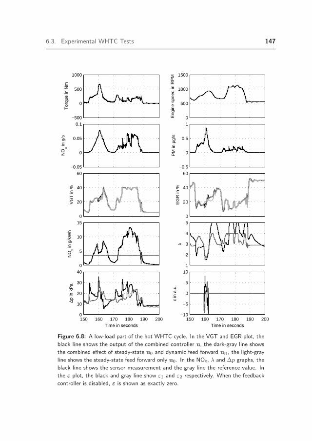
6.3. Experimental WHTC Tests 147
−500
0
500
1000
Tor
que
in N
m
0
500
1000
1500
Eng
ine
spee
d in
RP
M−0.05
0
0.05
0.1
NO
x in g
/s
−0.5
0
0.5
1
PM
in µ
g/s
0
20
40
60
VG
T in
%
0
20
40
60E
GR
in %
0
5
10
15
NO
x in g
/kW
h
1
2
3
4
5
λ
150 160 170 180 190 2000
10
20
30
40
∆p in
kP
a
Time in seconds150 160 170 180 190 200
−10
−5
0
5
10
ε in
a.u
.
Time in seconds
Figure 6.8: A low-load part of the hot WHTC cycle. In the VGT and EGR plot, theblack line shows the output of the combined controller u, the dark-gray line showsthe combined effect of steady-state u0 and dynamic feed forward uff , the light-grayline shows the steady-state feed forward only u0. In the NOx, λ and ∆p graphs, theblack line shows the sensor measurement and the gray line the reference value. Inthe ε plot, the black and gray line show ε1 and ε2 respectively. When the feedbackcontroller is disabled, ε is shown as exactly zero.
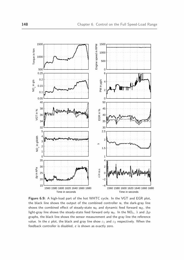
148 Chapter 6. Control on the Full Speed-Load Range
500
1000
1500
Tor
que
in N
m
0
500
1000
1500
Eng
ine
spee
d in
RP
M0.05
0.1
0.15
0.2
0.25
NO
x in g
/s
0
2
4
6
PM
in µ
g/s
32
34
36
38
40
VG
T in
%
30
35
40
45
50E
GR
in %
0
1
2
3
4
5
NO
x in g
/kW
h
1
1.5
2
2.5
λ
1560 1580 1600 1620 1640 1660 168015
20
25
30
35
∆p in
kP
a
Time in seconds1560 1580 1600 1620 1640 1660 1680
−4
−2
0
2
4
ε in
a.u
.
Time in seconds
Figure 6.9: A high-load part of the hot WHTC cycle. In the VGT and EGR plot,the black line shows the output of the combined controller u, the dark-gray lineshows the combined effect of steady-state u0 and dynamic feed forward uff , thelight-gray line shows the steady-state feed forward only u0. In the NOx, λ and ∆pgraphs, the black line shows the sensor measurement and the gray line the referencevalue. In the ε plot, the black and gray line show ε1 and ε2 respectively. When thefeedback controller is disabled, ε is shown as exactly zero.
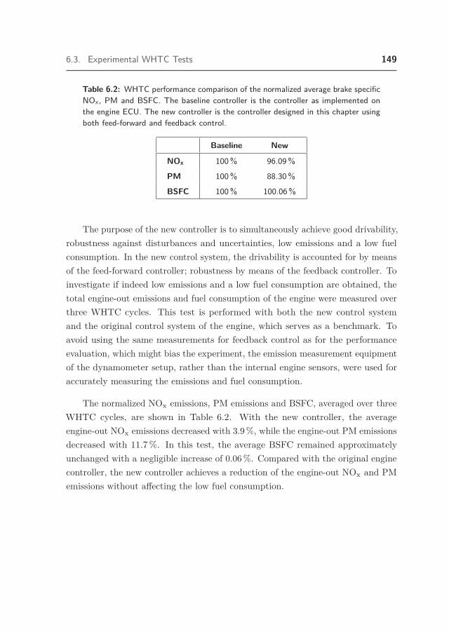
6.3. Experimental WHTC Tests 149
Table 6.2: WHTC performance comparison of the normalized average brake specificNOx, PM and BSFC. The baseline controller is the controller as implemented onthe engine ECU. The new controller is the controller designed in this chapter usingboth feed-forward and feedback control.
Baseline New
NOx 100% 96.09%
PM 100% 88.30%
BSFC 100% 100.06%
The purpose of the new controller is to simultaneously achieve good drivability,robustness against disturbances and uncertainties, low emissions and a low fuelconsumption. In the new control system, the drivability is accounted for by meansof the feed-forward controller; robustness by means of the feedback controller. Toinvestigate if indeed low emissions and a low fuel consumption are obtained, thetotal engine-out emissions and fuel consumption of the engine were measured overthree WHTC cycles. This test is performed with both the new control systemand the original control system of the engine, which serves as a benchmark. Toavoid using the same measurements for feedback control as for the performanceevaluation, which might bias the experiment, the emission measurement equipmentof the dynamometer setup, rather than the internal engine sensors, were used foraccurately measuring the emissions and fuel consumption.
The normalized NOx emissions, PM emissions and BSFC, averaged over threeWHTC cycles, are shown in Table 6.2. With the new controller, the averageengine-out NOx emissions decreased with 3.9%, while the engine-out PM emissionsdecreased with 11.7%. In this test, the average BSFC remained approximatelyunchanged with a negligible increase of 0.06%. Compared with the original enginecontroller, the new controller achieves a reduction of the engine-out NOx and PMemissions without affecting the low fuel consumption.


7 Conclusions &Recommendations
151
7.1 Conclusions
In this thesis, the design of a control system for the air path of a EURO VIheavy-duty diesel engine is elaborated, which uses the Variable Geometry Turbine(VGT) and Exhaust Gas Recirculation (EGR) valve as actuators. Compared withalternative methods for air-path control design, the work in this thesis focusses inparticular on reducing the effects of disturbances on the engine-out emissions andfuel efficiency, and on reducing the control design effort.
7.1.1 Disturbance Rejection
Reducing the effects of disturbances has gained great importance with the introduc-tion of the in-service conformity limits in the EURO VI legislation. This legislationimposes emission limits for real-life usage of diesel powered vehicles. Because vary-ing external conditions, ageing and production tolerances all affect the producedemissions, a control strategy that reduces the effects of these disturbances is neededto guarantee compliance with the new legislation.
In this thesis, a new method for disturbance rejection is elaborated. A newselection of controlled outputs is proposed: the engine-out NOx emissions, theair-fuel equivalence ratio (λ), and the pressure difference between the intake andexhaust manifold (∆p). These outputs are selected for their direct relation with thehigh-level objectives: NOx emissions, PM emissions and fuel efficiency, respectively,which is beneficial for the effectiveness of the feedback controller.

152 Chapter 7. Conclusions & Recommendations
The addition of ∆p as a controlled output is particularly important for therobustness. It is shown that control of NOx and λ only, using the VGT and EGRvalve, constitutes an ill-conditioned control problem. With the addition of ∆p, awell-conditioned control problem can be constituted. Moreover, with control of ∆p,the effect of disturbances on the fuel efficiency is reduced, and in addition the effectof control actions for disturbance rejection on NOx and λ on the fuel efficiency isreduced. For heavy-duty diesel engines, the fuel efficiency is very important, andwith the anticipated fuel efficiency legislation, its importance will further increase.
Via Singular Value Decomposition (SVD) decoupling, the two-input three-output configuration is converted into a decoupled two-input two-output system.For this system, a diagonal PI controller is designed using loopshaping. Thecontroller is tested in simulation and experiments. In simulation, its effectivenessat reducing the effects of disturbances is shown. With the controller enabled, thedeteriorating effect of the disturbances on the average NOx and PM emissions andfuel consumption is neutralized and the variation of the NOx and PM emissions,and ∆p is reduced by an order of magnitude. In experiments, the effectivenessof the controller for disturbance rejection and its functioning over the operatingrange of the engine are shown.
7.1.2 Design Effort
The control design effort for diesel engines is a bottleneck in the overall enginedesign. With new generations of diesel engines, the number of sensors and actuatorsincreased. This enlarged the potential for performance improvements by means ofcontrol, but a simultaneous increase in control design effort is observed. Takinginto account the control design effort, when designing control techniques for dieselengines, is therefore increasingly relevant.
In this thesis, three measures are taken to reduce the control design effort.
• Use feedback control for disturbance rejection. With an effective feedbackcontroller, the effects of disturbances are diminished. The need for enginemaps that compensate for disturbances is thereby reduced. This reducesthe number of parameters that require calibration, and thereby reduces thecontrol design effort.

7.1. Conclusions 153
• Use a systematic, offline control design. A design path is followed thatconsists of: model identification, control design, and performance evaluation.A time-efficient and accurate procedure for modeling the engine behavior isexperimentally applied and extensively analyzed. The identified FRF modelscharacterize the dynamic input-output behavior of the engine. The designof the feedback controller is based entirely on these FRF models. This way,the controller is designed such that it works well in conjunction with theinput-output behavior of the engine, without the time-consuming process ofmanually adapting the controller parameters and empirically determining itseffect on the engine performance. After control design, the performance isexperimentally evaluated to determine if indeed the expected performancelevel is realized.
• Use low-complexity control elements. A range of control design techniques(see Chapter 3) is suitable to fulfill the above two requirements. The proposedcontrol design consists of PI control and SVD decoupling. Compared withthe alternatives, this has the advantage that the complexity of the controllerand its design process is low. Various alternative methods for linear controldesign are used in literature, but these require some form of gain-schedulingto work on the entire operating range. By focussing on robustness in thesystem layout, scheduling of the control parameters is not required. An LTIfeed-forward controller combined with a PI controller with static decouplingmatrices, both with fixed parameters, is sufficient to control the engine overits entire operating range.
7.1.3 Summary of the Main Results
The control design process, as elaborated in this thesis, is divided into systemidentification, disturbance rejection around a fixed operating point, and controlover the full operating range. The main conclusions resulting from these parts areseparately addressed in the following.
Identification
In Chapter 4, a method for identification of the sensor response to variationsin the actuators, i.e., the input-output response, is elaborated. For this, thelocal Frequency Response Function (FRF) at a fixed speed-load operating point is

154 Chapter 7. Conclusions & Recommendations
measured using multisine excitation. Compared with alternative modeling methods,the ability to include any measured output in the model, without complicating themodeling procedure, is an advantage. Also, the natural inclusion of sensor andactuator dynamics into the model is an advantage for the application of controldesign. The considered actuators are the VGT and EGR valve, the measurementsare the engine-out NOx emissions, air-fuel equivalence ratio and pressure differencebetween the intake and exhaust manifold. It is found that using only ten minutesof identification data, the local input-output behavior can be captured accurately.The effects of noise and nonlinearity on the local engine behavior are individuallyquantified and it is shown that these effects are an order of magnitude smaller thanthe linear effects. Using the linear FRF models, the actual engine measurementsin a single speed-load point are reconstructed with average squared errors smallerthan 3% of the actual response.
Disturbance Rejection
Chapter 5 discusses control design to reduce the effects of disturbances. The goal ofthe controller is to keep the engine-out emissions of NOx, PM and the fuel efficiencyclose to their respective nominal values, despite the effects of external influences.To realize this, a feedback controller is designed. A new selection of controlledoutputs is made: NOx, λ and ∆p. These outputs are selected because they reflectthe engine-out NOx emissions, PM emissions and fuel efficiency, respectively. Withtwo actuators and three measured outputs, the resulting input-output system isunderactuated. It is argued that the expected Pareto-optimality of the combinationof NOx, PM and fuel efficiency implies that regardless of the number of actuators,only two controllable directions are available. This means that the underactuationdoes not induce an additional limitation. Using SVD-decoupling and loopshaping,a feedback controller is designed to control the underactuated input-output system.In a simulation, where disturbances are applied in the inputs, operating point andambient conditions, the controller is shown to reduce the variation of the NOx andPM emissions and ∆p with a factor 12, 5 and 14, respectively. In addition, theincrease of the average emissions and fuel efficiency is neutralized, resulting in areduction of the average NOx and PM emissions with 14% and 19%, respectively,and a reduction of 0.74% of the BSFC. The controller is also tested experimentally,while step disturbances are applied in the inputs and the engine speed and load. Itis again shown that the feedback controller maintains the tradeoff between NOx,

7.1. Conclusions 155
λ and ∆p and reduces the effects of the applied disturbances on the individualoutputs.
Full Operating Range
In Chapter 6, an air-path control system is designed that can be used on the fullengine speed-load range and features a particularly low design effort. The identi-fication method of Chapter 4 is used to efficiently model the local input-outputbehavior in a grid of operating points covering the full speed-load range. The feed-back control design of Chapter 5 is reused and modified to accommodate differentengine speeds and loads. An additional dynamic feed-forward controller is designedto reduce the PM emissions and improve the torque response during tip-in torquetransients. This feed-forward controller is calibrated manually on a dynamometersetup. This enables the evaluation of the transient NOx emissions, PM emissionsand torque response during calibration. Both the feedback controller and thefeed-forward controller are of low-order LTI form and do not require scheduling oftheir parameters. Therefore, they have a particularly low design complexity andimplementation footprint. The combined controller is experimentally tested on theWorld Harmonized Transient Cycle (WHTC). Compared with the controller origi-nally implemented on the engine ECU, the emissions over the WHTC of both NOx
and PM are reduced with 3.9% and 11.7%, respectively. The fuel consumptionover the WHTC remained approximately unchanged.
Summarising, a control design procedure for air-path control of clean dieselengines was formulated. The design procedure comprises system identification, afeedback controller for disturbance rejection and a feed-forward controller for im-proved transient performance. The designed controller is tested both in simulationand experimentally on a modern EURO VI engine. It is shown that due to thefeedback controller, the performance of the engine remains close to the nominalperformance when disturbances are applied. On WHTC experiments, it is shownthat with the newly designed controller, the NOx and PM emissions are reduced,compared with the original controller. The presented control design procedure istime efficient and the resulting controller has a small implementation footprint.

156 Chapter 7. Conclusions & Recommendations
7.2 Recommendations for Future Research
The current work presents a proof of concept for a new diesel engine controldesign using the air-path actuators. Several potential improvements to the controldesign framework can be considered and are outlined below. First, adaptations toimprove on the limitations of the proposed control design are addressed. Becausethe applied modeling procedure is also useful outside of the proposed control designframework, recommendations for adapting the modeling procedure are addressedseparately. When reconsidering the use of air path control in the overall enginecontrol problem, including the aftertreatment system, further opportunities forimprovement are discerned, which are discussed at the end of this section.
7.2.1 Improved Air Path Control
Control Algorithm
The current control design has a low design effort. When the process of optimizingthe steady-state engine performance is completed; and assuming that the necessarypreparations to process and evaluate the data are made and an I/O-board tointerface with the engine is available. Identification and design of the feedback andfeed-forward controller can optimistically be completed in a single day.
The choice to minimize complexity, rather than to maximize the performanceinduces a performance penalty. To quantify to what extent this affects the emissionsand fuel consumption, a comparison with a less conservative control design shouldbe made. For example, a gain-scheduled H∞ controller can replace the currentfeedback controller and serve as a high-performance benchmark. This removes theconservatism introduced by the decoupling and linear PI control design and adaptsthe control behavior to the local engine behavior. Depending on the achievedperformance increase, an increase in the controller complexity may be justifiedand a more complex control design can be considered. The gain-scheduled H∞controller is likely too complex to implement in production. But implementing,e.g., scheduling of the PI parameters requires only a moderate increase in thecontroller complexity and design effort. Similarly, scheduling can also be appliedto the parameters of the feed-forward controller, e.g., based on the engine speed.The added flexibility can be used to control the emission tradeoff more closely.
7.2. Recommendations for Future Research 157
Controlled Outputs
The BSFC, NOx and PM are considered the main performance measures thatrequire feedback control. To increase the effectiveness of the feedback controllerwith regards to disturbance rejection on these measures, the use of alternativesensors that more directly reflect these measures can be considered.
When a PM sensor becomes available, direct control of measured PM emissionsis possible. This enables more direct control of the emissions and more tightcompliance with the emission legislation. The use of λ instead of PM, as used inthis thesis, also has advantages. The λ output is also a relevant measure for theengine’s ability to quickly respond to an increase in torque demand. Controlling λ,rather than PM, is therefore beneficial for maintaining the desired torque responsewhen disturbances affect the engine. It is therefore not obvious whether controllingPM, rather than λ, improves the engine performance.
When the in-cylinder pressure is measured, a number of different controlapplications become possible. The fast dynamic response of the in-cylinder mea-surements is well suited to be combined with the fast actuators in the fuel path.Some examples that become possible are: control of the combustion timing viathe injection timing; control of the combustion profile via the injection profile;and control of IMEP via the injection quantity. Also, the indicated specific fuelconsumption can be determined using the in-cylinder pressure. This informationcan be used to further improve the air-path controller. In the control design inthis thesis, only the PMEP effect on the BSFC is used for disturbance rejection.This can be complemented with the IMEP effect, when the in-cylinder pressure ismeasured. This enables more direct control of the BSFC.
With the current control design, the sensor dynamics of the NOx sensor area bottleneck for the achieved closed-loop bandwidth. This limitation can besurmounted either by using a sensor that does not suffer as much from sensordynamics (Karlsson et al., 2010) or by using an additional observer (Tschanz et al.,2013). When the limitations of sensor dynamics are removed, the internal air-pathdynamics limit the closed-loop bandwidth. This enables the design of a feedbackcontroller that achieves faster disturbance rejection.
158 Chapter 7. Conclusions & Recommendations
Experiments
Further testing of the controller in more realistic scenarios is advised to determineif the controller and disturbance rejection remain effective in real-world scenarios.When a series of engines is tested, the effects of production tolerances on theengine performance, and the effectiveness of the feedback controller on reducing theperformance differences can be quantified. Similarly, engines of a different age andmaintenance state, and the effects of fuel quality, ambient temperature, pressureand humidity should be tested. The presented simulation results in Chapter 5indicate that the controller can be expected to handle these disturbances well. Anexperimental validation is, however, much more convincing.
Transients
The engine performance during fast operating-point transients is not well reflectedin the design of the feedback controller. The proposed sensor layout and feedbackbandwidth are designed to reduce the effects of slowly varying disturbances andmaintain close to optimal performance in steady state. Ideally, a feedback controllershould improve the transient performance as well as achieve disturbance rejection.
The time scales relevant for evaluating emissions and fuel consumption aremuch longer than those for evaluating performance during an operating pointtransient. A temporary 20% difference between the nominal emissions and theactual emissions during a tip-in transient can well be tolerated if this averagesout over time. Nonetheless feedback control can also be relevant for improvingthe performance during fast transients. When, during transients, a feedbackcontroller assists in controlling, e.g., the fresh air flow, turbine speed or both,the transient engine response can become less sensitive to how well the feed-forward characteristics match the actual engine characteristics. This can reducethe calibration effort needed for improving torque transients and reduce the effectsof disturbances on the torque response.
7.2. Recommendations for Future Research 159
7.2.2 Modeling
The presented modeling procedure is both accurate and fast for the considereduse case and is suitable for the proposed control design. A further improvementof the accuracy or a reduction of the required identification effort will thereforenot significantly improve the overall modeling process. The range of applicationsfor which the resulting models can be used with high accuracy is however ratherlimited. A modified identification procedure that results in more versatile models,that are suitable for more applications, would be an improvement. Additionalapplications that can be considered are described below. The challenge whenadapting the modeling procedure is to maintain the strong features of the currentmodeling procedure, i.e., the high and quantifiable accuracy, ability to modelany input-output combination and the inclusion of sensor and actuator dynamics.Recommendations for changes to the modeling procedure that can be consideredare discussed next.
The number of actuators that are considered can be extended. When inaddition to the excitations in the VGT and EGR valve, also excitations in theengine speed or fuel quantity are applied, these effects can be modeled as well. Thiscan be useful, e.g., for calculating control actions during operating point changes.When the use of, e.g., the SOI or BPV for feedback control is considered, anexcitation signal can be added here as well. Adding excitation signals to additionalactuators does come at the expense of either the identification accuracy or therequired identification time. Additional outputs, e.g., the mass air flow or exhausttemperature, can be modeled without modifying the identification experimentand without compromising the identification accuracy or identification time. Thefrequency response of any sensor signal that was measured during the identificationexperiment can be determined the using analysis procedure in Chapter 4.
The conversion of the FRF into a different model type can also make themodels more suitable for (quasi) linear model-based control design, which is usedin most of the control design methods described in Chapter 3. A conversion of theFRF into to a different model type, such as a linear state-space model makes themodels more suitable to be used for this.
For simulating drive cycles, large speed and load transients must be consideredand included in the modeling process. During these transients, the effects of
160 Chapter 7. Conclusions & Recommendations
nonlinear behavior can be expected to become dominant over the linear behavior.Significant changes to both the modeling and identification process are requiredto accurately capture this. A different model structure should be selected, suchthat the nonlinear behavior can be modeled accurately. Also, the identificationexperiment should be changed. The current experiment was designed to accuratelyidentify the local input-output response. By maintaining close to a fixed operatingpoint, the effects of operating point variations are excluded from the experimentalresults as much as possible. Therefore, the current experiment is not suitablefor identifying the dynamic effects of operating point variations. In literature,mean-value models, which are based on approximate physical relations, are oftenused for simulating drive cycles. These models are more suitable for this purpose.Compared with the FRF models, the local accuracy and the ability to easily includeany available input-output combination in the model are compromised.
7.2.3 Integrated Engine Control
A further synergy between the control system of the air path and the aftertreatmentsystem presents opportunities for improvements in two ways. First, control of theair path can be used to increase the conversion efficiency of the SCR system.Second, the state of the SCR system can be used to dynamically schedule theallowed engine-out emissions. This is explained below in more detail.
The exhaust gas temperature, which is affected by the VGT an EGR valve,affects the conversion efficiency of NOx in SCR catalysts. When the exhaust gastemperature is controlled to be at its optimal level for NOx conversion, increasedengine-out NOx emissions can be allowed, without increasing the tailpipe-outemissions. This presents an opportunity to further reduce the PM emissions andBSFC. It is worth noting that an increased exhaust gas temperature also impliesan increase of the BSFC. It is therefore not a priory clear if the allowed increasein engine-out NOx also results in a reduced BSFC.
When the conversion efficiency of the SCR catalyst is known, this informationcan be used to dynamically schedule the allowed engine-out NOx emissions. Whenthe conversion efficiency is high, increased engine-out NOx emissions can be allowed,without increasing the tailpipe-out emissions. The allowed increase in engine-outemissions can be used to further optimize the fuel efficiency. In Willems et al. (2013),

7.2. Recommendations for Future Research 161
the potential to reduce the fuel consumption using this method is experimentallydemonstrated.


Bibliography
163
ACEA. Commercial vehicles and CO2. Technical report, ACEA, 2010.
D. Alberer and L. Del Re. Optimization of the transient diesel engine operation.Proceedings of the 9th International Conference on Engines and Vehicles, Capri,Naples, Italy, SAE Technical Paper 2009-24-0113, 2009.
D. Alberer and L. Del Re. On-line abatement of transient NOx and PM dieselengine emissions by oxygen based optimal control. SAE paper 2010-01-2201, 102010.
D. Alberer, H. Hjalmarsson, and L. Del Re. System identification for automotivesystems: Opportunities and challenges. In D. Alberer, H. Hjalmarsson, andL. Del Re, editors, Identification for Automotive Systems, volume 418 of LectureNotes in Control and Information Sciences, pages 1–10. Springer London, 2012.
E. Alfieri. Emissions-controlled diesel engine. PhD thesis, ETH Zurich, Switzerland,2009.
M. Benz. Model-based optimal emission control of diesel engines. PhD thesis, ETHZurich, Switzerland, 2010.
A. Brahma. Methodologies for Modeling and Feedback Control of the NOx-BSFCTrade-Off in High-Speed, Common-Rail, Direct-Injection Diesel Engines. PhDthesis, The Ohio State University, USA, 2005.
J. Chauvin, G. Corde, N. Petit, and P. Rouchon. Motion planning for experimentalairpath control of a diesel homogeneous charge-compression ignition engine.Control Engineering Practice, 16(9):1081–1091, 2008.

164
C. Criens, F. Willems, T. van Keulen, and M. Steinbuch. Experimental controldesign for robust low emission, fuel efficient diesel engines. Submitted for JournalPublication, 2014.
C. Criens, T. van Keulen, F. Willems, and M. Steinbuch. A control orientedmultivariable identification procedure for turbocharged diesel engines. Submittedfor journal publication, 2013a.
C. Criens, F. Willems, and M. Steinbuch. Under actuated air path control of dieselengines for low emissions and high efficiency. In Proceedings of the FISITA 2012World Automotive Congress, pages 725–737. Springer, 2013b.
H. Dekker and W. Sturm. Simulation and control of a HD diesel engine equippedwith new EGR technology. SAE Technical Paper 960871, 1996.
L. Del Re, P. Ortner, and D. Alberer. Modeling alternatives for automotivepredictive control. In Proceedings of the ECOSM09, 2009.
DieselNet. Emission standards, European Union, heavy-duty truck and bus engines,2013. URL http://www.dieselnet.com/standards/.
T. Dobrowiecki and J. Schoukens. Linear approximation of weakly nonlinearmimo systems. Instrumentation and Measurement, IEEE Transactions on, 56(3):887–894, 2007.
European Commission. Commission regulation (EU) No 582/2011 of 25 May2011 implementing and amending regulation (EC) No 595/2009 of the Europeanparliament and of the council with respect to emissions from heavy duty vehi-cles (Euro VI) and amending annexes I and III to directive 2007/46/ec of theEuropean parliament and of the council text with EEA relevance, May 2011.
European Environment Agency. European union emission inventory report 1990-2011 under the UNECE convention on long-range transboundary air pollution(lrtap). Technical Report 10/2013, European Union, 2013.
H. J. Ferreau, P. Ortner, P. Langthaler, L. Del Re, and M. Diehl. Predictive controlof a real-world diesel engine using an extended online active set strategy. AnnualReviews in Control, 31(2):293–301, 2007.

165
S. García-Nieto, M. Martínez, X. Blasco, and J. Sanchis. Nonlinear predictivecontrol based on local model networks for air management in diesel engines.Control Engineering Practice, 16(12):1399–1413, 2008.
N. Gense, C. Such, and L. Ntyiachristos. Euro VI technologies and costs for heavyduty vehicles. TNO Science and Industry report, 6(06.OR.PT.023.2/NG), 2006.
M. Grahn, K. Johansson, and T. McKelvey. A diesel engine management systemstrategy for transient engine operation. In 7th IFAC Symposium on Advancesin Automotive Control, pages 1–6, 2013.
C. Guardiola, A. Gil, B. Pla, and P. Piqueras. Representation limits of meanvalue engine models. In D. Alberer, H. Hjalmarsson, and L. Del Re, editors,Identification for Automotive Systems, chapter 11, pages 185–206. Springer Berlin/ Heidelberg, 2012.
L. Guzzella and A. Amstutz. Control of diesel engines. Control Systems, IEEE,18(5):53–71, 1998.
L. Guzzella and C. Onder. Introduction to modeling and control of internal com-bustion engine systems. Springer, 1 edition, 2004.
M. Henningsson. Data-Rich Multivariable Control of Heavy-Duty Engines. PhDthesis, Department of Automatic Control, Lund University, Sweden, 2012.
M. Henningsson, K. Ekholm, P. Strandh, P. Tunestål, and R. Johansson. Dy-namic mapping of diesel engine through system identification. In D. Alberer,H. Hjalmarsson, and L. Del Re, editors, Identification for Automotive Systems,chapter 13, pages 223–240. Springer, 2012.
M. Herceg, T. Raff, R. Findeisen, and F. Allgowe. Nonlinear model predictivecontrol of a turbocharged diesel engine. In Computer Aided Control SystemDesign, 2006 IEEE International Conference on Control Applications, 2006IEEE International Symposium on Intelligent Control, 2006 IEEE, pages 2766–2771, 2006.

166
M. Hirsch, K. Oppenauer, and L. Del Re. Dynamic engine emission models. InL. Del Re, F. Allgöwer, L. Glielmo, C. Guardiola, and I. Kolmanovsky, editors,Automotive Model Predictive Control, chapter 5, pages 73–87. Springer Berlin /Heidelberg, 2010.
M. Jankovic, M. Jankovic, and I. Kolmanovsky. Constructive Lyapunov controldesign for turbocharged diesel engines. Control Systems Technology, IEEETransactions on, 8(2):288–299, 2000.
M. Jung and K. Glover. Calibratable linear parameter-varying control of a tur-bocharged diesel engine. Control Systems Technology, IEEE Transactions on,14(1):45–62, 2006.
M. Karlsson, K. Ekholm, P. Strandh, R. Johansson, and P. Tunestal. Multiple-inputmultiple-output model predictive control of a diesel engine. In Proceedings ofthe Sixth IFAC Symposium in Automotive Control, Munich, Germany, volume 1,pages 124–129, 2010.
T. Koji and Y. Kazuhiro. A study on the cell structure and the performances ofwall-flow diesel particulate filter. Energy, 48(1):492–499, 2012.
I. Kolmanovsky, P. Moraal, M. Van Nieuwstadt, and A. Stefanopoulou. Issues inmodelling and control of intake flow in variable geometry turbocharged engines.Chapman and Hall CRC research notes in mathematics, pages 436–445, 1999.
T. Körfer, L. Ruhkamp, O. E. Herrmann, R. Linssen, and D. Adolph. Verschärfteanforderungen an die luftpfadregelung bei nutzfahrzeug-motoren. MTZ - Mo-tortechnische Zeitschrift, 69(11):958–965, 2008.
L. Ljung. System identification, Theory for the User. Wiley Online Library, 2edition, 1999.
M. Mrosek, H. Sequenz, and R. Isermann. Identification of emission measurementdynamics for diesel engines. In 18th IFAC World Congress, Italy, pages 11839–11844, 2011.
M. van Nieuwstadt, I. Kolmanovsky, P. Moraal, A. Stefanopoulou, and M. Jankovic.EGR-VGT control schemes: experimental comparison for a high-speed dieselengine. Control Systems, IEEE, 20(3):63–79, 2000.

167
P. Ortner and L. Del Re. Predictive control of a diesel engine air path. ControlSystems Technology, IEEE Transactions on, 15(3):449–456, 2007.
P. Ortner, R. Bergmann, H. Ferreau, and L. Del Re. Nonlinear model predictivecontrol of a diesel engine airpath. In IFAC Workshop on Control Applicationsof Optimisation, Jyvaskyla, pages 91–96, 2009.
D. Pachner, D. Germann, and G. Stewart. Identification techniques for controloriented models of internal combustion engines. In D. Alberer, H. Hjalmarsson,and L. Del Re, editors, Identification for Automotive Systems, chapter 15, pages257–282. Springer, 2012.
R. Pintelon and J. Schoukens. System identification: a frequency domain approach.Wiley-IEEE Press, 1 edition, 2001.
D. Rijlaarsdam, B. van Loon, P. Nuij, and M. Steinbuch. Nonlinearities in industrialmotion stages - detection and classification. In American Control Conference,2010, pages 6644–6649, 2010.
J. Schoukens, R. Pintelon, T. Dobrowiecki, and Y. Rolain. Identification of linearsystems with nonlinear distortions. Automatica, 41(3):491–504, 2005.
H. Sequenz, M. Mrosek, S. Zydek, and R. Isermann. Model based optimisationof a step in acceleration for a CR-diesel engine. In World Congress, volume 18,pages 13016–13021, 2011.
X. Seykens. Engine simulation tool DYNAMO. Technical report, TNO Automotive,2009.
X. Seykens. Development and validation of a phenomenological diesel engine com-bustion model. PhD thesis, Eindhoven University of Technology, The Netherlands,2010.
S. Skogestad and I. Postlethwaite. Multivariable feedback control: analysis anddesign, volume 2. Wiley, 2007.
I. Stamati, D. Telen, F. Logist, E. Van Derlinden, M. Hirsch, T. Passenbrunner, andJ. Van Impe. Optimal experimental design for mechanistic nonlinear dynamicmodels using multisine inputs: Application to a diesel engine. In AmericanControl Conference, 2012, pages 4227–4232, 2012.

168
A. Stefanopoulou, I. Kolmanovsky, and J. Freudenberg. Control of variable ge-ometry turbocharged diesel engines for reduced emissions. Control SystemsTechnology, IEEE Transactions on, 8(4):733–745, 2000.
G. Stewart, F. Borrelli, J. Pekar, D. Germann, D. Pachner, and D. Kihas. Towarda systematic design for turbocharged engine control. In L. Del Re, F. Allgöwer,L. Glielmo, C. Guardiola, and I. Kolmanovsky, editors, Automotive Model Pre-dictive Control, chapter 14, pages 211–230. Springer Berlin / Heidelberg, 2010.
T. Tienstra. Optimization of tip-in transients for a heavy duty diesel engine.Masters Thesis CST 2013.045, Eindhoven University of Technology, 2013.
F. Tschanz, A. Amstutz, C. Onder, and L. Guzzella. Feedback control of particulatematter and nitrogen oxide emissions in diesel engines. Control EngineeringPractice, 21(12):1809–1820, 2013.
R. Van Helden, R. Verbeek, F. Willems, and R. van der Welle. Optimization ofurea SCR deNOx systems for HD diesel engines. SAE Technical Paper, 1(SAE2004-01-0154), 2004.
K. Vanhoenacker, T. Dobrowiecki, and J. Schoukens. Design of multisine ex-citations to characterize the nonlinear distortions during FRF-measurements.Instrumentation and Measurement, IEEE Transactions on, 50(5):1097–1102,2001.
A. S. Verma. Airpath modelling of turbocharged diesel engine in transient operationand investigation. International Journal of Advanced Technology and EngineeringResearch, 3(1):1–10, 2013.
J. Wahlström. Control of EGR and VGT for emission control and pumping workminimization in diesel engines. PhD thesis, Department of Electrical Engineering,Linköpings universitet, 2009.
J. Wahlström and L. Eriksson. Robust nonlinear EGR and VGT control withintegral action for diesel engines. In 17th IFAC World Congress, Korea, 2008.
J. Wahlstrom and L. Eriksson. Output selection and its implications for MPC ofEGR and VGT in diesel engines. Control Systems Technology, IEEE Transactionson, 21(3):932–940, 2013.

169
J. Wahlström, L. Eriksson, and L. Nielsen. EGR-VGT control and tuning forpumping work minimization and emission control. Control Systems Technology,IEEE Transactions on, 18(4):993–1003, 2010. ISSN 1063-6536.
J. Wahlström and L. Eriksson. Modelling diesel engines with a variable-geometryturbocharger and exhaust gas recirculation by optimization of model parametersfor capturing non-linear system dynamics. Proceedings of the Institution ofMechanical Engineers, Part D: Journal of Automobile Engineering, 225(7):960–986, 2011.
X. Wang, H. Waschl, D. Alberer, and L. Del Re. A design framework for predic-tive engine control. Oil & Gas Science and Technology–Revue d’IFP Energiesnouvelles, 66(4):599–612, 2011.
H. Waschl, D. Alberer, A. Kerschbaummayr, and L. Del Re. Reliable referencedetermination for diesel engine emission control. In American Control Conference,2012, pages 4215–4220, 2012.
X. Wei and L. Del Re. Gain scheduled H∞ control for air path systems of dieselengines using LPV techniques. Control Systems Technology, IEEE Transactionson, 15(3):406–415, 2007.
F. Willems and R. Cloudt. Experimental demonstration of a new model-basedSCR control strategy for cleaner heavy-duty diesel engines. Control SystemsTechnology, IEEE Transactions on, 19(5):1305–1313, 2011.
F. Willems, P. Mentink, F. Kupper, and E. van den Eijnden. Integrated emissionmanagement for cost optimal EGR-SCR balancing in diesels. In 7th IFACSymposium on Advances in Automotive Control, pages 701–706. Japan : IFAC,September 2013.
D. Zhao, C. Liu, R. Stobart, J. Deng, E. Winward, and G. Dong. An explicitmodel predictive control framework for turbocharged diesel engines. IndustrialElectronics, IEEE Transactions on, PP(99):1–1, 2013.


Summary
171
Air-Path Control of Clean Diesel Enginesfor disturbance rejection on NOx, PM and fuel efficiency
This thesis deals with the design of a control system for heavy-duty dieselengines, which makes use of the Variable Geometry Turbine (VGT) and ExhaustGas Recirculation (EGR) valve. The goal of this control system is to simultaneouslyachieve a low fuel consumption and low engine-out NOx and PM emissions, andto maintain these properties when disturbances are present. In addition, a controldesign method with a low design effort and complexity is aimed for.
The new EURO VI emission legislation for heavy-duty diesel engines requiresa reduction of the Nitrogen Oxides (NOx) and Particulate Matter (PM) emissionsof 80% and 50%, respectively, compared with the EURO V legislation. Moreover,it requires that these low emissions are achieved under real-world conditions, whichimplies that the effects of, e.g., production tolerances, ageing and changing ambientconditions have to be accounted for. This can in part be achieved via improvedcontrol using the VGT and EGR valve. A VGT can adapt the flow area of theturbine, which influences the power generated by the turbine as well as the flowthrough the turbine. The EGR system is used to dilute the intake air with cooledexhaust gas. This reduces the temperatures reached during combustion, whichreduces the NOx emissions. The EGR flow is throttled by a controllable EGRvalve, such that a favorable balance between the positive effects (reduced NOx
emissions) and the negative effects (increased PM emissions, decreased combustionefficiency, increased pumping work) of EGR can be maintained. Combined, the

172
VGT and EGR valve determine the pressures and flows in the air path and therebythey influence the emissions and fuel efficiency.
The control design process, which is elaborated in this thesis, can be dividedinto three parts: system identification, disturbance rejection around a fixed operat-ing point, and control over the full speed-load range of the engine. In the following,these parts are individually addressed.
Multisine Frequency Response Function (FRF) identification is used as anaccurate and time-efficient method for modeling the input-output dynamics at afixed engine speed-load point. The considered inputs are the VGT and EGR valve;the considered outputs are the engine-out NOx emissions, the air-fuel equivalenceratio, and the pressure difference between the intake and exhaust manifold. Theresulting model accuracy is extensively analyzed. The effects of noise and nonlin-earities on the local system behavior and the distortion of the FRF as a result ofthese effects are separated and individually quantified as a function of frequency.It is found that with ten minutes of identification data, an accurate Multi-InputMulti-Output (MIMO) model of the local behavior in a single speed-load point isidentified. That is, the effects of the above mentioned distortions are an order ofmagnitude smaller than the modeled linear behavior. The identification procedureis used repeatedly to model the local behavior on a grid of engine speed-load pointsthat covers the full operating range of the engine. Large difference in the localbehavior at different speed-load points are identified that include variations in theinput-output gain of a full order of magnitude.
A feedback controller is designed, that is aimed at maintaining the brakespecific fuel consumption (BSFC), NOx emissions and PM emissions at all timesas close as possible to the values obtained under nominal conditions. It is foundthat for the performance of this feedback controller, the selection of the controlledoutputs is critical. Outputs that reflect the main performance measures: NOx, PMand BSFC, are preferable. For this reason, three outputs are selected as controlledoutputs: the engine-out NOx sensor measurement, air-fuel equivalence ratio (λ),and pressure difference between intake and exhaust manifold, respectively. UsingSVD-decoupling, the three-output system is reduced to a decoupled Two-In, Two-Out (TITO) system. A diagonal PI controller is designed to control this TITOsystem. It is shown in a simulation with various disturbances that, despite thesedisturbances, the engine with the controller can achieve near-nominal average

173
NOx and PM emissions and fuel efficiency. For comparison, the same simulationis repeated without feedback control. With feedback enabled, the average NOx
and PM emissions and fuel consumption are reduced with 14%, 19% and 0.74%,respectively. Moreover, the feedback controller reduced the variation as a result ofdisturbances of the NOx and PM emissions and pressure difference with a factor12, 5 and 14, respectively. The controller is also tested experimentally, while stepdisturbances in the inputs and engine speed and load are applied. Its effectivenessat reducing the effects of disturbances is again demonstrated.
To control the air path over the full engine speed-load range, the effects ofnonlinear behavior have to be accounted for. It is shown that despite the encoun-tered nonlinear behavior, a linear feedback controller of the same structure as usedfor local disturbance rejection and with fixed parameters can also be effective fordisturbance rejection in the full operating range; using a linear controller, asymp-totic stability and a sufficient closed-loop bandwidth are achieved. To improve thetorque response and decrease the PM emissions during tip-in torque transients, acomplementary feed-forward controller is designed. This controller accelerates theturbine response and increases the fresh air flow during tip-in transients. For thefeed-forward controller, a control design with a fixed structure and two tunableparameters is used for each actuator. The emission measurement equipment that isavailable at the dynamometer test setup is used to evaluate the engine performancewhile tuning the controller parameters. It is shown experimentally that a two-second torque response can be combined with acceptable NOx and PM emissions.The combination of the feedback and feed-forward controllers constitutes a controlsystem that satisfies the performance requirements and features the desired lowdesign effort.
The performance of the engine, using the new feedback and feed-forwardcontroller, is demonstrated experimentally on a modern six-cylinder, heavy-duty,EURO VI engine. On the hot World Harmonized Transient Cycle (WHTC), whichis part of the EURO VI approval tests, reduced NOx (-3.9%) and PM (-11.7%)emissions are obtained, while maintaining the low fuel consumption that is obtainedwith the original engine controller.


Samenvatting
175
Ontwerp van een Luchtpadregeling voor Schone Dieselmotorenvoor verstoringsonderdrukking op NOx, PM en brandstofverbruik
Het onderwerp van dit proefschrift is het ontwerp van een regelsysteem voordieselmotoren in vrachtauto’s. De regelaar maakt gebruik van de Variabele Geo-metrie Turbo (VGT) en uitlaatgasrecirculatieklep (EGR klep). Het doel van hetregelsysteem is om een laag brandstofverbruik te combineren met een lage uitstootvan NOx en PM (Particulate Matter, ofwel fijnstof) en bovendien deze eigenschap-pen te behouden als er verstoringen aanwezig zijn. Een tweede doelstelling voorhet nieuwe regelaarontwerp is dat het in korte tijd geïmplementeerd kan worden.
De nieuwe EURO VI emissiewetgeving voor vrachtauto dieselmotoren schrijfteen vermindering van de NOx en PM uitstoot voor van respectievelijk 80% en 50%,ten opzichte van het EURO V niveau. Daarbij wordt ook voorgeschreven dat dezelage uitstoot tijdens bedrijf gehaald moet worden, wat impliceert dat de invloedenvan bijvoorbeeld productieverschillen, veroudering en veranderingen in de atmosfe-rische condities meegenomen moeten worden. Een verbeterde aansturing van deVGT en EGR klep kan hier een bijdrage aan leveren. Een turbo die is uitgevoerdmet VGT kan de geometrie van de turbine inlaat aanpassen. Hiermee verandert destroming door de turbine en ook het door de turbine opgewekte vermogen. Middelshet EGR systeem wordt de aangezogen lucht verdund met gekoelde uitlaatgassen.Hierdoor loopt de temperatuur tijdens verbranding minder hoog op, waardoor deNOx uitstoot vermindert. De EGR stroom wordt beperkt door een regelbare EGRklep, zodat de balans tussen de positieve effecten (verminderde NOx uitstoot) ende negatieve effecten (verhoogde PM uitstoot, slechtere verbranding, toegenomen

176
pompverliezen) van EGR gunstig blijft. De instellingen voor de VGT en EGR klepbeïnvloeden zo de NOx en PM emissies en het brandstofverbruik van dieselmotoren.
Het ontwerpproces van de regelaar, zoals uitgewerkt in dit proefschrift, is indrie onderdelen op te splitsen: systeem identificatie, verstoringsonderdrukking rondeen vast werkpunt, en regelacties over het volledige werkgebied. Deze onderdelenzullen nu individueel besproken worden.
Frequentie Response Functies (FRF), gemeten door middel van multisinusidentificatie, worden gebruikt als een nauwkeurige en efficiënte methode om het dy-namisch gedrag van de motor rond een vast werkpunt te modelleren. De gebruiktesysteemingangen zijn de VGT en EGR klep; de gemodelleerde uitgangen de NOx
uitstoot, lucht-brandstof verhouding, en het drukverschil tussen het inlaat- en uit-laatspruitstuk. Het model bevat alle dynamica tussen ingang en uitgang, inclusiefsensor- en acuatordynamica. De verkregen modelnauwkeurigheid is uitgebreid gea-nalyseerd. De effecten van ruis en niet-lineariteiten op het lokale systeemgedrag ende vervorming van de gemeten FRF als gevolg van deze effecten worden onderschei-den en individueel gekwantificeerd als functie van de frequentie. Met een metingvan tien minuten kan een nauwkeurig Multi-Input Multi-Output (MIMO) modelvan het lokale systeemgedrag worden geïdentificeerd, waarmee wordt bedoeld datde effecten van de eerder genoemde verstoringen minstens één orde grootte kleinerzijn dan het gemodelleerde lineaire gedrag. De identificatie procedure is meermaalstoegepast om zo het lokale systeemgedrag op een raster van werkpunten te modelle-ren. Grote onderlinge verschillen tussen het lokale systeemgedrag bij verschillendemotortoerentallen of verschillende koppels worden gevonden, waaronder een ordegrootte verschil in de magnitude van de FRF.
Er is een feedback regelaar ontworpen met het doel het brandstofverbruik ende uitstoot van NOx en PM zo dicht mogelijk bij de nominale waarden te hou-den. Voor de prestaties van deze feedbackregelaar is de keuze voor de geregeldeuitgangen van groot belang. Uitgangen die een sterk verband houden met deprestatie-indicatoren: NOx, PM en brandstofverbruik, zijn het meest geschikt.Om die reden worden drie uitgangen gekozen: de gemeten NOx uitstoot, lucht-brandstof verhouding en het drukverschil tussen het inlaat- en uitlaatspruitstuk,respectievelijk. Het systeem met drie uitgangen wordt gereduceerd tot een ontkop-peld systeem met twee ingangen in twee uitgangen (TITO) met behulp van eensinguliere waarden decompositie. Om dit systeem te regelen wordt een diagonale

177
PI regelaar ontworpen. In een simulatie met verschillende verstoringen wordt aan-getoond dat de emissies en het brandstofverbruik met deze regelstructuur, ondanksde aangebrachte verstoringen, vrijwel overeenkomen met de nominale waarden.Een vermindering van de gemiddelde NOx (-14%) en PM (-19%) emissies en hetgemiddelde brandstofverbruik (-0.74%) is behaald, ten opzichte van de versie zon-der feedback regelaar. Bovendien vermindert de regelaar de spreiding van de NOx
en PM emissies en het drukverschil met, respectievelijk, een factor 12, 5 en 14. Deregelaar is ook experimenteel getest, waarbij stapverstoringen in de ingangen en hetmotortoerental en koppel zijn aangebracht. De effectieve verstoringsonderdrukkingis hier opnieuw aangetoond.
Om een regelaar te ontwerpen die effectief is over het volledige werkgebied vande motor, moet er rekening gehouden worden met het niet-lineaire gedrag. In ditproefschift wordt aangetoond dat ondanks de aanwezigheid van niet-lineair gedrag,een lineaire regelaar gebruikt kan worden. De voorgestelde regelaar gebruikt de-zelfde structuur als voor verstroringsonderdrukking rond een vast werkpunt, enis ook met constante parameters effectief voor verstoringsonderdrukking in hetvolledige werkgebied van de motor. Met deze lineaire regelaar wordt asymptotischestabiliteit en een voldoende snelle bandbreedte van de regellus verkregen. Om dekoppelrespons te verbeteren en de PM uitstoot te verminderen als een snelle toena-me van het koppel wordt gevraagd, wordt er een feed forward regelaar toegevoegd.Deze regelaar verkort de tijd die de turbo nodig heeft om op te toeren en vergrootde instroom van verse lucht. Deze regelaar gebruikt een lineaire tijdinvariante struc-tuur met twee instelbare parameters per actuator. Het emissie meetsysteem, datbeschikbaar is in de dynamometer testopstelling, wordt gebruikt om de prestatiesvan de motor te evalueren, terwijl de juiste waarden voor de parameters wordenbepaald. Experimenten laten zien dat binnen twee seconden aan de koppelvraagkan worden voldaan, terwijl de uitstoot van schadelijke stoffen acceptabel blijft.
De prestaties van de motor met het nieuwe feedback en feed forward regelsys-teem worden experimenteel gedemonstreerd. Hiervoor wordt een moderne zesci-linder vrachtauto-motor gebruikt die geschikt is voor de EURO VI emissienorm.De warme World Harmonized Transient Cycle (WHTC), een onderdeel is van deEURO VI testprocedure, wordt gebruikt als testcyclus. Door het gebruik van hetnieuwe regelsysteem neemt de uitstoot van NOx af met 3.9% en de uitstoot vanPM met 11.7%. Het lage brandstofverbruik van de motor blijft hierbij behouden.


Dankwoord
179
Met dit proefschrift wordt meer dan vier jaar onderzoek afgerond. Hoewel er maareen auteur op de omslag staat, hebben veel meer mensen een bijdrage aan ditonderzoek gehad. Deze mensen wil ik graag bedanken; niet alleen vanwege huninhoudelijke bijdrage, maar ook omdat ik dankzij hen een erg mooie tijd heb gehad.
Als eerste wil ik graag mijn promotor Maarten Steinbuch en copromotor FrankWillems bedanken.
Maarten, bedankt voor de kans om in jouw groep een promotieonderzoek uitte voeren en de vrijheid die je me binnen dit onderzoek hebt gegeven. Ik waardeerje open doch kritische blik, brede kennis en enthousiasme.
Frank, je hebt een grote bijdrage geleverd aan de totstandkoming van ditproefschrift. Onze scherpe discussies zorgden ervoor dat de praktische relevantieniet uit het oog werd verloren. Steeds vroeg je me in hoeverre mijn ideeën daad-werkelijk voor prestatieverbeteringen zorgden. Steeds liet je me mijn beschrijvingenverduidelijken, om zo steeds beter neer te zetten wat er bedoeld werd.
I would like to thank Luigi del Re, Johan Schoukens, Lars Eriksson, Paulvan den Hof and Thijs van Keulen for reviewing my thesis in detail, suggestingimprovements and taking part in the defense committee.
Graag wil ik DAF Trucks N.V. bedanken voor het beschikbaar stellen van eenstate-of-the-art motor en testopstelling. Dankzij hen was het voor mij mogelijkom na drie jaar simulaties, mijn onderzoek een meer experimentele en praktischewending te geven. Tijdens deze experimenten was de hulp van in het bijzonderThijs onmisbaar, waarvoor ik hem graag wil bedanken. Ook de eerdere input van

180
Ignace heeft mij veel verder geholpen. Ook wil de afstudeerders die betrokken zijngeweest bij mijn project: Gerard en Tomas, bedanken voor het gedane werk.
Naast iedereen die een inhoudelijke bijdrage heeft geleverd aan dit proefschriftwil ik graag de (oud)collega’s van de D&C, CST en H&NS groepen bedanken.Mede dankzij de goede sfeer op vloer -1 ben ik altijd met plezier naar het werkgegaan. In het bijzonder wil ik mijn kamergenoten bedanken. We hadden degezelligste kamer van -1 en dat was allemaal aan hen te danken. Dennis, Bart,Menno, Nick en Emanuel, bedankt voor alle gezelligheid en de leuke tijd.
Ook wil ik graag mijn ouders en twee zussen bedanken voor hun steun. Papa,mama, Josine en Maud, bedankt voor alles. Mijn laatste bedankje is voor mijnlieve vriendin Malaika. Mede dankzij jouw steun en liefde is het gelukt om ditproefschrift af te ronden.


Curriculum Vitae
183
Chris Criens was born on September 11th, 1984 in Roermond, The Netherlands.He finished his secondary education (Atheneum) at the Sg. St. Ursula in Horn in2002. Subsequently, he started his academic education in Mechanical Engineeringat the Eindhoven University of Technology, for which he received his Master’sdegree (with great distinction) in 2008. As a part of his studies he performeda traineeship at the University of Southampton, where he worked on IterativeLearning Control (ILC) for Functional Electrical Stimulation (FES) of HumanArms. His Master’s project was entitled Linear Parameter Varying (LPV) controlof an active vibration isolation system and was performed at the Dynamics andControl Technology group of the Eindhoven University of Technology.
In September 2008, Chris Criens started his PhD research within the ControlSystems Technology group of the department of Mechanical Engineering at theEindhoven University of Technology. The subject of this research was the design ofcontrol algorithms for upcoming clean and fuel efficient heavy-duty diesel engines.The main results of his research are presented in this thesis.


Chris Criens
Air-Path Control of Clean Diesel Enginesfor disturbance rejection on NOx, PM and fuel e�ciency
Air-Path Control of Clean D
iesel Engines for disturbance rejection on NOx , PM
and fuel e�ciency
Chris Criens