Embed Size (px)
Citation preview

öMmföäflsäafaäsflassflassflas fffffffffffffffffffffffffffffffffff
Discussion Papers
Air Pollution in Europe 2020: The Gravity Model and EKC Decomposition
Ulla Lehmijoki University of Helsinki and HECER and IZA
and
Elena Rovenskaya
International Institute for Applied Systems Analysis (IIASA)
Discussion Paper No. 292 April 2010
ISSN 1795-0562
HECER – Helsinki Center of Economic Research, P.O. Box 17 (Arkadiankatu 7), FI-00014 University of Helsinki, FINLAND, Tel +358-9-191-28780, Fax +358-9-191-28781, E-mail [email protected], Internet www.hecer.fi

HECER Discussion Paper No. 292
Environmental Mortality and Long-Run Growth* Abstract This paper discusses air pollution in Europe by developing a gravity model for transboundary emissions, while the EKC decomposition is utilized to calculate the association between emissions and income. Since the income elasticity of air pollution turns out to be negative, the considerable income increase predicted here by estimating their income trends until 2020 will induce a marked decrease in emissions in many countries. Nevertheless, because total deposits, through emission import and export, depend on emissions in the area as a whole, emission decreases in individual countries will be annulled unless there is a concomitant emission decrease in Europe. JEL Classification: Q01, Q53, Q54, J11 Keywords: transboundary air pollution, gravity model, environmental Kuznets curve, Europe. Ulla Lehmijoki Department of Economics University of Helsinki P.O. Box 17 FI-00014 University of Helsinki FINLAND e-mail: [email protected]
Elena Rovenskaya International Institute for Applied Systems Analysis Schlossplatz 1, A-2361 Laxenburg AUSTRIA e-mail: [email protected]
* The authors are grateful to Adriaan Perrels, Marke Hongisto, Tuija Ruoho-Airola, Ari Venäläinen, Olli Ropponen, Marko Tainio, Heikki Pursiainen, Essi Eerola, and Katariina Nilsson-Hakkala for their helpful comments.

1 Introduction
In spite of some promising news, air pollution is still a serious environmental
problem in Europe with a high social cost, incorporating primarily public
health, both lethal (mortality) and sub-lethal (morbidity) effects. Even in
areas with relatively low levels of pollution, public health effects can be sub-
stantial, since they can occur at low concentrations and a large number of
people can potentially breathe in such pollutants. In Europe, it has been cal-
culated by WHO that the annual loss of lives is still approximately 350 000.
Besides public health, air pollution impacts the climate as the particles scat-
ter and absorb solar and infrared radiation in the atmosphere, changing the
Earth’s albedo.
Two questions need special attention. The first is the dependence of coun-
tries on emissions produced by their neighbors as transboundary emissions.
Second, given that air pollution is mainly generated by economic activity,
there is a concern over how much emissions are going to grow along with the
future economic growth. This paper tries to address both questions.
Our first building block is the gravity model, known to economists from
the theory of international trade (McGallum 1995, Helliwel 1998, Harrigan
2003) and here applied to understand the “trade” of emissions between coun-
tries. As in the theory of international trade, the gravity approach serves here
as a practical solution for calculating trade flows. To summarize the salient
features of multilateral emissions trade, we develop a gravity index which
indicates how vulnerable a country is to emissions from abroad. This index
is then applied to calculate air pollution export, import, and total deposits
in the 25 members of the European Union.
The second building block is based on the Environmental Kuznets Curve
(EKC ) which suggests that pollution depends on competing effects, namely,
technology-composition and scale effects, the total effect of which dictates
the response of pollution to economic growth (Arrow et al. 1995, Grossman
1

and Krueger 1995). This paper utilizes this decomposition, which allows one
to concentrate on individual effects rather than their complex combination.
Since in the European data the income elasticity of air pollution turns out to
be negative, the considerable income increase predicted here by estimating
the income trends up to 2020 indicates that there should be a marked de-
crease in emissions in many countries. Nevertheless, because a total deposit,
through emission import and export, depends on emissions of the area as a
whole, emission decreases in individual countries will be nullified unless there
is a concomitant emission decrease in Europe.
The paper is organized as follows: Section 2 introduces main ideas of the
gravity model and Section 3 gives several details and applies this model to
derive transboundary air pollution in the 25 members of the European Union.
Section 4 projects air pollution in 2020 by applying the EKC decomposition
to estimate the association between emissions and incomes, and by estimating
incomes in 2020. Section 5 provides the sensitivity analysis and Section 6
discusses the findings and closes the paper.
2 The gravity model for transboundary air
pollution.
Meteorologists have applied several methods of evaluating transboundary air
pollution. The so-called receptor method aims to discover the sources of
pollution observed in the field data by calculating the appropriate upwind
trajectories (e.g., Niemi et al. 2009), while the dispersion method calcu-
lates the downwind trajectories to determine the destination of emissions
from spesified sources. A complete (m × n) receptor-source matrix reports
all m sources and n receptors of emissions. It is also possible to calculate
intake fractions showing the ratio of pollution from other than local sources
(Greco et al. 2007, Tainio et al. 2009). Some methods, such as the Gaus-
sian plume model of aerosol dispersion are based on a well-developed theory
2

(Nigge 2001), whereas some others derive from statistical and simulation
techniques (Moussiopoulos et al. 2004, Borge et al. 2007). For a survey, see
Scheringer (2009).
This paper proposes that transboundary air pollution can be understood
by applying the concept of gravity.1 The original gravity equation
G1,2 = γM1M2
d1,22
suggests that the gravity between two objects is determined by masses M1
and M1 and distance d1,2 between them, while γ is the gravity constant. The
gravity equation has been intensively utilized in the theory of international
trade that claims that bilateral trade depends on both the gross domestic
product (GDP) and the geographical distance between partners (McCallum
1995, Helliwell 1998, Harrigan 2003). In this paper, we propose that the
“trade” of emissions should obey
IM1,2 = γE1E2
d1,22 , (1)
where IM1,2 refers to the net import of emissions from country 2 to country 1
and E1 and E2 refer to their emissions. Other elements to dictate net import,
namely, the dominant wind directions and geographical areas, are collected
into the constant γ.
Trade, however, is seldom bilateral. Like goods, emissions are traded with
several partners, even from far-distant locations. Therefore, “[t]he trick is to
find a parsimonious way of summarizing the salient aspects...” of multilateral
trade (Helliwell 1997). Hence, the bilateral expression E1E2/d1,22 should be
replaced by its multilateral counterpart, known as the index of centrality in
the trade theory. For country i, this index is given by
Centralityi =n∑
j=1
Ej
di,j2 , (2)
1The principal elements are discussed in this section, whereas the next section givesthe application details.
3

where Ej/di,j2 = 0 if j = i.2
To construct the multilateral counterpart of the constant γ, consider the
role of the dominant wind directions. Since countries which receive winds
from several countries in the trading area are most prone to receive emis-
sions, we construct a downwind index, the element of which (wi,j) gives the
probability of wind in country i from country j. Aggregating among coun-
tries, the downwind index for country i becomes
Downwindi =n∑
j=1
wi,j. (3)
Finally, because large countries tend to capture the major proportion of
emissions, we calculate an area index
Areai =Ai
n∑j=1
Aj
, (4)
where Ai is the area of country i. Note that for a given country, the down-
wind and area indexes are constant, whereas centrality varies along with
emissions.3
Taken together, centrality, downwind and area indexes indicate the vul-
nerability of a country to emissions from abroad:
Gravityi =Downvindi × Areai × Centralityi
n∑i=1
Downwindi × Areai × Centralityi
. (5)
Thus, Gravityi is an (unweighted) combined index, implying that the largest
emission “imports” take place in big, central, downwind countries.
2For the role of centrality in the trade theory, see Harrigan 2003. Alternatively, onecan use concept of remoteness, which is the inverse of (2) (Helliwell 1997).
3The wind direction has its trade theory counterpart in the trade costs as it is more“expensive” to trade upwind than downwind. The counterpart of area in the trade theoryis the scale effect.
4
3 Application to Europe
As an application of the gravity model above, we calculate outdoor air pollu-
tion trade for the 25 members of the European Union (EU25). Air pollution
consists of several pollutants, such as ozone, nitrogen dioxide, particulate
matter, and so on. Since particulate matter, PM , is closely associated with
other air pollutants, WHO suggests that it should be used as an indicator
of outdoor air pollution (Cohen et al. 2004). Particulate matter consists of
solid particles of varying size and chemical composition, mainly generated by
energy combustion, which is classified according to its maximum diameter
size, the main groups being PM2.5 and PM10. In this paper, we concentrate
on PM2.5. We use the data which is available from Amann et al. (2007) who
report PM2.5 emissions for EU25 for the year 2000.
We utilize several helpful simplifications, the first comes again from the
gravity theory, which assumes that all masses are concentrated in gravity
centers. Analogously, we assume that the geographical area of country i is a
circle with radius ri with all emission activities concentrated at its midpoint.
To dictate what fraction of emissions is “consumed” at home and which frac-
tion is “exported”, we thus need information about the maximal extension
of PM2.5 emissions. Greco et al. (2007) have found that in a sample of 3080
U.S. counties, 90% of PM2.5 emissions stay within a distance of 950 km,
while Borge et al. (2007) suggest that some emission may even migrate from
the U.S. to Europe. For our purposes, the most suitable estimate is given by
Tainio et al. (2009), who derive the Intake fraction(%) = 25.68+0.00008πr2
from a sample of 38 European countries, implying that practically all emis-
sions stay within a radius of r = 550 km from their source. Thus, given
radius ri for country i, this rule can be used to calculate the domestic con-
sumption and export which are reported in Table 1 after emissions and the
values for ri. The last row of Table 1 aggregates over countries, indicating
that, of the total emissions of 1579.79 kilotons, 832.28 kilotons (52.68%) are
5
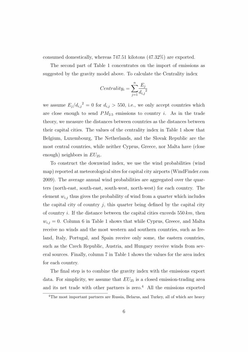
consumed domestically, whereas 747.51 kilotons (47.32%) are exported.
The second part of Table 1 concentrates on the import of emissions as
suggested by the gravity model above. To calculate the Centrality index
Centralityi =n∑
j=1
Ej
di,j2
we assume Ej/di,j2 = 0 for di,j > 550, i.e., we only accept countries which
are close enough to send PM2.5 emissions to country i. As in the trade
theory, we measure the distances between countries as the distances between
their capital cities. The values of the centrality index in Table 1 show that
Belgium, Luxembourg, The Netherlands, and the Slovak Republic are the
most central countries, while neither Cyprus, Greece, nor Malta have (close
enough) neighbors in EU25.
To construct the downwind index, we use the wind probabilities (wind
map) reported at meteorological sites for capital city airports (WindFinder.com
2009). The average annual wind probabilities are aggregated over the quar-
ters (north-east, south-east, south-west, north-west) for each country. The
element wi,j thus gives the probability of wind from a quarter which includes
the capital city of country j, this quarter being defined by the capital city
of country i. If the distance between the capital cities exceeds 550 km, then
wi,j = 0. Column 6 in Table 1 shows that while Cyprus, Greece, and Malta
receive no winds and the most western and southern countries, such as Ire-
land, Italy, Portugal, and Spain receive only some, the eastern countries,
such as the Czech Republic, Austria, and Hungary receive winds from sev-
eral sources. Finally, column 7 in Table 1 shows the values for the area index
for each country.
The final step is to combine the gravity index with the emissions export
data. For simplicity, we assume that EU25 is a closed emission-trading area
and its net trade with other partners is zero.4 All the emissions exported
4The most important partners are Russia, Belarus, and Turkey, all of which are heavy
6
1 2 3 4 5 6 7 8 9
EU25 Emission Radius Domest. Export Centrality Downwind Area Import Total
ktn km ktn ktn index index index ktn ktn
Austria 28.18 163.39 9.13 19.05 1.02 1.45 0.021 49.87 59.00
Belgium 32.86 98.58 9.24 23.62 1.77 1.00 0.007 21.63 30.87
Cyprus 2.18 54.26 0.58 1.60 0.00 0.00 0.002 0.00 0.58
Czech Rep. 42.69 158.44 13.66 29.03 1.22 1.35 0.019 52.10 65.75
Denmark 25.97 117.12 7.56 18.41 0.50 0.42 0.011 3.59 11.15
Estonia 21.69 119.98 6.35 15.34 0.47 1.00 0.011 8.54 14.89
Finland 28.26 328.08 14.90 13.36 0.36 0.86 0.083 41.61 56.51
France 328.23 453.26 253.76 74.47 0.52 0.99 0.159 132.35 386.11
Germany 159.86 337.11 86.71 73.15 0.67 0.94 0.088 90.53 177.24
Greece 47.32 204.93 17.15 30.17 0.00 0.00 0.032 0.00 17.15
Hungary 52.38 172.08 17.35 35.03 0.72 1.49 0.023 39.99 57.34
Ireland 14.16 149.57 4.43 9.73 0.24 0.23 0.017 1.52 5.95
Italy 150.27 309.65 74.80 75.47 0.02 0.26 0.074 0.77 75.57
Latvia 10.93 143.39 3.37 7.56 0.26 0.85 0.016 5.75 9.12
Lithuania 12.5 141.05 3.83 8.67 0.60 0.94 0.015 14.06 17.90
Luxemb. 2.73 0.91 0.70 2.03 1.63 0.96 0.000 0.00 0.70
Malta 0.59 10.03 0.15 0.44 0.00 0.00 0.000 0.00 0.15
Netherl. 26.78 114.97 7.77 19.01 1.27 1.24 0.010 26.26 34.02
Poland 202.7 315.48 102.76 99.94 0.55 1.18 0.077 80.72 183.48
Portugal 76.99 171.49 25.46 51.53 0.30 0.31 0.023 3.48 28.94
Slovak Rep. 14.5 124.69 4.29 10.21 1.25 0.64 0.012 15.72 20.01
Slovenia 12.08 80.33 3.30 8.78 0.69 1.09 0.005 6.09 9.39
Spain 151.14 400.85 99.85 51.29 0.15 0.39 0.124 12.17 112.01
Sweden 25.4 378.45 15.67 9.73 0.20 1.03 0.111 37.77 53.44
United Kgd. 109.4 279.16 49.52 59.88 1.17 0.90 0.060 102.99 152.51
Sum 1579.79 832.28 747.51 747.51 1579.79
Table 1: Emissions, exports, imports, and total deposits in 2000.
7

from EU25 are25∑
j=1
EXj (747.51 kilotons, Table 1). The crucial simplifying
trick is that since the gravity index takes care of the imports of individual
countries, we can simply distribute the total bulk of exports to countries
according to this index to get
IMi =25∑
j=1
EXj ×Gravityi, (6)
where IMi is the import of emissions in country i.
Column 8 in Table 1 reports emission imports, and the last column adds
imports and domestic consumption to total deposits. To take an example,
note that out of its emissions of 28.18 kilotons, Austria consumes 9.13 kilotons
domestically and exports 19.05 kilotons. Given that its imports are 49.87
kilotons, its total deposit ends up as 59.00 kilotons, so that Austria, as a
relatively central and large downwind country, is a heavy net importer of
emissions.
0
50
100
150
200
250
Deposits / Emissions (%)
Austr
ia
Belg
ium
Cypru
s
Czech
Denm
ark
Esto
nia
Fin
land
Fra
nce
Germ
any
Gre
ece
Hungary
Irela
nd
Italy
Latv
ia
Lithuania
Luxe
mb.
Malta
Neth
erl
.
Pola
nd
Port
ugal
Slo
vak
Slo
venia
Spain
Sw
eden
United K
.
Figure 1: Deposits/Emissions (%).
polluters, but located downwind from EU25. Some pollutants may also arrive in EU25
overseas from North America and Africa. Since the data is taken from the CAFE project ofthe European Union, they are only available to EU25-countries, also leaving some Europeancountries out of this analysis.
8

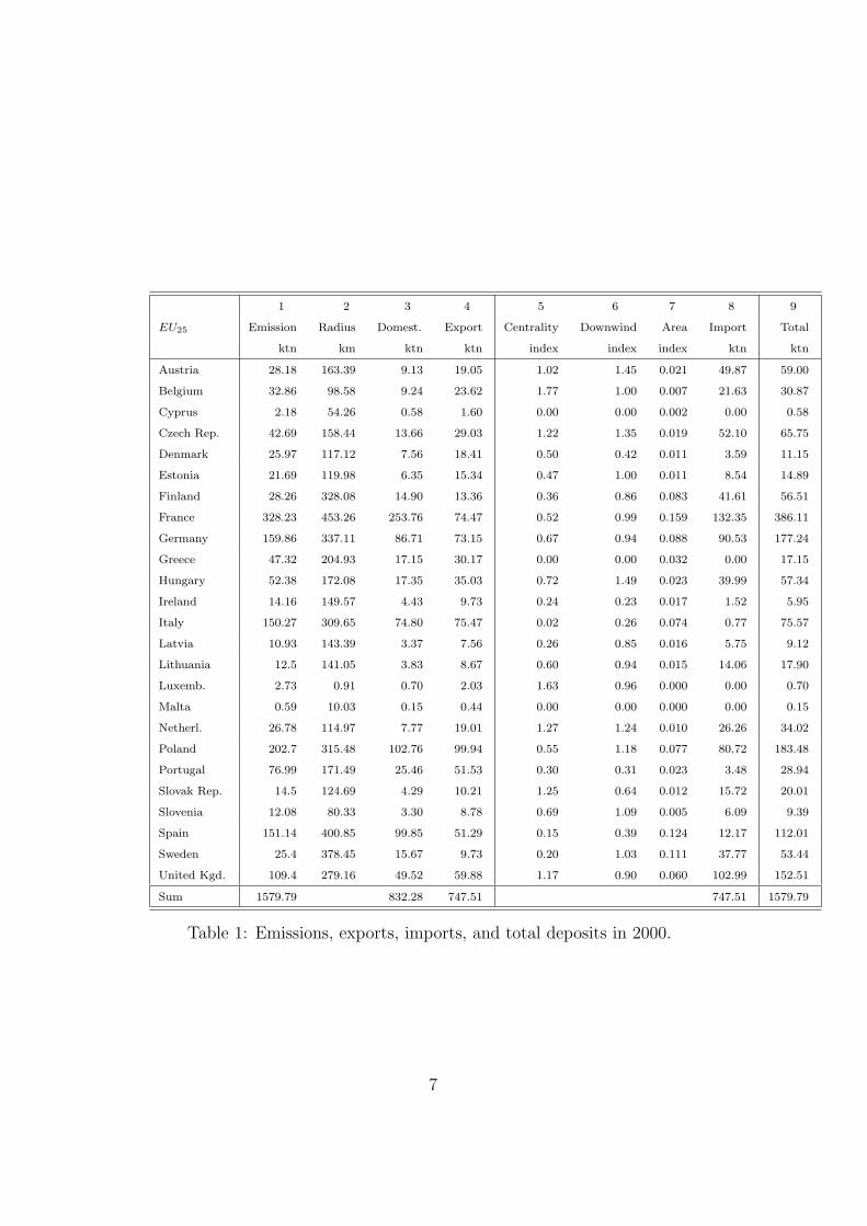
Figure 1 illustrates the results from Table 1 by scaling down the emis-
sions to 100 for each country. Thus the number for Austria is derived from
(59.00/28.18) ∗ 100 = 209.36 (columns 9 and 1). Figure 1 shows that the
countries in EU25 seem to constitute four categories. The first category is the
smallest countries (Cyprus, Luxemburg, Malta) with a low deposit/emission
ratio (< 30%), then comes a group net exporters with deposit/emission ra-
tio of 30 − 80% (Greece, Portugal, Ireland, Denmark, Italy, Estonia, Spain,
Slovenia), and the third group has a deposit/emission ratio of 80 − 120%
(Latvia, Poland, Belgium, Hungary, Germany, France). Finally, there is a
group of heavy net importers, (Netherlands, the Slovak Republic, the United
Kingdom, Lithuania, the Czech Republic, Finland, Austria, and Sweden)
with a deposit/emission ratio of > 120%. The three heaviest net importers,
Finland, Austria, and Sweden, are large countries in the eastern or north-
ern part of Europe, i.e., receiving permanent winds from other countries in
EU25, and not even their distant location can spare them from the emissions
of their neighbors. These heaviest net importers receive so much that their
total deposits are twice their own emissions.
The results of the current paper can be compared to those derived by
alternative methods. Niemi et al. (2009), by using several methodologies,
such as air quality monitoring, backward air mass trajectories, and chemical
analysis of particle samples, found that 50−75% of the PM2.5 mass in urban
areas in Finland originates from long-range transportation. Karppinen et al.
(2004) construct and test a linear regression model and found that the long-
range transportation contributes to 64− 76% of the PM2.5 concentration in
the urban air in Helsinki (Finland). These results are in line with the estimate
of 73.63% derived in this paper. An interesting comparison is that with
Tainio et al. (2009) who have derived results for Europe by using the intake
fraction approach. For EU25, the correlation between the total deposits from
Tainio et al. (2009) and from this paper is as high as 84.83%. However, our
estimates are smaller in western countries, Portugal, Italy, and Greece, for
9

example, but larger in eastern countries, such as Lithuania, Slovenia, Sweden,
Austria, Finland, and Estonia, implying that our estimates may suffer from
a somewhat excessive emphasis on wind. Another possibility is that the
wind direction, taken from WindFinder.com (2009) and indicating the low-
atmospheric situation alone, should be replaced by winds at higher altitudes,
probably with larger relevance to pollution transfers but, unfortunately, such
a wind map is not available to the authors yet.
4 Emissions and economic growth
In this section, we evaluate the future emissions. Since the PM2.5 emis-
sions are mainly generated from economic activities, such as production,
consumption, and transportation, as summarized in the gross national prod-
uct (GDP), in projecting emissions, the association between incomes and
emissions needs to be estimated. Unfortunately, data on PM2.5 is available
only for a single year (2000), making country-specific time series analysis
impossible. Therefore, we turn to the alternative approach and estimate the
emission-income association from a cross-section of countries. Given that the
GDPs of the EU25 members are of different magnitudes, we first integrate
the data by utilizing the EKC decomposition.
4.1 The EKC decomposition
The Environmental Kuznets Curve (EKC ) claims that the impact of eco-
nomic growth (i.e., the increase in the per capita GDP) on pollution is
dictated by two effects. On the one hand, the adoption and implemen-
tation of cleaner production techniques and the shift to services tends to
decrease the emission intensity of the GDP, but the increase in per capita
GDP tends to work in the opposite direction because of higher consump-
tion (Arrow et al. 1995, Grossman and Krueger 1995). These effects are
known as technology-composition and scale effects respectively. Since emis-
10

sion intensities can be directly compared between countries, we estimate the
technology-composition effect from a cross-section of countries and derive the
full expression for country-specific emissions mathematically.5
Consider the emission intensity of GDP, defined by φ = E/GDP with E
referring to PM2.5 emissions as before.6 Figure 2 illustrates the values of φ as
a function of the real GDP per capita (GDPpc) in 2000 for EU25, showing
that richer countries use cleaner production techniques than poorer coun-
tries. Several formulas (hyperbolic, exponential, logarithmic) can capture
the association between incomes and emissions, but the highest explanatory
power is provided by φ = α ·GDPpcβ. Hence, by taking logs, we fit
ln φi,2000 = ln α + β · ln GDPpci,2000 + εi,2000 (7)
by OLS. The derived estimates are α = 56298.77 and β = −1.27. Formula
(7) explains 55% of the cross-sectional variation in φ.
0 50000
GDP per capita
0
0.5
1
1.5Emission intensity φ
0 10000 20000 30000 400000
0.5
1
1.5
Figure 2: Emission intensity of output φ as a function of real GDP per capita(GDPpc) in 2000, EU25.
The definition φ = E/GDP implies E = φ ·GDP = φ ·GDPpc ·L, where
L is population. Applying this to GDPpc and population L in country i at
5Testing the Environmental Kuznets Curve hypothesis which claims that pollution firstincreases but then decreases along with economic growth is beyond the scope of the currentpaper.
6The data for GDPpc comes from Heston et al. (2006).
11

time t, one can derive the country-specific emission functions
Ei,t = li · 56298.77 ·GDPpc−0.27i,t · Li,t, (8)
where the multiplicative fixed factor li is the residual from (7) divided by
φi,2000. Equation (8) shows that the elasticity of emissions with respect to
the GDPpc (L) is a negative (positive) constant. Thus, in spite of decreasing
emission intensities, the emissions themselves may increase or decrease over
time, depending upon the growth rates of GDPpc and L.7
4.2 Income, population, and emissions
To provide country-specific projections for emissions in 2020 from (8) we
estimate the values for GDPpci,2020 from the time series of GDPpci,1950−2003
by applying linear trends, with country-specific breaks being allowed for the
1973-1982 and 1990-1992 periods. The former break counts the oil crises and
the latter the collapse of the Soviet Union. Column 1 in Table 2 shows the
projected values for GDPpc, column 2 reports R2 and column 3 provides
the implied growth rate of GDPpc, which is 2.55% on average for EU25.
For Li,2020 we utilize the medium variant projection from the United Nations
(2007) (column 4), and the implied population growth rates are shown in
column 5. Column 6 shows the emissions in 2020 calculated from equation
(8).
Repeating the procedure in Section 3, one can now calculate the exported
and imported emissions in 2020. Note that the centrality index needs to be
updated for emissions in 2020, but the downwind and area indices remain
constant. Ultimately, one can calculate the total deposits in 2020 shown in
column 7 of Table 2 and indicating that total emissions in EU25 will decrease
from 1579.79 to 1468.22 kilotons.
7Note that (7) (and (8) as derived from (7)) pays no attention to new abatement policiesor to innovations in decreasing emissions. In this sense, it can be thought of as a minimumvariant for emission decreases in the future.
12

1 2 3 4 5 6 7
EU25 GDPpc R2 Growth POP POP Emissions Deposits
$ % thousand growth % ktn ktn
Austria 40220.3 1 1.99 8575.29 0.29 26.77 52.90
Belgium 35445.46 1 1.81 10684.12 0.18 30.86 30.37
Cyprus 56140.91 0.99 5.05 975.21 1.26 2.13 0.56
Czech Re. 18304.08 0.7 1.48 10042.94 -0.11 38.51 57.93
Denmark 37449.54 0.99 1.48 5543.82 0.19 24.86 10.62
Estonia 19721.31 0.53 2.88 1277.64 -0.57 16.54 12.90
Finland 30990.49 0.99 1.55 5433.57 0.24 27.26 48.06
France 35026.15 1 1.68 64824.74 0.45 327.49 382.87
Germany 31851.92 1 1.2 81160.69 -0.07 147.57 156.84
Greece 17441.96 0.99 1.11 11274.29 0.13 45.76 16.58
Hungary 19983.82 0.98 2.81 9620.66 -0.3 42.25 48.02
Ireland 47288.03 0.99 3.2 5055.46 1.43 15.81 6.45
Italy 33390.83 1 1.98 58600.98 0.08 136.95 68.84
Latvia 23234.71 0.96 4.74 2133.68 -0.6 7.48 7.32
Lithuania 23409 0.93 4.69 3187.83 -0.64 8.52 13.56
Luxemb. 93296.29 1 3.3 538.28 1.06 2.82 0.73
Malta 47439.06 1 4.61 426.48 0.43 0.5 0.13
Netherl. 34939.45 0.99 1.42 16760.03 0.26 26.12 33.70
Poland 18524.68 0.96 3.83 37079.18 -0.21 157.72 151.99
Portugal 28380.16 0.99 2.47 10790.29 0.27 70.99 27.09
Slovak Re. 15382.81 0.94 2.31 5365.85 -0.03 12.7 17.40
Slovenia 33080.58 0.88 2.99 1972.28 0.11 10.5 8.36
Spain 28642.61 1 1.91 46445.21 0.66 155.28 113.92
Sweden 32562.58 1 1.28 9652.45 0.42 25.76 49.16
United Kgd 36745.56 1 1.99 64033.23 0.44 107.08 151.95
Sum/Aver. 33555.69 0.95 2.55 471454.19 0.21 1468.22 1468.22
Table 2: Income, population, emissions, and total deposition in 2020.
13

Figure 3 illustrates the results of Table 2 by scaling the numbers for 2000
down to 100, which shows that considerable differences between countries
will arise both in terms of economic and population growth. In Cyprus, for
example, the average economic growth from 2003 to 2020 (panel a) will be
5.05%, causing a considerable tendency to a decrease in emissions. On the
other hand, Cyprus will also face the highest population growth, which annuls
the decrease in emissions (panels b and c). The same type of development is
foreseen in Ireland. In contrast, high economic growth in Hungary, Latvia,
Lithuania, and Poland is supported by low population growth, leading to a
greater than average decrease in emissions. Panel d shows, however, that the
change in deposits is much more evenly distributed than that in emissions,
as the situation of neighboring countries also contributes to it.
0
50
100
150
GDP per capita 2020 Population 2020
Emissions 2020 Deposits 2020
a) b)
c) d)
Austr
ia
Belg
ium
Cypru
s
Czech
Denm
ark
Esto
nia
Fin
land
Fra
nce
Germ
any
Gre
ece
Hungary
Irela
nd
Italy
Latv
ia
Lithuania
Luxe
mb.
Malta
Neth
erl
.
Pola
nd
Port
ugal
Slo
vak
Slo
venia
Spain
Sw
eden
United K
.
Austr
ia
Belg
ium
Cypru
s
Czech
Denm
ark
Esto
nia
Fin
land
Fra
nce
Germ
any
Gre
ece
Hungary
Irela
nd
Italy
Latv
ia
Lithuania
Luxe
mb.
Malta
Neth
erl
.
Pola
nd
Port
ugal
Slo
vak
Slo
venia
Spain
Sw
eden
United K
.
Austr
ia
Belg
ium
Cypru
s
Czech
Denm
ark
Esto
nia
Fin
land
Fra
nce
Germ
any
Gre
ece
Hungary
Irela
nd
Italy
Latv
ia
Lithuania
Luxe
mb.
Malta
Neth
erl
.
Pola
nd
Port
ugal
Slo
vak
Slo
venia
Spain
Sw
eden
United K
.
Austr
ia
Belg
ium
Cypru
s
Czech
Denm
ark
Esto
nia
Fin
land
Fra
nce
Germ
any
Gre
ece
Hungary
Irela
nd
Italy
Latv
ia
Lithuania
Luxe
mb.
Malta
Neth
erl
.
Pola
nd
Port
ugal
Slo
vak
Slo
venia
Spain
Sw
eden
United K
.
020406080
100120140160180200220240260280300
0
20
40
60
80
100
120
0
20
40
60
80
100
120
Figure 3: A comparison between the years 2000 and 2020. The values for2000 = 100.
14

5 Sensitivity analysis of emissions
According to (8), the main determinants of emissions are income and popu-
lation, the projections of which are provided in Table 2. This Section aims to
quantify the uncertainty in these projections by providing alternative num-
bers. Since total deposits depend on emissions in neighboring countries, they
are rather complicated to interpret. The sensitivity results are thus reported
here only in terms of emissions.
The estimates of the income trends provide standard 95% confidence lim-
its, showing that the implied average economic growth from 2003 to 2020,
which in the basic case was 2.55%, becomes 1.31% in the case of the lower
confidence limit and 3.79% in the higher. Given the negative elasticity of
emissions in terms of incomes [Cf. (8)], one expects to see lower emissions
for the higher confidence limit of GDPpc and vice versa.
0
20
40
60
80
100
120
140
%
Au
str
ia
Be
lgiu
m
Cyp
rus
Cze
ch
De
nm
ark
Esto
nia
Fin
lan
d
Fra
nce
Ge
rma
ny
Gre
ece
Hu
ng
ary
Ire
lan
d
Ita
ly
La
tvia
Lith
ua
nia
Lu
xem
b.
Ma
lta
Ne
the
rl.
Po
lan
d
Po
rtu
ga
l
Slo
vak
Slo
ven
ia
Sp
ain
Sw
ed
en
Un
ite
d K
. 0
20
40
60
80
100
120
%
Au
str
ia
Be
lgiu
m
Cyp
rus
Cze
ch
De
nm
ark
Esto
nia
Fin
lan
d
Fra
nce
Ge
rma
ny
Gre
ece
Hu
ng
ary
Ire
lan
d
Ita
ly
La
tvia
Lith
ua
nia
Lu
xem
b.
Ma
lta
Ne
the
rl.
Po
lan
d
Po
rtu
ga
l
Slo
vak
Slo
ven
ia
Sp
ain
Sw
ed
en
Un
ite
d K
.
GDP per capita Population
a b
Figure 4: The confidence interval of emissions for GDPpc and population in2020.
Figure 4a shows that this is indeed the case. Normalizing the emissions
in 2000 to 100, the higher confidence limit for income (grey bar) shows the
emission that will be below it (94.99 on the average), whereas the lower
confidence limit (grey + black bar) shows emissions above it (104.65, on
average). The black bar shows the confidence interval, which in most cases
15

is narrow, the smallest values being seen in the old EU members, such as
Belgium, France, and Austria. New members, such as the Slovak Republic,
Hungary, and Estonia exhibit largest confidence intervals, but this difference
is mostly due to shorter GDPpc series from these countries. In contrast,
relatively large confidence intervals in Finland, Ireland, and Luxembourg,
indicate a genuine variation in their growth histories since data from these
countries is in time series as long as from other older members.
0
20
40
60
80
100
120
140
%
Austr
ia
Belg
ium
Cypru
s
Czech
Denm
ark
Esto
nia
Fin
land
Fra
nce
Germ
any
Gre
ece
Hungary
Irela
nd
Italy
Latv
ia
Lithuania
Luxe
mb.
Malta
Neth
erl
.
Pola
nd
Port
ugal
Slo
vak
Slo
venia
Spain
Sw
eden
United K
.
Figure 5: The worst-worst versus best-best confidence interval of emissions2020.
The population projections in Table 2 come from The United Nations
(2007), and are available in three variants, low, medium, and high. These
variants mainly differ in terms of fertility behavior, but other factors, such
as immigration, are also considered. The numbers in Table 2 refer to the
medium variant, so that we can recalculate the emissions in 2020 for low
and high variants. The medium variant projection for 2020 for the total
population in EU25 is 471, 454 thousand people, whereas the low and high
variant projections are 454, 661 and 488, 074 correspondingly, the difference
between the latter two being 7.34%. The emission calculations, which are
performed under the assumption that GDPpc proceeds as rapidly as in the
benchmark projection in spite of higher population growth, show that this
difference is almost directly transformed into a difference in emissions, which
for the low and high variants is 1415.34 and 1520.52 with a difference of
7.43%, respectively, i.e., the demographic uncertainty generates almost as
16
high uncertainty in emissions as the economic growth. Nevertheless, this
risk is much more evenly distributed among countries [Figure 4b].
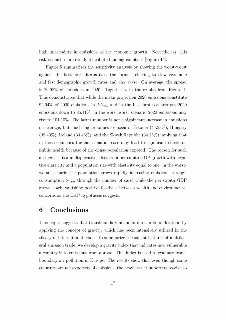
Figure 5 summarizes the sensitivity analysis by showing the worst-worst
against the best-best alternatives, the former referring to slow economic
and fast demographic growth rates and vice versa. On average, the spread
is 20.98% of emissions in 2020. Together with the results from Figure 4.
This demonstrates that while the mean projection 2020 emissions constitute
92.94% of 2000 emissions in EU25, and in the best-best scenario get 2020
emissions down to 85.41%, in the worst-worst scenario 2020 emissions may
rise to 101.10%. The latter number is not a significant increase in emissions
on average, but much higher values are seen in Estonia (44.33%), Hungary
(39.40%), Ireland (34.46%), and the Slovak Republic (34.26%) implying that
in these countries the emissions increase may lead to significant effects on
public health because of the dense population exposed. The reason for such
an increase is a multiplicative effect from per capita GDP growth with nega-
tive elasticity and a population size with elasticity equal to one: in the worst-
worst scenario the population grows rapidly increasing emissions through
consumption (e.g., through the number of cars) while the per capita GDP
grows slowly vanishing positive feedback between wealth and environmental
concerns as the EKC hypothesis suggests.
6 Conclusions
This paper suggests that transboundary air pollution can be understood by
applying the concept of gravity, which has been intensively utilized in the
theory of international trade. To summarize the salient features of multilat-
eral emission trade, we develop a gravity index that indicates how vulnerable
a country is to emissions from abroad. This index is used to evaluate trans-
boundary air pollution in Europe. The results show that even though some
countries are net exporters of emissions, the heaviest net importers receive so
17

much that their total deposits are up to twice their own emissions, implying
that transboundary air pollution is a serious problem in these countries.
Since air pollution is mainly generated from economic activities such as
production, consumption, and transportation, summarized in the gross na-
tional product, we estimate the association between the GDP and emissions
by utilizing the EKC decomposition. It turns out that richer countries use
cleaner production techniques making the elasticity of emissions in terms of
income negative. However, because the elasticity of emissions in terms of
population is positive, emissions may increase or decrease over time, depend-
ing upon the economic and demographic growth rates.
We thus provide country-specific estimates the values for per capita in-
comes and population in 2020 and calculate emissions and total deposits in
2020, indicating that total emissions in EU25 will decrease from 1579.79 to
1468.22 kilotons. Given that considerable differences between countries will
arise both in terms of economic and population growth, the decrease in emis-
sions varies to a great extent. The decrease in deposits, however, is much
more evenly distributed because emissions trading exposes even the emission
decreasing countries to emissions import from abroad. Therefore, emission
decreases in individual countries will be annulled unless the emission decrease
are concomitant in Europe.
18

References
Amann M, Cofala J, Gzella A, Heyes Ch, Klimont Zb, Schopp W (2007):
Estimating Concentrations of Fine Particulate Matter in Urban Background
Air of European Cities. IIASA Interim Report IR-007-01.
Arrow K, Bolin B, Costanza R, Dasgupta P, Folke K, Holling CS, Jansson
BO, Levin S, Maler KG, Perrings C, Pimentel D (1995): Economic Growth,
Carrying Capacity, and the Environment, Ecological Economics 15, 91–95.
Borge R, Lumbreras J, Vardouakis S, Kassomens P, Rodrıgues E (2007):
Analysis of Long-Range Transport Influences on Urban PM10 using Two-
Stage Atmospheric Trajectory Clusters, Atmospheric Environment 41, 4434–
4450.
Cohen AJ, Anderson RH, Ortro B, Dev Pandey K,Krzyzanowski M, Kunzli
N, Gutschmidt K, Pope III AC, Romieu I, Samet JM, Smith KR (2004):
Mortality Impacts of Urban Air Pollution. In Ezzati M, Lopez AD, Rogers
A, Murray CLJ (eds). Comparative Quantification of Health Risks: Global
and Regional Burden of Disease Attributable to Selected Major Risk Factors.
Geneva, WHO, Vol 2, 1353–1433.
Greco, Susan L, Wilson, Andrew M, Spengler, John D. and Levy, Jonathan
I (2007): Spatial Patterns of Mobile Source Particulate Matter Emission-to
Exposure Relationships across the United States. Atmospheric Environment
41, 1011–1025.
Grossman GM, Krueger AB (1995): Economic Growth and the Environment.
Quarterly Journal of Economics 110, 9353–9377.
Harrigan J (2003): Specialization and the Volume of Trade: Do the Data
obey the Laws In Aldrich WM, Choi EK and Harrigan J (Editors), Handbook
of Internatioal Trade. Blackwell, Chicago (Chapter 21).
Helliwell JF (1997): National Borders, Trade and Migration. NBER working
Paper Series No. 6027.
19

Helliwell JF (1998): How Much do National Borders Matter? The Brookings
Institution, Washington DC.
Heston A, Summers R, and Aten B (2006): Penn World Table Version 6.2,
Center for International Comparison of Production, Income and Prices at
the University of Pennsylvania.
Karppinen A, Harkonen J, Kukkonen J, Aarnio P, Koskentalo T. (2004):
Statistical model for assessing the portion of fine particulate matter trans-
ported regionally and long range to urban air. Scand J Work Environ Health,
Suppl. 2, 47–53.
McCallum J (1995): National Borders Matter. American Economic Review
85(3), 615–623.
Moussiopoulos N, Helmis CG, Folcas HA, Louka P, Assimakopoulos VD,
Naneris C, Sahm P(2004): A Modelling Method for Estimating Transbound-
ary Air Pollution in Southeastern Europe. Environmental Modelling & Soft-
ware 19, 547–558.
Niemi JV, Saarikoski S, Aurela M, Tervahattu H, Hillamo R, Westphal DL,
Aarnio P, Koskentalo T, Makkonen U, Vehkamaki H, Kulmala M (2009):
Long-Range Transport Episodes of Fine Particles in Southern Finland During
1999-2007. Atmospheric Environment 43, 1255–1264.
Nigge, K-M (2001): Generic Spatial Classes for Human Health Impacts, Part
I: Methodology. International Journal of Life Cycle Assessment 6, 257–264.
Scheringer (2009): Long-Range Transport of Organic Chemicals in the En-
vironment. Environmental Toxicology and Chemistry 28(4), 677–690.
Tainio, M., Sofiev, M., Hujo, M., Tuomisto, J., Loh, M., Jantunen, M., Karp-
pinen, A., Knagas, L., Karvosenoja, N., Kupiainen, K., Porvari, P., Kukko-
nen., J. (2009): Evaluation of the European Intake Fractions for European
and Finnish Anthropogenetic Primary Fine Particulate Matter Emissions.
Atmospheric Environment 43, 3052–3059.
20

WindFinder.com e.K. (2009): Historical Wind Statistics. Online data.
United Nations (2007). World Population Prospects. The 2006 revision.
New York.
21