Embed Size (px)
Citation preview
December 2011 National Collaborating Centre for Environmental Health
Air Quality Assessment Tools:
A Guide for Public Health Practitioners
Prabjit Barn, Peter Jackson, Natalie Suzuki, Tom Kosatsky, Derek Jennejohn, Sarah Henderson, Warren McCormick, Gail Millar, Earle Plain, Karla Poplawski, Eleanor Setton
Summary
• Several tools exist to assess local air quality, including the impact of specific sources, emissions, and meteorological conditions.
• Information generated from the use of air quality assessment tools can inform decisions on permitting of emissions, industrial siting, and land use; all can impact local air quality, which in turn can influence air pollution related health effects of a population.
• The five tools discussed in this guide (highlighted with case examples) address different components of air quality:
o Emissions inventories are databases of air pollution sources and their emissions, which allow for the monitoring of pollution releases to the air; emissions inventories can feed into other tools, such as dispersion models.
o Dispersion modeling uses data on emissions, meteorology, and topography to provide estimates of ambient pollutant concentrations at specific receptor sites.
o Source apportionment helps to identify important sources in an area by using information on ambient pollutant levels.
o Mobile monitoring, in contrast to traditional fixed site monitoring, allows for a better understanding of pollutant concentrations and their sources, both temporally and, very importantly, spatially; Data collected by mobile monitoring projects can feed into models, such as land-use regression.
o Land use regression uses a combination of local information to provide the best estimates of ambient pollution in a specific area.
• Health impact assessment is an example of direct application of information generated by air quality assessment tools, to understand the air quality related health impacts of a population.
Introduction
Air quality impacts both the environment and health. Air quality management aims to limit negative impacts through a variety of activities, including legislation, policies, and plans to manage emissions and monitor ambient air quality. Air quality assessments inform air quality management activities by providing an understanding of how pollutant sources, emission characteristics, topography, and meteorological conditions contribute to local air quality. Specific
December 2011 National Collaborating Centre for Environmental Health 2
air quality assessment tools can help answer a variety of questions which are integral to air quality management activities, including:
• How can frequently poor air quality be improved? • Which source(s) or source sectors contribute to poor air quality? • How can air quality impacts be minimized? • Which regions are most affected? • Should existing sources be targeted for emissions reductions? • What location, for new sources, could minimize air quality impacts? • Will emissions from a proposed new source result in a substantial degradation in air
quality?
Although air quality assessment tools are valuable when informing decisions that impact local air quality, their use may be overlooked by public health practitioners. The information conveyed by these tools is often highly technical and typically accessible only to trained air quality management personnel. As a result, useful information may not be available to support decisions on emissions permitting, industrial siting, and land use, as well as the development of public health messages. The objective of this guide is to increase the understanding and accessibility of these tools to better support public health responses and policy decisions on local air quality. The specific assessment tools discussed in this guide are: (1) emissions inventories, (2) dispersion modelling, (3) source apportionment, (4) mobile monitoring, and (5) land use regression. Health Impact Assessment is discussed as a direct application of information provided by air quality assessment tools.
A brief overview of key sources and pollutants in British Columbia (BC) and their health impacts is provided to give context to the tools. A description of the BC air quality monitoring network, current practices in BC, regarding land use, emissions permitting, and health messaging, follows. The remainder of the guide provides a description of each tool, as well as advantages and limitations of their use. Finally, local examples are provided for each tool, to highlight their use in air quality management in the province.
Key Pollutants and Sources
Pollutants
Air pollutants are gases or particles in the atmosphere which have been linked to harmful human health or environmental effects. Pollutants can be categorized according to their formation (primary or secondary), their sources, and their chemical composition and characteristics.
Pollutants can be primary or secondary. Primary pollutants are released directly into the atmosphere while secondary pollutants are formed through reactions between pollutants already present in the atmosphere, also known as precursors. Fine particulate matter (particles smaller than 2.5 µm in aerodynamic diameter) is an example of both a primary and secondary pollutant. These particles can be formed directly through combustion processes, including activities involving wood burning or vehicle engines, and can also be formed through reactions between pollutants, such as nitrogen oxides (NOx), volatile organic compounds (VOCs), and sulfur oxides (SOx). Ground level ozone is a secondary pollutant that is formed through reactions between NOx and VOCs in the presence of sunlight.
Environment Canada classifies major pollutants into four main groups; 1) criteria air contaminants, 2) persistent organic pollutants, 3) heavy metals, and 4) Toxics.1 Criteria air
December 2011 National Collaborating Centre for Environmental Health 3
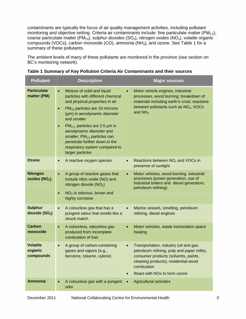
contaminants are typically the focus of air quality management activities, including pollutant monitoring and objective setting. Criteria air contaminants include: fine particulate matter (PM2.5), coarse particulate matter (PM10), sulphur dioxides (SOx), nitrogen oxides (NOx), volatile organic compounds (VOCs), carbon monoxide (CO), ammonia (NH3), and ozone. See Table 1 for a summary of these pollutants.
The ambient levels of many of these pollutants are monitored in the province (see section on BC’s monitoring network).
Table 1 Summary of Key Pollution Criteria Air Contaminants and their sources
Pollutant Description Major sources
Particulate matter (PM)
• Mixture of solid and liquid particles with different chemical and physical properties in air
• PM10 particles are 10 microns (µm) in aerodynamic diameter and smaller
• PM2.5 particles are 2.5 µm in aerodynamic diameter and smaller; PM2.5 particles can penetrate further down in the respiratory system compared to larger particles
• Motor vehicle engines, industrial processes, wood burning; breakdown of materials including earth’s crust; reactions between pollutants such as NOx, VOCs and NH3
Ozone • A reactive oxygen species • Reactions between NOx and VOCs in presence of sunlight
Nitrogen oxides (NOx)
• A group of reactive gases that include nitric oxide (NO) and nitrogen dioxide (NO2)
• NO2 is odorous, brown and highly corrosive
• Motor vehicles, wood burning, industrial processes (power generation, use of industrial boilers and diesel generators, petroleum refining)
Sulphur dioxide (SO2)
• A colourless gas that has a pungent odour that smells like a struck match.
• Marine vessels, smelting, petroleum refining, diesel engines
Carbon monoxide
• A colourless, odourless gas produced from incomplete combustion of fuel.
• Motor vehicles, waste incineration space heating
Volatile organic compounds
• A group of carbon-containing gases and vapors (e.g., benzene, toluene, xylene)
• Transportation, industry (oil and gas, petroleum refining, pulp and paper mills), consumer products (solvents, paints, cleaning products), residential wood combustion
• React with NOx to form ozone
Ammonia • A colourless gas with a pungent odor
• Agricultural activities
December 2011 National Collaborating Centre for Environmental Health 4
Sources
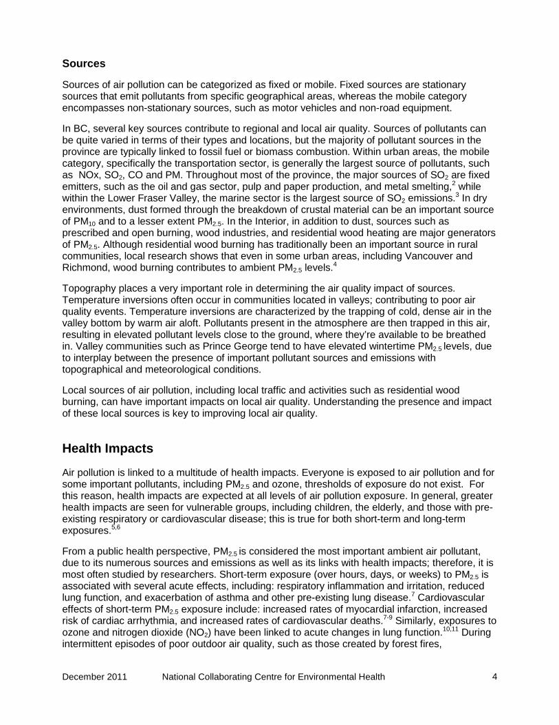
Sources of air pollution can be categorized as fixed or mobile. Fixed sources are stationary sources that emit pollutants from specific geographical areas, whereas the mobile category encompasses non-stationary sources, such as motor vehicles and non-road equipment.
In BC, several key sources contribute to regional and local air quality. Sources of pollutants can be quite varied in terms of their types and locations, but the majority of pollutant sources in the province are typically linked to fossil fuel or biomass combustion. Within urban areas, the mobile category, specifically the transportation sector, is generally the largest source of pollutants, such as NOx, SO2, CO and PM. Throughout most of the province, the major sources of SO2 are fixed emitters, such as the oil and gas sector, pulp and paper production, and metal smelting,2 while within the Lower Fraser Valley, the marine sector is the largest source of SO2 emissions.3 In dry environments, dust formed through the breakdown of crustal material can be an important source of PM10 and to a lesser extent PM2.5. In the Interior, in addition to dust, sources such as prescribed and open burning, wood industries, and residential wood heating are major generators of PM2.5. Although residential wood burning has traditionally been an important source in rural communities, local research shows that even in some urban areas, including Vancouver and Richmond, wood burning contributes to ambient PM2.5 levels.4
Topography places a very important role in determining the air quality impact of sources. Temperature inversions often occur in communities located in valleys; contributing to poor air quality events. Temperature inversions are characterized by the trapping of cold, dense air in the valley bottom by warm air aloft. Pollutants present in the atmosphere are then trapped in this air, resulting in elevated pollutant levels close to the ground, where they’re available to be breathed in. Valley communities such as Prince George tend to have elevated wintertime PM2.5 levels, due to interplay between the presence of important pollutant sources and emissions with topographical and meteorological conditions.
Local sources of air pollution, including local traffic and activities such as residential wood burning, can have important impacts on local air quality. Understanding the presence and impact of these local sources is key to improving local air quality.
Health Impacts
Air pollution is linked to a multitude of health impacts. Everyone is exposed to air pollution and for some important pollutants, including PM2.5 and ozone, thresholds of exposure do not exist. For this reason, health impacts are expected at all levels of air pollution exposure. In general, greater health impacts are seen for vulnerable groups, including children, the elderly, and those with pre-existing respiratory or cardiovascular disease; this is true for both short-term and long-term exposures.5,6
From a public health perspective, PM2.5 is considered the most important ambient air pollutant, due to its numerous sources and emissions as well as its links with health impacts; therefore, it is most often studied by researchers. Short-term exposure (over hours, days, or weeks) to PM2.5 is associated with several acute effects, including: respiratory inflammation and irritation, reduced lung function, and exacerbation of asthma and other pre-existing lung disease.7 Cardiovascular effects of short-term PM2.5 exposure include: increased rates of myocardial infarction, increased risk of cardiac arrhythmia, and increased rates of cardiovascular deaths.7-9 Similarly, exposures to ozone and nitrogen dioxide (NO2) have been linked to acute changes in lung function.10,11 During intermittent episodes of poor outdoor air quality, such as those created by forest fires,
December 2011 National Collaborating Centre for Environmental Health 5
researchers find that more people visit doctors’ offices and hospital emergency rooms for respiratory-related effects such as asthma, chronic obstructive pulmonary disease (COPD), and upper respiratory infections.12,13
Long-term exposures to air pollution are also linked to important health impacts; these include increased mortality related to respiratory and cardiovascular disease, increased incidence of asthma, and accelerated development of atherosclerosis.5,7,9 Research, both nationally and internationally have found similar associations between PM exposure and increased mortality.
Research shows that aside from regional impacts, specific sources have an important local impact on air pollution and health. Localized sources, such as traffic and wood smoke have been implicated as sources of pollution hot spots and important contributors to community level health impacts. Exposures to most air pollutants follow a gradient; those living closer to hot spots experience higher exposures compared to those living further away. For example, research indicates that living close to roads may be an independent risk factor for the onset of childhood asthma and may increase the risk of cardiovascular mortality.7 Research conducted within the province confirms the important role that local air pollution plays in contributing to air pollution-related health impacts. Much valuable evidence comes from the BC-Washington State Border Air Quality Study (BAQS), which investigated the air quality-related health impacts of the Georgia Basin-Puget Sound airshed. Researchers found associations between local traffic-related air pollution, including PM2.5 and NO2, and health effects including increased risk of premature births and low birth weight, bronchiolitis, and increased incidence of asthma, among residents living close to traffic sources.14 Research also shows that both proximity of residences to roadways and traffic intensity are linked with adverse respiratory health effects, particularly in children.14,15 Clearly, exposure to air pollution negatively impacts the health of a population. Addressing ways in which to improve local air quality can have important health gains.
Air Quality Management in BC
Air quality management aims to protect air quality through several practices and activities, including: development of legislation and policies to manage emissions; monitoring of ambient air quality; development of provincial air quality objectives; regulation and authorization of pollutant discharges to the environment, including emissions to air as well as the development of regional air shed management plans (in combination with regional authorities). Traditionally, management practices have largely focused on controlling emissions through improved technology and fuel quality, as well as regulation and monitoring of discharges to the air, in order to address specific pollutants and their sources. More recently, land use planning and its impacts on air pollution exposures have begun to be considered as an air quality management tool. This section provides an overview of the provincial monitoring network and briefly discusses the regulatory frameworks of two specific air quality management practices used to address air pollution; permitting of emissions and land use planning.
The Provincial Monitoring Network
The provincial monitoring network provides information on ambient levels of pollution throughout BC. It consists of approximately 150 fixed-site monitoring stations that monitor a combination of
December 2011 National Collaborating Centre for Environmental Health 6
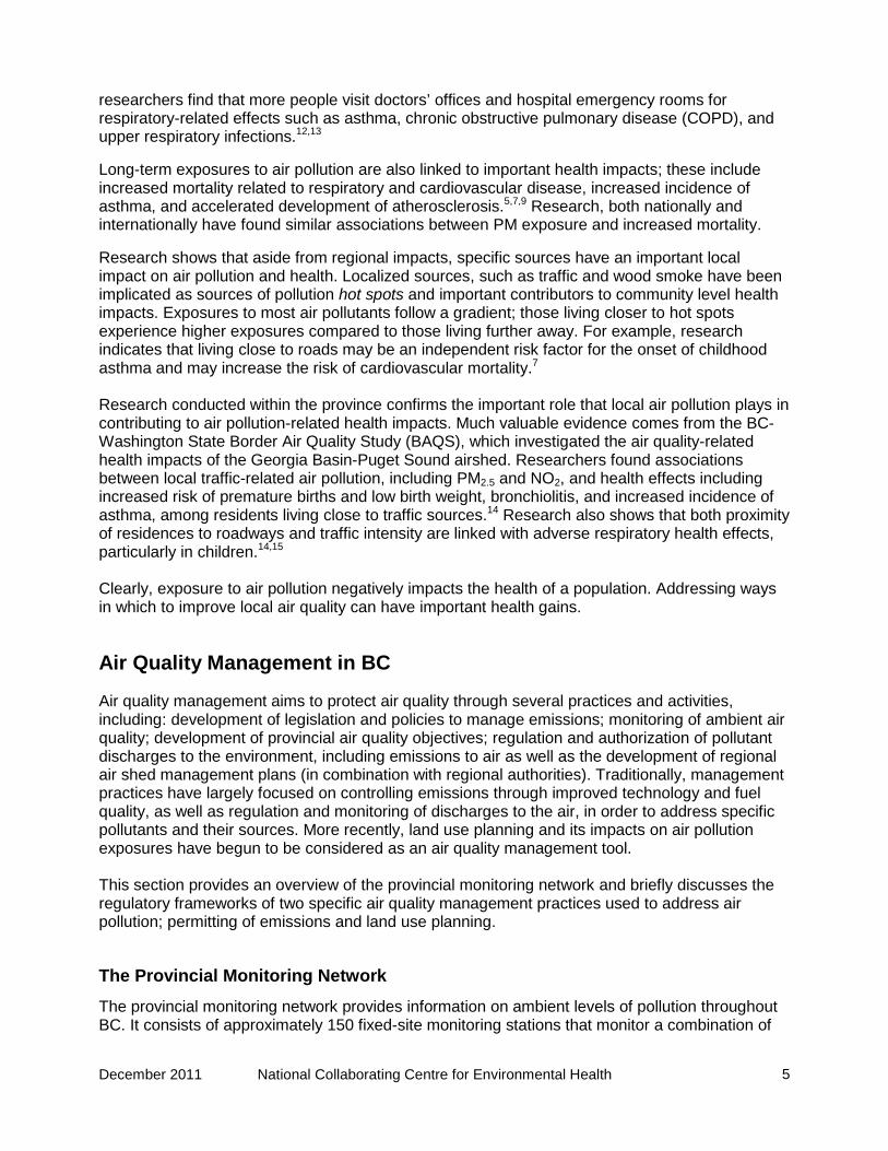
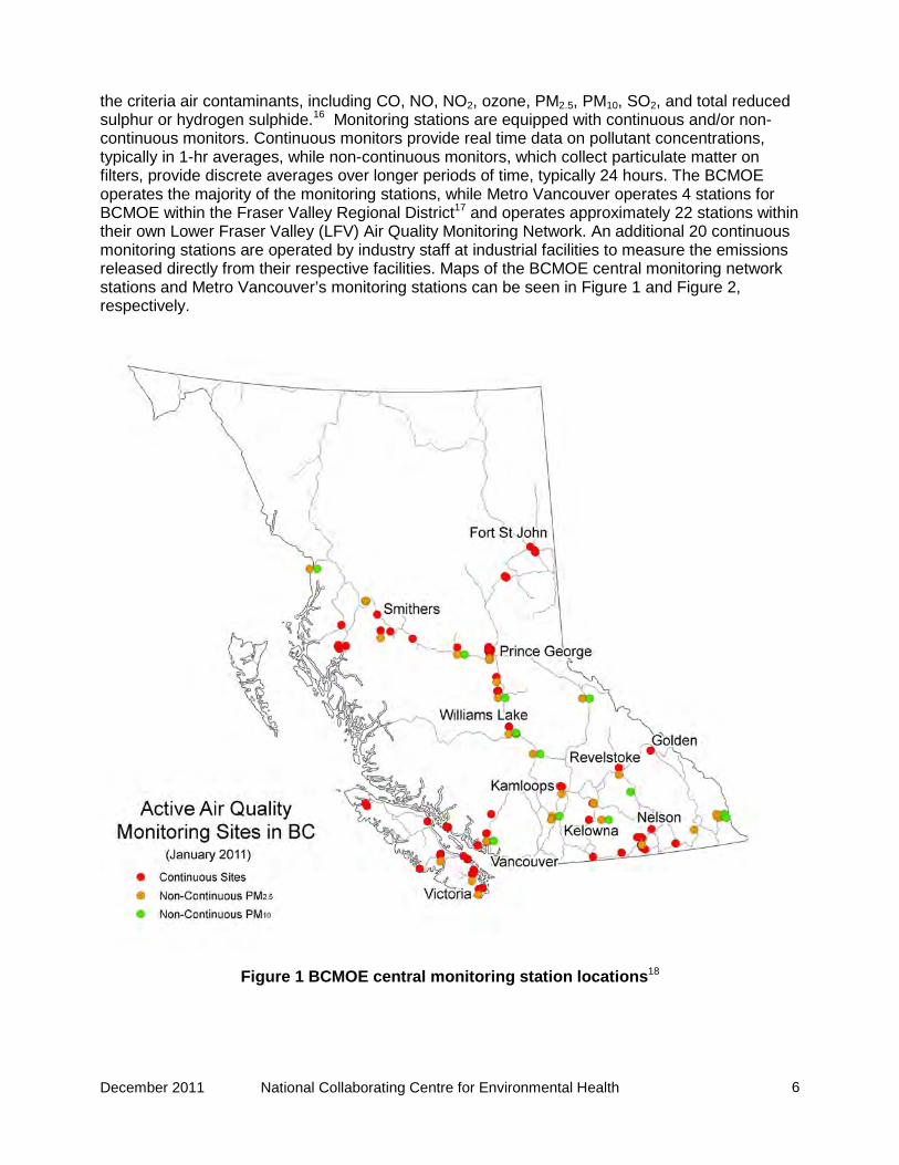
the criteria air contaminants, including CO, NO, NO2, ozone, PM2.5, PM10, SO2, and total reduced sulphur or hydrogen sulphide.16 Monitoring stations are equipped with continuous and/or non-continuous monitors. Continuous monitors provide real time data on pollutant concentrations, typically in 1-hr averages, while non-continuous monitors, which collect particulate matter on filters, provide discrete averages over longer periods of time, typically 24 hours. The BCMOE operates the majority of the monitoring stations, while Metro Vancouver operates 4 stations for BCMOE within the Fraser Valley Regional District17 and operates approximately 22 stations within their own Lower Fraser Valley (LFV) Air Quality Monitoring Network. An additional 20 continuous monitoring stations are operated by industry staff at industrial facilities to measure the emissions released directly from their respective facilities. Maps of the BCMOE central monitoring network stations and Metro Vancouver’s monitoring stations can be seen in Figure 1 and Figure 2, respectively.
Figure 1 BCMOE central monitoring station locations18
December 2011 National Collaborating Centre for Environmental Health 7
Figure 2 Metro Vancouver's monitoring station locations within the Lower Fraser Valley Air Quality Monitoring Network19
This monitoring network provides valuable information on regional air quality and in places such as Metro Vancouver, where monitor density is high, it can also provide useful information on local air quality. In places where monitors do not exist, or in communities with low monitor density, the monitoring network is limited in the information it provides, especially considering that many pollutants display high spatial and temporal variability. Originally, monitoring stations were added to the network case by case, based on monitoring needs, but more recently the BCMOE has developed a framework to ensure the network fulfills specific objectives, including ensuring compliance with the Canada Wide Standards (CWS), tracking progress with the National Ambient Air Quality Objectives (NAAQO), assessing trends, and collecting data on background levels.20
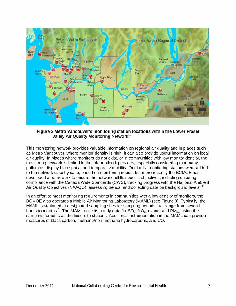
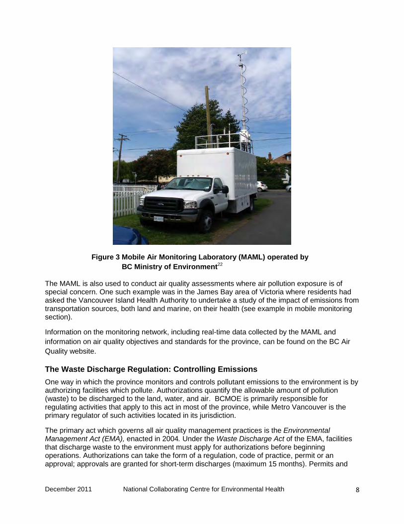
In an effort to meet monitoring requirements in communities with a low density of monitors, the BCMOE also operates a Mobile Air Monitoring Laboratory (MAML) (see Figure 3). Typically, the MAML is stationed at designated sampling sites for sampling periods that range from several hours to months.21 The MAML collects hourly data for SO2, NO2, ozone, and PM2.5 using the same instruments as the fixed-site stations. Additional instrumentation in the MAML can provide measures of black carbon, methane/non-methane hydrocarbons, and CO.
December 2011 National Collaborating Centre for Environmental Health 8
Figure 3 Mobile Air Monitoring Laboratory (MAML) operated by BC Ministry of Environment22 The MAML is also used to conduct air quality assessments where air pollution exposure is of special concern. One such example was in the James Bay area of Victoria where residents had asked the Vancouver Island Health Authority to undertake a study of the impact of emissions from transportation sources, both land and marine, on their health (see example in mobile monitoring section).
Information on the monitoring network, including real-time data collected by the MAML and information on air quality objectives and standards for the province, can be found on the BC Air Quality website.
The Waste Discharge Regulation: Controlling Emissions One way in which the province monitors and controls pollutant emissions to the environment is by authorizing facilities which pollute. Authorizations quantify the allowable amount of pollution (waste) to be discharged to the land, water, and air. BCMOE is primarily responsible for regulating activities that apply to this act in most of the province, while Metro Vancouver is the primary regulator of such activities located in its jurisdiction.
The primary act which governs all air quality management practices is the Environmental Management Act (EMA), enacted in 2004. Under the Waste Discharge Act of the EMA, facilities that discharge waste to the environment must apply for authorizations before beginning operations. Authorizations can take the form of a regulation, code of practice, permit or an approval; approvals are granted for short-term discharges (maximum 15 months). Permits and
December 2011 National Collaborating Centre for Environmental Health 9
approvals limit the quantity and types of pollutants emitted, require reporting of emissions, and where deemed necessary, may require monitoring to be conducted by the facility.
In order to issue an authorization, the BCMOE (or Metro Vancouver) typically require information on proposed criteria air contaminant emissions including maximum concentrations and total flow volumes form all stacks; information about additional pollutants may also be required, depending on the type of facility. The maximum emissions then become the never exceed stack criteria for compliance purposes. These stack criteria are negotiated between the facility and the regulator and generally strive to attain the lowest practical emission limits, based on the specific processes and available control equipment at the facility. Stack monitoring, as well as sampling and reporting requirements, are detailed in the authorization and results are sent to the regional office. Larger facilities, such as pulp mills and smelters, are typically required to establish an ambient monitoring program; specific details are left to side agreements between the regional office and the facility. Prior to applying for a permit from BCMOE or Metro Vancouver, facilities undergoing an expansion of production (i.e., amendment), may be required to undergo an assessment by BC Environmental Assessment Office and any facility located on federal lands or jurisdictions may require an assessment under the Canadian Environmental Assessment Act. Applicants of most new authorizations and amendments must also conduct public notification (e.g., newspaper notices); the level is determined by the regional office during the application process. Although the EMA allows for a number of options for authorizing discharges of waste into the environment, permits are currently the most common form of authorization. Although the permitting process allows the province to monitor pollutant emissions from important local sources, there are limitations. The never exceed values for compliance purposes may not necessarily consider other sources and emissions in the airshed. Since permits are renewed only when a facility changes their emissions output, there is no incentive for facilities to lower their emissions once a permit is issued. The permit process is based on a system of annual fees to be paid to BCMOE or Metro Vancouver, depending on the quantity of contaminants emitted to the environment. In theory, this system is intended to provide an incentive to facilities to reduce their emissions to levels as low as possible. However, in practice, due to the limits of technology, fees have been based on the permit stack criteria and thus are static until the facility changes the contaminant concentrations in their permits. Additionally, although the enactment of the EMA has helped to standardize emissions permitting decisions in the province, inconsistencies in permits issued prior to EMA still persist. The most notable inconsistency is reflected in air quality monitoring requirements, which can differ for similar facilities. With this in mind the BCMOE has set, as one its priorities, replacing permits with codes of practice wherever possible.
Land Use Planning: The Regulatory Framework
Local air quality is influenced by the sources and activities in an area, including: levels and types of transportation, industry, land use and development activities. With the exception of ozone, pollutant concentrations tend to be most elevated at the source site and decrease with increasing distance from the source. Therefore, the way that land is used and where sources are cited, relative to populations, is critical to addressing and reducing air pollution-related health impacts. In BC, land use planning and regulation is primarily a municipal responsibility, although federal and First Nations levels of government can be involved when land use decisions overlap with their respective jurisdictions. The primary law governing regional and municipal land use planning is the BC Local Government Act, 23 which is administered by the Ministry of Community and Rural
December 2011 National Collaborating Centre for Environmental Health 10
Development (formerly the Ministry of Municipal Affairs and Housing).24 The Local Government Act provides local governments with the authority to develop regional growth strategies which promote environmentally healthy human settlements through efficient use of public facilities, services, and land. The Act further enables local governments to divide land into zones, and to “regulate use, density, and aspects of buildings and structures within these zones.”24 This allows local governments to avoid or limit incompatible land uses (such as, heavy industry next to a residential area). The Community Charter provides municipalities with a range of bylaw-making powers. In areas of overlapping or concurrent authority with the province, specifically related to public health, municipalities still have the power to develop their own bylaws, but are subject to participation by the province. Such areas include protection of the natural environment, wildlife, building standards, and prohibition of soil deposit or removal.24
The establishment of local bylaws is an important way in which municipal governments can address local air quality. Several municipalities have instituted bylaws that address idling, wood burning appliance technologies, and open burning, to reduce important sources of local air pollution.25 Setbacks, or minimum distances between sources and receptors, are used to separate people from pollution sources. In BC, setback distances of 150 m between major roadways and residences are recognized as important for reducing respiratory health impacts among the public. Developers, including those who design, build or approve developments, also play an important role in addressing health impacts of land use and development. To help guide urban and rural land development in a way that takes health into account, including air quality related health impacts, the BCMOE has assembled a number of best practices in its Develop with Care guidelines.26 This document is intended for those who are responsible for development and for those who design, build or approve developments. Recommended best practices include air quality goals in community plans, developing bylaws to protect local air quality, and providing setbacks from major transportation routes for sensitive land uses, such as schools and hospitals.
Communicating Health Messages
Messages on air quality-related health impacts are delivered to the public through various channels in BC. During short-term events of poor outdoor air quality, such as forest fires, air quality advisories may be issued by regional health authorities to inform the public about deteriorated outdoor air quality. Information on regional air quality is available to the public through the Air Quality Health Index (AQHI), in an on-line format. In case of emergencies, such as chemical spills and fires that impact air quality and pose serious health concerns, provincial, regional, and local authorities work together to ensure that public health and safety is protected. Air quality advisories, the AQHI, and messages provided during emergency situations inform the public about short-term exposures; advisories, the AQHI, as well as other sources of information are discussed briefly below. No formal procedure exists to inform the public about chronic health impacts of long-term exposures to air pollution.
Air Quality Advisories
Air quality advisories provide information and advice to the public during short-term periods of poor outdoor air quality in a specific area. Advisories are typically issued when a pollutant approaches or exceeds a predetermined trigger value, typically a guideline or standard. The purpose of an advisory is to inform the public about mandatory and voluntary actions to reduce or prevent further emissions, as well as to provide messages about potential health risks and advise
December 2011 National Collaborating Centre for Environmental Health 11
about protective measures, while the advisory is in effect. The BCMOE, Metro Vancouver (for events within the Greater Vancouver Regional District), and Regional Health Authorities (RHAs) are responsible for issuing advisories. In many parts of BC, BCMOE and RHAs have worked with the Ministry of Health Services (formerly the Ministry of Healthy Living and Sport) and the British Columbia Centre for Disease Control to develop advisory templates and jointly issue air quality advisories; these templates were developed to promote greater consistency in format and content across the province. In British Columbia, advisories are issued for:
• fine particles (when PM2.5 levels exceed 25 µg/m3 over 24 hours); • ozone (when levels exceed 82 ppb over 1 hour); • dust (when PM10 levels exceed 50 µg/m3 over 24 hours); • wildfire smoke (when information, such as PM2.5 levels, presence of a visible plume, or
meteorological conditions, indicates the need to issue an advisory). Examples of advisories in BC, as well as across Canada, are summarized in An Introduction to Air Quality Advisories by the National Collaborating Centre for Environmental Health.
Air Quality Health Index
The AQHI is a tool developed by Health Canada to provide information on regional air quality to the public. The objective of the AQHI is to increase public awareness of air quality issues within the region so individuals can make behavioural changes that can result in reduced personal exposure. Daily AQHI readings are based on measurements or forward estimates of three pollutant concentrations; nitrogen dioxide, ozone, and PM2.5 are multiplied by coefficients reflecting the risk of ill health, over the short-term for each pollutant in the region. An hourly AQHI reading (0 to +10) is assigned to a region, and is categorized into a good, fair or poor reading, along with accompanying health messages. See the Air Quality Health Index website for more information.
Since the AQHI is meant to reflect the aggregate impact of air pollution exposure, readings are based on concentrations of all three pollutants. Analysis of the Canadian big city daily mortality records, used in the development of the AQHI, showed a stronger association between unit increase of NO2 and mortality, as compared to other pollutants.27 As a result, NO2 is weighted most heavily in the AQHI equation, followed by ozone, and PM. One concern that has been raised with its use in BC is that the AQHI may not accurately reflect regional air quality in many cases within the province because of this weighting. In many areas of BC, elevated levels of PM2.5 may exist without concurrent elevations in NO2 and ozone. Therefore, a good reading may be reported even when air quality is deteriorated due to elevated PM.
Other Sources of Information
BCMOE makes several air quality related reports available on the BC Air Quality website. Included are reports to summarize air quality assessments in specific communities, information on airshed planning, as well as reports on specific pollutants in BC. Several of these reports specifically address the health impacts of air quality in the province. The BC Lung Association also publishes an annual report, the State of the Air Report, to describe air quality across the province, to provide information on important pollutants, and to summarize actions across BC to address air quality issues.
December 2011 National Collaborating Centre for Environmental Health 12
Air Quality Assessment Tools Air quality assessment tools can help provide information on important sources, emissions, as well as meteorological conditions that contribute to poor local air quality. Each of the five air quality assessment tools discussed in this section will provide an introduction to the information they provide, as well as examples of their use in BC.
1. Emissions Inventories
Introduction Emissions inventories are databases of pollution sources located within a specific geographical area, along with their estimated or actual emissions. Emissions inventories may include data on specific emissions generated throughout the country, a province, or a region. The pollutants included in inventories generally include the CAC pollutants, such as PM (PM2.5 and PM10), SOx, NOx, VOCs, CO, NH3, and ozone. Data on greenhouse gas (GHG) emissions or toxics, including heavy metals, may also be included in inventories, although they are developed with different estimation methods.
Inventory Development Sources of emissions are organized into stationary and mobile categories, with stationary sources further broken down into point and area sources. Point sources include larger facilities, such as pulp mills, smelters, power plants, and wood products plants, which require authorization from the BCMOE (or Metro Vancouver). Area sources are stationary sources that are too small and numerous to count individually; these are typically associated with urban activities, such as space heating, small businesses, and restaurants. Area sources can also include activities, such as backyard and open burning, as well as farming. Mobile sources include any sources powered by an internal combustion engine that move under their own power; these include all on-road vehicles (i.e., any licensed vehicle), off-road vehicles (e.g., construction equipment, sports equipment, gardening equipment), aircraft (usually confined to the area in and around airports), marine vessels (usually confined to some distance from shore), and rail equipment. Natural sources, such as growing vegetation, windblown dust, wildfires and volcanoes can also be included in inventory preparation.
Pollutant emissions from each source are calculated using a variety of data. For point sources, data generally come from stack sampling and monitoring, as required of larger facilities by the permitting process. For point sources where stack monitoring data is not available, such as smaller facilities that are not required to conduct monitoring, estimation methods are used to calculate emissions rates of pollutants. The use of monitoring data allows for more accurate calculations of emissions from facilities, compared with those generated by estimation methods. These methods typically include the use of emission factors and a production or activity level. For many common industrial processes and control equipment, an existing emission factor can be found for similar facilities. For example, the United States Environmental Protection Agency (US EPA) maintains a large database of these factors, called the AP-42 Emission Factors.28 Emission factors are usually expressed as a mass of contaminant emitted per unit of input energy or raw material consumed (called the activity level). Once the emission factor and activity rate are known, the overall emissions from a source or activity can be calculated using equation 1.28
December 2011 National Collaborating Centre for Environmental Health 13
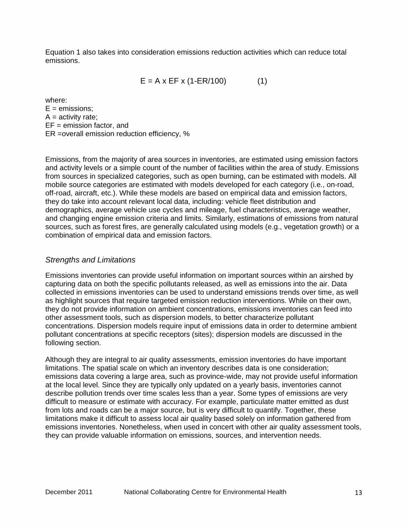
Equation 1 also takes into consideration emissions reduction activities which can reduce total emissions.
E = A x EF x (1-ER/100) (1)
where: E = emissions; A = activity rate; EF = emission factor, and ER =overall emission reduction efficiency, %
Emissions, from the majority of area sources in inventories, are estimated using emission factors and activity levels or a simple count of the number of facilities within the area of study. Emissions from sources in specialized categories, such as open burning, can be estimated with models. All mobile source categories are estimated with models developed for each category (i.e., on-road, off-road, aircraft, etc.). While these models are based on empirical data and emission factors, they do take into account relevant local data, including: vehicle fleet distribution and demographics, average vehicle use cycles and mileage, fuel characteristics, average weather, and changing engine emission criteria and limits. Similarly, estimations of emissions from natural sources, such as forest fires, are generally calculated using models (e.g., vegetation growth) or a combination of empirical data and emission factors.
Strengths and Limitations
Emissions inventories can provide useful information on important sources within an airshed by capturing data on both the specific pollutants released, as well as emissions into the air. Data collected in emissions inventories can be used to understand emissions trends over time, as well as highlight sources that require targeted emission reduction interventions. While on their own, they do not provide information on ambient concentrations, emissions inventories can feed into other assessment tools, such as dispersion models, to better characterize pollutant concentrations. Dispersion models require input of emissions data in order to determine ambient pollutant concentrations at specific receptors (sites); dispersion models are discussed in the following section.
Although they are integral to air quality assessments, emission inventories do have important limitations. The spatial scale on which an inventory describes data is one consideration; emissions data covering a large area, such as province-wide, may not provide useful information at the local level. Since they are typically only updated on a yearly basis, inventories cannot describe pollution trends over time scales less than a year. Some types of emissions are very difficult to measure or estimate with accuracy. For example, particulate matter emitted as dust from lots and roads can be a major source, but is very difficult to quantify. Together, these limitations make it difficult to assess local air quality based solely on information gathered from emissions inventories. Nonetheless, when used in concert with other air quality assessment tools, they can provide valuable information on emissions, sources, and intervention needs.
December 2011 National Collaborating Centre for Environmental Health 14
Example 1 Canada’s National Emissions Inventory
The National Pollutant Release Inventory (NPRI), produced by Environment Canada, is an example of a nationally legislated emissions inventory.29 The NPRI collects information on pollutant releases to air, water, and land, as well as on waste transfer (for disposal or recycling) across Canada. Data collected by the NPRI includes emissions of over 300 reportable pollutants released into the environment by facilities, as well as estimates for emissions from motor vehicles, residential heating and natural sources, including forest fires and open burning. Facility emissions data is updated annually, with a 1-2 year lag in the most current data. Area and mobile data is updated less frequently.
Every year, the NPRI reporting requirements are published in the Canada Gazette notice.30 Facilities which meet the requirements must report on emissions of reportable substances to Environment Canada, as mandated by the Canadian Environmental Protection Act 1999. The list of reportable substances and their threshold values for reporting can be found on the NPRI website. If one or more of these substances is manufactured, processed or used at the facility during the reporting year, in an amount that meets or exceeds the threshold value, the facility must report the amount emitted to air, water, and land. Reporting requirements have changed since the NRPI was first developed in 1993; typical changes include the addition of reportable substances, a decrease or increase in threshold values for which reporting is required, and the removal of exemptions for specific facilities or activities. Summary reports are generated annually by Environment Canada, which in turn inform priority areas for national, provincial/territorial, and regional air quality management, including the development of regulations. The NPRI is used to assess Canada’s compliance with domestic and international standards and guidelines; also has provincial applications. As with any emissions inventory, the information gathered by the NPRI is limited. Facilities use different methods to estimate emissions data which limits comparability between facilities and not all emissions are captured. Additionally, while the NPRI provides useful data on emissions generated in Canada, it does not capture information on trans-boundary emissions, which also impact local and regional air quality.
Example 2 BC’s Provincial CAC Emission Inventory The province maintains an emissions inventory on Criteria Air Contaminants (CAC) which is updated on a five-year cycle. Summary reports provide information on the major contributors in the province by area, sector, and pollutant. Such information is used in both provincial and regional air quality management to better target industries and pollutants.
The methods used to develop the CAC inventory have changed in recent years. The primary data sources for the 2005 inventory were the NPRI database as well as the BCMOE permit and fee database; previously in 2000, most of the data for the CAC inventory was generated through a survey of permit holders in the province. The reliance on permit holder and NPRI databases for inventory development has important limitations. As the Ministry of Health Services (formerly the Ministry of Healthy Living and Sport) notes in the 2005 CAC emissions inventory summary report, the province’s permitting process does not capture emissions from fugitive sources, small stacks, vents, and building ventilation.2 Additionally inconsistencies within the permitting process, including differences in monitoring requirements of similar facilities, can lead to further limitations of the data. Additionally, the NPRI may not provide comprehensive information on important emitters within the province. For example, while data on total reduced sulphur (TRS) is included
December 2011 National Collaborating Centre for Environmental Health 15
in the 2005 provincial inventory, one of the two sources of information, the NPRI, does not require reporting of TRS. Consequently, pollution emissions from important sources, such as the BC oil and gas industry,31 may not be captured by either the provincial or national inventory. Nonetheless, this provincial inventory does provide valuable information for many activities in air quality management understanding of annual trends in the province, highlights important emissions and sources, and informs other assessment activities, such as dispersion modeling.
The province also compiles inventories which focus on specific sector emissions. These include inventories related to wood-fired combustion equipment and residential wood burning, all of which can be found on the Emissions Inventories section of the BC Air Quality website.
Example 3 Metro Vancouver’s Regional Emissions Inventory
Metro Vancouver staff prepares a regional scale emissions inventory to support their Air Quality Management Plan. This inventory compiles emissions data on CAC and greenhouse gases (carbon dioxide, methane, and nitrous oxide) on a five year cycle from point, area, and mobile sources. Emissions released within the Lower Fraser Valley (LFV) international airshed, which includes the Greater Vancouver Regional District, the south-western portion of the Fraser Valley Regional District, and Whatcom Country, Washington State, are compiled in the inventories.3
Once data are collected for a given cycle, forecasts and backcasts of general emissions trends are prepared. Forecasts predict future emissions based on projected/proposed changes in activity or source, as well as changes in emission rates due to reduction measures or controls. Backcasts of older data are also conducted, using the most current methods. The use of backcasts allows for comparisons between recent and older data sets; comparing results of an inventory developed in the present with those done 5, 10, or 15 years earlier could prevent inaccurate conclusions, since apparent differences could be due to changes in estimation methods. By highlighting important current and future sources of pollution, Metro Vancouver is able to target important sources to improve regional and local air quality. Emissions trends can highlight specific pollutants or sources that lead to deteriorated air quality and detrimental health impacts. Analysis of emissions data additionally provides evidence of successful initiatives, such as AirCare,32 a vehicle emissions testing program which is credited to reducing NOx emissions in the Greater Vancouver region. The use of forecasts is especially important to long-term air quality management plans by Metro Vancouver. Forecasts are used to indicate Metro Vancouver’s ability to meet future emissions reductions goals, including the BC Government’s GHG reduction targets for 2030, highlighting any areas where action is needed.
2. Dispersion Modelling
Introduction
When a pollutant is emitted into the air, it is transported and diluted by the atmosphere and may be transformed or removed before it reaches a receptor (site). It is often assumed that air quality is determined only by how much is emitted into the air. While the amounts emitted into the air are very important to monitor, ambient concentrations are also a function of meteorology, topography, time, and the distance between sources and receptors. Because of this, the ambient concentrations are not related in a simple way to the emission amount. Dispersion models take
December 2011 National Collaborating Centre for Environmental Health 16
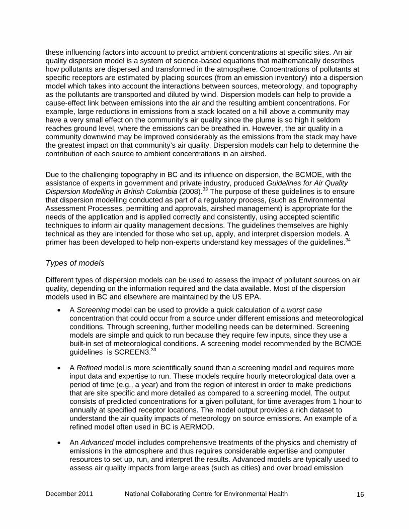
these influencing factors into account to predict ambient concentrations at specific sites. An air quality dispersion model is a system of science-based equations that mathematically describes how pollutants are dispersed and transformed in the atmosphere. Concentrations of pollutants at specific receptors are estimated by placing sources (from an emission inventory) into a dispersion model which takes into account the interactions between sources, meteorology, and topography as the pollutants are transported and diluted by wind. Dispersion models can help to provide a cause-effect link between emissions into the air and the resulting ambient concentrations. For example, large reductions in emissions from a stack located on a hill above a community may have a very small effect on the community’s air quality since the plume is so high it seldom reaches ground level, where the emissions can be breathed in. However, the air quality in a community downwind may be improved considerably as the emissions from the stack may have the greatest impact on that community’s air quality. Dispersion models can help to determine the contribution of each source to ambient concentrations in an airshed.
Due to the challenging topography in BC and its influence on dispersion, the BCMOE, with the assistance of experts in government and private industry, produced Guidelines for Air Quality Dispersion Modelling in British Columbia (2008).33 The purpose of these guidelines is to ensure that dispersion modelling conducted as part of a regulatory process, (such as Environmental Assessment Processes, permitting and approvals, airshed management) is appropriate for the needs of the application and is applied correctly and consistently, using accepted scientific techniques to inform air quality management decisions. The guidelines themselves are highly technical as they are intended for those who set up, apply, and interpret dispersion models. A primer has been developed to help non-experts understand key messages of the guidelines.34
Types of models
Different types of dispersion models can be used to assess the impact of pollutant sources on air quality, depending on the information required and the data available. Most of the dispersion models used in BC and elsewhere are maintained by the US EPA.
• A Screening model can be used to provide a quick calculation of a worst case concentration that could occur from a source under different emissions and meteorological conditions. Through screening, further modelling needs can be determined. Screening models are simple and quick to run because they require few inputs, since they use a built-in set of meteorological conditions. A screening model recommended by the BCMOE guidelines is SCREEN3.33
• A Refined model is more scientifically sound than a screening model and requires more input data and expertise to run. These models require hourly meteorological data over a period of time (e.g., a year) and from the region of interest in order to make predictions that are site specific and more detailed as compared to a screening model. The output consists of predicted concentrations for a given pollutant, for time averages from 1 hour to annually at specified receptor locations. The model output provides a rich dataset to understand the air quality impacts of meteorology on source emissions. An example of a refined model often used in BC is AERMOD.
• An Advanced model includes comprehensive treatments of the physics and chemistry of emissions in the atmosphere and thus requires considerable expertise and computer resources to set up, run, and interpret the results. Advanced models are typically used to assess air quality impacts from large areas (such as cities) and over broad emission
December 2011 National Collaborating Centre for Environmental Health 17
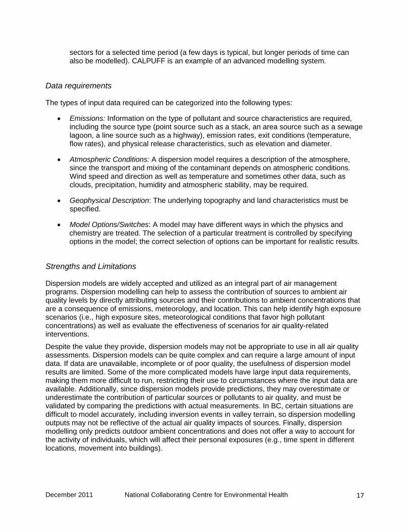
sectors for a selected time period (a few days is typical, but longer periods of time can also be modelled). CALPUFF is an example of an advanced modelling system.
Data requirements
The types of input data required can be categorized into the following types:
• Emissions: Information on the type of pollutant and source characteristics are required, including the source type (point source such as a stack, an area source such as a sewage lagoon, a line source such as a highway), emission rates, exit conditions (temperature, flow rates), and physical release characteristics, such as elevation and diameter.
• Atmospheric Conditions: A dispersion model requires a description of the atmosphere, since the transport and mixing of the contaminant depends on atmospheric conditions. Wind speed and direction as well as temperature and sometimes other data, such as clouds, precipitation, humidity and atmospheric stability, may be required.
• Geophysical Description: The underlying topography and land characteristics must be specified.
• Model Options/Switches: A model may have different ways in which the physics and chemistry are treated. The selection of a particular treatment is controlled by specifying options in the model; the correct selection of options can be important for realistic results.
Strengths and Limitations
Dispersion models are widely accepted and utilized as an integral part of air management programs. Dispersion modelling can help to assess the contribution of sources to ambient air quality levels by directly attributing sources and their contributions to ambient concentrations that are a consequence of emissions, meteorology, and location. This can help identify high exposure scenarios (i.e., high exposure sites, meteorological conditions that favor high pollutant concentrations) as well as evaluate the effectiveness of scenarios for air quality-related interventions. Despite the value they provide, dispersion models may not be appropriate to use in all air quality assessments. Dispersion models can be quite complex and can require a large amount of input data. If data are unavailable, incomplete or of poor quality, the usefulness of dispersion model results are limited. Some of the more complicated models have large input data requirements, making them more difficult to run, restricting their use to circumstances where the input data are available. Additionally, since dispersion models provide predictions, they may overestimate or underestimate the contribution of particular sources or pollutants to air quality, and must be validated by comparing the predictions with actual measurements. In BC, certain situations are difficult to model accurately, including inversion events in valley terrain, so dispersion modelling outputs may not be reflective of the actual air quality impacts of sources. Finally, dispersion modelling only predicts outdoor ambient concentrations and does not offer a way to account for the activity of individuals, which will affect their personal exposures (e.g., time spent in different locations, movement into buildings).
December 2011 National Collaborating Centre for Environmental Health 18
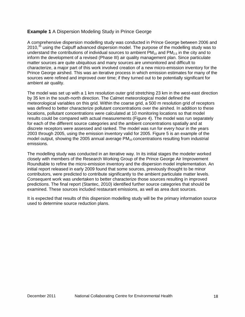
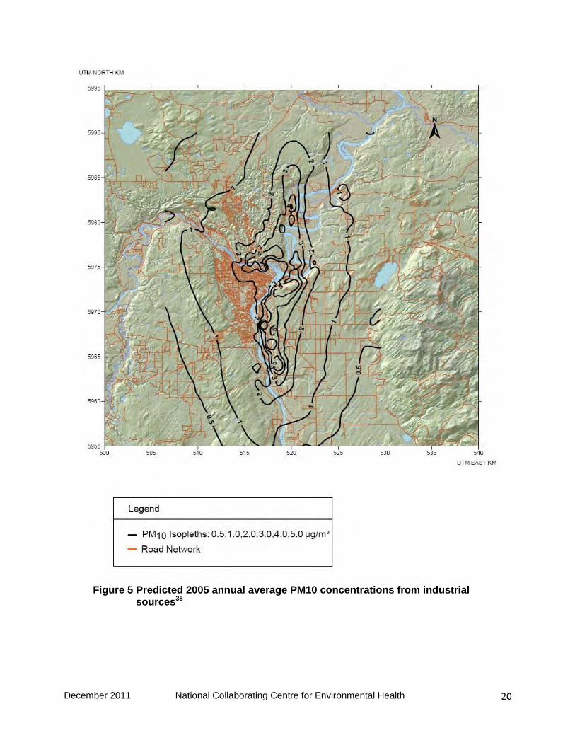
Example 1 A Dispersion Modeling Study in Prince George A comprehensive dispersion modelling study was conducted in Prince George between 2006 and 2010,35 using the Calpuff advanced dispersion model. The purpose of the modelling study was to understand the contributions of individual sources to ambient PM10 and PM2.5 in the city and to inform the development of a revised (Phase III) air quality management plan. Since particulate matter sources are quite ubiquitous and many sources are unmonitored and difficult to characterize, a major part of this work involved creation of a new micro-emission inventory for the Prince George airshed. This was an iterative process in which emission estimates for many of the sources were refined and improved over time; if they turned out to be potentially significant for ambient air quality. The model was set up with a 1 km resolution outer grid stretching 23 km in the west-east direction by 35 km in the south-north direction. The Calmet meteorological model defined the meteorological variables on this grid. Within the coarse grid, a 500 m resolution grid of receptors was defined to better characterize pollutant concentrations over the airshed. In addition to these locations, pollutant concentrations were calculated at 10 monitoring locations so that model results could be compared with actual measurements (Figure 4). The model was run separately for each of the different source categories and the ambient concentrations spatially and at discrete receptors were assessed and ranked. The model was run for every hour in the years 2003 through 2005, using the emission inventory valid for 2005. Figure 5 is an example of the model output, showing the 2005 annual average PM10 concentrations resulting from industrial emissions. The modelling study was conducted in an iterative way. In its initial stages the modeler worked closely with members of the Research Working Group of the Prince George Air Improvement Roundtable to refine the micro-emission inventory and the dispersion model implementation. An initial report released in early 2009 found that some sources, previously thought to be minor contributors, were predicted to contribute significantly to the ambient particulate matter levels. Consequent work was undertaken to better characterize those sources resulting in improved predictions. The final report (Stantec, 2010) identified further source categories that should be examined. These sources included restaurant emissions, as well as area dust sources.
It is expected that results of this dispersion modelling study will be the primary information source used to determine source reduction plans.
December 2011 National Collaborating Centre for Environmental Health 19
Figure 4 Calpuff grid used in the Prince George dispersion modelling study35
December 2011 National Collaborating Centre for Environmental Health 20
Figure 5 Predicted 2005 annual average PM10 concentrations from industrial sources35
December 2011 National Collaborating Centre for Environmental Health 21
Example 2 Developing a Dispersion Model in Bulkley Valley
Dispersion modelling of particulate matter was conducted for Bulkley Valley and the Lakes District (BVLD) airshed by the BCMOE in 2002. The BVLD airshed is located in central BC and includes the communities of Burns Lake, Houston, Telkwa, and Smithers. The main sources of PM in the area include smoke from woodstoves, open burning, backyard burning, beehive burners, and other industrial emissions, as well as road dust.
The primary objective of the modelling exercise was to better understand the contribution of different emission sources to the airshed. Information generated from the dispersion model used to: (1) understand the meteorological conditions that lead to poor air quality within the airshed, (2) determine sources that contribute to average and episodic air quality levels, (3) examine the air quality impacts of different emission control options (e.g., ban all woodstoves, install clean technology on industrial sources, reduce burning of forest debris by 50%), and (4) estimate the air quality concentrations to assess health risk in areas where there are no air quality measurements.
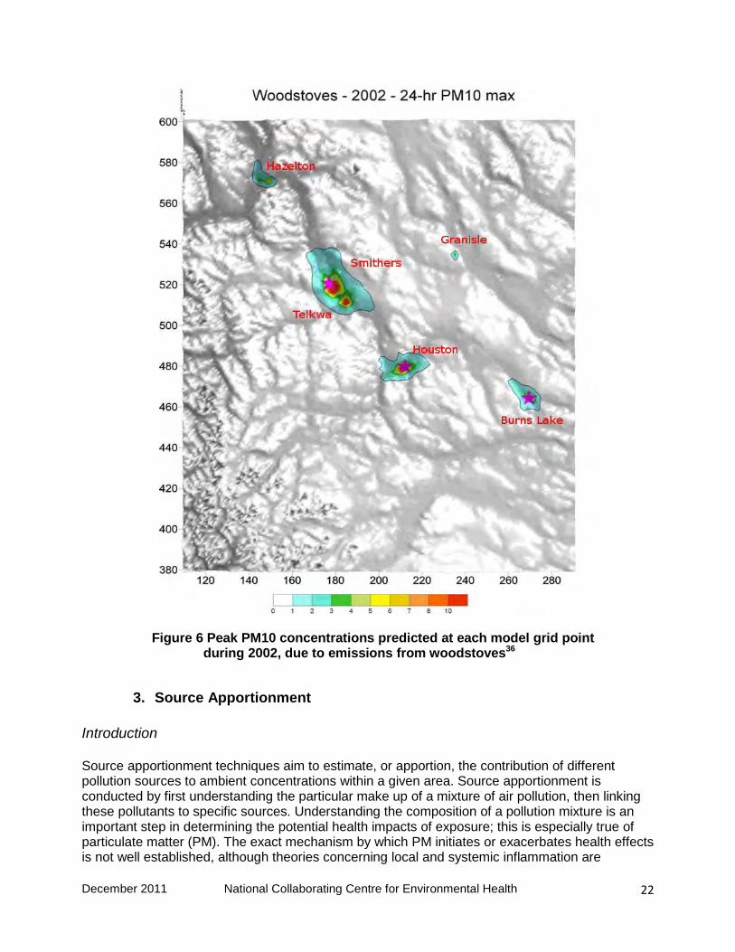
An emission inventory was first created in order to use the Calfpuff advanced dispersion model to simulate the impacts of PM emissions in the BVLD airshed on ambient air quality levels. Other model inputs included information on topography, land use, and meteorological conditions. Hourly PM10 and PM2.5 concentrations for the year 2002, within the airshed, were then predicted by the model on a 2 km resolution grid stretching 220 km from south to north and 180 km from west to east for each source. Figure 6 shows the peak PM10 concentration predicted at each model grid point, from woodstove emissions.
The model results were used to predict the impact of various management interventions on ambient air quality levels. For example, it was estimated that permanently shutting down beehive burners would reduce 24 hour average PM10 levels by as much as 1.5 μg/m3 in Burns Lake, while eliminating woodstoves would reduce 24 hour average PM10 levels by as much as 7.5 μg/m3 in Smithers. While the model was found to be realistic on most days, the emission inventory, and therefore the model output, was found to underestimate road dust and burning during spring and open burning during late fall.
Information from the dispersion modelling study was used to indicate the contribution of sources in the region to ambient air quality levels in development of the Bulkley Valley-Lakes District airshed management plan.
December 2011 National Collaborating Centre for Environmental Health 22
Figure 6 Peak PM10 concentrations predicted at each model grid point during 2002, due to emissions from woodstoves36
3. Source Apportionment Introduction Source apportionment techniques aim to estimate, or apportion, the contribution of different pollution sources to ambient concentrations within a given area. Source apportionment is conducted by first understanding the particular make up of a mixture of air pollution, then linking these pollutants to specific sources. Understanding the composition of a pollution mixture is an important step in determining the potential health impacts of exposure; this is especially true of particulate matter (PM). The exact mechanism by which PM initiates or exacerbates health effects is not well established, although theories concerning local and systemic inflammation are
December 2011 National Collaborating Centre for Environmental Health 23
becoming more accepted as plausible mechanisms.9 However, it is known that both particle size and composition can affect health. A greater understanding of particle composition, in addition to size, can also provide a better understanding of health impacts to the local population.
Types of Models
Models of varying complexity have been developed to conduct source apportionment. These models aim to attribute ambient pollutant concentrations at specific locations (receptors) to specific sources. Common models include chemical-mass balance (CMB), principle component analysis (PCA) and a related technique called positive matrix factorization (PMF). The key difference between these models is the requirement of prior knowledge/data; while CMB models rely on chemical source profiles of emission sources, as well as on the chemical composition of ambient air at receptor locations, PMF and PCA require only chemical composition information at receptors.
In order to conduct a CMB assessment for PM, filter samples are collected and undergo laboratory analysis to determine the composition of the collected samples. Additionally, the chemical profile of pollutants emitted from all major sources in the airshed must be specified. The contribution of each source to the filter chemical make-up is then calculated by combining the sources linearly. The method is improved when sources have unique chemical tracers, making it easier to match the filter PM chemical composition to a specific source.37 As very few pollutants are source-specific, only non-reactive chemical tracers may be used as indicators of specific pollutants. For example, levoglucosan, a tracer for wood smoke, is often used in the analysis of PM to apportion the contribution of wood burning to a particulate sample.
Unlike CMB, PCA and PMF models can be used when the chemical composition of emissions from potential sources are unknown. PCA and PMF are very similar; both are statistical models that use multivariate receptor analysis to identify sources of a pollutant mixture. Despite these similarities, PMF is thought to be superior to PCA for several reasons. In PMF, unlike for PCA, it is possible to account for missing data, values below the limit of detection and uncertainties in each of the data values, by assigning weights to the data values. PMF is also more realistic since negative concentrations are excluded, unlike in PCA. Using both models, the chemical constituents of a sample are analyzed and the relationships between the constituents, expressed as a covariance matrix, are investigated. When particular chemical species vary together, they are assigned to the same factor. The chemical make-up of each factor is then interpreted and identified with a specific source.37 Information from a PMF model can be further refined with the use of meteorological data, including wind direction, to provide better information on the geographical location of the source. For example, if a particular factor occurs when wind is from a specific direction, and the factor is chemically associated with a source in that direction, then the factor may be attributed to that source.
Strengths and Limitations
The use of receptor models to conduct source apportionment can provide information on the composition of local air pollution which can then be linked to specific source types. Consequently, when particular sources are identified as important contributors to local air pollution, they can be targeted for emissions reduction strategies; information about important polluters can also inform decisions on emissions permitting and industrial siting in a region. A better understanding of sources and of pollution composition can also better inform the assessment of health impacts once the exposure is better characterized.
December 2011 National Collaborating Centre for Environmental Health 24
Since many pollutants are not source specific but often have multiple sources, it can be difficult to accurately estimate the contribution of specific sources to total pollutant concentrations. Source apportionment is also resource intensive. For CMB, sometimes the chemical source profiles are not known and all important sources may not be identified. For PCA and PMF, it may be difficult to identify a factor with a specific source unless there are distinct tracers for each source.
Example 1Investigating Air Pollution Sources in Golden, Using Source Apportionment
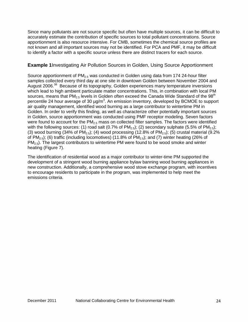
Source apportionment of PM2.5 was conducted in Golden using data from 174 24-hour filter samples collected every third day at one site in downtown Golden between November 2004 and August 2006.38 Because of its topography, Golden experiences many temperature inversions which lead to high ambient particulate matter concentrations. This, in combination with local PM sources, means that PM2.5 levels in Golden often exceed the Canada Wide Standard of the 98th percentile 24 hour average of 30 µg/m3. An emission inventory, developed by BCMOE to support air quality management, identified wood burning as a large contributor to wintertime PM in Golden. In order to verify this finding, as well as characterize other potentially important sources in Golden, source apportionment was conducted using PMF receptor modeling. Seven factors were found to account for the PM2.5 mass on collected filter samples. The factors were identified with the following sources: (1) road salt (0.7% of PM2.5); (2) secondary sulphate (5.5% of PM2.5); (3) wood burning (34% of PM2.5); (4) wood processing (12.8% of PM2.5); (5) crustal material (9.2% of PM2.5); (6) traffic (including locomotives) (11.8% of PM2.5); and (7) winter heating (26% of PM2.5). The largest contributors to wintertime PM were found to be wood smoke and winter heating (Figure 7).
The identification of residential wood as a major contributor to winter-time PM supported the development of a stringent wood burning appliance bylaw banning wood burning appliances in new construction. Additionally, a comprehensive wood stove exchange program, with incentives to encourage residents to participate in the program, was implemented to help meet the emissions criteria.
December 2011 National Collaborating Centre for Environmental Health 25
Figure 7 PMF results for Golden, BC38
Example 2 Source Apportionment in Prince George
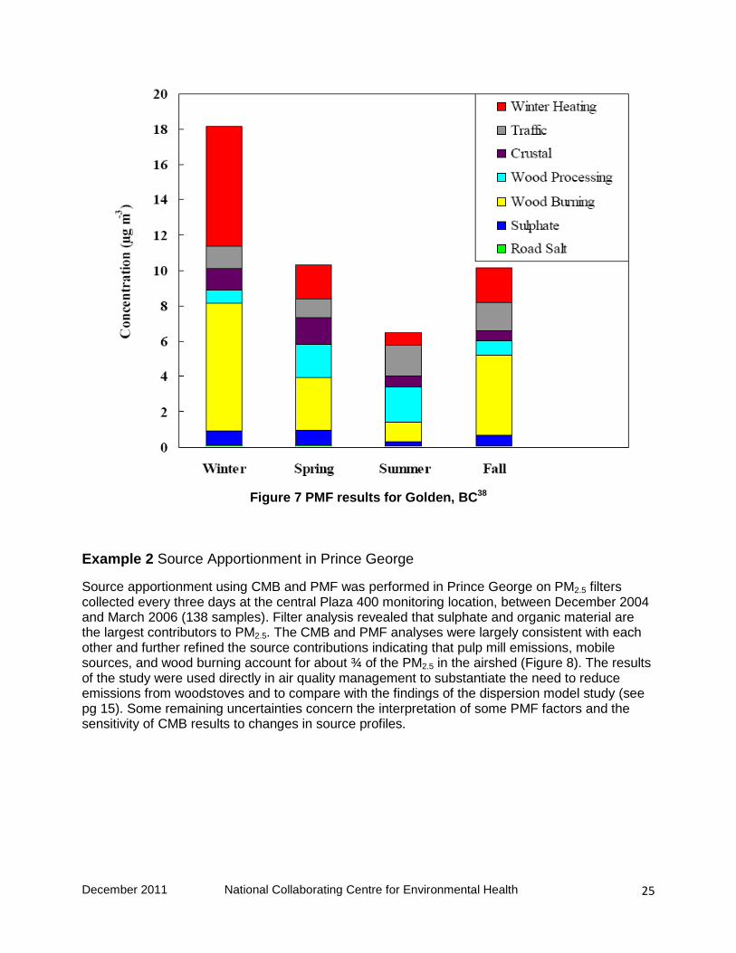
Source apportionment using CMB and PMF was performed in Prince George on PM2.5 filters collected every three days at the central Plaza 400 monitoring location, between December 2004 and March 2006 (138 samples). Filter analysis revealed that sulphate and organic material are the largest contributors to PM2.5. The CMB and PMF analyses were largely consistent with each other and further refined the source contributions indicating that pulp mill emissions, mobile sources, and wood burning account for about ¾ of the PM2.5 in the airshed (Figure 8). The results of the study were used directly in air quality management to substantiate the need to reduce emissions from woodstoves and to compare with the findings of the dispersion model study (see pg 15). Some remaining uncertainties concern the interpretation of some PMF factors and the sensitivity of CMB results to changes in source profiles.
December 2011 National Collaborating Centre for Environmental Health 26
Figure 8 Comparison of PMF and CMB source contributions averaged overall data (average), top 20% PM2.5 mass days (high mass), winter days (winter), summer days (summer) for the Prince George study39
4. Mobile Monitoring
Introduction
Mobile monitoring uses a mobile platform, typically a vehicle, to collect pollutant measurements across an area of interest. This type of monitoring is useful to: (1) provide insight about areas that are not well represented by fixed-site monitoring stations; (2) capture small-scale spatial variability of pollutants; (3) identify localized pollutant hot spots, particularly for emissions that vary in concentration over small spatial scales, such as residential wood burning and traffic; (4) provide data for model development or validation. Mobile monitoring has the capability of being rapidly deployed, therefore, can also be used in emergency situations, such as characterizing the spatial distribution of a chemical plume resulting from an accidental release or smoke from forest fires. For these reasons, mobile monitoring provides detailed information beyond what can be typically characterized by traditional fixed-site monitoring networks, so can be used to improve exposure estimates and inform air quality management decisions.
December 2011 National Collaborating Centre for Environmental Health 27
Conducting Mobile Monitoring Mobile monitoring is typically conducted by equipping a vehicle with air pollutant monitors. The use of a geographical positioning system (GPS) allows precise locations to be assigned to air pollution measurements. There are two sampling methods that can be used to conduct mobile monitoring: (1) measurements can be collected while the vehicle is in motion or (2) can be stationed for periods of time at designated locations.
Generally, the purpose of collecting measurements while the vehicle is in motion is to gather a high density of measurements over an area of interest. Continuous monitors are suitable for this approach and are typically used to collect real-time measurements at high frequencies (less than 1 minute). Several types of pollutants such as PM4 and air toxics40 have been measured, using this sampling method. Some measurements, such as PM, do not provide source-specific information, making it difficult to attribute specific sources to the mobile measurements. However, different techniques, such as choosing an appropriate sampling period or instrument selection, can help to identify or isolate the sources of interest. For example, to characterize PM2.5 generated from residential wood burning, mobile monitoring can be conducted during cold, calm winter evenings. During these conditions, wood burning activity is expected to be relatively high while the relative contribution of traffic to ambient PM2.5 is expected to be lower.4 Selecting an instrument, such as a multi-wavelength aethalometer or multi-wavelength nephelometer, instruments that measure light attenuation and scattering of a sample (respectively) at two or more wavelengths, can help to distinguish some particle sources, such as diesel exhaust or wood smoke.41 Supplementary sampling at fixed-sites can also help to characterize the chemical contents of PM2.5 within the region of interest.
In cases where sampling is conducted while the vehicle is stationary, the vehicle essentially serves as a temporary monitoring station. The vehicle is stationed at designated sampling sites in an area of interest for longer sampling periods (from hours to days). Sampling can be conducted for pollutants such as: PM, NO2, SO2, ozone, VOCs, PAHs, other air toxics, as well as for meteorological conditions with continuous and non-continuous monitors.21 This approach is useful for obtaining ambient air quality information that would otherwise not be available through existing fixed-site monitoring networks (Example 2).
Strengths and Limitations Mobile monitoring can be readily deployed and is an effective method for capturing a high resolution of measurements over an area of interest. These qualities can help to: (1) obtain more accurate exposure assessments compared to traditional fixed-site monitoring, particularly for pollutants whose concentrations have a high degree of spatial variability; (2) identify high exposure groups; (3) identify important pollutant sources that contribute to local air pollution; all of which can better inform appropriate local-scale interventions. Due to the portability of mobile monitoring, it can also serve as a screening tool to determine the need for more in-depth sampling or to site permanent monitoring stations.
Mobile monitoring is best suited for characterizing the spatial distribution of pollutants over relatively short time periods. Repeated samples are required and meteorological conditions during sampling periods need to be considered in order to provide accurate representations of exposure. Due to the labour intensive nature of mobile monitoring, it is generally not suitable for capturing temporal trends, particularly over the long-term. A second limitation of mobile monitoring is that sampling of many pollutants, including PM, may not be source specific. If the
December 2011 National Collaborating Centre for Environmental Health 28
goal is to characterize a specific pollutant source (e.g., traffic pollution or wood smoke), sampling methods must consider the sampling period, instrumentation, and use of auxiliary monitoring (e.g., fixed-site sampling) to isolate and confirm the presence of the pollutant source.
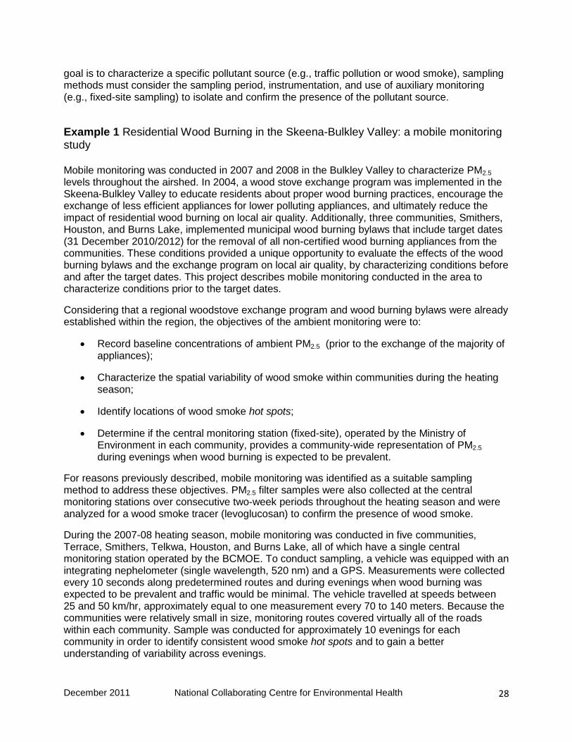
Example 1 Residential Wood Burning in the Skeena-Bulkley Valley: a mobile monitoring study Mobile monitoring was conducted in 2007 and 2008 in the Bulkley Valley to characterize PM2.5 levels throughout the airshed. In 2004, a wood stove exchange program was implemented in the Skeena-Bulkley Valley to educate residents about proper wood burning practices, encourage the exchange of less efficient appliances for lower polluting appliances, and ultimately reduce the impact of residential wood burning on local air quality. Additionally, three communities, Smithers, Houston, and Burns Lake, implemented municipal wood burning bylaws that include target dates (31 December 2010/2012) for the removal of all non-certified wood burning appliances from the communities. These conditions provided a unique opportunity to evaluate the effects of the wood burning bylaws and the exchange program on local air quality, by characterizing conditions before and after the target dates. This project describes mobile monitoring conducted in the area to characterize conditions prior to the target dates.
Considering that a regional woodstove exchange program and wood burning bylaws were already established within the region, the objectives of the ambient monitoring were to:
• Record baseline concentrations of ambient PM2.5 (prior to the exchange of the majority of appliances);
• Characterize the spatial variability of wood smoke within communities during the heating season;
• Identify locations of wood smoke hot spots;
• Determine if the central monitoring station (fixed-site), operated by the Ministry of Environment in each community, provides a community-wide representation of PM2.5 during evenings when wood burning is expected to be prevalent.
For reasons previously described, mobile monitoring was identified as a suitable sampling method to address these objectives. PM2.5 filter samples were also collected at the central monitoring stations over consecutive two-week periods throughout the heating season and were analyzed for a wood smoke tracer (levoglucosan) to confirm the presence of wood smoke.
During the 2007-08 heating season, mobile monitoring was conducted in five communities, Terrace, Smithers, Telkwa, Houston, and Burns Lake, all of which have a single central monitoring station operated by the BCMOE. To conduct sampling, a vehicle was equipped with an integrating nephelometer (single wavelength, 520 nm) and a GPS. Measurements were collected every 10 seconds along predetermined routes and during evenings when wood burning was expected to be prevalent and traffic would be minimal. The vehicle travelled at speeds between 25 and 50 km/hr, approximately equal to one measurement every 70 to 140 meters. Because the communities were relatively small in size, monitoring routes covered virtually all of the roads within each community. Sample was conducted for approximately 10 evenings for each community in order to identify consistent wood smoke hot spots and to gain a better understanding of variability across evenings.
December 2011 National Collaborating Centre for Environmental Health 29
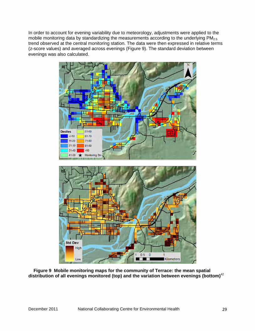
In order to account for evening variability due to meteorology, adjustments were applied to the mobile monitoring data by standardizing the measurements according to the underlying PM2.5 trend observed at the central monitoring station. The data were then expressed in relative terms (z-score values) and averaged across evenings (Figure 9). The standard deviation between evenings was also calculated.
Figure 9 Mobile monitoring maps for the community of Terrace: the mean spatial distribution of all evenings monitored (top) and the variation between evenings (bottom)42
December 2011 National Collaborating Centre for Environmental Health 30
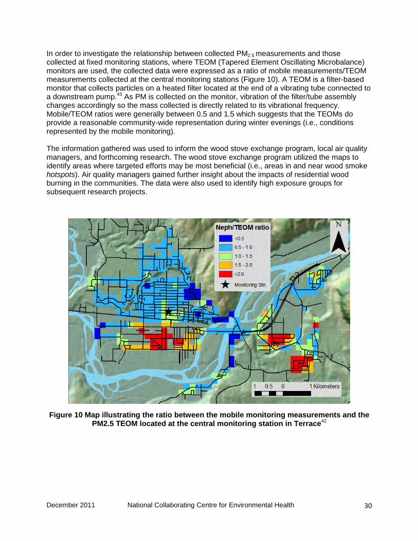
In order to investigate the relationship between collected PM2.5 measurements and those collected at fixed monitoring stations, where TEOM (Tapered Element Oscillating Microbalance) monitors are used, the collected data were expressed as a ratio of mobile measurements/TEOM measurements collected at the central monitoring stations (Figure 10). A TEOM is a filter-based monitor that collects particles on a heated filter located at the end of a vibrating tube connected to a downstream pump.43 As PM is collected on the monitor, vibration of the filter/tube assembly changes accordingly so the mass collected is directly related to its vibrational frequency. Mobile/TEOM ratios were generally between 0.5 and 1.5 which suggests that the TEOMs do provide a reasonable community-wide representation during winter evenings (i.e., conditions represented by the mobile monitoring). The information gathered was used to inform the wood stove exchange program, local air quality managers, and forthcoming research. The wood stove exchange program utilized the maps to identify areas where targeted efforts may be most beneficial (i.e., areas in and near wood smoke hotspots). Air quality managers gained further insight about the impacts of residential wood burning in the communities. The data were also used to identify high exposure groups for subsequent research projects.
Figure 10 Map illustrating the ratio between the mobile monitoring measurements and the PM2.5 TEOM located at the central monitoring station in Terrace42
December 2011 National Collaborating Centre for Environmental Health 31
Example 2 Use of the Mobile Air Monitoring Laboratory to Study Transportation Related Pollution in James Bay, Victoria As mentioned previously, in 2009 the Mobile Air Monitoring Laboratory (MAML) was used to monitor air quality in the James Bay area of Victoria, to assess the impact of emissions from transportation sources, both land and marine, on local air quality. A previous modelling study of the James Bay area indicated there could be short term peaks in SO2 levels in the neighbourhood, and these might be associated with the presence of cruise ships at the nearby terminal.44 In partnership with the BCMOE, a site that was predicted to be impacted by cruise ship emissions was found for set up of the MAML. After calibrations were conducted, continuous monitoring of SO2 (marine fuel and diesel emissions), PM2.5 (combustion, exhaust), NO, and NO2 (both associated with vehicle exhaust) was conducted over the cruise ship season from May 30 to August 24, 2009. Data were provided to researchers at the University of Victoria for analysis, after standard quality checks were performed by BCMOE staff. The data were summarized to 5-minute, hourly, and daily averages, and levels were compared to local, provincial, national, and international air quality guidelines. Data from the closest fixed-site monitor (approximately 3.5 km in distance) were also summarized to explore whether trends at the MAML site were also observable further away. Short-term peaks in the 5-minute and hourly averages for SO2 were observed in the data. Using published schedules for cruise ship arrivals and departures at the nearby Ogden Point Terminal, along with wind direction and speed data from MAML and a nearby meteorological station (Ogden Point Breakwater), researchers were able to show a correlation between cruise ship activity and these short-term peaks. Depending on meteorological conditions, short-term peaks were sometimes observed only at the MAML site or only at the fixed-site, but most often peaks were apparent at both sites. No local, provincial, or national guidelines were exceeded; however, the most recent guideline available for 24-hour average SO2 levels, recommended by the World Health Organization, was exceeded on 14 out of 87 days monitored (16 %). The Vancouver Island Health Authority provided the results to staff at the BC Centre for Disease Control for an independent health impact assessment. It was concluded that levels of SO2 could occasionally impact the health of residents who were suffering from poorly managed respiratory conditions, such as asthma. This study coincided with the development of amendments to the International Maritime Organization (IMO) MARPOL Annex VI treaty to adopt a North American Emission Control Area (ECA). The ECA will extend up to 200 nautical miles along the majority of the Canadian and U.S. coastlines and will require ships operating within this area to use fuel not exceeding 1.0 percent sulphur by 2012 and 0.1 percent sulphur by 2015. Currently, large ocean- going vessels, such as cruise ships, use fuel containing between 1.6 and 4.0 % sulphur. Future decreases in fuel sulphur content are expected to result in similar decreases in SO2 levels in local air.
5. Land Use Regression Introduction Land use regression (LUR) is a modelling approach that can be used to describe the distribution of air pollution within urban and suburban areas. It was first developed by public health researchers in the mid-1990s to examine neighbourhood-scale variability in long-term
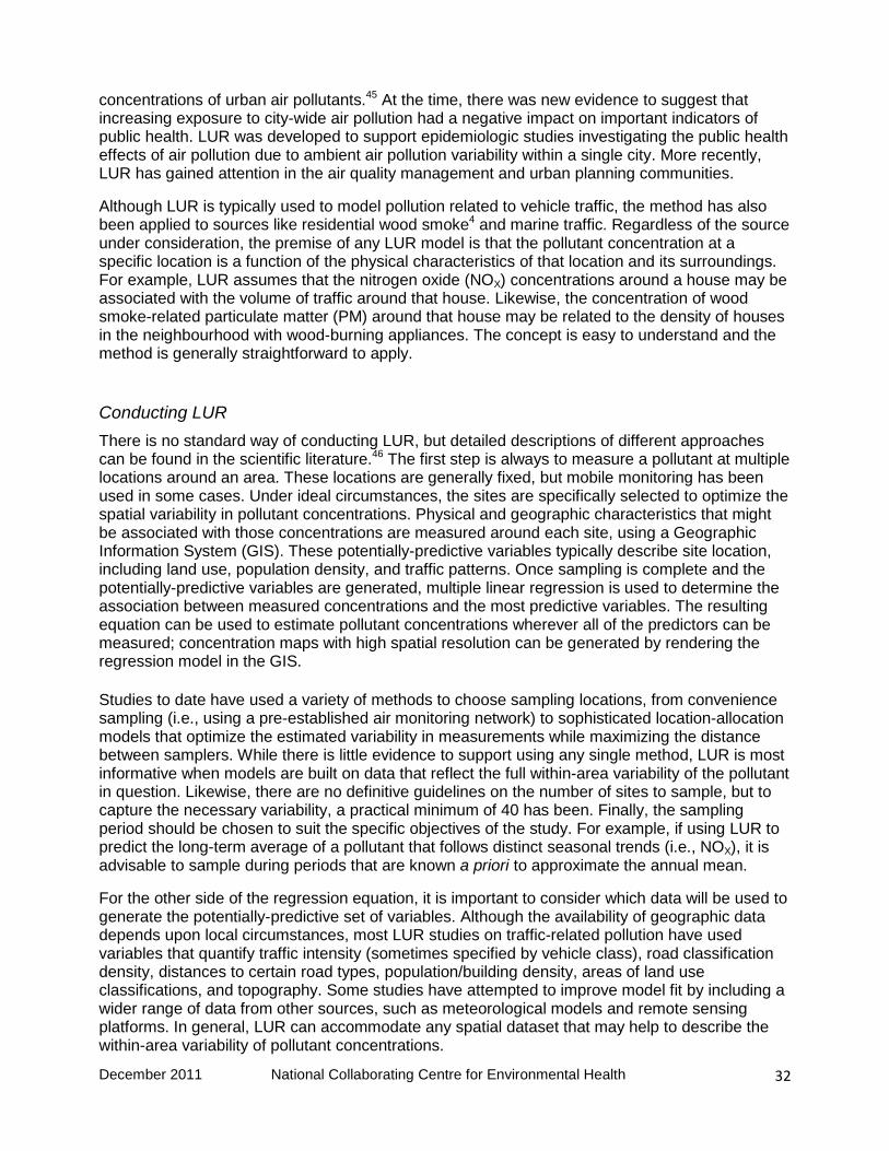
December 2011 National Collaborating Centre for Environmental Health 32
concentrations of urban air pollutants.45 At the time, there was new evidence to suggest that increasing exposure to city-wide air pollution had a negative impact on important indicators of public health. LUR was developed to support epidemiologic studies investigating the public health effects of air pollution due to ambient air pollution variability within a single city. More recently, LUR has gained attention in the air quality management and urban planning communities.
Although LUR is typically used to model pollution related to vehicle traffic, the method has also been applied to sources like residential wood smoke4 and marine traffic. Regardless of the source under consideration, the premise of any LUR model is that the pollutant concentration at a specific location is a function of the physical characteristics of that location and its surroundings. For example, LUR assumes that the nitrogen oxide (NOX) concentrations around a house may be associated with the volume of traffic around that house. Likewise, the concentration of wood smoke-related particulate matter (PM) around that house may be related to the density of houses in the neighbourhood with wood-burning appliances. The concept is easy to understand and the method is generally straightforward to apply. Conducting LUR There is no standard way of conducting LUR, but detailed descriptions of different approaches can be found in the scientific literature.46 The first step is always to measure a pollutant at multiple locations around an area. These locations are generally fixed, but mobile monitoring has been used in some cases. Under ideal circumstances, the sites are specifically selected to optimize the spatial variability in pollutant concentrations. Physical and geographic characteristics that might be associated with those concentrations are measured around each site, using a Geographic Information System (GIS). These potentially-predictive variables typically describe site location, including land use, population density, and traffic patterns. Once sampling is complete and the potentially-predictive variables are generated, multiple linear regression is used to determine the association between measured concentrations and the most predictive variables. The resulting equation can be used to estimate pollutant concentrations wherever all of the predictors can be measured; concentration maps with high spatial resolution can be generated by rendering the regression model in the GIS.
Studies to date have used a variety of methods to choose sampling locations, from convenience sampling (i.e., using a pre-established air monitoring network) to sophisticated location-allocation models that optimize the estimated variability in measurements while maximizing the distance between samplers. While there is little evidence to support using any single method, LUR is most informative when models are built on data that reflect the full within-area variability of the pollutant in question. Likewise, there are no definitive guidelines on the number of sites to sample, but to capture the necessary variability, a practical minimum of 40 has been. Finally, the sampling period should be chosen to suit the specific objectives of the study. For example, if using LUR to predict the long-term average of a pollutant that follows distinct seasonal trends (i.e., NOX), it is advisable to sample during periods that are known a priori to approximate the annual mean.
For the other side of the regression equation, it is important to consider which data will be used to generate the potentially-predictive set of variables. Although the availability of geographic data depends upon local circumstances, most LUR studies on traffic-related pollution have used variables that quantify traffic intensity (sometimes specified by vehicle class), road classification density, distances to certain road types, population/building density, areas of land use classifications, and topography. Some studies have attempted to improve model fit by including a wider range of data from other sources, such as meteorological models and remote sensing platforms. In general, LUR can accommodate any spatial dataset that may help to describe the within-area variability of pollutant concentrations.
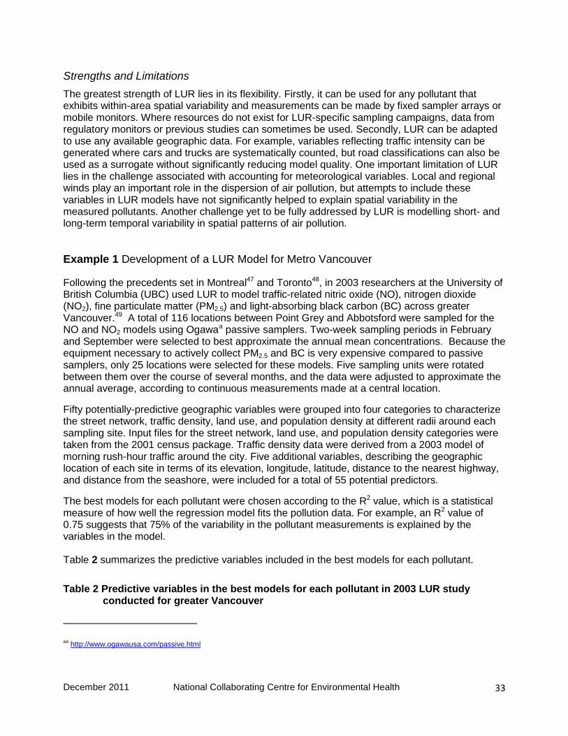
December 2011 National Collaborating Centre for Environmental Health 33
Strengths and Limitations The greatest strength of LUR lies in its flexibility. Firstly, it can be used for any pollutant that exhibits within-area spatial variability and measurements can be made by fixed sampler arrays or mobile monitors. Where resources do not exist for LUR-specific sampling campaigns, data from regulatory monitors or previous studies can sometimes be used. Secondly, LUR can be adapted to use any available geographic data. For example, variables reflecting traffic intensity can be generated where cars and trucks are systematically counted, but road classifications can also be used as a surrogate without significantly reducing model quality. One important limitation of LUR lies in the challenge associated with accounting for meteorological variables. Local and regional winds play an important role in the dispersion of air pollution, but attempts to include these variables in LUR models have not significantly helped to explain spatial variability in the measured pollutants. Another challenge yet to be fully addressed by LUR is modelling short- and long-term temporal variability in spatial patterns of air pollution. Example 1 Development of a LUR Model for Metro Vancouver
Following the precedents set in Montreal47 and Toronto48, in 2003 researchers at the University of British Columbia (UBC) used LUR to model traffic-related nitric oxide (NO), nitrogen dioxide (NO2), fine particulate matter (PM2.5) and light-absorbing black carbon (BC) across greater Vancouver.49 A total of 116 locations between Point Grey and Abbotsford were sampled for the NO and NO2 models using Ogawaa
Fifty potentially-predictive geographic variables were grouped into four categories to characterize the street network, traffic density, land use, and population density at different radii around each sampling site. Input files for the street network, land use, and population density categories were taken from the 2001 census package. Traffic density data were derived from a 2003 model of morning rush-hour traffic around the city. Five additional variables, describing the geographic location of each site in terms of its elevation, longitude, latitude, distance to the nearest highway, and distance from the seashore, were included for a total of 55 potential predictors.
passive samplers. Two-week sampling periods in February and September were selected to best approximate the annual mean concentrations. Because the equipment necessary to actively collect PM2.5 and BC is very expensive compared to passive samplers, only 25 locations were selected for these models. Five sampling units were rotated between them over the course of several months, and the data were adjusted to approximate the annual average, according to continuous measurements made at a central location.
The best models for each pollutant were chosen according to the R2 value, which is a statistical measure of how well the regression model fits the pollution data. For example, an R2 value of 0.75 suggests that 75% of the variability in the pollutant measurements is explained by the variables in the model. Table 2 summarizes the predictive variables included in the best models for each pollutant. Table 2 Predictive variables in the best models for each pollutant in 2003 LUR study
conducted for greater Vancouver
aa http://www.ogawausa.com/passive.html
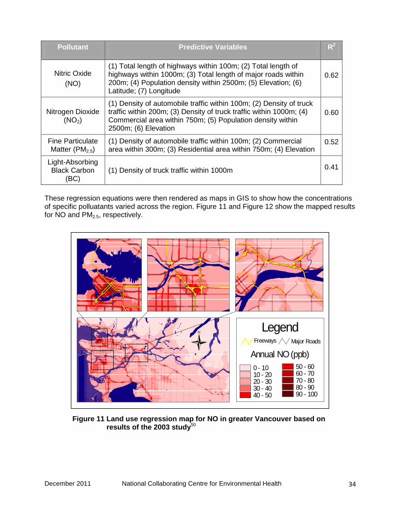
December 2011 National Collaborating Centre for Environmental Health 34
Pollutant Predictive Variables R2
Nitric Oxide (NO)
(1) Total length of highways within 100m; (2) Total length of highways within 1000m; (3) Total length of major roads within 200m; (4) Population density within 2500m; (5) Elevation; (6) Latitude; (7) Longitude
0.62
Nitrogen Dioxide (NO2)
(1) Density of automobile traffic within 100m; (2) Density of truck traffic within 200m; (3) Density of truck traffic within 1000m; (4) Commercial area within 750m; (5) Population density within 2500m; (6) Elevation
0.60
Fine Particulate Matter (PM2.5)
(1) Density of automobile traffic within 100m; (2) Commercial area within 300m; (3) Residential area within 750m; (4) Elevation
0.52
Light-Absorbing Black Carbon
(BC) (1) Density of truck traffic within 1000m 0.41
These regression equations were then rendered as maps in GIS to show how the concentrations of specific polluatants varied across the region. Figure 11 and Figure 12 show the mapped results for NO and PM2.5, respectively.
Freeways Major Roads
Legend
Annual NO (ppb)
N
0 - 1010 - 2020 - 3030 - 4040 - 50
50 - 6060 - 7070 - 8080 - 9090 - 100
Figure 11 Land use regression map for NO in greater Vancouver based on results of the 2003 study50
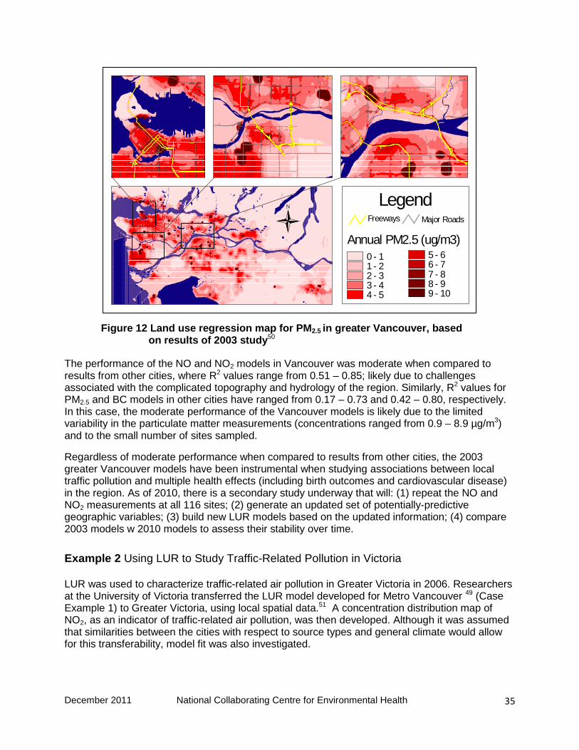
December 2011 National Collaborating Centre for Environmental Health 35
N
Annual PM2.5 (ug/m3)0 - 11 - 22 - 33 - 44 - 5
5 - 66 - 77 - 88 - 99 - 10
LegendMajor RoadsFreeways
Figure 12 Land use regression map for PM2.5 in greater Vancouver, based
on results of 2003 study50
The performance of the NO and NO2 models in Vancouver was moderate when compared to results from other cities, where R2 values range from 0.51 – 0.85; likely due to challenges associated with the complicated topography and hydrology of the region. Similarly, R2 values for PM2.5 and BC models in other cities have ranged from 0.17 – 0.73 and 0.42 – 0.80, respectively. In this case, the moderate performance of the Vancouver models is likely due to the limited variability in the particulate matter measurements (concentrations ranged from 0.9 – 8.9 µg/m3) and to the small number of sites sampled.
Regardless of moderate performance when compared to results from other cities, the 2003 greater Vancouver models have been instrumental when studying associations between local traffic pollution and multiple health effects (including birth outcomes and cardiovascular disease) in the region. As of 2010, there is a secondary study underway that will: (1) repeat the NO and NO2 measurements at all 116 sites; (2) generate an updated set of potentially-predictive geographic variables; (3) build new LUR models based on the updated information; (4) compare 2003 models w 2010 models to assess their stability over time.
Example 2 Using LUR to Study Traffic-Related Pollution in Victoria LUR was used to characterize traffic-related air pollution in Greater Victoria in 2006. Researchers at the University of Victoria transferred the LUR model developed for Metro Vancouver 49 (Case Example 1) to Greater Victoria, using local spatial data.51 A concentration distribution map of NO2, as an indicator of traffic-related air pollution, was then developed. Although it was assumed that similarities between the cities with respect to source types and general climate would allow for this transferability, model fit was also investigated.
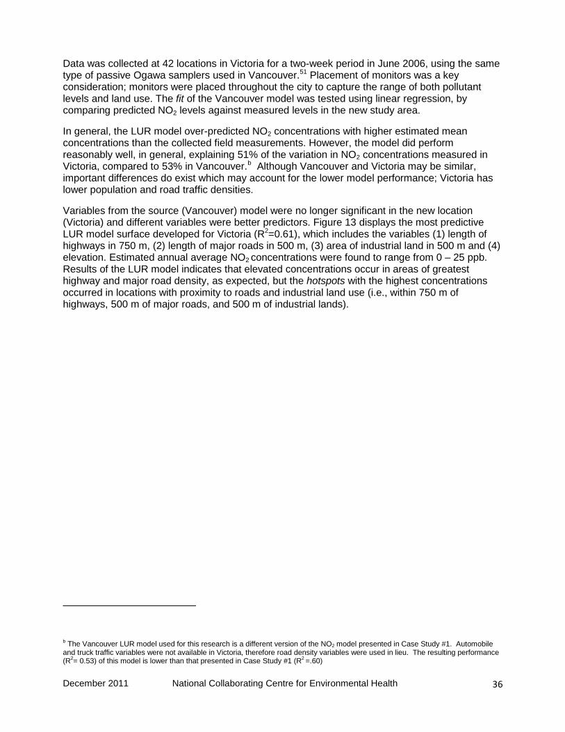
December 2011 National Collaborating Centre for Environmental Health 36
Data was collected at 42 locations in Victoria for a two-week period in June 2006, using the same type of passive Ogawa samplers used in Vancouver.51 Placement of monitors was a key consideration; monitors were placed throughout the city to capture the range of both pollutant levels and land use. The fit of the Vancouver model was tested using linear regression, by comparing predicted NO2 levels against measured levels in the new study area.
In general, the LUR model over-predicted NO2 concentrations with higher estimated mean concentrations than the collected field measurements. However, the model did perform reasonably well, in general, explaining 51% of the variation in NO2 concentrations measured in Victoria, compared to 53% in Vancouver.b
Variables from the source (Vancouver) model were no longer significant in the new location (Victoria) and different variables were better predictors. Figure 13 displays the most predictive LUR model surface developed for Victoria (R2=0.61), which includes the variables (1) length of highways in 750 m, (2) length of major roads in 500 m, (3) area of industrial land in 500 m and (4) elevation. Estimated annual average NO2 concentrations were found to range from 0 – 25 ppb. Results of the LUR model indicates that elevated concentrations occur in areas of greatest highway and major road density, as expected, but the hotspots with the highest concentrations occurred in locations with proximity to roads and industrial land use (i.e., within 750 m of highways, 500 m of major roads, and 500 m of industrial lands).
Although Vancouver and Victoria may be similar, important differences do exist which may account for the lower model performance; Victoria has lower population and road traffic densities.
b The Vancouver LUR model used for this research is a different version of the NO2 model presented in Case Study #1. Automobile and truck traffic variables were not available in Victoria, therefore road density variables were used in lieu. The resulting performance (R2= 0.53) of this model is lower than that presented in Case Study #1 (R2 =.60)
December 2011 National Collaborating Centre for Environmental Health 37
Figure 13 Land use regression map for NO2 in Victoria, based on field sampling in 200652
The results of this study are important for two reasons. Firstly, this work suggests that LUR models may transfer reasonably well to geographically similar areas. The ability to transfer a LUR model from a source region to other locations is very advantageous; such transfers may significantly reduce the time and expense necessary for conducting field monitoring campaigns and constructing new models. Secondly, the generation of distribution maps, based on results of the LUR in Victoria, allowed for a better understanding of NO2 distribution in the city. In contrast to a mean concentration level calculated at one site and applied to the entire region, the LUR surface captures the spatial variability and relative differences in concentrations at many sites throughout the region. Specifically, the LUR model developed for Victoria provided regulators with more detailed information on the variability of NO2 concentrations throughout the region than that captured by the fixed monitoring network, including areas of high and low concentrations.
December 2011 National Collaborating Centre for Environmental Health 38
Health Impact Assessment: A Direct Application
Introduction
Health impact assessments (HIA) describe the health impacts of a proposed or existing project, policy or program on a specific population. These assessments use a combination of procedures and methods to provide information on health implications and may take into account socio-economic as well as psychosocial effects. It serves as a valuable tool to address the impacts of air quality on health; examples of an HIA with an air quality focus include investigation of: health impacts of current air quality in a community; proposed industrial project that will contribute to local emissions; an evaluation of existing or proposed intervention targeted at reducing community exposures. Decision-makers can use HIA to determine if changes need to be made to a project, policy or program to minimize these health impacts. Conducting an HIA
There is no standard method to conduct an HIA. Assessments can vary in their complexity, ranging from an in-depth assessment, using formal steps to provide a comprehensive view of health, to a simpler risk assessment that investigates a specific health outcome. Generally, any HIA will include many of the following steps53:
• Initial screening: to identify a project, policy, or program for which a HIA is needed; • Scoping of potential health effects: to identify potential health effects to a population,
resulting from the project, program or policy; • Assessing risks and benefits: to identify any vulnerable/highly-exposed groups, as well as
to identify key stakeholders that may need to be consulted; • Developing recommendations: to suggest changes or alternatives that can lead to
prevention or reduction of health impacts; • Reporting of findings: to present HIA results to stakeholders and decision-makers; • Evaluation: to determine the impact of the HIA on the decisions relating to the program,
project or policy.
Several sources of information are used to conduct an HIA. For an assessment of air quality- related health impacts, the following may be used: information on source emissions, ambient concentrations, and community demographics, including information on vulnerable groups such as children and the elderly. Health-related information may include the incidence of specific health outcomes such as cancer or asthma rates, as well as other indicators, such as emergency room and physician visits. Additionally, epidemiological data conducted either locally or in other study locations can be used to provide information on the relationships between expected or background levels of pollutants and incidences of specific health outcomes, to assess local health impacts.
In Canada, all environmental impact assessments must incorporate an HIA component. An environmental impact assessment (EIA) is typically conducted before the initiation of a project, in order to determine its effects on the human and biophysical environment.54 The recognition that health was often overlooked in EIA and that health assessments were often limited or incomprehensive,55 led to the development of the Canadian Handbook of Health Impact
December 2011 National Collaborating Centre for Environmental Health 39
Assessment.54 According to the handbook, the purposes for incorporating HIA in the EIA method include the following:
• To address public concern; • To minimize the need for separate health and environmental assessment; • To ensure cost effectiveness; • To minimize the adverse and maximize the beneficial effects on health; • To support the concept of sustainable development.
The process of conducting an HIA generally involves several players, including the proponent of the project/program, government departments, ministries or agencies, health professionals, decision-makers, and the public. Strengths and Limitations HIA is an important tool which directly assesses the health impacts of a particular project, policy, or program. These assessments can be invaluable in limiting the health impacts related to local air quality because they provides concrete recommendations that are linked with expected health-related benefits. Often, HIA is not conduced, due to their time intensive nature. The assessment process however, can be flexible depending on the needs of the project; the HIA can evaluate a specific health outcome versus attempting to understand a larger view of health, as long as the objectives of such an assessment are made clear. More in-depth HIAs often fail to take into account the necessary data to conduct a comprehensive health assessment, particularly the social impacts that impact health. When conducting an HIA, common challenges include limited availability of data on the potential health effects of exposures, incomplete identification and evaluation of all the possible risks and benefits of a project/policy/program, and a failure to include all stakeholders.
Example 1 Air Quality Assessment Tools Guide – Example: Health Impact Assessment
Metro Vancouver Air Toxics Emission Inventory and Health Risk Assessment
Emissions of air toxics, also referred to as hazardous air pollutants, are primarily generated through human activities and are known or suspected to cause harmful effects on human health or the environment. Depending on the level of exposure, these health effects can be significant. To investigate health impacts of air toxics exposures in the Lower Fraser Valley (LFV), Metro Vancouver in partnership with Environment Canada commissioned a consultant study to:
• Develop an emissions inventory and a forecast of emissions of air toxics for the LFV; includes the Metro Vancouver region, the southwestern portion of the Fraser Valley Regional District, and Whatcom County in the State of Washington;
• Conduct a preliminary evaluation of the risk to human health from air toxics emissions in the LFV.
Air Toxics Emission Inventory
The inventory included emissions of air toxics from point sources (e.g., large industrial facilities), area sources (e.g., lighter industrial, commercial, institutional, residential, agricultural, and
December 2011 National Collaborating Centre for Environmental Health 40
naturally-occurring sources), and mobile sources (e.g., motor vehicles, non-road engines and equipment, aircraft, locomotives, and marine vessels). The list of inventoried air toxics included substances declared as toxic under the Canadian Environmental Protection Act and the United States Environmental Protection Agency’s (U.S. EPA) list of hazardous air pollutants. Emissions were quantified for 158 air toxics, such as formaldehyde, benzene, and diesel particulate matter. The resulting emission estimates were described by substance, emission source, year and location.
Health Risk Assessment
Based on the list of air toxics in the emission inventory, a subset of 39 prioritized air toxics was identified for inclusion in the health risk assessment (Table 3), using the following criteria:
• Precedence in the literature – Substance identified as a priority in other health risk assessments;
• Availability of health risk information from recognized sources – In general this meant that concentration response factors existed to relate the exposure concentrations of substances to human health impacts. These response factors include both unit risk factors, which estimate the additional risk of developing cancer, and reference exposure levels, which have been established through animal or epidemiological studies and reflect concentrations below which adverse health effects are not anticipated to occur.
• Availability of data to estimate the concentrations – Measurements available from the regional air quality monitoring network or predictions of the average concentration of air toxics to which the public would be exposed on a long-term basis in the LFV.
To characterize the risk associated with the prioritized air toxics, a screening analysis was performed to estimate 70-year lifetime cancer risk, expressed in cancer incidences per million population and a hazard quotient, where a quotient below 1.0 is not anticipated to result in adverse (non-cancer) health effects.
The 70-year lifetime cancer risk was calculated by multiplying the Unit Risk (UR), which is the additional risk of developing cancer given a 1 μg/m3 increase in the ambient concentration over a 70-year lifetime, by the estimated exposure concentration, as shown in the following equation:
Risk (per million) = UR (µg/m3)-1 x Estimated Exposure (µg/m3) x 106
The hazard quotient is estimated as the ratio of the estimated exposure concentration to the reference exposure level (REL), which is typically extrapolated from animal or epidemiological studies and incorporates a margin of safety designed to protect susceptible members of the population. Hazard quotients below 1 represent a level of exposure that is not anticipated to result in adverse health effects. Hazard quotients greater than 1 should not be interpreted as inherently dangerous, but present a level that exceeds the margin of safety for human exposure. A higher hazard quotient indicates a greater likelihood of observable health effects. The following illustrates the equation:
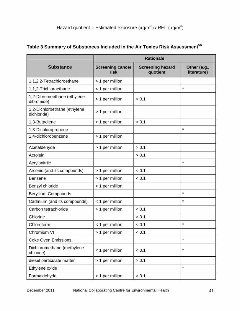
December 2011 National Collaborating Centre for Environmental Health 41
Hazard quotient = Estimated exposure (µg/m3) / REL (µg/m3)
Table 3 Summary of Substances Included in the Air Toxics Risk Assessment56
Substance
Rationale
Screening cancer risk
Screening hazard quotient
Other (e.g., literature)
1,1,2,2-Tetrachloroethane > 1 per million
1,1,2-Trichloroethane < 1 per million *
1,2-Dibromoethane (ethylene dibromide) > 1 per million > 0.1
1,2-Dichloroethane (ethylene dichloride) > 1 per million
1,3-Butadiene > 1 per million > 0.1
1,3-Dichloropropene * 1,4-dichlorobenzene > 1 per million
Acetaldehyde > 1 per million > 0.1
Acrolein > 0.1
Acrylonitrile *
Arsenic (and its compounds) > 1 per million < 0.1
Benzene > 1 per million < 0.1
Benzyl chloride > 1 per million
Beryllium Compounds *
Cadmium (and its compounds) < 1 per million *
Carbon tetrachloride > 1 per million < 0.1
Chlorine > 0.1
Chloroform < 1 per million < 0.1 *
Chromium VI > 1 per million < 0.1
Coke Oven Emissions *
Dichloromethane (methylene chloride) < 1 per million < 0.1 *
diesel particulate matter > 1 per million > 0.1
Ethylene oxide *
Formaldehyde > 1 per million > 0.1
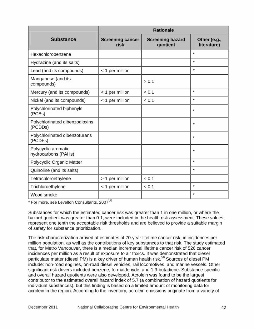
December 2011 National Collaborating Centre for Environmental Health 42
Substance
Rationale
Screening cancer risk
Screening hazard quotient
Other (e.g., literature)
Hexachlorobenzene *
Hydrazine (and its salts) *
Lead (and its compounds) < 1 per million *
Manganese (and its compounds) > 0.1
Mercury (and its compounds) < 1 per million < 0.1 *
Nickel (and its compounds) < 1 per million < 0.1 *
Polychlorinated biphenyls (PCBs) *
Polychlorinated dibenzodioxins (PCDDs) *
Polychlorinated dibenzofurans (PCDFs) *
Polycyclic aromatic hydrocarbons (PAHs) *
Polycyclic Organic Matter *
Quinoline (and its salts) *
Tetrachloroethylene > 1 per million < 0.1
Trichloroethylene < 1 per million < 0.1 *
Wood smoke * * For more, see Levelton Consultants, 200756
Substances for which the estimated cancer risk was greater than 1 in one million, or where the hazard quotient was greater than 0.1, were included in the health risk assessment. These values represent one tenth the acceptable risk thresholds and are believed to provide a suitable margin of safety for substance prioritization.
The risk characterization arrived at estimates of 70-year lifetime cancer risk, in incidences per million population, as well as the contributions of key substances to that risk. The study estimated that, for Metro Vancouver, there is a median incremental lifetime cancer risk of 526 cancer incidences per million as a result of exposure to air toxics. It was demonstrated that diesel particulate matter (diesel PM) is a key driver of human health risk.56 Sources of diesel PM include: non-road engines, on-road diesel vehicles, rail locomotives, and marine vessels. Other significant risk drivers included benzene, formaldehyde, and 1,3-butadiene. Substance-specific and overall hazard quotients were also developed. Acrolein was found to be the largest contributor to the estimated overall hazard index of 5.7 (a combination of hazard quotients for individual substances), but this finding is based on a limited amount of monitoring data for acrolein in the region. According to the inventory, acrolein emissions originate from a variety of
December 2011 National Collaborating Centre for Environmental Health 43
sources, including non-road sources (commercial jets and recreational marine vessels), gasoline-fueled motor vehicles, and other industrial sources.
The consultant study also compared the results to other similar studies for consistency, analyzed assumptions, and uncertainties associated with the work and provided recommendations for improving future assessments. While direct comparison of risk estimates with other published values is difficult, since there can be substantial variation in methodology, substances included, and exposure pathways considered between studies, a similar study conducted for the Puget Sound area estimated cancer risk from 447 to 622 per million population and a hazard index of 6.2. Other studies conducted for Portland, Oregon, the South Coast air basin (California), Minnesota, and Queen’s, New York were reviewed; with cancer risk ranging from 27 to as high as 1470 per million, and hazard indices from less than 1 to nearly 60. Again, the methods used in these studies differ considerably.
Policy Use
Partly due to the findings of the above study, Metro Vancouver established a Diesel Emission Reduction Program in 2009. The program recognized that reducing diesel emissions is an important step in improving air quality and public health in Metro Vancouver. As part of the program, given the contribution of non-road diesel engines to overall diesel emissions, exposure and health risk in the region, Metro Vancouver developed and adopted (in 2011) a bylaw to reduce emissions from older, in-use non-road diesel engines.57 The Province of BC also implemented requirements for diesel retrofits on older heavy-duty diesel trucks, recognizing the risk to health from diesel engine emissions.58 Several other governments are also taking actions to reduce emissions from diesel engines.
Conclusion
Specific tools exist to address different components of air quality, including sources, emissions, and topographical and meteorological conditions. Information generated from these tools can provide valuable information to help support the work of public health practitioners and decision-makers working to improve local air quality and limit the health impacts of air pollution.
References
1. Environment Canada. Pollutants. Gatineau, QC: Environment Canada; 2011 [cited 2011 Mar 11]; Available from: http://www.ec.gc.ca/Air/default.asp?lang=En&n=BCC0B44A-1. 2. British Columbia Ministry of Healthy Living and Sport. 2005 British Columbia emissions inventory of criteria air contaminants. Victoria, BC: Government of BC; 2009 Jul. Available from: http://www.bcairquality.ca/reports/pdfs/2005_emissions_inventory.pdf. 3. Metro Vancouver. 2005 Lower Fraser Valley air emissions inventory & forecast and backcast. Burnaby, BC: Metro Vancouver Policy & Planning Department, Air Quality Policy & Management Division; 2007 Dec. Available from: http://www.metrovancouver.org/about/publications/Publications/2005_LFV_Emissions.pdf. 4. Larson T, Su J, Baribeau AM, Buzzelli M, Setton E, Brauer M. A spatial model of urban winter woodsmoke concentrations. Environ Sci Technol. 2007 Apr 1;41(7):2429-36. 5. Künzli N, Avol E, Wu J, Gauderman WJ, Rappaport E, Millstein J, et al. Health effects of the 2003 Southern California wildfires on children. Am J Respir Crit Care Med. 2006;174(11):1221-8.
December 2011 National Collaborating Centre for Environmental Health 44
6. Delfino RJ, Brummel S, Wu J, Stern H, Ostro B, Lipsett M, et al. The relationship of respiratory and cardiovascular hospital admissions to the southern California wildfires of 2003. Occup Environ Med. 2009;66(3):189-97. 7. Health Effects Institute. Traffic-related air pollution: A critical review of the literature on emissions, exposure, and health effects. Boston, MA: HEI; 2009. Available from: http://pubs.healtheffects.org/view.php?id=334. 8. Pope C, Dockery D. Health effects of fine particulate air pollution: Lines that connect. J Air Waste Manage. 2006;56(6):709-42. 9. Brook RD, Franklin B, Cascio W, Hong Y, Howard G, Lipsett M, et al. Air pollution and cardiovascular disease: A statement for healthcare professionals from the Expert Panel on Population and Prevention Science of the American Heart Association. Circulation. 2004 Jun;109(21):2655-71. 10. Chen TM, Gokhale J, Shofer S, Kuschner WG. Outdoor air pollution: Ozone health effects. Am J Med Sci. 2007 Apr;333(4):244-8. 11. Hesterberg TW, Bunn WB, McClellan RO, Hamade AK, Long CM, Valberg PA. Critical review of the human data on short-term nitrogen dioxide (NO2) exposures: Evidence for NO2 no-effect levels. Crit Rev Toxicol. 2009;39(9):743-81. 12. Duclos P, Sanderson LM, Lipsett M. The 1987 forest fire disaster in California - assessment of emergency room visits. Arch Environ Health. 1990;45(1):53-8. 13. Moore D, Copes R, Fisk R, Joy R, Chan K, Brauer M. Population health effects of air quality changes due to forest fires in British Columbia in 2003: Estimates from physician-visit billing data. Can J Public Health. 2006;97(2):105-8. 14. Border Air Quality Study. Summary findings from the Border Air Quality Study. Vancouver, BC: Health Canada and the BC Centre for Disease Control; 2008 Mar. Available from: http://www.cher.ubc.ca/UBCBAQS/Reports/BAQS_Summary_Mar08.pdf. 15. British Columbia Ministry of Environment. Environmental best management practices for urban and rural land development in British Columbia: Air quality BMPs and supporting information. Victoria, BC: Government of BC; 2006 Feb. Available from: http://www.bcairquality.ca/reports/pdfs/aqbmps_feb16_06.pdf. 16. British Columbia Ministry of the Environment. Air quality monitoring. Victoria, BC: Government of BC; 2010 [cited 2010 Jul 22]; Available from: http://www.bcairquality.ca/assessment/air-quality-monitoring.html. 17. British Columbia Ministry of the Environment. Network description. Victoria, BC: Government of BC; 2010 [cited 2010 Jul 21]; Available from: http://www.env.gov.bc.ca/epd/bcairquality/assessment/network-description.html. 18. Huang L, cartographer. BCMOE central monitoring station locations. Victoria, BC: British Columbia Ministry of the Environment; 2011. 19. Metro Vancouver. Lower Fraser Valley Ambient Air Quality Report – 2009. Burnaby, BC: Metro Vancouver, Policy & Planning Department, Air Quality Policy & Management Division; 2010 Dec. Available from: http://www.metrovancouver.org/about/publications/Publications/2009_LFV_Air_Quality_Report-final.pdf. 20. Sonoma Technology. Framework for the British Columbia Air Monitoring Network. Final report STI-906059.05-3229-FR. Victoria, BC: Prepared for British Columbia Ministry of the Environment; 2008 Jun. Available from: http://www.env.gov.bc.ca/epd/bcairquality/reports/pdfs/framework_bc_air_mon_net.pdf. 21. British Columbia Ministry of the Environment. BC Air Quality. The Mobile Air Monitoring Laboratory (MAML). Victoria, BC: Government of British Columbia; 2010 [cited 2010 Oct 20]; Available from: http://www.env.gov.bc.ca/epd/bcairquality/readings/maml.html. 22. Photo courtesy of Mark Graham. Mobile Air Monitoring Laboratory (MAML) operated by BC Ministry of Environment. Victoria, BC: British Columbia Ministry of the Environment; 2011.
December 2011 National Collaborating Centre for Environmental Health 45
23. Government of British Columbia. RSBC 1996, Local Government Act. RSBC 1996. (2010). Available from: http://www.bclaws.ca/EPLibraries/bclaws_new/document/ID/freeside/96323_00. 24. Nowlan L, Rolfe C, GrantI K. The Smart Growth guide to local government law and advocacy. Vancouver, BC: West Coast Environmental Law Research Foundation; 2001. Available from: http://wcel.org/sites/default/files/publications/The%20Smart%20Growth%20Guide%20to%20Local%20Government%20Law%20and%20Advocacy.pdf. 25. Alderson J. Inventory of air quality bylaws in British Columbia for: Anti-idling, open burning, and wood-burning appliances. Victoria, BC: British Columbia Ministry of the Environment; 2007. Available from: http://www.bcairquality.ca/reports/pdfs/aq_bylaws_bc.pdf. 26. British Columbia Ministry of the Environment. Develop with care: Environmental guidelines for urban and rural land development in British Columbia. Victoria, BC: Government of BC; 2006 Mar. Available from: http://www.env.gov.bc.ca/wld/documents/bmp/devwithcare2006/develop_with_care_intro.html. 27. Stieb DM, Burnett RT, Smith-Doiron M, Brion O, Shin HH, Economou V. A new multipollutant, no-threshold air quality health index based on short-term associations observed in daily time-series analyses. J Air Waste Manag Assoc. 2008 Mar;58(3):435-50. 28. U.S. Environmental Protection Agency. Emissions factors & AP 42, Compilation of aIr pollutant emissions factors. Washington, DC: EPA; 2010 [cited 2010 October 13]; Available from: http://www.epa.gov/ttnchie1/ap42/. 29. Environment Canada. National pollutant release inventory. Gatineau, QC: Government of Canada; 2010 [cited 2010 Oct 18]; Available from: http://www.ec.gc.ca/inrp-npri/default.asp?lang=En&n=4A577BB9-1. 30. Government of Canada. Canada Gazette. Ottawa, ON. 2010 [cited 2010 Oct 13]; Available from: http://www.gazette.gc.ca/index-eng.html. 31. Krzyzanowski J. The importance of policy in emissions inventory accuracy--a lesson from British Columbia, Canada. J Air Waste Manag Assoc. 2009 Apr;59(4):430-9. 32. AirCare. The vehicle emissions testing program for Vancouver and the Fraser Valley. Burnaby, BC: Pacific Vehicle Testing Technologies Ltd; 2010 [cited 2010 Dec 2]; Available from: http://www.aircare.ca/. 33. British Columbia Ministry of Environment. Guidelines for air quality dispersion modelling in British Columbia. Victoria, BC: Government of BC; 2008. Available from: http://www.bcairquality.ca/reports/pdfs/air_disp_model_08.pdf. 34. British Columbia Ministry of the Environment. A primer on the guidelines for air quality dispersion modelling in British Columbia. Victoria, BC: Government of BC; 2006 Oct. Available from: http://www.env.gov.bc.ca/epd/bcairquality/reports/pdfs/aq_disp_model_06_primer.pdf. 35. Stantec. Prince George Air Quality Dispersion Modelling Study – a revision. Final report. Project No.:1231-10153. Prince George, BC: Prepared for Ministry of Environment , Environmental Protection Division and Prince George Air Improvement Roundtable; 2010 Oct. Available from: http://pgairquality.com/uploads/files/pdf/123110153%20Final%20PG%20AIR_MOE_08-Oct-2010.pdf. 36. Meyen S. Presentation to the annual general meeting of the Bulkley Valley Lakes District Airshed Managment Society. Smithers, BC; 2005. 37. Millar G, Abel T, Allen J, Barn P, Noullett M, Spagnol J, et al. Evaluating human exposure to fine particulate matter part II: Modeling. Geography Compass. 2010;4(7):731-49. 38. Evans GJ, Jeong C-H. Data analysis and source apportionment of PM2.5 in Golden, British Columbia using Positive Matrix Factorization (PMF). Toronto, ON: University of Toronto; 2007 Apr Contract No.: Environment Canada K 2313-06-0015. SOCAAR Report No.: CR-WB-2007-02. Available from: http://www.env.gov.bc.ca/epd/regions/kootenay/aq_reports/golden_pmf/golden_pmf.pdf.
December 2011 National Collaborating Centre for Environmental Health 46
39. Rubin JI, Brow SG, Hafner HR, Roberts PT, (Sonoma Technology Inc). Source apportionment of PM2.5 in Prince George, British Columbia. Final report: Prepared for British Columbia Ministry of the Environment; 2008 Feb; Contract No.: STI-906052.06-3268-FR. 40. Isakov V, Touma JS, Khlystov A. A method of assessing air toxics concentrations in urban areas using mobile platform measurements. J Air Waste Manag Assoc. 2007 Nov;57(11):1286-95. 41. Jeong C-H, Hopke PK, Kim E, Lee D-W. The comparison between thermal-optical transmittance elemental carbon and Aethalometer black carbon measured at multiple monitoring sites. Atmos Environ. 2004;38(31):5193-204. 42. Millar G. Air quality monitoring data, Terrace. From the WEST (Wood Stove Exchange STudy). Available from: http://www.cher.ubc.ca/woodstove/welcome.htm. 43. Ruzer LS, Harley NH, editors. Aerosols handbook measurement, dosimetry, and health effects. Boca Raton, FL: CRC Press; 2005. Available from: http://dx.doi.org/10.1201/9780203493182. 44. Poplawski K, Setton E, (University of Victoria Spatial Sciences Research Laboratory). MAML - Mobile Air Monitoring Laboratory. Collection report - James Bay Air Quality Study, June -August 2009. Victoria, BC: Prepared for Vancouver Island Health Authority, BC Ministry of the Environment; 2010 Jan. Available from: http://www.viha.ca/NR/rdonlyres/E9167F08-04E0-4A72-A303-F2B0BD1054B7/0/jbaq_maml_2010.pdf. 45. Dockery D, Pope C, Xu X, Spengler J, Ware J, Fay M, et al. An association between air pollution and mortality in six U.S. cities. N Engl J Med. 1993;329:1753-9. 46. Hoek G, Beelen R, de Hoogh K, Vienneau D, Gulliver J, Fischer P, et al. A review of land-use regression models to assess spatial variation of outdoor air pollution. Atmos Environ. 2008;42(33):7561-78. 47. Gilbert NL, Goldberg MS, Beckerman B, Brook JR, Jerrett M. Assessing spatial variability of ambient nitrogen dioxide in Montreal, Canada, with a land-use regression model. J Air Waste Manag Assoc. 2005 Aug;55(8):1059-63. 48. Jerrett M, Arain MA, Kanaroglou P, Beckerman B, Crouse DL, Gilbert NL, et al. Strategies for clean air and health. In: Craig L, Krewski D, Shortreed J, Samet J, editors. AIRNET Annual Conference/ NERAM International Colloquium, Nov 5 – 7, 2003; Rome, Italy: Institute of Risk Research; 2005 Jul. p. 19-34. Available from: http://www.irr-neram.ca/CQ3Rome/Proceedings/Entire_Document.pdf#page=27. 49. Henderson SB, Beckerman B, Jerrett M, Brauer M. Application of land use regression to estimate long-term concentrations of traffic-related nitrogen oxides and fine particulate matter. Environ Sci Technol. 2007 Apr;41(7):2422-8. 50. Henderson S. Land use regression map for NO in greater Vancouver based on results of the 2003 study. 2007. 51. Poplawski K, Gould T, Setton E, Allen R, Su J, Larson T, et al. Intercity transferability of land use regression models for estimating ambient concentrations of nitrogen dioxide. J Expo Sci Environ Epidemiol. 2009 Jan;19(1):107-17. 52. Poplawski K. Land use regression map for NO2 in Victoria, based on field sampling in 2006. Victoria, BC: University of Victoria, Spatial Sciences Research Laboratory, Department of Geography. 53. Centers for Disease Control and Prevention. Health impact assessment. Atlanta, GA: CDC; 2010 [cited 2010 Jul 30 ]; Available from: http://www.cdc.gov/healthyplaces/hia.htm. 54. Health Canada. Canadian handbook on health impact assessment. Volume 1. The basics. Ottawa, ON: Ministry of Health; 2004 Nov. Available from: http://publications.gc.ca/collections/Collection/H46-2-04-363E.pdf.
December 2011 National Collaborating Centre for Environmental Health 47
55. Davies K, Sadler B. Environmental assessment and human health: Perspectives, approaches, and future directions. A background report for the International Study of the Effectiveness of Environmental Assessment. Ottawa, ON: Health Canada; 1997 May. Available from: http://www.hc-sc.gc.ca/ewh-semt/alt_formats/hecs-sesc/pdf/pubs/eval/health-perspective-sante/human_health-sante_humaine-eng.pdf. 56. Levelton Consultants Ltd. Air toxics emissions inventory and health risk assessment - Summary report. Burnaby, BC: Prepared for Greater Vancouver Regional District and Environment Canada; 2007 Nov. Available from: www.metrovancouver.org/about/publications/Publications/Air_Toxics_Emission.pdf. 57. Metro Vancouver. Non-Road Diesel Engine Emission Regulation Bylaw No. 1137, 2011. Metro Vancouver Policy & Planning Department, Air Quality Policy & Management Division (2011). Available from: www.metrovancouver.org/services/permits/DieselEmissions. 58. British Columbia Ministry of Transportation and Infrastructure. Commercial vehicle safety and enforcement: Diesel retrofit. Victoria, BC: Government of BC; 2011 [cited 2011 May 2]; Available from: http://www.th.gov.bc.ca/cvse/diesel_retrofit/.
This document was produced by the National Collaborating Centre for Environmental Health in December 2011.
Permission is granted to reproduce this document in whole, but not in part.
Production of this document has been made possible through a financial contribution from the Public Health Agency of Canada.
ISBN: 978-1-926933-37-5
© National Collaborating Centre for Environmental Health 2011
400 East Tower 555 W 12th Avenue Vancouver, BC V5Z 3X7 Tel.: 604-707-2445 Fax: 604-707-2444 [email protected]
www.ncceh.ca
To provide feedback on this document, please visit www.ncceh.ca/en/document_feedback