Atmos. Chem. Phys., 20, 14597–14616, 2020https://doi.org/10.5194/acp-20-14597-2020© Author(s) 2020. This work is distributed underthe Creative Commons Attribution 4.0 License.

Air quality impact of the Northern California Camp Fire ofNovember 2018Brigitte Rooney1, Yuan Wang1,2, Jonathan H. Jiang2, Bin Zhao3, Zhao-Cheng Zeng4, and John H. Seinfeld5

1Division of Geological and Planetary Sciences, California Institute of Technology, Pasadena, CA, USA2Jet Propulsion Laboratory, California Institute of Technology, Pasadena, CA, USA3Pacific Northwest National Laboratory, Richland, WA, USA4Joint Institute for Regional Earth System Science and Engineering, University of California, Los Angeles, CA, USA5Division of Chemistry and Chemical Engineering, California Institute of Technology, Pasadena, CA, USA

Correspondence: Yuan Wang (yuan.wang@caltech.edu) and John H. Seinfeld (seinfeld@caltech.edu)

Received: 3 June 2020 – Discussion started: 8 July 2020Revised: 20 September 2020 – Accepted: 30 September 2020 – Published: 1 December 2020

Abstract. The Northern California Camp Fire that took placein November 2018 was one of the most damaging environ-mental events in California history. Here, we analyze ground-based station observations of airborne particulate matter thathas a diameter < 2.5 µm (PM2.5) across Northern Califor-nia and conduct numerical simulations of the Camp Fire us-ing the Weather Research and Forecasting model online cou-pled with chemistry (WRF-Chem). Simulations are evaluatedagainst ground-based observations of PM2.5, black carbon,and meteorology, as well as satellite measurements, suchas Tropospheric Monitoring Instrument (TROPOMI) aerosollayer height and aerosol index. The Camp Fire led to anincrease in Bay Area PM2.5 to over 50 µgm−3 for nearly2 weeks, with localized peaks exceeding 300 µgm−3. Us-ing the Visible Infrared Imaging Radiometer Suite (VIIRS)high-resolution fire detection products, the simulations re-produce the magnitude and evolution of surface PM2.5 con-centrations, especially downwind of the wildfire. The over-all spatial patterns of simulated aerosol plumes and theirheights are comparable with the latest satellite products fromTROPOMI. WRF-Chem sensitivity simulations are carriedout to analyze uncertainties that arise from fire emissions,meteorological conditions, feedback of aerosol radiative ef-fects on meteorology, and various physical parameteriza-tions, including the planetary boundary layer model and theplume rise model. Downwind PM2.5 concentrations are sen-sitive to both flaming and smoldering emissions over the fire,so the uncertainty in the satellite-derived fire emission prod-ucts can directly affect the air pollution simulations down-

wind. Our analysis also shows the importance of land surfaceand boundary layer parameterization in the fire simulation,which can result in large variations in magnitude and trend ofsurface PM2.5. Inclusion of aerosol radiative feedback mod-erately improves PM2.5 simulations, especially over the mostpolluted days. Results of this study can assist in the develop-ment of data assimilation systems as well as air quality fore-casting of health exposures and economic impact studies.

1 Introduction

Wildfires have become increasingly prevalent in Califor-nia. It has been reported that, between 2007 and 2016,as many as 3672 fires occurred in California, consumingup to 1759 km−2 (Pimlott et al., 2016). Increasingly, thepopulation has expanded into high-fire-risk areas and nearwildland–urban interfaces (Brown et al., 2020). The intensesmoke consisting of airborne particulate matter of diame-ter < 2.5 µm (PM2.5) associated with these fires leads to anincreased risk of morbidity and mortality (Cascio, 2018).PM2.5 from wildfires consists of a spectrum of light scatter-ing and absorptive particles largely comprising organic andblack carbon. It is increasingly important to understand thecause and nature of wildfires as the number of extreme eventsand the length of the wildfire season continue to grow (Kahn,2020; Shi et al., 2019). Fire-related studies have estimatedexposures to PM2.5 based on ground-level monitoring-stationmeasurements (Shi et al., 2019; Herron-Thorpe et al., 2014;

Published by Copernicus Publications on behalf of the European Geosciences Union.

14598 B. Rooney et al.: Air quality impact of the Northern California Camp Fire of November 2018

Archer-Nicholls et al., 2015). Spatial coverage of such mon-itoring stations often tends to be scarce, especially in ruralareas. Satellite remote sensing offers a powerful method tomonitor air quality during fire events. One study used ra-diance measurements from the Tropospheric Monitoring In-strument (TROPOMI) to derive atmospheric carbon monox-ide and assess the resulting air quality burden in major citiesdue to emissions from the California wildfires from Novem-ber 2018 (Schneising et al., 2020). Ideally, analysis of fireevents is based on a combination of satellite-based mea-surements and ground-level observations to obtain spatialand temporal distributions of emissions. The Camp Fire ofNovember 2018 was, to date, the deadliest and most de-structive wildfire in California (Kahn, 2020; Brown et al.,2020). Originating along the Sierra Nevada mountain range,smoke from the fire spread across the Sacramento Valley tothe San Francisco Bay Area. Peak levels of PM2.5 in the SanFrancisco area exceeded 200 µgm−3 and remained above50 µgm−3 for nearly 2 weeks.

Numerous studies have addressed wildfire events usinga variety of model frameworks and data sources (Shi etal., 2019; Herron-Thorpe et al., 2014; Archer-Nicholls etal., 2015; Sessions et al., 2011). Shi et al. (2019) usedthe Weather Research and Forecasting model online cou-pled with chemistry (WRF-Chem) with Moderate ResolutionImaging Spectroradiometer (MODIS) and Visible InfraredImaging Radiometer Suite (VIIRS) fire data to study thewildfire of December 2017 in Southern California. Herron-Thorpe et al. (2014) evaluated simulations of the 2007 and2008 wildfires in the Pacific Northwest using the Commu-nity Multi-scale Air Quality (CMAQ) model with fire emis-sions generated by the BlueSky framework and fire locationsdetermined by the Satellite Mapping Automated ReanalysisTool for Fire Incident Reconciliation (SMART-FIRE). Thatstudy suggested that underprediction of PM2.5 was the re-sult of underestimated burned area as well as underpredictedsecondary organic aerosol (SOA) production and incom-plete speciation of SOA precursors within the CMAQ model.Archer-Nicholls et al. (2015) simulated biomass burningaerosol during the 2012 dry season in Brazil using WRF-Chem and fire emissions prepared from MODIS. That studyproposed that biases in the model were likely a result ofuncertainty in the plume injection height and emissions in-ventory, as well as simulated aerosol sinks (e.g., wet de-position), and lack of inclusion of SOA production in theModel for Simulating Aerosol Interactions and Chemistry(MOSAIC). Sessions et al. (2011) investigated methods forinjecting wildfire emissions using WRF-Chem. That studytested two fire data preprocessors: PREP-CHEM-SRC (in-cluded with WRF-Chem) and the Naval Research Labora-tory’s Fire Locating and Monitoring of Burning Emissions(FLAMBE), and three injection methods: the 1-D plume risemodel within WRF-Chem, releasing emissions only withinthe planetary boundary layer, and releasing emissions be-tween 3 and 5 km. That study compared results from sim-

ulating wildfires during the NASA Arctic Research of theComposition of the Troposphere from Aircraft and Satellites(ARCTAS) field campaign in 2008 with satellite data. Ses-sions et al. (2011) found that differences in injection heightsresult in different transport pathways.

The present study is a comprehensive investigation ofair quality impacts of the Camp Fire using a combinedanalysis of ground-based and space-borne observations andWRF-Chem simulations. Descriptions of the observation andmodel are presented in Sect. 2; model evaluation is presentedin Sect. 3; results of analysis are given in Sect. 4, followedby discussion and conclusion in Sect. 5.

2 Model description and observational data

The present study employs WRF-Chem (version 3.8.1)driven by the latest version of meteorological reanalysis datafor initialization and boundary conditions. Fire emissions aredetermined by pairing active fire location data from the VI-IRS satellite with the Brazilian Biomass Burning EmissionModel (3BEM), which calculates species mass emissionsfrom the burned biomass carbon density, combustion factors,emission factors, and the burning area. WRF-Chem simu-lations are evaluated against EPA surface observations andTROPOMI satellite products.

2.1 WRF-Chem configuration

The WRF-Chem simulation time period is 7 November 2018(a day before the fire began) to 22 November 2018 (when thefire was 90 % contained). We carried out simulations overtwo domains (Fig. 1): domain d01 includes all of Califor-nia at 8km× 8km horizontal resolution, while domain d02covers Northern California at 2km× 2km horizontal resolu-tion. A total of 49 vertical layers are used from the surface to100 hPa with 50 m vertical resolution in the planetary bound-ary layer. The meteorological boundary and initial conditionsfor the outer domain are generated from the fifth generationof European Centre for Medium-range Weather Forecasts(ECMWF) reanalysis dataset (ERA5) at 30km× 30km res-olution (Copernicus Climate Change Service, 2017). Chem-ical boundary and initial conditions for the outer domain aregenerated from the Model for Ozone and Related ChemicalTracers version 4 (MOZART-4).

We use physical options of the Noah Land-Surface Model(Tewari et al., 2004), the Mellor–Yamada–Janjic (MYJ)boundary layer scheme (Janjic, 1994), and the Rapid Radia-tive Transfer Model (RRTM) (longwave) and Dudhia (short-wave) radiative transfer schemes (Dudhia, 1989). Cumulusparameterization is not included. The second-generation Re-gional Acid Deposition Model (RADM2) chemical mech-anism coupled with the Modal Aerosol Dynamics modelfor Europe (MADE) and Secondary Organic Aerosol Model(SORGAM) (Zhao et al., 2011) are employed. Aerosol opti-

Atmos. Chem. Phys., 20, 14597–14616, 2020 https://doi.org/10.5194/acp-20-14597-2020

B. Rooney et al.: Air quality impact of the Northern California Camp Fire of November 2018 14599

Figure 1. Study domain (a) and observation station locations (b, c). Domain d01 covers the western US with a horizontal resolution of8 km. Domain d02 is centered over Northern California with a horizontal resolution of 2 km. AQS and NCDC observation sites are shown inpanels (b) and (c), where stations marked in green measure only PM2.5, stations in blue measure wind and temperature, stations in orangemeasure both PM2.5 and meteorology, and stations in yellow measure temperature only. Additionally, BC and CO are measured at 8 and 12sites in the Bay Area, respectively. © Google 2020.

cal properties are calculated based on the volume approxima-tion, for which the volume average of each aerosol species isused to calculate refractive indices (Jin et al., 2015). Aerosolradiative feedbacks on meteorology and chemistry are in-cluded in the simulations.

We use the National Emission Inventory for anthropogenicemissions (US EPA, 2018). Biogenic emissions are calcu-lated online using the Guenther scheme (Guenther et al.,2006). Dust emissions are calculated online using the God-dard Chemistry Aerosol Radiation and Transport (GOCART)dust emission scheme with University of Cologne (UOC)modifications (Shao et al., 2011). Sea salt emissions are ex-cluded. Technical details of wildfire emissions and the plumerise calculation are discussed in the next section.

2.2 Fire emissions inventory and plume rise model

Wildfire emissions are generated using the PREP-CHEM-SRC v1.5 preprocessor (Freitas et al., 2011) employing3BEM (Longo et al., 2010) with satellite data on detectedfires. For each pixel with fire detected, the mass of emittedspecies is calculated by

M [η]= αveg ·βveg ·EF[η]

veg · afire (1)

for a certain species η, where αveg is the carbon density(the mass of burnable aboveground biomass per unit areaof vegetation), βveg is the combustion factor, EFveg is theemission factor by species and vegetation type, and afire isthe burning area of each fire pixel. Vegetation type is gen-erated from the MODIS data following the InternationalGeosphere-Biosphere Programme (IGBP) land cover clas-sification. Vegetation-type-specific emission factors (EFveg)

and combustion factors (βveg) are derived from Ward etal. (1992) and Andreae and Merlet (2001). Vegetation-type-specific carbon density (αveg) is based on Olson et al. (2000)and Houghton et al. (2001). Active fire detection is retrievedfrom the VIIRS fire product with 375 m spatial resolution.A limitation of the VIIRS fire count product is its relativelylow temporal resolution. As a polar-orbiting satellite, VIIRSprovides fire detection during the daytime only once (about13:30 local time; LT) at each location.

The emission preprocessor generates a file formatted forWRF-Chem containing the smoldering-phase surface emis-sion fluxes of each species, the fire size for each vegeta-tion type, and flaming factor. Flaming factor is the ratio ofbiomass consumed in the flaming phase to biomass con-sumed in the smoldering phase. The 17 IGBP land coverclasses are aggregated into four main types: tropical forest,extratropical forest, savanna, and grassland. The size of thewildfire and phase of combustion play important roles in thestructure of the plume and the vertical distribution of emis-sions. Wildfire combustion is generally considered to occurin two phases: smoldering and flaming. Emissions from thesmoldering phase are allotted to the first layer of the compu-tational grid, while those from the flaming phase are releasedat injection heights above the surface, as determined by theplume rise model described below. Fire size determines thetotal surface heat flux, as well as the entrainment radius of theplume. Fire parameters are ascribed a daily temporal resolu-tion and are distributed to the WRF-Chem domains. The fireparameters are then input to the plume rise model (Freitas etal., 2007, 2010). The plume rise model is a one-dimensionalmodel implemented in each WRF-Chem grid cell with an in-dependent vertical grid resolution of 100 m. It calculates the

https://doi.org/10.5194/acp-20-14597-2020 Atmos. Chem. Phys., 20, 14597–14616, 2020

14600 B. Rooney et al.: Air quality impact of the Northern California Camp Fire of November 2018

Figure 2. Plume rise model schematic. For each grid cell in whichwildfire occurs, the plume rise model uses satellite fire products andthe surrounding WRF-Chem environmental conditions to calculatetwo plume-top heights by using the land-type-dependent minimumand maximum wildfire heat fluxes. Smoldering-phase emissions areallotted to the surface layer, while flaming-phase emissions are dis-tributed linearly aloft within the injection layers at a vertical resolu-tion of 100 m.

maximum height to which a plume reaches and distributesemissions therein (Fig. 2). The plume-top height, determinedby the surface heat flux from the fire and the thermody-namic stability of the atmospheric environment, is definedas the height at which the in-plume parcel vertical veloc-ity < 1 ms−1. The plume rise model uses upper and lowerbounds of heat fluxes determined by each land type to calcu-late the minimum and maximum plume-top height. Flamingemissions are distributed equally to each vertical level withinthe injection layer with the following calculation: flamingemissions per level are equal to the smoldering emission mul-tiplied by the flaming factor multiplied by DZ−1, where DZis the minimum plume-top height subtracted from the maxi-mum plume-top height. The model also accounts for entrain-ment, water balance, and internal gravity wave damping.

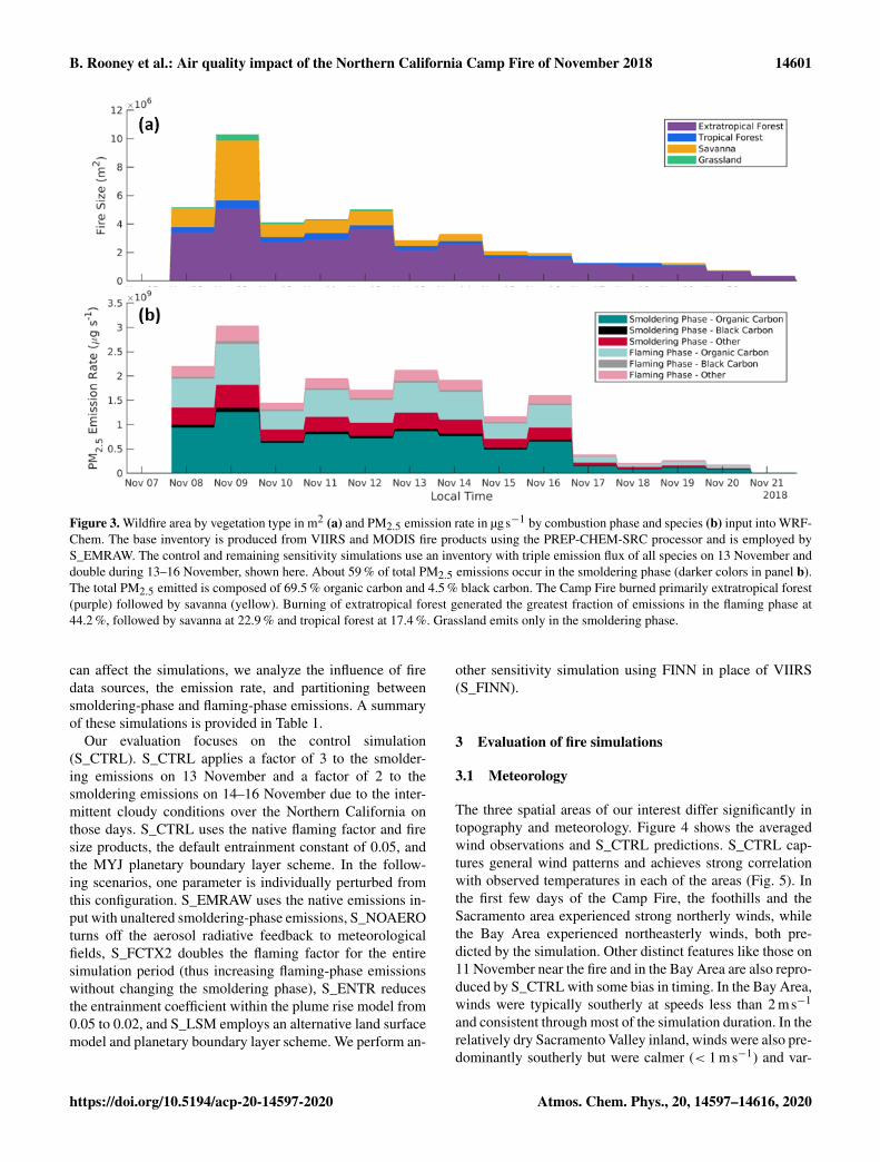
Figure 3 shows the fire size and particulate matter emis-sions produced from MODIS and VIIRS data. The Camp Fireburned primarily extratropical forest vegetation (which com-prised 68 % of the total burned area), followed by savanna(23 % of total area). The flaming emission rate for species n

from vegetation type v, is calculated by

flaming-phase raten,v =∑

fire cellsareav

· smoldering-phase fluxn·flaming factorv. (2)

At maximum, the carbon monoxide (CO) emission fluxwas 4.1× 107 molkm−2 h−1, and PM2.5 flux was 3.7×104 µgm−2 s−1. On average, 46 % of the fuel burned is es-timated to have been consumed during the flaming phase.

The Fire Inventory from NCAR (FINN) version 1.5(Wiedinmyer, 2011) is another fire emissions product thatwe will test in a sensitivity analysis. It is assembled for at-mospheric chemistry models with a daily temporal resolu-tion and a 1 km horizontal resolution. FINN is generatedusing satellite observations of active fires and land coverpaired with emission factors and fuel loading estimates. Theemissions are allocated to a diurnal cycle following WRAP(2005). FINN outputs the total wildfire emission flux, firesize, and land type fraction. As FINN does not include asmoldering- to flaming-phase ratio, the plume rise model cal-culates a ratio based on CO emissions.

2.3 Surface and satellite observations

The observational data include both ground-based measure-ments and satellite observations. Meteorological and surfaceconcentration data were obtained from the NOAA’s NationalClimatic Data Center (NCDC) and EPA Air Quality System(AQS), respectively. We focus on three areas: the region clos-est to the fire, the Sacramento Metro Area (population of2.5 million), and the San Francisco Bay Area (population of7 million). Hourly observations of wind speed at 10 m, winddirection at 10 m, temperature at 2 m, PM2.5, black carbon(BC), and CO are available for the sites shown in Fig. 1. Weuse level-2 products from the TROPOMI aboard the Coper-nicus Sentinel-5 Precursor (S5P) satellite to evaluate thespatial and vertical distribution of predictions. We compareTROPOMI aerosol layer height retrievals (3.5km× 7km)with the predicted WRF-Chem height of maximum PM2.5,and ultraviolet aerosol index (UVAI, 3.5km×7km) with thepredicted WRF-Chem BC columns. The model results aresampled around 13:30 LT when S5P passes over California.

2.4 Control and sensitivity simulations

To investigate the effects of key model parameters on theability to predict the atmospheric impact of the wildfire,we conduct a range of sensitivity simulations. As meteorol-ogy and atmospheric structure play important roles in plumedynamics and the transport of particulate matter, we sep-arately perturb the aerosol radiative feedback to meteorol-ogy, the planetary boundary layer parameterization, and theplume entrainment coefficient. To understand further the ex-tent to which fire characteristics provided by satellite data

Atmos. Chem. Phys., 20, 14597–14616, 2020 https://doi.org/10.5194/acp-20-14597-2020

B. Rooney et al.: Air quality impact of the Northern California Camp Fire of November 2018 14601

Figure 3. Wildfire area by vegetation type in m2 (a) and PM2.5 emission rate in µgs−1 by combustion phase and species (b) input into WRF-Chem. The base inventory is produced from VIIRS and MODIS fire products using the PREP-CHEM-SRC processor and is employed byS_EMRAW. The control and remaining sensitivity simulations use an inventory with triple emission flux of all species on 13 November anddouble during 13–16 November, shown here. About 59 % of total PM2.5 emissions occur in the smoldering phase (darker colors in panel b).The total PM2.5 emitted is composed of 69.5 % organic carbon and 4.5 % black carbon. The Camp Fire burned primarily extratropical forest(purple) followed by savanna (yellow). Burning of extratropical forest generated the greatest fraction of emissions in the flaming phase at44.2 %, followed by savanna at 22.9 % and tropical forest at 17.4 %. Grassland emits only in the smoldering phase.

can affect the simulations, we analyze the influence of firedata sources, the emission rate, and partitioning betweensmoldering-phase and flaming-phase emissions. A summaryof these simulations is provided in Table 1.

Our evaluation focuses on the control simulation(S_CTRL). S_CTRL applies a factor of 3 to the smolder-ing emissions on 13 November and a factor of 2 to thesmoldering emissions on 14–16 November due to the inter-mittent cloudy conditions over the Northern California onthose days. S_CTRL uses the native flaming factor and firesize products, the default entrainment constant of 0.05, andthe MYJ planetary boundary layer scheme. In the follow-ing scenarios, one parameter is individually perturbed fromthis configuration. S_EMRAW uses the native emissions in-put with unaltered smoldering-phase emissions, S_NOAEROturns off the aerosol radiative feedback to meteorologicalfields, S_FCTX2 doubles the flaming factor for the entiresimulation period (thus increasing flaming-phase emissionswithout changing the smoldering phase), S_ENTR reducesthe entrainment coefficient within the plume rise model from0.05 to 0.02, and S_LSM employs an alternative land surfacemodel and planetary boundary layer scheme. We perform an-

other sensitivity simulation using FINN in place of VIIRS(S_FINN).

3 Evaluation of fire simulations

3.1 Meteorology

The three spatial areas of our interest differ significantly intopography and meteorology. Figure 4 shows the averagedwind observations and S_CTRL predictions. S_CTRL cap-tures general wind patterns and achieves strong correlationwith observed temperatures in each of the areas (Fig. 5). Inthe first few days of the Camp Fire, the foothills and theSacramento area experienced strong northerly winds, whilethe Bay Area experienced northeasterly winds, both pre-dicted by the simulation. Other distinct features like those on11 November near the fire and in the Bay Area are also repro-duced by S_CTRL with some bias in timing. In the Bay Area,winds were typically southerly at speeds less than 2 ms−1

and consistent through most of the simulation duration. In therelatively dry Sacramento Valley inland, winds were also pre-dominantly southerly but were calmer (< 1 ms−1) and var-

https://doi.org/10.5194/acp-20-14597-2020 Atmos. Chem. Phys., 20, 14597–14616, 2020

14602 B. Rooney et al.: Air quality impact of the Northern California Camp Fire of November 2018

Figure 4. Comparison of AQS and NCDC wind observations (black) with S_CTRL predictions (red) averaged over the three areas of study:(a) near the wildfire (N = 4), (b) Sacramento (N = 6), and (c) the Bay Area (N = 12). Arrows indicate the wind direction and their lengthrepresents wind speed. For reference, S_CTRL predicts maximum wind speeds of 8.7, 7.5, and 7.1 ms−1 near the source, in Sacramento,and in the Bay Area, respectively. Paradise and the Sacramento areas experienced strong northerly winds during the first few days of the fire.S_CTRL generally predicted faster and more variable winds, but broader trends in Sacramento and the Bay Area were represented well.

Atmos. Chem. Phys., 20, 14597–14616, 2020 https://doi.org/10.5194/acp-20-14597-2020

B. Rooney et al.: Air quality impact of the Northern California Camp Fire of November 2018 14603

Table 1. Summary of sensitivity simulation setup.

Name Fire Smoldering Flaming Entrainment Land surface Aerosol radiativedata emissions factor constant model feedback

S_CTRL∗ VIIRS ×3 13 Nov, Native 0.05 Noah/MYJ Yes×2 14–16 Nov

S_EMRAW VIIRS Native Native 0.05 Noah/MYJ Yes

S_NOAERO VIIRS ×3 13 Nov, Native 0.05 Noah/MYJ No×2 14–16 Nov

S_FCTX2 VIIRS ×3 13 Nov, ×2 0.05 Noah/MYJ Yes×2 14–16 Nov

S_ENTR VIIRS ×3 13 Nov, Native 0.02 Noah/MYJ Yes×2 14–16 Nov

S_LSM VIIRS ×3 13 Nov, Native 0.05 P-X/ACM2 Yes×2 14–16 Nov

S_FINN FINN – – 0.05 Noah/MYJ Yes

S_FCTX2andNOAERO VIIRS ×3 13 Nov, ×2 0.05 Noah/MYJ No×2 14–16 Nov

∗ Scenario that agrees best with surface observations and is of primary focus in this study. Bold denotes parameters perturbed from the S_CTRL scenario.

Figure 5. Comparison of AQS and NCDC temperature observations versus S_CTRL predictions: (a) near the wildfire (N = 10), (b) Sacra-mento (N = 7), and (c) the Bay Area (N = 13). The solid red lines show a linear regression fit, while the dotted black lines denote 1 : 1simulations versus observations. The simulations achieved a correlation coefficient R2 of 0.61 near the fire, 0.72 in Sacramento, and 0.75 inthe Bay Area.

ied more than those on the coast. After 11 November, thewind speeds were much slower. Coastal air regulates BayArea temperatures, whereas the drier Sacramento area expe-riences a greater temperature range. S_CTRL also producedthese relative characteristics but, in general, generated fasterwinds and higher temperatures than those observed. A sum-mary of model performance statistics is provided in Table 2.The complex terrain of the Bay Area and the Sierra Nevadafoothills near the fire location likely contribute to uncertaintyin predicting meteorological parameters. Note that the 4–5 Kmean biases in the regional surface temperature (T ) are non-

negligible. Figure 5 shows that the largest biases mainly oc-cur during the night when the hourly temperature reaches theminimum during the day (deviation from the 1 : 1 line), whilethe daytime temperature matches relatively well with the ob-servations (close to the 1 : 1 line). However, it is important torealize that the nighttime temperature biases have little influ-ence on the PM simulations we focus on. The temporal evo-lutions of observed PM near Sacramento and the Bay Areado not show a clear diurnal cycle (Fig. 6), nor do the modeledPM biases, as shown in the next section.

https://doi.org/10.5194/acp-20-14597-2020 Atmos. Chem. Phys., 20, 14597–14616, 2020

14604 B. Rooney et al.: Air quality impact of the Northern California Camp Fire of November 2018

Table 2. Summary of meteorological model performance metrics for the simulation duration.

Variable Parameter Near sourcea Sacramentoa Bay Areaa Station 27

Wind speedb (ms−1) Observation mean 1.4 (0.2) 1.0 (0.2) 1.6 (0.7) 1.5S_CTRL mean 2.6 (0.3) 1.4 (0.4) 2.0 (0.7) 2.3Mean bias 1.2 0.5 0.5 0.9

Wind directionc (◦) Observation mean 360.0 338.2 73.9 68.9S_CTRL mean 356.9 325.9 26.7 72.8Mean bias 2.9 11.0 0.2 2.8

Temp (◦C) Observation mean 8.2 (2.3) 10.1 (1.7) 10.8 (1.9) 9.9S_CTRL mean 12.5 (3.6) 13.7 (1.4) 15.7 (1.2) 15.5Mean bias 4.4 3.6 4.9 5.6

a Area winds are averaged for 4 stations near source, 6 stations in Sacramento, and 12 stations in the Bay Area. Area temperatures areaveraged for 10 stations near source, 7 in Sacramento, and 13 in the Bay Area. Standard deviation of station averages is noted inparentheses.b Mean wind speed is calculated as the average of the magnitude of the wind vector.c Mean wind direction is calculated assuming a unity vector.

Figure 6. Comparison of AQS surface PM2.5 observations (black) with S_CTRL predictions (red) averaged over the three areas of study:(a) near the wildfire (N = 5), (b) Sacramento (N = 7), and (c) the Bay Area (N = 13). Shading indicates the standard deviation of thesampled stations. S_CTRL overpredicted PM2.5 in the region in the vicinity of the fire but performed well in the areas downwind.

Atmos. Chem. Phys., 20, 14597–14616, 2020 https://doi.org/10.5194/acp-20-14597-2020

B. Rooney et al.: Air quality impact of the Northern California Camp Fire of November 2018 14605

3.2 Surface-level particulate matter

Figure 6 shows the predicted evolution of surface PM2.5 fromAQS observations and S_CTRL over the period of the wild-fire. Within hours of the onset of the Camp Fire, observedPM2.5 concentrations in Sacramento and the San FranciscoBay Area (130 and 240 km downwind) increased from belowthe National Ambient Air Quality Standard (NAAQS) 24 haverage of 35 to 50 µgm−3. Both areas remained above thestandard for more than a week, reaching values of 3 times thestandard for multiple days. The region near the fire, Sacra-mento, and the San Francisco Bay Area were each out of at-tainment of the NAAQS 24 h average of PM2.5 for 11, 11, and12 d, respectively, during 7–20 November, while S_CTRLpredicted 12, 11, and 11 d, respectively. Much of NorthernCalifornia did not return to attainment until 22 Novemberwhen the wildfire reached 90 % containment. Table 3 sum-marizes the ability of S_CTRL to reproduce observed valuesof surface PM2.5 in the three focus areas and at Stations 27and 28 in the Bay Area. The model prediction exhibits amean bias of 64.8 µgm−3 in the region of the Camp Fire,−11.4 µgm−3 in Sacramento, and −16.8 µgm−3 in the BayArea. Mean bias was smaller at some individual monitor-ing stations, such as Stations 27 and 28, which have a meanbias of −9.9 and −6.2 µgm−3, respectively. In the broaderarea near the fire, S_CTRL significantly overestimates sur-face PM2.5, reaching nearly 1 mgm−3, while observed con-centrations peaked closer to 300 µgm−3. However, S_CTRLshows a similar temporal trend to that observed, capturingmany peak times. The Sacramento area experienced max-ima near 300 µgm−3, while the Bay Area reached around200 µgm−3. S_CTRL shows good agreement of the mag-nitude and temporal evolution of surface PM2.5 in the BayArea and Sacramento for most days, with the exception of10 November and 14–16 November (to be discussed subse-quently). Time series of observed and predicted surface COand BC in the Bay Area are shown in Fig. 7. Again, S_CTRLshows good agreement with the magnitude and trend of bothspecies. While PM2.5 is largely underpredicted in the periodof 14–16 November, BC is overpredicted by 5–10 µgm−3 atpeaks. S_CTRL also produces positive bias in surface COover 16–18 November.

Error in surface PM2.5 can, in part, be attributed to errorin the predicted wind fields. In the latter hours of 8 Novem-ber near the Camp Fire, S_CTRL predicts southerly winds,while observations are steadily northerly, leading to some re-turn of initially transported plume. Again, on 11 November,predicted winds show a dramatic reversal, and surface PM2.5spikes. In Sacramento on 10 November, observed and pre-dicted northerly winds at midday initially lead to increasedPM2.5 concentrations, but winds swing southerly in the laterhours. On 13 November, observed winds blow south andtransport emissions to Sacramento, while S_CTRL predictswinds in the opposing direction, leading to an underpre-diction in PM2.5. However, error in predicted wind fields

does not explain the substantial underprediction of surfacePM2.5 in the Bay Area over 14–16 November, as the station-averaged winds of the area do not show significant devia-tion from observations. We tested the four-dimensional dataassimilation (FDDA) of large-scale horizontal wind fromERA5, but it could not reduce the aforementioned biases inwind, possibly due to the fact that the observed wind patternsare driven by some mesoscale or even local-scale dynamics.

To study the structural evolution of the wildfire plume,we compare simulated total black carbon column withTROPOMI UVAI satellite retrievals (Fig. 8). TROPOMIUVAI is based on the difference between wavelength-dependent Rayleigh scattering observed in an atmospherewith aerosols and that of a modeled molecular atmosphere(Stein Zweers et al., 2018). This difference is measured inthe UV spectral range where ozone absorption is small. Apositive residual (red coloring) indicates the presence of UV-absorbing aerosols, like black carbon (BC), while a negativeresidual (blue coloring) indicates presence of non-absorbingaerosols. As WRF-Chem does not generate an aerosol in-dex parameter, we compare UVAI to total BC column, a sig-nificantly absorbing aerosol. Over the period of the simula-tion, broad characteristics and shape, as well as some moredistinct features, of the Camp Fire plume are reproducedby S_CTRL. Using similar input data sources and WRF-Chem configuration but a simpler plume rise model, Shi etal. (2019) also capture the general shape of the plume butunderestimate aerosol magnitude. Discrepancies in S_CTRLplume transport correlate to bias in surface PM2.5. On thefirst day of the fire, observations show that strong windsin Northern California drag the plume west, where steadycoastal winds transported the plume south and inland again(Fig. 8). The dynamics creates a dense plume with two nar-row stretches. S_CTRL predictions of total BC column failto capture the hook shape present in the UVAI retrievalsbut reflect the two separate stretches of narrow plume. Thesimulation constrains one stretch to the valley, leading tooverprediction of surface PM2.5 in Sacramento on 8 Novem-ber (Fig. 6b). On 11 November, the simulation does not re-produce the second band of the plume which wraps alongthe coast and towards San Francisco; rather, the plume re-mains more concentrated to the Sacramento Valley again.This leads to underprediction of surface PM2.5 in the BayArea and overprediction in Sacramento (Fig. 6b and c). Thenarrow PM2.5 peaks of S_CTRL on 14–16 November inSacramento can likely be attributed to the more pronouncedplume on 14 and 16 November. A stark horizontal gradient offire emissions could restrict accumulation of PM2.5 averagedover the Sacramento region.

To investigate the predicted decrease of surface PM2.5 inthe Bay Area on the afternoon of 14 November, we individ-ually analyze Station 27 (Fig. 9). Figure 9 shows the verti-cal profile of S_CTRL PM2.5 concentrations, the observedand predicted surface PM2.5, and the observed and predictedwind fields. Additionally, Fig. 10 shows the spatial distribu-

https://doi.org/10.5194/acp-20-14597-2020 Atmos. Chem. Phys., 20, 14597–14616, 2020

14606 B. Rooney et al.: Air quality impact of the Northern California Camp Fire of November 2018

Table 3. Summary of model performance metrics for surface PM2.5 (µgm−3) for the simulation duration.

Parameter Near source∗ Sacramento∗ Bay Area∗ Station 27

Observation mean 98.3 (39.7) 77.2 (24.9) 74.1 (5.4) 77.9S_CTRL mean 163.1 (108.5) 65.8 (16.3) 57.2 (6.4) 68.1Mean bias 64.8 −11.4 −16.8 −9.9Normalized mean bias 76.5 % −17.4 % −23.1 % −12.7 %

∗ Area values are averaged for 5 stations near source, 7 stations in Sacramento, and 13 stations in the Bay Area.Standard deviation of station averages is noted in parentheses.

Figure 7. Comparison of AQS surface black carbon (a, N = 5) and carbon monoxide (b, N = 12) observations (black) with S_CTRLpredictions (red) at monitoring sites in the Bay Area. S_CTRL captures the temporal evolution of BC and CO and is close to observedvalues. BC peaks are often overpredicted. The greatest bias of BC and CO occurs during 16–18 November, likely due to the scale factorapplied to emissions during 13–16 November.

tion of PM2.5 and surface winds of observations (Fig. 10a)and predictions (Fig. 10b) at four times on 14 November. Inthe late morning at Station 27, observed winds become north-easterly and PM2.5 spikes as more particle-laden air flowswestward (Fig. 9). At the same time, S_CTRL winds also be-come northeasterly and PM2.5 increases accordingly. How-ever, predicted winds reverse, and PM2.5 levels remain rela-tively low from midday 14 November to midday 15 Novem-ber. This behavior emerges as part of a larger flow pattern inFig. 10. Throughout the morning of 14 November, the sim-ulated wildfire plume approaches the Bay Area and is thendriven back inland by a strong sea breeze in the afternoon,not present in the observational data. This behavior is demon-strated in the vertical profile of PM2.5 (Fig. 9a). A column ofclean air flushing the Bay Area leads to a predicted bias of−50 µgm−3 on 15 November.

3.3 Aerosol vertical profile

The TROPOMI aerosol layer height (ALH) retrieval repre-sents vertically localized aerosol layers within the free tro-posphere in cloud-free conditions and is designed to captureaerosol layers produced by biomass burning aerosol (suchas wildfires), volcanic ash, and desert dust (Apituley et al.,2018). ALH is retrieved based on the significant effect ofaerosol vertical structure on the high-spectral-resolution ob-servations in the O2 A band in the near-infrared spectrum(759 to 770 nm). The ALH algorithm includes a spectral fitestimation of reflectance across the O2 A band using the opti-mal estimation retrieval method with primary fit parametersof aerosol layer middle pressure and aerosol optical thick-ness (de Graaf et al., 2019). The assumed aerosol profile isa single uniform scattering layer with a fixed pressure thick-ness, constant aerosol volume extinction coefficient, and con-

Atmos. Chem. Phys., 20, 14597–14616, 2020 https://doi.org/10.5194/acp-20-14597-2020

B. Rooney et al.: Air quality impact of the Northern California Camp Fire of November 2018 14607

Figure 8. Comparison of TROPOMI UV aerosol index and S_CTRL total BC column during 8–18 November at 13:30 LT as a proxy forplume structure and motion. Due to cloud coverage, no data for 15 November are shown. Positive aerosol index (warm colors) indicatesaerosols that absorb radiation like black and brown carbon. The spatial distribution of the plume is generally captured on most days. Thesimulation also captures some of the finer structures seen by the satellite, though they are somewhat displaced.

stant aerosol single scatter albedo. The middle pressure of thelayer, defined as the average of the top and bottom pressures,is converted to altitude with a temperature profile. This pa-rameterization is best suited for aerosol profiles dominatedby a sole elevated and optically thick aerosol layer, which ischaracteristic of wildfire plumes.

We compare the satellite-derived aerosol layer height toWRF-Chem predictions of PM2.5 using two methods. We de-fine the smoke aerosol layer with a PM2.5 threshold concen-tration of 3 µgm−3. For the first method, the layer height iscalculated as the average of heights at which PM2.5 is greaterthan the threshold. For the second method, these heightsare weighted by BC mass. Figure 11 shows the satellite-derived layer height (Fig. 11a) and the S_CTRL model biasof average heights (Fig. 11b) and mass-weighted average

heights (Fig. 11c). TROPOMI layer heights are generally1 to 2 km and reach higher than 6 km in some instances.Using purely averaged heights, S_CTRL typically overpre-dicts ALH by 100 to 400 m and remains within a smallerrange than TROPOMI. S_CTRL layer heights weighted byBC mass are lower, thus improving agreement with the satel-lite. Note that the reported retrieval bias in TROPOMI ALHis about 780 m for wildfire emission plumes and 1.75 km overland generally (Nanda et al., 2020), so the above model–satellite differences in ALH are within the uncertainty range.Archer-Nicholls et al. (2015) and Sessions et al. (2011) alsoreported overpredicted aerosol layer heights using WRF-Chem when compared to airborne data and Multi-angleImaging SpectroRadiometer (MISR) stereo heights, respec-tively. Using CMAQ, however, Herron-Thorpe et al. (2014)

https://doi.org/10.5194/acp-20-14597-2020 Atmos. Chem. Phys., 20, 14597–14616, 2020

14608 B. Rooney et al.: Air quality impact of the Northern California Camp Fire of November 2018

Figure 9. Vertical profile of PM2.5 (a), time series of surface PM2.5 (b), and winds (c; observations in black and predictions in red) atStation 27 in the Bay Area. The gray box highlights the time frame of greatest model bias of surface PM2.5. Sharp increases in PM2.5correlate with a switch to northeasterly winds that import fire emissions to the Bay Area. A large negative PM2.5 bias on 15 Novemberoccurs when S_CTRL deviates from observations and produces southerly winds which bring in clean air. This can be seen in the column oflow-level PM on 15 November in panel (a).

reported underpredicted heights when compared to Cloud-Aerosol Lidar with Orthogonal Polarization (CALIOP) prod-ucts. Archer-Nicholls et al. (2015) found that error in plumeinjection height can contribute to error in surface PM, andthat PM biases were dependent on vegetation type as carbondensity and heat release vary by vegetation. Location of theaerosol layer within the column likely also contributes to er-ror in surface predictions of PM2.5 in this study; however, thecurrent analysis is inconclusive. The assumption of a single,elevated aerosol layer used in the TROPOMI ALH derivationmay not be characteristic of the vertical structure predictedby WRF-Chem. As seen in Figs. 9 and 10 and in the verti-cal profile near the wildfire, layers of aerosol are commonlypresent at the surface and exist as multiple non-localized lay-ers. Sessions et al. (2011) also found that using the FLAMBEfire data preprocessor with emission injection heights notconstrained to the boundary layer resulted in better agree-

ment with satellite products than PREP-CHEM-SRC. Con-sideration of the WRF vertical grid is also necessary whencomparing surface level values. Further development of theanalytic method used to evaluate WRF-Chem aerosol layerheights may provide insight into the behavior of the plumerise model and its vertical structure.

4 Sensitivity simulation analysis

We conduct sensitivity simulations to investigate the effectsof various parameters on the ability of the WRF-Chem modelto accurately predict downwind PM concentrations fromwildfires. As meteorological conditions and related bound-ary structure play important roles in plume dynamics and thetransport of PM, we separately test the aerosol feedback tometeorology and the land surface model. To understand theextent to which fire characteristics provided by satellite data

Atmos. Chem. Phys., 20, 14597–14616, 2020 https://doi.org/10.5194/acp-20-14597-2020

B. Rooney et al.: Air quality impact of the Northern California Camp Fire of November 2018 14609

Figure 10. Surface PM2.5 and wind field of observations (a) and S_CTRL predictions (b) on 14 November in the Bay Area. Note that thereference wind vector for S_CTRL is 2 ms−1, while the reference is 1 ms−1 for observations. While the plume encroaches on the Bay Area,a strong sea breeze develops midday, driving plumes back inland. This sea breeze is not present in observational data, leading to a largeunderprediction of surface PM2.5.

Figure 11. Comparison of TROPOMI aerosol layer height (a) and bias where S_CTRL layer height is calculated as the average of heightswhere PM2.5 > 3 µgm−3 (b) and the average weighted by PM2.5 mass (c) for select days at 13:30 LT. In panels (b) and (c), warm colorsindicate positive bias where S_CTRL overpredicts the height of the aerosol layer.

https://doi.org/10.5194/acp-20-14597-2020 Atmos. Chem. Phys., 20, 14597–14616, 2020

14610 B. Rooney et al.: Air quality impact of the Northern California Camp Fire of November 2018

can affect the simulation, we analyze the fire product sources(VIIRS versus FINN), the total fire emissions, and the di-vision between smoldering-phase and flaming-phase emis-sions. To examine the influence of the plume rise model, weperturb a key parameter: the entrainment coefficient.

4.1 Aerosol radiative feedback to meteorology

By absorbing and scattering solar radiation, aerosols can im-pact the radiative fluxes, cloud formation, and precipitationin the atmosphere (Wang et al., 2016, 2020), and, in turn,the meteorological conditions for aerosol formation, trans-port, and removal (Li et al., 2019). WRF-Chem has the op-tion to couple aerosol–radiative direct effects with meteo-rology simulation. S_NOAERO uses the same input dataand configuration as S_CTRL but disables the aerosol ra-diative feedback. Figure 12 shows the evolution of surfacewind speed and temperature throughout the wildfire nearthe source (Fig. 12a), in Sacramento (Fig. 12b), and in theBay Area (Fig. 12c). The aerosol radiative impact on simu-lated meteorology is more pronounced for surface tempera-ture than wind. When aerosol radiative feedbacks are notice-able, colder temperatures and calmer winds are found nearthe surface. Generally, feedbacks are more evident in the re-gion closer to the fire sources with larger PM concentrations.Also, in the Bay Area, the largest changes in meteorology co-incide with the largest differences in surface PM2.5 betweenthe two scenarios (Fig. 13), which occurs when higher con-centrations are predicted (10–11 November, 14–16 Novem-ber). Consequently, the aerosol radiative feedback in WRF-Chem acts to stabilize the atmosphere, presumably due to thesolar absorption by smoke aerosols and reduction of radiationreaching the surface (Wang et al., 2013). When taking theentire time period into account, the overall smoke radiativeeffect on meteorology is relatively small in the downwind re-gion, like the Bay Area, even when aerosol concentrationsare high.

4.2 Fire emission inventory

Currently, fire emission inventories generally have large un-certainty. Although wildfires have been studied for decadesand there is vast literature characterizing biomass combus-tion emissions, there are large knowledge gaps in the com-position of these emissions when a nontrivial fraction of theburnt area includes built environment comprising a vast arrayof non-biomass-related materials. For the Camp Fire, thereis a paucity of the types of burned land cover and fire emis-sions data required to incorporate these considerations intomodel simulations. WRF-Chem input fire files produced withVIIRS and PREP-CHEM-SRC include fire size, smolderingemission flux, and flaming factor. Here, we test the sensitivityof predictions to different emission dataset (FINN (S_FINN)versus VIIRS/MODIS), as well as emission injection param-eters, such as the smoldering emission flux (S_EMRAW)

and flaming factor (S_FCTX2). S_FINN produces very lit-tle aerosol, though it captures the timing of some peaks. Theaerosol underestimation may be a result of bias in the emis-sion inventory or an issue of its implementation in the plumerise model code, as FINN specifies total wildfire emissionsrather than a smoldering and flaming distribution.

When the VIIRS emission inventory is used, the total wild-fire emission flux can be altered through two parameters: thesmoldering emission flux at the surface and the flaming fac-tor. Directly increasing the smoldering emission flux addsemissions to the surface layer and increases flaming-phaseemissions proportionally. Figure 13 shows the impact of dou-bling smoldering emissions on 13 November and triplingthem during 14–16 November. These changes to the inven-tory more than double concentrations of surface PM2.5 in thearea of the wildfire and increase concentrations in the BayArea by 20 to 60 µgm−3 during 14–16 November. Conse-quently, increasing input of total wildfire emissions improvesthe agreement of predictions with observations in Sacra-mento and the Bay Area, suggesting that some uncertaintymay stem from satellite fire products. This finding is sup-ported by Archer-Nicholls et al. (2015), as they applied afactor of 5 to scale up the wildfire emissions in their simu-lations. By modifying the flaming factor, we perturb only theemissions injected aloft by the plume, as emissions higher inthe atmosphere may allow for greater transport downwind.By doubling the flaming factor over the full simulation dura-tion, S_FCTX2 recovers 10–35 µgm−3 in the Bay Area 14–16 November (Fig. 13c), when S_CTRL substantially under-predicts PM2.5.

4.3 Plume rise parameterization – entrainmentcoefficient

The plume rise model parameterizes entrainment as propor-tional to the plume vertical velocity and inversely propor-tional to the plume radius (Freitas et al., 2010). Greater en-trainment causes rapid cooling, such that near-surface plumetemperatures are only slightly warmer than the environment,lowering buoyancy and reducing the plume height. Largerwildfires generate less entrainment and reach higher injectionheights. The parameterization also includes the effect of hori-zontal winds on entrainment. Strong wind shear can enhanceentrainment and increase boundary layer mixing (Freitas etal., 2010). Archer-Nicholls et al. (2015) decreased the origi-nal entrainment coefficient (Freitas et al., 2007) from 0.1 to0.05 to improve their simulations of a wildfire. As the CampFire developed rapidly and intensely, we performed the sen-sitivity simulation S_ENTR with a lower entrainment coeffi-cient of 0.02 to allow for higher injection heights. However,entrainment perturbation resulted in less than 1 % change insurface PM2.5 from S_CTRL. A possible reason is that thebackground winds were quite strong already, for which theentrainment coefficient played a limited role.

Atmos. Chem. Phys., 20, 14597–14616, 2020 https://doi.org/10.5194/acp-20-14597-2020

B. Rooney et al.: Air quality impact of the Northern California Camp Fire of November 2018 14611

Figure 12. Comparison of meteorology generated by S_CTRL (solid red line) and S_NOAERO (in which aerosol effects do not feed back tothe meteorology; dashed blue line) over the three areas of study: (a) near the wildfire, (b) Sacramento, and (c) the San Francisco Bay Area.Exclusion of the aerosol feedback has the greatest effect nearest the fire, where S_NOAERO increased wind and temperature by 9.8 % and9.7 %, respectively, on average. The aerosol feedback mechanism has the least significance in the Bay Area, where S_NOAERO wind speeddiffers less than 2 % and temperature differs 3.1 % on average. The most pronounced changes occur during 14–16 November when S_CTRLsignificantly underpredicts surface PM2.5. In WRF-Chem, the feedback of aerosol–radiation interactions on meteorology acts to stabilize theatmosphere, slow wind speeds, and increase PM concentrations.

https://doi.org/10.5194/acp-20-14597-2020 Atmos. Chem. Phys., 20, 14597–14616, 2020

14612 B. Rooney et al.: Air quality impact of the Northern California Camp Fire of November 2018

Figure 13. Time series of surface PM2.5 (µgm−3) predicted by the sensitivity simulations (Table 1) averaged for the three areas of study:(a) near the wildfire (N = 5), (b) Sacramento (N = 7), and (c) the Bay Area (N = 13). S_ENTR is omitted from the figure as it resultedin less than 1 % change from S_CTRL. In the Bay Area, S_FCTX2 generally predicted more surface PM2.5, recovering 10–35 µgm−3

on 14–16 November when S_CTRL significantly underpredicted PM2.5 compared to observations. S_EMRAW demonstrates the impactof increasing the emissions inventory for 13–16 November. In the Bay Area, using the unperturbed emissions inventory reduces PM2.5by more than 30 % over 14–16 November. The impact of the aerosol feedback mechanism on PM2.5 (S_NOAERO) is location dependent.Excluding the feedback to meteorology generally reduces PM2.5 near the wildfire and in the Bay Area, while increasing PM2.5 in Sacramento.Employing the ACM2 PBL scheme results in a vastly different temporal evolution with a distinct diurnal pattern (S_LSM). FINN input firedata produce very little PM2.5.

We compare simulations using two different land surfacemodels (LSMs) which include the planetary boundary layer(PBL) schemes: the Noah LSM with MYJ PBL and thePleim–Xiu LSM (referred to here as P-X) with the Asymmet-ric Convection Model 2 (ACM2) PBL (Janjic, 1994; Pleimand Xiu, 1995; Chen and Dudhia, 2001; Pleim, 2007). Landsurface models simulate the heat and radiative fluxes be-tween the ground and the atmosphere (Campbell et al., 2018).The Noah LSM has four soil moisture and temperature lay-ers, while the P-X LSM has two (Hu et al., 2014; Campbellet al., 2018). Both include a vegetation canopy model andvegetative evapotranspiration. The PBL scheme provides theboundary layer fluxes (heat, moisture, and momentum) and

the vertical diffusion within the column. It uses boundarylayer eddy fluxes to distribute surface fluxes and grows thePBL by entrainment. A key feature of PBL schemes is the in-clusion of local mixing (between adjacent layers) and/or non-local mixing (from the surface layer to higher layers). TheMYJ scheme is a turbulent kinetic energy prediction, whilethe ACM2 scheme is a member of the diagnostic non-localclass. MYJ solves for the total kinetic energy in each col-umn from buoyancy and shear production, dissipation, andvertical mixing. ACM2 has two main components: a term forlocal transport by small eddies and a term for non-local trans-port by large eddies. Coniglio et al. (2013) showed that theMYJ scheme can undermix the PBL in locations upstream

Atmos. Chem. Phys., 20, 14597–14616, 2020 https://doi.org/10.5194/acp-20-14597-2020

B. Rooney et al.: Air quality impact of the Northern California Camp Fire of November 2018 14613

Figure 14. Comparison of surface PM2.5 (µgm−3) predicted by the joint perturbation experiment S_FCTX2andNOAERO with individualperturbation experiments (Table 1). 1S_* is the difference between each perturbation experiment (S_FCTX2 in dotted blue, S_NOAERO indotted yellow, S_FCTX2andNOAERO in solid black) and the control experiment (S_CTRL). Black circles plot the sum of the effects fromS_FCTX2 and S_NOAERO. Generally, the impact of the joint perturbation is similar to the sum of the two individual effects.

of convection in the presence of overly cool and moist con-ditions near the ground in the daytime, whereas ACM2 canresult in an excessively deep PBL in evening. Pleim (AMS,2007) also noted that ACM2 predicts the PBL profile of po-tential temperature and velocity with greater accuracy.

The use of P-X and ACM2 results in substantially differentaerosol trends and plume evolution, the effects of which arelargely location-dependent (Fig. 13). Near the fire and in theBay Area, S_LSM produces little similarity in surface PM2.5magnitude and trend as compared to S_CTRL. S_LSM re-duces PM2.5 concentrations by more than 50 % in both areasfor the majority of the simulation period. However, S_CTRLoverpredicts PM2.5 near the wildfire, while S_LSM under-predicts but produces a more muted temporal pattern, sim-ilar to observations. In the Sacramento area, S_LSM gen-erally predicts higher PM2.5 values with a distinct diurnaltrend. Peaks are of similar magnitude to S_CTRL but dis-placed temporally. The topography of the Sacramento areais more uniform than the complex terrain of the Bay areaas well as the foothills and canyons near the wildfire, likelycontributing to the distinctions in the behavior of the twoschemes. Moreover, the current sensitivity study stresses theimportance of the parameterization of the land surface andthe boundary layer. As shown here, the Noah LSM and MYJscheme perform well for the broader region of Northern Cal-ifornia, whereas improvement near the wildfire itself may beattained with altered PBL parameterization.

4.4 Joint perturbation

To test the linearity of different factors in regulating the fire-related PM pollution, we choose two factors, emission flam-ing factor and aerosol radiative feedback, and conduct a newexperiment by jointly perturbing these two. We compare theresults from this joint perturbing experiment with those fromeach individual perturbing experiment and the linear sum ofthe two in Fig. 14. It shows that for the most times, the ef-fect of joint perturbation is close to the sum of the two in-

dividual effects (the black line follows well with the blackcircles), indicating that the relatively good linearity and ad-ditivity hold between those two factors in a general sense.The exception occurs under the extreme conditions. During14–18 November when the plume was thick and PM2.5 con-centration was highest in the Bay Area, the aerosol radiativefeedback dominates, and the effect of joint perturbation isclose to the aerosol radiative effect (the black line followswell with the dotted blue line).

5 Conclusions and discussion

The record-breaking Camp Fire ravaged Northern Californiafor nearly 2 weeks. At a distance of 240 km downwind ofthe wildfire, Bay Area surface PM2.5 levels reached nearly200 µgm−3 and remained over 70 µgm−3 over 7–22 Novem-ber 2018. It is uncertain to what extent the current chemi-cal transport models can reproduce the key features of thishistorical event. Here, we employ the WRF-Chem modelto characterize the spatiotemporal PM concentrations acrossNorthern California and to investigate the sensitivity of pre-dictions to key parameters of the model. The model utilizessatellite fire detection products with a resolution of 375 mand a biomass burning model to generate the fire emissioninventory in near-real time. We conduct model simulationsat 2 km resolution. A wide range of observational data is em-ployed to evaluate the model performance, including ground-based observations of PM2.5, black carbon, and meteorologyfrom EPA and NOAA stations, as well as satellite measure-ments, such as TROPOMI aerosol layer height and aerosolindex.

We focus on three geographic areas: the vicinity of thewildfire, Sacramento, and the San Francisco Bay Area. Thecontrol experiment was able to simulate the general transportand extent of the plume as well as the magnitude and tem-poral evolution of surface PM2.5 in Sacramento and the BayArea. Meanwhile, the control experiment substantially over-

https://doi.org/10.5194/acp-20-14597-2020 Atmos. Chem. Phys., 20, 14597–14616, 2020

14614 B. Rooney et al.: Air quality impact of the Northern California Camp Fire of November 2018

predicted surface PM2.5 near the fire but captured the gen-eral evolution of the fire development. On the Pacific coast,the Bay Area was subject to significant sea breezes not ob-served during the time period of simulation. Due to strongwinds predicted from the ocean, a large negative bias existedin surface PM2.5. Increasing total wildfire emissions (smol-dering and flaming) and increasing flaming-phase emissionsalone each recovered some PM2.5 biases. Aerosol radiativefeedback on meteorology acted to stabilize the atmosphereand slightly increased the PM2.5 concentration near the sur-face during most severe episodes. Hence, its inclusion mod-estly improves model performance. Our study shows thatsources of downwind PM error stem primarily from the local-ized structure of the plume and uncertainty in fire emissions.Uncertainty of partitioning between smoldering and flamingphases may also contribute to uncertainty in plume horizon-tal transport.

Future studies are needed to further improve the presentmodeling framework to simulate wildfires. Some wildfiresexhibit a distinct diurnal cycle, but the current fire prepara-tion module has not utilized the time information of the fireradiative power measurements by the polar-orbiting satel-lites. Also, the current land cover and vegetation type data arestill relatively coarse in spatial resolution and classificationaccuracy, which cannot fully resolve a small town in a ruralarea. In fact, the Camp Fire reportedly burned the town ofParadise, California, between 8 and 10 November 2018. Thetown of Paradise covered 47 km2 which corresponds to about7.6 % of the total burned area. This contributes to the uncer-tainty in the fire emission preparation. Additional verificationof input fire data sources, such as FINN, and their implemen-tation in the WRF-Chem plume rise model is needed for stud-ies of the vertical structure. Deeper understanding of the roleof plume dynamics and boundary layer parameterization onaerosol concentrations downwind from wildfires will informupdates to forecast models like WRF-SFIRE-CHEM, whichcouples WRF with a fire spread model and smoke dispersionsimulation (Barbuzano, 2019; Kochanski et al., 2013). Giventhe complexity of the problem, we only perturb individualfactors in this study. Future studies can test different com-binations of the main factors identified by the present study,which can yield additional insights about non-linear interac-tions among different processes related to fire emission andtransport.

The recent TROPOMI aerosol layer height product showspromise as an analytical tool but requires further devel-opment of the method by which it can be directly com-pared to WRF-Chem. Given the assumptions required toperform the TROPOMI ALH retrieval, more research isneeded to compare that product with any height retrievalsfrom MODIS/MAIAC (Lyapustin et al. 2020), MISR, andCALIPSO. The intercomparison can help quantify measure-ment uncertainty. Herron-Thorpe et al. (2014) noted thatcareful consideration must also be given to the vertical coor-dinates across models and satellite products, as discrepancies

in reporting heights in reference to sea level, ground level, orthe geoid can influence analyses.

Code availability. WRF-Chem model code is available for down-load via the WRF website (https://www2.mmm.ucar.edu/wrf/users/downloads.html, last access: June 2018).

Data availability. US Environmental Protection Agency AirQuality System Data Mart (internet database) is available fordownload (https://www.epa.gov/airdata, last access: June 2019).NCDC data are available for download via the NCEI website(https://www.ncei.noaa.gov/metadata/geoportal/rest/metadata/item/gov.noaa.ncdc:C00684/html#, last access: June 2019).TROPOMI data are available for download via the Coperni-cus Open Access Hub website (https://scihub.copernicus.eu/,last access: October 2019). ERA5 data are available fordownload via the Copernicus Climate Data Store website(https://cds.climate.copernicus.eu/, last access: March 2019).FINN emission data are available for download via the NCARAtmospheric Chemistry Observations and Modeling website(http://bai.acom.ucar.edu/Data/fire, last access: January 2020).

Author contributions. YW, JHS, and JHJ conceived and designedthe research. YW and BR performed the WRF-Chem simulations.BR, YW, and JHS performed the data analyses and produced thefigures. BZ provided technical support for fire emission prepara-tion. ZCZ helped satellite data analyses. BR, YW, and JHS wrotethe paper. All authors contributed to the scientific discussions andpreparation of the manuscript.

Competing interests. The authors declare that they have no conflictof interest.

Acknowledgements. This study was supported by the Jet Propul-sion Laboratory, California Institute of Technology, under contractwith NASA. We thank Kristal R. Verhulst, Yi Yin, Don Longo, Gon-zalo Ferrada, and Saulo Freitas for their support and discussion.

Financial support. This study has been supported by the AQ-SRTDproject at the Jet Propulsion Laboratory, California Institute ofTechnology, under contract with NASA, and the NASA ACMAP,CCST, and TASNPP programs.

Review statement. This paper was edited by Joshua Fu and re-viewed by two anonymous referees.

Atmos. Chem. Phys., 20, 14597–14616, 2020 https://doi.org/10.5194/acp-20-14597-2020

B. Rooney et al.: Air quality impact of the Northern California Camp Fire of November 2018 14615

References

Andreae, M. O. and Merlet, P.: Emission of trace gases and aerosolsfrom biomass burning, Global Biogeochem. Cycles, 15, 955–966, https://doi.org/10.1029/2000GB001382, 2001.

Apituley, A., Pedergnana, M., Sneep, M., Pepijn Veefkind,J., Loyola, D., Landgraf, J., and Borsdorff, T.: Sentinel-5 precursor/TROPOMI Level 2 Product User ManualCarbon Monoxide, SRON-S5P-LEV2-MA-002, avail-able at: http://www.tropomi.eu/sites/default/files/files/Sentinel-5P-Level-2-Product-User-Manual-Carbon-Monoxide_v1.00.02_20180613.pdf (last access: October 2019), 2018.

Archer-Nicholls, S., Lowe, D., Darbyshire, E., Morgan, W. T.,Bela, M. M., Pereira, G., Trembath, J., Kaiser, J. W., Longo,K. M., Freitas, S. R., Coe, H., and McFiggans, G.: Characteris-ing Brazilian biomass burning emissions using WRF-Chem withMOSAIC sectional aerosol, Geosci. Model Dev., 8, 549–577,https://doi.org/10.5194/gmd-8-549-2015, 2015.

Barbuzano, J.: Wildfire smoke traps itself in valleys, Eos, 100,https://doi.org/10.1029/2019EO135955, 2019.

Brown, T., Leach, S., Wachter, B., and Gardunio, B.: The NorthernCalifornia 2018 Extreme Fire Season, in: Explaining Extremesof 2018 from a Climate Perspective, B. Am. Meteorol. Soc., 101,S1–S4, https://doi.org/10.1175/BAMS-D-19-0275.1, 2020.

Campbell, P. C., Bash, J. O., and Spero, T. L.: Updates to the Noahland surface model in WRF-CMAQ to improve simulated mete-orology, air quality, and deposition, J. Adv. Model. Earth Syst.,11, 231–256, https://doi.org/10.1029/2018MS001422, 2018.

Cascio, W. E.: Wildland fire smoke and hu-man health, Sci. Total Environ., 624, 586–595,https://doi.org/10.1016/j.scitotenv.2017.12.086, 2018.

Chen, F. and Dudhia, J.: Coupling an advanced land surface-hydrology model with the Penn State-NCAR MM5 model-ing system, part I, model implementation and sensitivity, Mon.Weather Rev., 129, 586–585, 2001.

Coniglio, M. C., Correia, J., Marsh, P. T., and Kong, F.:Verificationof Convection-Allowing WRF Model Forecasts ofthe PlanetaryBoundary Layer Using Sounding Observations,Weather Forecast., 28, 842–862, https://doi.org/10.1175/WAF-D-12-00103.1, 2013.

Copernicus Climate Change Service: ERA5: Fifth generation ofECMWF atmospheric reanalyses of the global climate, Coperni-cus Climate Change Service Climate Data Store (CDS), availableat: https://cds.climate.copernicus.eu/cdsapp#!/home (last access:22 May 2020), 2017.

De Graaf, M., de Haan, J. F., and Sanders, A. F. J.: TROPOMIATBD of the Aerosol Layer Height, S5P-KNMI-L2-0006-RP, available at: http://www.tropomi.eu/sites/default/files/files/publicSentinel-5P-TROPOMI-ATBD-Aerosol-Height.pdf (lastaccess: January 2020), 2019.

Dudhia, J.: Numerical study of convection observedduring the Winter Monsoon Experiment usinga mesoscale two-dimensional model, J. Atmos.Sci., 46, 3077–3107, https://doi.org/10.1175/1520-0469(1989)046<3077:NSOCOD>2.0.CO;2, 1989.

Emmons, L. K., Walters, S., Hess, P. G., Lamarque, J.-F., Pfis-ter, G. G., Fillmore, D., Granier, C., Guenther, A., Kinnison,D., Laepple, T., Orlando, J., Tie, X., Tyndall, G., Wiedinmyer,C., Baughcum, S. L., and Kloster, S.: Description and eval-uation of the Model for Ozone and Related chemical Trac-

ers, version 4 (MOZART-4), Geosci. Model Dev., 3, 43–67,https://doi.org/10.5194/gmd-3-43-2010, 2010.

Freitas, S. R., Longo, K. M., Chatfield, R., Latham, D., Silva Dias,M. A. F., Andreae, M. O., Prins, E., Santos, J. C., Gielow, R.,and Carvalho Jr., J. A.: Including the sub-grid scale plume rise ofvegetation fires in low resolution atmospheric transport models,Atmos. Chem. Phys., 7, 3385–3398, https://doi.org/10.5194/acp-7-3385-2007, 2007.

Freitas, S. R., Longo, K. M., Trentmann, J., and Latham, D.: Tech-nical Note: Sensitivity of 1-D smoke plume rise models to theinclusion of environmental wind drag, Atmos. Chem. Phys., 10,585–594, https://doi.org/10.5194/acp-10-585-2010, 2010.

Freitas, S. R., Longo, K. M., Alonso, M. F., Pirre, M., Mare-cal, V., Grell, G., Stockler, R., Mello, R. F., and SánchezGácita, M.: PREP-CHEM-SRC – 1.0: a preprocessor of tracegas and aerosol emission fields for regional and global atmo-spheric chemistry models, Geosci. Model Dev., 4, 419–433,https://doi.org/10.5194/gmd-4-419-2011, 2011.

Guenther, A., Karl, T., Harley, P., Wiedinmyer, C., Palmer, P.I., and Geron, C.: Estimates of global terrestrial isopreneemissions using MEGAN (Model of Emissions of Gases andAerosols from Nature), Atmos. Chem. Phys., 6, 3181–3210,https://doi.org/10.5194/acp-6-3181-2006, 2006.

Herron-Thorpe, F. L., Mount, G. H., Emmons, L. K., Lamb, B. K.,Jaffe, D. A., Wigder, N. L., Chung, S. H., Zhang, R., Woelfle,M. D., and Vaughan, J. K.: Air quality simulations of wildfiresin the Pacific Northwest evaluated with surface and satellite ob-servations during the summers of 2007 and 2008, Atmos. Chem.Phys., 14, 12533–12551, https://doi.org/10.5194/acp-14-12533-2014, 2014.

Houghton, R., Lawrence, K., Hackler, J., and Brown, S.: The spa-tial distribution of forest biomass in the Brazilian Amazon:A comparison of estimates, Global Change Biol., 7, 731–746,https://doi.org/10.1046/j.1365-2486.2001.00426.x, 2001.

Hu, Z., Zhong-Feng, X., Ning-Feng, Z., Ma, Z., and Guo-Ping, L.: Evaluation of the WRF model with different landsurface schemes: a drought event simulation in southwestChina during 2009–10, Atmos. Ocean. Sc. Lett., 7, 168–173,https://doi.org/10.3878/j.issn.1674-2834.13.0079, 2014.

Janjic, Z. I.: The Step–Mountain Eta Coordinate Model:Further developments of the convection, viscous sub-layer, and turbulence closure schemes, Mon. WeatherRev., 122, 927–945, https://doi.org/10.1175/1520-0493(1994)122<0927:TSMECM>2.0.CO;2, 1994.

Jin, Q., Wei, J., Yang, Z.-L., Pu, B., and Huang, J.: Consistent re-sponse of Indian summer monsoon to Middle East dust in obser-vations and simulations, Atmos. Chem. Phys., 15, 9897–9915,https://doi.org/10.5194/acp-15-9897-2015, 2015.

Kahn, R.: A global perspective on wildfires, Eos, 101,https://doi.org/10.1029/2020EO138260, 2020.

Kochanski, A., Beezley, D., Mandel, J., and Clements, B.: Airpollution forecasting by coupled atmosphere-fire model WRFand SFIRE with WRF-Chem, ArXiv: 1304.7703 [physics.ao-ph],2013.

Li, Z., Wang, Y., Guo, J., Zhao, C., Cribb, M. C., Dong, X., Fan, J.,Gong, D., Huang, J., Jiang, M., Jiang, Y., Lee, S.-S., Li, H., Li, J.,Liu, J., Qian, Y., Rosenfeld, D., Shan, S., Sun, Y., Wang, H., Xin,J., Yan, X., Yang, X., Yang, X., Zhang, F., and Zheng, Y.: EastAsian Study of Tropospheric Aerosols and Impact on Regional

https://doi.org/10.5194/acp-20-14597-2020 Atmos. Chem. Phys., 20, 14597–14616, 2020

14616 B. Rooney et al.: Air quality impact of the Northern California Camp Fire of November 2018

Cloud, Precipitation, and Climate (EAST-AIRCPC), J. Geophys.Res., 124, 13026–13054, 2019.

Longo, K. M., Freitas, S. R., Andreae, M. O., Setzer, A., Prins, E.,and Artaxo, P.: The Coupled Aerosol and Tracer Transport modelto the Brazilian developments on the Regional AtmosphericModeling System (CATT-BRAMS) – Part 2: Model sensitivity tothe biomass burning inventories, Atmos. Chem. Phys., 10, 5785–5795, https://doi.org/10.5194/acp-10-5785-2010, 2010.

Lyapustin, A., Wang, Y., Korkin, S., Kahn, R., and Winker, D.:MAIAC Thermal Technique for Smoke Injection Height FromMODIS, IEEE Geosci Remote Sens. Lett., 7, 730–734, 2020.

Nanda, S., de Graaf, M., Veefkind, J. P., Sneep, M., ter Lin-den, M., Sun, J., and Levelt, P. F.: A first comparison ofTROPOMI aerosol layer height (ALH) to CALIOP data, At-mos. Meas. Tech., 13, 3043–3059, https://doi.org/10.5194/amt-13-3043-2020, 2020.

Olson, J., Watts, J., and Allison, L.: Major world ecosystem com-plexes ranked by carbon in live vegetation: A database, OakRidge National Laboratory, Oak Ridge, Tennessee, USA, 2000.

Pimlott, K., Laird, J., and Brown, E. G.: 2015 Wildfire Activ-ity Statistics, California Department of Forestry and Fire Pro-tection, available at: https://www.fire.ca.gov/media/10061/2015_redbook_final.pdf (last access: January 2019), 2016.

Pleim, J. E.: A Combined Local and Nonlocal Closure Modelfor the Atmospheric Boundary Layer. Part I: Model Descrip-tion and Testing, J. Appl. Meteor. Climatol., 46, 1383–1395,https://doi.org/10.1175/JAM2539.1, 2007.

Pleim, J. and Xiu, A.: Development and testing of a sur-face flux and planetary boundary layer model for applica-tion in mesoscale models, J. Appl. Meteorol., 34, 16–34,https://doi.org/10.1175/1520-0450-34.1.16, 1995.

Schneising, O., Buchwitz, M., Reuter, M., Bovensmann, H., andBurrows, J. P.: Severe Californian wildfires in November 2018observed from space: the carbon monoxide perspective, At-mos. Chem. Phys., 20, 3317–3332, https://doi.org/10.5194/acp-20-3317-2020, 2020.

Sessions, W. R., Fuelberg, H. E., Kahn, R. A., and Winker, D.M.: An investigation of methods for injecting emissions fromboreal wildfires using WRF-Chem during ARCTAS, Atmos.Chem. Phys., 11, 5719–5744, https://doi.org/10.5194/acp-11-5719-2011, 2011.

Shao, Y., Ishizuka, M., Mikami, M., and Leys, J.: Param-eterization of size-resolved dust emission and validationwith measurements, J. Geophys. Res.-Atmos., 116, D08203,https://doi.org/10.1029/2010JD014527, 2011.

Shi, H., Jiang, Z., Zhao, B., Li, Z., Chen, Y., Gu, Y., Jiang, J.H., Lee, M., Liou, K. N., Neu, J., Payne, V., Su, H., Wang,Y., Marcin, W., and Worden, J.: Modeling study of the airquality impact of record-breaking Southern California wildfiresin December 2017, J. Geophys. Res.-Atmos., 124, 6554–6570,https://doi.org/10.1029/2019JD030472, 2019.

Stein Zweers, D.: TROPOMI ATBD of the UV aerosol index, S5P-KNMI-L2-0008-RP, available at: http://www.tropomi.eu/sites/default/files/files/S5P-KNMI-L2-0008-RP-TROPOMI_ATBD_UVAI-1.1.0-20180615_signed.pdf (last access: June 2019),2018.

Tewari, M., Chen, F., Wang, W., Dudhia, J., LeMone, M. A.,Mitchell, K., Ek, M., Gayno, G., Wegiel, J., and Cuenca, R. H.:Implementation and verification of the unified NOAH land sur-face model in the WRF model, 20th conference on weather anal-ysis and forecasting/16th conference on numerical weather pre-diction, Seattle, WA, pp. 11–15, January 2004.

US Environmental Protection Agency: National Emis-sions Inventory (NEI), available at: https://www.epa.gov/air-emissions-inventories/national-emissions-inventory-nei, lastaccess: 5 July 2018.

Wang, Y., Khalizov. A., Levy, M., and Zhang, R.: NewDirections: Light Absorbing Aerosols and Their At-mospheric Impacts, Atmos. Environ., 81, 713–715,https://doi.org/10.1016/j.atmosenv.2013.09.034, 2013.

Wang, Y., Ma, P.-L., Jiang, J., Su, H., and Rasch, P.: To-wards Reconciling the Influence of Atmospheric Aerosolsand Greenhouse Gases on Light Precipitation Changes inEastern China, J. Geophys. Res.-Atmos., 121, 5878–5887,https://doi.org/10.1002/2016JD024845, 2016.

Wang, Y., Le, T., Chen, G., Yung, Y.L., Su, H., Seinfeld, J. H., andJiang, J. H.: Reduced European aerosol emissions suppress win-ter extremes over northern Eurasia, Nat. Clim. Change, 10, 225–230, https://doi.org/10.1038/s41558-020-0693-4, 2020.

Ward, D., Susott, R., Kauffman, J., Babbitt, R., Cummings, D.,Dias, B., Holben, B. N., Kaufman, Y. J., Rasmussen, R. A., andSetzer, A. W.: Smoke and fire characteristics for cerrado anddeforestation burns in Brazil: BASE-B experiment, J. Geophys.Res., 97, 14601–14619, https://doi.org/10.1029/92JD01218,1992.

Wiedinmyer, C., Akagi, S. K., Yokelson, R. J., Emmons, L. K., Al-Saadi, J. A., Orlando, J. J., and Soja, A. J.: The Fire INventoryfrom NCAR (FINN): a high resolution global model to estimatethe emissions from open burning, Geosci. Model Dev., 4, 625–641, https://doi.org/10.5194/gmd-4-625-2011, 2011.

WRAP (Western Regional Air Partnership): 2002 Fire Emis-sion Inventory for the WRAP Region – Phase II, Project No.178-6, available at: http://www.wrapair.org/forums/fejf/tasks/FEJFtask7PhaseII.html (last access: January 2019), 2005.

Zhao, C., Liu, X., Ruby Leung, L., and Hagos, S.: Radiativeimpact of mineral dust on monsoon precipitation variabil-ity over West Africa, Atmos. Chem. Phys., 11, 1879–1893,https://doi.org/10.5194/acp-11-1879-2011, 2011.

Atmos. Chem. Phys., 20, 14597–14616, 2020 https://doi.org/10.5194/acp-20-14597-2020