Embed Size (px)
Citation preview
Air Toxics Risk AssessmentReference Library
Volume 2
Facility-Specific Assessment

U.S. Environmental Protection AgencyOffice of Air Quality Planning and StandardsResearch Triangle Park, NC
EPA-453-K-04-001Bwww.epa.gov/air/oaqps
April 2004
EPA-453-K-04-001BApril 2004
Air Toxics Risk Assessment Reference LibraryVolume 2
Facility-Specific Assessment
Prepared by:ICF Consulting
Fairfax, Virginia
Prepared for:
Nona Smoke, Project OfficerOffice of Policy Analysis and Review
Contract No. EP-D-04-005Work Assignment No. 0-2
Rachael Schwartz, Project OfficerClean Air Marketing Division
Contract No. 68-W-03-028Work Assignment No. 11
Bruce Moore, Project OfficerOffice of Air Quality Planning and Standards
Contract No. 68-D01-052Work Assignment No. 0-08Work Assignment No. 0-09
U.S. Environmental Protection AgencyOffice of Air Quality Planning and Standards
Emissions Standards DivisionResearch Triangle Park, NC

April 2004 Page i
Disclaimer
The information and procedures set forth here are intended as a technical resource to thoseconducting air toxics risk assessments. This facility-specific assessment document does notconstitute rulemaking by the Agency, and cannot be relied on to create a substantive orprocedural right enforceable by any party in litigation with the United States. As indicated bythe use of non-mandatory language such as “may” and “should,” it provides recommendationsand does not impose any legally binding requirements.
The statutory provisions and EPA regulations described in this document contain legally bindingrequirements. This document is not a regulation itself, nor does not it change or substitute forthose provisions and regulations. While EPA has made every effort to ensure the accuracy of thediscussion in this guidance, the obligations of the regulated community are determined bystatutes, regulations, or other legally binding requirements. In the event of a conflict between thediscussion in this document and any statute or regulation, this document would not becontrolling.
The general description provided here may not apply to a particular situation based upon thecircumstances. Interested parties are free to raise questions and objections about the substanceof this guidance and the appropriateness of the application of this guidance to a particularsituation. EPA and other decision makers retain the discretion to adopt approaches on a case-by-case basis that differ from those described in this guidance where appropriate. EPA may takeaction that is at variance with the recommendations and procedures in this document and maychange them at any time without public notice. This is a living document and may be revisedperiodically. EPA welcomes public input on this document at any time.
Reference herein to any specific commercial products, process, or service by trade name,trademark, manufacturer, or otherwise, does not necessarily constitute or imply its endorsement,recommendation, or favoring by the United States Government.
April 2004 Page ii
Acknowledgments
The U.S. Environmental Protection Agency’s Air Toxics Risk Assessment reference library is aproduct of the EPA’s Office of Air Quality, Planning, and Standards (OAQPS) in conjunctionwith EPA Regions 4 and 6 and the Office of Policy Analysis and Review. The interofficetechnical working group responsible for library development includes Dr. Kenneth L. Mitchell(Region 4), Dr. Roy L. Smith (OAQPS), Dr. Deirdre Murphy (OAQPS), and Dr. Dave Guinnup(OAQPS). In addition to formal peer review, an opportunity for review and comment onVolumes 1 and 2 of the library was provided to various stakeholders, including internal EPAreviewers, state and local air agencies, and the private sector. The working group would like tothank these many internal and external stakeholders for their assistance and helpful comments onvarious aspects of these two books. (Volume 3 of the library is currently under development andis expected in late 2004.) The library is being prepared under contract to the U.S. EPA by ICFConsulting, Robert Hegner, Ph.D., Project Manager.
April 2004 Page iii
Authors, Contributors, and Reviewers
Authors
Roy L. Smith, Ph.D. Deirdre Murphy, Ph.D. Kenneth L. Mitchell, Ph.D.U.S. EPA OAQPS U.S. EPA OAQPS U.S. EPA Region 4
External Peer ReviewersDoug Crawford-Brown, Ph.D., University of North Carolina at Chapel HillMichael Dourson, Ph.D., D.A.B.T., Toxicology Excellence for Risk AssessmentEric Hack, M.S., Toxicology Excellence for Risk AssessmentBruce Hope, Ph.D., Oregon Department of Environmental QualityHoward Feldman, M.S., American Petroleum InstituteBarbara Morin, Rhode Island Department of Environmental ManagementPatricia Nance, M.A., M.Ed., Toxicology Excellence for Risk AssessmentCharles Pittinger, Ph.D., Toxicology Excellence for Risk Assessment, Exponent
Additional Contributors & ReviewersJohn Ackermann, Ph.D., U.S. EPA Region 4Carol Bellizzi, U.S. EPA Region 2George Bollweg, U.S. EPA OAQPSPamela C. Campbell, ATSDRRuben Casso, U.S. EPA Region 6Motria Caudill, U.S. EPA Region 5Rich Cook, U.S. EPA, OTAQPaul Cort, U.S. EPA Region 9David E. Cooper, Ph.D., U.S. EPA OSWERDave Crawford, U.S. EPA OSWERStan Durkee, U.S. EPA Office of Science PolicyNeal Fann, U.S. EPA OAQPSBob Fegley, U.S. EPA Office of Science PolicyGina Ferreira, USEPA Region 2Gerald Filbin, Ph.D., U.S. EPA OPEIDanny France, U.S. EPA Region 4Rick Gillam, U.S. EPA Region 4Thomas Gillis, U.S. EPA OPEIBarbara Glenn, Ph.D., U.S. EPA NationalCenter for Environmental ResearchDave Guinnup, Ph.D., U.S. EPA OAQPSBob Hetes, U.S. EPA National Health andEnvironmental Effects Research LaboratoryJames Hirtz, U.S. EPA Region 7Ofia Hodoh, M.S., U.S. EPA Region 4
Ann Johnson, U.S. EPA OPEIBrenda Johnson, U.S. EPA Region 4Pauline Johnston, U.S. EPA ORIAStan Krivo, U.S. EPA Region 4Deborah Luecken, U.S. EPA National ExposureResearch LaboratoryThomas McCurdy, U.S. EPA National ExposureResearch LaboratoryMegan Mehaffey, Ph.D., U.S. EPA NERLLatoya Miller, U.S. EPA Region 4Erin Newman, U.S. EPA Region 5David Lynch, U.S. EPA OPPTSTed Palma, M.S., U.S. EPA OAQPSMichele Palmer, U.S. EPA Region 5Solomon Pollard, Jr., Ph.D., U.S. EPA Region 4Anne Pope, U.S. EPA OAQPSMarybeth Smuts, Ph.D., U.S. EPA Region 1Michel Stevens, U.S. EPA National Center forEnvironmental AssessmentAllan Susten, Ph.D., D.A.B.T., ATSDRHenry Topper, Ph.D., U.S. EPA OPPTSPam Tsai, Sc.D., D.A.B.T., U.S. EPA Region 9Susan R. Wyatt, U.S. EPA (retired)Jeff Yurk, M.S., U.S. EPA Region 6

April 2004 Page iv
(this page intentionally left blank)
April 2004 Page v
Table of Contents
Chapter I: Background . . . . . . . . . . . . . . . . . . . . . . . . . . . . . . . . . . . . . . . . . . . . . . . . . . . . . . . . . . . 1
1.0 Introduction . . . . . . . . . . . . . . . . . . . . . . . . . . . . . . . . . . . . . . . . . . . . . . . . . . . . . . . . . . . . . . . . . . 11.1 Purpose of This Document . . . . . . . . . . . . . . . . . . . . . . . . . . . . . . . . . . . . . . . . . . . . . . . . 11.2 Intended Audience . . . . . . . . . . . . . . . . . . . . . . . . . . . . . . . . . . . . . . . . . . . . . . . . . . . . . . 2
2.0 The Facility/Source Specific Risk Assessment Process . . . . . . . . . . . . . . . . . . . . . . . . . . . . . . . . 22.1 Facility/Source-Specific Human Health Risk Assessment . . . . . . . . . . . . . . . . . . . . . . . 22.2 Facility/Source-Specific Ecological Assessment . . . . . . . . . . . . . . . . . . . . . . . . . . . . . . . 42.3 Use of Site-Specific Risk Assessments in EPA’s Air Toxics Program . . . . . . . . . . . . . . 5
3.0 The Layout of This Resource Document . . . . . . . . . . . . . . . . . . . . . . . . . . . . . . . . . . . . . . . . . . . 5
Chapter II: Overview and Getting Started . . . . . . . . . . . . . . . . . . . . . . . . . . . . . . . . . . . . . . . . . . . . . 9
1.0 Introduction . . . . . . . . . . . . . . . . . . . . . . . . . . . . . . . . . . . . . . . . . . . . . . . . . . . . . . . . . . . . . . . . . . 9
2.0 Overview of Risk Assessment and Risk Management . . . . . . . . . . . . . . . . . . . . . . . . . . . . . . . . . 9
3.0 Concept of Tiered Assessment . . . . . . . . . . . . . . . . . . . . . . . . . . . . . . . . . . . . . . . . . . . . . . . . . . 12
4.0 Planning, Scoping, and Problem Formulation . . . . . . . . . . . . . . . . . . . . . . . . . . . . . . . . . . . . . . 154.1 Conceptual Model Development . . . . . . . . . . . . . . . . . . . . . . . . . . . . . . . . . . . . . . . . . . 164.2 Determining Whether Multipathway Analyses are Appropriate . . . . . . . . . . . . . . . . . . 18
5.0 One Method for Focusing the Assessment on the Most Important HAPs . . . . . . . . . . . . . . . . . 20
Chapter III: Inhalation Pathway Risk Assessment . . . . . . . . . . . . . . . . . . . . . . . . . . . . . . . . . . . . . . 23
1.0 Introduction . . . . . . . . . . . . . . . . . . . . . . . . . . . . . . . . . . . . . . . . . . . . . . . . . . . . . . . . . . . . . . . . . 23
2.0 Tiered Approach and Models Used . . . . . . . . . . . . . . . . . . . . . . . . . . . . . . . . . . . . . . . . . . . . . . 23
3.0 Developing the Emissions Inventory for an Inhalation Analysis . . . . . . . . . . . . . . . . . . . . . . . . 283.1 Quantification of Emissions Rates . . . . . . . . . . . . . . . . . . . . . . . . . . . . . . . . . . . . . . . . . 283.2 Quantification of Other Release Parameters . . . . . . . . . . . . . . . . . . . . . . . . . . . . . . . . . 293.3 Dose-Response Values for “Ambiguous” Substances . . . . . . . . . . . . . . . . . . . . . . . . . . 293.4 Identification of Background Concentrations . . . . . . . . . . . . . . . . . . . . . . . . . . . . . . . . 30
4.0 Toxicity Assessment . . . . . . . . . . . . . . . . . . . . . . . . . . . . . . . . . . . . . . . . . . . . . . . . . . . . . . . . . . 30
5.0 Risk Characterization for Inhalation Exposure . . . . . . . . . . . . . . . . . . . . . . . . . . . . . . . . . . . . . . 385.1 Cancer Risk . . . . . . . . . . . . . . . . . . . . . . . . . . . . . . . . . . . . . . . . . . . . . . . . . . . . . . . . . . 385.2 Chronic Noncancer Hazard . . . . . . . . . . . . . . . . . . . . . . . . . . . . . . . . . . . . . . . . . . . . . . 405.3 Acute Noncancer Hazard . . . . . . . . . . . . . . . . . . . . . . . . . . . . . . . . . . . . . . . . . . . . . . . . 435.4 Assessment and Presentation of Uncertainty . . . . . . . . . . . . . . . . . . . . . . . . . . . . . . . . . 44
April 2004 Page vi
6.0 Tier 1 Inhalation Analysis . . . . . . . . . . . . . . . . . . . . . . . . . . . . . . . . . . . . . . . . . . . . . . . . . . . . . . 466.1 Introduction . . . . . . . . . . . . . . . . . . . . . . . . . . . . . . . . . . . . . . . . . . . . . . . . . . . . . . . . . . 466.2 Fate and Transport Modeling . . . . . . . . . . . . . . . . . . . . . . . . . . . . . . . . . . . . . . . . . . . . . 47
6.2.1 Model Inputs . . . . . . . . . . . . . . . . . . . . . . . . . . . . . . . . . . . . . . . . . . . . . . . . . . . 486.2.2 Model Runs . . . . . . . . . . . . . . . . . . . . . . . . . . . . . . . . . . . . . . . . . . . . . . . . . . . . 51
6.3 Exposure Assessment . . . . . . . . . . . . . . . . . . . . . . . . . . . . . . . . . . . . . . . . . . . . . . . . . . 526.4 Risk Characterization . . . . . . . . . . . . . . . . . . . . . . . . . . . . . . . . . . . . . . . . . . . . . . . . . . . 52
6.4.1 Reporting Results . . . . . . . . . . . . . . . . . . . . . . . . . . . . . . . . . . . . . . . . . . . . . . . 526.4.2 Assessment and Presentation of Uncertainty . . . . . . . . . . . . . . . . . . . . . . . . . . 54
6.5 Focusing Tier 2 on the Most Important HAPs/Sources . . . . . . . . . . . . . . . . . . . . . . . . . 54
7.0 Tier 2 Inhalation Analysis . . . . . . . . . . . . . . . . . . . . . . . . . . . . . . . . . . . . . . . . . . . . . . . . . . . . . . 547.1 Introduction . . . . . . . . . . . . . . . . . . . . . . . . . . . . . . . . . . . . . . . . . . . . . . . . . . . . . . . . . . 547.2 Fate and Transport Modeling . . . . . . . . . . . . . . . . . . . . . . . . . . . . . . . . . . . . . . . . . . . . . 56
7.2.1 Model Inputs . . . . . . . . . . . . . . . . . . . . . . . . . . . . . . . . . . . . . . . . . . . . . . . . . . . 567.2.2 Model Runs . . . . . . . . . . . . . . . . . . . . . . . . . . . . . . . . . . . . . . . . . . . . . . . . . . . . 59
7.3 Exposure Assessment . . . . . . . . . . . . . . . . . . . . . . . . . . . . . . . . . . . . . . . . . . . . . . . . . . 597.3.1 Chronic Exposures . . . . . . . . . . . . . . . . . . . . . . . . . . . . . . . . . . . . . . . . . . . . . . 597.3.2 Acute Exposures . . . . . . . . . . . . . . . . . . . . . . . . . . . . . . . . . . . . . . . . . . . . . . . . 607.3.3 HEM-3 Outputs . . . . . . . . . . . . . . . . . . . . . . . . . . . . . . . . . . . . . . . . . . . . . . . . . 607.3.4 Monitoring Data . . . . . . . . . . . . . . . . . . . . . . . . . . . . . . . . . . . . . . . . . . . . . . . . 61
7.4 Risk Characterization . . . . . . . . . . . . . . . . . . . . . . . . . . . . . . . . . . . . . . . . . . . . . . . . . . . 617.4.1 Reporting Results . . . . . . . . . . . . . . . . . . . . . . . . . . . . . . . . . . . . . . . . . . . . . . . 657.4.2 Assessment and Presentation of Uncertainty . . . . . . . . . . . . . . . . . . . . . . . . . . 65
7.5 Focusing Tier 3 on the Most Important HAPs/Sources . . . . . . . . . . . . . . . . . . . . . . . . . 65
8.0 Tier 3 Inhalation Analysis . . . . . . . . . . . . . . . . . . . . . . . . . . . . . . . . . . . . . . . . . . . . . . . . . . . . . . 668.1 Introduction . . . . . . . . . . . . . . . . . . . . . . . . . . . . . . . . . . . . . . . . . . . . . . . . . . . . . . . . . . 668.2 Fate and Transport Modeling . . . . . . . . . . . . . . . . . . . . . . . . . . . . . . . . . . . . . . . . . . . . . 68
8.2.1 Model Inputs . . . . . . . . . . . . . . . . . . . . . . . . . . . . . . . . . . . . . . . . . . . . . . . . . . . 698.2.2 Model Runs . . . . . . . . . . . . . . . . . . . . . . . . . . . . . . . . . . . . . . . . . . . . . . . . . . . . 71
8.3 Exposure Assessment . . . . . . . . . . . . . . . . . . . . . . . . . . . . . . . . . . . . . . . . . . . . . . . . . . 718.3.1 Characterization of the Study Area . . . . . . . . . . . . . . . . . . . . . . . . . . . . . . . . . . 728.3.2 Generation of Simulated Individuals . . . . . . . . . . . . . . . . . . . . . . . . . . . . . . . . 738.3.3 Construction of A Sequence of Activity Events . . . . . . . . . . . . . . . . . . . . . . . . 748.3.4 Calculation of Concentrations in Microenvironments . . . . . . . . . . . . . . . . . . . 748.3.5 Estimating Exposure . . . . . . . . . . . . . . . . . . . . . . . . . . . . . . . . . . . . . . . . . . . . . 748.3.6 General Considerations . . . . . . . . . . . . . . . . . . . . . . . . . . . . . . . . . . . . . . . . . . . 758.3.7 Monitoring Data . . . . . . . . . . . . . . . . . . . . . . . . . . . . . . . . . . . . . . . . . . . . . . . . 75
8.4 Risk Characterization . . . . . . . . . . . . . . . . . . . . . . . . . . . . . . . . . . . . . . . . . . . . . . . . . . . 768.4.1 Reporting Results . . . . . . . . . . . . . . . . . . . . . . . . . . . . . . . . . . . . . . . . . . . . . . . 768.4.2 Assessment and Presentation of Uncertainty . . . . . . . . . . . . . . . . . . . . . . . . . . 76
Chapter IV: Multipathway Risk Assessment . . . . . . . . . . . . . . . . . . . . . . . . . . . . . . . . . . . . . . . . . . . 77
1.0 Introduction and Overview . . . . . . . . . . . . . . . . . . . . . . . . . . . . . . . . . . . . . . . . . . . . . . . . . . . . . 77
2.0 Tiered Approach and Models Used . . . . . . . . . . . . . . . . . . . . . . . . . . . . . . . . . . . . . . . . . . . . . . 79
April 2004 Page vii
3.0 Developing the Emissions Inventory for Multipathway Analyses . . . . . . . . . . . . . . . . . . . . . . . 82
4.0 Multipathway Human Health Risk Assessment . . . . . . . . . . . . . . . . . . . . . . . . . . . . . . . . . . . . . 824.1 Introduction and Overview . . . . . . . . . . . . . . . . . . . . . . . . . . . . . . . . . . . . . . . . . . . . . . 824.2 Pathways Evaluated . . . . . . . . . . . . . . . . . . . . . . . . . . . . . . . . . . . . . . . . . . . . . . . . . . . . 844.3 Estimating Dietary Intake . . . . . . . . . . . . . . . . . . . . . . . . . . . . . . . . . . . . . . . . . . . . . . . 864.4 Ingestion Toxicity Assessment . . . . . . . . . . . . . . . . . . . . . . . . . . . . . . . . . . . . . . . . . . . 874.5 Risk Characterization for Ingestion Analysis . . . . . . . . . . . . . . . . . . . . . . . . . . . . . . . . 88
4.5.1 Cancer Risk Estimates . . . . . . . . . . . . . . . . . . . . . . . . . . . . . . . . . . . . . . . . . . . 894.5.1.1 Characterizing Individual Pollutant Risk . . . . . . . . . . . . . . . . . . . . . . . 894.5.1.2 Characterizing Risk from Exposure to Multiple Pollutants . . . . . . . . . 904.5.1.3 Combining Risk Estimates across Multiple Ingestion Pathways . . . . . 914.5.1.4 Evaluating Risk Estimates from Inhalation and Ingestion Exposures . 91
4.5.2 Noncancer Hazard . . . . . . . . . . . . . . . . . . . . . . . . . . . . . . . . . . . . . . . . . . . . . . . 914.5.2.1 Characterizing Individual Pollutant Hazard . . . . . . . . . . . . . . . . . . . . 924.5.2.2 Multiple Pollutant Hazard . . . . . . . . . . . . . . . . . . . . . . . . . . . . . . . . . . 924.5.2.3 Evaluating Hazard Estimates From Inhalation and Ingestion Exposures
. . . . . . . . . . . . . . . . . . . . . . . . . . . . . . . . . . . . . . . . . . . . . . . . . . . . . . . 944.5.3 Consideration of Long-Range Transport and Background . . . . . . . . . . . . . . . . 944.5.4 Assessment and Presentation of Uncertainty . . . . . . . . . . . . . . . . . . . . . . . . . . 94
4.6 Tier 1 Multipathway Human Health Analysis . . . . . . . . . . . . . . . . . . . . . . . . . . . . . . . . 954.7 Tier 2 Multipathway Human Health Analysis . . . . . . . . . . . . . . . . . . . . . . . . . . . . . . . . 96
4.7.1 Introduction . . . . . . . . . . . . . . . . . . . . . . . . . . . . . . . . . . . . . . . . . . . . . . . . . . . . 964.7.2 Fate and Transport Modeling . . . . . . . . . . . . . . . . . . . . . . . . . . . . . . . . . . . . . . 96
4.7.2.1 Model Inputs . . . . . . . . . . . . . . . . . . . . . . . . . . . . . . . . . . . . . . . . . . . . 964.7.2.2 Model Runs . . . . . . . . . . . . . . . . . . . . . . . . . . . . . . . . . . . . . . . . . . . . . 99
4.7.3 Exposure Assessment . . . . . . . . . . . . . . . . . . . . . . . . . . . . . . . . . . . . . . . . . . . 1004.7.3.1 Characterization of the Study Population . . . . . . . . . . . . . . . . . . . . . 1004.7.3.2 Defining the Point of Maximum Exposure . . . . . . . . . . . . . . . . . . . . 1004.7.3.3 Defining the Exposure Scenario . . . . . . . . . . . . . . . . . . . . . . . . . . . . 1014.7.3.4 Calculation of Exposure Concentration . . . . . . . . . . . . . . . . . . . . . . . 1014.7.3.5 Determining Exposure . . . . . . . . . . . . . . . . . . . . . . . . . . . . . . . . . . . . 1024.7.3.6 Determining Intake . . . . . . . . . . . . . . . . . . . . . . . . . . . . . . . . . . . . . . 102
4.7.4 Risk Characterization . . . . . . . . . . . . . . . . . . . . . . . . . . . . . . . . . . . . . . . . . . . 1024.7.4.1 Reporting Results . . . . . . . . . . . . . . . . . . . . . . . . . . . . . . . . . . . . . . . . 1024.7.4.2 Assessment and Presentation of Uncertainty . . . . . . . . . . . . . . . . . . . 103
4.7.5 Potential Refinements of a Tier 2 Approach . . . . . . . . . . . . . . . . . . . . . . . . . 1034.8 Tier 3 Multipathway Human Health Analysis . . . . . . . . . . . . . . . . . . . . . . . . . . . . . . . 104
4.8.1 Introduction . . . . . . . . . . . . . . . . . . . . . . . . . . . . . . . . . . . . . . . . . . . . . . . . . . . 1044.8.2 Fate and Transport Modeling . . . . . . . . . . . . . . . . . . . . . . . . . . . . . . . . . . . . . 106
4.8.2.1 Model Inputs . . . . . . . . . . . . . . . . . . . . . . . . . . . . . . . . . . . . . . . . . . . 1064.8.2.2 Model Runs . . . . . . . . . . . . . . . . . . . . . . . . . . . . . . . . . . . . . . . . . . . . 106
4.8.3 Exposure Assessment . . . . . . . . . . . . . . . . . . . . . . . . . . . . . . . . . . . . . . . . . . . 1104.8.4 Risk Characterization . . . . . . . . . . . . . . . . . . . . . . . . . . . . . . . . . . . . . . . . . . . 111
4.8.4.1 Reporting Results . . . . . . . . . . . . . . . . . . . . . . . . . . . . . . . . . . . . . . . . 1124.8.4.2 Assessment and Presentation of Uncertainty . . . . . . . . . . . . . . . . . . . 112
5.0 Ecological Risk Assessment . . . . . . . . . . . . . . . . . . . . . . . . . . . . . . . . . . . . . . . . . . . . . . . . . . . 1135.1 Introduction and Overview . . . . . . . . . . . . . . . . . . . . . . . . . . . . . . . . . . . . . . . . . . . . . 1135.2 Ecological Risk Characterization . . . . . . . . . . . . . . . . . . . . . . . . . . . . . . . . . . . . . . . . 1155.3 Tier 1 Ecological Analysis . . . . . . . . . . . . . . . . . . . . . . . . . . . . . . . . . . . . . . . . . . . . . . 117
April 2004 Page viii
5.4 Tier 2 Ecological Analysis . . . . . . . . . . . . . . . . . . . . . . . . . . . . . . . . . . . . . . . . . . . . . . 1175.4.1 Introduction . . . . . . . . . . . . . . . . . . . . . . . . . . . . . . . . . . . . . . . . . . . . . . . . . . . 1175.4.2 Fate and Transport Modeling . . . . . . . . . . . . . . . . . . . . . . . . . . . . . . . . . . . . . 117
5.4.2.1 Model Inputs . . . . . . . . . . . . . . . . . . . . . . . . . . . . . . . . . . . . . . . . . . . 1175.4.2.2 Model Runs . . . . . . . . . . . . . . . . . . . . . . . . . . . . . . . . . . . . . . . . . . . . 117
5.4.3 Exposure Assessment . . . . . . . . . . . . . . . . . . . . . . . . . . . . . . . . . . . . . . . . . . . 1195.4.3.1 Characterization of Ecological Receptors . . . . . . . . . . . . . . . . . . . . . 1195.4.3.2 Defining the Point of Maximum Exposure . . . . . . . . . . . . . . . . . . . . 1195.4.3.3 Calculation of Exposure Concentration . . . . . . . . . . . . . . . . . . . . . . . 1195.4.3.4 Determining Intake . . . . . . . . . . . . . . . . . . . . . . . . . . . . . . . . . . . . . . 120
5.4.4 Risk Characterization . . . . . . . . . . . . . . . . . . . . . . . . . . . . . . . . . . . . . . . . . . . 1205.4.4.1 Reporting Results . . . . . . . . . . . . . . . . . . . . . . . . . . . . . . . . . . . . . . . . 1275.4.4.2 Assessment and Presentation of Uncertainty . . . . . . . . . . . . . . . . . . . 127
5.5 Tier 3 Ecological Analysis . . . . . . . . . . . . . . . . . . . . . . . . . . . . . . . . . . . . . . . . . . . . . . 1285.5.1 Introduction . . . . . . . . . . . . . . . . . . . . . . . . . . . . . . . . . . . . . . . . . . . . . . . . . . . 1285.5.2 Identification of Potentially Exposed Populations . . . . . . . . . . . . . . . . . . . . . 1315.5.3 Assessment Endpoints and Measures of Effect . . . . . . . . . . . . . . . . . . . . . . . 1325.5.4 Fate and Transport Modeling . . . . . . . . . . . . . . . . . . . . . . . . . . . . . . . . . . . . . 1345.5.5 Exposure Assessment . . . . . . . . . . . . . . . . . . . . . . . . . . . . . . . . . . . . . . . . . . . 1345.5.6 Risk Characterization . . . . . . . . . . . . . . . . . . . . . . . . . . . . . . . . . . . . . . . . . . . 135
5.5.6.1 Reporting Results . . . . . . . . . . . . . . . . . . . . . . . . . . . . . . . . . . . . . . . . 1365.5.6.2 Assessment and Presentation of Uncertainty . . . . . . . . . . . . . . . . . . . 136
References . . . . . . . . . . . . . . . . . . . . . . . . . . . . . . . . . . . . . . . . . . . . . . . . . . . . . . . . . . . . . . . . . . . . . . . 137
April 2004 Page ix
List of Exhibits
Exhibit 1. The General Air Toxics Health Risk Assessment Process . . . . . . . . . . . . . . . . . . . . . . . . . . . . 3Exhibit 2. Overview of EPA’s Air Toxics Risk Assessment Process . . . . . . . . . . . . . . . . . . . . . . . . . . . 10Exhibit 3. Generalized Representation of the Tiered Risk Assessment Concept . . . . . . . . . . . . . . . . . . 13Exhibit 4. Example Elements of Planning and Scoping for Facility/Source-Specific Risk Assessments
. . . . . . . . . . . . . . . . . . . . . . . . . . . . . . . . . . . . . . . . . . . . . . . . . . . . . . . . . . . . . . . . . . . . . . . . . . 16Exhibit 5. Example of a General Conceptual Model for a Facility/Source Specific Air Toxics Risk
Assessment . . . . . . . . . . . . . . . . . . . . . . . . . . . . . . . . . . . . . . . . . . . . . . . . . . . . . . . . . . . . . . . . . 18Exhibit 6. HAPs of Concern for Persistence and Bioaccumulation . . . . . . . . . . . . . . . . . . . . . . . . . . . . 19Exhibit 7. Example TWSA Calculation for Cancer Effects . . . . . . . . . . . . . . . . . . . . . . . . . . . . . . . . . . 21Exhibit 8. Example TWSA Calculation for Noncancer Effects . . . . . . . . . . . . . . . . . . . . . . . . . . . . . . . 22Exhibit 9. Example Tiered Approach for Inhalation Pathway Risk Assessment . . . . . . . . . . . . . . . . . . 24Exhibit 10. Specific Dose-Response Recommendations for Unspeciated HAP Data . . . . . . . . . . . . . . . 31Exhibit 11. Example Approach for A Tier 1 Assessment . . . . . . . . . . . . . . . . . . . . . . . . . . . . . . . . . . . . 47Exhibit 12. Example Default Values for SCREEN3 Tier 1 Inputs . . . . . . . . . . . . . . . . . . . . . . . . . . . . . 49Exhibit 13. Example Presentation of Risk Characterization Results for Acute Exposure . . . . . . . . . . . 53Exhibit 14. Example Approach for A Tier 2 Assessment . . . . . . . . . . . . . . . . . . . . . . . . . . . . . . . . . . . . 55Exhibit 15. Example of Interpolation to Calculate Concentrations at Census Block Internal Points . . . 58Exhibit 16. Example Presentation of HEM-3 Individual Cancer Risk Estimates . . . . . . . . . . . . . . . . . . 62Exhibit 17. Example Presentation of HEM-3 Individual Noncancer TOSHI Estimates . . . . . . . . . . . . . 63Exhibit 18. Example Presentation of HEM-3 Population Cancer Risk Estimates . . . . . . . . . . . . . . . . . 64Exhibit 19. Example Presentation of HEM-3 Population Noncancer TOSHI Estimates . . . . . . . . . . . . 64Exhibit 20. Example Approach for A Tier 3 Assessment . . . . . . . . . . . . . . . . . . . . . . . . . . . . . . . . . . . . 67Exhibit 21. Volatile HAPs with Atmospheric Half-lives of Less than One Hour . . . . . . . . . . . . . . . . . . 70Exhibit 22. Profile Variables in TRIM.ExpoInhalation . . . . . . . . . . . . . . . . . . . . . . . . . . . . . . . . . . . . . . . . 73Exhibit 23. HAPs of Concern for Persistence and Bioaccumulation (PB-HAP Compounds) . . . . . . . . 78Exhibit 24. Example Approach for a Multipathway Risk Assessment . . . . . . . . . . . . . . . . . . . . . . . . . . 80Exhibit 25. Role of the TRIM Modeling System . . . . . . . . . . . . . . . . . . . . . . . . . . . . . . . . . . . . . . . . . . 83Exhibit 26. Examples of Specific Pathways to be Analyzed for Each PB-HAP Compound . . . . . . . . . 85Exhibit 27. Example Matrix for Estimating Excess Cancer Risks for Multiple Chemical Exposure
through Multiple Ingestion Pathways for a Particular Exposure Scenario . . . . . . . . . . . . . . . . . 89Exhibit 28. Example Matrix for Characterizing Hazard for Multiple Chemical Exposure through Multiple
Ingestion Pathways for a Particular Exposure Scenario . . . . . . . . . . . . . . . . . . . . . . . . . . . . . . . 93Exhibit 29. Example Approach for a Tier 2 Multipathway Assessment . . . . . . . . . . . . . . . . . . . . . . . . . 97Exhibit 30. Example Approach for a Tier 3 Multipathway Assessment . . . . . . . . . . . . . . . . . . . . . . . . 105Exhibit 31. Developing and Executing a TRIM.FaTE Simulation . . . . . . . . . . . . . . . . . . . . . . . . . . . . 107Exhibit 32. Scenarios(a) Currently Supported by TRIM.ExpoIngestion . . . . . . . . . . . . . . . . . . . . . . . . . . . 111Exhibit 33. Commonly Used Point Estimates . . . . . . . . . . . . . . . . . . . . . . . . . . . . . . . . . . . . . . . . . . . . 114Exhibit 34. Example Approach for a Tier 2 Ecological Assessment . . . . . . . . . . . . . . . . . . . . . . . . . . 118Exhibit 35. Sources of Ecological Toxicity Reference Values (TRVs) or Benchmarks . . . . . . . . . . . . 121Exhibit 36. Example Approach for a Tier 3 Ecological Assessment . . . . . . . . . . . . . . . . . . . . . . . . . . 129Exhibit 37. TRIM Modules in the Context of EPA’s Framework for Ecological Risk Assessment . . 130Exhibit 38. Potential Ecological Receptors of Concern . . . . . . . . . . . . . . . . . . . . . . . . . . . . . . . . . . . . 131Exhibit 39. Generic Ecological Assessment Endpoints . . . . . . . . . . . . . . . . . . . . . . . . . . . . . . . . . . . . 133Exhibit 40. TRIM Metrics of Ecological Exposure and Metrics of Ecological Effects . . . . . . . . . . . . 135

April 2004 Page x
(this page intentionally left blank)
April 2004 Page 1
Chapter I: Background1.0 Introduction
This technical resource document describes several methods for preparing a site-specific riskassessment for a source (i.e., a single emission point within one facility), a group of sources (i.e.,multiple emission points within one facility), or a group of similar facilities (e.g., within thesame source category) that emit(s) toxic air pollutants. Air toxics may be emitted from powerplants, factories, cars and trucks, and common household products. Sources that stay in oneplace are referred to as stationary sources. Vehicles and other moving sources of air pollutantsare called mobile sources. This technical resource document is intended for assessing risksassociated with stationary sources of air toxics. While its primary focus is on Hazardous AirPollutants (HAPs), this resource document can be applied to all air pollutants (with theexception of criteria air pollutants, which are assessed using different tools and methods).
1.1 Purpose of This Document
This technical resource document is the second of a three-volume set. Volume 1: TechnicalResource Manual discusses the overall air toxics risk assessment process and the basictechnical tools needed to perform these analyses. The manual addresses both human health andecological analyses. It also provides a basic overview of the process of managing andcommunicating risk assessment results. Other evaluations (such as the public health assessmentprocess) are described to give assessors, risk managers, and other stakeholders a more holisticunderstanding of the many issues that may come into play when evaluating the potential impactof air toxics on human health and the environment. Readers with a limited understanding ofrisk assessment are encouraged to consult Volume 1.
Volume 2: Facility-Specific Assessment (this volume) builds on the technical tools described inVolume 1 by providing an example set of tools and procedures that can be used forsource-specific or facility-specific risk assessments. Information is also provided on tieredapproaches to source- or facility-specific risk analysis.
Volume 3: Community-Level Assessment builds on the information presented in Volume 1 todescribe to communities how they can evaluate and reduce air toxics risks at the local level. Thevolume will include information on screening level and more detailed analytical approaches,how to balance the need for assessment versus the need for action, and how to identify andprioritize risk reduction options and measure success. Since community concerns and issues areoften not related solely to air toxics, the document will also present readily available informationon additional multimedia risk factors that may affect communities and strategies to reduce thoserisks. The document will provide additional, focused information on stakeholder involvement,communicating information in a community-based setting, and resources and methodologies thatmay play a role in the overall process. Note that EPA’s Office of Pollution Prevention andToxics has also developed a Community Air Screening How To Manual that will be available in2004 and will be discussed in Volume 3 (Volume 3 will be available in late 2004).
April 2004 Page 2
There are multiple ways to conduct a facility/source risk assessment, and the tools and methodsdescribed in this document should not be viewed as prescriptive; nor is there a clear hierarchy oftools and methods. The specific approach selected in a risk assessment often reflects a balancebetween the complexity of the problem being evaluated, the uncertainty in the risk estimate that canbe tolerated, and available resources. A discussion of the planned approach during planning,scoping, and problem formulation is strongly encouraged.
Cumulative risk refers to risk attributed tosimultaneous exposure to multiple chemicals viaa single or multiple pathways/routes
Risk assessment uses scientific principles andmethods to answer the following questions:
• Who is exposed to air toxics?• What air toxics are they exposed to?• How are they exposed?• How much are they exposed to?• How dangerous are specific chemicals?• How likely is it that exposed people will
suffer illness because of the exposures?• How sure are we that our answers are correct?
1.2 Intended Audience
Volume 2 is intended for three primary audiences:
• Industries or facilities that choose to conduct site-specific risk assessments for air toxics.
• EPA and state, local, and tribal (S/L/T) regulatory officials who may either conduct orreview site-specific risk assessments as part of implementing air toxics regulatory programs.
• Members of affected communities who wish to participate in analytical procedures related tofacility-specific air toxics risk assessment.
2.0 The Facility/Source Specific Risk Assessment Process
Facility/source-specific air toxics risk assessment is the process by which the risks of adversehealth or environmental impacts associated with emissions of air toxics from a defined “site”(e.g, a single facility or source) are estimated. In the context of this resource document (Volume2) facility/source-specific risk assessment estimates are either:
• The cumulative risk posed by the releasesof HAPs from source(s) within a singlesource category located at a specificfacility; or
• The cumulative risk posed by the releases of all HAPs from sources within all sourcecategories located at a specific facility.
2.1 Facility/Source-Specific HumanHealth Risk Assessment
The human health risk assessment process isdivided into three main phases (see Exhibit1). These phases are described in more detailin Chapter II.
• Planning, scoping, and problemformulation is performed to articulateclearly the assessment questions, state the
April 2004 Page 3
Problem FormulationPlanning and Scoping
Exposure AssessmentExposure AssessmentExposure AssessmentExposure AssessmentExposure Assessment Toxicity Assessment
Risk Characterization
Cha
ract
eriz
atio
n &
In
terp
reta
tion
Phas
eA
naly
sis
Phas
e
Who is exposed?
How does exposure occur?
What chemicals are they exposed to?
What concentrations are they exposed to?
Is a chemical toxic?
What is the relationship between the exposure to a chemical and the response that results?
What is the likelihood that the exposure will result in an adverse health effect?
How sure are we regarding our answers?
quantity and quality of data needed to answer those questions, provide an in-depth discussionof how the analysis will be done, outline timing and resource considerations, identify productand documentation needs, and identify who will participate in the overall process from startto finish, along with their roles. In this example approach, planning, scoping, and problemformulation are regarded as iterative processes that allow for the assessment’s plan to beadjusted as new information is obtained.
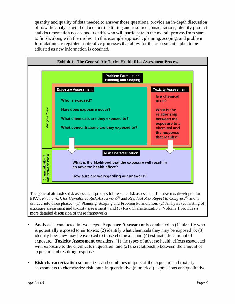
Exhibit 1. The General Air Toxics Health Risk Assessment Process
The general air toxics risk assessment process follows the risk assessment frameworks developed forEPA’s Framework for Cumulative Risk Assessment(1) and Residual Risk Report to Congress(2) and isdivided into three phases: (1) Planning, Scoping and Problem Formulation; (2) Analysis (consisting ofexposure assessment and toxicity assessment); and (3) Risk Characterization. Volume 1 provides amore detailed discussion of these frameworks.
• Analysis is conducted in two steps. Exposure Assessment is conducted to (1) identify whois potentially exposed to air toxics; (2) identify what chemicals they may be exposed to; (3)identify how they may be exposed to those chemicals; and (4) estimate the amount ofexposure. Toxicity Assessment considers: (1) the types of adverse health effects associatedwith exposure to the chemicals in question; and (2) the relationship between the amount ofexposure and resulting response.
• Risk characterization summarizes and combines outputs of the exposure and toxicityassessments to characterize risk, both in quantitative (numerical) expressions and qualitative
April 2004 Page 4
EPA is investigating whether it is possible todevelop a Tier 1 ecological risk assessmentmethodology to allow sources/facilities that emitsmall amounts of PB-HAP compounds todemonstrate that risk targets are met using simplelook-up tables or graphs. EPA also isinvestigating whether any HAPs pose ecologicalproblems in air at concentrations below thehuman-health based Reference Concentration(RfC). This resource document may be revisedto incorporate an example Tier 1 ecological riskassessment methodology and/or an exampleapproach for performing ecological assessmentsfor direct exposure to air toxics in ambient air.
(descriptive) statements. Specifically, chemical-specific dose-response toxicity informationis mathematically combined with modeled or monitored exposure estimates and otherinformation about how exposure occurs to give numbers that represent the potential for theexposure to cause an adverse health outcome.
Information about risk is extremely helpful to decision makers as they try to balance thecompeting needs of protecting public health, sustaining economic development, evaluatingissues of fairness and equity, and other factors specific to the laws and regulations controllingeach risk management decision. The approach described in this document also can be used tocompare risks from different exposures (e.g., the risk from breathing contaminated air comparedto the risk from drinking contaminated water). Risk assessment is already used by EPA todetermine the safety of foods containing pesticides, clean contaminated land and water bodies,regulate what chemicals can be imported into the United States, and set allowable limits onchemicals in our drinking water. Volume 1 of this series, the Technical Resource Manual,discusses the overall air toxics risk assessment process and the basic technical tools needed toperform these analyses. The Manual addresses both human health and ecological analyses. Italso provides a basic overview of the process of managing and communicating risk assessmentresults.
2.2 Facility/Source-Specific Ecological Assessment
When a specific set of air toxics that persistand which also may bioaccumulate orbiomagnify (PB-HAP compounds) arepresent in releases, the risk assessmentgenerally will need to include considerationof exposure pathways that involve depositionof air toxics onto soil, onto plants, and intowater; subsequent uptake by biota; andpotential exposures to ecological receptors(e.g., birds, fish, plants) via direct exposure tocontaminated media and/or indirect exposurethrough aquatic and terrestrial food chains. Air toxics ecological risk assessment is theprocess by which the risks of adverse impactsto ecological receptors associated withexposures to air toxics are estimated.
Congress has recognized the importance of protecting ecological receptors from adverse effectsresulting from exposure to air toxics. For example, Sections 112(f)(2) through (6) of the CAArequire EPA to promulgate standards beyond MACT when necessary to provide “an amplemargin of safety to protect public health” and to “prevent, considering costs, energy, safety, andother relevant factors, an adverse environmental effect” (note that the requirements of otherauthorities may vary). The major philosophical difference between ecological and health riskmanagement decision making is that health-based decisions intend to protect groups ofindividuals (e.g., population subgroups), whereas ecologically-based decisions intend to protectspecies and ecosystems.
April 2004 Page 5
Ecological risk assessment uses scientificprinciples and methods to answer the followingquestions, which are analogous to those forhuman health risk assessment:
• What receptors are exposed to air toxics?• What air toxics are they are exposed to?• How are they exposed (including directly and
via food chains)?• How much are they exposed to?• How dangerous are the specific chemicals?• How likely is it that exposed receptors will
suffer adverse impacts because of theexposures?
• How sure are we that our answers are correct?
The ecological risk assessment process also has three main phases that broadly correspond to thethree basic phases of the human health risk assessment methodology.
• Problem formulation, whichcorresponds to the planning, scoping, andproblem formulation phase of the humanhealth risk assessment methodology;
• Analysis, which corresponds to theanalysis phase of the human health riskassessment methodology and includes theexposure assessment and ecologicaleffects assessment steps; and
• Risk characterization, whichcorresponds to the risk characterizationphase of the human health risk assessmentmethodology.
2.3 Use of Site-Specific Risk Assessments in EPA’s Air Toxics Program
The results of any site-specific risk assessment can be used to support a number of activities,including:
• Development and implementation of source-specific standards and sector-based standards;
• Development and implementation of area-wide risk assessments and strategies developed bystate or local air pollution control agencies to address air toxics in urban areas;
• Implementation of national air toxics assessments (NATA) activities; and
• Development of education and outreach tools.
3.0 The Layout of This Resource Document
The remainder of Volume 2 is divided into three chapters:
Chapter II: Overview and Getting Started provides an overview of risk assessment anddescribes several important initial steps.
• Section 1 provides an introduction to Chapter II.
• Section 2 presents an overview of the risk assessment methodology, including the basicphases and steps (planning, scoping, and problem formulation; exposure assessment; toxicityassessment; and risk characterization).
April 2004 Page 6
• Section 3 introduces the concept of a tiered approach, starting with a relatively simple,health-protective screening analysis and continuing with more complex and realistic analysesas needed to answer specific assessment questions.
• Section 4 describes the initial planning, scoping, and problem formulation steps thatgenerally are followed prior to conducting the risk assessment. Three key elements arehighlighted: developing a conceptual model, developing an analysis plan, and determiningwhether multipathway analyses are needed.
• Section 5 describes a toxicity-weighted screening analysis that can be used to focus the riskanalysis on a smaller subset of HAPs that contribute the most to risk.
Chapter III: Inhalation Pathway Risk Assessment describes one set of methods andapproaches that could be used to conduct human health risk assessments for inhalationexposures.
• Section 1 provides an introduction to Chapter III.
• Section 2 provides an example of how to structure a tiered assessment approach (includingthe use of different models at different tiers) for the inhalation analysis.
• Section 3 provides an example of how to develop the emissions inventory for an inhalationanalysis.
• Section 4 describes an example of how to perform an inhalation toxicity assessment for bothchronic and acute exposures.
• Section 5 describes an example risk characterization for inhalation analyses.
• Section 6 describes an example structure for a Tier 1 assessment highlighting a focus on aprotective estimate of the location of the maximum exposed individual.
• Section 7 describes an example structure for a Tier 2 assessment highlighting a focus on amore realistic estimate of the highest individual risk in areas that people are believed tooccupy.
• Section 8 describes an example structure for a Tier 3 assessment, highlighting the use ofexposure modeling to assess variability and uncertainty in the activity patterns of the exposedpopulation.
Chapter IV: Multipathway Risk Assessment describes one set of methods and approaches forconducting human health and ecological risk assessments for exposure pathways that involvedeposition of PB-HAP compounds to soils and surface waters and subsequent uptake andingestion exposures.
• Section 1 provides an introduction to this Chapter IV.
April 2004 Page 7
This document focuses on EPA risk assessment methods and resources. Note that many stateand local governments have air toxics programs. For example, California has an existing healthrisk assessment methodology which has been scientifically peer reviewed and has gone throughextensive public comment http://www.oehha.ca.gov/air/hot_spots/index.html. State and localagencies may have existing methodologies that are acceptable for conducting facility/source-specific health risk assessments.
• Section 2 provides an example of how to structure a tiered assessment approach (includingthe use of different models at different tiers) for the inhalation analysis.
• Section 3 provides an example of how to develop the emissions inventory for a multipathwayanalysis.
• Section 4 describes an example structure for a tiered multipathway human health riskassessment for chronic exposures.
• Section 5 describes an example structure for a tiered ecological risk assessment.

April 2004 Page 8
(this page intentionally left blank)
April 2004 Page 9
Chapter II: Overview and Getting Started
1.0 Introduction
This chapter provides an overview of the methodology EPA uses to quantitatively predict humanhealth risks from emissions of HAPs at a specific facility or source in a source category. Itintroduces the tiered risk assessment process for facility-specific assessments. It also describesimportant steps in getting started, including planning, scoping, problem formulation, andconducting a toxicity-weighted emissions screening process to focus the analysis on the HAPs ofgreatest potential human health concern. Basic risk assessment concepts, principles, andmethods are described in more detail in Volume 1 of this series. The remainder of this chapter isdivided into four sections:
• Overview of Risk Assessment (Section 2);• Concept of Tiered Assessment (Section 3)• Planning, Scoping, and Problem Formulation (Section 4); and• Focusing on the Most Important HAPs (Section 5).
2.0 Overview of Risk Assessment and Risk Management
The site-specific risk assessment methodology follows the risk assessment frameworksestablished for EPA’s Framework for Cumulative Risk Assessment(1) and Residual Risk Report toCongress.(2) Volume 1 provides a more detailed discussion of these frameworks and theirrelationship to the general risk assessment paradigm established by the National Academy ofSciences (1983) and used throughout the federal government. The methodology includes thefollowing components (Exhibit 2):
• Planning, scoping, and problem formulation;• Analysis (consisting of exposure assessment and toxicity assessment); and• Risk characterization (including qualitative or quantitative uncertainty analysis).
Any risk assessment begins with planning and scoping. Properly planning and scoping the riskassessment at the beginning of the project is critical to the success of the overall effort. Planningand scoping focuses on a communication step among managers, assessors, and otherstakeholders regarding the purpose, scope, participants, approaches, and resources available forthe risk assessment.
Problem formulation generally is conducted by both risk assessors and risk managers andfocuses on two key products. The conceptual model identifies sources of emissions, HAPsemitted and emissions rates, the location of human and ecological receptors, potential exposurepathways/routes, and any areas (land or water) that have the potential to be contaminated fromdeposition of air toxics emitted from the facility/source. The conceptual model may be refinedas new information becomes available during the tiered assessment process. Risk assessors usethe study-specific conceptual model as a guide to help determine what types, amount, and qualityof data are needed for the study to answer the questions the risk assessment has set out toevaluate. The analysis plan describes the specific requirements and methods to be used to
April 2004 Page 10
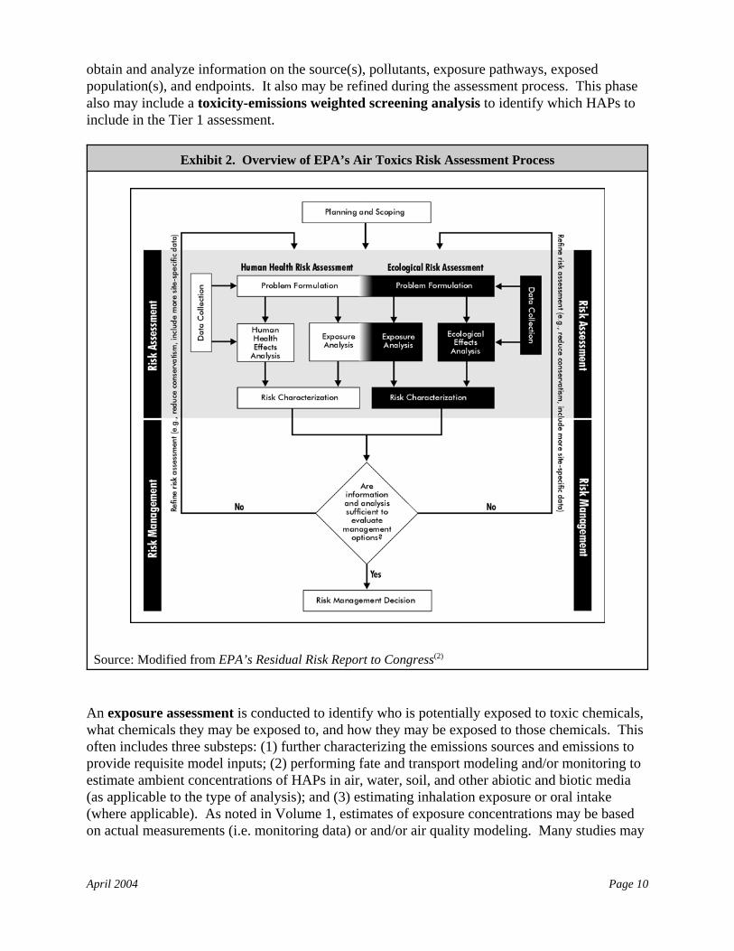
obtain and analyze information on the source(s), pollutants, exposure pathways, exposedpopulation(s), and endpoints. It also may be refined during the assessment process. This phasealso may include a toxicity-emissions weighted screening analysis to identify which HAPs toinclude in the Tier 1 assessment.
Exhibit 2. Overview of EPA’s Air Toxics Risk Assessment Process
Source: Modified from EPA’s Residual Risk Report to Congress(2)
An exposure assessment is conducted to identify who is potentially exposed to toxic chemicals,what chemicals they may be exposed to, and how they may be exposed to those chemicals. Thisoften includes three substeps: (1) further characterizing the emissions sources and emissions toprovide requisite model inputs; (2) performing fate and transport modeling and/or monitoring toestimate ambient concentrations of HAPs in air, water, soil, and other abiotic and biotic media(as applicable to the type of analysis); and (3) estimating inhalation exposure or oral intake(where applicable). As noted in Volume 1, estimates of exposure concentrations may be basedon actual measurements (i.e. monitoring data) or and/or air quality modeling. Many studies may
aDose-response values are numerical expressions of the relationship between a given level of exposure to anair toxic and adverse health impacts. The two most common toxicity values for inhalation exposures are the upper-bound inhalation unit risk estimates (IURs) for cancer effects and reference concentrations (RfCs) for noncancereffects (which include uncertainty factors). Chapter III, Section 4 provides a more detailed discussion of toxicityvalues.
April 2004 Page 11
benefit by using some combination of modeling and monitoring, because the two approaches canbe complementary.
The toxicity assessment component of the risk assessment process considers: (1) the types ofadverse health effects associated with exposure to the chemicals in question, and (2) therelationship between the amount of exposure and resulting response.
• Hazard identification is the process of determining whether exposure to a chemical cancause an increase in the incidence of an adverse health effect (e.g., cancer, birth defects), andthe nature and strength of the evidence for causation.
• Dose-response assessment is the process of quantitatively characterizing the relationshipbetween the dose of the contaminant and the incidence of adverse health effects in theexposed population. As information on dose at the site in the body where the responseoccurs is rarely available, various surrogates (dose metrics) are employed, often with theassistance of biologically-based pharmacokinetic or dosimetry models to predict the dosemetric from the inhalation exposure concentration or oral intake estimates. From thisquantitative dose-response relationship, dose-response values are derived for use in riskcharacterization.(a) Most toxicity assessments are based on studies in which toxicologistsexpose animals to chemicals in a laboratory and extrapolate the results to humans. For somechemicals, information from actual human exposures is available (usually from studies ofworkplace exposures).
The risk characterization phase integrates the exposure and toxicity assessments to estimaterisks. Cancer risk is expressed in numerical terms (e.g., 1×10⁻⁵ or 10 in a million) as theincremental chance an individual will develop cancer in their lifetime as a result of the exposure,and/or as the converse, the concentration corresponding to a particular level of risk. Noncancerhazard is expressed as a Hazard Quotient (HQ), the ratio of the estimated exposure to thenoncancer dose-response value. For the assessment of exposures to mixtures of multiplepollutants, a Hazard Index (HI, the sum of the HQs of each chemical in a mixture) may becalculated. The individual HQs may be summed separately for chemicals that affect the sametarget organ/organ system or act by similar toxicological processes (e.g., the sum of the HQs forall HAPs that produce liver disease as a critical effect). Such a metric is called a Target OrganSpecific Hazard Index (TOSHI). Ecological risk is often expressed as an ecological HI derivedin a manner analogous to the human health HI.
Uncertainty and variability are inherent characteristics of risk assessments, and therefore the riskcharacterization phase includes an analysis and presentation of uncertainty and variability. Airtoxics risk assessments make use of many different kinds of scientific concepts and data (e.g.,exposure, toxicity, epidemiology, ecology), all of which are used to characterize the expectedrisk in a particular environmental context. Informed use of reliable scientific information from
April 2004 Page 12
This document focuses on the modeling approach to estimating exposure. Ambient concentrationsobtained by monitoring can be incorporated into facility/source-specific risk assessments, generallyafter initial (Tier 1) assessments indicate a potential for risk. As noted in Volume 1:
• The scope of monitoring is necessarily limited (i.e., spatially, temporally, and in number ofpollutants measured) by resources;
• Monitoring cannot attribute exposures to sources;• Monitoring cannot estimate exposures below the detection limit;• Monitoring cannot predict the effects of various possible risk reduction options on future
exposures; and• Monitoring is therefore most effectively used to evaluate or further characterize modeled
concentrations and exposures.
Volume 1 and EPA’s NATA web site (http://www.epa.gov/ttn/atw/nata/draft6.html#secIV.B.i)provide detailed discussions of how monitoring can complement modeling in the exposure assessment.
many different sources is a central feature of the risk assessment process. Reliable informationmay or may not be available for many aspects of a risk assessment. Uncertainty and variabilityare inherent in the risk assessment process, and risk managers almost always must makedecisions using assessments that are not as definitive in all important areas as would bedesirable. Risk assessments also incorporate a variety of professional and science policyjudgments (e.g., which models to use, where to locate monitors, which toxicity studies to use asthe basis of developing dose-response values). Risk managers need to understand the strengthsand the limitations of each assessment to communicate this information to all participants,including the public.(3) Several techniques for assessing and describing uncertainty are describedmore fully in Volume I (see this endnote for several key references).(4)
Risk management refers to the regulatory and other actions taken to limit or control exposuresto a chemical. Risk management considers the quantitative and qualitative expressions of risk(along with attendant uncertainties) developed during the risk assessment, as well as a variety ofadditional information (e.g., the cost of reducing emissions or exposures, the statutory authorityto take regulatory actions, and the acceptability of control options) to reach a final decision.
3.0 Concept of Tiered Assessment
The human health risk assessment methodology may be based on several tiers of analysis,ranging from relatively simple, health-protective risk estimates based on limited information tocomplex, more realistic estimates involving more intensive data collection and calculations (seeExhibit 3).
April 2004 Page 13
Tier 1: Screening Level• Exposure = max offsite levels• Simple modeling• Low cost
Tier 2: Moderate Complexity• Exposure = residential air levels • More detailed modeling• Moderate cost
Tier 3: High Complexity• Complex exposure assessment• Detailed site-specific modeling• High cost
Incr
easi
ng C
ompl
exity
/Res
ourc
e R
equi
rem
ents
Cha
ract
eriz
atio
n of
Var
iabi
lity
and/
or U
ncer
tain
ty
Decision-making cycle: Evaluating the adequacy of the risk assessment and the value of additional complexity/level of effort
Decision-making cycle: Evaluating the adequacy of the risk assessment and the value of additional complexity/level of effort
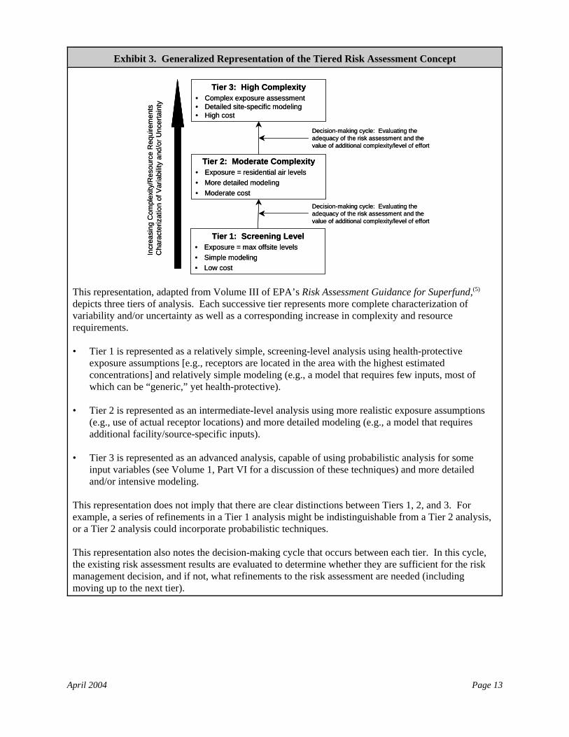
Exhibit 3. Generalized Representation of the Tiered Risk Assessment Concept
This representation, adapted from Volume III of EPA’s Risk Assessment Guidance for Superfund,(5)
depicts three tiers of analysis. Each successive tier represents more complete characterization ofvariability and/or uncertainty as well as a corresponding increase in complexity and resourcerequirements.
• Tier 1 is represented as a relatively simple, screening-level analysis using health-protectiveexposure assumptions [e.g., receptors are located in the area with the highest estimatedconcentrations] and relatively simple modeling (e.g., a model that requires few inputs, most ofwhich can be “generic,” yet health-protective).
• Tier 2 is represented as an intermediate-level analysis using more realistic exposure assumptions(e.g., use of actual receptor locations) and more detailed modeling (e.g., a model that requiresadditional facility/source-specific inputs).
• Tier 3 is represented as an advanced analysis, capable of using probabilistic analysis for someinput variables (see Volume 1, Part VI for a discussion of these techniques) and more detailedand/or intensive modeling.
This representation does not imply that there are clear distinctions between Tiers 1, 2, and 3. Forexample, a series of refinements in a Tier 1 analysis might be indistinguishable from a Tier 2 analysis,or a Tier 2 analysis could incorporate probabilistic techniques.
This representation also notes the decision-making cycle that occurs between each tier. In this cycle,the existing risk assessment results are evaluated to determine whether they are sufficient for the riskmanagement decision, and if not, what refinements to the risk assessment are needed (includingmoving up to the next tier).
April 2004 Page 14
A health-protective exposure estimate is anestimate based on assumptions about exposure(e.g., release, atmospheric dispersion, contactwith contaminated air) that would result in areasonable maximum level of exposure. It isnot necessarily the highest level of exposurethat theoretically could occur. The term“conservative” is often used synonymouslywith “health protective.”
The example Tiered approach presented in this document illustrates how an iterative riskassessment process can be used to first screen out facilities/sources that represent a relatively lowrisk and then focus the risk assessment on the sources and HAPs that may require emissionsreduction actions. Tier 1 and Tier 2 analyses generally are an appropriate basis for deciding not totake any action or what to leave out of the next tier of analysis. Significant emissions reductionactions are likely to need a Tier 3 analysis of the specific sources and HAPs that drive the exposureand risk.
This document presents a three-tiered approachand describe the types of models andassumptions that would be consistent with theconservativeness of these tiers. This discussionis modeled on EPA’s general framework forassessing residual risk pursuant to section112(f) of the CAA. This resource document ismeant to provide an example and is notintended to prescribe a specific approach thatmust be used by EPA or others in a particularrisk assessment activity. In particular, variousmodifications to this tiered approach may be both cost-effective and appropriate, such asadding intermediate-level tiers that incorporate some features of the higher and lower tiers, orconducting iterative, more refined analyses within a given tier.
Facility-specific assessments by regulatory agencies are often designed to answer the question: “Is the estimated risk from a facility or source category low enough to support a finding that it isof negligible regulatory concern?” If a simple, health-protective Tier 1 assessment provides a“yes” answer, there may be no need for regulatory action or further assessment. If the answer is“no,” the risk manager will need to decide whether to consider a regulatory response or to refinethe assessment at a higher tier. If a higher-tier assessment is performed, the decision process isrepeated.
For example, a Tier 1 analysis might consist of screening-level dispersion modeling usingSCREEN3. The Tier 1 analysis would typically provide a single estimate of maximum ambientair concentration that would be used to estimate inhalation risk based on an assumption that themaximum exposed individual could reside at the offsite location of maximum concentration,whether or not a person actually lived there. A Tier 2 analysis might then use the more refinedHuman Exposure Model, version 3 (HEM-3). HEM-3 uses the Industrial Source ComplexShort-Term, version 3 (ISCST3) to provide spatially-resolved air concentrations. It combinesconcentration data with U.S. Census Bureau population data (2000 census) to estimate risk andhazard for the population in the most-exposed Census block. A Tier 3 analysis might coupledispersion modeling using ISCST3 with exposure modeling using Trim.ExpoInhalation to estimaterisk and hazard for hypothetical individuals used to represent the exposed population based oncombinations of demographic characteristics and activity patterns. A Tier 3 approach might alsoadd a probabilistic exposure model to quantify the effects of variable human behavior on theexposure and risk estimates. Because the lower tier analyses are generally designed to be more
April 2004 Page 15
Determination of appropriate tiers may depend on the purpose of and regulatory context for the riskassessment. For example, if the regulatory authority for a risk management decision does notinclude consideration of population risk, a Tier 2 analysis might incorporate the use of a morerefined air quality model to more accurately estimate maximum impact. Choice of a particularmodel to use within any Tier also may depend on facility/source-specific factors. For example, ifdownwash is particularly important at a given facility, a model other than ISCST3 may be moreappropriate at Tier 2. If consideration of potential future land use is important, a model based oncurrent land use (e.g., HEM-3) may not be the appropriate tool. Finally, the assessment may needto comply with specific S/L/T guidelines for how risk analyses should be conducted.
health-protective, a facility-specific assessment can be performed at the lowest tier thatdemonstrates that applicable low-risk targets are met.
4.0 Planning, Scoping, and Problem Formulation
Volume I of this reference library discusses in detail the general planning, scoping, and problemformulation process, including identifying the specific concerns; determining who will beinvolved in the risk assessment process (including the risk managers, risk assessment technicalteam, and stakeholders); communicating the purpose and scope of the risk assessment; anddetermining what resources are available for the risk assessment. Volume I also provides adetailed discussion of the problem formulation process, including developing a study-specificconceptual model and developing the important plans that will guide the risk assessment,including the analysis plan, and quality-related plans such as the Quality Assurance Project Plan(QAPP).
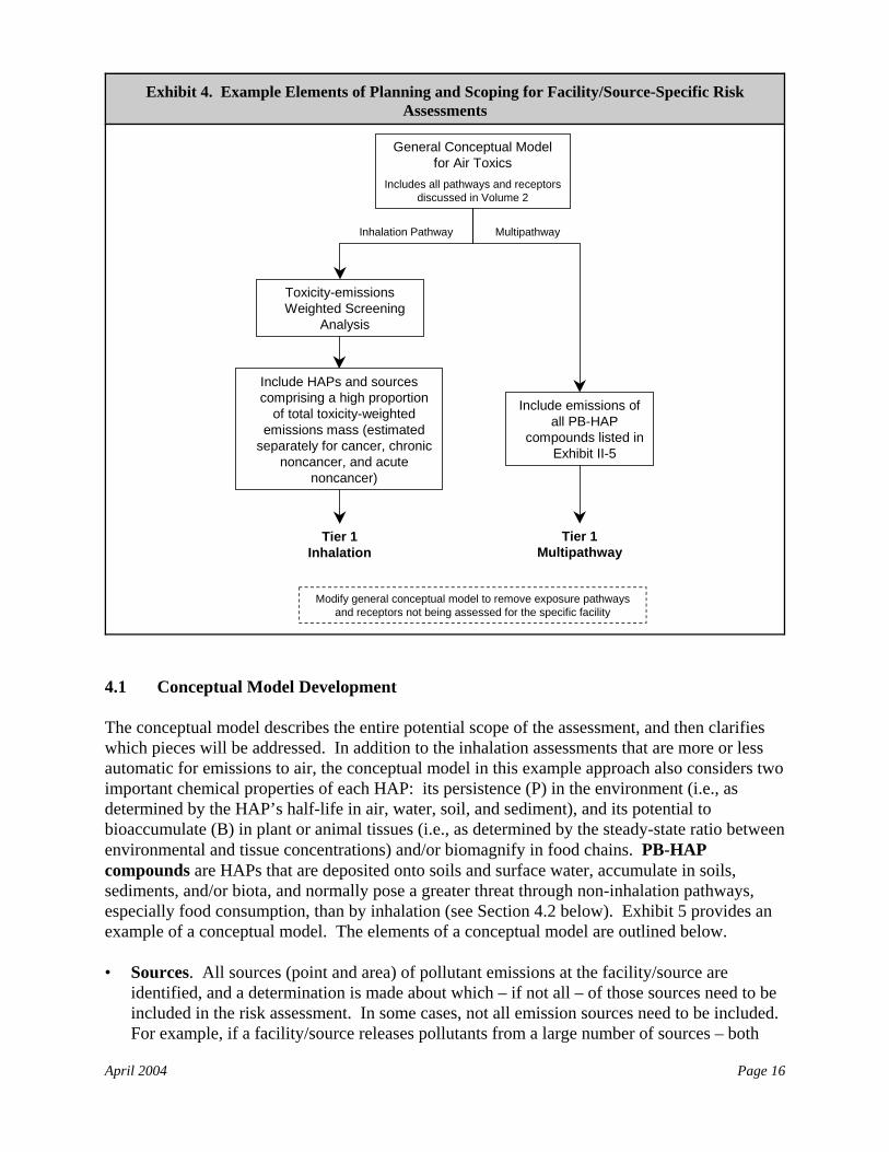
This section does not repeat the general discussion provided in Volume 1. Instead, it focuses ontwo aspects of planning, scoping, and problem formulation that are particularly important forfacility/source-specific air toxics risk assessments (Exhibit 4): developing the conceptual model(Section 4.1); and determining whether multipathway analyses (human health ingestion and/orecological) are applicable (Section 4.2).
Note that planning, scoping, and problem formulation activities generally continue throughoutthe risk assessment as new information is learned. The specific details of some activities alsowill vary depending on which type of analysis (i.e., human health-inhalation, human health-multipathway, ecological) and which tier of analysis is being performed.
April 2004 Page 16
Include HAPs and sources comprising a high proportion
of total toxicity-weighted emissions mass (estimated
separately for cancer, chronic noncancer, and acute
noncancer)
Include emissions of all PB-HAP
compounds listed in Exhibit II-5
Modify general conceptual model to remove exposure pathways and receptors not being assessed for the specific facility
General Conceptual Model for Air Toxics
Includes all pathways and receptors discussed in Volume 2
Toxicity-emissions Weighted Screening
Analysis
Tier 1Inhalation
Tier 1Multipathway
Inhalation Pathway Multipathway
Exhibit 4. Example Elements of Planning and Scoping for Facility/Source-Specific RiskAssessments
4.1 Conceptual Model Development
The conceptual model describes the entire potential scope of the assessment, and then clarifieswhich pieces will be addressed. In addition to the inhalation assessments that are more or lessautomatic for emissions to air, the conceptual model in this example approach also considers twoimportant chemical properties of each HAP: its persistence (P) in the environment (i.e., asdetermined by the HAP’s half-life in air, water, soil, and sediment), and its potential tobioaccumulate (B) in plant or animal tissues (i.e., as determined by the steady-state ratio betweenenvironmental and tissue concentrations) and/or biomagnify in food chains. PB-HAPcompounds are HAPs that are deposited onto soils and surface water, accumulate in soils,sediments, and/or biota, and normally pose a greater threat through non-inhalation pathways,especially food consumption, than by inhalation (see Section 4.2 below). Exhibit 5 provides anexample of a conceptual model. The elements of a conceptual model are outlined below.
• Sources. All sources (point and area) of pollutant emissions at the facility/source areidentified, and a determination is made about which – if not all – of those sources need to beincluded in the risk assessment. In some cases, not all emission sources need to be included. For example, if a facility/source releases pollutants from a large number of sources – both
April 2004 Page 17
While many facility/source-specific riskassessments focus on current land use, it may behelpful to assess risks associated with potentialfuture land use. Risk estimates based on currentconditions at the facility/source and current landuse could change if conditions at thefacility/source change (e.g., one process isreplaced by another) and/or land use changes(e.g., a housing development is built on currentlyundeveloped land).
large and small – the toxicity-weighted screening analysis (TWSA) may be used to determinewhich sources release negligible amounts of HAPs or low toxicity pollutants that might beexcluded from modeling (see Section 5 below). If data are readily available for emissionsfrom all sources, however, the risk assessor may choose to use those data in all tiers ofanalyses.
• Stressors. All HAPs released from the sources are identified. It also is helpful at this pointto characterize emissions from the sources and identify applicable dose-response values inorder to perform TWSA (described in Section 5). Additional information on characterizingemissions and identifying dose-response values is provided in Section 5 below.
• Exposure Pathways/Media/Routes. Potential exposure pathways/routes by which theidentified receptors can be exposed to the emitted HAPs are identified. The inhalationpathway commonly is included for all facility-specific assessments. Additional exposurepathways/routes, such as ingestion of animal and vegetable products raised on farms (humanhealth), or pathways of ecological exposure, may be performed if PB-HAP compounds arepresent in emissions.
• Receptors. Human and ecologicalreceptors that are potentially exposed tothe emitted HAPs are identified, located,and characterized. This includes all areas(land or water) that have the potential tobe contaminated from deposition of airtoxics emitted from the facility/source. Special ecological receptors such asendangered/threatened species orwetlands are identified. The conceptualmodel indicates areas where themaximum exposures are expected.
• Endpoints. The specific human health and ecological endpoints of concern for the emittedHAPs are identified, along with specific target organs.
• Metrics. The specific HAP-specific and cumulative metrics used to estimate risk/hazard(e.g., cancer type, weight of evidence, target-organ-specific hazard index) are identified,along with how they will be characterized for the exposed population (e.g., central tendency,high-end, distributions).
Volume I (Chapter 6) of this reference library provides a more detailed discussion of how toperform these important steps.
April 2004 Page 18
Etc.CNS Hazard Index
zBlood Hazard Index
Possible Carcinogens
Sources
Stressors
Pathways/Media
Routes
Receptors
Endpoints
Metrics
Point Sources
ABC Facility
NonpointSources
Volume Sources
PB-HAPsOther persistent air toxics
HAPsOther air toxics
Outdoor airIndoor air
microenvironments Soil FoodWater
Other Sources
Inhalation Ingestion Other (e.g., dermal)
General Population
Hispanic
African American
Native American
Asian American
Young Children
Pregnant Women
ElderlyWhite Other Other
Cancers Respiratory Blood Liver KidneyCNS Cardiovascular Other
Distribution of high-end cancer risk estimates
Estimated number of people within specified
cancer risk ranges
Estimated number of
cancer cases
Known Carcinogens
Probable Carcinogens
Respiratory System Hazard Index
Distribution of estimated
HI values
Estimated number of people within specified
ranges of HI values
Ecological Receptors
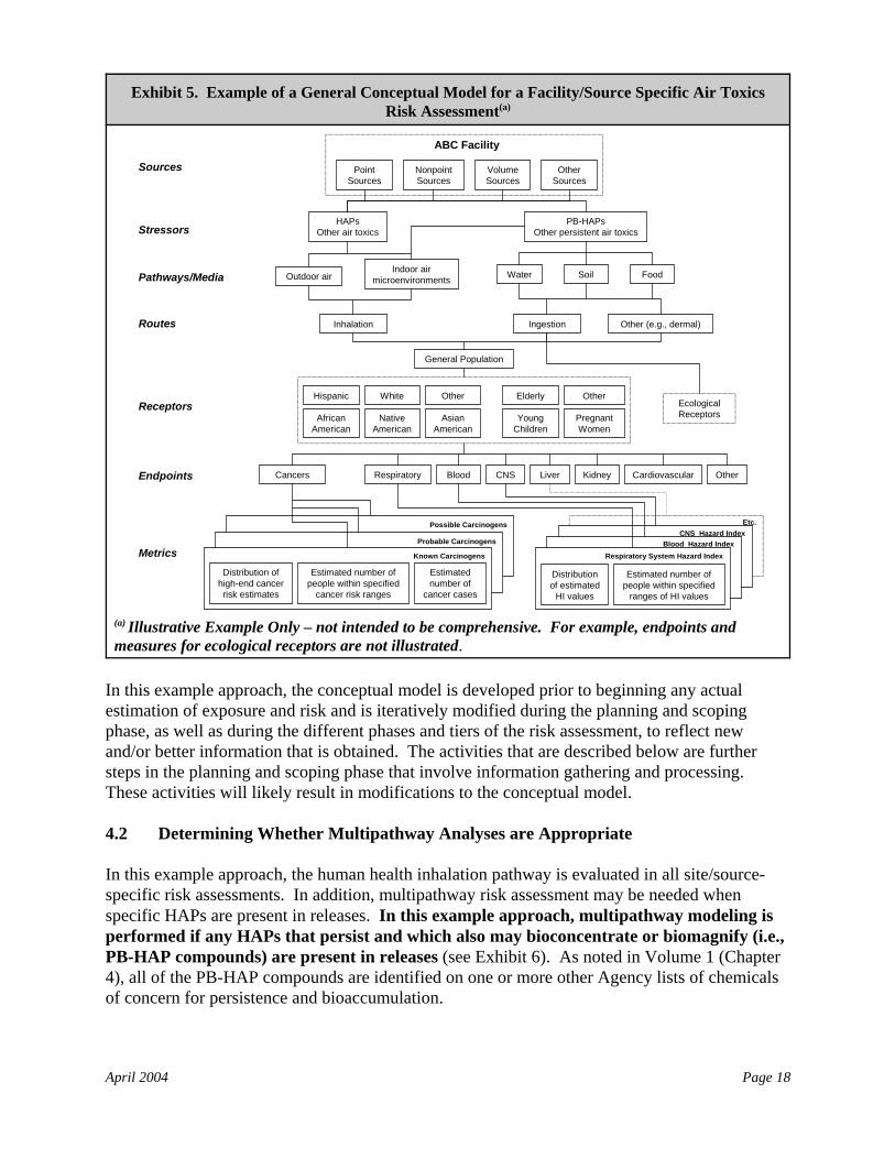
Exhibit 5. Example of a General Conceptual Model for a Facility/Source Specific Air ToxicsRisk Assessment(a)
(a) Illustrative Example Only – not intended to be comprehensive. For example, endpoints andmeasures for ecological receptors are not illustrated.
In this example approach, the conceptual model is developed prior to beginning any actualestimation of exposure and risk and is iteratively modified during the planning and scopingphase, as well as during the different phases and tiers of the risk assessment, to reflect newand/or better information that is obtained. The activities that are described below are furthersteps in the planning and scoping phase that involve information gathering and processing. These activities will likely result in modifications to the conceptual model.
4.2 Determining Whether Multipathway Analyses are Appropriate
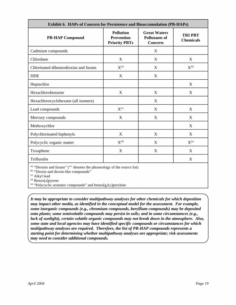
In this example approach, the human health inhalation pathway is evaluated in all site/source-specific risk assessments. In addition, multipathway risk assessment may be needed whenspecific HAPs are present in releases. In this example approach, multipathway modeling isperformed if any HAPs that persist and which also may bioconcentrate or biomagnify (i.e.,PB-HAP compounds) are present in releases (see Exhibit 6). As noted in Volume 1 (Chapter4), all of the PB-HAP compounds are identified on one or more other Agency lists of chemicalsof concern for persistence and bioaccumulation.
April 2004 Page 19
It may be appropriate to consider multipathway analyses for other chemicals for which depositionmay impact other media, as identified in the conceptual model for the assessment. For example,some inorganic compounds (e.g., chromium compounds, beryllium compounds) may be depositedonto plants; some semivolatile compounds may persist in soils; and in some circumstances (e.g.,lack of sunlight), certain volatile organic compounds may not break down in the atmosphere. Also,some state and local agencies may have identified specific compounds or circumstances for whichmultipathway analyses are required. Therefore, the list of PB-HAP compounds represents astarting point for determining whether multipathway analyses are appropriate; risk assessmentsmay need to consider additional compounds.
Exhibit 6. HAPs of Concern for Persistence and Bioaccumulation (PB-HAPs)
PB-HAP CompoundPollution
PreventionPriority PBTs
Great WatersPollutants of
Concern
TRI PBTChemicals
Cadmium compounds X
Chlordane X X X
Chlorinated dibenzodioxins and furans X(a) X X(b)
DDE X X
Heptachlor X
Hexachlorobenzene X X X
Hexachlorocyclohexane (all isomers) X
Lead compounds X(c) X X
Mercury compounds X X X
Methoxychlor X
Polychlorinated biphenyls X X X
Polycyclic organic matter X(d) X X(e)
Toxaphene X X X
Trifluralin X(a) “Dioxins and furans” (“” denotes the phraseology of the source list)(b) “Dioxin and dioxin-like compounds”(c) Alkyl lead(d) Benzo[a]pyrene(e) “Polycyclic aromatic compounds” and benzo[g,h,i]perylene
April 2004 Page 20
This example TWSA approach uses a cutoff of99 percent of total toxicity-weighted emissions. This is not intended as a suggested value, asothers (e.g., 90 or 95 percent) may be appropriatefor focusing a given risk assessment on the subsetof HAPs that are likely to drive the riskmanagement decision.
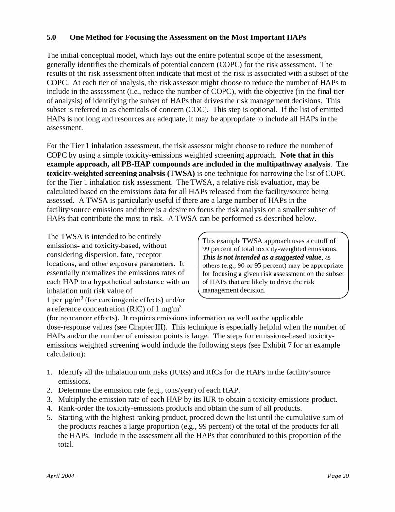
5.0 One Method for Focusing the Assessment on the Most Important HAPs
The initial conceptual model, which lays out the entire potential scope of the assessment,generally identifies the chemicals of potential concern (COPC) for the risk assessment. Theresults of the risk assessment often indicate that most of the risk is associated with a subset of theCOPC. At each tier of analysis, the risk assessor might choose to reduce the number of HAPs toinclude in the assessment (i.e., reduce the number of COPC), with the objective (in the final tierof analysis) of identifying the subset of HAPs that drives the risk management decisions. Thissubset is referred to as chemicals of concern (COC). This step is optional. If the list of emittedHAPs is not long and resources are adequate, it may be appropriate to include all HAPs in theassessment.
For the Tier 1 inhalation assessment, the risk assessor might choose to reduce the number ofCOPC by using a simple toxicity-emissions weighted screening approach. Note that in thisexample approach, all PB-HAP compounds are included in the multipathway analysis. Thetoxicity-weighted screening analysis (TWSA) is one technique for narrowing the list of COPCfor the Tier 1 inhalation risk assessment. The TWSA, a relative risk evaluation, may becalculated based on the emissions data for all HAPs released from the facility/source beingassessed. A TWSA is particularly useful if there are a large number of HAPs in thefacility/source emissions and there is a desire to focus the risk analysis on a smaller subset ofHAPs that contribute the most to risk. A TWSA can be performed as described below.
The TWSA is intended to be entirelyemissions- and toxicity-based, withoutconsidering dispersion, fate, receptorlocations, and other exposure parameters. Itessentially normalizes the emissions rates ofeach HAP to a hypothetical substance with aninhalation unit risk value of 1 per µg/m3 (for carcinogenic effects) and/ora reference concentration (RfC) of 1 mg/m3
(for noncancer effects). It requires emissions information as well as the applicabledose-response values (see Chapter III). This technique is especially helpful when the number ofHAPs and/or the number of emission points is large. The steps for emissions-based toxicity-emissions weighted screening would include the following steps (see Exhibit 7 for an examplecalculation):
1. Identify all the inhalation unit risks (IURs) and RfCs for the HAPs in the facility/sourceemissions.
2. Determine the emission rate (e.g., tons/year) of each HAP.3. Multiply the emission rate of each HAP by its IUR to obtain a toxicity-emissions product.4. Rank-order the toxicity-emissions products and obtain the sum of all products.5. Starting with the highest ranking product, proceed down the list until the cumulative sum of
the products reaches a large proportion (e.g., 99 percent) of the total of the products for allthe HAPs. Include in the assessment all the HAPs that contributed to this proportion of thetotal.
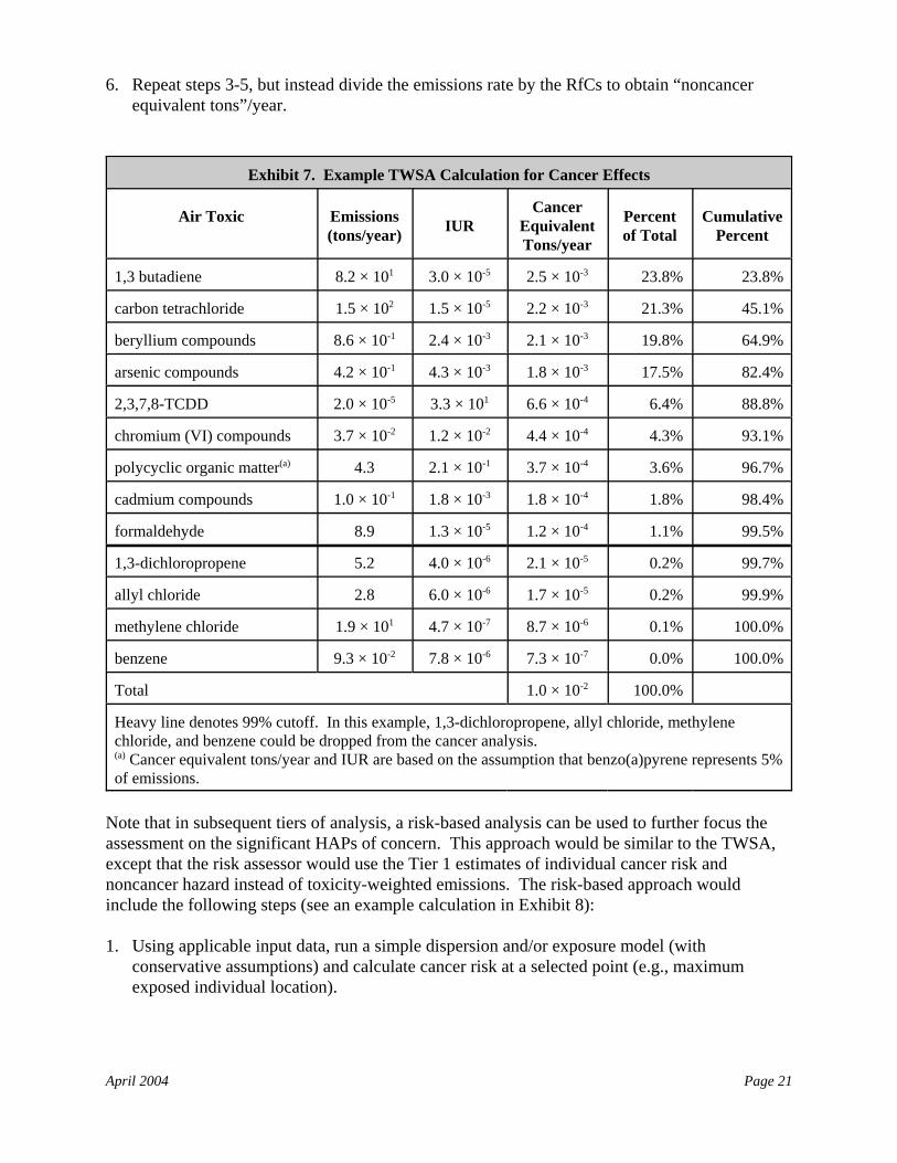
April 2004 Page 21
6. Repeat steps 3-5, but instead divide the emissions rate by the RfCs to obtain “noncancerequivalent tons”/year.
Exhibit 7. Example TWSA Calculation for Cancer Effects
Air Toxic Emissions(tons/year) IUR
CancerEquivalentTons/year
Percentof Total
CumulativePercent
1,3 butadiene 8.2 × 101 3.0 × 10⁻⁵ 2.5 × 10⁻³ 23.8% 23.8%
carbon tetrachloride 1.5 × 10² 1.5 × 10⁻⁵ 2.2 × 10⁻³ 21.3% 45.1%
beryllium compounds 8.6 × 10⁻¹ 2.4 × 10⁻³ 2.1 × 10⁻³ 19.8% 64.9%
arsenic compounds 4.2 × 10⁻¹ 4.3 × 10⁻³ 1.8 × 10⁻³ 17.5% 82.4%
2,3,7,8-TCDD 2.0 × 10⁻⁵ 3.3 × 101 6.6 × 10⁻⁴ 6.4% 88.8%
chromium (VI) compounds 3.7 × 10⁻² 1.2 × 10⁻² 4.4 × 10⁻⁴ 4.3% 93.1%
polycyclic organic matter(a) 4.3 2.1 × 10⁻¹ 3.7 × 10⁻⁴ 3.6% 96.7%
cadmium compounds 1.0 × 10⁻¹ 1.8 × 10⁻³ 1.8 × 10⁻⁴ 1.8% 98.4%
formaldehyde 8.9 1.3 × 10⁻⁵ 1.2 × 10⁻⁴ 1.1% 99.5%
1,3-dichloropropene 5.2 4.0 × 10⁻⁶ 2.1 × 10⁻⁵ 0.2% 99.7%
allyl chloride 2.8 6.0 × 10⁻⁶ 1.7 × 10⁻⁵ 0.2% 99.9%
methylene chloride 1.9 × 101 4.7 × 10⁻⁷ 8.7 × 10⁻⁶ 0.1% 100.0%
benzene 9.3 × 10⁻² 7.8 × 10⁻⁶ 7.3 × 10⁻⁷ 0.0% 100.0%
Total 1.0 × 10⁻² 100.0%
Heavy line denotes 99% cutoff. In this example, 1,3-dichloropropene, allyl chloride, methylenechloride, and benzene could be dropped from the cancer analysis.(a) Cancer equivalent tons/year and IUR are based on the assumption that benzo(a)pyrene represents 5%of emissions.
Note that in subsequent tiers of analysis, a risk-based analysis can be used to further focus theassessment on the significant HAPs of concern. This approach would be similar to the TWSA,except that the risk assessor would use the Tier 1 estimates of individual cancer risk andnoncancer hazard instead of toxicity-weighted emissions. The risk-based approach wouldinclude the following steps (see an example calculation in Exhibit 8):
1. Using applicable input data, run a simple dispersion and/or exposure model (withconservative assumptions) and calculate cancer risk at a selected point (e.g., maximumexposed individual location).
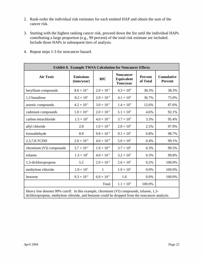
April 2004 Page 22
2. Rank-order the individual risk estimates for each emitted HAP and obtain the sum of thecancer risk.
3. Starting with the highest ranking cancer risk, proceed down the list until the individual HAPscontributing a large proportion (e.g., 99 percent) of the total risk estimate are included. Include those HAPs in subsequent tiers of analysis.
4. Repeat steps 1-3 for noncancer hazard.
Exhibit 8. Example TWSA Calculation for Noncancer Effects
Air Toxic Emissions(tons/year) RfC
NoncancerEquivalentTons/year
Percentof Total
CumulativePercent
beryllium compounds 8.6 × 10⁻¹ 2.0 × 10⁻⁵ 4.3 × 10⁴ 38.3% 38.3%
1,3 butadiene 8.2 × 101 2.0 × 10⁻³ 4.1 × 10⁴ 36.7% 75.0%
arsenic compounds 4.2 × 10⁻¹ 3.0 × 10⁻⁵ 1.4 × 10⁴ 12.6% 87.6%
cadmium compounds 1.0 × 10⁻¹ 2.0 × 10⁻⁵ 5.1 × 10³ 4.6% 92.1%
carbon tetrachloride 1.5 × 10² 4.0 × 10⁻² 3.7 × 10³ 3.3% 95.4%
allyl chloride 2.8 1.0 × 10⁻³ 2.8 × 10³ 2.5% 97.9%
formaldehyde 8.9 9.8 × 10⁻³ 9.1 × 10² 0.8% 98.7%
2,3,7,8-TCDD 2.0 × 10⁻⁵ 4.0 × 10⁻⁸ 5.0 × 10² 0.4% 99.1%
chromium (VI) compounds 3.7 × 10⁻² 1.0 × 10⁻⁴ 3.7 × 10² 0.3% 99.5%
toluene 1.3 × 10² 4.0 × 10⁻¹ 3.2 × 10² 0.3% 99.8%
1,3-dichloropropene 5.2 2.0 × 10⁻² 2.6 × 10² 0.2% 100.0%
methylene chloride 1.9 × 101 1 1.9 × 101 0.0% 100.0%
benzene 9.3 × 10⁻² 6.0 × 10⁻² 1.6 0.0% 100.0%
Total 1.1 × 10⁵ 100.0%
Heavy line denotes 99% cutoff. In this example, chromium (VI) compounds, toluene, 1,3-dichloropropene, methylene chloride, and benzene could be dropped from the noncancer analysis.
April 2004 Page 23
The three-tier approach described in this chapteris only one of a number of potential paradigmsthat may be appropriate and considered.
Chapter III: Inhalation Pathway Risk Assessment
1.0 Introduction
This chapter describes an example three-tiered approach to conducting site-specifichuman health-inhalation risk assessments forair toxics. The tiers range from a relativelysimple, health-protective screening analysis(Tier 1) to a complex probabilistic assessment (Tier 3). A risk assessor may decide to completeonly the lowest-tier analysis that fits the purpose of the assessment (e.g., to determine that afacility’s cumulative risk is lower than a risk manager’s level of concern). Conversely, anassessor may choose not to complete a lower-tier analysis before completing a higher-tieranalysis (e.g., the risk assessor could go directly to Tier 3).
The discussion in this chapter is divided into the following sections:
• Tiered Approach and Models Used (Section 2);• Developing the Emissions Inventory for an Inhalation Analysis (Section 3);• Toxicity Assessment (Section 4);• Risk Characterization for Inhalation Exposures (Section 5);• Tier 1 Inhalation Analysis (Section 6);• Tier 2 Inhalation Analysis (Section 7); and• Tier 3 Inhalation Analysis (Section 8).
2.0 Tiered Approach and Models Used
This example inhalation risk assessment methodology includes three tiers of analysis, each withexample models for dispersion, exposure, and risk (see Exhibit 9).
• Tier 1 would use a model like SCREEN3, which is a screening-level Gaussian dispersionmodel that estimates an hourly maximum ambient concentration based on hourly emissionrates. A relatively large degree of conservatism is incorporated in the SCREEN modelingprocedure to provide reasonable assurance that maximum concentrations will not beunderestimated.(6) Example default SCREEN3 inputs are identified for use in the absence offacility/source-specific data and are based on health-protective assumptions. The key outputis an estimate of the highest modeled offsite concentration per model run, which is used as asurrogate for exposure. This point may be referred to as the point of maximum exposedindividual (MEI). This concentration is combined with inhalation dose-response values(either for individual HAPs, or for HAPs combined by toxicity weighting) to calculate anestimate of the cumulative cancer risk and noncancer hazard to the most exposed individual. Note that SCREEN3 predicts 1-hour concentrations and requires a conversion factor in orderto do the risk assessment for chronic effects (see Section 6.2.1 below).
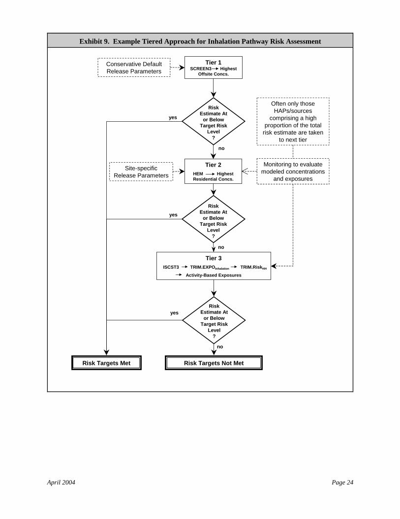
April 2004 Page 24
yes
no
yes
no
no
Risk Targets Met Risk Targets Not Met
yes
RiskEstimate At
or BelowTarget Risk
Level?
RiskEstimate At
or BelowTarget Risk
Level?
RiskEstimate At
or BelowTarget Risk
Level?
Often only those HAPs/sources
comprising a high proportion of the total
risk estimate are taken to next tier
Conservative Default Release Parameters
Site-specific Release Parameters
Tier 1SCREEN3 Highest
Offsite Concs.
Tier 2HEM Highest Residential Concs.
Tier 3ISCST3 TRIM.EXPOInhalation TRIM.RiskHH
Activity-Based Exposures
Monitoring to evaluate modeled concentrations
and exposures
Exhibit 9. Example Tiered Approach for Inhalation Pathway Risk Assessment
April 2004 Page 25
Key Locations for Estimating Chronic EC
• Point of maximum modeled concentration. The location where the maximum modeledambient concentration occurs, regardless ofwhether there is a person there or not. Thiswould provide a health-protective estimate ofexposure unless someone actually lives there. This point may be referred to as the point ofthe maximum exposed individual (MEI).
• Point of maximum modeled concentrationat an actual receptor location. Thepopulated location with the highest modeledambient concentration. This location may bean actual residence, a location within a Censusblock, or some other populated area. In somecases the risk assessor may decide to considerfuture residential use. The concentration maybe interpolated between unpopulated values. This point may be referred to as the point ofthe maximum individual risk (MIR).
• Tier 2 would use a model like the HumanExposure Model (HEM-3).(7) HEM-3incorporates the Industrial SourceComplex-Short Term (ISCST3) model,which is a more advanced Gaussiandispersion model that provides hourlyestimates of ambient concentrations bymodeling hourly emissions andmeteorology. The focus in Tier 2 is onthe maximum concentration to which anindividual is exposed (i.e., a person whoresides at the point of maximumexposure). This point may be referred toas the point of the maximum individualrisk (MIR). This is done within HEM-3using the internal point of the Censusblock with the highest modeled exposureor risk. It may be appropriate to consideravailable ambient air measurement data orconduct monitoring at Tier 2 to evaluateor further characterize modeledconcentrations at specific receptorlocations.
• Tier 3 would use a model like the ISCST3 model for ambient concentration estimates, butwould also incorporate an exposure model like TRIM.ExpoInhalation to provide a more realisticestimate of individual exposures. Tier 3 would also use a model like TRIM.RiskHH for riskcalculations. ISCST3 uses facility/source-specific source and meteorology data and providesspatially-resolved air concentrations at receptor locations. These concentrations (and/ormonitoring data) are used as inputs to TRIM.ExpoInhalation, which are used to calculateexposure to a set of hypothetical individuals, taking into account human activity patterns. TRIM.RiskHH combines the exposure estimates with dose-response values to calculate morerefined estimates of inhalation cancer risk and noncancer hazards that account for individualdifferences in daily activities, including where people live and work within the assessmentarea. As with Tier 2, monitoring data may be helpful for evaluating the estimated ambientair concentrations (e.g., from ISCST3). Additional measurements (e.g., indoor and outdoorconcentrations in specific locations where people live and work), as available, may be usefulin evaluating the exposure modeling component.
As noted earlier, other models may be appropriate for these tiers (e.g., AERMOD could beused at Tier 2).
April 2004 Page 26
Overview of Models Cited in This Example Approach
Air Quality Models
SCREEN3. SCREEN3 is a screening-level Gaussian dispersion model that estimates an hourlymaximum ambient concentration based on hourly emission rates. Short-term concentration results areused to estimate maximum annual averages via conversion factors that account for meteorologicalvariation and the type of process that produces the emissions. Results are not direction-specific (i.e.,wind direction is not taken into account). SCREEN3 calculates ambient concentrations assuming nodeposition or atmospheric reactions, “worst-case” generic meteorological conditions, and flat terrain. Data requirements are relatively low. For example, SCREEN3 uses facility/source-specific data (e.g.,stack height, diameter, flow rate, downwash) but does not use facility/source-specific meteorologydata. Data processing requirements are low; it is easy to use for quick assessment of a single facility orsource. SCREEN3 does not estimate deposition rates. SCREEN 3 is available at(http://www.epa.gov/ttn/scram/).(8)
Industrial Source Complex - Short Term (ISCST3). ISCST3 is a more advanced Gaussiandispersion model that provides hourly estimates of ambient concentrations by modeling hourlyemissions and meteorology. The model includes removal effects for wet and dry deposition flux forany locations specified by the user. Data requirements are higher than for SCREEN3. For example,ISCST3 requires hourly, site-specific, processed meteorological data; and physical characteristics ofemissions. Terrain information is optional. ISCST3 can accommodate variable emission rates. Moreexpertise (e.g., specific technical and computer skills) is required to use ISCST3. Unlike SCREEN3,ISCST3 estimates annual concentrations by integrating the hourly concentrations (i.e., no multiplier isused). The ISC model is available at (http://www.epa.gov/ttn/scram/).(9)
Exposure and Risk Models
Human Exposure Model (HEM-3). HEM-3 is designed to screen major stationary sources of airpollutant emissions efficiently, ranking the sources according to the potential cancer risks andnoncancer hazard associated with long-term (annual) average exposure concentrations. The currentversion is implemented on a Windows platform for ease of use. HEM-3 contains the Gaussianatmospheric dispersion model ISCST3 (with included meteorological data), and U.S. Census Bureaupopulation data (2000) at the Census block level. A limited amount of source data are required asmodel inputs (e.g., pollutant emission rates, facility/source location, height of the emission release,stack gas exit velocity, stack diameter, temperature of the off-gases, pollutant properties and sourcelocation). HEM-3 estimates the magnitude and distribution of ambient air concentrations of pollutantin the vicinity of each source. The model usually estimates these concentrations within a radialdistance of 50 kilometers (30.8 miles) from the source. Exposure concentrations for the residents ofeach Census block are assumed to be the outdoor concentration at the Census block “internal point.” This actually represents a surrogate for exposure, as important exposure variables (e.g., indoor-outdoorconcentration differences, human mobility patterns, residential occupancy period, breathing rates) arenot explicitly addressed. Multiple facilities, including clusters of facilities, each having multipleemission points can be addressed by HEM-3. Variability and uncertainty in input data and parametersare not considered. The current version of HEM is available at http://www.epa.gov/ttn/fera/.(7)
April 2004 Page 27
Overview of Models Cited in This Example Approach (continued)
Exposure and Risk Models (continued)
TRIM.ExpoInhalation. TRIM.ExpoInhalation (also known as APEX3) uses a personal profile approachrather than a cohort simulation approach. That is, individuals are selected for simulation by selectingcombinations of demographic characteristics and matching activity patterns, rather than directlyselecting an activity pattern. If the selection probabilities for the demographic characteristics are thesame as within the population to be simulated, this approach will provide a representative sample ofpopulation activity patterns without the need for post-simulation weighting of results. The currentversion (APEX3) includes a number of useful features, including automatic site selection from large(e.g., national) databases, a series of new output tables providing summary statistics, and a thoroughlyreorganized method of describing microenvironments and their parameters. The model has thecapability to estimate microenvironment concentration from the mass-balance method, but alsoprovides the option of using the factors method. Most of the spatial and temporal constraints wereremoved or relaxed in APEX3. The model’s spatial resolution is flexible enough to allow for the useof finely resolved modeled air quality values, as well as sparser measured values. Averaging times forexposure concentrations are equally flexible. The current version of TRIM.ExpoInhalation is available athttp://www.epa.gov/ttn/fera/.(10)
TRIM.RiskHH. In TRIM.RiskHH estimates of human exposures are characterized with regard topotential risk using the corresponding exposure- or dose-response relationships. The output fromTRIM.RiskHH includes documentation of the input data, assumptions in the analysis, and the results ofrisk calculations and exposure analysis. The current version of TRIM.RiskHH is available athttp://www.epa.gov/ttn/fera/.
Detailed Documentation
EPA’s Technology Transfer Network provides detailed information regarding individual models,including software/code for each model, user’s manuals, and other support documentation.
• Documentation for dispersion models may be found on EPA’s Support Center for Regulatory AirModels (SCRAM) web page (http://www.epa.gov/scram001/).
• Documentation for exposure and risk models may be found on EPA’s Fate, Exposure, and RiskAnalysis (FERA) web page (http://www.epa.gov/ttn/fera/).
April 2004 Page 28
Highest Quality vs. High-End Emissions Data
Emissions data generally are a critical startingpoint for air toxics risk assessments (e.g., as inputdata for air quality models). Use of the highestquality emissions data reduces the overalluncertainty in the resulting risk and hazardestimates.
Because Tier 1 analyses are intended to behealth-protective, they often are based onreasonable high-end emissions. For example,suppose five years of emissions data from afacility/source indicate that emissions vary fromyear-to-year. The Tier 1 analysis might be basedon the single year with the highest emissions. Ifthe resulting analysis indicates a potential forrisk, subsequent Tiers of analysis couldincorporate the more detailed information onemissions patterns.
3.0 Developing the Emissions Inventory for an Inhalation Analysis
Developing the emissions inventory includes (1) quantifying emissions/release rates; (2)quantifying other emissions parameters important for the exposure assessment (e.g., temperature,stack height); (3) identifying the chemical species of the emitted HAPs (where applicable); and(4) identifying background concentrations of the HAPs being released (in some instances). Eachof these is discussed in a separate subsection below.
3.1 Quantification of Emissions Rates
The risk assessor is encouraged to use the highest quality, most detailed emissions data, even inTier 1 assessments. Depending on the objective of the risk assessment, acceptable data mayinclude (1) actual measured emissions from a recent high-activity, high-emission year, (2)measured emissions extrapolated to a high-activity, high-emission year, (3) facility/source-specific engineering estimates of a high-activity, high emission year (with documentation); and(4) permitted emissions, (e.g., the maximum allowed under MACT, or under a permit) withdocumentation that the permitted limits are not exceeded.
In this example approach, Tier 1 analyses usehigh-end estimates of emissions in order toensure the assessment will produce health-protective results; in subsequent tiers ofanalysis, more realistic emissions data (e.g.,Tier 2 analyses uses average emissions forassessing cancer risks, and Tier 3 analysesmay consider other factors such as spatial andtemporal characteristics of releases in greaterdetail). The inventories commonly includethe following release parameters for eachHAP released from each source: volume,schedule, emission factors, and applicabletime periods. Emissions commonly representconditions typical of a high-activity, high-emission year.
In this example approach, the riskassessments consider emissions controls inuse at the facility/source. The defaultassumption is that the facility’s sources are incompliance with the appropriate standards and permit requirements, although it may bereasonable to modify this assumption if additional emissions controls are in place. Thedocumentation for the assessment includes the specific emissions inventories that are used.
April 2004 Page 29
This section discusses an approach for evaluatingHAPs that have presented ambiguity issues inpast assessments of chronic exposure, but it maynot be comprehensive. For air toxics notaddressed here, and for all acute exposurescenarios, a commonly used default in lieu ofsufficient information supporting an alternative isalways the most protective chronic dose-responsevalue(s):
• The smallest reference concentration (RfC)and reference dose (RfD);
• The largest inhalation unit risk estimate (IUR)and cancer potency factor (CPF).
This is consistent with the general philosophybehind screening-level risk assessments, in whichdata gaps are routinely covered by protectiveassumptions. This effectively minimizes thechance of a false negative (i.e., overlooking animportant risk driver in the more refinedassessment that follows).
3.2 Quantification of Other Release Parameters
Other release parameters will be needed as inputs for the various dispersion models used in theanalysis. Depending on the tier of analysis, these may include parameters such as stack height,distance from the release point to the receptor, land use types, and terrain features. In general,models used in higher tiers will need greater detail and accuracy of input parameters. Wherefacility-specific information is not available, health-protective defaults generally are used. Someexamples are provided in this reference manual (e.g., see Exhibit 12).
3.3 Dose-Response Values for “Ambiguous” Substances
This section clarifies how some specific dose-response ambiguities can be addressed inscreening and tier 1 calculations (i.e., those designed to prioritize substances and sources withhealth-protective estimates). For the purposes of this technical resource document, an“ambiguous” substance is a HAP for which more than one dose-response assessment value couldapply. Note that there may be many other uncertainties in dose-response values for a singlechemical; these uncertainties are not addressed here.
Dose-response ambiguities often arise from unspeciated emissions data. That is, where: (1)substances can exist in more than one chemical form, (2) the different forms have different toxicpotencies, and (3) emissions data do not identify the forms that are emitted. Examples of HAPswith different chemical forms and toxic potencies include chromium and polycyclic organicmatter (POM). A second type of dose-response ambiguity can occur when there are multipledose-response values for the same chemical form (e.g., different values for whole-life and adultexposures, for different interpretations of the dose-response data, or for food and drinking wateringestion). HAPs with this kind of ambiguityinclude vinyl chloride, benzene, andmanganese, respectively. A singleassessment (e.g., the assessment of vinylchloride in EPA’s Integrated RiskInformation System [IRIS]) may providemore than one value, and therefore riskassessors have to choose which value to use.
EPA has developed a table of recommendedscreening-level, chronic dose-response values(available with supporting materials on-lineathttp://www.epa.gov/ttn/atw/toxsource/summary.html) that resolves ambiguities of thesecond type (dose-response assessments thatprovide more than one value for the samechemical form) by listing only the valuesappropriate for screening. Recommendationsto resolve ambiguities of the first type(unspeciated emissions data) are presentedbelow.
April 2004 Page 30
The CAA lists some HAPs as groups (e.g., POM, glycol ethers, various metal compounds) thatinclude multiple individual compounds. Toxic potency may vary widely among compoundswithin each of these groups. For example, many POM compounds having between 4 and 6aromatic rings are potent mutagens and carcinogens, whereas most other POM compoundshaving more or fewer rings are thought to pose relatively less noncancer hazard. Hexavalentchromium (Cr+6) is a carcinogen and poses risks of other effects, whereas trivalent chromium(Cr+3) is not thought to be carcinogenic, is far less toxic, and is essential in the diet. However,the Toxics Release Inventory (TRI) and the National Emissions Inventory (NEI) report much ofthe total emitted mass of these and other ambiguous HAPs only as “total POM,” “chromiumcompounds,” or similar total values.
Exhibit 10 provides specific dose-response recommendations for screening-level riskassessments that use unspeciated HAP data. These dose-response values cover chronicexposures by ingestion (appropriate for PB-HAPs) and inhalation, and include both cancer andnoncancer effects. They are based on either (1) the most toxic chemical compound or valencewithin the HAP group, or (2) a high-end estimate of the toxicity of mixtures emitted fromdifferent source categories. In this example approach, these recommendations are consideredgeneral-purpose screening-level defaults, to be used unless speciation information (e.g.,source-specific monitoring data, EPA-approved emission factors) is available for the sources inthe assessment.
3.4 Identification of Background Concentrations
For the assessment of direct source impacts, background concentrations of the released HAPsgenerally are not explicitly considered. However, analysis of site-specific backgroundconcentrations may be included as part of higher-tier risk assessments to place source-relatedrisks in context with similar risks from other sources (or if total exposure is of concern). Notethat consideration of background may or may not be appropriate pursuant to the specific legaland regulatory authorities under which the risk assessment is being conducted.
4.0 Toxicity Assessment
As noted in Volume 1 of this reference library (Chapter 12), toxicity assessment is accomplishedin two steps: hazard identification and dose-response assessment. Although air toxics riskassessors need to understand the underlying scientific basis and uncertainties associated withdose-response values, they will usually rely on those values already developed and available inthe literature.
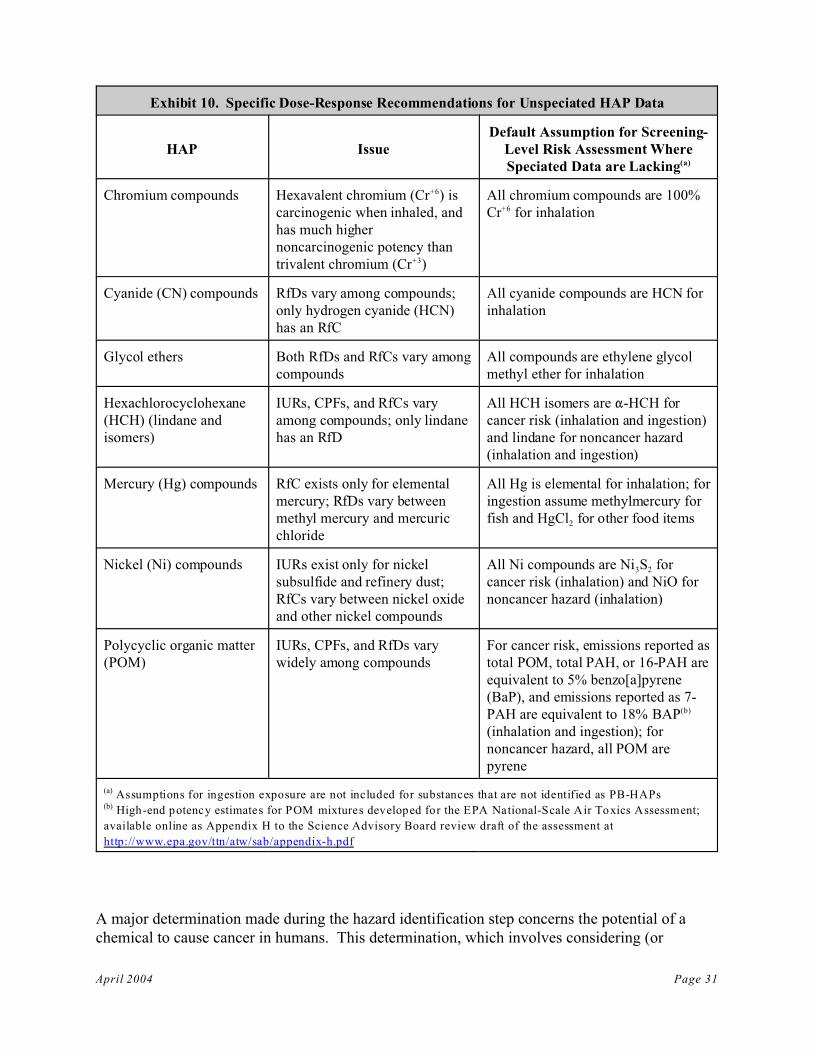
April 2004 Page 31
Exhibit 10. Specific Dose-Response Recommendations for Unspeciated HAP Data
HAP IssueDefault Assumption for Screening-
Level Risk Assessment WhereSpeciated Data are Lacking(a)
Chromium compounds Hexavalent chromium (Cr+6) iscarcinogenic when inhaled, andhas much highernoncarcinogenic potency thantrivalent chromium (Cr+3)
All chromium compounds are 100%Cr+6 for inhalation
Cyanide (CN) compounds RfDs vary among compounds;only hydrogen cyanide (HCN)has an RfC
All cyanide compounds are HCN forinhalation
Glycol ethers Both RfDs and RfCs vary amongcompounds
All compounds are ethylene glycolmethyl ether for inhalation
Hexachlorocyclohexane(HCH) (lindane andisomers)
IURs, CPFs, and RfCs varyamong compounds; only lindanehas an RfD
All HCH isomers are "-HCH forcancer risk (inhalation and ingestion)and lindane for noncancer hazard(inhalation and ingestion)
Mercury (Hg) compounds RfC exists only for elementalmercury; RfDs vary betweenmethyl mercury and mercuricchloride
All Hg is elemental for inhalation; foringestion assume methylmercury forfish and HgCl2 for other food items
Nickel (Ni) compounds IURs exist only for nickelsubsulfide and refinery dust;RfCs vary between nickel oxideand other nickel compounds
All Ni compounds are Ni3S2 forcancer risk (inhalation) and NiO fornoncancer hazard (inhalation)
Polycyclic organic matter(POM)
IURs, CPFs, and RfDs varywidely among compounds
For cancer risk, emissions reported astotal POM, total PAH, or 16-PAH areequivalent to 5% benzo[a]pyrene(BaP), and emissions reported as 7-PAH are equivalent to 18% BAP(b)
(inhalation and ingestion); fornoncancer hazard, all POM arepyrene
(a) Assumptions for ingestion exposure are not included for substances that are not identified as PB-HAPs(b) High-end potency estimates for POM mixtures developed for the EPA National-Scale Air Toxics Assessment;
available online as Appendix H to the Science Advisory Board review draft of the assessment at
http://www.epa.gov/ttn/atw/sab/appendix-h.pdf
A major determination made during the hazard identification step concerns the potential of achemical to cause cancer in humans. This determination, which involves considering (or
April 2004 Page 32
weighing) all the available evidence, is called the weight of evidence (WOE) determination. This determination is complicated by possible inadequacies of the published studies as well asdifferences in body processes between people and laboratory animals. EPA’s Guidelines forCarcinogen Risk Assessment(11) guide scientists in interpreting available studies to assess thepotential human carcinogenicity of environmental pollutants. When compared with EPA’soriginal 1986 guidelines, the 1999 interim Guidelines recommend a more comprehensiveevaluation of the evidence with regard to a chemical’s potential mode of action, and a morecomplete description of the context of a chemical’s carcinogenic potential (e.g., “likelycarcinogenic by inhalation and not likely carcinogenic by oral exposure”). The WOEdetermination now includes one of five descriptors and is accompanied by additional text thatmore completely summarizes EPA’s interpretation of the evidence. The narrative statementsconsider the quality and adequacy of data and the consistency of responses induced by the agentin question (see Volume 1, Chapter 12).
Dose-response values (e.g., IURs, RfCs) are used in risk assessment to estimate the potential foradverse impacts resulting from exposure to a given concentration of a HAP. Identifying criticalhuman health endpoints (cancer vs. non-cancer) and target organs is crucial for structuring therisk assessment, including determining what exposure pathways and routes are of potentialconcern, and how to sum the risks from exposure to multiple HAPs. Volume 1 of this seriesprovides more details of this process. For each HAP included in a risk assessment, the riskassessor identifies the critical human health endpoints and target organs to ensure that cumulativerisk across all HAPs is estimated in a manner consistent with risk assessment principles duringthe risk characterization step. The discussion of health effects criteria used by EPA in the NATA1996 National-Scale Assessment(12) provides one example of how to identify dose-responsevalues for a specific assessment when data from a variety of sources are available.
As noted in Volume 1 (Chapter 12), the derivation of dose-response values includes uncertaintyfactors and confidence levels, which vary widely among chemicals. This information should beincluded in the risk assessment and discussed in the risk characterization.
• Chronic effects. EPA/OAQPS has developed a set of recommended chronic human healthdose-response values for many HAPs. This information includes the type of hazard (e.g.,cancer, non-cancer) and the applicable dose-response values for each HAP (e.g., RfCs,IURs). It is presented in Appendix C of Volume 1. The most up-to-date list of defaultscreening level dose-response values recommended by EPA for the 188 HAPs is provided athttp://www.epa.gov/ttn/atw/toxsource/summary.html. This dose-response information isgenerally appropriate to use in any tier of a risk assessment. However, OAQPS recognizesthat other independently-reviewed dose-response values may also be appropriate to use in tier2 and 3 assessments. These values should be consistent with EPA risk assessment guidelinesand agreed upon in advance with the appropriate regulatory authority for assessments thathave regulatory implications. Descriptive information on the type of health hazardsassociated with each HAP (e.g., cancer, noncancer) may be found athttp://www.epa.gov/ttn/atw/hapindex.html.
– The Inhalation Unit Risk (IUR) is used to estimate inhalation cancer risk. The IUR isdefined as the upper-bound excess lifetime cancer risk estimated to result fromcontinuous exposure to an agent via inhalation per 1 µg/m3 over a lifetime. The
April 2004 Page 33
interpretation of unit risk would be as follows: if the IUR = 1.5 × 10⁻⁶ per µg/m3, then notmore than1.5 excess tumors may be expected to develop per 1,000,000 people if exposedcontinuously for a lifetime to 1 µg of the chemical per cubic meter of air inhaled. Thenumber of expected tumors may be less; it may even be none.
– The Reference Concentration (RfC) is used to estimate the potential for adverse effectsdue to chronic inhalation exposures. The RfC is defined as an estimate (with uncertaintyspanning perhaps an order of magnitude) of a continuous inhalation exposure to thehuman population (including sensitive subpopulations) that is likely to be without anappreciable risk of deleterious effects during a lifetime. RfCs are normally expressed asmilligrams per cubic meter (mg/m3). This is generally used in EPA’s health effectsassessments for effects other than cancer.
• Acute effects. Volume 1 of this reference library (Chapter 12) identifies and describes avariety of short term, acute exposure values that may be used to assess the potential foradverse impacts due to acute inhalation exposures. As noted in Volume 1, acute criteria aredeveloped to match specific time scales of exposure (available sources use different exposuretimes) and desired effect levels (e.g., no-effect or mild reversible effects). One-hour acuteexposure times are commonly used for facility/source-specific risk assessments. EPAsuggests comparing estimated 1-hour exposures to a range of acute dose-response valuesfrom the sources noted below. Note that these values have been developed for differentpurposes (e.g., some may represent mild effect levels, and some may consider economics ortechnical feasibility) and should be used with caution.
– Acute Reference Exposure (ARE) values. The ARE is an informed estimate of thehighest inhalation exposure (concentration and duration) that is not likely to causeadverse effects in a human population, including sensitive subgroups, exposed to thatscenario, even on an intermittent basis.(13) For these purposes, acute exposures are singlecontinuous exposures lasting 24 hours or less; AREs may be derived for any duration ofinterest within that period. “Intermittent” implies sufficient time between exposures suchthat one exposure has no effect on the health outcome produced by the next exposure. EPA is in the process of finalizing the methodology for development of AREs.
– 1-hour Acute Exposure Guideline Levels (AEGL-1 values). The AEGL-1 is theairborne concentration, parts per million (ppm) or mg/m3 of a substance above which it ispredicted that the general population, including “susceptible” but excluding“hypersusceptible” individuals, could experience notable discomfort, irritation, or certainasymptomatic non-sensory effects. However, the effects are not disabling and aretransient and reversible upon cessation of exposure. These values are not intended forevaluating the acute effects associated with frequent exposures; however, the use here isin comparison to the highest 1-hour exposure concentration. AEGL-1 values andsupplementary information are developed by a National Advisory Committee, for use byfederal, state, and local agencies and organizations in the private sector concerned withemergency planning, prevention, and response.
– Acute Reference Exposure Levels (REL values). The REL is a chemical-specific acuteexposure level estimate for noncancer effects (with an uncertainty spanning an order of

April 2004 Page 34
magnitude) that is not likely to cause adverse effects in a human population after acuteexposure to inhaled chemicals other than criteria air pollutants. Note that some acuteRELs have different averaging periods other than one hour (e.g., 4, 5, and 6 hours). RELsare developed by the California Office of Environmental Health Hazard Assessment(OEHHA), and are available with supporting information athttp://www.oehha.ca.gov/air/acute_rels/index.html.
– Emergency Response Planning Guidelines (ERPG-1 values). The ERPG-1 is themaximum concentration in air below which it is believed that nearly all individuals couldbe exposed for up to one hour without experiencing other than mild transient adversehealth effects or perceiving a clearly defined objectionable odor. These values are notintended for evaluating the acute effects associated with frequent exposures; however, theuse here is in comparison to the highest 1-hour exposure concentration. ERPG-1 valuesare developed by the American Industrial Hygiene Association (AIHA) and are availableon-line via the US Department of Energy at http://www.bnl.gov/scapa/scapawl.htm.
– Acute Minimum Risk Levels (MRL values). The MRL is an estimate of humanexposure to a substance that is likely to be without an appreciable risk of adverse effects(other than cancer) over a specified duration of exposure, and can be derived for acuteexposures by the inhalation and oral routes. Unlike the one-hour focus of most of theother values listed here, acute MRLs are derived for exposures of 1 to 14 days duration. Acute MRLs are developed by the US Agency for Toxic Substances and Disease Registry(ATSDR), and are available at http://www.atsdr.cdc.gov/mrls.html.
– 1/10 Levels Imminently Dangerous to Life and Health (IDLH/10 Values). IDLHvalues are exactly as described, and are intended to trigger immediate evacuation of workareas. However, levels one-tenth of the IDLH tend to be generally similar to mild effectlevels such as AEGL-1s or ERG-1s, and are included with EPA/OAQPS’s acute valuestable on this basis. The IDLH/10 has been used commonly as the level of concern(superceded by ERPG and AEGL values, as available) in the Agency’s emergencyplanning programs pursuant to the Emergency Planning and Community Right-to-KnowAct (EPCRA) and Section 112(r) of the Clean Air Act. Although the use of IDLH/10values is not ideal, in many cases these values represent the only readily-available acutedose-response value. IDLHs are developed by the National Institute for OccupationalSafety and Health (NIOSH) as part of its mission to study and protect worker health, andare available at http://www.cdc.gov/niosh/idlh/idlh-1.html.
April 2004 Page 35
Derivation of Dose-Response Values
To understand the potential toxicity of a specific chemical, risk assessors must know both the type ofeffect it produces (the hazard) and the level of exposure required to produce that effect (the dose-response relationship). Both hazard and dose-response information are derived from availablehuman epidemiologic data, experimental animal studies, and supporting information such as in vitrolaboratory tests. This information can provide a quantitative estimate of the relationship between dose,the level of exposure, and response, the increased likelihood and/or severity of adverse effects. Dose-response assessment is the process of quantitatively evaluating toxicity information,characterizing the relationship between the dose of the contaminant administered and the incidence ofadverse health effects in the exposed subjects (which may be animal or human) and then, asappropriate, extrapolating these results to human populations. Depending on the type of effect and thechemical, there are two types of dose-response values that traditionally may be derived: predictivecancer risk estimates, such as the inhalation unit risk estimate (IUR), and the reference value, suchas the reference concentration (RfC). Both types of dose-response value may be developed for thesame chemical, as appropriate.
An important aspect of dose-response relationships is whether the available evidence suggests theexistence of a threshold. For many types of toxic responses, there is a threshold dose below whichthere are thought to be no adverse effects from exposure to the chemical. The human body hasdefenses against many toxic agents. Cells in human organs, especially in the liver and kidneys, breakdown many chemicals into less toxic substances that can be eliminated from the body. In this way, thehuman body can withstand some toxic insult (at doses below the threshold) and still remain healthy. Many HAPs are naturally occurring substances to which people routinely receive trace exposures atnon-toxic levels.
Depending on whether a substance causes cancer and whether its dose-response curve is thought tohave a threshold, EPA may use either of two approaches in a dose-response assessment. One approachproduces a predictive estimate (e.g., inhalation cancer risk estimate), and the other produces areference value (e.g., RfC). Historically, the use of a predictive estimate has been limited to cancerassessment. That is, dose-response assessments for cancer have been expressed as predictive cancerrisk estimates based on an assumption that any amount of exposure poses some risk. Assessments ofeffects other than cancer usually have been expressed as reference values at or below which no harm isexpected. Many substances have been assessed both ways: the first for cancer and the second foradverse effects other than cancer. While this use of predictive estimates for cancer and referencevalues for other effects is still the practice for the vast majority of chemicals, EPA now recognizes thatthere are chemicals for which the data support an alternate approach (see Volume 1, Chapter 12).
Epidemiologic and toxicologic data on air toxics typically result from exposure levels that are highrelative to environmental levels, therefore low-dose extrapolation (prediction) is necessary to derivean applicable dose-response value. Low-dose extrapolation requires either information or assumptionsabout the type of dose-response curve likely under low dose situations. Confidence in the toxicitylevels is indicated for noncarcinogens by applying uncertainty and modifying factors and bydiscussion of the confidence level. Confidence for carcinogens is indicated by EPA’s weight ofevidence evaluations. Volume 1, Chapter 12 provides a more detailed discussion of the derivation ofdose-response values.
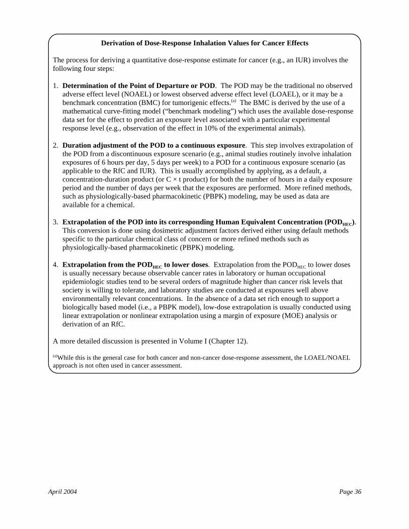
April 2004 Page 36
Derivation of Dose-Response Inhalation Values for Cancer Effects
The process for deriving a quantitative dose-response estimate for cancer (e.g., an IUR) involves thefollowing four steps:
1. Determination of the Point of Departure or POD. The POD may be the traditional no observedadverse effect level (NOAEL) or lowest observed adverse effect level (LOAEL), or it may be abenchmark concentration (BMC) for tumorigenic effects.(a) The BMC is derived by the use of amathematical curve-fitting model (“benchmark modeling”) which uses the available dose-responsedata set for the effect to predict an exposure level associated with a particular experimentalresponse level (e.g., observation of the effect in 10% of the experimental animals).
2. Duration adjustment of the POD to a continuous exposure. This step involves extrapolation ofthe POD from a discontinuous exposure scenario (e.g., animal studies routinely involve inhalationexposures of 6 hours per day, 5 days per week) to a POD for a continuous exposure scenario (asapplicable to the RfC and IUR). This is usually accomplished by applying, as a default, aconcentration-duration product (or C × t product) for both the number of hours in a daily exposureperiod and the number of days per week that the exposures are performed. More refined methods,such as physiologically-based pharmacokinetic (PBPK) modeling, may be used as data areavailable for a chemical.
3. Extrapolation of the POD into its corresponding Human Equivalent Concentration (PODHEC). This conversion is done using dosimetric adjustment factors derived either using default methodsspecific to the particular chemical class of concern or more refined methods such asphysiologically-based pharmacokinetic (PBPK) modeling.
4. Extrapolation from the PODHEC to lower doses. Extrapolation from the PODHEC to lower dosesis usually necessary because observable cancer rates in laboratory or human occupationalepidemiologic studies tend to be several orders of magnitude higher than cancer risk levels thatsociety is willing to tolerate, and laboratory studies are conducted at exposures well aboveenvironmentally relevant concentrations. In the absence of a data set rich enough to support abiologically based model (i.e., a PBPK model), low-dose extrapolation is usually conducted usinglinear extrapolation or nonlinear extrapolation using a margin of exposure (MOE) analysis orderivation of an RfC.
A more detailed discussion is presented in Volume I (Chapter 12).
(a)While this is the general case for both cancer and non-cancer dose-response assessment, the LOAEL/NOAELapproach is not often used in cancer assessment.
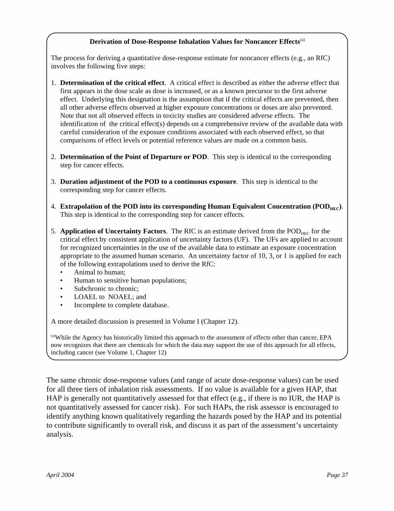
April 2004 Page 37
Derivation of Dose-Response Inhalation Values for Noncancer Effects(a)
The process for deriving a quantitative dose-response estimate for noncancer effects (e.g., an RfC)involves the following five steps:
1. Determination of the critical effect. A critical effect is described as either the adverse effect thatfirst appears in the dose scale as dose is increased, or as a known precursor to the first adverseeffect. Underlying this designation is the assumption that if the critical effects are prevented, thenall other adverse effects observed at higher exposure concentrations or doses are also prevented. Note that not all observed effects in toxicity studies are considered adverse effects. Theidentification of the critical effect(s) depends on a comprehensive review of the available data withcareful consideration of the exposure conditions associated with each observed effect, so thatcomparisons of effect levels or potential reference values are made on a common basis.
2. Determination of the Point of Departure or POD. This step is identical to the correspondingstep for cancer effects.
3. Duration adjustment of the POD to a continuous exposure. This step is identical to thecorresponding step for cancer effects.
4. Extrapolation of the POD into its corresponding Human Equivalent Concentration (PODHEC). This step is identical to the corresponding step for cancer effects.
5. Application of Uncertainty Factors. The RfC is an estimate derived from the PODHEC for thecritical effect by consistent application of uncertainty factors (UF). The UFs are applied to accountfor recognized uncertainties in the use of the available data to estimate an exposure concentrationappropriate to the assumed human scenario. An uncertainty factor of 10, 3, or 1 is applied for eachof the following extrapolations used to derive the RfC:• Animal to human;• Human to sensitive human populations;• Subchronic to chronic;• LOAEL to NOAEL; and• Incomplete to complete database.
A more detailed discussion is presented in Volume I (Chapter 12).
(a)While the Agency has historically limited this approach to the assessment of effects other than cancer, EPAnow recognizes that there are chemicals for which the data may support the use of this approach for all effects,including cancer (see Volume 1, Chapter 12)
The same chronic dose-response values (and range of acute dose-response values) can be usedfor all three tiers of inhalation risk assessments. If no value is available for a given HAP, thatHAP is generally not quantitatively assessed for that effect (e.g., if there is no IUR, the HAP isnot quantitatively assessed for cancer risk). For such HAPs, the risk assessor is encouraged toidentify anything known qualitatively regarding the hazards posed by the HAP and its potentialto contribute significantly to overall risk, and discuss it as part of the assessment’s uncertaintyanalysis.
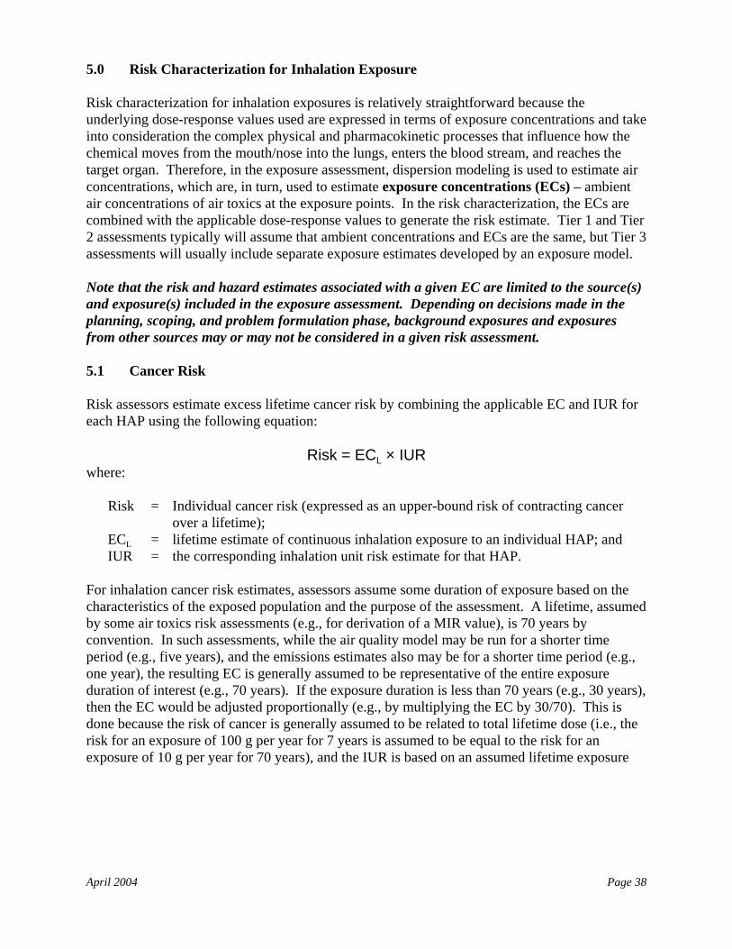
April 2004 Page 38
5.0 Risk Characterization for Inhalation Exposure
Risk characterization for inhalation exposures is relatively straightforward because theunderlying dose-response values used are expressed in terms of exposure concentrations and takeinto consideration the complex physical and pharmacokinetic processes that influence how thechemical moves from the mouth/nose into the lungs, enters the blood stream, and reaches thetarget organ. Therefore, in the exposure assessment, dispersion modeling is used to estimate airconcentrations, which are, in turn, used to estimate exposure concentrations (ECs) – ambientair concentrations of air toxics at the exposure points. In the risk characterization, the ECs arecombined with the applicable dose-response values to generate the risk estimate. Tier 1 and Tier2 assessments typically will assume that ambient concentrations and ECs are the same, but Tier 3assessments will usually include separate exposure estimates developed by an exposure model.
Note that the risk and hazard estimates associated with a given EC are limited to the source(s)and exposure(s) included in the exposure assessment. Depending on decisions made in theplanning, scoping, and problem formulation phase, background exposures and exposuresfrom other sources may or may not be considered in a given risk assessment.
5.1 Cancer Risk
Risk assessors estimate excess lifetime cancer risk by combining the applicable EC and IUR foreach HAP using the following equation:
Risk = ECL × IURwhere:
Risk = Individual cancer risk (expressed as an upper-bound risk of contracting cancerover a lifetime);
ECL = lifetime estimate of continuous inhalation exposure to an individual HAP; andIUR = the corresponding inhalation unit risk estimate for that HAP.
For inhalation cancer risk estimates, assessors assume some duration of exposure based on thecharacteristics of the exposed population and the purpose of the assessment. A lifetime, assumedby some air toxics risk assessments (e.g., for derivation of a MIR value), is 70 years byconvention. In such assessments, while the air quality model may be run for a shorter timeperiod (e.g., five years), and the emissions estimates also may be for a shorter time period (e.g.,one year), the resulting EC is generally assumed to be representative of the entire exposureduration of interest (e.g., 70 years). If the exposure duration is less than 70 years (e.g., 30 years),then the EC would be adjusted proportionally (e.g., by multiplying the EC by 30/70). This isdone because the risk of cancer is generally assumed to be related to total lifetime dose (i.e., therisk for an exposure of 100 g per year for 7 years is assumed to be equal to the risk for anexposure of 10 g per year for 70 years), and the IUR is based on an assumed lifetime exposure
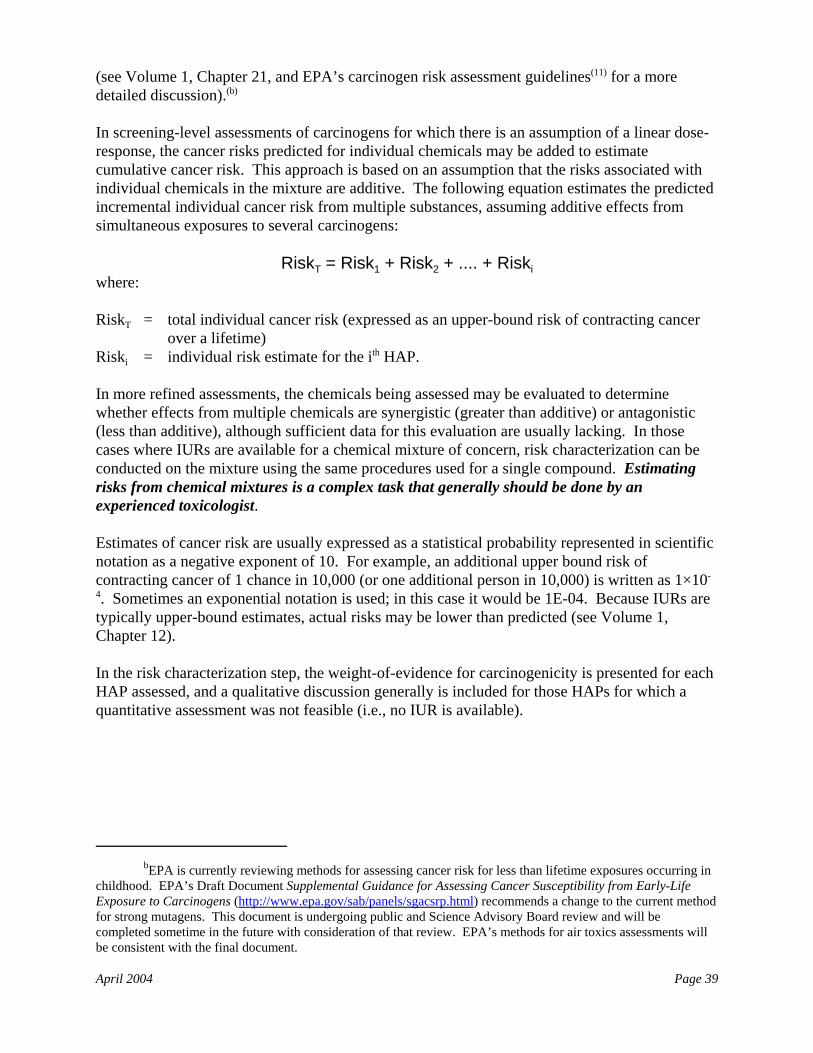
bEPA is currently reviewing methods for assessing cancer risk for less than lifetime exposures occurring inchildhood. EPA’s Draft Document Supplemental Guidance for Assessing Cancer Susceptibility from Early-LifeExposure to Carcinogens (http://www.epa.gov/sab/panels/sgacsrp.html) recommends a change to the current methodfor strong mutagens. This document is undergoing public and Science Advisory Board review and will becompleted sometime in the future with consideration of that review. EPA’s methods for air toxics assessments willbe consistent with the final document.
April 2004 Page 39
(see Volume 1, Chapter 21, and EPA’s carcinogen risk assessment guidelines(11) for a moredetailed discussion).(b)
In screening-level assessments of carcinogens for which there is an assumption of a linear dose-response, the cancer risks predicted for individual chemicals may be added to estimatecumulative cancer risk. This approach is based on an assumption that the risks associated withindividual chemicals in the mixture are additive. The following equation estimates the predictedincremental individual cancer risk from multiple substances, assuming additive effects fromsimultaneous exposures to several carcinogens:
RiskT = Risk1 + Risk2 + .... + Riskiwhere:
RiskT = total individual cancer risk (expressed as an upper-bound risk of contracting cancerover a lifetime)
Riski = individual risk estimate for the ith HAP.
In more refined assessments, the chemicals being assessed may be evaluated to determinewhether effects from multiple chemicals are synergistic (greater than additive) or antagonistic(less than additive), although sufficient data for this evaluation are usually lacking. In thosecases where IURs are available for a chemical mixture of concern, risk characterization can beconducted on the mixture using the same procedures used for a single compound. Estimatingrisks from chemical mixtures is a complex task that generally should be done by anexperienced toxicologist.
Estimates of cancer risk are usually expressed as a statistical probability represented in scientificnotation as a negative exponent of 10. For example, an additional upper bound risk ofcontracting cancer of 1 chance in 10,000 (or one additional person in 10,000) is written as 1×10-
4. Sometimes an exponential notation is used; in this case it would be 1E-04. Because IURs aretypically upper-bound estimates, actual risks may be lower than predicted (see Volume 1,Chapter 12).
In the risk characterization step, the weight-of-evidence for carcinogenicity is presented for eachHAP assessed, and a qualitative discussion generally is included for those HAPs for which aquantitative assessment was not feasible (i.e., no IUR is available).
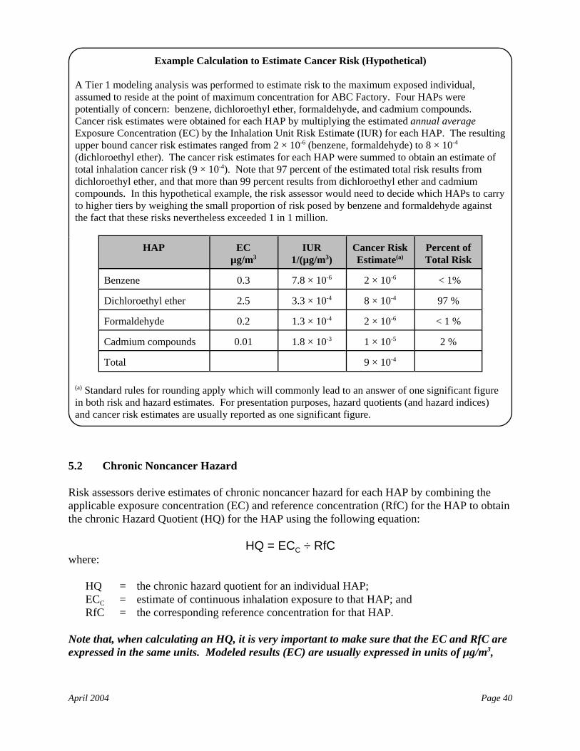
April 2004 Page 40
Example Calculation to Estimate Cancer Risk (Hypothetical)
A Tier 1 modeling analysis was performed to estimate risk to the maximum exposed individual,assumed to reside at the point of maximum concentration for ABC Factory. Four HAPs werepotentially of concern: benzene, dichloroethyl ether, formaldehyde, and cadmium compounds. Cancer risk estimates were obtained for each HAP by multiplying the estimated annual averageExposure Concentration (EC) by the Inhalation Unit Risk Estimate (IUR) for each HAP. The resultingupper bound cancer risk estimates ranged from 2 × 10⁻⁶ (benzene, formaldehyde) to 8 × 10⁻⁴
(dichloroethyl ether). The cancer risk estimates for each HAP were summed to obtain an estimate oftotal inhalation cancer risk (9 × 10⁻⁴). Note that 97 percent of the estimated total risk results fromdichloroethyl ether, and that more than 99 percent results from dichloroethyl ether and cadmiumcompounds. In this hypothetical example, the risk assessor would need to decide which HAPs to carryto higher tiers by weighing the small proportion of risk posed by benzene and formaldehyde againstthe fact that these risks nevertheless exceeded 1 in 1 million.
HAP ECµg/m3
IUR1/(µg/m3)
Cancer RiskEstimate(a)
Percent ofTotal Risk
Benzene 0.3 7.8 × 10⁻⁶ 2 × 10⁻⁶ < 1%
Dichloroethyl ether 2.5 3.3 × 10⁻⁴ 8 × 10⁻⁴ 97 %
Formaldehyde 0.2 1.3 × 10⁻⁴ 2 × 10⁻⁶ < 1 %
Cadmium compounds 0.01 1.8 × 10⁻³ 1 × 10⁻⁵ 2 %
Total 9 × 10⁻⁴
(a) Standard rules for rounding apply which will commonly lead to an answer of one significant figurein both risk and hazard estimates. For presentation purposes, hazard quotients (and hazard indices)and cancer risk estimates are usually reported as one significant figure.
5.2 Chronic Noncancer Hazard
Risk assessors derive estimates of chronic noncancer hazard for each HAP by combining theapplicable exposure concentration (EC) and reference concentration (RfC) for the HAP to obtainthe chronic Hazard Quotient (HQ) for the HAP using the following equation:
HQ = ECC ÷ RfCwhere:
HQ = the chronic hazard quotient for an individual HAP;ECC = estimate of continuous inhalation exposure to that HAP; andRfC = the corresponding reference concentration for that HAP.
Note that, when calculating an HQ, it is very important to make sure that the EC and RfC areexpressed in the same units. Modeled results (EC) are usually expressed in units of µg/m3,
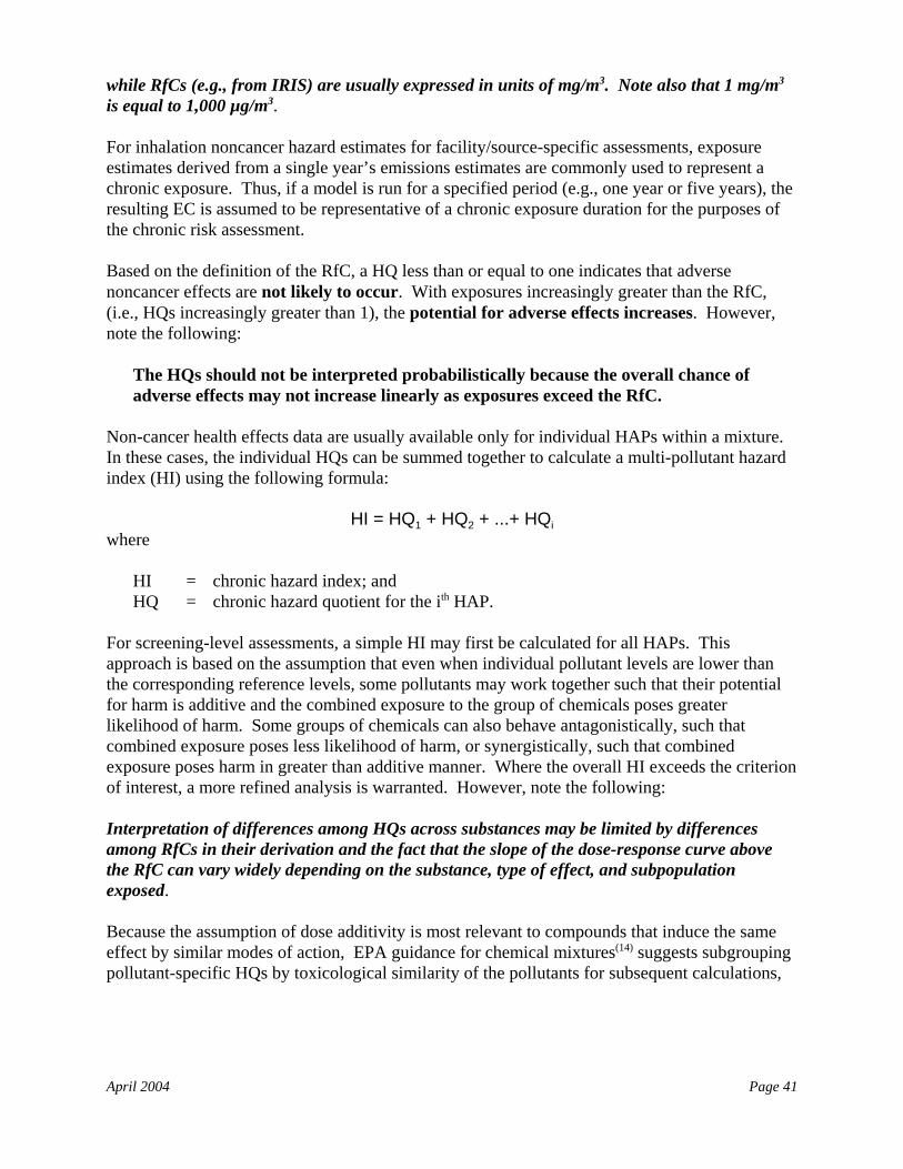
April 2004 Page 41
while RfCs (e.g., from IRIS) are usually expressed in units of mg/m3. Note also that 1 mg/m3
is equal to 1,000 µg/m3.
For inhalation noncancer hazard estimates for facility/source-specific assessments, exposureestimates derived from a single year’s emissions estimates are commonly used to represent achronic exposure. Thus, if a model is run for a specified period (e.g., one year or five years), theresulting EC is assumed to be representative of a chronic exposure duration for the purposes ofthe chronic risk assessment.
Based on the definition of the RfC, a HQ less than or equal to one indicates that adversenoncancer effects are not likely to occur. With exposures increasingly greater than the RfC,(i.e., HQs increasingly greater than 1), the potential for adverse effects increases. However,note the following:
The HQs should not be interpreted probabilistically because the overall chance ofadverse effects may not increase linearly as exposures exceed the RfC.
Non-cancer health effects data are usually available only for individual HAPs within a mixture. In these cases, the individual HQs can be summed together to calculate a multi-pollutant hazardindex (HI) using the following formula:
HI = HQ1 + HQ2 + ...+ HQiwhere
HI = chronic hazard index; andHQ = chronic hazard quotient for the ith HAP.
For screening-level assessments, a simple HI may first be calculated for all HAPs. Thisapproach is based on the assumption that even when individual pollutant levels are lower thanthe corresponding reference levels, some pollutants may work together such that their potentialfor harm is additive and the combined exposure to the group of chemicals poses greaterlikelihood of harm. Some groups of chemicals can also behave antagonistically, such thatcombined exposure poses less likelihood of harm, or synergistically, such that combinedexposure poses harm in greater than additive manner. Where the overall HI exceeds the criterionof interest, a more refined analysis is warranted. However, note the following:
Interpretation of differences among HQs across substances may be limited by differencesamong RfCs in their derivation and the fact that the slope of the dose-response curve abovethe RfC can vary widely depending on the substance, type of effect, and subpopulationexposed.
Because the assumption of dose additivity is most relevant to compounds that induce the sameeffect by similar modes of action, EPA guidance for chemical mixtures(14) suggests subgroupingpollutant-specific HQs by toxicological similarity of the pollutants for subsequent calculations,
cThe all-HAP HI generally is only used in screening-level (Tier 1) analyses to identify situations where therisk assessor is confident that the estimate of hazard is unlikely to be greater than the risk management decisioncriterion (e.g., a HI greater than 1). The all-HAP HI often is not used in more refined analyses.
April 2004 Page 42
Example Calculation to Estimate Chronic Noncancer Hazard (Hypothetical)
A Tier 1 modeling analysis was performed to estimate chronic noncancer hazard to the maximumexposed individual, assumed to reside at the point of maximum concentration for ABC Factory. FourHAPs were potentially of concern: benzene, dichloroethyl ether, formaldehyde, and cadmiumcompounds. Noncancer hazard estimates were obtained for each HAP by dividing the estimatedExposure Concentration (EC) by the Inhalation Reference Concentration (RfC) for each HAP (notethat the EC is expressed in units of mg/m3 for this analysis). The resulting Hazard quotient (HQ)estimates ranged from 1 × 10⁻³ (formaldehyde) to 1 (cadmium compounds). Note that no RfC wasavailable for dichloroethyl ether. The HQs for each HAP were summed to obtain an estimate of theHazard Index (HI) of 1. Note that cadmium compounds account for 95 percent of the HI, suggestingthat the other HAPs may not need further consideration (although this determination should be madein consideration of all relevant information, including uncertainties such as confidence in the exposureconcentration and uncertainty factors used to derive each RfC).
HAP ECmg/m3
RfC(mg/m3)
HQ(b) Percent ofHI
Benzene 6 × 10⁻⁴ 6 × 10⁻² 1 × 10⁻² 1 %
Dichloroethyl ether(a) 5 × 10⁻³ --- --- ---
Formaldehyde 4 × 10⁻⁴ 9.8 × 10⁻³ 1 × 10⁻³ 4 %
Cadmium compounds 2 × 10⁻⁵ 2 × 10⁻⁵ 1 95 %
Hazard Index (HI) 1
(a) note that the absence of an RfC value means that we cannot quantitatively assess a HAP.(b) Standard rules for rounding apply which will commonly lead to an answer of one significant figure in both riskand hazard estimates. For presentation purposes, hazard quotients (and hazard indices) and cancer risk estimatesare usually reported as one significant figure.
that is, to calculate a target-organ-specific-hazard index (TOSHI) for each subgrouping ofpollutants. This allows for a more refined estimate of overall hazard.(c)
Although the HI approach encompassing all chemicals in a mixture is commonly used for ascreening-level study, it is important to note that application of the HI equation to compoundsthat may produce different effects, or that act by different mechanisms, could overestimate thepotential for effects. Consequently, in a refined assessment, risk assessors commonly calculate aseparate HI for each noncancer endpoint of concern those HAPs with toxicological similarity. Descriptive information on the type of noncancer health hazards associated with each HAP maybe found at http://www.epa.gov/ttn/atw/hapindex.html. Note that assessing hazards fromchemical mixtures (e.g., through calculation of a TOSHI) is a complex task that generallyshould be done by an experienced toxicologist.
April 2004 Page 43
A qualitative discussion generally is included in the risk characterization for those HAPs forwhich a quantitative assessment was not feasible (i.e., no RfC is available).
5.3 Acute Noncancer Hazard
Risk assessors can derive estimates of acute noncancer hazard for each HAP by combining theapplicable short-term exposure concentration (EC) and acute dose-response value (AV) for theHAP to obtain the acute Hazard Quotient (HQ) for the HAP using the following equation:
HQA = ECST ÷ AVwhere:
HQA = the acute hazard quotient for an individual HAP;ECST = estimate of short-term inhalation exposure to that HAP; andAV = the corresponding acute dose-response value for that HAP.
Note that ambient air concentrations are calculated for an exposure duration compatible with theacute dose-response value used.
Acute noncancer health effects data are usually available only for individual HAPs within amixture. In these cases, it may be possible to combine the individual acute HQs to calculate amulti-pollutant acute hazard index (HI) using the following formula:
HIA = HQA1 + HQA2 + ...+ HQAiwhere
HIA = acute hazard index; andHQAi = acute hazard quotient for the ith HAP.
Although this appears similar to the process for combining chronic HQs, the summing of acuteHQs is complicated by several issues that do not pertain to chronic HQs. First, acute dose-response values have been developed for purposes that vary more widely than chronic values. Some sources of acute values define exposures at which adverse effects actually occur, whileother sources develop only no-effect acute values. Second, some acute values are expressed asconcentration-time matrices, while others are expressed as single concentrations for a setexposure duration. Third, some acute values may specifically consider multiple exposures,whereas others consider exposure as a one-time event. Fourth, some sources of acute values areintended to regulate workplace exposures, assuming a population of healthy workers (i.e.,without children, seniors, or other sensitive individuals). Such occupational values may alsoconsider cost and feasibility, factors that EPA considers the province of the risk manager ratherthan the risk assessor.
Given these differences among acute values with regard to their purposes, and the different typesof acute exposure characterization that may be performed, the acute HI analysis is mostinformative when limited to acute values from the same source, the same level of effects, and thesame duration. Analyses that mix sources, effects levels, and durations are likely to bemisleading.
April 2004 Page 44
Risk assessors commonly evaluate acute noncancer hazard using a variety of different acutevalues from different sources, and discuss the resulting hazard estimates considering the purposefor which each of value was developed. This kind of evaluation should only be done by anexperienced toxicologist. The significance of these HQs and HIs would need to beconsidered in the context of the purpose of the risk assessment and the characteristics ofthe dose-response values, such as their purpose, averaging time, and health endpoints. EPAis working to provide more comprehensive guidance on what benchmarks to rely upon and plansto develop a relevant acute benchmark methodology.
5.4 Assessment and Presentation of Uncertainty
The risk estimates used in air toxics risk assessments usually are not fully probabilistic estimatesof risk but conditional estimates given a considerable number of assumptions about exposure andtoxicity. Air toxics risk assessments make use of many different kinds of scientific concepts anddata (e.g., exposure, toxicity, epidemiology), all of which are used to characterize the expectedrisk in a particular environmental context. Informed use of reliable scientific information frommany different sources is a central feature of the risk assessment process. Reliable informationmay or may not be available for many aspects of a risk assessment. Scientific uncertainty isinherent in the risk assessment process, and risk managers almost always must make decisionsusing assessments that are not as definitive in all important areas as would be desirable. Riskassessments also incorporate a variety of professional and science policy judgments (e.g., whichmodels to use, where to locate monitors, which toxicity studies to use as the basis of developingdose-response values). Risk managers therefore need to understand the strengths and thelimitations of each assessment, and to communicate this information to all participants and thepublic.(3) A critical part of the risk characterization process, therefore, is an evaluation of theassumptions, limitations, and uncertainties inherent in the risk assessment in order to place therisk estimates in proper perspective.
One of the key purposes of uncertainty analysis is to provide an understanding of where theestimate of exposure, dose, or risk is likely to fall within the range of possible values. At lowertiers of analysis, this often is expressed as a subjective confidence interval within which there isa high probability that the estimate will fall. When a more quantitative understanding isimportant to the risk management decision, a related analysis, termed “sensitivity analysis” or“analysis of uncertainty importance,” is often performed to identify the relative contribution ofthe uncertainty in a given parameter value (e.g., emission rate, ingestion rate) or modelcomponent to the total uncertainty in the exposure or risk estimate.(15) Often this is used either toidentify which parameter values should be varied to provide high-end vs. central-tendency riskestimates, or to identify parameter values where additional data collection (or modeling effort)can increase the confidence in the resulting risk estimate.
There are numerous sources of uncertainties in air toxics risk assessments, and each meritsconsideration. The degree to which these sources of uncertainty need to be quantified, and theamount of uncertainty that is acceptable, varies considerably on a study-specific basis. For ascreening-level (tier 1) analysis, a high degree of uncertainty is often acceptable, provided thatconservative assumptions are used to bias potential error toward protecting human health. Theuse of conservative assumptions is intended to result in a health-protective estimate where therisk assessor is confident that the risk estimate is unlikely to be greater than the point estimate of
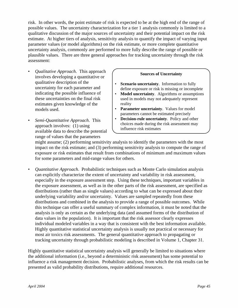
April 2004 Page 45
Sources of Uncertainty
• Scenario uncertainty. Information to fullydefine exposure or risk is missing or incomplete
• Model uncertainty. Algorithms or assumptionsused in models may not adequately representreality
• Parameter uncertainty. Values for modelparameters cannot be estimated precisely
• Decision-rule uncertainty. Policy and otherchoices made during the risk assessment mayinfluence risk estimates
risk. In other words, the point estimate of risk is expected to be at the high end of the range ofpossible values. The uncertainty characterization for a tier 1 analysis commonly is limited to aqualitative discussion of the major sources of uncertainty and their potential impact on the riskestimate. At higher tiers of analysis, sensitivity analysis to quantify the impact of varying inputparameter values (or model algorithms) on the risk estimate, or more complete quantitativeuncertainty analysis, commonly are performed to more fully describe the range of possible orplausible values. There are three general approaches for tracking uncertainty through the riskassessment:
• Qualitative Approach. This approachinvolves developing a quantitative orqualitative description of theuncertainty for each parameter andindicating the possible influence ofthese uncertainties on the final riskestimates given knowledge of themodels used.
• Semi-Quantitative Approach. This
approach involves: (1) usingavailable data to describe the potentialrange of values that the parametersmight assume; (2) performing sensitivity analysis to identify the parameters with the mostimpact on the risk estimate; and (3) performing sensitivity analysis to compute the range ofexposure or risk estimates that result from combinations of minimum and maximum valuesfor some parameters and mid-range values for others.
• Quantitative Approach. Probabilistic techniques such as Monte Carlo simulation analysiscan explicitly characterize the extent of uncertainty and variability in risk assessment,especially in the exposure assessment step. Using these techniques, important variables inthe exposure assessment, as well as in the other parts of the risk assessment, are specified asdistributions (rather than as single values) according to what can be expressed about theirunderlying variability and/or uncertainty. Values are sampled repeatedly from thesedistributions and combined in the analysis to provide a range of possible outcomes. Whilethis technique can offer a useful summary of complex information, it must be noted that theanalysis is only as certain as the underlying data (and assumed forms of the distribution ofdata values in the population). It is important that the risk assessor clearly expressesindividual modeled variables in a way that is consistent with the best information available.Highly quantitative statistical uncertainty analysis is usually not practical or necessary formost air toxics risk assessments. The general quantitative approach to propagating ortracking uncertainty through probabilistic modeling is described in Volume 1, Chapter 31.
Highly quantitative statistical uncertainty analysis will generally be limited to situations wherethe additional information (i.e., beyond a deterministic risk assessment) has some potential toinfluence a risk management decision. Probabilistic analyses, from which the risk results can bepresented as valid probability distributions, require additional resources.
April 2004 Page 46
Additional discussions of uncertainty analysis, including practical approaches to the assessmentand presentation of the principal sources of uncertainty in risk assessments are provided inEPA’s Risk Assessment Guidance for Superfund,(16) guidance documents prepared by EPA andother authors,(4) and in Volume 1 (Chapter 13) of this reference library.
6.0 Tier 1 Inhalation Analysis
6.1 Introduction
This section describes an example approach for performing a Tier 1 inhalation risk assessment. Exhibit 11 provides an overview of this example approach. SCREEN3 or similar models areused for both chronic and acute exposure estimates. Tier 1 analyses incorporate simplifiedassumptions and default values for facility/source-specific modeling inputs that are not readilyavailable, and allow a simple, health-protective risk estimate to be calculated. The resultingexposure estimates are likely to be higher than actual exposures. If the facility/source passes thisscreening analysis, the risk manager can be reasonably confident that the likelihood forsignificant risk is low. This example Tier 1 approach is not intended to prescribe a specificapproach that must be used by EPA or others in a particular risk assessment activity. Inparticular, various modifications to this tiered approach may be both cost-effective andappropriate, such as adding intermediate-level tiers that incorporate some features of thehigher and lower tiers, or conducting iterative, more refined analyses within a given tier. Also, S/L/T agencies may have specific tiered assessment protocols and/or specific modelingguidelines that must be followed. Therefore, consultation with appropriate regulatoryagencies is highly recommended.
Note that this example Tier 1 approach does not incorporate monitoring. While existingmonitoring data may be used as inputs to a Tier 1 analysis, if the Tier 1 results are not sufficientfor the risk management decision, it may be cost-effective to conduct additional analysis (Tier 2or Tier 3) before implementing a new monitoring program.
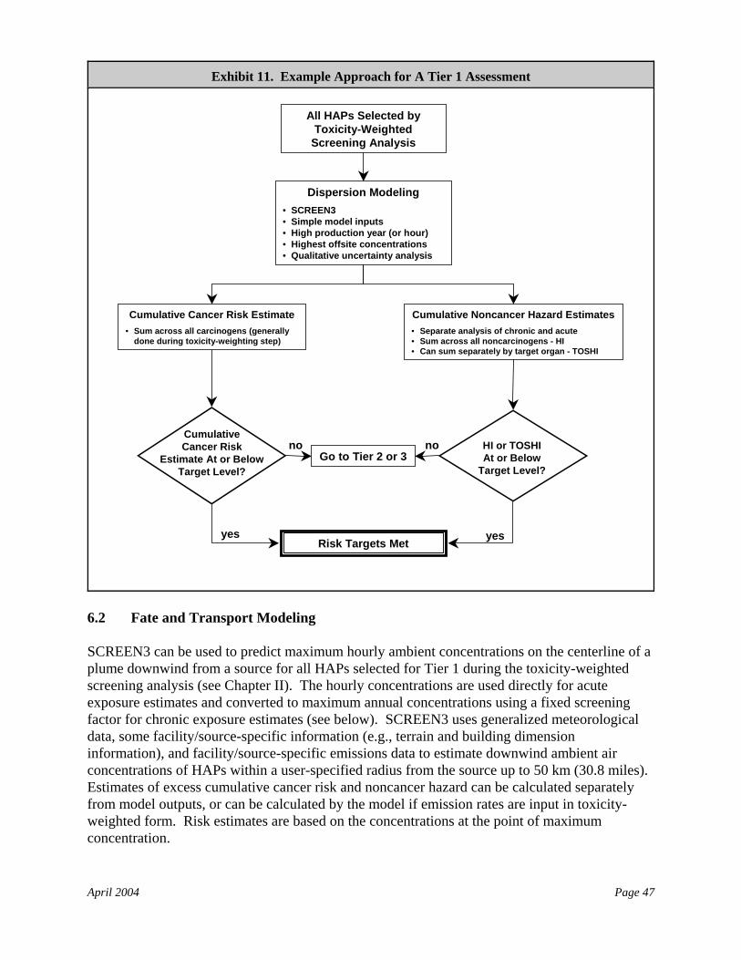
April 2004 Page 47
Dispersion Modeling• SCREEN3• Simple model inputs• High production year (or hour)• Highest offsite concentrations• Qualitative uncertainty analysis
Go to Tier 2 or 3
CumulativeCancer Risk
Estimate At or BelowTarget Level?
Risk Targets Met
no
yes
Cumulative Cancer Risk Estimate• Sum across all carcinogens (generally
done during toxicity-weighting step)
Cumulative Noncancer Hazard Estimates• Separate analysis of chronic and acute• Sum across all noncarcinogens - HI• Can sum separately by target organ - TOSHI
HI or TOSHI At or Below
Target Level?
no
yes
All HAPs Selected by Toxicity-Weighted
Screening Analysis
Exhibit 11. Example Approach for A Tier 1 Assessment
6.2 Fate and Transport Modeling
SCREEN3 can be used to predict maximum hourly ambient concentrations on the centerline of aplume downwind from a source for all HAPs selected for Tier 1 during the toxicity-weightedscreening analysis (see Chapter II). The hourly concentrations are used directly for acuteexposure estimates and converted to maximum annual concentrations using a fixed screeningfactor for chronic exposure estimates (see below). SCREEN3 uses generalized meteorologicaldata, some facility/source-specific information (e.g., terrain and building dimensioninformation), and facility/source-specific emissions data to estimate downwind ambient airconcentrations of HAPs within a user-specified radius from the source up to 50 km (30.8 miles). Estimates of excess cumulative cancer risk and noncancer hazard can be calculated separatelyfrom model outputs, or can be calculated by the model if emission rates are input in toxicity-weighted form. Risk estimates are based on the concentrations at the point of maximumconcentration.
April 2004 Page 48
Where to Find Source Emissions Information
• Facility records or purpose-specific data collection• National Emissions Inventory• State and Federal risk assessment reports• Background Information Documents that support
Maximum Achievable Control Technology Standards(MACT), available from EPA’s MACT docket
• State approved emission permits• Toxics Release Inventory
6.2.1 Model Inputs
Input data for SCREEN3 fall into three categories: (1) emissions data; (2) release parameters(e.g., source type, release temperature, etc.); and (3) building and terrain considerations (e.g.,building downwash and simple or complex terrain). Note that several default parameters formeteorological data are built into SCREEN3. More detailed information is provided in theSCREEN3 User’s Guide.(8) Note that S/L/T agencies may have emissions and other sourceinformation in documents such as state inventories and inspection reports.
• General considerations. Many facilities have multiple emission sources (each with itscharacteristic release height, emissions rate, etc.), and more than one type of emission sourcewithin a single facility. Because SCREEN3 can model a single source per model run, and isnot able to aggregate the results of multiple model runs across different sources, it is mostefficient to combine all sources of each source type (e.g., point, volume) into a single sourcefor Tier 1 analysis (with the receptor assumed to be exposed to the highest concentration atany location). The results for the combined sources of each type are then added together, asif all the releases had occurred at the same point. Because this procedure is health-protectivescreening (e.g., it pessimistically assumes that the highest hourly release rates from allsources will occur simultaneously), it is appropriate for a Tier 1, screening-level analysis.
Exhibit 12 identifies health-protective default values to facilitate Tier 1 analyses. Allfacility/source-specific information needs to be provided in the specific units required bySCREEN3 (and therefore units may need to be converted). As noted earlier, S/L/T agenciesmay have specific modeling guidelines that may differ from the default values presented inExhibit 12.
• Emissions data. In this example approach, the total emissions is the sum of process andfugitive emissions. Process emissions are discrete losses that occur at stacks or process ventsfrom reactors, columns, boilers, and other types of facility equipment. Fugitive emissionsresult from facility equipment leaks, evaporation from waste products, losses from the rawmaterial feed, losses from in-process and final process storage tanks, loading and handlinglosses, and losses from other non-discrete sources.
The risk assessor is encouraged touse the best emissions dataavailable for the facility, includingchemical speciation information. If speciated emissions data are notreadily available, an assumptionthat all HAPs are emitted in themost toxic form commonly is usedin Tier 1 assessments to ensurethat health-protective riskestimates are produced.
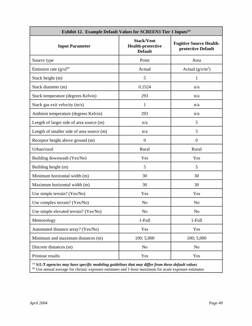
April 2004 Page 49
Exhibit 12. Example Default Values for SCREEN3 Tier 1 Inputs(a)
Input ParameterStack/Vent
Health-protectiveDefault
Fugitive Source Health-protective Default
Source type Point Area
Emission rate (g/s)(b) Actual Actual (g/s/m2)
Stack height (m) 5 1
Stack diameter (m) 0.1524 n/a
Stack temperature (degrees Kelvin) 293 n/a
Stack gas exit velocity (m/s) 1 n/a
Ambient temperature (degrees Kelvin) 293 n/a
Length of larger side of area source (m) n/a 5
Length of smaller side of area source (m) n/a 5
Receptor height above ground (m) 0 0
Urban/rural Rural Rural
Building downwash (Yes/No) Yes Yes
Building height (m) 5 5
Minimum horizontal width (m) 30 30
Maximum horizontal width (m) 30 30
Use simple terrain? (Yes/No) Yes Yes
Use complex terrain? (Yes/No) No No
Use simple elevated terrain? (Yes/No) No No
Meteorology 1-Full 1-Full
Automated distance array? (Yes/No) Yes Yes
Minimum and maximum distances (m) 100; 5,000 100; 5,000
Discrete distances (m) No No
Printout results Yes Yes(a) S/L/T agencies may have specific modeling guidelines that may differ from these default values(b) Use annual average for chronic exposure estimates and 1-hour maximum for acute exposure estimates
April 2004 Page 50
The State of California has determined that the conversion multiplying factors noted above may not bebiased toward over-prediction when the source is not a continuous release. Appendix H of the AirToxics Hot Spots Program Guidance Manual for Preparation of Health Risk Assessments (August2003; http://www.oehha.ca.gov/air/hot_spots/pdf/HRAguidefinal.pdf) presents approaches fordeveloping multiplying factors for (a) non-standard averaging periods with a continuous release; (b)intermittent releases (e.g., releases that occur only from 8 AM to 6 PM); (c) systematic releases (e.g., a“clean-out” release once per day); and (d) random releases.
One common Tier 1 approach is to use emissions data that are representative of maximumannual emissions (e.g., a high-production year). For chronic exposures, the approach usesthe average hourly emissions rate for the high-production year. For acute exposures, theapproach uses the greater of (a) the maximum hourly rate, or (b) ten times the average hourlyrate. The ratio between a longer-term maximum concentration and a 1-hour maximum willdepend upon the duration of the longer averaging time, source characteristics, localclimatology and topography, and the meteorological conditions associated with the 1-hourmaximum. Because of the many ways in which such factors interact, it is not practical tocategorize all situations that will typically result in any specified ratio between thelonger-term and 1-hour maxima. EPA’s Screening Procedures for Estimating the AirQuality Impact of Stationary Sources, Revised(6) identifies ratios for a “general case,” and therisk assessor is given some flexibility to adjust those ratios to represent more closely anyparticular point source application where actual meteorological data are used. Emissions ofmultiple HAPs from a single source can be combined into a single emission using toxicityweighting (see Section 6.2.2 below).
To obtain the estimated maximum concentration for a 3-, 8-, 24-hour or annual averagingtime, multiply the 1-hour maximum concentration by the indicated factor in the table below. The numbers in parentheses are recommended limits to which one may diverge from themultiplying factors representing the general case. For example, if aerodynamic downwash orterrain is a problem at the facility, or if the emission height is very low, it may be necessaryto increase the factors (within the limits specified in parentheses). On the other hand, if thestack is relatively tall and there are no terrain or downwash problems, it may be appropriateto decrease the factors. If the risk assessment involves a regulatory action, the risk assessoris encouraged to discuss these factors with the appropriate regulatory authorities.
Averaging Time Multiplying Factor
3 hours 0.9 (±0.1)
8 hours 0.7 (±0.2)
24 hours 0.4 (±0.2)
Annual 0.08 (±0.02)
Note that some assessments may be based on permit limits (e.g., if their purpose is todetermine if those limits provide adequate protection).
April 2004 Page 51
Building Downwash
Volume 2 of the ISC User’s Guide (Section 1.1.5.3)provides a rule-of-thumb that a building is consideredsufficiently close to a stack to cause wake effectswhen the distance between the stack and the nearestpart of the building is less than or equal to five timesthe lesser of the height or the projected width of thebuilding. This relationship is obviously much morecomplicated with complex building shapes. The ISCUser’s guide is available on EPA’s SCRAM website(http://www.epa.gov/ttn/scram/).
• Release type. SCREEN3 will prompt the user for source-specific characteristics. Pointsources are localized releases from stacks or vents. Flare sources are point sources that havea high release rate (e.g., flames). Area sources are emissions that are spread over an area(e.g., a landfill or lagoon). Volume sources are three-dimensional releases (e.g., fugitiveleaks from an industrial facility). When modeling a facility with multiple sources, assessorstypically model each source separately and sum the resulting maximum concentrations (seebelow).
• Physical release parameters. SCREEN3 will prompt the user for the release parametersappropriate to the type of release. For example, SCREEN3 requires stack height, stackdiameter, stack gas exit velocity, and stack temperature in order to model a point source. When available, it is preferable to use site- or source-specific release parameters. Exampledefault values for point, area, and volume sources (Exhibit 12) can be used whenfacility/source-specific values are not available.
• Meteorological data and buildingand terrain considerations. For thisexample approach, the followinginputs are selected: (1) the “actual”urban/rural dispersion coefficient(based on the site setting); (2) “fullmeteorology” (which considers theeffects of all atmospheric stabilityclasses); (3) building downwash(using either the actual dimensions ofthe largest building in the facility orthe default dimensions in Exhibit 12);and (4) “simple terrain” (elevatedterrain can be entered if appropriatefor the facility/source being evaluated; otherwise, terrain should be assumed flat). Note thatSCREEN3 uses built-in meteorological data (see Volume 1, Chapter 9).
6.2.2 Model Runs
SCREEN3 provides estimates of maximum one-hour ambient concentrations. If multiple modelruns are performed (e.g., separate runs for point sources and area sources), a conservativeapproach is to sum the maximum predicted model results from each run across all sources. Thisapproach assumes that the maximum impact for each source occurs at the same location and thesame hour. These maximum one-hour concentrations can be used to evaluate acute noncancerhazard as described in Section 6.5 below.
SCREEN3 models one HAP for each run of the model. For multiple chemicals, the modeler caninput 1 gram/year as the emission rate and run the model once (or once for each source type). Ambient concentrations for each HAP can then be calculated by multiplying the model results bythe annual emission rate (in tons) for each HAP.
April 2004 Page 52
6.3 Exposure Assessment
Tier 1 assessments will generally assume that the highest ambient concentrations predicted bySCREEN3 are equivalent to exposure concentrations. As noted above, for chronic exposures, theapproach uses the average hourly emissions rate for the high-production year. For acuteexposures, the approach uses the maximum hourly rate, or 10 times the average hourly rate,whichever is greater. If separate model runs were done for some sources (e.g., to separate pointsources from area sources), this example approach sums the maximum exposure concentrationsfrom each model run before characterizing risk. This procedure effectively treats all the releasesas occurring in the same place.
6.4 Risk Characterization
Risk characterization for Tier 1 is limited to estimating inhalation risk at the point of maximumconcentration (calculated separately for cancer risk, chronic noncancer hazard, and acutenoncancer hazard). The exposure concentrations described in Section 6.3 are used to calculaterisk and hazard according to basic equations presented in Section 5 above. Backgroundconcentrations are often not explicitly considered in Tier 1.
• Cancer risk. Excess cumulative cancer risk is calculated by multiplying the maximumannual air concentration by the inhalation IUR for each HAP and summing across all HAPs.
• Chronic noncancer hazard. Chronic cumulative noncancer hazard (the Hazard Index, orHI) is calculated by dividing the maximum annual air concentration by the RfC for each HAPand summing across all HAPs. If the resulting HI exceeds the noncancer target HI level ofregulatory interest, the HI results can be subdivided into a separate Target Organ SpecificHazard Index (TOSHI) for each target organ of concern (see Volume 1, Chapter 13 for amore detailed discussion on how to calculate a TOSHI.).
• Acute noncancer hazard. As discussed in Volume 1, Chapter 13, available acute dose-response values are more diverse than chronic values, because they were developed fordifferent purposes and considering different exposure durations. The most effectivecharacterization of acute risk often is to compare the maximum estimated hourlyconcentrations with a range of acute dose-response values from sources described in Section4 (see an example comparison in Exhibit 13). If the ambient concentration is lower than allthe acute benchmarks, it is generally reasonable to conclude that the potential for significantacute risk is low. If the concentration exceeds some benchmarks but not others, theassessment should describe the benchmark (e.g., is it a no-effect level, or a concentration atwhich mild effects occur?) and discuss the implications of exceeding it.
6.4.1 Reporting Results
A relatively simple summary can be used to report results but should still ensure the results areboth transparent and reproducible. Examples of reports prepared for EPA’s purposes can befound in EPA’s residual risk “test memos;” these may or may not be appropriate examples for thespecific purposes of other risk assessments. The summary generally will include the followinginformation:
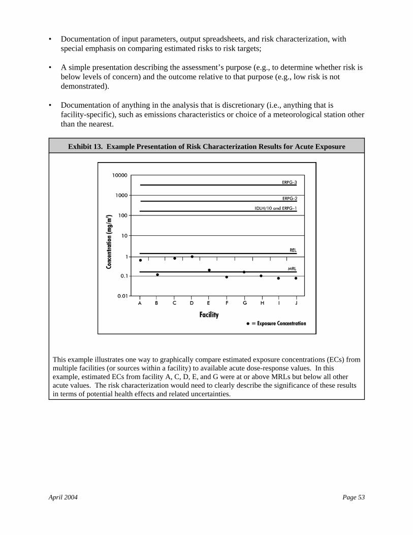
April 2004 Page 53
• Documentation of input parameters, output spreadsheets, and risk characterization, withspecial emphasis on comparing estimated risks to risk targets;
• A simple presentation describing the assessment’s purpose (e.g., to determine whether risk isbelow levels of concern) and the outcome relative to that purpose (e.g., low risk is notdemonstrated).
• Documentation of anything in the analysis that is discretionary (i.e., anything that isfacility-specific), such as emissions characteristics or choice of a meteorological station otherthan the nearest.
Exhibit 13. Example Presentation of Risk Characterization Results for Acute Exposure
This example illustrates one way to graphically compare estimated exposure concentrations (ECs) frommultiple facilities (or sources within a facility) to available acute dose-response values. In thisexample, estimated ECs from facility A, C, D, E, and G were at or above MRLs but below all otheracute values. The risk characterization would need to clearly describe the significance of these resultsin terms of potential health effects and related uncertainties.
April 2004 Page 54
6.4.2 Assessment and Presentation of Uncertainty
Risk managers need to understand the strengths and the limitations of the Tier 1 assessment. Acritical part of the risk characterization process, therefore, is an evaluation of the assumptions,limitations, and uncertainties inherent in the Tier 1 risk assessment in order to place the riskestimates in proper perspective.(3) Tier 1 risk assessments will typically include a quantitative orqualitative description of the uncertainty for each parameter and indicating the possible influenceof these uncertainties on the final risk estimates given knowledge of the models used (i.e., thequalitative approach discussed in Section 5.4 above). The use of conservative assumptions inTier 1 is intended to result in result in a situation where the risk assessor is confident that the riskestimate is unlikely to be greater than the point estimate of risk. In other words, the pointestimate of risk is expected to be at the high end of the range of possible values.
There may be situations where facility/source-specific information is so limited (e.g., emissionsestimates are based on industry-wide values rather than facility/source-specific data; manyfacility/source-specific HAPs are lacking peer-reviewed dose-response values) that the riskassessor may not be confident that the risk estimate is at the high end of possible values. In thesesituations, additional data collection (e.g., to obtain facility/source-specific emissions estimates)and/or a Tier 2 analysis may be appropriate.
6.5 Focusing Tier 2 on the Most Important HAPs/Sources
If cumulative cancer risk and/or noncancer hazard is above the level of concern, a Tier 2 analysismay be needed. This analysis may focus on the particular HAPs and sources that account for ahigh proportion of the estimated risk (at Tier 1) to reduce the Tier 2 analytical effort.
7.0 Tier 2 Inhalation Analysis
7.1 Introduction
This section describes an example approach for performing a Tier 2 inhalation risk assessment. Exhibit 14 provides an overview of this example approach. This example approach uses HEM-3for both chronic and acute exposures, with more facility/source-specific information for HAPs,sources, and potentially exposed populations. Tier 2 analyses may often be limited to thoseHAPs and sources that collectively account for a high proportion of the potential risk or hazardthat was estimated in Tier 1. If the facility/source database permits, risk assessors may be ableto skip Tier 1 entirely and start with Tier 2. For this example Tier 2 approach, HEM-3 providesan estimate of ambient concentrations from all the facility’s sources combined at multipleCensus block internal points, including the Census block with the highest ambient concentration. In this approach to a Tier 2 assessment, these Census block concentrations are used as surrogatesfor exposure concentrations for the people residing there. Note that more complex/advancedexposure modeling is used in the example Tier 3 approach described in Section 7.
The most important differences from Tier 1 are: (1) the exposure surrogate shifts from themaximum offsite ambient concentration to the concentrations within Census blocks (i.e., wherepeople actually reside); (2) individual modeling of release points is performed; and (3) average
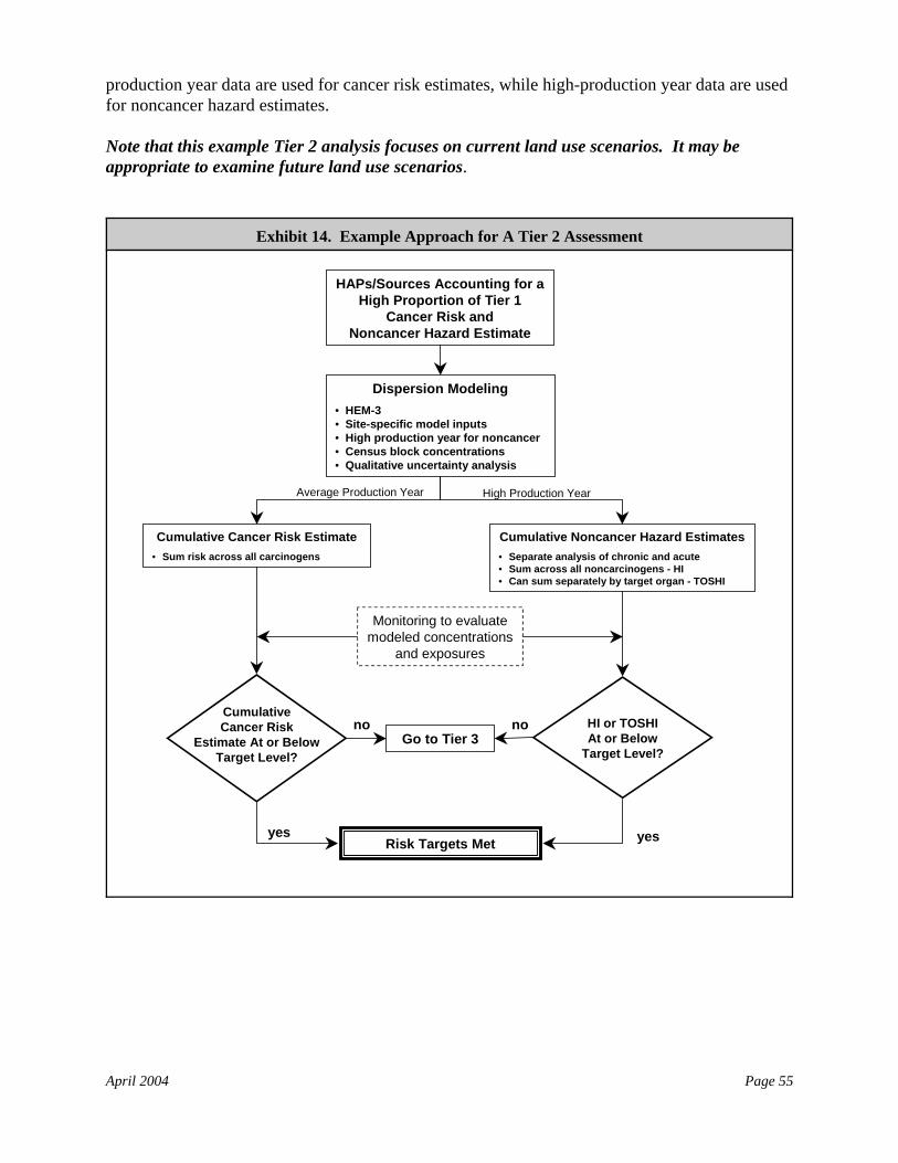
April 2004 Page 55
Dispersion Modeling• HEM-3• Site-specific model inputs• High production year for noncancer• Census block concentrations• Qualitative uncertainty analysis
Go to Tier 3
CumulativeCancer Risk
Estimate At or BelowTarget Level?
Risk Targets Met
no
yes
Cumulative Cancer Risk Estimate• Sum risk across all carcinogens
Cumulative Noncancer Hazard Estimates• Separate analysis of chronic and acute• Sum across all noncarcinogens - HI• Can sum separately by target organ - TOSHI
HI or TOSHIAt or Below
Target Level?
no
yes
HAPs/Sources Accounting for a High Proportion of Tier 1
Cancer Risk andNoncancer Hazard Estimate
Average Production Year High Production Year
Monitoring to evaluate modeled concentrations
and exposures
production year data are used for cancer risk estimates, while high-production year data are usedfor noncancer hazard estimates.
Note that this example Tier 2 analysis focuses on current land use scenarios. It may beappropriate to examine future land use scenarios.
Exhibit 14. Example Approach for A Tier 2 Assessment
April 2004 Page 56
The internal point is only an approximation of where people live. The Census Bureau(a) defines theinternal point as a set of geographic coordinates (latitude and longitude) that is located within aspecified geographic entity. A single point is identified for each entity; for many entities, this pointrepresents the approximate geographic center of that entity. If the shape of the entity causes this pointto be located outside the boundary of the entity or in a water body, it is relocated to land area withinthe entity. The term “centroid” (which is used interchangeably with internal point) is the term morecommonly used by risk assessors when referring to geographic or population-weighted centers. Notethat the internal point established by the Census Bureau is generally set to reflect the geographic centerof the entity in question, regardless of where people actually live in that entity. A populationweighted internal point is a modified point that is considered to better reflect the location of thepeople living in the geographic entity.
(a)U.S. Department of Commerce, U.S. Census Bureau. 2000. Geographic Glossary (Census 2000). Available at: http://www.census.gov/geo/www/tiger/glossry2.pdf
7.2 Fate and Transport Modeling
7.2.1 Model Inputs
Input data for HEM-3 falls into six categories: (1) source location; (2) emissions data; (3)stack/vent parameter data; (4) pollutant specific data (reactivity and dose-response data); (5)meteorological data; and (6) population data. Refinements for Tier 2 are described brieflybelow. More detailed information is provided in the HEM-3 User’s Guide.(7)
• Source location. HEM-3 requires the geographical location (latitude and longitude) of eachsource being simulated. Some of the above sources of geographic information may providecoordinates in Universal Transverse Mercator (UTM) units. The HEM-3 contains a programto convert UTM data into latitude and longitude (e.g., as provided by the use of a GPSreceiver). In many instances there is more than one emission source (each with itscharacteristic release type, height, emissions rate, etc.) within a single facility. HEM-3 canmodel each emission source individually within a single model run. HEM-3 also computesthe total ambient air concentrations resulting from facility emissions by summing theindividual estimates. The geographical location (latitude and longitude) of all sources beingsimulated must be identified. The Tier 2 analysis often will not include a default option toassume that all emission sources are located at single specified latitude and longitude withinthe facility. The model requires that coordinate data be obtained for each emission source inthe analysis, and that each emission source is modeled individually. In other words, thelocation of each source within the facility should be input to HEM-3.
• Emissions data. Depending on the source, the emissions being modeled may be process orfugitive emissions. The risk assessor should use the best site-specific emissions dataavailable, including chemical speciation. As with Tier 1, HEM-3 requires emissions data inthe form of an annual emissions rate (e.g., tons/year). HEM-3 can be used to assess bothchronic and acute exposures. To do this, select “yes” for the “include hourly emissionsvariations” choice, and provide a file of hourly emission rate factors (e.g., 10 times theannual average) appropriate to the type of source for each HAP. Emission rate factors based
April 2004 Page 57
on measured data are preferred, but if measurements are not available, engineering judgmentbased on the nature of the process can be used. For infrequent releases (e.g., less than once amonth), the assessor may assume that the total annual emission rate is released during oneepisode and use engineering judgment to determine the length of the episode.
• Release parameter data. Release parameter data are necessary for dispersion modeling ofthe chemical emissions. Facility/source-specific data generally are preferred for a Tier 2analysis. When these are not available, surrogate data often can be found in the same datasources as the emissions data. HEM-3 release parameter data requirements include:– Stack or area source release height and diameter (meters);– Dimensions of area source (meters);– Stack diameter (meters);– Gas discharge temperature (degrees Kelvin);– Gas emission (exit) velocity (meters/second);– Height of the initial plume (meters); and– Building dimensions (meters, if relevant).
• Atmospheric reactivity and deposition of chemicals. Because the highest inhalationexposures are generally near the source, and little time passes between the release and theexposures, atmospheric reactivity and deposition of fine particles generally do not need to beconsidered in Tier 2.
• Meteorology. HEM-3 uses meteorological data measured both at the surface and in theupper atmosphere in its dispersion calculations. Surface data used by HEM-3 are pre-processed hourly meteorological observations from a user library, or information from auser-specified meteorological station. Upper atmosphere data are twice-daily mixing heightvalues. User-supplied data sets need to be pre-processed by the EPA RAMMET to fit theHEM-3 input format. Surface and upper atmosphere data sets are available from theNational Climate Data Center in Asheville, NC or from the EPA SCRAM website(www.epa.gov/scram001/index.htm).
• Population. In this example of a Tier 2 analysis, modeling is focused on the locations wherepeople actually live. HEM-3 automatically identifies the exposed population using theCensus block internal points already included in the model. These locations are modeleddirectly within a user-specified radius and are interpolated from locations on the polarcoordinate receptor grid for Census blocks outside the radius (Exhibit 15). For Tier 2analyses, all people residing in a Census block are assumed to be continuously exposed to theannual average concentration (and exposed for one hour to the maximum hourlyconcentration) at the interior location within the Census block. Unless otherwise specified,HEM-3 calculates concentrations for each Census block within 50 kilometers of the source’slocation. If a Census block is exposed to emissions from more than one source, HEM-3sums the impacts from each source for each Census block. The model outputs include therisks posed by each HAP at each Census block internal point, the risks from all HAPscombined, and the numbers of people living in Census blocks whose ambient levels fallwithin specified risk ranges.
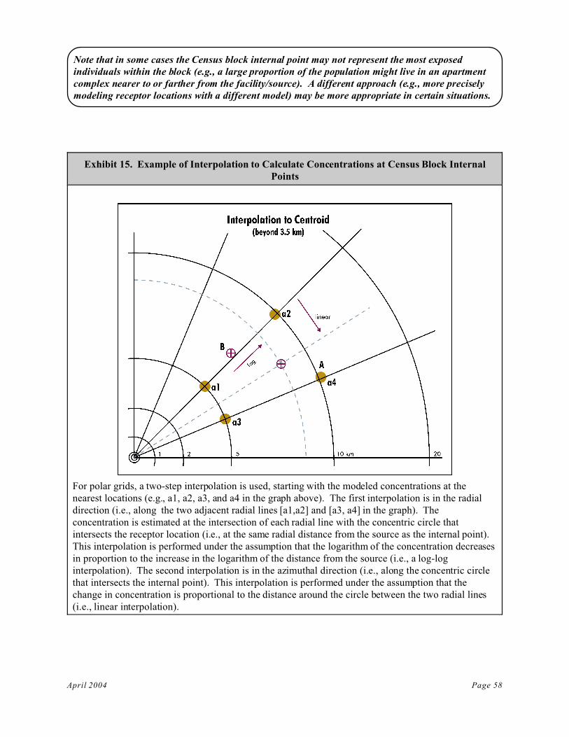
April 2004 Page 58
Note that in some cases the Census block internal point may not represent the most exposedindividuals within the block (e.g., a large proportion of the population might live in an apartmentcomplex nearer to or farther from the facility/source). A different approach (e.g., more preciselymodeling receptor locations with a different model) may be more appropriate in certain situations.
Exhibit 15. Example of Interpolation to Calculate Concentrations at Census Block InternalPoints
For polar grids, a two-step interpolation is used, starting with the modeled concentrations at thenearest locations (e.g., a1, a2, a3, and a4 in the graph above). The first interpolation is in the radialdirection (i.e., along the two adjacent radial lines [a1,a2] and [a3, a4] in the graph). Theconcentration is estimated at the intersection of each radial line with the concentric circle thatintersects the receptor location (i.e., at the same radial distance from the source as the internal point). This interpolation is performed under the assumption that the logarithm of the concentration decreasesin proportion to the increase in the logarithm of the distance from the source (i.e., a log-loginterpolation). The second interpolation is in the azimuthal direction (i.e., along the concentric circlethat intersects the internal point). This interpolation is performed under the assumption that thechange in concentration is proportional to the distance around the circle between the two radial lines(i.e., linear interpolation).
April 2004 Page 59
7.2.2 Model Runs
The following input values can be used to set up HEM-3 model runs for a Tier 2 analysis:
• On screen 1, select “inhalation,” “yes” to both annual and acute concentrations, “1-hour” forthe length of acute exposure, and “rural” for the dispersion environment (unless thefacility/source is located in a densely-populated area).
• Provide the names of the emissions file and the emissions location file, which should be inthe correct spreadsheet format (HEM-3 provides format guidelines).
• Select “no” for the deposition and depletion choices.
• Select “yes” for the terrain elevation choice if the facility/source is located in an area withsubstantial elevation changes; otherwise select “no” for flat topography.
• Select “no” to providing alternate IURs and RfCs.
• Select dimensions of the area to be modeled that are appropriate to the facility. Themaximum radius is 50 kilometers, but for most facilities a radius of 30 kilometers willcapture virtually all important exposures. Select 0 as the minimum radius.
• Select the “distance within which blocks are modeled individually” to capture the Censusblocks with the highest concentrations.
• Choose the appropriate HEM-3 meteorological data file, or provide a facility/source-specific,pre-processed file. Sources of meteorological data are provided in Volume 1, Appendix G.
7.3 Exposure Assessment
The Tier 2 assessment approach described here uses predicted ambient concentrations assurrogates for exposure concentrations. HEM-3 provides estimates of annual averageconcentrations within Census blocks and combines them with chronic dose-response values forcancer and noncancer effects to estimate risk.
7.3.1 Chronic Exposures
HEM-3 provides ambient concentrations for the Census block with the highest annual averagelevels, by individual HAP and emission point. HEM-3 also calculates the upper-bound lifetimecancer risk and noncancer HQs associated with continuous exposure to those ambientconcentrations, and it sums cancer risk across all HAPs and noncancer HQs by target organ. These results can be presented in summary tables (e.g., Exhibits 16 to 19, below).
April 2004 Page 60
7.3.2 Acute Exposures
HEM-3 also provides estimates of the highest average ambient concentration predicted anywherewithin the assessment area. To estimate the maximum 1-hour ambient concentration, thisexample approach multiplies the average concentration by the same screening factor used in Tier1 (discussed in section 7.2, above, e.g., 10-fold). These maximum 1-hour concentrationestimates for each HAP are used as surrogates for acute exposures, to characterize acutenoncancer hazard as described in Section 7.5. Note that the maximum hourly concentrations fordifferent HAPs may occur in different locations; however HEM-3 automatically sums acrosspollutants, thereby addressing this issue.
7.3.3 HEM-3 Outputs
HEM-3 produces six different output tables that make the following presentations of ambientconcentrations and risks:
• The maximum individual risk table contains the upper bound lifetime cancer risk, totalhazard index, and target organ-specific hazard indexes for the Census block with the highestambient concentrations (including Census ID and location information).
• The maximum offsite impacts table provides the same information as the maximumindividual risk table, except the location is the offsite point of highest ambient concentration,whether populated or not.
• The cancer risk/exposure table shows the numbers of people living in Census blocks whoseannual mean concentrations correspond to specified risk ranges (e.g., greater than or equal to1 in 1 million, 10 in 1 million).
• The noncancer risk/exposure table provides similar information regarding numbers of peopleliving in Census blocks whose concentrations correspond to specified TOSHI ranges.
• The risk breakdown table provides the incremental contribution to individual cancer risk andhazard quotient in the most exposed Census block by each HAP from each source.
• The incidence table presents the incremental contribution to total estimated cancer incidencewithin the modeled duration by each HAP from each source.
These presentations overlap substantially, and often may be condensed, as for the four examplesummary tables in Exhibits 16 to 19 below.
Exhibits 16 and 17 illustrate estimates of individual cancer risk and noncancer hazard to a typicalresident of the most exposed Census block, using the modeled ambient concentration within theblock as a surrogate for exposure concentration. These tables are sorted to show the contributionof each source in the assessment, and the combination of all sources. Note that the highestexposure associated with different sources, and the total of all sources, may occur in differentCensus blocks. Therefore, the subtotals in these tables may not be additive across sources.
April 2004 Page 61
Exhibits 18 and 19 illustrate estimates of the aggregate cancer risk and noncancer hazard to allCensus block residents within the modeling domain. Receptor populations have been placed inrisk categories, and are shown as the numbers of people who live in Census blocks where themodeled ambient concentration (if inhaled continuously), corresponds to specific levels of riskor hazard. For example, the assessment predicts Census blocks where 36,599 people reside haveambient concentrations equivalent to upper-bound lifetime cancer risk levels between 1 and 10in 1 million. For characterizing acute risks, HEM-3 calculates the maximum average annualoffsite concentrations. These can be adjusted by the appropriate screening factors, andgraphically compared with acute benchmarks (as illustrated earlier in Exhibit 13).
7.3.4 Monitoring Data
It may be helpful to conduct a monitoring program to evaluate or further characterize exposureconcentrations at key locations (e.g., in the Census blocks where HEM-3 indicates relativelyhigh exposures). Volume 1 (Chapter 10) provides an overview of available approaches forassessing air quality via monitoring.
7.4 Risk Characterization
Risk characterization for this example Tier 2 assessment focuses on inhalation risk to a receptorat the point of maximum concentration (calculated separately for cancer risk, chronic noncancerhazard, and acute noncancer hazard). This example approach uses the exposure concentrationsnoted in Section 7.4 to calculate risk and hazard according to basic equations presented inSection 5 above. Note that the maximum concentrations for cancer risk, chronic noncancerhazard, and acute noncancer hazard may occur at different locations.
Although background concentrations (i.e., ambient levels originating from sources other than thefacility/source) are not explicitly considered in this example Tier 2 approach, situations mayexist where background is a potential concern. In such cases, monitoring data and/or modeledresults from community-wide assessments can be used to support a risk assessment forbackground concentrations, and for the comparison of risk/hazard associated with facility/sourceemissions with that associated with background concentrations.
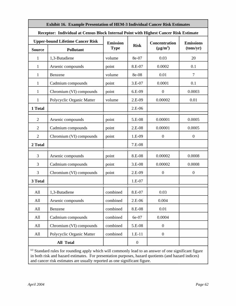
April 2004 Page 62
Exhibit 16. Example Presentation of HEM-3 Individual Cancer Risk Estimates
Receptor: Individual at Census Block Internal Point with Highest Cancer Risk Estimate
Upper-bound Lifetime Cancer Risk EmissionType Risk Concentration
(:g/m3)Emissions(tons/yr)Source Pollutant
1 1,3-Butadiene volume 8e-07 0.03 20
1 Arsenic compounds point 8.E-07 0.0002 0.1
1 Benzene volume 8e-08 0.01 7
1 Cadmium compounds point 3.E-07 0.0001 0.1
1 Chromium (VI) compounds point 6.E-09 0 0.0003
1 Polycyclic Organic Matter volume 2.E-09 0.00002 0.01
1 Total 2.E-06
2 Arsenic compounds point 5.E-08 0.00001 0.0005
2 Cadmium compounds point 2.E-08 0.00001 0.0005
2 Chromium (VI) compounds point 1.E-09 0 0
2 Total 7.E-08
3 Arsenic compounds point 8.E-08 0.00002 0.0008
3 Cadmium compounds point 3.E-08 0.00002 0.0008
3 Chromium (VI) compounds point 2.E-09 0 0
3 Total 1.E-07
All 1,3-Butadiene combined 8.E-07 0.03
All Arsenic compounds combined 2.E-06 0.004
All Benzene combined 8.E-08 0.01
All Cadmium compounds combined 6e-07 0.0004
All Chromium (VI) compounds combined 5.E-08 0
All Polycyclic Organic Matter combined 1.E-11 0
All Total 0(a) Standard rules for rounding apply which will commonly lead to an answer of one significant figurein both risk and hazard estimates. For presentation purposes, hazard quotients (and hazard indices)and cancer risk estimates are usually reported as one significant figure.
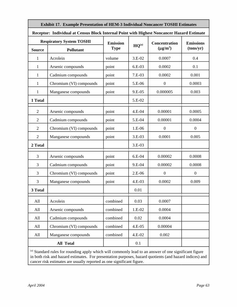
April 2004 Page 63
Exhibit 17. Example Presentation of HEM-3 Individual Noncancer TOSHI Estimates
Receptor: Individual at Census Block Internal Point with Highest Noncancer Hazard Estimate
Respiratory System TOSHI EmissionType HQ(a) Concentration
(:g/m3)Emissions(tons/yr)Source Pollutant
1 Acrolein volume 3.E-02 0.0007 0.4
1 Arsenic compounds point 6.E-03 0.0002 0.1
1 Cadmium compounds point 7.E-03 0.0002 0.001
1 Chromium (VI) compounds point 5.E-06 0 0.0003
1 Manganese compounds point 9.E-05 0.000005 0.003
1 Total 5.E-02
2 Arsenic compounds point 4.E-04 0.00001 0.0005
2 Cadmium compounds point 5.E-04 0.00001 0.0004
2 Chromium (VI) compounds point 1.E-06 0 0
2 Manganese compounds point 3.E-03 0.0001 0.005
2 Total 3.E-03
3 Arsenic compounds point 6.E-04 0.00002 0.0008
3 Cadmium compounds point 9.E-04 0.00002 0.0008
3 Chromium (VI) compounds point 2.E-06 0 0
3 Manganese compounds point 4.E-03 0.0002 0.009
3 Total 0.01
All Acrolein combined 0.03 0.0007
All Arsenic compounds combined 1.E-02 0.0004
All Cadmium compounds combined 0.02 0.0004
All Chromium (VI) compounds combined 4.E-05 0.00004
All Manganese compounds combined 4.E-02 0.002
All Total 0.1(a) Standard rules for rounding apply which will commonly lead to an answer of one significant figurein both risk and hazard estimates. For presentation purposes, hazard quotients (and hazard indices) andcancer risk estimates are usually reported as one significant figure.
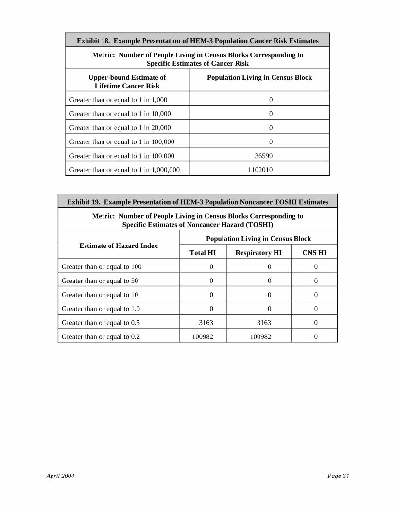
April 2004 Page 64
Exhibit 18. Example Presentation of HEM-3 Population Cancer Risk Estimates
Metric: Number of People Living in Census Blocks Corresponding toSpecific Estimates of Cancer Risk
Upper-bound Estimate ofLifetime Cancer Risk
Population Living in Census Block
Greater than or equal to 1 in 1,000 0
Greater than or equal to 1 in 10,000 0
Greater than or equal to 1 in 20,000 0
Greater than or equal to 1 in 100,000 0
Greater than or equal to 1 in 100,000 36599
Greater than or equal to 1 in 1,000,000 1102010
Exhibit 19. Example Presentation of HEM-3 Population Noncancer TOSHI Estimates
Metric: Number of People Living in Census Blocks Corresponding toSpecific Estimates of Noncancer Hazard (TOSHI)
Estimate of Hazard IndexPopulation Living in Census Block
Total HI Respiratory HI CNS HI
Greater than or equal to 100 0 0 0
Greater than or equal to 50 0 0 0
Greater than or equal to 10 0 0 0
Greater than or equal to 1.0 0 0 0
Greater than or equal to 0.5 3163 3163 0
Greater than or equal to 0.2 100982 100982 0
dThe “test memos” for a particular source category can be found on the NESHAPs page of EPA’s air toxicsweb site (http://www.epa.gov/ttn/atw/mactfnlalph.html) by selecting the source category and going to the residualrisk section of that page.
April 2004 Page 65
7.4.1 Reporting Results
A relatively simple summary can be used to report results, consistent with the need to make theresults both transparent and reproducible. Examples of reports prepared for EPA’s purposes canbe found in EPA’s residual risk “test memos;” these may or may not be appropriate examples forthe specific purposes of other risk assessments.(d) The summary generally will include thefollowing information:
• Documentation of input parameters, output spreadsheets, and risk characterization, withspecial emphasis on comparing estimated risks to risk targets;
• A simple presentation describing the assessment’s purpose (e.g., to determine whether risk isbelow levels of concern) and the outcome relative to that purpose (e.g., low risk is notdemonstrated); and
• Documentation of anything in the analysis that is discretionary, such as facility-specificemissions characteristics or choice of meteorological station. In particular, the rationale usedto select specific receptor locations and methods or calculations used to identify the locationassociated with the highest individual risk need to be documented.
7.4.2 Assessment and Presentation of Uncertainty
Risk managers need to understand the strengths and the limitations of the Tier 2 assessment. Acritical part of the risk characterization process, therefore, is an evaluation of the assumptions,limitations, and uncertainties inherent in the Tier 2 risk assessment in order to place the riskestimates in proper perspective.(3) Tier 2 risk assessments commonly include a quantitative orqualitative description of the uncertainty for each parameter and indicate the possible influenceof these uncertainties on the final risk estimates given knowledge of the models used. Tier 2assessments also may include a semi-quantitative sensitivity analyses. These approaches aredescribed in Section 5.4 above. Sensitivity analyses are discussed in more detail in Volume 1(Chapters 3 and 13) of this reference library.
7.5 Focusing Tier 3 on the Most Important HAPs/Sources
If cumulative cancer risk and/or noncancer hazard is above the level of concern, a Tier 3 analysismay be needed. This analysis may include all the sources and HAPs assessed in Tier 1, or maybe reduced to only those HAPs and sources of primary concern.
April 2004 Page 66
8.0 Tier 3 Inhalation Analysis
8.1 Introduction
This section describes an example approach for performing a Tier 3 inhalation risk assessment. Exhibit 20 provides an overview of this example approach. Tier 3 analyses are generally limitedto those HAPs and sources that collectively account for a large proportion of the potential riskor hazard estimated in Tier 2. The example Tier 3 assessment is significantly different than theexample Tier 1 and 2 approaches, in that it involves more complex dispersion modeling (e.g.,with ISCST3 or AERMOD), specific consideration of population locations, the use of anexposure model (TRIM.ExpoInhalation) to account for receptor behavior (e.g., time spent indifferent microenvironments), and use of a risk model (TRIM.RiskHH) to provide a more refinedcharacterization of risk, including multiple estimates of risk (e.g., central tendency and highend).
The Tier 3 analysis often involves considerable flexibility in analytical approach and detail. Thisexample includes the use of:
• A dispersion model (ISCST3 or AERMOD) to calculate hourly and annual averageconcentrations at user-specified exposure locations. ISCST3 allows considerable spatialrefinement in selecting exposure locations, and provides concentrations for user-specified(actual) locations.
• An exposure model (TRIM.ExpoInhalation) to combine air concentration information withhuman activity patterns to develop more precise, population- and site-specific exposureestimates. The user specifies the geographic area to be modeled, the number of individualsto be simulated to represent the study area population, and the demographic unit of resolutionfor the outputs. The model produces exposure estimates specific to modeled individual anddemographic unit (e.g., census tract or block, etc). Because the modeled individualsrepresent a random sample of the population of interest, the distribution of modeledindividual exposures can be extrapolated to the larger population.
• A risk model (TRIM.RiskHH) to calculate cumulative excess cancer risk and noncancerhazard associated with the modeled exposures. TRIM.RiskHH calculates human health riskmetrics, documents model inputs and assumptions, and displays results.
• Monitoring data may be used to evaluate or further characterize exposure concentration andexposure estimates.
The Tier 3 analysis may incorporate probabilistic inputs and model outputs using the TRIMmodeling system. If a potential regulatory action is involved, the scope, method, and inputs forprobabilistic modeling should be agreed to in advance with the appropriate regulatory agencies. It is recognized that there may be practical limitations that affect the scope, methods, inputs, oroutputs of the modeling:
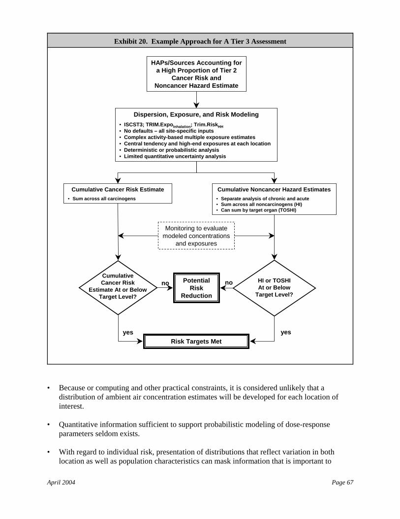
April 2004 Page 67
Dispersion, Exposure, and Risk Modeling• ISCST3; TRIM.ExpoInhalation; Trim.RiskHH• No defaults – all site-specific inputs• Complex activity-based multiple exposure estimates• Central tendency and high-end exposures at each location• Deterministic or probabilistic analysis• Limited quantitative uncertainty analysis
Cumulative Cancer Risk Estimate• Sum across all carcinogens
Cumulative Noncancer Hazard Estimates• Separate analysis of chronic and acute• Sum across all noncarcinogens (HI)• Can sum by target organ (TOSHI)
Potential Risk
Reduction
Risk Targets Met
no no
yesyes
HAPs/Sources Accounting for a High Proportion of Tier 2
Cancer Risk andNoncancer Hazard Estimate
Monitoring to evaluate modeled concentrations
and exposures
CumulativeCancer Risk
Estimate At or BelowTarget Level?
HI or TOSHIAt or Below
Target Level?
Exhibit 20. Example Approach for A Tier 3 Assessment
• Because or computing and other practical constraints, it is considered unlikely that adistribution of ambient air concentration estimates will be developed for each location ofinterest.
• Quantitative information sufficient to support probabilistic modeling of dose-responseparameters seldom exists.
• With regard to individual risk, presentation of distributions that reflect variation in bothlocation as well as population characteristics can mask information that is important to
April 2004 Page 68
decision making (e.g., locational variation is particularly relevant to source-specificassessment). Consequently, presentation of specific risk estimates across locations (e.g.,central tendency and high end estimates displayed via a geographical information system)separate from presentation of any distributions of risk estimates for each location arepreferred.
8.2 Fate and Transport Modeling
This example Tier 3 approach uses the ISCST3 model for estimating air concentrations for bothchronic and acute exposures. An alternative would be to use similar air quality model, such asAERMOD, when it becomes available. Other models may be appropriate for a specificfacility/source. The extent to which a specific air dispersion model is suitable for the evaluationof air toxic source impacts depends upon several factors, such as the nature of the pollutants(e.g., gaseous, particulate, reactive, inert), the meteorological and topographic complexities ofthe area, the complexity of the source distribution, the spatial scale and resolution required forthe analysis, and the level of detail and accuracy required for the analysis. For example, becauseof the assumption in Gaussian models of a steady wind speed and direction over the entiremodeling domain for each hour, the 50 km distance may be inappropriately long in many areas,especially where complex terrain or meteorology is present. In such cases a non-steady statemodel would be more appropriate.
Finer scale models, such as CAL3QHC and CALINE4, are most typically applied to exposurestudies from mobile sources. The UAM-TOX and CMAQ models are examples of modelswhich can simulate photochemically active air toxic species, including secondary formation ofpollutants like formaldehyde. Because the complex secondary formation processes are nonlinearand can occur at locations far distant from the emission source, these models are designed to beapplied to an exhaustive set of sources over a large region, rather than to individual facilities orsmall groups of facilities. The models more typically applied to single or multiple facilitiesinclude SCREEN3, ISCST3, ISCLT3, AERMOD, and CALPUFF. Brief descriptions of thesemodels are provided in Volume 1 (Chapter 9). Some modeling studies have combined theapplication of a regional model with a neighborhood-scale model in order to address secondaryand background concentration contributions, while capturing finer spatial resolution for primarypollutant predictions (see EPA’s Air Toxics Community Assessment and Risk ReductionProjects Databasehttp://yosemite.epa.gov/oar/CommunityAssessment.nsf/Welcome?OpenForm).
Where the assessment could support a regulatory decision, the use of an alternative modelcommonly is agreed to in advance with the regulatory agency decision-maker. Alternativemodels that conform to EPA’s air quality modeling guidance(17) are more likely to be acceptableto those decision-makers.
April 2004 Page 69
8.2.1 Model Inputs
Input data for ISCST3 falls into the same six categories used by HEM-3: (1) source location; (2)emissions data; (3) physical release parameters; (4) pollutant specific data (reactivity and dose-response data); (5) meteorological data; and (6) population data. Additional details are providedin the ISC model user’s guide.(9)
• Source location. ISCST3 requires coordinate data (latitude and longitude) for each emissionsource in the analysis. Multiple sources can be modeled in the same ISCST3 run.
• Emissions data. The analysis generally benefits from the use of the highest-quality,site-specific emissions data available, including chemical speciation. With ISCST3, usershave many more options for characterizing emissions. For example, users have the option tospecify variable emission rate factors for sources whose emissions vary as a function of time(e.g., month, season, hour-of-day). In addition, settling velocity categories, mass fractions,and reflection coefficients may be specified for sources of large particulates that experiencesettling and removal during dispersion. The emissions profile(s) used for Tier 3 modelingcommonly reflect the expected pattern(s) of emissions over a reasonable period of time (e.g.,several years). Note that these profiles may differ for different sources within a singlefacility.
• Physical release parameters. Tier 3 assessments commonly use facility/source-specificvalues for all stack/vent parameter data, as appropriate for the type of source. These valuescommonly reflect the expected patterns of emissions used to develop the emissions profilesfor modeling.
• Atmospheric reactivities of chemicals. Tier 3 assessments often are focused on a relativelysmall number of HAPs and sources that collectively account for a large proportion of the riskand/or hazard estimated in lower-tier analyses. Therefore, it may be worthwhile to considerreactivity and deposition in Tier 3 assessments. However, because the highest inhalationexposures are generally near to sources, these processes may not substantially influenceexposures unless they are very rapid. Exhibit 21 below provides a list of HAPs withatmospheric half-lives of one hour or less, for which considering reactivity may be useful. Volume I of this reference manual (Chapter 17) provides more data sources for half-life data. Atmospheric degradation in ISTST3 is limited to a first order approximation. ISCST3 canalso consider wet and dry deposition, but requires source- and HAP-specific information(e.g., on particle size and mass and solubility). As noted earlier, for HAPs with a significantpotential to form reaction products in the atmosphere, either a different model should beused, or the analysis should note the added uncertainties in not modeling these reactionproducts.
• Meteorology. Tier 3 analyses commonly use the most recent consecutive 5 years offacility/source-specific data from the nearest representative meteorological station. “Representative” generally means that the sources being modeled and the weather station arelocated in the same general environment with respect to significant terrain (e.g., valley vs.plateau), significant geographic features (e.g., proximity to a large body of water), andprevailing winds (i.e., similar wind rose/direction of dominant wind). Documentation
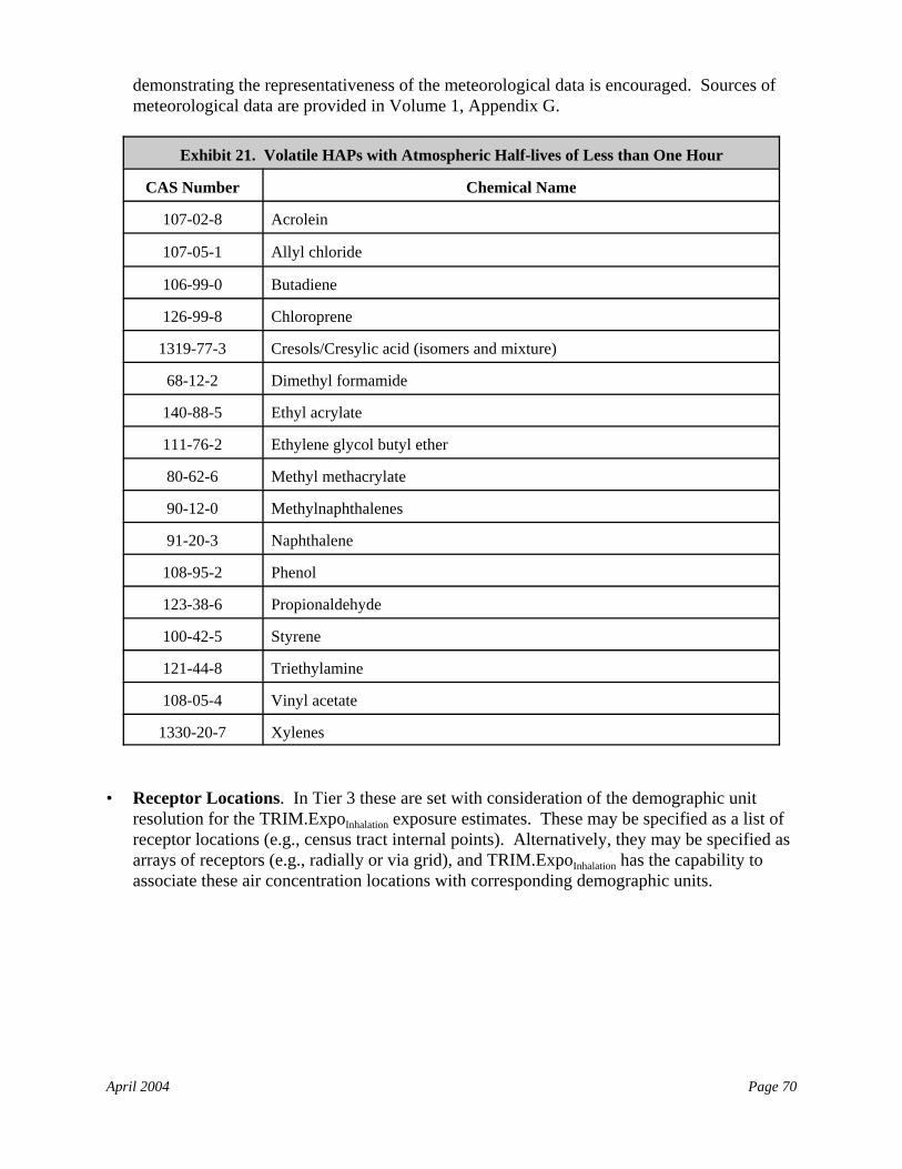
April 2004 Page 70
demonstrating the representativeness of the meteorological data is encouraged. Sources ofmeteorological data are provided in Volume 1, Appendix G.
Exhibit 21. Volatile HAPs with Atmospheric Half-lives of Less than One Hour
CAS Number Chemical Name
107-02-8 Acrolein
107-05-1 Allyl chloride
106-99-0 Butadiene
126-99-8 Chloroprene
1319-77-3 Cresols/Cresylic acid (isomers and mixture)
68-12-2 Dimethyl formamide
140-88-5 Ethyl acrylate
111-76-2 Ethylene glycol butyl ether
80-62-6 Methyl methacrylate
90-12-0 Methylnaphthalenes
91-20-3 Naphthalene
108-95-2 Phenol
123-38-6 Propionaldehyde
100-42-5 Styrene
121-44-8 Triethylamine
108-05-4 Vinyl acetate
1330-20-7 Xylenes
• Receptor Locations. In Tier 3 these are set with consideration of the demographic unitresolution for the TRIM.ExpoInhalation exposure estimates. These may be specified as a list ofreceptor locations (e.g., census tract internal points). Alternatively, they may be specified asarrays of receptors (e.g., radially or via grid), and TRIM.ExpoInhalation has the capability toassociate these air concentration locations with corresponding demographic units.
April 2004 Page 71
8.2.2 Model Runs
Using one complete year of meteorological data, ISCST3 calculates an ambient concentration foreach receptor location (district) specified in a run, for each hour of a one-year run. The ISCSTmodel can be run for single or multiple years. To obtain results for multiple years ofmeteorological data, separate ISCST3 model runs commonly are completed for each year. Basedon these results, ISCST3 can provide average ambient concentration for each modeled locationfor the time periods of interest (e.g., 1 hour to 5 years).
These concentrations are used to prepare inventories of chemical concentrations at each specifiedexposure location at selected time intervals (e.g., days, hours). The specific ISCST3 modeloutputs used to prepare inventories of chemical concentrations may depend on how the analysisis structured. As a general guideline:
• For cancer effects, calculate an annual average concentration using the one-hourconcentrations for each of the five years;
• For chronic noncancer effects, calculate an annual average concentration using the highestrolling annual average of one-hour concentrations for the five years; and
• For acute noncancer effects, identify the highest one-hour concentration in all five years.
8.3 Exposure Assessment
In this example Tier 3 approach, the exposure model (TRIM.ExpoInhalation) is used to combine theair concentration estimates with human activity patterns to develop more precise, population-and site-specific exposure estimates. The user specifies the geographic area to be modeled, thenumber of individuals to be simulated to represent the study area population, and thedemographic unit of resolution for the outputs. TRIM.ExpoInhalation generates a personal profilefor each simulated person that specifies various parameter variables required by the model. Themodel next uses diary-derived time/activity data matched to each personal profile to generate anexposure event sequence (also referred to as an “activity pattern” or “composite diary”) for themodeled individual that spans a specified time period, such as one year. Each event in thesequence specifies a start time, an exposure duration, a geographic location, a microenvironment,and an activity. Probabilistic algorithms are used to estimate the pollutant concentrationassociated with each exposure event. The estimated pollutant concentrations account for theeffects of ambient (outdoor) pollutant concentration, penetration factors, air exchange rates,decay/deposition rates, and proximity to emission sources, depending on the microenvironment,available data, and the estimation method selected by the user. The model produces adistribution of exposure estimates for the individuals modeled for each demographic unit (e.g.,census tract or block).
Major aspects of the set up and execution of the TRIM.ExpoInhalation model are described inseparate subsections below. The TRIM.ExpoInhalation User’s Document provides additionaldetails.(10) Where the assessment could support a regulatory decision, advance discussions withthe regulatory agency risk manager are encouraged to confirm the approach to be employed forthe exposure assessment.
April 2004 Page 72
8.3.1 Characterization of the Study Area
The study area will have been considered in the design of the air quality modeling step,including the resolution desired for the demographic unit for which exposure estimates are to begenerated. In the exposure modeling step, the user will confirm the extent of the study area forwhich air quality estimates are available, and the demographic unit scale at which exposureestimates are to be generated.
If the air quality modeling was designed to yield ambient concentration estimates associated withthe demographic units of interest for the exposure assessment (e.g., air concentration estimates atcensus tract/block centroids), TRIM.Expo will use those locations directly for developingpopulation specific exposure estimates. Otherwise, TRIM.Expo will assign the air qualityestimates to demographic units based on the distance between the location of each air qualityestimate and the geographic center of each demographic unit.
In TRIM.ExpoInhalation, the geographic units for the demographic data are called sectors. Themodel uses the demographic data to create personal profiles at the sector level. For each sectorthe model requires demographic information representing the distribution of age, gender, race,and work status within the study population. The initial release of TRIM.ExpoInhalation has inputfiles that already contain this demographic and location data for all Census tracts in the 50United States based on the 2000 Census. This database enables the user to model any study areain the country without having to make any changes to these input files. Finer scales, such asCensus block groups and blocks may be used with correspondingly suitable population data files. If fewer (thus larger) sectors were desired, the existing population data files could be aggregatedto larger regions.
The spatial units for the ambient air quality estimates are called districts. These are the areasassociated with each air quality estimate. As mentioned earlier, the air quality modeling may bedesigned so that the districts are the same as the sectors. For example, the air quality modelingmay produce estimates for census tract centroids and census tracts may be the sectors to be usedin the exposure modeling. If, however, the air quality estimate locations are not synonymouswith the sector centers, TRIM.Expo will assign the air quality districts to sectors based ondistance between their geographic centers (or other user-specified point). Each sector isassigned the air quality district for which this distance is shortest, yet within a user-specifiedmaximum distance. Sectors falling outside that distance are not modeled.
Another spatial unit in TRIM.Expo is the temperature zone, which may be used by the model toassign activity diaries to personal profiles (e.g., summer activities in summer weather) for themodeled individuals (see Section 8.3.2), and to specify parameters pertaining tomicroenvironments (e.g., aspects of climate control systems). The demographic sectors areassigned to temperature zones in similar fashion to the air quality district assignments (e.g., byclosest proximity of user-specified representative locations
In summary, the exposure assessment study area is composed of the demographic sectors forwhich air quality estimates (and temperature values) can been assigned.
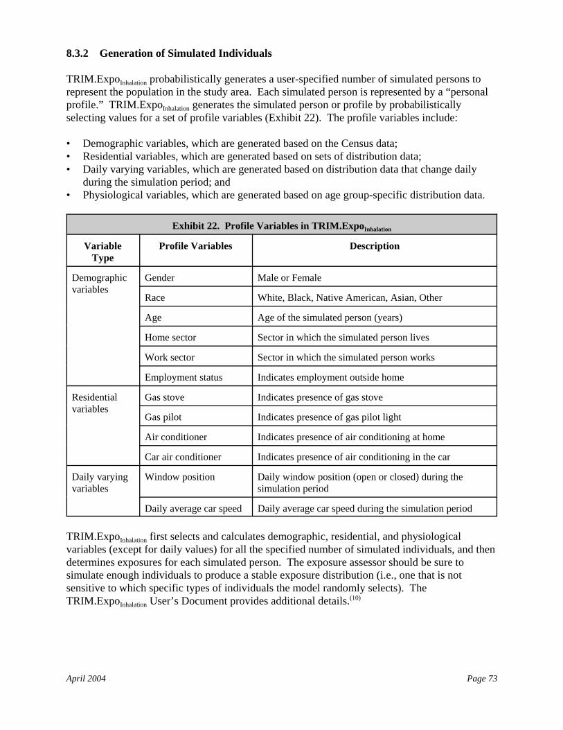
April 2004 Page 73
8.3.2 Generation of Simulated Individuals
TRIM.ExpoInhalation probabilistically generates a user-specified number of simulated persons torepresent the population in the study area. Each simulated person is represented by a “personalprofile.” TRIM.ExpoInhalation generates the simulated person or profile by probabilisticallyselecting values for a set of profile variables (Exhibit 22). The profile variables include:
• Demographic variables, which are generated based on the Census data;• Residential variables, which are generated based on sets of distribution data;• Daily varying variables, which are generated based on distribution data that change daily
during the simulation period; and• Physiological variables, which are generated based on age group-specific distribution data.
Exhibit 22. Profile Variables in TRIM.ExpoInhalation
VariableType
Profile Variables Description
Demographicvariables
Gender Male or Female
Race White, Black, Native American, Asian, Other
Age Age of the simulated person (years)
Home sector Sector in which the simulated person lives
Work sector Sector in which the simulated person works
Employment status Indicates employment outside home
Residentialvariables
Gas stove Indicates presence of gas stove
Gas pilot Indicates presence of gas pilot light
Air conditioner Indicates presence of air conditioning at home
Car air conditioner Indicates presence of air conditioning in the car
Daily varyingvariables
Window position Daily window position (open or closed) during thesimulation period
Daily average car speed Daily average car speed during the simulation period
TRIM.ExpoInhalation first selects and calculates demographic, residential, and physiologicalvariables (except for daily values) for all the specified number of simulated individuals, and thendetermines exposures for each simulated person. The exposure assessor should be sure tosimulate enough individuals to produce a stable exposure distribution (i.e., one that is notsensitive to which specific types of individuals the model randomly selects). TheTRIM.ExpoInhalation User’s Document provides additional details.(10)
April 2004 Page 74
8.3.3 Construction of A Sequence of Activity Events
TRIM.ExpoInhalation probabilistically creates a composite diary for each of the simulated personsby selecting a 24-hour diary record (a diary day) from an activity database for each day of thesimulation period. This diary is created based on the activity data in the Consolidated HumanActivities Database (CHAD).(18) CHAD data have been supplied with TRIM.ExpoInhalation for thispurpose. A composite diary is a sequence of events that simulate the movement of a modeledperson through geographical locations and microenvironments during the simulation period. Each event is defined by geographic location, start time, duration, microenvironment visited, andan activity performed. For the activity database, TRIM.ExpoInhalation currently provides a personalinformation file and an events file to summarize the CHAD data. These composite diaries arethen used in exposure concentration calculations.
8.3.4 Calculation of Concentrations in Microenvironments
TRIM.ExpoInhalation calculates ambient air concentrations in the various microenvironmentsvisited by the simulated person by using the ambient air data for the relevant sectors and theuser-specified method and parameters that are specific to each microenvironment.
TRIM.ExpoInhalation defines microenvironments by grouping the more than100 location codesdefined in the activity (CHAD) database into a smaller set of user-defined microenvironmentsamenable to modeling. The user has control over how many microenvironments will bemodeled, how they are defined, and what CHAD (or other activity database) locations should begrouped into each of microenvironment. The TRIM.ExpoInhalation User’s Document(10) lists the115 CHAD location codes included in TRIM.ExpoInhalation and the microenvironment to whicheach currently is assigned.
TRIM.ExpoInhalation calculates concentrations of the subject air pollutant in all themicroenvironments at each time step (e.g., hour) of the simulation period for each of thesimulated individuals, based on the user-provided hourly ambient air quality data specific to thegeographic locations visited by the individual. TRIM.ExpoInhalation provides two methods forcalculating microenvironmental concentrations: a mass balance method and a factors method(see Volume 1, Chapter 11). The user is required to specify a calculation method for each of themicroenvironments; some microenvironments can use one method while the rest use the other,without restrictions. The parameters, algorithms, and probabilistic elements used in each of themethods are explained in the TRIM.ExpoInhalation User’s Document.(10)
8.3.5 Estimating Exposure
TRIM.ExpoInhalation calculates exposure as a time series of exposure concentrations that a modeledindividual experiences during the simulation period. TRIM.ExpoInhalation determines the exposurebased on the air concentration in and minutes spent in each of a sequence of microenvironmentsvisited according to the composite diary. The exposure concentration at any clock hour duringthe simulation period is determined using the following equation:
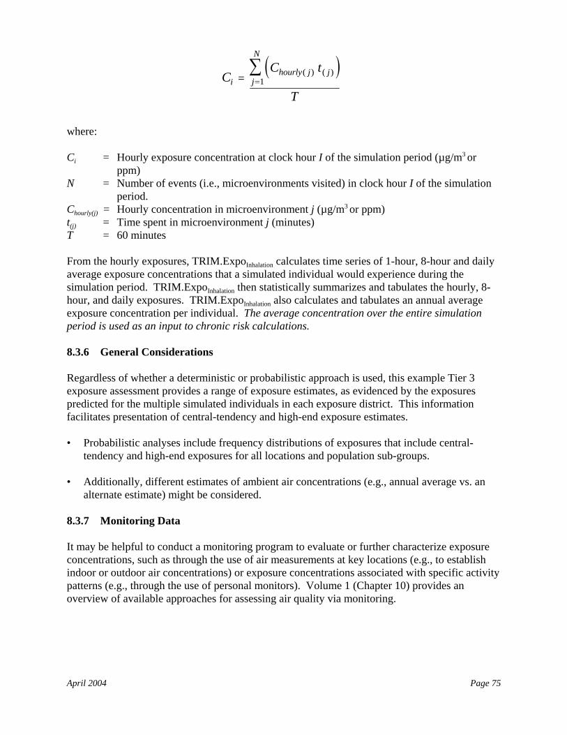
April 2004 Page 75
( )CC t
Ti
hourly j jj
N
= =∑ ( ) ( )
1
where:
Ci = Hourly exposure concentration at clock hour I of the simulation period (µg/m3 orppm)
N = Number of events (i.e., microenvironments visited) in clock hour I of the simulationperiod.
Chourly(j) = Hourly concentration in microenvironment j (µg/m3 or ppm)t(j) = Time spent in microenvironment j (minutes)T = 60 minutes
From the hourly exposures, TRIM.ExpoInhalation calculates time series of 1-hour, 8-hour and dailyaverage exposure concentrations that a simulated individual would experience during thesimulation period. TRIM.ExpoInhalation then statistically summarizes and tabulates the hourly, 8-hour, and daily exposures. TRIM.ExpoInhalation also calculates and tabulates an annual averageexposure concentration per individual. The average concentration over the entire simulationperiod is used as an input to chronic risk calculations. 8.3.6 General Considerations
Regardless of whether a deterministic or probabilistic approach is used, this example Tier 3exposure assessment provides a range of exposure estimates, as evidenced by the exposurespredicted for the multiple simulated individuals in each exposure district. This informationfacilitates presentation of central-tendency and high-end exposure estimates.
• Probabilistic analyses include frequency distributions of exposures that include central-tendency and high-end exposures for all locations and population sub-groups.
• Additionally, different estimates of ambient air concentrations (e.g., annual average vs. analternate estimate) might be considered.
8.3.7 Monitoring Data
It may be helpful to conduct a monitoring program to evaluate or further characterize exposureconcentrations, such as through the use of air measurements at key locations (e.g., to establishindoor or outdoor air concentrations) or exposure concentrations associated with specific activitypatterns (e.g., through the use of personal monitors). Volume 1 (Chapter 10) provides anoverview of available approaches for assessing air quality via monitoring.
April 2004 Page 76
8.4 Risk Characterization
For Tier 3, most risk estimates will be calculated automatically by TRIM.RiskHH, once themodeling scenarios are set up and run. The initial release of TRIM.RiskHH will calculate severalinhalation cancer risk and non-cancer hazard metrics at the individual and population level.
This example Tier 3 risk characterization considers background concentrations as appropriate(e.g., where the contribution of facility/source to risk is small compared to that of other sources. Note that consideration of background may or may not be appropriate pursuant to the specificlegal and regulatory authorities under which the risk assessment is being conducted.
8.4.1 Reporting Results
The initial release of TRIM.RiskHH will provide a visualization tool for presenting analysisresults in various automated formats. The risk assessor may want to utilize this tool to assistwith development of the risk characterization summary, which generally will include thefollowing information:
• Documentation of input parameters, outputs, and risk characterization, with special emphasison the range of risk or hazard estimates;
• A simple presentation describing the assessment’s purpose and the outcome relative to thepurpose (e.g., purpose: demonstrate that risk is below target levels; outcome: low risk notdemonstrated); and
• Documentation of all key assumptions or other inputs used for the assessment, such asemissions characteristics or choice of a nearby meteorological station. In particular, theassessor is encouraged to document the rationale used to define personal profiles and howthey are modeled and analyzed.
8.4.2 Assessment and Presentation of Uncertainty
Risk managers need to understand the strengths and the limitations of the Tier 3 assessment. Acritical part of the risk characterization process, therefore, is an evaluation of the assumptions,limitations, and uncertainties inherent in the Tier 3 risk assessment in order to place the riskestimates in proper perspective.(3) Tier 3 risk assessments commonly include semi-quantitativesensitivity analyses and quantitative uncertainty analysis (described in Section 5.4 above). Thegeneral quantitative approach to propagating or tracking uncertainty through probabilisticmodeling is described in Volume 1 (Chapter 31) of this reference library.
April 2004 Page 77
This section constitutes a snapshot of EPA’s current thinking and approach to the adaptation of theevolving methods of multipathway risk assessment to the context of Federal and state control of airtoxics. While inhalation risk assessment has been increasingly used in regulatory contexts over thelast several years, multipathway risk assessment tools are less well developed and field tested in aregulatory context. This section should be considered a living document for review and input. Bypublishing this portion of Volume 2 in its current state of development, EPA is soliciting theinvolvement of persons with experience in this field to help improve these assessment methods foruse in a regulatory context. EPA anticipates revisions to this draft section of Volume 2 on the basisof this input.
Chapter IV: Multipathway Risk Assessment
1.0 Introduction and Overview
This section describes an example approach for performing site-specific multipathway riskassessments for air toxics. These include an assessment of human health risks via ingestion (andperhaps other pathways/routes) as well as ecological risk assessment. Both types of assessmentsconsist of a tiered approach. A risk assessor may decide to complete only the lowest-tieranalysis that fits the purpose of the assessment (e.g., to determine that a facility’s cumulative riskis lower than a risk manager’s level of concern). Conversely, an assessor may choose not tocomplete a lower-tier analysis before completing a higher-tier analysis (e.g., the risk assessorcould go directly to Tier 3).
In this example approach, a multipathway risk assessment is conducted only if PB-HAPcompounds are present in facility/source emissions (see Exhibit 23), and acute exposures arenot assessed for multipathway analyses (although they may be for inhalation analyses). Thefocus is on exposure and risk/hazard once the PB-HAPs are deposited onto soils, into surfacewaters, etc. Other situations may warrant a multipathway analysis, such as when there aresignificant emissions of pollutants whose primary risk is through non-inhalation exposurepathways, or when state or local regulations require such analyses.
The discussion in this chapter is divided into the following sections:
• Section 2 provides an overview of the multipathway risk assessment and the tieredapproaches to the human health and ecological analyses;
• Section 3 provides information for preparing the emissions inventory for the multipathwayassessment;
• Section 4 describes an example approach for the multipathway human health riskassessment; and
• Section 5 provides an example approach for the ecological risk assessment.
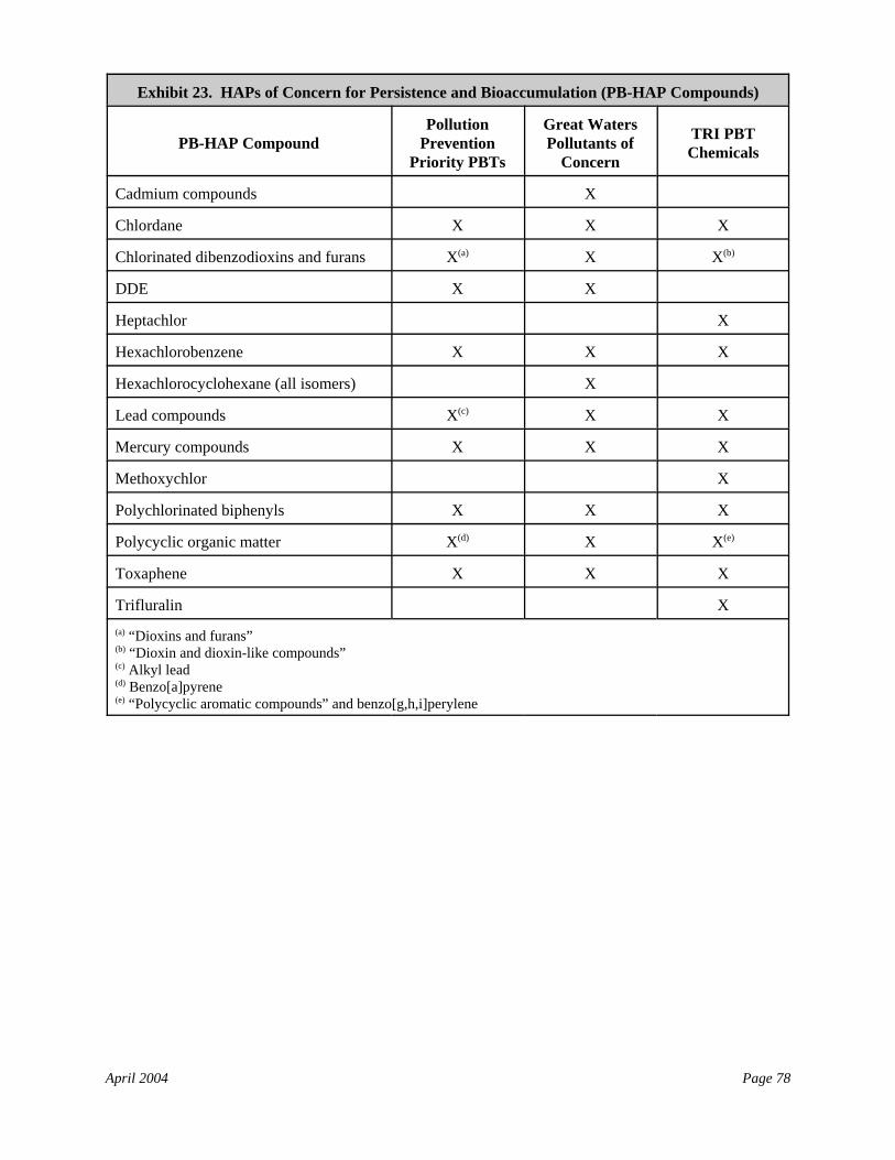
April 2004 Page 78
Exhibit 23. HAPs of Concern for Persistence and Bioaccumulation (PB-HAP Compounds)
PB-HAP CompoundPollution
PreventionPriority PBTs
Great WatersPollutants of
Concern
TRI PBTChemicals
Cadmium compounds X
Chlordane X X X
Chlorinated dibenzodioxins and furans X(a) X X(b)
DDE X X
Heptachlor X
Hexachlorobenzene X X X
Hexachlorocyclohexane (all isomers) X
Lead compounds X(c) X X
Mercury compounds X X X
Methoxychlor X
Polychlorinated biphenyls X X X
Polycyclic organic matter X(d) X X(e)
Toxaphene X X X
Trifluralin X(a) “Dioxins and furans”(b) “Dioxin and dioxin-like compounds”(c) Alkyl lead(d) Benzo[a]pyrene(e) “Polycyclic aromatic compounds” and benzo[g,h,i]perylene
April 2004 Page 79
2.0 Tiered Approach and Models Used
The example multipathway risk assessment approach currently includes only two tiers ofanalysis (Tier 2 and Tier 3, see Exhibit 24). EPA is investigating whether it is possible todevelop a Tier 1 methodology for multipathway analyses. Therefore, at this point in time, thisexample multipathway analysis starts with a Tier 2-level approach.
• Tier 1 is conceptualized as a simple look-up table or graph that identifies threshold emissionsrates (tons/year) for each PB-HAP compound below which multipathway risks are not ofconcern. The objective would be to allow a facility/source that emits small amounts of PB-HAP compounds to demonstrate that risk targets are met without the need for facility-specific modeling (as, for example, in a Tier 2 analysis). However, at this point in time, EPAdoes not have sufficient experience with multipathway air toxics risk assessments to developa Tier 1 approach.
• The example Tier 2 approach uses ISCST3 and the Methodology for Assessing HealthRisks Associated with Multiple Pathways of Exposure to Combuster (MPE) to estimateconcentrations in air, water, soil, and biota. For the human health assessment, MPE is usedto estimate cancer risk and noncancer hazard to a hypothetical receptor characterized using aconservative “subsistence farmer” scenario. For the ecological risk assessment,concentrations in air, water, and biota are compared to media-specific ecological toxicityreference values (i.e., a generic set of ecological receptors is assumed).
• The example Tier 3 approach uses the Total Risk Integrated Methodology (TRIM) in adeterministic or stochastic mode. TRIM Fate, Transport, and Ecological Exposure(TRIM.FaTE) is used to estimate concentrations in air, water, soil, and biota. For thehuman health risk assessment, TRIM.ExpoIngestion (coupled with a farm food chain model) isused to derive estimates of ingestion exposure for a set of scenarios (e.g., resident, farmer,fisher), and TRIM.RiskHH is used to derive cancer risk and chronic noncancer hazardestimates. For the ecological risk assessment, TRIM.RiskEco is used to derive estimates ofecological risk by comparing estimated concentrations of PB-HAPs in abiotic media, dietaryintakes, and body burdens to corresponding ecological toxicity reference values.
Although it is possible to evaluate acute exposures for the ingestion pathway, EPA does notgenerally recommend such assessments for substances released to the air because it is veryunlikely that acute ingestion threats could exist under typical release conditions and in theabsence of serious chronic ingestion risks. However, each assessment should consider theavailable evidence in making this judgment. The risk assessor is encouraged to state the reasonswhy an acute analysis for non-inhalation pathways was not performed.
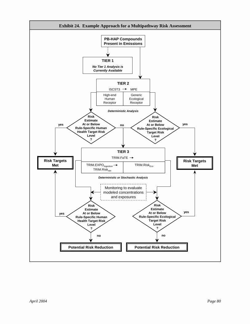
April 2004 Page 80
TIER 2ISCST3 MPE
High-end Human
Receptor
Generic Ecological Receptor
RiskEstimate
At or BelowRule-Specific Ecological
Target RiskLevel
?
RiskEstimate
At or BelowRule-Specific Human
Health Target RiskLevel
?
no
yes
Risk Targets Met
Potential Risk Reduction
PB-HAP Compounds Present in Emissions
TIER 1No Tier 1 Analysis isCurrently Available
no
Potential Risk Reduction
Risk Targets Met
no
yes
yes yes
Deterministic or Stochastic Analysis
Deterministic Analysis
TIER 3TRIM.FaTE
TRIM.EXPOIngestionTRIM.RiskHH
TRIM.RiskEco
Monitoring to evaluate modeled concentrations
and exposures
RiskEstimate
At or BelowRule-Specific Human
Health Target RiskLevel
?
RiskEstimate
At or BelowRule-Specific Ecological
Target RiskLevel
?
Exhibit 24. Example Approach for a Multipathway Risk Assessment
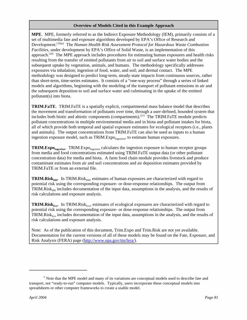
e Note that the MPE model and many of its variations are conceptual models used to describe fate andtransport, not “ready-to-run” computer models. Typically, users incorporate these conceptual models intospreadsheets or other computer frameworks to create a usable model.
April 2004 Page 81
Overview of Models Cited in this Example Approach
MPE. MPE, formerly referred to as the Indirect Exposure Methodology (IEM), primarily consists of aset of multimedia fate and exposure algorithms developed by EPA’s Office of Research andDevelopment.(19)(e) The Human Health Risk Assessment Protocol for Hazardous Waste CombustionFacilities, under development by EPA’s Office of Solid Waste, is an implementation of thisapproach.(20) The MPE approach includes procedures for estimating human exposures and health risksresulting from the transfer of emitted pollutants from air to soil and surface water bodies and thesubsequent uptake by vegetation, animals, and humans. The methodology specifically addressesexposures via inhalation; ingestion of food, water, and soil; and dermal contact. The MPEmethodology was designed to predict long-term, steady-state impacts from continuous sources, ratherthan short-term, time-series estimates. It consists of a “one-way process” through a series of linkedmodels and algorithms, beginning with the modeling of the transport of pollutant emissions in air andthe subsequent deposition to soil and surface water and culminating in the uptake of the emittedpollutant(s) into biota.
TRIM.FaTE. TRIM.FaTE is a spatially explicit, compartmental mass balance model that describesthe movement and transformation of pollutants over time, through a user-defined, bounded system thatincludes both biotic and abiotic components (compartments).(21) The TRIM.FaTE module predictspollutant concentrations in multiple environmental media and in biota and pollutant intakes for biota,all of which provide both temporal and spatial exposure estimates for ecological receptors (i.e., plantsand animals). The output concentrations from TRIM.FaTE can also be used as inputs to a humaningestion exposure model, such as TRIM.ExpoIngestion, to estimate human exposures.
TRIM.ExpoIngestion. TRIM.ExpoIngestion calculates the ingestion exposure to human receptor groupsfrom media and food concentrations estimated using TRIM.FaTE output data (or other pollutantconcentration data) for media and biota. A farm food chain module provides livestock and producecontaminant estimates from air and soil concentrations and air deposition estimates provided byTRIM.FaTE or from an external file.
TRIM.RiskHH. In TRIM.RiskHH, estimates of human exposures are characterized with regard topotential risk using the corresponding exposure- or dose-response relationships. The output fromTRIM.RiskHH includes documentation of the input data, assumptions in the analysis, and the results ofrisk calculations and exposure analysis.
TRIM.RiskEco. In TRIM.RiskEco, estimates of ecological exposures are characterized with regard topotential risk using the corresponding exposure- or dose-response relationships. The output fromTRIM.RiskEco includes documentation of the input data, assumptions in the analysis, and the results ofrisk calculations and exposure analysis.
Note: As of the publication of this document, Trim.Expo and Trim.Risk are not yet available. Documentation for the current versions of all of these models may be found on the Fate, Exposure, andRisk Analysis (FERA) page (http://www.epa.gov/ttn/fera/).
April 2004 Page 82
3.0 Developing the Emissions Inventory for Multipathway Analyses
As with the inhalation analysis, developing the emissions inventory involves (1) quantifyingemissions rates; (2) quantifying other emissions parameters important for the exposureassessment (e.g., temperature, stack height); (3) identifying the chemical species of the emittedHAPs (where applicable); and (4) identification of background concentrations of the HAPs beingreleased (in some instances).
As with inhalation, the risk assessor is encouraged to use its highest quality, most detailedemissions data. Acceptable data, in order by preference, include (1) actual measured emissionsfrom a recent high-activity, high-emission year, (2) measured emissions extrapolated to a high-activity, high-emission year, (3) facility/source-specific engineering estimates of a high-activity,high emission year (with documentation); and (4) permitted emissions, (e.g., the maximumallowed under MACT, or under a permit) with documentation that the permitted limits are notexceeded.
In general, if lower quality data (i.e., of types (3) and (4) above) are used, these data commonlyrepresent high-end estimates of emissions in order to ensure the assessment will produce health-protective results. The inventories commonly include the following release parameters for eachHAP released from each source: volume, schedule, emission factors, and applicable timeperiods. Emissions commonly represent conditions typical of a high-activity, high-emissionyear.
In this example approach, the risk assessments consider emissions controls in use at thefacility/source. At the least, the default assumption is that the facility’s sources are incompliance with the appropriate MACT standards and permit requirements, although it may bereasonable to modify this assumption if additional emissions controls are in place. Thedocumentation for the assessment includes the specific emissions inventories used.
4.0 Multipathway Human Health Risk Assessment
4.1 Introduction and Overview
The multipathway human health risk assessment is divided into two tiers, beginning with Tier 2:
• This example Tier 2 analysis uses the ISCST3 model and the MPE methodology(19) toestimate risk/hazard at the most impacted location via several ingestion pathways. TheHuman Health Risk Assessment Protocol for Hazardous Waste Combustion Facilities(HHRAP),(20) under development by EPA’s Office of Solid Waste, is an implementation ofthe MPE approach. Modeled deposition rates (from ISCST3) are converted by MPE intochemical concentrations in media and biota. MPE then uses exposure scenarios (e.g.,resident, farmer, fisher) to estimate exposure. Monitoring is not included explicitly in thisexample Tier 2 analysis because it is intended as a health-protective analysis.
• This example Tier 3 analysis uses TRIM.FaTE, TRIM.ExpoIngestion, and TRIM.RiskHH, toestimate ingestion risk/hazard (see Exhibit 25). The initial version of TRIM.ExpoIngestion usesa scenario-based approach to model exposure. In TRIM RiskHH, estimates of human
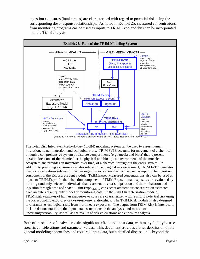
April 2004 Page 83
TRIM.FaTE(Fate, Transport &
Ecological Exposure)
TRIM.Risk(Risk Characterization)
FarmFood Chain
Quantitative risk & exposure characterization, U/V, assumptions, limitations, …
LIBRARY -Inputs (e.g., physical/chemical properties,site-specific data,
alt algorithms, etc)
Inputs:e.g., Activity data, population data,indoor:outdoor concentrations, etc)
HH Tox Database –Inputs:human health -dose-response assessments- (e.g., RfC, URE)
Eco ToxDatabaseInputs:Ecological effectsAssessments(e.g.,
endpoints, criteria)
EcoHH
----- MULTI-MEDIA IMPACTS -----
IngestionInhalation
TRIM.Expo(Human Exposure Event)
----- AIR-only IMPACTS --------------
AQ ModelOr
AQ Data
Alternative Exposure Model (e.g., HAPEM)
[Inhalation Risk] [Ingestion Risk] [Eco Risk]
ingestion exposures (intake rates) are characterized with regard to potential risk using thecorresponding dose-response relationships. As noted in Exhibit 25, measured concentrationsfrom monitoring programs can be used as inputs to TRIM.Expo and thus can be incorporatedinto the Tier 3 analysis.
Exhibit 25. Role of the TRIM Modeling System
The Total Risk Integrated Methodology (TRIM) modeling system can be used to assess humaninhalation, human ingestion, and ecological risks. TRIM.FaTE accounts for movement of a chemicalthrough a comprehensive system of discrete compartments (e.g., media and biota) that representpossible locations of the chemical in the physical and biological environments of the modeledecosystem and provides an inventory, over time, of a chemical throughout the entire system. Inaddition to providing exposure estimates relevant to ecological risk assessment, TRIM.FaTE generatesmedia concentrations relevant to human ingestion exposures that can be used as input to the ingestioncomponent of the Exposure-Event module, TRIM.Expo. Measured concentrations also can be used asinputs to TRIM.Expo. In the inhalation component of TRIM.Expo, human exposures are evaluated bytracking randomly selected individuals that represent an area’s population and their inhalation andingestion through time and space. Trim.ExpoInhalation can accept ambient air concentration estimatesfrom an external air quality model or monitoring data. In the Risk Characterization module,TRIM.Risk estimates of human exposures or doses are characterized with regard to potential risk usingthe corresponding exposure- or dose-response relationships. The TRIM.Risk module is also designedto characterize ecological risks from multimedia exposures. The output from TRIM.Risk is intended toinclude documentation of the input data, assumptions in the analysis, and metrics ofuncertainty/variability, as well as the results of risk calculations and exposure analysis.
Both of these tiers of analysis require significant effort and input data, with many facility/source-specific considerations and parameter values. This document provides a brief description of thegeneral modeling approaches and required input data, but a detailed discussion is beyond the
April 2004 Page 84
scope of this document. Such information can be found in user’s guides and relateddocumentation on EPA’s Fate, Exposure, and Risk Analysis (FERA) web page(http://www.epa.gov/ttn/fera/). Where the risk assessment involves a regulatory decision, therisk assessor is encouraged to discuss the scope, modeling/monitoring approach, and input datawith the appropriate regulatory authorities prior to conducting the analysis.
4.2 Pathways Evaluated
The example multipathway exposure assessment in this technical resource document focuses ontwo general categories of ingestion pathways. Incidental ingestion pathways consider exposuresthat may occur from ingestion of soils or surface water while engaged in other activities (e.g.,ingestion of soil while gardening or playing outside; ingestion of surface water whileswimming). Food chain pathways consider exposures that may occur if PB-HAP compoundsaccumulate in the food and water people consume. Exhibit 26 provides some examples of whichspecific pathways could be evaluated for each PB-HAP compound in a multipathway humanhealth assessment. As a general guideline, all of the pathways identified in the conceptual modelfor the assessment should be evaluated in the multipathway analysis. Note also that state andlocal agencies may have other recommended compounds and pathways required for analysis.
The focus of this example multipathway assessment is on ingestion pathways. Other exposurepathways may be important for particular risk assessments, including dermal exposures (i.e.,direct contact with contaminated soils, surface waters, or surface water sediments during outsideactivities such as gardening or swimming); resuspension of dust (e.g., from wind blowing acrosscontaminated soils) and subsequent inhalation of the dust particles; and ingestion ofcontaminated groundwater. However, EPA does not have sufficient experience withmultipathway air toxics risk assessments to identify the circumstances for which exposures viathese additional pathways may represent a potential concern. Each assessment may consider theavailable evidence in determining whether the risk assessment should include dermal exposure,resuspension of dust, and ingestion of groundwater. At a minimum, the risk characterizationshould state the reasons why an acute analysis for non-inhalation pathways was not performed.
• If facility/source-specific circumstances suggest that dermal pathways may be of concern,EPA’s Risk Assessment Guidance for Superfund (RAGS), Part E, Supplemental Guidance forDermal Risk Assessment,(22) includes a relatively straightforward methodology for dermalexposure and risk assessment, starting with soil concentrations. The Planning Tables in thedocument are simple to use and incorporate into the multipathway analysis.
• Relative to the direct inhalation pathway, inhalation of soil resulting from dust resuspensionby wind erosion generally is not a significant pathway of concern for air toxics riskassessments. If facility/source-specific circumstances suggest that resuspension of dust mayrepresent a potential concern, EPA’s MPE methodology(19) discusses the methods forevaluating this pathway.
• If facility/source-specific circumstances suggest that groundwater may represent a potentialconcern (e.g., the presence of extremely shallow aquifers used for drinking water purposes,or a karst environment in which the local surface water significantly affects the quality ofground water used as a drinking water source) the TRIM.FaTE library includes a
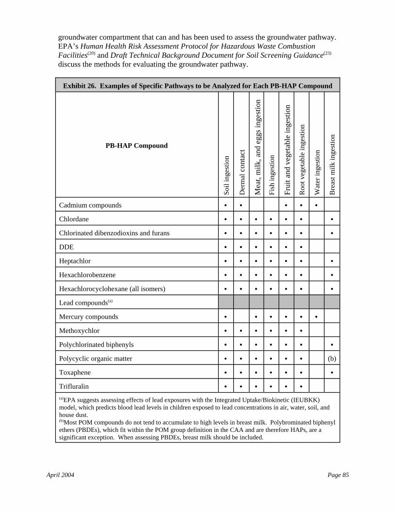
April 2004 Page 85
groundwater compartment that can and has been used to assess the groundwater pathway. EPA’s Human Health Risk Assessment Protocol for Hazardous Waste CombustionFacilities(20) and Draft Technical Background Document for Soil Screening Guidance(23)
discuss the methods for evaluating the groundwater pathway.
Exhibit 26. Examples of Specific Pathways to be Analyzed for Each PB-HAP Compound
PB-HAP Compound
Soil
inge
stio
n
Der
mal
con
tact
Mea
t, m
ilk, a
nd e
ggs i
nges
tion
Fish
inge
stio
n
Frui
t and
veg
etab
le in
gest
ion
Roo
t veg
etab
le in
gest
ion
Wat
er in
gest
ion
Bre
ast m
ilk in
gest
ion
Cadmium compounds C C C C C
Chlordane C C C C C C C
Chlorinated dibenzodioxins and furans C C C C C C C
DDE C C C C C C
Heptachlor C C C C C C C
Hexachlorobenzene C C C C C C C
Hexachlorocyclohexane (all isomers) C C C C C C C
Lead compounds(a)
Mercury compounds C C C C C C
Methoxychlor C C C C C C
Polychlorinated biphenyls C C C C C C C
Polycyclic organic matter C C C C C C (b)
Toxaphene C C C C C C C
Trifluralin C C C C C C
(a)EPA suggests assessing effects of lead exposures with the Integrated Uptake/Biokinetic (IEUBKK)model, which predicts blood lead levels in children exposed to lead concentrations in air, water, soil, andhouse dust.(b)Most POM compounds do not tend to accumulate to high levels in breast milk. Polybrominated biphenylethers (PBDEs), which fit within the POM group definition in the CAA and are therefore HAPs, are asignificant exception. When assessing PBDEs, breast milk should be included.
April 2004 Page 86
IEC CR
BWEF ED
AT=
××
×
4.3 Estimating Dietary Intake
The following generic equation is used calculate dietary chemical intake:(24) Volume 1 of thisReference Library (Chapter 20) provides a more detailed discussion of this equation.
where
I = Chemical intake rate, or the amount of pollutant ingested per unit time per unit bodymass, expressed in units of mg/kg-day. For evaluating exposure to noncarcinogens,the intake is referred to as Average Daily Dose (ADD); for evaluating exposure tocarcinogenic compounds, the intake is referred to as Lifetime Average Daily Dose(LADD)
Chemical-related variable:
EC = Exposure concentration of the chemical in the medium of concern for the time periodbeing analyzed, expressed in units of mg/kg for soil and food or mg/L for surfacewater or beverages (including milk)
Variables that describe the exposed population (also termed “intake variables”):
CR = Consumption rate, the amount of contaminated medium consumed per unit of time orevent (e.g., kg/day for food items and L/day for water)
EF = Exposure frequency (number of days exposed per year)ED = Exposure duration (number of years exposed )BW = Average body weight of the receptor over the exposure period (kg)
Assessment-determined variable:
AT = Averaging time, the period over which exposure is averaged (days). For carcinogens,the averaging time is 25,550 days, based on an assumed lifetime exposure of 70years; for noncarcinogens, averaging time equals ED (years) multiplied by 365 daysper year
• The exposure concentration (EC) for a chemical is calculated separately for each food itemand environmental medium of concern. The value of these variables is determined primarilyby modeling; however, monitoring data may be used to evaluate or further characterizeexposure concentrations at key locations considered (as noted earlier, where the riskassessment involves a regulatory decision, the risk assessor is encouraged to discuss thescope and approach for collecting monitoring data with the appropriate regulatory authoritiesprior to conducting the analysis).
• Consumption rate (CR) is the amount of contaminated food or medium consumed per eventor unit of time (e.g., amount of fish consumed per meal or per day). Note that consumption
April 2004 Page 87
rate changes with age (e.g., children and adults eat different amounts of the same food items). The consumption rate is usually calculated by first estimating the amount of a given mediumconsumed per unit time and then multiplying by a fraction of the total dietary intake for thistype of food or medium (e.g., 25 percent), representing the amount consumed from the studyarea. The specific fraction applied depends on the assumptions used for the analysis and canrange from zero to 100 percent. For example, if the analysis assumed an individualconsumed 6 grams of fish per day and obtained 25 percent of the fish from the contaminatedarea, CR would be 6 × .25 = 1.5 g/day.
• The specific exposure frequency (EF) specifies the number of days exposed each year,which generally ranges from a weekly or seasonal basis to 350 days/year (i.e., a person isresident in an area but spends two weeks each year in a different location, such as onvacation).
• Exposure duration (ED) is the length of time that a particular assessment represents (e.g., alifetime or a particular residence time). This is specified for each analysis.
• The choice of body weight (BW) for use in the exposure assessment depends on thedefinition of the person at potential risk. Because children have lower body weights, typicalingestion exposures per unit of body weight, such as for soil, milk, and fruits, aresubstantially higher for children. If a lifetime exposure duration (or an exposure durationover the childhood and adult years) is being evaluated, it needs to be based on differingvalues for the different age groups. If less than a lifetime exposure estimate is beingevaluated, it is important to include the children’s age group in the specific scenarios orcohorts used (see Volume 1, Chapter 20).
• Averaging time. When evaluating exposure to noncarcinogenic toxicants, intake isaveraged over the period of exposure. For carcinogens, intakes are traditionally calculatedby prorating the total cumulative dose over a lifetime (i.e., chronic daily intakes, also calledlifetime average daily intakes).
4.4 Ingestion Toxicity Assessment
As noted in Volume 1 of the reference library (Chapter 12), toxicity assessment is accomplishedin two steps: hazard identification and dose-response assessment. Dose-response values (e.g.,CPFs, RfDs) are used to estimate the potential for adverse impacts resulting from exposure to agiven concentration of a PB-HAP. Identifying critical human health endpoints (cancer vs.noncancer) and target organs is critical for structuring the multipathway risk assessment,including determining what ingestion exposure pathways are of potential concern and how tosum the risks from exposure to multiple HAPs. Volume 1 describes this process in greaterdetail. For each PB-HAP included in a risk assessment, the risk assessor should identify thecritical human health endpoints and target organs to ensure that cumulative risk across all HAPsis estimated in a manner consistent with risk assessment principles.
EPA/OAQPS has developed a set of recommended screening-level chronic human health dose-response values for many HAPs. This information is presented in Appendix C of Volume 1,which provides information on the type of hazard associated with each HAP (e.g., cancer,
April 2004 Page 88
non-cancer) and the applicable dose-response values for each HAP (e.g., RfCs, IURs). The mostup-to-date list of default screening level dose-response values recommended by EPA for the 188HAPs is provided at http://www.epa.gov/ttn/atw/toxsource/summary.html. Other dose-responsevalues that have undergone independent peer review may also be acceptable, but generallyshould be consistent with EPA risk assessment guidelines and agreed upon in advance forassessments that have regulatory implications. Descriptive information on the type of healthhazards associated with each HAP (e.g., cancer, noncancer) may be found athttp://www.epa.gov.ttn/atw/haptindex.html.
The oral cancer slope factor (CSF) is used to estimate ingestion cancer risk. It is derived in asimilar way as the inhalation unit risk estimate (IUR) (see Volume I of this reference library). The CSF is defined as the upper-bound excess lifetime cancer risk estimated to result fromcontinuous exposure to an agent. The true risk to humans, while not identifiable, is not likely toexceed the upper-bound estimate (the CSF). The CSF is presented as the risk of cancer per mgof intake of the substance per kg body weight per day (i.e., [mg/kg-day]-1).
The oral Reference Dose (RfD) is used to estimate hazard. The RfD is expressed as a chronicdietary intake level (in units of mg/kg-day). The RfD is an estimate (with uncertainty spanningperhaps an order of magnitude) of a continuous exposure to the human population (includingsensitive subgroups) that is likely to be without an appreciable risk of deleterious effects during alifetime. In other words, exposures at or below the RfD will probably not cause adverse healtheffects, even to sensitive subgroups. This generally is used in EPA’s health effects assessmentsfor effects other than cancer.
4.5 Risk Characterization for Ingestion Analysis
The process for characterizing cancer risks and noncancer hazards in this example multipathwayanalysis approach can be thought of as developing information to fill in a matrix similar to thatshown in Exhibit 27 in addition to the discussion of assumptions, limitations, and uncertaintiesthat are an essential part of risk characterization. A table like this would be developed for eachreceptor being evaluated (e.g., a scenario-based receptor or simulated individual) in the studyarea. This type of presentation format shows the aggregate risk for each chemical acrossmultiple pathways, the cumulative risk for each pathway across chemicals, and the overallcumulative cancer risk. In addition, this format allows one to quickly identify both theindividual chemicals and pathways that contribute most to the total risk estimate.
Definition of Terms in Ingestion Dose-Response Values
Oral Cancer Slope Factor (CSF): An upper bound, approximating a 95% confidence limit, on theincreased cancer risk from a lifetime exposure to an agent. This estimate is usually expressed in unitsof proportion (of a population) affected per mg/kg-day.
Reference Dose (RfD): An estimate (with uncertainty spanning perhaps an order of magnitude) of adaily oral exposure to the human population (including sensitive subgroups) that is likely to be withoutan appreciable risk of deleterious effects during a lifetime.
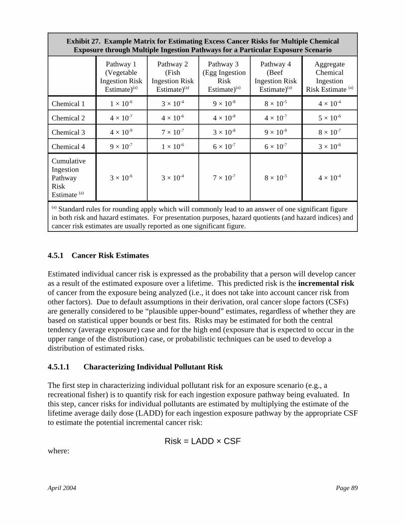
April 2004 Page 89
Exhibit 27. Example Matrix for Estimating Excess Cancer Risks for Multiple ChemicalExposure through Multiple Ingestion Pathways for a Particular Exposure Scenario
Pathway 1(Vegetable
Ingestion RiskEstimate)(a)
Pathway 2 (Fish
Ingestion RiskEstimate)(a)
Pathway 3 (Egg Ingestion
RiskEstimate)(a)
Pathway 4(Beef
Ingestion RiskEstimate)(a)
AggregateChemicalIngestion
Risk Estimate (a)
Chemical 1 1 × 10⁻⁶ 3 × 10⁻⁴ 9 × 10⁻⁸ 8 × 10⁻⁵ 4 × 10⁻⁴
Chemical 2 4 × 10⁻⁷ 4 × 10⁻⁶ 4 × 10⁻⁸ 4 × 10⁻⁷ 5 × 10⁻⁶
Chemical 3 4 × 10⁻⁹ 7 × 10⁻⁷ 3 × 10⁻⁸ 9 × 10⁻⁹ 8 × 10⁻⁷
Chemical 4 9 × 10⁻⁷ 1 × 10⁻⁶ 6 × 10⁻⁷ 6 × 10⁻⁷ 3 × 10⁻⁶
CumulativeIngestionPathwayRiskEstimate (a)
3 × 10⁻⁶ 3 × 10⁻⁴ 7 × 10⁻⁷ 8 × 10⁻⁵ 4 × 10⁻⁴
(a) Standard rules for rounding apply which will commonly lead to an answer of one significant figurein both risk and hazard estimates. For presentation purposes, hazard quotients (and hazard indices) andcancer risk estimates are usually reported as one significant figure.
4.5.1 Cancer Risk Estimates
Estimated individual cancer risk is expressed as the probability that a person will develop canceras a result of the estimated exposure over a lifetime. This predicted risk is the incremental riskof cancer from the exposure being analyzed (i.e., it does not take into account cancer risk fromother factors). Due to default assumptions in their derivation, oral cancer slope factors (CSFs)are generally considered to be “plausible upper-bound” estimates, regardless of whether they arebased on statistical upper bounds or best fits. Risks may be estimated for both the centraltendency (average exposure) case and for the high end (exposure that is expected to occur in theupper range of the distribution) case, or probabilistic techniques can be used to develop adistribution of estimated risks.
4.5.1.1 Characterizing Individual Pollutant Risk
The first step in characterizing individual pollutant risk for an exposure scenario (e.g., arecreational fisher) is to quantify risk for each ingestion exposure pathway being evaluated. Inthis step, cancer risks for individual pollutants are estimated by multiplying the estimate of thelifetime average daily dose (LADD) for each ingestion exposure pathway by the appropriate CSFto estimate the potential incremental cancer risk:
Risk = LADD × CSFwhere:
April 2004 Page 90
Risk = Individual cancer risk (expressed as an upper-bound risk of contracting cancerover a lifetime) for each pollutant via the ingestion pathway being evaluated(unitless);
LADD = Lifetime Average Daily Dietary Intake rate for the pollutant via theingestion pathway being evaluated (mg/kg-d); and
CSF = Oral Cancer Slope Factor for the pollutant via the ingestion pathway beingevaluated [(mg/kg-d)-1]
Estimates of cancer risk are usually expressed as a probability represented in scientific notationas a negative exponent of 10. For example, an additional upper bound risk of contracting cancerof 1 chance in 10,000 (or one additional person in 10,000) is written as 1x10⁻⁴. Because CSFsare typically upper-bound estimates, actual risks may be lower than predicted – note that “thetrue value of the risk is unknown and may be as low as zero.”(25)
In this example approach, risks are evaluated initially for individuals within the potentiallyexposed population. Population risks for the exposed population may also be estimated, whichmay be useful in estimating potential economic costs and benefits from risk reduction. Sensitivesubpopulations should also be considered, when possible. Estimates of incidence also arepossible, although in small populations, even a very high individual risk estimate may not yieldan estimated incidence above one case of cancer.
For carcinogens being assessed based on the assumption of nonlinear dose-response, for whichan RfD was derived that considers cancer as well as other effects, the hazard quotient approachis appropriate for risk characterization (see below). Where detailed information on carcinogenicmechanisms exists it may also be possible to estimate risk directly from a nonlinear low-doseextrapolation. This approach is supported by EPA’s Guidelines for Carcinogen RiskAssessment.(11)
4.5.1.2 Characterizing Risk from Exposure to Multiple Pollutants
By each exposure pathway of a scenario, exposure may be to multiple chemicals at the sametime rather than a single chemical; however, CSFs are usually available only for individualcompounds within a mixture. Consequently, a component-by-component approach is usuallyemployed.(14) The following equation estimates the predicted cumulative incremental individualcancer risk from multiple substances for a single exposure pathway, assuming additive effectsfrom simultaneous exposures to several carcinogens:
RiskT = Risk1 + Risk2 + .... + Riskiwhere:
RiskT = Cumulative individual ingestion cancer risk (expressed as an upper-bound risk ofcontracting cancer over a lifetime); and
Riski = Individual ingestion risk estimate for the ith substance.
In screening-level assessments of carcinogens for which there is an assumption of a linear dose-response, the cancer risks predicted for individual chemicals may be added to estimatecumulative cancer risk for each pathway. This approach is based on an assumption that the risks
April 2004 Page 91
associated with individual chemicals in the mixture are additive. In more refined assessments,the chemicals being assessed may be evaluated to determine whether effects from multiplechemicals are synergistic (greater than additive) or antagonistic (less than additive), althoughsufficient data for this evaluation are usually lacking. In those cases where CSFs are availablefor a chemical mixture of concern, risk characterization can be conducted on the mixture usingthe same procedures used for a single compound.
For carcinogens being assessed based on the assumption of nonlinear dose-response, for whichan RfD considering cancer as well as other effects has been derived, the hazard quotientapproach will be appropriate (see Volume 1, Chapter 12).
4.5.1.3 Combining Risk Estimates across Multiple Ingestion Pathways
To evaluate risks associated with the aggregate exposure to a single PB-HAP across multiplepathways of a given scenario, the individual pollutant cancer risk estimates may be summed foreach chemical across the multiple ingestion pathways assessed. Additionally, a cumulativemulti-pathway risk estimate may be derived by summing cumulative (multiple pollutant) cancerrisk estimates across the multiple ingestion pathways.
4.5.1.4 Evaluating Risk Estimates from Inhalation and Ingestion Exposures
Depending on the ingestion scenario, the inhalation pathway may also have been assessed. Insuch cases, it may be possible to obtain an overall estimate of risk across all pathways bycombining the inhalation exposures with the ingestion exposures. It is important to note,however, that the methods and assumptions used to derive the inhalation and ingestion risks maynot always yield compatible exposure scenarios. Consequently, it may be sufficient to simplyqualitatively consider any potential cumulative risk across routes. This is particularly importantwhen population-level (versus individual) risk estimates are being developed. For example, ascenario-based ingestion exposure assessment will not be easily amenable to producing estimatesof numbers of people at different risk levels, while a population-based inhalation assessmentmay be more appropriate. For example, it would generally not be appropriate to add aninhalation risk that presumes a 70-year exposure duration with an ingestion pathway thatpresumes a 30-year exposure duration. Any mismatching of exposure durations amongpathways in a multipathway assessment should be carefully considered. For this reason,combining any risk estimates across the ingestion and inhalation pathways is commonly doneonly by an experienced toxicologist.
4.5.2 Noncancer Hazard
For noncancer effects (as well as carcinogens being assessed based on the assumption ofnonlinear dose-response), ingestion exposure concentrations are compared to RfDs, which areestimates (with uncertainty spanning perhaps an order of magnitude) of a daily oral exposure tothe human population (including sensitive subgroups) that is likely to be without an appreciablerisk of deleterious noncancer effects during a lifetime.
As with carcinogens, the development of hazard quotients (HQs) for ingestion typically isperformed first for individual air toxics, then hazard indices (HIs) may be developed for multiple
April 2004 Page 92
pollutant exposures, and may be summed across pathways to develop multiple pathwaycumulative hazard estimates. An additional step in the multipathway analysis is to evaluate bothingestion and inhalation hazard estimates. These steps are described in separate subsectionsbelow.
4.5.2.1 Characterizing Individual Pollutant Hazard
The first step in characterizing individual pollutant hazard for an exposure scenario (e.g., arecreational fisher) is to quantify hazard for each pollutant being evaluated. For ingestionexposures, noncancer hazards are estimated by dividing the estimate of the Average Daily Dose(ADD) by the chronic oral RfD to yield a hazard quotient (HQ) for individual chemicals:
HQ = ADD ÷ RfDwhere:
HQ = The Hazard Quotient for the pollutant via each ingestion pathway being evaluated(unitless);
ADD = Estimate of the Average Daily Dietary Intake rate for the pollutant via theingestion pathway being evaluated (mg/kg-d); and
RfD = the corresponding reference dose for the pollutant via the ingestion pathway beingevaluated (mg/kg-d)
In screening assessments, which are routinely built around a particular year’s estimate ofemissions, the chronic exposure estimate may be based on a somewhat shorter than “chronic”exposure concentration estimate (e.g., the average annual concentration estimated by modeling),employing the simplifying assumption of continued similar conditions for a long-term period. Amore refined assessment might then include an estimate of exposure derived using informationfor the full chronic period of exposure time period (e.g., a lifetime or substantial portion of alifetime, refined emissions estimates over the long-term period). Based on the definition of the RfD, an HQ less than or equal to one indicates that adversenoncancer effects are not likely to occur. With exposures increasingly greater than the RfD (i.e.,HQs increasingly greater than one), the potential for adverse effects increases. However, the HQshould not be interpreted as a probability, because the overall chance of adverse effects does notincrease linearly as exposures exceed the RfD.
4.5.2.2 Multiple Pollutant Hazard
Noncancer health effects data are usually available only for individual compounds within amixture. In these cases, the individual HQs can be summed together to calculate a multi-pollutant hazard index (HI):
HI = HQ1 + HQ2 + ...+ HQiwhere:
HI = Hazard index; andHQi = Hazard quotient for the ith air toxic.
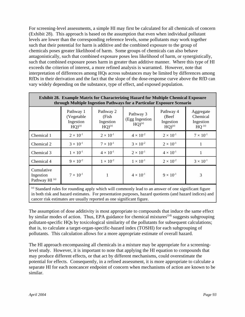
April 2004 Page 93
For screening-level assessments, a simple HI may first be calculated for all chemicals of concern(Exhibit 28). This approach is based on the assumption that even when individual pollutantlevels are lower than the corresponding reference levels, some pollutants may work togethersuch that their potential for harm is additive and the combined exposure to the group ofchemicals poses greater likelihood of harm. Some groups of chemicals can also behaveantagonistically, such that combined exposure poses less likelihood of harm, or synergistically,such that combined exposure poses harm in greater than additive manner. Where this type of HIexceeds the criterion of interest, a more refined analysis is warranted. However, note thatinterpretation of differences among HQs across substances may be limited by differences amongRfDs in their derivation and the fact that the slope of the dose-response curve above the RfD canvary widely depending on the substance, type of effect, and exposed population.
Exhibit 28. Example Matrix for Characterizing Hazard for Multiple Chemical Exposurethrough Multiple Ingestion Pathways for a Particular Exposure Scenario
Pathway 1(VegetableIngestion
HQ)(a)
Pathway 2 (Fish
IngestionHQ)(a)
Pathway 3 (Egg Ingestion
HQ)(a)
Pathway 4(Beef
IngestionHQ)(a)
AggregateChemicalIngestion
HQ (a)
Chemical 1 2 × 10⁻¹ 2 × 10⁻¹ 4 × 10⁻² 2 × 10⁻¹ 7 × 10⁻¹
Chemical 2 3 × 10⁻¹ 7 × 10⁻¹ 3 × 10⁻² 2 × 10⁻¹ 1
Chemical 3 1 × 10⁻¹ 4 × 10⁻¹ 2 × 10⁻¹ 4 × 10⁻¹ 1
Chemical 4 9 × 10⁻² 1 × 10⁻² 1 × 10⁻¹ 2 × 10⁻² 3 × 10⁻¹
CumulativeIngestionPathway HI (a)
7 × 10⁻¹ 1 4 × 10⁻¹ 9 × 10⁻¹ 3
(a) Standard rules for rounding apply which will commonly lead to an answer of one significant figurein both risk and hazard estimates. For presentation purposes, hazard quotients (and hazard indices) andcancer risk estimates are usually reported as one significant figure.
The assumption of dose additivity is most appropriate to compounds that induce the same effectby similar modes of action. Thus, EPA guidance for chemical mixtures(14) suggests subgroupingpollutant-specific HQs by toxicological similarity of the pollutants for subsequent calculations;that is, to calculate a target-organ-specific-hazard index (TOSHI) for each subgrouping ofpollutants. This calculation allows for a more appropriate estimate of overall hazard.
The HI approach encompassing all chemicals in a mixture may be appropriate for a screening-level study. However, it is important to note that applying the HI equation to compounds thatmay produce different effects, or that act by different mechanisms, could overestimate thepotential for effects. Consequently, in a refined assessment, it is more appropriate to calculate aseparate HI for each noncancer endpoint of concern when mechanisms of action are known to besimilar.
April 2004 Page 94
4.5.2.3 Evaluating Hazard Estimates From Inhalation and Ingestion Exposures
As with carcinogenic assessments, in some cases it may be possible to combine estimates ofinhalation hazard with ingestion hazard estimates to provide an estimate of total hazard across allexposure pathways for a receptor. As noted earlier, this is a complex analysis that generally isconducted by an experienced toxicologist.
4.5.3 Consideration of Long-Range Transport and Background
Although the example approach presented here focuses on populations located close to afacility/source, the contribution of a facility/source to deposition of PB-HAPs in more distantenvironmentally sensitive areas (e.g., the Great Lakes, Chesapeake Bay, the Florida Everglades)through long-range transport may also be a potential concern. Even small contributions from asingle facility may become significant over time. In addition, while local residents may not eatfish from bodies of water around a facility/source, fish caught from the large, productive lakesand bays in the U.S. are known to be eaten by significant numbers of people. Risk assessors areencouraged to discuss the contribution by an evaluated facility/source to the potential risksassociated with this exposure route.
Similarly, the study area around a specific facility/source may be subject to deposition of PB-HAPs resulting from long-range transport from more distant sources. Risk assessors areencouraged to discuss the contribution of these background levels of deposition as appropriate.
Note, however, that the local impacts of PB-HAP emissions may be of greatest potential concernfor many facilities/sources. Therefore, whether or not to include a detailed assessment of long-range transport and/or background generally is an analysis-specific decision (often determinedby legal and regulatory requirements).
4.5.4 Assessment and Presentation of Uncertainty
In the final part of this example risk characterization, estimates of cancer risk and noncancerhazard are presented in the context of uncertainties and limitations in the data and methodology. Exposure estimates and assumptions, toxicity estimates and assumptions, and the assessment ofuncertainty and variability commonly are discussed.
The risk estimates used in multipathway toxics risk assessments are unlikely to be fullyprobabilistic estimates of risk because of the numerous pathways, potential receptors, andpotential parameter values involved in the assessment. Rather, such risk estimates are likely tobe conditional estimates that incorporate a considerable number of assumptions about exposureand toxicity. Multipathway air toxics risk assessments are subject to additional sources ofuncertainty and variability as compared to inhalation risk assessments. The multimediamodeling effort is both more complex and less certain due to many factors. For example: (1)there are many more chemical-dependent and chemical-independent variables involved as inputvalues to the models; (2) the models involve analysis of the transfer of air toxics from the air toother media (e.g., soil, sediment, water), the subsequent movement of the air toxics betweenthese media (e.g., soil runoff to surface water), and uptake and metabolism by biota; and (3)many variables affect the ingestion of food, water, and other media by humans and wildlife, and
April 2004 Page 95
the exposure and risk estimates may differ considerably as a consequence of the assumptionsused to derive intake estimates. Sampling of biota and abiotic media also may be more complexand uncertain. Additional uncertainties are incorporated in the risk assessment when exposureestimates to multiple substances across multiple pathways are summed.
As a result of the increased complexity and uncertainty of the analytical approach, multipathwayrisk assessments commonly include semi-quantitative sensitivity analyses and may includequantitative uncertainty analysis. These approaches to uncertainty analysis are discussed ingreater detail in Section III-5.4 and in Volume 1 (Chapters 3 and 13) of this reference library.
4.6 Tier 1 Multipathway Human Health Analysis
(reserved)
April 2004 Page 96
4.7 Tier 2 Multipathway Human Health Analysis
4.7.1 Introduction
This section describes an example approach for performing a Tier 2 multipathway riskassessment. Exhibit 29 provides an overview of this example approach. In this exampleapproach, ISCST3 is used to provide deposition rates to soils and surface waters. The MPEmethodology is used to estimate human exposure at the most impacted location via severalingestion exposure pathways. Because EPA has not yet identified a Tier 1 approach, thisexample Tier 2 analysis incorporates simplified assumptions that allow a conservativerisk/hazard estimate to be calculated with a relatively modest analytical effort. If thefacility/source passes this screening analysis, the risk manager can be reasonably confident thatthe likelihood for significant risk/hazard is low. As a consequence, monitoring is not explicitlyincluded in this example Tier 2 analysis (although available monitoring data can be used asinputs to the exposure analysis).
4.7.2 Fate and Transport Modeling
This example Tier 2 approach uses the ISCST3 model for estimating air concentrations for bothchronic and acute exposures (an alternative would be to use AERMOD). Other models may berelevant for a specific facility/source. For example, if the facility/source is located in complexterrain and/or near a large body of water, other models may be more applicable (e.g., Cal-Pufffor complex terrain; non-Gaussian models for sources close to large bodies of water). Similarly,if the exposure point of concern is very near source (< 100-m) or very distant (> 50-km), othermodels would need to be applied (e.g., CALPUFF for > 50-km). However, where theassessment could support a regulatory decision, the use of an alternative model commonly isagreed to in advance with the regulatory agency decision-maker. Alternative models thatconform to EPA’s air quality modeling guidance(17) are more likely to be acceptable to thosedecision-makers.
4.7.2.1 Model Inputs
The modeling for the multipathway analysis commonly is executed in about the same way aswould be done for a Tier 2 inhalation analysis. For example, sources are characterized the sameway regarding stack/vent height and diameter, release temperature and velocity, flow rate, etc. The ISCST3 model requires the speciation profile of the emissions for ISCST3 in order tocalculate deposition rates properly. The risk assessor would have addressed deposition and theseproperties in the Tier 2 inhalation analysis if he/she executed the ISCST3 inhalation runs “withdepletion” (i.e., telling the model to subtract out the mass of chemical deposited). This is aconcern for emissions of chemicals that are predominantly particulates instead of vapors and/orare predominantly bound to particles (e.g., metals). However, the inhalation runs may not havebeen done with depletion, because it takes longer to do this. If the inhalation runs were donewithout depletion, they should be done again with depletion for the multipathway analysis.
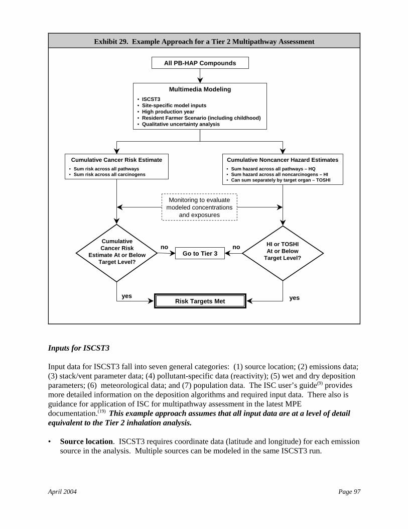
April 2004 Page 97
Multimedia Modeling• ISCST3• Site-specific model inputs• High production year• Resident Farmer Scenario (including childhood)• Qualitative uncertainty analysis
Go to Tier 3
Risk Targets Met
no
yes
Cumulative Cancer Risk Estimate• Sum risk across all pathways• Sum risk across all carcinogens
Cumulative Noncancer Hazard Estimates• Sum hazard across all pathways – HQ• Sum hazard across all noncarcinogens – HI• Can sum separately by target organ – TOSHI
no
yes
All PB-HAP Compounds
CumulativeCancer Risk
Estimate At or BelowTarget Level?
HI or TOSHIAt or Below
Target Level?
Monitoring to evaluate modeled concentrations
and exposures
Exhibit 29. Example Approach for a Tier 2 Multipathway Assessment
Inputs for ISCST3
Input data for ISCST3 fall into seven general categories: (1) source location; (2) emissions data;(3) stack/vent parameter data; (4) pollutant-specific data (reactivity); (5) wet and dry depositionparameters; (6) meteorological data; and (7) population data. The ISC user’s guide(9) providesmore detailed information on the deposition algorithms and required input data. There also isguidance for application of ISC for multipathway assessment in the latest MPEdocumentation.(19) This example approach assumes that all input data are at a level of detailequivalent to the Tier 2 inhalation analysis.
• Source location. ISCST3 requires coordinate data (latitude and longitude) for each emissionsource in the analysis. Multiple sources can be modeled in the same ISCST3 run.
April 2004 Page 98
• Emissions data. In this example approach, the risk assessor uses the best site-specificemissions data available, including chemical speciation. With ISCST3, users have manyoptions for characterizing emissions. For example, users have the option to specify variableemission rate factors for sources whose emissions vary as a function of time (e.g., month,season, hour-of-day). In addition, settling velocity categories, mass fractions, and reflectioncoefficients may be specified for sources of large particulates that experience settling andremoval during dispersion. Therefore, this example approach assumes that the emissionsprofile(s) used for modeling reflect the expected pattern(s) of emissions over a reasonableperiod of time (e.g., several years). Note that these profiles may differ for different sourceswithin a single facility.
• Stack/vent parameter data. Facility/source-specific values commonly are used for allstack/vent parameter data. These values commonly reflect the expected patterns of emissionsused to develop the emissions profiles for modeling.
• Atmospheric reactivities of chemicals. Atmospheric reactivities generally are not neededfor PB-HAP compounds.
• Wet and dry deposition parameters. The ISCST3 models requires the particulate/particle-bound/vapor fractions of the emissions in order to calculate wet and dry depositionof vapors and particles. These would probably be considered source-related, since althoughthey are chemical-dependent, they also vary by source (i.e., the industrial process affects theemissions profile).
For dry deposition of particles, the user needs to supply the following inputs (in addition tothe normal ISC inputs), including the:– Array of particle diameters of the emissions;– Array of mass fractions corresponding to the different particle diameters; and– Array of particle densities corresponding to the different particle diameters.
For wet deposition of particles, the user needs to supply the following inputs (in addition tothe normal ISC inputs), including the:– Particle scavenging coefficients for liquid precipitation corresponding to the different
particle diameters; and– Particle scavenging coefficients for frozen precipitation corresponding to the different
particle diameters.
For wet deposition of gases, the user needs to supply the following inputs (in addition to thenormal ISC inputs), including the:– Gaseous scavenging coefficient for liquid precipitation; and– Gaseous scavenging coefficient for frozen precipitation.
• Meteorology. Tier 2 multipathway analyses commonly use the most recent consecutive fiveyears of facility/source-specific data from the nearest representative meteorological station. “Representative” generally means that the sources being modeled and the weather station arelocated in the same general environment with respect to significant terrain (e.g., valley vs.plateau), significant geographic features (e.g., proximity to a large body of water), and
April 2004 Page 99
prevailing winds (i.e., similar wind rose/direction of dominant wind). Documentationdemonstrating the representativeness of the meteorological data is encouraged. Sources ofmeteorological data are provided in Volume 1, Appendix G.
• Population. Population is not defined for the ISCST3 model runs (population is definedusing MPE (see Section 4.7.3 below).
Inputs for the MPE Methodology
The MPE methodology requires air concentrations and deposition rates for the appropriatelocations as inputs. These are provided by ISCST3. A variety of additional chemical- and/orfacility/source-specific parameters are needed for MPE to calculate concentrations in variousmedia (e.g., soil, surface water) and biota (e.g., plants, fish). These are identified and describedin detail in the MPE documentation.(19)
4.7.2.2 Model Runs
Using one complete year of meteorological data, ISCST3 calculates annual deposition rates (orfluxes) for each receptor location specified in a run. Results for each of the five years ofmeteorological data are obtained using separate ISCST3 model runs for each year. ISCST3 canmodel all sources at the facility simultaneously; however, only one chemical can be modeled at atime. Therefore, for each PB-HAP compound, all sources of that compound could be modeled inthe same ISCST3 model run.
Defining receptor locations
For this example Tier 2 analysis, the subsistence farmer is assumed to occur at the modelinglocation (“node”) with the maximum deposition rate. Several iterations of the ISCST3 modelmay be required to locate this point. The risk assessor is encouraged to clearly document theprocess used to identify this point.
• If multiple PB-HAPs are present, the point where maximum deposition occurs for eachindividual PB-HAP may not be in the same location. This example approach assumes thatthese are all co-located (see Section 4.7.4 below).
• For this example approach, the point where maximum deposition occurs is used for all soilpathways and for the drinking water pathway.
• For surface water pathways, this example Tier 2 analysis is based on the surface water bodywithin the assessment area where maximum concentrations occur. This will depend on thelocation of the surface water bodies with respect to sources, characteristics of the surfacewater body (e.g., size, depth, flow rate), and characteristics of the watershed (e.g., size,runoff, erosion potential). Several water bodies/watersheds within the assessment area mayneed to be characterized in order to identify this water body. The risk assessor is encouragedto clearly document the process used to identify this water body.
April 2004 Page 100
• For this example approach, the subsistence farmer is assumed to fish in the water body wheremaximum concentrations occur.
Defining the duration of emissions
Because the concentrations of PB-HAP compounds often will slowly accumulate in soil,sediment, and biota over time, the total deposition over time (and the resulting mediaconcentrations) will depend on the specific duration of emissions selected for the analysis.
For a Tier 2 analysis, the duration of emissions used in the analysis commonly reflects theexpected duration of emissions from the facility/source being evaluated. A common duration is30 or 40 years (e.g., the expected lifespan of many facilities or processes). However, facilitiesmay continue to operate beyond their expected lifespan. Therefore, the risk assessor isencouraged to document the rationale for selecting a duration of emissions. In the absence ofclear rationale for another value, a conservative value (e.g., 100 years) can be selected.
Defining deposition/flux rates for estimating media concentrations
This example approach uses the average deposition/flux rates from the five years of ISCST3 modeling and assumes these rates are constant over the duration of emissions.
Model outputs to use
The modeled deposition rates and duration of deposition are used as inputs to the MPEmethodology to estimate PB-HAP concentrations in soil, water, and biota. This exampleapproach uses the average annual deposition rates as inputs to the MPE methodology.
4.7.3 Exposure Assessment
For this example Tier 2 assessment, the exposure assessment includes both central tendency andhigh end exposure estimates.
4.7.3.1 Characterization of the Study Population
For this example Tier 2 assessment, the study population is limited to a hypothetical subsistencefarmer assumed to reside at the point of maximum deposition and to fish in the water body withthe highest modeled concentrations. For assessments for which information of local farmingpractices is available, the location of actual farms can be used as the basis for a more realisticexposure scenario.
4.7.3.2 Defining the Point of Maximum Exposure
This example Tier 2 assessment defines the point of maximum exposure as follows:
• For a single PB-HAP compound, the point of maximum exposure is defined as the modeledlocation (node) at which the highest deposition rate occurs (soils) and the surface water body
April 2004 Page 101
with maximum modeled concentrations. Exposure estimates from these two locations aresummed to calculate total maximum exposure.
• For multiple PB-HAP compounds, the point of maximum exposure is defined by assumingthat the point of maximum exposure occurs at the same location for each PB-HAP compound(i.e., exposure for each compound is added to calculate total exposure).
4.7.3.3 Defining the Exposure Scenario
This example Tier 2 assessment is based on a single exposure scenario designed to provide aconservative estimate of risk/hazard via all ingestion pathways. This scenario is termed thesubsistence farmer. This scenario reflects an individual living on a farm and consuming meat,dairy products, and vegetables that the farm produces. All drinking water is obtained from asurface water body on the farm (or if no surface water is present, from collected rainfall). Theanimals raised on the farm subsist primarily on forage that is grown on the farm. This scenarioalso assumes that the farm family fishes in the surface water body with the highestconcentrations within the study area. They fish at a recreational level and eat the fish they catch. The maximum exposed individual is assumed to be exposed to PB-HAP compounds through thefollowing exposure pathways:
C Direct inhalation of vapors and particles (assessed during the inhalation analysis);C Incidental ingestion of soil and house dust;C Ingestion of drinking water from surface water sources;C Ingestion of homegrown produce;C Ingestion of home-produced meat, milk, and eggs; andC Ingestion of fish; andC Ingestion of breast milk (evaluated separately for an infant [for PCBs, dioxins, and furans]).
Within this general scenario, the specific exposure routes evaluated for a given facility/sourcemay depend on the particular PB-HAP compounds in the emissions being assessed (see Exhibit26).
4.7.3.4 Calculation of Exposure Concentration
This example Tier 2 approach calculates exposure concentration as follows:
• Exposure concentrations in soil, drinking water, and food items are calculated using theequations provided in the MPE methodology(19) or the HHRAP.(20)
• The maximum concentration (via each exposure pathway) reached during the modelingperiod is used as the exposure concentration. For a constant emissions scenario, this usuallywill be the final year of the modeling simulation (e.g., the last year the facility/source isexpected to operate).
• Note that existing monitoring data may be used to evaluate or refine the exposure estimatesbased on multimedia modeling.
April 2004 Page 102
4.7.3.5 Determining Exposure
This example Tier 2 approach assumes that the subsistence farmer is exposed to thisconcentration during his/her entire lifetime, from birth to the age of 70 years. This entails theuse of variable exposure factors (e.g., body weight, consumption rate) as the subsistence farmerages from birth to age 70. Additionally, for the derivation of chronic hazard estimates, a child(e.g., 0-7 years old) may be included to address the potential for substantially higher pollutant intake(in mg/kg-day) during those ages.
4.7.3.6 Determining Intake
For this example approach, the risk assessor calculates a central tendency and high end intake. EPA’s Exposure Factors Handbook(26) provides default central tendency and high-end values forintake and other exposure factors (e.g. body weight). Equations used to calculate intake arefound in the MPE methodology.(19) EPA’s Guidance on Selecting the Appropriate Age Groupsfor Assessing Childhood Exposures to Environmental Contaminants(27) and Child-SpecificExposure Factors Handbook(28) provide guidance on selecting the appropriate age groups toinclude for children and the exposure factors to use that are specific to each age group.
4.7.4 Risk Characterization
Risk characterization for this example Tier 2 approach is limited to estimating ingestion risk forthe subsistence farmer (calculated separately for cancer risk and chronic noncancer hazard). Theestimates of intake rates described in Section 4.7.3.6 are used to calculate risk and hazardaccording to the basic equations presented earlier in Section 4.5. Background concentrations arenot explicitly considered.
As noted earlier, the points of maximum deposition rates for multiple PB-HAPs are assumed tobe co-located, and the subsistence farm family is assumed to eat fish from the surface water bodywith the highest modeled concentrations.
4.7.4.1 Reporting Results
A relatively simple summary can be used to report results, as long as it is consistent with theneed to make the results both transparent and reproducible. Examples of reports prepared forEPA’s purposes can be found in EPA’s residual risk “test memos;” these may or may not beappropriate examples for the specific purposes of other risk assessments. The summarygenerally will include the following information:
• Documentation of input parameters, output values, and risk characterization, with specialemphasis on comparing estimated risk/hazard to risk targets;
• A simple presentation describing the assessment’s purpose (e.g., to determine whether risk isbelow levels of concern) and the outcome relative to that purpose (e.g., low risk is notdemonstrated); and
April 2004 Page 103
• Documentation of anything that is discretionary (i.e., anything that is facility-specific), suchas emissions characteristics or choice of a meteorological station other than the nearest.
4.7.4.2 Assessment and Presentation of Uncertainty
Risk managers need to understand the strengths and the limitations of the Tier 2 multipathwayrisk assessment. A critical part of the risk characterization process, therefore, is an evaluation ofthe assumptions, limitations, and uncertainties inherent in the Tier 2 assessment in order to placethe risk estimates in proper perspective.(3) Tier 2 assessments commonly include a quantitativeor qualitative description of the uncertainty for each parameter and indicating the possibleinfluence of these uncertainties on the final risk estimates given knowledge of the models used. Tier 2 assessments also may include a semi-quantitative sensitivity analyses. These approachesare described in Section III-5.4. Sensitivity analyses are discussed in more detail in Volume 1(Chapters 3 and 13) of this reference library.
4.7.5 Potential Refinements of a Tier 2 Approach
If the results of the Tier 2 assessment indicate that risk targets are not met, the risk assessor hasthe option of conducting a much more facility/source-specific, refined Tier 2 assessment usingthe ISCST3 model and MPE methodology. Refinements might include characterizing themodeling region in much greater detail and using exposure scenarios that are more realistic forthe facility/source setting (the exposure assessment for each scenario could still be based on thebasic equations found in the MPE methodology). Potential refinements might include:
• Defining and assessing a “resident” scenario based on modeled deposition rates at locationswhere people actually live (e.g., census tract internal points);
• For the “subsistence farmer,” (a) use an actual location of a farm within the study area (ratherthan assuming it is located at the point of maximum deposition), (b) more realisticallyincorporate only a subset of the potential pathways, and/or (c) assume that the farmer obtainssome of his/her food from other sources.
• When summing exposures over multiple pathways, use high-end concentrations for somepathways and central tendency concentrations for others.
• Incorporating a limited monitoring program to evaluate key exposure estimates (e.g.,concentrations of PB-HAPs in various food items).
A more complete listing of potential exposure scenarios is presented in Volume 1 (Part III) ofthis reference library. EPA’s Guidelines for Exposure Assessment(29) discusses how to developthese types of exposure scenarios.
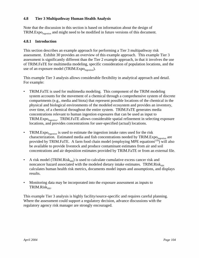
April 2004 Page 104
4.8 Tier 3 Multipathway Human Health Analysis
Note that the discussion in this section is based on information about the design ofTRIM.ExpoIngestion and might need to be modified in future versions of this document.
4.8.1 Introduction
This section describes an example approach for performing a Tier 3 multipathway riskassessment. Exhibit 30 provides an overview of this example approach. This example Tier 3assessment is significantly different than the Tier 2 example approach, in that it involves the useof TRIM.FaTE for multimedia modeling, specific consideration of population locations, and theuse of an exposure model (TRIM.ExpoIngestion).
This example Tier 3 analysis allows considerable flexibility in analytical approach and detail. For example:
• TRIM.FaTE is used for multimedia modeling. This component of the TRIM modelingsystem accounts for the movement of a chemical through a comprehensive system of discretecompartments (e.g., media and biota) that represent possible locations of the chemical in thephysical and biological environments of the modeled ecosystem and provides an inventory,over time, of a chemical throughout the entire system. TRIM.FaTE generates mediaconcentrations relevant to human ingestion exposures that can be used as input toTRIM.ExpoIngestion. TRIM.FaTE allows considerable spatial refinement in selecting exposurelocations, and provides concentrations for user-specified (actual) locations.
• TRIM.ExpoIngestion is used to estimate the ingestion intake rates used for the riskcharacterization. Estimated media and fish concentrations needed by TRIM.ExpoIngestion areprovided by TRIM.FaTE. A farm food chain model (employing MPE equations(19)) will alsobe available to provide livestock and produce contaminant estimates from air and soilconcentrations and air deposition estimates provided by TRIM.FaTE or from an external file.
• A risk model (TRIM.RiskHH) is used to calculate cumulative excess cancer risk andnoncancer hazard associated with the modeled dietary intake estimates. TRIM.RiskHHcalculates human health risk metrics, documents model inputs and assumptions, and displaysresults.
• Monitoring data may be incorporated into the exposure assessment as inputs toTRIM.RiskHH.
This example Tier 3 analysis is highly facility/source-specific and requires careful planning. Where the assessment could support a regulatory decision, advance discussions with theregulatory agency risk manager are strongly encouraged.
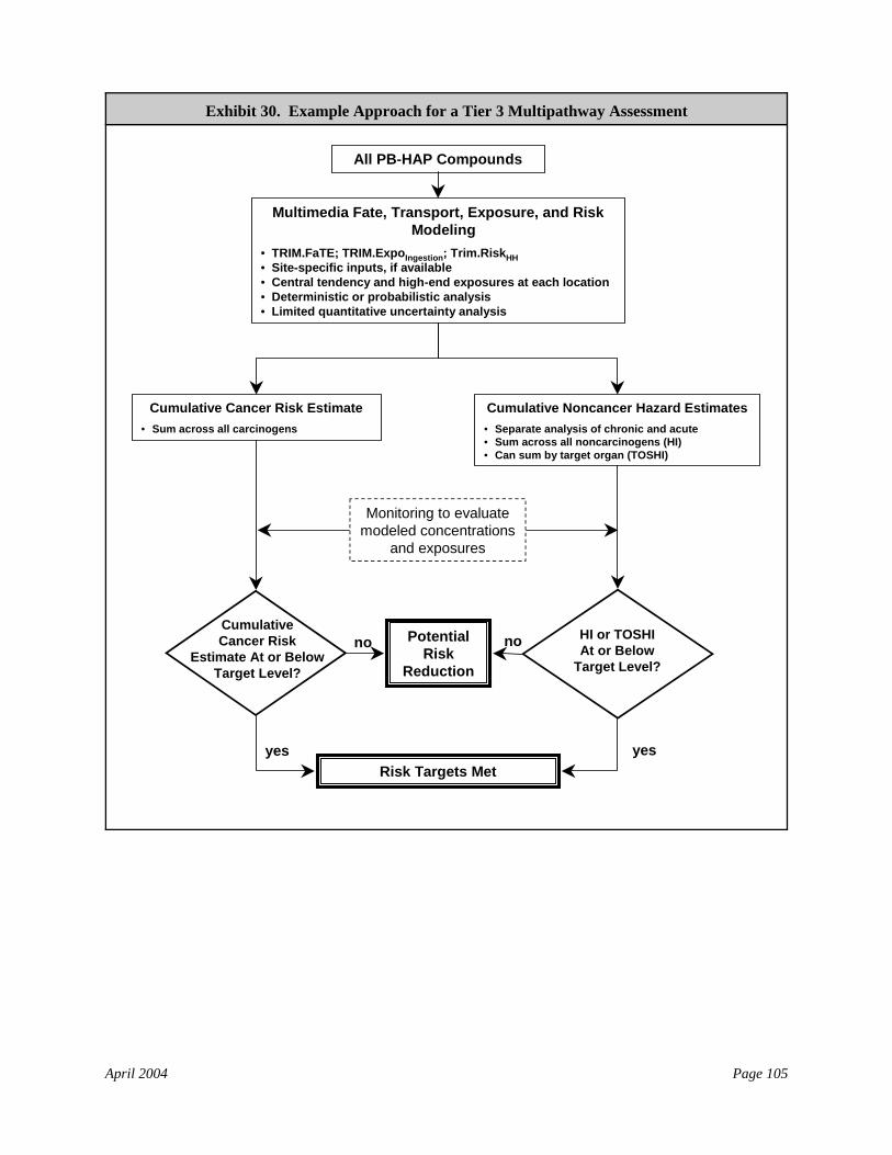
April 2004 Page 105
Multimedia Fate, Transport, Exposure, and Risk Modeling
• TRIM.FaTE; TRIM.ExpoIngestion; Trim.RiskHH• Site-specific inputs, if available• Central tendency and high-end exposures at each location• Deterministic or probabilistic analysis• Limited quantitative uncertainty analysis
Cumulative Cancer Risk Estimate• Sum across all carcinogens
Cumulative Noncancer Hazard Estimates• Separate analysis of chronic and acute• Sum across all noncarcinogens (HI)• Can sum by target organ (TOSHI)
Potential Risk
Reduction
Risk Targets Met
no no
yesyes
All PB-HAP Compounds
CumulativeCancer Risk
Estimate At or BelowTarget Level?
HI or TOSHIAt or Below
Target Level?
Monitoring to evaluate modeled concentrations
and exposures
Exhibit 30. Example Approach for a Tier 3 Multipathway Assessment
April 2004 Page 106
4.8.2 Fate and Transport Modeling
This example Tier 3 approach uses TRIM.FaTE for fate and transport modeling. Other modelscould be used. Where the assessment could support a regulatory decision, the use of analternative model commonly is agreed to in advance with the regulatory agency decision-maker.
4.8.2.1 Model Inputs
The only facility-related/source term data points required by TRIM.FaTE are chemical emissionrate, location (i.e., latitude/longitude, UTM), and emission height, all of which should beavailable from modeling performed for the inhalation risk assessment. TRIM.FaTE does all thecalculations internally for determining vapor/particle fractions and deposition rates based onchemical-specific (vs. source-specific) properties. TRIM.FaTE also requires a number of inputvariables which fall into the following general categories:
• Source, meteorological, and other input parameters;• Chemical-dependent parameters for biotic compartment types;• Chemical-dependent parameters for abiotic compartment types;• Chemical-dependent parameters independent of compartment type;• Chemical-independent parameters for biotic compartment types; and• Chemical-independent parameters for abiotic compartment types.
These variables are described in Module 16 of the TRIM.FaTE User’s Guide.(21) Note that thevalues provided with the public Reference Library are to assist users in learning how to useTRIM.FaTE and set up TRIM.FaTE scenarios. It remains each user’s responsibility to confirmor identify alternate values that are appropriate for their application and customize the library fortheir use accordingly.
4.8.2.2 Model Runs
This subsection provides an overview of what’s involved in performing a TRIM.FaTEsimulation. A more detailed description of how set up and run a TRIM.FaTE scenario isprovided in the TRIM.FaTE User’s Guide.(21) Exhibit 31 illustrates the general process forTRIM.FaTE modeling, including five general steps: (1) definition of scenario components; (2)specification of links and algorithms; (3) specification of scenario and other property values; (4)performing the simulation; and (5) analyzing results.
Definition of scenario components includes identifying the chemicals and sources to beincluded (i.e., the facility/sources and PB-HAPs), determining the modeling region, andspecifying parcels, volume elements, and compartment types. Information to assist TRIM.FaTEusers in all aspects of designing the scenario is provided in the TRIM.FaTE User’s Guide.(21) Additionally, the user will need to consider facility/source-specific information sources for eachapplication (e.g., National Land Cover Data at http://www.epa.gov/mrlc/nlcd.html - for parcelset up).
April 2004 Page 107
Define Scenario Components
• Specify chemicals and sources to be modeled
• Specify modeling region• Specify volume elements• Specify compartments• Specify simulation period
Specify Links and Algorithms
• Specify links between compartments
• Specify algorithms where required
• Specify input data for links
Specify Scenario and Other Properties
• Set initial and boundary conditions
• Specify input data (i.e., properties for all objects)
• Set simulation and output time steps
Perform Simulation
MODEL:• Updates property values for each
simulation or data time step• Calculates transfer factor for each link• Calculates moles distribution in
compartments at simulation time steps• Coverts moles to mass and concentration• Saves moles, masses, and
concentrations for output time steps
PROCESS FLOW PRIMARY TOOLS
INPUT VALUES
• Spatial data• Meteorological and other
environmental setting data• Chemical properties• Source terms and
“background” data• Data pre-processors
ALGORITHM LIBRARY
• Transfer factors
GENERAL CALCULATION TOOLS
• Differential equation solver• Partial differential equation solver
POST-PROCESSING TOOLS
• Results averagers, aggregators• Visualization tools
Analyze Results
Itera
te a
s ap
prop
riate
Exhibit 31. Developing and Executing a TRIM.FaTE Simulation
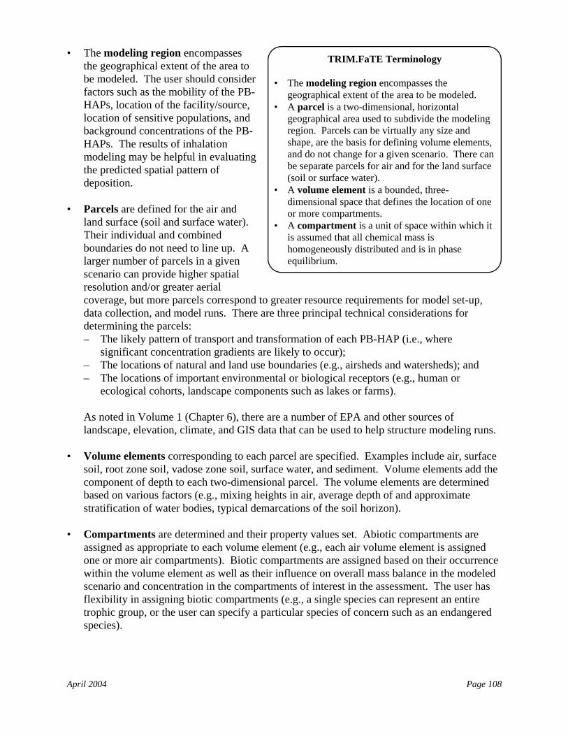
April 2004 Page 108
TRIM.FaTE Terminology
• The modeling region encompasses thegeographical extent of the area to be modeled.
• A parcel is a two-dimensional, horizontalgeographical area used to subdivide the modelingregion. Parcels can be virtually any size andshape, are the basis for defining volume elements,and do not change for a given scenario. There canbe separate parcels for air and for the land surface(soil or surface water).
• A volume element is a bounded, three-dimensional space that defines the location of oneor more compartments.
• A compartment is a unit of space within which itis assumed that all chemical mass ishomogeneously distributed and is in phaseequilibrium.
• The modeling region encompassesthe geographical extent of the area tobe modeled. The user should considerfactors such as the mobility of the PB-HAPs, location of the facility/source,location of sensitive populations, andbackground concentrations of the PB-HAPs. The results of inhalationmodeling may be helpful in evaluatingthe predicted spatial pattern ofdeposition.
• Parcels are defined for the air andland surface (soil and surface water). Their individual and combinedboundaries do not need to line up. Alarger number of parcels in a givenscenario can provide higher spatialresolution and/or greater aerialcoverage, but more parcels correspond to greater resource requirements for model set-up,data collection, and model runs. There are three principal technical considerations fordetermining the parcels:– The likely pattern of transport and transformation of each PB-HAP (i.e., where
significant concentration gradients are likely to occur);– The locations of natural and land use boundaries (e.g., airsheds and watersheds); and– The locations of important environmental or biological receptors (e.g., human or
ecological cohorts, landscape components such as lakes or farms).
As noted in Volume 1 (Chapter 6), there are a number of EPA and other sources oflandscape, elevation, climate, and GIS data that can be used to help structure modeling runs.
• Volume elements corresponding to each parcel are specified. Examples include air, surfacesoil, root zone soil, vadose zone soil, surface water, and sediment. Volume elements add thecomponent of depth to each two-dimensional parcel. The volume elements are determinedbased on various factors (e.g., mixing heights in air, average depth of and approximatestratification of water bodies, typical demarcations of the soil horizon).
• Compartments are determined and their property values set. Abiotic compartments areassigned as appropriate to each volume element (e.g., each air volume element is assignedone or more air compartments). Biotic compartments are assigned based on their occurrencewithin the volume element as well as their influence on overall mass balance in the modeledscenario and concentration in the compartments of interest in the assessment. The user hasflexibility in assigning biotic compartments (e.g., a single species can represent an entiretrophic group, or the user can specify a particular species of concern such as an endangeredspecies).
April 2004 Page 109
• The simulation period is determined. As noted with the Tier 2 analysis, this commonlyreflects the expected duration of emissions from the facility/source being evaluated. Note,however, that the rate at which a modeled chemical accumulates in all compartments slowswith time, and for chemicals that degrade there may likely be a leveling off of concentrationby 30-40 years. Therefore, the duration selected also should reflect the time necessary forthe rates of accumulation in the media/biota of interest to slow to a negligible rate of increaseor cease. If information on accumulation rate is not available, the steady-state solution maybe an acceptable output. Some additional thought is required for this option during set-up,but run time and the time needed to process results is reduced.
Specification of links and algorithms is the step in which links between compartments and sinksare specified for a given scenario. Generally, adjacent abiotic compartments are linked to eachother, and compartments at the edge of the modeling region are linked to advection sinks. Bioticcompartments generally need to be linked to the appropriate abiotic and biotic compartments. For example, each biotic compartment should be linked to all compartments that comprise itsdiet or in any way provide it a source of chemical mass and all to which it passes mass. Thesystem of links is very important, because the links provide for the assignment of the algorithmsdescribing the processes that drive chemical transfer and transformation (e.g., with the currentset of library algorithms, TRIM.FaTE cannot simulate bioconcentration in benthic invertebratesif that biotic compartment is not linked to the abiotic sediment compartment).
Specifying the scenario and other properties involves providing the remaining relevant inputvalues needed for the simulation. This involves specifying the chemical properties of each PB-HAP being modeled, any initial distribution of chemical mass in the compartments, the data foreach modeled source, environmental data needed by the selected algorithms, and the simulationand output time steps. A list of all the parameters associated with the current Reference Libraryalgorithms, which, to date, have been set to constant or time-varying numeric values (e.g., ascompared to equations or functions) is presented in Appendix D of Volume II of the TRIM.FaTETechnical Support Document (http://www.epa.gov/ttn/fera/trim_fate.html).
• Chemical-specific properties include molecular weight, melting point, half-life ordegradation rates, chemical transformation rates, and elimination rates.
• Initial and boundary conditions (e.g., initial concentrations in specific media) can bespecified.
• Source data include location, height, and emission rate.
• Environmental setting data include meteorological data (at any or various time intervals),data needed to define the characteristics of the biotic and abiotic compartments beingevaluated (e.g., soil density, current flow velocity, biomass per area, food ingestion rate), anddata needed to define properties of links between compartments (e.g., fraction of total surfacerunoff from a soil compartment to an adjacent water compartment). Collecting these datamay be difficult and time-consuming.
• The simulation time step specifies a minimum frequency at which the model will calculatetransfer factors and chemical mass exchange between (and transformed within)
April 2004 Page 110
If TRIM.ExpoIngestion is not available, riskassessors can use TRIM.FaTE to calculate PB-HAP concentrations in media and biota and thenuse the basic intake equations in the MPEmethodology to estimate exposure for eachspecific scenario evaluated.
compartments. The output time step determines the points in time at which the amount ofchemical in each compartment will be reported as output as moles, mass, or concentration.
Performing the simulation is the actual running of the model.
Analyzing results is facilitated with several TRIM.FaTE tools:
• The Averager can generate averages of TRIM.FaTE outputs in any multiple of the outputtime step as well as in monthly and annual increments. It can also limit the compartmentsincluded in the averaged file.
• The Graphical Results Viewer presents model results (moles, mass, or concentration) on amap of the parcels by using different colors to represent incremental gradients in the resultsfor a specific chemical.
• The Aggregator can produce tables in HTML, text, or comma-delimited formats thatcombine columns of output data in different ways for producing combined or comparativestatistics. Functions available for combining results include sum, average, difference, ratio,and percent difference.
4.8.3 Exposure Assessment
This example Tier 3 exposure assessmentrequires careful planning. Where theassessment could support a regulatorydecision, advance discussions with theregulatory agency risk manager areencouraged. TRIM.ExpoIngestion provides amore flexible way to assess exposurescenarios for multipathway assessments.
The initial version of TRIM.ExpoIngestion incorporates a scenario-based approach to exposureassessment. It calculates dietary intake using the output from TRIM.FaTE modeling (e.g.,concentrations) to calculate ingestion intake using the generic intake equation presented inSection 4.3 above. TRIM.ExpoIngestion currently supports 13 exposure scenarios (Exhibit 32).
Within each scenario, TRIM.ExpoIngestion provides the flexibility to incorporate a variety ofassumptions regarding exposure duration (ED), exposure frequency (EF), and varying agegroups within the ED period (e.g., an individual exposed as both a child and an adult).
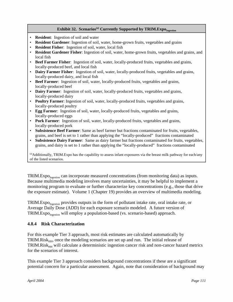
April 2004 Page 111
Exhibit 32. Scenarios(a) Currently Supported by TRIM.ExpoIngestion
• Resident: Ingestion of soil and water• Resident Gardener: Ingestion of soil, water, home-grown fruits, vegetables and grains• Resident Fisher: Ingestion of soil, water, local fish• Resident Gardener Fisher: Ingestion of soil, water, home-grown fruits, vegetables and grains, and
local fish• Beef Farmer Fisher: Ingestion of soil, water, locally-produced fruits, vegetables and grains,
locally-produced beef, and local fish• Dairy Farmer Fisher: Ingestion of soil, water, locally-produced fruits, vegetables and grains,
locally-produced dairy, and local fish• Beef Farmer: Ingestion of soil, water, locally-produced fruits, vegetables and grains,
locally-produced beef• Dairy Farmer: Ingestion of soil, water, locally-produced fruits, vegetables and grains,
locally-produced dairy• Poultry Farmer: Ingestion of soil, water, locally-produced fruits, vegetables and grains,
locally-produced poultry• Egg Farmer: Ingestion of soil, water, locally-produced fruits, vegetables and grains,
locally-produced eggs• Pork Farmer: Ingestion of soil, water, locally-produced fruits, vegetables and grains,
locally-produced pork• Subsistence Beef Farmer: Same as beef farmer but fractions contaminated for fruits, vegetables,
grains, and beef is set to 1 rather than applying the “locally-produced” fractions contaminated• Subsistence Dairy Farmer: Same as dairy farmer but fractions contaminated for fruits, vegetables,
grains, and dairy is set to 1 rather than applying the “locally-produced” fractions contaminated
(a)Additionally, TRIM.Expo has the capability to assess infant exposures via the breast milk pathway for each/anyof the listed scenarios.
TRIM.ExpoIngestion can incorporate measured concentrations (from monitoring data) as inputs. Because multimedia modeling involves many uncertainties, it may be helpful to implement amonitoring program to evaluate or further characterize key concentrations (e.g., those that drivethe exposure estimate). Volume 1 (Chapter 19) provides an overview of multimedia modeling.
TRIM.ExpoIngestion provides outputs in the form of pollutant intake rate, oral intake rate, orAverage Daily Dose (ADD) for each exposure scenario modeled. A future version ofTRIM.ExpoIngestion will employ a population-based (vs. scenario-based) approach.
4.8.4 Risk Characterization
For this example Tier 3 approach, most risk estimates are calculated automatically byTRIM.RiskHH, once the modeling scenarios are set up and run. The initial release ofTRIM.RiskHH will calculate a deterministic ingestion cancer risk and non-cancer hazard metricsfor the scenarios of interest.
This example Tier 3 approach considers background concentrations if these are a significantpotential concern for a particular assessment. Again, note that consideration of background may
April 2004 Page 112
or may not be appropriate pursuant to the specific legal and regulatory authorities under whichthe risk assessment is being conducted.
4.8.4.1 Reporting Results
The initial release of TRIM.RiskHH will provide a visualization tool for presenting analysisresults in various automated formats. The risk assessor may want to utilize this tool to assistwith development of the risk characterization summary, which generally will include thefollowing information:
• Documentation of input parameters, outputs, and risk characterization, with special emphasison the range of risk or hazard estimates;
• A simple presentation describing the assessment’s purpose and the outcome relative to thepurpose (e.g., purpose: demonstrate that risk is below target levels; outcome: low risk not demonstrated); and
• Documentation of all key assumptions or other inputs used for the assessment, such asemissions characteristics or choice of a nearby meteorological station. In particular, therationale used to define personal profiles and how they are modeled and analyzed, need to bedocumented.
4.8.4.2 Assessment and Presentation of Uncertainty
Risk managers need to understand the strengths and the limitations of the Tier 3 multipathwayrisk assessment. A critical part of the risk characterization process, therefore, is an evaluation ofthe assumptions, limitations, and uncertainties inherent in the Tier 3 assessment in order to placethe risk estimates in proper perspective.(3) Tier 3 multipathway risk assessments may bedeterministic or probabilistic and commonly include semi-quantitative sensitivity analyses andquantitative uncertainty analysis (described in Section III-5.4 above). The general quantitativeapproach to propagating or tracking uncertainty through probabilistic modeling is described inVolume 1 (Chapter 31) of this reference library.
April 2004 Page 113
This section constitutes a snapshot of EPA’s current thinking and approach to the adaptation of theevolving methods of ecological risk assessment to the context of Federal and state control of airtoxics. While inhalation risk assessment has been increasingly used in regulatory contexts over thelast several years, ecological risk assessment tools are less well developed and field tested in aregulatory context. This section should be considered a living document for review and input. Bypublishing this portion of Volume 2 in its current state of development, EPA is soliciting theinvolvement of persons with experience in this field to help improve these assessment methods foruse in a regulatory context. EPA anticipates revisions to this draft section of Volume 2 on the basisof this input.
5.0 Ecological Risk Assessment
This section describes an example approach for performing facility/source-specific ecologicalrisk assessments. In this example approach, ecological risk assessments are performed when airtoxics that persist and which also may bioaccumulate or biomagnify in food chains (e.g., the PB-HAP compounds) are present in emissions; however, other factors such as state and localregulations may need to be considered in determining whether an ecological risk assessment isappropriate for a particular facility/source. Readers unfamiliar with ecological risk assessmentare encouraged to consult the more general description of ecological risk assessment that ispresented in Part IV of Volume 1.
5.1 Introduction and Overview
The ecological risk assessment process has three main phases that correspond to the three phasesof the human health risk assessment methodology:(30)
• Planning, scoping, and problem formulation, which focuses on identifying the ecologicalrisk management goals, ecological receptors of concern, and assessment endpoints (explicitexpression of the environmental value that is to be protected, operationally defined by anecological entity and its attributes).
• Analysis includes characterization of ecological effects for the PB-HAPs present inemissions from the facility/source. A distinction is made between assessment endpoints,which are the environmental values to be protected, and measures of effects, which are thespecific metrics used to evaluate risk to the assessment endpoints. Common measures ofeffects include ecological toxicity reference values (Exhibit 33), which are discussed in moredetail in Volume 1, Chapter 25. Analysis also includes characterization of direct exposures(e.g., estimated concentrations in abiotic media) or indirect exposures (based on dietaryintake). Quantification of exposure via ingestion is similar to that for human health ingestionanalyses, except that different food items may be involved, and the appropriate ecologicalexposure factors (e.g., diet, body weight) will be different.
For this example approach, ecological effects analysis is limited to primary effects (e.g.,lethality, reduced growth, neurological/behavioral and impaired reproduction) result fromexposure of aquatic and terrestrial organisms to air toxics. An example of a chronic primary
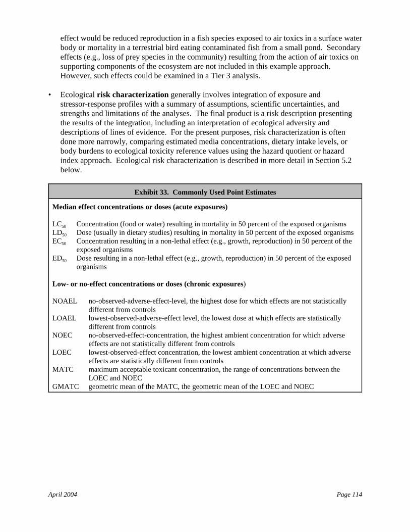
April 2004 Page 114
effect would be reduced reproduction in a fish species exposed to air toxics in a surface waterbody or mortality in a terrestrial bird eating contaminated fish from a small pond. Secondaryeffects (e.g., loss of prey species in the community) resulting from the action of air toxics onsupporting components of the ecosystem are not included in this example approach. However, such effects could be examined in a Tier 3 analysis.
• Ecological risk characterization generally involves integration of exposure andstressor-response profiles with a summary of assumptions, scientific uncertainties, andstrengths and limitations of the analyses. The final product is a risk description presentingthe results of the integration, including an interpretation of ecological adversity anddescriptions of lines of evidence. For the present purposes, risk characterization is oftendone more narrowly, comparing estimated media concentrations, dietary intake levels, orbody burdens to ecological toxicity reference values using the hazard quotient or hazardindex approach. Ecological risk characterization is described in more detail in Section 5.2below.
Exhibit 33. Commonly Used Point Estimates
Median effect concentrations or doses (acute exposures)
LC50 Concentration (food or water) resulting in mortality in 50 percent of the exposed organismsLD50 Dose (usually in dietary studies) resulting in mortality in 50 percent of the exposed organismsEC50 Concentration resulting in a non-lethal effect (e.g., growth, reproduction) in 50 percent of the
exposed organismsED50 Dose resulting in a non-lethal effect (e.g., growth, reproduction) in 50 percent of the exposed
organisms
Low- or no-effect concentrations or doses (chronic exposures)
NOAEL no-observed-adverse-effect-level, the highest dose for which effects are not statisticallydifferent from controls
LOAEL lowest-observed-adverse-effect level, the lowest dose at which effects are statisticallydifferent from controls
NOEC no-observed-effect-concentration, the highest ambient concentration for which adverseeffects are not statistically different from controls
LOEC lowest-observed-effect concentration, the lowest ambient concentration at which adverseeffects are statistically different from controls
MATC maximum acceptable toxicant concentration, the range of concentrations between theLOEC and NOEC
GMATC geometric mean of the MATC, the geometric mean of the LOEC and NOEC
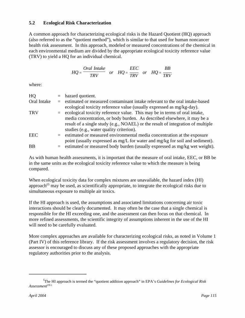
fThe HI approach is termed the “quotient addition approach” in EPA’s Guidelines for Ecological RiskAssessment(30-)
April 2004 Page 115
HQOral Intake
TRVor HQ
EECTRV
or HQBB
TRV= = =
5.2 Ecological Risk Characterization
A common approach for characterizing ecological risks is the Hazard Quotient (HQ) approach(also referred to as the “quotient method”), which is similar to that used for human noncancerhealth risk assessment. In this approach, modeled or measured concentrations of the chemical ineach environmental medium are divided by the appropriate ecological toxicity reference value(TRV) to yield a HQ for an individual chemical.
where:
HQ = hazard quotient.Oral Intake = estimated or measured contaminant intake relevant to the oral intake-based
ecological toxicity reference value (usually expressed as mg/kg-day).TRV = ecological toxicity reference value. This may be in terms of oral intake,
media concentration, or body burden. As described elsewhere, it may be aresult of a single study (e.g., NOAEL) or the result of integration of multiplestudies (e.g., water quality criterion).
EEC = estimated or measured environmental media concentration at the exposurepoint (usually expressed as mg/L for water and mg/kg for soil and sediment).
BB = estimated or measured body burden (usually expressed as mg/kg wet weight).
As with human health assessments, it is important that the measure of oral intake, EEC, or BB bein the same units as the ecological toxicity reference value to which the measure is beingcompared.
When ecological toxicity data for complex mixtures are unavailable, the hazard index (HI)approach(f) may be used, as scientifically appropriate, to integrate the ecological risks due tosimultaneous exposure to multiple air toxics.
If the HI approach is used, the assumptions and associated limitations concerning air toxicinteractions should be clearly documented. It may often be the case that a single chemical isresponsible for the HI exceeding one, and the assessment can then focus on that chemical. Inmore refined assessments, the scientific integrity of assumptions inherent in the use of the HIwill need to be carefully evaluated.
More complex approaches are available for characterizing ecological risks, as noted in Volume 1(Part IV) of this reference library. If the risk assessment involves a regulatory decision, the riskassessor is encouraged to discuss any of these proposed approaches with the appropriateregulatory authorities prior to the analysis.
April 2004 Page 116
Some Important Differences Between Ecological Risk Assessment andMultipathway Human Health Risk Assessment
• Planning and scoping. The ecological risk assessment requires more preliminary analysis anddeliberation regarding endpoints to be assessed and toxicity reference values to be used, becauseecological systems are more complex and not as well understood biologically as are human healthsystems. The planning and scoping team should include individuals with specific expertise inecological risk assessment.
• Assessment area. It may be necessary to evaluate additional portions of the assessment area thatare not of concern from a human health perspective.
• Potentially exposed populations. The focus shifts from potentially exposed groups of humans topotentially exposed populations and species of ecological receptors of concern. In many cases, theexposure assessment may need to address multiple species and life-stages, many of which havephysiological and biochemical processes that differ significantly from humans. (When threatenedor endangered species are present, the assessment may also include an evaluation of thoseorganisms as individuals).
• Exposure pathways and exposure routes. It may be necessary to assess different exposurepathways and routes that are not of concern for human health.
• Ecological effects assessment. Ecological systems have traits and properties that are differentfrom humans and, thus, the ecological effects assessment (comparable to hazard assessment forhuman health) may consider a wider range of potential causal relationships.
• Risk characterization. While risks may be assessed at multiple levels of ecological organization(i.e., organism, population, community, and ecosystem), they generally are assessed at thepopulation level in air toxics assessments. (Nevertheless, when appropriate, consideration shouldbe given to assessments as high levels of ecological organization, such as at the landscape level).
Ecological risk assessments are subject to additional sources of uncertainty and variability ascompared to multipathway human health risk assessments. In addition to the uncertaintiesassociated with multimedia modeling and sampling, the ecological risk assessment involvesmany decisions regarding choice of ecological receptors of concern and associated assessmentendpoints and measures of effects. Some of these receptors may be at levels of organizationabove individual species (e.g., communities, ecosystems), where stressor-response relationshipsare poorly defined, characterized, and/or understood (e.g., air toxics effects on loss ofcommunity prey species mentioned in Section 5.1). Because many different species and highertaxonomic groups may be included in the assessment, selection of many parameter values suchas bioconcentration factors, dose-response values, and dietary intake is more complex anduncertain for the ecological risk assessment as compared to the human health multipathway riskassessment.
April 2004 Page 117
5.3 Tier 1 Ecological Analysis
(reserved)
5.4 Tier 2 Ecological Analysis
5.4.1 Introduction
This section describes an example approach for performing a Tier 2 ecological risk assessment. Exhibit 34 provides an overview of this example approach. In this example approach, ISCST3 isused to provide deposition rates to soils and surface waters, and the MPE methodology is used toestimate PB-HAP concentrations in abiotic media (soils, surface waters, sediments) and wildlifefood items (fish) at the most impacted location. These concentrations are compared to applicableecological toxicity reference values to provide a conservative estimate of ecological risk to becalculated. If the facility/source passes this screening analysis, the risk manager can bereasonably confident that significant ecological risk is unlikely. As a consequence, monitoring isnot included explicitly in this example Tier 2 ecological analysis (although available monitoringdata can be used as inputs to the ecological exposure analysis)
5.4.2 Fate and Transport Modeling
This example approach uses the ISCST3 model for the Tier 2 fate and transport modeling.
5.4.2.1 Model Inputs
This example approach uses the same model inputs that were used for the example Tier 2 humanhealth multipathway assessment.
5.4.2.2 Model Runs
This example approach uses the same model runs that were used for the example Tier 2 humanhealth multipathway assessment.
Defining receptor locations
For this example Tier 2 analysis, terrestrial ecological receptors are assumed to occur at themodeling location (“node”) with the maximum deposition rate as determined in the example Tier2 human health multipathway assessment.
• If multiple PB-HAPs are present, the point where maximum deposition occurs for eachindividual PB-HAP may not be in the same location. This example approach assumes thatthese are all co-located (see Section 5.4.4 below).
• The point where maximum deposition occurs is used for terrestrial exposure pathways.
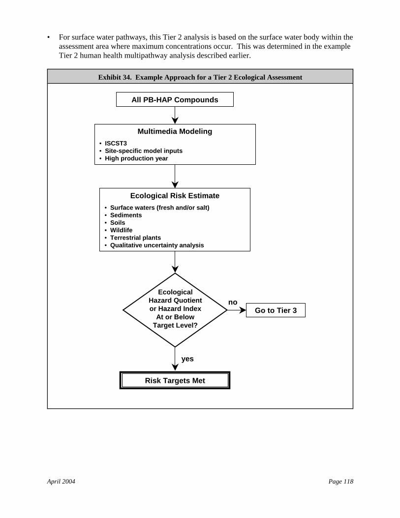
April 2004 Page 118
Multimedia Modeling• ISCST3• Site-specific model inputs• High production year
Go to Tier 3
Ecological Hazard Quotient or Hazard Index
At or BelowTarget Level?
Risk Targets Met
no
yes
Ecological Risk Estimate• Surface waters (fresh and/or salt)• Sediments• Soils• Wildlife• Terrestrial plants• Qualitative uncertainty analysis
All PB-HAP Compounds
• For surface water pathways, this Tier 2 analysis is based on the surface water body within theassessment area where maximum concentrations occur. This was determined in the exampleTier 2 human health multipathway analysis described earlier.
Exhibit 34. Example Approach for a Tier 2 Ecological Assessment
April 2004 Page 119
Defining the duration of emissions
This example approach uses the same duration of emissions that was used for the example Tier 2human health multipathway analysis.
Defining deposition/flux rates for estimating media concentrations
This example approach uses the same deposition/flux rates that were used for the example Tier 2human health multipathway analysis.
Model outputs to use
This example approach uses the same average annual deposition rates that were used for theexample Tier 2 human health multipathway analysis as inputs to the MPE methodology.
5.4.3 Exposure Assessment
5.4.3.1 Characterization of Ecological Receptors
This example Tier 2 assessment uses generic ecological receptors. In other words, modeledconcentrations of PB-HAPs in abiotic media and biota are compared to ecological toxicityreference values protective of the following groups of organisms: soil-dwelling biota, terrestrialplants, terrestrial animals, aquatic organisms, and sediment-dwelling biota. Note that EPA’sambient water quality criteria are protective of aquatic ecosystems (see Exhibit 35 below).
5.4.3.2 Defining the Point of Maximum Exposure
This example approach uses the same exposure locations used for the example Tier 2 humanhealth multipathway analysis.
• For a single PB-HAP compound, the point of maximum exposure is defined as the modeledlocation (node) at which the highest deposition rate occurs (soils) and the surface water bodywith maximum modeled concentrations.
• For multiple PB-HAP compounds, the point of maximum exposure is defined by assumingthat the point of maximum exposure occurs at the same location for each PB-HAP compound(i.e., exposure for each compound is added to calculate total exposure).
5.4.3.3 Calculation of Exposure Concentration
This example approach uses the following concentrations estimated for the example Tier 2multipathway human health assessment:
• Maximum concentrations in soil, surface water, and sediment; and• Maximum concentration in fish.
April 2004 Page 120
Note that existing monitoring data may be used to evaluate or refine the exposure estimatesbased on multimedia modeling. Volume 1 provides an overview of multimedia monitoring(Chapter 19) and additional discussion of monitoring for ecological exposure analysis (Chapter24).
5.4.3.4 Determining Intake
Ecological toxicity reference values for some PB-HAPs incorporate assumptions about wildlifeintake. For those substances, no additional calculations are required to determine intake. Forthe remaining PB-HAPs, it will be necessary to determine intake. Equations and exposurefactors used to calculate intake are found in EPA’s Wildlife Exposure Factors Handbook.(31)
5.4.4 Risk Characterization
This example approach considers three types of comparisons:
• Comparison of modeled concentrations in soils, surface waters, and sediments to ecologicaltoxicity reference values for each medium;
• Comparison of dietary intake levels for terrestrial birds and mammals to ecological toxicityreference values for wildlife ingestion; and
• Comparison of estimated body burdens in fish to ecological toxicity reference values thatrelate body burdens to adverse ecological impacts.
For these comparisons, three general types of ecological toxicity reference values are applicable(Exhibit 35):
• Toxicity reference values that relate concentrations of PB-HAPs in abiotic media (e.g., soil,sediment) to adverse effects (these may be available at the species- or community-level);
• Toxicity reference values that relate dietary intake levels of PB-HAPs to adverse effects(e.g., in birds and mammals); and
• Toxicity reference values that relate concentrations of PB-HAPs in biota (i.e., body burdens)to adverse effects in those biota. These generally have to be derived based on oral toxicitydata and assumptions about wildlife exposure factors.
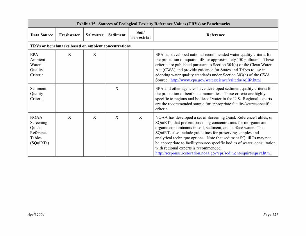
April 2004 Page 121
Exhibit 35. Sources of Ecological Toxicity Reference Values (TRVs) or Benchmarks
Data Source Freshwater Saltwater SedimentSoil/
TerrestrialReference
TRVs or benchmarks based on ambient concentrations
EPAAmbientWaterQualityCriteria
X X EPA has developed national recommended water quality criteria forthe protection of aquatic life for approximately 150 pollutants. Thesecriteria are published pursuant to Section 304(a) of the Clean WaterAct (CWA) and provide guidance for States and Tribes to use inadopting water quality standards under Section 303(c) of the CWA.Source: http://www.epa.gov/waterscience/criteria/aqlife.html
SedimentQualityCriteria
X EPA and other agencies have developed sediment quality criteria forthe protection of benthic communities. These criteria are highlyspecific to regions and bodies of water in the U.S. Regional expertsare the recommended source for appropriate facility/source-specificcriteria.
NOAAScreeningQuickReferenceTables(SQuiRTs)
X X X X NOAA has developed a set of Screening Quick Reference Tables, orSQuiRTs, that present screening concentrations for inorganic andorganic contaminants in soil, sediment, and surface water. TheSQuiRTs also include guidelines for preserving samples andanalytical technique options. Note that sediment SQuiRTs may notbe appropriate to facility/source-specific bodies of water; consultationwith regional experts is recommended.http://response.restoration.noaa.gov/cpr/sediment/squirt/squirt.html.
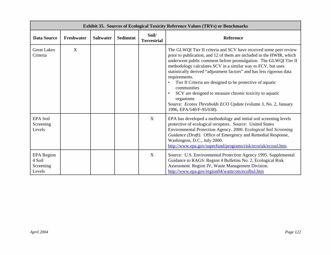
Exhibit 35. Sources of Ecological Toxicity Reference Values (TRVs) or Benchmarks
Data Source Freshwater Saltwater Sediment Soil/Terrestrial Reference
April 2004 Page 122
Great LakesCriteria
X The GLWQI Tier II criteria and SCV have received some peer reviewprior to publication, and 12 of them are included in the HWIR, whichunderwent public comment before promulgation. The GLWQI Tier IImethodology calculates SCV in a similar way to FCV, but usesstatistically derived “adjustment factors” and has less rigorous datarequirements.• Tier II Criteria are designed to be protective of aquatic
communities• SCV are designed to measure chronic toxicity to aquatic
organismsSource: Ecotox Thresholds ECO Update (volume 3, No. 2, January1996, EPA/540/F-95/038).
EPA SoilScreeningLevels
X EPA has developed a methodology and initial soil screening levelsprotective of ecological receptors. Source: United StatesEnvironmental Protection Agency. 2000. Ecological Soil ScreeningGuidance (Draft). Office of Emergency and Remedial Response,Washington, D.C., July 2000. http://www.epa.gov/superfund/programs/risk/ecorisk/ecossl.htm.
EPA Region4 SoilScreeningLevels
X Source: U.S. Environmental Protection Agency 1995. SupplementalGuidance to RAGS: Region 4 Bulletins No. 2. Ecological RiskAssessment. Region IV, Waste Management Division. http://www.epa.gov/region04/waste/ots/ecolbul.htm
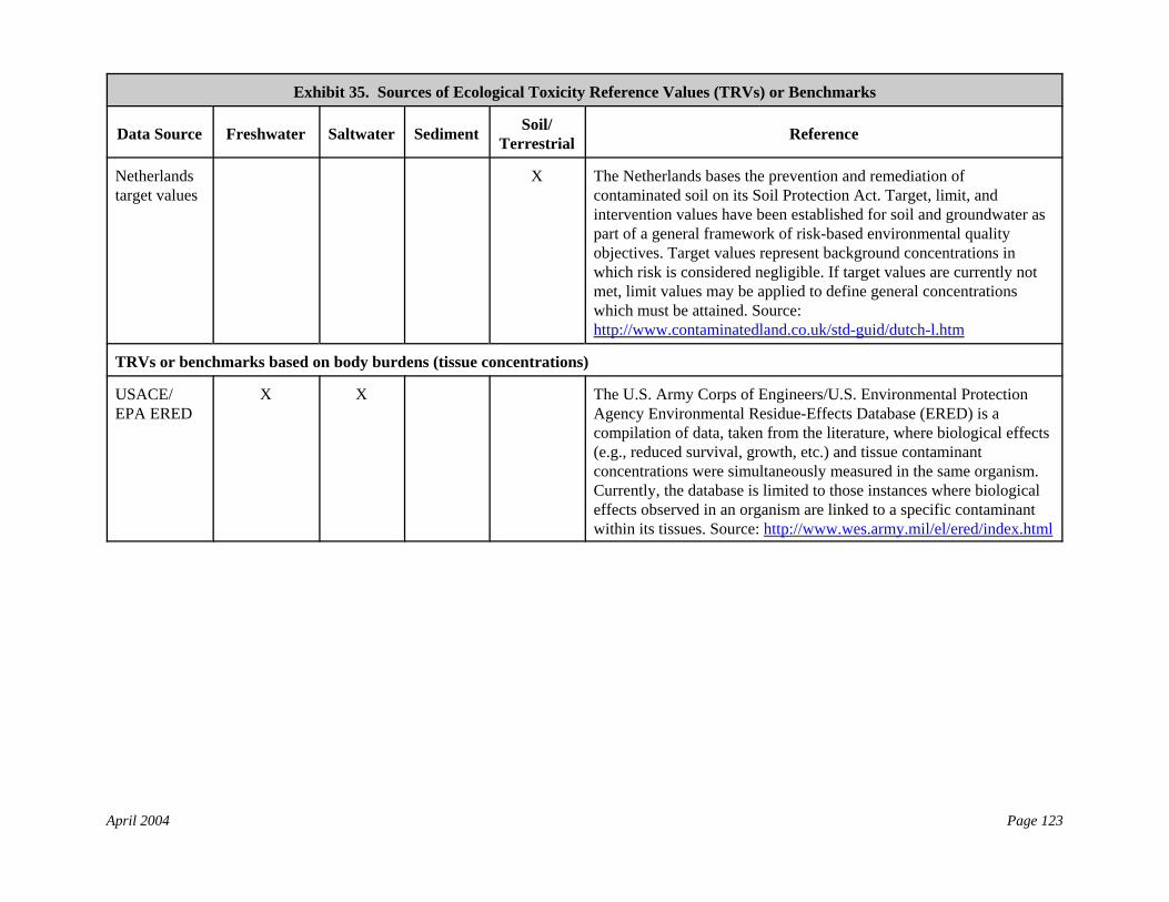
Exhibit 35. Sources of Ecological Toxicity Reference Values (TRVs) or Benchmarks
Data Source Freshwater Saltwater Sediment Soil/Terrestrial Reference
April 2004 Page 123
Netherlandstarget values
X The Netherlands bases the prevention and remediation ofcontaminated soil on its Soil Protection Act. Target, limit, andintervention values have been established for soil and groundwater aspart of a general framework of risk-based environmental qualityobjectives. Target values represent background concentrations inwhich risk is considered negligible. If target values are currently notmet, limit values may be applied to define general concentrationswhich must be attained. Source: http://www.contaminatedland.co.uk/std-guid/dutch-l.htm
TRVs or benchmarks based on body burdens (tissue concentrations)
USACE/EPA ERED
X X The U.S. Army Corps of Engineers/U.S. Environmental ProtectionAgency Environmental Residue-Effects Database (ERED) is acompilation of data, taken from the literature, where biological effects(e.g., reduced survival, growth, etc.) and tissue contaminantconcentrations were simultaneously measured in the same organism.Currently, the database is limited to those instances where biologicaleffects observed in an organism are linked to a specific contaminantwithin its tissues. Source: http://www.wes.army.mil/el/ered/index.html
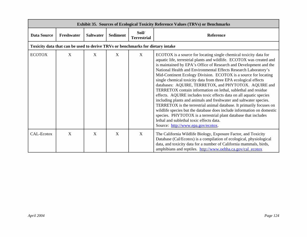
Exhibit 35. Sources of Ecological Toxicity Reference Values (TRVs) or Benchmarks
Data Source Freshwater Saltwater Sediment Soil/Terrestrial Reference
April 2004 Page 124
Toxicity data that can be used to derive TRVs or benchmarks for dietary intake
ECOTOX X X X X ECOTOX is a source for locating single chemical toxicity data foraquatic life, terrestrial plants and wildlife. ECOTOX was created andis maintained by EPA’s Office of Research and Development and theNational Health and Environmental Effects Research Laboratory’sMid-Continent Ecology Division. ECOTOX is a source for locatingsingle chemical toxicity data from three EPA ecological effectsdatabases: AQUIRE, TERRETOX, and PHYTOTOX. AQUIRE andTERRETOX contain information on lethal, sublethal and residueeffects. AQUIRE includes toxic effects data on all aquatic speciesincluding plants and animals and freshwater and saltwater species. TERRETOX is the terrestrial animal database. It primarily focuses onwildlife species but the database does include information on domesticspecies. PHYTOTOX is a terrestrial plant database that includeslethal and sublethal toxic effects data.Source: http://www.epa.gov/ecotox.
CAL-Ecotox X X X X The California Wildlife Biology, Exposure Factor, and ToxicityDatabase (Cal/Ecotox) is a compilation of ecological, physiologicaldata, and toxicity data for a number of California mammals, birds,amphibians and reptiles. http://www.oehha.ca.gov/cal_ecotox
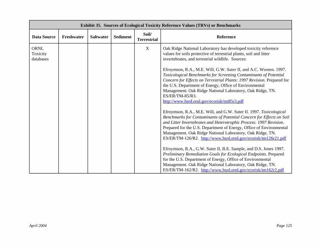
Exhibit 35. Sources of Ecological Toxicity Reference Values (TRVs) or Benchmarks
Data Source Freshwater Saltwater Sediment Soil/Terrestrial Reference
April 2004 Page 125
ORNLToxicitydatabases
X Oak Ridge National Laboratory has developed toxicity referencevalues for soils protective of terrestrial plants, soil and litterinvertebrates, and terrestrial wildlife. Sources:
Efroymson, R.A., M.E. Will, G.W. Suter II, and A.C. Wooten. 1997.Toxicological Benchmarks for Screening Contaminants of PotentialConcern for Effects on Terrestrial Plants: 1997 Revision. Prepared forthe U.S. Department of Energy, Office of EnvironmentalManagement. Oak Ridge National Laboratory, Oak Ridge, TN.ES/ER/TM-85/R3. http://www.hsrd.ornl.gov/ecorisk/tm85r3.pdf
Efroymson, R.A., M.E. Will, and G.W. Suter II. 1997. ToxicologicalBenchmarks for Contaminants of Potential Concern for Effects on Soiland Litter Invertebrates and Heterotrophic Process: 1997 Revision.Prepared for the U.S. Department of Energy, Office of EnvironmentalManagement. Oak Ridge National Laboratory, Oak Ridge, TN.ES/ER/TM-126/R2. http://www.hsrd.ornl.gov/ecorisk/tm126r21.pdf
Efroymson, R.A., G.W. Suter II, B.E. Sample, and D.S. Jones 1997.Preliminary Remediation Goals for Ecological Endpoints. Preparedfor the U.S. Department of Energy, Office of EnvironmentalManagement. Oak Ridge National Laboratory, Oak Ridge, TN.ES/ER/TM-162/R2. http://www.hsrd.ornl.gov/ecorisk/tm162r2.pdf
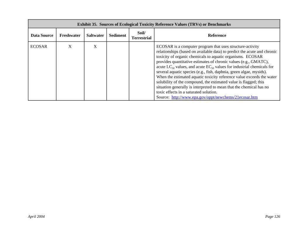
Exhibit 35. Sources of Ecological Toxicity Reference Values (TRVs) or Benchmarks
Data Source Freshwater Saltwater Sediment Soil/Terrestrial Reference
April 2004 Page 126
ECOSAR X X ECOSAR is a computer program that uses structure-activityrelationships (based on available data) to predict the acute and chronictoxicity of organic chemicals to aquatic organisms. ECOSARprovides quantitative estimates of chronic values (e.g., GMATC),acute LC50 values, and acute EC50 values for industrial chemicals forseveral aquatic species (e.g., fish, daphnia, green algae, mysids). When the estimated aquatic toxicity reference value exceeds the watersolubility of the compound, the estimated value is flagged; thissituation generally is interpreted to mean that the chemical has notoxic effects in a saturated solution.Source: http://www.epa.gov/oppt/newchems/21ecosar.htm
April 2004 Page 127
5.4.4.1 Reporting Results
For this example approach, a relative simple summary can be used to report results, as long as itis consistent with the need to make the results both transparent and reproducible. The summarygenerally will include the following information:
• Documentation of input parameters, output values, and risk characterization, with specialemphasis on comparing estimated risk/hazard to risk targets;
• A simple presentation describing the assessment’s purpose (e.g., to determine whether risk isbelow levels of concern) and the outcome relative to that purpose (e.g., low risk is notdemonstrated); and
• Documentation of anything that is discretionary (i.e., anything that is facility-specific), suchas emissions characteristics or choice of a meteorological station other than the nearest.
5.4.4.2 Assessment and Presentation of Uncertainty
Risk managers need to understand the strengths and the limitations of the Tier 2 ecological riskassessment. A critical part of the risk characterization process, therefore, is an evaluation of theassumptions, limitations, and uncertainties inherent in the Tier 2 assessment in order to place therisk estimates in proper perspective.(3) Tier 2 ecological assessments commonly include aquantitative or qualitative description of the uncertainty for each parameter and indicating thepossible influence of these uncertainties on the final risk estimates given knowledge of themodels used. Tier 2 assessments also may include a semi-quantitative sensitivity analyses. These approaches are described in Section III-5.4 above. Sensitivity analyses are discussed inmore detail in Volume 1 (Chapters 3 and 13) of this reference library.
April 2004 Page 128
5.5 Tier 3 Ecological Analysis
5.5.1 Introduction
This section describes an example approach for performing a Tier 3 ecological risk assessment. Exhibit 36 provides an overview of this example approach. This example Tier 3 assessment issignificantly different than the Tier 2 example approach, in that it involves the use ofTRIM.FaTE for multimedia modeling, specific consideration of ecological receptor locations,and use of a risk model (TRIM.RiskEco) to provide a more refined characterization of risk,including multiple estimates of risk.
This example Tier 3 analysis allows considerable flexibility in analytical approach and detail.
• In this example approach, TRIM.FaTE is used for multimedia modeling and generatesconcentrations in abiotic media, body burdens, and wildlife intake rates that feed directly intoTRIM.RiskEco for ecological risk characterization. TRIM.FaTE allows considerable spatialrefinement in selecting exposure locations, and provides concentrations for user-specified(actual) locations.
• In this example approach, a risk model (TRIM.RiskEco) is used to characterize ecological risk. This module performs ecological risk characterization calculations for multimedia ecologicalrisk assessments of toxic air pollutants or other chemical contaminants. The output ofTRIM.RiskEco are hazard quotients (HQ) that can be processed with TRIM.Risk analysistools to prepare tables and charts that can be used in communicating the risk assessmentresults.
• In this example approach, monitoring data are used to evaluate or further characterize keyconcentration data.
Exhibit 37 illustrates how the TRIM modules and data correspond to EPA’s ecological riskassessment framework as described in the Framework for Ecological Risk Assessment.(32) Guidance for how to structure TRIM analyses for ecological risk assessment is provided in theTRIM.RiskEco User’s Guide.(33) This example Tier 3 analysis will be highly facility/source-specific and will require careful planning.
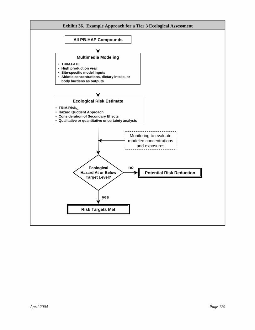
April 2004 Page 129
Multimedia Modeling• TRIM.FaTE• High production year• Site-specific model inputs• Abiotic concentrations, dietary intake, or
body burdens as outputs
Potential Risk ReductionEcological
Hazard At or BelowTarget Level?
Risk Targets Met
no
yes
Ecological Risk Estimate• TRIM.RiskEco• Hazard Quotient Approach• Consideration of Secondary Effects• Qualitative or quantitative uncertainty analysis
All PB-HAP Compounds
Monitoring to evaluate modeled concentrations
and exposures
Exhibit 36. Example Approach for a Tier 3 Ecological Assessment
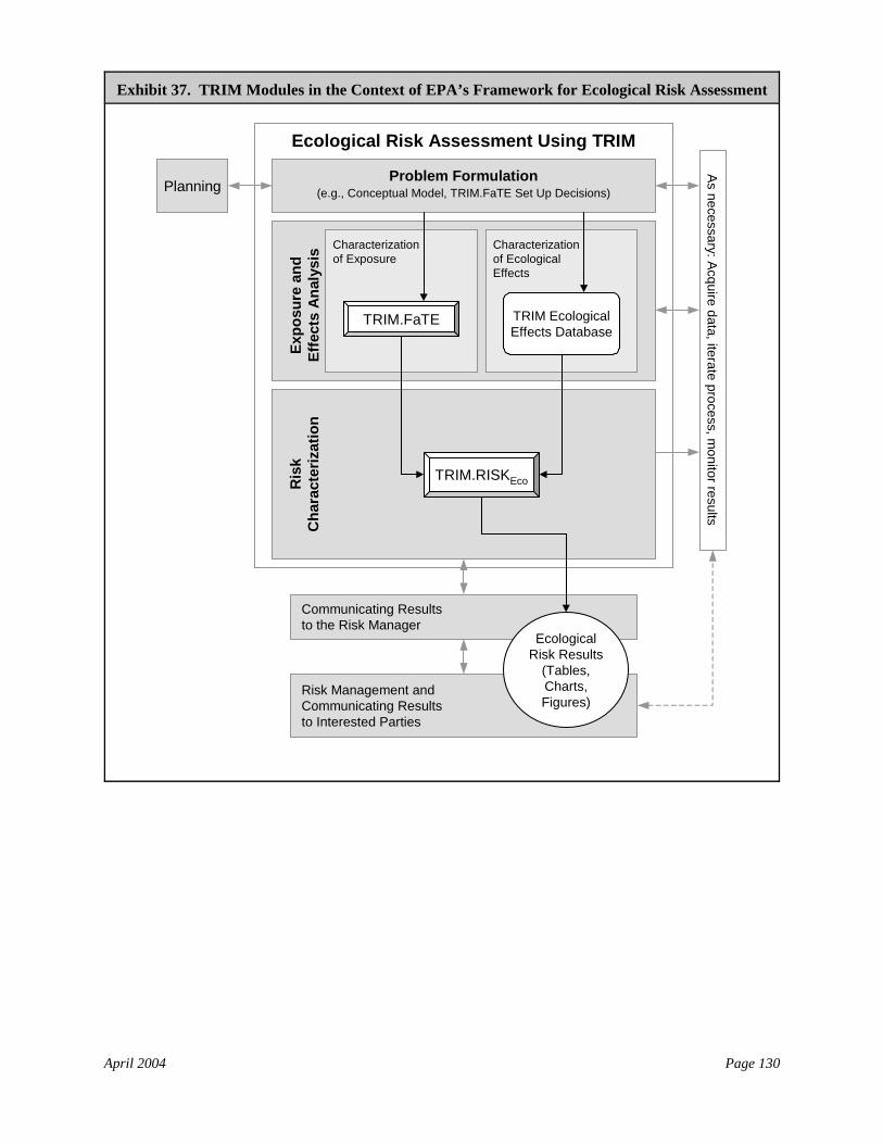
April 2004 Page 130
Ecological Risk Assessment Using TRIM
Problem Formulation(e.g., Conceptual Model, TRIM.FaTE Set Up Decisions)
Expo
sure
and
Ef
fect
s A
naly
sis
PlanningA
s necessary: Acquire data, iterate process, monitor results
Communicating Resultsto the Risk Manager
Risk Management andCommunicating Resultsto Interested Parties
TRIM.RISKEco
Ecological Risk Results
(Tables, Charts, Figures)
Ris
k C
hara
cter
izat
ion
Characterizationof Exposure
Characterizationof EcologicalEffects
TRIM Ecological Effects Database
TRIM.FaTE
Exhibit 37. TRIM Modules in the Context of EPA’s Framework for Ecological Risk Assessment
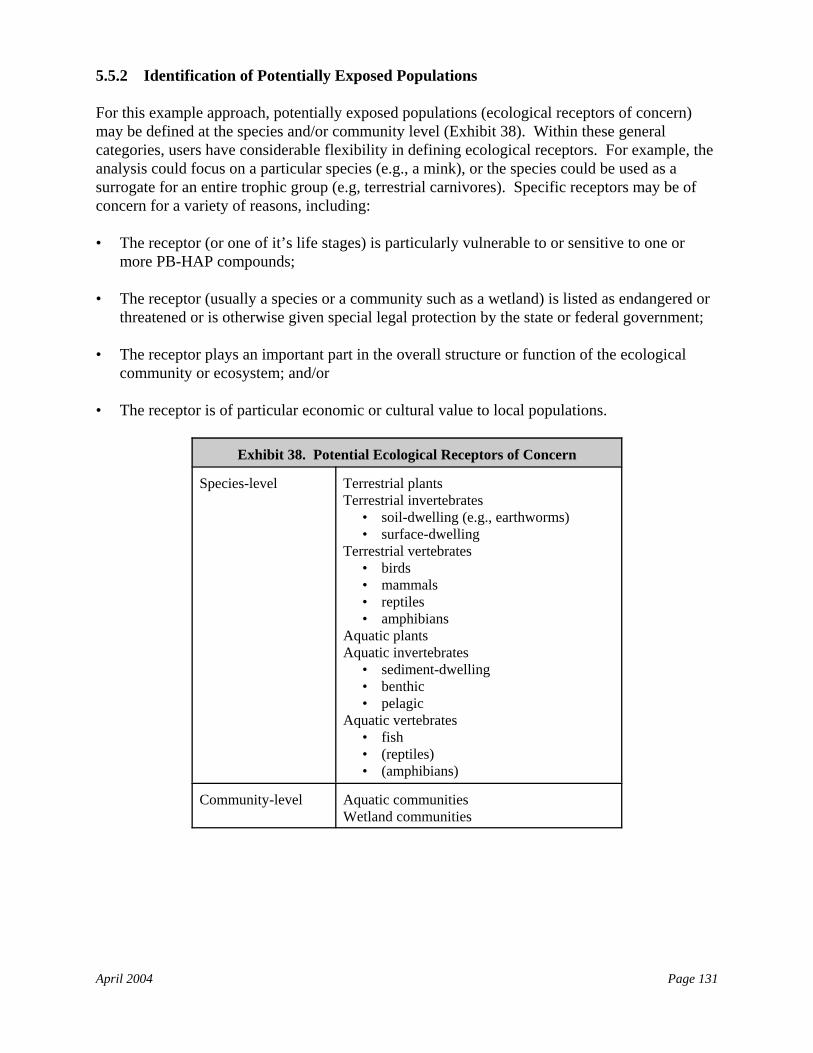
April 2004 Page 131
5.5.2 Identification of Potentially Exposed Populations
For this example approach, potentially exposed populations (ecological receptors of concern)may be defined at the species and/or community level (Exhibit 38). Within these generalcategories, users have considerable flexibility in defining ecological receptors. For example, theanalysis could focus on a particular species (e.g., a mink), or the species could be used as asurrogate for an entire trophic group (e.g, terrestrial carnivores). Specific receptors may be ofconcern for a variety of reasons, including:
• The receptor (or one of it’s life stages) is particularly vulnerable to or sensitive to one ormore PB-HAP compounds;
• The receptor (usually a species or a community such as a wetland) is listed as endangered orthreatened or is otherwise given special legal protection by the state or federal government;
• The receptor plays an important part in the overall structure or function of the ecologicalcommunity or ecosystem; and/or
• The receptor is of particular economic or cultural value to local populations.
Exhibit 38. Potential Ecological Receptors of Concern
Species-level Terrestrial plantsTerrestrial invertebrates
• soil-dwelling (e.g., earthworms)• surface-dwelling
Terrestrial vertebrates• birds• mammals• reptiles• amphibians
Aquatic plantsAquatic invertebrates
• sediment-dwelling• benthic• pelagic
Aquatic vertebrates• fish• (reptiles)• (amphibians)
Community-level Aquatic communitiesWetland communities
April 2004 Page 132
Often it is important to understand the aquatic and terrestrial food webs in the habitats ofconcern, because these can be important parts of ecological exposure pathways. Top predatorsare often of special concern for exposure to PB-HAP compounds.
For this example approach, ecological receptors for each habitat potentially impacted areidentified to ensure (1) plant and animal communities representative of the habitat arerepresented by the habitat-specific food web, and (2) potentially complete exposure pathways areidentified. Ecological receptor identification may need to include species both known andexpected to be present in a specific habitat being evaluated, and include resident and migratorypopulations. Consultation with ecological experts is encouraged (see Volume 1, Chapter 23).
5.5.3 Assessment Endpoints and Measures of Effect
As discussed in Volume 1 of this reference library (Chapter 23), an assessment endpoint is anexplicit expression of the “actual environmental value that is to be protected” or is of concern. Itincludes the identification of the ecological entity for the analysis (e.g., a species, ecologicalresource, habitat type, or community) as well as the attribute of that entity that is potentially atrisk (e.g., reproductive success, production per unit area, surface area coverage, biodiversity) andthat is important to protect. Measures of effects are the metrics by which these endpoints areassessed.(30) EPA has recently released guidance that describes a set of endpoints, known asGeneric Ecological Assessment Endpoints (GEAE), that can be considered and adapted forspecific ecological risk assessments (Exhibit 39).(34)
Where ecological effects information is available, TRIM.RiskEco allows the user to select (orinput) multiple measures of effects for a given ecological receptor. For example, differenttoxicity reference values (TRVs) may be available for the same species that are associated withdifferent measures of effects (e.g., reproductive effects, respiration, mortality). Volume 1(Chapter 25) provides a discussion on the selection of TRVs for a particular assessment.
Where available ecological toxicity reference values do not consider secondary effects (e.g., oncommunities), it may be possible to use TRIM.RiskEco outputs as a starting point for evaluatingsecondary effects, either qualitatively or quantitatively. For this example Tier 3 assessment, riskassessors are encouraged to include secondary effects as assessment endpoints to the extent thatresources and information allows.
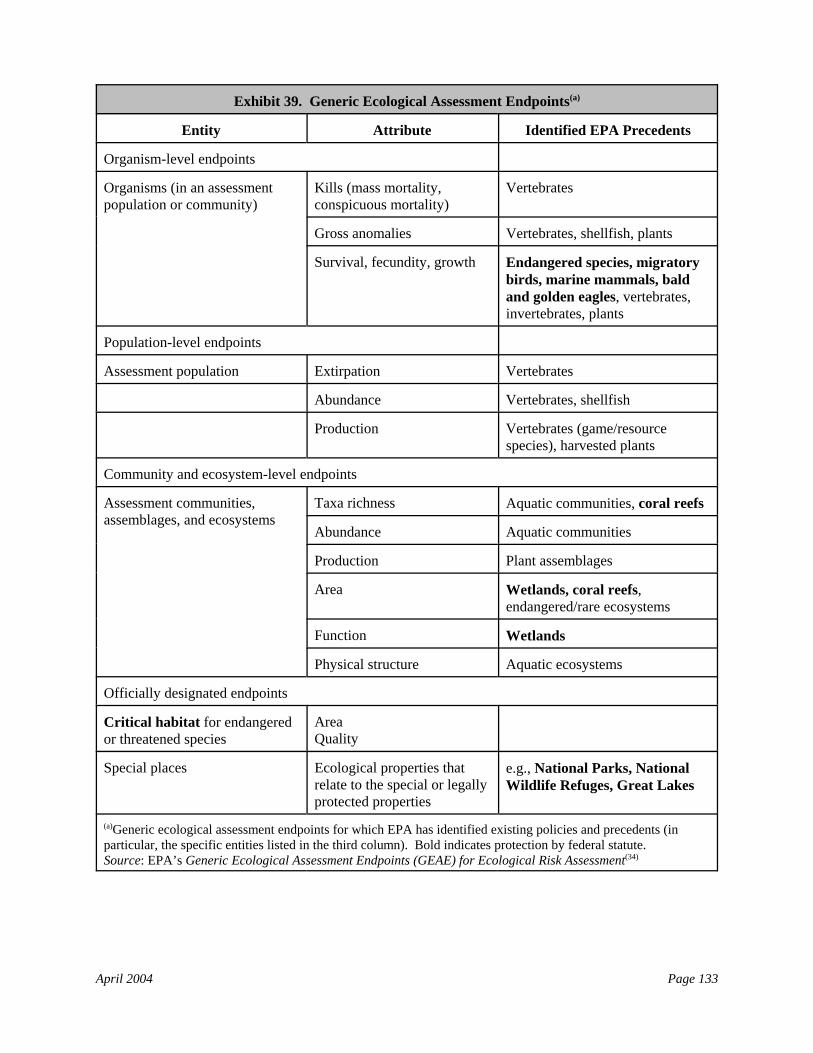
April 2004 Page 133
Exhibit 39. Generic Ecological Assessment Endpoints(a)
Entity Attribute Identified EPA Precedents
Organism-level endpoints
Organisms (in an assessmentpopulation or community)
Kills (mass mortality,conspicuous mortality)
Vertebrates
Gross anomalies Vertebrates, shellfish, plants
Survival, fecundity, growth Endangered species, migratorybirds, marine mammals, baldand golden eagles, vertebrates,invertebrates, plants
Population-level endpoints
Assessment population Extirpation Vertebrates
Abundance Vertebrates, shellfish
Production Vertebrates (game/resourcespecies), harvested plants
Community and ecosystem-level endpoints
Assessment communities,assemblages, and ecosystems
Taxa richness Aquatic communities, coral reefs
Abundance Aquatic communities
Production Plant assemblages
Area Wetlands, coral reefs,endangered/rare ecosystems
Function Wetlands
Physical structure Aquatic ecosystems
Officially designated endpoints
Critical habitat for endangeredor threatened species
AreaQuality
Special places Ecological properties thatrelate to the special or legallyprotected properties
e.g., National Parks, NationalWildlife Refuges, Great Lakes
(a)Generic ecological assessment endpoints for which EPA has identified existing policies and precedents (inparticular, the specific entities listed in the third column). Bold indicates protection by federal statute.Source: EPA’s Generic Ecological Assessment Endpoints (GEAE) for Ecological Risk Assessment(34)
April 2004 Page 134
5.5.4 Fate and Transport Modeling
This subsection provides an overview of TRIM.FaTE set up and execution. This is explainedmore fully in section 4.8.2 and in the TRIM.FaTE User’s Guide.(21)
• The modeling region encompasses all areas where ecological receptors are known or likelyto occur, especially any important receptors such as wetlands, endangered/threatened species,or areas that are particularly important to regional populations (e.g., wintering areas,migration routes, breeding grounds).
• Parcels are defined to adequately provide an assessment of exposures at the locations wherethe ecological receptors identified above occur.
• Volume elements are defined to include all potential routes of ecological exposure (e.g., rootzone soil for earthworms).
• Compartments can be defined in a flexible manner depending on the level of detail in whichecological receptors are characterized for the analysis. For example, a single species (e.g.,lake trout) could be used as a surrogate for all higher-trophic level fish, or the analysis couldidentify several multiple species of higher-trophic level fish.
• Links and algorithms should incorporate the processes that drive chemical transfer andtransformation that are relevant to the ecological exposure assessment.
• As noted above, the TRIM.FaTE model runs may be set up and performed along with theTier 3 human health model runs.
• Results can be processed with TRIM.Risk analysis or other tools to prepare tables and chartsthat can be used in communicating the risk assessment results.
5.5.5 Exposure Assessment
TRIM.FaTE provides three general metrics of ecological exposure (Exhibit 40): ambientconcentrations in abotic media, ingestion intake levels for specified receptors, and body burdens.Each of these can be compared with a corresponding ecological toxicity reference value for riskcharacterization. Intake and body burdens are calculated for specific ecological receptorsspecified in the model setup, although these receptors may be matched with TRVs for surrogates,as appropriate, in TRIM.RiskEco.
The user can specify the specific time points of interest of the TRIM.FaTE exposure simulationto be compared with each type of ecological toxicity reference values.
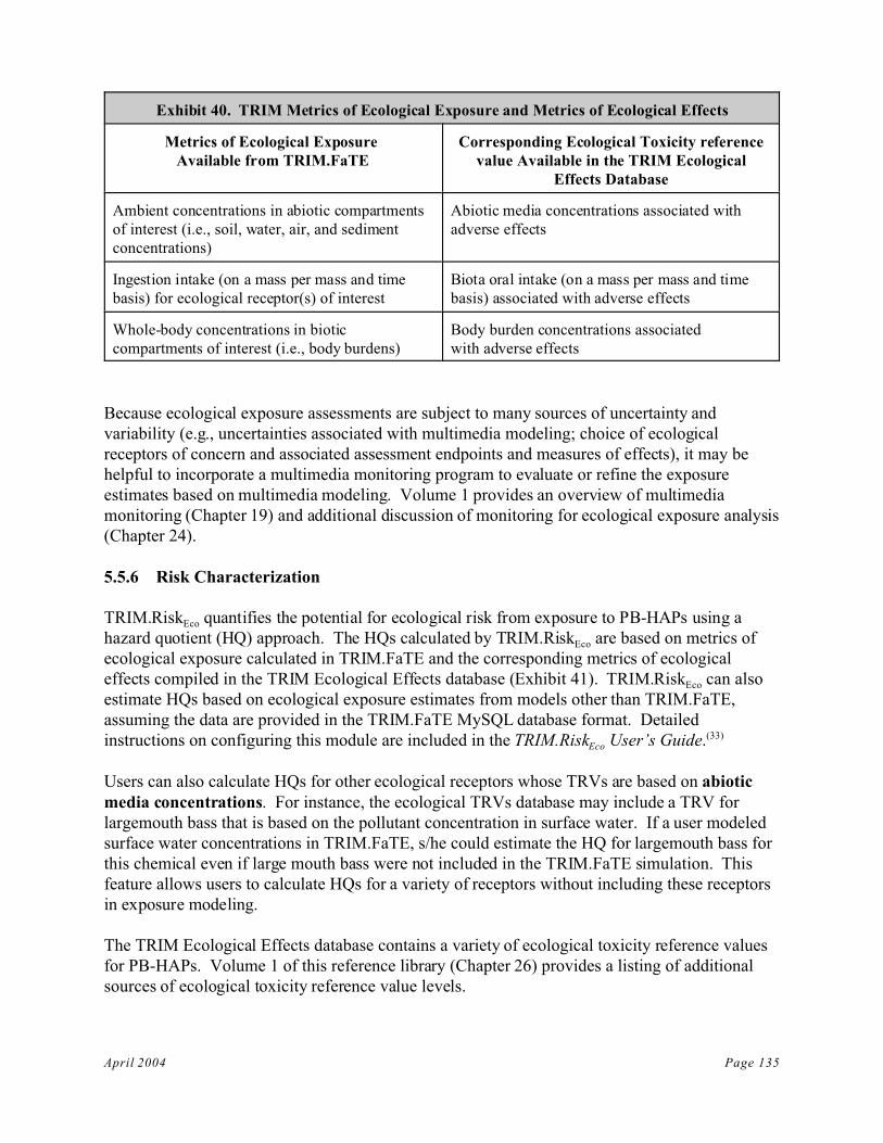
April 2004 Page 135
Exhibit 40. TRIM Metrics of Ecological Exposure and Metrics of Ecological Effects
Metrics of Ecological Exposure Available from TRIM.FaTE
Corresponding Ecological Toxicity referencevalue Available in the TRIM Ecological
Effects Database
Ambient concentrations in abiotic compartmentsof interest (i.e., soil, water, air, and sedimentconcentrations)
Abiotic media concentrations associated withadverse effects
Ingestion intake (on a mass per mass and timebasis) for ecological receptor(s) of interest
Biota oral intake (on a mass per mass and timebasis) associated with adverse effects
Whole-body concentrations in bioticcompartments of interest (i.e., body burdens)
Body burden concentrations associatedwith adverse effects
Because ecological exposure assessments are subject to many sources of uncertainty andvariability (e.g., uncertainties associated with multimedia modeling; choice of ecologicalreceptors of concern and associated assessment endpoints and measures of effects), it may behelpful to incorporate a multimedia monitoring program to evaluate or refine the exposureestimates based on multimedia modeling. Volume 1 provides an overview of multimediamonitoring (Chapter 19) and additional discussion of monitoring for ecological exposure analysis(Chapter 24).
5.5.6 Risk Characterization
TRIM.RiskEco quantifies the potential for ecological risk from exposure to PB-HAPs using ahazard quotient (HQ) approach. The HQs calculated by TRIM.RiskEco are based on metrics ofecological exposure calculated in TRIM.FaTE and the corresponding metrics of ecologicaleffects compiled in the TRIM Ecological Effects database (Exhibit 41). TRIM.RiskEco can alsoestimate HQs based on ecological exposure estimates from models other than TRIM.FaTE,assuming the data are provided in the TRIM.FaTE MySQL database format. Detailedinstructions on configuring this module are included in the TRIM.RiskEco User’s Guide.(33)
Users can also calculate HQs for other ecological receptors whose TRVs are based on abioticmedia concentrations. For instance, the ecological TRVs database may include a TRV forlargemouth bass that is based on the pollutant concentration in surface water. If a user modeledsurface water concentrations in TRIM.FaTE, s/he could estimate the HQ for largemouth bass forthis chemical even if large mouth bass were not included in the TRIM.FaTE simulation. Thisfeature allows users to calculate HQs for a variety of receptors without including these receptorsin exposure modeling.
The TRIM Ecological Effects database contains a variety of ecological toxicity reference valuesfor PB-HAPs. Volume 1 of this reference library (Chapter 26) provides a listing of additionalsources of ecological toxicity reference value levels.
April 2004 Page 136
5.5.6.1 Reporting Results
TRIM.Risk provides a visualization tool for presenting analysis results in various automatedformats. The risk assessor may want to utilize this tool to assist with development of the riskcharacterization summary, which generally will include the following information:
• Documentation of input parameters, outputs, and risk characterization, with special emphasison the range of risk or hazard estimates;
• A simple presentation describing the assessment’s purpose and the outcome relative to thepurpose (e.g., purpose: demonstrate that risk is below target levels; outcome: low risk notdemonstrated); and
• Documentation of all key assumptions or other inputs used for the assessment, such asemissions characteristics or choice of a nearby meteorological station.
5.5.6.2 Assessment and Presentation of Uncertainty
Risk managers need to understand the strengths and the limitations of the Tier 3 ecological riskassessment. A critical part of the risk characterization process, therefore, is an evaluation of theassumptions, limitations, and uncertainties inherent in the Tier 3 assessment in order to place therisk estimates in proper perspective.(3) Tier 3 ecological risk assessments may be deterministic orprobabilistic and commonly include semi-quantitative sensitivity analyses and quantitativeuncertainty analysis (described in Section III-5.4 above). The general quantitative approach topropagating or tracking uncertainty through probabilistic modeling is described in Volume 1(Chapter 31) of this reference library.
April 2004 Page 137
1. U.S. Environmental Protection Agency. 2003. Framework for Cumulative Risk Assessment. Risk Assessment Forum, Washington, DC 20460, May 2003, EPA/630/P-02/001F; availableat http://cfpub.epa.gov/ncea/raf/recordisplay.cfm?deid=54944.
2. U.S. Environmental Protection Agency. 1999. Residual Risk Report to Congress. Office ofAir Quality Planning and Standards, Research Triangle Park, NC 27711, March 1999, EPA-453/R-99-001; available at http://www.epa.gov/ttn/oarpg/t3/reports/risk_rep.pdf.
3. U.S. Environmental Protection Agency. 1995. Policy for Risk Characterization at the U.S.Environmental Protection Agency. Science Policy Council, Washington, D.C., March 1995,available at: http://64.2.134.196/committees/aqph/rcpolicy.pdf.
4. Hattis. D.B. and D.E. Burmaster. 1994. Assessment of variability and uncertaintydistributions for practical risk analyses. Risk Analysis 14(5):713-730.
U.S. Environmental Protection Agency. 1999. Report of the Workshop on Selecting InputDistributions for Probabilistic Assessments. Risk Assessment Forum, Washington, DC.EPA/630/R-98/004.
U.S. Environmental Protection Agency. 1997. Guiding Principles for Monte Carlo Analysis.Risk Assessment Forum, Washington, DC. March 1997. EPA-630/R-97-001; available athttp://www.epa.gov/NCEA/pdfs/montcarl.pdf.
U.S. Environmental Protection Agency. 1988. National Emission Standards for HazardousAir Pollutants. Federal Register 53(145):28496-28056, Proposed Rule and Notice of PublicHearing, July 28, 1988.
Finkel, A.M. 1990. Confronting Uncertainty in Risk Management: A Guide for Decision-Makers. Center for Risk Management, Resources for the Future. Washington, DC.
U.S. Environmental Protection Agency. 1997. Policy for Use of Probabilistic Analysis inRisk Assessment. Office of the Administrator, Washington, DC. May 15, 1997; available athttp://www.epa.gov/osp/spc/probpol.htm.
National Council on Radiation Protection and Measurements. 1996. A Guide for UncertaintyAnalysis in Dose and Risk Assessments Related to Environmental Contamination. NCRPCommentary No. 14; available at http://www.ncrp.com/comm14.html.
5. U.S. Environmental Protection Agency. 2001. Risk Assessment Guidance for Superfund(RAGS). Volume III - Part A. Process for Conducting Probabilistic Risk Assessment. Officeof Emergency and Remedial Response, Washington, D.C.(http://www.epa.gov/superfund/programs/risk/rags3a/index.htm).
References (note that some numbered references include multiple citations)
April 2004 Page 138
6. U.S. Environmental Protection Agency. 1992. Screening Procedures for Estimating the AirQuality Impact of Stationary Sources, Revised. Office of Air Quality Planning and Standards,Research Triangle Park, North Carolina, October 1992. EPA-454/R-92-019. Available at:http://www.epa.gov/scram001/tt25.htm#guidance.
7. U.S. Environmental Protection Agency. 2002. User’s Guide for the Human Exposure Model(HEM). Office of Air Quality Planning and Standards, Research Triangle Park, NC; currentversion available at: http://www.epa.gov/ttn/fera/human_hem.html.
8. U.S. Environmental Protection Agency. 1995. SCREEN3 Model Users’ Guide. Office ofAir Quality Planning and Standards, Research Triangle Park, NC. EPA-454/B-95-004. (http://www.epa.gov/scram001/userg/screen/screen3d.pdf).
9. U.S. Environmental Protection Agency. 1995. User’s Guide for the Industrial SourceComplex (ISC3) Dispersion Models Volume I - User’s Instructions. Office of Air QualityPlanning and Standards, Research Triangle Park, NC. September 1995. EPA-454/B-95-0031; available at http://www.epa.gov/scram001/tt22.htm#isc.
10. U.S. Environmental Protection Agency. 2003. Total Risk Integrated MethodologyTrim.ExpoInhalation User’s Document. Volume 1: Air Pollutants Exposure Model (APEX,Version 3) User’s Guide. Office of Air Quality Planning and Standards, Research TrianglePark, NC. April 2003.
11. EPA’s carcinogen risk assessment guidelines were first published in 1986, revisions wereproposed in 1996 and 2001, the July 1999 draft of the revisions were adopted as interimguidance. A subsequent 2000 draft of the Guidelines has been released for public andscientific review prior to adoption as final (see http://cfpub.epa.gov/ncea/raf/rafguid.htm).
U.S. Environmental Protection Agency. 1999. Guidelines for Carcinogen Risk Assessment.Review Draft. Risk Assessment Forum, Washington, DC. NCEA-F-0644.
U.S. Environmental Protection Agency. 1986. Guidelines for Carcinogen Risk Assessment. Federal Register 51(185):33992-43003.
U.S. Environmental Protection Agency. 2003. Draft Final Guidelines for Carcinogen RiskAssessment (External Review Draft), Risk Assessment Forum, Washington, DCNCEA-F-0644A.
12. U.S. Environmental Protection Agency. Health Effects Information Used in Cancer andNoncancer Risk Characterization for the NATA 1996 National-Scale Assessment, available athttp://www.epa.gov/ttn/atw/nata/nettables.pdf.
13. U.S. Environmental Protection Agency. 1998. An SAB Report: Development of the AcuteReference Exposure. Science Advisory Board, Washington, D.C., November 1998, availableat: http://www.epa.gov/sab/pdf/ehc9905.pdf.
April 2004 Page 139
14. U.S. Environmental Protection Agency. 2000. Supplementary Guidance for ConductingHealth Risk Assessment of Chemical Mixtures. Risk Assessment Forum, Washington, D.C. EPA/630/R-00/002, available athttp://www.epa.gov/ncea/raf/pdfs/chem_mix/chem_mix_08_2001.pdf.
U.S. Environmental Protection Agency. 1986. Guidelines for the Health Risk Assessment ofChemical Mixtures. EPA/630/R-98/002; published in the Federal Register 51 (185):34014-34025, Sept 24, 1986, available athttp://www.epa.gov/ncea/raf/pdfs/chem_mix/chem_mix_08_2001.pdf.
15. Morgan, G. and Henrrion. M. 1990. Uncertainty: A Guide to Dealing with Uncertainty inQuantitative Risk and Policy Analysis. Cambridge University Press, Cambridge, U.K.
16. U.S. Environmental Protection Agency. 1989. Risk Assessment Guidance for Superfund: Volume I. Human Health Evaluation Manual (Part A). Office of Emergency and RemedialResponse. Washington, D.C., EPA/541/1-89/002, available at:http://www.epa.gov/superfund/programs/risk/ragsa/index.htm
17. U.S. Environmental Protection Agency. 2003. Guideline on Air Quality Models. 40 CFRPart 51, Appendix W, available at http://www.epa.gov/scram001/tt25.htm#guidance.
See also Procedures for Air Modeling of Superfund Sites and Dispersion Modeling of ToxicPollutants in Urban Areas, available at (http://www.epa.gov/ttn/scram/).
18. The CHAD database is available at http://www.epa.gov/chadnet1/.
19. U.S. Environmental Protection Agency. 1998. Methodology for Assessing Health RisksAssociated with Multiple Pathways of Exposure to Combustor Emissions. Update toEPA/600/6-90/003 Methodology for Assessing Health Risks Associated With IndirectExposure to Combustor Emissions. National Center for Environmental Assessment. EPA-600/R-98-137, available at: http://cfpub.epa.gov/ncea/cfm/recordisplay.cfm?deid=55525.
20. U.S. Environmental Protection Agency. 1998. Human Health Risk Assessment Protocol forHazardous Waste Combustion Facilities, Peer Review Draft. Office of Solid Waste andEmergency Response, July 1998. EPA530-D-98-001 A, B, and C and subsequent Errata(EPA Memo, July 1999), available athttp://www.epa.gov/earth1r6/6pd/rcra_c/pd-o/comb_risk.htm.
21. U.S. Environmental Protection Agency. 2002. TRIM.FaTE Technical Support Document,Volume 1: Description of Module. Office of Air Quality Planning and Standards, ResearchTriangle Park, NC. EPA 453/R-02-011a, available at http://www.epa.gov/ttn/fera/.
U.S. Environmental Protection Agency. 2002. TRIM.FaTE Technical Support Document,Volume 2: Description of Chemical Transport and Transformation Algorithms. Office of AirQuality Planning and Standards, Research Triangle Park, NC. EPA 453/R-02-011b, availableat http://www.epa.gov/ttn/fera/.The current version of the TRIM.FaTE User’s Guide is available athttp://www.epa.gov/ttn/fera/trim_fate.html.
April 2004 Page 140
22. U.S. Environmental Protection Agency. 2001. Risk Assessment Guidance for Superfund(RAGS): Volume I - Human Health Evaluation Manual (Part E, Supplemental Guidance forDermal Risk Assessment), Interim. Office of Emergency and Remedial Response,Washington, D.C. 20460. EPA/540/R/99/005, OSWER 9285.7-02EP, September 2001,available at http://www.epa.gov/oerrpage/superfund/programs/risk/ragse/index.htm.
23. U.S. Environmental Protection Agency. 1994. Draft Technical Background Document forSoil Screening Guidance. Office of Solid Waste and Emergency Response, Washington,D.C., December 1994. EPA/540/R-94/106.
24. U.S. Environmental Protection Agency. 1989. Risk Assessment Guidance for Superfund: Volume I. Human Health Evaluation Manual (Part A). Office of Emergency and RemedialResponse. Washington, D.C., EPA/541/1-89/002, available at http://www.epa.gov/superfund/programs/risk/ragsa/index.htm
25. U.S. Environmental Protection Agency. 1986. Guidelines for Mutagenicity Risk Assessment. Risk Assessment Forum, Washington, DC. EPA/630/R-98/003; published in the FederalRegister 51:(1185): 34006-34012, Sept 24, 1986, available athttp://cfpub.epa.gov/ncea/raf/pdfs/mutagen2.pdf.
26. U.S. Environmental Protection Agency. 1989. Exposure Factors Handbook. Office ofResearch and Development, National Center for Environmental Assessment, Washington,D.C., May 1989. EPA/600/8-89/043, available at http://cfpub.epa.gov/ncea/cfm/recordisplay.cfm?deid=12464.
27. United States Environmental Protection Agency. 2003. Guidance on Selecting theAppropriate Age Groups for Assessing Childhood Exposures to Environmental Contaminants(External Review Draft). Risk Assessment Forum, Washington, D.C. September, 2003. EPA/630/P-03/003A, available at www.epa.gov/ncea.
28. U.S. Environmental Protection Agency. 2002. Child-specific Exposure Factors Handbook(Interim Report). Office of Research and Development, National Center for EnvironmentalAssessment, Washington Office, Washington, DC, September 1, 2002. EPA-600-P-00-002B, available athttp://cfpub.epa.gov/ncea/cfm/recordisplay.cfm?deid=55145.
29. U.S. Environmental Protection Agency. 1992. Guidelines for Exposure Assessment. RiskAssessment Forum, Washington, DC, May 1992. EPA 600Z-92/001, available athttp://cfpub.epa.gov/ncea/cfm/recordisplay.cfm?deid=15263.
30. U.S. Environmental Protection Agency. 1998. Guidelines for Ecological Risk Assessment. Risk Assessment Forum Washington, April 1998. EPA/630/R095/002F. Available at: (http://cfpub.epa.gov/ncea/cfm/recordisplay.cfm?deid=12460)
31. U.S. Environmental Protection Agency. 1993. Wildlife Exposure Factors Handbook. Officeof Research and Development, Washington, D.C. EPA/600/R-93/187. Available at: http://cfpub.epa.gov/ncea/cfm/wefh.cfm?ActType=default.

April 2004 Page 141
32. U.S. Environmental Protection Agency. 1992. Framework for Ecological Risk Assessment.Risk Assessment Forum, Washington, D.C., February 1992. EPA/630/R-92/001.
33. The current version of the TRIM.RiskEco User’s Guide is available athttp://www.epa.gov/ttn/fera/trim_risk.html.
34. U.S. Environmental Protection Agency. 2003. Generic Ecological Assessment Endpoints(GEAE) for Ecological Risk Assessment. Risk Assessment Forum, Washington, D.C.,October 2003. Available at: http://cfpub.epa.gov/ncea/raf/recordisplay.cfm?deid=55131.