Embed Size (px)
Citation preview
Remote Sens. 2011, 3, 416-434; doi:10.3390/rs3030416
Remote Sensing ISSN 2072-4292
www.mdpi.com/journal/remotesensing
Article
Airborne Lidar: Advances in Discrete Return Technology for
3D Vegetation Mapping
Valerie Ussyshkin * and Livia Theriault
Optech Incorporated, 300 Interchange Way, Vaughan, ON L4K 5Z8, Canada; E-Mail: [email protected]
* Author to whom correspondence should be addressed; E-Mail: [email protected];
Tel.: +1-905-660-0808; Fax: +1-905-660-0829.
Received: 30 December 2010; in revised form: 9 February 2011 / Accepted: 10 February 2011 /
Published: 25 February 2011
Abstract: Conventional discrete return airborne lidar systems, used in the commercial
sector for efficient generation of high quality spatial data, have been considered for the past
decade to be an ideal choice for various mapping applications. Unlike two-dimensional
aerial imagery, the elevation component of airborne lidar data provides the ability to
represent vertical structure details with very high precision, which is an advantage for many
lidar applications focusing on the analysis of elevated features such as 3D vegetation
mapping. However, the use of conventional airborne discrete return lidar systems for some
of these applications has often been limited, mostly due to relatively coarse vertical
resolution and insufficient number of multiple measurements in vertical domain. For this
reason, full waveform airborne sensors providing more detailed representation of target
vertical structure have often been considered as a preferable choice in some areas of 3D
vegetation mapping application, such as forestry research. This paper presents an overview
of the specific features of airborne lidar technology concerning 3D mapping applications,
particularly vegetation mapping. Certain key performance characteristics of lidar sensors
important for the quality of vegetation mapping are discussed and illustrated by the
advanced capabilities of the ALTM-Orion, a new discrete return sensor manufactured by
Optech Incorporated. It is demonstrated that advanced discrete return sensors with
enhanced 3D mapping capabilities can produce data of enhanced quality, which can
represent complex structures of vegetation targets at the level of details equivalent in some
aspects to the content of full waveform data. It is also shown that recent advances in
conventional airborne lidar technology bear the potential to create a new application niche,
where high quality dense point clouds, enhanced by fully recorded intensity for multiple
OPEN ACCESS
Remote Sens. 2011, 3
417
returns, may provide sufficient information for modeling and analysis, which have
traditionally been applied mostly to full waveform data.
Keywords: lidar; airborne; discrete returns; full waveform; 3D vegetation mapping
1. Introduction
For over two decades airborne lidar technology has been successfully used for various 3D mapping
applications including vegetation and forestry research. One of the first attempts to use airborne lidar
for vegetation mapping was reported by the Canadian Forestry Service, which demonstrated the
applicability of profiling airborne lidar for the estimation of height and density of the forest canopy and
the ground elevation underneath [1]. This and numerous subsequent studies showed that lidar
measurements of vegetation canopy can be used to characterize vegetation vertical structure and derive
various physical attributes used for academic research, environmental studies and natural resources
management programs [2-6].
Early tests in the lidar mapping of complex vegetation and forest targets were done using
non-commercial, custom-made lidar systems. Meanwhile, the mainstream of commercial lidar sector
had been focused on ―two-dimensional‖ topographic mapping, which means that only a single
measurement in range domain is required to create lidar-derived surface elevation maps. It is for this
reason the lidar sensors developed for commercialized topographic mapping applications are often
referred as ―conventional‖ in contrast with the early custom-built full waveform sensors with primary
application focus on 3D vegetation mapping for research purposes. Early commercial lidar systems had
the ability to capture only two discrete returns for each emitted laser pulse [7]. This feature, though
seemingly modest compared with today’s advanced lidar systems, provided enriched information for
new applications with some elements of 3D data analysis such as feature extraction in forested [8] or
urban areas [9]. With further development of conventional lidar technology, more advanced sensors
capable of capturing up to four range and four or three intensity returns became commercially available
(such as ALTM series of Optech Incorporated, ALS series of Leica Geosystems) that created more
application niches of 3D data analysis including flood modeling, classification of bare-earth ground
versus elevated features, vegetation-removal, certain feature extraction, power line modeling [10-13].
In particular, sensors with multiple-return capabilities have proven to be very efficient among different
remote sensing techniques to characterize the ground topography as well as forest structure [14,15].
Numerous studies on vegetation mapping applications based on the use of conventional lidar systems
have been reported [15,16].
However, due to the limited number of measurements in vertical domain provided by conventional
sensors, and complexity of the vertical structure of vegetation targets, full waveform technology with
unlimited number of measurements per every emitted laser pulse has often been perceived as a
preferable choice for some 3D vegetation mapping applications [14,16]. The following section gives an
overview on advantages and limitations of using both types of sensors for 3D vegetation mapping
focusing on specific sensor characteristics important for this application.
Remote Sens. 2011, 3
418
2. Background
2.1. Discrete Return and Full Waveform Systems
Lidar sensors currently used for 3D vegetation mapping and forestry research can be categorized as
either discrete return (DR) or full waveform (FW) systems [16,17]. They differ from one another
mainly with respect to the range measurement method, which implies significant differences in sensor
hardware design. On the application side, it results in distinctively different number of range
measurements recorded for each emitted laser pulse and subsequent substantial differences in data
processing and analysis tools. As a result, the data collected by DR and FW sensors representing the
same 3D vegetation target may look dramatically different [17].
Most commercially available DR sensors allow for a few, typically four, multiple returns to be
recorded for each emitted laser pulse. A FW lidar measures the full profile of a return signal by
sampling it in fixed time intervals, typically 1 ns (equivalent to 15 cm sampling distance), with
theoretically unlimited number of measurements per every emitted pulse. Practically, the number of
recorded measurements is determined by several factors including sensor hardware and data flow
design and may be limited by a number from a few tens to a few hundreds of measurements. This
provides a quasi-continuous recording of the reflected energy for each emitted laser pulse. It is often
perceived to create a ―true‖ profile representing the vegetation canopy structure [16] as opposed to DR
sensor measurements providing only up to four records typically separated by a few meter distances
(Section 2.2). However, due to the limited capabilities of processing and analysis software for FW
data, more data does not always translate into more or better information for data interpretation [17].
The information content of the returned laser signal also depends on characteristics of the horizontal
illuminated area (laser footprint) [16]. The most common commercial sensors are small-footprint
systems, either DR or FW sensors. Some manufacturers offer sensors capable of both operational
modes: the main DR sensor and an optional FW unit, which may or may not be used during data
collection missions [17].
Each data collection mode, either FW or DR, has distinct advantages and disadvantages that vary
depending upon the applications [16]. Most commercial DR systems can provide extremely high
ground point density. This enables the high-resolution representation of complex targets in the
horizontal plane with a somewhat coarsely resolved elevation structure. These characteristics make DR
sensors a perfect choice for ―two-dimensional‖ topographic mapping. However, the coarse resolution
of measurements in vertical domain—typically a few meters—has often limited the use of conventional
lidar sensors for some 3D mapping applications, particularly for analysis of vegetation canopies [16].
On the other hand, FW technology has often been considered as the preferable choice for most
comprehensive characterization of vegetation canopy [16,18]. It has been demonstrated that FW data
provide a more complete and accurate assessment of the vegetation canopy and potential obstruction
detection than DR data [19]. Moreover, FW data capture gives the user much more flexibility and
control in the data processing and interpretation steps [20]. However, dealing with FW datasets takes
lidar data handling to a drastically higher level of complexity compared with conventional DR point
cloud data. First, the volume of FW data is overwhelming [20,21]. Moreover, there are neither
commercial nor open-source toolkits to handle FW lidar data, but only custom-made solutions typically
Remote Sens. 2011, 3
419
designed for specific sensors [22]. Therefore, handling, interpretation and analysis of full-waveform
lidar data is a complicated and expensive task. This often limits the commercial use of FW data. It also
delayed the full commercialization of FW technology, which only recently began emerging to the
commercial sector [23,24].
However, the rich content of FW data acquired at a high sampling rate, which is important for
analysis of complex 3D targets, has limited value for broad area topographic mapping where only a
few discrete returns are needed to create a digital elevation map. That is why the main application
focus of FW technology remains in forestry and vegetation research and it remains unclear if it might
be useful outside these applications [25].
2.2. Vertical Target Discrimination Distance
As mentioned above, the number of multiple returns in a DR sensor, as well as the sampling rate of
a FW sensor, is not the only factor to determine the information content of lidar data comprising
complex 3D targets. Since the recorded signal represents a convolution of the sensor waveform and the
backscattering cross-section of the illuminated target [26], the emitted laser pulse characteristics and
sensor receiver design have a big impact on the lidar data comprising complex targets irrespective of
the sensor operational mode, either FW or DR. There are numerous studies on FW data analysis based
on filtering and decomposition of recorded profiles with the purpose of eliminating data interpretation
errors due to influence of the sensor waveform [26-28]. However, the effect of DR sensor waveform on
the data comprising complex vertical targets is often overlooked, which may result in misinterpretation
of DR data. Particularly, the DR sensor waveform determines the range measurement resolution, which
is one of the most important characteristics determining the information content of DR data comprising
complex vertical targets.
In most commercial DR lidar systems, the range measurement resolution is about 2.0–3.5 m, which
produces gaps in the measurements along the sensor line of sight. These gaps are often referred to as
―dead zones‖, which means that the sensor receiver is not capable of detecting the next consecutive
range return within certain time interval after the previous measurement is taken. The equivalent length
of the ―dead zone‖ in time domain is one of the internal characteristics of DR sensor and determined
solely by the hardware design, mainly through characteristics of the emitted laser pulse and receiver
electronics, i.e., sensor waveform. On the practical side this parameter translates to the minimum
vertical target discrimination distance. It means that 3D structure details separated by any distance less
than this minimum cannot be resolved by consecutive range measurements along the sensor line of
sight irrespective of physical properties of illuminated targets. That’s why it could be characterized
empirically as minimal distance between consecutive DR returns for each emitted laser pulse (minimal
pulse separation distance).
Until recently, minimal vertical target discrimination distances were not specified in the data sheets
of most commercial lidar systems. This situation created some misunderstanding in the lidar
community while some users expected to get multiple returns from vegetation without considering this
parameter. Not accounting for the coarse resolution of range measurements may also lead to gross
systematic errors caused by faulty interpolation.
Remote Sens. 2011, 3
420
With FW sensors, the high measurement sampling rate is often misinterpreted as the sensor
capability to resolve vertical details with high resolution. However, for FW sensors, as well as for DR,
vertical target resolution capability could be estimated through the emitted laser pulse width [24] and it
is practically unrelated to the range measurement sampling rate. Very complicated decomposition
algorithms applied to FW data may help to go beyond the vertical resolution limit of the lidar
sensor [27]. It has been reported [28] that specially developed filtering algorithms applied to FW data
recorded in a specially designed experiment with the use of emitted laser pulses of different
characteristics resulted in distinguishing target features with a step smaller than ten times of the pulse
length. In some particular cases special analysis techniques applied to repetitive observations of the
same target over different time periods may help to detect small changes in vertical structure on a much
smaller scale than even the sampling rate [29]. However, since the methods of FW data analysis which
help to go beyond the sensor vertical resolution limit have not been commercialized, the mainstream of
commercial lidar sector relies mostly on DR data and commercially available data analysis tools. That
is why the capability of DR sensors to resolve vertical structure details is one of the key factors
important for 3D vegetation mapping in the commercial lidar sector.
The following sections present an overview on the evolution of certain features of DR airborne lidar
technology relevant to 3D mapping applications using the ALTM series of airborne sensors
manufactured by Optech Incorporated as an example. The recent study on advanced capabilities of the
ALTM-Orion, a new-generation DR airborne sensor, is presented and discussed in the context of 3D
vegetation mapping applications.
3. Enhancing Capabilities of DR Technology for 3D Vegetation Mapping
Early commercial airborne lidar systems, such as Optech’s ALTM 1020, 1210 and 1225 models
manufactured between 1993 and 1998, had the ability to capture only two returns for each emitted laser
pulse. These models were used mainly for topographic mapping applications with limited use for 3D
analysis. With further evolution of this technology, more advanced ALTM models capable of capturing
four range and four intensity returns became commercially available (such as ALTM 3100 and Gemini
introduced to the commercial lidar sector between 2004 and 2006). Although most ALTM models can
be integrated with a FW unit, the following discussion is focused only on the DR sensors and its
features relevant to 3D vegetation mapping.
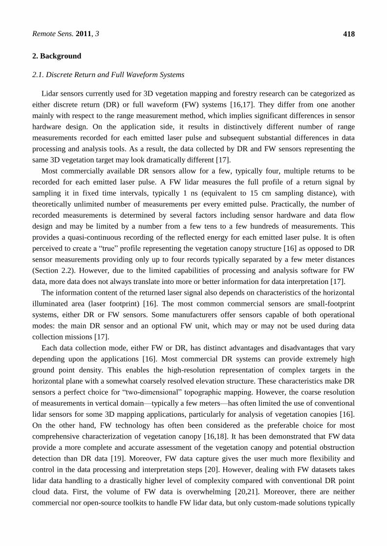
Figure 1(a,b) shows typical examples of multiple return vegetation data of two ALTM systems,
3100 and Gemini, which represent the most advanced models of the previous-generation ALTM series.
Although in both selected examples the minimal pulse return separation distances are relatively small,
1.5–2.2 m, it is apparent that only four discrete returns with a few-meter separation between them
cannot represent the vertical structure of vegetation properly. It was one of the reasons that until
recently FW sensors have often been the preferable choice for some vegetation mapping applications,
such as forestry research. However, the recent advances in DR lidar technology represented by a new
generation ALTM model, ALTM-Orion, may change some aspects of this situation.
Remote Sens. 2011, 3
421
Figure 1. Examples of four-return records from vegetation; (a) ALTM 3100; minimum
pulse return separation distance of 2.14 m; (b) ALTM Gemini: minimum pulse separation
distance of 1.54 m.
(a) (b)
The ALTM-Orion represents a radical departure from previous generations of airborne lidar sensors.
First, the physical form factor—size and weight—has been reduced by a whole order, making the
ALTM-Orion the first ultra-compact complete lidar solution with an optional UAV (unmanned aerial
vehicle) configuration [30]. Second, it has been shown [31] that the performance characteristics of the
ALTM-Orion include a few centimeter data elevation accuracy and precision for solid targets, as well
as for the data comprising small-size linear targets such as wires in power line corridors. In addition,
the new advanced design of the sensor transmitter and receiver hardware enabled to reduce the minimal
vertical target discrimination distance to sub-meter level, which has never been available before in any
commercial DR airborne lidar. In order to evaluate the performance and characterize the enhanced
capabilities of ALTM-Orion important for 3D vegetation mapping application, Optech Incorporated
has launched a series of studies presented below.
3.1. Objectives and Methodology
For the purpose of this study we selected several datasets collected by ALTM-Orion at 500 m flying
altitude over different types of vegetation targets. The ground point density was about 12 ppm2; the
laser pulse repetition frequency (equal to data collection rate) was kept at the maximum of 200 kHz for
all datasets. This study is based on the data collected over three areas of vegetation: a cornfield with an
average height 2.2–2.8 m and two nearby mixed forested areas with an average height of 6–7 m on one
side of the cornfield and 20–22 m on the other side. For the purpose of this study these datasets will be
referred in this paper as low-, medium- and high-canopy vegetation data. All datasets were collected by
the same ALTM-Orion system during the same data collection mission.
The objectives of this study include:
1. Empirical evaluation of the minimum vertical target discrimination distance for ALTM-Orion
data using statistical analysis of the field data collected over selected types of vegetation
targets.
Remote Sens. 2011, 3
422
2. Analysis of the capabilities of ALTM-Orion to represent the vertical structure of vegetation
targets: number and distribution of multiple returns, typical vertical target discrimination
values, correlation of number of multiple returns with vegetation height, signal penetration to
the ground.
3. Comparison of the results of 1–2 to a similar analysis based on ALTM-Gemini data.
4. Investigate the potential of return signal waveform modeling for DR data.
In order to achieve the aims of 1–3, several datasets of processed ALTM data were analyzed using
basic statistical tools, while lidar software visualization tools, such as Terrascan, were used for
verification and illustration of the results. The approach used for the return waveform modeling based
on analysis of DR data as well as some preliminary results and discussion, are presented in Section 4
describing the second part of this study.
3.2. Results and Discussion
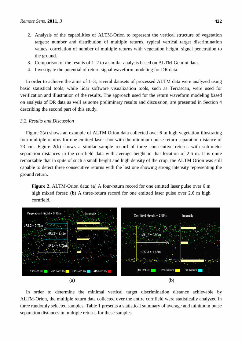
Figure 2(a) shows an example of ALTM Orion data collected over 6 m high vegetation illustrating
four multiple returns for one emitted laser shot with the minimum pulse return separation distance of
73 cm. Figure 2(b) shows a similar sample record of three consecutive returns with sub-meter
separation distances in the cornfield data with average height in that location of 2.6 m. It is quite
remarkable that in spite of such a small height and high density of the crop, the ALTM Orion was still
capable to detect three consecutive returns with the last one showing strong intensity representing the
ground return.
Figure 2. ALTM-Orion data: (a) A four-return record for one emitted laser pulse over 6 m
high mixed forest; (b) A three-return record for one emitted laser pulse over 2.6 m high
cornfield.
((a) (b)
In order to determine the minimal vertical target discrimination distance achievable by
ALTM-Orion, the multiple return data collected over the entire cornfield were statistically analyzed in
three randomly selected samples. Table 1 presents a statistical summary of average and minimum pulse
separation distances in multiple returns for these samples.
Remote Sens. 2011, 3
423
Table 1. ALTM-Orion: Average and minimal multiple return separation distances for the
cornfield data; the last column shows the average vegetation height in the selected samples.
Sample Avg ∆R1,2 (m) Avg ∆R2,3 (m) Avg ∆R3,4 (m) Avg height (m)
1 1.36 1.06 n/a 2.31
2 1.25 0.99 n/a 1.92
3 1.34 1.00 n/a 2.12
Sample Min ∆R1,2 (m) Min ∆R2,3 (m) Min ∆R3,4 (m) Avg height (m)
1 0.67 0.69 n/a 2.31
2 0.64 0.65 n/a 1.92
3 0.66 0.67 n/a 2.12
This summary clearly indicates that the minimal pulse return separation distances of ALTM-Orion
consistently fall within 0.64–0.67 m interval for all multiple returns. It also shows that there was no
single incidence of four-return record in all three samples of the cornfield data. This observation,
which may seem to be obvious, is in fact a clear indication that the number of multiple returns in
vegetation data is determined by the ratio between the vegetation height and minimum vertical target
discrimination capability of the lidar sensor.
Comparing the variations in average pulse return separation distances with changes in the total
cornfield height from sample to sample, one can also conclude that the second return R2 may be an
indicator of a change in the cornfield vertical structure while the last return R3 clearly indicates the
ground return. This is confirmed by the example of a three-return record presented in Figure 2(b),
which also shows that the second return, if detected from the middle if the cornfield mass, would have
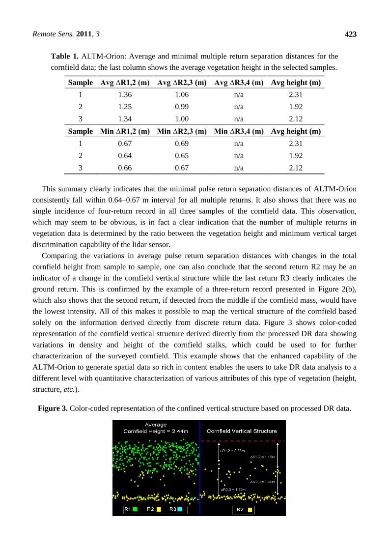
the lowest intensity. All of this makes it possible to map the vertical structure of the cornfield based
solely on the information derived directly from discrete return data. Figure 3 shows color-coded
representation of the cornfield vertical structure derived directly from the processed DR data showing
variations in density and height of the cornfield stalks, which could be used to for further
characterization of the surveyed cornfield. This example shows that the enhanced capability of the
ALTM-Orion to generate spatial data so rich in content enables the users to take DR data analysis to a
different level with quantitative characterization of various attributes of this type of vegetation (height,
structure, etc.).
Figure 3. Color-coded representation of the confined vertical structure based on processed DR data.
Remote Sens. 2011, 3
424
Table 2 shows a similar statistical summary for minimal and average pulse return separation
distances for the other datasets collected over mixed vegetation with average height of 6–7 m and
20–22 m. Comparing these results with those ones presented in Table 1, it is evident that the minimum
pulse return separation distances are not affected by the vegetation height and type and still fall mostly
within the same range 0.6–0.7 m. This indicates that this parameter does represent the system
capabilities rather than vegetation characteristics. On the other hand, average pulse separation
distances, and more significantly, number of multiple returns, are affected by the vegetation height and
type. This fact demonstrates that the resolution of the range measurements of a lidar system determines
the number of multiple returns over a vertical target, if a few discrete returns are covering the full
vertical extent of that target.
Table 2. ALTM-Orion: Average and minimum multiple return separation distances for the
forest data; the last column shows the average vegetation height in the selected samples.
Sample Avg ∆R1,2 (m) Avg ∆R2,3 (m) Avg ∆R3,4 (m) Avg height (m)
1 2.54 2.10 1.91 6.0
2 3.64 3.92 4.26 22.5
3 3.44 3.50 3.69 20.0
Sample Min ∆R1,2 (m) Min ∆R2,3 (m) Min ∆R3,4 (m) Avg height (m)
1 0.68 0.71 0.73 6.0
2 0.70 0.70 0.64 22.5
3 0.65 0.61 0.68 20.0
In order to correlate the vegetation height and the number of multiple returns, we ran another type of
statistical analysis for the mixed forest data. Table 3 presents the percentage of each multiple return in
the same randomly selected samples of the vegetation data.
Table 3. ALTM-Orion: Distribution of multiple returns for the mixed forest data.
Sample Pulse Return % of Total
Sample 1
Average height 6 m
1 55.88
2 33.03
3 9.38
4 1.71
Sample 2
Average height 22.5 m
1 43.22
2 31.6
3 17.71
4 7.47
Sample 3
Average height 20 m
1 44.8
2 31.91
3 16.79
4 6.51
Remote Sens. 2011, 3
425
First of all, this analysis confirms the correlation of the number of multiple returns with the
vegetation height, which was evident from the data presented in Tables 1 and 2: there are no fourth
returns in the cornfield data, while the system can consistently detect four returns from the vegetation
of 6 m height or more while operating at the same altitude with the same data collection parameters
during the same mission. Second, the numbers in Table 3 show that even small variations in the
vegetation height affect the number of the last returns and the distribution of multiple returns within
each data sample: the taller the vegetation canopy, the more third and fourth returns are detected.
Moreover, small variations the vegetation height (Samples 2 and 3, Table 3) are significant enough to
affect the distribution of the last returns.
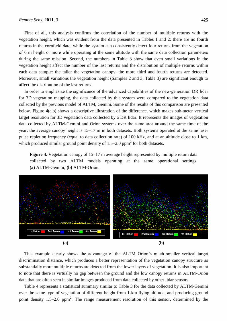
In order to emphasize the significance of the advanced capabilities of the new-generation DR lidar
for 3D vegetation mapping, the data collected by this system were compared to the vegetation data
collected by the previous model of ALTM, Gemini. Some of the results of this comparison are presented
below. Figure 4(a,b) shows a descriptive illustration of the difference, which makes sub-meter vertical
target resolution for 3D vegetation data collected by a DR lidar. It represents the images of vegetation
data collected by ALTM-Gemini and Orion systems over the same area around the same time of the
year; the average canopy height is 15–17 m in both datasets. Both systems operated at the same laser
pulse repletion frequency (equal to data collection rate) of 100 kHz, and at an altitude close to 1 km,
which produced similar ground point density of 1.5–2.0 ppm2 for both datasets.
Figure 4. Vegetation canopy of 15–17 m average height represented by multiple return data
collected by two ALTM models operating at the same operational settings.
(a) ALTM-Gemini; (b) ALTM-Orion.
(a) (b)
This example clearly shows the advantage of the ALTM Orion’s much smaller vertical target
discrimination distance, which produces a better representation of the vegetation canopy structure as
substantially more multiple returns are detected from the lower layers of vegetation. It is also important
to note that there is virtually no gap between the ground and the low canopy returns in ALTM-Orion
data that are often seen in similar images produced from data collected by other lidar sensors.
Table 4 represents a statistical summary similar to Table 3 for the data collected by ALTM-Gemini
over the same type of vegetation of different height from 1-km flying altitude, and producing ground
point density 1.5–2.0 ppm2. The range measurement resolution of this sensor, determined by the
Remote Sens. 2011, 3
426
system hardware design, depends on the sequential number of the multiple returns and varies within
1.5–2.5 m [32]. Based on the distribution of the multiple returns in this case, one can conclude that for
a tall vegetation canopy of 22–27 m, all four discrete returns are recorded, including the last one from
the ground beneath the vegetation canopy; the percentage of third and fourth returns is substantial.
However, for low-canopy vegetation of 6–7 m, the system cannot detect all four returns because of the
2.5 m minimal vertical target discrimination limit. The percentages of third and fourth returns for these
samples are negligible as the system cannot resolve any two targets in vertical domain within a distance
less than 2.5 m for the last two returns.
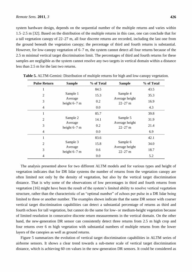
Table 5. ALTM-Gemini: Distribution of multiple returns for high and low-canopy vegetation.
Pulse Return Sample % of Total Sample % of Total
1
Sample 1
Average
height 6–7 m
84.5
Sample 4
Average height
22–27 m
43.5
2 15.3 35.3
3 0.2 16.9
4 0.0 4.3
1
Sample 2
Average
height 6–7 m
85.7
Sample 5
Average height
22–27 m
39.8
2 14.1 31.9
3 0.2 21.4
4 0.0 6.9
1
Sample 3
Average
height 6–7 m
83.6
Sample 6
Average height
22–27 m
42.1
2 15.8 34.0
3 0.6 18.7
4 0.0 5.2
The analysis presented above for two different ALTM models and for various types and height of
vegetation indicates that for DR lidar systems the number of returns from the vegetation canopy are
often limited not only by the density of vegetation, but also by the vertical target discrimination
distance. That is why some of the observations of low percentages in third and fourth returns from
vegetation [16] might have been the result of the system’s limited ability to resolve vertical vegetation
structure, rather than the characteristic of an ―optimal number‖ of echoes per pulse in a DR lidar being
limited to three or another number. The examples shown indicate that the same DR sensor with coarser
vertical target discrimination capabilities can detect a substantial percentage of returns as third and
fourth echoes for tall vegetation, but cannot do the same for low- or medium-height vegetation because
of limited resolution in consecutive discrete return measurements in the vertical domain. On the other
hand, the new-generation DR sensor can consistently detect three returns from 2.5 m high crop and
four returns over 6 m high vegetation with substantial numbers of multiple returns from the lower
layers of the canopies as well as ground returns.
Figure 5 summarizes the evolution of vertical target discrimination capabilities in ALTM series of
airborne sensors. It shows a clear trend towards a sub-meter scale of vertical target discrimination
distance, which is achieving 60 cm values in the new-generation DR sensors. It could be considered as
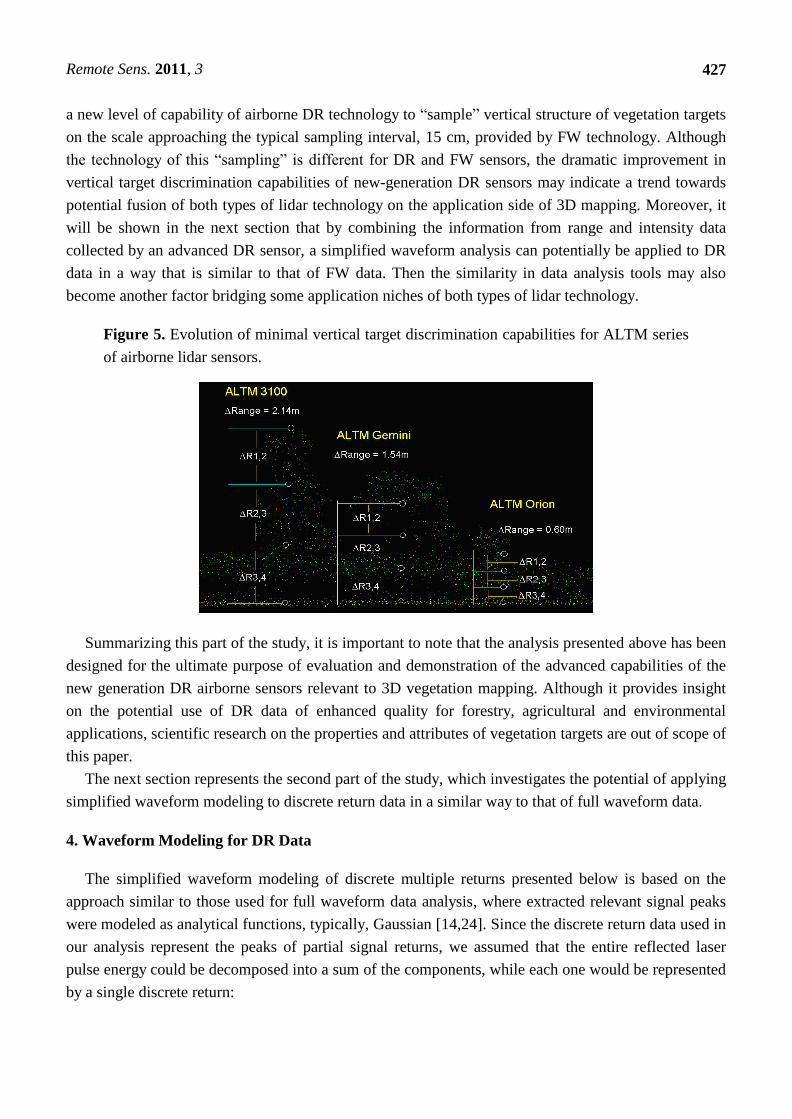
Remote Sens. 2011, 3
427
a new level of capability of airborne DR technology to ―sample‖ vertical structure of vegetation targets
on the scale approaching the typical sampling interval, 15 cm, provided by FW technology. Although
the technology of this ―sampling‖ is different for DR and FW sensors, the dramatic improvement in
vertical target discrimination capabilities of new-generation DR sensors may indicate a trend towards
potential fusion of both types of lidar technology on the application side of 3D mapping. Moreover, it
will be shown in the next section that by combining the information from range and intensity data
collected by an advanced DR sensor, a simplified waveform analysis can potentially be applied to DR
data in a way that is similar to that of FW data. Then the similarity in data analysis tools may also
become another factor bridging some application niches of both types of lidar technology.
Figure 5. Evolution of minimal vertical target discrimination capabilities for ALTM series
of airborne lidar sensors.
Summarizing this part of the study, it is important to note that the analysis presented above has been
designed for the ultimate purpose of evaluation and demonstration of the advanced capabilities of the
new generation DR airborne sensors relevant to 3D vegetation mapping. Although it provides insight
on the potential use of DR data of enhanced quality for forestry, agricultural and environmental
applications, scientific research on the properties and attributes of vegetation targets are out of scope of
this paper.
The next section represents the second part of the study, which investigates the potential of applying
simplified waveform modeling to discrete return data in a similar way to that of full waveform data.
4. Waveform Modeling for DR Data
The simplified waveform modeling of discrete multiple returns presented below is based on the
approach similar to those used for full waveform data analysis, where extracted relevant signal peaks
were modeled as analytical functions, typically, Gaussian [14,24]. Since the discrete return data used in
our analysis represent the peaks of partial signal returns, we assumed that the entire reflected laser
pulse energy could be decomposed into a sum of the components, while each one would be represented
by a single discrete return:
Remote Sens. 2011, 3
428
)()(1
xfxfn
i
i
(1)
Here n = 4 for four returns or 3 for three returns. For modeling of each function fi in our analysis we
used only a simple three-parametric Gaussian for all partial return for all vegetation types:
2
2
2
)(exp
i
iii
xaf
(2)
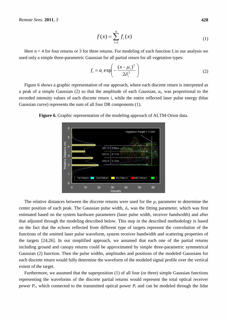
Figure 6 shows a graphic representation of our approach, where each discrete return is interpreted as
a peak of a simple Gaussian (2) so that the amplitude of each Gaussian, ai, was proportional to the
recorded intensity values of each discrete return i, while the entire reflected laser pulse energy (blue
Gaussian curve) represents the sum of all four DR components (1).
Figure 6. Graphic representation of the modeling approach of ALTM-Orion data.
The relative distances between the discrete returns were used for the µi parameter to determine the
center position of each peak. The Gaussian pulse width, δi, was the fitting parameter, which was first
estimated based on the system hardware parameters (laser pulse width, receiver bandwidth) and after
that adjusted through the modeling described below. This step in the described methodology is based
on the fact that the echoes reflected from different type of targets represent the convolution of the
functions of the emitted laser pulse waveform, system receiver bandwidth and scattering properties of
the targets [24,26]. In our simplified approach, we assumed that each one of the partial returns
including ground and canopy returns could be approximated by simple three-parametric symmetrical
Gaussian (2) function. Then the pulse widths, amplitudes and positions of the modeled Gaussians for
each discrete return would fully determine the waveform of the modeled signal profile over the vertical
extent of the target.
Furthermore, we assumed that the superposition (1) of all four (or three) simple Gaussian functions
representing the waveforms of the discrete partial returns would represent the total optical receiver
power Pr, which connected to the transmitted optical power Pt and can be modeled through the lidar
Remote Sens. 2011, 3
429
equation [33]. Considering partial signal returns Pi, the intensity (peak power) of each Gaussian pulse
was modeled using the lidar equation in the form derived by Jelalian [34]:
4
2
2
2
4 i
iatm
rti
RT
QDPP
(3)
Here:
Pi is the received signal power for i-return
Pt is the transmitted laser pulse power
Dr is the diameter of the lidar receiver aperture
Q is the optical efficiency of the lidar system
is the laser beam divergence
Tatm is the atmospheric transmittance factor
Ri is the range from the sensor to i-target
i is the effective backscattering cross-section of i-target
Here the reflective properties of each target for each partial return Pi are described by the
backscattering cross-section i, which is proportional to the i-target reflectance i and the i-fraction of
the total received power Pr in each return:
iiii Ak (4)
Here Ai is the area of the target illuminated by the i-fraction of the laser footprint, which created the
discrete return fi and ki is the fitting parameter, characterizing scattering properties of i-target, which
could be derived using redundant measurements. An approach similar in some aspects to this one was
applied to the analysis of full waveform data by Wagner and co-authors [24,35,36].
Based on the approach described by Equations (1–4), and using the known characteristics of the
ALTM-Orion hardware (emitted laser pulse characteristics, parameters of the receiver electronics and
optics), it was possible to model the total return optical power Pr through the lidar equation for a single
laser shot. Since Pr was assumed to be a superposition of all four (or three) partial returns Pi with a
simple Gaussian waveform, and knowing the intensities for each discrete return, it was possible to
model the amplitudes ai and pulse widths δi of each discrete return for the selected laser shots so that
the sum of the return pulse energies of all partial returns Pi would represent the pulse energy of the
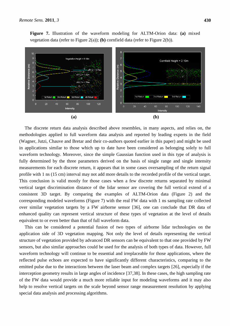
total return Pr. Figure 7 illustrates the results of the Gaussian waveform modeling for the samples of
multiple returns of the vegetation data presented earlier in Figure 2.
For such a consistent target as cornfield (Figure 7(b)) it also seemed to be possible to estimate the
effective reflectivity of the cornfield stalks through the Gaussian modeling of the corn and ground
returns. The blue dashed line in this figure represents the theoretical sum return that encompasses two
returns from vegetation, corn stalks, as opposed to the ground return with different reflective
properties. The histogram analysis of the intensity data consisting only of the same number of returns
(one, two or three returns) and reflected from the same type of target (corn as opposed to the ground)
showed consistent quasi-normal distribution of intensity values over sampled datasets. This work is
still in progress and requires more detailed analysis, but the preliminary results partly presented here
demonstrate a new potential of DR data analysis, which could potentially bridge the data analysis tools
used for both types of lidar technology.
Remote Sens. 2011, 3
430
Figure 7. Illustration of the waveform modeling for ALTM-Orion data: (a) mixed
vegetation data (refer to Figure 2(a)); (b) cornfield data (refer to Figure 2(b)).
(a) (b)
The discrete return data analysis described above resembles, in many aspects, and relies on, the
methodologies applied to full waveform data analysis and reported by leading experts in the field
(Wagner, Jutzi, Chauve and Bretar and their co-authors quoted earlier in this paper) and might be used
in applications similar to those which up to date have been considered as belonging solely to full
waveform technology. Moreover, since the simple Gaussian function used in this type of analysis is
fully determined by the three parameters derived on the basis of single range and single intensity
measurements for each discrete return, it appears that in some cases oversampling of the return signal
profile with 1 ns (15 cm) interval may not add more details to the recorded profile of the vertical target.
This conclusion is valid mostly for those cases when a few discrete returns separated by minimal
vertical target discrimination distance of the lidar sensor are covering the full vertical extend of a
consistent 3D target. By comparing the examples of ALTM-Orion data (Figure 2) and the
corresponding modeled waveforms (Figure 7) with the real FW data with 1 ns sampling rate collected
over similar vegetation targets by a FW airborne sensor [36], one can conclude that DR data of
enhanced quality can represent vertical structure of these types of vegetation at the level of details
equivalent to or even better than that of full waveform data.
This can be considered a potential fusion of two types of airborne lidar technologies on the
application side of 3D vegetation mapping. Not only the level of details representing the vertical
structure of vegetation provided by advanced DR sensors can be equivalent to that one provided by FW
sensors, but also similar approaches could be used for the analysis of both types of data. However, full
waveform technology will continue to be essential and irreplaceable for those applications, where the
reflected pulse echoes are expected to have significantly different characteristics, comparing to the
emitted pulse due to the interactions between the laser beam and complex targets [26], especially if the
interception geometry results in large angles of incidence [37,38]. In these cases, the high sampling rate
of the FW data would provide a much more reliable input for modeling waveforms and it may also
help to resolve vertical targets on the scale beyond sensor range measurement resolution by applying
special data analysis and processing algorithms.
Remote Sens. 2011, 3
431
Full waveform technology will also remain a preferable choice for 3D vegetation mapping that
requires the analysis of tall vegetation canopies (e.g., mature forest), as long as the number of multiple
discrete returns provided by advanced DR lidar systems is limited by four. In these cases only four
multiple discrete returns would leave wide gaps in the modeled vertical canopy profile. However, with
further development of DR and data handling technologies, when more than four discrete returns are
supported by both the lidar system hardware and the format of output data, it may become possible for
the DR and FW approach to give similar results in terms of representing 3D vegetation structure details
for some applications. Then it may become possible to develop new automated data analysis tools for
3D vegetation mapping bridging the academic research based on full waveform data analysis with the
workflow practices for discrete return data established in the commercial sector of lidar industry.
4. Conclusions
For the last two decades, the use of airborne lidar technology in certain 3D vegetation mapping
applications has often been based on analysis of the canopy profiles recorded by full waveform sensors.
The use of discrete return sensors for detailed representation on vertical vegetation structure has been
limited because of the coarse resolution of range measurements. The evolution of discrete return lidar
technology has achieved a new level of capabilities that approach those of full waveform technology in
representing 3D vegetation structure. The substantial reduction in vertical target discrimination
distance of new generation discrete return sensors may indicate a trend towards potential bridging of
both types of lidar technology on the application side of 3D vegetation mapping. The trade-off between
the high complexity and costs associated with full waveform data handling and analysis on the one
hand, and discrete return data of enhanced quality on the other hand, has the potential to create a new
application niche in the lidar industry with possible fusion of data analysis tools for both types of lidar
data. In this niche, high-quality dense discrete return point clouds, with fully recorded intensity
information for each of the multiple returns, may provide sufficient information for automated
modeling, analysis and quantitative characterization of 3D vegetation structure for a variety of
applications.
Acknowledgements
The authors are grateful to Brent Smith and Eric Yang for fruitful discussions.
References
1. Aldred, A.; Bonner, M. Application of Airborne Lasers to Forest Surveys; Information Report
PI-X-51; Petawawa National Forestry Centre, Canadian Forestry Service: Petawawa, ON, Canada,
1987; p. 62.
2. Nelson, R.; Krabill, W.; Maclean, G. Determining forest canopy characteristics using airborne
laser data. Remote Sens. Environ. 1984, 15, 201-212.
3. Dubayah, R.O.; Drake, J.B. Lidar remote sensing for forestry. J. Forestry 2000, 98, 44-46.
4. Nelson, R.; Parker, G.; Hom, M. A portable airborne laser system for forest inventory.
Photogramm. Eng. Remote Sensing 2003, 69, 267-273.
Remote Sens. 2011, 3
432
5. Roberts, S.D.; Dean, T.J.; Evans, D.L.; McCombs, J.W.; Harrington, R.L.; Glass, P.A. Estimating
individual tree leaf area in loblolly pine plantations using LiDAR-derived measurements of height
and crown dimensions. Forest Ecol. Manage. 2005, 213, 54-70.
6. Hudak, A.T.; Evans, J.S.; Smith, A.M.S. Review: LiDAR utility for natural resource managers.
Remote Sens. 2009, 1, 934-951.
7. Ussyshkin, V.; Theriault, L. Advances in Airborne Lidar Technology for Forestry and Other 3D
Mapping Applications. In Proceedings of the Regional ISPRS Conference: Latin American
Remote Sensing Week (LARS), Santiago, Chile, 4–7 October 2010.
8. Hopkinson, C.; Sitar, M.; Chasmer, L.; Treitz, P. Mapping snowpack depth beneath forest
canopies using airborne lidar. Photogramm. Eng. Remote Sensing 2004, 70, 323-330.
9. Alharthy, A.; Bethel, J. Heuristic Filtering and 3D Feature Extraction from Lidar Data. In
Proceedings of ISPRS Commission III, Symposium 2002 “Photogrammetric Computer Vision”,
Graz, Austria, 9–13 September 2002.
10. Bates, P.D.; Pappenberger, F.; Romanowicz, R. Uncertainty and risk in flood inundation
modeling. In Flood Forecasting; Beven, K., Hall, J., Eds.; Wiley & Co.: New York, NY, USA,
1999.
11. Raber, G.T.; Jensen, J.R.; Schill, S.R.; Schuckman, K. Creation of digital terrain models using an
adaptive Lidar vegetation point removal process. Photogramm. Eng. Remote Sensing 2002, 68,
1307-1316.
12. Renslow, M.; Greenfield, P.; Guay, T. Evaluation of Multi-Return LIDAR for Forestry
Applications; RSAC-2060/4810-LSP-0001-RPT1; US Department of Agriculture Forest
Service-Engineering: Salt Lake City, UT, USA, 2000; Available online: http://www.ndep.gov/
USDAFS_LIDAR.pdf (accessed on 19 November 2010).
13. Ussyshkin, V.; Sitar, M. Advantages of Airborne Lidar Technology for Power Line Asset
Management. In Proceedings of 5th Annual CIGRÉ Canada Conference: Innovation and
Renewal-Building the New Power System, Vancouver, BC, Canada, 17–19 October 2010;
[CDROM].
14. Chauve, A.; Mallet, C.; Bretar, F.; Durrieu, S.; Pierrot-Deseilligny, M.; Puech, W. Processing
Full-Waveform Lidar Data: Modelling Raw Signals. In Proceedings of ISPRS Workshop on Laser
Scanning 2007, Espoo, Finland, 12 September 2007; Volume 36, Part 3/W52, pp. 102-107.
15. Korpela, I.; Ørka, H.O.; Maltamo, M.; Tokola, T.; Hyyppä, J. Tree species classification using
airborne LiDAR—Effects of stand and tree parameters, downsizing of training set, intensity
normalization, and sensor type. Silva Fennica 2010, 44, 319-339.
16. Lim, K.; Treitz, P.; Wulder, M.; St-Onge, B.; Flood, M. LiDAR remote sensing of forest structure.
Progr. Phys. Geogr. 2003, 27, 88-106.
17. Parrish, C.E.; Scarpace, F.L. Investigation of Full Waveform Lidar Data for Detection and
Recognition of Vertical Objects. In Proceedings of ASPRS 2007 Annual Conference, Tampa, FL,
USA, 7–11 May 2007.
18. Chauve, A.; Vega, C.; Bretar, F.; Durrieu, S.; Allouis, T.; Pierrot-Deseilligny, M.; Puech, W.
Processing full-waveform lidar data in an alpine coniferous forest: assessing terrain and tree
height quality. Int. J. Remote Sens. 2009, 30, 5211-5228.
Remote Sens. 2011, 3
433
19. Magruder, L.A.; Neuenschwander, A.L.; Marmillion, S.P.; Tweddale, S.A. Obstruction detection
comparison of small-footprint full-waveform and discrete return lidar. Proc. SPIE 2010, 7684,
768410, doi:10.1117/12.850274.
20. Chauve, A.; Bretar, F.; Pierrot-Deseilligny, M.; Puech, W. Full Analyze: A Research Tool for
Handling, Processing and Analyzing Full-Waveform Lidar Data. In Proceedings of the 2009 IEEE
International Geoscience and Remote Sensing Symposium (IGARSS), Cape Town, South Africa,
12–17 July 2009.
21. Ussyshkin, V.; Theriault, L. ALTM-Orion: Bridging Conventional Lidar and Full Waveform
Digitizer Technology. In ISPRS TC VII Symposium “100 Years ISPRS”, Vienna, Austria, 5–7 July
2010; Volume 38, Part7B, pp. 606-611 [CDROM].
22. Bretar, F.; Chauve, A.; Mallet, C.; Jutzi, B. Managing Full Waveform Lidar Data: A Challenging
Task for the Forthcoming Years. In Proceeding sof XXIst ISPRS Congress, Beijing, China, 3–11
July 2008; Volume 37, Part B1, pp. 415-420.
23. Neuenschwander, A.L.; Magruder, L.A.; Tyler, M. Landcover classification of small-footprint,
full-waveform lidar data. J. Appl. Remote Sens. 2009, 3, 033544.
24. Wagner, W.; Hollaus, M.; Briese, C.; Ducic, V. 3D vegetation mapping using small-footprint
full-waveform airborne laser scanners. Int. J. Remote Sens. 2008, 29, 1433-1452.
25. Petrie, G. Current Developments in Airborne Laser Scanning Technologies. In Proceedings of IX
International Scientific & Technical Conference—From Imagery to Map: Digital
Photogrammetric Technologies, Attica, Greece, 5–8 October 2009.
26. Jutzi, B.; Stilla, U. Characteristics of the Measurement Unit of a Full-Waveform Laser System. In
Symposium of ISPRS Commission I: From Sensors to Imagery, Paris, France, May 2006;
Volume 36, Part 1/A, [CDROM].
27. Reitberger, J.; Krzystek, P.; Stilla, U. Analysis of Fullwaveform LiDAR Data for Tree Species
Classification. In Proceedings of ISPRS Symposium of Commission III “Photogrammetric
Computer Vision and Image Analysis”, Bonn, Germany, 20–22 September 2006; Volume 36,
pp. 228-233.
28. Jutzi, B.; Stilla, U. Range determination with waveform recording laser systems using a Wiener
Filter. ISPRS J. Photogramm. Remote Sens. 2006, 61, 95-107.
29. Hofton, M.A.; Blair, J.B. Laser altimeter return pulse correlation: A method for detecting surface
topographic change. J. Geodyn. 2002, 34, 477-489.
30. Hussein, M.; Tripp, J.; Hill, B. An ultra compact laser terrain mapper for deployment onboard
unmanned aerial vehicles. Proc. SPIE 2009, 7307, 73070B.
31. Ussyshkin, V.; Theriault, L. Precise Mapping: ALTM Orion Establishes a New Standard in
Airborne Lidar Performance. In Proceedings of ASPRS Annual Conference, San Diego, CA, USA,
26–30 April 2010.
32. Ussyshkin, V.; Theriault, L. Empirical Evaluation of the Resolution of Range Measurements in
ALTM-Gemini; Internal Optech Document; Optech: Vaughan, ON, Canada, 2010.
33. Measures, R.M. Laser Remote Sensing, Fundamentals and Applications; Wiley Interscience: New
York, NY, USA, 1984.
34. Jelalian, A.V. Laser Radar Systems; Artech House: Boston, MA, USA, 1992.
Remote Sens. 2011, 3
434
35. Wagner, W.; Ullrich, A.; Ducic, V.; Melzer, T.; Studnicka, N. Gaussian decomposition and
calibration of a novel small-footprint full-waveform digitising airborne laser scanner. ISPRS J.
Photogramm. Remote Sens. 2006, 60, 100-112.
36. Wagner, W.; Ullrich, A.; Melzer, T.; Briese, C.; Kraus, K. From Single-Pulse to Full-Waveform
Airborne Laser Scanners: Potential and Practical Challenges. In Proceedings of the International
Society for Photogrammetry and Remote Sensing 20th Congress Commission 3, Istanbul, Turkey,
12–23 July 2004; Volume 35, Part B/3, pp. 6-12.
37. Schaer, P.; Skaloud, J.; Landtwing, S.; Legat, K. Accuracy Estimation for Laser Point Cloud
Including Scanning Geometry. In Proceedings of The 5th International Symposium on Mobile
Mapping Technology, Padua, Italy, 29–31 May 2007.
38. Jutzi, B.; Gross, H. Normalization of Lidar Intensity Data Based on Range and Surface Incidence
Angle. In Proceedings of Laserscanning 09, Paris, France, 1–2 September 2009; Volume 38,
Part 3/W8, pp. 213-218.
© 2011 by the authors; licensee MDPI, Basel, Switzerland. This article is an open access article
distributed under the terms and conditions of the Creative Commons Attribution license
(http://creativecommons.org/licenses/by/3.0/).