Atmos. Chem. Phys., 13, 6023–6029, 2013www.atmos-chem-phys.net/13/6023/2013/doi:10.5194/acp-13-6023-2013© Author(s) 2013. CC Attribution 3.0 License.

EGU Journal Logos (RGB)

Advances in Geosciences

Open A

ccess

Natural Hazards and Earth System

Sciences

Open A

ccess

Annales Geophysicae

Open A

ccessNonlinear Processes

in Geophysics

Open A

ccess

Atmospheric Chemistry

and PhysicsO

pen Access

Atmospheric Chemistry

and Physics

Open A

ccess

Discussions

Atmospheric Measurement

Techniques

Open A

ccess

Atmospheric Measurement

Techniques

Open A

ccess

Discussions

Biogeosciences

Open A

ccess

Open A

ccess

BiogeosciencesDiscussions

Climate of the Past

Open A

ccess

Open A

ccess

Climate of the Past

Discussions

Earth System Dynamics

Open A

ccess

Open A

ccess

Earth System Dynamics

Discussions

GeoscientificInstrumentation

Methods andData Systems

Open A

ccess

GeoscientificInstrumentation

Methods andData Systems

Open A

ccess

Discussions

GeoscientificModel Development

Open A

ccess

Open A

ccess

GeoscientificModel Development

Discussions

Hydrology and Earth System

Sciences

Open A

ccess

Hydrology and Earth System

Sciences

Open A

ccess

Discussions

Ocean Science

Open A

ccess

Open A

ccess

Ocean ScienceDiscussions

Solid Earth

Open A

ccess

Open A

ccess

Solid EarthDiscussions

The Cryosphere

Open A

ccess

Open A

ccess

The CryosphereDiscussions

Natural Hazards and Earth System

Sciences

Open A

ccess

Discussions

Airborne lidar measurements of surface ozone depletion overArctic sea ice

J. A. Seabrook1, J. A. Whiteway1, L. H. Gray 1, R. Staebler2, and A. Herber3

1Centre for Research in Earth and Space Science (CRESS), York University, 4700 Keele Street, Toronto,Ontario, M3J 1P3, Canada2Environment Canada, 4905 Dufferin Street, Toronto, Ontario, M3H 5T4, Canada3Alfred Wegener Institute, Bussestrasse 24, 27570 Bremerhaven, Germany

Correspondence to:J. Whiteway (whiteway@yorku.ca)

Received: 31 October 2012 – Published in Atmos. Chem. Phys. Discuss.: 14 January 2013Revised: 16 May 2013 – Accepted: 18 May 2013 – Published: 22 June 2013

Abstract. A differential absorption lidar (DIAL) for mea-surement of atmospheric ozone concentration was operatedaboard the Polar 5 research aircraft in order to study the de-pletion of ozone over Arctic sea ice. The lidar measurementsduring a flight over the sea ice north of Barrow, Alaska, on3 April 2011 found a surface boundary layer depletion ofozone over a range of 300 km. The photochemical destruc-tion of surface level ozone was strongest at the most north-ern point of the flight, and steadily decreased towards land.All the observed ozone-depleted air throughout the flight oc-curred within 300 m of the sea ice surface. A back-trajectoryanalysis of the air measured throughout the flight indicatedthat the ozone-depleted air originated from over the ice. Airat the surface that was not depleted in ozone had originatedfrom over land. An investigation into the altitude history ofthe ozone-depleted air suggests a strong inverse correlationbetween measured ozone concentration and the amount oftime the air directly interacted with the sea ice.

1 Introduction

It has been observed that ozone becomes depleted in air nearthe sea ice surface during the polar sunrise period in the Arc-tic (e.g.,Oltmans, 1981; Oltmans and Komhyr, 1986; Botten-heim et al., 1986; Barrie et al., 1988, 1989; Seabrook et al.,2011) as well as the Antarctic (Jones et al., 2010). The obser-vations find episodes when the ozone mixing ratio at the sur-face decreases from the normal 30–40 ppbv to near zero forperiods ranging from hours to weeks at a time. The currently

accepted mechanism (Simpson et al., 2007) for the destruc-tion of tropospheric ozone involves bromine atoms originat-ing from activation of inert sea salt bromide ions in fresh seaice. Photochemical reactions convert the inert bromine intoreactive Br atoms that deplete ozone in the boundary layerin a catalytic reaction cycle known as a bromine explosion(Wennberg, 1999). This is consistent with the detection ofa strong inverse correlation between tropospheric ozone andfilterable Br (Barrie et al., 1989) and the coincident detec-tion of greater concentrations of BrO during ozone deple-tion events (Hausmann and Platt, 1994). The frequency andstrength of these ozone depletions has implications for theoverall mercury contamination of the snow/snowpack as theoxidation of gaseous elemental mercury (GEM) by Br and/orBrO, leading to the production of total particulate mercury(TPM) and reactive gaseous mercury (RGM), is strongly cor-related with ozone depletion events and the presence of reac-tive bromine (Lu et al., 2001; Steffen et al., 2008). McElroyet al.(1999) reported on measurements that indicated signif-icant amounts of BrO and thus depleted ozone in the Arcticfree troposphere. One of the aims of the study reported herewas to determine whether there was evidence for ozone de-pletion in air above the surface layer that is not directly incontact with the sea ice surface.

In order to investigate spatial structure of Arctic surfaceozone depletion events, a differential absorption, light de-tection and ranging instrument (differential absorption lidar,or DIAL) for the measurement of tropospheric ozone wasoperated from the Polar 5 research aircraft (Basler BT-67:rebuilt and modernized DC-3) as part of the PAMARCMIP

Published by Copernicus Publications on behalf of the European Geosciences Union.

6024 J. A. Seabrook et al.: Airborne lidar measurements of surface ozone depletion

2011 (Pan-Arctic Measurements and Arctic Regional climatemodel simulations) measurement campaign (Herber et al.,2012). Several flights out over the frozen Arctic Ocean werecarried out from Barrow, Alaska, during April 2011. The ob-served structure of the surface ozone depletion events alongthe flight track provided a unique view that has been appliedto assess the conditions in which the ozone depletion eventsoccur.

2 Measurement technique

The basic method was to emit pulses of light into the atmo-sphere and record the backscatter signal as a function of time,or equivalently range. For a UV wavelengthλ, absorbed sig-nificantly only by ozone, the backscatter signal is describedas

P (R,λ) =C

R2β (R,λ)exp

−2

R∫0

[σ (λ)n(R) + α (R,λ)]

dR, (1)

where P(R,λ) is the instantaneous received power fromrangeR. The backscatter coefficient,β(R,λ), represents thefraction of light scattered backward per unit length and perunit solid angle. The extinction coefficient,α (R,λ), is thefractional decrease in laser pulse intensity per unit length dueto scattering and absorption by molecules and aerosols. Theproduct of the ozone number density and absorption crosssection,σ (λ)n(R), is the fractional decrease in laser pulseenergy per unit length due to absorption by ozone molecules.C is a system constant that takes into account characteristicssuch as transmitted laser pulse energy, receiver aperture area,system optical throughput, and detector efficiency.

The lidar emitted multiple wavelengths in the UV thatlie on the broad Hartley ozone absorption band (266 nm,276 nm, 287 nm, 299 nm). The differential absorption be-tween wavelengths was employed to derive the ozone den-sity. Ozone retrieval from the recorded signal was performedby calculating the slope of the logarithmic ratio of any pairof these signals as

n(R) =−1

2(σ (λon) − σ (λoff))(2){

d

dR

[ln

(Pon(R)

Poff (R)

)]+ 2(αm (R,λon) − αm (R,λoff))

},

where “on” denotes the wavelength with the largerozone absorption cross section, and the term2(αm (R,λon) − αm (R,λoff)) is a correction factor toaccount for differential extinction due to molecular scatter-ing. Ozone was derived using the temperature-dependentozone absorption cross sections from the HITRAN 2008database (Rothman et al., 2009).

For the measurements in this study, there was not a sig-nificant contribution to the signal by aerosol and cloud par-ticles, and the differential absorption and scattering due to

PMTs

transientrecorder

PC

interferencefilters15 cm

telescope opticalfiber

mirrors

Nd:YAGlaser

266 nm

CO

2 R

aman

cel

l

beamexpander

Output266 nm276 nm287 nm299 nm

lens 1

lens 2

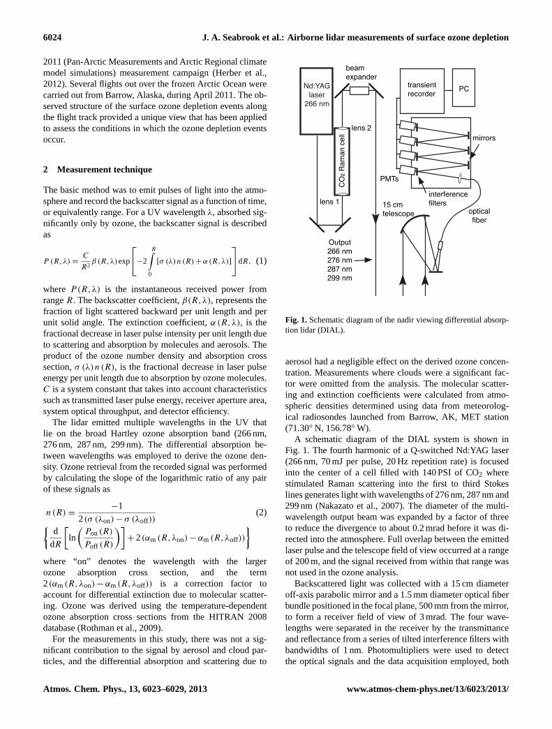
Fig. 1. Schematic diagram of the nadir viewing differential absorp-tion lidar (DIAL).

aerosol had a negligible effect on the derived ozone concen-tration. Measurements where clouds were a significant fac-tor were omitted from the analysis. The molecular scatter-ing and extinction coefficients were calculated from atmo-spheric densities determined using data from meteorolog-ical radiosondes launched from Barrow, AK, MET station(71.30◦ N, 156.78◦ W).

A schematic diagram of the DIAL system is shown inFig. 1. The fourth harmonic of a Q-switched Nd:YAG laser(266 nm, 70 mJ per pulse, 20 Hz repetition rate) is focusedinto the center of a cell filled with 140 PSI of CO2 wherestimulated Raman scattering into the first to third Stokeslines generates light with wavelengths of 276 nm, 287 nm and299 nm (Nakazato et al., 2007). The diameter of the multi-wavelength output beam was expanded by a factor of threeto reduce the divergence to about 0.2 mrad before it was di-rected into the atmosphere. Full overlap between the emittedlaser pulse and the telescope field of view occurred at a rangeof 200 m, and the signal received from within that range wasnot used in the ozone analysis.

Backscattered light was collected with a 15 cm diameteroff-axis parabolic mirror and a 1.5 mm diameter optical fiberbundle positioned in the focal plane, 500 mm from the mirror,to form a receiver field of view of 3 mrad. The four wave-lengths were separated in the receiver by the transmittanceand reflectance from a series of tilted interference filters withbandwidths of 1 nm. Photomultipliers were used to detectthe optical signals and the data acquisition employed, both

Atmos. Chem. Phys., 13, 6023–6029, 2013 www.atmos-chem-phys.net/13/6023/2013/

J. A. Seabrook et al.: Airborne lidar measurements of surface ozone depletion 6025

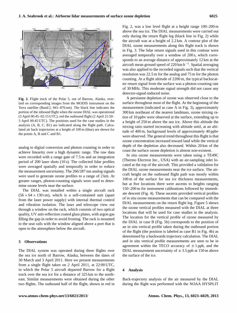
Fig. 2. Flight track of the Polar 5, out of Barrow, Alaska, over-laid on corresponding images from the MODIS instrument on theTerra satellite (Band 2, 841–876 nm). The black line indicates theportion of the inbound flight when the ozone DIAL was operational(3 April 00:45–02:15 UTC), red the outbound flight (2 April 21:50–3 April 00:45 UTC). The positions used for the case studies in theanalysis (A, B, C, B1) are indicated along the flight path. Calcu-lated air back trajectories at a height of 100 m (blue) are shown forthe points A, B and C and B1.

analog to digital conversion and photon counting in order toachieve linearity over a high dynamic range. The raw datawere recorded with a range gate of 7.5 m and an integrationperiod of 200 laser shots (10 s). The collected lidar profileswere averaged spatially and temporally in order to reducethe measurement uncertainty. The 266/287 nm analog signalswere used to generate ozone profiles to a range of 2 km. Atgreater ranges, photon-counting signals were used to deter-mine ozone levels near the surface.

The DIAL was installed within a single aircraft rack(56× 64× 130 cm), which is a self-contained unit (apartfrom the laser power supply) with internal thermal controland vibration isolation. The laser and telescope view outthrough a window on the rack, which consists of two opticalquality, UV anti-reflection coated glass plates, with argon gasfilling the gap in order to avoid frosting. The rack is mountedto the seat rails with the window aligned above a port that isopen to the atmosphere below the aircraft.

3 Observations

The DIAL system was operated during three flights overthe sea ice north of Barrow, Alaska, between the dates of30 March and 3 April 2011. Here we present measurementsfrom a single flight taken on 2 April 2011, at 22:00 UTC,in which the Polar 5 aircraft departed Barrow for a flighttrack over the sea ice for a distance of 325 km to the north-east. Similar measurements were obtained during the othertwo flights. The outbound half of the flight, shown in red in

Fig. 2, was a low level flight at a height range 100–200 mabove the sea ice. The DIAL measurements were carried outonly during the return flight leg (black line in Fig.2) whilethe aircraft was at a height of 2.2 km. A contour plot of theDIAL ozone measurements along this flight track is shownin Fig. 3. The lidar return signals used in this contour wereaveraged temporally over a window of 200 s, which corre-sponds to an average distance of approximately 12 km at theaircraft mean ground speed of 220 km h−1. Spatial averagingwas also applied to the recorded signals such that the verticalresolution was 22.5 m for the analog and 75 m for the photoncounting. At a flight altitude of 2200 m, the typical backscat-ter return signal from the surface was a photon-counting rateof 30 MHz. This moderate signal strength did not cause anydetector-signal-induced noise.

A persistent depletion of ozone was observed close to thesurface throughout most of the flight. At the beginning of themeasurement (indicated as case A in Fig.3), approximately300 km northeast of the nearest landmass, ozone mixing ra-tios of 10 ppbv were observed at the surface, extending up toa height of 250 m above the sea ice. Above this altitude themixing ratio started increasing with altitude until, at an alti-tude of 400 m, background levels of approximately 40 ppbvwere observed. The general trend throughout this flight is thatozone concentration increased toward land while the verticaldepth of the depletion also decreased. Within 20 km of thecoast the surface ozone depletion is almost non-existent.

In situ ozone measurements were taken using a TE49C(Thermo Electron Inc., USA) with an air-sampling inlet lo-cated at the top of the aircraft. This provided a validation forthe DIAL ozone measurements near the ice surface. The air-craft height on the outbound flight path was mostly within100 m of the surface for sea ice thickness measurements,but at five locations there were ascents to heights ranging150–200 m for instrument calibrations followed by immedi-ate descent (Fig.4). These ascents provided vertical profilesof in situ ozone measurements that can be compared with theDIAL measurements on the return flight leg. Figure5 showsthe ozone vertical profiles measured with the DIAL at threelocations that will be used for case studies in the analysis.The location for the vertical profile of ozone measured bythe DIAL in case B (Fig.5b) corresponds to the position ofan in situ vertical profile taken during the outbound portionof the flight (the position is labeled as case B1 in Fig.4b) asdetermined by a backwards trajectory calculation. The DIALand in situ vertical profile measurements are seen to be inagreement within the TECO accuracy of± 1 ppb, and theDIAL measurement uncertainty of± 3.5 ppb at 150 m abovethe surface of the ice.

4 Analysis

Back-trajectory analysis of the air measured by the DIALduring the flight was performed with the NOAA HYSPLIT

www.atmos-chem-phys.net/13/6023/2013/ Atmos. Chem. Phys., 13, 6023–6029, 2013

6026 J. A. Seabrook et al.: Airborne lidar measurements of surface ozone depletion

Fig. 3. DIAL measurements of ozone mixing ratio along the track of the aircraft shown in Fig. reffigure2. Lines labeled(A), (B) and(C)correspond to the positions of the aircraft labeled in Fig.2, where the corresponding air back trajectories have been calculated.

01020304050

In-s

ituoz

one

(ppb

v )

0.0

0.2

0.4

0.6

Airc

raft

altit

ude

(km

)

300 250 200 150 100 50 0Distance from the coast (km)

a

bB1

Fig. 4. (a) In situ ozone measurements along the outbound flighttrack (black trace in Fig.2) with the distance from the coast ofAlaska. (b) Aircraft altitude along the outbound flight track. B1indicates the position of the aircraft during the outbound flight aslabeled in Fig.2.

model (Draxler and Hess., 1998), using GDAS (Global DataAssimilation System) meteorological data. The historicalback trajectories were calculated every two minutes for theperiod of time in which the DIAL was active for heightsranging from 100 m to 2000 m a.s.l. and were calculated fora 6-day period backward starting from the GPS location ofthe aircraft at each time interval.

The period of time in which the strongest depletion wasobserved (case A) occurred at the northernmost extent of theflight track, approximately 300 km from the northern tip ofAlaska (indicated as case A in Fig.3). The ozone-mixingratio was less than 10 ppbv up to a height of 250 m and thenincreased to the background level of 30–40 ppbv at a heightof 400 m. In this case the back trajectories shown in Fig.6a

0 10 20 30 40 50

0.0

0.4

0.8

1.2

1.6

Hei

ght a

.s.l.

(km

)

A

0 10 20 30 40 50

BDIAL

In situ

0 10 20 30 40 50

Ozone (ppbv)

C

Fig. 5. Measured vertical profiles of ozone mixing ratio with theDIAL along the inbound flight track, and in situ measurements (grayline) along the outbound flight track (position B1 in Figs.2 and4b.). Cases (A), (B), and (C) correspond to the positions indicated inFigs.2 and3. The indicated uncertainty in the DIAL measurementis one standard deviation in the photon counts, propagated throughthe ozone derivation.

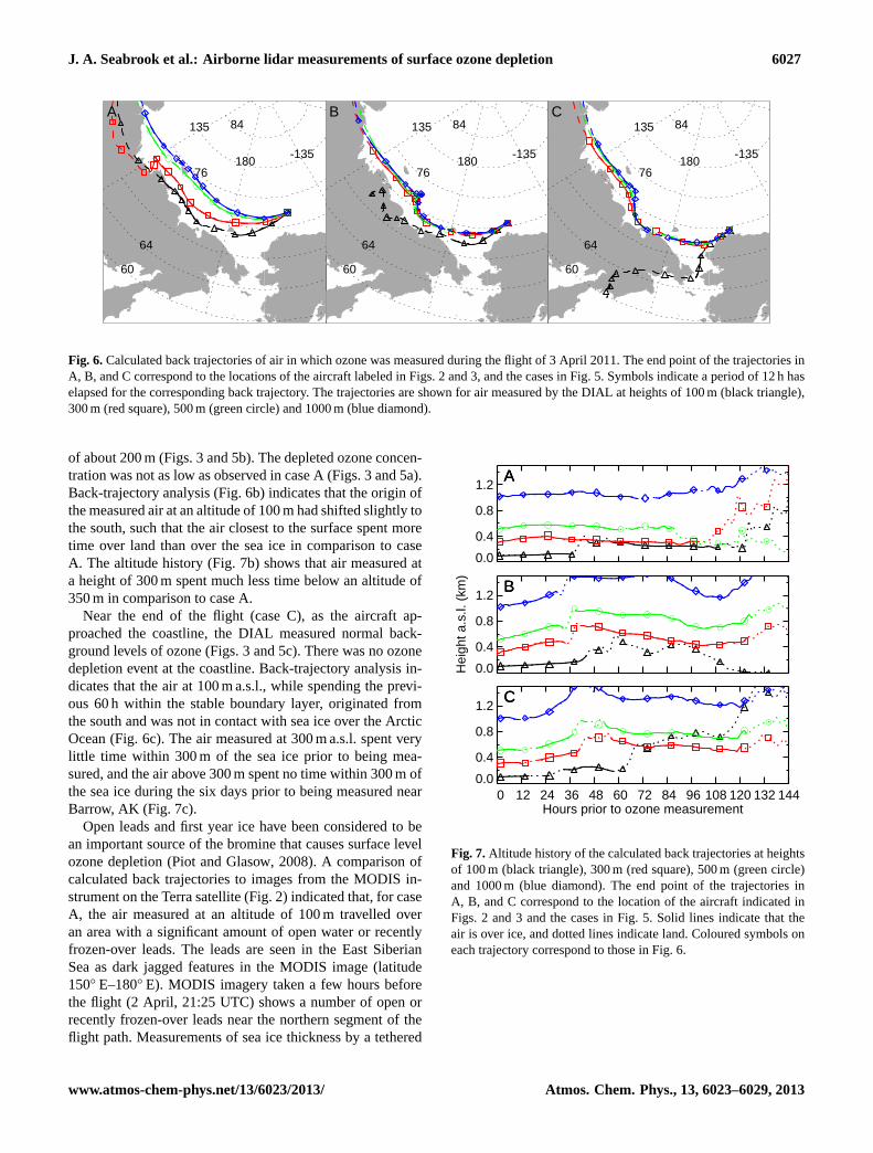
indicate that the air up to a height of 1000 m originated fromthe west over the Arctic sea ice. An analysis of the altitudehistory for case A (Fig.7a) indicates that the air at 100 mand 300 m above the ice surface had spent significant timebelow 350 m in the previous days, while the back trajectoriesstarting at heights of 500 m and 1000 m did not spend anytime below 350 m in the previous six days.

In case B, approximately 140 km from land, the ozone de-pletion was observed to extend from the surface to a height

Atmos. Chem. Phys., 13, 6023–6029, 2013 www.atmos-chem-phys.net/13/6023/2013/

J. A. Seabrook et al.: Airborne lidar measurements of surface ozone depletion 6027

135

180-135

84

76

64

60

A135

180-135

84

76

64

60

B135

180-135

84

76

64

60

C

Fig. 6.Calculated back trajectories of air in which ozone was measured during the flight of 3 April 2011. The end point of the trajectories inA, B, and C correspond to the locations of the aircraft labeled in Figs. 2 and 3, and the cases in Fig. 5. Symbols indicate a period of 12 h haselapsed for the corresponding back trajectory. The trajectories are shown for air measured by the DIAL at heights of 100 m (black triangle),300 m (red square), 500 m (green circle) and 1000 m (blue diamond).

of about 200 m (Figs.3 and5b). The depleted ozone concen-tration was not as low as observed in case A (Figs.3 and5a).Back-trajectory analysis (Fig.6b) indicates that the origin ofthe measured air at an altitude of 100 m had shifted slightly tothe south, such that the air closest to the surface spent moretime over land than over the sea ice in comparison to caseA. The altitude history (Fig.7b) shows that air measured ata height of 300 m spent much less time below an altitude of350 m in comparison to case A.

Near the end of the flight (case C), as the aircraft ap-proached the coastline, the DIAL measured normal back-ground levels of ozone (Figs.3 and5c). There was no ozonedepletion event at the coastline. Back-trajectory analysis in-dicates that the air at 100 m a.s.l., while spending the previ-ous 60 h within the stable boundary layer, originated fromthe south and was not in contact with sea ice over the ArcticOcean (Fig.6c). The air measured at 300 m a.s.l. spent verylittle time within 300 m of the sea ice prior to being mea-sured, and the air above 300 m spent no time within 300 m ofthe sea ice during the six days prior to being measured nearBarrow, AK (Fig.7c).

Open leads and first year ice have been considered to bean important source of the bromine that causes surface levelozone depletion (Piot and Glasow, 2008). A comparison ofcalculated back trajectories to images from the MODIS in-strument on the Terra satellite (Fig.2) indicated that, for caseA, the air measured at an altitude of 100 m travelled overan area with a significant amount of open water or recentlyfrozen-over leads. The leads are seen in the East SiberianSea as dark jagged features in the MODIS image (latitude150◦ E–180◦ E). MODIS imagery taken a few hours beforethe flight (2 April, 21:25 UTC) shows a number of open orrecently frozen-over leads near the northern segment of theflight path. Measurements of sea ice thickness by a tethered

0.0

0.4

0.8

1.2

AAA

0.0

0.4

0.8

1.2

Hei

ght a

.s.l.

(km

)

BBB

0 12 24 36 48 60 72 84 96 108 120 132 144Hours prior to ozone measurement

0.0

0.4

0.8

1.2

CCC

Fig. 7.Altitude history of the calculated back trajectories at heightsof 100 m (black triangle), 300 m (red square), 500 m (green circle)and 1000 m (blue diamond). The end point of the trajectories inA, B, and C correspond to the location of the aircraft indicated inFigs. 2 and3 and the cases in Fig.5. Solid lines indicate that theair is over ice, and dotted lines indicate land. Coloured symbols oneach trajectory correspond to those in Fig.6.

www.atmos-chem-phys.net/13/6023/2013/ Atmos. Chem. Phys., 13, 6023–6029, 2013

6028 J. A. Seabrook et al.: Airborne lidar measurements of surface ozone depletion

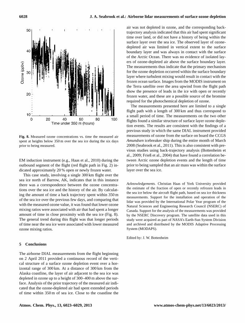
Fig. 8. Measured ozone concentrations vs. time the measured airspent at heights below 350 m over the sea ice during the six daysprior to being measured.

EM induction instrument (e.g.,Haas et al., 2010) during theoutbound segment of the flight (red flight path in Fig.2) in-dicated approximately 20 % open or newly frozen water.

This case study, involving a single 300 km flight over thesea ice north of Barrow, AK, indicates that in this instancethere was a correspondence between the ozone concentra-tions over the sea ice and the history of the air. By calculat-ing the amount of time a back trajectory spent within 350 mof the sea ice over the previous few days, and comparing thatwith the measured ozone value, it was found that lower ozonemixing ratios were associated with air that had spent a longeramount of time in close proximity with the sea ice (Fig.8).The general trend during this flight was that longer periodsof time near the sea ice were associated with lower measuredozone mixing ratios.

5 Conclusions

The airborne DIAL measurements from the flight beginningon 2 April 2011 provided a continuous record of the verti-cal structure of a surface ozone depletion event over a hor-izontal range of 300 km. At a distance of 300 km from theAlaska coastline, the layer of air adjacent to the sea ice wasdepleted in ozone up to a height of 300–400 m above the sur-face. Analysis of the prior trajectory of the measured air indi-cated that the ozone-depleted air had spent extended periodsof time within 350 m of sea ice. Close to the coastline the

air was not depleted in ozone, and the corresponding back-trajectory analysis indicated that this air had spent significanttime over land, or did not have a history of being within thesurface layer over the sea ice. The observed layer of ozone-depleted air was limited in vertical extent to the surfaceboundary layer and was always in contact with the surfaceof the Arctic Ocean. There was no evidence of isolated lay-ers of ozone-depleted air above the surface boundary layer.The measurements thus indicate that the primary mechanismfor the ozone depletion occurred within the surface boundarylayer where turbulent mixing would result in contact with thefrozen ocean surface. Images from the MODIS instrument onthe Terra satellite over the area upwind from the flight pathshow the presence of leads in the ice with open or recentlyfrozen water, and these are a possible source of the brominerequired for the photochemical depletion of ozone.

The measurements presented here are limited to a singleflight path with a length of 300 km and thus correspond toa small period of time. The measurements on the two otherflights found a similar structure of surface layer ozone deple-tion events. The results are consistent with the findings of aprevious study in which the same DIAL instrument providedmeasurements of ozone from the surface on board the CCGSAmundsenicebreaker ship during the entire month of March2008 (Seabrook et al., 2011). This is also consistent with pre-vious studies using back-trajectory analysis (Bottenheim etal., 2009; Frieß et al., 2004) that have found a correlation be-tween Arctic ozone depletion events and the length of timeprior to being sampled that an air mass was within the surfacelayer over the sea ice.

Acknowledgements.Christian Haas of York University providedthe estimate of the fraction of open or recently refrozen leads inthe sea ice below the aircraft flight path, based on sea ice thicknessmeasurements. Support for the installation and operation of thelidar was provided by the International Polar Year program of theNatural Sciences and Engineering Research Council (NSERC) ofCanada. Support for the analysis of the measurements was providedby the NSERC Discovery program. The satellite data used in thisstudy were acquired as part of NASA’s Earth-Sun System Divisionand archived and distributed by the MODIS Adaptive ProcessingSystem (MODAPS).

Edited by: J. W. Bottenheim

Atmos. Chem. Phys., 13, 6023–6029, 2013 www.atmos-chem-phys.net/13/6023/2013/

J. A. Seabrook et al.: Airborne lidar measurements of surface ozone depletion 6029

References

Barrie, L., Bottenheim, J., Schnell, R., Crutzen, P., and Rasmussen,R.: Ozone destruction and photochemical reactions at polar sun-rise in the lower Arctic atmosphere, Nature, 334, 138–141,doi:10.1038/334138a0, 1988.

Barrie, L., Hartog, G., Bottenheim, J., and Landsberger, S.: An-thropogenic aerosols and gases in the lower troposphere atAlert Canada in April 1986, J. Atmos. Chem., 9, 101–127,doi:10.1007/BF00052827, 1989.

Bottenheim, J., Gallant, A., and Brice, K.: Measurements of NOY

species and O3 at 82◦ N latitude, Geophys. Res. Lett., 13, 113–116, doi:10.1029/GL013i002p00113, 1986.

Bottenheim, J., Netcheva, S., Morin, S., and Nghiem, S.: Ozone inthe boundary layer air over the Arctic Ocean: measurements dur-ing the TARA transpolar drift 2006–2008, Atmos. Chem. Phys.,9, 4545–4557, doi:10.5194/acp-9-4545-2009, 2009.

Draxler, R., and Hess, G.: An overview of the HYSPLIT 4 mod-elling system for trajectories, dispersion, and deposition, Aust.Meteorol. Mag., 47, 295–308, 1998.

Frieß, U., Hollwedel, J., Konig-Langlo, G., Wagner, T., and Platt,U.: Dynamics and chemistry of tropospheric bromine explosionevents in the Antarctic coastal region, J. Geophys. Res., 109,D06305, doi:10.1029/2003JD004133, 2004.

Haas, C., Hendricks, S., Eicken, H., and Herber, A.: Synoptic air-borne thickness surveys reveal state of Arctic sea ice cover, Geo-phys. Res. Lett., 37, doi:10.1029/2010GL042652, 2010.

Hausmann, M., and Platt, U.: Spectroscopic measurement ofbromine oxide and ozone in the high Arctic during Polar Sun-rise Experiment 1992, J. Geophys. Res., 99, 25399–25413,doi:10.1029/94JD01314, 1994.

Herber, A. B., Hass, C., Stone, R. S., Bottenheim, J. W., Liu, P., Li,S.-M., Staebler, R. M., Strapp, J. W., and Dethloff, K.: Regularairborne surveys of Arctic sea ice and atmosphere, Eos Trans.AGU, 93, 41, doi:10.1029/2012EO040001, 2012.

Jones, A., Anderson, P., Wolff, E., Roscoe, H., Marshall, G.,Richter, A., Brough, N., and Colwell, S.: Vertical structure ofAntarctic tropospheric ozone depletion events: characteristicsand broader implications, Atmos. Chem. Phys., 10, 7775–7794,doi:10.5194/acp-10-7775-2010, 2010.

Lu, J. Y., Schroeder, W. H., Barrie, L. A., Steffen, A., Welch,H. E., Martin, K., Lockhart, L., Hunt, R. V., Boila, G., andRichter, A.: Magnification of atmospheric mercury deposi-tion to polar regions in springtime: The link to troposphericozone depletion chemistry, Geophys. Res. Lett., 28, 3219–3222,doi:10.1029/2000GL012603, 2001.

McElroy, C. T., McLinden, C. A., and McConnell, J. C.: Evidencefor bromine monoxide in the free troposphere during the Arcticpolar sunrise, Nature, 397, 338–341, doi:10.1038/16904, 1999.

Nakazato, M., Nagai, T., Sakai, T., and Hirose, Y.: Tropo-spheric ozone differential-absorption lidar using stimulated Ra-man scattering in carbon dioxide, Appl. Optics, 46, 2269–2279,doi:10.1364/AO.46.002269, 2007.

Oltmans, S.: Surface ozone measurements in clean air, J. Geophys.Res., 86, 1174–1180, doi:10.1029/JC086iC02p01174, 1981.

Oltmans, S., and Komhyr, W.: Surface ozone distributions and vari-ations from 1973–1984 measurements at the NOAA geophys-ical monitoring for climatic change baseline observatories, J.Geophys. Res., 91, 5229–5236, doi:10.1029/JD091iD04p05229,1986.

Piot, M., and von Glasow, R.: The potential importance of frostflowers, recycling on snow, and open leads for ozone depletionevents, Atmos. Chem. Phys., 8, 2437–2467, doi:10.5194/acp-8-2437-2008, 2008.

Rothman, L., Gordon, I., and Barbe, A.: The HITRAN 2008 molec-ular spectroscopic database, J. Quant. Spectrosc. Ra., 110, 533–572, doi:10.1016/j. jqsrt.2009.02.013, 2009.

Seabrook, J. A., Whiteway, J., Staebler, R. M., Bottenheim, J. W.,Komguem, L., Gray, L. H., Barber, D., and Asplin, M.: LI-DAR measurements of Arctic boundary layer ozone depletionevents over the frozen Arctic Ocean, J. Geophys. Res., 116,doi:10.1029/2011JD016335, 2011.

Simpson, W. R., et al.: Halogens and their role in polar bound-ary layer ozone depletion, Atmos. Chem. Phys., 7, 4375–4418,doi:10.5194/acp-7-4375-2007, 2007.

Steffen, A., Douglas, T., Amyot, M., Ariya, P., Aspmo, K., Berg, T.,Bottenheim, J., Brooks, S., Cobbett, F., Dastoor, A., Dommergue,A., Ebinghaus, R., Ferrari, C., Gardfeldt, K., Goodsite, M. E.,Lean, D., Poulain, A. J., Scherz, C., Skov, H., Sommar, J., andTemme, C.: A synthesis of atmospheric mercury depletion eventchemistry in the atmosphere and snow, Atmos. Chem. Phys., 8,1445–1482, doi:10.5194/acp-8-1445-2008, 2008.

Wennberg, P.: Atmospheric chemistry: Bromine explosion, Nature,397, 299–301, doi:10.1038/16805, 1999.

www.atmos-chem-phys.net/13/6023/2013/ Atmos. Chem. Phys., 13, 6023–6029, 2013