Aircraft Fuel Consumption – Estimation and …...DEPARTMENT OF AUTOMOTIVE AND AERONAUTICAL ENGINEERING Aircraft Fuel Consumption – Estimation and Visualization Task for a Project

1

Project

Aircraft Fuel Consumption – Estimation and Visualization

Author: Marcus Burzlaff

Supervisor: Prof. Dr.-Ing. Dieter Scholz, MSME Delivery Date: 13.12.2017

Faculty of Engineering and Computer Science

Department of Automotive and Aeronautical Engineering

URN: http://nbn-resolving.org/urn:nbn:de:gbv:18302-aero2017-12-13.019 Associated URLs: http://nbn-resolving.org/html/urn:nbn:de:gbv:18302-aero2017-12-13.019

© This work is protected by copyright

The work is licensed under a Creative Commons Attribution-NonCommercial-ShareAlike 4.0

International License: CC BY-NC-SA

http://creativecommons.org/licenses/by-nc-sa/4.0

Any further request may be directed to:

Prof. Dr.-Ing. Dieter Scholz, MSME

E-Mail see: http://www.ProfScholz.de

This work is part of:

Digital Library - Projects & Theses - Prof. Dr. Scholz

http://library.ProfScholz.de

Published by

Aircraft Design and Systems Group (AERO)

Department of Automotive and Aeronautical Engineering

Hamburg University of Applied Science

This report is deposited and archived:

Deutsche Nationalbiliothek (http://www.dnb.de)

Repositorium der Leibniz Universität Hannover (http://www.repo.uni-hannover.de)

This report has associated published data in Harvard Dataverse:

http://doi.org/10.7910/DVN/2HMEHB

Abstract

In order to uncover the best kept secret in today’s commercial aviation, this project deals with

the calculation of fuel consumption of aircraft. With only the reference of the aircraft manu-

facturer’s information, given within the airport planning documents, a method is established

that allows computing values for the fuel consumption of every aircraft in question. The air-

craft's fuel consumption per passenger and 100 flown kilometers decreases rapidly with range,

until a near constant level is reached around the aircraft’s average range. At longer range,

where payload reduction becomes necessary, fuel consumption increases significantly. Nu-

merical results are visualized, explained, and discussed. With regard to today’s increasing

number of long-haul flights, the results are investigated in terms of efficiency and viability.

The environmental impact of burning fuel is not considered in this report. The presented

method allows calculating aircraft type specific fuel consumption based on publicly available

information. In this way, the fuel consumption of every aircraft can be investigated and can be

discussed openly.

DEPARTMENT OF AUTOMOTIVE AND AERONAUTICAL ENGINEERING

Aircraft Fuel Consumption –

Estimation and Visualization

Task for a Project according to university regulations.

Background

"3.85 liters per 100 passenger kilometers” – this was Lufthansa Group's specific fuel

consumption in 2016, averaged over short-haul and long-haul flights. The statement was

taken from Lufthansa Group's Sustainability Report 2017. The amount of consumed fuel

depends on different factors: aircraft type, distance, payload, cruise Mach number, and more.

It is evident: a) The longer the distance flown, the more fuel will be consumed. b) Is fuel

consumption sufficiently constant versus range, if the fuel consumption is calculated per

range? c) How does the picture change if we consider fuel consumption per range and per

number of seats? Consider: Payload (and hence number of passengers) has to be reduced for

flights at very long range. A nonlinear behavior is found for specific fuel consumption plotted

versus range in all the cases mentioned. The problem: Publicly available aircraft data is

always limited.

Task

Task of this project is to extract the aircraft's efficiency (aerodynamics and engines) from

given payload-range diagrams. Here, help is available from previous project word. Based on

this data the fuel consumption of an aircraft can be plotted, analyzed, and discussed.

Following subtasks have to be considered:

Analyzing payload-range diagrams with basic flight mechanics.

Plotting and investigating fuel consumption versus range

(Breguet Factor, “bath tub curve”).

Writing an Excel tool to support such fuel calculations and its visualization.

Applying gained insight in a critical investigation of current long range aircraft operation.

The report has to be written in English based on German or international standards on report

writing.

4

Content Page

List of Figures ............................................................................................................................ 6

List of Tables .............................................................................................................................. 7

List of Symbols .......................................................................................................................... 8

List of Abbreviations .................................................................................................................. 9

Register of Definitions ............................................................................................................... 9

1 Introduction ......................................................................................................... 11

1.1 Motivation ............................................................................................................. 11

1.2 Objectives .............................................................................................................. 11

1.3 Structure of the Project .......................................................................................... 11

1.4 Literature ............................................................................................................... 11

2 Fundamentals ....................................................................................................... 12

2.1 Breguet Range Equation ........................................................................................ 12

2.2 Breguet Factor for Horizontal Flight ..................................................................... 14

2.3 Fuel Fractions ........................................................................................................ 15

2.4 Breguet Factor for Entire Flight ............................................................................ 16

2.5 Fuel Mass Calculation ........................................................................................... 17

2.6 Aircraft Weights .................................................................................................... 18

2.7 Payload Range Chart ............................................................................................. 19

3 Examination on Fuel vs Range Diagrams ......................................................... 22

3.1 Variable Breguet Factor ........................................................................................ 23

3.2 Fuel Fraction .......................................................................................................... 28

3.3 Weights Based Fuel Calculation ........................................................................... 29

3.4 Further Investigation and Conclusion ................................................................... 31

4 View on different Fuel Consumption Visualizations........................................ 35

4.1 Fuel vs Range Chart .............................................................................................. 35

4.2 Fuel/Range vs Range Chart ................................................................................... 36

4.3 Fuel/Payload vs Range Chart ................................................................................ 37

4.4 Relation, Validation and Comparability ................................................................ 38

5 Fuel Consumption in Aircraft Operation ......................................................... 40

5.1 Fuel Consumption of modern Aircraft .................................................................. 40

5.2 Non-Stop or One-Stop? ......................................................................................... 44

5.3 Conclusion ............................................................................................................. 48

5

6 Excel File Implementation .................................................................................. 49

6.1 Overview ............................................................................................................... 49

6.2 Exemplary Input .................................................................................................... 51

7 Discussion ............................................................................................................. 56

8 Summary .............................................................................................................. 58

References ............................................................................................................. 60

6

List of Figures

Figure 2.1: Fuel Calculation described in this Chapter .................................................. 12

Figure 2.2: Extended Payload Range Chart ................................................................... 19

Figure 2.3: Required Data for Calculation ..................................................................... 20

Figure 3.1: Bath Tub Curve of an exemplary Aircraft ................................................... 23

Figure 3.2: Breguet-Factor Characteristics..................................................................... 24

Figure 3.3 Figure of actual take-off weight ................................................................... 25

Figure 3.4: Mass Ratio Intervals across the Range ........................................................ 25

Figure 3.5: Non linear Breguet Factor ............................................................................ 26

Figure 3.6: Comparison between linear and non-linear calculated Breguet Factor ....... 26

Figure 3.7: Comparison of Take-off Weights ................................................................ 27

Figure 3.8: Comparison Fuel Fraction............................................................................ 28

Figure 3.9: Take-off Weight Comparison ...................................................................... 29

Figure 3.10: Take-off and Landing Weight Curve ........................................................... 30

Figure 3.11: Bath Tub Curve A320 .................................................................................. 32

Figure 3.12: Bath Tub Curve Boeing 777-300ER ............................................................ 32

Figure 3.13: A320 Bath Tub Curve with different Passenger Loads ............................... 33

Figure 4.1: Fuel Consumption vs Range of an A320 ..................................................... 35

Figure 4.2: Fuel/Range vs Range Chart ......................................................................... 36

Figure 4.3: Fuel per Payload vs Range ........................................................................... 37

Figure 4.4: Comparison of Fuel Visualizations .............................................................. 38

Figure 5.1: Trip Fuel CX289 .......................................................................................... 42

Figure 5.2: Bath Tub Curves Aircraft Models................................................................ 42

Figure 5.3: Comparison of Fuel per Kilogram Payload ................................................. 43

Figure 5.4: Routing Singapore - San Francisco and Singapore Tokyo - San Francisco 44

Figure 6.1: Payload Range Chart A350-900 .................................................................. 51

Figure 6.2: Payload Range Chart Data Input .................................................................. 52

Figure 6.3: Weight Overview A350-900 ........................................................................ 52

Figure 6.4: Weight Version independent Information ................................................... 53

Figure 6.5: Manufacturer's Weight Information ............................................................. 53

Figure 6.6: Calculation Settings ..................................................................................... 54

Figure 6.7: Range Input .................................................................................................. 54

Figure 6.8: Extract of resulting Data .............................................................................. 54

Figure 6.9: Resulting Bath Tub Curve of an Airbus A350-900 ..................................... 55

Figure 7.1: Incorrect Fuel Calculation............................................................................ 56

Figure 7.2: Correct Fuel Calculation .............................................................................. 56

7

List of Tables

Table 2.1: Fuel Fractions on horizontal and non-horizontal flight phases .................... 15

Table 2.2: Range and mass of support points in Payload-Range diagram .................... 20

Table 3.1: Reserve Elements ......................................................................................... 22

Table 3.2: Basic weight data A320 73.500 kg MTOW................................................. 24

Table 3.3: Take-off Weights at respective apaoints in Payload Range Chart ............... 27

Table 3.4: Weights required for interpolation ............................................................... 30

Table 5.1: Aircraft Specifications ................................................................................. 41

Table 5.2: Fuel Consumption Flight CX289 Hong Kong - Frankfurt .......................... 41

Table 5.3: Flight Section Information ........................................................................... 45

Table 5.4: Aircraft Specifications ................................................................................. 45

Table 5.5: Results Boeing 777-300ER Flights only...................................................... 46

Table 5.6: Results Airbus A350-900 and Boeing 777-300ER Flights .......................... 46

Table 5.7: Results Airbus A350-900 Flights only ........................................................ 47

Table 6.1: Required Data for Calculation ..................................................................... 49

Table 6.2: Extracted Data from the Payload Range Chart ............................................ 51

Table 6.3: Given diagrams ............................................................................................ 55

8

List of Symbols

Δ Difference

B Breguet Range Factor

c Specific Fuel Flow Jet

c‘ Specific Fuel Flow Prop

D Drag

E Glide Ratio

g Earth Acceleration

m Mass

Mff Fuel Fraction

PD Shaft Power

R Range

t Time

V Velocity

w Weight

Q Fuel Mass Flow

ηp Efficiency Propeller

9

List of Abbreviations

Clb Climb

Cr Cruise

Des Descend

DOW Dry Operation Weight

Ldg Landing

Loi Loiter

LTO Landing – Take-Off Cycle

MFW Maximum Fuel Weight

MTOW Maximum Take Off Weight

MZFW Maximum Zero Fuel Weight

Res Reserve

To Take-Off

10

List of Definitions

Breguet

Louis Charles Breguet was a 1880 born aircraft designer, who is falsely considered as the

originator of the “Breguet Range Equation”. Originally, this equation was introduced in 1920

by J. G. Coffin in his NACA Report (NACA 1969). Since this equation is known as the

Breguet Range Equation, it will be called in this project Breguet Range Equation as well.

Bath Tub Curve

The Bath Tub Curve is a visualization of fuel consumption per passenger and 100 km flight

distance over the flown distance. With this diagram, the range, on which an aircraft can be

operated most efficient, can be shown. The course of this curve conforms figurative to the

profile of a bath tub, where the name originates.

Consumption

Consumption describes the burned fuel during a flight. The fuel consumption in this project

does not include the reserves. The fuel weight equals the mass difference between the take-off

weight and the landing weight.

Fuel

Generally, fuel is a material used to produce power or heat through burning. In aviation con-

text, fuel is a phrase for kerosene, which is used to power the aircrafts engines.

Long haul

Long haul is a term used for very long flight distances. There is no exact definition for a long

haul flight. In this project, a long haul flight is a flight exceeding 12 hours flight time. This

range cannot be flown by regular single aisle passenger aircraft.

Range

The range is the flight distance of an aircraft between take-off and landing. It excludes the dis-

tance which can be covered by using the reserves.

Reserves

The reserves are additional fuel carried on every flight to be prepared for unscheduled occur-

rences. The size of reserves depends on various factors, such as distance to alternate or weath-

er conditions.

Take-off weight

The take-off weight describes the weight of an airplane at the moment of its take-off.

11

1 Introduction

1.1 Motivation

The fuel consumption of an aircraft is generally unknown and there are no reliable sources to

get this information. This project enables a rough calculation of the fuel consumption for

every specific aircraft, involving aircraft specifications sourced by manufacturer published

documents. Furthermore, different visualizations of the fuel consumption data are explained.

1.2 Objectives

The objectives of the project are a closer look on the calculation of the fuel consumption and

the implementation of an Excel file, which enables the user to calculate the required fuel of

any aircraft, based on the “Aircraft characteristics for Airport planning”, which are published

by the respective aircraft manufacturer.

1.3 Structure of the Project

Chapter 2

Introduction into underlying mathematic relations to provide a basic un-

derstanding to the reader on Fuel Consumption Estimation

Chapter 3

Discussion of fuel vs range illustrations and evaluations of improvement

aspects for a more detailed calculation

Chapter 4

Analysis on different Fuel Consumption diagrams and its relation to each

other

Chapter 5

View on today´s commercial aircraft operation under consideration of as-

certained data

Chapter 6

Explanation of an established Excel file for Fuel Consumption estimation

Chapter 7

Discussion of the project’s results

Chapter 8

Summary of the project

1.4 Literature

This project refers to the Master thesis of Allan MacDonald, (MacDonald 2012), where first

assumptions correlating with the topic of fuel calculation were made.

This analysis was further accomplished in the project of Finn Wulbrand, (Wulbrand 2016).

Within this project, a procedure was invented to gain fuel consumption data by using the pay-

load range chart. As a result, the so called “Bath Tub Curve” can be illustrated.

12

2 Fundamentals

For the calculation of the fuel mass for a flight, several aspects have to be considered.

Hereafter, these aspects will be closer annotated within the next chapters.

Figure 2.1: Fuel Calculation described in this Chapter

2.1 Breguet Range Equation

The whole calculation of estimated consumed fuel during a flight is based on the so called

“Breguet Range Equation”, derivated by the French aviation pioneer Louis Breguet (1880-

1955). His equation considers the rate of an aircraft’s mass change during its flight.

Based on flight mechanics lecture (Scholz 2011), fuel mass flow Q is defined as change of

fuel mass mF per time t.

(2.1)

Usually, this is the only mass change of an aircraft during a regular flight.

The fuel mass flow Q for a specific aircraft depends on its propulsion.

For engine powered aircraft the fuel mass flow QJet is defined as:

(2.2)

13

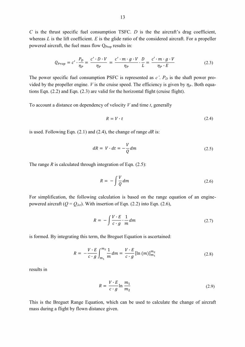
C is the thrust specific fuel consumption TSFC. D is the the aircraft’s drag coefficient,

whereas L is the lift coefficient. E is the glide ratio of the considered aircraft. For a propeller

powered aircraft, the fuel mass flow QProp results in:

(2.3)

The power specific fuel consumption PSFC is represented as c’. PD is the shaft power pro-

vided by the propeller engine. V is the cruise speed. The efficiency is given by . Both equa-

tions Eqn. (2.2) and Eqn. (2.3) are valid for the horizontal flight (cruise flight).

To account a distance on dependency of velocity V and time t, generally

(2.4)

is used. Following Eqn. (2.1) and (2.4), the change of range dR is:

(2.5)

The range R is calculated through integration of Eqn. (2.5):

(2.6)

For simplification, the following calculation is based on the range equation of an engine-

powered aircraft (Q = QJet). With insertion of Eqn. (2.2) into Eqn. (2.6),

(2.7)

is formed. By integrating this term, the Breguet Equation is ascertained:

(2.8)

results in

(2.9)

This is the Breguet Range Equation, which can be used to calculate the change of aircraft

mass during a flight by flown distance given.

14

In order to calculate the change of mass (the consumed fuel) of an aircraft for a flight with the

use of public accessible data, the Breguet Range Equation cannot be used in this form, since

data e.g. the specific fuel consumption or the glide ratio are not published by the aircraft

manufacturer. Therefore, a different procedure, which is based on the payload-range diagram

of an aircraft, is used for the fuel mass calculation.

2.2 Breguet Factor for Horizontal Flight

The data required for the Breguet Range equation relies on public non-accessible data. In

(MacDonald 2012) and (Wullbrand 2016) a procedure is demonstrated, which enables the

use of the Breguet Range equation by making use of public accessible data. To achieve this,

the Breguet Factor is adjusted.

Based on Eqn. (2.9), the Breguet Factor is written as:

(2.10)

This forms the Breguet Range Equation to:

(2.11)

A reposition of Eqn. (2.11) leads to:

(2.12)

For this calculation of the Breguet Factor, every data can be obtained from the Payload Range

Diagram.

Please note, this way of calculation is only valid for the horizontal flight.

15

2.3 Fuel Fractions

To adapt the Breguet Factor calculation not only to the horizontal flight (cruise), but to the

whole flight period including take off, climb, cruise, descend, loiter and landing, Fuel Frac-

tions are applied (MacDonald 2012).

A Fuel Fraction is a relation between the mass m2 at the end of a phase of flight and the

mass m1 at the beginning of this phase of flight.

(2.13)

The Fuel Fraction for a whole flight includes:

(2.14)

Compendious, it can be written as:

(2.15)

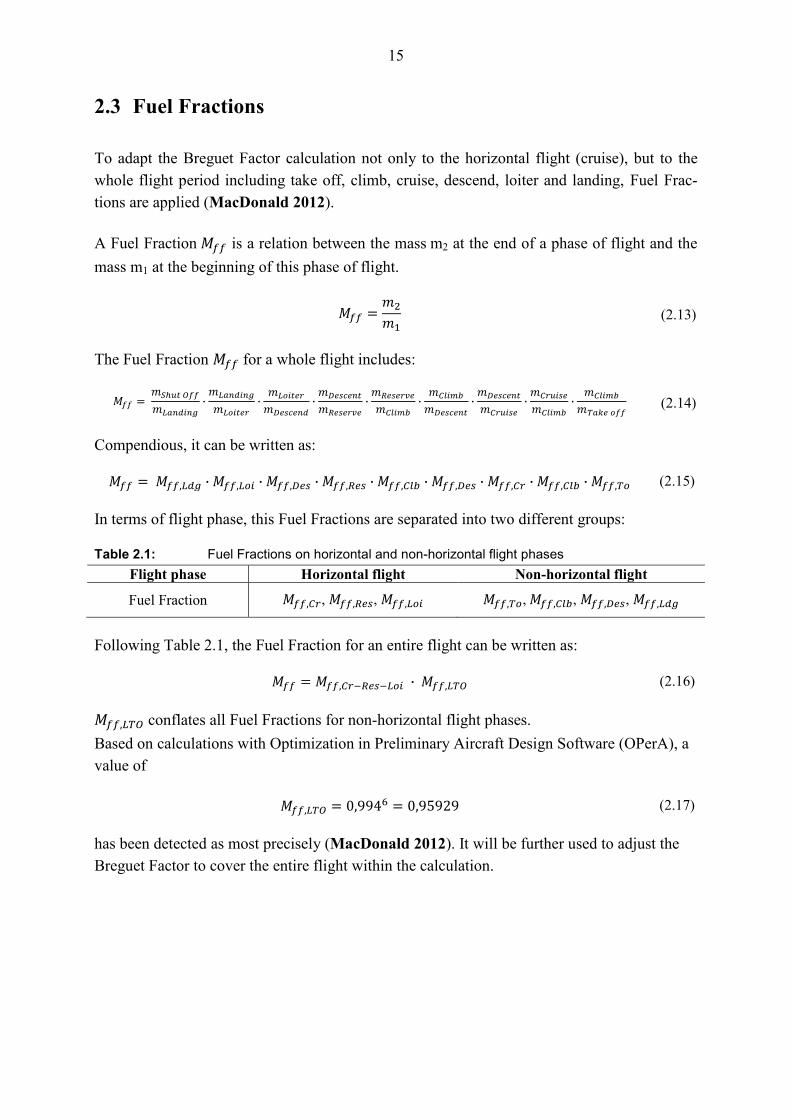
In terms of flight phase, this Fuel Fractions are separated into two different groups:

Table 2.1: Fuel Fractions on horizontal and non-horizontal flight phases

Flight phase Horizontal flight Non-horizontal flight

Fuel Fraction , , , , ,

Following Table 2.1, the Fuel Fraction for an entire flight can be written as:

(2.16)

conflates all Fuel Fractions for non-horizontal flight phases.

Based on calculations with Optimization in Preliminary Aircraft Design Software (OPerA), a

value of

(2.17)

has been detected as most precisely (MacDonald 2012). It will be further used to adjust the

Breguet Factor to cover the entire flight within the calculation.

16

2.4 Breguet Factor for Entire Flight

The Breguet Factor in Eqn. (2.12)

is limited to the horizontal flight. Since the calculation described in this chapter should cover

the entire flight including non-horizontal flight phases, the Fuel Fraction was introduced in

Chapter 2.6.

A Fuel Fraction for an entire flight can be written after reordering Eqn. (2.13) as:

(2.18)

With inclusion of Eqn. (2.16), the entire flight is depicted with:

(2.19)

In order to cover the entire flight, the mass ratio is adjusted to rely on the horizontal flight

mass ratio:

(2.20)

Following, Eqn. (2.20) is appointed to Eqn. (2.12):

(2.21)

This Breguet Factor is used for the final fuel mass calculation in this project.

17

2.5 Fuel Mass Calculation

Based on Breguet, the range can be estimated with Eqn. (2.11)

(2.22)

where m1 is the mass prior the take-off and m2 is the aircraft mass after landing. The differ-

ence between m1 and m2 can be assumed as burned fuel mass mfuel. Thus, following equation

applies (Wullbrand 2016):

(2.23)

With Eqn. (2.23) , Eqn. (2.22) can be written as:

(2.24)

In order to calculate the estimated fuel mass mfuel, the rearrangement results in:

(2.25)

This is the final equation to calculate the estimated fuel mass mfuel, depending on the range R

and the Breguet Factor B.

To highlight the dependency on the range, this equation may be used:

(2.26)

18

2.6 Aircraft Weights

The planes weight is categorized in different loads. This chapter describes the constitution of

all required aircraft weights and its components.

The Manufacturers Empty Weigh (MEW) is the structural weight of an airplane, including

the basic equipment, the engines and all required systems.

The Operation Empty Weight (OEW) includes the MEW and also customer specific perma-

nently installed equipment such as passenger seats or galleys.

The Basic Weight consist of the OEW and furthermore all operational required fluids includ-

ing hydraulics, oils and the remaining fuel, which is unusable.

The Dry Operating Weight (DOW) contains the Basic Weight and additionally the weight of

the crew, its baggage as well as water and catering for the passengers.

The Zero Fuel Weight (ZFW) adds to DOW the weight of the aircraft’s payload, including

passengers, their baggage and cargo.

Take-off Weight (TOW) is defined as the Zero Fuel Weight plus the amount of usable fuel at

the moment of take-off

The maximum fuel weight (MFW) describes the maximum possible fuel mass, which can be

carried by the aircraft. If the MFW is loaded, a payload reduction is necessary.

For the Zero Fuel Weight and the Take-off Weight, typically their respective maximum de-

rivative Maximum Zero Fuel Weight (MZFW) and Maximum Take-off Weight (MTOW) are

used.

For the Zero Fuel Weight and the Take-off Weight, their respective maximum derivative

Maximum Zero Fuel Weight (MZFW) and Maximum Take-off Weight (MTOW) are used

typically.

19

2.7 Payload Range Chart

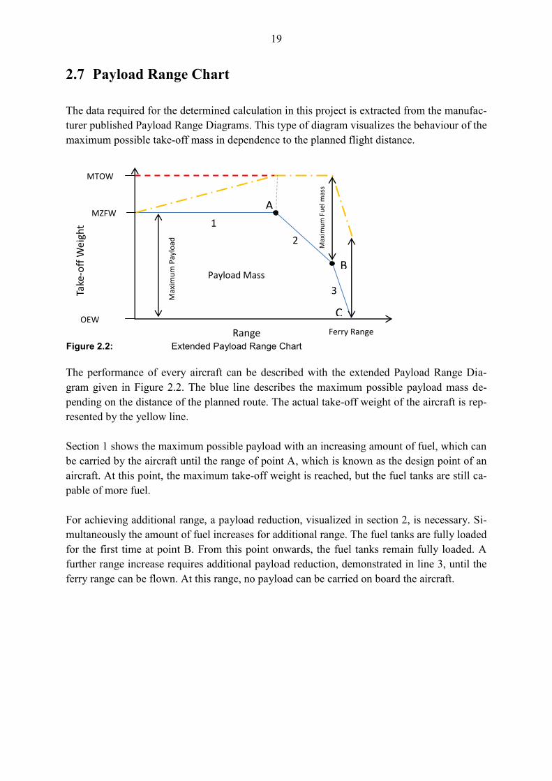
The data required for the determined calculation in this project is extracted from the manufac-

turer published Payload Range Diagrams. This type of diagram visualizes the behaviour of the

maximum possible take-off mass in dependence to the planned flight distance.

The performance of every aircraft can be described with the extended Payload Range Dia-

gram given in Figure 2.2. The blue line describes the maximum possible payload mass de-

pending on the distance of the planned route. The actual take-off weight of the aircraft is rep-

resented by the yellow line.

Section 1 shows the maximum possible payload with an increasing amount of fuel, which can

be carried by the aircraft until the range of point A, which is known as the design point of an

aircraft. At this point, the maximum take-off weight is reached, but the fuel tanks are still ca-

pable of more fuel.

For achieving additional range, a payload reduction, visualized in section 2, is necessary. Si-

multaneously the amount of fuel increases for additional range. The fuel tanks are fully loaded

for the first time at point B. From this point onwards, the fuel tanks remain fully loaded. A

further range increase requires additional payload reduction, demonstrated in line 3, until the

ferry range can be flown. At this range, no payload can be carried on board the aircraft.

Range

Take

-off

Wei

ght

OEW

MZFW

Ferry Range

1

2

3

MTOW

A

B Payload Mass

Max

imu

m F

uel

mas

s

Max

imu

m P

aylo

ad

C

Figure 2.2: Extended Payload Range Chart

20

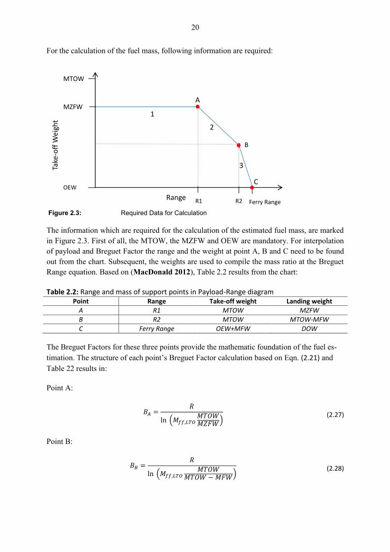
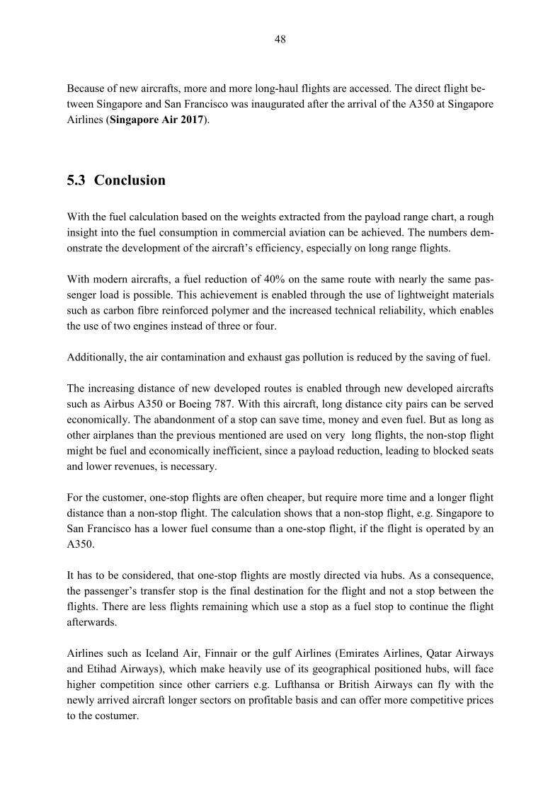
For the calculation of the fuel mass, following information are required:

Figure 2.3: Required Data for Calculation

The information which are required for the calculation of the estimated fuel mass, are marked

in Figure 2.3. First of all, the MTOW, the MZFW and OEW are mandatory. For interpolation

of payload and Breguet Factor the range and the weight at point A, B and C need to be found

out from the chart. Subsequent, the weights are used to compile the mass ratio at the Breguet

Range equation. Based on (MacDonald 2012), Table 2.2 results from the chart:

Table 2.2: Range and mass of support points in Payload-Range diagram Point Range Take-off weight Landing weight

A R1 MTOW MZFW

B R2 MTOW MTOW-MFW

C Ferry Range OEW+MFW DOW

The Breguet Factors for these three points provide the mathematic foundation of the fuel es-

timation. The structure of each point’s Breguet Factor calculation based on Eqn. (2.21) and

Table 22 results in:

Point A:

(2.27)

Point B:

(2.28)

Take

-off

Wei

ght

OEW

MZFW

MTOW

A

B

Range Ferry Range

C

2

3

1

R2 R1

21

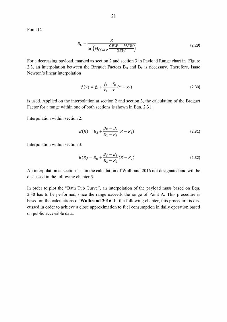
Point C:

(2.29)

For a decreasing payload, marked as section 2 and section 3 in Payload Range chart in Figure

2.3, an interpolation between the Breguet Factors BB and BC is necessary. Therefore, Isaac

Newton’s linear interpolation

(2.30)

is used. Applied on the interpolation at section 2 and section 3, the calculation of the Breguet

Factor for a range within one of both sections is shown in Eqn. 2.31:

Interpolation within section 2:

(2.31)

Interpolation within section 3:

(2.32)

An interpolation at section 1 is in the calculation of Wulbrand 2016 not designated and will be

discussed in the following chapter 3.

In order to plot the “Bath Tub Curve”, an interpolation of the payload mass based on Eqn.

2.30 has to be performed, once the range exceeds the range of Point A. This procedure is

based on the calculations of Wulbrand 2016. In the following chapter, this procedure is dis-

cussed in order to achieve a close approximation to fuel consumption in daily operation based

on public accessible data.

22

3 Examination on Fuel vs Range Diagrams

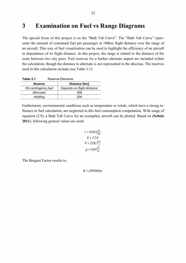
The special focus of this project is on the “Bath Tub Curve”. The “Bath Tub Curve” repre-

sents the amount of consumed fuel per passenger at 100km flight distance over the range of

an aircraft. This way of fuel visualization can be used to highlight the efficiency of an aircraft

in dependence of its flight distance. In this project, the range is related to the distance of the

route between two city pairs. Fuel reserves for a further alternate airport are included within

the calculation, though the distance to alternate is not represented in the abscissa. The reserves

used in this calculation include (see Table 3.1):

Table 3.1: Reserve Elements

Reserve Distance [km]

5% contingency fuel Depends on flight distance

Alternate 300

Holding 204

Furthermore, environmental conditions such as temperature or winds, which have a strong in-

fluence in fuel calculation, are neglected in this fuel consumption computation. With usage of

equation (2.9), a Bath Tub Curve for an exemplary aircraft can be plotted. Based on (Scholz

2011), following general values are used:

c = 0,016

E = 17,9

V = 218,7

g = 9,81

The Breguet Factor results to:

B = 24944km

23

Figure 3.1: Bath Tub Curve of an exemplary Aircraft

Figure 3.1 demonstrates a typical “Bath Tub Curve”. At shorter ranges, the fuel consumption

per passenger and range is comparatively high, since the required amount of fuel correlates

with the amount of reserves. Following, the fuel consumption per passenger and 100 km de-

creases until the minimum turning point, where the aircraft can be flown most efficient. After

this point, the consumed fuel per passenger increases, since the range requires more fuel to

even transport the additional fuel, which leads to a significantly higher take-off weight. Fur-

thermore at higher ranges, a payload reduction is required, which leads to a falling number of

passengers and results in an even higher consumption per passenger.

Based on Chapter 2, this curve and its creation will be evaluated in this chapter in order to en-

able a detailed calculation of consumed fuel based on the payload range chart. For following

calculation, the flight conditions such as flight level, temperature or cruise speed are ne-

glected, as they are not required for the fuel mass calculation as per Eqn. (2.26)

3.1 Variable Breguet Factor

As given in chapter 2.7, the characteristic of the Breguet Factor of the calculation is at a con-

stant level until the design point A, calculated with Eqn. 2.27. From point A onwards, the

Breguet Factor is interpolated between the factor at point A and point B. Same applies to the

range between point B and point C, where then Breguet Factor is interpolated between the

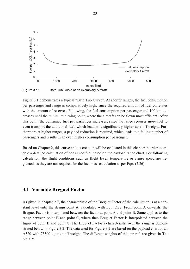
figure of point B and point C. The Breguet Factor’s characteristic over the range is demon-

strated below in Figure 3.2. The data used for Figure 3.2 are based on the payload chart of an

A320 with 73500 kg take-off weight. The different weights of this aircraft are given in Ta-

ble 3.2:

0

1

2

3

4

5

6

7

0 1000 2000 3000 4000 5000 6000

Fuel

per

10

0km

per

Pax

[kg

]

Range [km]

Fuel Consumption exemplary Aircraft

24

Table 3.2: Basic weight data A320 73.500 kg MTOW

Weight kg

MTOW 73500

DOW 42500

Max. Payload 18000

Figure 3.2: Breguet-Factor Characteristics

There are three linear sections noticeable in Figure 3.2. The first section describes the con-

stant behaviour of the Breguet Factor until the (design) point A, where the first payload re-

striction is necessary to achieve a further range. But can that factor be linear?

Based on the master thesis of MacDonald (MacDonald 2012), the replacement for the

Breguet Factor in order to extract the data out of the Payload Range chart is given in Eqn.

(2.12):

(2.12)

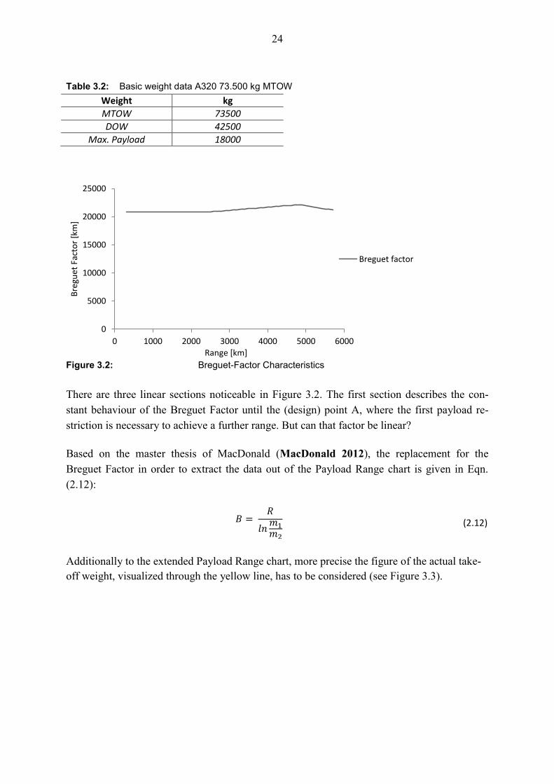
Additionally to the extended Payload Range chart, more precise the figure of the actual take-

off weight, visualized through the yellow line, has to be considered (see Figure 3.3).

0

5000

10000

15000

20000

25000

0 1000 2000 3000 4000 5000 6000

Bre

guet

Fac

tor

[km

]

Range [km]

Breguet factor

25

Figure 3.3 Figure of actual take-off weight

Because of an increasing take-off weight, visualized through the yellow line, the mass ratio

in the Breguet Factor cannot be assumed as linear. Hence, the use of a constant amount for

the Breguet Factor at the first section until the point A is inadequate.

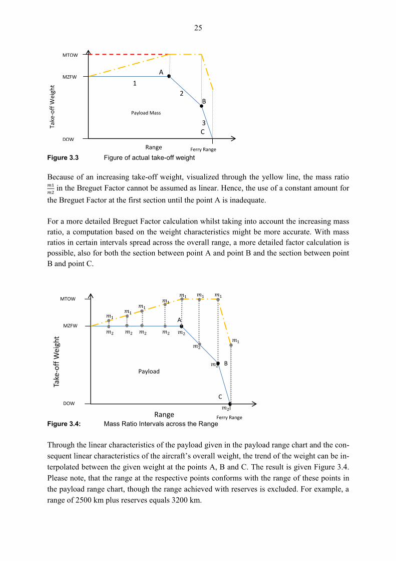
For a more detailed Breguet Factor calculation whilst taking into account the increasing mass

ratio, a computation based on the weight characteristics might be more accurate. With mass

ratios in certain intervals spread across the overall range, a more detailed factor calculation is

possible, also for both the section between point A and point B and the section between point

B and point C.

Figure 3.4: Mass Ratio Intervals across the Range

Through the linear characteristics of the payload given in the payload range chart and the con-

sequent linear characteristics of the aircraft’s overall weight, the trend of the weight can be in-

terpolated between the given weight at the points A, B and C. The result is given Figure 3.4.

Please note, that the range at the respective points conforms with the range of these points in

the payload range chart, though the range achieved with reserves is excluded. For example, a

range of 2500 km plus reserves equals 3200 km.

Range

Take

-off

Wei

ght

DOW

MZFW

Ferry Range

1

2

3

MTOW

A

B

Payload Mass

C

Range

Take

-off

Wei

ght

DOW

MZFW

Ferry Range

MTOW

A

B

Payload Mass

C

26

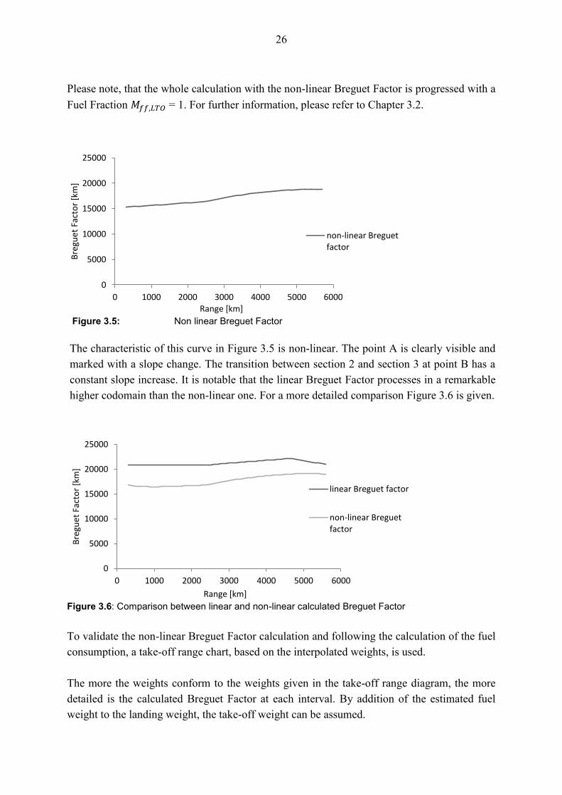
Please note, that the whole calculation with the non-linear Breguet Factor is progressed with a

Fuel Fraction = 1. For further information, please refer to Chapter 3.2.

Figure 3.5: Non linear Breguet Factor

The characteristic of this curve in Figure 3.5 is non-linear. The point A is clearly visible and

marked with a slope change. The transition between section 2 and section 3 at point B has a

constant slope increase. It is notable that the linear Breguet Factor processes in a remarkable

higher codomain than the non-linear one. For a more detailed comparison Figure 3.6 is given.

Figure 3.6: Comparison between linear and non-linear calculated Breguet Factor

To validate the non-linear Breguet Factor calculation and following the calculation of the fuel

consumption, a take-off range chart, based on the interpolated weights, is used.

The more the weights conform to the weights given in the take-off range diagram, the more

detailed is the calculated Breguet Factor at each interval. By addition of the estimated fuel

weight to the landing weight, the take-off weight can be assumed.

0

5000

10000

15000

20000

25000

0 1000 2000 3000 4000 5000 6000

Bre

guet

Fac

tor

[km

]

Range [km]

non-linear Breguet factor

0

5000

10000

15000

20000

25000

0 1000 2000 3000 4000 5000 6000

Bre

guet

Fac

tor

[km

]

Range [km]

linear Breguet factor

non-linear Breguet factor

27

The landing weight is extracted the payload range chart or can be calculated via the addition

of the shown payload weight and the constant OEW. This amount will be compared to the

take-off weight given by the payload range chart. The addressed points for calculation are the

points A, B and C. The take-off weight at the respective point is demonstrated in Table 3.3:

Table 3.3: Take-off Weights at respective appoints in Payload Range Chart

Point Take-off weight

A MTOW

B MTOW

C OEW+MFW

By usage of interpolation for each section between the named points, the actual take-off

weight can be calculated for every range.

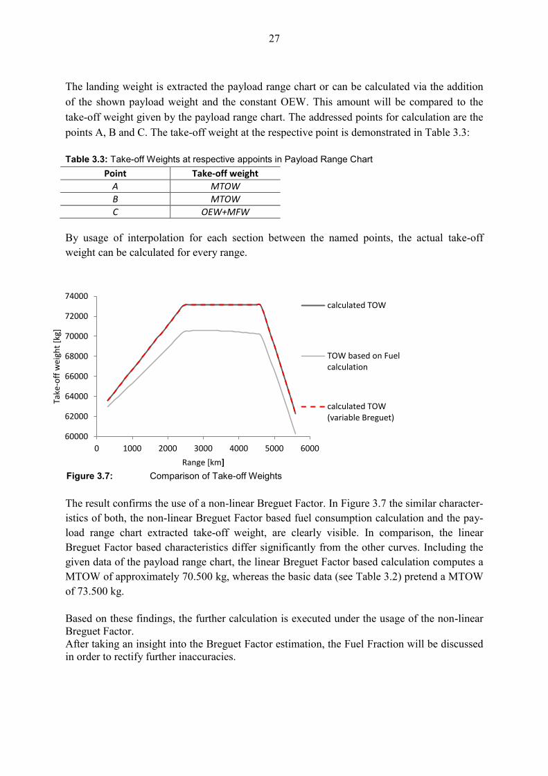
The result confirms the use of a non-linear Breguet Factor. In Figure 3.7 the similar character-

istics of both, the non-linear Breguet Factor based fuel consumption calculation and the pay-

load range chart extracted take-off weight, are clearly visible. In comparison, the linear

Breguet Factor based characteristics differ significantly from the other curves. Including the

given data of the payload range chart, the linear Breguet Factor based calculation computes a

MTOW of approximately 70.500 kg, whereas the basic data (see Table 3.2) pretend a MTOW

of 73.500 kg.

Based on these findings, the further calculation is executed under the usage of the non-linear

Breguet Factor.

After taking an insight into the Breguet Factor estimation, the Fuel Fraction will be discussed

in order to rectify further inaccuracies.

60000

62000

64000

66000

68000

70000

72000

74000

0 1000 2000 3000 4000 5000 6000

Take

-off

wei

ght

[kg]

Range [km]

calculated TOW

TOW based on Fuel calculation

calculated TOW (variable Breguet)

Figure 3.7: Comparison of Take-off Weights

28

3.2 Fuel Fraction

The Fuel Fraction was implemented to adapt the Breguet Factor, which was primary used for

calculation at the horizontal flight phase, to the whole flight, including take-off, climb, de-

scent or landing phase. It is demonstrated in Eqn. ((2.21):

(2.21)

The Fuel Fraction Mff,LTO has a constant value as given in Eqn. (2.17):

(2.17)

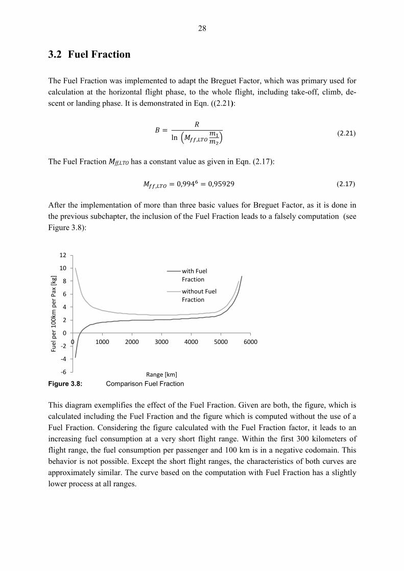
After the implementation of more than three basic values for Breguet Factor, as it is done in

the previous subchapter, the inclusion of the Fuel Fraction leads to a falsely computation (see

Figure 3.8):

Figure 3.8: Comparison Fuel Fraction

This diagram exemplifies the effect of the Fuel Fraction. Given are both, the figure, which is

calculated including the Fuel Fraction and the figure which is computed without the use of a

Fuel Fraction. Considering the figure calculated with the Fuel Fraction factor, it leads to an

increasing fuel consumption at a very short flight range. Within the first 300 kilometers of

flight range, the fuel consumption per passenger and 100 km is in a negative codomain. This

behavior is not possible. Except the short flight ranges, the characteristics of both curves are

approximately similar. The curve based on the computation with Fuel Fraction has a slightly

lower process at all ranges.

-6

-4

-2

0

2

4

6

8

10

12

0 1000 2000 3000 4000 5000 6000

Fuel

per

10

0km

per

Pax

[kg

]

Range [km]

with Fuel Fraction

without Fuel Fraction

29

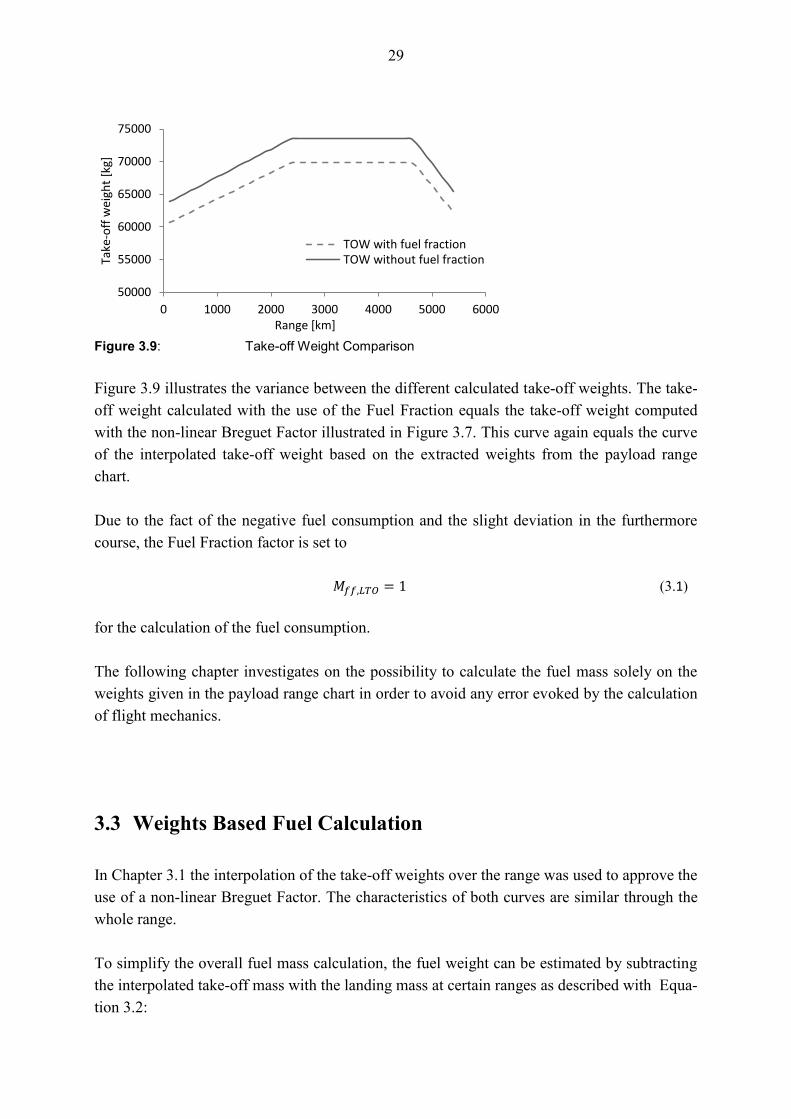
Figure 3.9: Take-off Weight Comparison

Figure 3.9 illustrates the variance between the different calculated take-off weights. The take-

off weight calculated with the use of the Fuel Fraction equals the take-off weight computed

with the non-linear Breguet Factor illustrated in Figure 3.7. This curve again equals the curve

of the interpolated take-off weight based on the extracted weights from the payload range

chart.

Due to the fact of the negative fuel consumption and the slight deviation in the furthermore

course, the Fuel Fraction factor is set to

(3.1)

for the calculation of the fuel consumption.

The following chapter investigates on the possibility to calculate the fuel mass solely on the

weights given in the payload range chart in order to avoid any error evoked by the calculation

of flight mechanics.

3.3 Weights Based Fuel Calculation

In Chapter 3.1 the interpolation of the take-off weights over the range was used to approve the

use of a non-linear Breguet Factor. The characteristics of both curves are similar through the

whole range.

To simplify the overall fuel mass calculation, the fuel weight can be estimated by subtracting

the interpolated take-off mass with the landing mass at certain ranges as described with Equa-

tion 3.2:

50000

55000

60000

65000

70000

75000

0 1000 2000 3000 4000 5000 6000

Take

-off

wei

ght

[kg]

Range [km]

TOW with fuel fraction TOW without fuel fraction

30

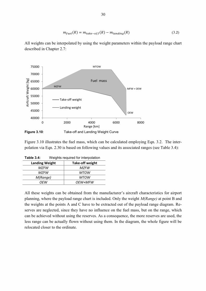
(3.2)

All weights can be interpolated by using the weight parameters within the payload range chart

described in Chapter 2.7:

Figure 3.10: Take-off and Landing Weight Curve

Figure 3.10 illustrates the fuel mass, which can be calculated employing Eqn. 3.2. The inter-

polation via Eqn. 2.30 is based on following values and its associated ranges (see Table 3.4):

Table 3.4: Weights required for interpolation

Landing Weight Take-off weight

MZFW MZFW

MZFW MTOW

M(Range) MTOW

OEW OEW+MFW

All these weights can be obtained from the manufacturer’s aircraft characteristics for airport

planning, where the payload range chart is included. Only the weight M(Range) at point B and

the weights at the points A and C have to be extracted out of the payload range diagram. Re-

serves are neglected, since they have no influence on the fuel mass, but on the range, which

can be achieved without using the reserves. As a consequence, the more reserves are used, the

less range can be actually flown without using them. In the diagram, the whole figure will be

relocated closer to the ordinate.

40000

45000

50000

55000

60000

65000

70000

75000

0 2000 4000 6000 8000

Air

fcra

ft W

eigh

t [k

g]

Range [km]

Take-off weight

Landing weight

MTOW

MZFW

OEW

MFW + OEW

Fuel mass

31

3.4 Further Investigation and Conclusion

The overall validation of this data with real data is due to the fact of a strictly secrecy on be-

half of the aircraft manufacturer not possible. Therefore, this examination bases on the expec-

tations of the known flight mechanics. In this chapter, two methods for a more detailed fuel

calculation are demonstrated and closer investigated. The foundation of the whole calculation

is given by the project of Wullbrand (Wullbrand 2016).

In Chapter 3.3, a new method is provided. This method spares the flight mechanics and bases

solely on the weights at different flight phases.

By adapting a more detailed Breguet Factor, the calculation becomes more detailed. This

could be proofed with the actual fuel mass required for the flight. With a linear Breguet Fac-

tor, the fuel weights are clearly below the maximum possible fuel weight as demonstrated in

Figure 3.7.

The removal of the Fuel Fraction is a necessary consequence when using the detailed, not lin-

ear Breguet Factor. This leads to a more realistic fuel consumption behaviour at shorter ranges

(see Figure 3.8) and a more detailed fuel mass, too (see Figure 3.9).

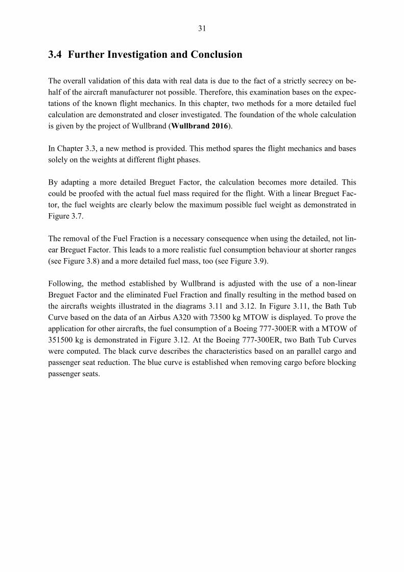
Following, the method established by Wullbrand is adjusted with the use of a non-linear

Breguet Factor and the eliminated Fuel Fraction and finally resulting in the method based on

the aircrafts weights illustrated in the diagrams 3.11 and 3.12. In Figure 3.11, the Bath Tub

Curve based on the data of an Airbus A320 with 73500 kg MTOW is displayed. To prove the

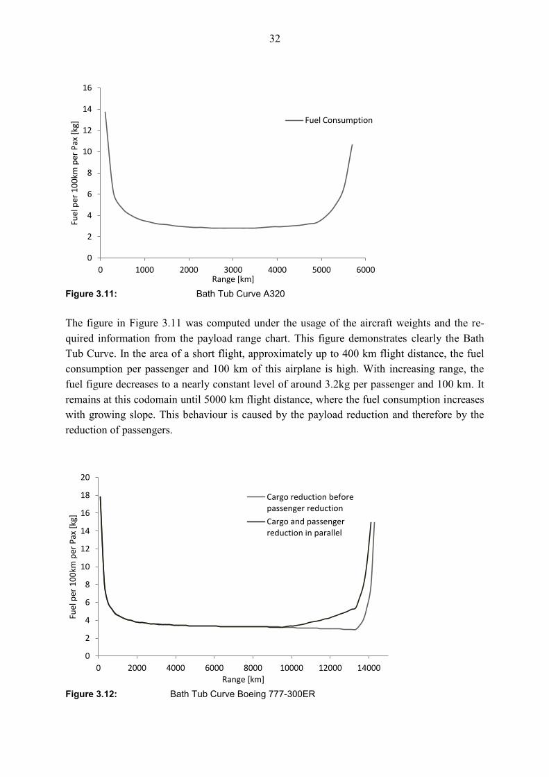
application for other aircrafts, the fuel consumption of a Boeing 777-300ER with a MTOW of

351500 kg is demonstrated in Figure 3.12. At the Boeing 777-300ER, two Bath Tub Curves

were computed. The black curve describes the characteristics based on an parallel cargo and

passenger seat reduction. The blue curve is established when removing cargo before blocking

passenger seats.

32

Figure 3.11: Bath Tub Curve A320

The figure in Figure 3.11 was computed under the usage of the aircraft weights and the re-

quired information from the payload range chart. This figure demonstrates clearly the Bath

Tub Curve. In the area of a short flight, approximately up to 400 km flight distance, the fuel

consumption per passenger and 100 km of this airplane is high. With increasing range, the

fuel figure decreases to a nearly constant level of around 3.2kg per passenger and 100 km. It

remains at this codomain until 5000 km flight distance, where the fuel consumption increases

with growing slope. This behaviour is caused by the payload reduction and therefore by the

reduction of passengers.

Figure 3.12: Bath Tub Curve Boeing 777-300ER

0

2

4

6

8

10

12

14

16

0 1000 2000 3000 4000 5000 6000

Fuel

per

10

0km

per

Pax

[kg

]

Range [km]

Fuel Consumption

0

2

4

6

8

10

12

14

16

18

20

0 2000 4000 6000 8000 10000 12000 14000

Fuel

per

10

0km

per

Pax

[kg

]

Range [km]

Cargo reduction before passenger reduction

Cargo and passenger reduction in parallel

33

The Bath Tub Curves of the Boeing 777-300ER given in Figure 3.12 present an overall simi-

lar behaviour as the Bath Tub Curve of an Airbus A320. The high fuel consumption per pas-

senger and 100 km flight distance at short ranges are followed by an approximately constant

figure until 10000 kilometres. It is notable, that at this range a decrease of fuel consumption

takes place at the blue curve. This occurs, since a payload reduction is necessary. This pay-

load reduction has no effect on the number of transported passengers. The calculation implies

the removal of all belly cargo before passenger numbers are reduced.

The black curve demonstrates a parallel decrease of belly cargo and number of passengers.

Subsequently, the amount of fuel burned per passenger and 100 km increases at this phase of

flight.

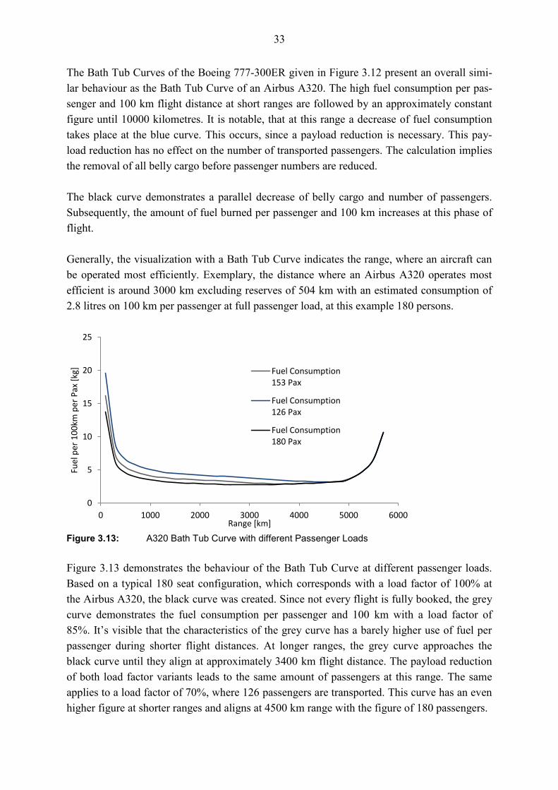
Generally, the visualization with a Bath Tub Curve indicates the range, where an aircraft can

be operated most efficiently. Exemplary, the distance where an Airbus A320 operates most

efficient is around 3000 km excluding reserves of 504 km with an estimated consumption of

2.8 litres on 100 km per passenger at full passenger load, at this example 180 persons.

Figure 3.13: A320 Bath Tub Curve with different Passenger Loads

Figure 3.13 demonstrates the behaviour of the Bath Tub Curve at different passenger loads.

Based on a typical 180 seat configuration, which corresponds with a load factor of 100% at

the Airbus A320, the black curve was created. Since not every flight is fully booked, the grey

curve demonstrates the fuel consumption per passenger and 100 km with a load factor of

85%. It’s visible that the characteristics of the grey curve has a barely higher use of fuel per

passenger during shorter flight distances. At longer ranges, the grey curve approaches the

black curve until they align at approximately 3400 km flight distance. The payload reduction

of both load factor variants leads to the same amount of passengers at this range. The same

applies to a load factor of 70%, where 126 passengers are transported. This curve has an even

higher figure at shorter ranges and aligns at 4500 km range with the figure of 180 passengers.

0

5

10

15

20

25

0 1000 2000 3000 4000 5000 6000

Fuel

per

10

0km

per

Pax

[kg

]

Range [km]

Fuel Consumption 153 Pax



34

Please be aware, that the calculation does not adjust the payload weight at take off with a re-

duced passenger number. This demonstrates, although for the example with a load factor of

70% is given, the payload is still at its maximum, for example because more cargo is carried.

A calculation based on varying payload weights is not possible, since the payload range dia-

gram, on which this calculation is based, does not contain information about different pay-

loads at smaller load factors.

As mentioned before, an alignment with real data is not possible. With the computation, a

roughly estimation of the fuel consumption of a certain aircraft over the range is provided.

This computation neglects the flight mechanics, for example the flight level which is flown,

the speed or any step climbs, which have an impact on the fuel consumption.

Furthermore, the environmental conditions are not involved into the calculation. Any head-

winds, tailwinds or other atmospheric impacts, which highly influence the fuel consumption

at every flight, are not taken into consideration. This issue has to be regarded when using this

calculation.

Summarizing, this calculation based on the payload range chart provides a basic estimation of

the fuel consumption of an aircraft.

In the next chapter a detailed view on the various visualizations of the fuel consumption is

made.

35

4 View on Different Fuel Consumption Visualiza-

tions

This chapter deals with the different ways of the representation of an aircraft´s fuel consump-

tion. Three more kinds of charts will be explained and later compared with the previous dis-

cussed Bath Tub Curve. The calculation for each data displayed in the charts is based on the

fundamentals in Chapter 2 and the analysis in Chapter 3.

4.1 Fuel vs Range Chart

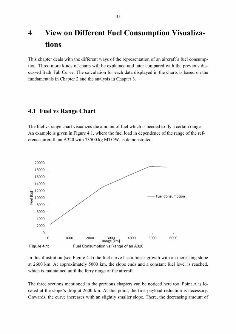
The fuel vs range chart visualizes the amount of fuel which is needed to fly a certain range.

An example is given in Figure 4.1, where the fuel load in dependence of the range of the ref-

erence aircraft, an A320 with 73500 kg MTOW, is demonstrated.

Figure 4.1: Fuel Consumption vs Range of an A320

In this illustration (see Figure 4.1) the fuel curve has a linear growth with an increasing slope

at 2600 km. At approximately 5000 km, the slope ends and a constant fuel level is reached,

which is maintained until the ferry range of the aircraft.

The three sections mentioned in the previous chapters can be noticed here too. Point A is lo-

cated at the slope’s drop at 2600 km. At this point, the first payload reduction is necessary.

Onwards, the curve increases with an slightly smaller slope. There, the decreasing amount of

0

2000

4000

6000

8000

10000

12000

14000

16000

18000

20000

0 1000 2000 3000 4000 5000 6000

Fuel

[kg

]

Range [km]

Fuel Consumption

36

payload is responsible for the smaller increase of required fuel. Once the curve reaches point

B, the fuel capability of the aircraft is completely in use. Hence, the amount of fuel cannot be

increased anymore and remains on a constant level of approx. 18730 kg for this example.

Point C can be found at the aircraft´s ferry range at 5800 km at the end of the curve.

In the following subchapter, the mass per range vs range chart will be further explained.

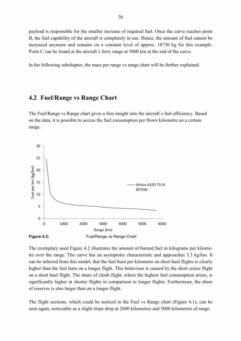
4.2 Fuel/Range vs Range Chart

The Fuel/Range vs Range chart gives a first insight into the aircraft´s fuel efficiency. Based

on the data, it is possible to access the fuel consumption per flown kilometre on a certain

range.

Figure 4.2: Fuel/Range vs Range Chart

The exemplary used Figure 4.2 illustrates the amount of burned fuel in kilograms per kilome-

tre over the range. The curve has an asymptotic characteristic and approaches 3.3 kg/km. It

can be inferred from this model, that the fuel burn per kilometre on short haul flights is clearly

higher than the fuel burn on a longer flight. This behaviour is caused by the short cruise flight

on a short haul flight. The share of climb flight, where the highest fuel consumption arises, is

significantly higher at shorter flights in comparison to longer flights. Furthermore, the share

of reserves is also larger than on a longer flight.

The flight sections, which could be noticed in the Fuel vs Range chart (Figure 4.1), can be

seen again, noticeable as a slight slope drop at 2600 kilometres and 5000 kilometres of range.

0

5

10

15

20

25

30

0 1000 2000 3000 4000 5000 6000

Fuel

per

km

[kg

/km

]

Range [km]

Airbus A320 73.5t MTOW

37

This form of visualization demonstrates a growing efficiency at longer flown flight distances.

The lower fuel consumption on longer flights takes place due the shrinking share of fuel re-

serves. The effect on longer ranges, where fuel has be carried to carry fuel and its following

inefficiency is not visible in this kind of illustration, since only absolute values are used,

which do not imply the payload reduction at longer distances.

The growing inefficiency in terms of payload is demonstrated in the next chapter.

4.3 Fuel/Payload vs Range Chart

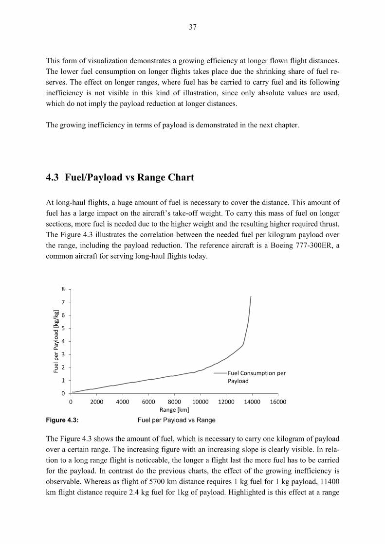
At long-haul flights, a huge amount of fuel is necessary to cover the distance. This amount of

fuel has a large impact on the aircraft’s take-off weight. To carry this mass of fuel on longer

sections, more fuel is needed due to the higher weight and the resulting higher required thrust.

The Figure 4.3 illustrates the correlation between the needed fuel per kilogram payload over

the range, including the payload reduction. The reference aircraft is a Boeing 777-300ER, a

common aircraft for serving long-haul flights today.

Figure 4.3: Fuel per Payload vs Range

The Figure 4.3 shows the amount of fuel, which is necessary to carry one kilogram of payload

over a certain range. The increasing figure with an increasing slope is clearly visible. In rela-

tion to a long range flight is noticeable, the longer a flight last the more fuel has to be carried

for the payload. In contrast do the previous charts, the effect of the growing inefficiency is

observable. Whereas as flight of 5700 km distance requires 1 kg fuel for 1 kg payload, 11400

km flight distance require 2.4 kg fuel for 1kg of payload. Highlighted is this effect at a range

0

1

2

3

4

5

6

7

8

0 2000 4000 6000 8000 10000 12000 14000 16000

Fuel

per

Pay

load

[kg

/kg]

Range [km]

Fuel Consumption per Payload

38

of 13900 km, where 7.45 kg of fuel are needed for every kilogram of payload. This effect may

be explained through the fuel, which is required to transport fuel to achieve a longer range.

This effect is visible at the Bath Tub Curve. The longer the flight, the higher is the consump-

tion of fuel per passenger and 100 km.

The next chapter deals with the relation of all diagrams represented in the previous chapters.

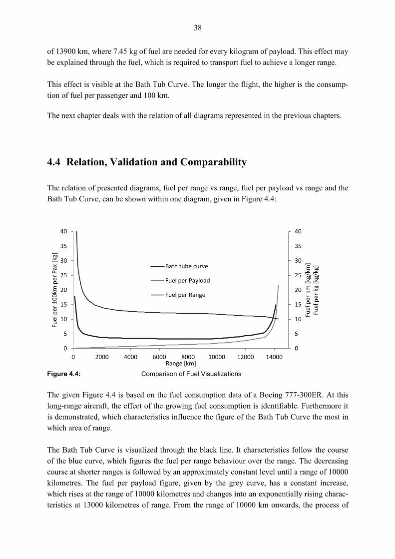
4.4 Relation, Validation and Comparability

The relation of presented diagrams, fuel per range vs range, fuel per payload vs range and the

Bath Tub Curve, can be shown within one diagram, given in Figure 4.4:

Figure 4.4: Comparison of Fuel Visualizations

The given Figure 4.4 is based on the fuel consumption data of a Boeing 777-300ER. At this

long-range aircraft, the effect of the growing fuel consumption is identifiable. Furthermore it

is demonstrated, which characteristics influence the figure of the Bath Tub Curve the most in

which area of range.

The Bath Tub Curve is visualized through the black line. It characteristics follow the course

of the blue curve, which figures the fuel per range behaviour over the range. The decreasing

course at shorter ranges is followed by an approximately constant level until a range of 10000

kilometres. The fuel per payload figure, given by the grey curve, has a constant increase,

which rises at the range of 10000 kilometres and changes into an exponentially rising charac-

teristics at 13000 kilometres of range. From the range of 10000 km onwards, the process of

0

5

10

15

20

25

30

35

40

0

5

10

15

20

25

30

35

40

0 2000 4000 6000 8000 10000 12000 14000

Fuel

per

km

[kg

/km

] Fu

el p

er k

g [k

g/kg

]

Fuel

per

10

0km

per

Pax

[kg

]

Range [km]

Bath tube curve

Fuel per Payload

Fuel per Range

39

the Bath Tub Curve is orientated at the fuel per payload figure, whereas the fuel per range

figure is decreasing slightly.

The Bath Tub Curve contains both, the inefficiency of an aircraft at a very short flight dis-

tance and the growing inefficiency at longer ranges of an aircraft. Based on this curve, the

area, which covers the range where an aircraft can be operated most efficiently, can be found.

In next chapter, today´s aircraft operation will be investigated under the consideration of the

Bath Tub Curve, regarding the question whether to fly non-stop or one-stop.

40

5 Fuel Consumption in Aircraft Operation

In today’s aircraft operation, many more long-haul routes are inaugurated every year. Due to

the availability of new generation aircraft as the Boeing 787 or the Airbus A350 long-haul

routes become more and more viable, since this aircrafts fly very fuel efficient in comparison

to aircrafts of the last decade. This chapter will take a closer look at the aircraft operated to-

day and its fuel consumption in comparison to aircraft of earlier days. Furthermore, a primary

investigation is done about the question whether a route should be flown non-stop or one stop

under the ecological and economical point of view.

The first chapter will compare older aircraft and newer aircraft to demonstrate the decreased

fuel consumption. The second chapter evaluates between a non-stop and one-stop long-haul

flight. The calculation used in this chapter is based on the perceptions of the previous chapters

and the Excel tool described in chapter 6.

5.1 Fuel Consumption of modern Aircraft

In order to demonstrate the growing efficiency of new aircrafts, a comparison between the

1980s built Boeing 747-200B, with the 2005 introduced Boeing 777-300ER and the upcom-

ing Airbus A350-1000 is done. This three aircraft represent roughly the same seat capacity.

For a more detailed analysis, the Hong Kong based airline Cathay Pacific is chosen to obtain

seat capacity data of a real airline. This airline has flown the 747-200B (Frequent 2012) and

is flying the 777-300ER (Cathay 2017). By 2018, Cathay Pacific will receive the largest ver-

sion of the Airbus A350, the -1000. The flight, on which the fuel data are compared, is a real

flight, too. CX 289 departs from Hong Kong Chek Lap Kok Airport to Frankfurt Airport and

covers a great circle distance of 9166 km.

The aircraft specifications required for the fuel calculation are demonstrated in Table 5.1:

41

Table 5.1: Aircraft Specifications

Data Boeing 747-200B Boeing 777-300ER Airbus A350-1000

MTOW 371900 kg 351535 kg 308000 kg

MZFW 238780 kg 237682 kg 220000 kg

OEW 174970 kg 167829 kg 155500 kg

MFW 159250 kg 145538 kg 122460 kg

Max. Payload 67360 kg 69853 kg 64500 kg

Range at point A 8148 km 10556 km 10000 km

Payload at point B 33910 kg 38671 kg 28000 kg

Range at point B 10741 km 14466 km 16000 km

Range at point C 13020 km 15742 km 18000 km

Seat capacity 363 340 340 (estimated)

The seat capacity of the Cathay Pacific customized A350-1000 is not published yet, due the

delivery in 2018. Therefore, the number is estimated by the author and simplifies the com-

parison between the Boeing 777-300ER and the Airbus A350-1000. Following the Airbus

document, a 3-class seating is available with 366 seats. Cathay Pacific uses a 4-class configu-

ration, thus the seat capacity is with 340 seats slightly below the Airbus standard.

For calculation, the international reserve (see Chapter 6) is used, which results in a 10624 km

possible flight distance including reserves. Furthermore, the cargo was reduced before seats

were blocked.

The calculation results in Table 5.2 relating to the 9166 km long trip:

Table 5.2: Fuel Consumption Flight CX289 Hong Kong - Frankfurt

Consumption Boeing 747-200B Boeing 777-300ER Airbus A350-1000

Overall Fuel 161671 kg 114213 kg 91796 kg

Change - -29.3 % -19.6 %

Change 747 – A350 - - -43.2 %

Fuel per Pax and

100km 4.96 kg 3.65 kg 2.93 kg

Change - -26.5 % -19.7 %

Change 747 – A350 - - -40.3 %

Fuel per kilogram Pay-

load 4.56 kg 1.65 kg 1.51 kg

Change - -63.8 % -8.4 %

Change 747 – A350 - - -66.8 %

42

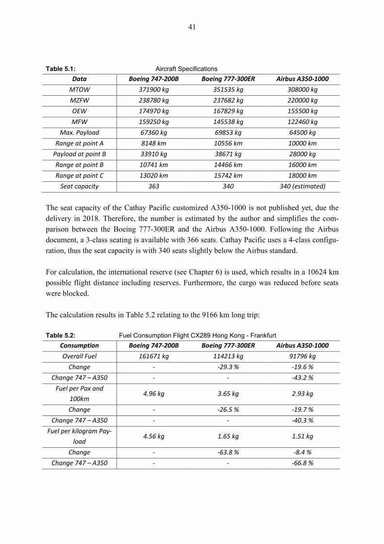
It is clearly visible, that the two engined aircraft Boeing 777-300ER and Airbus A350-1000

consume obvious less fuel then the four engine powered Boeing 747-200B. Figure 5.1 illus-

trates the different amounts of fuel, which are necessary to operate the flight between Hong

Kong and Frankfurt.

Figure 5.1: Trip Fuel CX289

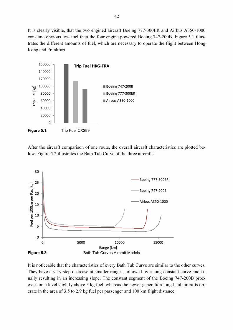
After the aircraft comparison of one route, the overall aircraft characteristics are plotted be-

low. Figure 5.2 illustrates the Bath Tub Curve of the three aircrafts:

Figure 5.2: Bath Tub Curves Aircraft Models

It is noticeable that the characteristics of every Bath Tub Curve are similar to the other curves.

They have a very step decrease at smaller ranges, followed by a long constant curve and fi-

nally resulting in an increasing slope. The constant segment of the Boeing 747-200B proc-

esses on a level slightly above 5 kg fuel, whereas the newer generation long-haul aircrafts op-

erate in the area of 3.5 to 2.9 kg fuel per passenger and 100 km flight distance.

0

20000

40000

60000

80000

100000

120000

140000

160000

Trip

Fu

el [

kg]

Trip Fuel HKG-FRA

Boeing 747-200B

Boeing 777-300ER

Airbus A350-1000

0

5

10

15

20

25

30

0 5000 10000 15000

Fuel

per

10

0km

per

Pax

[kg

]

Range [km]

Boeing 777-300ER

Boeing 747-200B

Airbus A350-1000

43

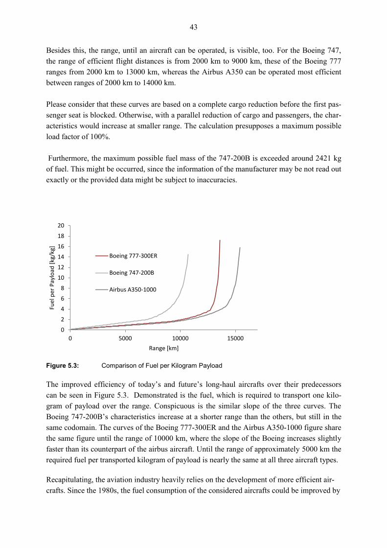
Besides this, the range, until an aircraft can be operated, is visible, too. For the Boeing 747,

the range of efficient flight distances is from 2000 km to 9000 km, these of the Boeing 777

ranges from 2000 km to 13000 km, whereas the Airbus A350 can be operated most efficient

between ranges of 2000 km to 14000 km.

Please consider that these curves are based on a complete cargo reduction before the first pas-

senger seat is blocked. Otherwise, with a parallel reduction of cargo and passengers, the char-

acteristics would increase at smaller range. The calculation presupposes a maximum possible

load factor of 100%.

Furthermore, the maximum possible fuel mass of the 747-200B is exceeded around 2421 kg

of fuel. This might be occurred, since the information of the manufacturer may be not read out

exactly or the provided data might be subject to inaccuracies.

Figure 5.3: Comparison of Fuel per Kilogram Payload

The improved efficiency of today’s and future’s long-haul aircrafts over their predecessors

can be seen in Figure 5.3. Demonstrated is the fuel, which is required to transport one kilo-

gram of payload over the range. Conspicuous is the similar slope of the three curves. The

Boeing 747-200B’s characteristics increase at a shorter range than the others, but still in the

same codomain. The curves of the Boeing 777-300ER and the Airbus A350-1000 figure share

the same figure until the range of 10000 km, where the slope of the Boeing increases slightly

faster than its counterpart of the airbus aircraft. Until the range of approximately 5000 km the

required fuel per transported kilogram of payload is nearly the same at all three aircraft types.

Recapitulating, the aviation industry heavily relies on the development of more efficient air-

crafts. Since the 1980s, the fuel consumption of the considered aircrafts could be improved by

0

2

4

6

8

10

12

14

16

18

20

0 5000 10000 15000

Fuel

per

Pay

load

[kg

/kg]

Range [km]

Boeing 777-300ER

Boeing 747-200B

Airbus A350-1000

44

more than 40% .This improvement can only be achieved on longer flight sectors. At shorter

flight sectors, the improvement is obvious smaller.

In relation to the fuel consumption per passenger, the consumption on shorter sectors is not as

much improved as on longer flights with the usage of new generation aircraft.

Generally, aircrafts of today consume distinctly less fuel than aircraft of the previous century

and enable airlines to offer more direct long-haul flights on economical viable basis.

Next chapter investigates on the rising numbers of direct flights and compares this behaviour

with the model of connecting passengers on an airport hub with one-stop journeys.

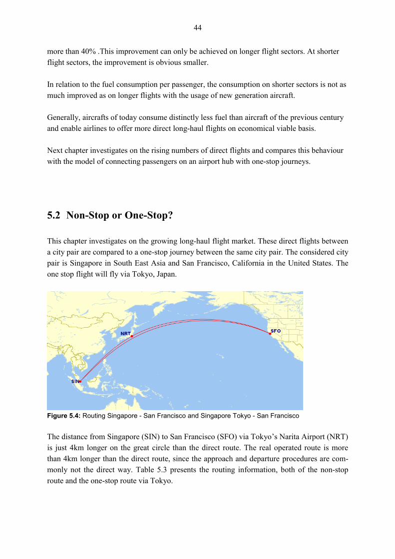
5.2 Non-Stop or One-Stop?

This chapter investigates on the growing long-haul flight market. These direct flights between

a city pair are compared to a one-stop journey between the same city pair. The considered city

pair is Singapore in South East Asia and San Francisco, California in the United States. The

one stop flight will fly via Tokyo, Japan.

Figure 5.4: Routing Singapore - San Francisco and Singapore Tokyo - San Francisco

The distance from Singapore (SIN) to San Francisco (SFO) via Tokyo’s Narita Airport (NRT)

is just 4km longer on the great circle than the direct route. The real operated route is more

than 4km longer than the direct route, since the approach and departure procedures are com-

monly not the direct way. Table 5.3 presents the routing information, both of the non-stop

route and the one-stop route via Tokyo.

45

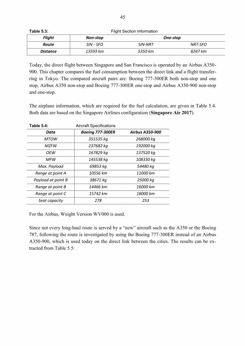
Table 5.3: Flight Section Information

Flight Non-stop One-stop

Route SIN - SFO SIN-NRT NRT-SFO

Distance 13593 km 5350 km 8247 km

Today, the direct flight between Singapore and San Francisco is operated by an Airbus A350-

900. This chapter compares the fuel consumption between the direct link and a flight transfer-

ring in Tokyo. The compared aircraft pairs are: Boeing 777-300ER both non-stop and one

stop, Airbus A350 non-stop and Boeing 777-300ER one-stop and Airbus A350-900 non-stop

and one-stop.

The airplane information, which are required for the fuel calculation, are given in Table 5.4.

Both data are based on the Singapore Airlines configuration (Singapore Air 2017).

Table 5.4: Aircraft Specifications

Data Boeing 777-300ER Airbus A350-900

MTOW 351535 kg 268000 kg

MZFW 237682 kg 192000 kg

OEW 167829 kg 137520 kg

MFW 145538 kg 108330 kg

Max. Payload 69853 kg 54480 kg

Range at point A 10556 km 11000 km

Payload at point B 38671 kg 25000 kg

Range at point B 14466 km 16000 km

Range at point C 15742 km 18000 km

Seat capacity 278 253

For the Airbus, Weight Version WV000 is used.

Since not every long-haul route is served by a “new” aircraft such as the A350 or the Boeing

787, following the route is investigated by using the Boeing 777-300ER instead of an Airbus

A350-900, which is used today on the direct link between the cities. The results can be ex-

tracted from Table 5.5:

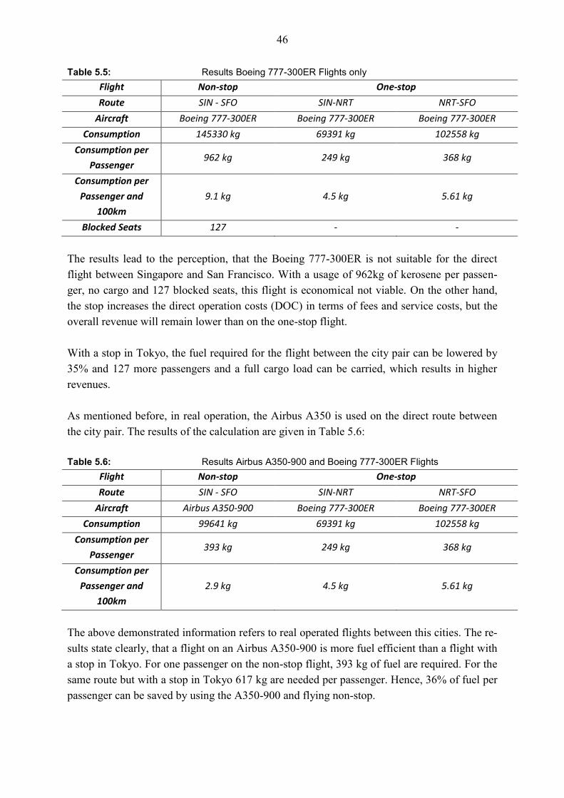
46

Table 5.5: Results Boeing 777-300ER Flights only



Aircraft Boeing 777-300ER Boeing 777-300ER Boeing 777-300ER

Consumption 145330 kg 69391 kg 102558 kg

Consumption per

Passenger 962 kg 249 kg 368 kg

Consumption per

Passenger and

100km

9.1 kg 4.5 kg 5.61 kg

Blocked Seats 127 - -

The results lead to the perception, that the Boeing 777-300ER is not suitable for the direct

flight between Singapore and San Francisco. With a usage of 962kg of kerosene per passen-

ger, no cargo and 127 blocked seats, this flight is economical not viable. On the other hand,

the stop increases the direct operation costs (DOC) in terms of fees and service costs, but the

overall revenue will remain lower than on the one-stop flight.

With a stop in Tokyo, the fuel required for the flight between the city pair can be lowered by

35% and 127 more passengers and a full cargo load can be carried, which results in higher

revenues.

As mentioned before, in real operation, the Airbus A350 is used on the direct route between

the city pair. The results of the calculation are given in Table 5.6:

Table 5.6: Results Airbus A350-900 and Boeing 777-300ER Flights



Aircraft Airbus A350-900 Boeing 777-300ER Boeing 777-300ER


Consumption per


Consumption per

Passenger and

100km

2.9 kg 4.5 kg 5.61 kg

The above demonstrated information refers to real operated flights between this cities. The re-

sults state clearly, that a flight on an Airbus A350-900 is more fuel efficient than a flight with

a stop in Tokyo. For one passenger on the non-stop flight, 393 kg of fuel are required. For the

same route but with a stop in Tokyo 617 kg are needed per passenger. Hence, 36% of fuel per

passenger can be saved by using the A350-900 and flying non-stop.

47

In terms of direct operating costs (DOC), the direct flight has lower costs than the one-stop

flight. The fees, which result by using an additional airport, might be significantly higher, too.

Otherwise, more cargo revenues can be achieved by flying with a stop, because the Boeing

777-300ER has no take-off weight limits on these two sectors. In contrast, the Airbus A350-

900 is limited by a 44% reduced payload. No seats have to be blocked, but the carried freight

is reduced to approximately 5 tonnes instead of 16 tonnes.

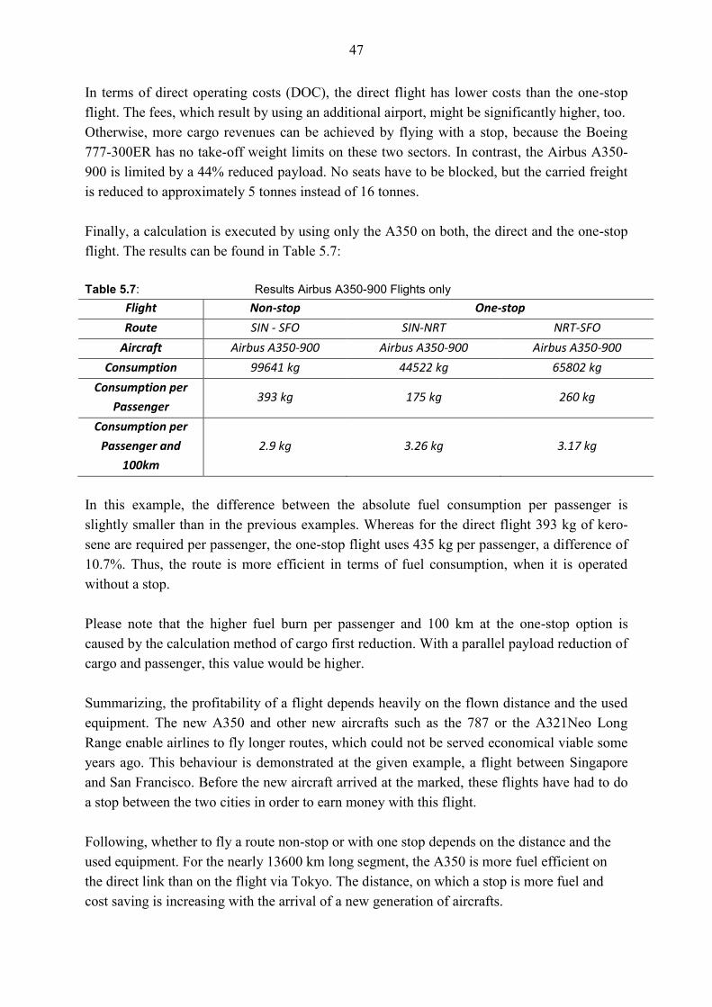
Finally, a calculation is executed by using only the A350 on both, the direct and the one-stop

flight. The results can be found in Table 5.7:

Table 5.7: Results Airbus A350-900 Flights only



Aircraft Airbus A350-900 Airbus A350-900 Airbus A350-900


Consumption per


Consumption per

Passenger and

100km

2.9 kg 3.26 kg 3.17 kg

In this example, the difference between the absolute fuel consumption per passenger is

slightly smaller than in the previous examples. Whereas for the direct flight 393 kg of kero-

sene are required per passenger, the one-stop flight uses 435 kg per passenger, a difference of

10.7%. Thus, the route is more efficient in terms of fuel consumption, when it is operated

without a stop.

Please note that the higher fuel burn per passenger and 100 km at the one-stop option is

caused by the calculation method of cargo first reduction. With a parallel payload reduction of

cargo and passenger, this value would be higher.

Summarizing, the profitability of a flight depends heavily on the flown distance and the used

equipment. The new A350 and other new aircrafts such as the 787 or the A321Neo Long

Range enable airlines to fly longer routes, which could not be served economical viable some

years ago. This behaviour is demonstrated at the given example, a flight between Singapore

and San Francisco. Before the new aircraft arrived at the marked, these flights have had to do

a stop between the two cities in order to earn money with this flight.

Following, whether to fly a route non-stop or with one stop depends on the distance and the

used equipment. For the nearly 13600 km long segment, the A350 is more fuel efficient on

the direct link than on the flight via Tokyo. The distance, on which a stop is more fuel and

cost saving is increasing with the arrival of a new generation of aircrafts.

48

Because of new aircrafts, more and more long-haul flights are accessed. The direct flight be-

tween Singapore and San Francisco was inaugurated after the arrival of the A350 at Singapore

Airlines (Singapore Air 2017).

5.3 Conclusion

With the fuel calculation based on the weights extracted from the payload range chart, a rough

insight into the fuel consumption in commercial aviation can be achieved. The numbers dem-

onstrate the development of the aircraft’s efficiency, especially on long range flights.

With modern aircrafts, a fuel reduction of 40% on the same route with nearly the same pas-

senger load is possible. This achievement is enabled through the use of lightweight materials

such as carbon fibre reinforced polymer and the increased technical reliability, which enables

the use of two engines instead of three or four.

Additionally, the air contamination and exhaust gas pollution is reduced by the saving of fuel.

The increasing distance of new developed routes is enabled through new developed aircrafts

such as Airbus A350 or Boeing 787. With this aircraft, long distance city pairs can be served

economically. The abandonment of a stop can save time, money and even fuel. But as long as

other airplanes than the previous mentioned are used on very long flights, the non-stop flight

might be fuel and economically inefficient, since a payload reduction, leading to blocked seats

and lower revenues, is necessary.

For the customer, one-stop flights are often cheaper, but require more time and a longer flight

distance than a non-stop flight. The calculation shows that a non-stop flight, e.g. Singapore to

San Francisco has a lower fuel consume than a one-stop flight, if the flight is operated by an

A350.

It has to be considered, that one-stop flights are mostly directed via hubs. As a consequence,

the passenger’s transfer stop is the final destination for the flight and not a stop between the

flights. There are less flights remaining which use a stop as a fuel stop to continue the flight

afterwards.

Airlines such as Iceland Air, Finnair or the gulf Airlines (Emirates Airlines, Qatar Airways

and Etihad Airways), which make heavily use of its geographical positioned hubs, will face

higher competition since other carriers e.g. Lufthansa or British Airways can fly with the

newly arrived aircraft longer sectors on profitable basis and can offer more competitive prices

to the costumer.

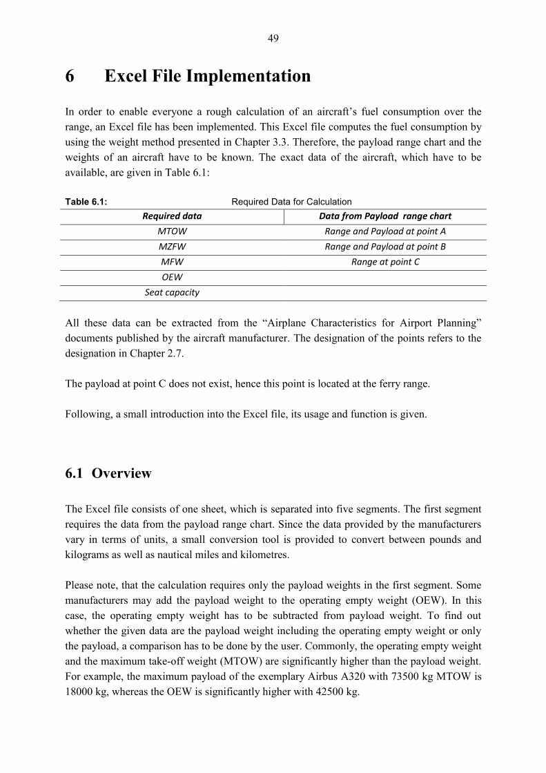
49

6 Excel File Implementation

In order to enable everyone a rough calculation of an aircraft’s fuel consumption over the

range, an Excel file has been implemented. This Excel file computes the fuel consumption by

using the weight method presented in Chapter 3.3. Therefore, the payload range chart and the

weights of an aircraft have to be known. The exact data of the aircraft, which have to be

available, are given in Table 6.1:

Table 6.1: Required Data for Calculation

Required data Data from Payload range chart

MTOW Range and Payload at point A

MZFW Range and Payload at point B

MFW Range at point C

OEW

Seat capacity

All these data can be extracted from the “Airplane Characteristics for Airport Planning”

documents published by the aircraft manufacturer. The designation of the points refers to the

designation in Chapter 2.7.

The payload at point C does not exist, hence this point is located at the ferry range.

Following, a small introduction into the Excel file, its usage and function is given.

6.1 Overview

The Excel file consists of one sheet, which is separated into five segments. The first segment

requires the data from the payload range chart. Since the data provided by the manufacturers

vary in terms of units, a small conversion tool is provided to convert between pounds and

kilograms as well as nautical miles and kilometres.

Please note, that the calculation requires only the payload weights in the first segment. Some

manufacturers may add the payload weight to the operating empty weight (OEW). In this

case, the operating empty weight has to be subtracted from payload weight. To find out

whether the given data are the payload weight including the operating empty weight or only

the payload, a comparison has to be done by the user. Commonly, the operating empty weight

and the maximum take-off weight (MTOW) are significantly higher than the payload weight.

For example, the maximum payload of the exemplary Airbus A320 with 73500 kg MTOW is

18000 kg, whereas the OEW is significantly higher with 42500 kg.

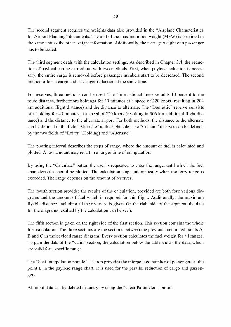
50

The second segment requires the weights data also provided in the “Airplane Characteristics

for Airport Planning” documents. The unit of the maximum fuel weight (MFW) is provided in

the same unit as the other weight information. Additionally, the average weight of a passenger

has to be stated.

The third segment deals with the calculation settings. As described in Chapter 3.4, the reduc-

tion of payload can be carried out with two methods. First, when payload reduction is neces-

sary, the entire cargo is removed before passenger numbers start to be decreased. The second

method offers a cargo and passenger reduction at the same time.

For reserves, three methods can be used. The “International” reserve adds 10 percent to the

route distance, furthermore holdings for 30 minutes at a speed of 220 knots (resulting in 204

km additional flight distance) and the distance to alternate. The “Domestic” reserve consists

of a holding for 45 minutes at a speed of 220 knots (resulting in 306 km additional flight dis-

tance) and the distance to the alternate airport. For both methods, the distance to the alternate

can be defined in the field “Alternate” at the right side. The “Custom” reserves can be defined

by the two fields of “Loiter” (Holding) and “Alternate”.

The plotting interval describes the steps of range, where the amount of fuel is calculated and

plotted. A low amount may result in a longer time of computation.

By using the “Calculate” button the user is requested to enter the range, until which the fuel

characteristics should be plotted. The calculation stops automatically when the ferry range is

exceeded. The range depends on the amount of reserves.

The fourth section provides the results of the calculation, provided are both four various dia-

grams and the amount of fuel which is required for this flight. Additionally, the maximum

flyable distance, including all the reserves, is given. On the right side of the segment, the data

for the diagrams resulted by the calculation can be seen.

The fifth section is given on the right side of the first section. This section contains the whole

fuel calculation. The three sections are the sections between the previous mentioned points A,

B and C in the payload range diagram. Every section calculates the fuel weight for all ranges.

To gain the data of the “valid” section, the calculation below the table shows the data, which

are valid for a specific range.

The “Seat Interpolation parallel” section provides the interpolated number of passengers at the

point B in the payload range chart. It is used for the parallel reduction of cargo and passen-

gers.

All input data can be deleted instantly by using the “Clear Parameters” button.

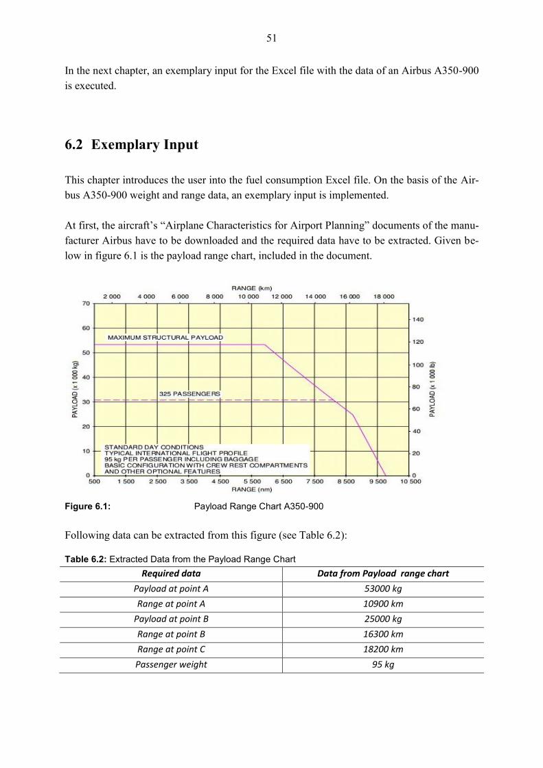
51

In the next chapter, an exemplary input for the Excel file with the data of an Airbus A350-900

is executed.

6.2 Exemplary Input

This chapter introduces the user into the fuel consumption Excel file. On the basis of the Air-

bus A350-900 weight and range data, an exemplary input is implemented.

At first, the aircraft’s “Airplane Characteristics for Airport Planning” documents of the manu-

facturer Airbus have to be downloaded and the required data have to be extracted. Given be-

low in figure 6.1 is the payload range chart, included in the document.

Figure 6.1: Payload Range Chart A350-900

Following data can be extracted from this figure (see Table 6.2):

Table 6.2: Extracted Data from the Payload Range Chart

Required data Data from Payload range chart

Payload at point A 53000 kg

Range at point A 10900 km

Payload at point B 25000 kg

Range at point B 16300 km

Range at point C 18200 km

Passenger weight 95 kg

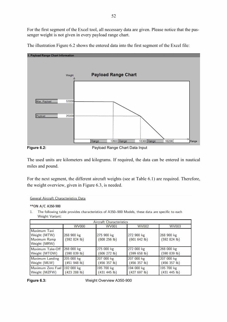
52

For the first segment of the Excel tool, all necessary data are given. Please notice that the pas-

senger weight is not given in every payload range chart.

The illustration Figure 6.2 shows the entered data into the first segment of the Excel file:

Figure 6.2: Payload Range Chart Data Input

The used units are kilometers and kilograms. If required, the data can be entered in nautical

miles and pound.

For the next segment, the different aircraft weights (see at Table 6.1) are required. Therefore,

the weight overview, given in Figure 6.3, is needed.

Figure 6.3: Weight Overview A350-900

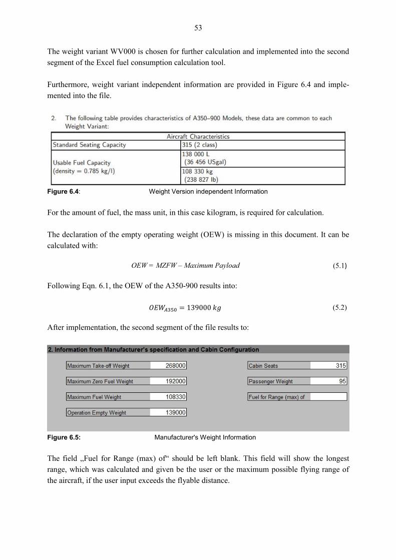
53

The weight variant WV000 is chosen for further calculation and implemented into the second

segment of the Excel fuel consumption calculation tool.

Furthermore, weight variant independent information are provided in Figure 6.4 and imple-

mented into the file.

Figure 6.4: Weight Version independent Information

For the amount of fuel, the mass unit, in this case kilogram, is required for calculation.

The declaration of the empty operating weight (OEW) is missing in this document. It can be

calculated with:

OEW = MZFW – Maximum Payload (5.1)

Following Eqn. 6.1, the OEW of the A350-900 results into:

(5.2)

After implementation, the second segment of the file results to:

Figure 6.5: Manufacturer's Weight Information

The field „Fuel for Range (max) of“ should be left blank. This field will show the longest

range, which was calculated and given be the user or the maximum possible flying range of

the aircraft, if the user input exceeds the flyable distance.

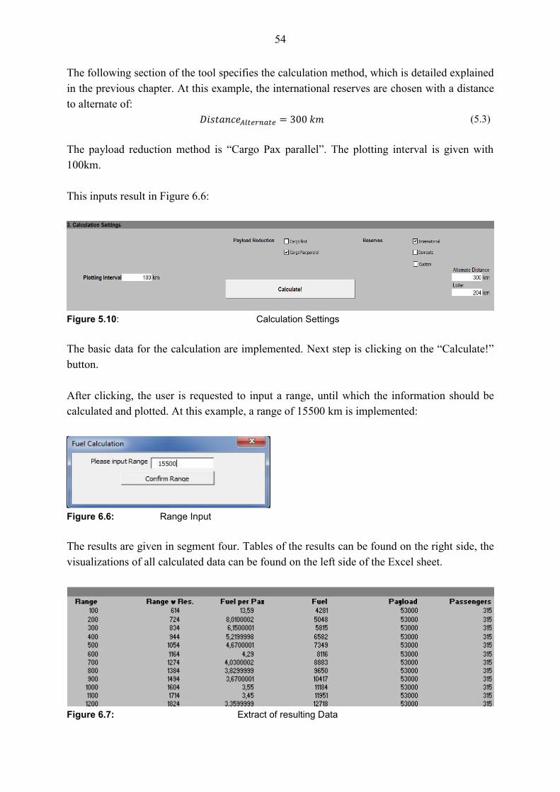
54

The following section of the tool specifies the calculation method, which is detailed explained

in the previous chapter. At this example, the international reserves are chosen with a distance

to alternate of:

(5.3)

The payload reduction method is “Cargo Pax parallel”. The plotting interval is given with

100km.

This inputs result in Figure 6.6:

Figure 5.10: Calculation Settings

The basic data for the calculation are implemented. Next step is clicking on the “Calculate!”

button.

After clicking, the user is requested to input a range, until which the information should be

calculated and plotted. At this example, a range of 15500 km is implemented:

Figure 6.6: Range Input

The results are given in segment four. Tables of the results can be found on the right side, the

visualizations of all calculated data can be found on the left side of the Excel sheet.

Figure 6.7: Extract of resulting Data

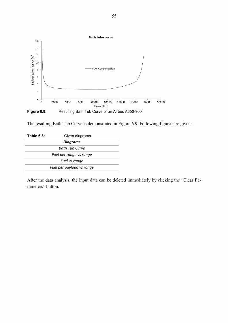
55

Figure 6.8: Resulting Bath Tub Curve of an Airbus A350-900

The resulting Bath Tub Curve is demonstrated in Figure 6.9. Following figures are given:

Table 6.3: Given diagrams

Diagrams

Bath Tub Curve

Fuel per range vs range

Fuel vs range

Fuel per payload vs range

After the data analysis, the input data can be deleted immediately by clicking the “Clear Pa-

rameters” button.

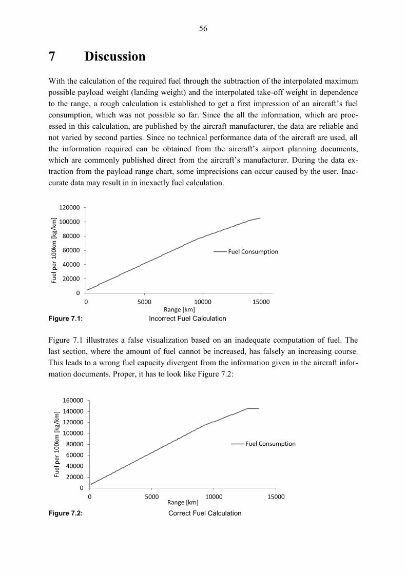
56

7 Discussion

With the calculation of the required fuel through the subtraction of the interpolated maximum

possible payload weight (landing weight) and the interpolated take-off weight in dependence

to the range, a rough calculation is established to get a first impression of an aircraft’s fuel

consumption, which was not possible so far. Since the all the information, which are proc-

essed in this calculation, are published by the aircraft manufacturer, the data are reliable and

not varied by second parties. Since no technical performance data of the aircraft are used, all

the information required can be obtained from the aircraft’s airport planning documents,

which are commonly published direct from the aircraft’s manufacturer. During the data ex-

traction from the payload range chart, some imprecisions can occur caused by the user. Inac-

curate data may result in in inexactly fuel calculation.

Figure 7.1: Incorrect Fuel Calculation

Figure 7.1 illustrates a false visualization based on an inadequate computation of fuel. The

last section, where the amount of fuel cannot be increased, has falsely an increasing course.

This leads to a wrong fuel capacity divergent from the information given in the aircraft infor-

mation documents. Proper, it has to look like Figure 7.2:

Figure 7.2: Correct Fuel Calculation

0

20000

40000

60000

80000

100000

120000

0 5000 10000 15000

Fuel

per

10

0km

[kg

/km

]

Range [km]

Fuel Consumption

0

20000

40000

60000

80000

100000

120000

140000

160000

0 5000 10000 15000

Fuel

per

10

0km

[kg

/km

]

Range [km]

Fuel Consumption

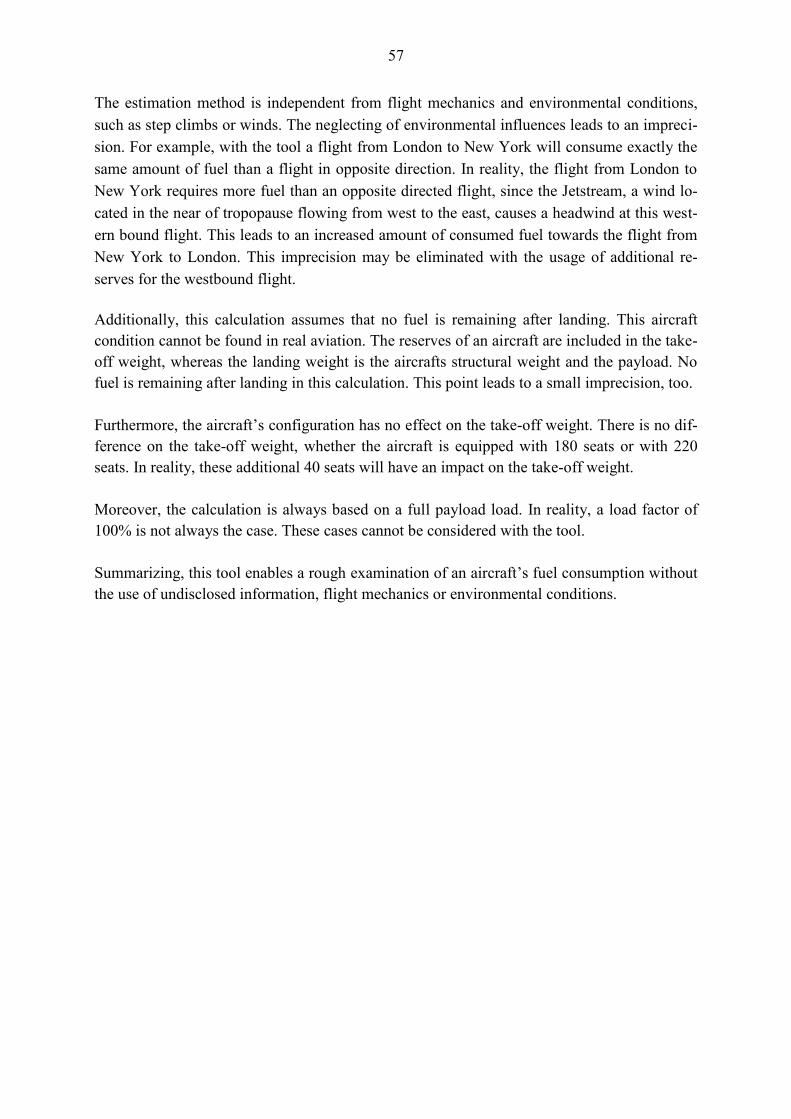
57

The estimation method is independent from flight mechanics and environmental conditions,

such as step climbs or winds. The neglecting of environmental influences leads to an impreci-

sion. For example, with the tool a flight from London to New York will consume exactly the

same amount of fuel than a flight in opposite direction. In reality, the flight from London to

New York requires more fuel than an opposite directed flight, since the Jetstream, a wind lo-

cated in the near of tropopause flowing from west to the east, causes a headwind at this west-

ern bound flight. This leads to an increased amount of consumed fuel towards the flight from

New York to London. This imprecision may be eliminated with the usage of additional re-

serves for the westbound flight.

Additionally, this calculation assumes that no fuel is remaining after landing. This aircraft

condition cannot be found in real aviation. The reserves of an aircraft are included in the take-

off weight, whereas the landing weight is the aircrafts structural weight and the payload. No

fuel is remaining after landing in this calculation. This point leads to a small imprecision, too.

Furthermore, the aircraft’s configuration has no effect on the take-off weight. There is no dif-

ference on the take-off weight, whether the aircraft is equipped with 180 seats or with 220

seats. In reality, these additional 40 seats will have an impact on the take-off weight.

Moreover, the calculation is always based on a full payload load. In reality, a load factor of

100% is not always the case. These cases cannot be considered with the tool.

Summarizing, this tool enables a rough examination of an aircraft’s fuel consumption without

the use of undisclosed information, flight mechanics or environmental conditions.

58

8 Summary

In this project, the possibility of fuel calculation based on aircraft manufacturer information

was investigated, regarding to the project of Wullbrand and the master thesis of MacDonald.

The required information is the payload range chart and some weight information. Both can

be extracted from the airport planning documents of an aircraft.

The “Bath Tub Curve” was established with the results of the flight mechanics calculation.

The calculation itself was refined in two ways: First, the Breguet Factor, which has been

computed at three points, was now calculated in smaller intervals in order to achieve a more

detailed calculation. Furthermore, the Fuel Fraction was eliminated, hence the adjusted

Breguet Factor yields accurate results without the use of the Fuel Fraction.

The accuracy of the generated data was proved by the interpolation of the take-off and landing

weights. Since this data correspond exactly with the results of the calculation, a computation

only based on the subtraction of take-off and landing weights was introduced. The flight me-

chanics can be neglected on this way of calculation, which enables the user a plain calculation

of an aircraft’s fuel consumption.

On the basis of the computed fuel calculation, various fuel visualizations can be plotted. For

example, the aircraft efficiency depending on the flight length can be illustrated with the Bath

Tub Curve, where the fuel consumption per passenger and 100 km flight distance over the

range are demonstrated. Moreover, other visualizations were investigated and discussed. The

coherence of all this charts has been found out. Resulting, the fuel per range chart affects the

Bath Tub Curve at smaller ranges, whereas the fuel per payload chart affects the Bath Tub

Curve at greater distances the most.

The information gained from the fuel calculation was following related to aircraft operation

today. The flight sector between Hong Kong and Frankfurt was analysed with regard to air-

crafts of different decades. Resulting, the Boeing 747-200B, which was used until the 1990s

on this sector needs around 40% more fuel than a new generation Airbus A350-1000 to carry

roughly the same amount of passengers on this sector.

It was also investigated, whether to fly a sector non-stop or with a stop in between. The ana-

lysed city pair was Singapore and San Francisco with an optional stop in Tokyo. Every com-

bination with an Airbus A350-900 and a Boeing 777-300ER used on these sectors were com-

pared. Resulting, a direct flight of an A350-900 is the most fuel efficient option. As long as

the range can be flown in an efficient area of the Bath Tub Curve, a stop between is the more

fuel consuming option. Nevertheless, the geographical position and the hub and spoke system

of an airline, which offers a one-stop option, have to be considered.

59

Following, the established Excel file was explained and an exemplary input was made to ease

the usage of this tool, including the extraction of the weight and range information as well as

the adjustment of the reserves.

Finally, the discussion highlighted the inaccuracies of the calculation method. Exemplary, the

environmental conditions or flight mechanics are not considered directly within the calcula-

tion. They can be adjusted within the reserves. Summarizing, the fuel calculation offers a

roughly estimation based on the aircraft manufacturer’s information.

Referring to the information stated by Lufthansa, where the overall fleet fuel consumption in

2016 is given with 3.85 litres (which corresponds 3.08kg fuel) per passenger and 100 km

flight distance (Lufthansa 2017), it can be assumed that this amount may be accurate follow-

ing the results of this project.

60

References

Airbus 2016 AIRBUS - TECHNICAL DATA SUPPORT AND SERVICES: A350 Aircraft

Characteristics Airport and Maintenance Planning. Toulouse, 2016. –

URL:

http://www.aircraft.airbus.com/fileadmin/media_gallery/files/tech_dat

a/AC/Airbus_AC_A350XWB-Jun16.pdf (15.10.2017)

Boeing 2011 BOEING COMMERCIAL AIRRCRAFT COMPANY: Boeing 747 Airplane

Characteristics – Airport Planning. Seattle, 2011. – URL:

http://www.boeing.com/resources/boeingdotcom/commercial/airports/

acaps/747_123sp.pdf (03.11.2017)

Boeing 2015 BOEING COMMERCIAL AIRRCRAF COMPANY: Boeing 777-200LR/ -

300ER/ -Freighter Airplane Characteristics for Airport Planning. Se-

attle, 2015. – URL:

http://www.boeing.com/resources/boeingdotcom/commercial/airports/

acaps/777_2lr3er.pdf (03.11.2017)

Cathay 2017 URL: https://www.cathaypacific.com/cx/de_DE/travel-

information/flying-with-us/aircraft-and-fleet/boeing-777/300.html

(06.11.2017)

Flightaware 2017 URL: https://de.flightaware.com (05.11.2017)

Frequent 2012 URL:http://frequentlyflying.boardingarea.com/vintage-airline-seat-

map-cathay-pacific-boeing-747-200-1980s (06.11.2017)

Lufthansa 2017 WALTHER, Claudia; MILCHSACK, Steffen: Balance : Key data of sus-

tainability within the Lufthansa Group. Cologne, 2017. - URL:

https://www.lufthansagroup.com/fileadmin/downloads/en/responsibilit

y/balance-2017-epaper/#40 (20.09.2017)

MacDonald 2012 MACDONALD, ALLEN: A General view on Fuel Efficiency in Commer-

cial Aviation. Hamburg, HAW Hamburg, Department of Automotive

Engineering, Master Thesis, 2012

http://www.aircraft.airbus.com/fileadmin/media_gallery/files/tech_data/AC/Airbus_AC_A350XWB-Jun16.pdf

http://www.aircraft.airbus.com/fileadmin/media_gallery/files/tech_data/AC/Airbus_AC_A350XWB-Jun16.pdf

http://www.boeing.com/resources/boeingdotcom/commercial/airports/acaps/747_123sp.pdf

http://www.boeing.com/resources/boeingdotcom/commercial/airports/acaps/747_123sp.pdf

http://www.boeing.com/resources/boeingdotcom/commercial/airports/acaps/777_2lr3er.pdf

http://www.boeing.com/resources/boeingdotcom/commercial/airports/acaps/777_2lr3er.pdf

https://www.cathaypacific.com/cx/de_DE/travel-information/flying-with-us/aircraft-and-fleet/boeing-777/300.html

https://www.cathaypacific.com/cx/de_DE/travel-information/flying-with-us/aircraft-and-fleet/boeing-777/300.html

https://de.flightaware.com/

http://frequentlyflying.boardingarea.com/vintage-airline-seat-map-cathay-pacific-boeing-747-200-1980s/

http://frequentlyflying.boardingarea.com/vintage-airline-seat-map-cathay-pacific-boeing-747-200-1980s/

https://www.lufthansagroup.com/fileadmin/downloads/en/responsibility/balance-2017-epaper/%2340

https://www.lufthansagroup.com/fileadmin/downloads/en/responsibility/balance-2017-epaper/%2340

61

NACA 1969 NATIONAL ADVISORY COMMITTEE FOR AERONAUTICS: A Study of Air-

plane Ranges and useful Loads. Washington D.C.: NACA, 1969 (Re-

port Nr. 69) URL:

http://naca.central.cranfield.ac.uk/reports/1920/naca-report-

69.pdf(28.11.2017)

Scholz 2016 SCHOLZ, DIETER: Flugmechanik. Hamburg, HAW Hamburg, Depart-

ment of Automotive Engineering, Lecture 2013

Singapore Air 2017 URL:http://www.singaporeair.com/de_DE/de/flying-withus/our-

story/our-fleet (06.11.2017)

Wulbrand 2016 WULBRAND, FINN: Treibstoffverbrauch bei extrem kurzen und extrem

langen Flügen. HAW Hamburg, Department of Automotive Engineer-

ing, Project, 2016

http://naca.central.cranfield.ac.uk/reports/1920/naca-report-69.pdf

http://naca.central.cranfield.ac.uk/reports/1920/naca-report-69.pdf

http://www.singaporeair.com/de_DE/de/flying-withus/our-story/our-fleet/airbus-a350-900/

http://www.singaporeair.com/de_DE/de/flying-withus/our-story/our-fleet/airbus-a350-900/

Documents

Aircraft Fuel Consumption – Estimation and …...DEPARTMENT OF AUTOMOTIVE AND AERONAUTICAL ENGINEERING Aircraft Fuel Consumption – Estimation and Visualization Task for a Project