AIX MARSEILLE UNIVERSITE ECOLE CENTRALE DE …doc.centrale-marseille.fr/TFE/inter2016/Bounissou_Sophie_Rapport.pdf · HSIM HARMONI Simulator i inclination IFS Integral Field Spectroscopy

AIX MARSEILLE UNIVERSITE

ECOLE CENTRALE DE MARSEILLE

LABORATOIRE D'ASTROPHYSIQUE DE

MARSEILLE

UNIVERSITY OF OXFORD

SOPHIE BOUNISSOU

SIMULATIONS FOR THE HARMONI

INTEGRAL FIELD SPECTROGRAPH

FOR THE EUROPEAN ELT

MSc THESIS

AIX MARSEILLE UNIVERSITEECOLE CENTRALE DE MARSEILLE

LABORATOIRE D'ASTROPHYSIQUE DE MARSEILLEUNIVERSITY OF OXFORD

MSc THESIS

Academic Year 2015-16

SOPHIE BOUNISSOU

Simulations for the HARMONI integral eld spectrograph

on the European ELT

Supervisors:

Jean-Yves Natoli (AMU)

Frédéric Lemarquis (ECM)

Benoit Neichel (LAM)

Niranjan Thatte (UOx)

April - August 2016

i

Abstract

This master thesis is the result of the ve month's work within the HARMONIconsortium. HARMONI will be the rst-light spectroscopic capability of the 39-m European Extremely Large Telescope (E-ELT). At the present time the designphase is still ongoing and instrument simulations are vital to understanding the ca-pabilities and limitations of the instrument design in achieving certain science goals.With this purpose in mind, the University of Oxford has developed the HARMONISIMulator (HSIM), a simulation pipeline to mimic as realistically as possible the ob-servations with E-ELT and especially with HARMONI. This report describes brieythe E-ELT project and the HARMONI integral eld spectrograph. We then focus onHSIM simulation methodology, which has been a key component during this study.Two studies are presented: the supernovae project and the Hα kinematics survey ofgalaxies.

For the supernovae project, we simulate supernovae type Ia into a galaxy at highredshift and we try to detect them after running HSIM. For this purpose, we performa signal-to-noise study in order to optimize the aperture size from which the super-nova is extracted. Then a method using cross-correlation is implemented in orderto recover the physical information of supernovae at dierent luminosities. Finally,we use on the same spectra templates the Supert program, which is a more robusttting code. This last step, as well as providing another analysis tool, allows tomake suggestions for possible improvements on the cross-correlation method. Thesupernova project conrms that observations of SN Ia at high redshift withe E-ELTwill be possible even for many days after maximum-light.

Concerning the Hα kinematics survey, galaxies observed in the local Universe areredshifted to a higher z and we then simulate observations with HARMONI. Study-ing kinematics of a galaxy means studying the relative velocity of matter inside thegalaxy. In this study, this is achieved by observing the shift of the Hα wavelength(656.3 nm). Velocity eld maps for 45 galaxies are derived from the Hα observationusing the Doppler-Fizeau eect. From velocity eld maps, we can plot the rotationcurves of galaxies and in this way compare data of the local Universe from dataobserved with HARMONI at higher redshift.

With these two studies, this thesis only shows a small part of the possibilities withthe HARMONI integral eld spectrograph.

ii

iii

Acknowledgements

There are many people I want to thank for helping me to achieve this thesis in thebest conditions:

• Benoit Epinat, researcher in the HARMONI team, for his presence and hispatience (especially when he explained me some physics of galaxies!), I learnta lot of little tricks in coding thanks to him;

• Benoit Neichel, researcher in the HARMONI team, for giving me the op-portunity to do my master thesis inside the HARMONI consortium and foranswering to all my questions about HARMONI and adaptive optics;

• Niranjan Thatte, the HARMONI Principal Investigator, for his kindness, hisactive encouragements and for all the time he spends with me despite he wasso busy. I was lucky to learn from him and I hope I could work with himagain;

• Simon Zieleniewski, Postdoc in the HARMONI team, and because I know howmuch he loves to speak this language, I switch to French !Donc je tenais à remercier vivement Simon, sans qui ce stage n'aurait jamaiseu lieu, tout simplement parce que son simulateur est au coeur de mon travail.Cela a toujours été enrichissant, et souvent très amusant, de travailler à sescôtés. Merci également pour la relecture méticuleuse du projet SN;

• the HARMONI team, especially Vanessa Ferraro-Wood, the HARMONI ProjectAdministrator, who takes good care of me when I rst arrived in Oxford andRyan Houghton, researcher in the HARMONI team, who gives me great ad-vices for spectra analysis;

• the Marseille LOOM team, who I have now known for a long time, and partic-ularly Emmanuel Hugot, the Head of LAM R&D group. I owe him everything!

iv

CONTENTS v

Contents

Contents v

List of gures vii

List of tables ix

Abbreviations x

1 Introduction 1

1.1 The European Extremely Large Telescope . . . . . . . . . . . . . . . 1

1.1.1 Astronomy with E-ELT . . . . . . . . . . . . . . . . . . . . . 1

1.1.2 Technological advances with the biggest telescope ever built . 2

1.2 The HARMONI Integral Field Spectrograph . . . . . . . . . . . . . . 3

1.2.1 Integral Field Spectroscopy . . . . . . . . . . . . . . . . . . . 3

1.2.2 HARMONI . . . . . . . . . . . . . . . . . . . . . . . . . . . . 5

1.3 The simulation pipeline HSIM . . . . . . . . . . . . . . . . . . . . . . 7

1.3.1 Simulation methodology . . . . . . . . . . . . . . . . . . . . . 7

1.3.2 HSIM interface . . . . . . . . . . . . . . . . . . . . . . . . . . 8

1.4 Project overview . . . . . . . . . . . . . . . . . . . . . . . . . . . . . 9

2 Supernovae project 11

2.1 Supernovae physics . . . . . . . . . . . . . . . . . . . . . . . . . . . . 11

2.1.1 Supernovae classication . . . . . . . . . . . . . . . . . . . . . 11

vi Contents

2.1.2 SNe Ia as standard candles . . . . . . . . . . . . . . . . . . . . 13

2.2 SN-Ia simulations inside a galaxy . . . . . . . . . . . . . . . . . . . . 16

2.2.1 Magnitude calculations for the host galaxy . . . . . . . . . . . 16

2.2.2 SNe magnitude calibrations . . . . . . . . . . . . . . . . . . . 19

2.3 Simulating SN-Ia observations through HSIM . . . . . . . . . . . . . 21

2.3.1 Running HSIM . . . . . . . . . . . . . . . . . . . . . . . . . . 22

2.3.2 Optimizing the Signal-to-Noise Ratio . . . . . . . . . . . . . . 23

2.4 Supernovae classication . . . . . . . . . . . . . . . . . . . . . . . . . 26

2.4.1 Cross-Correlation method . . . . . . . . . . . . . . . . . . . . 26

2.4.2 Minimum χ2 method and conclusions . . . . . . . . . . . . . . 28

3 Hα kinematic survey of galaxies 31

3.1 Hα kinematics and input data . . . . . . . . . . . . . . . . . . . . . . 31

3.1.1 Hα kinematics . . . . . . . . . . . . . . . . . . . . . . . . . . . 31

3.1.2 Input data cubes for HSIM . . . . . . . . . . . . . . . . . . . . 32

3.2 Observing galaxies with HSIM and data processing with Camel . . . 33

3.2.1 Running HSIM . . . . . . . . . . . . . . . . . . . . . . . . . . 34

3.2.2 Running Camel for 2D velocity eld maps . . . . . . . . . . . 36

3.2.3 Rotation curves . . . . . . . . . . . . . . . . . . . . . . . . . . 37

4 Conclusion 39

References 39

A Appendix of the SN project 42

B Appendix of the Hα kinematics survey 45

LIST OF FIGURES vii

List of Figures

1.1 European Extremely Large Telescope . . . . . . . . . . . . . . . . . . 3

1.2 Principle of spectrography . . . . . . . . . . . . . . . . . . . . . . . . 4

1.3 Integral Field Spectroscopy principle with image slicer . . . . . . . . 5

1.4 Spaxel scales and corresponding FoV for HARMONI . . . . . . . . . 6

1.5 Flowchart of the HSIM simulation process . . . . . . . . . . . . . . . 7

1.6 HSIM graphical user interface . . . . . . . . . . . . . . . . . . . . . . 8

2.1 Crab Nebula or M1: a supernova remnant . . . . . . . . . . . . . . . 12

2.2 Schematic light curves for SNe of Types Ia, Ib, II-L, II-P, and SN 1987A 13

2.3 Spectra of SNe Ia about one week past maximum brightness . . . . . 14

2.4 Light curves of nearby, low-redshift type Ia supernovae measured byMario Hamuy and coworkers. . . . . . . . . . . . . . . . . . . . . . . 15

2.5 View of a section of the galaxy data cube . . . . . . . . . . . . . . . . 17

2.6 Integrated stellar spectra of the z=3 RAMSES galaxy . . . . . . . . . 18

2.7 Integrated stellar spectra of the galaxy in rest-frame . . . . . . . . . . 19

2.8 Spectra of types Ia, Ib/c, Ic and II over the B-V range . . . . . . . . 21

2.9 Spectrum of a type Ia (SN1981b) supernova at maximum light . . . . 22

2.10 View of the observed data cube with supernova within the host galaxy 24

2.11 Signal-to-Noise Ratio versus the linear size of square box at maximumlight . . . . . . . . . . . . . . . . . . . . . . . . . . . . . . . . . . . . 25

2.12 Signal-to-Noise Ratio versus wavelength at maximum light . . . . . . 26

2.13 Extracted spectrum and associated background variance at maximumlight with a rebinning of 9 pixels . . . . . . . . . . . . . . . . . . . . . 28

viii LIST OF FIGURES

2.14 List of the Supert best matches for the SNIa at r=2.4% . . . . . . . 30

3.1 Galaxy UGC 7045 before running HSIM . . . . . . . . . . . . . . . . 34

3.2 Galaxy UGC 7045 after running HSIM (20×20 mas scale) . . . . . . 35

3.3 Galaxy UGC 7045 after running HSIM (30×60 mas scale) . . . . . . 36

3.4 Velocity eld maps of the galaxy UGC 7045 for two spaxel scales . . . 37

3.5 Rotation curves of the galaxy UGC 7045 . . . . . . . . . . . . . . . . 38

A.1 View of the observed data cube with supernova within the host galaxy 42

A.2 Signal-to-Noise Ratio versus wavelength at dierent stages . . . . . . 43

A.3 Extracted spectrum and associated background variance for dierentluminosity . . . . . . . . . . . . . . . . . . . . . . . . . . . . . . . . . 44

LIST OF TABLES ix

List of Tables

1.1 FITS le header keys required for input data cubes in HSIM . . . . . 9

2.1 Cosmological parameters for deriving the luminosity distance . . . . . 17

2.2 Photometric zero points (Vega system) . . . . . . . . . . . . . . . . . 20

2.3 Absolute-magnitude distribution of seven supernova types . . . . . . 20

2.4 Ratio between luminosity of the SN and luminosity of the galaxy . . . 20

2.5 HARMONI simulator input parameters . . . . . . . . . . . . . . . . . 23

2.6 Binning and resulting averaged SNR for dierent SN luminosity . . . 27

2.7 Cross-correlation factor between observed Ia and other spectra atdierent stages . . . . . . . . . . . . . . . . . . . . . . . . . . . . . . 29

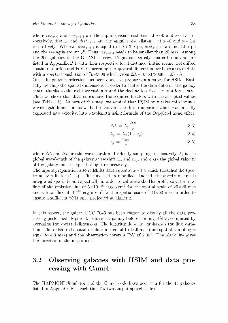
3.1 HARMONI simulator input parameters . . . . . . . . . . . . . . . . . 35

B.1 List of galaxies used for simulations with their distance, the initialobserving seeing, the redshifted spatial resolution and the FoV . . . . 46

x Abbreviations

Abbreviations

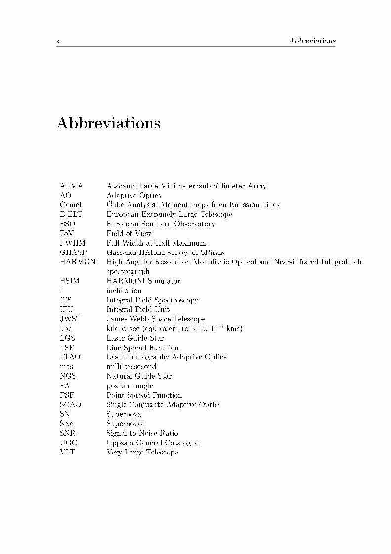
ALMA Atacama Large Millimeter/submillimeter ArrayAO Adaptive OpticsCamel Cube Analysis: Moment maps from Emission LinesE-ELT European Extremely Large TelescopeESO European Southern ObservatoryFoV Field-of-ViewFWHM Full Width at Half MaximumGHASP Gassendi HAlpha survey of SPiralsHARMONI High Angular Resolution Monolithic Optical and Near-infrared Integral eld

spectrographHSIM HARMONI Simulatori inclinationIFS Integral Field SpectroscopyIFU Integral Field UnitJWST James Webb Space Telescopekpc kiloparsec (equivalent to 3.1 x 1016 kms)LGS Laser Guide StarLSF Line Spread FunctionLTAO Laser Tomography Adaptive Opticsmas milli-arcsecondNGS Natural Guide StarPA position anglePSF Point Spread FunctionSCAO Single Conjugate Adaptive OpticsSN SupernovaSNe SupernovaeSNR Signal-to-Noise RatioUGC Uppsala General CatalogueVLT Very Large Telescope

Introduction 1

Chapter 1

Introduction

This thesis study into the simulations of scientic observations using the HARMONIinstrument was proposed by the international HARMONI consortium.

This chapter introduces the motivation for simulations with the HARMONI integraleld spectrograph and species the objectives and the scope of this research.

1.1 The European Extremely Large Telescope

1.1.1 Astronomy with E-ELT

Astronomy as a dynamic science has always pushed technological boundaries to gofurther in our knowledge of the Universe. Current ground- and spaced- telescopeprovide astronomers with unprecedented image quality and allow them to observefurther than ever before. However, humanity's insatiable quest to gain a deeper un-derstanding of the Universe means observational technology is always being furtherdeveloped.

In this context, the European Southern Observatory (ESO) leads the design, con-struction and operation of ground-based telescopes in the southern hemisphere. TheAtacama desert in Chile seems to be its preferred terrain for astronomical facilitieswith exceptional seeing conditions due to altitude and dryness. In 2014, the 39-meterEuropean Extremely Large Telescope (E-ELT) project was ocially launched andits rst light is planned a decade later on the top of the Cerro Armazones (3060 m),20 kilometers from the Cerro Paranal, home of the Very Large Telescope (VLT). TheE-ELT will be the world's largest ground-based optical telescope and will work in astrong synergy with the Atacama Large Millimeter/sub-millimeter Array (ALMA,rst-light in 2011) and the James Webb Space Telescope (JWST, launch in 2018)to provide unprecedented observational insights as we enter the ÈLT' era.

2 Introduction

Using the E-ELT, ESO hopes to tackle many questions left open up until now. Forinstance, astronomers would like to probe other solar systems with rocky planetsin the "habitable zone" to try and determine the presence of liquid water on thesurface. The E-ELT should have the angular resolution and the sensitivity to imagedirectly these Earth-like-planets and to help analyze their atmospheric composition.Another challenge would be to complete the cosmological model that we have todate because only 5% of the cosmos is made of the known "normal matter", therest belongs to the mysterious "dark matter" and "dark energy". Observations withthe E-ELT should give some clues to astronomers to more accurately compute theaccelerating expansion of the Universe and to probe galaxies from their formationepoch. High resolution investigations of black holes will also hopefully reveal excit-ing new astrophysics.

The eld of possibilities in astronomy with the E-ELT seems to be innite andtherefore the associated technological requirements will be as challenging as thescientic objectives.

1.1.2 Technological advances with the biggest telescope ever

built

Nowadays with its two 10-meter telescopes, Keck Observatory in Hawaii standsamong the largest telescopes for visible and near-infrared observations. After havingabandoned the 100-meter Overwhelmingly Large (OWL) Telescope project whichwas considered unfeasible, ESO has kept pursuing the `biggest telescope' ethos bylaunching the E-ELT project with its unprecedented size.

What the astronomers call the "world's biggest eye on the sky" will have a 39-meterprimary mirror and thus will be able to collect 15 times more light than the currentoperating telescopes (Figure 1.1). It will revolutionize optical and near-infrared as-tronomy with the discoveries that will be made and also with the technological andengineering advances.

The E-ELT is based upon a ve-mirror design. To reach a 39-meter size, the primarymirror will be composed of almost 800 hexagonal mirrors, each 1.4 meters wide and5 cm thick, and will be supported by 6000 actuators. Then two other mirrors willrelay light through to the fourth and fth mirrors, which are part of an adaptiveoptics (AO) system and will adjust their shape in order to correct distortion fromthe turbulence of the Earth's atmosphere every millisecond. The AO system willwork with 6 laser guide stars (LGS), in addition to natural guide stars (NGS). Guidestars are observed close to the target under study and are used as a reference toprobe the atmospheric distortions and estimate the blurring caused by the atmo-sphere. In cases where no natural guide star is available (only 1% of the sky canbe observed with NGS) close to the object, articial stars are produced with a LGSsystem whose lasers shine in the sky and excite the sodium layer in the atmosphere,

Introduction 3

Figure 1.1: European Extremely Large Telescope will be the largest optical telescopeever built with its 39-meter primary mirror and 85-meter-diameter rotating dome.Credit ESO.

probing the turbulence prole. The use of AO is able to substantially improve imagequality, spatial resolution and sensitivity.

The E-ELT mirrors will relay light to dierent scientic instruments and will beable to switch from one instrument to another within minutes. These "rst-light"instruments are:

• HARMONI, High Angular Resolution Monolithic Optical and Near-infraredIntegral eld spectrograph

• MAORY, Multi-conjugate Adaptive Optics RelaY for the E-ELT

• METIS, Mid-infrared E-ELT Imager and Spectrograph

• MICADO, Multi-AO Imaging Camera for Deep Observations

1.2 The HARMONI Integral Field Spectrograph

1.2.1 Integral Field Spectroscopy

In astronomy and in many other elds, spectroscopy is a very powerful tool foranalysing light and thus characterising objects. Since Newton split white light intoa spectacular rainbow, astronomers have learnt how to read the spectra of distantstars. When a star produces a continuous spectrum, light travels and can pass

4 Introduction

through the gas of a nebula: some wavelengths can be absorbed by the molecules ofthis gas, this absorption leads to dark lines in the spectrum. On the contrary, whena photon is absorbed by an element of the gas, the absorbed energy is released byemitting another photon at a dierent wavelength, this corresponds to a bright linein the spectrum (Figure 1.2). Thanks to modern, electronic detectors like CCDs,astronomers can record spectra of stars and are then able to identify chemical ele-ments that caused absorption and emission lines. This data processing allows themto characterize the physics of astronomical objects.

Figure 1.2: Principle of spectrography: on a spectrum bright lines and dark linesare generated by the emission and absorption of photons respectively. Credit ESO.

Integral eld spectroscopy (IFS), contrary to long-split spectroscopy from whichyou get a one-dimensional spectrum (because one elongated slit aperture), collectsspectra of a whole eld of view (FoV). One substantial advantage compared tolong-slit spectroscopy is that IFS is a "point-and-shoot" capability, this means thatastronomers can point at the target object without extremely meticulous caution.An IFS can be achieved in three ways: using a lenslet array, optical bers or animage-slicer. In their concern to maximize throughput, IFS with image-slicers arepreferred by recent telescope facilities. Figure 1.3 shows the principle of IFS withthis technique. The sky-image is sliced and passes through the spectrograph, thencomputers can reconstruct the sky-image by rearrangering the slices according tothe input geometric pattern. The result of an IFS observation is a data cube (x, y,λ) with two spatial dimensions (x, y) and one spectral dimension (λ): a 2D-arrayof the FoV at dierent wavelengths. This data cube can been seen also as spectrafor each individual pixel.

Nearly all current and future telescopes have, or will have, spectrographs. In the

Introduction 5

Figure 1.3: Integra Field Spectroscopy principle with image slicer. Credit ESO.

context of getting the best from the available light gathering power of the telescope,HARMONI will function as the E-ELT's workhorse instrument for spectroscopy inthe visible and near-infrared wavelength range.

1.2.2 HARMONI

In September 2015, ESO signed an agreement with an international consortium ledby University of Oxford to build the HARMONI spectrograph at Oxford University.The HARMONI (High Angular Resolution Monolithic Optical and Near-infraredIntegral eld spectrograph) will be the rst light spectroscopic capability of theE-ELT, expected in 2024 (Thatte et al. 2014 [9]). The E-ELT's IFS will have awavelength coverage from 0.47 to 2.45 µm.

HARMONI will be able to take full advantage of the E-ELT's potential - especiallyits huge collecting area - and deal with its scientic goals thanks to a large rangeof spatial scale and resolving power options. Concerning the spatial resolution, theterm `spaxel' is used to describe a spatial pixel from the Integral Field Unit (IFU)and is expressed in milli-arcsecond (mas). A spaxel should be dierentiated from apixel of the detector. For HARMONI spaxel scales, four congurations have been

6 Introduction

chosen: 4×4 mas, 10×10 mas, 20×20 mas and 30×60 mas; an optical set-up allowsthe user to switch from one to each others. Figure 1.4 displays the FoV covered bythese ∼32000 spaxels according to their scale. Regarding the resolving powers, R isdened as equal to λ/∆λ and can take the values 3500, 7500 and 20000. The higherR, the smaller the spectral resolution ∆λ and the ner the spectra details that canbe detected.

Figure 1.4: Spaxel scales and corresponding FoV for HARMONI. The FoV has a√2:1 ratio at all scales. Note that the coarsest spaxel scale has rectangular spaxels

and its FoV is rotated by 90 degrees relative to the others. Credit (Thatte et al.2014 [9])

HARMONI will also be compatible with any adaptive optics mode: Laser Tomog-raphy Adaptive Optics (LTAO - high-level correction using LGS over most of thesky), Single Conjugate Adaptive Optics (SCAO - high level correction using NGSin the vicinity of the bright reference star) or no AO at all.

At the present time the design phase is still ongoing and instrument simulations arevital to understanding the capabilities and limitations of the instrument design inachieving certain science goals.

Introduction 7

1.3 The simulation pipeline HSIM

1.3.1 Simulation methodology

The HARMONI Simulator HSIM (Zieleniewski et al. 2015 [11]) is a dedicatedpipeline, written in PYTHON and developed at University of Oxford by SimonZieleniewski, for simulating observations with the HARMONI IFS. In this eld ofresearch, HSIM is a powerful tool to quantify the predicted HARMONI perfor-mance and then to make some trade-os about the IFS design or simply to makeastronomers aware of the feasibility of science programs.

Figure 1.5: Flowchart of the simulation process. Input data-cubes provide all thephysical details of the object. The cube is then òbserved' with given instrument,telescope and site parameters. The observing process adds all rst-order telescopeand instrument eects, as well as random and systematic noise. The output cuberepresents a perfectly reduced data-cube, and can be analyzed exactly like real data.Credit (Zieleniewski et al. 2015 [11])

Specically, HSIM takes an input data cube (x, y, λ), which contains the distantobject and then simulates light detection by adding sky, telescope, instrument anddetector contributions. The result is a mock-observed data cube (x, y, λ) and bycomparing it with the input data cube, users can determine how well the informationwould be recovered when observing with E-ELT and HARMONI. The main steps ofthe simulation pipeline are summarized in Figure 1.5. Firstly, the spectral dimen-sion is convolved by a Line Spread Function (LSF) and this degrades the spectral

8 Introduction

resolution to the chosen output resolution corresponding to a specic grating of thespectrograph. Then the eect of atmospheric dierential refraction is added to high-light the deviation of light when it passes through the atmosphere. The next stepis to compute the spatial convolution thanks to the point spread function (PSF)in order to describe the response of the whole optics system (including AdaptiveOptics). An important aspect and improvement upon previous simulation pipelinesis that the HSIM PSF models the exact wavelength dependence, this means thatHSIM can generate a very realistic PSF for each wavelength. After the PSF con-volution, the HARMONI simulator rebins the spaxel scale to the chosen outputone. Finally, the sky, telescope, instrument and detector background is generated;throughput is computed and Poisson noise is added. In this whole process, manyoutput parameters can be chosen according to the simulated observations and thescience program.

1.3.2 HSIM interface

The HARMONI Simulator graphical interface and observation parameters are shownin Figure 1.6. HSIM requires an input FITS le with a data cube and correspondingheader. Each pixel corresponds to the ux density value at a spatial and spectralposition. Some data cube header keys are required and are summarized with theiraccepted values in Table 1.1.

Figure 1.6: HARMONI Simulator graphical user interface with dierent observationparameters. Input cube: FITS le with data cube and headers; Output directory,DIT: detector integration time (in s); NDIT: number of detector integrations; X/Yscale: output spatial pixel scale (in mas); grating: grating range and associatedspectral resolution [V+R, Iz+J, H+K, Iz, J, H, K, J-high, H-high, K-high or None];telescope: E-ELT or VLT; AO mode: no AO, SCAO, LTAO; Zenith seeing: defaultvalue = 0.67"; zenith angle: default value = 0; User PSF: upload a PSF FITS leinstead of using inbuilt ones; Telescope temperature: default value = 280.5 K andmiscellaneous options.

Finally, at the end of the simulation, users will get at least three data cubes (more

Introduction 9

Header key Description ValueNAXIS1 x-axis lengthNAXIS2 y-axis lengthNAXIS3 λ-axis lengthCTYPE1 Axis type (x) x, RACTYPE2 Axis type (y) y, DECCTYPE3 Axis type (λ) WAVELENGTHCUNIT1 Unit of x-axis arcsec, masCUNIT2 Unit of y-axis arcsec, masCUNIT3 Unit of λ-axis m, microns, nm, angstromsCDELT1 Spatial sampling [CUNIT1/pixel]CDELT2 Spatial sampling [CUNIT2/pixel]CDELT3 Spectral sampling [CUNIT3/pixel]CRVAL3 Value of CRPIX3 channelCRPIX3 Channel corresponding to CRVAL3 1SPECRES ∆λin in units of CUNIT3

FUNITS/BUNIT Flux units for each pixel J/s/m2/µm/arcsec2erg/s/cm2/Å/acrsec2

Table 1.1: FITS le header keys required for input data cubes. Credit (Zieleniewskithesis, 2016)

if optional parameters are specied):- a mock-observed data cube (initial source, background and noise),- a background cube (all background ux),- a Signal-to-Noise Ratio (SNR) cube.

Hence HSIM can predict HARMONI performances for specic science programsand provides the user with important information on the observability of a source,therefore helping in the optimisation of future science programmes for HARMONIon the E-ELT.

1.4 Project overview

This rst part has introduced the context of simulations for the HARMONI in-tegral eld spectrograph. As already mentioned, the University of Oxford (UK)leads the HARMONI project but several other laboratories are member of the con-sortium: Astronomy Technology Center (UK), Centre de Recherche Astrophysiquede Lyon (France), Laboratoire d'Astrophysique de Marseille (France), Instituto deAstrofísica de Canarias (Spain) and Centro de Astrobiologia, Instituto Nacional deTecnica Aeroespacial (Spain).This thesis is the result of ve month's work within this consortium. The rstmonth has been assigned to preliminary research on the project and running HSIM

10 Introduction

at Laboratoire d'Astrophysique de Marseille (LAM). Then a two-month placementat University of Oxford was dedicated to simulate a specic science case: super-novae (SNe) detection. And nally the two last months in LAM have provided theopportunity to study the Hα kinematics of dierent galaxies.

The next chapters will describe the physical concepts, the methodology and resultsfor these two science simulations.

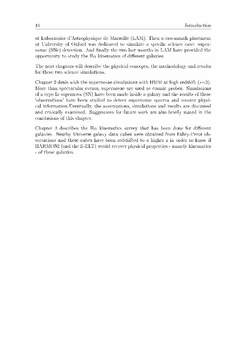
Chapter 2 deals with the supernovae simulations with HSIM at high redshift (z∼3).More than spectacular events, supernovae are used as cosmic probes. Simulationsof a type Ia supernova (SN) have been made inside a galaxy and the results of theseòbservations' have been studied to detect supernovae spectra and recover physi-cal information.Eventually, the assumptions, simulations and results are discussedand critically examined. Suggestions for future work are also briey stated in theconclusions of this chapter.

Chapter 3 describes the Hα kinematics survey that has been done for dierentgalaxies. Nearby Universe galaxy data cubes were obtained from Fabry-Perot ob-servations and these cubes have been redshifted to a higher z in order to know ifHARMONI (and the E-ELT) would recover physical properties - namely kinematics- of these galaxies.

Supernovae project 11

Chapter 2

Supernovae project

In this chapter, we present the supernovae project, whereby we simulate observationsof a type Ia SN in a galaxy at z∼3 with HSIM, in order to recover the SN type fordierent intrinsic luminosities. We introduce SN physics, describe the simulationassumptions and procedures, and present the result and analysis for this study.

2.1 Supernovae physics

In 1054, when people observed a very bright event for many months in the sky theythought it could be a new star, similar to the Sun. In fact it was not the birth of astar, but on the contrary its death: the result of the dramatic explosion of a massivestar. Nowadays we have a better idea of what happened to the now so-called CrabNebula (Figure 2.1). Indeed, massive stars undergo many nuclear chain reactionsthat burn hydrogen and produce heavier elements up to iron, which has the greatestbinding energy. Thus the stellar core collapses due to its own gravity and forms aneutron core. A violent expulsion of the outer layers of the star ensues: massivestars (with masses greater than ∼ 10 solar masses) have a very intense life andsupernovae are their last stellar evolutionary stage.

2.1.1 Supernovae classication

Supernovae are classied according to their spectrum (Filipenko et al. 1997 [3]).There are two supernova types: type I and type II. The lack of hydrogen lines inthe type I spectrum allows to dierentiate both types.Among hydrogen-decient supernovae, we can theoretically distinguish three sub-types: SNe Ia are characterized by a deep absorption at 6150 Å produced by silicon,SNe Ib show helium lines (especially at λ=5876 Å) and SNe Ic present neither siliconnor helium lines. Types Ib, Ic and II SNe are the result of the core collapse processpreviously described. SNe Ia are due to another phenomena: the accretion of matter

12 Supernovae project

Figure 2.1: Crab Nebula or M1 is a supernova remnant: the SN exploded in 1054and ejected material still expands at a speed of 1500 km/s. Credit Hubble SpaceTelescope.

onto a white dwarf from a companion. A white dwarf is a dense hot stellar core thatslowly cools. When it reaches the Chandrasekhar limit, the critical mass equal to1.4 solar masses, this is the tipping point: the white dwarf explodes in a type Ia SN.

Whatever the physical reason, a supernova explosion leads to a cataclysmic explo-sion, and matter is expelled away from the star at velocities up to 30000 km/s (10%of the speed of light). This matter is called the SN remnant and these cosmic debrisare composed of chemical elements from the nuclear fusion. More than contributingto the heavy element production which forms the Universe (and subsequently hu-mankind), the remnant helps unravel the nuclear physics of supernovae and thus thestellar explosion process. SN spectra and light-curves are therefore very importantto observe.

Light-curves display the magnitude of the supernova versus time. The integratedspectrum over a bandpass lter gives the magnitude at a specic time and thesephotometric measurements allow one to plot dierent points on the light-curve be-fore, after and at maximum light. Whereas for type I, the shape of the light-curvesis very similar, the type II SNe have a much dispersed curve and we can classifythree subtypes on the basis of their downslope: type II-n (for `normal'), type II-p(for `plateau') and type II-l (for `linear'). Light-curves for types Ia, Ib, II-l and II-pare shown in Figure 2.2.

Supernovae are exceptionally bright events and can briey outshine an entire galaxy.Only one or two stellar explosions occur in a century in galaxies such as the MilkyWay. Nevertheless, astronomers needed "standard candles" to quantify the accel-eration of the Universe. Perlmutter [7] denes these standard candles as àny dis-


Figure 2.2: Schematic light curves for SNe of types Ia, Ib, II-L, II-P, and SN 1987A.The curve for SNe Ib includes SNe Ic as well, and represents an average. For SNe II-L, SNe 1979C and 1980K are used, but these might be unusually luminous. Note thattype I SNe have a similar shape but type Ia has a higher average peak luminosity.Credit (Filipenko et al. 1997 [3]).

tinguishable class of astronomical objects of known intrinsic brightness that can beidentied over a wide distance range'.

2.1.2 SNe Ia as standard candles

At the end of the previous century, the Supernova Cosmology Project, a researchteam in Berkeley found out that distant SNe Ia were actually dimmer than theirlocal counterparts, meaning these SNe were farther away than expected (Perlmutter2003 [7]). This was evidence that the acceleration of the Universe was not decel-erating as one thought but on the contrary accelerating. In this way theoreticalphysicists start to put the pieces of the cosmological puzzle back together by recon-sidering the `cosmological constant' introduced by Einstein in his theory of generalrelativity. This expansionary term corresponding to the negative pressure compo-nent of the Universe plants the seed for a dark energy explanation.


Since then, SNe Ia seem to be a strong cosmic probe (Branch et al. [1]). Indeed,dierent arguments can be put forward in favour of type Ia for measuring the valueof the accelerating expansion by demonstrating the dilation of the light curves ofhigh-redshift SNe. The redshift z is completely dened by ∆λ/λ, where ∆λ is thespectral stretch of the λ wavelength. One of the most important argument for SNeIa as cosmic probes is their spectral homogeneity as Figure 2.3 shows. Indeed, mostof the type Ia spectra look very similar with strong features at λ= 6150 Å (Si II)and at λ = 3934 and 3968 Å (Ca II H&K).

Figure 2.3: Spectra of SNe Ia about one week past maximum brightness. The parentgalaxies and their redshifts (kilometers per second) are as follows: SN 1990N (NGC4639; 970), SN 1987N (NGC7606; 2171), and SN 1987D (MCG+00-32-01; 2227).Credit (Filipenko et al, 1997).

Another signicant reason for the use of SNe Ia being standard candles is the verycharacteristic light-curve shape and the common maximum brightness for this type.As a matter of fact Figure 2.4 explains how it is possible to correct light-curveswith a stretch factor in order to have a perfectly uniform shape for all SNe Ia. Themeasurement of their initial maximum brightness attests their distance from Earthby dealing with redshift and thus can reveal the way the Universe has expanded.


Figure 2.4: Light curves of nearby, low-redshift type Ia supernovae measured byMario Hamuy and coworkers. (a) Absolute magnitude, an inverse logarithmic mea-sure of intrinsic brightness, is plotted against time (in the star's rest frame) beforeand after peak brightness. The great majority (not all of them shown) fall neatlyonto the yellow band. The gure emphasizes the relatively rare outliers whose peakbrightness or duration diers noticeably from the norm. The nesting of the lightcurves suggests that one can deduce the intrinsic brightness of an outlier from itstime scale. The brightest supernovae wax and wane more slowly than the faintest.(b) Simply by stretching the time scales of individual light curves to t the norm,and then scaling the brightness by an amount determined by the required timestretch, one gets all the type Ia light curves to match. Credit (Perlmutter 2003 [7]).

The frenzied hunt for supernovae has begun and if 8-meter-class telescopes gaveaccess to half the age of the Universe, astronomers expect that E-ELT and JWST


will observe SNe beyond a redshift of four, which corresponds to 90% of the age ofthe Universe.

2.2 SN-Ia simulations inside a galaxy

The main goal of this project is to simulate SNe Ia inside a galaxy at z∼3 for dif-ferent luminosities and to observe what the E-ELT would be able to observe. Thiswill give a limiting magnitude, i.e. the magnitude beyond which the SN cannot bedetected anymore and the simulation has lost the information about the SN type.

In this study, the input galaxy is taken from the output of a large-scale cosmologicalsimulation. Physics of galaxies has been adequately understood to simulate veryrealistic data and then generate galaxies of suciently high spatial resolution. Theseare ideal for spatially resolved simulations with HARMONI.

2.2.1 Magnitude calculations for the host galaxy

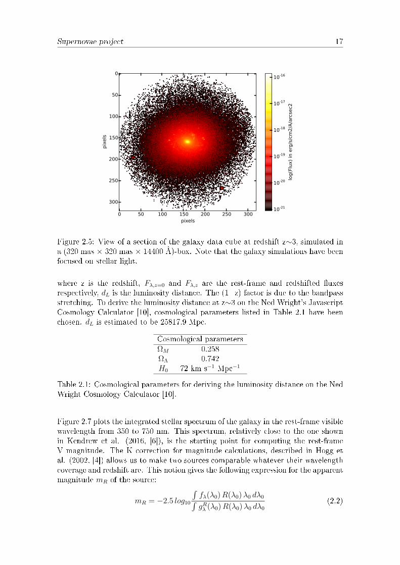
The input galaxy simulations have been performed with the code RAMSES to givestellar population data from which star particles have been converted into stellarlight.The input data cube (x, y, λ) has a size of (320, 320, 4000) and contains a 10-kpc galaxy (Figure 2.5) redshifted at z∼3. Its covers the 1.44-2.88 µm wavelengthrange and the spectral sampling is 3.6 Å, while the spectral resolution is equal to10 Å. Regarding the spatial dimension, the data cube has been sampled on a 1 x1 mas grid of spaxels. Therefore the mock galaxy is a data cube of size 320 mas ×320 mas. Figure 2.6 plots the spatially integrated spectrum of the galaxy at z∼3.Note that the galaxy simulations have been focused on stellar absorption lines (forreasons independent of the present study) leading to a spectrum with no emissionlines. The near-infrared H and K bands correspond to 1.45-1.85 µm and 1.9-2.4 µmrespectively, they are shaded in orange and red on the gure. Both will be used aslters for the SNe observations.

Prior to any simulations, the magnitude of the host galaxy needs to be preciselyknown and for this purpose, the galaxy is de-redshifted and the magnitude in therest-frame V-band is computed and compared to a previous study on the same galaxy(Kendrew et al. 2016 [6]). In this way, one is condent in the calibration of thegalaxy ux and in the ratio between supernova luminosity and galaxy luminosity.Galaxies at high redshift are observed to be fainter than their local counterparts.This is called the cosmological dimming. The spectral sampling (and resolution)will be divided by (1+z) and the ux can be calculated with the following equation:

Fλ,z=0 = Fλ,z (dL

10pc)2 (1 + z) (2.1)


0 50 100 150 200 250 300pixels

0

50

100

150

200

250

300

pixels

10-21

10-20

10-19

10-18

10-17

10-16

log(Flux) in erg/s/cm2/A/arcse

c2

Figure 2.5: View of a section of the galaxy data cube at redshift z∼3, simulated ina (320 mas × 320 mas × 14400 Å)-box. Note that the galaxy simulations have beenfocused on stellar light.

where z is the redshift, Fλ,z=0 and Fλ,z are the rest-frame and redshifted uxesrespectively, dL is the luminosity distance. The (1+z) factor is due to the bandpassstretching. To derive the luminosity distance at z∼3 on the Ned Wright's JavascriptCosmology Calculator [10], cosmological parameters listed in Table 2.1 have beenchosen. dL is estimated to be 25817.9 Mpc.

Cosmological parametersΩM 0.258ΩΛ 0.742H0 72 km s−1 Mpc−1

Table 2.1: Cosmological parameters for deriving the luminosity distance on the NedWright Cosmology Calculator [10].

Figure 2.7 plots the integrated stellar spectrum of the galaxy in the rest-frame visiblewavelength from 350 to 750 nm. This spectrum, relatively close to the one shownin Kendrew et al. (2016, [6]), is the starting point for computing the rest-frameV magnitude. The K correction for magnitude calculations, described in Hogg etal. (2002, [4]) allows us to make two sources comparable whatever their wavelengthcoverage and redshift are. This notion gives the following expression for the apparentmagnitude mR of the source:

mR = −2.5 log10

∫fλ(λ0)R(λ0)λ0 dλ0∫gRλ (λ0)R(λ0)λ0 dλ0

(2.2)


14000 16000 18000 20000 22000 24000 26000 28000 30000Wavelength in Angstroms

2

3

4

5

6

7Fl

ux in e

rg/s

/cm

2/A

1e 20 Integrated flux from RAMSES simulations at z=3

H-bandK-band

Figure 2.6: Integrated stellar spectra of the z=3 RAMSES galaxy between 1.44 and2.88 µm. Note that the galaxy simulations have been focused on stellar absorptionlines (no emission lines). The near-infrared H and K bands corresponding to 1.45-1.85 µm and 1.9-2.4 µm respectively have been shaded in orange and red.

where the integrals are over the observed wavelengths λ0; fλ(λ0) is the spectral den-sity ux (energy per unit time per unit area per unit wavelength); gRλ is the spectraldensity of ux for the zero-magnitude or `standard' source, which in this case isVega (see Table 2.2) and R(λ0) is the bandpass. The smaller the magnitude, thebrighter the celestial object.

From the spectrum in Figure 2.7, calculations of the rest-frame V-band magnitudegives -21.28 (Kendrew et al. (2016 [6]) found -21.4 for the same simulated galaxy).At z∼3 the apparent magnitude of the galaxy is equal to +23.3 in the H-band and+22.4 in the K-band. Integrated spectrum and magnitude calculations have beencomputed for a galaxy aperture size of 10 kpc. At z∼3 the galaxy is at an angularsize distance of 1613.6 Mpc which gives a scale of 0.127 "/kpc and thus occupies atotal 1.27 " eld.

After having derived the magnitude, the ux of the host galaxy is intrinsically knownand one can simulate a supernova as a fraction of this luminosity. The next step



0.6

0.8

1.0

1.2

1.4

1.6

1.8Fl

ux in e

rg/s

/cm

2/A

Integrated flux from RAMSES simulationsin the rest-frame visible wavelength

V-band

Figure 2.7: Integrated stellar spectra of of the galaxy in rest-frame between 350and 750 nm. The optical V band corresponding to 450-700 nm has been shaded inpurple.

is to estimate the total ux that a local supernova should have when redshifted toz∼3.

2.2.2 SNe magnitude calibrations

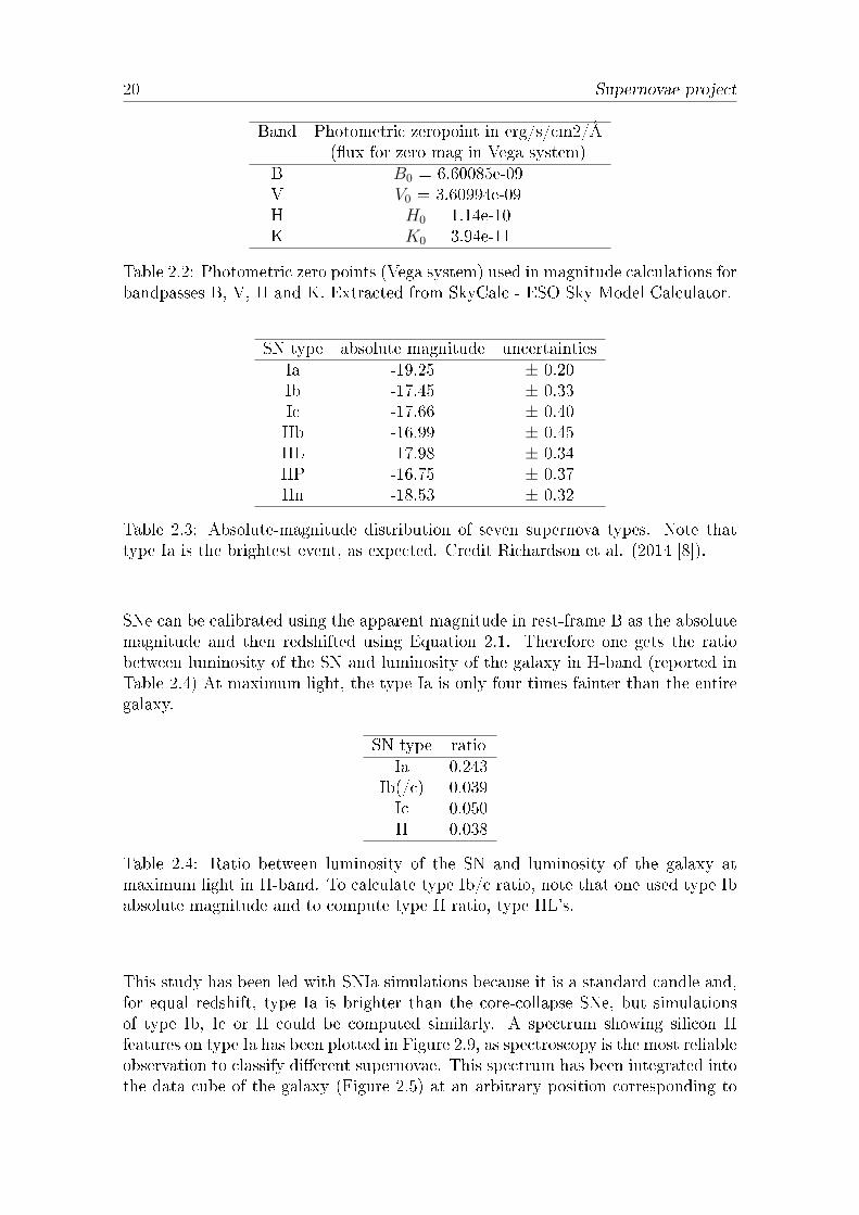
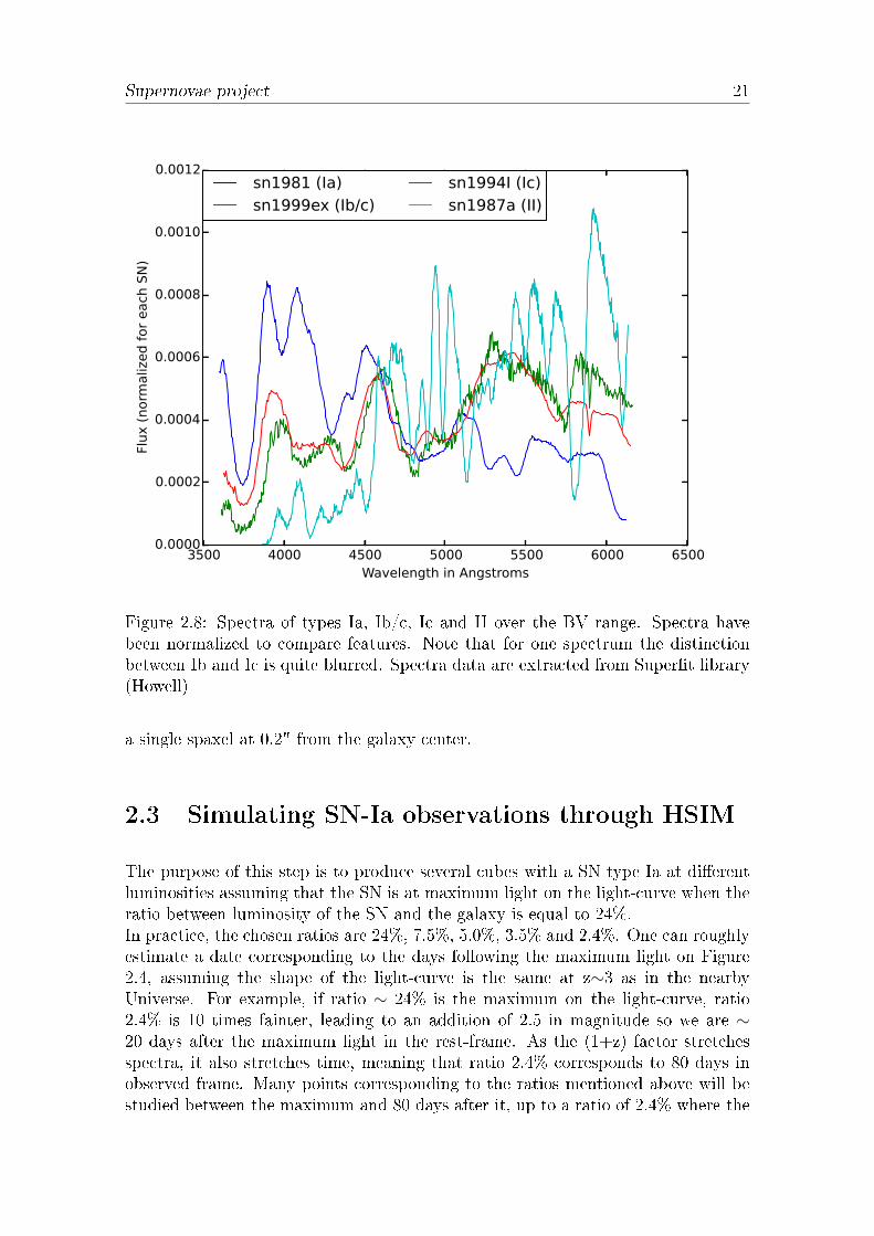
It has been shown that distant supernovae were fainter than their local counterparts(Perlmutter et al. 2003 [7]). This is evidence of cosmological dimming. In thecontext of this study, relatively local SNe will be redshifted at z∼3 by scaling theirspectra. Richardson et al. (2014 [8]) presents the absolute-magnitude distributionof seven supernova types (Table 2.3). The absolute magnitude is the magnitudethat a celestial object would have if it were located at a standard distance of 10pc from Earth (∼ 1014 kms). Spectra for types Ia, Ib/c, Ic and II are shown inFigure 2.8 for the 350-600 nm range (BV band). These SNe have been observedin the nearby Universe at maximum light and are extracted from Supert library(Howell, http://www.dahowell.com/superfit.html): Ia corresponds to SN1981,Ib/c to SN1999EX, Ic to SN1994I and II to SN1987A.

At z∼3, the H-band corresponds to the rest-frame B; this means that the ux of

http://www.dahowell.com/superfit.html


Band Photometric zeropoint in erg/s/cm2/Å(ux for zero mag in Vega system)

B B0 = 6.60085e-09V V0 = 3.60994e-09H H0 = 1.14e-10K K0 = 3.94e-11

Table 2.2: Photometric zero points (Vega system) used in magnitude calculations forbandpasses B, V, H and K. Extracted from SkyCalc - ESO Sky Model Calculator.

SN type absolute magnitude uncertaintiesIa -19.25 ± 0.20Ib -17.45 ± 0.33Ic -17.66 ± 0.40IIb -16.99 ± 0.45IIL -17.98 ± 0.34IIP -16.75 ± 0.37IIn -18.53 ± 0.32

Table 2.3: Absolute-magnitude distribution of seven supernova types. Note thattype Ia is the brightest event, as expected. Credit Richardson et al. (2014 [8]).

SNe can be calibrated using the apparent magnitude in rest-frame B as the absolutemagnitude and then redshifted using Equation 2.1. Therefore one gets the ratiobetween luminosity of the SN and luminosity of the galaxy in H-band (reported inTable 2.4) At maximum light, the type Ia is only four times fainter than the entiregalaxy.

SN type ratioIa 0.243

Ib(/c) 0.039Ic 0.050II 0.038

Table 2.4: Ratio between luminosity of the SN and luminosity of the galaxy atmaximum light in H-band. To calculate type Ib/c ratio, note that one used type Ibabsolute magnitude and to compute type II ratio, type IIL's.

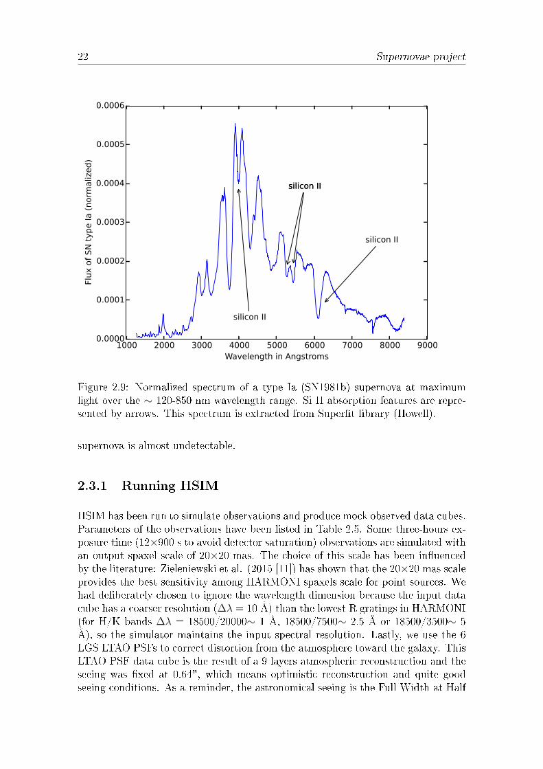
This study has been led with SNIa simulations because it is a standard candle and,for equal redshift, type Ia is brighter than the core-collapse SNe, but simulationsof type Ib, Ic or II could be computed similarly. A spectrum showing silicon IIfeatures on type Ia has been plotted in Figure 2.9, as spectroscopy is the most reliableobservation to classify dierent supernovae. This spectrum has been integrated intothe data cube of the galaxy (Figure 2.5) at an arbitrary position corresponding to


3500 4000 4500 5000 5500 6000 6500Wavelength in Angstroms

0.0000

0.0002

0.0004

0.0006

0.0008

0.0010

0.0012

Flux (norm

alized for each SN)

sn1981 (Ia)sn1999ex (Ib/c)

sn1994I (Ic)sn1987a (II)

Figure 2.8: Spectra of types Ia, Ib/c, Ic and II over the BV range. Spectra havebeen normalized to compare features. Note that for one spectrum the distinctionbetween Ib and Ic is quite blurred. Spectra data are extracted from Supert library(Howell)

a single spaxel at 0.2" from the galaxy center.

2.3 Simulating SN-Ia observations through HSIM

The purpose of this step is to produce several cubes with a SN type Ia at dierentluminosities assuming that the SN is at maximum light on the light-curve when theratio between luminosity of the SN and the galaxy is equal to 24%.In practice, the chosen ratios are 24%, 7.5%, 5.0%, 3.5% and 2.4%. One can roughlyestimate a date corresponding to the days following the maximum light on Figure2.4, assuming the shape of the light-curve is the same at z∼3 as in the nearbyUniverse. For example, if ratio ∼ 24% is the maximum on the light-curve, ratio2.4% is 10 times fainter, leading to an addition of 2.5 in magnitude so we are ∼20 days after the maximum light in the rest-frame. As the (1+z) factor stretchesspectra, it also stretches time, meaning that ratio 2.4% corresponds to 80 days inobserved frame. Many points corresponding to the ratios mentioned above will bestudied between the maximum and 80 days after it, up to a ratio of 2.4% where the



0.0000

0.0001

0.0002

0.0003

0.0004

0.0005

0.0006

Flux of SN type Ia (norm

alized)

silicon II

silicon IIsilicon II

silicon II

Figure 2.9: Normalized spectrum of a type Ia (SN1981b) supernova at maximumlight over the ∼ 120-850 nm wavelength range. Si II absorption features are repre-sented by arrows. This spectrum is extracted from Supert library (Howell).

supernova is almost undetectable.

2.3.1 Running HSIM

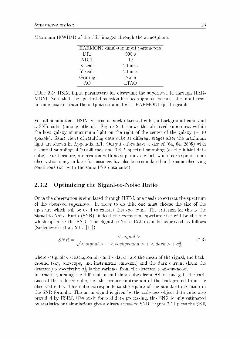
HSIM has been run to simulate observations and produce mock observed data cubes.Parameters of the observations have been listed in Table 2.5. Some three-hours ex-posure time (12×900 s to avoid detector saturation) observations are simulated withan output spaxel scale of 20×20 mas. The choice of this scale has been inuencedby the literature: Zieleniewski et al. (2015 [11]) has shown that the 20×20 mas scaleprovides the best sensitivity among HARMONI spaxels scale for point sources. Wehad deliberately chosen to ignore the wavelength dimension because the input datacube has a coarser resolution (∆λ = 10 Å) than the lowest R gratings in HARMONI(for H/K bands ∆λ = 18500/20000∼ 1 Å, 18500/7500∼ 2.5 Å or 18500/3500∼ 5Å), so the simulator maintains the input spectral resolution. Lastly, we use the 6LGS LTAO PSFs to correct distortion from the atmosphere toward the galaxy. ThisLTAO PSF data cube is the result of a 9 layers atmospheric reconstruction and theseeing was xed at 0.64", which means optimistic reconstruction and quite goodseeing conditions. As a reminder, the astronomical seeing is the Full Width at Half


Maximum (FWHM) of the PSF imaged through the atmosphere.

HARMONI simulator input parametersDIT 900 sNDIT 12X scale 20 masY scale 20 masGrating NoneAO LTAO

Table 2.5: HSIM input parameters for observing the supernova Ia through HAR-MONI. Note that the spectral dimension has been ignored because the input reso-lution is coarser than the outputs obtained with HARMONI spectrograph.

For all simulations, HSIM returns a mock observed cube, a background cube anda SNR cube (among others). Figure 2.10 shows the observed supernova withinthe host galaxy at maximum light on the right of the center of the galaxy (∼ 10spaxels). Same views of resulting data cube at dierent stages after the maximumlight are shown in Appendix A.1. Output cubes have a size of (64, 64, 2805) witha spatial sampling of 20×20 mas and 3.6 Å spectral sampling (as the initial datacube). Furthermore, observation with no supernova, which would correspond to anobservation one year later for instance, has also been simulated in the same observingconditions (i.e. with the same PSF data cube).

2.3.2 Optimizing the Signal-to-Noise Ratio

Once the observation is simulated through HSIM, one needs to extract the spectrumof the observed supernova. In order to do this, one must choose the size of theaperture which will be used to extract this spectrum. The criterion for this is theSignal-to-Noise Ratio (SNR); indeed the extraction aperture size will be the onewhich optimise the SNR. The Signal-to-Noise Ratio can be expressed as follows(Zieleniewski et al. 2015 [11]):

SNR =< signal >√

< signal > + < background > + < dark > +σ2R

(2.3)

where <signal>, <background> and <dark> are the mean of the signal, the back-ground (sky, telescope, and instrument emission) and the dark current (from thedetector) respectively; σ2

R is the variance from the detector read-out-noise.In practice, among the dierent output data cubes from HSIM, one gets the vari-ance of the reduced cube, i.e. the proper subtraction of the background from theobserved cube. This cube corresponds to the square of the standard deviation inthe SNR formula. The mean signal is given by the noiseless object data cube alsoprovided by HSIM. Obviously for real data processing, this SNR is only estimatedby statistics but simulations give a direct access to SNR. Figure 2.11 plots the SNR


0 10 20 30 40 50 60pixels

0

10

20

30

40

50

60

pixels

10-4

10-3

10-2

10-1

100

101

102

log(Flux) in erg/s/cm2/A/arcse

c2

Figure 2.10: View of the observed data cube with the supernova within the hostgalaxy at maximum light, obtained by calculating the median for each spaxel of thesky-subtracted data cube. The SNIa has been simulated at 0.2" on the right of thecenter of the galaxy, namely 10 spaxels.

at maximum light for several aperture sizes centered on the supernova location.Calculations have been carried out for dierent wavelengths between 1.45 and 2.45µm. To avoid galaxy contamination, the galaxy data cube one year later has beensubtracted from the observations with the supernova. This operation adds noiseto the galaxy observation. The gure suggests that extracting the supernova in a2×2-spaxel box, namely a 40×40 mas box yields the best SNR whatever the wave-length. Note that there is no general trend to increase or decrease the SNR plot asa function of wavelength, this may be due to the emission and absorption lines ofthe sky or nebula which result in enhanced photon noise at specic λ. The shape ofthe SNR curve can be explained by the fact that at the beginning an increase of thebox size gathers more signal from the object but the noise becomes more importantonce we cross a specic size (here 2×2 spaxels) .

From the literature, one learns that we may be condent that for SNR > 5 andthe smaller the error on the magnitude (error on magnitude ∼ ( S

N)−1). To increase

it, we can choose to increase the exposure time, because SNR∼√t but one can

easily imagine that the observation time is limited for each science case. Anotherway to do that is to rebin the spectral dimension. Indeed, in the SNR formula(Equation 2.3) if we make the rough assumption that the photon noise is the mainsource of noise, we are left with signal ∼ N and noise ∼

√N and then SNR ∼

√N .

By rebinning the wavelength dimension with C pixels, we increase the number ofphotons and thus the SNR by a factor

√C. In doing so, we lose in resolution but we


1 2 3 4 5 6 7 8Linear size of square box (in pixels)

0.2

0.4

0.6

0.8

1.0

1.2

1.4

1.6

1.8

2.0Signal-to-Noise Ratio

Wavelength

1440.0 nm1620.0 nm1800.0 nm1980.0 nm2160.0 nm2340.0 nm

Figure 2.11: Signal-to-Noise Ratio at maximum light for several aperture sizes (inpixels) centered on the supernova location. Calculations have been performed fordierent wavelengths between 1.45 and 2.45 µm. To avoid galaxy contamination, anobservation of the galaxy one year later has been subtracted from the observationincluding the supernova. Note that this operation adds noise.

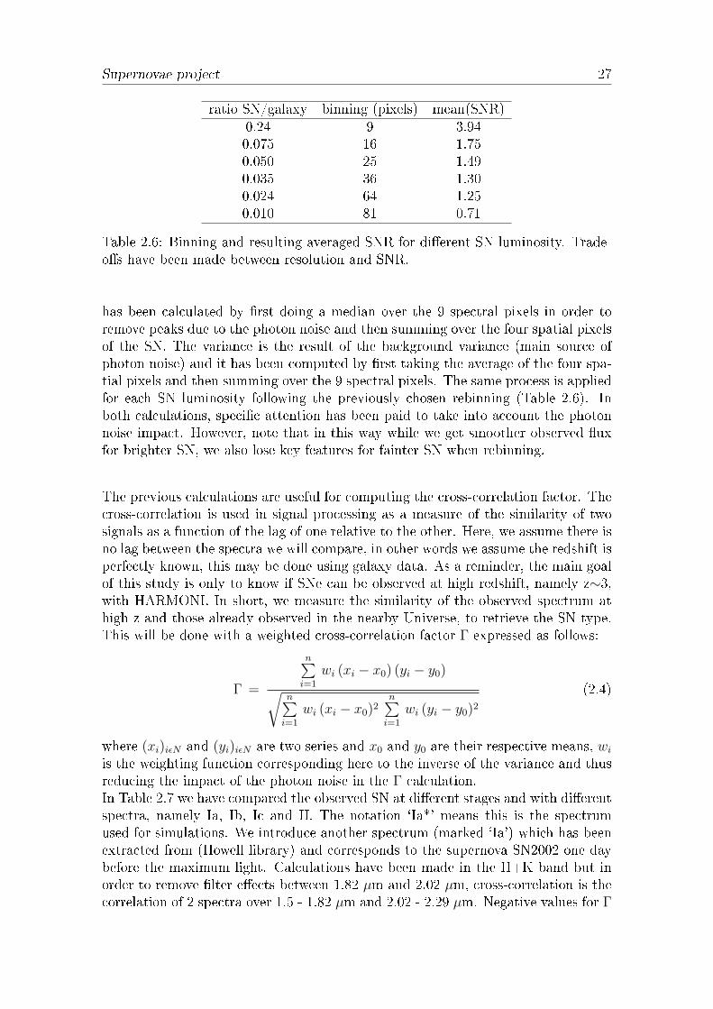
gain in reliability. In this study, the input data has a coarser resolution (∆λ ∼ 10Å) than the HARMONI resolution. Hence we can bin the spectral dimension, carebeing taken not to degrade the resolution too much because we want to be able todetect spectral features. For this, we choose to bin the maximum light spectrum by9 pixels, so that the mean SNR of the maximum light is multiplied by ∼ 3 (Figure2.12). For each dierent luminosity ratio, we have made trade-os between the SNRand the resolution. The chosen binning and the resulting mean SNR are listed inTable 2.6 while the impact on SNR of rebinning is shown in Appendix A.2 for allstages.

In a nutshell, to have exploitable data, we have needed to optimize the aperture sizeand the SNR of spectra. Trade-os have been made to increase the SNR withoutlosing too much resolution. In the next section, spectra are extracted to get themost reliable information from data and to classify supernova Ia. Note that thesame process could be conducted to analyze any of the supernovae types.


1.4 1.6 1.8 2.0 2.2 2.4 2.6Wavelength in nm

0

2

4

6

8

10

12

14

16Signal-to-Noise Ratio

no spectral binningspectral binning (9 pixels)

Figure 2.12: Signal-to-Noise Ratio at maximum light for the wavelength range 1.45to 2.45 µm in 3 hours. The blue curve is the result of a 10 Å spectral resolution whilefor the green one we have degraded the spectral dimension to 90 Å to increase theSNR and give more condence to the output signal. Galaxy has not been subtracted.

2.4 Supernovae classication

Supernovae classication has to be made from a study of the spectrum becauselight-curves cannot help to do the distinction between dierent type Is, except atequal redshift where SNe Ia are supposed to have the highest maximum. Hence thespectral analysis stands as the most reliable tool for classication. In the followingwe choose to focus on two methods for data analysis: the cross-correlation and theχ2 methods.

2.4.1 Cross-Correlation method

Once the aperture size and the SNR are optimized, we can extract the spectrumof the supernova for data processing. Figures 2.13 and Appendix A.3 display theextracted spectrum and the associated background variance of SN at maximum lightand for ratios 0.075, 0.050, 0.035 and 0.024 respectively. As previously mentioned,the aperture is a 40×40 mas box. In the case of maximum light, the spectral ux


ratio SN/galaxy binning (pixels) mean(SNR)0.24 9 3.940.075 16 1.750.050 25 1.490.035 36 1.300.024 64 1.250.010 81 0.71

Table 2.6: Binning and resulting averaged SNR for dierent SN luminosity. Trade-os have been made between resolution and SNR.

has been calculated by rst doing a median over the 9 spectral pixels in order toremove peaks due to the photon noise and then summing over the four spatial pixelsof the SN. The variance is the result of the background variance (main source ofphoton noise) and it has been computed by rst taking the average of the four spa-tial pixels and then summing over the 9 spectral pixels. The same process is appliedfor each SN luminosity following the previously chosen rebinning (Table 2.6). Inboth calculations, specic attention has been paid to take into account the photonnoise impact. However, note that in this way while we get smoother observed uxfor brighter SN, we also lose key features for fainter SN when rebinning.

The previous calculations are useful for computing the cross-correlation factor. Thecross-correlation is used in signal processing as a measure of the similarity of twosignals as a function of the lag of one relative to the other. Here, we assume there isno lag between the spectra we will compare, in other words we assume the redshift isperfectly known, this may be done using galaxy data. As a reminder, the main goalof this study is only to know if SNe can be observed at high redshift, namely z∼3,with HARMONI. In short, we measure the similarity of the observed spectrum athigh z and those already observed in the nearby Universe, to retrieve the SN type.This will be done with a weighted cross-correlation factor Γ expressed as follows:

Γ =

n∑i=1

wi (xi − x0) (yi − y0)√n∑i=1

wi (xi − x0)2n∑i=1

wi (yi − y0)2

(2.4)

where (xi)iεN and (yi)iεN are two series and x0 and y0 are their respective means, wiis the weighting function corresponding here to the inverse of the variance and thusreducing the impact of the photon noise in the Γ calculation.In Table 2.7 we have compared the observed SN at dierent stages and with dierentspectra, namely Ia, Ib, Ic and II. The notation Ìa*' means this is the spectrumused for simulations. We introduce another spectrum (marked Ìa') which has beenextracted from (Howell library) and corresponds to the supernova SN2002 one daybefore the maximum light. Calculations have been made in the H+K band but inorder to remove lter eects between 1.82 µm and 2.02 µm, cross-correlation is thecorrelation of 2 spectra over 1.5 - 1.82 µm and 2.02 - 2.29 µm. Negative values for Γ


14000 16000 18000 20000 22000 24000 26000Lambda (Angstroms)

200

0

200

400

600

800Fl

ux (

ele

ctro

ns)

Observed SN


100000

300000

500000

Flux (

ele

ctro

ns)

Variance

Figure 2.13: Extracted spectrum and associated background variance at maximumlight with a rebinning of 9 pixels. The H and K bands are shaded in orange and redrespectively. Galaxy has not been subtracted.

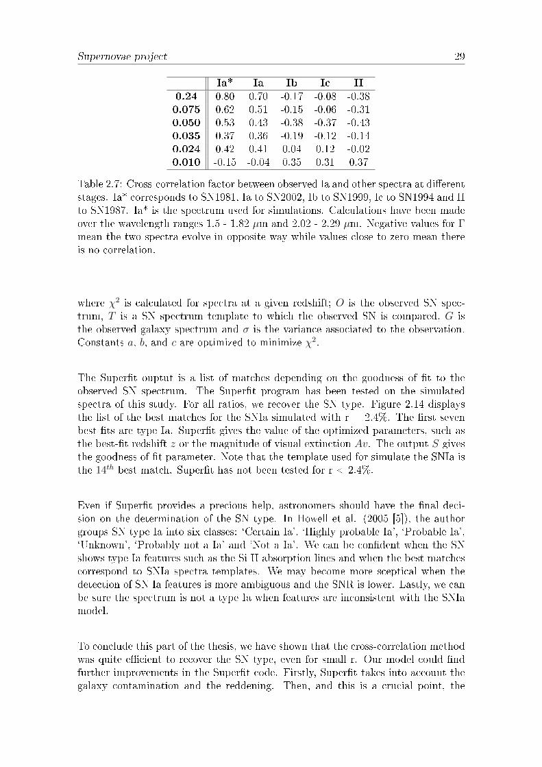
mean the two spectra evolve in opposite ways while values close to zero mean thereis no correlation. The cross-correlation yields the highest value for both type Ia andis far superior to the others types up to r = 0.024. From this ratio onward, the SNtype is undetectable and extracting a spectrum mismatches the SN type.

2.4.2 Minimum χ2 method and conclusions

The χ2 method is the tting method used in Supert, IDL software written by AndyHowell to nd the best match to an observed spectrum from a library of hundreds ofpreviously observed spectra of SNe. In Howell et al. (2005 [5]), the author explainshow to compute χ2 to try to minimize it and thus recover the SN type. χ2 dependson three parameters: the redshift z, the amount of galaxy contamination and thereddening law Aλ. The reddening is due to the extinction of light by dust and gasand because blue light is more absorbed than red light, stellar objects appear redder.As a consequence, χ2 is calculated as follows:

χ2 =∑λ

[O(λ) − aT (λ, z)10cAλ − bG(λ, z)]2

σ(λ)2(2.5)


Ia* Ia Ib Ic II0.24 0.80 0.70 -0.17 -0.08 -0.380.075 0.62 0.51 -0.15 -0.06 -0.310.050 0.53 0.43 -0.38 -0.37 -0.430.035 0.37 0.36 -0.19 -0.12 -0.140.024 0.42 0.41 0.04 0.12 -0.020.010 -0.15 -0.04 0.35 0.31 0.37

Table 2.7: Cross-correlation factor between observed Ia and other spectra at dierentstages. Ia* corresponds to SN1981, Ia to SN2002, Ib to SN1999, Ic to SN1994 and IIto SN1987. Ia* is the spectrum used for simulations. Calculations have been madeover the wavelength ranges 1.5 - 1.82 µm and 2.02 - 2.29 µm. Negative values for Γmean the two spectra evolve in opposite way while values close to zero mean thereis no correlation.

where χ2 is calculated for spectra at a given redshift; O is the observed SN spec-trum, T is a SN spectrum template to which the observed SN is compared, G isthe observed galaxy spectrum and σ is the variance associated to the observation.Constants a, b, and c are optimized to minimize χ2.

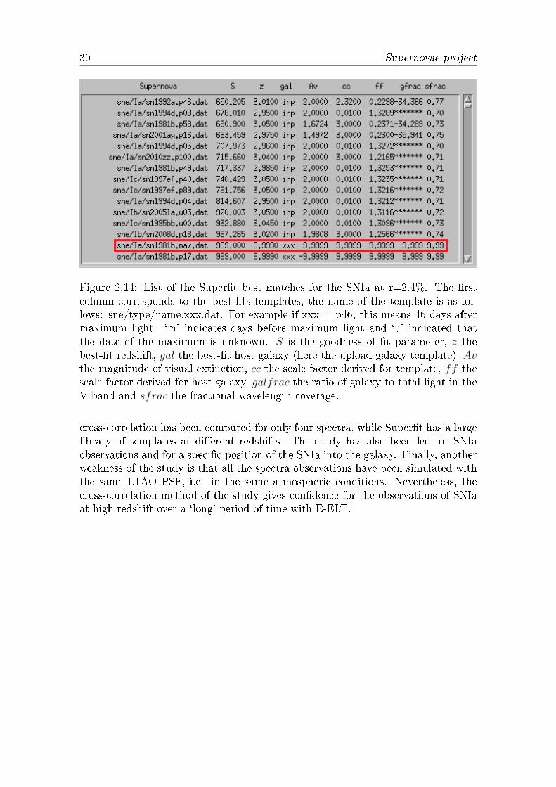
The Supert ouptut is a list of matches depending on the goodness of t to theobserved SN spectrum. The Supert program has been tested on the simulatedspectra of this study. For all ratios, we recover the SN type. Figure 2.14 displaysthe list of the best matches for the SNIa simulated with r = 2.4%. The rst sevenbest ts are type Ia. Supert gives the value of the optimized parameters, such asthe best-t redshift z or the magnitude of visual extinction Av. The output S givesthe goodness of t parameter. Note that the template used for simulate the SNIa isthe 14th best match. Supert has not been tested for r < 2.4%.

Even if Supert provides a precious help, astronomers should have the nal deci-sion on the determination of the SN type. In Howell et al. (2005 [5]), the authorgroups SN type Ia into six classes: `Certain Ia', `Highly probable Ia', `Probable Ia',Ùnknown', `Probably not a Ia' and `Not a Ia'. We can be condent when the SNshows type Ia features such as the Si II absorption lines and when the best matchescorrespond to SNIa spectra templates. We may become more sceptical when thedetection of SN Ia features is more ambiguous and the SNR is lower. Lastly, we canbe sure the spectrum is not a type Ia when features are inconsistent with the SNIamodel.

To conclude this part of the thesis, we have shown that the cross-correlation methodwas quite ecient to recover the SN type, even for small r. Our model could ndfurther improvements in the Supert code. Firstly, Supert takes into account thegalaxy contamination and the reddening. Then, and this is a crucial point, the


Figure 2.14: List of the Supert best matches for the SNIa at r=2.4%. The rstcolumn corresponds to the best-ts templates, the name of the template is as fol-lows: sne/type/name.xxx.dat. For example if xxx = p46, this means 46 days aftermaximum light. `m' indicates days before maximum light and ù' indicated thatthe date of the maximum is unknown. S is the goodness of t parameter, z thebest-t redshift, gal the best-t host galaxy (here the upload galaxy template), Avthe magnitude of visual extinction, cc the scale factor derived for template, ff thescale factor derived for host galaxy, galfrac the ratio of galaxy to total light in theV band and sfrac the fractional wavelength coverage.

cross-correlation has been computed for only four spectra, while Supert has a largelibrary of templates at dierent redshifts. The study has also been led for SNIaobservations and for a specic position of the SNIa into the galaxy. Finally, anotherweakness of the study is that all the spectra observations have been simulated withthe same LTAO PSF, i.e. in the same atmospheric conditions. Nevertheless, thecross-correlation method of the study gives condence for the observations of SNIaat high redshift over a `long' period of time with E-ELT.

Hα kinematic survey of galaxies 31

Chapter 3

Hα kinematic survey of galaxies

In this chapter, we present the work that has been performed to build a pipeline fora Hα kinematic survey of galaxies using a pre-existing software, called Camel. Firstwe introduce the context of this survey and the input data used. Then, we describehow the observation of galaxies has been simulated with HSIM. Eventually, all thedata processing is explained from HSIM outputs to the use of the Camel code whichgives velocity eld used to plot the rotation curves of the studied galaxies.

3.1 Hα kinematics and input data

A previous kinematic survey (Epinat et al. 2008 [2]) was made in the local Universefrom Fabry-Perot observations on the almost 2-meter telescope in Observatoire deHaute Provence (France), as part of the Gassendi HAlpha survey of SPirals (GHASPsurvey). This survey has gathered 3D data cubes of spiral and irregular galaxies,around the Hα line. The main goal of the present study is to use these nearbyUniverse galaxies and redshift them at higher z to simulate the observations withHARMONI and compare the rotation curves at a coarser spatial resolution to theones found in the local Universe. As an introduction, we present Fabry-Perot inter-ferometry, Hα line and input data cubes for HSIM.

3.1.1 Hα kinematics

At the beginning of the 20th century, Fabry and Perot used for the very rst timean interferometer to observe solar lines. Nowadays, the Fabry-Perot interferometeris used as a spectrally resolving instrument. Indeed, just as in a laser cavity theFabry-Perot interferometer is made of two semi-reecting mirrors which produceconstructive and destructive interferences while light comes into the cavity and isreected from one surface to the other. The resonance is reached by constructive

32 Hα kinematic survey of galaxies

interferences at specic wavelengths and, as a consequence, the transmission spec-trum of the interferometer shows peaks of large transmission at these wavelengths.Constructive interferences occur for λ described in Equation 3.1 where p is an inte-ger, n is the refractive index of the medium between the two mirrors, e the distancebetween the two mirrors and θ is the angle between the incident light and the op-tical axis. By tunning the spacing between mirrors, the Fabry-Perot interferometeris able to scan a part of the spectrum and we thus get a broader range of wavelengths.

λ =2n e

pcos(Θ) (3.1)

Kinematics is the study of the relative motion of matter inside galaxies. In this sur-vey, Hα kinematics of galaxies have been studied, this means that we have observedthe shift of the Hα line inside each galaxy to get the velocity of stellar matter as a2D map of the galaxy. Velocity eld maps are computed using the Doppler-Fizeaueect. Hα is one of the emission lines from atomic transition of hydrogen, calledthe Balmer series, corresponding to 656.3 nm in the rest-frame. This emission lineis particularly tracked by astronomers because it is a feature of many nebulae: it isvery intense in comparison to other emission lines, and hence leads to a higher SNR.The ionized hydrogen will be used as a probe to compute kinematics of galaxies inorder to link kinematics to the properties of galaxies. By reducing data, we will beable to derive 2D Hα map, 2D rotation velocity eld map and 1D rotation curve foreach galaxy.

3.1.2 Input data cubes for HSIM

As in the supernova project, inputs are data cubes with two spatial dimensions andone spectral dimension. The main dierence is that input cubes are real data fromobservations. The Fabry-Perot interferometer was able to observe about 200 galax-ies with IFS. In the frame of the GHASP survey, high spectral resolution 3D datacubes in the vicinity of the Hα line have been obtained, giving a Hα prole for eachpixel of the FoV.

In this study, we decide to redshift the set of galaxies at z∼1.4, which correspondsto an angular size distance of distz∼1.4 ∼ 1767.3 Mpc (Ned Wright CosmologicalCalculator). At this redshift, we choose to observe galaxies with the HARMONIspaxel scales of 20×20 mas and 30×60 mas. Thus the next step is to choose onlygalaxies which will have a better input spatial resolution than these output spaxelscales. The resolution of the input galaxies is completely limited by the seeing of theobservations. This selection is made by calculating the input redshifted resolution:

resz∼1.4 =resz∼0 × distz∼0

distz∼1.4

(3.2)


where resz∼0 and resz∼1.4 are the input spatial resolution at z∼0 and z∼ 1.4 re-spectively, distz∼0 and distz∼1.4 are the angular size distance at z∼0 and z∼ 1.4respectively. Whereas distz∼1.4 is equal to 1767.3 Mpc, distz∼0 is around 10 Mpcand the seeing is arount 3". Thus resz∼1.4 needs to be smaller than 20 mas. Amongthe 200 galaxies of the GHASP survey, 45 galaxies satisfy this criterion and arelisted in Appendix B.1 with their respective local distance, initial seeing, redshiftedspatial resolution and FoV. Concerning the spectral dimension, we have a set of datawith a spectral resolution of R∼9000 which gives ∆λ ∼ 6563/9000 = 0.73 Å.Once the galaxies selection has been done, we prepare data cubes for HSIM. Basi-cally we chop the spatial dimensions in order to centre the data cube on the galaxycentre thanks to the right ascension α and the declination δ of the rotation centre.Then we check that data cubes have the required headers with the accepted values(see Table 1.1). As part of this step, we remind that HSIM only takes into input awavelength dimension, so we had to convert the third dimension which was initiallyexpressed as a velocity, into wavelength using formula of the Doppler-Fizeau eect:

∆λ = λg∆v

c(3.3)

λg = λ0 (1 + zg) (3.4)

zg =vsysc

(3.5)

where ∆λ and ∆v are the wavelength and velocity samplings respectively, λg is theglobal wavelength of the galaxy at redshift zg, and vsys and c are the global velocityof the galaxy and the speed of light respectively.The inputs preparation also redshifts data cubes at z∼ 1.4 which stretches the spec-trum by a factor (1+z). The ux is then modied. Indeed, the spectrum ux isintegrated spatially and spectrally in order to calibrate the Hα prole to get a totalux of the emission line of 5×10−16 erg/s/cm2 for the spatial scale of 20×20 masand a total ux of 10−16 erg/s/cm2 for the spatial scale of 30×60 mas in order toensure a sucient SNR once projected at higher z.

In this report, the galaxy UGC 7045 has been chosen to display all the data pro-cessing performed. Figure 3.1 shows the galaxy before running HSIM, computed byaveraging the spectral dimension. The logarithmic scale emphasizes the ux varia-tion. The redshifted spatial resolution is equal to 13.6 mas (and spatial sampling isequal to 4.3 mas) and the observation covers a FoV of 2.06". The black line givesthe direction of the major-axis.

3.2 Observing galaxies with HSIM and data pro-

cessing with Camel

The HARMONI Simulator and the Camel code have been run for the 45 galaxieslisted in Appendix B.1, each time for two output spaxel scales.


0 100 200 300 400pixels

0

100

200

300

400

pixels

10-21

10-20

10-19

10-18

10-17

10-16

10-15

Flux (erg/s/cm2/A/arcse

c2)

Figure 3.1: Galaxy UGC 7045 before running HSIM, computed by averaging thespectral dimension. The logarithmic scale emphasizes the ux variation. The red-shifted spatial resolution is equal to 13.6 mas and the observation covers a FoV of2.06". The black line gives the direction of the major-axis.

3.2.1 Running HSIM

Table 3.1 gathers the parameters used for the simulation of the observation of thegalaxies at redshift of z∼1.4. Some 2-hour exposure time observations have beensimulated for both spaxel scales. The same PSF than the one upload in the Super-nova project has been used while the ouput spectral resolution has been chosen toR = 7500 leading to ∆λ = 6563× (1+z)

7500∼ 2.1 Å . Figure 3.2 shows the reduced cube

(background subtracted to observation) of galaxy UGC 7045 after running HSIMfor the 20×20 mas scale. The PSF convolution has created a halo around the galaxy.


HARMONI simulator input parametersDIT 900 sNDIT 8X scale 20 mas/30 masY scale 20 mas/60 masGrating H (R = 7500)AO LTAO

Table 3.1: HSIM input parameters for observing the 45 galaxies through HARMONI.Note that the PSF used is the same upload PSF than in the Supernova project.

0 20 40 60 80 100pixels

0

20

40

60

80

100

pixels

10-3

10-2

10-1

100

101

102

103

Flux (electrons)

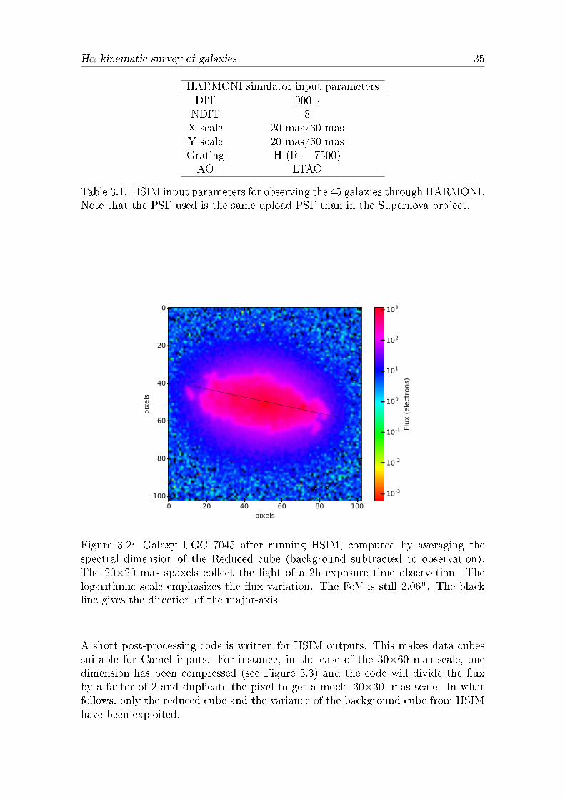
Figure 3.2: Galaxy UGC 7045 after running HSIM, computed by averaging thespectral dimension of the Reduced cube (background subtracted to observation).The 20×20 mas spaxels collect the light of a 2h exposure time observation. Thelogarithmic scale emphasizes the ux variation. The FoV is still 2.06". The blackline gives the direction of the major-axis.

A short post-processing code is written for HSIM outputs. This makes data cubessuitable for Camel inputs. For instance, in the case of the 30×60 mas scale, onedimension has been compressed (see Figure 3.3) and the code will divide the uxby a factor of 2 and duplicate the pixel to get a mock `30×30' mas scale. In whatfollows, only the reduced cube and the variance of the background cube from HSIMhave been exploited.


0 10 20 30 40 50 60pixels

0

5

10

15

20

25

30

pixels

10-1

100

101

102

Flux (electrons)

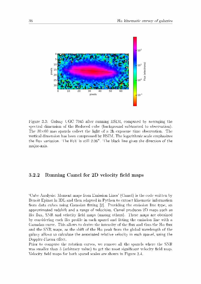
Figure 3.3: Galaxy UGC 7045 after running HSIM, computed by averaging thespectral dimension of the Reduced cube (background subtracted to observation).The 30×60 mas spaxels collect the light of a 2h exposure time observation. Thevertical dimension has been compressed by HSIM. The logarithmic scale emphasizesthe ux variation. The FoV is still 2.06". The black line gives the direction of themajor-axis.

3.2.2 Running Camel for 2D velocity eld maps

`Cube Analysis: Moment maps from Emission Lines' (Camel) is the code written byBenoit Epinat in IDL and then adapted in Python to extract kinematic informationfrom data cubes using Gaussian tting [2]. Providing the emission line type, anapproximated redshift and a range of velocities, Camel produces 2D maps such asHα ux, SNR and velocity eld maps (among others). These maps are obtainedby considering each Hα prole in each spaxel and tting the emission line with aGaussian curve. This allows to derive the intensity of the ux and thus the Hα uxand the SNR maps, as the shift of the Hα peak from the global wavelength of thegalaxy allows to calculate the associated relative velocity in each spaxel, using theDoppler-Fizeau eect.Prior to compute the rotation curves, we remove all the spaxels where the SNRwas smaller than 5 (arbitrary value) to get the most signicant velocity eld map.Velocity eld maps for both spaxel scales are shown in Figure 3.4.


0 20 40 60 80 100pixels

0

20

40

60

80

100

pix

els

20 mas sampling

−120

−80

−40

0

40

80

120

160

km/s

0 10 20 30 40 50 60pixels

0

10

20

30

40

50

60

pix

els

30 mas sampling

−120

−80

−40

0

40

80

120

km/s

Figure 3.4: Velocity eld maps of the galaxy UGC 7045 for two spaxel scales: 20×20mas (left) and 30×60 mas (right). The 20 mas sampling covers a larger FoV (for SNR> 5) than the 30 mas sampling and as expected, the 20 mas sampling shows moredetails on the velocity eld map. Black lines give the direction of the major-axis.

3.2.3 Rotation curves

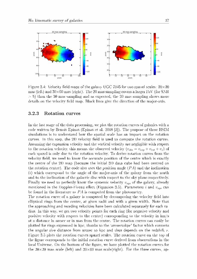
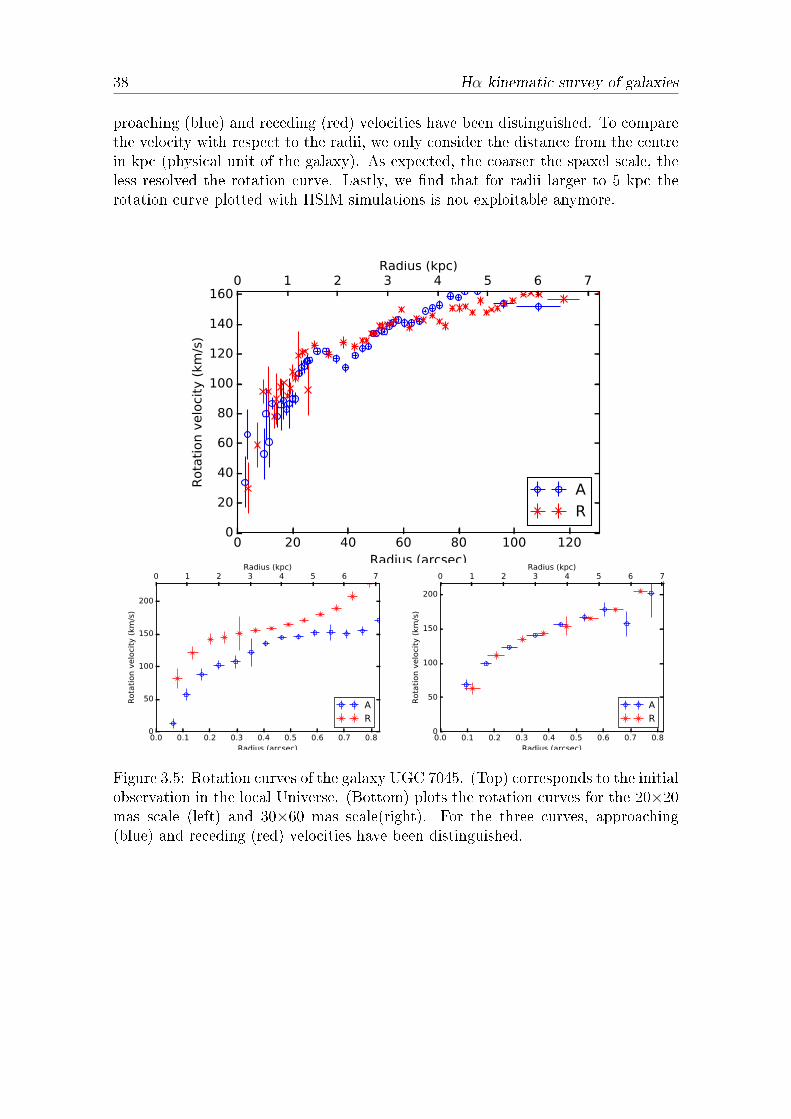
In the last stage of the data processing, we plot the rotation curves of galaxies with acode written by Benoit Epinat (Epinat et al. 2008 [2]). The purpose of these HSIMsimulations is to understand how the spatial scale has an impact on the rotationcurves. In this step, the 2D velocity eld is used to compute the rotation curves.Assuming the expansion velocity and the vertical velocity are negligible with respectto the rotation velocity, this means the observed velocity (vobs = vexp + vrot + vz) ofeach spaxel is only due to the rotation velocity. To derive rotation curves from thevelocity eld, we need to know the accurate position of the centre which is exactlythe centre of the 2D map (because the initial 3D data cube had been centred onthe rotation centre). The code also uses the position angle (PA) and the inclination(i) which correspond to the angle of the major-axis of the galaxy from the northand to the inclination of the galactic disc with respect to the sky plane respectively.Finally we need to perfectly know the systemic velocity vsys of the galaxy, alreadymentioned in the Doppler-Fizeau eect (Equation 3.5). Parameters i and vsys canbe found in the literature as PA is computed from the photometry.The rotation curve of a galaxy is computed by decomposing the velocity eld intoelliptical rings from the centre, at given radii and with a given width. Note thatthe approaching and receding velocities have been calculated separately for each ra-dius. In this way, we get two velocity points for each ring (for negative velocity andpositive velocity with respect to the centre) corresponding to the velocity in km/sat a distance in arcsec or in mas from the centre. The rotation curves can easily beplotted for rings expressed in kpc, thanks to the àrcsectokpc' factor which convertsthe angular size distance from arcsec to kpc and thus depends on the redshift z.Figure 3.5 plots the rotation curves spaxel scales. The rotation curve on the top ofthe gure corresponds to the initial rotation curve derived from observations in thelocal Universe. On the bottom of the gure, we have plotted the rotation curves forthe 20×20 mas scale (left) and 30×60 mas scale(right). For the three curves, ap-


proaching (blue) and receding (red) velocities have been distinguished. To comparethe velocity with respect to the radii, we only consider the distance from the centrein kpc (physical unit of the galaxy). As expected, the coarser the spaxel scale, theless resolved the rotation curve. Lastly, we nd that for radii larger to 5 kpc therotation curve plotted with HSIM simulations is not exploitable anymore.

0 20 40 60 80 100 120Radius (arcsec)

0

20

40

60

80

100

120

140

160

Rotation velocity (km

/s)

0 1 2 3 4 5 6 7Radius (kpc)

AR

0.0 0.1 0.2 0.3 0.4 0.5 0.6 0.7 0.8Radius (arcsec)

0

50

100

150

200


/s)

0 1 2 3 4 5 6 7Radius (kpc)

AR

0.0 0.1 0.2 0.3 0.4 0.5 0.6 0.7 0.8Radius (arcsec)

0

50

100

150

200


/s)

0 1 2 3 4 5 6 7Radius (kpc)

AR

Figure 3.5: Rotation curves of the galaxy UGC 7045. (Top) corresponds to the initialobservation in the local Universe. (Bottom) plots the rotation curves for the 20×20mas scale (left) and 30×60 mas scale(right). For the three curves, approaching(blue) and receding (red) velocities have been distinguished.

Conclusion 39

Chapter 4

Conclusion

In this thesis, we have introduced the 39-m E-ELT and HARMONI IFS concepts.HSIM is the simulation pipeline for HARMONI simulations. It can predict whatthe IFS performance would be. In this concern, we have simulated the observationof two celestial objects, which have already been observed in the local universe butnot at higher redshift.Firstly, the supernovae project has shown that E-ELT and HARMONI will be ableto observe for redshift of 3, supernovae Ia for many days after maximum-light (forsmall r in the study). The cross-correlation has given quite good results to recoverthe type of the simulated SNe, but as stated at the end of the Chapter 2, the modelis really simplistic and needs to be improved.Secondly, the Hα kinematics survey of 45 galaxies at redshift of 1.4 has been initi-ated. Simulations of the observation of spatially resolved galaxies have been madewith HSIM in order to study the Hα kinematics of each galaxy. Then rotation curveshave been plotted from velocity eld maps for dierent spaxel scales of HARMONI.The purpose of this study was to see the impact of the resolution on rotation curves,and thus to predict the rotation curves that we will obtain with HARMONI IFS forgalaxies of earlier times.

From a personal perspective, this master thesis has been an incredible experience.Taking part to such a prestigious project was a chance for me and I really appreci-ated the work I got to do. Once again I discovered new elds in astrophysics and itkeeps becoming more and more fascinating.

40 REFERENCES

References

[1] D. Branch. Type Ia Supernovae as Standard Candles. Annu. Rev. Astron.Astrophys., 1992.

[2] B. Epinat, P. Amram, M. Marcelin, C. Balkowski, O. Daigle, O. Hernandez,and L. Chemin et al. GHASP : An Hα kinematic survey of spiral and irregulargalaxies. Monthly Notices of the Royal Astronomical Society, 2008.

[3] A.V. Filippenko. Optical Spectra of Supernovae. Annu. Rev. Astron.Astrophys., 1997.

[4] D.W. Hogg, I.K. Baldry, M.R. Blanton, and D.J. Eisenstein. The K correction.arXiv:astro-ph/0210394, 2002.

[5] D. A. Howell, M. Sullivan, K. Perrett, T. J. Bronder, I. M. Hook, P. Astier,and E. Aubourg et al. Gemini Spectroscopy of Supernovae from the SupernovaLegacy Survey: Improving High-Redshift Supernova Selection and Classica-tion. The Astrophysical Journal, 2005.

[6] S. Kendrew, S. Zieleniewski, R.C.W. Houghton, N. Thatte, J. Devriendt, andM. Tecza et al. Simulated stellar kinematics studies of high-redshift galaxieswith the HARMONI Integral Field Spectrograph. Monthly Notices of the RoyalAstronomical Society, 2016.

[7] S. Perlmutter. Supernovae, Dark Energy, and the Accelerating Universe.American Institute of Physics, 2003.

[8] D. Richardson, R. L. Jenkins III, J. Wright, and L. Maddox. Absolute-Magnitude Distributions of Supernovae. arXiv:1403.5755, 2014.

[9] N. A. Thatte, F. Clarke, I. Bryson, H. Schnetler, M. Tecza, R. M. Bacon, andA. Remillieux et al. HARMONI: the rst light integral eld spectrograph forthe E-ELT. SPIE, 2014.

[10] E. L. Wright. A Cosmology calculator for the World Wide Web. ThePublications of the Astronomical Society of the Pacic, 2006.

[11] S. Zieleniewski, N. Thatte, S. Kendrew, R. C. W. Houghton, A. M. Swinbank,M. Tecza, F. Clarke, and T. Fusco. HSIM: a simulation pipeline for the HAR-MONI integral eld spectrograph on the European ELT. Monthly Notices ofthe Royal Astronomical Society, 2015.

References 41

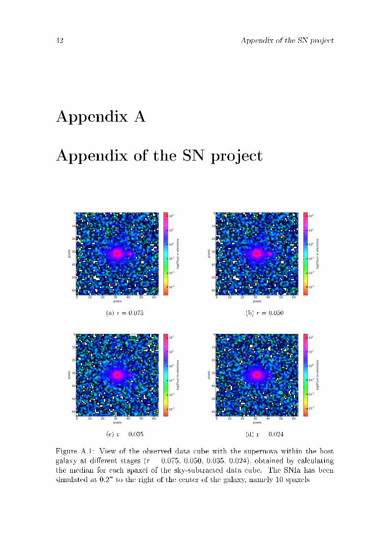
42 Appendix of the SN project

Appendix A

Appendix of the SN project

0 10 20 30 40 50 60pixels

0

10

20

30

40

50

60

pixels

10-3

10-2

10-1

100

101

102

log(Flux) in electrons

(a) r = 0.075

0 10 20 30 40 50 60pixels

0

10

20

30

40

50

60

pixels

10-3

10-2

10-1

100

101

102


(b) r = 0.050

0 10 20 30 40 50 60pixels

0

10

20

30

40

50

60

pixels

10-3

10-2

10-1

100

101

102


(c) r = 0.035

0 10 20 30 40 50 60pixels

0

10

20

30

40

50

60

pixels

10-3

10-2

10-1

100

101

102


(d) r = 0.024

Figure A.1: View of the observed data cube with the supernova within the hostgalaxy at dierent stages (r = 0.075, 0.050, 0.035, 0.024), obtained by calculatingthe median for each spaxel of the sky-subtracted data cube. The SNIa has beensimulated at 0.2" to the right of the center of the galaxy, namely 10 spaxels

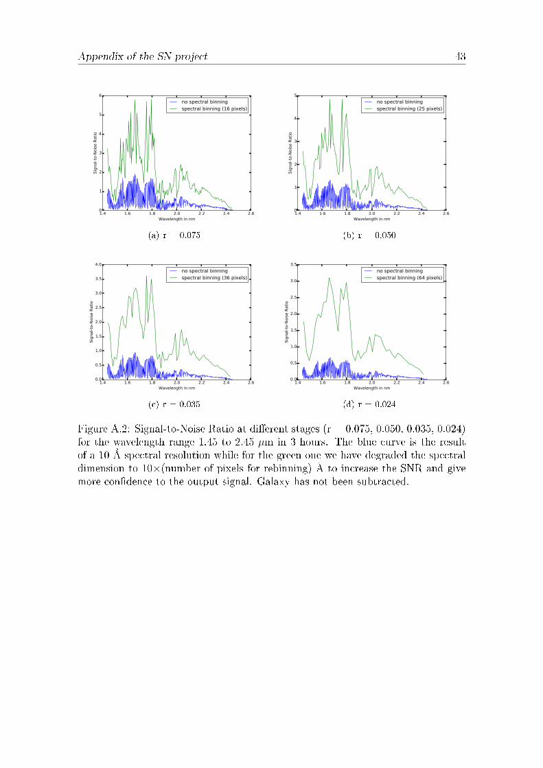
Appendix of the SN project 43

1.4 1.6 1.8 2.0 2.2 2.4 2.6Wavelength in nm

0

1

2

3

4

5

6Sig

nal-

to-N

ois

e R

ati

o


(a) r = 0.075

1.4 1.6 1.8 2.0 2.2 2.4 2.6Wavelength in nm

0

1

2

3

4

5

Sig

nal-

to-N

ois

e R

ati

o


(b) r = 0.050

1.4 1.6 1.8 2.0 2.2 2.4 2.6Wavelength in nm

0.0

0.5

1.0

1.5

2.0

2.5

3.0

3.5

4.0

Sig

nal-

to-N

ois

e R

ati

o


(c) r = 0.035

1.4 1.6 1.8 2.0 2.2 2.4 2.6Wavelength in nm

0.0

0.5

1.0

1.5

2.0

2.5

3.0

3.5

Sig

nal-

to-N

ois

e R

ati

o


(d) r = 0.024

Figure A.2: Signal-to-Noise Ratio at dierent stages (r = 0.075, 0.050, 0.035, 0.024)for the wavelength range 1.45 to 2.45 µm in 3 hours. The blue curve is the resultof a 10 Å spectral resolution while for the green one we have degraded the spectraldimension to 10×(number of pixels for rebinning) Å to increase the SNR and givemore condence to the output signal. Galaxy has not been subtracted.

44 Appendix of the SN project


300

200

100

0

100

200

300

400

Flux (

ele

ctro

ns)

Observed SN


0

100000

200000

300000

400000

500000

600000

700000

800000

Flux (

ele

ctro

ns)

Variance

(a) r = 0.075


200150100

500

50100150200250

Flux (

ele

ctro

ns)

Observed SN


0

200000

400000

600000

800000

1000000

1200000

Flux (

ele

ctro

ns)

Variance

(b) r = 0.050


150

100

50

0

50

100

150

200

250

Flux (

ele

ctro

ns)

Observed SN


0

200000

400000

600000

800000

1000000

1200000

1400000

Flux (

ele

ctro

ns)

Variance

(c) r = 0.035


40

20

0

20

40

60

80

100

Flux (

ele

ctro

ns)

Observed SN


0

500000

1000000

1500000

2000000

2500000

Flux (

ele

ctro

ns)

Variance

(d) r = 0.024

Figure A.3: Extracted spectrum and associated background variance for dierentratios (r = 0.075, 0.050, 0.035, 0.024) between SN luminosity and galaxy luminosity.Appropriate rebinning has been done for each luminosity. The H and K bands areshaded in orange and red respectively. Galaxy has not been subtracted.

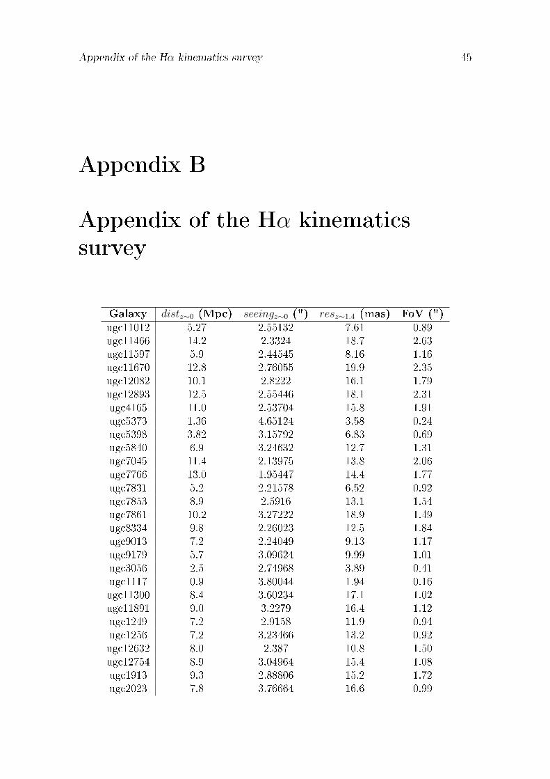
Appendix of the Hα kinematics survey 45

Appendix B

Appendix of the Hα kinematics

survey

Galaxy distz∼0 (Mpc) seeingz∼0 (") resz∼1.4 (mas) FoV (")ugc11012 5.27 2.55132 7.61 0.89ugc11466 14.2 2.3324 18.7 2.63ugc11597 5.9 2.44545 8.16 1.16ugc11670 12.8 2.76055 19.9 2.35ugc12082 10.1 2.8222 16.1 1.79ugc12893 12.5 2.55446 18.1 2.31ugc4165 11.0 2.53704 15.8 1.91ugc5373 1.36 4.65124 3.58 0.24ugc5398 3.82 3.15792 6.83 0.69ugc5840 6.9 3.24632 12.7 1.31ugc7045 11.4 2.13975 13.8 2.06ugc7766 13.0 1.95447 14.4 1.77ugc7831 5.2 2.21578 6.52 0.92ugc7853 8.9 2.5916 13.1 1.54ugc7861 10.2 3.27222 18.9 1.49ugc8334 9.8 2.26023 12.5 1.84ugc9013 7.2 2.24049 9.13 1.17ugc9179 5.7 3.09624 9.99 1.01ugc3056 2.5 2.74968 3.89 0.41ugc1117 0.9 3.80044 1.94 0.16ugc11300 8.4 3.60234 17.1 1.02ugc11891 9.0 3.2279 16.4 1.12ugc1249 7.2 2.9158 11.9 0.94ugc1256 7.2 3.23466 13.2 0.92ugc12632 8.0 2.387 10.8 1.50ugc12754 8.9 3.04964 15.4 1.08ugc1913 9.3 2.88806 15.2 1.72ugc2023 7.8 3.76664 16.6 0.99

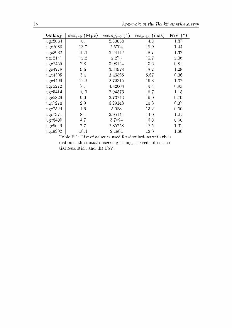
46 Appendix of the Hα kinematics survey

Galaxy distz∼0 (Mpc) seeingz∼0 (") resz∼1.4 (mas) FoV (")ugc2034 10.1 2.50038 14.3 1.37ugc2080 13.7 2.5704 19.9 1.44ugc2082 10.2 3.24142 18.7 1.32ugc2141 12.2 2.278 15.7 2.06ugc2455 7.8 3.08154 13.6 0.81ugc4278 9.6 3.34928 18.2 1.28ugc4305 3.4 3.46566 6.67 0.36ugc4499 12.2 2.79815 19.3 1.32ugc5272 7.1 4.82608 19.4 0.85ugc5414 10.0 2.94576 16.7 1.15ugc5829 9.0 3.73743 19.0 0.70ugc7278 2.9 6.29148 10.3 0.37ugc7524 4.6 5.088 13.2 0.50ugc7971 8.4 2.95144 14.0 1.01ugc8490 4.7 3.7694 10.0 0.60ugc9649 7.7 2.85758 12.5 1.31ugc9992 10.4 2.1964 12.9 1.80

Table B.1: List of galaxies used for simulations with theirdistance, the initial observing seeing, the redshifted spa-tial resolution and the FoV.

Documents

AIX MARSEILLE UNIVERSITE ECOLE CENTRALE DE …doc.centrale-marseille.fr/TFE/inter2016/Bounissou_Sophie_Rapport.pdf · HSIM HARMONI Simulator i inclination IFS Integral Field Spectroscopy