Alcohol Prohibition and Infant Mortality1 Alcohol Prohibition and Infant Mortality Briggs Depew Louisiana State University [email protected] Griffin Edwards University of Alabama at Birmingham

1

Alcohol Prohibition and Infant Mortality

Briggs Depew

Louisiana State University

[email protected]

Griffin Edwards

University of Alabama at

Birmingham

[email protected]

Emily Owens

University of Pennsylvania

[email protected]

This Draft: Aug 1st, 2013

Abstract

The merits of alcohol prohibition have been, and continue to be heavily debated. While the net

effect of alcohol prohibition on violence is uncertain, one clear potential positive externality to

alcohol prohibition is improved health outcomes, through improved prenatal health, reduced

domestic violence, and/or higher standards of living. These effects should be especially salient

among expecting mothers, birth outcomes for infants, and young children in general. Using data

on age specific mortalities and exploiting the variation of state level prohibition laws, we

estimate alcohol prohibition’s impact on mortality rates from internal causes (sickness,

congenital disorder) and external causes (violence, neglect, accidents) for infants and young

children. We find a reduction in the share of infants under the age of one who die of internal

causes rather than external causes when the commercial sale of alcohol is criminalized. We find

that the reduction in the number of deaths for children aged one through nine is the result of

prohibition’s effect on external causes of death.

2

I. Introduction

State sponsored policies banning certain types of goods, services and behaviors have

been, and continues to be, and important public policy topic. Alcohol prohibition in the early

20th century was the most prominent and stark ban on a consumable good. Many policy makers

today still refer back to that “noble experiment” as an example of the efficacy (or inefficacy) of a

wide sweeping ban. Until recently, however, there has been presented very little evidence of any

direct and/or indirect effect of Prohibition.

Recent work has shown that the heaviest of alcohol consumers, those who suffer from

liver cirrhosis, probably consumed less alcohol during Prohibition (Miron and Dills 2004), that

the volume of alcohol produced (or smuggled) and thus available for consumption decreased

even to the average consumer (Edwards and Howe 2013), and that while there is little evidence

that the overall level of crime increased in response to Prohibition, there was a disproportionate

increase in crime to those most likely to participate in illegal markets (Owens 2013). One of the

most important policy considerations that accompany the analysis of Prohibition is the health

effects that result from a ban on alcohol consumption. While there is some evidence of the effect

of Prohibition on alcohol consumers (Miron and Dills 2004), the externalities of alcohol

consumption are non-trivial (e.g. Cook and Moore 2012). To date, there is no direct evidence on

health outcomes for people who are non-drinkers, but lived in close proximity to potential

drinkers during the American Temperance Movement.

If Prohibition was truly effective in decreasing alcohol consumption, and alcohol does

indeed have negative effects on third parties, one of the groups that stood to gain the most from

Prohibition were young children; specifically those who were conceived and born to parents

3

whose alcohol consumption was eliminated, or significantly decreased, when commercial

alcohol sales were criminalized. A child born in a dry state could potentially be healthier

through two avenues. First, she should be healthier because of improved maternal health in

utero. A mother who does not drink during pregnancy is much more likely to give birth to a

healthy baby (Currie 2011). It could also be the case, however, that the health of the child

improved as a result of a change in the composition of the family. As discussed in greater detail

in the next section, male alcohol consumption was commonly seen at the time as a safety issue

for women and children, as social norms limited both labor market opportunities and legal status

for women (Geddes and Tennyson 2013). Thus, children may have also experienced gains to

health as a result of increased family income, and reduced violence or stress in the household.

There is some evidence that marginal changes to alcohol control policies1 can be an effective

tool in improving health outcomes (Markowitz and Grossman 1998), particularly to mothers and

infants (Fertig and Watson 2009), but an outright ban on alcohol is much more grand and a very

different policy than contemporary control policies, and there is no cleaner policy “experiment”

than Prohibition.

The aim of this work is to identify the extent and the potential channels through which

children benefited from an “alcohol free,” or at least “alcohol reduced,” environment. Are the

gains to health for children a result from improved maternal health during pregnancy, the result

of less violence in the home, or a combination of both? To our knowledge, no other work has

attempted to empirically answer this question through the study of alcohol prohibition. Our work

provides insight into the short-run implications of the American Temperance Movement. Using

1 For example, an increase in the beer tax or change in minimum legal drinking age.

4

an alternative approach in studying state prohibition laws, Ferreira, Marks, and Sorensen (2012)

study the long-run labor market outcomes of individuals born in dry states.

To understand the interaction of state level alcohol prohibition policies on immediate

health outcomes of infants and children, we collected census data on the cause of death by age,

and exploit the variation in state dry laws that were passed prior to Federal Prohibition. We

consider infants that died due to internal bodily reasons a measure of maternal health while

infants that died due to external causes (e.g. violence, neglect)2 to be a measure of changes in the

composition of the household. However, given the data limitations, it is difficult to sort out the

extent of these channels. For example, through prohibition, family income may have been

substituted away from alcohol and to increases in health and care in the home. In general, we

find that the proportion of infants that died due to internal causes of death decreased by about 2.5

percentage points in states with dry laws. For older children we find the opposite effect,

specifically, the proportion of deaths from internal causes increases, suggesting that decreases in

external causes is the dominant force.

II. Prohibition Laws and Child Health

The “noble experiment” of Federal Prohibition, which lasted from 1920 to 1932, had its roots

in the Second Great Awakening in 1790. A unique feature of this particular religious social

movement was the involvement of women who played an important role in shaping the central

issues of the associated groups (Gusfield 1986, Szymanski 2003). Due, at least in part, to the

expanded role of women in the Great Awakening, groups like the Woman’s Christian

Temperance Union and the American Temperance Society were focused on improving the

2 A precise definition of each is given the Appendix

5

wellbeing of children and families through proselytizing; encouraging poor, immigrant, and non-

white men to behave according to Protestant standards of behavior, which included prayer,

regular church attendance, vigorous physical exercise, and temperate use of alcohol (Szymanski

2003). Alcohol consumption was seen as a male activity that directly harmed families by

reducing the income available for food, rent, and clothing.3

Men’s alcohol consumption was also portrayed as a safety issue; women and children had

little legal or social protection if husbands were neglectful or violent with them.4 Consistent with

this, surveys of household expenditures in “working class families” often contain reports of men

hiding their alcohol expenditure from their wives, with surveyors having the question husbands

in isolation in order to estimate true consumption levels.5

Analyses of contemporary alcohol control policies seem to confirm the point in that it

suggests that tightening alcohol control policies tend to reduce domestic violence (Markowitz

and Grossman 1998) specifically to children (Shen 2006). Additionally, increased access to

alcohol through lenient minimum legal drinking age laws increased unplanned pregnancies, and

are associated with worse birth outcomes (Fertig and Watson 2009).

Temperance organizations promoted their behavioral ideas in a number of ways, including

holding prayer meetings in from of local saloons, publishing textbooks describing the deleterious

health effects of alcohol consumption, and also promoting the political campaigns of “Dry”

politicians who promised to restrict alcohol consumption by criminalizing alcohol sales

3 Of course, the impact of temperance laws on total household alcohol expenditure is not the same as the impact of

temperance laws on alcohol consumption. If an individual’s demand for alcohol is sufficiently inelastic, dry laws

could increase total household expenditure on alcohol. 4 While hard evidence on this idea is limited, it is widely reported that Carrie Nation, a figurehead of the second

temperance wave, was a victim of domestic violence and that experience of victimization directly contributed to her

activism (Szymanski 2003). 5 For instance, Chapin (1909) contains an anecdote of a surveyor who repeatedly asked a husband and wife about

their weekly alcohol consumption. The wife answered “nothing” for the couple and only upon direct questioning

did the husband, apparently quite reluctantly, admits to “10 to 15 glasses of beer a day and a glass of whiskey.”

6

(Gusfield 1986). Historians typically divide the political success of the “Drys” into three waves

(Merz 1969). The first wave lasted from roughly 1840 to 1860, with 13 states passing

ordinances that restricted legal alcohol sales (Merz 1969). As state and local government coffers

recovered from the Civil War, a second wave of temperance lead to local ordinances outlawing

alcohol sales in many states, particularly in the south, from the 1880s until the panic of 1893

(Hamm 1995). The third and final wave of the Temperance movement began in 1907, when

Georgia passed a state level Dry law. It was this third wave, headed by the H. H. Russell and

Wayne Wheeler of the Anti-Saloon League, that succeeded in passing state level dry laws in 30

states by 1918, covering roughly 38% of the US population, culminating in overwhelming

support for the 1919 ratification of the 18th amendment criminalizing the manufacture, sale, and

transportation of alcohol (as defined by the Volstead Act) within the United States.

In this paper, we will use the timing of third-wave, state level, dry laws to estimate the

impact of alcohol prices on domestic violence. While states that “went dry” prior to Federal

Prohibition were not a random sample of states, factors that are correlated with the early passage

of dry laws are reasonably well documented by historians and social scientists. Specifically,

important factors that determined the success of a dry law include the fraction of residents living

in non-urban areas, the fraction of residents that were native, white, and protestant, and the pre-

existing demand for alcohol (Lewis 2008, Merz 1969).

Despite its initial popularity, Federal Prohibition quickly became controversial, with critics in

the news media pointing to a rise in crime due, in part, to a failure by law enforcement agencies

to enforce the law. Indeed, there is an abundance of evidence that alcohol consumption was

never eliminated by local dry laws or Federal Prohibition (Dills and Miron 2004, Miron 1999,

Warburton 1932). Rather, Dry laws are arguably best thought of as raising the price of alcohol

7

by increasing the cost of production (which now must include the cost of evading law

enforcement and protecting your property right in the illegal good) and the cost of consumption

(through higher search costs, and the expected cost of punishment for illegally purchasing

alcohol in a dry area). The effect of Dry laws on the equilibrium quantity of alcohol consumed

will therefore vary across markets, depending on the local price elasticity of demand and supply.6

The overall welfare effects of Dry laws are the source of considerable debate, in part because

of the paucity of comprehensive data on crime, health, poverty, and child wellbeing. On one

hand, alcohol consumption played an important role in American life, and there was undoubtedly

a large loss of utility from restricting access to this good. Further, criminalizing the market for

alcohol undoubtedly contributed to the rise of market-based violence, as consumers turned to

underground speakeasies and bootleggers who specialized in (often) violent contract

enforcement (Miron 1999, Jensen 2000, Owens 2013). As in modern drug markets, illegal

alcohol was not only more expensive, but also of lower quality than alcohol that was purchased

legally (Boyum and Kleiman 2002, Burns 2004). At the same time, however, anecdotal reports

from social workers suggested reductions in domestic violence (Cook 2007), and the passage of

certain types of temperance laws was associated with a moderate reduction in homicide rates

(Owens 2011). As Americans increasingly moved into cities and the country plunged into the

Great Depression, Federal Prohibition failed to prevent homicide rates from rising in an absolute

sense, and there was a general opinion that overall crime rates were increasing. Political opinion

turned against 18th amendment in an unprecedented way (Garcia-Jimeno 2011), and Federal

Prohibition was repealed by the 21st amendment as of 1932. The remaining Dry states gradually

repealed their own temperance laws, and 35 years later no state law criminalized the sale of

6 Owens (2011, 2013) documents wide variation in the impact of state level dry laws on homicide rates and on the

composition of homicide victims

8

alcohol, although county level dry ordinances remain in effect in many parts of the country

today.

III. Data and Empirical Strategy

To estimate the effect of state level alcohol prohibition on infant and child mortality we

exploit the variation in the passage of state Dry laws. Table 1 shows the years that states

enacted, repealed, and re-enacted state prohibition laws. Following the existing literature on the

temperance movement (Dills and Miron 2004, Owens 2013), we differentiate between dry laws

that allowed for limited legal access to alcohol, by either home production or personal

importation, and “bone dry” laws that did not allow for any legal means of acquiring alcohol.

The far right column in Table 1 indicates if the state’s prohibition policy was bone-dry, based on

Merz (1969). The basic empirical strategy exploits the state by year variation in Table 1 by

applying a difference-in-differences model that compares the outcomes in states that passed

state dry laws to those who did not pass prohibition laws. As suggested earlier, the passage of

dry laws was not random. Therefore, we control for a number factors that may have influenced a

state to pass a law that restricted alcohol consumption or production. Our identification

assumption is that in the absence of the criminalization of alcohol markets, the unobserved

differences in infant and child mortality between states that adopted prohibition laws and states

that did not adopt prohibition laws are the same over time after conditioning on observable

factors that may have been correlated with a state’s prohibition policy. Therefore, the validity of

our difference-in-difference estimates is based on the assumption that the conditional underlying

‘trends’ in infant and child mortality is the same for both states that did and did not adopt state

level prohibition laws.

9

To disentangle the path through which alcohol prohibition may affect infant mortality,

either through improved maternal health or compositional changes in the home, we create two

measures of infant deaths: deaths from internal and deaths from external causes. Internal causes

of death result from factors directly related to the health of the child, such as sicknesses and

diseases, and could conceivably be caused by poor prenatal health causing congenital disorders.

External causes of death include factors that are likely unrelated to the health of the mother or

child, but may be the result of a decrease in alcohol consumption in the home such as various

types of accidents and other measures of child neglect.7 Each variable was digitized from the

U.S. Census “death registry.” Starting in 1900, the U.S. Census Bureau began recording detailed

death data that included death by age and cause. In the initial years of this death registry, only a

small number of states participated, primarily in New England, with more states participating

each additional year. By 1919, 35 states provided detailed information on the cause and age of

death per year. Critically for our analysis, there is very little evidence of any correlation between

passage of any state dry law and a state’s entrance into the death registry.8

To estimate the effect on internal causes of death relative to external causes of death we

estimate the following regression equation,

𝑦𝑠,𝑡 = 𝛾𝑃𝑟𝑜ℎ𝑖𝑏𝑖𝑡𝑖𝑜𝑛𝐴𝑙𝑙𝑠,𝑡 + 𝑋𝑠,𝑡𝛽 + 𝜃𝑠 + 𝜔𝑡 + 𝑆𝑜𝑢𝑡ℎ𝑠𝛼𝑡 + 휀𝑠,𝑡, (1)

where 𝑦𝑠,𝑡 =𝑖𝑛𝑡𝑒𝑟𝑛𝑎𝑙𝑠,𝑡

𝑖𝑛𝑡𝑒𝑟𝑛𝑎𝑙𝑠,𝑡+𝑒𝑥𝑡𝑒𝑟𝑛𝑎𝑙𝑠,𝑡. 𝑖𝑛𝑡𝑒𝑟𝑛𝑎𝑙𝑠,𝑡 is the number of internal causes of death in state 𝑠

at year 𝑡 and 𝑒𝑥𝑡𝑒𝑟𝑛𝑎𝑙𝑠,𝑡 is the number of external causes of death in state 𝑠 at year 𝑡.9

7 See Appendix Table A1 for a complete list of the causes of death that we classify as an internal cause of death and

external cause of death. 8 The correlation coefficient between the two variables 0.35. 9 One important limitation of the Census death registry is that the data are reported in levels, rather than rates. In the

absence of data on the number of live births in each state and year, which we will discuss in more detail later in the

10

𝑃𝑟𝑜ℎ𝑖𝑏𝑖𝑡𝑖𝑜𝑛𝐴𝑙𝑙 is an indicator that takes the value of one if state 𝑠 in year 𝑡 had a policy that

prohibited the consumption of alcohol (either partial or bone-dry policy). 𝑋𝑠,𝑡 is a vector of state

by year controls for urbanization, race, age, education, foreign born, and religion. Work by

Lewis (2008) and Merz (1969) suggest that these factors played an important role in the passage

of state prohibition laws. 𝜃𝑠 and 𝜔𝑡 are state fixed effects and year fixed effects, respectively.

𝑆𝑜𝑢𝑡ℎ is an indicator variable that takes the value of one if state, 𝑠, is a Southern state.

Therefore, 𝑆𝑜𝑢𝑡ℎ𝑠𝛼𝑡 is South-region by year specific fixed effect. 휀𝑠,𝑡 is a state by year an

unobserved term that affects the outcome of interest, which is clustered at the state level. State

fixed effects controls for time invariant factors within a state, such as the general health of

mothers or access to health care within the state. Year fixed effects controls for shocks that affect

southern or northern states uniformly, such as federal alcohol taxes, and factors that affect

alcohol production like weather shocks and the European food shortage caused by World War I.

The South-region by year fixed effect controls for factors that affect mortality rates that are time

varying and specific to the South or North. Hookworm in the South provides a vivid example as

it was not only specific to the Southern States, its eradication began during our period of study

(Bleakley, 2008).10

To control for urbanization we include the proportion of the state population that is living

in a place with more than 2,500 people. To control for race we include the proportion of the state

population that is not white. We use the proportion of the state population between the ages of

six and 20 to control for the age of the state population. We use the proportion of the state

paper, we will initially focus on the fraction of all deaths due to internal causes as our outcome of interest. As such,

it is important to keep in mind that we are estimating changes in relative death rates, rather than actual death rates. 10 In the results section we address the robustness of adding in South-region by year fixed effects as well as adding

in census region by year fixed effects.

11

population that is white and foreign born to control for the influence of natives relative to foreign

born immigrants. To control for the education rate of the state we use the adult literacy rate in

1900 decennial Census and the proportion of six to 14 year-olds attending school in later

decennial Censuses. The variables used as controls for urbanization, race, age, education, and

foreign born were obtained from the decennial census and are linearly interpolated when

required. To control for the role that Protestant church groups had in the Temperance movement,

we include the proportion of the state that is catholic. We obtain annual measures of this variable

from linearly interpolating the 1906, 1916, and 1926 Census of Religious Bodies.

Under the difference-in-difference framework described in equation 1, the estimate of 𝛾

is the difference-in-difference estimate of interest. The interpretation of 𝛾 is that it is the

difference between the actual change in the state mortality rate and the counterfactual state

mortality rate that would have occurred if there had been no change in state dry laws.

If state alcohol prohibition laws did impact infant and child mortality, it is likely the case

that the strictness of differing laws across states had heterogeneous effects. Specifically, some

states enacted bone-dry legislation that prohibited alcohol production and sales outright.

Therefore, we estimate two additional equations that are similar to equation 1. The first

additional equation estimates the impact for only bone-dry states,

𝑦𝑠,𝑡 = 𝛿𝑃𝑟𝑜ℎ𝑖𝑏𝑖𝑡𝑖𝑜𝑛𝐷𝑟𝑦𝑠,𝑡 + 𝑋𝑠,𝑡𝛽 + 𝜃𝑠 + 𝜔𝑡 + 𝑆𝑜𝑢𝑡ℎ𝑠𝛼𝑡 + 휀𝑠,𝑡, (2)

where 𝑃𝑟𝑜ℎ𝑖𝑏𝑖𝑡𝑖𝑜𝑛𝐷𝑟𝑦𝑠,𝑡 takes the value of one if the state passed a bone-dry prohibition law

and zero otherwise. To estimate this equation we drop all observations that had a prohibition law

in effect that was not a dry law. Similar to equation 1, 𝛿 is the difference-in-difference estimate.

12

The second additional equation includes indicators for both prohibition states and bone-dry

states,

𝑦𝑠,𝑡 = 𝜏𝑃𝑟𝑜ℎ𝑖𝑏𝑖𝑡𝑖𝑜𝑛𝑂𝑡ℎ𝑒𝑟𝑠,𝑡 + 𝜑𝑃𝑟𝑜ℎ𝑖𝑏𝑖𝑡𝑖𝑜𝑛𝐷𝑟𝑦𝑠,𝑡 + 𝑋𝑠,𝑡𝛽 + 𝜃𝑠 + 𝜔𝑡 + 𝑆𝑜𝑢𝑡ℎ𝑠𝛼𝑡 + 휀𝑠,𝑡. (3)

In equation 3 the coefficients of interest, 𝜏 and 𝜑 are the decomposed difference-in-difference

estimate from equation 1.

In addition to estimating the passage of dry laws on internal causes of death relative to

external causes of death, we employ the same estimation framework to estimate the role of

prohibition on the number of deaths in a state by age group and the number of specific causes of

death. When studying the outcome of internal causes of death relative to external causes of death

we were able to mitigate potential omitted variable bias that results from the passage of

prohibition legislation being correlated with changes in the birth rate because changes in the birth

rate would affect changes in both internal and external causes of death. Therefore, instead of

estimating the effect on the gross number of deaths we divide the gross number of deaths by an

estimate of the state population of children under the age of five in thousands. We obtained an

estimate of this state by year specific population count for children under the age of five by using

decennial census data and the percent of the population that is under the age of five, then

interpolated between years and finally multiplied by the total state population.

We estimate the relationship between state dry laws and two specific internal causes of

death that are closely related to prenatal health and the healthcare of children: congenital and

diseases, and two external causes of death that may be the result of a fragile home situation:

13

accidents and trauma.11 We follow the same estimation strategy for these four outcomes as for

the relative internal cause of death rate. Specifically, the dependent variable is the proportion of

all deaths that we caused by one of the four general causes of interest: congenital, diseases,

accidents, and trauma.

There are two estimation points to note. First, in addition to addressing the significance of

the point estimates of interest, dry laws and other prohibition laws, as described in equation 3,

we additionally report the joint significance of the two estimates. Second, we weight each

regression by the state population under the age of five years-old in effort to estimate the average

effect on infants and young children.

Table 2 displays the variables used in this paper. The top panel and middle panel of the

table display the summary statistics for internal causes of death and external causes of death,

respectively. The bottom panel of the table displays the summary statistics for the right-hand side

regressors described above. The data covers the years from 1900 through 1919 and we have

mortality data from 31 states. These states include California, Colorado, Connecticut, Illinois,

Indiana, Kansas, Kentucky, Louisiana, Massachusetts, Maryland, Maine, Michigan, Minnesota,

Missouri, Montana, North Carolina, New Hampshire, New Jersey, New York Ohio, Oregon,

Pennsylvania, Rhode Island, South Carolina, South Dakota, Tennessee, Utah, Virginia, Vermont,

Washington, and Wisconsin.12

IV. Results and Discussion

11 In place of rates, this set of regressions uses the count of each respective death and controls for changes in the

population on the right hand side of the equation. 12 By 1919, 35 states were registering death data with the Census Bureau. For the time being, we have chosen to

drop all state by year observations that have data errors. Therefore, our sample is limited to 31 of the 35 states.

14

Tables 3 through 7 display the regression results from the specifications described in

section III. Each column of each table represents a different regression. The first column reports

the results from the difference-in-difference model that estimates the effect on the infant

mortality rate for infants under the age of one. The second, third, fourth and fifth columns report

the results for one year-old children, two year-old children, three year-old children and four year-

old children, respectively. The sixth column reports the results for children ages five through

nine. Each regression controls for time varying demographic characteristics of the state that

likely influenced the passage of state prohibition laws as well as state fixed effects, year fixed

effects, and region by year fixed effects.

In Table 3 the point estimate for Prohibition All is the difference-in-difference estimate

described in equation 1. Table 3 shows that general state prohibition laws decreased the relative

rate of internal causes of death for infants under the age of one years-old by 1.5 points. However,

this result is not statistically significant at the 10-percent level. Table 3 also suggests that state

prohibition laws did not have an overwhelming large or consistent effect among older children.

Only the estimate for children four years-old is statistically different from zero. However, the

point estimates displayed in columns 3 through 6 are positive and therefore suggest that state

prohibition laws may have decreased the relative rate of external causes of death for older

children. If we include only state and year fixed effects, we find a statistically precise negative

relationship between all prohibition states and the relative rate of internal deaths for infants.13

13 In addition to controlling for South-region by year fixed effects in the regression equations, we also tried

controlling for census-region by year fixed effects in each estimation equation. Under this specification, the results

seemed to be completely swamped by the many addition fixed effects. The point estimates were similar, but the

standard errors were much larger.

15

The addition of South-region by year fixed effects affects the results by slightly increasing the

standard error, but not significantly changing the point estimates.14

Table 4 displays the regression results for the specification that analyzes the effect of the

relative causes of death from states that adopted dry prohibition laws. To do this, we excluded

state by year observations for states that had a prohibition law in effect that was not a bone-dry

law. Therefore, the number of state by year observations decreases from 289 observations to 254

observations. We find that bone-dry prohibition laws decreased the relative rate of internal

causes of death for infants under the age of one years-old by 2.4 points. This point estimate is

statistically significant at the 10-percent level. The point estimates for older children, displayed

in columns 2 through 5 are positive, and, similar to the results in Table 3 the point estimate for

four year-olds is statistically different from zero. These results suggest that bone-dry prohibition

laws may have increased the relative rate of internal causes of death, or in other words, decreased

the relative rate of external causes of death.

The estimates in Table 5 are the regression results from including separate indicators for

states that had dry prohibition laws and states that had non-dry or other prohibition laws, as

described in equation 3. Similar to the results presented in tables 3 and 4, the effect from

prohibition on the relative rate of internal causes of death for infants under the age of one years-

old is negative for both bone-dry states and non-bone-dry states. The estimate on the effect of

bone-dry laws is statistically different from zero, however, the point estimate for non-bone-dry

laws is neither statistically nor economically significant. A joint test on the null hypothesis that

both types of prohibition laws have a zero effect is statistically rejected at the 10-percent

14 Without South-region by year fixed effect the point estimate on Prohibition All in Table 3 for infants under one

year of age is -0.0148 and is statistically significant at the 10-percent level.

16

significant level for infants under the age of one. The point estimate on bone-dry states suggests

that bone-dry laws decreased the relative rate of infant mortality by 2.6 points. The results

displayed in columns 2 through 6 show that the effect was the opposite for older children.

Similar to tables 3 and 4, dry states have a positive effect and this effect statistically different

from zero for four year-olds at a 5-percent significance level.

The results in tables 3, 4 and 5 provide new evidence on prohibition laws and confirm

prior beliefs that previously had not been shown empirically. Specifically, the above results show

that states that entirely prohibited the production, sales and consumption of alcohol (bone-dry

states) had different impacts on infant and child mortality than states that simply limited various

aspects of the alcohol market. This dry prohibition legislation decreased the relative rate of

internal causes of death for infants under the age of one at a significant rate. This outcome is

consistent with the narrative that bone-dry prohibition laws either increased the health of the

mother prior to birth of the child or increased the care of the infants immediately after birth.

Although the point estimates of interest for the older age groups were mostly not statistically

significant, the sign on the point estimates suggest a common theme that these older children

may have had less exposure to external forces such as violence in the home or accidents that

caused death.

Table 6 displays the results for the estimation of equation 3 that uses the number of all

deaths, internal deaths, and external deaths per thousand individuals in the state under the age of

five as the dependent variable. There are three panels in Table 6. The top, middle and bottom

panel display the decomposed difference-in-difference results for the log of the gross number of

all deaths, internal causes of death, and external causes of death, respectively. Therefore, Table 6

reports the results from 18 independently estimated regressions. The results in Table 6 show that

17

state prohibition laws affected likely decreased the number of infant and child deaths. All but one

of the point estimates is negative. The point estimates for non-bone-dry prohibition on all deaths

for two year-olds and five to nine year-olds is statistically significant at the 10-percent level and

the point estimate for three year-olds is statistically significant at the 1-percent level. Although

none of the point estimates are statistically different from zero for internal causes of death, all

but two of the 12 point estimates are negative. In studying external causes of death, we see a

similar pattern of limited statistical significance, but the estimates that are statistically different

from zero, non-bone-dry prohibition for three year-olds and five to nine year-olds, are negative.

Table 7 provides the results for analyzing the four general causes of death: congenital

disorders, diseases, accidents, and trauma. The results show a negative relationship between the

infant deaths from congenital factors and bone-dry prohibition laws. Specifically, the point

estimates suggests that the relative death rate by congenital disorders decreased by 5.7

percentage points in bone-dry states. This result is statistically significant at the 5-percent level.

The fact that results for congenital disorders causes of death are neither economically nor

statistically significant for older children provide a simple falsification test to the analysis. If we

were to find statistically significant or large point estimates then it is likely that our results are

being driven by spurious effects. The second panel of Table 7 reports the results for the other

internal cause of death, diseases. Although we find the point estimates to be negative, we do not

have the statistical significance to reject a null effect.

The bottom two panels of Table 7 report the effect of dry laws on the two external causes

of death: accidents and trauma. The results for deaths by accidents show a negative relationship

that is statistically significant at the 5-percent level for children the age of four. The point

estimate suggest that bone-dry prohibition laws decreased the relative death rate from accidents

18

by 7.7 percentage points. Again, the results for trauma are similar to those above. When we find

a statistically significant effect, it is negative. Specifically, we find a very small effect for infants

that is statistically significant at the 10-percent level.

V. Conclusion

By analyzing historical mortality data by age and cause, we have provided some insight

into the third party effects of the most severe form of alcohol control policies, and outright ban

on consumption. Through multiple channels there are theoretical reasons to believe infants

would experience and increase health. Specifically, we find that the relative rate of internal

causes of death decreased for infants. This finding is consistent with the narrative that dry laws

increased prenatal health and increased the healthcare provided in the home following birth.

Furthermore, we find that the relative rate of internal causes of death increased for older children

between the ages of one and nine. This result suggests that decreases in external causes of death

dominated internal causes of death for these older children as alcohol consumption was limited

and homes potentially became safer. In all, these results suggest that despite of the potential

welfare losses associated with Prohibition, gains were made through increased health of infants

and children.

The availability of data has been a significant limitation to the paper. As we are able to

continue to digitize data to extend the time series and number of participating states, we will be

able to construct a fuller picture of the interaction of state prohibition laws and the health

outcomes of children in these states.

19

References

Asbridge, Mark. and Swarna Weerasinghe. 2009. “Homicide in Chicago from 1890 to 1930:

prohibition and its impact on alcohol and non-alcohol related homicides” Addiction 104:

355-364.

Bleakley, Hoyt. 2007. “Disease and Development: Evidence from Hookworm Eradication in the

American South.” The Quarterly Journal of Economics, 122 (1): 73-117

Bodenhorn, Howard, Carolyn M. Moehling, and Anne Morrison Piehl. 2010. “Immigration:

America’s Nineteenth Century “Law and Order” Problem” in Ira Gang and Gil Epstein

[Eds.] Frontiers of Economics and Globalization, Volume 8: 295-323.

Boyum, David and Mark Kleiman. 2002. “Substance Abuse Policy from a Crime Control

Perspective” In: James Q. Wilson and Joan Petersilia, [Eds] Crime: Public Policies for

Crime Control Oakland: ICS Press. 331-382.

Burns, Eric. 2004. Spirits of America : a social history of alcohol. Philadelphia, PA: Temple

University Press.

Chapin, Robert Coit. 1909. The Standard of living among workingmen's families in New York

city. New York City: The Russell Sage Foundation.

Cherrington, Ernest H. 1920 The Evolution of Prohibition in the United States of America: A

Chronological History of the Liquor Problem and the Temperance Reform in the United

States from the Earliest Settlements to the Consummation of National Prohibition.

Westerville: The American Issue Press.

Cook, Philip, and Michael Moore. 1993. "Violence Reduction through Restrictions on Alcohol

Availability.” Alcohol Health & Research World 172: 151-156.

Cook, Philip, and Michael Moore. 2002. "The Economics of Alcohol Abuse and Alcohol Control

Policies” Health Affairs 21(2):120-133.

Cook, Philip. 2007. Paying the Tab. Princeton: Princeton University Press: 26-33.

Conlin, Mike, Stacy Dickert-Conlin, and John Pepper. 2005. “The Effect of Alcohol Prohibition

on Illicit Drug Related Crimes: An Unintended Consequence of Regulation”, (with Stacy

20

Dickert-Conlin and Mike Conlin), The Journal of Law and Economics, April 2005, 215-

234

Currie, Janet. 2011. “Inequality at Birth: Some Causes and Consequences.” American Economic

Review: Papers & Proceedings, 101:3, 1–22

Dills, Angela, and Jeffrey Miron. 2004. “Alcohol Prohibition and Cirrhosis” American Law and

Economics Review 62: 285-317.

Edwards, Griffin, and Travis Howe. 2013. “A Test of Prohibition’s Effect on Alcohol Production

and Consumption Using Crop Yields.” Working paper.

Ferreira, Vilma H. Sielawa, Mindy Marks, and Todd Sorensen 2012. “Adult Labor Market

Outcomes Under the Influence of Prohibition: An Analysis of the Early Childhood

Development Hypothesis.” Working paper, June 2012.

Fertig A.R., Watson T. 2009. “Minimum drinking age laws and infant health outcomes”

Journal of Health Economics, 28 (3), pp. 737-747.

Fishback, Price, Ryan Johnson, and Shawn Kantor 2010. "Striking at the Roots of Crime: The

Impact of Social Welfare Spending on Crime During the Great Depression." Journal of

Law and Economics.

Garcia-Jimeno, Camilo. 2011. “The Political Economy of Moral Conflict: An Empirical Study of

Learning and Law Enforcement under Prohibition” mimeo.

Geddes, Richard and Sharon Tennyson (2013), Passage of the Married Women's Property Acts

and Earnings Acts in the United States: 1850 to 1920.” Research in Economic

History.29:145-189.

Hamm, Richard. 1995. Shaping the Eighteenth Amendment: Temperance Reform,Legal Culture,

and the Polity, 1880–1920. Chapel Hill: University of North Carolina Press.

Jensen, Gary. 2000. “Prohibition, Alcohol, and Murder: Untangling Countervailing

Mechanisms” Homicide Studies 41:18-36.

Lewis, Michael. 2008. “Access to Saloons, Wet Voter Turnout, and Statewide Prohibition

Referenda, 1907–1919” Social Science History 323: 373-404.

21

Markowitz, Sara;Grossman, Michael. 1998. “Alcohol regulation and domestic violence towards

children.” Contemporary Economic Policy; 16, 3

Merz, Charles. 1969. The Dry Decade. Seattle: University of Washington Press.

Miron, Jeffrey. 1999. “Violence and the U.S. Prohibition of Drugs and Alcohol” American Law

and Economics Review 11/2.: 78-114.

Owens, Emily Greene. 2011. “Are Underground Markets Really More Violent? Evidence from

Early 20th Century America” American Law and Economics Review, 13(1): 1-44.

Owens, Emily Greene. 2013. “The Birth of Organized Crime? The American Temeprance

Movement and Market-Based Violence” working paper

Schmeckebier, Lawrence. 1929. The Bureau of Prohibition: Its History, Activities, and

Organization. Washington: Brookings Institution Press.

Shen, Bisahka, 2006. “The Relationship between Beer Taxes, Other Alcohol Policies, and Child

Homicide Deaths.” Topics in Economic Analysis & Policy. 6, 1.

Szymanski, Ann-Marie E. 2003. Pathways to Prohibition: Radicals, Moderates, and Social

Movement Outcomes. Durhan: Duke University Press.

1 Figures and Tables

22

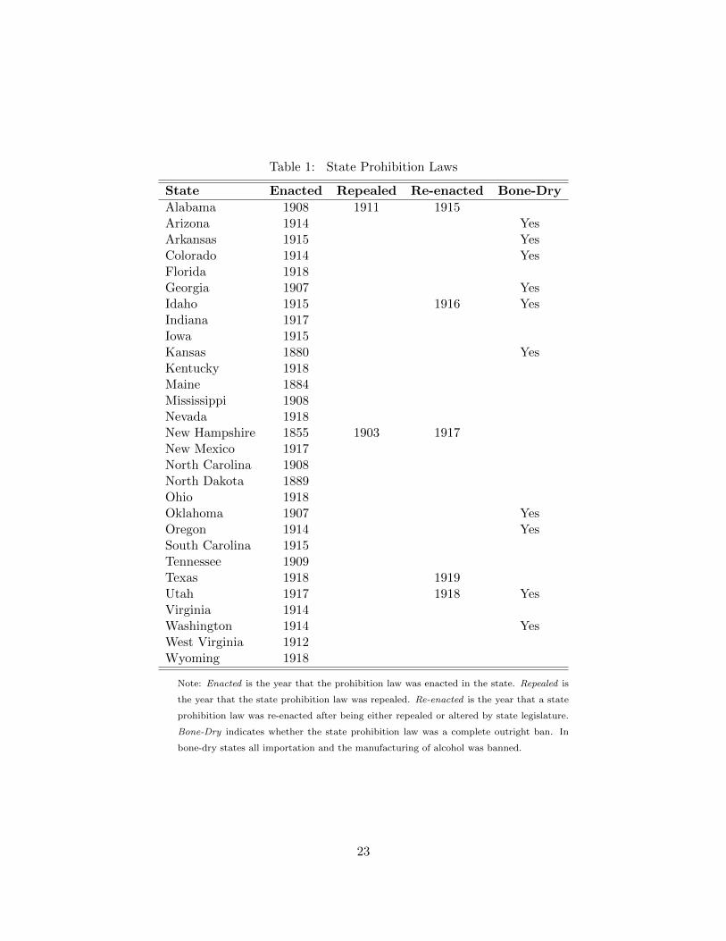
Table 1: State Prohibition Laws

State Enacted Repealed Re-enacted Bone-Dry

Alabama 1908 1911 1915Arizona 1914 YesArkansas 1915 YesColorado 1914 YesFlorida 1918Georgia 1907 YesIdaho 1915 1916 YesIndiana 1917Iowa 1915Kansas 1880 YesKentucky 1918Maine 1884Mississippi 1908Nevada 1918New Hampshire 1855 1903 1917New Mexico 1917North Carolina 1908North Dakota 1889Ohio 1918Oklahoma 1907 YesOregon 1914 YesSouth Carolina 1915Tennessee 1909Texas 1918 1919Utah 1917 1918 YesVirginia 1914Washington 1914 YesWest Virginia 1912Wyoming 1918

Note: Enacted is the year that the prohibition law was enacted in the state. Repealed is

the year that the state prohibition law was repealed. Re-enacted is the year that a state

prohibition law was re-enacted after being either repealed or altered by state legislature.

Bone-Dry indicates whether the state prohibition law was a complete outright ban. In

bone-dry states all importation and the manufacturing of alcohol was banned.

23

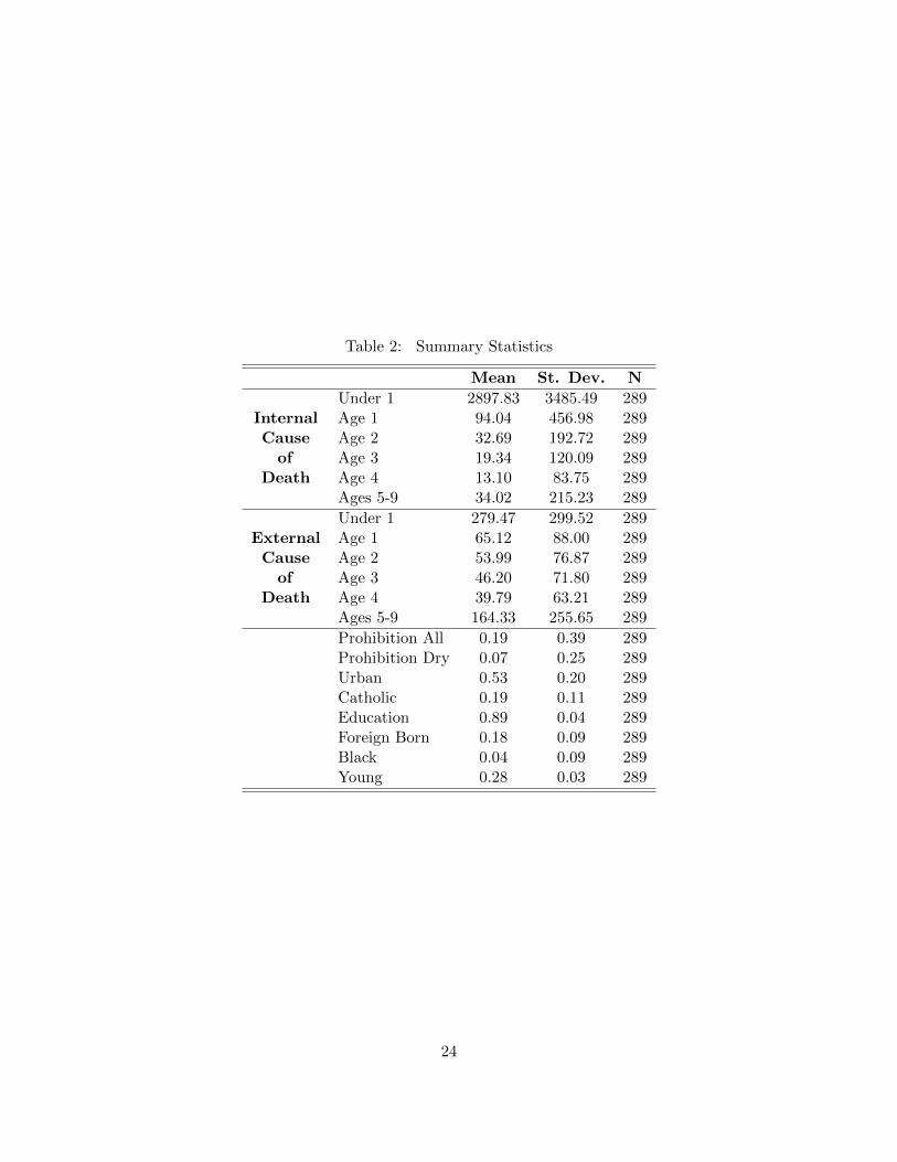
Table 2: Summary Statistics

Mean St. Dev. N

Under 1 2897.83 3485.49 289Internal Age 1 94.04 456.98 289Cause Age 2 32.69 192.72 289of Age 3 19.34 120.09 289

Death Age 4 13.10 83.75 289Ages 5-9 34.02 215.23 289

Under 1 279.47 299.52 289External Age 1 65.12 88.00 289Cause Age 2 53.99 76.87 289of Age 3 46.20 71.80 289

Death Age 4 39.79 63.21 289Ages 5-9 164.33 255.65 289

Prohibition All 0.19 0.39 289Prohibition Dry 0.07 0.25 289Urban 0.53 0.20 289Catholic 0.19 0.11 289Education 0.89 0.04 289Foreign Born 0.18 0.09 289Black 0.04 0.09 289Young 0.28 0.03 289

24

Table 3: Proportion of Internal Deaths: All State Prohibition Laws

Under One Age 1 Age 2 Age 3 Age 4 Ages 5-9(1) (2) (3) (4) (5) (6)

Prohibition All -0.0152 -0.0076 0.0197 0.0125 0.0553* 0.0052(0.0089) (0.0325) (0.0289) (0.0331) (0.0312) (0.0196)

Urban -0.2117 2.1793 0.4034 -1.9402 -1.8846* -1.2393(0.2902) (1.3957) (1.1646) (1.2287) (0.9249) (0.8520)

Catholic 0.0621 0.0895 0.1368 -0.1305 -0.5657 -0.3920(0.1317) (0.7085) (0.6588) (0.7217) (0.8037) (0.6362)

Education -0.3461 1.8664 0.5368 0.9928 0.9702 -0.2409(0.2346) (1.3450) (1.1950) (1.2196) (1.0493) (0.5912)

Foreign Born -0.5043 -1.2771 -1.0995 2.0965 -1.0084 2.0752(0.6008) (3.0148) (2.7886) (2.6461) (2.8404) (2.2604)

Black 1.1808 -12.6905 0.8942 2.4506 15.4268 4.1995(2.8948) (10.8393) (10.3959) (9.3413) (9.1383) (8.3602)

Young 0.1795 7.7410 4.5968 -3.8345 -0.8977 -0.7720(1.2686) (5.9495) (3.6566) (5.1730) (3.4945) (3.4853)

State Fixed Effects Yes Yes Yes Yes Yes YesYear Fixed Effects Yes Yes Yes Yes Yes YesSouth-Year Fixed Effects Yes Yes Yes Yes Yes Yes

R-Square 0.630 0.800 0.732 0.619 0.639 0.785N 289 289 289 289 289 289

a Each column displays a set of regression results. The dependent variable is the proportion of internal causes of death from

internal and external causes. Each regression is weighted by the state population of children under five years of age. Prohibition

All includes all state prohibition laws, both dry laws and non-dry laws.b Standard errors clustered on the state are presented in parentheses.c * 0.10, ** 0.05 and ***0.01 denote significance levels.

25

Table 4: Proportion of Internal Deaths: State Prohibition (Dry Laws Only)


Prohibition Dry -0.0244** 0.0164 0.0558 0.0394 0.1120** -0.0024(0.0108) (0.0494) (0.0463) (0.0585) (0.0514) (0.0287)

Urban -0.0216 3.0438 1.2690 -1.3004 -1.1738 -1.6400(0.3617) (1.9285) (1.5986) (1.4967) (1.3264) (1.2266)

Catholic 0.0441 0.1249 0.2635 0.0481 -0.2854 -0.4043(0.1338) (0.8139) (0.6470) (0.7225) (0.7772) (0.5968)

Education -0.6158** 1.8463 0.3849 0.6375 0.4829 0.1916(0.2448) (1.4453) (1.2550) (1.4545) (1.0206) (0.6109)

Foreign Born -0.9021 -1.6640 -1.2015 1.4402 -0.5066 2.9691(0.6669) (3.4428) (3.1541) (2.9669) (3.0855) (2.4264)

Black 1.2825 -19.4350 -6.1489 2.3257 12.9195 3.2901(3.6352) (13.6285) (15.5331) (14.4742) (13.9201) (12.7320)

Young 1.3728 8.0667 5.3931 -2.5713 0.2812 -2.4128(1.5226) (7.6812) (4.5048) (6.0999) (3.8896) (4.1099)


R-Square 0.616 0.795 0.744 0.614 0.644 0.781N 254 254 254 254 254 254



Dry includes only states that had bone-dry laws.b Standard errors clustered on the state are presented in parentheses.c * 0.10, ** 0.05 and ***0.01 denote significance levels.

26

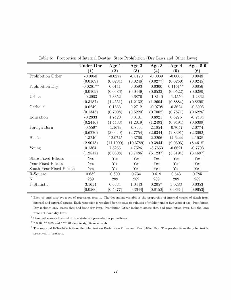
Table 5: Proportion of Internal Deaths: State Prohibition (Dry Laws and Other Laws)


Prohibition Other -0.0050 -0.0277 -0.0170 -0.0039 -0.0003 0.0048(0.0169) (0.0284) (0.0248) (0.0277) (0.0250) (0.0245)

Prohibition Dry -0.0261** 0.0141 0.0593 0.0300 0.1151** 0.0056(0.0109) (0.0486) (0.0449) (0.0523) (0.0522) (0.0280)

Urban -0.2903 2.3352 0.6876 -1.8140 -1.4550 -1.2362(0.3187) (1.4551) (1.2132) (1.2604) (0.8884) (0.8890)

Catholic 0.0249 0.1633 0.2712 -0.0708 -0.3624 -0.3905(0.1343) (0.7008) (0.6220) (0.7002) (0.7871) (0.6226)

Education -0.2833 1.7420 0.3101 0.8921 0.6275 -0.2434(0.2416) (1.4433) (1.2019) (1.2493) (0.9494) (0.6309)

Foreign Born -0.5597 -1.1673 -0.8993 2.1854 -0.7057 2.0774(0.6220) (3.0449) (2.7754) (2.6344) (2.8391) (2.3062)

Black 1.3240 -12.9745 0.3766 2.2206 14.6444 4.1938(2.9013) (11.1000) (10.3789) (9.3944) (9.0303) (8.4618)

Young 0.1364 7.8265 4.7526 -3.7653 -0.6621 -0.7703(1.2517) (6.0808) (3.7486) (5.1237) (3.3194) (3.4697)


R-Square 0.632 0.800 0.734 0.619 0.643 0.785N 289 289 289 289 289 289

F-Statistic 3.1654 0.6334 1.0443 0.2057 3.0283 0.0353[0.0566] [0.5377] [0.3644] [0.8152] [0.0634] [0.9653]



Dry includes only states that had bone-dry laws. Prohibition Other includes states that had prohibition laws, but the laws

were not bone-dry laws.b Standard errors clustered on the state are presented in parentheses.c * 0.10, ** 0.05 and ***0.01 denote significance levels.d The reported F-Statistic is from the joint test on Prohibition Other and Prohibition Dry. The p-value from the joint test is

presented in brackets.

27

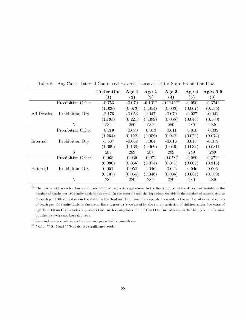
Table 6: Any Cause, Internal Cause, and External Cause of Death: State Prohibition Laws


Prohibition Other -0.753 -0.070 -0.101* -0.114*** -0.090 -0.374*(1.028) (0.073) (0.054) (0.033) (0.062) (0.185)

All Deaths Prohibition Dry -2.176 -0.053 0.047 -0.079 -0.037 -0.042(1.793) (0.221) (0.089) (0.065) (0.046) (0.150)

N 289 289 289 289 289 289

Prohibition Other -0.219 -0.080 -0.013 -0.011 -0.010 -0.032(1.254) (0.122) (0.059) (0.042) (0.026) (0.074)

Internal Prohibition Dry -1.537 -0.062 0.004 -0.013 0.016 -0.019(1.609) (0.168) (0.069) (0.046) (0.032) (0.081)

N 289 289 289 289 289 289

Prohibition Other 0.068 0.039 -0.071 -0.078* -0.089 -0.371*(0.090) (0.056) (0.074) (0.041) (0.063) (0.218)

External Prohibition Dry 0.051 0.052 0.046 -0.042 -0.046 0.006(0.137) (0.054) (0.046) (0.035) (0.034) (0.109)

N 289 289 289 289 289 289

a The results within each column and panel are from separate regressions. In the first (top) panel the dependent variable is the

number of deaths per 1000 individuals in the state. In the second panel the dependent variable is the number of internal causes

of death per 1000 individuals in the state. In the third and final panel the dependent variable is the number of external causes

of death per 1000 individuals in the state. Each regression is weighted by the state population of children under five years of

age. Prohibition Dry includes only states that had bone-dry laws. Prohibition Other includes states that had prohibition laws,

but the laws were not bone-dry laws.b Standard errors clustered on the state are presented in parentheses.c * 0.10, ** 0.05 and ***0.01 denote significance levels.

28

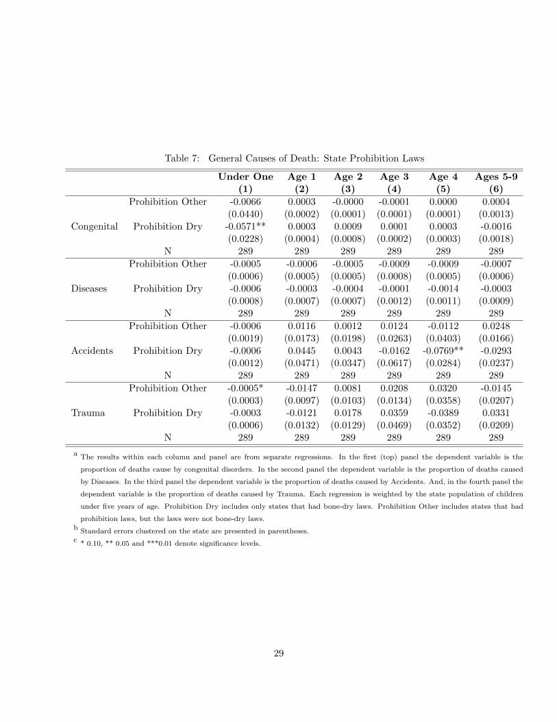
Table 7: General Causes of Death: State Prohibition Laws


Prohibition Other -0.0066 0.0003 -0.0000 -0.0001 0.0000 0.0004(0.0440) (0.0002) (0.0001) (0.0001) (0.0001) (0.0013)

Congenital Prohibition Dry -0.0571** 0.0003 0.0009 0.0001 0.0003 -0.0016(0.0228) (0.0004) (0.0008) (0.0002) (0.0003) (0.0018)

N 289 289 289 289 289 289


Diseases Prohibition Dry -0.0006 -0.0003 -0.0004 -0.0001 -0.0014 -0.0003(0.0008) (0.0007) (0.0007) (0.0012) (0.0011) (0.0009)

N 289 289 289 289 289 289

Prohibition Other -0.0006 0.0116 0.0012 0.0124 -0.0112 0.0248(0.0019) (0.0173) (0.0198) (0.0263) (0.0403) (0.0166)

Accidents Prohibition Dry -0.0006 0.0445 0.0043 -0.0162 -0.0769** -0.0293(0.0012) (0.0471) (0.0347) (0.0617) (0.0284) (0.0237)

N 289 289 289 289 289 289

Prohibition Other -0.0005* -0.0147 0.0081 0.0208 0.0320 -0.0145(0.0003) (0.0097) (0.0103) (0.0134) (0.0358) (0.0207)

Trauma Prohibition Dry -0.0003 -0.0121 0.0178 0.0359 -0.0389 0.0331(0.0006) (0.0132) (0.0129) (0.0469) (0.0352) (0.0209)

N 289 289 289 289 289 289

a The results within each column and panel are from separate regressions. In the first (top) panel the dependent variable is the

proportion of deaths cause by congenital disorders. In the second panel the dependent variable is the proportion of deaths caused

by Diseases. In the third panel the dependent variable is the proportion of deaths caused by Accidents. And, in the fourth panel the

dependent variable is the proportion of deaths caused by Trauma. Each regression is weighted by the state population of children

under five years of age. Prohibition Dry includes only states that had bone-dry laws. Prohibition Other includes states that had

prohibition laws, but the laws were not bone-dry laws.b Standard errors clustered on the state are presented in parentheses.c * 0.10, ** 0.05 and ***0.01 denote significance levels.

29

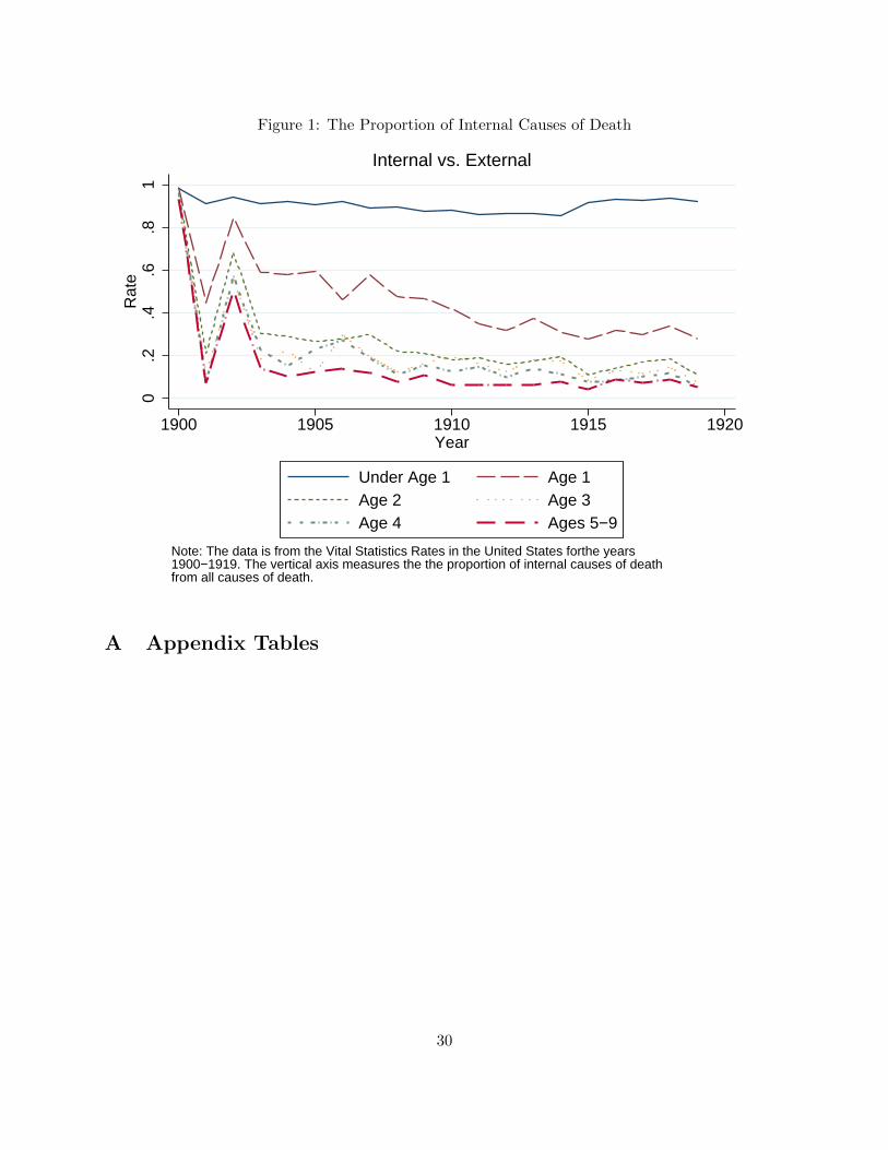
Figure 1: The Proportion of Internal Causes of Death

0.2

.4.6

.81

Rat

e

1900 1905 1910 1915 1920Year

Under Age 1 Age 1Age 2 Age 3Age 4 Ages 5−9

Note: The data is from the Vital Statistics Rates in the United States forthe years1900−1919. The vertical axis measures the the proportion of internal causes of deathfrom all causes of death.

Internal vs. External

A Appendix Tables

30

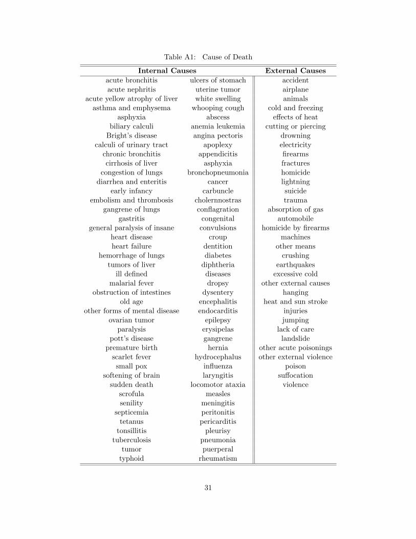
Table A1: Cause of Death

Internal Causes External Causes

acute bronchitis ulcers of stomach accidentacute nephritis uterine tumor airplane

acute yellow atrophy of liver white swelling animalsasthma and emphysema whooping cough cold and freezing

asphyxia abscess effects of heatbiliary calculi anemia leukemia cutting or piercing

Bright’s disease angina pectoris drowningcalculi of urinary tract apoplexy electricity

chronic bronchitis appendicitis firearmscirrhosis of liver asphyxia fractures

congestion of lungs bronchopneumonia homicidediarrhea and enteritis cancer lightning

early infancy carbuncle suicideembolism and thrombosis cholernnostras trauma

gangrene of lungs conflagration absorption of gasgastritis congenital automobile

general paralysis of insane convulsions homicide by firearmsheart disease croup machinesheart failure dentition other means

hemorrhage of lungs diabetes crushingtumors of liver diphtheria earthquakes

ill defined diseases excessive coldmalarial fever dropsy other external causes

obstruction of intestines dysentery hangingold age encephalitis heat and sun stroke

other forms of mental disease endocarditis injuriesovarian tumor epilepsy jumping

paralysis erysipelas lack of carepott’s disease gangrene landslide

premature birth hernia other acute poisoningsscarlet fever hydrocephalus other external violencesmall pox influenza poison

softening of brain laryngitis suffocationsudden death locomotor ataxia violence

scrofula measlessenility meningitis

septicemia peritonitistetanus pericarditis

tonsillitis pleurisytuberculosis pneumonia

tumor puerperaltyphoid rheumatism

31

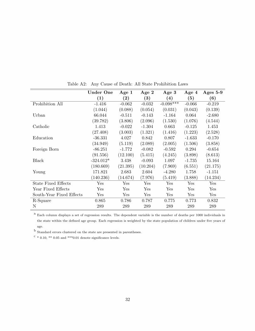
Table A2: Any Cause of Death: All State Prohibition Laws


Prohibition All -1.416 -0.062 -0.032 -0.098*** -0.066 -0.219(1.044) (0.088) (0.054) (0.031) (0.043) (0.139)

Urban 66.044 -0.511 -0.143 -1.164 0.064 -2.680(39.782) (3.806) (2.096) (1.530) (1.076) (4.544)

Catholic 1.413 -0.022 -1.304 0.663 -0.125 1.453(27.408) (3.003) (1.321) (1.416) (1.223) (2.528)

Education -36.331 4.027 0.842 0.807 -1.633 -0.170(34.949) (5.119) (2.089) (2.005) (1.506) (3.858)

Foreign Born -86.251 -1.772 -0.082 -0.592 0.294 -0.654(91.556) (12.100) (5.415) (4.245) (3.898) (8.613)

Black -324.012* 3.438 -0.093 1.097 -1.735 15.164(180.669) (21.395) (10.204) (7.969) (6.551) (21.175)

Young 171.821 2.683 2.604 -4.280 1.758 -1.151(140.236) (14.674) (7.976) (5.419) (3.888) (14.234)


R-Square 0.865 0.786 0.787 0.775 0.773 0.832N 289 289 289 289 289 289

a Each column displays a set of regression results. The dependent variable is the number of deaths per 1000 individuals in

the state within the defined age group. Each regression is weighted by the state population of children under five years of

age.b Standard errors clustered on the state are presented in parentheses.c * 0.10, ** 0.05 and ***0.01 denote significance levels.

32

Table A3: Any Cause of Death: State Prohibition (Dry Laws Only)


Prohibition Dry -1.775 -0.031 0.058 -0.084 -0.037 -0.033(1.851) (0.228) (0.092) (0.067) (0.045) (0.155)

Urban 90.448* 0.637 1.201 -1.072 1.126 0.976(50.749) (4.923) (2.529) (1.999) (1.265) (4.617)

Catholic 0.195 0.107 -0.948 0.810 0.111 2.175(28.416) (3.078) (1.315) (1.423) (1.269) (2.687)

Education -52.795 2.779 -0.826 0.536 -3.156* -3.680(43.496) (5.891) (2.387) (2.443) (1.788) (4.009)

Foreign Born -138.246 -3.112 -0.677 -0.214 0.034 -2.150(105.369) (13.733) (5.967) (4.638) (3.900) (8.936)

Black -388.756 4.972 -1.029 0.781 -3.541 2.206(234.403) (26.499) (11.814) (9.697) (7.372) (24.619)

Young 244.992 5.731 6.227 -3.611 6.305 8.666(183.082) (16.898) (9.136) (6.606) (5.099) (14.335)


R-Square 0.844 0.771 0.777 0.761 0.778 0.829N 254 254 254 254 254 254

a Each column displays a set of regression results. The dependent variable is the number of deaths per 1000 individuals

in the state within the defined age group. Each regression is weighted by the state population of children under five

years of age.b Standard errors clustered on the state are presented in parentheses.c * 0.10, ** 0.05 and ***0.01 denote significance levels.

33

Table A4: Any Cause of Death: State Prohibition (Dry Laws and Other Laws)


Prohibition Other -0.753 -0.070 -0.101* -0.114*** -0.090 -0.374*(1.028) (0.073) (0.054) (0.033) (0.062) (0.185)

Prohibition Dry -2.176 -0.053 0.047 -0.079 -0.037 -0.042(1.793) (0.221) (0.089) (0.065) (0.046) (0.150)

Urban 61.138 -0.450 0.365 -1.041 0.247 -1.534(41.715) (4.051) (2.115) (1.590) (1.037) (4.015)

Catholic -0.970 0.008 -1.057 0.723 -0.037 2.009(26.769) (2.954) (1.272) (1.393) (1.227) (2.506)

Education -32.712 3.982 0.468 0.716 -1.767 -1.016(37.947) (5.651) (2.217) (2.126) (1.502) (3.618)

Foreign Born -91.180 -1.711 0.428 -0.468 0.477 0.497(93.837) (12.717) (5.539) (4.399) (3.992) (8.601)

Black -310.656 3.274 -1.475 0.761 -2.232 12.044(184.935) (22.828) (10.921) (8.229) (6.679) (20.502)

Young 171.257 2.690 2.662 -4.265 1.779 -1.019(137.865) (14.653) (7.911) (5.418) (3.823) (13.065)


R-Square 0.865 0.786 0.788 0.775 0.773 0.834N 289 289 289 289 289 289

F-Statistic 0.9089 0.9157 1.7492 9.3150 1.3646 2.0562[0.4138] [0.4111] [0.1912] [0.0007] [0.2709] [0.1456]

a Each column displays a set of regression results. The dependent variable is the number of deaths per 1000 individuals in

the state within the defined age group. Each regression is weighted by the state population of children under five years of

age.b Standard errors clustered on the state are presented in parentheses.c * 0.10, ** 0.05 and ***0.01 denote significance levels.d The reported F-Statistic is from the joint test on Prohibition Other and Prohibition Dry. The p-value from the joint test

is presented in brackets.

34

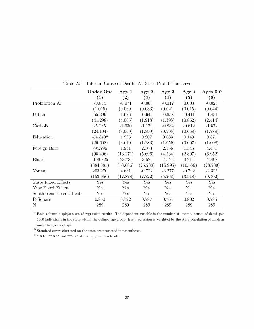
Table A5: Internal Cause of Death: All State Prohibition Laws


Prohibition All -0.854 -0.071 -0.005 -0.012 0.003 -0.026(1.015) (0.069) (0.033) (0.021) (0.015) (0.044)

Urban 55.399 1.626 -0.642 -0.658 -0.411 -1.451(41.298) (4.005) (1.918) (1.395) (0.862) (2.414)

Catholic -5.285 -1.030 -1.170 -0.834 -0.612 -1.572(24.104) (3.069) (1.399) (0.995) (0.658) (1.788)

Education -54.340* 1.926 0.207 0.683 0.149 0.371(29.608) (3.610) (1.283) (1.059) (0.607) (1.608)

Foreign Born -94.796 1.931 2.363 2.156 1.345 4.431(95.406) (13.271) (5.696) (4.234) (2.807) (6.952)

Black -106.325 -23.730 -3.522 -4.126 0.211 -2.498(384.385) (58.686) (25.233) (15.995) (10.556) (28.930)

Young 203.270 4.681 -0.722 -3.277 -0.792 -2.326(153.956) (17.878) (7.722) (5.268) (3.518) (9.402)


R-Square 0.850 0.792 0.787 0.764 0.802 0.785N 289 289 289 289 289 289

a Each column displays a set of regression results. The dependent variable is the number of internal causes of death per

1000 individuals in the state within the defined age group. Each regression is weighted by the state population of children

under five years of age.b Standard errors clustered on the state are presented in parentheses.c * 0.10, ** 0.05 and ***0.01 denote significance levels.

35

Table A6: Internal Cause of Death: State Prohibition (Dry Laws Only)


Prohibition Dry -1.083 -0.042 0.006 -0.011 0.015 -0.019(1.683) (0.152) (0.063) (0.042) (0.030) (0.077)

Urban 67.852 2.448 -0.736 -0.675 -0.269 -1.940(56.432) (6.604) (3.175) (2.226) (1.366) (3.842)

Catholic -7.666 -0.912 -1.123 -0.816 -0.537 -1.556(24.533) (3.067) (1.401) (0.972) (0.650) (1.735)

Education -71.141* 1.337 0.367 0.966 0.121 0.729(39.609) (3.716) (1.253) (1.101) (0.637) (1.583)

Foreign Born -140.624 0.993 2.622 2.255 1.566 5.215(107.738) (15.151) (6.509) (4.834) (3.176) (7.863)

Black -76.415 -22.544 -3.197 -5.100 -0.655 -0.473(579.891) (91.043) (39.866) (25.392) (16.583) (45.749)

Young 260.035 5.830 -1.838 -4.252 -0.927 -4.538(184.408) (19.750) (8.776) (6.023) (3.982) (10.758)


R-Square 0.829 0.785 0.785 0.763 0.802 0.785N 254 254 254 254 254 254




36

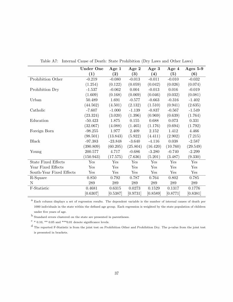
Table A7: Internal Cause of Death: State Prohibition (Dry Laws and Other Laws)



Prohibition Dry -1.537 -0.062 0.004 -0.013 0.016 -0.019(1.609) (0.168) (0.069) (0.046) (0.032) (0.081)

Urban 50.489 1.691 -0.577 -0.663 -0.316 -1.402(44.562) (4.501) (2.132) (1.510) (0.941) (2.635)

Catholic -7.607 -1.000 -1.139 -0.837 -0.567 -1.549(23.324) (3.020) (1.396) (0.969) (0.639) (1.764)

Education -50.423 1.875 0.155 0.688 0.073 0.331(32.067) (4.088) (1.465) (1.176) (0.694) (1.792)

Foreign Born -98.255 1.977 2.409 2.152 1.412 4.466(98.501) (13.843) (5.922) (4.411) (2.902) (7.215)

Black -97.383 -23.848 -3.640 -4.116 0.038 -2.587(390.809) (60.205) (25.804) (16.420) (10.760) (29.549)

Young 200.577 4.717 -0.686 -3.280 -0.740 -2.299(150.943) (17.575) (7.636) (5.201) (3.487) (9.330)


R-Square 0.850 0.792 0.787 0.764 0.802 0.785N 289 289 289 289 289 289

F-Statistic 0.4681 0.6315 0.0273 0.1529 0.1317 0.1776[0.6307] [0.5387] [0.9731] [0.8589] [0.8771] [0.8381]



under five years of age.b Standard errors clustered on the state are presented in parentheses.c * 0.10, ** 0.05 and ***0.01 denote significance levels.d The reported F-Statistic is from the joint test on Prohibition Other and Prohibition Dry. The p-value from the joint test


37

Table A8: External Cause of Death: All State Prohibition Laws


Prohibition All 0.060 0.045 -0.014 -0.061* -0.068 -0.189(0.088) (0.037) (0.053) (0.032) (0.042) (0.157)

Urban 2.683* -1.876** 0.307 -0.627 0.415 -2.114(1.436) (0.743) (1.024) (0.722) (0.926) (3.648)

Catholic 1.066 0.701 -0.206 1.346*** 0.553 3.063***(0.931) (0.477) (0.562) (0.407) (0.730) (1.044)

Education 1.959 1.604 0.383 -0.238 -1.808 -0.751(1.762) (1.111) (1.140) (1.015) (1.224) (3.485)

Foreign Born -7.928*** -3.175* -2.350 -3.095** -1.381 -5.980(2.775) (1.740) (1.469) (1.233) (2.070) (4.838)

Black 32.124*** 21.356*** 3.673 13.397** -2.603 35.375*(11.587) (5.960) (6.237) (6.329) (5.749) (19.035)

Young 8.655* -2.980 2.106 0.764 1.827 1.843(4.501) (3.106) (3.442) (2.243) (3.069) (11.906)


R-Square 0.901 0.841 0.861 0.866 0.818 0.906N 289 289 289 289 289 289

a Each column displays a set of regression results. The dependent variable is the number of external causes of death per



38

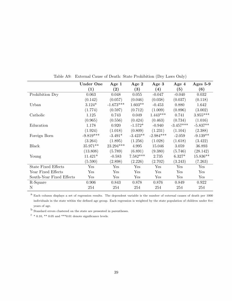
Table A9: External Cause of Death: State Prohibition (Dry Laws Only)


Prohibition Dry 0.063 0.048 0.055 -0.047 -0.040 0.032(0.142) (0.057) (0.046) (0.038) (0.037) (0.118)

Urban 3.124* -1.673*** 1.603** -0.453 0.880 1.642(1.774) (0.597) (0.712) (1.009) (0.896) (3.002)

Catholic 1.125 0.743 0.049 1.443*** 0.741 3.955***(0.965) (0.556) (0.424) (0.463) (0.734) (1.016)

Education 1.178 0.920 -1.572* -0.940 -3.457*** -5.837**(1.924) (1.018) (0.809) (1.231) (1.104) (2.388)

Foreign Born -9.819*** -3.491* -3.423** -2.984*** -2.059 -9.139**(3.264) (1.895) (1.256) (1.028) (1.618) (3.422)

Black 35.971** 23.294*** 4.995 15.046 3.059 36.893(13.808) (5.789) (6.891) (9.380) (5.746) (28.142)

Young 11.421* -0.583 7.582*** 2.735 6.327* 15.836**(5.590) (2.898) (2.226) (2.702) (3.243) (7.263)


R-Square 0.906 0.843 0.878 0.876 0.849 0.922N 254 254 254 254 254 254

a Each column displays a set of regression results. The dependent variable is the number of external causes of death per 1000

individuals in the state within the defined age group. Each regression is weighted by the state population of children under five

years of age.b Standard errors clustered on the state are presented in parentheses.c * 0.10, ** 0.05 and ***0.01 denote significance levels.

39

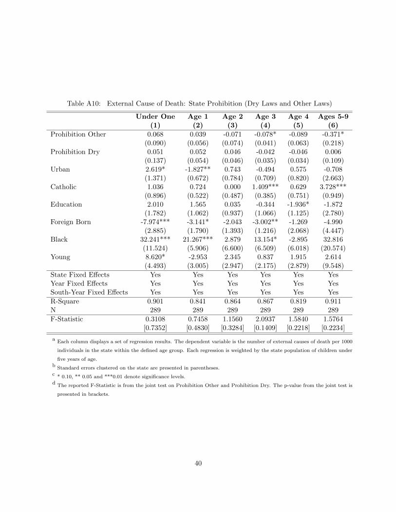
Table A10: External Cause of Death: State Prohibition (Dry Laws and Other Laws)


Prohibition Other 0.068 0.039 -0.071 -0.078* -0.089 -0.371*(0.090) (0.056) (0.074) (0.041) (0.063) (0.218)

Prohibition Dry 0.051 0.052 0.046 -0.042 -0.046 0.006(0.137) (0.054) (0.046) (0.035) (0.034) (0.109)

Urban 2.619* -1.827** 0.743 -0.494 0.575 -0.708(1.371) (0.672) (0.784) (0.709) (0.820) (2.663)

Catholic 1.036 0.724 0.000 1.409*** 0.629 3.728***(0.896) (0.522) (0.487) (0.385) (0.751) (0.949)

Education 2.010 1.565 0.035 -0.344 -1.936* -1.872(1.782) (1.062) (0.937) (1.066) (1.125) (2.780)

Foreign Born -7.974*** -3.141* -2.043 -3.002** -1.269 -4.990(2.885) (1.790) (1.393) (1.216) (2.068) (4.447)

Black 32.241*** 21.267*** 2.879 13.154* -2.895 32.816(11.524) (5.906) (6.600) (6.509) (6.018) (20.574)

Young 8.620* -2.953 2.345 0.837 1.915 2.614(4.493) (3.005) (2.947) (2.175) (2.879) (9.548)


R-Square 0.901 0.841 0.864 0.867 0.819 0.911N 289 289 289 289 289 289

F-Statistic 0.3108 0.7458 1.1560 2.0937 1.5840 1.5764[0.7352] [0.4830] [0.3284] [0.1409] [0.2218] [0.2234]

a Each column displays a set of regression results. The dependent variable is the number of external causes of death per 1000

individuals in the state within the defined age group. Each regression is weighted by the state population of children under

five years of age.b Standard errors clustered on the state are presented in parentheses.c * 0.10, ** 0.05 and ***0.01 denote significance levels.d The reported F-Statistic is from the joint test on Prohibition Other and Prohibition Dry. The p-value from the joint test is


40

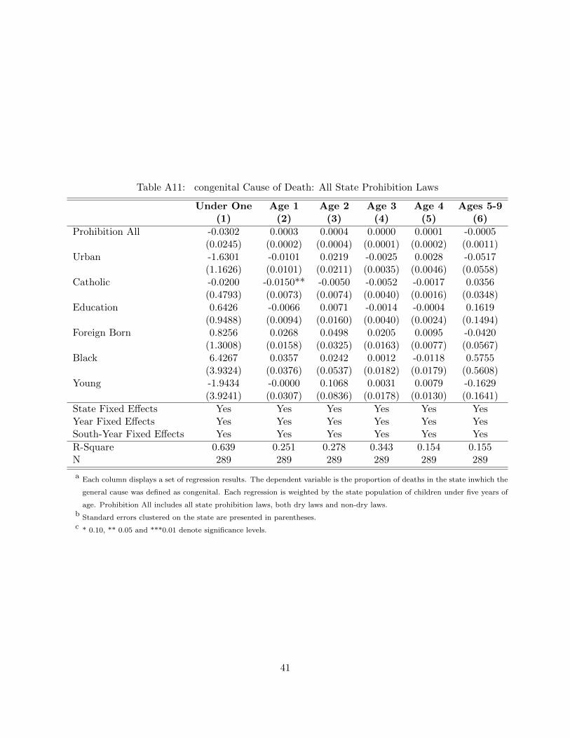
Table A11: congenital Cause of Death: All State Prohibition Laws


Prohibition All -0.0302 0.0003 0.0004 0.0000 0.0001 -0.0005(0.0245) (0.0002) (0.0004) (0.0001) (0.0002) (0.0011)

Urban -1.6301 -0.0101 0.0219 -0.0025 0.0028 -0.0517(1.1626) (0.0101) (0.0211) (0.0035) (0.0046) (0.0558)

Catholic -0.0200 -0.0150** -0.0050 -0.0052 -0.0017 0.0356(0.4793) (0.0073) (0.0074) (0.0040) (0.0016) (0.0348)

Education 0.6426 -0.0066 0.0071 -0.0014 -0.0004 0.1619(0.9488) (0.0094) (0.0160) (0.0040) (0.0024) (0.1494)

Foreign Born 0.8256 0.0268 0.0498 0.0205 0.0095 -0.0420(1.3008) (0.0158) (0.0325) (0.0163) (0.0077) (0.0567)

Black 6.4267 0.0357 0.0242 0.0012 -0.0118 0.5755(3.9324) (0.0376) (0.0537) (0.0182) (0.0179) (0.5608)

Young -1.9434 -0.0000 0.1068 0.0031 0.0079 -0.1629(3.9241) (0.0307) (0.0836) (0.0178) (0.0130) (0.1641)


R-Square 0.639 0.251 0.278 0.343 0.154 0.155N 289 289 289 289 289 289

a Each column displays a set of regression results. The dependent variable is the proportion of deaths in the state inwhich the

general cause was defined as congenital. Each regression is weighted by the state population of children under five years of

age. Prohibition All includes all state prohibition laws, both dry laws and non-dry laws.b Standard errors clustered on the state are presented in parentheses.c * 0.10, ** 0.05 and ***0.01 denote significance levels.

41

Table A12: congenital Cause of Death: State Prohibition (Dry Laws Only)


Prohibition Dry -0.0553** 0.0003 0.0009 0.0001 0.0003 -0.0018(0.0228) (0.0004) (0.0008) (0.0002) (0.0003) (0.0020)

Urban -0.8988 -0.0164 0.0252 -0.0034 0.0029 -0.0939(1.0802) (0.0118) (0.0269) (0.0045) (0.0052) (0.0841)

Catholic -0.0528 -0.0157** -0.0035 -0.0050 -0.0015 0.0308(0.4524) (0.0074) (0.0084) (0.0037) (0.0016) (0.0284)

Education 0.0768 -0.0054 0.0041 -0.0014 -0.0003 0.1982(0.9312) (0.0115) (0.0210) (0.0048) (0.0031) (0.1725)

Foreign Born -0.2602 0.0308* 0.0536 0.0237 0.0109 -0.0212(1.3417) (0.0172) (0.0337) (0.0179) (0.0089) (0.0622)

Black 4.4213 0.0552 0.0081 0.0020 -0.0188 0.6989(3.7805) (0.0465) (0.0620) (0.0219) (0.0253) (0.6427)

Young 1.2219 -0.0138 0.1123 -0.0011 0.0051 -0.2862(3.8801) (0.0335) (0.0984) (0.0218) (0.0127) (0.2400)


R-Square 0.665 0.259 0.283 0.345 0.159 0.167N 254 254 254 254 254 254


general cause was defined as congenital. Each regression is weighted by the state population of children under five years of

age. Prohibition Dry includes only states that had bone-dry laws.b Standard errors clustered on the state are presented in parentheses.c * 0.10, ** 0.05 and ***0.01 denote significance levels.

42

Table A13: congenital Cause of Death: State Prohibition (Dry Laws and Other Laws)


Prohibition Other -0.0066 0.0003 -0.0000 -0.0001 0.0000 0.0004(0.0440) (0.0002) (0.0001) (0.0001) (0.0001) (0.0013)

Prohibition Dry -0.0571** 0.0003 0.0009 0.0001 0.0003 -0.0016(0.0228) (0.0004) (0.0008) (0.0002) (0.0003) (0.0018)

Urban -1.8042 -0.0100 0.0251 -0.0017 0.0037 -0.0588(1.1705) (0.0111) (0.0227) (0.0036) (0.0053) (0.0612)

Catholic -0.1045 -0.0149** -0.0035 -0.0049 -0.0012 0.0321(0.4928) (0.0071) (0.0079) (0.0037) (0.0014) (0.0320)

Education 0.7710 -0.0067 0.0047 -0.0020 -0.0010 0.1671(0.9710) (0.0096) (0.0175) (0.0043) (0.0027) (0.1532)

Foreign Born 0.6507 0.0269 0.0530 0.0212 0.0103 -0.0491(1.4435) (0.0168) (0.0345) (0.0169) (0.0085) (0.0599)

Black 6.9006* 0.0354 0.0155 -0.0009 -0.0141 0.5949(3.9146) (0.0401) (0.0557) (0.0186) (0.0200) (0.5790)

Young -1.9634 -0.0000 0.1071 0.0032 0.0080 -0.1637(4.1090) (0.0308) (0.0823) (0.0179) (0.0131) (0.1651)


R-Square 0.642 0.251 0.280 0.343 0.155 0.157N 289 289 289 289 289 289

F-Statistic 3.3341 1.5573 0.7596 0.5487 0.4707 0.4494[0.0493] [0.2273] [0.4766] [0.5834] [0.6291] [0.6422]

a Each column displays a set of regression results. The dependent variable is the proportion of the number of deaths in the

state that the general cause was defined as congenital. Each regression is weighted by the state population of children under

five years of age. Prohibition Dry includes only states that had bone-dry laws. Prohibition Other includes states that had

prohibition laws, but the laws were not bone-dry laws.b Standard errors clustered on the state are presented in parentheses.c * 0.10, ** 0.05 and ***0.01 denote significance levels.d The reported F-Statistic is from the joint test on Prohibition Other and Prohibition Dry. The p-value from the joint test is


43

Table A14: diseases Cause of Death: All State Prohibition Laws


Prohibition All -0.0006 -0.0004 -0.0005 -0.0005 -0.0011* -0.0005(0.0005) (0.0005) (0.0005) (0.0008) (0.0006) (0.0006)

Urban -0.0269 -0.0231 -0.0252 -0.0589 0.0075 -0.0287(0.0265) (0.0226) (0.0232) (0.0569) (0.0256) (0.0295)

Catholic -0.0203 -0.0185 -0.0220 -0.0307 -0.0046 -0.0206(0.0188) (0.0167) (0.0177) (0.0293) (0.0209) (0.0196)

Education 0.0019 -0.0037 -0.0001 -0.0172 0.0292 -0.0038(0.0164) (0.0157) (0.0154) (0.0269) (0.0255) (0.0179)

Foreign Born 0.0695 0.0771 0.0726 0.1675 0.0224 0.0958(0.0696) (0.0653) (0.0662) (0.1357) (0.0785) (0.0804)

Black 0.0619 0.0418 0.0598 0.0810 0.0703 0.0533(0.1186) (0.1010) (0.1056) (0.1352) (0.1301) (0.1163)

Young 0.0227 0.0148 0.0102 -0.0230 0.1862 0.0260(0.1076) (0.0924) (0.0979) (0.1817) (0.1173) (0.1142)


R-Square 0.702 0.661 0.660 0.649 0.500 0.703N 289 289 289 289 289 289

a Each column displays a set of regression results. The dependent variable is the proportion of deaths in the state inwhich

the general cause was defined as diseases. Each regression is weighted by the state population of children under five years

of age. Prohibition All includes all state prohibition laws, both dry laws and non-dry laws.b Standard errors clustered on the state are presented in parentheses.c * 0.10, ** 0.05 and ***0.01 denote significance levels.

44

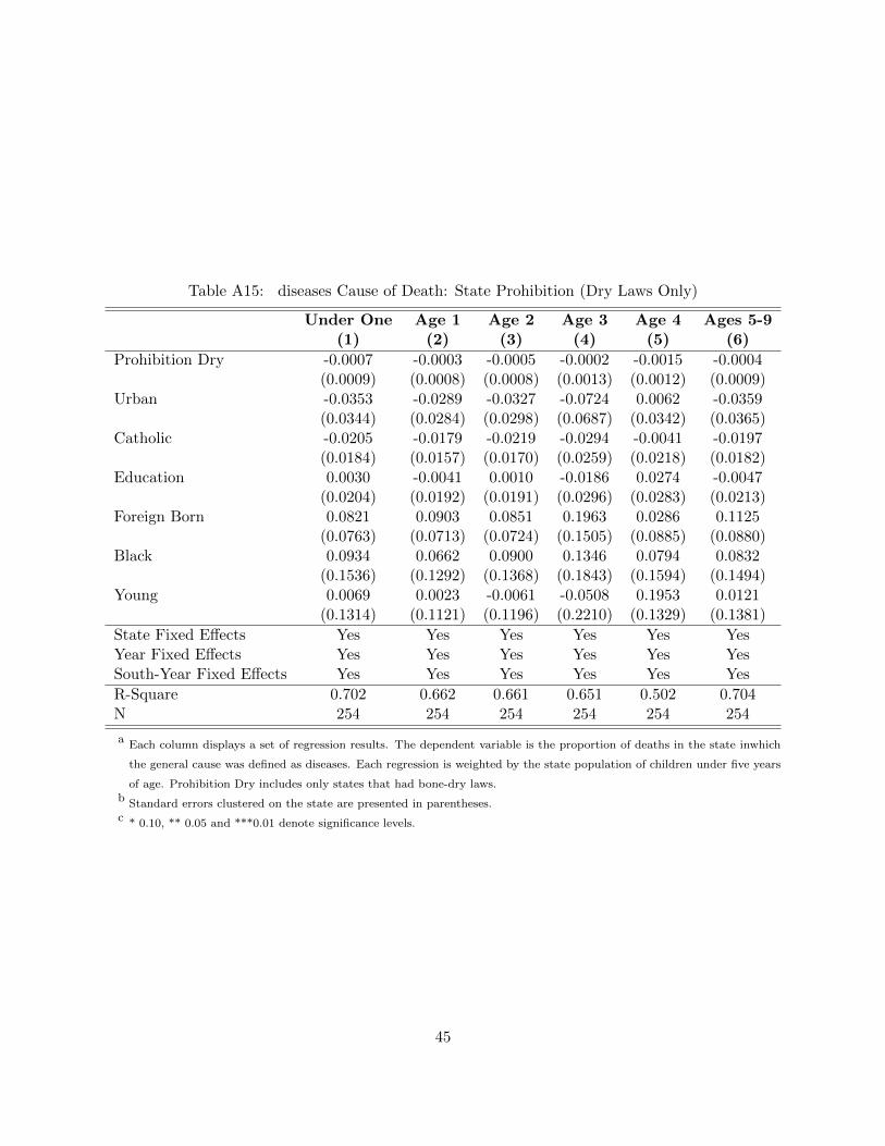
Table A15: diseases Cause of Death: State Prohibition (Dry Laws Only)


Prohibition Dry -0.0007 -0.0003 -0.0005 -0.0002 -0.0015 -0.0004(0.0009) (0.0008) (0.0008) (0.0013) (0.0012) (0.0009)

Urban -0.0353 -0.0289 -0.0327 -0.0724 0.0062 -0.0359(0.0344) (0.0284) (0.0298) (0.0687) (0.0342) (0.0365)

Catholic -0.0205 -0.0179 -0.0219 -0.0294 -0.0041 -0.0197(0.0184) (0.0157) (0.0170) (0.0259) (0.0218) (0.0182)

Education 0.0030 -0.0041 0.0010 -0.0186 0.0274 -0.0047(0.0204) (0.0192) (0.0191) (0.0296) (0.0283) (0.0213)

Foreign Born 0.0821 0.0903 0.0851 0.1963 0.0286 0.1125(0.0763) (0.0713) (0.0724) (0.1505) (0.0885) (0.0880)

Black 0.0934 0.0662 0.0900 0.1346 0.0794 0.0832(0.1536) (0.1292) (0.1368) (0.1843) (0.1594) (0.1494)

Young 0.0069 0.0023 -0.0061 -0.0508 0.1953 0.0121(0.1314) (0.1121) (0.1196) (0.2210) (0.1329) (0.1381)


R-Square 0.702 0.662 0.661 0.651 0.502 0.704N 254 254 254 254 254 254


the general cause was defined as diseases. Each regression is weighted by the state population of children under five years

of age. Prohibition Dry includes only states that had bone-dry laws.b Standard errors clustered on the state are presented in parentheses.c * 0.10, ** 0.05 and ***0.01 denote significance levels.

45

Table A16: diseases Cause of Death: State Prohibition (Dry Laws and Other Laws)



Prohibition Dry -0.0006 -0.0003 -0.0004 -0.0001 -0.0014 -0.0003(0.0008) (0.0007) (0.0007) (0.0012) (0.0011) (0.0009)

Urban -0.0273 -0.0220 -0.0250 -0.0560 0.0057 -0.0274(0.0278) (0.0230) (0.0241) (0.0552) (0.0281) (0.0296)

Catholic -0.0205 -0.0180 -0.0219 -0.0293 -0.0055 -0.0199(0.0189) (0.0164) (0.0176) (0.0276) (0.0212) (0.0192)

Education 0.0022 -0.0044 -0.0002 -0.0193 0.0305 -0.0048(0.0177) (0.0169) (0.0165) (0.0288) (0.0272) (0.0191)

Foreign Born 0.0691 0.0781 0.0727 0.1704 0.0206 0.0971(0.0707) (0.0664) (0.0676) (0.1383) (0.0790) (0.0815)

Black 0.0630 0.0390 0.0595 0.0731 0.0752 0.0498(0.1206) (0.1021) (0.1069) (0.1314) (0.1353) (0.1168)

Young 0.0227 0.0149 0.0102 -0.0227 0.1860 0.0262(0.1078) (0.0925) (0.0981) (0.1818) (0.1179) (0.1143)


R-Square 0.702 0.661 0.660 0.649 0.500 0.703N 289 289 289 289 289 289

F-Statistic 0.6538 0.7060 0.5844 0.7336 1.8499 0.8242[0.5273] [0.5016] [0.5636] [0.4886] [0.1747] [0.4483]


state that the general cause was defined as diseases. Each regression is weighted by the state population of children under


prohibition laws, but the laws were not bone-dry laws.b Standard errors clustered on the state are presented in parentheses.c * 0.10, ** 0.05 and ***0.01 denote significance levels.d The reported F-Statistic is from the joint test on Prohibition Other and Prohibition Dry. The p-value from the joint test


46

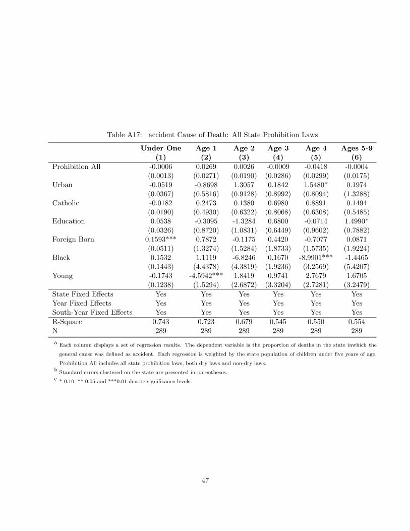
Table A17: accident Cause of Death: All State Prohibition Laws


Prohibition All -0.0006 0.0269 0.0026 -0.0009 -0.0418 -0.0004(0.0013) (0.0271) (0.0190) (0.0286) (0.0299) (0.0175)

Urban -0.0519 -0.8698 1.3057 0.1842 1.5480* 0.1974(0.0367) (0.5816) (0.9128) (0.8992) (0.8094) (1.3288)

Catholic -0.0182 0.2473 0.1380 0.6980 0.8891 0.1494(0.0190) (0.4930) (0.6322) (0.8068) (0.6308) (0.5485)

Education 0.0538 -0.3095 -1.3284 0.6800 -0.0714 1.4990*(0.0326) (0.8720) (1.0831) (0.6449) (0.9602) (0.7882)

Foreign Born 0.1593*** 0.7872 -0.1175 0.4420 -0.7077 0.0871(0.0511) (1.3274) (1.5284) (1.8733) (1.5735) (1.9224)

Black 0.1532 1.1119 -6.8246 0.1670 -8.9901*** -1.4465(0.1443) (4.4378) (4.3819) (1.9236) (3.2569) (5.4207)

Young -0.1743 -4.5942*** 1.8419 0.9741 2.7679 1.6705(0.1238) (1.5294) (2.6872) (3.3204) (2.7281) (3.2479)


R-Square 0.743 0.723 0.679 0.545 0.550 0.554N 289 289 289 289 289 289


general cause was defined as accident. Each regression is weighted by the state population of children under five years of age.

Prohibition All includes all state prohibition laws, both dry laws and non-dry laws.b Standard errors clustered on the state are presented in parentheses.c * 0.10, ** 0.05 and ***0.01 denote significance levels.

47

Table A18: accident Cause of Death: State Prohibition (Dry Laws Only)


Prohibition Dry -0.0007 0.0390 -0.0006 -0.0169 -0.0760** -0.0211(0.0012) (0.0453) (0.0352) (0.0620) (0.0307) (0.0241)

Urban -0.0280 -0.9995 1.0700 0.7765 1.8894 1.0682(0.0264) (0.6021) (1.1820) (0.8484) (1.1464) (1.0103)

Catholic -0.0157 0.2720 0.1338 0.6715 0.7871 0.1834(0.0184) (0.4867) (0.6829) (0.8301) (0.6012) (0.4820)

Education 0.0341 -0.3608 -1.4503 0.4739 -0.1052 1.4753*(0.0303) (0.9854) (1.2670) (0.7096) (0.9986) (0.8212)

Foreign Born 0.1395** 1.2363 0.1364 -0.2123 -1.7961 -1.0011(0.0529) (1.4309) (1.7882) (2.0549) (1.8268) (1.7254)

Black 0.0455 1.0378 -6.4232 -0.9076 -10.6808** -2.4594(0.1317) (5.0768) (5.7148) (2.1551) (4.0436) (5.8908)

Young -0.0711 -4.6825** 1.8657 2.8842 4.4194 3.5207(0.0888) (1.8456) (3.7468) (3.4846) (3.9226) (3.1021)


R-Square 0.741 0.731 0.675 0.600 0.549 0.565N 254 254 254 254 254 254


general cause was defined as accident. Each regression is weighted by the state population of children under five years of age.

Prohibition Dry includes only states that had bone-dry laws.b Standard errors clustered on the state are presented in parentheses.c * 0.10, ** 0.05 and ***0.01 denote significance levels.

48

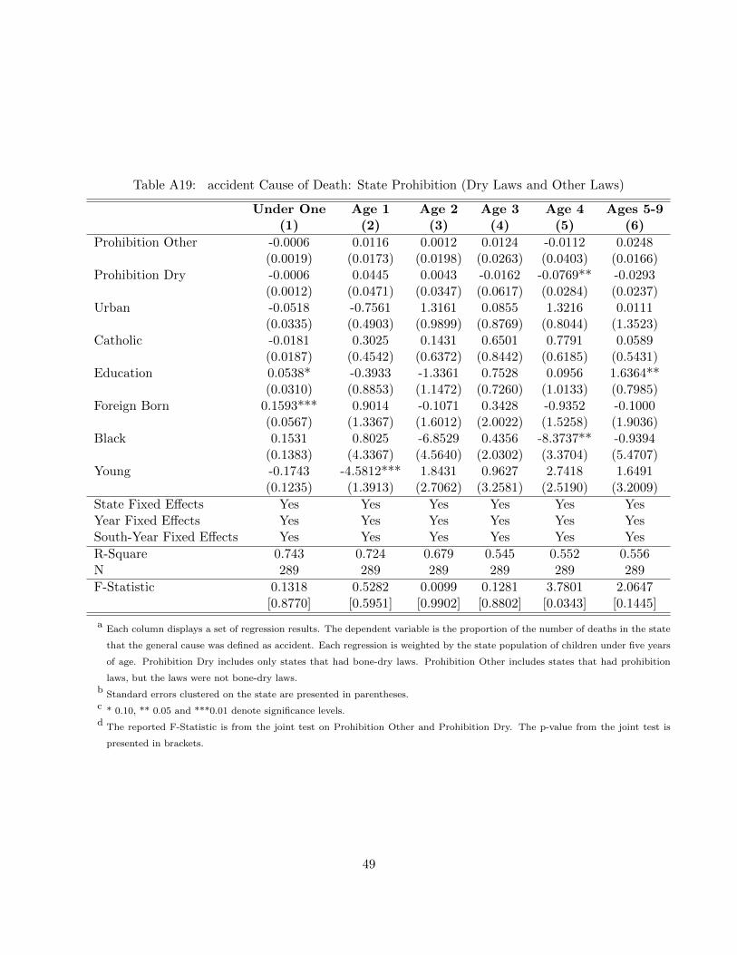
Table A19: accident Cause of Death: State Prohibition (Dry Laws and Other Laws)


Prohibition Other -0.0006 0.0116 0.0012 0.0124 -0.0112 0.0248(0.0019) (0.0173) (0.0198) (0.0263) (0.0403) (0.0166)

Prohibition Dry -0.0006 0.0445 0.0043 -0.0162 -0.0769** -0.0293(0.0012) (0.0471) (0.0347) (0.0617) (0.0284) (0.0237)

Urban -0.0518 -0.7561 1.3161 0.0855 1.3216 0.0111(0.0335) (0.4903) (0.9899) (0.8769) (0.8044) (1.3523)

Catholic -0.0181 0.3025 0.1431 0.6501 0.7791 0.0589(0.0187) (0.4542) (0.6372) (0.8442) (0.6185) (0.5431)

Education 0.0538* -0.3933 -1.3361 0.7528 0.0956 1.6364**(0.0310) (0.8853) (1.1472) (0.7260) (1.0133) (0.7985)

Foreign Born 0.1593*** 0.9014 -0.1071 0.3428 -0.9352 -0.1000(0.0567) (1.3367) (1.6012) (2.0022) (1.5258) (1.9036)

Black 0.1531 0.8025 -6.8529 0.4356 -8.3737** -0.9394(0.1383) (4.3367) (4.5640) (2.0302) (3.3704) (5.4707)

Young -0.1743 -4.5812*** 1.8431 0.9627 2.7418 1.6491(0.1235) (1.3913) (2.7062) (3.2581) (2.5190) (3.2009)


R-Square 0.743 0.724 0.679 0.545 0.552 0.556N 289 289 289 289 289 289

F-Statistic 0.1318 0.5282 0.0099 0.1281 3.7801 2.0647[0.8770] [0.5951] [0.9902] [0.8802] [0.0343] [0.1445]

a Each column displays a set of regression results. The dependent variable is the proportion of the number of deaths in the state

that the general cause was defined as accident. Each regression is weighted by the state population of children under five years

of age. Prohibition Dry includes only states that had bone-dry laws. Prohibition Other includes states that had prohibition

laws, but the laws were not bone-dry laws.b Standard errors clustered on the state are presented in parentheses.c * 0.10, ** 0.05 and ***0.01 denote significance levels.d The reported F-Statistic is from the joint test on Prohibition Other and Prohibition Dry. The p-value from the joint test is


49

Table A20: trauma Cause of Death: All State Prohibition Laws


Prohibition All -0.0004 -0.0135 0.0126 0.0278 -0.0011 0.0077(0.0003) (0.0080) (0.0078) (0.0232) (0.0255) (0.0197)

Urban 0.0096 -0.6229* -0.5116 -0.8648* -0.5049 0.0356(0.0122) (0.3470) (0.3858) (0.4903) (0.9111) (0.5120)

Catholic -0.0040 0.0098 -0.3523 -0.3785 -0.1787 -0.4793(0.0086) (0.1579) (0.3293) (0.4344) (0.6138) (0.3014)

Education -0.0100 0.9848** 0.0630 -0.0800 -1.2986 -0.6174(0.0157) (0.4562) (0.4780) (0.5924) (2.2881) (0.7059)

Foreign Born 0.0051 0.4080 0.5738 1.0372 1.8579 1.4380(0.0174) (0.6663) (1.0639) (1.0053) (1.5210) (0.9669)

Black -0.0400 2.4897 0.8307 1.0107 -1.6040 -0.6606(0.0499) (1.9441) (1.7232) (2.5717) (8.2427) (2.3037)

Young 0.0016 -2.3751** -0.1976 -2.5305 -4.3679 -2.2201(0.0398) (0.9334) (1.1976) (1.5703) (2.8871) (1.3242)


R-Square 0.660 0.597 0.627 0.559 0.566 0.798N 289 289 289 289 289 289


the general cause was defined as trauma. Each regression is weighted by the state population of children under five years of

age. Prohibition All includes all state prohibition laws, both dry laws and non-dry laws.b Standard errors clustered on the state are presented in parentheses.c * 0.10, ** 0.05 and ***0.01 denote significance levels.

50

Table A21: trauma Cause of Death: State Prohibition (Dry Laws Only)


Prohibition Dry -0.0004 -0.0126 0.0140 0.0331 -0.0372 0.0337(0.0006) (0.0138) (0.0131) (0.0469) (0.0347) (0.0212)

Urban 0.0050 -0.6918 -0.8502* -0.9594 -1.2346 -0.2003(0.0129) (0.4703) (0.4169) (0.6643) (1.2997) (0.4847)

Catholic -0.0049 0.0347 -0.3370 -0.3701 -0.3419 -0.4456(0.0093) (0.1619) (0.3251) (0.4626) (0.6042) (0.3026)

Education -0.0064 0.8769 0.2009 -0.1671 -1.0733 -0.7508(0.0172) (0.5629) (0.5856) (0.7573) (2.5958) (0.7118)

Foreign Born 0.0085 0.6078 1.1351 1.2873 2.0131 1.8695*(0.0202) (0.6559) (1.0248) (1.1750) (1.5408) (1.0271)

Black -0.0395 3.1739 2.3851 1.6594 1.9407 0.3103(0.0565) (2.3571) (1.8932) (3.1506) (8.8647) (2.4050)

Young -0.0166 -2.2511 -1.0467 -2.6654 -5.7444 -2.9729**(0.0412) (1.4044) (1.2552) (2.1640) (4.1326) (1.3694)


R-Square 0.670 0.590 0.659 0.549 0.575 0.810N 254 254 254 254 254 254


the general cause was defined as trauma. Each regression is weighted by the state population of children under five years

of age. Prohibition Dry includes only states that had bone-dry laws.b Standard errors clustered on the state are presented in parentheses.c * 0.10, ** 0.05 and ***0.01 denote significance levels.

51

Table A22: trauma Cause of Death: State Prohibition (Dry Laws and Other Laws)


Prohibition Other -0.0005* -0.0147 0.0081 0.0208 0.0320 -0.0145(0.0003) (0.0097) (0.0103) (0.0134) (0.0358) (0.0207)

Prohibition Dry -0.0003 -0.0121 0.0178 0.0359 -0.0389 0.0331(0.0006) (0.0132) (0.0129) (0.0469) (0.0352) (0.0209)

Urban 0.0102 -0.6137 -0.4783 -0.8126* -0.7493 0.2000(0.0128) (0.3647) (0.3904) (0.4712) (0.9403) (0.4800)

Catholic -0.0037 0.0142 -0.3361 -0.3532 -0.2973 -0.3994(0.0090) (0.1595) (0.3347) (0.4510) (0.6125) (0.3077)

Education -0.0104 0.9780** 0.0384 -0.1184 -1.1183 -0.7387(0.0168) (0.4675) (0.5063) (0.6045) (2.2812) (0.7088)

Foreign Born 0.0057 0.4172 0.6073 1.0895 1.6123 1.6032(0.0183) (0.6678) (1.0838) (1.0602) (1.5132) (0.9760)

Black -0.0417 2.4647 0.7400 0.8688 -0.9385 -1.1082(0.0528) (1.9767) (1.7939) (2.5485) (8.0974) (2.3730)

Young 0.0016 -2.3741** -0.1937 -2.5245 -4.3960 -2.2012*(0.0397) (0.9416) (1.2067) (1.5613) (2.8853) (1.2679)


R-Square 0.660 0.597 0.627 0.559 0.568 0.799N 289 289 289 289 289 289

F-Statistic 1.9487 1.6021 1.2442 1.5085 1.2406 1.5276[0.1601] [0.2182] [0.3026] [0.2376] [0.3036] [0.2335]


state that the general cause was defined as trauma. Each regression is weighted by the state population of children under


prohibition laws, but the laws were not bone-dry laws.b Standard errors clustered on the state are presented in parentheses.c * 0.10, ** 0.05 and ***0.01 denote significance levels.d The reported F-Statistic is from the joint test on Prohibition Other and Prohibition Dry. The p-value from the joint test is


52

Documents

Alcohol Prohibition and Infant Mortality1 Alcohol Prohibition and Infant Mortality Briggs Depew Louisiana State University [email protected] Griffin Edwards University of Alabama at Birmingham