Alfred Galichon (NYU Econ+Math) Based on joint works with

VECTOR QUANTILE REGRESSION

Alfred Galichon (NYU Econ+Math)

Based on joint works with G. Carlier and V. Chernozhukov.

November 2017

CARLIER, CHERNOZHUKOV, GALICHON VECTOR QUANTILE REGRESSION SLIDE 1/ 27

REFERENCES

I Carlier, Chernozhukov and G. (2016). “Vector quantile regression: anoptimal transport approach.” Annals of Statistics.

I Carlier, Chernozhukov and G. (2017). “Vector quantile regressionbeyond the specified case.” Journal of multivariate analysis.


Section 1

INTRODUCTION


MOTIVATION: MATZKIN’S IDENTIFICATION OF HEDONIC MODELS

I Consider a standard hedonic model (Ekeland, Heckman and Nesheim,Heckman, Nesheim and Matzkin). A consumer of observedcharacteristics x ∈ Rk and latent characteristics u ∈ R choosing agood whose quality is a scalar y ∈ R (say, the size of a house). Assumeutility of consumer choosing y is given by

S (x , y) + uy

where S (x , y) is the observed part of the consumer surplus, which isassumed to be concave in y , and uy is a preference shock.

I The indirect utility is given by

ϕ (x , u) = maxy{S (x , y) + uy}

so by first order conditions, ∂S (x , y) /∂y + u = 0, thus, lettingψ (x , y) = −S (x , y), quality y is chosen by consumer (x , u (x , y)) suchthat

u (x , y) :=∂ψ (x , y)

∂y

which is nondecreasing in y .


MOTIVATION: MATZKIN’S IDENTIFICATION OF HEDONIC MODELS

I The econometrician:

I assumes U is independent from X and postulates the distribution of U(say, U ([0, 1]))

I observes the distribution of choices Y given observable characteristicsX = x .

I Then (Matzkin), by monotonicity of y (x , u) in u, one has

∂ψ (x , y)

∂y= FY |X (y |x)

which identifies ∂yψ, and hence the marginal surplus surplus ∂yS (x , y).

I By the same token,

∂ϕ (x , u)

∂u= F−1

Y |X (u|x)

identifies ∂uϕ (x , u) to F−1Y |X .


THIS TALK

I The aim of this talk is to:

I generalize this strategy to vector yI obtain a meaningful notion of conditional vector quantileI extend Koenker and Bassett’s (1978) quantile regression to the vector

case


Section 2

CONDITIONAL VECTOR QUANTILES


MULTIVARIATE EXTENSION OF MATZKIN’S STRATEGY

I Now assume quality is a vector y ∈ Rd , and latent characteristics isu ∈ Rd (say, size+amenities). Assume utility of consumer choosing y isgiven by

S (x , y) + u>y

where S (x , y) is still assumed to be concave in y .I As before, let ψ (x , y) = −S (x , y). By first order conditions, quality y

is chosen by consumer (x , u (x , y)) such that

u (x , y) := ∇yψ (x , y)

which, conditional on x , is “vector nondecreasing” in y in a generalizedsense, where vector nondecreasing=gradient of a convex function.

I As before, assume:

I The distribution of U given X = x is µ (say U([0, 1]d

))

I The distribution FY |X of Y given X is observed.

I Question: Is ∇yψ identified as in the scalar case? equivalently, andomitting the dependence in x , is there a convex function ψ (y) such that

∇ψ (Y ) ∼ µ?


IDENTIFICATION VIA MASS TRANSPORTATION

I The answer, is yes. In fact, ψ is the solution to

minψ,ϕ

∫ψ (y) dFY (y) +

∫ϕ (u) dµ (u) (1)

s.t. ψ (y) + ϕ (u) ≥ u>y

which is the Monge-Kantorovich problem.I This is the “mass transportation approach” to identification, applied to

a number of contexts by G and Salanie (2012), Chiong, G, and Shum(2014), Bonnet, G, and Shum (2015), Chernozhukov, G, Henry andPass (2015).

I Problem (1) has a primal formulation which is

max E[U>Y

](2)

Y ∼ FY

U ∼ µ

I Fundamental property: both (1) and (2) have solutions, and thesolutions are related by

U = ∇ψ (Y ) and Y = ∇ϕ (U) .CARLIER, CHERNOZHUKOV, GALICHON VECTOR QUANTILE REGRESSION SLIDE 9/ 27

VECTOR QUANTILES

I We call the “Vector Quantile” map associated to the distribution of Y(relative to distribution µ) as

QY (u) := ∇ϕ (u)

where ϕ is a solution to (1).

I QY is the unique map which is the gradient of a convex function andwhich maps distribution µ onto FY .

I See Ekeland, G and Henry (2012), Carlier, G and Santambrogio (2010),Chernozhukov, G, Hallin and Henry (2015).



I Now let us go back to the conditional case. We have

minψ,ϕ

∫ψ (x , y) dFXY (x , y) +

∫ϕ (x , u) dFX (x) dµ (u) (3)

s.t. ψ (x , y) + ϕ (x , u) ≥ u>y

which is an infinite-dimensional linear programming problem.I The functions ϕ (x , .) and ψ (x , .) are conjugate in the sense that

ϕ (x , u) = supy{−ψ (x , y) + u>y

}ψ (x , y) = supu

{−ϕ (x , u) + u>y

} (4)

I Problem (1) has a primal formulation which is

max E[U>Y

](5)

(X ,Y ) ∼ FXY

U ∼ µ, U ⊥ X

I Fundamental property: both (1) and (2) have solutions, and thesolutions are related by

U = ∇ψ (X ,Y ) and Y = ∇ϕ (X ,U) .CARLIER, CHERNOZHUKOV, GALICHON VECTOR QUANTILE REGRESSION SLIDE 11/ 27


I We call the “Conditonal Vector Quantile” map associated to thedistribution of Y conditional on X (relative to distribution µ) as

QY |X (u|x) := ∇uϕ (x , u)

where ϕ is a solution to (1).

I QY is the unique map which is the gradient of a convex function in uand which maps distribution FX ⊗ µ onto FXY .



We assume that the following condition holds:

(N) FU has a density fU with respect to the Lebesgue measure on Rd witha convex support set U .

(C) For each x ∈ X , the distribution FY |X (·, x) admits a density fY |X (·, x)with respect to the Lebesgue measure on Rd .

(M) The second moment of Y and the second moment of U are finite,namely ∫ ∫

‖y‖2FYX (dy , dx) < ∞ and∫‖u‖2FU (du) < ∞.

DEFINITION

The map (u, x) 7→ ∇uϕ(u, x) will be called the conditional vector quantilefunction, namely, denoted QY |X (u, x).


A FORMAL RESULT

THEOREM (CONDITIONAL VECTOR QUANTILES ASOPTIMAL TRANSPORT)

Suppose conditions (N), (C), and (M) hold.(i) There exists a pair of maps (u, x) 7→ ϕ(u, x) and (y , x) 7→ ψ(y , x), eachmapping from Rd ×X to R, that solve the problem (1). For each x ∈ X ,the maps u 7→ ϕ(u, x) and y 7→ ψ(y , x) are convex and satisfy (4).

(ii) The vector U = Q−1Y |X (Y ,X ) is a solution to the primal problem (2) and

is unique in the sense that any other solution U∗ obeys U∗ = U almostsurely. The primal (2) and dual (1) have the same value.(iii) The maps u 7→ ∇uϕ(u, x) and y 7→ ∇yψ(y , x) are inverses of eachother: for each x ∈ X , and for almost every u under FU and almost every yunder FY |X (·, x)

∇yψ(∇uϕ(u, x), x) = u, ∇uϕ(∇yψ(y , x), x) = y .


Section 3

VECTOR QUANTILE REGRESSION


LINEARITY

I We can replace X by f (X ) denote a vector of regressors formed astransformations of X , such that the first component of X is 1 (interceptterm in the model) and such that conditioning on X is equivalent toconditioning on f (X ). The dimension of X is denoted by p and weshall denote X = (1,X−1) with X−1 ∈ Rp−1. Set x = E [X ].

I Recall thatQY |X (u, x) = ∇uϕ(u, x)

thus we would like to impose linearity with respect to X .I Set ϕ (u, x) = b(u)>x , so that problem (1) is changed into

minψ,b

∫ψ (x , y) dFXY (x , y) + x>

∫b (u) dµ (u) (6)

s.t. ψ (x , y) + x>b (u) ≥ u>y

and as before, we may express ψ as a function of b and get

ψ (x , y) = supy

{u′y − x>b (u)

}.

whose first order conditions are y = x>Db (u).CARLIER, CHERNOZHUKOV, GALICHON VECTOR QUANTILE REGRESSION SLIDE 16/ 27

LINEARITY

I As before, problem (6) has a dual formulation. The correspondingprimal formulation is

max E[U>Y

](7)

(X ,Y ) ∼ FXY

U ∼ µ

E [X |U ] = x

I Equivalently,

minE[‖U − Y ‖2

]. (8)

(X ,Y ) ∼ FXY

U ∼ µ

E [X |U ] = x

I Vector Quantile Regression was introduced in Carlier, Chernozhukov,and G (Ann. Stats., 2016). While the focus on that paper was oncorrect specification, today we’ll give further results beyond that case.


VQR: EXISTENCE

(G) The support of W = (X−1,Y ), say W , is a closure of an open boundedconvex subset of Rp−1+d , the density fW of W is uniformly boundedfrom above and does not vanish anywhere on the interior of W . Theset U is a closure of an open bounded convex subset of Rd , and thedensity fU is strictly positive over U .

THEOREM

Suppose that condition (G) holds. Then the dual problem (6) admits at leasta solution (ψ,B) such that

ψ(x , y) = supu∈U{u>y − B(u)>x}.


VQR: CONSISTENCY AND UNIQUENESS

Assume:

(QL) We have a quasi-linear representation a.s.

Y = β(U)>X , U ∼ FU , E[X | U

]= E [X ] ,

where u 7→ β(u) is a map from U to the set Mp×d of p × d matrices

such that u 7→ β(u)>x is a gradient of convex function for each x ∈ Xand a.e. u ∈ U :

β(u)>x = ∇uΦx (u), Φx (u) := B(u)>x ,

where u 7→ B(u) is C1 map from U to Rd , and u 7→ B(u)>x is astrictly convex map from U to R.

This condition allows for a degree of misspecification, which allows for alatent factor representation where the latent factor obeys the relaxedindependence constraints.


VQR: CONSISTENCY AND UNIQUENESS

THEOREM

Suppose conditions (M), (N) , (C), and (QL) hold.(i) The random vector U entering the quasi-linear representation (QL) solves(7).(ii) The quasi-linear representation is unique a.s. that is if we also haveY = β(U)>X with U ∼ FU , E

[X | U

]= E [X ], u 7→ X>β(u) is a gradient

of a strictly convex function in u ∈ U a.s., then U = U andX>β(U) = X>β(U) a.s.


VQR: COMPUTATION

I Sample (Xi ,Yi ) of size n. Discretize U into m sample points. Let p bethe number of regressors. Program is

maxπ≥0

Tr(UᵀπY )

1ᵀmπ = νᵀ [ψᵀ]

πX = µx [b]

where X is n× p, Y is n× d , ν is n× 1 such that νi = 1/n; U ism× d , µ is m× 1; π is m× n.

I To run this optimization problem, need to vectorize matrices. Very easyusing Kronecker products. We have

Tr (UᵀπY ) = vec (Id )ᵀ (Y ⊗ U)ᵀ vec (π)

vec (1ᵀmπ) = (In ⊗ 1ᵀm) vec (π)

vec (πX ) = (X ᵀ ⊗ Im) vec (π)

Program is implemented in Matlab; optimization phase is done usingstate-of-the-art LP solver (Gurobi).


Section 4

BEYOND CORRECT SPECIFICATION


AN EXISTENCE THEOREM

I Theorem: primal variables π (u, x , y) as well as dual variables (ψ, b)exist in general (i.e. beyond correct specification). They are related bycomplementary slackness

(u, x , y) ∈ Supp (π) =⇒ ψ (x , y) = u>y − x>b (u)

Proof of existence of a dual solution is significantly more involved thanMonge-Kantorovich theorem.

I Letting Φx (u) := x>b (u), whose Legendre transform is y 7→ ψ (x , y),Φ∗∗x (u) is the convex envelope of Φx (u) for fixed x , and we have

(u, x , y) ∈ Supp (π) =⇒ y ∈ ∂Φ∗∗x (u)

I This provides a general representation result of the dependence betweenX and Y :

Y ∈ ∂Φ∗∗X (U) with x 7→ Φx (u) affineΦX (U) = Φ∗∗X (U) a.s.

E [X |U ] = E [X ] , U ∼ U ( [0, 1]d )


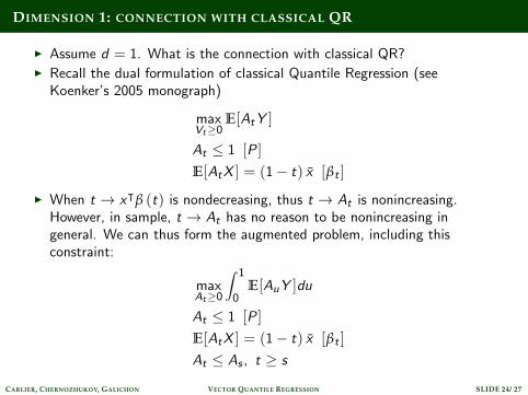
DIMENSION 1: CONNECTION WITH CLASSICAL QR

I Assume d = 1. What is the connection with classical QR?I Recall the dual formulation of classical Quantile Regression (see

Koenker’s 2005 monograph)

maxVt≥0

E[AtY ]

At ≤ 1 [P ]

E[AtX ] = (1− t) x [βt ]

I When t → xᵀβ (t) is nondecreasing, thus t → At is nonincreasing.However, in sample, t → At has no reason to be nonincreasing ingeneral. We can thus form the augmented problem, including thisconstraint:

maxAt≥0

∫ 1

0E[AuY ]du

At ≤ 1 [P ]

E[AtX ] = (1− t) x [βt ]

At ≤ As , t ≥ s


VQR: CONNECTION WITH CLASSICAL QR

I Theorem: this problem is equivalent to VQR.

I Indeed, let U =∫ 10 Aτdτ. One has At = 1 {U ≥ t} for t ∈ [0, 1], and

the previous problem rewrites

maxU

E[UY ]

E[1 {U ≥ t}X ] = (1− t) x ∀t ∈ [0, 1]

or alternatively

maxU

E[UY ]

U ∼ U ([0, 1]) , E[X |U ] = x

which is VQR. Dual variable b is recovered via b (t) =∫ t0 βτdτ.


CONNECTION WITH CLASSICAL QR: QUASI-SPECIFICATION

I Question: why mean-independence plays a role in QR?

I Definition: QR is quasi-specified if t → x> βQRt is increasing for all x ,

i.e. if there is no “crossing problem”.

I Theorem: if QR is quasi-specified, then there is a representation

Y = X> βQRU , U ∼ U ([0, 1]) , E[X |U ] = x .

I Proof: there exists t (x , y) such that x> βQRt(x,y )

= y . Letting

U = t (X ,Y ), one has Y = X> βQRU ; but

1 {U ≥ t} = 1{Y ≥ X> βQR

t

}, hence E[X1 {U ≥ t}] = x (1− t),

QED.


REMAINING AGENDA

I Empirical application in progress: hedonics models (real estate prices;wine prices). Possible other applications to measures of financial risk.

I Numerical methods: auction algorithm; entropic regularization...

I Sparse versions when vector of covariates X is high-dimensional.


Documents

Alfred Galichon (NYU Econ+Math) Based on joint works with