Algebra 2

Notes by Charles Lynch of a course given byTim Dokchitser (2016), edited by TD

May 21, 2018

We open the course by briefly talking about what “Algebra” is. Basically, it isthe study of abstract structures and operations. Three of these structures arefundamental in modern algebra:

• We have groups, which you met last year, which have a single binaryoperation ×. Examples of groups are Cn and Sn.

• We have rings, which have addition, subtraction and multiplication. Ex-amples of rings are Z and R[x].

• We also have fields, which have addition, subtraction, multiplication anddivision. Examples of fields are Q, R and C.

We normally teach algebra by starting with groups, introducing rings and thenbuilding up to fields — however, ironically, this means we start with hardestand least natural of these three structures. Most people are quite familiar withfields (even though they do not know they are called fields) but find groupsrather abstract.

In this course, we focus on rings, delve into fields and briefly consider applica-tions to ruler and compass constructions at the end.

1

Contents

1 Rings 31.1 New Rings From Old . . . . . . . . . . . . . . . . . . . . . . . . . 51.2 Product Rings . . . . . . . . . . . . . . . . . . . . . . . . . . . . 7

2 Isomorphisms and Homomorphisms 92.1 Homomorphisms . . . . . . . . . . . . . . . . . . . . . . . . . . . 122.2 Quotient Rings . . . . . . . . . . . . . . . . . . . . . . . . . . . . 15

3 Fundamental Properties 183.1 Integers . . . . . . . . . . . . . . . . . . . . . . . . . . . . . . . . 203.2 Ideals, Fields, Homomorphisms . . . . . . . . . . . . . . . . . . . 20

4 Integral Domains and Fields 244.1 Maximal and Prime Ideals . . . . . . . . . . . . . . . . . . . . . . 27

5 Principal Ideal Domains, Euclidean Domains, Unique Factori-sation Domains 315.1 Noetherian rings . . . . . . . . . . . . . . . . . . . . . . . . . . . 315.2 Primes and Irreducibility . . . . . . . . . . . . . . . . . . . . . . 335.3 UFDs . . . . . . . . . . . . . . . . . . . . . . . . . . . . . . . . . 355.4 Highest Common Factor . . . . . . . . . . . . . . . . . . . . . . . 365.5 Principal Ideal Domains . . . . . . . . . . . . . . . . . . . . . . . 375.6 Polynomial Rings over a Field . . . . . . . . . . . . . . . . . . . . 40

6 Field Extensions, Gauss’ Lemma and Consequences 436.1 Gauss’ Lemma . . . . . . . . . . . . . . . . . . . . . . . . . . . . 43

7 Testing Polynomials for Irreducibility 48

8 Fields 558.1 Subfields and Extensions . . . . . . . . . . . . . . . . . . . . . . . 568.2 Characteristic of a Field . . . . . . . . . . . . . . . . . . . . . . . 578.3 Algebraic and Transcendental Elements . . . . . . . . . . . . . . 64

9 Finite Fields 689.1 Examples of Finite Fields . . . . . . . . . . . . . . . . . . . . . . 68

10 Ruler and Compass Constructions 75

2

1 Rings

Definition 1.1 (Ring). A ring is a set R together with 2 binary operations -operations that take two elements and produce one - called addition and mul-tiplication, and denoted by + and · (or ×) respectively, such that, ∀a, b, c ∈ R,the two operations are

• Commutative; that is, a+ b = b+ a, and ab = ba.

• Associative; that is, (a+ b) + c = a+ (b+ c), and (a · b) · c = a · (b · c).

• Distributive; that is, (a+ b) · c = a · c+ b · c.

and such that

• There is a zero element 0 ∈ R such that a+ 0 = a ∀a ∈ R;

• There is a unit element1 1 ∈ R such that a · 1 = a ∀a ∈ R;

• Every a ∈ R has an additive inverse −a ∈ R such that a+ (−a) = 0.

For x, y elements of a ring, we often simply write xy for x · y and x − y forx+ (−y). It follows easily from the axioms that the zero element and additiveinverse are both unique (see below).

We now look at some examples of rings, to get a better understanding of whatthey are like;

Example 1.2.

• R = Z, the integers, is an example of a ring, with the usual +,−,×, 0, 1.

• Similarly, Q, the rationals, R, the reals, and C, the complex numbers, areall examples of rings.

• R = R[x], polynomials in x with real coefficients, is a ring.

• For a less obvious example, R = {functions : R → R}, the set of func-tions mapping from the reals to the reals, is a ring. Similarly, the set ofcontinuous functions, or differentiable functions, are also rings.

• Trivially, we also have ‘the zero ring’ R = {0} with 0 + 0 = 0 · 0 = −0 = 0and 1 = 0. It satisfies all ring axioms as well.2

We now aim to establish some basic, natural facts about rings.

Proposition 1.3. Let R be a ring with zero element denoted by 0, and multi-plicative identity denoted by 1. Then

1. If z ∈ R such that ∀a ∈ R, z + a = a, then z = 0; that is, zero is unique.

1also sometimes called ‘multiplicative unit’ or ‘multiplicative identity’. We will usuallyjust call it ‘One’, because the word ‘unit’ is used for any element of the ring that has amultiplicative inverse — see below.

2However, it is an annoying exception to half of the results about rings, even worse thanthe empty set in set theory. So many of our theorems will start with ‘Let R 6= {0} be a ring...’

3

2. If u ∈ R such that ∀a ∈ R, u · a = a, then u = 1; that is, 1 is unique.

3. If a, b, c ∈ R such that a+ b = 0 and a+ c = 0, then b = c; that is, −a isunique.

4. 0 · a = 0 ∀a ∈ R.

5. With −1 the additive inverse of 1, we have that ∀a ∈ R,−1 · a = −a.

6. For a ring R, 0 = 1 if and only if R = {0}.

Proof. We leave most of these results as an exercise.

However, to whet your appetite, we prove statement (c) as follows;

a+ b = a+ c

=⇒ −(a) + (a+ b) = −a+ (a+ c)

=⇒ (−a+ a) + b = (−a+ a) + c

=⇒ 0 + b = 0 + c

=⇒ b = c.

Hence statement (c) holds.

Notation 1.4. For a, b ∈ R and n ∈ N, we establish the following notation:

• We write a− b for a+ (−b);

• We write an for a · a · · · · · a, n times;

• We write 2a for a+ a;

• We write −2a for −a− a, etc.

Remark 1.5. Many books define rings with more relaxed conditions, whereinmultiplication is not necessarily commutative, and the multiplicative unit maynot exist. Then R = M2(R), the set of 2× 2 matrices (non-commutative), andR = 2Z, the even integers (no multiplicative unit), also become rings. In thismore general terminology, what we called a ring is called ‘a commutative ringwith unity’.

Note that for a ring, if we ignore multiplication and 1, then (R,+,−, 0) is anabelian group.

As opposed to the additive inverse, in general, most r ∈ R have no multiplicativeinverse. This leads us nicely to our next definition.

Definition 1.6 (Unit). Let R be a ring, and take r ∈ R. If ∃s ∈ R suchthat rs = 1, then r is called a unit, and s is denoted by r−1, said to be themultiplicative inverse of r.

As an exercise, show that such an s, if it exists, is unique.

4

Notation 1.7. We write R× to be the set of units in R. This set forms anabelian group under multiplication.

Example 1.8. We consider several rings and their set of units.

R = Z, R× = {±1}R = Q, R× = Qr {0}R = R, R× = Rr {0}R = R[x], R× = Rr {0}R = {functions : R→ R}, R× = {nowhere zero functions : R→ R}

For examples of such nowhere zero functions, consider f(x) = x2+1 and f(x) =1/(x2 +1), and for non-examples, consider f(x) = x and f(x) = 1/x - the latterof which is not a function R→ R, as it is undefined at x = 0.

Some of the rings, like Z above, have very few units. Some of the others goto an opposite extreme - the set of units is the same as the whole ring with 0removed. This is the most important class of rings:

Definition 1.9. A ring R 6= {0} is called a field if every nonzero element of Ris a unit.

Example 1.10. Because of this definition, Q,R and C are all classed as fields,whereas Z,R[x], and the set of functions mapping reals to reals are not fields.

In a field a/b (defined as ab−1) makes sense for any a, b with b 6= 0, so we oftensay that ‘in a ring we have +,−,× and in a field +,−,×, /’.

Example 1.11 (Integers modulo n). For an integer n ≥ 1 (‘modulus’), consider

R = Z/nZ := {residue classes mod n} = {0, 1, . . . , n− 1}.

The operations of addition and multiplication modulo n make it into a ring:

a+ b = a+ b mod n,

a · b = ab mod n.

Example 1.12. For n = 2, we have that R = {0, 1}.

For n = 10, we have that R = {0, 1, . . . , 8, 9}.

Exercise 1.13. The units of Z/10Z are (Z/10Z)× = {1, 3, 7, 9}, and moregenerally, (Z/nZ)× = {a : a coprime to n}. In particular, Z/nZ is a field if andonly if n is a prime number.

1.1 New Rings From Old

We now look at how we can obtain new rings from existing ones.

5

Definition 1.14 (Subring). Let (R,+,−,×, 0, 1) be a ring. A subset S ⊂ R isa subring of R if 0, 1 ∈ S and (S,+,×) itself is a ring.

Lemma 1.15. We have that S ⊂ R is a subring if, and only if, S is closedunder addition, multiplication and additive inverses, and 1 ∈ S.

Proof. Not hard.

Example 1.16. Some simple examples of subrings are Z ⊂ Q ⊂ R ⊂ C, andalso R ⊂ R[x], constant polynomials inside all polynomials.

We have that 2Z ⊂ Z is not a subring, as 2Z, the even integers, does not containunity.

Furthermore, 1 + 2Z ⊂ Z, the odd integers, is not a subring, as it has no zeroelement and is also not closed under addition.

Finally, {0, 1} ⊂ Z is not a subring, as it is not closed under addition.

Example 1.17. Z[i] ⊂ C, i =√−1 ∈ C, the Gaussian integers, is defined as

Z[i] = {a+ bi : a, b ∈ Z},

and is a subring of C.

This is true as clearly 1 ∈ Z[i], and we can show that it is closed under addition,multiplication and additive inverses.

Exercise 1.18. You can show that the units of the Gaussian integers areZ[i]× = {1,−1, i,−i}. As an abelian group, this is a cyclic group of order 4.

Remark 1.19. This Z[i] is the smallest possible subring of C containing i.That is, every subring R ⊂ C containing i must contain the whole of Z[i]. Thisholds due to the fact that a subring must also contain 1, and be closed underaddition and additive inverses, which implies Z[i] ⊂ R.

Generally, for α ∈ C, we can write

Z[α] = smallest subring of C containing α

= set of complex numbers that are generated from 1, α using +,−,×= polynomial expressions a0 + a1α+ . . .+ anα

n with n ≥ 0, ai ∈ Z

Even more generally, suppose R is any ring, which is a subring of some ring S,and α ∈ S. Then we write

R[α] = smallest subring of S containing R and α

= elements of S that are generated from all r ∈ R and α using +,−,×= polynomial expressions a0 + a1α+ . . .+ anα

n with n ≥ 0, ai ∈ R

Later, for fields K ⊂ F and α ∈ F we will also introduce a similar notation K(α)for the smallest field containing K and α. It is a field of rational expressions(quotients of two polynomials) in α, with coefficients in K.

6

1.2 Product Rings

Definition 1.20 (Product Rings). Let R,S be rings. The cartesian product3

R × S = {(r, s) : r ∈ R, s ∈ S} can be given a ring structure, called a productring, by component wise +,−,×;

(r, s) + (r′, s′) = (r + r′, s+ s′)

and(r, s) · (r′, s′) = (rr′, ss′)

We have that zero is (0, 0) and the multiplicative identity is (1, 1).

Clearly this satisfies all the axioms as R and S satisfy all the axioms, and wehave defined this ring component wise.

Example 1.21. Taking R = S = Z, then Z × Z = {(a, b) : a, b ∈ Z}. As anabelian group under addition it is the same as Gaussian Integers, but multipli-cation is completely different.

Proposition 1.22. Let R,S be rings. (R× S)× = R× × S×.

Proof. We observe that

(r, s) is a unit ⇐⇒ ∃(r′, s′) ∈ R× S such that (r, s)(r′, s′) = (1, 1)

⇐⇒ (rr′, ss′) = (1, 1)

⇐⇒ rr′ = 1 = ss′

⇐⇒ r ∈ R×, s ∈ S×

Which is what we set out to prove.

We now focus fire on polynomials.

Definition 1.23. Let R be a ring, and x a symbol. Define

R[x] := {polynomial expressions a0 + a1x+ . . .+ anxn : ai ∈ R,n ∈ Z≥0}.

We say that a polynomial as above has degree n. Then R[x] is a ring under theusual addition, multiplication and additive inverse.

Example 1.24. The usual polynomials are of the form Z[x],R[x], respectivelyhaving elements of Z and R as coefficients.

For polynomial rings, we have R[x, y] = R[x][y].

Example 1.25. Consider the integers modulo 2; Z/2Z = {0, 1}, or {0, 1}.3Some books will denote R× S by R⊕ S as well, but we will never do this

7

Then

Z/2Z[x] = {polynomials with coefficients ai ∈ Z/2Z}= {0, 1, x, x+ 1, x2, x2 + 1, x2 + x, . . .}

(Note that the degree of such a polynomial is a usual integer 0, 1, 2, 3, ..., not aninteger modulo 2; only the coefficients are. For example, x1 and x3 are differentelements of our ring.)

To exemplify operations in such a ring, note that

(x+ 1) + (x2 + 1) = x2 + x (as 1 + 1 = 0)

(x+ 1)2 = x2 + 2x+ 1 = x2 + 1

(x+ 1)4 = (x2 + 1)2 = x4 + 2x2 + 1 = x4 + 1

Finally, we note that the set of functions also forms a ring:

Exercise 1.26. Let R be a ring, and X an arbitrary set. Then

F = {functions f : X → R}

naturally form a ring.

8

2 Isomorphisms and Homomorphisms

We now turn to maps between rings.

Definition 2.1. Let R,S be rings. A map ϕ : R→ S is a ring isomorphism if

1. ϕ is bijective;

2. ϕ preserves +,×; that is, ∀a, b ∈ R,

ϕ(a+ b) = ϕ(a) + ϕ(b)

ϕ(ab) = ϕ(a)ϕ(b)

(We could also add that ϕ(0) = 0, ϕ(1) = 1 and ϕ(−a) = −ϕ(a), but thesefollow automatically from conditions 1 and 2.)

If such an isomorphism exists, we say that R and S are isomorphic, and wewrite R ∼= S.

Remark. It it easy to check that if φ : R→ S is an isomorphism, then so is itsinverse φ−1 : S → R.

Example 2.2. The Boolean ring with 2 elements,

B = {False, True} with r + s = r XOR s, rs = r AND s.

We can find the results of these operations by looking at the relevant truthtables. Not only is this a ring, but it is isomorphic to Z/2Z, by mapping falseto 0 and true to 1.

Example 2.3. Consider the identity map

ϕ1 : C→ Ca+ bi 7→ a+ bi

It is trivially an isomorphism. Complex conjugation is also an isomorphism:

ϕ2 : C→ Ca+ bi 7→ a− bi,

as it preserves addition and multiplication, and is a bijection as well.

Exercise 2.4 (Quite hard). The only isomorphism ϕ : R→ R is identity.(Hint. Steps: (1) identity on Z; (2) identity on Q; (3∗) identity on R;)

Example 2.5 (Fake Complex Numbers). We define complex numbers as C ={a + bi : a, b ∈ R}, with i2 = −1. However, we can also define ‘fake’ complexnumbers by defining i2 differently; say, i2 = −4, i2 = 1, i2 = π, i2 = i+ 1. Eachsuch choice leads to a ring, and a natural question that arises is whether thiswill still define C, or whether it will result in an entirely different ring.

9

Let C = {a+ bx : a, b ∈ R}, a 2-dimensional real vector space with basis {1, x}.Can we make C into a ring such that R ⊂ C is a subring?

Well, if we want R = {a+ 0x} to sit inside C as a subring, from ring axioms wehave to take

a+ bx+ c+ dx := (a+ c) + (b+ d)x

−(a+ bx) := −a− bx(a+ bx)(c+ dx) = ac+ (bc+ ad)x+ bdx2

The only question we have to settle is: what is x2?

As mentioned above, we usually take x2 = −1, but in principle we could pickany other element of t ∈ C for x2 as well.

It is fairly easy4 to check that each choice gives a ring Ct,

C−1, C0, C−4, C1, Cπ, Cx+1, C3x−2, . . .

For example:

• C−1 = {a + bx : a, b ∈ R} with x2 = −1 is isomorphic to C, the usualcomplex numbers. In other words, ‘x = i’.

• C−4 = {a+ bx : a, b ∈ R} with x2 = −4 is once again isomorphic to C, ifwe map a+ bx to a+ b(2i). In other words, ‘x = 2i’.

• In general, for real α < 0, we have that Cα ∼= C−1, mapping x to√αi. This

is also why we normally define i2 = −1 as opposed to another negativenumber; i2 = −1 is merely the simplest of all the options, but they allgive the same ring.

• Similarly, we have that for α > 0, Cα ∼= C1.

What about the general ring, R = Cαx+β ; in other words, when we take x2 =αx+ β for some α, β ∈ R? We consider in R

x2 − αx− β = 0

(x− α

2)2 − α2

4− β = 0

We could declare the first term to be ’new x’, and D = α2

4 + β, then x2 = D.

In other words, we have the isomorphism

Cαx+β ∼= CD

x 7→ x+α

24Checking that multiplication is associative is the only tedious one

10

Now D is real, either > 0 or < 0 or = 0, and we are down to three rings:

• C−1 = {a+ bx : a, b ∈ R} with x2 = −1;

• C1 = {a+ bx : a, b ∈ R} with x2 = 1;

• C0 = {a+ bx : a, b ∈ R} with x2 = 0.

They are in fact non-isomorphic to one another, and furthermore...

Proposition 2.6. C1∼= R× R.

Proof. We find an isomorphism by trying to match some special elements first.For R × R, we consider the basis vectors e1 = (1, 0) and e2 = (0, 1), whichsatisfy e1 + e2 = 1, e1e2 = 0, e21 = e1, and e22 = e2.

Any isomorphism

ϕ : R× R→ C1

e1 7→ ϕ(e1)

e2 7→ ϕ(e2)

takes them to elements that satisfy the same relations, as all the operations arepreserved. So ϕ(e1)2 = ϕ(e1), ϕ(e2)2 = ϕ(e2), e1 + e2 = 1→ ϕ(e1 + e2) = ϕ(1),and ϕ(e1) + ϕ(e2) = 1.

So we need to find elements in C1 such that these hold.

As x2 = 1, try, say 1± x first:

(1 + x)2 = 2 + 2x

(1− x)2 = 2− 2x

(1 + x) + (1− x) = 2

(1 + x)(1− x) = 1 = x2 = 1− 1 = 0

Which is almost what we want, just out by a factor of 2. Since we don’twant the 2s, we rescale by 2, and take v1 = 1+x

2 and v2 = 1−x2 , which are

indeed the elements we’re looking for - and it is easy to check that we get anisomorphism.

So to summarise, there are three essentially different ways to define “fake com-plex numbers”;

C = {ax+ b : a, b ∈ R} with x2 ∈ {−1, 0, 1}−1 =⇒ usual C;

1 =⇒ R× R;

0 =⇒ a ring known as the “dual numbers”.

11

Note that the latter 2 of these 3 rings are far from nice, as they have ‘zerodivisors’ - that is, elements a, b ∈ R such that a 6= 0, b 6= 0, but ab = 0.

As examples of such zero divisors, in C1, (1 + x)(1− x) = 0, and in C0, x2 = 0.

Incidentally, this makes it clear that C0 � C and C1 � C, as C has no zerodivisors.

Furthermore, C0 � C1, because in C0 we have that x2 = 0, but in C1 there areno nonzero elements that square to 0, because C1

∼= R×R, so (a, b)2 = (a2, b2),and (a2, b2) 6= 0 unless a = b = 0. So these 3 rings are genuinely different.

2.1 Homomorphisms

We now move on to the more general maps:

Definition 2.7 (Homomorphisms). Let R,S be rings. A map ϕ : R→ R′ is a(ring) homomorphism if, ∀a, b ∈ R, we have

ϕ(1) = 1

ϕ(a+ b) = ϕ(a) + ϕ(b)

ϕ(ab) = ϕ(a)ϕ(b)

(It is not hard to check that ϕ(0) = 0 and ϕ(a − b) = ϕ(a) − ϕ(b) hold auto-matically in this case - see proposition below.)

So a homomorphism is a more general form of an isomorphism, or alternatively,an isomorphism is just a bijective homomorphism.

Example 2.8. Every ring isomorphism is also a ring homomorphism. Forinstance, complex conjugation on C

ϕ : C→ Cz 7→ z

is a homomorphism, as well as the identity map ψ : C→ C (or identity R→ Rfor any other ring R).

Example 2.9. Every subring S of a ring R defines a homomorphism, given byinclusion S ⊂ R;

ϕ : S ↪→ R

To exemplify this, we have that Z ↪→ Q,R ↪→ C, and R ↪→ R[x] are ringhomomorphisms.

Example 2.10. Consider

ϕ1 : Z→ Z/2Za→ a mod 2

12

This is a homomorphism of rings, mapping all the even numbers to 0 and allthe odd numbers to 1. This generalises to Z/nZ for any n ≥ 1.

Example 2.11 (Evaluating polynomials).

ϕ : R[x]→ Rf(x) = anx

n + . . .+ a0 7→ a0 = f(0)

is a homomorphism, and so is f 7→ f(1), or f 7→ f(π).

Proposition 2.12. Let R,S be rings, ϕ : R → S a homomorphism. Then wehave that

(a) ϕ(0) = 0;

(b) ∀a ∈ R, ϕ(−a) = −ϕ(a);

(c) The image ϕ(R) = {ϕ(a) : a ∈ R} is a subring of S;

(d) If ψ : S → T is another homomorphism, the composition ψ ◦ ϕ : R → Tis a homomorphism as well.

Proof. (a) Note that in R, we have 0 = 0 + 0. So in S,

ϕ(0) = ϕ(0 + 0) = ϕ(0) + ϕ(0).

Adding −ϕ(0) to both sides of this equation gives us 0 = ϕ(0).

(b) Take a ∈ R. We have

ϕ(−a) + ϕ(a) = ϕ(−a+ a) = ϕ(0) = 0.

Thus in S, ϕ(−a) is the additive inverse of ϕ(a), meaning that ϕ(−a) = −ϕ(a).

(c) 1 ∈ ϕ(R), ϕ(R) is closed under addition and multiplication, and we haveϕ(a) + ϕ(b) = ϕ(a+ b), so it is a subring.

(d) We have that a, b ∈ R =⇒ ψ(ϕ(a+b)) = ψ(ϕ(a)+ϕ(b)) = ψ(ϕ(a))+ψ(ϕ(b))and similarly for multiplication and 1.

Definition 2.13 (Kernel). Suppose R,S are rings and ϕ : R → S is a homo-morphism. We define kerϕ, the kernel of ϕ, by

kerϕ = {a ∈ R : ϕ(a) = 0}.

Take note of something very important; the kernel of a linear map of vectorspaces is itself a vector space, the kernel of a homomorphism between groups isitself a group, but the kernel of a ring homomorphism is not necessarily a ring:

13

Example 2.14. For

ϕ1 : Z→ Z/2Zn→ n mod 2

we have that kerϕ = {n ∈ Z : ϕ(n) = 0} = 2Z, the even integers.

Furthermore, for

ϕ : R[x]→ Rf(x) = anx

n + . . .+ a0 7→ a0 = f(0)

then the kernel is

kerϕ = {polynomials with f(0) = 0}= {polynomials of the form xg(x)}

In both examples, kerϕ is not a ring, as it does not contain unity (though itsatisfies all the other ring axioms).

To understand these kernels, we introduce the concept of an “ideal”.

Definition 2.15 (Ideal). Let R be a ring, I ⊂ R. We say I is an ideal of R if

(a) I is an additive subgroup of R; that is, 0 ∈ I and I is closed under additionand additive inverses;

(b) ∀r ∈ R, i ∈ I, we have that r · i ∈ I.

The missing condition from being a ring is that we do not ask for 1 ∈ I. Con-dition (b) is sometimes described as I being closed under multiplication byelements of R, which is stronger than just being closed under ×.

Proposition 2.16. Let ϕ : R → S be a ring homomorphism. Then kerϕ ⊂ Ris an ideal.

Proof. Immediately we see that ϕ(0) = 0, so 0 ∈ kerϕ. Furthermore, we notethat if we have ϕ(a) = 0 and ϕ(b) = 0, then ϕ(a + b) = ϕ(a) + ϕ(b) = 0. Sokerϕ is closed under addition. We also have that for any a ∈ R, if ϕ(b) = 0,then ϕ(ab) = ϕ(a)ϕ(b) = 0, so ab ∈ kerϕ and hence kerϕ is closed undermultiplication. As it is closed under addition and multiplication, it follows thatit is closed under additive inverses.

Example 2.17. While 2Z is not a ring, we have that 2Z ⊂ Z is an ideal.Beyond this, it is the case that nZ ⊂ Z is an ideal for all n ≥ 1. Trivially, wealso have that {0} ⊂ Z is an ideal.

Proposition 2.18. Let ϕ : R→ S be a homomorphism. Then ϕ is injective ifand only if kerϕ = {0}.

14

Proof. Suppose ϕ is injective. Since ϕ(0) = 0, we have that ϕ(a) 6= 0 for anya 6= 0, so kerϕ = {0}.

Now say kerϕ = {0}, and suppose ϕ(a) = ϕ(b). Then

0 = ϕ(a)− ϕ(b) = ϕ(a− b).

Thus (a−b) ∈ kerϕ, and since kerϕ = {0}, this means a−b = 0, or equivalently,a = b. So ϕ is injective.

Example 2.19. Consider R = Z/4Z = {0, 1, 2, 3}, and S = Z/2Z = {0, 1}.

There is a homomorphism R → S defined by n 7→ n mod 2, but there are nohomomorphisms S → R, since 1 + 1 = 0 in S, but ψ(1) + ψ(1) 6= ψ(0) in R.

More generally, there is a natural homomorphism Z → Z/nZ taking x 7→ xmod n, but there are no homomorphisms Z/nZ→ Z.

We classify this idea more formally in the following lemma.

Lemma 2.20. Let R be a ring, and r ∈ R an arbitrary element satisfying analgebraic equation of the form

anrn + . . .+ a1r + a0 = 0

with integers ai (viewed as elements of R). Then under any homomorphismϕ : R→ S, we have that ϕ(r) satisfies the same equation.

Proof. By definition of ϕ, we have that 0 → 0, 1 → 1, addition, multiplicationand additive inverses are preserved, and so this result is clear.

Example 2.21. There are no ring homomorphisms ϕ : C → R, since we havethat i satisfies x2 + 1 = 0, but there is no such element in R.

Similarly, we can tell that there are no ring homomorphisms ψ : R → Q, bythinking of a parallel argument involving

√2.

2.2 Quotient Rings

We now focus on the following goal: with R a ring, and I an ideal, we want toconstruct a quotient ring R/I. We begin with its elements, ‘cosets of I’:

Definition 2.22 (Coset). Let I be an ideal of a ring R. Let r ∈ R be arbitrary.The coset of r modulo I is the set of elements5

r + I := {r + i : i ∈ I}5 We do not need to differentiate between ‘left cosets’ r+ I and ‘right cosets’ I + r because

addition is commutative.

15

If for r, s ∈ R, we introduce a relation

r ∼ s ⇐⇒ r − s ∈ I,

then it is an equivalence relation (because 0 ∈ I and I is closed under additionand additive inverses), with the equivalence classes being precisely the cosets.

Example 2.23. For R = Z, I = 4Z, we have that

I = . . . ,−4, 0, 4, 8, . . .

1 + I = . . . ,−3, 1, 5, 9, . . .

2 + I = . . . ,−2, 2, 6, 10, . . .

3 + I = . . . ,−1, 3, 7, 11, . . .

There are 4 different cosets, the equivalence classes for

r ∼ s ⇐⇒ r ≡ s mod 4.

So 2 + I = 6 + I, 3 + I = −1 + I, etc.

Definition 2.24 (Quotient Ring). The set of cosets, denoted R/I, is called thequotient ring of R by I.

We justify the word ‘ring’ with the following theorem.

Proposition 2.25. We have that R/I is a ring, under

(a+ I) + (b+ I) := (a+ b) + I

(a+ I)(b+ I) := ab+ I

with I = 0 + I as the zero element, with 1 + I as 1, and −(a+ I) = (−a) + I.

Example 2.26. Briefly demonstrating the ideas behind this, from our previousexample take6

I = . . . ,−4, 0, 4, 8, . . .

a+ I = . . . ,−3, 1, 5, 9, . . .

b+ I = . . . ,−2, 2, 6, 10, . . .

The sum of a+ I and b+ I is the coset

(a+ b) + I = . . . ,−5,−1, 3, 7, 11, . . . .

Proof of proposition. The main point here is to show that addition and multi-plication are well-defined on cosets - so if a′ = a+ i1, b′ = b+ i2, for i1, i2 ∈ I,then

(a′ + b′) + I = a+ b+ i1 + i2 + I = (a+ b) + I

a′b′ + I = ab+ ai2 + bi1 + i1i2 + I = ab+ I

Associativity, commutativity, distributivity etc. are all clear from this.6 Pick a = 1, b = 2 or a = 9, b = −2, ...

16

Example 2.27.

• Take R = Z, I = nZ with n ≥ 1 an integer. Then R/I = Z/nZ, theintegers modulo n.

• For any R, with I = {0}, we have that R/I ∼= R, with a+ (0) 7→ a.

• Similarly, for any R, with I = R, then R/I ∼= {0} is the zero ring.

17

3 Fundamental Properties

Theorem 3.1 (Fundamental Homomorphism Theorem7). Let ϕ : R → S be aring homomorphism, with kerϕ = I. Then R/I ∼= ϕ(R); that is,

R/ kerϕ ∼= imϕ.

Proof. Define a map

ϕ : R/I → ϕ(R)

r + I → ϕ(r)

We have that this is

• Well-defined; r′ ∈ r + I implies that r′ = r + i for some i ∈ I, and soϕ(r′) = ϕ(r) + ϕ(i).

• A Homomorphism; this clearly preserves addition, multiplication and ad-ditive inverses, and ϕ(1 + I) = ϕ(1) = 1.

• Surjective; every element s ∈ ϕ(R) is of the form s = ϕ(r), by definitionof ϕ(r), for some r ∈ R. So ϕ(r + I) = s.

• Injective; if ϕ(r+ I) = 0, then ϕ(r) = 0 implies r ∈ I, and so r+ I = 0+ Ias I = kerϕ.

And so the theorem holds.

Example 3.2. Consider ϕ1 : R → R, the identity homomorphism. We havethat kerϕ = {0} and imϕ = R, so R/{0} ∼= R.

Consider ϕ2 : R → {0}, with kerϕ = R and imϕ = {0}. We see that R/R ={0}.

For ϕ3 : R[x]→ R, with f(x) 7→ f(0), we

kerϕ = {polynomials of the form x · g(x)} = xR[x], imϕ = R,

so we see that R[x]/xR[x] ∼= R.

For ϕ4 : Z→ Z/nZ defined by a 7→ a mod n, we have that kerϕ = nZ, and asthis is surjective, we have that Z/nZ ∼= Z/nZ - which justifies our notation forthe integers modulo n.

Finally, for ϕ5 : Z/4Z → Z/2Z, we have that kerϕ = {0, 2} and imϕ = Z/2Z,so Z/4Z/{0, 2} = Z/2Z.

Example 3.3. Let

ϕ2 : Z→ Z/2Zn 7→ n mod 2

7Also called ‘First Isomorphism Theorem’

18

and

ϕ3 : Z→ Z/3Zn 7→ n mod 3

be ring homomorphisms. We combine these to obtain

ϕ23 : Z→ Z/2Z× Z/3Zn 7→ (n mod 2, n mod 3).

which is clearly also a homomorphism, with kerϕ23 = 6Z (as clearly 2|n and3|n if and only if 6|n). In detail,

kerϕ23 = {n ∈ Z : ϕ23(n) = (0, 0)}= {n ∈ Z : n mod 2 = 0 ∧ n mod 3 = 0}= {n ∈ Z : 2|n ∧ 3|n}= {n ∈ Z : 6|n}= 6Z.

By the above theorem, we obtain that

Z/6Z ∼= image of ϕ23 ⊂ Z/2Z× Z/3Z

and by comparing sizes, we see that ϕ23 is surjective, and so Z/6Z ∼= Z/2Z ×Z/3Z. In particular, ϕ is surjective, i.e. for every (a, b) ∈ Z/2Z × Z/3Z, thereexists some n ∈ Z such that

n mod 2 = a

n mod 3 = b

Which is precisely the Chinese Remainder Theorem for 2 and 3.

What if we generalised the above to m and n, instead of 2 and 3?

Theorem 3.4. If m,n ≥ 1 are coprime, then

Z/mnZ ∼= Z/mZ× Z/nZ

Proof. Same argument.

Remark 3.5. If m and n are not coprime, then the two rings Z/mnZ andZ/mZ × Z/nZ are not isomorphic; it is quite instructive to take, for instance,m = n = 2 and verify this.

19

3.1 Integers

Let us classify all ideals of Z:

Proposition 3.6.

(a) Every ideal of Z is of the form nZ, for some integer n ≥ 0.

(b) Every ring R admits a unique ring homomorphism Z→ R.

(c) Every ring R either contains Z or a unique Z/nZ, for some n ≥ 1, as asubring.

Proof. We leave the first two parts of this proposition as an exercise. (Hint: (a)If I ⊂ Z is an non-zero ideal, take the smallest positive integer n that lies in Iand show that I = nZ using division with remainder; (b) 0→ 0, 1→ 1 and thisdetermines the homomorphism uniquely.)

For part (c), let ϕ : Z→ R be the unique homomorphism, and let I = kerϕ ⊂ Z.Then either

I = Z =⇒ imϕ = {0} =⇒ R = {0}.I = {0} =⇒ imϕ ∼= Z ↪→ R subring.

I = nZ =⇒ imϕ ∼= Z/nZ ↪→ R subring,

with the last part following from the fundamental homomorphism theorem.

Example 3.7. Z,Q,R,C,Z[x], {differentiable functions : R→ R} all contain Zas a subring, and that Z/2Z,Z/2Z× Z/2Z,Z/2Z[x] all contain Z/2Z.

3.2 Ideals, Fields, Homomorphisms

Proposition 3.8. Let I, J ⊂ R be ideals. Then

1. I ∩ J is an ideal;

2. I + J = {i+ j : i ∈ I, j ∈ J} is an ideal;

3. IJ = {finite sums∑nk=1 ikjk : ik ∈ I, jk ∈ J} is an ideal.

Proof. The proof is left as an exercise.

Example 3.9. Consider the case where R = Z, I = mZ, and J = nZ. Then wehave that

IJ = mnZI + J = hcf(m,n)ZI ∩ J = lcm(m,n)Z

Lemma 3.10. Let I ⊂ R be an ideal. If I contains a unit r ∈ R×, then I = R.

20

Recall that a unit r is an element r ∈ R such that ∃r′ ∈ R with rr′ = 1. SoI = R is sometimes called the unit ideal because of this.

Proof. Since rr′ = 1, and r ∈ I, we have that rr′ = 1 ∈ I. Now for any s ∈ R,we have s = s · 1 ∈ I, so I = R.

This leads us nicely into the following theorem;

Theorem 3.11. A ring R 6= {0} is a field if and only if {0} and R are the onlyideals of R.

Proof. For the forward direction, since R is a field, we have that the units areR× = R r {0}. So every ideal I 6= {0} contains a unit, and by the lemma,I = R.

For the backwards direction, pick r ∈ R, r 6= 0. We want to show that everyr 6= 0 has a multiplicative inverse. So let I = {rx : x ∈ R}, which is clearly anideal not equal to {0}. By our assumption, I = R. So 1 ∈ I =⇒ 1 = rx forsome x ∈ R. Hence r is a unit.

Example 3.12. Consider R = Q,R,C. These are all fields, and so have {0}and R as their only ideals. On the other hand, the following 4 rings all haveother ideals, and hence are not fields.

R = Z, I = 2ZR = R[x], I = xR[x]

R = R× R, I = R× {0}R = Z/4Z, I = {0, 2}

Corollary 3.13. Let ϕ : R → S be a ring homomorphism, S 6= {0}. If R is afield, then ϕ is injective.

Proof. R has {0} and R as the only ideals. Either kerϕ = R =⇒ S = {0}, asϕ(1) = 1 =⇒ 1 = 0 in S, or kerϕ = {0} =⇒ ϕ is injective.

Example 3.14. Q ↪→ R is a ring homomorphism, but there are no ring homo-morphisms of the form R→ Q, since the reals are uncountable but the rationalsare countable, and there are no injections from an uncountable set to a countableset.

Theorem 3.15. Let ϕ : R � R′ be a surjective ring homomorphism; that is,R/ kerϕ ∼= R′ (by the Fund. Hom. Thm.). Then

(a) I ⊂ R ideal =⇒ ϕ(I) ⊂ R′ is an ideal of R′.

(b) I ′ ⊂ R′ ideal =⇒ ϕ−1(I ′) = {r ∈ R : ϕ(r) ∈ I ′} is an ideal of Rcontaining kerϕ.

21

(c) There is a one-to-one correspondence

{ideals of R containing kerϕ} ←→ {ideals of R′}I 7→ ϕ(I)

ϕ−1(I ′) ←7 I ′

Proof. For part (a), we have that ϕ(0) = 0 =⇒ 0 ∈ ϕ(I). Pick a′, b′ ∈ ϕ(I),say a′ = ϕ(a), b′ = ϕ(b) with a, b ∈ I. Take r′ ∈ R′ =⇒ r′ = ϕ(r) forsome r ∈ R. We also have a′ + b′ = φ(a) + ϕ(b) = ϕ(a + b) ∈ ϕ(I) anda′ · b′ = ϕ(a)ϕ(r) = ϕ(ar) ∈ ϕ(I). So ϕ(I) is an ideal.

The proof of part (b) is similar to (a).

For part (c), we show that ϕ(ϕ−1(I ′)) = I ′ for every I ′ ⊂ R′ ideal, andϕ−1(ϕ(I)) = I for every I ⊂ R ideal.

For the first case, we have that x ∈ I implies that ϕ(x) ∈ ϕ(I) and so x ∈ϕ−1(ϕ(I)). Now x ∈ ϕ−1(ϕ(I)) implies ϕ(x) ∈ ϕ(I), so ϕ(x) = ϕ(y) for somey ∈ I, and ϕ(x− y) = 0, so x− y ∈ kerϕ; and as x = (x− y) + y, we have thatx ∈ I.

The second case is analogous.

Example 3.16. Recall that R = Z has all its ideals of the form nZ. Clearly,mZ ⊇ nZ ⇐⇒ m|n.

We now take the ring homomorphism

ϕ : R = Z� Z/8Z = R′

and compare the ideals of R containing kerϕ = 8Z and ideals of R′;

Z� {0, 1, 2, 3, 4, 5, 6, 7}2Z� {0, 2, 4, 6}4Z� {0, 4}8Z� {0}

The left side consists of the ideals of Z containing 8Z, and the right side consistsof the ideals of R′.

Note the exercise on local rings.

We conclude this chapter with 3 isomorphism theorems.

Theorem 3.17 (Isomorphism Theorems).

1. First Isomorphism Theorem. Let R→ R′ be a ring homomorphism. Then

R/ kerϕ ∼= imϕ

r + kerϕ 7→ ϕ(r)

22

2. Second Isomorphism Theorem. Let R be a ring, I ⊂ J ⊂ R two ideals.Then J/I is an ideal of R/I, and

R/I

J/I∼= R/J

3. Third Isomorphism Theorem. Let R be a ring, S ⊂ R a subring, andI ⊂ R an ideal. Then S + I ⊂ R is a subring, I ⊂ S + I is an ideal,S ∩ I ⊂ S is an ideal, and

S + I

I∼=

S

S ∩ I.

Proof. We have already proven the first isomorphism theorem, as it is equivalentto the fundamental homomorphism theorem. The other 2 theorems can beshown by proving that the identity map gives the asserted isomorphisms, whichis a tedious exercise.

23

4 Integral Domains and Fields

Recall that we have shown that K is a field if, and only if, K× = K r {0}. In afield, we can divide by every non-zero element; that is, for a ∈ K, b ∈ K, b 6= 0,

a

b:= ab−1.

We aim to build up a chain of various classes of rings between fields and generalrings, starting with the most important one — integral domains.

Definition 4.1 (Zero Divisors and Integral Domains). Let R be a ring. Anonzero element a ∈ R is called a zero divisor if ab = 0 for some nonzero b ∈ R.A ring R 6= {0} is an integral domain8 if it has no zero divisors.

In other words, R 6= {0} is an integral domain if and only if

ab = 0 =⇒ a = 0 or b = 0.

In particular in an integral domain, we have that for a 6= 0,

ab = ac =⇒ b = c

That is, we can cancel non-zero elements.

Example 4.2. Q,R,C,Z,Z[i], and Z/5Z are integral domains; Z/4Z,Z/6Z andR× R are not.

We remark that if ϕ : R→ S is a ring isomorphism, then

• ϕ−1 : S → R is also an isomorphism;

• ϕ maps units to units; that is, xy = 1 =⇒ ϕ(x)ϕ(y) = 1;

• ϕ maps zero divisors to zero divisors; that is, ab = 0 =⇒ ϕ(a)ϕ(b) = 0.

So, if R ∼= S, then R is a field if and only if S is a field; and R is an integraldomain if and only if S is an integral domain.

Theorem 4.3.

(a) If K is a field, then K is an integral domain.

(b) If R is an integral domain, then for all a ∈ R, a 6= 0, the map

R→ R

x 7→ ax

is injective.

(c) Every finite integral domain is a field.

8Often just called ‘domain’

24

Proof. For part (a), if ab = 0 and a 6= 0, then 0 = aa−1b = b.

For part (b), we first show the backward direction by noting that R ↪→ R impliesax 6= a · 0 for x 6= 0. For the forward direction, we note that if R is an integraldomain, then ab 6= ac for b 6= c, as we have proved above.

For part (c), we note that if the map is injective, then if R is finite it must alsobe surjective. So ax = 1 for some x ∈ R, and every a 6= 0 is a unit.

Proposition 4.4. Every subring of an integral domain is an integral domain.In particular, every subring of a field is an integral domain.

Proof. This is clear from the definition.

Example 4.5. The subrings R,Q,Z,Z[i] of a field C are all integral domains.

Furthermore,

Z[√

2] = {a+ b√

2 : a, b ∈ Z},

Z[1

2] =

{ a

2n: a ∈ Z, n ≥ 0

},

Z(2) ={ab

: a ∈ Z, b odd}, . . .

are all integral domains, as well, being subrings of R (or C).

Conversely, every integral domain R is a subring of some field, and there existsthe smallest such field - the field of fractions of R. This is exactly the sameconstruction that is used to define Q from Z:

Theorem 4.6. Let R be an integral domain. Consider pairs of elements

(a, b) : a ∈ R, b ∈ Rr {0},

denoted ab . Let (a, b) ∼ (c, d) if ad = bc. Then

1. ∼ is an equivalence relation.

2. The set K of equivalence classes

K ={ab

: a ∈ R, b 6= 0}/ ∼

25

is a field, under

a

b+c

d=ad+ bc

bda

b

c

d=ac

bd

−ab

=−ab,(a

b

)−1=b

a,

0 =0

1,

1 =1

1.

It is called the field of fractions of R, denoted f.f.(R).

3. R ↪→ K is a subring, via r 7→ r1 .

4. An inclusion ϕ : R ↪→ S of integral domains induces an inclusion of fields

f.f.(R) ↪→ f.f.(S), with ab →

ϕ(a)ϕ(b) .

Proof. For the first part, we know the relation is reflexive since ab = ba, it issymmetric because ad = bc =⇒ cb = da, and it is transitive because if ad = bcand cf = de, then adf = bcf = bde, and as R is an integral domain, af = be.So we have an equivalence relation.

The second part is trivial to prove, but it is long and tedious, so we omit it.

For the third part, we have that r → r1 is a ring homomorphism from R to K,

and it is injective because r11 = r2

1 ⇐⇒ r1 · 1 = r2 · 1 ⇐⇒ r1 = r2.

For the final part, given ϕ : R ↪→ S, we define ϕ̃ : f.f.(R) → f.f.(S) withab 7→

ϕ(a)ϕ(b) . This is well defined since

a

b=c

d=⇒ ad = bc

=⇒ ϕ(ad) = ϕ(bc)

=⇒ ϕ(a)

ϕ(b)=ϕ(c)

ϕ(d)

It is clearly a ring homomorphism by looking at the definition of addition andmultiplication on f.f.(R) and f.f.(S). We also see that it is injective since everyring homomorphism from a field is injective.

Example 4.7. We look at a few rings and their fields of fractions.

For R = Z, we have that f.f.(R) = Q.

For R a field, it follows that f.f.(R) = R, as ab ∼

ab−1

1 .

26

We leave Q[i] = f.f.(Z[i]) as an exercise.

For R = Z[ 12 ], we have that f.f.R = Q. This follows since Z ↪→ Z[ 12 ] ↪→ Qinduces f.f.(Z) ↪→ f.f.Z[ 12 ] ↪→ f.f.(Q) =⇒ f.f.Z[ 12 ] = Q.

For the polynomial ring R = R[x], we have that the field of rational functions

f.f.R = R(x) ={f(x)g(x) : f, g ∈ R[x], g 6= 0

}.

Finally (if you know complex analysis), for R = {analytic functions on C}, wehave that f.f.R = {meromorphic functions on C}.

4.1 Maximal and Prime Ideals

Definition 4.8. An ideal I ( R is maximal if there is no ideal J such thatI ( J ( R.

Definition 4.9. An ideal I ( R is prime if, whenever ab ∈ I for a, b ∈ R, eithera ∈ I or b ∈ I.

Example 4.10. For the zero ideal {0} it follows from what we proved beforethat:

• I = {0} is maximal if and only if R is a field.

• I = {0} is prime if and only if R is an integral domain.

Example 4.11. Recall that for R = Z, all the ideals are of the form mZ, wherem ≥ 0. We have that mZ is a maximal ideal if and only if m is prime, and mZis a prime ideal if and only if m is prime or m = 0. This follows since the unitideal is not prime by definition, 0Z is prime since Z is an integral domain, mZwith m = m1m2 composite is not prime and pZ with p prime is prime.

Theorem 4.12. Let I ⊂ R be an ideal. Then

(a) I is maximal if and only if R/I is a field;

(b) I is prime if and only if R/I is an integral domain.

Proof. For part (a), we note there is a one to one correspondence between idealsof R/I and ideals of R containing I. So R/I has 0 and R/I as the only ideals ifand only if the only ideals of R containing I are I and R, which means preciselythat I is maximal.

For part (b), pick a, b ∈ R and consider their images under R � R/I, that is,a = a+ I and b = b+ I. Then

a ∈ I ⇐⇒ a = 0

b ∈ I ⇐⇒ b = 0

ab ∈ I ⇐⇒ ab = 0

27

So I is prime if and only if R/I is an integral domain.

Because every field is an integral domain, we have

Corollary 4.13. Every maximal ideal is prime.

Example 4.14. Consider R = Z. We have that

I = Z is not maximal, not prime, Z/I = {0} not a field, not an integral domain.

I = {0} is prime, not maximal, Z/I = Z integral domain, not a field.

I = pZ prime, maximal, Z/I = Z/pZ integral domain, field.

I = mZ not prime, not maximal, Z/I = Z/mZ not integral domain, not a field.

where p is any prime number and m is any composite number.

Example 4.15. Let R = R[x] and I = xR[x]. We have that

R/I ∼= Rf 7→ f(0)

is a field, and so I is maximal and prime.

Let R = R[x, y] and I = xR[x, y] + yR[x, y]. We have that

R/I ∼= Rf 7→ f(0, 0)

is a field, and so I is maximal and prime.

Let R = R[x, y] and I = xR[x, y]. We have that

R/I ∼= R[y]

f 7→ f(0, y)

is an integral domain, but not a field, so I is prime9 However, it is not maximal,as I ( xR[x, y] + yR(x, y) ( R.

Theorem 4.16. Every ring R 6= {0} has a maximal ideal.

Proof. The idea here is that if I ( R is not maximal, then we take larger andlarger ideals I ( I1 ( I2 ( . . . until this stops. However this argument is a littlefishy since we could erroneously prove that there is a largest integer with thiskind of logic. We need some sort of infinite induction.

The following proof is optional, but interesting.

Take X := {ideals I ≤ R}, a nonempty, partially ordered set under ⊂. Apartially ordered set - often called a poset - is a set X with a relation ‘a ≤ b’ for

9That is, if a product of two polynomials f(x, y)g(x, y) is divisible by x, then one of f, gis. This is not a deep statement, but it is not completely trivial.

28

some pairs a, b ∈ X such that ≤ is reflexive, antisymmetric (a ≤ b, b ≤ a =⇒a = b) and transitive.

A few examples of posets are

1. X = N, a ≤ b is totally ordered, as ∀a, b ∈ X, a ≤ b or b ≤ a.

2. X = N, b|a is partially ordered.

3. X = Nr {1}, b|a is also partially ordered, and closer to ideals.

4. X = {A : A ⊂ R}, a ⊂ b is partially ordered.

So not every pair of elements may be comparable to one another, hence ‘partialordering’. If every pair is comparable, we call this a ‘total ordering’, and atotally ordered subset of a poset is called a chain.

A maximal element y ∈ X is one for which x ≤ y for all x ∈ X comparable toy. In the above examples, 1 has no maximal element, 2 has a unique maximalelement y = 1, 3 has primes as the maximal elements, and 4 has R as the uniquemaximal element.

We invoke the axiom of choice10; for (X,≤) a nonempty poset, if every chainY ⊂ X has a maximal element x ∈ X such that y ≤ x for all y ∈ Y , then Xhas a maximal element.

In our setting, X = {ideals I ( R} under ⊂. Given a chain of ideals {Iα}

J =⋃α

Iα

is an ideal, ( R, contains all Iα, and so is a maximal element for this chain.So the assumptions are satisfied, and by the axiom of choice, maximal idealsexist.

This has immediate consequences.

Corollary 4.17. Every ideal I ( R is contained in some maximal ideal.

Proof. Take your pick. We can use the same argument with X = {ideals thatcontain I}, or apply the theorem to R/I.

A few things to remark - the axiom of choice is needed to prove a lot of things11

• Every ideal is contained in a maximal ideal.

• Every vector space has a basis.

• R ∼= C as abelian groups.

10Axiom of Choice has many equivalent formulations; this one is called Zorn’s Lemma11However, it also leads to some strange results, the most famous of such being the Banach-

Tarski Paradox. The Axiom of Choice is discussed in more detail by the Set Theory unit inthe third year.

29

• Hahn-Banach Theorem in functional analysis.

30

5 Principal Ideal Domains, Euclidean Domains,Unique Factorisation Domains

5.1 Noetherian rings

Definition 5.1 (Noetherian Rings). A ring R is Noetherian if it satisfies theascending chain condition: every increasing chain of ideals of R is finite. Inother words, given ideals

I1 ⊂ I2 ⊂ I3 ⊂ . . .there exists N ∈ N such that IN = IN+1 = IN+2 = . . .

Notably, in a Noetherian ring, every ideal I is obviously contained within amaximal ideal, irrespective of Axiom of Choice. This follows because if I ismaximal, we are done, and if it is not, then I ( I1. If I1 is maximal, we aredone, otherwise we continue - and as we are working with a Noetherian ring,this process terminates at some ideal IN , which is maximal.

Example 5.2. If R is a field, then R is Noetherian, as there are only 2 ideals;the zero ideal and the ring itself.

If |R| is finite, then R is Noetherian, as it has finitely many ideals.

The ring Z is Noetherian: if n1Z ⊂ n2Z ⊂ . . . are ideals, then · · · |n3|n2|n1, andsuch a chain always terminates.

Definition 5.3 (Finitely Generated). An ideal I ⊂ R is generated by i1, . . . , in ∈I if

I = i1R+ . . . inR = {i1r1 + . . .+ inrn : r1, . . . , rn ∈ R}.We write this as I = (i1, . . . , in), and we call such an ideal finitely generated.

Here is an equivalent formulation of being Noetherian:

Theorem 5.4. A ring R is Noetherian if and only if every ideal of R is finitelygenerated.

Proof. For the forward direction, take an ideal I ⊂ R. Take i1 ∈ I and letI1 = (i1) ⊂ I. If I1 = I, then we are done. So suppose otherwise; we takei2 ∈ I r I1 and let I2 = (i1, i2). We get I1 ( I2 ( . . ., and as R is Noetherian,this terminates, so In = I for some n.

For the other direction, suppose we have I1 ⊂ I2 ⊂ I3 ⊂ . . ., a chain of ideals.Then I =

⋃Ij is finitely generated, say I = (i1, . . . , in). So

i1 ∈ I =⇒ i1 ∈ some Im1

i2 ∈ I =⇒ i1 ∈ some Im2

...

So all i1, . . . , in ∈ IN ; N = max(m1, . . . ,mn), and IN = IN+1 = IN+2 = . . ..

31

We now note that all reasonable ‘not too large’ rings are Noetherian;

Theorem 5.5. Suppose R,S are Noetherian rings. Then:

1. Every quotient ring R/I is Noetherian.

2. The product ring R× S is Noetherian.

3. R[x] is Noetherian.

Note that the third statement of this theorem is often referred to as the HilbertBasis Theorem.

Proof.

1. We have the quotient map R � R/I, r 7→ r + I. Recall that it defines a1-1 correspondence between ideals in R containing I and ideals in R/I.As R is Noetherian, every ascending chain of ideals on the left is finite - soby this correspondence, the same is true for the right, and the statementis true.

2. This is left as an exercise.

3. This is difficult and hence omitted. [And we will not really need it.]

Corollary 5.6. If R is Noetherian, then R[x1, x2, . . . , xn] is Noetherian.

Proof. This is clear by applying induction to the previous theorem.

So most constructions starting from Noetherian rings using polynomials, prod-ucts and quotients (finitely many times) give Noetherian rings.

Example 5.7. Putting this all together,

Z[x1,x2,x3](x1+x2)

[y]

(y10 + x23, y7)× C× R

is a pretty complicated ring, but we know for a fact that it is Noetherian.

Example 5.8. For R = Z[e, π,√

2], the smallest subring of the complex num-bers containing π, e and

√2, we have that this ring is Noetherian, even though

we have no idea what this ring is. After all, is π+e ∈ Q? We know that these twonumbers are transcendental individually, but nothing about their sum. So evenwith rings we don’t understand, we can usually tell that they are Noetherian.

Proof that R is Noetherian. We have that Z[x1, x2, x3] � R by the map givenby f(x1, x2, x3) 7→ f(e, π,

√2); for example, 2x1 + x2x3 7→ 2e+ π ·

√2. Clearly

this is a homomorphism, with the image being polynomial expressions in e, π,√

2with coefficients in Z; or in other words, the image is R.

So R = Noetherian/Ideal, and is hence Noetherian.

32

Example 5.9. Polynomials in infinitely many variables, say Z[x1, x2, x3, . . .],is not a Noetherian ring; we can show this by constructing an infinite increasingchain of ideals, or just by showing I = (x1, x2, ...) is not finitely generated.

Similarly, the set of functions from reals to reals is not Noetherian, and theproof is left as an exercise.

5.2 Primes and Irreducibility

From here on in, we work in integral domains unless specified otherwise. Let Rbe an integral domain.

Definition 5.10. If a, b ∈ R we say that b divides a, written b|a, if ∃c ∈ R witha = bc. Equivalently, a ∈ (b); yet equvalently, (a) ⊂ (b).

Remark 5.11.

• c is necessarily unique, so we write c = ab .

• As one example, b|1 in R if and only if b is a unit (clear from definitions).Because x|y, y|z implies x|z (clear), this also shows that the only elementsthat divide a unit are themselves units.

Definition 5.12.

• If (a) = (b), equivalently a|b and b|a, equivalently a = b×unit, then a andb are called associates.

• p ∈ R is an irreducible element if p 6= 0, p not a unit, and

p = ab =⇒ a is a unit, or b is a unit.

• p ∈ R is a prime element if p 6= 0, p not a unit and

p|ab =⇒ p|a or p|b.

Equivalently, (p) is a nonzero prime ideal (ab ∈ (p)⇒ a ∈ (p) or b ∈ (p)).

Example 5.13. For the set of integers, the units are {±1}; n,−n are associates,and the primes are the usual primes.

For R = Q[x], polynomials with rational coefficients, the units are Qr {0}, andso associates are f = cg, for c a non-zero rational constant. The irreducibleelements are the same as prime elements, and are irreducible polynomials.

Lemma 5.14. Suppose R is an integral domain. Then for p ∈ R prime, p isirreducible.

Proof. Suppose p = bc for b, c ∈ R. Then p|bc =⇒ p|b or p|c. So either we havep|b and b|p, in which case p and b are associates and c is a unit, or the samesituation occurs but with b and c swapped.

33

In general, there may be irreducible elements of R that are not prime:

Example 5.15. R = Z[√−5] = {a+ b

√−5 : a, b ∈ Z} is closed under addition

and multiplication, contains 0, 1 and is a subring of C, therefore an integraldomain. We claim that R× = {±1}.

Suppose a + b√−5 ∈ R×, so (a + b

√−5)(c + d

√−5) = 1; taking the absolute

value squared, (a2 + 5b2)(c2 + 5d2) = 1. These are all non-negative, so the onlyoptions are that both of these brackets are 1. So b = d = 0, a = c = 1, anda+ b

√−5 = ±1.

We now claim that 2, 3, 1 +√−5, 1 −

√−5 are irreducible. Once again, we

suppose 2 = (a + b√−5)(c + d

√−5), so 4 = (a2 + 5b2)(c2 + 5d2). If one of

the factors is 1, then it is a unit as shown above. So suppose otherwise; thenwe must have 2 = a2 + 5b2 = c2 + 5d2. This has no integer solutions, so 2is irreducible. The proof for the other three is the same: |3|2 = 9 = 3 · 3,|1 +√−5|2 = 6 = 2 · 3 = |1−

√−5|2, and neither a2 + 5b2 = 2 nor a2 + 5b2 = 3

has integer solutions.

However, we now note that, while they are irreducible, these elements are notprime.

For example, 2|6, and 6 = (1 +√−5)(1−

√−5); and 2 divides neither of these.

The same example holds for 3, and for the other 2 irreducible elements, we haveit the other way round; 1±

√−5|6, but 6 = 2 ·3 and the elements divide neither

of those.

In general, in a Noetherian integral domain, every nonzero, nonunit element canbe factored into irreducibles, but this factorisation is generally not unique upto units.

Lemma 5.16. Let R be a Noetherian Integral Domain. Every non-zero r ∈ Rcan be factored as

r = εq1q2 · · · qnwhere ε is a unit, and q1, q2, . . . , qn are irreducible.

Proof. If r is a unit, we are done, as ε = r and we have no qi. So supposeotherwise.

We first show that r = q1 · s with q1 irreducible and s ∈ R. If r is irreducible,take q1 = r and s = 1. If not, write r = b1s1 with b1s1 non-units. If b1 isirreducible, we are done. So suppose otherwise; then we have

b1 = b2s2, r = b1b2s2

with b1, b2, s1 non-units. Repeat this until we obtain

r = b1s1 = b2s2s1 = b3s3s2s1 = . . .

And · · · |b3|b2|b1|r =⇒ (r) ( (b1) ( (b2) ( . . .. As R is Noetherian, thisprocess terminates, so there is some bn that is irreducible.

34

We now aim to show that r is a product of irreducibles. We do this by effectivelythe same argument;

r = q1r1 If r1 is irreducible, we are done. Else

r1 = q2r2 If r2 is irreducible, we are done. Else

r2 = q3r3 etc.

So we obtain · · · |r3|r2|r1|r, and as this terminates (as above), then there existsan irreducible rn−1 = qn, so r = q1q2 · · · qn.

5.3 UFDs

In any Noetherian ring (and all reasonable rings are Noetherian) we can factorinto irreducibles. However, imposing the condition that such a factorisation isunique turns out to be much more restrictive.

Definition 5.17 (Unique Factorisation Domain). Let R be an integral domain.We say that R is a Unique Factorisation Domain, a UFD, if

1. Every nonzero element r ∈ R is a product of finitely many irreducibles;for ε a unit and pi irreducible, we have

r = εp1p2 · · · pn.

2. This factorisation is unique up to units; if r can also be written as

r = ε′q1q2 · · · qm

with ε′ a unit and qi irreducible, then n = m, and after reordering the qi,qi is associate to pi for i = 1, 2, . . . , n.

Remark 5.18. Alternatively, we could absorb ε into p1 and say that everynon-zero non-unit element can be factored into irreducibles r = p1 · · · · · pn andthe factorisation is unique up to units.

Example 5.19. Z is a UFD, and 12 = 2 ·2 ·3 = (−2) ·(−3) ·2 = (−1) ·2 ·2 ·(−3).This is the same factorisation up to units, and these elements are associateirreducibles.

Example 5.20. For R = Q[x], R is a UFD; x+ 1, x− 1, x2 + 1, x2 − 3 ∈ Q[x]are irreducible, and

x4 − 1 = (x− 1)(x+ 1)(x2 + 1)

= (2x− 2)(3x+ 3)

(x2

6+

1

6

)= 6(x− 1)(x+ 1)

(x2

6+

1

6

).

These are all the same up to units.

35

Example 5.21. If K is a field, then R = K[x] and, generally, K[x1, x2, . . . , xn]is a UFD. The proof will be addressed later by Gauss’ Lemma.

Example 5.22. We have that Z(√−5) is not a UFD, as 2 · 3 = 6 = (1 +√

−5)(1−√−5) - so these are two factorisations into non-associate irreducibles.

Recall that these are non-associate as the units in this case are ±1.

Lemma 5.23. In a UFD R for an element p ∈ R, p is prime if and only if pis irreducible.

Proof. Take p ∈ R, non-zero and not a unit. (Oherwise p cannot be prime orirreducible, by definition.)

We have already proven the forward direction, and we don’t require the condi-tion of a UFD here.

For the backward direction, suppose that p is irreducible and p|ab. Say thatab = pc. We can factor a, b, c into irreducibles, and compare the factorisations;

a1a2 · · · axb1b2 · · · by = ε p c1c2 · · · cz

where ε is a unit and ai, bi, ci irreducible. The uniqueness of factorisation impliesthat p is one of the ai or bi, so p|a or p|b.

5.4 Highest Common Factor

Let R be a UFD, a, b ∈ R, a 6= 0 and b 6= 0.

We factor a, b and extract as many common irreducibles as possible;

a = εq1q2 · · · qka1 · · · ax

andb = ε′q1q2 · · · qkb1 · · · by

where ε, ε′ are units, qi, ai, bi are irreducible, and every ai is not associate withany of the bj .

Definition 5.24 (Highest Common Factor). We define the highest commonfactor to be

hcf(a, b) := q1q2 · · · qk.

It is well-defined up to a unit; in other words, the ideal (hcf(a, b)) is well-defined.

Definition 5.25 (Coprime). If hcf(a, b) is a unit, so (hcf(a, b)) = R, then wesay that a and b are relatively prime, or coprime.

Example 5.26. Take R = Z. We have 12 = (2 · 2) · 3 and 16 = (2 · 2) · 2 · 2;taking the (2 · 2) block to be q1 · q2, the 3 to be a1 and the other 2 · 2 as b1 · b2,we have

hcf(12, 16) = 2 · 2 = 4.

36

According our definition, hcf = −4 is valid as well.

A few things to note:

• When b = 0, we let hcf(a, 0) = a for all a ∈ R.

• Inductively, we define

hcf(a1, a2, . . . , an) = hcf(hcf(a1, a2), a3, . . . , an).

• By definition, if x is a unit, hcf(a, x) = 1 for any a.

Furthermore, we can establish some properties - say that a, b ∈ R are not both0, and write h = hcf(a, b). Then

• h|a, h|b.

• a = hx, b = hy with x, y coprime.

• hcf(ac, bc) = c · hcf(a, b) for c 6= 0.

• If a|bc and hcf(a, b) = 1, then a|c.

The first 2 points are clear from definition, and the last 2 are but an easyexercise.

Note, however, that when h = hcf(a, b), it is not in general true that h = ax+byfor some x, y ∈ R:

Example 5.27. Consider R = Q[x, y], the polynomial ring in 2 variables,which is a UFD. The variables x and y are (non-associate) irreducibles. Sohcf(x, y) = 1.

But ∀f, g ∈ R, 1 6= f(x, y) · x+ g(x, y) · y, because the ideal (x, y) - the ideal ofpolynomials with constant term 0 - is not the unit ideal 1 ·R.

This is closely related to the fact that ideals in some UFDs, such as (x, y) inQ[x, y], may not be generated by one element.

This issue does not occur in Principal Ideal Domains, which we now delve into.

5.5 Principal Ideal Domains

Definition 5.28 (Principal Ideal Domains). R is a Principal Ideal Domain(PID) if R is an integral domain, and every ideal I of R is principal; that is,every ideal I is generated by one element

I = (x) = xR for some x ∈ R.

Recall that we say x is the generator of I; such an x is unique up to units.

Remark - This seems similar to Noetherian rings with finitely many generators,however being a PID turns out to be much stronger.

37

Example 5.29.

• Z is a PID (we have classified the ideals of Z before)

• A field is a PID (only two ideals (0) and (1)).

• Q[x] is a PID, as we will discuss later.

• Z[i] is a PID, as we will discuss later.

On the contrary,

Exercise 5.30. (The first two parts are proved below)

• Q[x, y] is not a PID (e.g. (x, y) is not principal).

• Z[x] is not a PID (e.g. (2, x) is not principal).

• Z[3i] is not a PID.

Lemma 5.31. Let R be a PID, and take p ∈ R non-zero and not a unit. Thefollowing statements are equivalent;

1. p is irreducible;

2. (p) is a prime ideal - that is, p is prime: p|ab =⇒ (p|a ∨ p|b);

3. (p) is a maximal ideal.

Proof. We already have that (3) =⇒ (2) =⇒ (1) as these statements are truefor integral domains. So we just need to show that (1) =⇒ (3).

Suppose that (p) ⊂ I ⊂ R. Then as R is a PID, then I must be principal, soI = (a). But this means (p) ⊂ (a), so p = ab for some b ∈ R. As p is irreducible,either a is a unit, so I = R, or b is a unit, which means that I = (p). So I ismaximal.

Example 5.32. Consider R = Z[x], I = (x). So R/I ∼= Z via the map R →Z, f(x) 7→ f(0) (anx

n + . . . + a1x + a0 7→ a0). So R/I is an integral domain,and so I = (x) is prime. So this means that x is a prime, and hence irreducible,element of Z[x]. But R/I is not a field, so I is not maximal. By the previouslemma, this means that Z[x] cannot be a PID.

Example 5.33. For R = Q[x, y], I = (x) and R/I = Q[y]. The proof that thisis not a PID is analogous to above; Q[y] is an integral domain, not a field.

We can actually apply this argument to see that in general:

• For any field F , we have that F [x1, . . . , xn] is not a PID if n ≥ 2.

• If R is an integral domain, but not a field, then R[x1, . . . , xn] is not a PIDwhen n ≥ 1.

So the only polynomial rings that can actually be PIDs are of the form F [x],where F is a field. This illustrates that PIDs are quite rare.

38

Theorem 5.34. Every PID is a UFD.

Proof. If R is a PID, then it is Noetherian, so every a ∈ R can be expressed asa product of irreducibles

a = u · p1p2 · · · pnwhere u is a unit and pi is irreducible for i = 1, . . . , n. So suppose that

a = v · q1q2 · · · qm

for v a unit and qj irreducible, and that this is another factorisation. By theprevious lemma, pi, qj are prime. So p1|a = vq1q2 · · · qm, and as p1 is prime,p1|v or p1|qj for some j. In the first case p1 is itself a unit, contradiction. Sosuppose p1|qj for some j. As qj is irreducible as well, p1 = qj up to a unit. Bycancelling and iterating, we show that n = m (otherwise we would have equalityunit = non-unit at some moment), and that this factorisation is unique up toreordering. So the second factorisation is exactly the same as the first one, upto reordering and up to units.

Note that the converse is definitely not true; as a few counterexamples, Q[x, y]and Z[x] are UFDs, but not PIDs.

Example 5.35. We have that Z is a PID, and therefore it is a UFD.

Lemma 5.36. Let R be a PID, a, b ∈ R not both 0, and c a generator of theideal (a, b). Then

1. c = ax+ by for some x, y ∈ R.

2. c = hcf(a, b).

Proof.

1. By definition, (a, b) = {ax + by : x, y ∈ R}. As it contains c, it is clearthat c is of the asserted form.

2. As (a, b) = (c) and also (a) ⊂ (a, b) and (b) ⊂ (a, b), we have c|a and c|b,so c|hcf(a, b) by definition of hcf. However, we also have hcf(a, b)|a andhcf(a, b)|b, so hcf(a, b)|ax + by = c. So c = hcf(a, b) up to a unit, buthcf(a, b) is only defined up to a unit regardless.

Example 5.37. Take R = Z with a = 4 and b = 6. Then (a, b) = 4Z+6Z = 2Z;so 2 = hcf(4, 6).

Example 5.38. Now consider R = Q[x, y], which is not a PID, so the lemmadoes not apply. Take a = x, b = y, with hcf(a, b) = 1. We see this is acounterexample because (a, b) = (x, y) is not generated by 1, let alone anysingle element - as it is not principal.

39

5.6 Polynomial Rings over a Field

Recall that for K a field, we define K[x] = {polynomials f = anxn + . . .+ a0 :

ai ∈ K,n ≥ 0}.

Definition 5.39 (Degree). For such a polynomial f ∈ K[x], we say that thelargest n with an 6= 0 is the degree of f , deg f .

Example 5.40. We consider a few different polynomials and their degrees;

deg(x2 + 1) = 2

deg(x− 1) = 1

deg(1) = 0

deg(0) = −∞

The degree of 0 is just a convention.

We see that deg fg = deg f + deg g: by considering the leading terms of bothpolynomials, anx

n and bmxm, we see that their product is anbmx

n+m. As weare working in an integral domain, we know for a fact that if both of the leadingterms of the polynomials are nonzero, then so is their product. Furthermore,it is easy to see that deg(f + g) ≤ max(deg f, deg g), and this is an equality ifdeg f 6= deg g.

Lemma 5.41 (Division with a remainder). Let K be a field, f, g ∈ K[x] withg 6= 0. Then there exist unique q, r ∈ K[x] such that deg r < deg g and

f = q · g + r.

That is to say, we have division with a remainder.

Proof. We need to prove both the uniqueness of this division and the existenceof it.

For uniqueness, if f = q1g + r1 = q2g + r2, then (q1 − q2)g = r1 − r2. But thefirst term has degree ≥ deg g unless q1 = q2, and the second term has a degreestrictly less than that of g; so we have that q1 = q2, and r1 = r2.

For existence, if f = anxn + . . .+ a0 and g = bmx

m + . . .+ b0 with m ≤ n, thenwe repeatedly replace

f 7→ f − anbm

xn−mg

until we get deg f < deg g.

Example 5.42. Take K = Z/2Z and R = Z/2Z[x]. Let f = x3 + x2 + 1 andg = x2 + 1. Then

x3 + x2 + 1 7→ x3 + x2 + 1− 1 · x(x2 + 1) = x2 + x+ 1

x2 + x+ 1 7→ x2 + x+ 1− 1 · 1(x2 + 1) = x

So q = x+ 1 and r = x.

40

Theorem 5.43. If K is a field, then K[x] is a PID.

Proof. Let I ⊂ K[x] be an ideal.

If I = {0}, then I = (0) is principal.

If I 6= {0}, choose g ∈ I r {0} of minimal degree.

We claim that I = (g). We can see this by taking any f ∈ I and writing

f = g · q + r

where deg r < deg g. Then r = f − gq ∈ I, and so r = 0 by the minimality ofdeg g. So f = g · q.

What makes Z and K[x], for K a field, into PIDs is the existence of the absolutevalue/degree function that allows for division with remainder. This can beformalised into the notation of an Euclidean Domain:

Definition 5.44 (Euclidean Domains). An integral domain R is Euclidean ifthere exists a map

δ : Rr {0} → Z>0

such that

1. For a, b ∈ R, b 6= 0, there exist q, r ∈ R such that a = qb + r, and eitherr = 0 or δ(r) < δ(b).

2. δ(a) ≤ δ(ab) for all nonzero a, b ∈ R.

We say that such a function δ is the ’degree function’. (The second condition isactually not necessary, but we don’t get into the details here.)

Example 5.45. We list a few examples of Euclidean Domains and their degreefunctions.

For R = Z, we have that δ(x) = |x|.

For R = F [x], F a field, the degree function is δ(x) = deg x.

Finally for F a field, the degree function is simply δ(x) = 1.

Exercise 5.46. For R = Z[i], show that δ(x) = |x|2 makes it Euclidean.

Proposition 5.47. Every Euclidean Domain is a PID.

Proof. The proof is the same as for K[x]; we take an ideal I 6= {0}, and takef ∈ I r {0} with smallest δ, and obtain I = (f).

Remark - there are PIDs that are not Euclidean, such as Z[1+√−192

], but this

is quite non-trivial to prove.

41

To summarise, we have that Fields ⊂ Euclidean Domains ⊂ PIDs ⊂ UFDs ⊂Integral Domains ⊂ Rings, and all inclusions are strict.

We are now finished with the first half of the course - looking at the set of classinclusions we have just summarised, with an emphasis on various kinds of rings,as well as homomorphisms and quotient rings.

We now dig our boots into the second half of the course, turning our atten-tion fully towards fields and field extensions. We will cover polynomials in onevariable, criteria for irreducibility, and extensions of fields.

42

6 Field Extensions, Gauss’ Lemma and Conse-quences

Quick summary. What we plan to do is to understand fields, and, specifically,‘field extensions’

K ⊂ L

with K and L both fields. Such an inclusion makes L into a K-vector space,and we will focus especially on ‘finite extensions’, when L is a finite-dimensionalK-vector space.

Example 6.1. The inclusion R ⊂ C makes C into a 2-dimensional real vectorspace with basis 1, i.

In this example, C can be constructed from R by

C ∼=R[x]

(x2 + 1)

where the numerator adjoins one variable, and the denominator forces the rela-tion x2 + 1 = 0, making ‘x into an i’.

In full generality, if K is any field, taking f(x) ∈ K[x] an irreducible polynomial

implies that L := K[x]f(x) is a field, obtained by adjoining to K a root of f . L is

the smallest field containing K where f has a root.

We first need to study polynomials and their irreducibility. For this purpose,we turn our attention to Gauss’ Lemma, a lemma that Gauss discovered whenhe was just 21, and discussed in his “Disquisitiones Arithmeticae” (1801).

6.1 Gauss’ Lemma

For this section, we will assume that R is a UFD, and R[x] is a polynomial ringin one variable.

Definition 6.2 (Primitive). A nonzero polynomial anxn+ . . .+a1x+a0 ∈ R[x]

is primitive ifhcf(an, . . . , a1, a0) = 1 in R.

Equivalently, no irreducible q of R divides all of a0, a1, . . . , an.

Definition 6.3 (Content). If f ∈ R[x] is any nonzero polynomial, not neces-sarily primitive, then we define

cf = hcf(coefficients of f),

to be the content of f .

43

So any polynomial f can be expressed as f = cff∗, where cf is the content and

f∗ is primitive.

Conversely if f = constant × primitive polynomial, the constant is the contentof f , up to units - which is easy to see from unique factorisation.

Example 6.4. R = Z, f = 2x2 + 4x+ 2. The content of f = hcf(2, 4, 2) = 2.So f = 2× primitive polynomial f∗ with f∗ = x2 + 2x+ 1. As everything thathas to do with factorisation, this is all up to units: −2× (−x2 − 2x− 1) is alsoa valid expression for f , and ‘cf = −2’ is valid.

In general, if F is the field of fractions of R, then for any nonzero f ∈ F [x], say,

f = anxn + . . .+ a1x+ a0; ai ∈ F, so ai =

xiyi, xi, yi ∈ R

we can find a multiple d f (for some nonzero d ∈ R) in R[x]. In other words,we can multiply by a constant to clear denominators. For example, take d =y0y1 · · · yn,

So some f∗ = dhf , d, h ∈ R constants, is in R[x] and primitive. Again, the

constant dh is unique up to units in R, and f = h

df∗, where h

d is cf .

Example 6.5. For R = Z, F = Q, then

1

2x2 +

2

3x+

1

6=

1

6× (3x2 + 4x+ 1)

Lemma 6.6 (Gauss’ Lemma). If R is a UFD and f, g ∈ R[x] are primitive,then so is fg.

As a quick example before we prove this, if R = Z, x − 2 primitive and 4x − 1primitive, then (x − 2)(4x − 1) = 4x2 − 9x + 2 which is indeed primitive; wecould not obtain something like 4x2 − 8x+ 2.

Proof. Let

f = anxn + . . .+ a1x+ a0

g = bmxm + . . .+ b1x+ b0

fg = cn+mxn+m + . . . c1x+ c0

Take any irreducible q of R.

The fact that q does not divide all of an, . . . , a1, a0 implies that we can let i bethe largest index for which q - ai.

Similarly, let j be the largest index for which q - bj . Then

44

f = anxn + . . .+ ai+1x

i+1 + aixi + . . .

g = bmxm + . . .+ bj+1x

j+1 + bjxj + . . .

Multiply these together and inspect that (i+ j)th coefficient:

ci+j = ai+jb0 + . . .+ ai+1bj−1 + aibj + ai−1bj+1 + . . .

Every term in this expression for ci+j is divisible by q except for aibj (q - ai,bj implies that q - aibj , since we are working in a UFD). So q - ci+j). In otherwords, no irreducible can divide all of the coefficients of fg, and this means thatfg is primitive.

There is a somewhat cleaner proof using quotient rings that is left as an exercise.

Corollary 6.7. For f, g ∈ F [x], cfg = cf · cg, up to a unit in R.

Proof. This is clear as f = cff∗, g = cgg

∗, with f∗g∗ primitive.

Proposition 6.8.

1. If u ∈ R is a unit, then u is a unit in R[x] as well.

2. If p ∈ R is prime, then p is prime in R[x] as well.

3. Let F be the field of fractions of R. Then for f ∈ R[x] of positive degree,f is prime in R[x] if and only if f is primitive (in R[x]) and irreduciblein F [x].

Proof.

1. As uv = 1 for some v ∈ R, then the same is true in R[x].

2. Same argument as in Gauss’ Lemma; if p - f = anxn+ . . .+a0, then p - all

the an, . . . , a0, so pick the largest i with p - ai. If p - g = bmxm + . . .+ b0,

then p - all the bm, . . . , b0, so pick the largest j with p - bj . Then p - fgbecause p - (i+ j)th coefficient.

3. We prove the converse first; suppose f |gh in R[x]. Then f |gh in F [x], andas f is irreducible and therefore prime in F [x], then f |g or f |h in F [x].Without loss of generality, we say f |g, so g = f · k, k ∈ F [x]. Extractconstants to make everything primitive,

g = cgg∗, f = cff

∗, k = ckk∗

with cg ∈ R (because g ∈ R[x]), cf ∈ R× (because f ∈ R[x] is assumed tobe primitive), ck ∈ F× and f∗, k∗, g∗ ∈ R[x] primitive. Then

g = fk =⇒ cgcfck

· g∗ = f∗k∗.

45

As we have seen previously, u =cgcf ck

∈ R×, so

g =cgucf

fk∗,

and the constantcgucf

is in R because the numerator is in R and the

denominator in R×. Therefore f |g in R[x]. This shows that f is prime inR[x].For the forward direction, we prove the contrapositive; as our propositionis of the form A =⇒ (B ∧ C), we aim to prove ¬B ∨ ¬C = ¬A. If fis not primitive, then f = cf · f∗ is the factorisation in R[x], so f is notirreducible in R[x] and hence not prime. If f is reducible in F [x], sayf = gh in F [x] for g, h non-constant, then f = cff

∗, g = cgg∗, h = chh

∗

as before. By Gauss, f∗ = g∗h∗, and cf = cgchu for some u ∈ R×. Sof = cfg

∗h∗ is reducible in R[x] and cannot be prime.

Example 6.9. Let R = Z and F = Q.

• 2x2 + 2 is reducible in Z[x] because it is not primitive; = 2(x2 + 1).

• x2− 1 is reducible in Z[x] because it is reducible in Q[x]; = (x− 1)(x+ 1).

• x2 + 1 is irreducible in Z[x].

Theorem 6.10. If R is a UFD, then R[x] is a UFD. Furthermore, the primesof R[x] are primes of R and primitive irreducible polynomials of degree > 0.The units of R[x] are the units of R.

Proof. Units. We have from a previous proposition that the units of R are alsounits in R[x]. So we consider the converse; if f ∈ R[x]×, then for some g ∈ R[x],fg = 1. But deg f + deg g = deg fg = 0 shows that f and g have to be constantpolynomials. So f, g ∈ R, and hence f ∈ R×. This shows that R× = R[x]×.

Primes. That proposition also shows that primes of R are prime in R[x] (part(ii)) and primitive irreducible polynomials of degree > 0 are prime in R[x] (part(iii)).

Existence of factorisation. Take f ∈ R[x], f 6= 0. Let F be the field of fractionsof R. As F [x] is a UFD, we can factor

f = cf1 · · · fn,

with c ∈ F× and fi ∈ F [x] irreducible. As usual, let us extract the content ofeach of the fi and put those into c; so now we have

f = c′f∗1 · · · f∗n,

for some other c′ ∈ F×. Because f∗1 · · · f∗n is primitive by Gauss’ Lemma, c′ isthe content of f , and is in particular in R. Factor it in R,

c′ = u · q1 · · · qm

46

where qi ∈ R are primes, and u ∈ R×. Now put everything back together,

f = u︸︷︷︸∈R[x]×

· q1 · · · qm · f∗1 · · · f∗n︸ ︷︷ ︸primes in R[x]

.

Uniqueness of factorisation. We have proven that every f 6= 0 can be factoredinto primes, not just irreducibles. As in the proof that every PID is a UFD, thisshows that the factorisation is automatically unique.

Corollary 6.11. If R is a UFD, then the polynomial ring in n variables,R[x1, . . . , xn], is also a UFD.

Proof. Since R is a UFD, theorem shows that R[x] is a UFD. Then R[x][y] ∼=R[x1, x2] is also a UFD. This process can then be repeated, and so the result isclear.

Example 6.12. Recall that Z is a PID, and hence a UFD, and any field K isa PID, and hence also a UFD. Therefore both Z[x1, . . . , xn] and K[x1, . . . , xn]are UFDs; although the former is not a PID for n ≥ 1, and the latter is not aPID for n ≥ 2.

Example 6.13. Let us factor the same polynomial in different polynomial rings:

In Z[x],−33x3 − 33x = (−1) · 3 · 11 · x · (x2 + 1)

where −1 is a unit, and the other 4 elements are all primes of Z[x]; that is, theyare either primes of Z, or primitive, irreducible polynomials of degree greaterthan 0.

In Q[x],−33x3 − 33x = −33 · x · (x2 + 1)

where −33 is a unit, and the latter 2 elements are primes of Q[x].

In C[x],−33x3 − 33x = −33 · x · (x− i) · (x+ i)

where −33 is a unit, and the latter 3 elements are prime.

In Z[i][x],−33x3 − 33x = −1 · 3 · 11 · x · (x− i) · (x+ i)

where −1 is a unit, and the latter 5 elements are prime. Similarly,

−55x3 − 55x = −1 · (2 + i) · (2− i) · 11 · x · (x− i) · (x+ i)

where −1 is a unit, and the latter 6 elements are prime. Note the factorisationof 5 into (2 + i) and (2− i) in Z[i].

47

7 Testing Polynomials for Irreducibility

Theorem 7.1 (Criterion #1. Eisenstein’s Criterion). Let R be a UFD, andf ∈ R[x] a primitive, non-constant polynomial, f = anx

n + . . .+ a1x+ a0.

Suppose there exists a prime p of R such that

• p - an,

• p|ai ∀i = 0, . . . , n− 1,

• p2 - a0.

Then f is irreducible in R[x], and hence also in F [x], where F is the field offractions of R.

Proof. Suppose f = gh with deg g,deg h > 0, with

g = bmxm + . . .+ b0

h = cn−mxn−m + . . .+ c0

We have that p - an = bmcn−m implies that p - bm and p - cn−m.

As before, we let i be the smallest index for which p - bi, and j the smallestindex for which p - cj . Then, again as before, p - ai+j , so i + j = n, and hencei = m, j = n−m. In particular, p|b0 and p|c0. But then p2|a0 = b0c0, which isa contradiction.

Example 7.2. Consider x8 + 2x+ 2. We can see that it is irreducible in Z[x],and hence in Q(x), by applying Eisenstein’s Criterion with p = 2.

Example 7.3. xn − p ∈ Z[x] is irreducible for every prime p of Z.

Example 7.4. Now consider f(x) = x2 +1 ∈ Z[x]. We claim this is irreducible,but we cannot apply Eisenstein’s Criterion directly. However, we note that

f(x+ 1) = (x+ 1)2 + 1 = x2 + 2x+ 2

is irreducible by Eisenstein. But if f = gh was reducible, then f(x + 1) =g(x+ 1)h(x+ 1) would be as well. So we conclude that f is irreducible.

We can summarise this in the following lemma12

Lemma 7.5. Let f ∈ K[x], K be a field, and a, b ∈ K with a 6= 0. Thenf(x) ∈ K[x] is irreducible if and only if f(ax+ b) ∈ K[x] irreducible.

Proof. We leave this as an exercise.

Example 7.6. Consider f = x10+xy+y ∈ R[x, y]. We claim this is irreducible.

12We state it over a field, but recall from Prop. 6.8 that irreducibility over a UFD (e.g. Z)for primitive polynomials is equivalent to irreducibility over its field of fractions (e.g. Q). Soit does imply Example 7.4.

48

Proof. We have that R[x, y] = R[y][x] and R = R[y] is a UFD. Now y ∈ R[y] isan irreducible polynomial of degree 1, y - 1, y| all other coefficients of f (viewedas a polynomial in x). As y2 - y, and f is primitive, we can apply Eisenstein,and so this claim holds.

Remark 7.7. Polynomials that satisfy Eisenstein’s Criterion are called Eisen-stein polynomials (at p).

We now turn our attention to another criterion: roots and polynomials of smalldegree.

Lemma 7.8. Let K be a field with f ∈ K[x], α ∈ K. Then

f(α) = 0 ⇐⇒ (x− α)|f in K[x].

Proof. We start with the backwards direction. If f(x) = g(x)(x − aα), putx = α, f(α) = g(α)(α− α) = 0.

For the forward direction, divide f by x− α with remainder

f(x) = g(x)(x− α) + r(x), deg r(x) < deg(x− α)︸ ︷︷ ︸=1

So r(x) = r ∈ K is constant. Setting x = α again,

0 = f(α) = g(α) (α− α)︸ ︷︷ ︸=0

+r =⇒ r = 0 =⇒ (x− α)|f.

If a polynomial has deg f = 1, it its automatically irreducible. For degree 2and 3 we have the following:

Proposition 7.9 (Criterion #2). Let K be a field, and f ∈ K[x] with deg f = 2or deg f = 3.

Then f is irreducible ⇐⇒ f has no roots in K; that is, ∀α ∈ K, f(α) 6= 0.

Proof. If f is reducible, say f = gh with deg g > 0,deg h > 0, then at least oneof the two factors has degree 1, because deg f ≤ 3. So

f is reducible ⇐⇒ some ax+ b︸ ︷︷ ︸a6=0

|f

⇐⇒ x−(− ba

)︸ ︷︷ ︸

α

|f

⇐⇒ x has a root in K by lemma.

49

It is important to note that this is not true for higher degrees; for example,x4 + 2x2 + 1 = (x2 + 1)2 is reducible in R[x], but has no roots in R.

Proposition 7.10 (Finding Roots). Let R be a UFD, K its field of fractions,and

f(x) = anxn + . . .+ a1x+ a0 ∈ R[x].

Suppose α = rs is a root of f in K, so f(α) = anα

n + . . . + a0 = 0, and α iswritten in lowest terms; that is, hcf(r, s) = 1.

Then r|a0 and s|an.

Proof. Write f = cff∗, where cf ∈ R is the content of f , and f∗ primitive.

α = rs is a root of f , and by the lemma, we have

x− r

s

∣∣∣ f(x) in K[x].

Equivalently, sx − r|f∗ in K[x] (as sx − r is the same as x − rs up to units in

K, and f∗ is the same as f up to units in K.)

But sx − r is primitive, as hcf(r, s) = 1, and irreducible as it has degree 1. Sohence sx−r is prime in R[x]. It is an exercise to deduce from here that sx−r|f∗in R[x], not just in K[x].

So f = cf (sx− r) (bn−1xn−1 + . . .+ b0)︸ ︷︷ ︸

some poly in R[x]

, which implies that a0 = −cf · r · b0 is

divisible by r, and an = cf · s · bn−1 is divisible by s.

Example 7.11. We claim that f(x) = x18 + x+ 1 has no roots in Q.

Proof. We work over Z and apply the above proposition. If α = rs ∈ Q is a

root, with r, s ∈ Z, coprime, then

r|1, s|1 =⇒ r = ±1, s = ±1

so α = 1 and α = −1 are the only possible roots; but f(1) 6= 0 and f(−1) 6= 0;so there are no roots.

Example 7.12. We claim that f(x) = x3 + x+ 1 ∈ Q[x] is irreducible.

Proof. As this has no roots (the same case as the previous example), and thedegree of the polynomial is 3, it is hence irreducible.

Example 7.13. Let f(x, y) = x5−2x4y+xy−2y2 ∈ Z[x, y]. We want to factorthis into irreducible polynomials.

50

Solution. Consider f as a polynomial F (x) of degree 5 over Z[y]; that is, inZ[y][x].

Has it got any roots in Z[y] or in its field of fractions?

If yes, α = g(y)h(y) is a root of F ; that is, F (α) = 0, written in lowest terms. Then

g(y)|−2y2, h(y)|1 =⇒ h(y) ∈ {±1}, and g(y) ∈ {±1,±2,±y,±2y,±y2,±2y2}.

We check that 2y is a root, and all the others are not, so x− 2y|f .

Dividing, out this factor, we get

f = (x− 2y) · (x4 + y).

Now x−2y is linear and hence irreducible; and for x4 +y, we see by Eisenstein’scriterion at y that it is irreducible.

We now lay down the proper preparation to look at a third criterion; reductionmodulo primes.

A ring homomorphism ϕ : R→ S naturally induces

ϕ : R[x]→ S[x]

anxn + . . .+ a0 7→ ϕ(an)xn + . . .+ ϕ(a0)

which is again a ring homomorphism.

Definition 7.14 (Monic Polynomials). f = anxn + . . . + a0 is called monic if

an = 1.

Proposition 7.15. ϕ : R → S ring homomorphism, R,S integral domains,ϕ : R[x]→ S[x] an induced map.

If f ∈ R[x] is monic and ϕ(f) is irreducible, then f is irreducible.

Proof. Suppose f = gh is reducible; that is, f = gh = (bmxm + . . .)(ckx

k + . . .)in R[x].

As f is monic, bmck = 1, so these are units, and we can replace g 7→ 1bmg, h 7→

1ckh. Thus, without loss of generality, we may assume that bm = ck = 1. So

f = (xm + bm−1xm−1 + . . .+ b0)(xk + ck−1x

k−1 + . . .+ c0).

In particular, m, k>0, otherwise f=f ·1; not a proper factorisation. Applying ϕ,

ϕ(f) = (xm + ϕ(bm−1)xm−1 + . . .+ ϕ(b0))(xk + ϕ(ck−1)xk−1 + . . .).

This is a proper factorisation of ϕ(f), which is a contradiction.

51

We can use this to test irreducibility. Recall that general homomorphisms ϕ :R→ S can be broken into

R �︸︷︷︸quotient map

R/ kerϕ ∼= imϕ ↪→︸︷︷︸ring inclusion

S

and of these the proposition is most useful for the quotient maps.

Notation 7.16. Let R be a ring, and I ⊂ R an ideal. The quotient map

R→ R/I

r 7→ r + I

is also called reduction modulo I, and we write

r mod I = r + I ∈ R/I.

We often write r mod m for r mod (m), where (m) is the principal ideal gen-erated by m.

Furthermore, we say a = b mod I or a ≡ b mod I for a+ I = b+ I.

Example 7.17. For R = Z, I = (3), R/I = Z/3Z,

7 mod (3) = 1

6︸︷︷︸∈Z

mod 3 = 0︸︷︷︸∈Z/3Z

and similarly for polynomials,

f(x) = x3 + 6x+ 7 ∈ Z[x]

f(x) mod 3 = x3 + 1 ∈ Z/3Z[x]

Recall that R/I is an integral domain if and only if I is a prime ideal. So fromthe above proposition, we obtain

Proposition 7.18 (Criterion 3). Let R be an integral domain, f ∈ R[x] amonic polynomial. Then if f mod p is irreducible for some prime ideal p ⊂ R,then f is irreducible.

Example 7.19. Take f = x3 − 7x+ 1000000 ∈ Z[x].

f mod 2 = x3 + x = x(x2 + 1) = x(x+ 1)2 ∈ Z/2Z[x]. As this is reducible, wehave no deducible result.

So try f mod 3 = x3 − x+ 1 ∈ Z/3Z[x]. As Z/3Z is a field, and f mod 3 hasdegree 3 and no roots by inspection, f mod 3 is irreducible by Criterion 2.

Hence f ∈ Z[x], or Q[x], is irreducible.

52

Even when f is reducible, the approach is often useful as factorisations moduloprimes indicate the shape of the factorisation of f :

Example 7.20. Consider f = x5 − 4x3 + x2 − 21x+ 3;

f mod 2 = (x+ 1)2(x3 + x+ 1)

f mod 3 = x2(x3 + x+ 1)

f mod 5 = (x+ 3)2(x+ 4)(x2 + 3)

f mod 7 = (x+ 1)(x+ 2)2(x+ 4)(x+ 5)

f mod 11 = (x2 + 3)(x3 + 4x+ 1)

Looking at mod 2, 3, 11, we guess that f = deg 2× deg 3 and deg 2 = x2 + 3.

Checking, we get f = (x2 + 3)(x3 − 7x+ 1).

A few remarks;

• This can be extended to deduce irreducibility from “incompatible factori-sations”; for example, if f ∈ Z[x] is monic of degree 11, and

f mod 2 = irreducible of degree 5× irreducible of degree 6

f mod 3 = irreducible of degree 4× irreducible of degree 7

then f is irreducible.

• Note, however, that does not always work; as an exercise, show that x4+1is reducible modulo every prime, but irreducible for Q[x]. Similarly, (x2 +1)(x2 − 2)(x2 + 2) has a root modulo every prime, but has no roots in Q.

• This can be extended to non-monic polynomials: the top coefficient doesnot need to be 1, just coprime to p:

Proposition 7.21. f(x) = anxn + . . . + a0 ∈ Z[x], p ∈ Z prime. If an 6≡ 0

mod p and f mod p is irreducible, then f is irreducible in Q[x].

Proof. Similar.

Example 7.22. 3x2 + 3x + 9 is irreducible mod 2. As 2 - top coefficients, itis irreducible in Q[x]. (Note, however, that it is not irreducible in Z[x], as it isnot primitive - this is why the proposition above only makes a claim over Q.)

Example 7.23. 2x2 + 3x+ 1 = x+ 1 mod 2, so it is irreducible mod 2. Buthere, 2 divides the top coefficient, so the proposition does not apply, and in fact,(2x+ 1)(x+ 1) is irreducible; here the first term reduces to a unit in Z/2Z[x].

This is why we need an 6≡ 0 mod p, to prevent one of the factors to reduce toa unit.

Definition 7.24 (Terminology). Let f ∈ R[x], and R ⊂ S be rings.

We often refer to the image of f in S[x] as “f over S”.

53

Example 7.25. “x2 + 1 ∈ Z[x] has no roots over R, but two roots over C”.

“x2 − 3 ∈ Z[x] becomes reducible over R”.

54

8 Fields

We start off this section by recalling a few facts about fields.

• A non-zero ring K is a field if every a ∈ K, a 6= 0, has a multiplicativeinverse; that is, there exists an element a−1 ∈ K such that aa−1 = 1.

• Equivalently, the units of K are K× = K r {0}.

• Equivalently, b|a for all a, b ∈ K, b 6= 0. In other words, ab ∈ K.

• Equivalently, {0} and K are the only ideals of K.

• Every ring homomorphism from K to any ring R 6= {0} is injective.

• Every subring R ⊂ K is an integral domain.

• For R a ring, I an ideal of R, then R/I is a field if and only if I is maximal.

Example 8.1. Q,R,C are all fields.

Z and R[x], on the other hand, are not fields.

Example 8.2. Fp = Z/pZ for p ∈ N a prime number.

Recall that (p) ⊂ Z is maximal if and only if p is a prime number.

Example 8.3. R(x) ={f(x)g(x) : f, g ∈ R[x], g 6= 0

}is called the field of rational

functions over R. This is the field of fractions of R[x].

A few examples of elements of this field are 0, 1, 5, x+ 1, 1x+7 ,

x3+πx2−√2.

We do not need to worry about evaluating these, as we think of them as expres-sions rather than concern ourselves with specific values for which the denomi-nator may be zero, for example.

We also think of different representations of the same element; for example,x−1x+1 = 2x−2

2x+2 = x(x−1)x(x+1) . We can deal with this by finding the unique representa-

tion by constructing it such that f(x)g(x) has hcf(f, g) = 1, with g monic.

Like for Q; −12 = 24 = 1

−2 .

Addition is defined as such;

1

x− 1+

x

x+ 1=

(x+ 1)

(x− 1)(x+ 1)+

x(x− 1)

(x− 1)(x+ 1)=x2 + 1

x2 − 1

for multiplication,1

x− 1· x

x− 1=

x

(x− 1)(x+ 1)

and multiplicative inverses are(x

x+ 1

)−1=x+ 1

x

55

Example 8.4. The same works with R replaced by any other field K.

K(x) = field of fractions of K[x]

(aka the field of rational functions over K in one variable).

8.1 Subfields and Extensions

Definition 8.5 (Subfields and Extensions). If K ⊂ L are both fields, we saythat K is a subfield of L, and L is an extension of K.

Many books will define extensions as follows:

Definition 8.6 (Extensions, alternative definition). Suppose K, L are fields,and ϕ : K → L a ring homomorphism. Then we say that L is an extensionof K.

Recall that the only homomorphisms between fields are injective anyway. Andmost of the time (like in the examples below), it will be completely clear whatthe inclusion ϕ of K into L is. In other words, we can usually identify K withits image ϕ(K) without any possible confusion. Then there is no point to dragϕ around, and so we use Definition 8.5 most of the time.

Example 8.7. Q ⊂ R ⊂ C.

We say that Q is a subfield of R, and C is an extension of R, etc.

Example 8.8. R is a subfield of R(x).

Proposition 8.9. Let K be a field. A subset U ⊂ K is a subfield if and only if

1. 0, 1 ∈ U ;

2. U is closed under addition, additive inverses and multiplication;

3. ∀a ∈ U, a 6= 0, a−1 ∈ U ; that is, U is closed under multiplicative inverses.

Proof. We have already proven U ⊂ K is a subring if and only if U contains1 and is closed under addition, additive inverses and multiplication - so theproposition follows from this.

Example 8.10. Consider Q(i) = {a + bi : a, b ∈ Q} ⊂ C. We claim this is afield.

Clearly, 0, 1 ∈ Q(i).

Furthermore,

(a+ bi)± (c+ di) = (a± c) + (b± d)i ∈ Q(i)

so it is closed under addition and additive inverses. For multiplication,

(a+ bi)(c+ di) = (ac− bd) + (bc+ ad)i ∈ Q(i)

56

so it is also closed under multiplication.

Finally, we note that for an arbitrary element a+ bi 6= 0,

(a+ bi)−1 =1

a+ bi=

a− bi(a+ bi)(a− bi)

=a− bia2 + b2

=a

a2 + b2+

−ba2 + b2

i ∈ Q(i)

so Q(i) is also closed under multiplicative inverses.

So by the above proposition, Q(i) is a field - and in fact, it is the field of fractionsof the Gaussian Integers Z[i].

As a quick remark, we note that Q[i] = Q(i); however, by convention, we usesquare brackets to denote rings, and round brackets to denote fields, which iswhy we use them here.

Similarly,

Q(4√

2) = {a+ b4√

2 + c(4√

2)2 + d(4√

2)3 : a, b, c, d ∈ Q}

is a field which is the same as Q[ 4√

2]. However,

Q[π]︸︷︷︸∼=Q[x]

= {polynomials in π} ( {rational functions in π} = Q(π)︸ ︷︷ ︸∼=Q(x)

are not the same. (This has to do with 4√

2 being algebraic and π being tran-scendental, see below.)

8.2 Characteristic of a Field

To understand and classify fields, we first look at the smallest field contained init. Such a field is called a “prime subfield”.

Proposition 8.11. Let K be a field. Then K contains exactly one of thefollowing fields as a subfield:

• Q;

• Fp = Z/pZ for some prime number p.

We call this field the prime (sub)field of K.

Proof. We know that every ring K admits a unique homomorphism

ϕ : Z→ K.

Now suppose K is a field. Then

Z/kerϕ ∼= imϕ ⊂ K.

57

As K is a field, this implies imϕ is an integral domain; which is equivalent tosaying kerϕ is a prime ideal - so kerϕ = {0} or kerϕ = (p) for some prime p.

If kerϕ = {0}, then imϕ ∼= Z ⊂ K is a subring - so its field of fractions Q ⊂ Kis a subring and hence a subfield.

Otherwise, if kerϕ = (p), then imϕ ∼= Z/(p) = Fp ⊂ K is a subfield.

By the uniqueness of ϕ, such a subfield is unique.

Definition 8.12. If K contains Q, we say that it has characteristic 0, writtencharK = 0.

IfK contains Fp = Z/pZ, we say thatK has characteristic p, written charK = p.

In other words, charK is the smallest natural number n for which

1 + 1 + . . .+ 1︸ ︷︷ ︸n times

= 0 in K,

and 0 if no such n exists.

Example 8.13. We have that Q,R,C,Q(i) all have characteristic 0.

Example 8.14. We have that Fp,Fp(x) all have characteristic p.

Proposition 8.15. If K ⊂ L are fields, then L is a vector space over K (thatis, a K-vector space).

Proof. To have a vector space L over K, we need

• L to be an abelian group under addition (so every element has an additiveinverse and there is a zero element)

• Scalar multiplication a·v for a ∈ K, v ∈ L, such that a·(b·v) = (ab)v, 1·v =v, a(u+ v) = au+ av, (a+ b)v = av + bv.

All of these conditions follow from field axioms.

Example 8.16. Consider R ⊂ C fields. This makes C into an R-vector space.

We state as a fact13 that every K-vector space V has a basis {vi}i∈I , where Iis some indexing set - that is, every v ∈ V is a unique finite linear combination

v =∑i∈I

aivi, ai ∈ K, where all but finitely many elements are zero.

The cardinality |I| is the dimension of V overK, which can be 0, 1, 2, 3, . . . , or ∞.We do not need to delve into the different types of infinity.

Example 8.17. C is an R-vector space of dimension 2;

I = {1, 2}, v1 = 1, v2 = i

13Exercise using axiom of choice

58

Example 8.18. R[x] is an R-vector space of infinite dimension, with I = Z≥0,and monomials {xi}i∈I as a basis.

Definition 8.19. When K ⊂ L, we say this as “let L over K be a field exten-sion”, written “let L/K be a field extension”.

It is worth noting that this is not division of any kind; just an abbreviation for“over”.

Definition 8.20 (Degree). For L/K a field extension, the degree

[L : K] := dimension of L as a K-vector space.

Example 8.21. We have that [C : R] = 2, with 1, i basis, [Q(i) : Q] = 2 withthe same basis, [R(x) : R] = ∞ as 1, x, x2, . . . is a linearly independent infiniteset, so the dimension must be infinite.

Example 8.22. [R : Q] =∞, [C : Q] =∞.

Example 8.23. We have that [K : K] = 1 for any field K.

The main property to note is that degree is multiplicative.

Theorem 8.24 (Tower Law). Let K ⊂ L ⊂M be fields. Then

[M : K] = [M : L][L : K].

Proof. Let {vi}i∈I be the basis for L/K, and let {wj}j∈J be the basis for M/L.

We claim that the set of pairwise products {viwj}i∈I,j∈J is a basis for M/K,which implies the theorem.

As {wj} is a basis for M/L, every element α ∈M is a finite sum of the form∑t

atwjt , jt ∈ J, at ∈ L.

Similarly, the fact that {vi} is a basis for L/K implies that each

at =∑k

bk,tvik,t

for some bk,t ∈ K, ik,t ∈ I, and these are again finite sums.

Plugging this second equation into the first, we have that every α ∈ M is afinite sum of the form ∑

t

∑k

bk,tvik,twjt

where bk,t are coefficients in K and vik,twjt are our basis elements.

For uniqueness, suppose ∑t

∑k

bk,tvik,twjt = 0.

59

As {wj} is a basis for M/L, each coefficient∑k bk,tvik,t

= 0.

Similarly, as {vi} is a basis for L/K, each bk,t = 0. So {viwj} is a basis.

This is remarkably useful. However, we do not provide many examples yet dueto our limited source of finite extensions at this point in time - something wewill correct shortly.

Example 8.25. As a quick example, let K = Q, L = Q(i),M = Q(i)(√

3). Wehave that [M : K] = 4, and [L : K] · [M : L] = 2 · 2 = 4, as expected.

Notation 8.26. We now introduce a bit more terminology - if [L : K] < ∞,we call L/K a finite extension, and infinite extension otherwise.

Furthermore, if [L : K] = 2, L/K is called a quadratic extension - and exampleof a quadratic extension being C/R. Similarly, we call [L : K] = 3 a cubicextension, [L : K] = 4 a quartic extension, etc.

Theorem 8.27. Let K be a field, f(x) = anxn+. . .+a1x+a0 ∈ K[x] irreducible

with n > 0. Additionally, let α be the image of x under π : K[x] � K[x]/(f).We have the following:

1. L = K[x]/(f) is a field.

2. f(α) = 0, that is α is a root of f in L.

3. [L : K] = deg f = n and 1, α, . . . , αn−1 is a basis for L/K.

4. If F/K is a field extension, and f(β) = 0 for some β ∈ F , then K ↪→ Fextends to a unique homomorphism Ψ : L ↪→ F such that Ψ(α) = β. Theimage Ψ(L) is K(β), the smallest subfield of F containing K and β.

Proof.

1. Since K[x] is a PID, the fact that f is irreducible implies that (f) is amaximal ideal. So K[x]/(f) is a field.

2. Under

π : K[x] � K[x]/(f)

x 7→ α

f(x) 7→ f(α) (because π is a homomorphism)

But kerπ = (f). So f(x) 7→ 0, and so f(α) = 0.

3. (The idea is simply that the equation f(α) = 0 in L expresses αn interms of lower powers, so these lower powers form a basis for L over K.)Take any element of L = K[x]/(f), say g + (f), where g ∈ K[x] is somerepresentative of this coset. Since K[x] is Euclidean, we can write

g = q · f + r, deg r < deg f = n,

60

with the remainder of the form r =∑n−1i=0 bix

i, bi ∈ K. As π(f) = 0, we

have g + (f) = π(g) = π(r) =∑n−1i=0 biα

i. So every element of L is aK-linear combination of 1, α, . . . , αn−1. It remains to show that these arelinearly independent over K. So suppose

c0 + c1α+ . . .+ cn−1αn−1 = 0,

for some ci ∈ K. Then

c0 + c1x+ . . .+ cn−1xn−1 ∈ kerπ = (f)

So f divides a polynomial of degree ≤ n − 1. This is impossible, unlessthis is the zero polynomial; that is, all ci = 0, as desired.

4. Suppose Ψ : K ↪→ F is a field extension, β ∈ F , and f(β) = 0. Extend Ψto a ring homomorphism

K[x] −→ F

g(x) 7−→ g(β)

As f ∈ ker Ψ, (f) maximal implies ker Ψ = (f). So we get a well-definedhomomorphism

Ψ :K[x]

(f)→ F

g + (f) 7→ g(β)

α = x+ (f) 7→ β

What about uniqueness? Well, every element of L = K[x]/(f) is repre-sented by a polynomial in α with K-coefficients. So the requirements thatΨ : L ↪→ F extends a given inclusion K ↪→ F and maps α to β determineit uniquely. The image Ψ(L) is generated by K and β, so it is the smallestsubfield of F containing K and β.

A few things to note; from this, we have that K ↪→ K[x] � L is a homomor-phism, and K is a field, so K ↪→ L.

Furthermore, the field L = K[x]/(f) is referred to as “the field obtained fromK by adjoining a root of f”.

Example 8.28. Let K = R. We have that f = x2 + 1 ∈ R[x] is irreducible andhas degree n = 2. The above theorem gives us

1. L = R[x]/(x2 + 1) is a field (see homework on the complex numbers.)

2. Writing α (or ‘i’ or ‘√−1’ if you prefer) for the image of x under the map

π : R[x]→ R[x]/(x2 + 1), we have α2 + 1 = 0 in L.

61

3. [L : R] = 2 and 1, α is a basis.

Example 8.29. The same construction applies to any other field in which −1 isnot a square; Q,Q(x),Q(

√2),F3, etc. Since f = x2+1 is irreducible over K, the

same construction works. We get L = K[x]/(x2 + 1) which is a 2 dimensionalvector space over K with 1, α as a basis, with α still playing the role of i, and

L = {a+ bi : a, b ∈ K} with i2 = −1.

Example 8.30. Take K = Q. The polynomial f = x2 − 2 is irreducible byEisenstein, and L = K[x]/(x2 − 2) = {a+ bα : a, b ∈ Q}, and α2 = 2.

Example 8.31. More generally, taking K = Q, f = xn−2, n ≥ 2 is irreducibleby Eisenstein.

Then L = K[x]/(x2 − 2) = {a0 + a1α+ . . .+ an−1αn−1}; αn = 2.

So we have a way to enlarge any field by adjoining a root of a given irreduciblepolynomial.

But this raises the question; which root are we adjoining?

For example, x3 − 2 has 3 complex roots;

3√

2 ∈ R, ζ3√

2, ζ23√

2

where ζ = e2πi/3, the cube root of unity. And we now have this abstractconstruction

L := K[x]/(x3 − 2) = {a+ bα+ cα2 : a, b, c ∈ Q}; α3 = 2.

Is α = 3√

2, ζ 3√

2 or ζ2 3√

2?

Well, algebraically, there is no difference between these 3 roots - they all satisfythe same algebraic equation over Q. These subfields - Q( 3

√2),Q(ζ 3

√2),Q(ζ2 3

√2)

- are isomorphic to one another and to L. Let us prove this:

Proof. We have L = K[x]/(x3 − 2), α being the class of x. The polynomialx3 − 2 has 3 roots in C, namely β1 = 3

√2, β2 = ζ 3

√2, β3 = ζ2 3

√2.

By part 4 of the above theorem, we have that for each β ∈ {β1, β2, β3}, there isan inclusion

L ↪→ CQ→ Qα 7→ β

and its image is Q(β). So L ∼= Q(β) for β ∈ {β1, β2, β3}. In other words, wecan view Q( 3

√2),Q(ζ 3

√2),Q(ζ2 3

√2) as three different concrete realisation of the

abstract field L = Q[x]/(x3 − 2) inside the complex numbers.

62

We have a slight extension of this theorem, in particular part 4.

Theorem 8.32. Let K be a field, and f(x) ∈ K[x] a non-constant irreduciblepolynomial. Let L = K[x]/(f) 3 α = class of x (= x+ (f) or x mod (f)).

Let ϕ : K → F be any field extension. Then there is a bijection

{Homomorphisms Ψ : L ↪→ F extending ϕ} ↔ {roots β of f(x) in F .}Ψ 7→ Ψ(α)

Proof. Suppose Ψ : L ↪→ F extends ϕ : K ↪→ F , and let β = Ψ(α).

By the second part of 8.27, f(α) = 0 in L implies that, as Ψ is a homomorphism,f(β) = 0 in F . So Ψ(α) is indeed a root of f in F .

Conversely, for any root β of f in F , there is a unique Ψ, by part 4 of 8.27.

Example 8.33. Take K = Q, f = x4 − 2.

Then L = K[x]/(f) = {a+ bα+ cα2 + dα3 : a, b, c, d ∈ Q}; so α4 = 2 in L.

What if we take F = C, which is algebraically closed?

By the above, and the fact that there are 4 roots in C, there are 4 homomor-phisms L→ C.

Ψ1 : L ↪→ C, α 7→ 4√

2

Ψ2 : L ↪→ C, α 7→ i4√

2

Ψ3 : L ↪→ C, α 7→ − 4√

2

Ψ4 : L ↪→ C, α 7→ −i 4√

2

Formally they extend some given embedding Q ↪→ C, but that’s unique anywayso there is only one embedding.

What about F = R? Well, this time the theorem implies that there are 2homomorphisms L ↪→ R, determined by

α 7→ 4√

2

α 7→ − 4√

2

These images of α are the roots of f in R.

Example 8.34. Take K = R, f = x2 + 1. We have L = K[x]/(x2 + 1), ∼= C,α ∈ L the class of x. We know x2 + 1 has 2 roots in C; i and −i.

By the theorem, there are two embeddings L ↪→ C, extending R ↪→ C;

Ψ1 : L ↪→ C, α 7→ i

Ψ2 : L ↪→ C, α 7→ −i

63

In fact, both are isomorphisms, because dimR L = dimR C, so any injection L ↪→C as R-vector spaces is bijective. These isomorphisms can be obtained from oneother by composing with complex conjugation on C, which is an isomorphismfrom C to itself.

8.3 Algebraic and Transcendental Elements

Theorem 8.35. Let F/K be a field extension. For any β ∈ F , we have twodistinct possibilities; either

• There exists a unique monic irreducible polynomial f ∈ K[x] with

f(β) = 0,

called the minimal polynomial of β over K; in this case,

K[β] = K(β) ∼= K[x]/(f)

where K(β) is the smallest subfield of L containing β. We have [K(β) :K] = n <∞, with a basis 1, β, . . . , βn−1, where n = deg f . Such β is saidto be algebraic over K. Or alternatively,

• β is not a root of any polynomial f ∈ K[x], f 6= 0. In this case,

K[β ∼= K[x], K(β) ∼= K(x), [K(β) : K] =∞.

Such a β is said to be transcendental over K.

Proof. The ideal I = {g ∈ K[x] : g(β) = 0} is the kernel of Ψ : K[x] → F, g 7→g(β). Note that I ( K[x] because g(x) = 1, for example, does not have anythingas a root. As K[x] is a PID, I is principal, so either I = (0) or I = (f); wheref is unique up to units in R, and dividing f by the leading coefficient gives usa unique, monic f .

First suppose that I = (0). Then g(β) 6= 0 for all g 6= 0, so

Ψ : K[x] ↪→ F, im Ψ = K[β] ∼= K[x]

Since ker Ψ = (0). And by taking the field of fractions, K(β) ∼= K(x).

So now suppose that I = (f). As before, im Ψ is an integral domain, so (f) isprime, and so f is irreducible. By the previous theorem,

K[β] ∼= im Ψ ∼=K[x]

ker Ψ=K[x]

(f)

which is a field. So K(β) = K[β], and it has degree n = deg f over K, withbasis 1, β, . . . , βn−1 - where β = Ψ(x) - as proven before.

64

Definition 8.36. A complex number α ∈ C is algebraic if it is algebraic overQ, and transcendental otherwise.

So α is algebraic ⇐⇒ ∃ nonzero f ∈ Q[x] such that f(α) = 0

⇐⇒ ∃ irreducible f ∈ Q[x] such that f(α) = 0

⇐⇒ ∃! monic irreducible f ∈ Q[x] such that f(α) = 0

⇐⇒ ∃ irreducible f ∈ Z[x] such that f(α) = 0

⇐⇒ Q[α] = Q(α)

⇐⇒ [Q(α) : Q] <∞.

Example 8.37. Every rational number α ∈ Q is algebraic, and a root of x−α.

Example 8.38.

α =√

2, α2 − 2 = 0

α =3√

2, α3 − 2 = 0

α = i, α2 + 1 = 0

Where all 3 are monic and irreducible, and hence minimal polynomials.

So [Q(√

2) : Q] = 2, [Q(i) : Q] = 2, [Q( 3√

2) : Q] = 3. These are all algebraicnumbers.

Example 8.39. Both π and e are transcendental, although this is quite hardto prove. Furthermore, it is still an open problem as to whether combinationssuch as π + e, π − e, πe, πe and so on are transcendental or not.14

Example 8.40. It is trivial to see, however, that√π is transcendental. For

this, we note that π ∈ Q(√π) as π = (

√π)2. So

Q ⊂ Q(π) ⊂ Q(√π)

and noting that the first inclusion has infinite degree, we deduce that [Q(√π) :

Q] =∞.

It should be noted, however, that√π is algebraic over Q(π). In this field, the

minimal polynomial is just x2 − π.

Example 8.41. We claim that√

2 + 1 is algebraic, and offer two differentproofs.

Proof #1. We have that√

2 + 1 ∈ Q(√

2), so Q ⊂ Q(√

2 + 1) ⊂ Q(√

2), and so

[Q(√

2 + 1) : Q] ≤ [Q(√

2) : Q] <∞.14The answer is certainly ‘yes’ but we do not have any techniques powerful enough to settle

this sort of questions.

65

(Actually, Q(√

2) ⊂ Q(√

2 + 1) as well, so Q(√

2) = Q(√

2 + 1), though we onlyneed one inclusion to prove it is algebraic.)

Proof #2. We have that α =√

2 + 1 satisfies α− 1 =√

2, so (α− 1)2 = 2, andhence α2 − 2α− 1 = 0; so α is algebraic.

We leave the proof that√

2 + π is transcendental as an exercise.

Example 8.42. Similarly, we have that α =√

2 +√

3 is algebraic.

Proof #1. We observe that

α2 = (√

2 +√

3)2 = 2 + 2√

6 + 3

α2 − 5 = 2√

6 =√

24

(α2 − 5)2 = 24

α4 − 10α2 + 1 = 0.

So α is algebraic.

Proof #2.√

2 is algebraic over Q, as it is the root of x2−2. So [Q(√

2) : Q] ≤ 2.Also

√3 is algebraic over Q(

√2), as it is the root of x2 − 3. So [Q(

√2,√

3) :Q(√

2)] ≤ 2.

Hence [Q(√

2,√

3) : Q] = [Q(√

2,√

3) : Q(√

2)][Q(√

2) : Q] ≤ 2 · 2 = 4.

So for every α ∈ Q(√

2,√

3), such as√

2 +√

3,√2+1√3

etc, then

[Q(α) : Q] ≤ [Q(√

2,√

3) : Q] = 4.

That is, it is algebraic, and its minimal polynomial has degree at most 4.

In fact, Q(√

2,√

3) = Q(√

2+√

3), and has degree 4 over Q, though this requiresan argument.15

This whole business of adding/subtracting/multiplying algebraic numbers andgetting algebraic numbers is completely general:

Theorem 8.43. If α, β (in some field extension of K) are algebraic over K,then so are α+ β, α− β, αβ and α/β (if β 6= 0).

Proof. We have that α+ β, α− β, αβ, α/β ∈ K(α, β), and

n = [K(α, β) : K] = [K(α, β) : K(α)][K(α) : K] <∞

Therefore [K(α+ β) : K], [K(α− β) : K], [K(αβ) : K], and [K(α/β) : K] ≤ n,and hence are all finite.

15One way to do this is to use tower law for Q ⊂ Q(√

2) ⊂ Q(√

2,√

3). Both extensions havedegree 2, provided one can show that

√2 /∈ Q and

√3 /∈ Q(

√2). The first one is standard (

√2

is irrational) and the second one very similar: assume√

3 = a + b√

2 with a, b ∈ Q, squareboth sides and rearrange things to deduce that

√2 would be in Q.

66

Definition 8.44 (Algebraic Closure). We call Q = {algebraic numbers} ⊂ Cthe algebraic closure of Q.

Corollary 8.45. Q is a field.

Note that [Q : Q] = ∞, because, for example, ∀n ≥ 1, Q( n√

2) ⊂ Q̄, and[Q( n√

2) : Q] = deg(xn − 2) = n, by Eisenstein.

Exercise 8.46. Q is countable; and hence most complex numbers are transcen-dental.

Definition 8.47. A field extension L/K is algebraic if every α ∈ L is algebraicover K.

Example 8.48. We have that Q(i)/Q, Q(√

2)/Q, C/R, and Q/Q are algebraic.

On the other hand, Q(π)/Q, C/Q, R/Q, and K(x)/K are not.

We have a few things to remark here;

• For K ⊂ M ⊂ L fields, then L/K is algebraic if and only if both M/Kand L/M are algebraic.

• If α is algebraic over K, then K(α)/K is algebraic; and more generally, ifL/K is finite, then L/K is algebraic.

• Note the converse does not hold; for example, Q/Q is algebraic but notfinite.

Furthermore, using the axiom of choice, it is not too hard to see that everyfield extension L/K can be decomposed K ⊂ T ⊂ L, with T/K being “purelytranscendental”; T ∼= K((xi)i∈I) for some index set I, and L/T algebraic. Wesay that |I| is the transcendence degree of L/K.

Example 8.49. Any algebraic extension, such as Q/Q and C/R, has transcen-dence degree 0. As for other examples,

K(x)/K Tr.Deg = 1

K(x,√x3 + x+ 1) Tr.Deg = 1

K(x1, x2) Tr.Deg = 2

R/Q,C/Q Tr.Deg =∞

67

9 Finite Fields

We start this section by stating a “main theorem” that we will prove later on.

Theorem 9.1 (Main Theorem). Every finite field K has pn elements for someprime number p and n ≥ 1; so |K| = pn.

If |K| = pn, then the unit group K× is cyclic of order pn − 1.

Conversely, for every prime power pn, there is a unique field up to isomorphism,with pn elements. It is denoted by Fpn . It contains Fp = Z/pZ as a subfield,and [Fpn : Fp] = n.

So the list of finite fields is F2, F3,F4, . . ..

This is quite remarkable, as it is usually very difficult to classify all interestingalgebraic objects of a given kind!

For example, with “fields” replaced by “groups”;

Groups of order 4 - C2 × C2, C4 (2 of them, up to ∼=)

Groups of order 8 - C8, C4 × C2, C2 × C2 × C2, D4, Q8 (5 of them).

Groups of order 16 - 14 of them (see groupnames.org).

Groups of order 1024 - 49,487,365,422 of them.

Groups of order 2048 - An open problem even to count them.

But for every such order 2n, there is exactly one field F2n with their order, upto isomorphism, and it is “completely” understood; that is,

Additive group: (F2n ,+) ∼= C2 × C2 × · · · × C2 (n times)

Multiplicative group - F×2n ∼= C2n−1, cyclic.

9.1 Examples of Finite Fields

Before building up general theory, let us construct Fp (p prime) and F4 by hand.

Example 9.2. For p a prime number,

K = Fp = Z/pZ, |K| = p

is a field with p elements. (As (p) ⊂ Z is a maximal ideal.)

Example 9.3 (F4). Start with K = F2, which has elements 0, 1, and thequadratic polynomial

f = x2 + x+ 1 ∈ F2[x].

This has no roots in F2, as f(0) 6= 0 and f(1) 6= 0, so it is irreducible as it hasdegree 2.

68

Define

L :=F2[x]

(x2 + x+ 1)

a field, where L is a 2-dimensional vector space over F2 with basis 1, α, whereα is the class of x, a root of x2 + x+ 1.

Then L = {0, 1, α, α+ 1} with α2 + α+ 1 = 0, that is α2 = α+ 1.

Incidentally, do not fall into the trap of thinking that

Fp2 = Z/p2Z

As the left hand side is a field, but the right hand side is not even an integraldomain, let alone a field.

To exemplify that these are different;

For Z/4Z, 2× 2 = 0 while 2 6= 0;

But in F4, there are no zero divisors, and 2 = 0.

Example 9.4. We have that x3 + x+ 1 ∈ F2[x] is irreducible, so

K =F2[x]

(x2 + x+ 1)

is a field, with [K : F2] = 3, so K is a field with 23 = 8 elements.

Example 9.5. As an exercise, we have that x2 + 1 ∈ F11[x] is irreducible. Thisimplies that

K =F11[x]

(x2 + 1)

is a field, with 112 = 121 elements.

In principle, we can construct all finite fields like this, by proving that in Fp[x]there are irreducible polynomials of every degree n ≥ 1, for every prime p.However, this is a very involved combinatorial proof, and so we do it differently.

Back to the main theorem; first, we prove part a.

Proposition 9.6 (Main Theorem, Part a). If K is a finite field, then |K| = pn

for some prime p, and n ≥ 1. Moreover, K contains Fp as a subfield, and[k : Fp] = n.

Proof. Recall that every field K contains either

i Q as a subfield (characteristic 0);

ii Fp as a subfield (characteristic p).

69

Since K is finite, we must have the latter. As Fp ⊂ K is a subfield, K isan Fp-vector space of some dimension n < ∞ (as |K| < ∞). Let v1, ..., vnbe an Fp-basis for K. Then every element of K can be uniquely written asa1v1 + ... + anvn for some a1, ..., an ∈ Fp. There are p choices for a1, p for a2etc., and therefore pn choices in total for an element of K. Therefore |K| = pn,with n = [K : Fp].

To prove part b, we need two ingredients.

Theorem 9.7. Let K be a field. A polynomial f(x) ∈ K[x] of degree n > 0 hasat most n distinct roots in K.

Proof. If α1 . . . , αm ∈ K are distinct roots of f , then x− α1|f, . . . , x− αm|f inK[x].

But x − α1, . . . , x − αm are non-associate prime elements of K[x], which is aUFD, so their product also divides f ;

(x− α1) · · · (x− αm)|f

Comparing the degrees, we get m ≤ n.

This ingredient number 1. Ingredient number 2 is the following:

Theorem 9.8 (Structure of Finite Abelian Groups). Every finite abelian groupA is isomorphic to a product of cyclic groups;

A ∼= Cm1 × Cm2 × . . .× Cmk.

We may additionally assume that mk|mk−1| · · · |m2|m1.

Proof. The proof is omitted, as it does not really belong to ring theory. However,it is essentially just induction on |A|, by considering the largest cyclic subgroupof A, and is not too difficult.

Now to combine these two ingredients:

Theorem 9.9. Let K be any field. Then every finite subgroup U ⊂ K× is cyclic.

Proof. We have that U is a finite abelian group, so

U ∼= Cm1 × · · · × Cmk, mk| · · · |m2|m1.

If U is not cyclic, k > 1, then every element g ∈ U satisfies gm1 = 1 and |U | =m1m2 · · ·mk > m1. So xm1−1 has > m1 roots in K; but this is impossible.

Corollary 9.10. If K is a finite field, then K× is cyclic.

Proof. Take U to be the whole of K×.

70

Example 9.11. F×7 = {3, 2, 6, 4, 5, 1} = {g, g2, g3, g4, g5, g6} with g = 3.

Example 9.12. Similarly, F×5 = {2, 4, 3, 1} ∼= C4.

Example 9.13. For an example of a slightly bigger field,

F×11 = {2, 4, 8, 5, 10, 9, 7, 3, 6, 1} ∼= C10.

Example 9.14. For an example of Fq with q non-prime p, we have constructed

F4 = {0, 1, α, α+ 1}, α2 = α+ 1,

and soF×4 = {α, α2 = α+ 1, α3 = α(α+ 1) = 1} ∼= C3.

Remark - the fact that (Z/pZ)× has a generator for every prime p is importantin number theory, and such a generator is called a primitive root modulo p.Various things are unknown, though, for example;

• Whether 2 is a primitive root modulo infinitely many primes (Artin’sConjecture);

• Whether there exists a “small” primitive root, approximately log p, forevery p.

It is left as an exercise to show that 10 is a primitive root mod p if, and onlyif, 1/p has a decimal expansion with period exactly p− 1. (E.g. p = 7.)

Proposition 9.15. If K is a finite field, |K| = pn, then

(a) Every element of K is a root of xpn − x. In other words, for all a ∈

K, a|K| = a.

(b) xpn − x =

∏a∈K(x− a).

Proof. For part a, |K×| = pn − 1, so every a ∈ K× satisfies apn−1 = 1 (La-

grange’s Theorem). Therefore apn

= a, so a is a root of xpn − x. And a = 0,

the only element of K that is not in K×, is its root as well.

For part b, xpn − x has degree pn, and ≥ pn distinct roots, all elements of K,

so it must be constant ×∏a∈K(x − a) by comparing degrees. By comparing

leading terms, we see that this constant is equal to 1.

Example 9.16. For K = F2 = Z/2Z, then x2 − x = x(x− 1).

For K = F3, x3 − x = x(x2 − 1) = x(x− 1)(x+ 1) = x(x− 1)(x− 2).

For K = F4 = {0, 1, α, α+ 1}, we see that x4 − x = x(x3 − 1) = x(x− 1)(x2 +x+ 1) = x(x− 1)(x− α)(x− (α+ 1)) =

∏a∈F4

(x− a).

Corollary 9.17 (Wilson’s Theorem). For every prime p, (p−1)! = −1 mod p.

71

Proof. We have that xp−x = x(x−1)(x−2) · · · (x− (p−1)) in Fp[x]. Dividingby x, we obtain xp−1 − 1 = (x − 1)(x − 2) · · · (x − (p − 1)) in Fp[x]. Puttingx = 0, we get

−1 ≡ (−1)(−2) · · · (−(p− 1)) = (−1)p−1(p− 1)! ≡ (p− 1)! mod p

with the last step making sense because most primes are odd, and for 2, −1mod 2 = 1 mod 2 anyway.

This proposition may be used to locate finite subfields of fields;

Theorem 9.18. Let F be a field of characteristic p.

(a) If F contains a finite subfield with pn elements, then xpn − x has pn roots

in F .

(b) Conversely, if xpn−x has pn roots in F , then these roots form a field with

pn elements.

Proof. For part a, if K ⊂ F is a subfield, and |K| = pn, then elements of K arethe pn roots of xp

n − x by the proposition above.

For part b, let K := {roots of xpn − x in F}, with |K| = pn, and 0, 1,−1 ∈ K.

We need to show that K is closed under addition and multiplication, so that Kis a subring of F , which implies K is a finite integral domain, and hence a field.

For this, we use that x → xp is a ring homomorphism F → F . We know that0p = 0, 1p = 1, (−1)p = −1. As (xy)p = xpyp, and

(x+ y)p = xp +

(p

1

)xp−1y +

(p

2

)xp−2y2 + . . .+

(p

p− 1

)xyp−1 + yp

noting that (p

k

)=

p!

k!(p− k)!

where p! ≡ 0 mod p and k!(p − k)! 6≡ 0 mod p, so(pk

)≡ 0 mod p. So all the

intermediate terms go to 0, and (x+ y)p = xp + yp.

So x 7→ xpn

, x 7→ xp composed n times, is also a ring homomorphism. Therefore,for a, b ∈ K, ap

n

= a and bpn

= b which implies that (a+b)pn

= apn

+bpn

= a+b,and similarly (ab)p

n

= apn

bpn

= ab.

So K is a ring, a finite integral domain (as K ⊂ F ), and hence a field.

Theorem 9.19 (Splitting Field). Let K be a field, with f(x) ∈ K[x] a non-constant polynomial. There exists a finite extension F/K in which f(x) factorsinto a product of linear factors.

We say that the smallest such extension of K is a splitting field of f over K.

72

Proof. The proof consists of 3 steps.

First, we see whether f has only linear factors. If this is the case, then we aredone, as F := K.

If this is not the case, then we pick an irreducible factor g(x)|f(x) of degree> 1, and replace K by K[x]/g(x), so that g acquires a root.

Once this is done, we return to the first step; as we are dealing with polynomialsof finite degree, this process must terminate.

If deg f = n, then we obtain F/K of degree ≤ n!, as we have at most degree nfrom the first step, (n− 1) from the second step, (n− 2) from the third etc.

Example 9.20. Consider f(x) = x(x2 − 2)(x2 − 3) ∈ Q[x].

This has 1 root, 0, already contained in Q.

So we pick one irreducible factor, say x2 − 2, replace Q by Q(√

2), and obtain

f(x) = x(x−√

2)(x+√

2)(x2 − 3) ∈ Q(√

2)[x]

which has 3 roots in Q(√

2).

To finish, we pick the final irreducible factor x2 − 3, and replace Q(√

2) byQ(√

2,√

3), giving us

f(x) = x(x−√

2)(x+√

2)(x−√

3)(x+√

3) ∈ Q(√

2,√

3)[x]

where f(x) has only linear factors.

Theorem 9.21 (Existence). For every prime number p, and n ≥ 1, there existsa finite field K with |K| = pn.

Proof. Let F be a finite extension of Fp in which xpn − x has all of its roots.

As an exercise, it is left to show that all these roots are distinct - that is, thereare no multiplicities.

And from a previous theorem, these roots form a field with pn elements, so suchfields exist.

Theorem 9.22 (Uniqueness). Every two finite fields of a given order pn areisomorphic.

Proof. Say |K| = |K ′| = pn. Note that K,K ′ ⊇ Fp.

Take α ∈ K× to be a generator of this group, so that

Fp(α) = K

where Fp(α) is the smallest subfield of K containing Fp and α. (This fieldcontains all powers of α, and hence contains the whole of K×, and so is equalto K as stated.)

73

We know that K = Fp(α) ∼= Fp[x]/(f(x)), where f is the minimal polynomialof α over Fp.

As [K : Fp] = n, then we know that deg f = n, so f is an irreducible, monicpolynomial.

Furthermore, f divides every polynomial g ∈ Fp[x] that has α as a root, and inparticular it divides xp

n − x, which has the property of having its roots beingall elements of K, in particular α.

Now in K ′, xpn − x also has all its roots, so f has a root β in K ′, and so

K = Fp[x]/f(x) ↪→ K ′, with α 7→ β.

So K ∼= K ′, as |K| = |K ′|.

Notation 9.23. We write Fpn to denote the unique field of order pn.

The proof above also shows:

Corollary 9.24. For every prime p and every integer n ≥ 1, there exist monic,irreducible polynomials of degree n in Fp[x]. All such polynomials divide xp

n−x,and

Fp[x]/f(x) ∼= Fpnfor any such polynomial f(x).

Example 9.25 (F9). For any irreducible, monic polynomial of degree 2,

F9 ∼= F3[x]/(f(x)).

There are 3 such polynomials; x2 +1, x2 +x+2, and x2 +2x+2. Note that thiscan be checked by inspection, as there are 9 such monic polynomials of degree2, and it can be seen that there are 6 reducible ones.

The 3 aforementioned polynomials all give F9, and all divide

x9 − x = x(x− 1)(x− 2)︸ ︷︷ ︸roots ∈ F3

(x2 + 1)(x2 + 2x+ 2)(x2 + 2x+ 2)︸ ︷︷ ︸roots ∈ F9 r F3

.

It is an exercise to show that

xpm

− x|xpn

− x ⇐⇒ m|n

It follows thatFpm ⊂ Fpn ⇐⇒ m|n,

and so finite fields form a tower like this:

74

finite extensions of Fp natural numbersunder inclusion under |

Example 9.26. In F2[x],

x16 − x = x(x− 1)(x2 + x+ 1)(x4 + x+ 1)(x4 + x3 + 1)(x4 + x3 + x2 + x+ 1)

where the first 2 terms are both irreducible polynomials of degree 1, with rootsin F2, the third term is an irreducible polynomial of degree 2, with roots in F4,and the last three terms are irreducible polynomials of degree 4, with roots inF16.

10 Ruler and Compass Constructions

Heading into new territory, this last section will not be as ’exam’ heavy; thatis to say, the only examinable parts of this chapter are the definitions andstatements of theorems. The rest of this section is for interest and recreationalpurposes.

First off, we define what we mean by a ruler and compass.

A ruler, or a straightedge, is an object that we consider to be infinite in length,with no markings, that can be used to draw a line through two given points.

A compass is an object that can draw a circle with a given centre, and passingthrough a given point. They can be either collapsible or not, as Euclid has shownthat this doesn’t matter. By collapsible, we mean that it collapses when lifted,and hence cannot transfer distances directly, while the usual non-collapsible onecan.

We look into a topic that the Ancient Greeks themselves pondered; what geo-metric constructions can you do using just these two tools?

Example 10.1. We can bisect a line segment with a ruler and compass;

Example 10.2. We can draw a line perpendicular to a given one at a givenpoint using a ruler and compass;

75

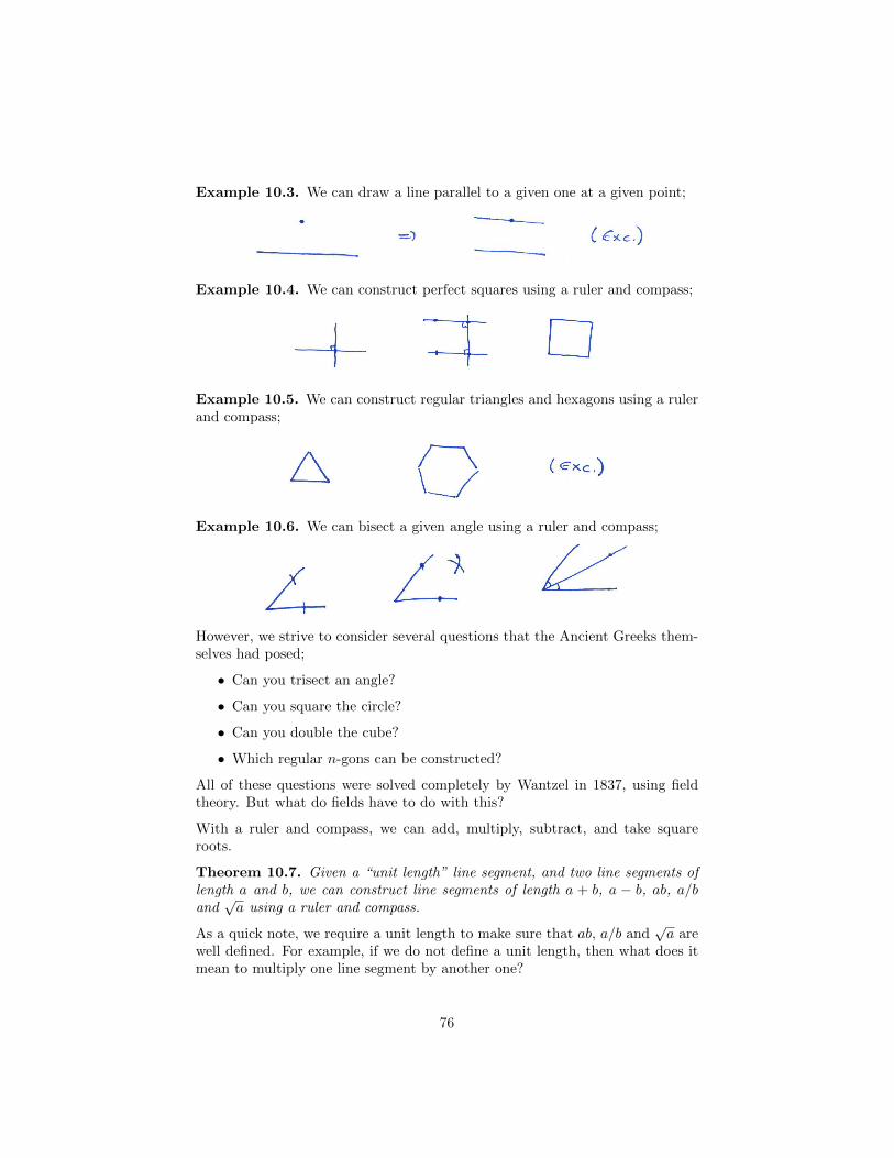
Example 10.3. We can draw a line parallel to a given one at a given point;

Example 10.4. We can construct perfect squares using a ruler and compass;

Example 10.5. We can construct regular triangles and hexagons using a rulerand compass;

Example 10.6. We can bisect a given angle using a ruler and compass;

However, we strive to consider several questions that the Ancient Greeks them-selves had posed;

• Can you trisect an angle?

• Can you square the circle?

• Can you double the cube?

• Which regular n-gons can be constructed?

All of these questions were solved completely by Wantzel in 1837, using fieldtheory. But what do fields have to do with this?

With a ruler and compass, we can add, multiply, subtract, and take squareroots.

Theorem 10.7. Given a “unit length” line segment, and two line segments oflength a and b, we can construct line segments of length a + b, a − b, ab, a/band√a using a ruler and compass.

As a quick note, we require a unit length to make sure that ab, a/b and√a are

well defined. For example, if we do not define a unit length, then what does itmean to multiply one line segment by another one?

76

Remarkably, it turns out that this is all one can do!

First, we make the statement precise - start with a line segment P0P1, andnothing else.

Definition 10.8. A point R is constructible if there is a finite sequence ofpoints P0, P1,︸ ︷︷ ︸

given

P2, . . . , Pm = R such that each Pk with 2 ≤ k ≤ m is obtained

from S = {P0, . . . , Pk−1} in one of 3 ways;

i Pk = intersection point of 2 distinct straight lines, each joining two pointsin S.

ii Pk is the intersection point of a line, as in (i), and a circle with the centrebeing a point in S and radius being the distance between 2 points in S.

iii Pk is the intersection point of two distinct circles as in (ii).

If we declare P0P1 to have unit length, we say that a number a ∈ R≥0 isconstructible if there is a line segment of length a with constructible endpoints- and we call −a constructible as well.

77

Introducing a coordinate system with (0, 0) = P0 and (1, 0) = P1 and consider-ing parallel lines through R to the coordinate axes, see immediately that

R = (a, b) is a constructible point if and only if a and b are constructible numbers.

Theorem 10.9. The set C of constructible numbers is a field,

Q ⊂ C ⊂ R

and is closed under taking square roots of positive numbers;

a ∈ C, a > 0 =⇒√a ∈ C

Proof. We have already shown that C is closed under addition, subtraction,multiplication, division, and taking square roots, and 0, 1 ∈ C by definition.

Wantzel proven the converse;

Theorem 10.10. a ∈ R is constructible if and only if there is a sequence offields

Q = K0 ⊂ K1 ⊂ · · · ⊂ Km ⊂ R,

a ∈ Km, and such that all [Kn : Kn−1] are 1 or 2. In other words, eitherKn = Kn−1 or Kn = Kn−1(

√αn−1) for some αn−1 ∈ Kn−1, for n = 1, . . . ,m.

Proof. We have already showed the backwards direction, that such a are con-structible, in the previous theorem.

So we aim to prove the forward direction; that if a is constructible, then R =(a, 0) is constructible, so take a sequence of points

P0 = (0, 0), P1 = (1, 0), P2, . . . , Pm = R

as in the definition of a constructible point.

Say Pi = (ai, bi). Let

K0 = K1 = QKi = Ki−1(ai, bi) = Q(a2, b2, . . . , a, bi)

for i = 2, . . . ,m, where Q(a2, b2, . . . , a, bi) is the smallest subfield of R thatcontains the coodinates of P2, . . . , Pi.

We want to show that [Ki : Ki−1] = 1 or 2 for every i.

Consider the first case, that Pi = L1∩L2, where L1 is a line through Pj , Pk andL2 is a line through Pr, Ps, with j, k, r, s < i.

78

Then we have

L1 : y =bj − bkaj − ak

(x− aj) + bj

L2 : y =br − bsar − as

(x− ar) + br

which are linear equations of the form y = αx+ β, α, β ∈ Ki−1.

Solving for x gives us the solution ai ∈ Ki−1. Also, we have that bi ∈ Ki−1, so

Ki −Ki−1

and hence [Ki : Ki−1] = 1 in this case.

So we now consider a second case, where Pi = L∩C, where L is a line throughPj , Pk, and C is a circle centred at Pr, passing through Ps. We have that

L : y = αx+ β, with α, β ∈ Ki−1 as above;

C : (x− ar)2 + (y − br)2 = d; d = (as− ar)2 + (bs− br)2

Substituting the first into the second gives us a quadratic equation on x

γx2 + δx+ ε = 0

where γ, δ and ε are all elements of Ki−1.

This has roots in Ki = Ki−1(√δ2 − 4γε), so ai is an element of this K, and

bi = αai + β, from the equation for L, is in Ki as well.

The third case we consider is if Pi = C1 ∩ C2, two circles;

C1 : (x− aj)2 + (y − bj)2 = d1,

C2 : (x− ar)2 + (y − bs)2 = d2

and subtracting one from the other causes x2 and y2 to cancel, and so we getthe equation of a line L, which implies that pi ∈ L∩C1, which we have alreadydone by case (ii).

Example 10.11. Since square roots have been shown to be constructible, that

means we can construct numbers such as√

2,√

3,√√

2 +√

3, and even√√√√32

11−√

3

13+√

7 +

√√√√7.

Example 10.12. We have that

cos2π

17=

1

β+√β

√√17 + 4

√17, β =

α+√

4 + α2

2, α =

1−√

17

2

79

and

sin2π

17=

√1− cos2

2π

17

are constructible, so that means we can construct a regular 17-gon.

Corollary 10.13. If α ∈ R is constructible, then [Q(α) : Q] = 2n for somen ≥ 0.

Proof. Q = K0 ⊂ K1 ⊂ . . . ⊂ Km implies that [Km : K0] is equal to somepower of 2.

Q = K0 ⊂ Q(α) ⊂ Km implies that [Q(α) : Q][Km : Q(α)] = [Km : Q], whichimplies that [Q(α) : Q] is a power of 2.

Corollary 10.14. Doubling the cube is impossible with a ruler and compass.

Proof. [Q( 3√

2) : Q] = 3, as the minimal polynomial of 3√

2 over Q is x3 − 2,which is monic and irreducible. Furthermore, as 3 is not a power of 2, then 3

√2

is not constructible.

Corollary 10.15. Squaring the circle is impossible with ruler and compass.

Proof. We have that√π is transcendental, so [Q(

√π) : Q] = ∞, and so

√π is

certainly not constructible.

Corollary 10.16. Trisecting the angle is impossible with ruler and compass.

Proof. Start with P0P1 and construct a regular triangle. If trisection were pos-sible, this angle of 2π

6 would be trisectable - in other words, we could constructthe angle 2π

18 and therefore cos(π9

), sin

(π9

). But the minimal polynomial of

α = cos(π9

)turns out to be

8x3 − 6x+ 1

which has no roots over Q and is hence irreducible, and so [Q(α) : Q] = 3.Therefore α is not constructible.

Similarly, not hard to deduce is that

Theorem 10.17. A regular n-gon is constructible with ruler and compass if andonly if n is a power of 2 multiplied by the product of distinct Fermat primes;

that is, primes of the form 22k

+ 1.

Proof. While not very hard, it is beyond the scope of this course, as it involvesa bit of Galois theory.

80

Example 10.18. Looking at Fermat primes, n = 3, 4, 5, 8, 10, 16, 17, . . . are allproducts of distinct Fermat primes, but not 7, 9, 11, 15.

The known Fermat primes are 3, 5, 17, 257, 65537.

The 65537-gon was constructed by J.G. Hermes in 1894, which took 200 pagesand 10 years to do. Wikipedia has an entry on this, if you are interested.

Often used notation

Z integersQ rational numbersR real numbersC complex numbersR, S ringsK, F fieldsR[x] polynomial ring in one variable, with coefficients in the ring RK(x) rational function field in one variable, with coefficients in a field K

its elements are quotients of two polynomials with coefficients in KR[α] when R ⊂ S and α ∈ S (as opposed to being an abstract symbol x

living nowhere, this is the smallest subring of S that contains R and αK(α) similarly, smallest field that contains K and αFq finite field with q elements, q a prime power. When q = p is a prime

number, this is just Z/pZ, the set of residue classes modulo pA ⊂ B same as A ⊆ B: “A is a subset of B, possibly equal to B”A ( B “A is a subset of B, not the whole of B”↪→ injective mapping� surjective mapping

Acknowledgements (TD). I would like to thank Jesse Parsons, Ross Bowden,Tom Schafer and Charlie Barker for corrections, and Yunzhu (Nancy) Mu fortaking notes of the revision lectures.

81