Embed Size (px)
Citation preview
Algebraic combinatorics for computational biology
by
Nicholas Karl Eriksson
B.S. (Massachusetts Institute of Technology) 2001
A dissertation submitted in partial satisfaction of the
requirements for the degree of
Doctor of Philosophy
in
Mathematics
and the Designated Emphasis
in
Computational and Genomic Biology
in the
GRADUATE DIVISION
of the
UNIVERSITY of CALIFORNIA, BERKELEY
Committee in charge:
Professor Bernd Sturmfels, ChairProfessor Lior Pachter
Professor Elchanan Mossel
Spring 2006

The dissertation of Nicholas Karl Eriksson is approved:
Chair Date
Date
Date
University of California, Berkeley
Spring 2006

Algebraic combinatorics for computational biology
Copyright 2006
by
Nicholas Karl Eriksson

1
Abstract
Algebraic combinatorics for computational biology
by
Nicholas Karl Eriksson
Doctor of Philosophy in Mathematics
University of California, Berkeley
Professor Bernd Sturmfels, Chair
Algebraic statistics is the study of the algebraic varieties that correspond to
discrete statistical models. Such statistical models are used throughout computational
biology, for example to describe the evolution of DNA sequences. This perspective on
statistics allows us to bring mathematical techniques to bear and also provides a source
of new problems in mathematics.
The central focus of this thesis is the use of the language of algebraic statistics
to translate between biological and statistical problems and algebraic and combinato-
rial mathematics. The wide range of biological and statistical problems addressed in
this work come from phylogenetics, comparative genomics, virology, and the analysis of
ranked data. While these problems are varied, the mathematical techniques used in this
work share common roots in the field of combinatorial commutative algebra. The main
mathematical theme is the use of ideals which correspond to combinatorial objects such
as magic squares, trees, or posets. Biological problems suggest new families of ideals,
and the study of these ideals can in some cases be useful for biology.
Professor Bernd SturmfelsDissertation Committee Chair

i
To Nirit
ii
Contents
List of Figures iv
List of Tables v
1 Introduction 1
1.1 Algebraic statistics . . . . . . . . . . . . . . . . . . . . . . . . . . . . . . . 21.2 Toric ideals and exponential families . . . . . . . . . . . . . . . . . . . . . 61.3 Phylogenetic algebraic geometry . . . . . . . . . . . . . . . . . . . . . . . 91.4 Genomics and phylogenetics . . . . . . . . . . . . . . . . . . . . . . . . . . 101.5 Outline of the thesis . . . . . . . . . . . . . . . . . . . . . . . . . . . . . . 13
2 Markov bases for noncommutative analysis of ranked data 15
2.1 Election data with five candidates . . . . . . . . . . . . . . . . . . . . . . 162.2 Fourier analysis of group valued data . . . . . . . . . . . . . . . . . . . . . 182.3 Exponential families . . . . . . . . . . . . . . . . . . . . . . . . . . . . . . 222.4 Computing Markov bases for permutation data . . . . . . . . . . . . . . . 242.5 Structure of the toric ideal ISn . . . . . . . . . . . . . . . . . . . . . . . . 262.6 Statistical analysis of the election data . . . . . . . . . . . . . . . . . . . . 302.7 Statistical analysis of an S4 example . . . . . . . . . . . . . . . . . . . . . 32
3 Toric ideals of homogeneous phylogenetic models 35
3.1 Homogeneous phylogenetic models . . . . . . . . . . . . . . . . . . . . . . 363.2 Toric ideals . . . . . . . . . . . . . . . . . . . . . . . . . . . . . . . . . . . 373.3 Viterbi polytopes . . . . . . . . . . . . . . . . . . . . . . . . . . . . . . . . 40
4 Tree construction using singular value decomposition 48
4.1 The general Markov model . . . . . . . . . . . . . . . . . . . . . . . . . . 494.2 Flattenings and rank conditions . . . . . . . . . . . . . . . . . . . . . . . . 494.3 Singular value decomposition . . . . . . . . . . . . . . . . . . . . . . . . . 544.4 Tree-construction algorithm . . . . . . . . . . . . . . . . . . . . . . . . . . 564.5 Building trees with simulated data . . . . . . . . . . . . . . . . . . . . . . 604.6 Building trees with real data . . . . . . . . . . . . . . . . . . . . . . . . . 61
iii
5 Ultra-conserved elements in vertebrate and fly genomes 65
5.1 The data . . . . . . . . . . . . . . . . . . . . . . . . . . . . . . . . . . . . 665.2 Ultra-conserved elements . . . . . . . . . . . . . . . . . . . . . . . . . . . . 69
5.2.1 Nine-vertebrate alignment . . . . . . . . . . . . . . . . . . . . . . . 705.2.2 ENCODE alignment . . . . . . . . . . . . . . . . . . . . . . . . . . 715.2.3 Eight-Drosophila alignment . . . . . . . . . . . . . . . . . . . . . . 72
5.3 Biology of ultra-conserved elements . . . . . . . . . . . . . . . . . . . . . . 735.3.1 Nine-vertebrate alignment . . . . . . . . . . . . . . . . . . . . . . . 735.3.2 ENCODE alignment . . . . . . . . . . . . . . . . . . . . . . . . . . 775.3.3 Eight-Drosophila alignment . . . . . . . . . . . . . . . . . . . . . . 785.3.4 Discussion . . . . . . . . . . . . . . . . . . . . . . . . . . . . . . . . 80
5.4 Statistical significance of ultra-conservation . . . . . . . . . . . . . . . . . 82
6 Evolution on distributive lattices 86
6.1 Drug resistance in HIV . . . . . . . . . . . . . . . . . . . . . . . . . . . . . 876.2 The model of evolution . . . . . . . . . . . . . . . . . . . . . . . . . . . . . 886.3 Fitness landscapes on distributive lattices . . . . . . . . . . . . . . . . . . 916.4 The risk of escape . . . . . . . . . . . . . . . . . . . . . . . . . . . . . . . 956.5 Distributive lattices from Bayesian networks . . . . . . . . . . . . . . . . . 996.6 Applications to HIV drug resistance . . . . . . . . . . . . . . . . . . . . . 1036.7 Mathematics and computation of the risk polynomial . . . . . . . . . . . . 1066.8 Discussion . . . . . . . . . . . . . . . . . . . . . . . . . . . . . . . . . . . . 112
Bibliography 115
iv
List of Figures
1.1 A simple statistical model. . . . . . . . . . . . . . . . . . . . . . . . . . . . 51.2 A multiple alignment of 3 DNA sequences. . . . . . . . . . . . . . . . . . . 12
2.1 Distribution of the projection to S3,2 for two random walks. . . . . . . . . 31
3.1 Polytope for a path with 7 nodes. . . . . . . . . . . . . . . . . . . . . . . . 423.2 The polytope of the completely odd binary tree. . . . . . . . . . . . . . . 453.3 A tree T with 15 nodes where PT has 34 vertices, 58 edges, and 26 facets. 46
4.1 Determining the rank of FlatA,B(P ) where {A,B} is not a split. . . . . . 524.2 The 6-taxa tree constructed in Example 4.16. . . . . . . . . . . . . . . . . 584.3 The eight-taxa tree used for simulations. . . . . . . . . . . . . . . . . . . . 604.4 Simulation results with branch lengths (a, b) = (0.01, 0.07). . . . . . . . . 614.5 Simulation results with branch lengths (a, b) = (0.02, 0.19). . . . . . . . . 624.6 Two phylogenetic trees for eight mammals. . . . . . . . . . . . . . . . . . 64
5.1 Phylogenetic tree for whole genome alignment of 9 vertebrates. . . . . . . 675.2 Phylogenetic tree for whole genome alignment of 8 Drosophila species. . . 685.3 Frequencies of vertebrate ultra-conserved elements (log10-scale). . . . . . . 705.4 Frequencies of Drosophila ultra-conserved elements (log10-scale). . . . . . 735.5 Functional base coverage of collapsed vertebrate ultra-conserved elements. 745.6 Ultra-conserved sequences found on either side of IRX5. . . . . . . . . . . 775.7 Functional base coverage of ultra-conserved elements in ENCODE regions. 785.8 Functional base coverage of ultra-conserved elements in Drosophila. . . . . 79
6.1 HIV protease enzyme with bound inhibitor. . . . . . . . . . . . . . . . . . 896.2 An event poset, its genotype lattice, and a fitness landscape. . . . . . . . 906.3 An event poset whose risk polynomial is of degree 11 in 375 unknowns. . . 986.4 Mutagenetic trees for ritonavir and indinavir. . . . . . . . . . . . . . . . . 1046.5 Graded resistance landscapes for ritonavir and indinavir. . . . . . . . . . . 1056.6 Risk as a function of drug dosage for indinavir and ritonavir. . . . . . . . 106
v
List of Tables
2.1 American Psychological Association ranked voting data. . . . . . . . . . . 172.2 First-order summary: chance of ranking candidate i in position j. . . . . . 182.3 A Markov basis for S5 with 29890 moves in 14 symmetry classes. . . . . . 192.4 Length of the data projections onto the 7 isotypic subspaces of S5. . . . . 202.5 Second order summary for the APA data. . . . . . . . . . . . . . . . . . . 212.6 Markov bases for S3 and S4 and the size of their symmetry classes. . . . . 252.7 Number of generators by degree in a Markov basis for Sn. . . . . . . . . . 272.8 Length of the data projections for the APA data and three perturbations. 302.9 S4 ranked data. . . . . . . . . . . . . . . . . . . . . . . . . . . . . . . . . . 332.10 First order summary for the S4 ranked data in Table 2.9. . . . . . . . . . 332.11 Length of the data projections for the S4 data and three perturbations. . 33
3.1 Generators of the toric ideals of binary trees. . . . . . . . . . . . . . . . . 393.2 Generators of the toric ideals of paths. . . . . . . . . . . . . . . . . . . . . 413.3 Statistics for the polytopes of binary trees with at most 23 nodes. . . . . . 463.4 Statistics for the polytopes of all trees with at most 15 nodes. . . . . . . . 47
4.1 Comparison of the SVD algorithm and dnaml on ENCODE data. . . . . . 63
5.1 Example of the output of Mercator. . . . . . . . . . . . . . . . . . . . . . 665.2 Genomes in the nine-vertebrate alignment. . . . . . . . . . . . . . . . . . . 675.3 Genomes in the eight-Drosophila alignment. . . . . . . . . . . . . . . . . . 685.4 Ultra-conserved elements in the ENCODE alignments. . . . . . . . . . . . 725.5 GO annotations of genes associated with vertebrate ultras. . . . . . . . . 765.6 ENCODE regions with the greatest number of ultra-conserved elements. . 795.7 GO annotations of genes associated with Drosophila ultras. . . . . . . . . 815.8 Probability of seeing ultra-conserved elements in an independence model. 84

vi
Acknowledgements
Above all, thanks to my advisor, Bernd Sturmfels, from whom I have learned much about
the mysterious processes of doing and communicating mathematics. As essentially my
second advisor, Lior Pachter has been an excellent guide through the rugged terrain that
lies between mathematics and computational biology.
I would not be in this position without a host of mentors and teachers, partic-
ularly Jim Cusker and Ken Ono, who started me on this path of studying mathematics.
Along the way, it has been a pleasure to learn from my amazing coauthors: Niko Beeren-
winkel, Persi Diaconis, Mathias Drton, Steve Fienberg, Jeff Lagarias, Garmay Leung,
Kristian Ranestad, Alessandro Rinaldo, Seth Sullivant, and Bernd Sturmfels.
I am grateful for support from the National Science Foundation (grant EF-
0331494), the DARPA program Fundamental Laws in Biology (HR0011-05-1-0057), and
a National Defense Science and Engineering Graduate Fellowship. Due to this support
and support from my advisors, I have had the good fortune to travel the world learning
and teaching mathematics. From Palo Alto to Spain to Argentina and many places in
between, the people I have met on these trips have enriched my mathematical life.
As this thesis depends heavily on computation, I am indebted to the people
who have written programs which proved invaluable for my research. In particular, I
thank Raymond Hemmecke, whose program 4ti2 was vital for Chapters 2 and 3. Also,
thanks to Susan Holmes and Aaron Staple for writing the R code used in Chapter 2.
Most importantly, my parents, sister, and wife are each more responsible for
my successes than they or I usually realize. They have always supported, accepted, and
nourished me in countless ordinary and extraordinary ways.

1
Chapter 1
Introduction
The main theme of this thesis is the interplay between statistical models and
algebraic techniques. More and more, the fields of statistics and biology are generating a
wealth of interesting mathematical questions. In return, discrete mathematics provides
techniques for the solution of these problems, as well as a theoretical framework from
which to ask new questions. From this interplay, the field of algebraic statistics has
emerged. Its main purpose is the development of computational and theoretical tech-
niques in algebra and combinatorics for applications to practical statistical problems.
These techniques supply a valuable mathematical language for the study of computa-
tional biology.
Computational biology has been a wonderful source of problems in combina-
torics and combinatorial computer science due to the discrete structure of biological
objects, notably DNA. For example, counting alignments and counting RNA secondary
structures are typical enumerative problems [104]. For other connections between the
fields, we note how biology has motivated mathematicians to better understand the struc-
ture of the space of trees [16] and how distance measures between signed permutations
[41] provide methods for understanding genome rearrangement through evolution.
While biology provides a fount of such interesting questions, it is desirable at
the end of the day to better understand real data. And because there is always error
in experimental data, this problem requires the use of statistics. Thus, we must form a
connection between statistics and mathematics that allows us to use the combinatorial

2
properties of the underlying problems in order to analyze data in a rigorous, robust, and
efficient way.
In this thesis, we provide a series of interrelated illustrations of how algebraic
combinatorics can be used to increase our understanding of statistical and biological
problems. We also demonstrate how biological questions can lead to interesting math-
ematics. The examples we study are drawn from statistics, phylogenetics, comparative
genomics, and virology. The underlying mathematical philosophy is that statistical mod-
els can be viewed as algebraic varieties. Our examples draw from a small set of statistical
models which we introduce in this chapter: exponential families, phylogenetic models,
and Bayesian networks.
In the rest of this introduction, we will briefly outline the new field of algebraic
statistics and explain the major algebraic, statistical, and biological ideas that will be
used throughout the thesis. We refer the reader to the book [73] for more details.
1.1 Algebraic statistics
Algebraic statistics depends on a set of tools that allow us to translate problems in statis-
tics into algebraic language. We assume the reader is familiar with the basic language of
algebraic geometry, namely polynomials, ideals, and varieties. In addition, we will use
Grobner bases throughout the thesis as a computational tool. For a friendly introduction
to ideals and Grobner bases, see [27].
Let X be a discrete random variable taking values in the set [n] = {1, 2, . . . , n}.
We write pi as shorthand for Pr(X = i), the probability that X is in state i. Let ∆n−1
be the (n − 1) dimensional probability simplex, e.g.,
∆n−1 = {(p1, . . . , pn) ∈ Rn | pi ≥ 0,
n∑
i=1
pi = 1}.
We will write ∆ for the simplex ∆n−1 when the space is understood. A statistical
model for X is simply a family of probability distributions M ⊂ ∆. We will restrict
our attention to statistical models M which are given as the image of a polynomial
parameterization. That is, for every vector of parameters θ = (θ1, . . . , θd) we associate
a probability distribution (p1(θ), . . . , pn(θ)) ∈ ∆ where p1(θ), . . . , pn(θ) are polynomials
3
in d unknowns. Given such a polynomial map
p : Rd → R
n
θ = (θ1, . . . , θd) 7→ (p1(θ), p2(θ), . . . , pn(θ)),
the associated statistical model is given by M = p(Θ) where Θ is an appropriate, non-
empty, open set in Rd, called the parameter space. If we are concerned with obtaining
actual probability distributions via this map, we can either impose constraints on Θ in
order to make sure that p(Θ) ⊂ ∆, or we can take the model to be M = p(Θ) ∩ ∆.
However, we shall usually ignore this issue and will even assume that the ground field is
C rather than R in order to work over an algebraically closed field.
A natural question we might ask about a statistical model is what relations
among the probabilities p1, . . . , pn are satisfied at all points in the model p. Since p is
a polynomial map, these relations are given by polynomials which can be found using
Grobner bases.
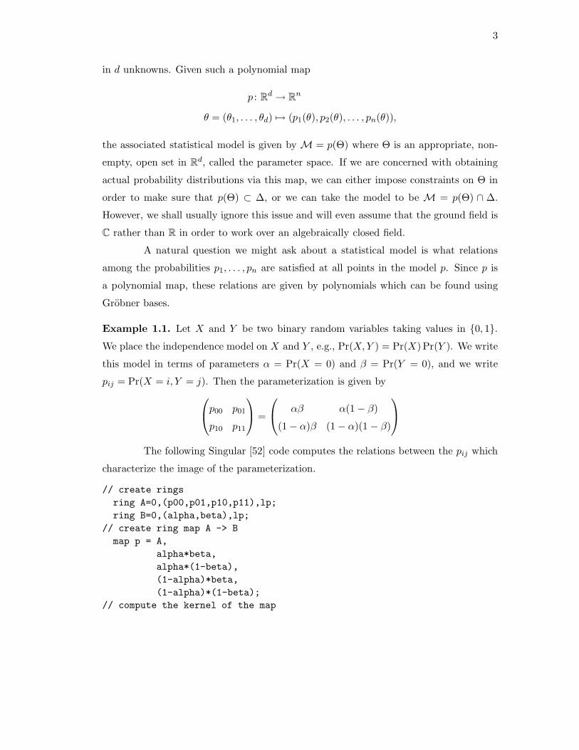
Example 1.1. Let X and Y be two binary random variables taking values in {0, 1}.
We place the independence model on X and Y , e.g., Pr(X,Y ) = Pr(X) Pr(Y ). We write
this model in terms of parameters α = Pr(X = 0) and β = Pr(Y = 0), and we write
pij = Pr(X = i, Y = j). Then the parameterization is given by
p00 p01
p10 p11
=
αβ α(1 − β)
(1 − α)β (1 − α)(1 − β)
The following Singular [52] code computes the relations between the pij which
characterize the image of the parameterization.
// create rings
ring A=0,(p00,p01,p10,p11),lp;
ring B=0,(alpha,beta),lp;
// create ring map A -> B
map p = A,
alpha*beta,
alpha*(1-beta),
(1-alpha)*beta,
(1-alpha)*(1-beta);
// compute the kernel of the map
4
ideal B0 = 0;
setring A;
preimage(B,p,B0);
Singular outputs the following:
_[1]=p01*p10+p01*p11+p10*p11+p11^2-p11
_[2]=p00+p01+p10+p11-1
The second polynomial is the condition that the probabilities sum to one. The first
polynomial doesn’t look familiar, but after substituting p11 = 1 − p00 − p01 − p10 for
one of the factors p11 in the term p211, we get the determinant of the joint probability
matrix p00p11 − p01p10 as expected. We actually did not need to make this polynomial
homogeneous by hand, we could have made the map homogeneous instead and then
added in the condition that the probabilities sum to one. Statisticians might recognize
this determinant as the odds ratio p00p11
p01p10= 1 in the case where all probabilities are
non-zero.
Next we give a slightly less trivial example which is a special case of two impor-
tant classes of statistical models studied in this thesis: phylogenetic models and Bayesian
networks.
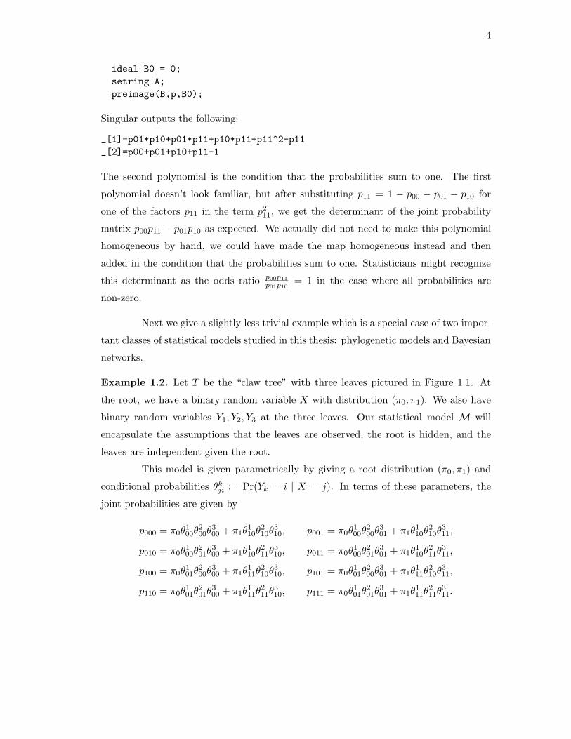
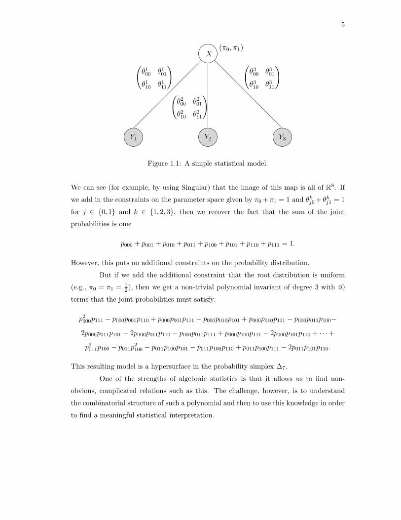
Example 1.2. Let T be the “claw tree” with three leaves pictured in Figure 1.1. At
the root, we have a binary random variable X with distribution (π0, π1). We also have
binary random variables Y1, Y2, Y3 at the three leaves. Our statistical model M will
encapsulate the assumptions that the leaves are observed, the root is hidden, and the
leaves are independent given the root.
This model is given parametrically by giving a root distribution (π0, π1) and
conditional probabilities θkji := Pr(Yk = i | X = j). In terms of these parameters, the
joint probabilities are given by
p000 = π0θ100θ
200θ
300 + π1θ
110θ
210θ
310, p001 = π0θ
100θ
200θ
301 + π1θ
110θ
210θ
311,
p010 = π0θ100θ
201θ
300 + π1θ
110θ
211θ
310, p011 = π0θ
100θ
201θ
301 + π1θ
110θ
211θ
311,
p100 = π0θ101θ
200θ
300 + π1θ
111θ
210θ
310, p101 = π0θ
101θ
200θ
301 + π1θ
111θ
210θ
311,
p110 = π0θ101θ
201θ
300 + π1θ
111θ
211θ
310, p111 = π0θ
101θ
201θ
301 + π1θ
111θ
211θ
311.
5
(
θ200 θ2
01
θ210 θ2
11
)
(
θ100 θ1
01
θ110 θ1
11
) (
θ300 θ3
01
θ310 θ3
11
)
(π0, π1)
Y2Y1 Y3
X
Figure 1.1: A simple statistical model.
We can see (for example, by using Singular) that the image of this map is all of R8. If
we add in the constraints on the parameter space given by π0 + π1 = 1 and θkj0 + θk
j1 = 1
for j ∈ {0, 1} and k ∈ {1, 2, 3}, then we recover the fact that the sum of the joint
probabilities is one:
p000 + p001 + p010 + p011 + p100 + p101 + p110 + p111 = 1.
However, this puts no additional constraints on the probability distribution.
But if we add the additional constraint that the root distribution is uniform
(e.g., π0 = π1 = 12), then we get a non-trivial polynomial invariant of degree 3 with 40
terms that the joint probabilities must satisfy:
p2000p111 − p000p001p110 + p000p001p111 − p000p010p101 + p000p010p111 − p000p011p100−
2p000p011p101 − 2p000p011p110 − p000p011p111 + p000p100p111 − 2p000p101p110 + · · ·+
p2011p100 − p011p
2100 − p011p100p101 − p011p100p110 + p011p100p111 − 2p011p101p110.
This resulting model is a hypersurface in the probability simplex ∆7.
One of the strengths of algebraic statistics is that it allows us to find non-
obvious, complicated relations such as this. The challenge, however, is to understand
the combinatorial structure of such a polynomial and then to use this knowledge in order
to find a meaningful statistical interpretation.

6
This model is called a naive Bayes model. It is a special case of the phylo-
genetic models that we will introduce in Section 1.3 and study in Chapters 3, 4, and
5. Phylogenetic models are special cases of Bayesian networks, which will be used in
Chapter 6.
1.2 Toric ideals and exponential families
An important special class of polynomial ideals are the toric ideals. Toric ideals are prime
ideals with a generating set of binomials. Equivalently, they are given by a monomial
parameterization. In this section, we provide a brief introduction to the theory of toric
ideals and their close relationship to the statistical models called exponential families.
See [98] for more details about toric ideals.
Let A be a d×n matrix with integer entries written as A = (aij) = (a1, . . . ,an) ∈
Zd×n. This matrix determines a map, fA : (C∗)d → C
n, given by
fA(θ1, . . . , θd) =
(
d∏
i=1
θai1i ,
d∏
i=1
θai2i , . . . ,
d∏
i=1
θain
i
)
Definition 1.3. The toric variety XA is the closure of the image of the map fA. If
every column of A has the same sum, we say that A is homogeneous and that XA is a
projective toric variety.
Definition 1.4. The toric ideal IA ⊂ C[p] is the vanishing ideal of XA. Alternatively,
we can define IA via the (infinite) generating set
IA = 〈pu − pv | A(u− v) = 0 and u,v ∈ Zn≥0〉.
If A is homogeneous, then the binomials pu − pv are homogeneous.
Projective toric varieties correspond to an important subclass of exponential
families, the log-linear models.
Definition 1.5. The log-linear model MA associated to A = (a1, . . . ,an) is the proba-
bility distribution in ∆n−1 defined by
Pθ(X = i) =1
Ze〈ai,θ〉 for 1 ≤ i ≤ n, θ ∈ R
d.
7
where Z =∑n
i=1 e〈ai,θ〉 is a normalizing constant and 〈, 〉 is the standard inner product
on Rn.
To see that IA vanishes on MA, notice that for u = (u1, . . . , un) ∈ Nn with
∑ni=1 ui = N ,
pu =
n∏
i=1
Pθ(X = i)ui =1
ZNe
Pni=1 ui〈ai,θ〉 =
1
ZNe〈Au,θ〉.
Therefore, if Au = Av and A is homogeneous, we see that pu−pv vanishes on the model
MA. Notice that if we remove the normalizing factor Z−1 in the definition of a log-linear
model this corresponds to switching to the affine toric variety from the projective one.
Now suppose that we have a series of observations X1, . . . ,XN ∈ [n] that are
independent draws from the distribution given by some unknown probability vector p
in the model M. For statistical inference about p using the likelihood framework we
work with the likelihood function which associates to every p ∈ M the probability of
observing X1, . . . ,XN given the distribution p. This likelihood clearly depends only on
the counts u ∈ Zn, where ui is the number of X1, . . . ,XN that equal i. As we saw above,
the probability of observing X1, . . . ,XN is given by
Pθ(X1, . . . ,XN ) =
1
ZNe〈Au,θ〉.
That is, Au is a sufficient statistic for the model Pθ.
We can consider Pθ as a distribution on the counts u by
Pθ(u) =
(
N
u1, . . . , un
)
1
ZNe〈Au,θ〉.
This corresponds to forgetting the order of the samples X1, . . . ,XN . An elementary
calculation shows that
Pθ(u | Au = t)
does not depend on θ, this is true precisely because A is a sufficient statistic. This
property will prove important in Chapter 2 when we wish to sample from the conditional
distribution of all data with a fixed sufficient statistic.
We conclude our discussion of toric ideals with a description of how to compute
generators for toric ideals using the software 4ti2 [53].

8
Example 1.6. Let T again be the claw tree with three leaves. We take the same model
as in Example 1.2 except we make the root node observed and we require that each
edge has the same transition matrix. This is called the the fully observed, homogeneous,
binary Markov model on T and will be studied in Chapter 3.
Take the root distribution to be uniform and relax the condition that the tran-
sition parameters sum to one. This leaves four parameters which we write θ00, θ01, θ10,
and θ11. This is a toric model, since the parameterization pijkl = θijθikθil is monomial
(we write pijkl for the probability that the root is in state i and the leaves are in states
j, k, and l). This parameterization corresponds to a 4 × 16 matrix A which we save in
a file tree3 in the form
4 16
3 2 2 1 2 1 1 0 0 0 0 0 0 0 0 0
0 1 1 2 1 2 2 3 0 0 0 0 0 0 0 0
0 0 0 0 0 0 0 0 3 2 2 1 2 1 1 0
0 0 0 0 0 0 0 0 0 1 1 2 1 2 2 3
For example, column three of A corresponds to the probability p0010 = θ200θ01 of having
a tree with a zero at the root and at two of the three leaves. To find a Grobner basis,
run the command groebner tree3 which produces an output file named tree3.gro
14 16
-1 1 0 1 0 0 0 -1 0 0 0 0 0 0 0 0
-1 2 0 -1 0 0 0 0 0 0 0 0 0 0 0 0
0 -1 0 0 1 0 0 0 0 0 0 0 0 0 0 0
0 -1 0 2 0 0 0 -1 0 0 0 0 0 0 0 0
0 -1 1 0 0 0 0 0 0 0 0 0 0 0 0 0
0 0 0 -1 0 0 1 0 0 0 0 0 0 0 0 0
0 0 0 -1 0 1 0 0 0 0 0 0 0 0 0 0
0 0 0 0 0 0 0 0 -1 1 0 1 0 0 0 -1
0 0 0 0 0 0 0 0 -1 2 0 -1 0 0 0 0
0 0 0 0 0 0 0 0 0 -1 0 0 1 0 0 0
0 0 0 0 0 0 0 0 0 -1 0 2 0 0 0 -1
0 0 0 0 0 0 0 0 0 -1 1 0 0 0 0 0
0 0 0 0 0 0 0 0 0 0 0 -1 0 0 1 0
0 0 0 0 0 0 0 0 0 0 0 -1 0 1 0 0
Each row w of this matrix corresponds to an element of the Grobner basis as follows.
Write w in the form u− v where u,v ∈ N16. Then the row corresponds to the binomial
9
pu − pv. For example, row two gives the relation p20001 − p0000p0011.
Notice that of the fourteen basis elements, eight are linear (e.g., row three) and
six are of degree two (e.g., row one). Modulo the linear relations, algebraic geometers will
recognize this variety as being the free join of two copies of the third Veronese embedding
of P1 in P
3.
1.3 Phylogenetic algebraic geometry
In this section, we introduce Markov models on trees, a subject that will be explored
further in Chapters 3, 4, and 5. As above, a statistical model on a tree gives an algebraic
variety, and these varieties depend in interesting ways on the combinatorics of the trees
and of the underlying statistical model. For more details on the algebraic viewpoint on
phylogenetics, with many references and open problems, see [45].
The basic object in a phylogenetic model is a tree T which is rooted and has n
labeled leaves. Each node of the tree T is a random variable taking values in the alphabet
Σ. We write k = |Σ| for the number of possible states. At the root, the distribution of the
states is given by π = (π1, . . . , πk). On each edge e of the tree there is a k × k transition
matrix Me whose entries are indeterminates representing the probabilities of transition
(away from the root) between the states. Typically, the random variables at the interior
nodes will be hidden and the random variables at the leaves will be observed, although
we will also consider the case where all nodes are observed in Chapter 3. The entries
of the matrices Me and the vector π are the model parameters. For instance, if T is a
binary tree with n leaves then T has 2n− 2 edges, and hence we have d = (2n− 2)k2 + k
parameters.
In practice, there will be many constraints on these parameters, usually express-
ible in terms of linear equations and inequalities, so the set of statistically meaningful
parameters is a polyhedron Θ in Rd. For example, one common set of constraints corre-
sponds to making the rows of the transition matrices Me and the vector π sum to one.
Specifying this subset Θ means choosing a model of evolution. In the next section we
will discuss several models of evolution with different degrees of biological relevance.
At each leaf of T we can observe k possible states, so there are kn possible
10
joint observations we can make at the leaves. The probability pσ of making a particular
observation σ ∈ Σn is a polynomial in the model parameters. Hence we get a polynomial
map whose coordinates are the polynomials pσ,
p : Θ ⊂ Rd → R
kn
(θ1, . . . , θd) 7→ (pσ(θ) | σ ∈ Σn).
The image of this map is our phylogenetic model.
For every tree and every parameter set Θ, we get such a variety. This leads to
a host of interesting algebraic questions. For example: pick Θ and describe the resulting
stratification of Rkn
by the varieties for all trees with n leaves.
Example 1.7. Again, let T be the claw tree with three leaves in Figure 1.1. As in
Example 1.2 make the root node hidden, and let all the random variables have k states.
We fix no constraints on the parameters, so each edge has k2 parameters associated to
it. This model is called the general Markov model. The variety of T is given by
XT = Seck(Pk−1 × Pk−1 × P
k−1),
where we write Seck(V ) for the k-th secant variety of V (i.e., the variety of all secant
Pk−1’s to V ). To see this, notice that the parameterization consists of one copy of the
parameterization of the Segre variety for each value of the hidden state. We have seen this
parameterization for k = 2 in Example 1.2, where we saw that Sec2(P1 × P1 × P
1) = P7.
1.4 Genomics and phylogenetics
Phylogenetics is the field of biology concerned with resolving the evolutionary relation-
ships among and between organisms. With the recent explosion of genomic data, the
focus of phylogenetics has been on understanding models of DNA evolution and us-
ing these models to infer ancestral relationships. Standard phylogenetic techniques fall
broadly into two classes: distance based and character based. Distance methods rely on
estimating pairwise distances between species and then try to find a tree which gives
similar distances. The most common example of this method is neighbor joining [83].
Character based methods start with a multiple alignment (defined below) and typically
11
perform model selection in some family of statistical models of evolution. For example,
likelihood or parsimony methods are character based. We believe that algebraic statistics
provides an interesting new viewpoint on character based tree construction techniques.
In this section, we describe some of the basic biological facts needed to un-
derstand phylogenetic models and then delve into the practical side of the algebraic
statistics of these models. See the books [46, 86] for introductions to the mathematical
and algorithmic sides of the field of phylogenetics.
The basic genetic information of an organism is (almost always) carried in the
form of DNA, a double helix consisting of two complementary polymers bound together.
The four nucleotides that form DNA come in two types: the purines (A and G) and the
pyrimidines (C and T). The two strands of the double helix are joined together via the
base pairings A to T (via 2 hydrogen bonds) and C to G (via 3 hydrogen bonds).
Since each cell typically contains a copy of the DNA of the organism, DNA
copying occurs frequently. Several types of errors are possible during the replication
of DNA. Single bases can mutate, or large pieces of DNA can separate and become
reattached, possibly at another position, possibly in the opposite direction. These are
just some of the events that occur over the course of evolution.
In order to understand the relationships of various species from DNA data, we
must find sections of DNA in each species which we believe share a common ancestor.
This problem is called orthology mapping, and can be solved using software such as
mercator [32]. After orthologous regions are identified, they must be aligned using a
program such as MAVID [18]. The starting point for phylogenetic algorithms is a multiple
sequence alignment, as pictured in Figure 1.2. We will write an alignment as a set of n
strings of equal length from the alphabet Σ. In Figure 1.2, Σ = {A, C, G, T, -}.
The standard assumption in character-based phylogenetics is that evolution
happens independently at each point in the genome. We explore this assumption in
Chapter 5, searching for parts of the genome with extreme and unexpected correlation
between adjacent sites. However, the independence assumption makes the problem of
phylogenetics much easier since then the columns of the alignment can be considered as
independent, identically distributed samples.
In this manner, an alignment of n species gives an observed probability dis-
12
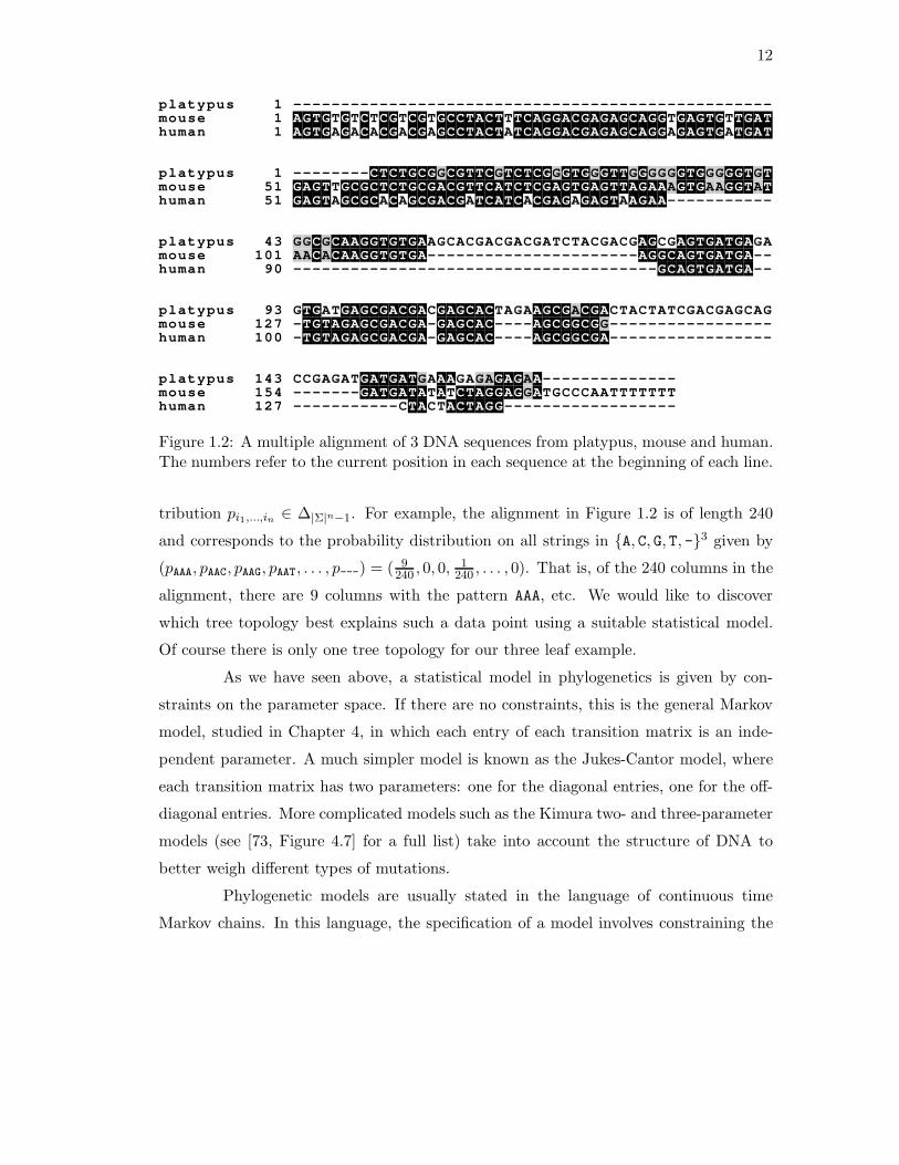
platypus 1 --------------------------------------------------mouse 1 AGTGTGTCTCGTCGTGCCTACTTTCAGGACGAGAGCAGGTGAGTGTTGAThuman 1 AGTGAGACACGACGAGCCTACTATCAGGACGAGAGCAGGAGAGTGATGAT
platypus 1 --------CTCTGCGGCGTTCGTCTCGGGTGGGTTGGGGGGTGGGGGTGTmouse 51 GAGTTGCGCTCTGCGACGTTCATCTCGAGTGAGTTAGAAAGTGAAGGTAThuman 51 GAGTAGCGCACAGCGACGATCATCACGAGAGAGTAAGAA-----------
platypus 43 GGCGCAAGGTGTGAAGCACGACGACGATCTACGACGAGCGAGTGATGAGAmouse 101 AACACAAGGTGTGA----------------------AGGCAGTGATGA--human 90 --------------------------------------GCAGTGATGA--
platypus 93 GTGATGAGCGACGACGAGCACTAGAAGCGACGACTACTATCGACGAGCAGmouse 127 -TGTAGAGCGACGA-GAGCAC----AGCGGCGG-----------------human 100 -TGTAGAGCGACGA-GAGCAC----AGCGGCGA-----------------
platypus 143 CCGAGATGATGATGAAAGAGAGAGAA--------------mouse 154 -------GATGATATATCTAGGAGGATGCCCAATTTTTTThuman 127 -----------CTACTACTAGG------------------
Figure 1.2: A multiple alignment of 3 DNA sequences from platypus, mouse and human.The numbers refer to the current position in each sequence at the beginning of each line.
tribution pi1,...,in ∈ ∆|Σ|n−1. For example, the alignment in Figure 1.2 is of length 240
and corresponds to the probability distribution on all strings in {A, C, G, T, -}3 given by
(pAAA, pAAC, pAAG, pAAT, . . . , p---) = ( 9240 , 0, 0, 1
240 , . . . , 0). That is, of the 240 columns in the
alignment, there are 9 columns with the pattern AAA, etc. We would like to discover
which tree topology best explains such a data point using a suitable statistical model.
Of course there is only one tree topology for our three leaf example.
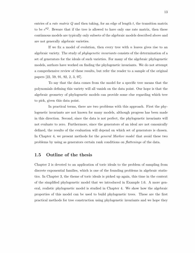
As we have seen above, a statistical model in phylogenetics is given by con-
straints on the parameter space. If there are no constraints, this is the general Markov
model, studied in Chapter 4, in which each entry of each transition matrix is an inde-
pendent parameter. A much simpler model is known as the Jukes-Cantor model, where
each transition matrix has two parameters: one for the diagonal entries, one for the off-
diagonal entries. More complicated models such as the Kimura two- and three-parameter
models (see [73, Figure 4.7] for a full list) take into account the structure of DNA to
better weigh different types of mutations.
Phylogenetic models are usually stated in the language of continuous time
Markov chains. In this language, the specification of a model involves constraining the
13
entries of a rate matrix Q and then taking, for an edge of length t, the transition matrix
to be etQ. Beware that if the tree is allowed to have only one rate matrix, then these
continuous models are typically only subsets of the algebraic models described above and
are not generally algebraic varieties.
If we fix a model of evolution, then every tree with n leaves gives rise to an
algebraic variety. The study of phylogenetic invariants consists of the determination of a
set of generators for the ideals of such varieties. For many of the algebraic phylogenetic
models, authors have worked on finding the phylogenetic invariants. We do not attempt
a comprehensive review of these results, but refer the reader to a sample of the original
papers [22, 59, 91, 92, 2, 3, 97].
To say that the data comes from the model for a specific tree means that the
polynomials defining this variety will all vanish on the data point. Our hope is that the
algebraic geometry of phylogenetic models can provide some clue regarding which tree
to pick, given this data point.
In practical terms, there are two problems with this approach. First the phy-
logenetic invariants are not known for many models, although progress has been made
in this direction. Second, since the data is not perfect, the phylogenetic invariants will
not evaluate to zero. Furthermore, since the generators of an ideal are not canonically
defined, the results of the evaluation will depend on which set of generators is chosen.
In Chapter 4, we present methods for the general Markov model that avoid these two
problems by using as generators certain rank conditions on flattenings of the data.
1.5 Outline of the thesis
Chapter 2 is devoted to an application of toric ideals to the problem of sampling from
discrete exponential families, which is one of the founding problems in algebraic statis-
tics. In Chapter 3, the theme of toric ideals is picked up again, this time in the context
of the simplified phylogenetic model that we introduced in Example 1.6. A more gen-
eral, realistic phylogenetic model is studied in Chapter 4. We show how the algebraic
properties of this model can be used to build phylogenetic trees. These are the first
practical methods for tree construction using phylogenetic invariants and we hope they

14
can provide motivation for how algebraic statistics can be used in practice.
In Chapter 5, we study genomic sequences which are perfectly preserved at
extreme evolutionary distances. This provides an example of how comparative genomics
can help derive the function of genomic elements. We also apply our phylogenetic models
to quantify the evolutionary significance of these highly-conserved elements. Finally, in
Chapter 6 we again study evolution, but this time in the very specialized case in which
the organism is under severe pressure and can evolve in only one direction. The set of
possible genotypes is modeled as a distributive lattice and Bayesian networks are used
to study evolution proceeding up this lattice. We are concerned with the risk that the
organism escapes from the selective pressure, which is the probability that it evolves to
the top of the lattice before becoming extinct. This risk depends on the combinatorics
of the lattice.
15
Chapter 2
Markov bases for noncommutative
analysis of ranked data
In this chapter, we give a general methodology for studying group valued data
where the summary we are interested in is given by a representation of the group. In
particular, we analyze in detail the case of ranked data. Our main example of ranked
data is the case of an election where every voter was asked to rank the five candidates.
Our methods depend on two tools. First, we show how Fourier analysis and
representation theory can be used to obtain descriptive statistics of group-valued data.
In the case of ranked data, this gives in particular a description of how likely a voter
would be to rank a given pair of candidates in a given pair of positions. Second, in order
to calibrate these methods, we show how to use Markov chain Monte Carlo techniques to
sample from group-valued data with a fixed summary. In order to run a Markov chain, a
set of moves (a Markov basis) is needed. We calculate this basis using the theory of toric
ideals and show how symmetry can be very helpful in these calculations. The material
in this chapter comes from the paper [37], with Persi Diaconis.
We believe that these methods can be useful in computational biology. For
example, suppose we want to understand how the fitness of an organism depends on
the order of certain genes in its genome. Understanding this dependence can lead to a
picture of the regulatory network for these genes. The function that assigns a fitness
value to each ordering of the genes is called a fitness landscape. This fitness landscape

16
can be analyzed using the methods discussed in this chapter in order to understand how
the position of a pair of genes affects the total fitness.
From the perspective of [11], a fitness landscape corresponds to a triangulation
of a certain polytope that encodes the space of genotypes. In our case, this polytope
is the Birkhoff polytope. It would be interesting to study the relationship between the
triangulations of the Birkhoff polytope obtained from fitness landscapes and the spectral
analysis presented in this chapter.
2.1 Election data with five candidates
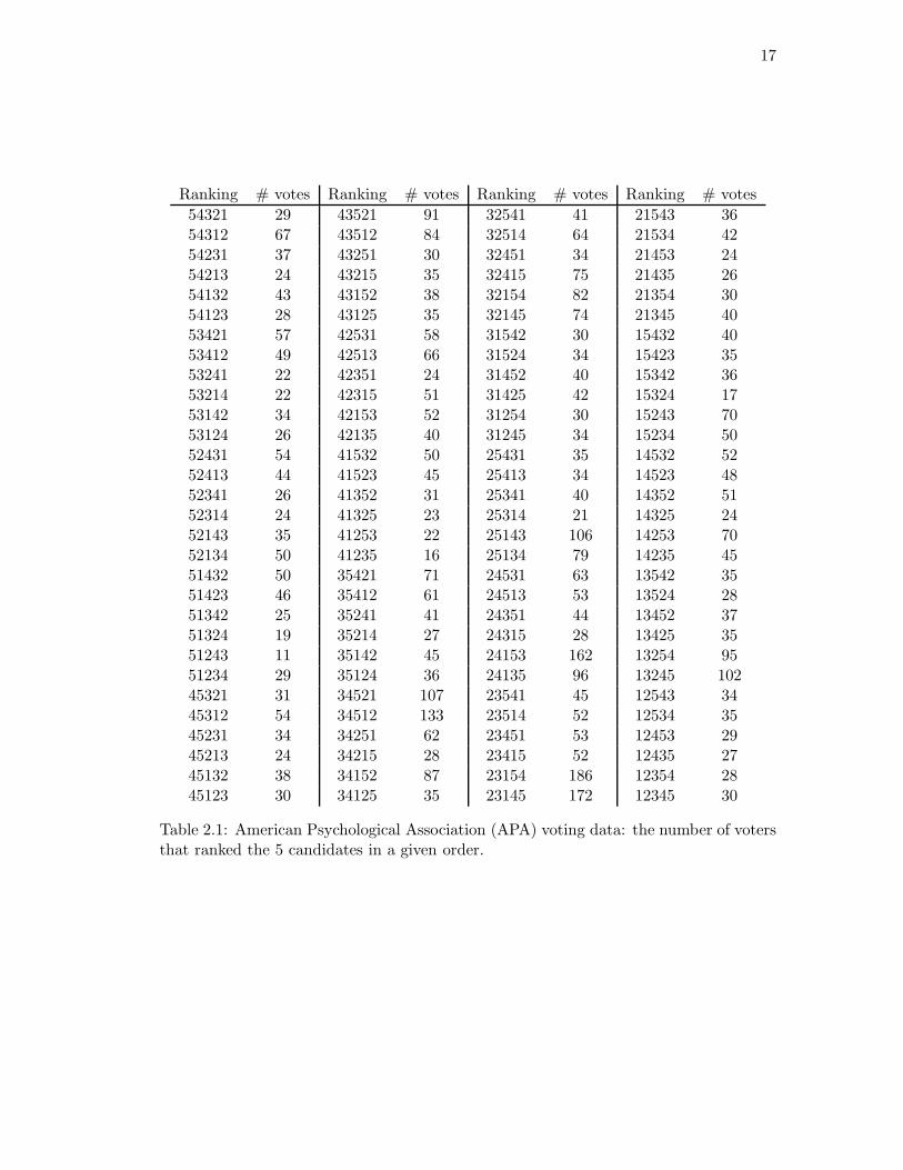
Table 2.1 shows the results of an election. A population of 5738 voters was asked to rank
five candidates for president of a national professional organization. The table shows the
number of voters choosing each ranking. For example, 29 voters ranked candidate 5 first,
candidate 4 second, . . . , and candidate 1 last, resulting in the entry 54321 = 29. Table 2.2
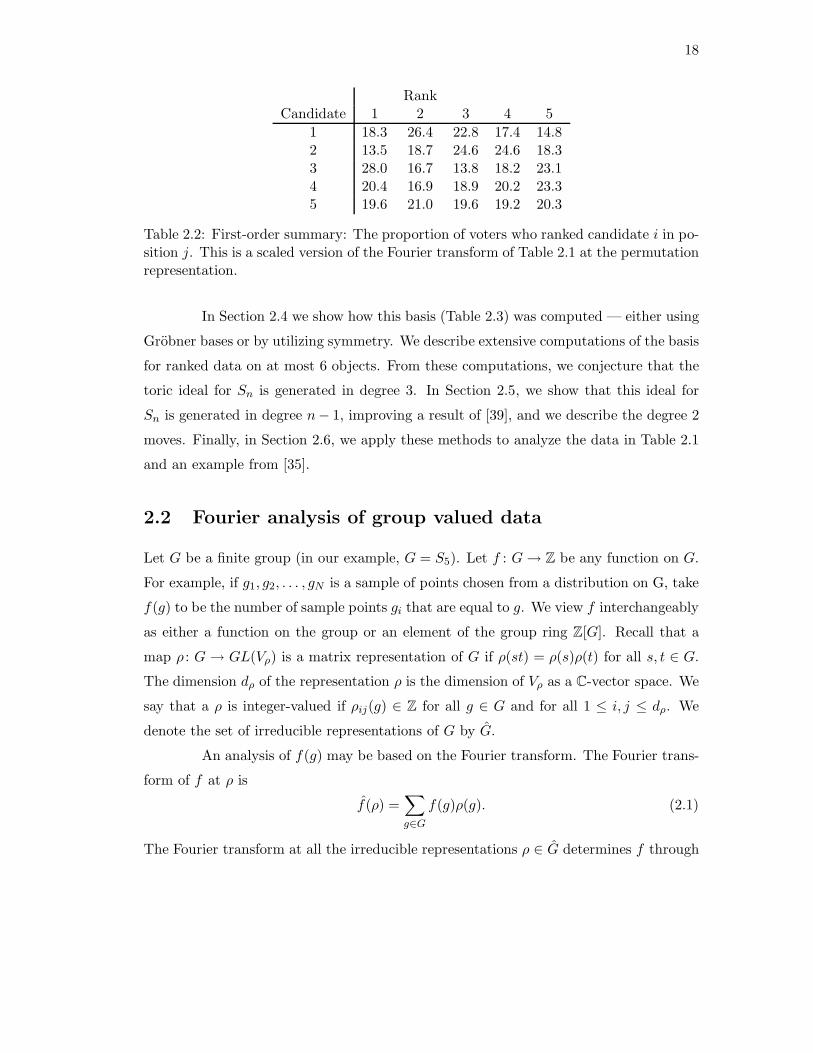
shows a simple summary of the data: the proportion of voters ranking candidate i in
position j. For example, 28.0% of the voters ranked candidate 3 first and 23.1% of the
voters ranked candidate 3 last.
Table 2.2 is a natural summary of the 120 numbers in Table 2.1, but is it an
adequate summary? Does it capture all of the signal in the data? In this paper, we
develop tools to answer such questions using Fourier analysis and algebraic techniques.
In Section 2.2, we give a general exposition of how noncommutative Fourier
analysis can be used to analyze group valued data with summary given by a represen-
tation ρ. In order to use Markov chain Monte Carlo techniques to calibrate the Fourier
analysis, we define an exponential family and toric ideal (as introduced in Section 1.2)
associated to a finite group G and integer representation ρ. A generating set of the toric
ideal can be used to run a Markov chain to sample from data on the group. For example,
the 14 moves in Table 2.3 allow us to randomly sample from the space of data on S5
with fixed first order summary (Table 2.2).
For example, the first entry in Table 2.2 corresponds to the move that adds
one to both of the 53412 and 54321 entries of the data and subtracts one from both the
53421 and 54312 entries. Notice that this move does not change the first order summary.
17
Ranking # votes Ranking # votes Ranking # votes Ranking # votes
54321 29 43521 91 32541 41 21543 3654312 67 43512 84 32514 64 21534 4254231 37 43251 30 32451 34 21453 2454213 24 43215 35 32415 75 21435 2654132 43 43152 38 32154 82 21354 3054123 28 43125 35 32145 74 21345 4053421 57 42531 58 31542 30 15432 4053412 49 42513 66 31524 34 15423 3553241 22 42351 24 31452 40 15342 3653214 22 42315 51 31425 42 15324 1753142 34 42153 52 31254 30 15243 7053124 26 42135 40 31245 34 15234 5052431 54 41532 50 25431 35 14532 5252413 44 41523 45 25413 34 14523 4852341 26 41352 31 25341 40 14352 5152314 24 41325 23 25314 21 14325 2452143 35 41253 22 25143 106 14253 7052134 50 41235 16 25134 79 14235 4551432 50 35421 71 24531 63 13542 3551423 46 35412 61 24513 53 13524 2851342 25 35241 41 24351 44 13452 3751324 19 35214 27 24315 28 13425 3551243 11 35142 45 24153 162 13254 9551234 29 35124 36 24135 96 13245 10245321 31 34521 107 23541 45 12543 3445312 54 34512 133 23514 52 12534 3545231 34 34251 62 23451 53 12453 2945213 24 34215 28 23415 52 12435 2745132 38 34152 87 23154 186 12354 2845123 30 34125 35 23145 172 12345 30
Table 2.1: American Psychological Association (APA) voting data: the number of votersthat ranked the 5 candidates in a given order.
18
RankCandidate 1 2 3 4 5
1 18.3 26.4 22.8 17.4 14.82 13.5 18.7 24.6 24.6 18.33 28.0 16.7 13.8 18.2 23.14 20.4 16.9 18.9 20.2 23.35 19.6 21.0 19.6 19.2 20.3
Table 2.2: First-order summary: The proportion of voters who ranked candidate i in po-sition j. This is a scaled version of the Fourier transform of Table 2.1 at the permutationrepresentation.
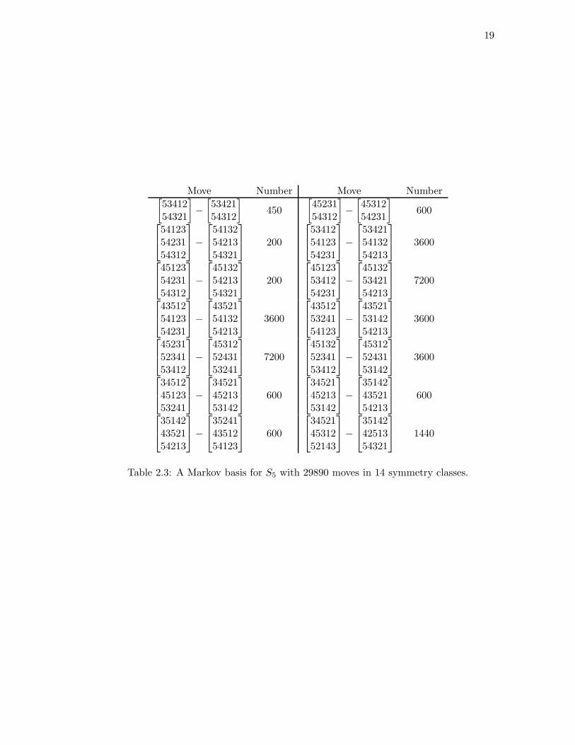
In Section 2.4 we show how this basis (Table 2.3) was computed — either using
Grobner bases or by utilizing symmetry. We describe extensive computations of the basis
for ranked data on at most 6 objects. From these computations, we conjecture that the
toric ideal for Sn is generated in degree 3. In Section 2.5, we show that this ideal for
Sn is generated in degree n− 1, improving a result of [39], and we describe the degree 2
moves. Finally, in Section 2.6, we apply these methods to analyze the data in Table 2.1
and an example from [35].
2.2 Fourier analysis of group valued data
Let G be a finite group (in our example, G = S5). Let f : G → Z be any function on G.
For example, if g1, g2, . . . , gN is a sample of points chosen from a distribution on G, take
f(g) to be the number of sample points gi that are equal to g. We view f interchangeably
as either a function on the group or an element of the group ring Z[G]. Recall that a
map ρ : G → GL(Vρ) is a matrix representation of G if ρ(st) = ρ(s)ρ(t) for all s, t ∈ G.
The dimension dρ of the representation ρ is the dimension of Vρ as a C-vector space. We
say that a ρ is integer-valued if ρij(g) ∈ Z for all g ∈ G and for all 1 ≤ i, j ≤ dρ. We
denote the set of irreducible representations of G by G.
An analysis of f(g) may be based on the Fourier transform. The Fourier trans-
form of f at ρ is
f(ρ) =∑
g∈G
f(g)ρ(g). (2.1)
The Fourier transform at all the irreducible representations ρ ∈ G determines f through
19
Move Number Move Number[
5341254321
]
−
[
5342154312
]
450
[
4523154312
]
−
[
4531254231
]
600
541235423154312
−
541325421354321
200
534125412354231
−
534215413254213
3600
451235423154312
−
451325421354321
200
451235341254231
−
451325342154213
7200
435125412354231
−
435215413254213
3600
435125324154123
−
435215314254213
3600
452315234153412
−
453125243153241
7200
451325234153412
−
453125243153142
3600
345124512353241
−
345214521353142
600
345214521353142
−
351424352154213
600
351424352154213
−
352414351254123
600
345214531252143
−
351424251354321
1440
Table 2.3: A Markov basis for S5 with 29890 moves in 14 symmetry classes.
20
S5 S4,1 S3,2 S3,1,1 S2,2,1 S2,1,1,1 S1,1,1,1,1
d2ρ 1 16 25 36 25 16 1
Data 2286 298 459 78 27 7 0
Table 2.4: Squared length (divided by 120) of the projection of the APA data (Table 2.1)into the 7 isotypic subspaces of S5.
the Fourier inversion formula
f(g) =1
|G|
∑
ρ∈G
dρ Tr(f(ρ)ρ(g−1)), (2.2)
which can be rewritten as f(g) =∑
ρ∈G f |Vρ(g), where
f |Vρ(g) =dρ
|G|
∑
h∈G
χρ(h)f(gh). (2.3)
This decomposition shows the contributions to f from each of the irreducible representa-
tions of G. For example, if a few of the f |Vρ are large, we can analyze these components
in order to understand the structure of f . See [34, 35] for background, proofs, and
previous literature.
Example 2.1. This analysis is most familiar for the cyclic group Cn where it becomes
the discrete Fourier transform
f(j) =n−1∑
k=0
f(k)e−2πijk/n, f(k) =1
n
n−1∑
j=0
f(j)e2πikj/n (2.4)
In (2.4), if a few of the f(j) are much larger than the rest, then f is well understood as
approximately a sum of a few periodic components.
For the symmetric group Sn, the permutation representation assigns permuta-
tion matrices ρ(π) to permutations π. Thus, if f(π) is the number of rankers choosing
π, f(ρ) is a n× n matrix with (i, j) entry the number of rankers ranking item i in posi-
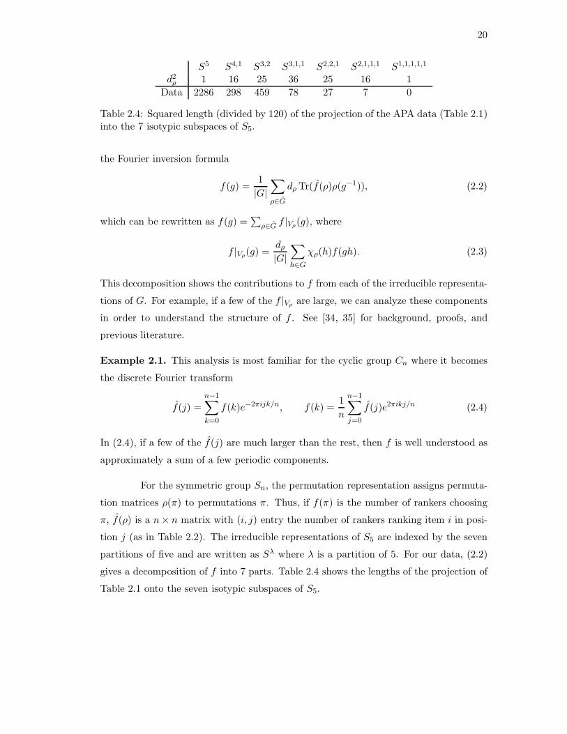
tion j (as in Table 2.2). The irreducible representations of S5 are indexed by the seven
partitions of five and are written as Sλ where λ is a partition of 5. For our data, (2.2)
gives a decomposition of f into 7 parts. Table 2.4 shows the lengths of the projection of
Table 2.1 onto the seven isotypic subspaces of S5.
21
RanksCandidates 1,2 1,3 1,4 1,5 2,3 2,4 2,5 3,4 3,5 4,5
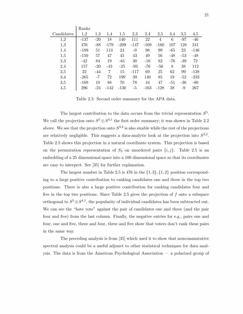
1,2 -137 -20 18 140 111 22 4 6 -97 -461,3 476 -88 -179 -209 -147 -169 -160 107 128 2411,4 -189 51 113 24 -9 98 99 -65 23 -1461,5 -150 57 47 45 43 49 56 -48 -53 -482,3 -42 84 19 -61 30 -16 82 -76 -39 722,4 157 -20 -43 -25 -93 -76 -56 8 38 1122,5 22 -44 7 15 -117 69 25 62 99 -1383,4 -265 -7 72 199 39 140 85 19 -52 -2333,5 -169 10 88 70 78 44 47 -51 -36 -804,5 296 -24 -142 -130 -5 -163 -128 38 -9 267
Table 2.5: Second order summary for the APA data.
The largest contribution to the data occurs from the trivial representation S5.
We call the projection onto S5 ⊕S4,1 the first order summary; it was shown in Table 2.2
above. We see that the projection onto S3,2 is also sizable while the rest of the projections
are relatively negligible. This suggests a data-analytic look at the projection into S3,2.
Table 2.5 shows this projection in a natural coordinate system. This projection is based
on the permutation representation of S5 on unordered pairs {i, j}. Table 2.5 is an
embedding of a 25 dimensional space into a 100 dimensional space so that its coordinates
are easy to interpret. See [35] for further explanation.
The largest number in Table 2.5 is 476 in the {1, 3}, {1, 2} position correspond-
ing to a large positive contribution to ranking candidates one and three in the top two
positions. There is also a large positive contribution for ranking candidates four and
five in the top two positions. Since Table 2.5 gives the projection of f onto a subspace
orthogonal to S5⊕S4,1, the popularity of individual candidates has been subtracted out.
We can see the “hate vote” against the pair of candidates one and three (and the pair
four and five) from the last column. Finally, the negative entries for e.g., pairs one and
four, one and five, three and four, three and five show that voters don’t rank these pairs
in the same way.
The preceding analysis is from [35] which used it to show that noncommutative
spectral analysis could be a useful adjunct to other statistical techniques for data anal-
ysis. The data is from the American Psychological Association — a polarized group of
22
academicians and clinicians who are on very uneasy terms (the organization almost split
in two just after this election). Candidates one and three are in one camp, candidates
four and five from the other. Candidate two seems to be disliked by both camps. The
winner of the election depends on the method of allocating votes. For example, the
Hare system or plurality voting would elect candidate three. However, other widely used
voting methods (Borda’s sum of ranks or Coomb’s elimination system) elect candidate
one. For details and further analysis of the data, see [93].
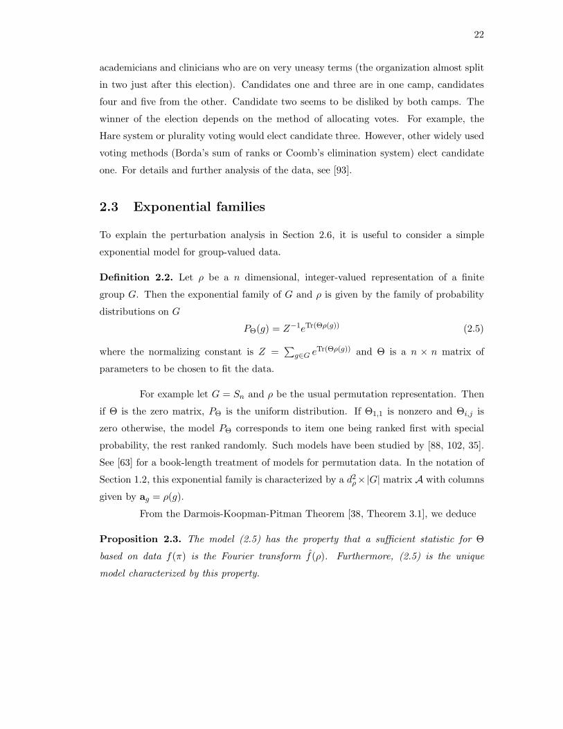
2.3 Exponential families
To explain the perturbation analysis in Section 2.6, it is useful to consider a simple
exponential model for group-valued data.
Definition 2.2. Let ρ be a n dimensional, integer-valued representation of a finite
group G. Then the exponential family of G and ρ is given by the family of probability
distributions on G
PΘ(g) = Z−1eTr(Θρ(g)) (2.5)
where the normalizing constant is Z =∑
g∈G eTr(Θρ(g)) and Θ is a n × n matrix of
parameters to be chosen to fit the data.
For example let G = Sn and ρ be the usual permutation representation. Then
if Θ is the zero matrix, PΘ is the uniform distribution. If Θ1,1 is nonzero and Θi,j is
zero otherwise, the model PΘ corresponds to item one being ranked first with special
probability, the rest ranked randomly. Such models have been studied by [88, 102, 35].
See [63] for a book-length treatment of models for permutation data. In the notation of
Section 1.2, this exponential family is characterized by a d2ρ×|G| matrix A with columns
given by ag = ρ(g).
From the Darmois-Koopman-Pitman Theorem [38, Theorem 3.1], we deduce
Proposition 2.3. The model (2.5) has the property that a sufficient statistic for Θ
based on data f(π) is the Fourier transform f(ρ). Furthermore, (2.5) is the unique
model characterized by this property.
23
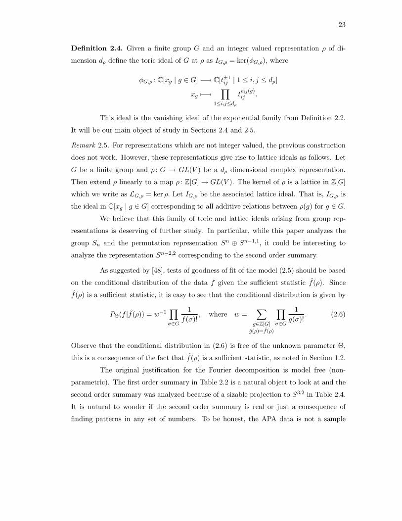
Definition 2.4. Given a finite group G and an integer valued representation ρ of di-
mension dρ define the toric ideal of G at ρ as IG,ρ = ker(φG,ρ), where
φG,ρ : C[xg | g ∈ G] −→ C[t±1ij | 1 ≤ i, j ≤ dρ]
xg 7−→∏
1≤i,j≤dρ
tρij(g)ij .
This ideal is the vanishing ideal of the exponential family from Definition 2.2.
It will be our main object of study in Sections 2.4 and 2.5.
Remark 2.5. For representations which are not integer valued, the previous construction
does not work. However, these representations give rise to lattice ideals as follows. Let
G be a finite group and ρ : G → GL(V ) be a dρ dimensional complex representation.
Then extend ρ linearly to a map ρ : Z[G] → GL(V ). The kernel of ρ is a lattice in Z[G]
which we write as LG,ρ = ker ρ. Let IG,ρ be the associated lattice ideal. That is, IG,ρ is
the ideal in C[xg | g ∈ G] corresponding to all additive relations between ρ(g) for g ∈ G.
We believe that this family of toric and lattice ideals arising from group rep-
resentations is deserving of further study. In particular, while this paper analyzes the
group Sn and the permutation representation Sn ⊕ Sn−1,1, it could be interesting to
analyze the representation Sn−2,2 corresponding to the second order summary.
As suggested by [48], tests of goodness of fit of the model (2.5) should be based
on the conditional distribution of the data f given the sufficient statistic f(ρ). Since
f(ρ) is a sufficient statistic, it is easy to see that the conditional distribution is given by
PΘ(f |f(ρ)) = w−1∏
σ∈G
1
f(σ)!, where w =
∑
g∈Z[G]
g(ρ)=f(ρ)
∏
σ∈G
1
g(σ)!. (2.6)
Observe that the conditional distribution in (2.6) is free of the unknown parameter Θ,
this is a consequence of the fact that f(ρ) is a sufficient statistic, as noted in Section 1.2.
The original justification for the Fourier decomposition is model free (non-
parametric). The first order summary in Table 2.2 is a natural object to look at and the
second order summary was analyzed because of a sizable projection to S3,2 in Table 2.4.
It is natural to wonder if the second order summary is real or just a consequence of
finding patterns in any set of numbers. To be honest, the APA data is not a sample
24
(those 5,972 who choose to vote are likely to be quite different from the bulk of the
100,000 or so APA members). If the first order summary is accepted “as is”, the largest
probability model for which f(ρ) captures all the structure in the data is the exponential
family (2.5). It seems natural to use the conditional distribution of the data given f(ρ)
as a way of perturbing things. The uniform distribution on data with fixed f(ρ) is a
much more aggressive perturbation procedure. Both are computed and compared in
Section 2.6.
2.4 Computing Markov bases for permutation data
To carry out a test based on Fisher’s principles, we use Markov chain Monte Carlo to
draw samples from the distribution (2.6).
Definition 2.6. A Markov basis for a finite group G and a representation ρ is a finite
subset of “moves” g1, . . . , gB ∈ Z[G] with gi(ρ) = 0 such that any two elements in N[G]
with the same Fourier transform at the representation ρ can be connected by a sequence
of moves in that subset.
In [39] it was explained how Grobner basis techniques could be applied to find
such Markov bases.
Proposition 2.7. A generating set of IG,ρ (see Definition 2.4) is a Markov basis for the
group G and the representation ρ.
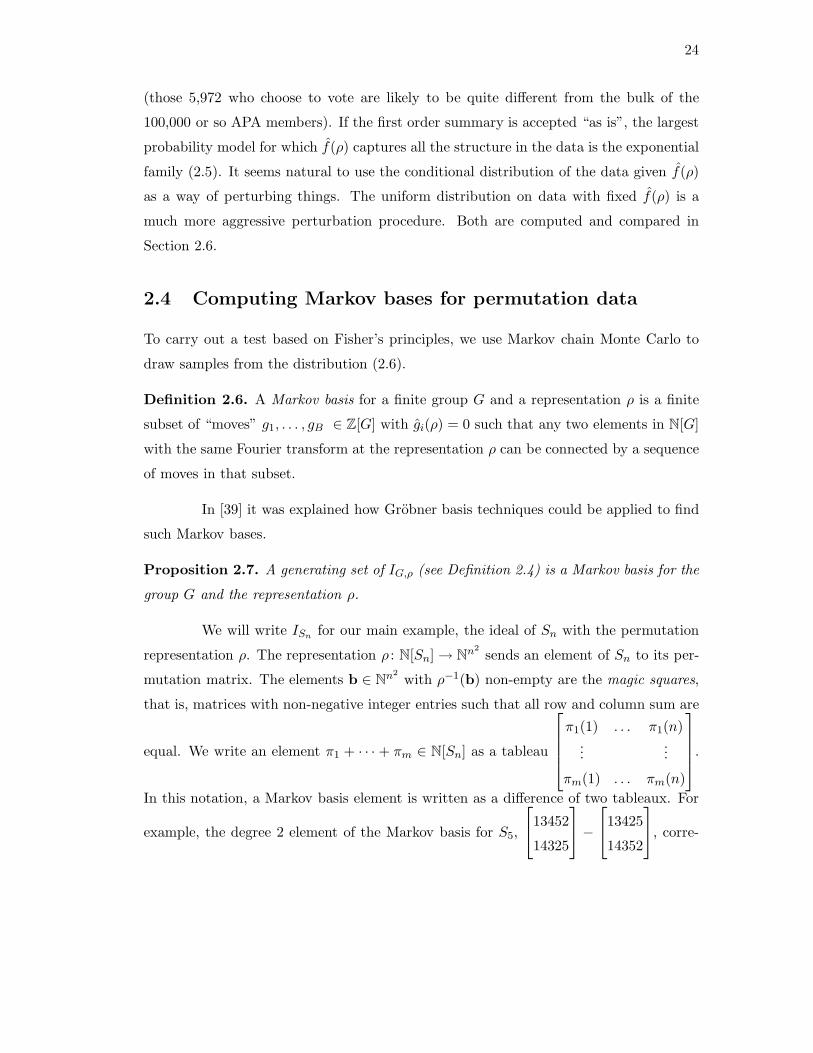
We will write ISn for our main example, the ideal of Sn with the permutation
representation ρ. The representation ρ : N[Sn] → Nn2
sends an element of Sn to its per-
mutation matrix. The elements b ∈ Nn2
with ρ−1(b) non-empty are the magic squares,
that is, matrices with non-negative integer entries such that all row and column sum are
equal. We write an element π1 + · · · + πm ∈ N[Sn] as a tableau
π1(1) . . . π1(n)...
...
πm(1) . . . πm(n)
.
In this notation, a Markov basis element is written as a difference of two tableaux. For
example, the degree 2 element of the Markov basis for S5,
13452
14325
−
13425
14352
, corre-

25
S3 Move Number S4 Move Number
123231312
−
132213321
1
[
12342143
]
−
[
12432134
]
18
231424314123
−
213424134321
144
132421343214
−
123423143124
16
Table 2.6: Markov bases for S3 and S4 and the size of their symmetry classes.
sponds to adding one to the entries 13452 and 14325 in Table 2.1 and subtracting one
from the entries 13425 and 14352.
At the time of writing [39], finding a Grobner basis for IS5 was computationally
infeasible. Due to an increase in computing power and the development of the software
4ti2 [53], we were able to compute a Grobner and a minimal basis of IS5 .
This computation involved finding a Grobner basis of a toric ideal involving 120
indeterminates. It took 4ti2 approximately 90 hours of CPU time on a 2GHz machine
and produced a basis with 45,825 elements. The Markov basis had 29890 elements,
1050 of degree 2 and 28840 of degree 3, see Tables 2.3 and 2.7. Using 4ti2, we have
also computed Markov bases of the ideals ISn for n = 3 and n = 4, they are shown in
Table 2.6.
Although the calculation for S6 is currently not possible using Grobner basis
methods, there is a natural group action that reduces the complexity of this problem.
The group Sn × Sn acts on Nn2
by permuting rows and columns. If we permute the
rows and columns of a magic square, we still have a magic square, therefore, this action
lifts to a group action on the Markov basis of ISn . In terms of tableaux, one copy of Sn
acts by permuting columns of the tableau, the other acts by permuting the labels in the
tableau. We have calculated orbits under this action; notice that the symmetrized bases
are remarkably small (Table 2.7).
To calculate a Markov basis for IS6, we had to construct the fiber over every
magic square with sum at most 5 (by Theorem 2.10) and then pick moves such that

26
every fiber is connected by these moves [98, Theorem 5.3]. For degrees 2 and 3 this was
relatively straightforward (e.g., there are 20,933,840 six by six magic squares with sum
3). For these degrees, we constructed all squares and then calculated orbits of the group
action and calculated the fiber for each orbit (there were 11 orbits in degree 2 and 103
in degree 3).
However, there are 1,047,649,905 six by six magic squares of degree 4 and
30,767,936,616 of degree 5 [7], so complete enumeration was not possible. Instead, we
first randomly generated millions of magic squares with sums 4 or 5 using another Markov
chain. We broke these down into orbits, keeping track of the number of squares we had
found. For example, we needed to generate 30 million squares of degree 5 to find a
representative for each orbit. We were left with 2804 orbits for degree 4 and 65481 orbits
for degree 5. For degree 5, the proof of Theorem 2.10 shows that we only need to consider
magic squares with norm squared less that 50, leaving 13196 orbits to check. The fibers
were calculated by a depth first search with pruning. Remarkably, the computation
showed that IS6 is generated in degree three.
Theorem 2.8. The ideal ISn is minimally generated by 57,150 binomials of degree two
and 7,056,420 binomials of degree three. The degree two generators form seven orbits
under the action of S6×S6; the degree three generators form 51 orbits under this action.
The entire calculation for S6 took about 2 weeks, with the vast majority of
the time spent calculating orbits of degree 5 squares. Our data and code (in perl) are
available for download at http://math.berkeley.edu/∼eriksson. The code could be
easily adapted to calculate other Markov bases with a good degree bound and a large
symmetry group. Our calculations (see Table 2.7) suggest the following conjecture:
Conjecture 2.9. The ideal ISn is generated in degree 3.
2.5 Structure of the toric ideal ISn
Theorem 6.1 of [39] shows that every reverse lexicographic Grobner basis of ISn has
degree at most n. By considering only minimal generators and not a full Grobner basis,
we are able to strengthen this degree bound.
27
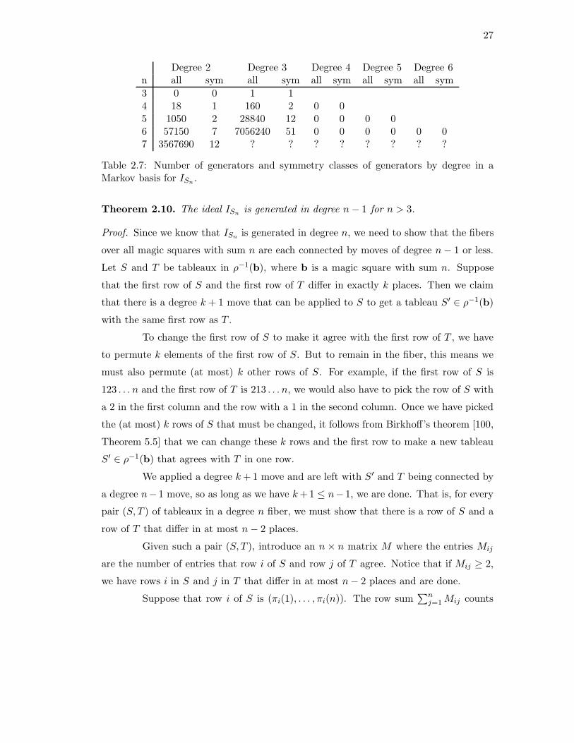
Degree 2 Degree 3 Degree 4 Degree 5 Degree 6n all sym all sym all sym all sym all sym
3 0 0 1 14 18 1 160 2 0 05 1050 2 28840 12 0 0 0 06 57150 7 7056240 51 0 0 0 0 0 07 3567690 12 ? ? ? ? ? ? ? ?
Table 2.7: Number of generators and symmetry classes of generators by degree in aMarkov basis for ISn .
Theorem 2.10. The ideal ISn is generated in degree n − 1 for n > 3.
Proof. Since we know that ISn is generated in degree n, we need to show that the fibers
over all magic squares with sum n are each connected by moves of degree n − 1 or less.
Let S and T be tableaux in ρ−1(b), where b is a magic square with sum n. Suppose
that the first row of S and the first row of T differ in exactly k places. Then we claim
that there is a degree k + 1 move that can be applied to S to get a tableau S′ ∈ ρ−1(b)
with the same first row as T .
To change the first row of S to make it agree with the first row of T , we have
to permute k elements of the first row of S. But to remain in the fiber, this means we
must also permute (at most) k other rows of S. For example, if the first row of S is
123 . . . n and the first row of T is 213 . . . n, we would also have to pick the row of S with
a 2 in the first column and the row with a 1 in the second column. Once we have picked
the (at most) k rows of S that must be changed, it follows from Birkhoff’s theorem [100,
Theorem 5.5] that we can change these k rows and the first row to make a new tableau
S′ ∈ ρ−1(b) that agrees with T in one row.
We applied a degree k + 1 move and are left with S′ and T being connected by
a degree n− 1 move, so as long as we have k +1 ≤ n− 1, we are done. That is, for every
pair (S, T ) of tableaux in a degree n fiber, we must show that there is a row of S and a
row of T that differ in at most n − 2 places.
Given such a pair (S, T ), introduce an n × n matrix M where the entries Mij
are the number of entries that row i of S and row j of T agree. Notice that if Mij ≥ 2,
we have rows i in S and j in T that differ in at most n − 2 places and are done.
Suppose that row i of S is (πi(1), . . . , πi(n)). The row sum∑n
j=1 Mij counts
28
the total number of times that πi(j) appears in column j for each j. This is exactly∑n
k=1 b(k, π(k)). Summing over all rows, we see that every entry of b gets counted its
cardinality number of times. That is,
∑
1≤i,j≤n
Mij =∑
1≤i,j≤n
b(i, j)2 = ||b||2
Now since each row of b sums to n, we have that ||b||2 ≥ n2, with equality only if
b(i, j) = 1 for all i, j. Notice that if ||b||2 > n2, then one of the Mij must be larger than
1, and we are done.
Therefore, we only have to consider the fiber over b1 =
( 1 1 ... 1...
...1 1 ... 1
)
. Elements
of this fiber are tableaux such that every row and every column is a permutation of
{1, . . . , n} (“Latin squares”). Two tableaux are connected by a degree n−1 move if they
have a row in common. We claim that if n > 3, this graph is connected. (Note that for
n = 3, there are two components and a degree 3 move for S3, see Table 2.7.)
For fixed ν ∈ Sn, the set Tν of all tableaux in ρ−1(b1) that have ν as a row is
connected by definition. Form the graph Gn where the vertices are elements ν ∈ Sn and
there is an edge between λ and ν if λ and ν occur in a tableau together. Then if this
graph is connected, the whole fiber over b1 is connected by degree n − 1 moves.
First, we claim that λ and ν occur together in a tableau if and only if λ is
a derangement with respect to ν (i.e., if λ and ν are disjoint from each other). The
derangement condition is clearly necessary. Sufficiency follows from Birkhoff’s theorem:
if λ is a derangement with respect to ν, then the square b1−ρ(λ)−ρ(ν) has non-negative
entries and row and column sums n − 2, therefore, it it the sum of n − 2 permutation
matrices. Thus, Gn is the graph where two permutations are connected by an edge when
they are disjoint.
Now note that [1, 2, . . . , n − 2, n − 1, n] and [3, 4, . . . , n, 1, 2] are connected in
Gn since the second is a cyclic shift of the first. Then, if n > 3, [3, 4, . . . , n, 1, 2] and
[1, 2, . . . , n−2, n, n−1] are also connected. Thus [1, 2, . . . , n] and [1, 2, . . . , n−2, n, n−1]
are connected, so applying transpositions keeps us in the same connected component of
Gn. But Sn is generated by transpositions, so Gn is connected and therefore ρ−1(b1) is
connected by moves of degree n − 1.

29
Theorem 2.10 gives rise to the question of whether there exists a Grobner basis
of degree n − 1 for ISn .
Definition 2.11. Let I be an ideal in m unknowns, and let C[ω] be the equivalence
class of vectors in Rm that give the same Grobner basis as ω, i.e.,
C[ω] ={
ω′ ∈ Rm | inω′(g) = inω(g) for all g ∈ G
}
,
where G is the reduced Grobner basis of I with respect to ω. Then the Grobner fan of
I, denoted GF (I) is the set of closed cones C[ω] for all ω ∈ Rm.
Remark 2.12. We attempted to find the entire Grobner fan for n = 4 using the software
packages CaTS [57] and gfan [56]. This computation failed for both programs after
several weeks due to excessive memory usage of over 3 GB. However, before failing, we
were able to calculate 805,671 Grobner bases with CaTS and 2,973,312 Grobner bases
with gfan. Every one of these Grobner bases contained elements of degree 4, in contrast
with the Markov basis of degree 3. Furthermore, our Grobner basis for S5 contained
degree 5 elements. Therefore, it is possible that the degree n Grobner basis of [39] is the
Grobner basis of smallest degree.
While ISn is difficult to compute, it is easy to classify the degree 2 part of the
Markov basis.
Proposition 2.13. Let D2(n) be the number of degree 2 moves, up to symmetry, in a
Markov basis for Sn. Then
D2(n) = D2(n − 1) +
⌊n2⌋
∑
k=2
(2k−1 − 1)[qn−2k]
k∏
i=1
1
1 − qi,
where [qj](∑
aiqi) := aj . For example, D2(9) = 47.
Proof. First assume that all entries of the magic square b are either 1 or 0. Then the
squares with non-trivial ρ−1(b) are those that can be put in a block diagonal form with
k ≥ 2 blocks and each block of size at least 2. Such a magic square has a fiber of size
2k−1, corresponding to choosing, for each block, an orientation of the two permutations
that sum to that block (since the order of the rows in a tableau don’t matter, there
30
S5 S4,1 S3,2 S3,1,1 S2,2,1 S2,1,1,1 S1,1,1,1,1
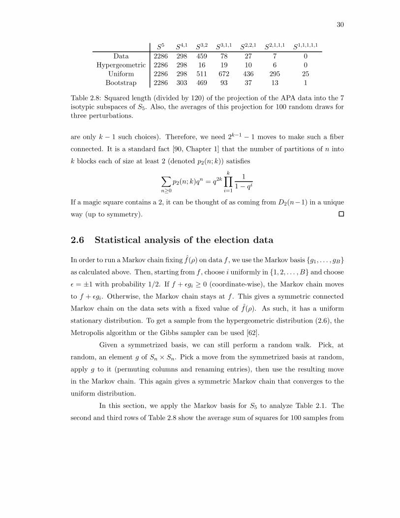
Data 2286 298 459 78 27 7 0Hypergeometric 2286 298 16 19 10 6 0
Uniform 2286 298 511 672 436 295 25Bootstrap 2286 303 469 93 37 13 1
Table 2.8: Squared length (divided by 120) of the projection of the APA data into the 7isotypic subspaces of S5. Also, the averages of this projection for 100 random draws forthree perturbations.
are only k − 1 such choices). Therefore, we need 2k−1 − 1 moves to make such a fiber
connected. It is a standard fact [90, Chapter 1] that the number of partitions of n into
k blocks each of size at least 2 (denoted p2(n; k)) satisfies
∑
n≥0
p2(n; k)qn = q2kk∏
i=1
1
1 − qi
If a magic square contains a 2, it can be thought of as coming from D2(n−1) in a unique
way (up to symmetry).
2.6 Statistical analysis of the election data
In order to run a Markov chain fixing f(ρ) on data f , we use the Markov basis {g1, . . . , gB}
as calculated above. Then, starting from f , choose i uniformly in {1, 2, . . . , B} and choose
ǫ = ±1 with probability 1/2. If f + ǫgi ≥ 0 (coordinate-wise), the Markov chain moves
to f + ǫgi. Otherwise, the Markov chain stays at f . This gives a symmetric connected
Markov chain on the data sets with a fixed value of f(ρ). As such, it has a uniform
stationary distribution. To get a sample from the hypergeometric distribution (2.6), the
Metropolis algorithm or the Gibbs sampler can be used [62].
Given a symmetrized basis, we can still perform a random walk. Pick, at
random, an element g of Sn × Sn. Pick a move from the symmetrized basis at random,
apply g to it (permuting columns and renaming entries), then use the resulting move
in the Markov chain. This again gives a symmetric Markov chain that converges to the
uniform distribution.
In this section, we apply the Markov basis for S5 to analyze Table 2.1. The
second and third rows of Table 2.8 show the average sum of squares for 100 samples from
31
Metropolis
Length of projection
Fre
quen
cy
10 15 20 25
05
1015
20
Uniform
Length of projection
Fre
quen
cy
200 300 400 500 600 700 800
05
1015
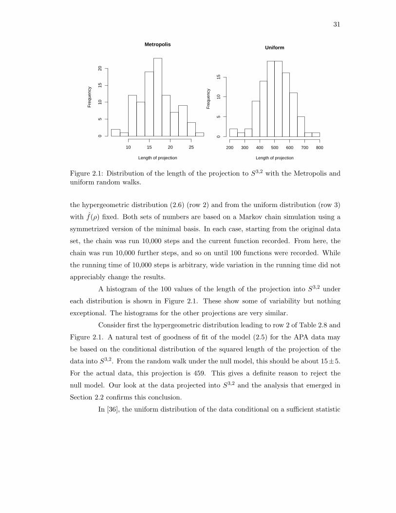
Figure 2.1: Distribution of the length of the projection to S3,2 with the Metropolis anduniform random walks.
the hypergeometric distribution (2.6) (row 2) and from the uniform distribution (row 3)
with f(ρ) fixed. Both sets of numbers are based on a Markov chain simulation using a
symmetrized version of the minimal basis. In each case, starting from the original data
set, the chain was run 10,000 steps and the current function recorded. From here, the
chain was run 10,000 further steps, and so on until 100 functions were recorded. While
the running time of 10,000 steps is arbitrary, wide variation in the running time did not
appreciably change the results.
A histogram of the 100 values of the length of the projection into S3,2 under
each distribution is shown in Figure 2.1. These show some of variability but nothing
exceptional. The histograms for the other projections are very similar.
Consider first the hypergeometric distribution leading to row 2 of Table 2.8 and
Figure 2.1. A natural test of goodness of fit of the model (2.5) for the APA data may
be based on the conditional distribution of the squared length of the projection of the
data into S3,2. From the random walk under the null model, this should be about 15±5.
For the actual data, this projection is 459. This gives a definite reason to reject the
null model. Our look at the data projected into S3,2 and the analysis that emerged in
Section 2.2 confirms this conclusion.
In [36], the uniform distribution of the data conditional on a sufficient statistic
32
was suggested as an antagonistic alternative to the null hypothesis when the data strongly
rejects a null model. The idea is to help quantify if the data is really far from the null,
or practically close to the null and just rejected because of a small deviation but a large
sample size [36]. From Figure 2.1, we see that the actual projected length 459 is roughly
typical of a pick from the uniform. This affirms the strong rejection of (2.5) and points
to a need to look at the structure of the higher order projection on its own terms.
An appropriate stability analysis was left open in [35]. If the data in Table 2.1
were a sample from a larger population, the sampling variability adds noise to the signal.
How stable is the analysis above to natural stochastic perturbations? One standard
approach is shown in the last row of Table 2.8. This is based on a boot-strap perturbation
of the data in Table 2.1. Here, the votes of all 5972 rankers are put in a hat and a sample
of size 5972 is drawn from the hat with replacement to give a new data set. The sum of
squares decomposition is repeated. This resampling step (from the original population)
was repeated 100 times. The entries in the last row of Table 2.8 show the average squared
length of these projections. We see that they do not vary much from the original sum of
squares. While not reported here, the boot-strap analogue of the second order analysis
in Table 2.8 was quite stable. We conclude that sampling variability is not an important
issue for this example.
2.7 Statistical analysis of an S4 example
In [39] an S4 example was analyzed. However, the data was analyzed using only the uni-
form distribution, which only tells half of the story. The analysis under hypergeometric
sampling gives an important supplement. Briefly, a sample of 2262 German citizens were
asked to rank order the desirability of four political goals:
1. Maintain order;
2. Give people more say in government;
3. Fight rising prices;
4. Protect freedom of speech.

33
1234 137 2134 48 3124 330 4123 211243 29 2143 23 3142 294 4132 301324 309 2314 61 3214 117 4213 291342 255 2341 55 3241 69 4231 521423 52 2413 33 3412 70 4312 351432 93 2431 59 3421 34 4321 27
Table 2.9: The number of German citizens who ranked the four political goals in a givenorder.
RankGoal 1 2 3 4
1 875 279 914 1942 746 433 742 3413 345 773 419 7254 296 777 187 1002
Table 2.10: First order summary for the S4 ranked data in Table 2.9.
The data appears in Table 2.9 and the first order summary in Table 2.10. The sizes
of the projections for the data and the random walks appear in Table 2.11. We have
corrected a typographical error in the data in [39], the 2431 entry should be 59.
The projection of the data into the second order subspace S2,2 has squared
length 268. The boot-strap analysis (Line 4 in Table 2.11) shows this is stable under
sampling perturbations. The hypergeometric analysis (line 2 of Table 2.11) suggests that
for the specific data, relatively large projections onto the second order space are typical,
even if the first order model holds. This is quite different than the previous example.
Still, the observed 268 is sufficiently much larger than 169 that a look at the second
order projection is warranted. The uniform analysis points to the actual projection
S4 S3,1 S2,2 S2,1,1 S1,1,1,1
Data 462 381 268 49 4Metropolis 462 381 169 37 8Uniform 462 381 277 228 80
Bootstrap 462 381 269 56 7
Table 2.11: Length of the projections onto the five isotypic subspaces for the S4 dataand three perturbations.

34
being typical, this again suggests a serious look at the second order projection.
Remark 2.14. We note that the software package LattE [28] can be used to count how
many data sets have a given first order summary. For our S4 example (Table 2.9), these
correspond to lattice points inside a convex polytope with 6285 vertices in R24. LattE
quickly computes that there are 11606690287805167142987310121 (approximately 1028)
elements of N[S4] with the same first order summary as our S4 example. However, LattE
was unable to compute this number for the S5 data (Table 2.1).
35
Chapter 3
Toric ideals of homogeneous
phylogenetic models
In this chapter, we consider the fully observed homogeneous phylogenetic model
That is to say, every node of the tree is an observed, binary random variable and the
transition probabilities are given by the same matrix on each edge of the tree. The ideal
of invariants of this model is a toric ideal, returning to a major theme from Chapter 2.
We are able to compute the Grobner basis and minimal generating set for
this ideal for trees with up to 11 nodes. These are the first non-trivial Grobner bases
calculations in 211 = 2048 indeterminates. We conjecture that there is a quadratic
Grobner basis for binary trees, but that generators of degree n are required for certain
non-binary trees on n nodes. The polytopes associated with these toric ideals display
interesting finiteness properties. We describe the polytope for an infinite family of binary
trees and conjecture (based on extensive computations) that there is a universal bound
on the number of vertices of the polytope of a binary tree. This polytope is meaningful
statistically — it solves the problem of parametric inference. Parametric inference solves
the maximum a posteriori inference problem for all model parameters simultaneously.
See [33] for an example of parametric inference applied to the biological problem of
sequence alignment.
It should be noted that since all nodes are observed, the invariant calculations
will not themselves be useful for phylogenetics. Furthermore, the homogeneous model
36
is not very biologically relevant. However, the fully observed homogeneous model is
particularly attractive due to the small number of parameters and the toric structure.
The material in this chapter comes from [43].
3.1 Homogeneous phylogenetic models
In this chapter we consider the homogeneous Markov model on a tree T where all tran-
sition matrices are equal, all nodes are binary and observable, and the root has uniform
distribution. We write A =
θ00 θ01
θ10 θ11
for the transition matrices. Let ρ(v) denote the
parent of v ∈ T .
The probability of observing i at a node v is computed from the parent of v by
P (Xv = i) = θ0iP (Xρ(v) = 0) + θ1iP (Xρ(v) = 1).
We are interested in the algebraic relations satisfied by the joint distribution
pi1i2...in := P (X1 = i1, . . . ,Xn = in).
Writing the joint distribution in terms of the model parameters θ00, θ01, θ10, θ11, we have
pi1i2...in =
n∏
j=2
θiρ(j)ij (3.1)
where the nodes of the tree are labeled 1 to n starting with the root. That is, the
probability of observing a certain labeling of the tree is the product of the θij that
correspond to the transitions on all edges of the tree. The indeterminates θij parameterize
a toric variety of dimension 4 in R2n
. We let IT be the corresponding toric ideal, called
the ideal of phylogenetic invariants. In the notation of [98], the toric ideal IT is specified
by the 4 by 2n configuration AT , where the column ai consists of the exponent vector of
the θij in (3.1). We order the rows (θ00, θ01, θ10, θ11). Let PT be the convex hull of the
columns of AT .
We are interested in two questions from [72]. First, which relations on the joint
probabilities pi1...in does the model imply? This problem is solved by giving generators
of the ideal of invariants IT .
37
In Section 3.2, we study the generators of this ideal. Our main accomplishment
is the computation of Grobner and Markov bases for all binary trees with 11 nodes. These
are computations in 2048 indeterminates, which we believe to be the largest number of
indeterminates yet in a Grobner basis calculation. We also calculate generating sets for
all trees on at most 9 nodes. Based on this evidence, we conjecture that if T is binary,
then the ideal IT has a quadratic generating set. However, our calculations suggest that
relations of degree n are necessary to generate IT for certain trees with n nodes.
Our second goal is to determine, given a labeling of the tree T , if we can identify
parameters θij such that the labeling is the most likely among all labelings. This problem
is solved by computing the normal fan of the toric variety in the sense of [50].
In Section 3.3, we study this normal fan and the polytope PT . Our main result,
Theorem 3.7, is an explicit description of the polytope PT for an infinite family of binary
trees. For this family, PT always has 8 vertices and 6 facets which we characterize. We
also present extensive calculations of PT for various trees and conjecture that there is a
bound on the number of vertices of PT as T ranges over all binary trees.
Example 3.1. Let T be a path with 3 nodes. Then
AT =
2 1 0 0 1 0 0 0
0 1 1 1 0 1 0 0
0 0 1 0 1 1 1 0
0 0 0 1 0 0 1 2
,
the polytope PT is three dimensional with seven vertices and six facets. The toric ideal
of the path of length 3 is generated by 6 binomials
IT = 〈p101 − p010, p001p100 − p000p010,
p011p100 − p001p110, p011p110 − p010p111,
p2001p111 − p000p
2011, p2
100p111 − p000p2110〉.
3.2 Toric ideals
The toric ideals IT are homogeneous, since all monomials in (3.1) have the same degree
n − 1. Thus they define projective toric varieties YT .
38
Recall that a projective toric variety given by a configuration A = (a1, . . . ,ak)
is covered by the affine toric varieties given by A− ai. An affine toric variety defined by
a configuration B is said to be smooth if the semigroup NB is isomorphic to Nr for some
r [99, Lemma 2.2].
Proposition 3.2. The projective toric variety YT of a binary tree T is not smooth.
Proof. Recall that the columns of the configuration AT are indexed by 0/1-labelings of
the tree T . Look at the affine chart IA−a0...0 , where a0...0 corresponds to the all zero tree.
On this chart, write ai = ai − a0...0. The cone R≥0(A− a0...0) is simplicial, with extreme
rays coming from the following labelings of the tree: let 10 . . . 0 be the tree with a 1 at
the root and zeros everywhere else, 0 . . . 01 be the tree with a 1 at a single leaf and zeros
everywhere else, and 1 . . . 1 be the tree with all ones. That is, three generators of the
semigroup are
a10...0 = (n − 3, 0, 2, 0) − a0...0 = (−2, 0, 2, 0)
a0...01 = (n − 2, 1, 0, 0) − a0...0 = (−1, 1, 0, 0)
a1...1 = (0, 0, 0, n − 1) − a0...0 = (−n + 1, 0, 0, n − 1)
Now it is easy to check that, for example, the point a∗ = (−n+1, 0, 2, n−3) does not lie in
the semigroup generated by the three previous elements. Furthermore, this point comes
from the labeling of a tree (the tree with all labels one except for 2 sibling leaves, their
parent, and a single other leaf who are labeled zero). Thus it lies in the configuration
A−a0...0, so the semigroup requires at least 4 generators. Therefore, N(A−a0...0) is not
isomorphic to N3 and so the toric variety YT is not smooth.
Using 4ti2 [53], Grobner and Markov bases for the ideal IT were computed
for all trees with at most 9 nodes as well as selected trees with 10 and 11 nodes. This
took about 6 weeks of computer time in total on a 2GHz computer. The computations
in 2048 variables (trees with 11 nodes) each took as long as a week and required over 2
GB of memory.
Details about the Markov bases for all binary trees with at most 11 nodes are
shown in Table 3.1. These computations lead us to make the following conjectures.
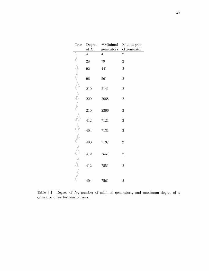
39
Tree Degree #Minimal Max degreeof IT generators of generator
4 4 2
28 79 2
92 441 2
96 561 2
210 2141 2
220 2068 2
210 2266 2
412 7121 2
404 7131 2
400 7137 2
412 7551 2
412 7551 2
404 7561 2
Table 3.1: Degree of IT , number of minimal generators, and maximum degree of agenerator of IT for binary trees.
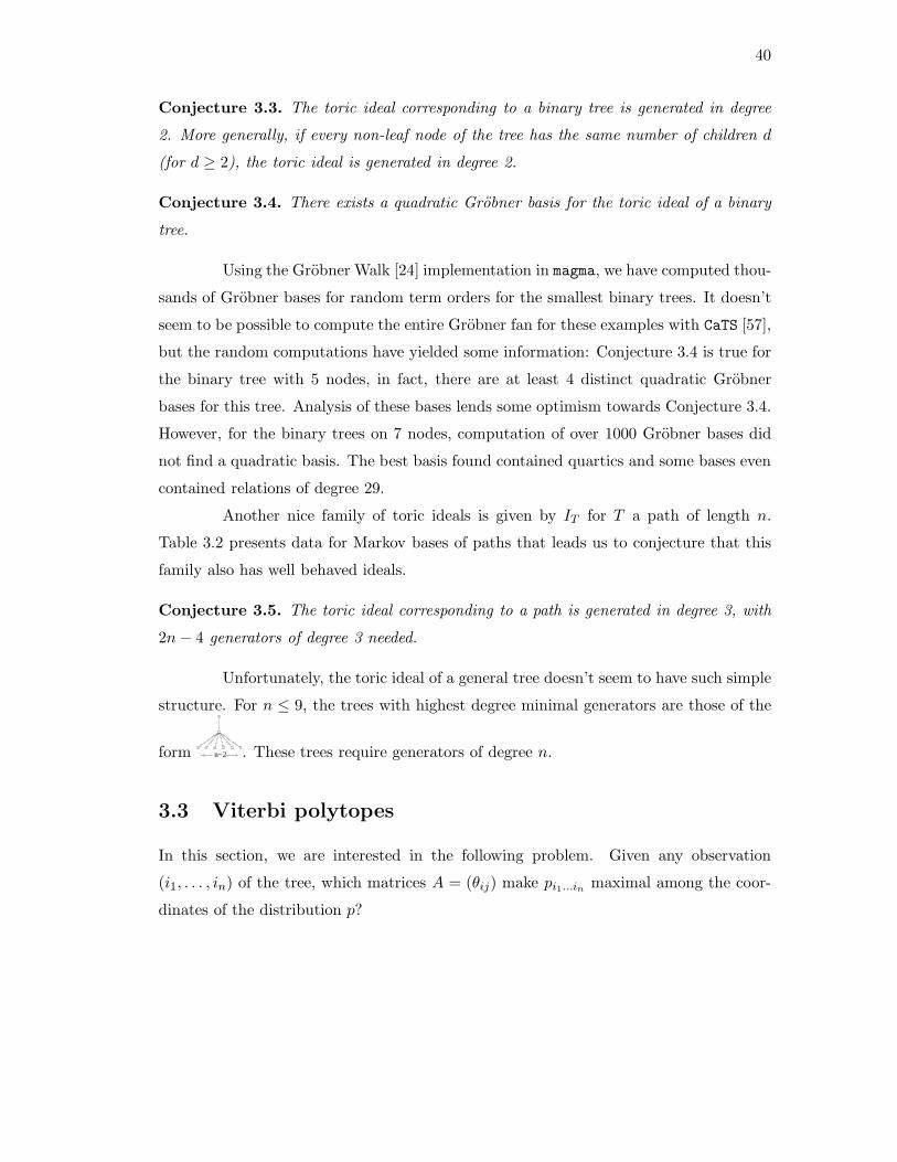
40
Conjecture 3.3. The toric ideal corresponding to a binary tree is generated in degree
2. More generally, if every non-leaf node of the tree has the same number of children d
(for d ≥ 2), the toric ideal is generated in degree 2.
Conjecture 3.4. There exists a quadratic Grobner basis for the toric ideal of a binary
tree.
Using the Grobner Walk [24] implementation in magma, we have computed thou-
sands of Grobner bases for random term orders for the smallest binary trees. It doesn’t
seem to be possible to compute the entire Grobner fan for these examples with CaTS [57],
but the random computations have yielded some information: Conjecture 3.4 is true for
the binary tree with 5 nodes, in fact, there are at least 4 distinct quadratic Grobner
bases for this tree. Analysis of these bases lends some optimism towards Conjecture 3.4.
However, for the binary trees on 7 nodes, computation of over 1000 Grobner bases did
not find a quadratic basis. The best basis found contained quartics and some bases even
contained relations of degree 29.
Another nice family of toric ideals is given by IT for T a path of length n.
Table 3.2 presents data for Markov bases of paths that leads us to conjecture that this
family also has well behaved ideals.
Conjecture 3.5. The toric ideal corresponding to a path is generated in degree 3, with
2n − 4 generators of degree 3 needed.
Unfortunately, the toric ideal of a general tree doesn’t seem to have such simple
structure. For n ≤ 9, the trees with highest degree minimal generators are those of the
form n−2 . These trees require generators of degree n.
3.3 Viterbi polytopes
In this section, we are interested in the following problem. Given any observation
(i1, . . . , in) of the tree, which matrices A = (θij) make pi1...in maximal among the coor-
dinates of the distribution p?
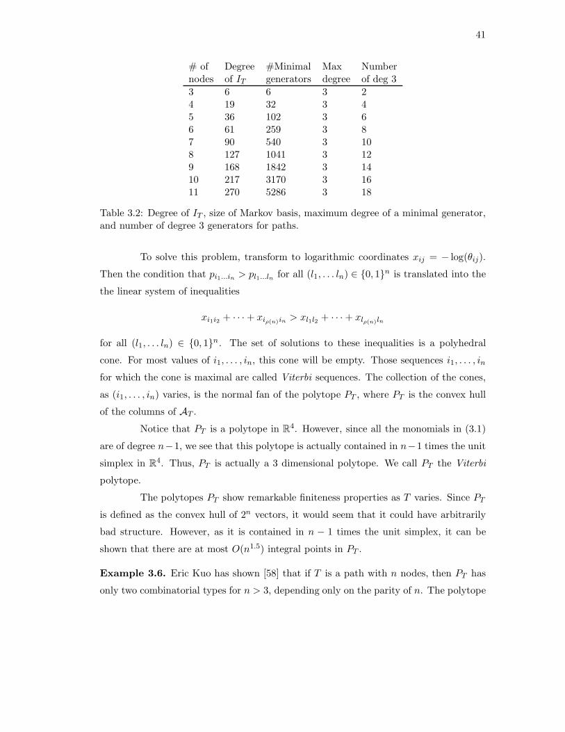
41
# of Degree #Minimal Max Numbernodes of IT generators degree of deg 3
3 6 6 3 24 19 32 3 45 36 102 3 66 61 259 3 87 90 540 3 108 127 1041 3 129 168 1842 3 1410 217 3170 3 1611 270 5286 3 18
Table 3.2: Degree of IT , size of Markov basis, maximum degree of a minimal generator,and number of degree 3 generators for paths.
To solve this problem, transform to logarithmic coordinates xij = − log(θij).
Then the condition that pi1...in > pl1...ln for all (l1, . . . ln) ∈ {0, 1}n is translated into the
the linear system of inequalities
xi1i2 + · · · + xiρ(n)in > xl1l2 + · · · + xlρ(n)ln
for all (l1, . . . ln) ∈ {0, 1}n. The set of solutions to these inequalities is a polyhedral
cone. For most values of i1, . . . , in, this cone will be empty. Those sequences i1, . . . , in
for which the cone is maximal are called Viterbi sequences. The collection of the cones,
as (i1, . . . , in) varies, is the normal fan of the polytope PT , where PT is the convex hull
of the columns of AT .
Notice that PT is a polytope in R4. However, since all the monomials in (3.1)
are of degree n−1, we see that this polytope is actually contained in n−1 times the unit
simplex in R4. Thus, PT is actually a 3 dimensional polytope. We call PT the Viterbi
polytope.
The polytopes PT show remarkable finiteness properties as T varies. Since PT
is defined as the convex hull of 2n vectors, it would seem that it could have arbitrarily
bad structure. However, as it is contained in n − 1 times the unit simplex, it can be
shown that there are at most O(n1.5) integral points in PT .
Example 3.6. Eric Kuo has shown [58] that if T is a path with n nodes, then PT has
only two combinatorial types for n > 3, depending only on the parity of n. The polytope
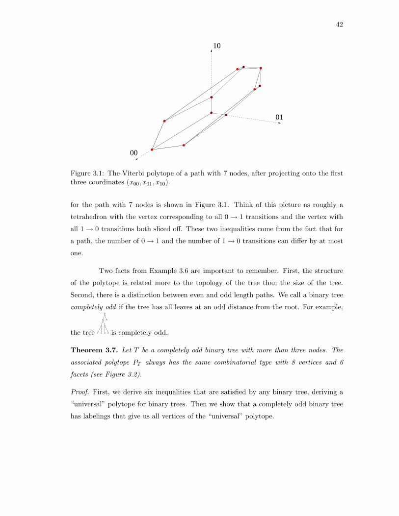
42
10
01
00
Figure 3.1: The Viterbi polytope of a path with 7 nodes, after projecting onto the firstthree coordinates (x00, x01, x10).
for the path with 7 nodes is shown in Figure 3.1. Think of this picture as roughly a
tetrahedron with the vertex corresponding to all 0 → 1 transitions and the vertex with
all 1 → 0 transitions both sliced off. These two inequalities come from the fact that for
a path, the number of 0 → 1 and the number of 1 → 0 transitions can differ by at most
one.
Two facts from Example 3.6 are important to remember. First, the structure
of the polytope is related more to the topology of the tree than the size of the tree.
Second, there is a distinction between even and odd length paths. We call a binary tree
completely odd if the tree has all leaves at an odd distance from the root. For example,
the tree is completely odd.
Theorem 3.7. Let T be a completely odd binary tree with more than three nodes. The
associated polytope PT always has the same combinatorial type with 8 vertices and 6
facets (see Figure 3.2).
Proof. First, we derive six inequalities that are satisfied by any binary tree, deriving a
“universal” polytope for binary trees. Then we show that a completely odd binary tree
has labelings that give us all vertices of the “universal” polytope.

43
Thinking of the polytope space as the log space of the parameters θij, we write
R4 with coordinates b00, b01, b10, b11. Since PT lies in n− 1 times the unit simplex in R
4,
we have b00 + b01 + b10 + b11 = n − 1 and the 4 inequalities bij ≥ 0. We claim that any
binary tree T satisfies two additional inequalities
b00 − b01
2+ b10 ≤
n + 1
2, (3.2)
b11 − b10
2+ b01 ≤
n + 1
2. (3.3)
We prove (3.2), the second inequality follows by interchanging 1 and 0.
Fix a labeling of the binary tree. We claim that the left hand side of (3.2)
counts the net number of zeros that are “created” while moving down the tree, that is,
it counts the number of leaves that are zero minus one if the root is labeled zero. Pick a
non-leaf of the tree which is labeled “0”. It has two children. If both are “0”, then this
node contributes 2 to b00−b01. If both are “1”, then this node contributes -2 to b00−b01.
If one is “0” and one is “1”, then the node doesn’t contribute. We think of a “0” node
with two “0” children as having created a new zero and a “0” node with two “1” children
as having deleted a zero. Therefore we see that the term (b00 − b01)/2 counts the net
number of zeros created as children of “0” nodes. Similarly, if a non-leaf is labeled “1”,
then its contribution to b10 counts the number of new zeros in the children.
Since there are n+12 leaves in a binary tree, there can be at most n+1
2 zeros
created, so (3.2) holds. Notice that the labelings that lie on this facet are exactly those
with a one at the root and all zeros at the leaves.
These six inequalities and the equality b00 + b01 + b10 + b11 = n − 1 define a
three dimensional polytope in R4. It is straightforward to compute that there are eight
vertices of this polytope:
(n − 1, 0, 0, 0), (n − 3, 0, 2, 0)(
n − 3
2,n + 1
2, 0, 0
)
,
(
0,2n
3,n − 3
3, 0
)
(
0,n − 3
3,2n
3, 0
)
,
(
0, 0,n + 1
2,n − 3
2
)
(0, 2, 0, n − 3), (0, 0, 0, n − 1)

44
Six of these vertices occur in any binary tree: a tree with all zeros gives the (n−1, 0, 0, 0)
vertex, a tree with a one at the root and zeros elsewhere gives (n− 3, 0, 2, 0), and a tree
with ones at the leaves and zeros elsewhere gives (n−32 , n+1
2 , 0, 0). Interchanging 1 and
0 gives three more vertices. However, the remaining two vertices aren’t obtained by all
binary trees.
The vertex (0, n−33 , 2n
3 , 0) lies on the facet defined by (3.2), so we know it must
have a one at the root, all zeros at the leaves, and the labels must alternate going down
the tree since there are no zero to zero or one to one transitions. This means that this
vertex is representable by a labeled tree if and only if the tree has all leaves at an odd
depth from the root. Notice that this implies that n must be divisible by 3 for the tree
to be completely odd. Finally, if n > 3 is odd and divisible by 3, then n ≥ 9 and one
checks that the eight vertices are distinct.
See Figure 3.2 for a picture of the polytope and a Schlegel diagram with de-
scriptions of the labelings on the facets and at the vertices.
In the case where T is binary but not completely odd, the polytope shares 6
vertices with this universal polytope, but the remaining 2 vertices are either not integral
or not realizable. However, the polytope still shares much of the boundary with the
universal polytope, so it is perhaps realistic to expect that the polytope for a general
binary tree behaves well. Table 3.3 shows data from computations for all binary trees
with at most 23 nodes. The maximum number of vertices of PT appears to grow very
slowly with the size of the tree.
Although binary trees seem to generally have polytopes with few vertices, ar-
bitrary trees are not so nice. For example, Figure 3.3 shows a tree with 15 nodes that
has a polytope with 34 vertices.
Table 3.4 shows data for all trees on at most 15 nodes. It appears that the
maximum number of vertices for the polytope of an arbitrary tree of size n grows ap-
proximately as 2n. Notice that the tree with all leaves at depth 1 has PT a tetrahedron,
giving the unique minimum number, 4, of vertices for all trees.
Conjecture 3.8. There is a bound on the number of vertices of PT if T is a binary tree.
However, for an arbitrary tree, the number of vertices of PT is unbounded.
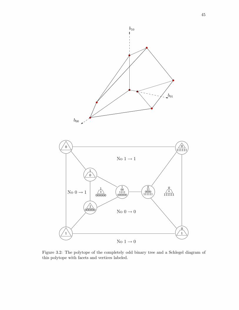
45
0
000000
1*
1
1000000
0111111
0
0*
111111
1 10
011
0000111111000000
1111001
b10
b01
No 0 → 1
No 1 → 1
No 0 → 0
No 1 → 0
b00
Figure 3.2: The polytope of the completely odd binary tree and a Schlegel diagram ofthis polytope with facets and vertices labeled.
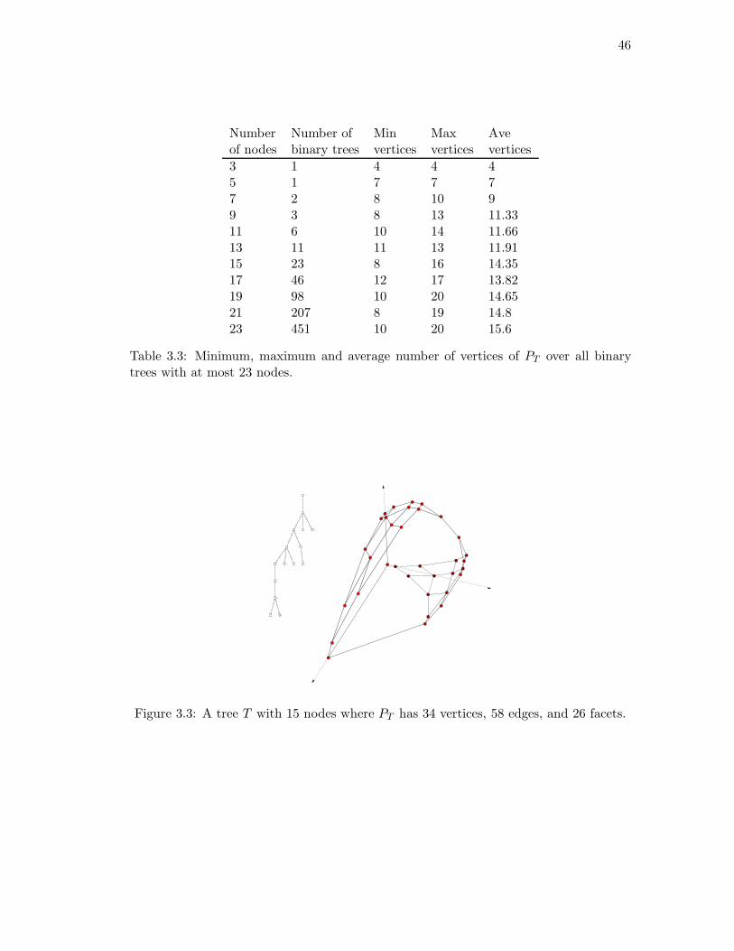
46
Number Number of Min Max Aveof nodes binary trees vertices vertices vertices
3 1 4 4 45 1 7 7 77 2 8 10 99 3 8 13 11.3311 6 10 14 11.6613 11 11 13 11.9115 23 8 16 14.3517 46 12 17 13.8219 98 10 20 14.6521 207 8 19 14.823 451 10 20 15.6
Table 3.3: Minimum, maximum and average number of vertices of PT over all binarytrees with at most 23 nodes.
Figure 3.3: A tree T with 15 nodes where PT has 34 vertices, 58 edges, and 26 facets.

47
Number Number of Min Max Aveof nodes trees vertices vertices vertices
3 2 4 7 5.54 4 4 8 75 9 4 11 86 20 4 14 9.77 48 4 15 10.758 115 4 20 12.599 286 4 21 13.6710 719 4 22 15.4211 1842 4 25 16.6012 4766 4 28 18.313 12486 4 31 19.514 32973 4 32 19.7515 87811 4 34 22.6
Table 3.4: Minimum, maximum and average number of vertices of PT over all trees withat most 15 nodes
We conclude with a description of an algorithm to quickly compute PT . Notice
that the naive method involves taking the convex hull of 2n points, but this can certainly
be improved, since there are many duplicates. The polytope propagation algorithm of
[71] can be used to calculate PT in polynomial time in the number of nodes. This
powerful algorithm can be used to perform parametric inference for many statistical
models of interest to computational biologists. In our case, the algorithm depends on
the observation that PT can be rewritten roughly as the Minkowski sum of PT1 and PT2 ,
where T1 and T2 are the left and right subtrees of the root (after splitting into 8 subcases
depending on the labels of the root and its children). This can be applied recursively
down the tree to give a polynomial time algorithm.
48
Chapter 4
Tree construction using singular
value decomposition
In this chapter, we present a new, statistically consistent algorithm for phyloge-
netic tree construction that uses the algebraic theory of statistical phylogenetic models
as introduced in Section 1.4 and studied in Chapter 3. Our basic tool is Singular Value
Decomposition (SVD) from numerical linear algebra.
Starting with an alignment of n DNA sequences, we show that SVD allows us
to quickly decide whether a split of the taxa occurs in their phylogenetic tree, assuming
only that evolution follows a tree Markov model. Using this fact, we have developed an
algorithm to construct a phylogenetic tree by computing only O(n2) SVDs.
We have implemented this algorithm in C++ using the SVDLIBC library (avail-
able at http://tedlab.mit.edu/∼dr/SVDLIBC/) and have done extensive testing with
simulated and real data. The algorithm is fast in practice on trees with 20–30 taxa.
We begin by describing the general Markov model and then show how to flatten
the joint probability distribution along a partition of the leaves in the tree. We give rank
conditions for the resulting matrix; most notably, we give a set of new rank conditions
that are satisfied by non-splits in the tree. Armed with these rank conditions, we present
the tree-building algorithm, using SVD to calculate how close a matrix is to a certain
rank. Finally, we give experimental results on the behavior of the algorithm with both
simulated and real-life (ENCODE) data. The material in this chapter comes from the
49
book chapter [44].
4.1 The general Markov model
We assume that evolution follows a tree Markov model, as introduced in Section 1.4,
with evolution acting independently at different sites of the genome. We do not assume
that the transition matrices for the model are stochastic. Furthermore, we do not assume
the existence of a global rate matrix.
This model is called the general Markov model. It is a more general model than
any in the Felsenstein hierarchy [73, pg. 154]. The main results in this chapter therefore
hold no matter what model of evolution one works with.
Under the general dogma that statistical models are algebraic varieties, the
polynomials (called “phylogenetic invariants”) defining the varieties are of great interest.
Phylogenetic invariants have been studied extensively since [59, 22]. Linear invariants for
the Jukes–Cantor model have been used to infer phylogenies on four and five taxa; see
[85]. Sturmfels and Sullivant finished the classification of the invariants for group-based
models [97]; see [21] for an application of these invariants for constructing trees on four
taxa. Invariants for the general Markov model have been studied in [2, 3].
The main problem with invariants is that there are exponentially many poly-
nomials in exponentially many variables to test on exponentially many trees. Because
of this, they are currently considered impractical by many and have only been applied
to small problems. However, we solve the problem of this combinatorial explosion by
only concentrating on invariants which are given by rank conditions on certain matrices,
called “flattenings”.
4.2 Flattenings and rank conditions
Recall that a split {A,B} in a tree is a partition of the leaves obtained by removing an
edge of the tree. We will say that {A,B} is a partition of the set of leaves if it is not
necessarily a split but merely a disjoint partition of the set of leaves into two sets.
Throughout, all trees will be assumed to be binary with n leaves. We let m
50
denote the number of states in the alphabet Σ. Usually m = 4 and Σ = {A,C,G, T}
or m = 2 and Σ = {0, 1}. We will write the joint probabilities of an observation on the
leaves as pi1...in . That is, pi1...in is the probability that leaf j is observed to be in state
ij for all j ∈ {1, . . . , n}. We write P for the entire probability distribution.
Although the descriptions of tree-based models in this book all deal with rooted
trees, we will mostly consider unrooted tree models, which are equivalent to them for
the general Markov model; see [3] for details on this technical point. Our tree-building
algorithm constructs an unrooted tree, additional methods would be required to find the
root.
Definition 4.1. A flattening along a partition {A,B} is the m|A| by m|B| matrix where
the rows are indexed by the possible states for the leaves in A and the columns are
indexed by the possible states for the leaves in B. The entries of this matrix are given by
the joint probabilities of observing the given pattern at the leaves. We write FlatA,B(P )
for this matrix.
Example 4.2 (Flattening a partition on 4 taxa). Let T be a tree with 4 leaves and
let m = 4, Σ = {A,C,G,T}. The partition {1, 3}, {2, 4} flattens to the 16 × 16 matrix
Flat{1,3},{2,4}(P ) where the rows are indexed by bases of taxa 1 and 3 and the columns
by bases of taxa 2 and 4:
Flat{1,3},{2,4}(P ) =
AA AC AG AT CA CC . . .
AA pAAAA pAAAC pAAAG pAAAT pACAA pACAC . . .
AC pAACA pAACC pAACG pAACT pACCA pACCC . . .
AG pAAGA pAAGC pAAGG pAAGT pACGA pACGC . . .
AT pAATA pAATC pAATG pAATT pACTA pACTC . . .
CA pCAAA pCAAC pCAAG pCAAT pCCAA pCCAC . . ....
......
......
......
...
.
Next we define a measure of how close a general partition of the leaves is to
being a split. If A is a subset of the leaves of T , we let TA be the subtree induced by the
leaves in A. That is, TA is the minimal set of edges needed to connect the leaves in A.
Definition 4.3. Suppose that {A,B} is a partition of [n]. The distance between the
51
partition {A,B} and the nearest split, written e(A,B), is the number of edges that occur
in TA ∩ TB .
Notice that e(A,B) = 0 exactly when {A,B} is a split. Thus e(A,B) gives a
measure of how close {A,B} is to being a split.
Consider TA∩TB as a subtree of TA. Color the nodes in TA∩TB red, the nodes
in TA \(TA∩TB) blue. Say that a node is monochromatic if it and all of its neighbors are
of the same color. We let mono(A) be the number of monochromatic red nodes. That
is:
Definition 4.4. Define mono(A) as the number of nodes in TA ∩ TB that do not have
a node in TA \ (TA ∩ TB) as a neighbor.
See Figure 4.1 for an example of e(A,B) and mono(A). Our main theorem ties
together how close a partition is to being a split with the rank of the flattening associated
to that partition.
Theorem 4.5. Let {A,B} be a partition of [n], let T be a binary, unrooted tree with
leaves labeled by [n], and assume that the joint probability distribution P comes from a
Markov model on T with an alphabet with m letters. Let
P(A,B) = min (e(A,B) + 1 − mono(A), e(A,B) + 1 − mono(B), |A|, |B|) . (4.1)
Then the generic rank of the flattening FlatA,B(P ) is given by mP(A,B).
Proof. We claim that FlatA,B(P ) can be thought of as the joint distribution for a simple
graphical model. Pick all the nodes that are shared by the induced subtrees for A and
B: call this set R. If R is empty, then {A,B} is a split; in that case let R be one of
the vertices of the edge separating A and B. Notice that |R| = e(A,B) + 1. Think
of these vertices as a single hidden random variable, which we will also call R, with
m|R| = me(A,B)+1 states. Group the states of the nodes in A together into one m|A|-
state observed random variable; similarly the nodes in B are grouped into a m|B|-state
random variable. Then create the graphical model with one hidden m|R|-state random
variable and two descendent observed variables with m|A| and m|B| states. Notice that
FlatA,B(P ) is the joint distribution for this model. See Figure 4.1 for an example.
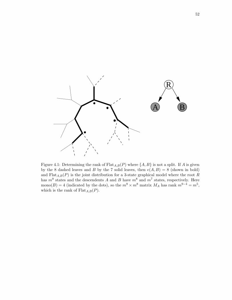
52
��
����
��
��
A
R
B
Figure 4.1: Determining the rank of FlatA,B(P ) where {A,B} is not a split. If A is givenby the 8 dashed leaves and B by the 7 solid leaves, then e(A,B) = 8 (shown in bold)and FlatA,B(P ) is the joint distribution for a 3-state graphical model where the root Rhas m9 states and the descendents A and B have m8 and m7 states, respectively. Heremono(B) = 4 (indicated by the dots), so the m9 ×m8 matrix MA has rank m9−4 = m5,which is the rank of FlatA,B(P ).
53
Furthermore, the distribution for this simplified model factors as
FlatA,B(P ) = MTA diag(π(R))MB (4.2)
where π(R) is the distribution of R and MA and MB are the m|R|×m|A| and m|R|×m|B|
transition matrices. That is, the (i, j)th entry of MA is the probability of transitioning
from state i at the root R to state j at A.
To say the tree distribution factors as (4.2) just means that
Prob(A = i, B = j) =∑
k
Prob(R = k) Prob(A = i | R = k) Prob(B = j | R = k).
Notice that all of the terms in this expression can be written as polynomials in
the edge parameters (after choosing a rooting). Therefore the rank of FlatA,B(P ) is at
most mmin(|R|,|A|,|B|).
However, the matrices in this factorization do not necessarily have full rank.
For example, if one of the nodes in R has only neighbors that are also in R, then the
m|R|×m|A| transition matrices from R to A have many rows that are the same, since the
transition from a state of R to a state of A does not depend on the value of this one node.
More generally, if a node of R has no neighbors in TA \ (TA ∩TB), then the entries of the
transition matrix MA do not depend on the value of this node. But the entries do depend
on the values of all other nodes of R (that is, those with neighbors in TA \ (TA ∩ TB)).
So R really behaves like a model with m|R|−mono(A) states on the transition to A and
m|R|−mono(B) states for the transition to B. There are enough parameters so that after
canceling out these equal rows, all other rows are linearly independent. Therefore, the
rank of MA is min(
m|R|−mono(A),m|A|)
(and similarly for MB).
Remark 4.6. We note that P(A,B) is related to the parsimony score for the tree with
leaves in A in state 0 and leaves in B in state 1. First notice that all the nodes in
TA \ (TA ∩ TB) need to be in state 0 and the nodes in TB \ (TA ∩ TB) need to be in state
1 to obtain a parsimonious tree. Therefore, we are just left with the nodes in TA ∩TB to
decide. If we set all the nodes in TA ∩TB to be in state 1, then e(A,B)+1−mono(A) is
the parsimony score, since this quantity is the number of nodes of TA ∩ TB that have a
node in TA \ (TA ∩TB) as a neighbor. The case where the nodes in TA∩TB are in state 0

54
gives parsimony score e(A,B) + 1−mono(B). In many cases, one of these two labelings
is the most parsiminous. However, there are trees which have a parsimony score which
is lower than P(A,B). For example, trees with large clusters of monochromatic nodes
for both A and B will tend to have low parsimony scores but relatively large P(A,B).
Theorem 4.5 gives rise to a well-known corollary upon noticing that if {A,B}
is a split, then e(A,B) = 0 (see [3], for example).
Corollary 4.7. If {A,B} is a split in the tree, the generic rank of FlatA,B(P ) is m.
A partial converse of Corollary 4.7 will be used later.
Corollary 4.8. If {A,B} is not a split in the tree, and we have |A|, |B| ≥ 2 then the
generic rank of FlatA,B(P ) is at least m2.
Proof. Since we have |A|, |B| ≥ 2, we must show that the two other exponents in (4.1)
are at least 2. That is, we have to show that e(A,B) + 1 − mono(A) ≥ 2 (the case for
B is symmetric). This term counts the number of nodes in TA ∩ TB that are directly
connected to a part of TA outside of TA ∩ TB. Since {A,B} is not a split, we know that
|TA ∩ TB | = e(A,B) + 1 ≥ 2. Consider TA ∩ TB as a subtree with at least 2 nodes of TA.
The only way for all but one of these nodes to be isolated from the rest of the tree is to
have the two consist of a leaf and its parent. However, this is impossible since {A,B} is
a disjoint partition of the set of leaves, so TA ∩ TB contains no leaves.
Example 4.9. In Example 4.2, the 16 × 16 matrix Flat{1,3},{2,4}(P ) has rank 4 if the
split {{1, 3}, {2, 4}} occurs in the tree, otherwise, it has rank 16.
In fact, if m = 2, it has recently been shown [4] that the rank conditions in
Corollary 4.7 generate the ideal of invariants for the general Markov model. However,
they do not suffice if m = 4, since in that case a polynomial of degree 9 lies in the ideal
of invariants (see [95, 51]) but this polynomial is not generated by the degree 5 rank
conditions (see [60]).
4.3 Singular value decomposition
Singular Value Decomposition provides a method to compute the distance between a
matrix and the nearest rank k matrix. In this section, we briefly introduce the basic
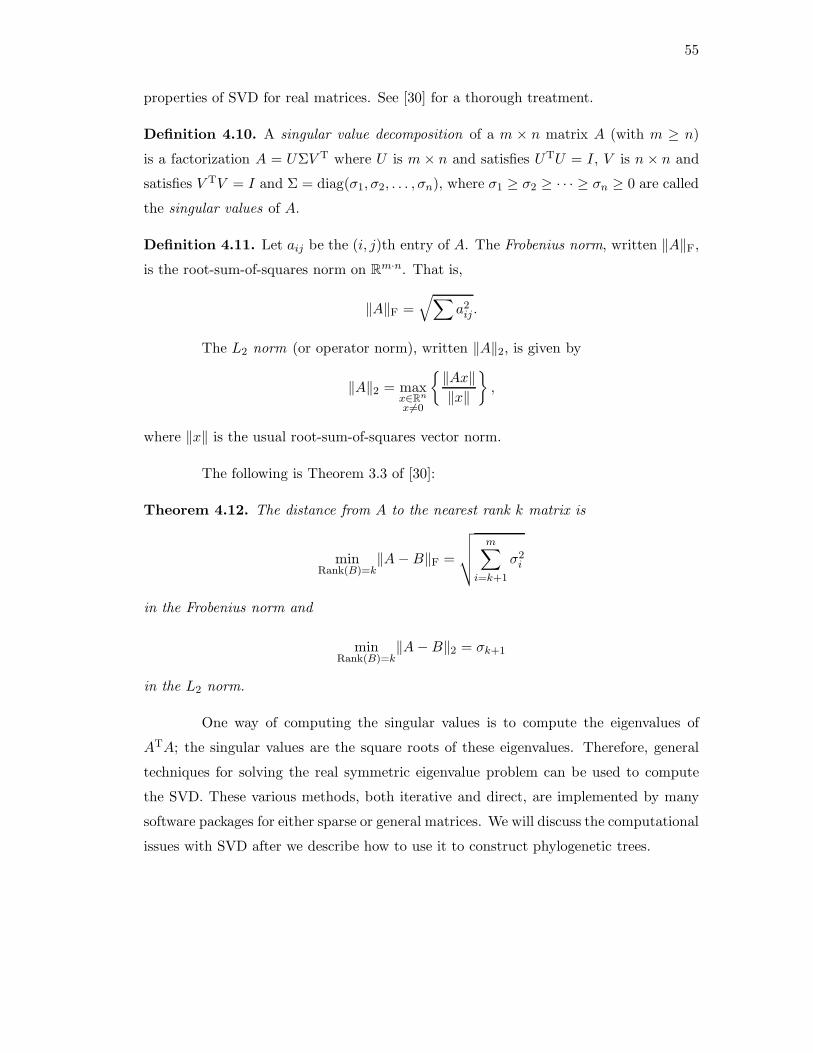
55
properties of SVD for real matrices. See [30] for a thorough treatment.
Definition 4.10. A singular value decomposition of a m × n matrix A (with m ≥ n)
is a factorization A = UΣV T where U is m × n and satisfies UTU = I, V is n × n and
satisfies V TV = I and Σ = diag(σ1, σ2, . . . , σn), where σ1 ≥ σ2 ≥ · · · ≥ σn ≥ 0 are called
the singular values of A.
Definition 4.11. Let aij be the (i, j)th entry of A. The Frobenius norm, written ‖A‖F,
is the root-sum-of-squares norm on Rm·n. That is,
‖A‖F =√
∑
a2ij .
The L2 norm (or operator norm), written ‖A‖2, is given by
‖A‖2 = maxx∈R
n
x 6=0
{
‖Ax‖
‖x‖
}
,
where ‖x‖ is the usual root-sum-of-squares vector norm.
The following is Theorem 3.3 of [30]:
Theorem 4.12. The distance from A to the nearest rank k matrix is
minRank(B)=k
‖A − B‖F =
√
√
√
√
m∑
i=k+1
σ2i
in the Frobenius norm and
minRank(B)=k
‖A − B‖2 = σk+1
in the L2 norm.
One way of computing the singular values is to compute the eigenvalues of
ATA; the singular values are the square roots of these eigenvalues. Therefore, general
techniques for solving the real symmetric eigenvalue problem can be used to compute
the SVD. These various methods, both iterative and direct, are implemented by many
software packages for either sparse or general matrices. We will discuss the computational
issues with SVD after we describe how to use it to construct phylogenetic trees.

56
4.4 Tree-construction algorithm
Now that we know how to tell how close a matrix is to being of a certain rank, we can test
whether a given split comes from the underlying tree or not by using the SVD to tell how
close a flattening matrix is to being rank m. However, since there are exponentially many
possible splits, we must carefully search through this space. Following a suggestion by S.
Snir, we do this by building the tree bottom up, at each step joining cherries together,
in a method reminiscent of neighbor-joining.
It is an interesting open question whether the additional information in Theo-
rem 4.5 about non-splits that are almost splits can be harnessed to produce an improved
algorithm.
Algorithm 4.13 (Tree construction with SVD).
Input: A multiple alignment of genomic data from n species, from the alphabet Σ with
m states.
Output: An unrooted binary tree with n leaves labeled by the species.
Initialization: Compute empirical probabilities pi1...in . That is, count occurrences of
each possible column of the alignment, ignoring columns with characters not in Σ. Store
the results in a sparse format.
Loop: For k from n down to 4, perform the following steps.
For each of the(k2
)
pairs of species compute the SVD for the split {{pair},
{other k − 2 species}}. Pick the pair whose flattening is closest to rank m according to
the Frobenius norm and join this pair together in the tree. That is, consider this pair as
a single element when picking pairs at the next step.
Proposition 4.14. Algorithm 4.13 runs in time O(n3L4) for an input of length L for
n species.
Proof. Notice that although each flattening is of exponential size (i.e., of size m|A|×m|B|),
these matrices must be very sparse. If an alignment is of length L, at most L entries
of the flattening are non-zero. Furthermore, while constructing the flattening, we can
throw out all rows and columns which consist of all zeros. This operation does not take
any additional time beyond the O(nL) time it takes to construct the flattening and it
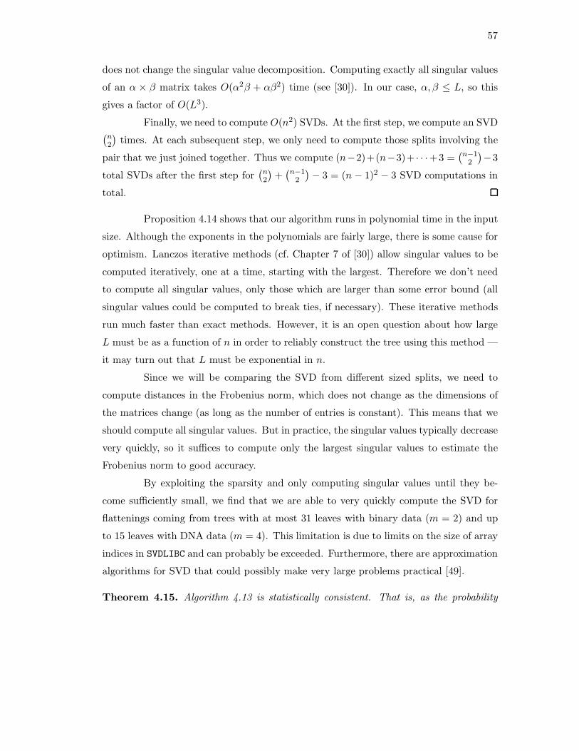
57
does not change the singular value decomposition. Computing exactly all singular values
of an α × β matrix takes O(α2β + αβ2) time (see [30]). In our case, α, β ≤ L, so this
gives a factor of O(L3).
Finally, we need to compute O(n2) SVDs. At the first step, we compute an SVD(n2
)
times. At each subsequent step, we only need to compute those splits involving the
pair that we just joined together. Thus we compute (n−2)+(n−3)+ · · ·+3 =(
n−12
)
−3
total SVDs after the first step for(n2
)
+(n−1
2
)
− 3 = (n − 1)2 − 3 SVD computations in
total.
Proposition 4.14 shows that our algorithm runs in polynomial time in the input
size. Although the exponents in the polynomials are fairly large, there is some cause for
optimism. Lanczos iterative methods (cf. Chapter 7 of [30]) allow singular values to be
computed iteratively, one at a time, starting with the largest. Therefore we don’t need
to compute all singular values, only those which are larger than some error bound (all
singular values could be computed to break ties, if necessary). These iterative methods
run much faster than exact methods. However, it is an open question about how large
L must be as a function of n in order to reliably construct the tree using this method —
it may turn out that L must be exponential in n.
Since we will be comparing the SVD from different sized splits, we need to
compute distances in the Frobenius norm, which does not change as the dimensions of
the matrices change (as long as the number of entries is constant). This means that we
should compute all singular values. But in practice, the singular values typically decrease
very quickly, so it suffices to compute only the largest singular values to estimate the
Frobenius norm to good accuracy.
By exploiting the sparsity and only computing singular values until they be-
come sufficiently small, we find that we are able to very quickly compute the SVD for
flattenings coming from trees with at most 31 leaves with binary data (m = 2) and up
to 15 leaves with DNA data (m = 4). This limitation is due to limits on the size of array
indices in SVDLIBC and can probably be exceeded. Furthermore, there are approximation
algorithms for SVD that could possibly make very large problems practical [49].
Theorem 4.15. Algorithm 4.13 is statistically consistent. That is, as the probability
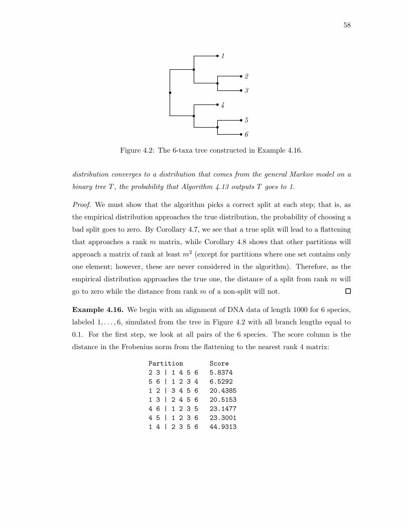
58
b
b
b1
b
b2
b3
b
b4
b
b5
b6
Figure 4.2: The 6-taxa tree constructed in Example 4.16.
distribution converges to a distribution that comes from the general Markov model on a
binary tree T , the probability that Algorithm 4.13 outputs T goes to 1.
Proof. We must show that the algorithm picks a correct split at each step; that is, as
the empirical distribution approaches the true distribution, the probability of choosing a
bad split goes to zero. By Corollary 4.7, we see that a true split will lead to a flattening
that approaches a rank m matrix, while Corollary 4.8 shows that other partitions will
approach a matrix of rank at least m2 (except for partitions where one set contains only
one element; however, these are never considered in the algorithm). Therefore, as the
empirical distribution approaches the true one, the distance of a split from rank m will
go to zero while the distance from rank m of a non-split will not.
Example 4.16. We begin with an alignment of DNA data of length 1000 for 6 species,
labeled 1, . . . , 6, simulated from the tree in Figure 4.2 with all branch lengths equal to
0.1. For the first step, we look at all pairs of the 6 species. The score column is the
distance in the Frobenius norm from the flattening to the nearest rank 4 matrix:
Partition Score
2 3 | 1 4 5 6 5.8374
5 6 | 1 2 3 4 6.5292
1 2 | 3 4 5 6 20.4385
1 3 | 2 4 5 6 20.5153
4 6 | 1 2 3 5 23.1477
4 5 | 1 2 3 6 23.3001
1 4 | 2 3 5 6 44.9313
59
3 4 | 1 2 5 6 52.1283
2 4 | 1 3 5 6 52.6763
1 6 | 2 3 4 5 52.9438
1 5 | 2 3 4 6 53.1727
3 6 | 1 2 4 5 59.5006
3 5 | 1 2 4 6 59.7909
2 6 | 1 3 4 5 59.9546
2 5 | 1 3 4 6 60.3253
picked split 1 4 5 6 | 2 3
tree is 1 4 5 6 (2,3)
After the first step, we see that the split {{2, 3}, {1, 4, 5, 6}} is the best, so
we join nodes 2 and 3 together in the tree and continue. Notice that the scores of the
partitions roughly correspond to how close they are to being splits:
Partition Score
1 2 3 | 4 5 6 5.8534
5 6 | 1 2 3 4 6.5292
4 6 | 1 2 3 5 23.1477
4 5 | 1 2 3 6 23.3001
1 4 | 2 3 5 6 44.9313
2 3 4 | 1 5 6 45.1427
1 6 | 2 3 4 5 52.9438
2 3 6 | 1 4 5 53.0300
1 5 | 2 3 4 6 53.1727
2 3 5 | 1 4 6 53.3838
picked split 1 2 3 | 4 5 6
tree is 4 5 6 (1,(2,3))
After the second step, we join node 1 to the {2, 3} cherry and continue:
Partition Score
5 6 | 1 2 3 4 6.5292
4 6 | 1 2 3 5 23.1477
4 5 | 1 2 3 6 23.3001
picked split 1 2 3 4 | 5 6
tree is 4 (1,(2,3)) (5,6)
Final tree is (4,(1,(2,3)),(5,6))
We have found the last cherry, leaving us with 3 remaining groups which we join together
to form an unrooted tree.
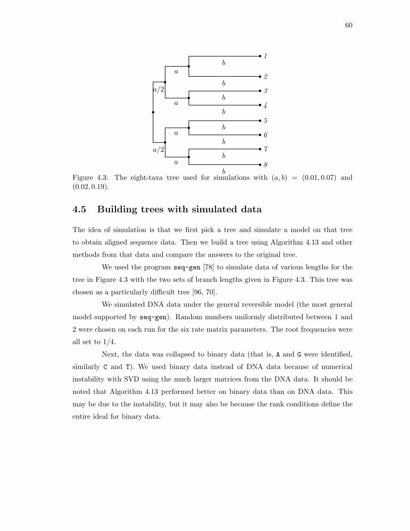
60
b
b
a/2
b
a
b1b
b2b
b
a
b3b
b4b
b
a/2
b
a
b5b
b6b
b
a
b7b
b8b
Figure 4.3: The eight-taxa tree used for simulations with (a, b) = (0.01, 0.07) and(0.02, 0.19).
4.5 Building trees with simulated data
The idea of simulation is that we first pick a tree and simulate a model on that tree
to obtain aligned sequence data. Then we build a tree using Algorithm 4.13 and other
methods from that data and compare the answers to the original tree.
We used the program seq-gen [78] to simulate data of various lengths for the
tree in Figure 4.3 with the two sets of branch lengths given in Figure 4.3. This tree was
chosen as a particularly difficult tree [96, 70].
We simulated DNA data under the general reversible model (the most general
model supported by seq-gen). Random numbers uniformly distributed between 1 and
2 were chosen on each run for the six rate matrix parameters. The root frequencies were
all set to 1/4.
Next, the data was collapsed to binary data (that is, A and G were identified,
similarly C and T). We used binary data instead of DNA data because of numerical
instability with SVD using the much larger matrices from the DNA data. It should be
noted that Algorithm 4.13 performed better on binary data than on DNA data. This
may be due to the instability, but it may also be because the rank conditions define the
entire ideal for binary data.
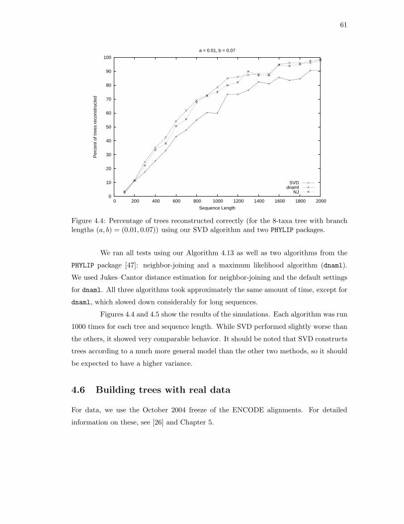
61
0
10
20
30
40
50
60
70
80
90
100
0 200 400 600 800 1000 1200 1400 1600 1800 2000
Per
cent
of t
rees
rec
onst
ruct
ed
Sequence Length
a = 0.01, b = 0.07
SVDdnaml
NJ
Figure 4.4: Percentage of trees reconstructed correctly (for the 8-taxa tree with branchlengths (a, b) = (0.01, 0.07)) using our SVD algorithm and two PHYLIP packages.
We ran all tests using our Algorithm 4.13 as well as two algorithms from the
PHYLIP package [47]: neighbor-joining and a maximum likelihood algorithm (dnaml).
We used Jukes–Cantor distance estimation for neighbor-joining and the default settings
for dnaml. All three algorithms took approximately the same amount of time, except for
dnaml, which slowed down considerably for long sequences.
Figures 4.4 and 4.5 show the results of the simulations. Each algorithm was run
1000 times for each tree and sequence length. While SVD performed slightly worse than
the others, it showed very comparable behavior. It should be noted that SVD constructs
trees according to a much more general model than the other two methods, so it should
be expected to have a higher variance.
4.6 Building trees with real data
For data, we use the October 2004 freeze of the ENCODE alignments. For detailed
information on these, see [26] and Chapter 5.
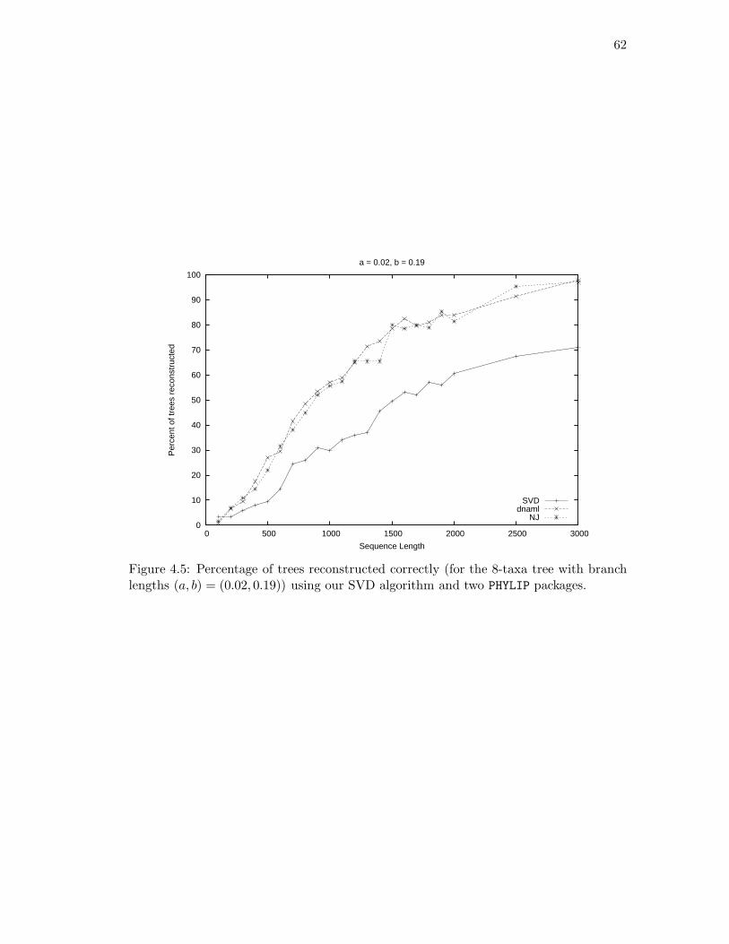
62
0
10
20
30
40
50
60
70
80
90
100
0 500 1000 1500 2000 2500 3000
Per
cent
of t
rees
rec
onst
ruct
ed
Sequence Length
a = 0.02, b = 0.19
SVDdnaml
NJ
Figure 4.5: Percentage of trees reconstructed correctly (for the 8-taxa tree with branchlengths (a, b) = (0.02, 0.19)) using our SVD algorithm and two PHYLIP packages.
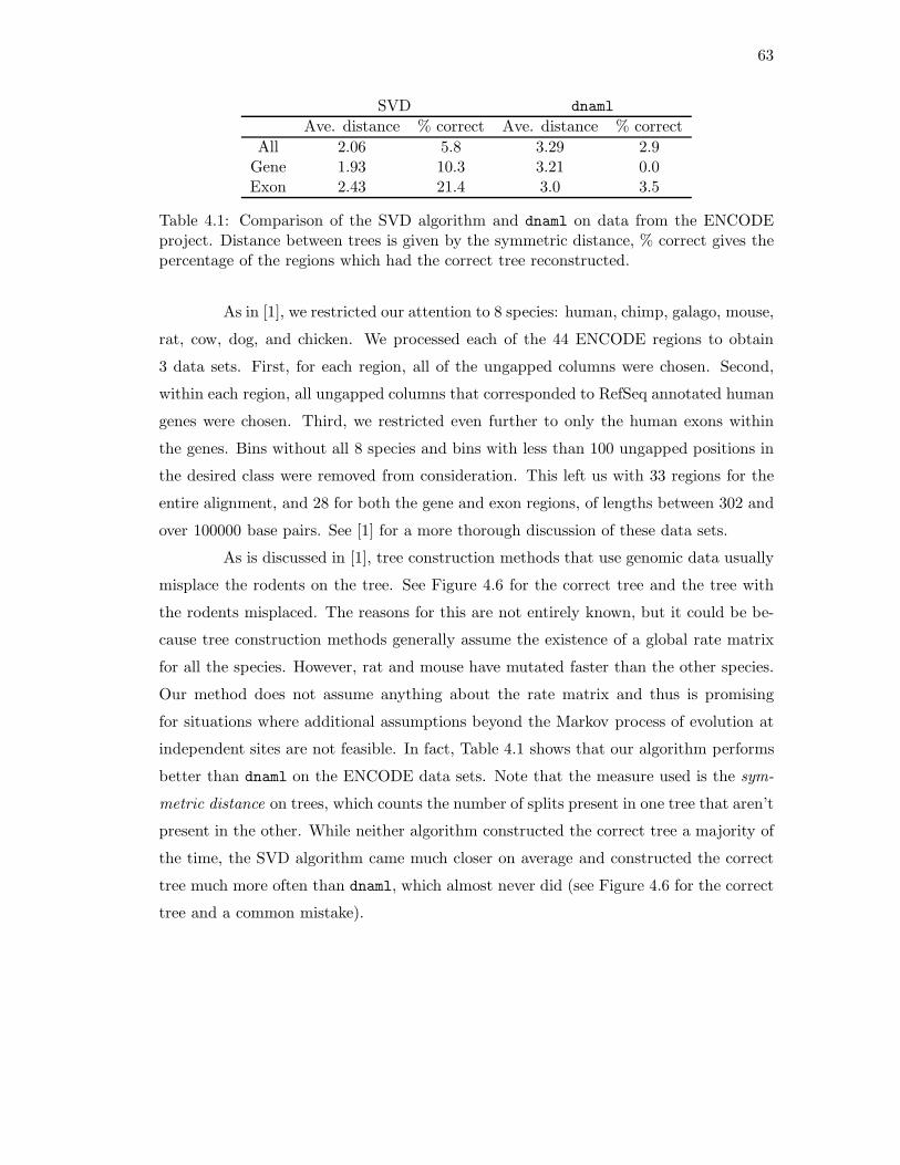
63
SVD dnaml
Ave. distance % correct Ave. distance % correct
All 2.06 5.8 3.29 2.9Gene 1.93 10.3 3.21 0.0Exon 2.43 21.4 3.0 3.5
Table 4.1: Comparison of the SVD algorithm and dnaml on data from the ENCODEproject. Distance between trees is given by the symmetric distance, % correct gives thepercentage of the regions which had the correct tree reconstructed.
As in [1], we restricted our attention to 8 species: human, chimp, galago, mouse,
rat, cow, dog, and chicken. We processed each of the 44 ENCODE regions to obtain
3 data sets. First, for each region, all of the ungapped columns were chosen. Second,
within each region, all ungapped columns that corresponded to RefSeq annotated human
genes were chosen. Third, we restricted even further to only the human exons within
the genes. Bins without all 8 species and bins with less than 100 ungapped positions in
the desired class were removed from consideration. This left us with 33 regions for the
entire alignment, and 28 for both the gene and exon regions, of lengths between 302 and
over 100000 base pairs. See [1] for a more thorough discussion of these data sets.
As is discussed in [1], tree construction methods that use genomic data usually
misplace the rodents on the tree. See Figure 4.6 for the correct tree and the tree with
the rodents misplaced. The reasons for this are not entirely known, but it could be be-
cause tree construction methods generally assume the existence of a global rate matrix
for all the species. However, rat and mouse have mutated faster than the other species.
Our method does not assume anything about the rate matrix and thus is promising
for situations where additional assumptions beyond the Markov process of evolution at
independent sites are not feasible. In fact, Table 4.1 shows that our algorithm performs
better than dnaml on the ENCODE data sets. Note that the measure used is the sym-
metric distance on trees, which counts the number of splits present in one tree that aren’t
present in the other. While neither algorithm constructed the correct tree a majority of
the time, the SVD algorithm came much closer on average and constructed the correct
tree much more often than dnaml, which almost never did (see Figure 4.6 for the correct
tree and a common mistake).
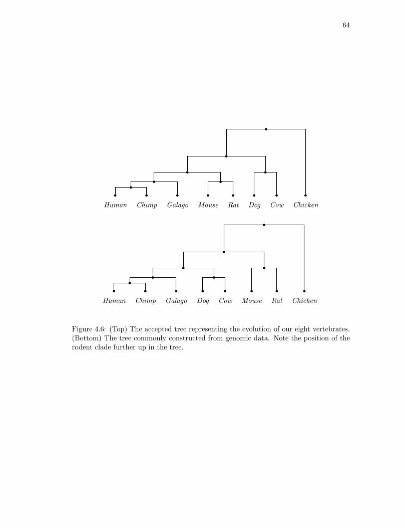
64
b
b
b
b
b
b
Human
b
Chimp
b
Galago
b
b
Mouse
b
Rat
b
b
Dog
b
Cow
b
Chicken
b
b
b
b
b
b
Human
b
Chimp
b
Galago
b
b
Dog
b
Cow
b
b
Mouse
b
Rat
b
Chicken
Figure 4.6: (Top) The accepted tree representing the evolution of our eight vertebrates.(Bottom) The tree commonly constructed from genomic data. Note the position of therodent clade further up in the tree.

65
Chapter 5
Ultra-conserved elements in
vertebrate and fly genomes
Ultra-conserved elements in an alignment of multiple genomes are consecutive
nucleotides that are in perfect agreement across all the genomes. In this chapter, we
examine ultra-conserved elements in aligned vertebrate and fly genomes. In Section 5.1,
we describe the selected species and alignments. In Section 5.2, we give descriptive
statistics of ultra-conserved elements, and in Section 5.3 we explain their biological rel-
evance. Finally, in Section 5.4 we use the phylogenetic models introduced in Chapter 1
and studied in Chapters 3 and 4 to show that the existence of ultra-conserved elements
is highly improbable in neutrally evolving regions.
The results in this chapter come from a book chapter [40] written with Mathias
Drton and Garmay Leung. Many of our results mirror those of previous studies. How-
ever, these studies have considered long stretches of perfectly conserved regions across
shorter evolutionary distances [14], or aligned regions above some relatively high thresh-
old level of conservation [17, 84, 106]. We have focused on ultra-conserved elements
across larger evolutionary distances. As a result, we have not captured all regions con-
taining high levels of conservation, but have identified only those regions that appear to
be under the most stringent evolutionary constraints.

66
5.1 The data
Our analyses of ultra-conserved elements are based on multiple sequence alignments
produced by MAVID [18]. Prior to the alignment of multiple genomes, homology mappings
(from Mercator [32]) group into bins genomic regions that are anchored together by
neighboring homologous exons. A multiple sequence alignment is then produced for each
of these alignment bins. MAVID is a global multiple alignment program, and therefore
homologous regions with more than one homologous hit to another genome may not be
found aligned together. Table 5.1 shows an example of Mercator’s output for a single
region along with the beginning of the resulting MAVID multiple sequence alignment.
Species Chrom. Start End Alignment
Dog chrX 752057 864487 + A----AACCAAA---------
Chicken chr1 122119382 122708162 − TGCTGAGCTAAAGATCAGGCT
Zebra fish chr9 19018916 19198136 + ------ATGCAACATGCTTCT
Puffer fish chr2 7428614 7525502 + ---TAGATGGCAGACGATGCT
Fugu fish asm1287 21187 82482 + ---TCAAGGG-----------
Table 5.1: Mercator output for a single bin, giving the position and orientation onthe chromosome. Notice that the Fugu fish genome has not been fully assembled intochromosomes.
The vertebrate dataset consists of 10,279 bins over 9 genomes (Table 5.2). A
total of 4,368 bins (42.5%) contain alignments across all 9 species. The evolutionary
relationships among these species (which first diverged about 450 million years ago) are
shown in Figure 5.1. With the exception of the probability calculations in phylogenetic
tree models, our subsequent findings on ultra-conserved elements do not depend on the
form of this tree.
The fruit fly dataset consists of 8 Drosophila genomes (Table 5.3). Of the 3,731
alignment bins, 2,985 (80.0%) contain all 8 species, which reflects the smaller degree of
evolutionary divergence. A phylogenetic tree for these 8 species, which diverged at least
45 million years ago, is shown in Figure 5.2.
The pilot phase of the ENCODE project [26] provides an additional dataset
of vertebrate sequences homologous to 44 regions of the human genome. There are
14 manually selected regions of particular biological interest and 30 randomly selected
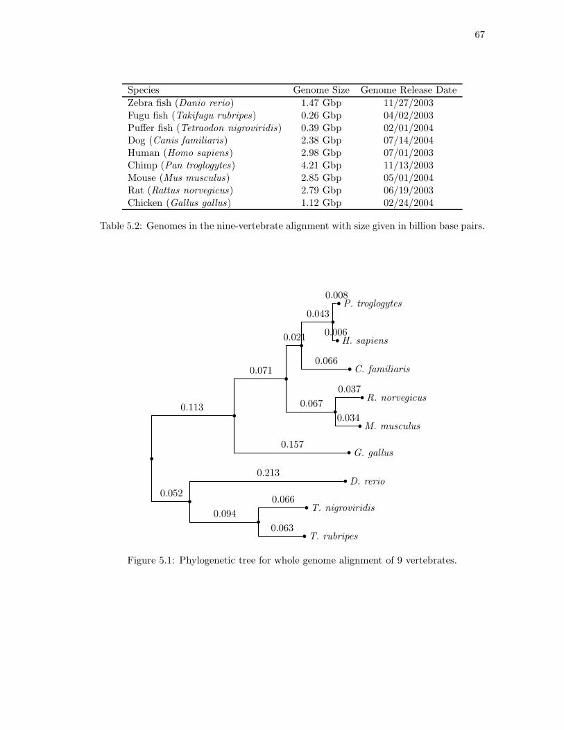
67
Species Genome Size Genome Release Date
Zebra fish (Danio rerio) 1.47 Gbp 11/27/2003Fugu fish (Takifugu rubripes) 0.26 Gbp 04/02/2003Puffer fish (Tetraodon nigroviridis) 0.39 Gbp 02/01/2004Dog (Canis familiaris) 2.38 Gbp 07/14/2004Human (Homo sapiens) 2.98 Gbp 07/01/2003Chimp (Pan troglogytes) 4.21 Gbp 11/13/2003Mouse (Mus musculus) 2.85 Gbp 05/01/2004Rat (Rattus norvegicus) 2.79 Gbp 06/19/2003Chicken (Gallus gallus) 1.12 Gbp 02/24/2004
Table 5.2: Genomes in the nine-vertebrate alignment with size given in billion base pairs.
b
b
0.113
b
0.071
b
0.021
b
0.043
bP. troglogytes0.008
bH. sapiens0.006
bC. familiaris0.066
b
0.067bR. norvegicus
0.037
bM. musculus0.034
bG. gallus0.157
b
0.052
bD. rerio0.213
b
0.094bT. nigroviridis
0.066
bT. rubripes0.063
Figure 5.1: Phylogenetic tree for whole genome alignment of 9 vertebrates.
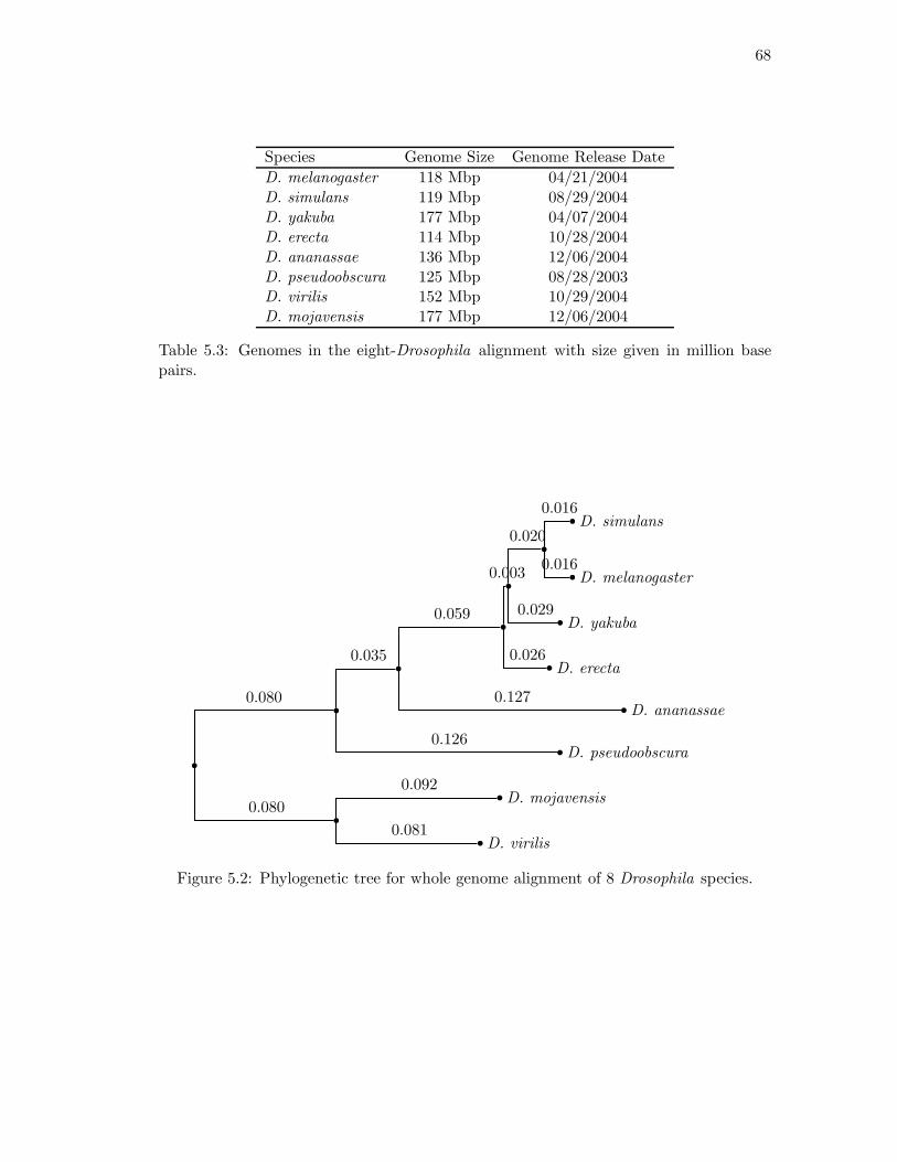
68
Species Genome Size Genome Release Date
D. melanogaster 118 Mbp 04/21/2004D. simulans 119 Mbp 08/29/2004D. yakuba 177 Mbp 04/07/2004D. erecta 114 Mbp 10/28/2004D. ananassae 136 Mbp 12/06/2004D. pseudoobscura 125 Mbp 08/28/2003D. virilis 152 Mbp 10/29/2004D. mojavensis 177 Mbp 12/06/2004
Table 5.3: Genomes in the eight-Drosophila alignment with size given in million basepairs.
b
b
0.080
b
0.035
b
0.059
b
0.003
b
0.020bD. simulans
0.016
bD. melanogaster0.016
bD. yakuba0.029
bD. erecta0.026
bD. ananassae0.127
bD. pseudoobscura0.126
b
0.080bD. mojavensis
0.092
bD. virilis0.081
Figure 5.2: Phylogenetic tree for whole genome alignment of 8 Drosophila species.
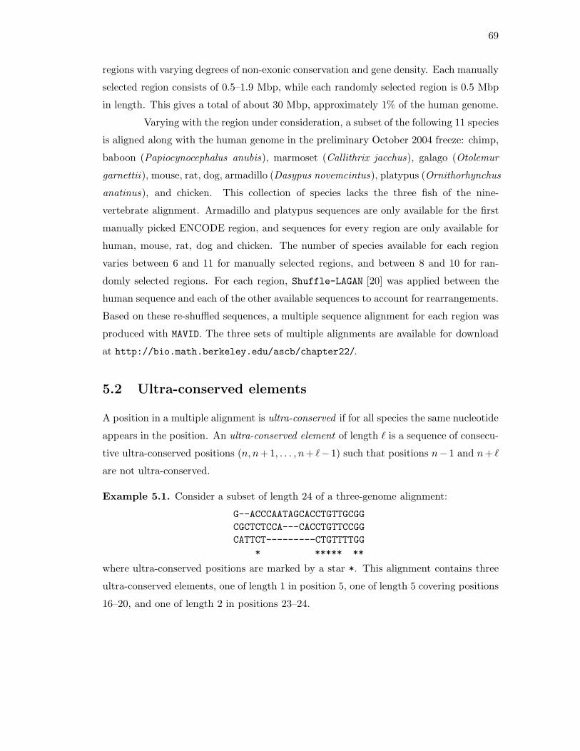
69
regions with varying degrees of non-exonic conservation and gene density. Each manually
selected region consists of 0.5–1.9 Mbp, while each randomly selected region is 0.5 Mbp
in length. This gives a total of about 30 Mbp, approximately 1% of the human genome.
Varying with the region under consideration, a subset of the following 11 species
is aligned along with the human genome in the preliminary October 2004 freeze: chimp,
baboon (Papiocynocephalus anubis), marmoset (Callithrix jacchus), galago (Otolemur
garnettii), mouse, rat, dog, armadillo (Dasypus novemcintus), platypus (Ornithorhynchus
anatinus), and chicken. This collection of species lacks the three fish of the nine-
vertebrate alignment. Armadillo and platypus sequences are only available for the first
manually picked ENCODE region, and sequences for every region are only available for
human, mouse, rat, dog and chicken. The number of species available for each region
varies between 6 and 11 for manually selected regions, and between 8 and 10 for ran-
domly selected regions. For each region, Shuffle-LAGAN [20] was applied between the
human sequence and each of the other available sequences to account for rearrangements.
Based on these re-shuffled sequences, a multiple sequence alignment for each region was
produced with MAVID. The three sets of multiple alignments are available for download
at http://bio.math.berkeley.edu/ascb/chapter22/.
5.2 Ultra-conserved elements
A position in a multiple alignment is ultra-conserved if for all species the same nucleotide
appears in the position. An ultra-conserved element of length ℓ is a sequence of consecu-
tive ultra-conserved positions (n, n+1, . . . , n+ ℓ− 1) such that positions n− 1 and n+ ℓ
are not ultra-conserved.
Example 5.1. Consider a subset of length 24 of a three-genome alignment:
G--ACCCAATAGCACCTGTTGCGG
CGCTCTCCA---CACCTGTTCCGG
CATTCT---------CTGTTTTGG
* ***** **
where ultra-conserved positions are marked by a star *. This alignment contains three
ultra-conserved elements, one of length 1 in position 5, one of length 5 covering positions
16–20, and one of length 2 in positions 23–24.
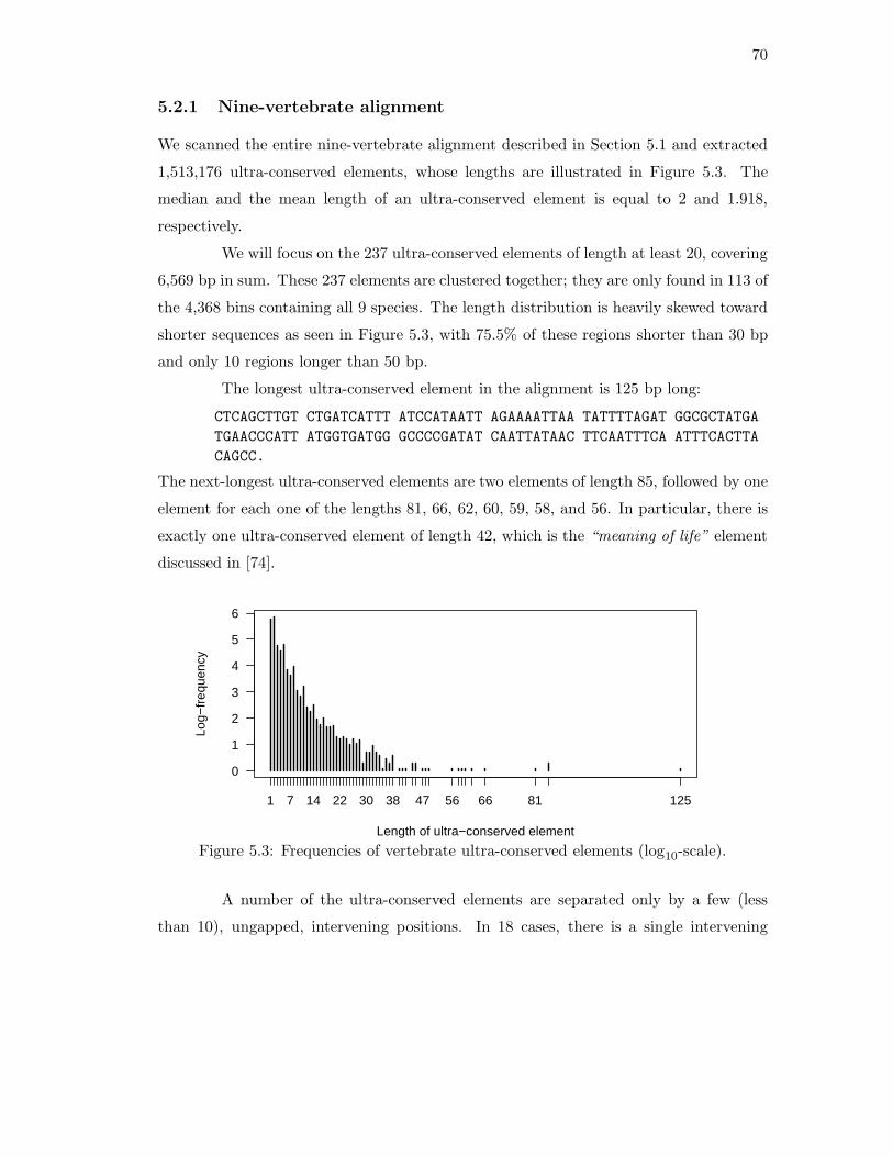
70
5.2.1 Nine-vertebrate alignment
We scanned the entire nine-vertebrate alignment described in Section 5.1 and extracted
1,513,176 ultra-conserved elements, whose lengths are illustrated in Figure 5.3. The
median and the mean length of an ultra-conserved element is equal to 2 and 1.918,
respectively.
We will focus on the 237 ultra-conserved elements of length at least 20, covering
6,569 bp in sum. These 237 elements are clustered together; they are only found in 113 of
the 4,368 bins containing all 9 species. The length distribution is heavily skewed toward
shorter sequences as seen in Figure 5.3, with 75.5% of these regions shorter than 30 bp
and only 10 regions longer than 50 bp.
The longest ultra-conserved element in the alignment is 125 bp long:
CTCAGCTTGT CTGATCATTT ATCCATAATT AGAAAATTAA TATTTTAGAT GGCGCTATGA
TGAACCCATT ATGGTGATGG GCCCCGATAT CAATTATAAC TTCAATTTCA ATTTCACTTA
CAGCC.
The next-longest ultra-conserved elements are two elements of length 85, followed by one
element for each one of the lengths 81, 66, 62, 60, 59, 58, and 56. In particular, there is
exactly one ultra-conserved element of length 42, which is the “meaning of life” element
discussed in [74].
0
1
2
3
4
5
6
Length of ultra−conserved element
Log−
freq
uenc
y
1 7 14 22 30 38 47 56 66 81 125
Figure 5.3: Frequencies of vertebrate ultra-conserved elements (log10-scale).
A number of the ultra-conserved elements are separated only by a few (less
than 10), ungapped, intervening positions. In 18 cases, there is a single intervening

71
position. Typically, these positions are nearly ultra-conserved, and display differences
only between the fish and the other species. Collapsing the ultra-conserved elements
separated by fewer than 10 bases reduces the number of ultra-conserved elements to 209,
increases the base coverage to 6,636 bp, and brings the total number of regions greater
than 50 bp in length to 26.
In the human genome, the GC-ratio (proportion of G and C among all nucleotides)
is 41.0%. The ultra-conserved elements are slightly more AT-rich; for the 237 elements
of length 20 or longer, the GC-ratio is 35.8%. However, GC-content and local sequence
characteristics were not enough to identify ultra-conserved regions using data from only
one genome.
5.2.2 ENCODE alignment
The 44 ENCODE regions contain 139,043 ultra-conserved elements, 524 of which are
longer than 20 bp. These long elements cover 17,823 bp. By base coverage, 73.5% of
the long elements are found in the manually chosen regions. The longest one is in region
ENm012, of length 169 and consists of the DNA sequence:
AAGTGCTTTG TGAGTTTGTC ACCAATGATA ATTTAGATAG AGGCTCATTA CTGAACATCA
CAACACTTTA AAAACCTTTC GCCTTCATAC AGGAGAATAA AGGACTATTT TAATGGCAAG
GTTCTTTTGT GTTCCACTGA AAAATTCAAT CAAGACAAAA CCTCATTGA.
This sequence does not contain a subsequence of length 20 or longer that is ultra-
conserved in the nine-vertebrate alignment, but the 169 bp are also ultra-conserved
in the nine-vertebrate alignment if the three fish are excluded from consideration. The
only overlap between the nine-vertebrate and ENCODE ultra-conserved elements occurs
in the regions ENm012 and ENm005, where there are 3 elements that are extensions of
ultra-conserved elements in the nine-vertebrate alignment.
Table 5.4 shows the number of species aligned in the 44 ENCODE alignments
and the respective five longest ultra-conserved elements that are of length 20 or larger.
Omitted randomly selected regions do not contain any ultra-conserved elements of length
at least 20.
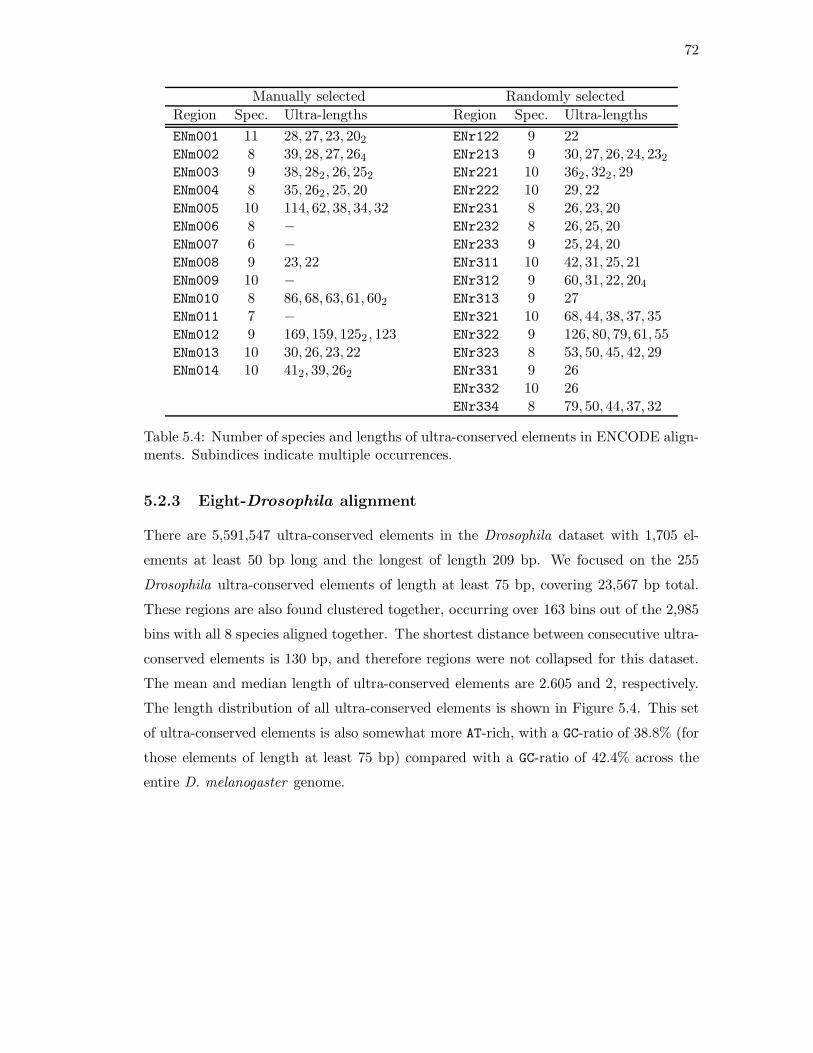
72
Manually selected Randomly selected
Region Spec. Ultra-lengths Region Spec. Ultra-lengths
ENm001 11 28, 27, 23, 202 ENr122 9 22ENm002 8 39, 28, 27, 264 ENr213 9 30, 27, 26, 24, 232
ENm003 9 38, 282, 26, 252 ENr221 10 362, 322, 29ENm004 8 35, 262, 25, 20 ENr222 10 29, 22ENm005 10 114, 62, 38, 34, 32 ENr231 8 26, 23, 20ENm006 8 − ENr232 8 26, 25, 20ENm007 6 − ENr233 9 25, 24, 20ENm008 9 23, 22 ENr311 10 42, 31, 25, 21ENm009 10 − ENr312 9 60, 31, 22, 204
ENm010 8 86, 68, 63, 61, 602 ENr313 9 27ENm011 7 − ENr321 10 68, 44, 38, 37, 35ENm012 9 169, 159, 1252 , 123 ENr322 9 126, 80, 79, 61, 55ENm013 10 30, 26, 23, 22 ENr323 8 53, 50, 45, 42, 29ENm014 10 412, 39, 262 ENr331 9 26
ENr332 10 26ENr334 8 79, 50, 44, 37, 32
Table 5.4: Number of species and lengths of ultra-conserved elements in ENCODE align-ments. Subindices indicate multiple occurrences.
5.2.3 Eight-Drosophila alignment
There are 5,591,547 ultra-conserved elements in the Drosophila dataset with 1,705 el-
ements at least 50 bp long and the longest of length 209 bp. We focused on the 255
Drosophila ultra-conserved elements of length at least 75 bp, covering 23,567 bp total.
These regions are also found clustered together, occurring over 163 bins out of the 2,985
bins with all 8 species aligned together. The shortest distance between consecutive ultra-
conserved elements is 130 bp, and therefore regions were not collapsed for this dataset.
The mean and median length of ultra-conserved elements are 2.605 and 2, respectively.
The length distribution of all ultra-conserved elements is shown in Figure 5.4. This set
of ultra-conserved elements is also somewhat more AT-rich, with a GC-ratio of 38.8% (for
those elements of length at least 75 bp) compared with a GC-ratio of 42.4% across the
entire D. melanogaster genome.

73
0
1
2
3
4
5
6
Length of ultra−conserved element
Log−
freq
uenc
y
1 9 19 30 41 52 63 74 85 96 109 123 137 155 169 192 209
Figure 5.4: Frequencies of Drosophila ultra-conserved elements (log10-scale).
5.3 Biology of ultra-conserved elements
5.3.1 Nine-vertebrate alignment
Using the UCSC genome browser annotations of known genes for the July 2003 (hg16)
release of the human genome, we investigated which ultra-conserved elements overlap
known functional regions. Intragenic regions cover 62.6% of the bases of the 209 col-
lapsed ultra-conserved elements described in Section 5.2.1. However, intragenic coverage
increases to 67.6% for short elements (less than 30 bp) and drops to 56.3% for longer
elements (at least 30 bp), as shown in Figures 5.5(a) and 5.5(b). While shorter ultra-
conserved elements tend to correspond to exons, longer ones are generally associated with
introns and unannotated regions. Nine ultra-conserved elements cover a total of 306 bp
in the intronic regions of POLA, the alpha catalytic subunit of DNA polymerase. Six
other genes are associated with more than 100 bp of ultra-conserved elements. Four of
these genes are transcription factors involved in development (SOX6, FOXP2, DACH1,
TCF7L2 ). In fact, elements near DACH that were highly conserved between human
and mouse and also present in fish species have been shown to be DACH enhancers; see
[68].
Among the 237 uncollapsed ultra-conserved elements of length at least 20, 151
are in intragenic regions of 96 genes. The remaining 86 elements did not overlap any
annotated gene. However, by grouping together elements that have the same upstream
and downstream flanking genes, there are only 27 super-regions to consider, with 51
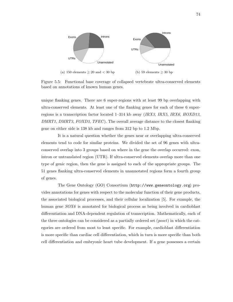
74
IntronsExons
UTRsUnannotated
(a) 150 elements ≥ 20 and < 30 bp
Introns
Exons
UTRs
Unannotated
(b) 59 elements ≥ 30 bp
Figure 5.5: Functional base coverage of collapsed vertebrate ultra-conserved elementsbased on annotations of known human genes.
unique flanking genes. There are 6 super-regions with at least 99 bp overlapping with
ultra-conserved elements. At least one of the flanking genes for each of these 6 super-
regions is a transcription factor located 1–314 kb away (IRX3, IRX5, IRX6, HOXD13,
DMRT1, DMRT3, FOXD3, TFEC ). The overall average distance to the closest flanking
gene on either side is 138 kb and ranges from 312 bp to 1.2 Mbp.
It is a natural question whether the genes near or overlapping ultra-conserved
elements tend to code for similar proteins. We divided the set of 96 genes with ultra-
conserved overlap into 3 groups based on where in the gene the overlap occurred: exon,
intron or untranslated region (UTR). If ultra-conserved elements overlap more than one
type of genic region, then the gene is assigned to each of the appropriate groups. The
51 genes flanking ultra-conserved elements in unannotated regions form a fourth group
of genes.
The Gene Ontology (GO) Consortium (http://www.geneontology.org) pro-
vides annotations for genes with respect to the molecular function of their gene products,
the associated biological processes, and their cellular localization [5]. For example, the
human gene SOX6 is annotated for biological process as being involved in cardioblast
differentiation and DNA-dependent regulation of transcription. Mathematically, each of
the three ontologies can be considered as a partially ordered set (poset) in which the cat-
egories are ordered from most to least specific. For example, cardioblast differentiation
is more specific than cardiac cell differentiation, which in turn is more specific than both
cell differentiation and embryonic heart tube development. If a gene possesses a certain

75
annotation, it must also possess all more general annotations; therefore GO consists of
a map from the set of genes to order ideals in the three posets. We propose that this
mathematical structure is important for analyzing the GO project.
In this study, we only considered molecular function and biological process an-
notations. These annotations are available for 46 of the 54 genes with exonic overlap, for
all of the 28 with intronic overlap, for 14 of the 20 with UTR overlap, and for 30 of the
51 genes flanking unannotated elements. Considering one GO annotation and one of the
4 gene groups at a time, we counted how many of the genes in the group are associated
with the considered annotation. Using counts of how often this annotation occurs among
all proteins found in Release 4.1 of the Uniprot database (http://www.uniprot.org),
we computed a p-value from Fisher’s exact test for independence of association with the
annotation and affiliation with the considered gene group. Annotations associated with
at least 3 genes in a group and with an unadjusted p-value smaller than 3.0 ·10−2 are re-
ported in Table 5.5. DNA-dependent regulation of transcription and transcription factor
activity are found to be enriched in non-exonic ultra-conserved elements, corresponding
to previously reported findings [14, 17, 84, 106]. Conserved exonic elements tend to be
involved in protein modification.
We scanned the human genome for repeated instances of these ultra-conserved
elements and found that 14 of the original 237 elements have at least one other instance
within the human genome. Generally, the repeats are not ultra-conserved except for some
of the seven repeats that are found both between IRX6 and IRX5 and between IRX5
and IRX3 on chromosome 16. These genes belong to a cluster of Iroquois homeobox
genes involved in embryonic pattern formation [75]. These repeated elements include two
32 bp sequences that are perfect reverse complements of each other and two (of lengths 23
bp and 28 bp) that are truncated reverse complements of each other. Overall, there are 5
distinct sequences within 226 bp regions on either side of IRX5 that are perfect reverse
complements of each other. The reverse complements are found in the same relative
order (Figure 5.6). Furthermore, exact copies of the two outermost sequences are found
both between IRX4 and IRX2 and between IRX2 and IRX1 on chromosome 5. Both
of these regions are exactly 226 bp long. The repetition of these short regions and the
conservation of their relative ordering and size suggests a highly specific coordinated
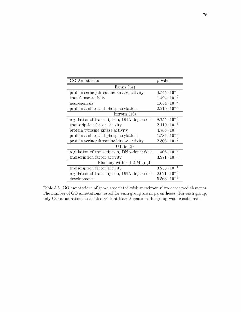
76
GO Annotation p-value
Exons (14)
protein serine/threonine kinase activity 4.545 · 10−3
transferase activity 1.494 · 10−2
neurogenesis 1.654 · 10−2
protein amino acid phosphorylation 2.210 · 10−2
Introns (10)
regulation of transcription, DNA-dependent 8.755 · 10−4
transcription factor activity 2.110 · 10−3
protein tyrosine kinase activity 4.785 · 10−3
protein amino acid phosphorylation 1.584 · 10−2
protein serine/threonine kinase activity 2.806 · 10−2
UTRs (3)
regulation of transcription, DNA-dependent 1.403 · 10−4
transcription factor activity 3.971 · 10−3
Flanking within 1.2 Mbp (4)
transcription factor activity 3.255 · 10−11
regulation of transcription, DNA-dependent 2.021 · 10−8
development 5.566 · 10−3
Table 5.5: GO annotations of genes associated with vertebrate ultra-conserved elements.The number of GO annotations tested for each group are in parentheses. For each group,only GO annotations associated with at least 3 genes in the group were considered.
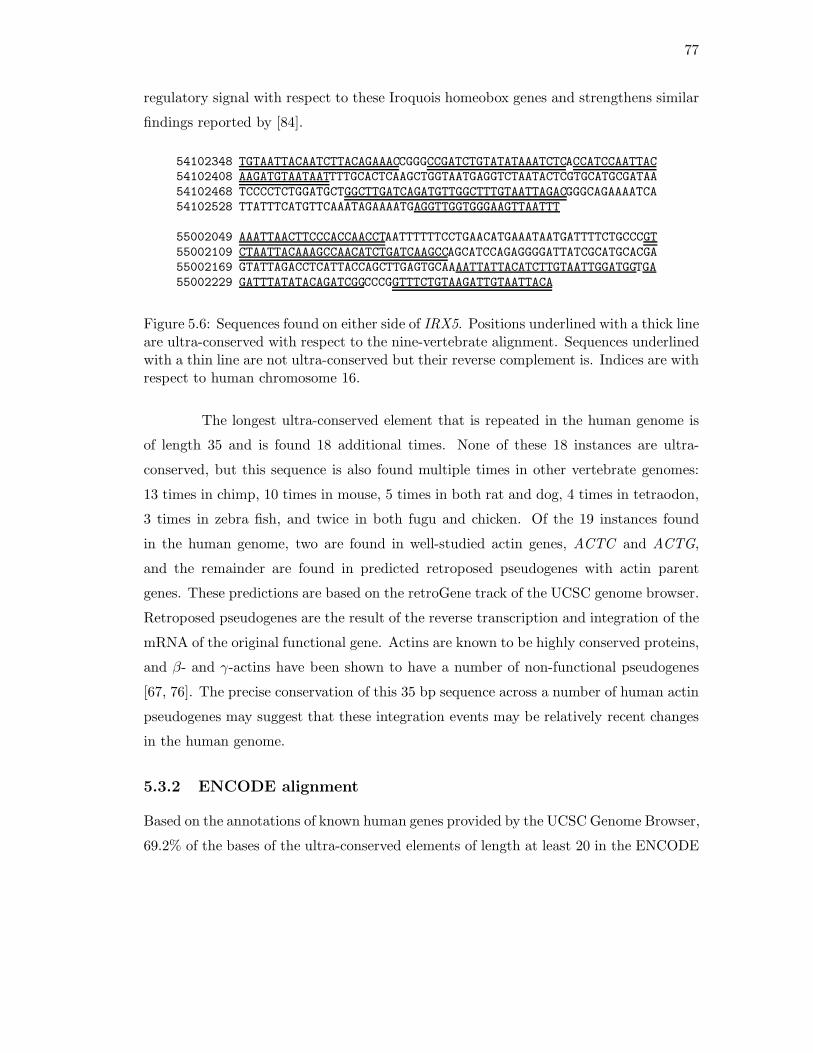
77
regulatory signal with respect to these Iroquois homeobox genes and strengthens similar
findings reported by [84].
54102348 TGTAATTACAATCTTACAGAAACCGGGCCGATCTGTATATAAATCTCACCATCCAATTAC54102408 AAGATGTAATAATTTTGCACTCAAGCTGGTAATGAGGTCTAATACTCGTGCATGCGATAA54102468 TCCCCTCTGGATGCTGGCTTGATCAGATGTTGGCTTTGTAATTAGACGGGCAGAAAATCA54102528 TTATTTCATGTTCAAATAGAAAATGAGGTTGGTGGGAAGTTAATTT
55002049 AAATTAACTTCCCACCAACCTAATTTTTTCCTGAACATGAAATAATGATTTTCTGCCCGT55002109 CTAATTACAAAGCCAACATCTGATCAAGCCAGCATCCAGAGGGGATTATCGCATGCACGA55002169 GTATTAGACCTCATTACCAGCTTGAGTGCAAAATTATTACATCTTGTAATTGGATGGTGA55002229 GATTTATATACAGATCGGCCCGGTTTCTGTAAGATTGTAATTACA
Figure 5.6: Sequences found on either side of IRX5. Positions underlined with a thick lineare ultra-conserved with respect to the nine-vertebrate alignment. Sequences underlinedwith a thin line are not ultra-conserved but their reverse complement is. Indices are withrespect to human chromosome 16.
The longest ultra-conserved element that is repeated in the human genome is
of length 35 and is found 18 additional times. None of these 18 instances are ultra-
conserved, but this sequence is also found multiple times in other vertebrate genomes:
13 times in chimp, 10 times in mouse, 5 times in both rat and dog, 4 times in tetraodon,
3 times in zebra fish, and twice in both fugu and chicken. Of the 19 instances found
in the human genome, two are found in well-studied actin genes, ACTC and ACTG,
and the remainder are found in predicted retroposed pseudogenes with actin parent
genes. These predictions are based on the retroGene track of the UCSC genome browser.
Retroposed pseudogenes are the result of the reverse transcription and integration of the
mRNA of the original functional gene. Actins are known to be highly conserved proteins,
and β- and γ-actins have been shown to have a number of non-functional pseudogenes
[67, 76]. The precise conservation of this 35 bp sequence across a number of human actin
pseudogenes may suggest that these integration events may be relatively recent changes
in the human genome.
5.3.2 ENCODE alignment
Based on the annotations of known human genes provided by the UCSC Genome Browser,
69.2% of the bases of the ultra-conserved elements of length at least 20 in the ENCODE
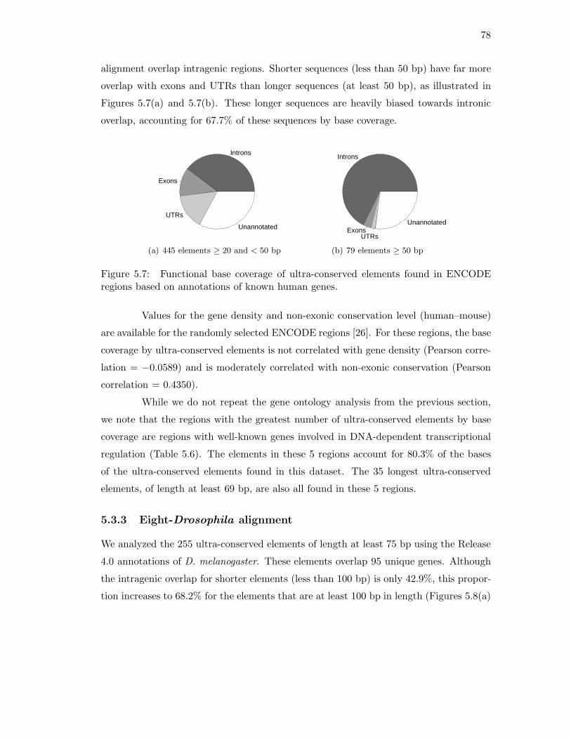
78
alignment overlap intragenic regions. Shorter sequences (less than 50 bp) have far more
overlap with exons and UTRs than longer sequences (at least 50 bp), as illustrated in
Figures 5.7(a) and 5.7(b). These longer sequences are heavily biased towards intronic
overlap, accounting for 67.7% of these sequences by base coverage.
Introns
Exons
UTRs
Unannotated
(a) 445 elements ≥ 20 and < 50 bp
Introns
ExonsUTRs
Unannotated
(b) 79 elements ≥ 50 bp
Figure 5.7: Functional base coverage of ultra-conserved elements found in ENCODEregions based on annotations of known human genes.
Values for the gene density and non-exonic conservation level (human–mouse)
are available for the randomly selected ENCODE regions [26]. For these regions, the base
coverage by ultra-conserved elements is not correlated with gene density (Pearson corre-
lation = −0.0589) and is moderately correlated with non-exonic conservation (Pearson
correlation = 0.4350).
While we do not repeat the gene ontology analysis from the previous section,
we note that the regions with the greatest number of ultra-conserved elements by base
coverage are regions with well-known genes involved in DNA-dependent transcriptional
regulation (Table 5.6). The elements in these 5 regions account for 80.3% of the bases
of the ultra-conserved elements found in this dataset. The 35 longest ultra-conserved
elements, of length at least 69 bp, are also all found in these 5 regions.
5.3.3 Eight-Drosophila alignment
We analyzed the 255 ultra-conserved elements of length at least 75 bp using the Release
4.0 annotations of D. melanogaster. These elements overlap 95 unique genes. Although
the intragenic overlap for shorter elements (less than 100 bp) is only 42.9%, this propor-
tion increases to 68.2% for the elements that are at least 100 bp in length (Figures 5.8(a)
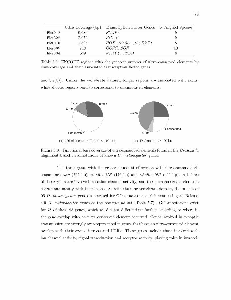
79
Ultra Coverage (bp) Transcription Factor Genes # Aligned Species
ENm012 9,086 FOXP2 9ENr322 2,072 BC11B 9ENm010 1,895 HOXA1-7,9-11,13 ; EVX1 8ENm005 718 GCFC ; SON 10ENr334 549 FOXP4 ; TFEB 8
Table 5.6: ENCODE regions with the greatest number of ultra-conserved elements bybase coverage and their associated transcription factor genes.
and 5.8(b)). Unlike the vertebrate dataset, longer regions are associated with exons,
while shorter regions tend to correspond to unannotated elements.
IntronsExons
UTRs
Unannotated
(a) 196 elements ≥ 75 and < 100 bp
Introns
Exons
UTRsUnannotated
(b) 59 elements ≥ 100 bp
Figure 5.8: Functional base coverage of ultra-conserved elements found in the Drosophilaalignment based on annotations of known D. melanogaster genes.
The three genes with the greatest amount of overlap with ultra-conserved el-
ements are para (765 bp), nAcRα-34E (426 bp) and nAcRα-30D (409 bp). All three
of these genes are involved in cation channel activity, and the ultra-conserved elements
correspond mostly with their exons. As with the nine-vertebrate dataset, the full set of
95 D. melanogaster genes is assessed for GO annotation enrichment, using all Release
4.0 D. melanogaster genes as the background set (Table 5.7). GO annotations exist
for 78 of these 95 genes, which we did not differentiate further according to where in
the gene overlap with an ultra-conserved element occurred. Genes involved in synaptic
transmission are strongly over-represented in genes that have an ultra-conserved element
overlap with their exons, introns and UTRs. These genes include those involved with
ion channel activity, signal transduction and receptor activity, playing roles in intracel-

80
lular signaling cascades, muscle contraction, development, and behavior. RNA binding
proteins are also found to be over-represented. Another group of over-represented genes
are those involved in RNA polymerase II transcription factor activity. These genes are
strongly associated with development and morphogenesis.
The 130 ultra-conserved elements found in unannotated regions are grouped
together into 109 regions by common flanking genes. These regions are flanked by 208
unique genes, 134 of which have available GO annotations. The distance from these
ultra-conserved elements to their respective nearest gene ranges from 0.2–104 kb and
is 16 kb on average. A number of transcription factors involved with development
and morphogenesis are found within this set of genes. Five of the 10 flanking genes
with ultra-conserved sequences both upstream and downstream are transcription factors
(SoxN, salr, toe, H15, sob). In total, 44 unique transcription factors are found across the
intragenic and flanking gene hits.
Ten of the original 255 ultra-conserved elements are repeated elsewhere in the
D. melanogaster genome. However, all of these repeats correspond to annotated tRNA or
snRNA, but not to homologous exons or regulatory regions. There are 10 ultra-conserved
elements that overlap with tRNA (757 bp in sum), two that overlap with snRNA (191
bp in sum), and one that overlaps with ncRNA (81 bp). None of the ultra-conserved
elements correspond to annotated rRNA, regulatory regions, transposable elements, or
pseudogenes.
5.3.4 Discussion
We studied ultra-conserved elements in three very different datasets: an alignment of
nine distant vertebrates, an alignment of the ENCODE regions in mammals, and an
alignment of eight fruit flies. As Figures 5.5, 5.7, and 5.8 show, ultra-conserved elements
overlap with genes very differently in the three datasets. In particular, in the Drosophila
dataset, exonic conservation is much more substantial. This conservation at the DNA
level is very surprising, as the functional constraint on coding regions is expected to
be at the amino acid level. Therefore, the degeneracy of the genetic code should allow
synonymous mutations to occur without any selective constraint.
The GO analysis showed that non-coding regions near or in genes associated
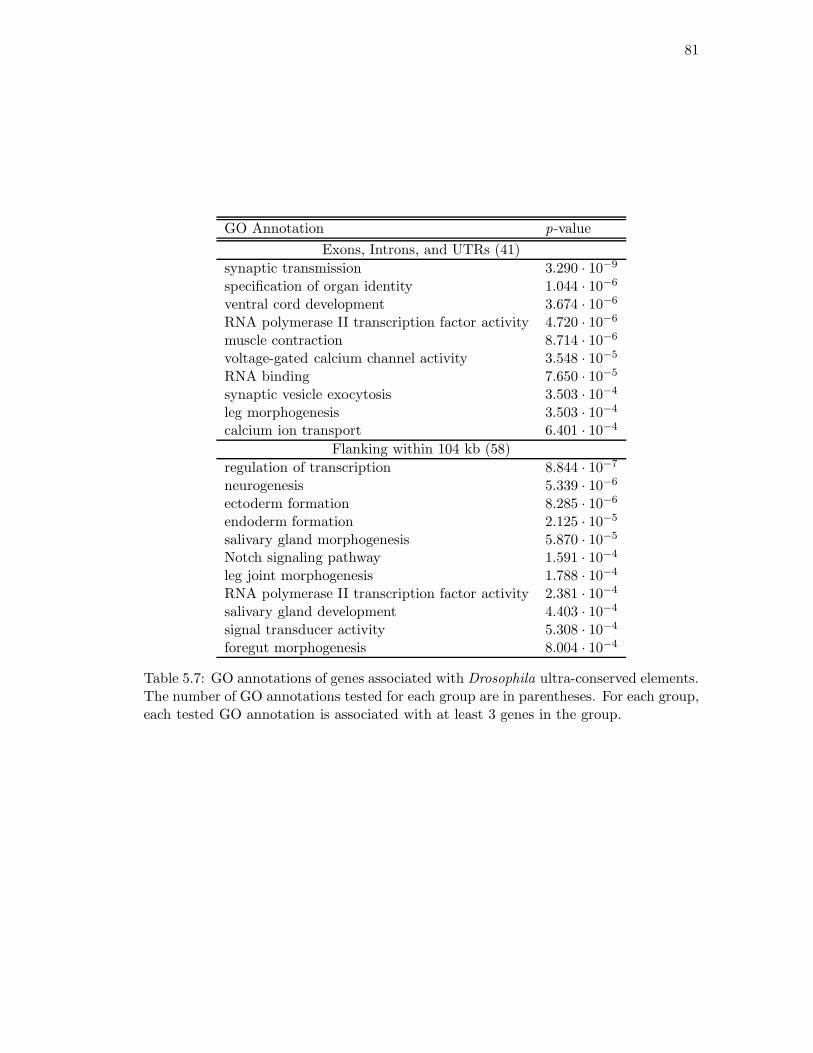
81
GO Annotation p-value
Exons, Introns, and UTRs (41)
synaptic transmission 3.290 · 10−9
specification of organ identity 1.044 · 10−6
ventral cord development 3.674 · 10−6
RNA polymerase II transcription factor activity 4.720 · 10−6
muscle contraction 8.714 · 10−6
voltage-gated calcium channel activity 3.548 · 10−5
RNA binding 7.650 · 10−5
synaptic vesicle exocytosis 3.503 · 10−4
leg morphogenesis 3.503 · 10−4
calcium ion transport 6.401 · 10−4
Flanking within 104 kb (58)
regulation of transcription 8.844 · 10−7
neurogenesis 5.339 · 10−6
ectoderm formation 8.285 · 10−6
endoderm formation 2.125 · 10−5
salivary gland morphogenesis 5.870 · 10−5
Notch signaling pathway 1.591 · 10−4
leg joint morphogenesis 1.788 · 10−4
RNA polymerase II transcription factor activity 2.381 · 10−4
salivary gland development 4.403 · 10−4
signal transducer activity 5.308 · 10−4
foregut morphogenesis 8.004 · 10−4
Table 5.7: GO annotations of genes associated with Drosophila ultra-conserved elements.The number of GO annotations tested for each group are in parentheses. For each group,each tested GO annotation is associated with at least 3 genes in the group.
82
with transcriptional regulation tended to contain ultra-conserved elements in all datasets.
In Drosophila, ultra-conserved elements overlapped primarily with genes associated with
synaptic transmission. While the exonic conservation in Drosophila is due in part to a
much shorter period of evolution, the exact conservation of exons whose gene products
are involved in synaptic transmission may be fly-specific.
Non-coding regions that are perfectly conserved across all 9 species may be
precise regulatory signals for highly specific DNA-binding proteins. In particular, re-
peated ultra-conserved elements such as those found near the Iroquois homeobox genes
on chromosome 16 are excellent candidates for such regulatory elements. Of course, it
is interesting to note that the degree of conservation in our ultra-conserved elements
exceeds what is observed for other known functional elements, such as splice sites. We
discuss the statistical significance of ultra-conservation in Section 5.4.
5.4 Statistical significance of ultra-conservation
Which ultra-conserved elements are of a length that is statistically significant? In order
to address this question, we choose a model and compute the probability of observing
an ultra-conserved element of a given length for the nine-vertebrate and Drosophila-
alignments. First we consider phylogenetic tree models. These models allow for depen-
dence of the occurrence of nucleotides in the genomes of different species at any given
position in the aligned genomes, but make the assumption that evolutionary changes to
DNA at one position in the alignment occur independently from changes at all other,
and in particular, neighboring positions. Later we also consider a Markov chain, which
does not model evolutionary changes explicitly but incorporates a simple pattern of
dependence among different genome positions.
Before being able to compute a probability in a phylogenetic tree model, we
must build a tree and estimate the parameters of the associated model. The tree for
the nine-vertebrate alignment is shown in Figure 5.1. The topology of this tree is well-
known, so we assume it fixed and use PAML [107] to estimate model parameters by
maximum likelihood. As input to PAML, we choose the entire alignments with all columns
containing a gap removed. The resulting alignment was 6,300,344 positions long for the
83
vertebrates and 26,216,615 positions long for the Drosophila. Other authors (e.g., [74])
have chosen to focus only on synonymous substitutions in coding regions, since they are
likely not selected for or against and thus give good estimates for neutral substitution
rates. However, our independence model does not depend on the functional structure
of the genome; that is, it sees the columns as i.i.d. samples. Thus, we believe that it is
more appropriate to use all the data available to estimate parameters.
There are many phylogenetic tree models (cf. Section 1.4) and we concentrate
here on the Jukes–Cantor and HKY85 models. With the parameter estimates from PAML,
we can compute the probability pcons of observing an ultra-conserved position in the
alignment. Recall that the probability pi1...is of seeing the nucleotide vector (i1, . . . , is) ∈
{A, C, G, T}s in a column of the alignment of s species is given by a polynomial in the
entries of the transition matrices Pe(t), which are obtained as Pe(t) = exp(Qte) where te
is the length of the edge e in the phylogenetic tree and Q is a rate matrix that depends
on the model selected.
Under the Jukes–Cantor model for the nine-vertebrate alignment, the maximum
likelihood (ML) branch lengths are shown in Figure 5.1 and give the probabilities
pAAAAAAAAA = · · · = pTTTTTTTTT = 0.01139...
Thus, the probability of a conserved column under this model is pcons = 0.0456. If we
require that the nucleotides are identical not only across present-day species but also
across ancestors, then the probability drops slightly to 0.0434.
Under the HKY85 model for the nine-vertebrate alignment, the ML branch
lengths are very similar to those in Figure 5.1 and the additional parameter is esti-
mated as κ = 2.4066. The root distribution is estimated to be almost uniform. These
parameters give the probabilities
pAAAAAAAAA = · · · = pTTTTTTTTT = 0.00367,
which are much smaller than their counterpart in the Jukes–Cantor model. The HKY85
probability of a conserved column is pcons = 0.014706. If we assume that nucleotides
must also be identical in ancestors, this probability drops to 0.01234.
The binary indicators of ultra-conservation are independent and identically
distributed according to a Bernoulli distribution with success probability pcons. The
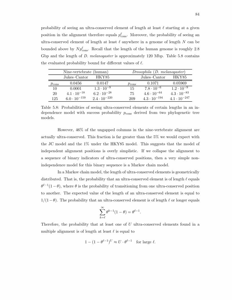
84
probability of seeing an ultra-conserved element of length at least ℓ starting at a given
position in the alignment therefore equals pℓcons. Moreover, the probability of seeing an
ultra-conserved element of length at least ℓ anywhere in a genome of length N can be
bounded above by Npℓcons. Recall that the length of the human genome is roughly 2.8
Gbp and the length of D. melanogaster is approximately 120 Mbp. Table 5.8 contains
the evaluated probability bound for different values of ℓ.
Nine-vertebrate (human) Drosophila (D. melanogaster)
Jukes–Cantor HKY85 Jukes–Cantor HKY85
pcons 0.0456 0.0147 pcons 0.1071 0.05969
10 0.0001 1.3 · 10−9 15 7.8 · 10−6 1.2 · 10−9
20 4.1 · 10−18 6.2 · 10−28 75 4.6 · 10−64 4.3 · 10−83
125 6.0 · 10−159 2.4 · 10−220 209 4.3 · 10−194 4.1 · 10−247
Table 5.8: Probabilities of seeing ultra-conserved elements of certain lengths in an in-dependence model with success probability pcons derived from two phylogenetic treemodels.
However, 46% of the ungapped columns in the nine-vertebrate alignment are
actually ultra-conserved. This fraction is far greater than the 5% we would expect with
the JC model and the 1% under the HKY85 model. This suggests that the model of
independent alignment positions is overly simplistic. If we collapse the alignment to
a sequence of binary indicators of ultra-conserved positions, then a very simple non-
independence model for this binary sequence is a Markov chain model.
In a Markov chain model, the length of ultra-conserved elements is geometrically
distributed. That is, the probability that an ultra-conserved element is of length ℓ equals
θℓ−1(1− θ), where θ is the probability of transitioning from one ultra-conserved position
to another. The expected value of the length of an ultra-conserved element is equal to
1/(1−θ). The probability that an ultra-conserved element is of length ℓ or longer equals
∞∑
k=ℓ
θk−1(1 − θ) = θℓ−1.
Therefore, the probability that at least one of U ultra-conserved elements found in a
multiple alignment is of length at least ℓ is equal to
1 − (1 − θℓ−1)U ≈ U · θℓ−1 for large ℓ.

85
Restricting ourselves to the nine-vertebrate alignment (computations for the
Drosophila alignment are qualitatively similar), we used the mean length of the ultra-
conserved elements described in Section 5.3.1 to estimate the transition probability θ to
0.4785. Then the probability that at least one of the 1,513,176 ultra-conserved elements
of the nine-vertebrate alignment is of length 25 or longer equals about 3%. The probabil-
ity of seeing one of the U ultra-conserved elements being 30 or more bp long is just below
1/1000. However, the dependence structure in a Markov chain model cannot explain the
longest ultra-conserved elements in the alignment. For example, the probability of one
of the U elements being 125 or more bp long is astronomically small (0.3× 10⁻³³). This
suggests that the Markov chain model does not capture the dependence structure in the
binary sequence of ultra-conservation indicators. At a visual level, this is clear from
Figure 5.3. Were the Markov chain model true then, due to the resulting geometric dis-
tribution for the length of an ultra-conserved element, the log-scale frequencies should
fall on a straight line, which is not the case in Figure 5.3. Modeling the process of ultra-
conservation statistically requires more sophisticated models. The phylogenetic hidden
Markov models that appear in [64, 87] provide a point of departure.
Despite the shortcomings of the calculations, it is clear that it is highly unlikely
that the ultra-conserved elements studied in this chapter occur by chance. The degree
of conservation strongly suggests extreme natural selection in these regions.
86
Chapter 6
Evolution on distributive lattices
In this chapter, we model the evolution of a population under strong selective
pressure using a probabilistic model on a distributive lattice. We describe how the
combinatorial structure of a distributive lattice arises naturally from both biology and
algebraic statistics. The probability that the population develops an escape mutant
before extinction is encoded in the algebraic combinatorics of the lattice.
Using methods from combinatorics and algebra, we analyze the problem of drug
resistance in HIV under treatment with the protease inhibitors ritonavir and indinavir.
We begin by explaining the problem of drug resistance in HIV in Section 6.1 and our
mathematical formulation is Section 6.2. The material in this chapter comes from the
paper [10] with Niko Beerenwinkel and Bernd Sturmfels.
The evolutionary fate of a population is determined by the replication dynamics
of the ensemble and by the reproductive success of its individuals. We are interested
in scenarios where most individuals have a low fitness, eventually leading to extinction,
and only a few types of individuals (“escape mutants”) can survive permanently. These
situations often arise due to a significant change of the underlying fitness landscape.
For example, a virus that has been transmitted to a new host is confronted with a new
immune response. Likewise, medical interventions such as radiation therapy, vaccination,
or chemotherapy result in altered fitness landscapes for the targeted agents, which may
be bacteria, viruses, or cancer cells.
Given a population and such a hostile fitness landscape, the central question is
87
whether the population will survive. In the case of medical interventions we wish to know
the probability of successful treatment. Answering this question involves computing the
risk of evolutionary escape, i.e., the probability that the population develops an escape
mutant before extinction. In this chapter, we present a mathematical framework for
computing such probabilities.
6.1 Drug resistance in HIV
Our primary application is the evolution of drug resistance during treatment of HIV
infected patients [23]. Drug resistance is the consequence of mutations in the viral
proteins which are targeted by antiretroviral drugs.
HIV is a retrovirus, which means that it uses RNA instead of DNA as its
genetic material. Its genome is about 10000 nucleotides in length with nine open reading
frames. Three of the precursor proteins that are produced, however, are cleaved by the
viral protease enzyme, giving a total of 15 proteins which are produced by HIV.
The HIV virus binds to the CD4 receptor of a host cell with the aid of further
cellular coreceptors and enters the cell. It then releases its genetic material (which is
carried in the form of RNA). This RNA is transcribed into DNA using the HIV enzyme
reverse transcriptase and enters the nucleus. There it is transcribed into mRNA and
translated into proteins using the machinery of the host cell. This allows for many
copies of the virus to be made in the host cell. These proteins have to be processed by
the HIV protease enzyme into their functional form before the new copy of the virus
can infect other cells. Different classes of drugs have been designed to attack the virus
during every step of the above process with impressive success. There are currently 27
drugs approved by the FDA in four different classes. These drugs are typically taken in
combinations of two to four drugs simultaneously from two different classes.
However, the reverse transcription step is notoriously error prone, producing
on average one error in every replication of the genome. This high mutation rate can
lead to the development of drug resistance. As many as 50 percent of patients receiving
antiretroviral therapy are infected with viruses which are resistant to one of the available
drugs [23]. Given this, it is key for doctors to have methods of determining the best
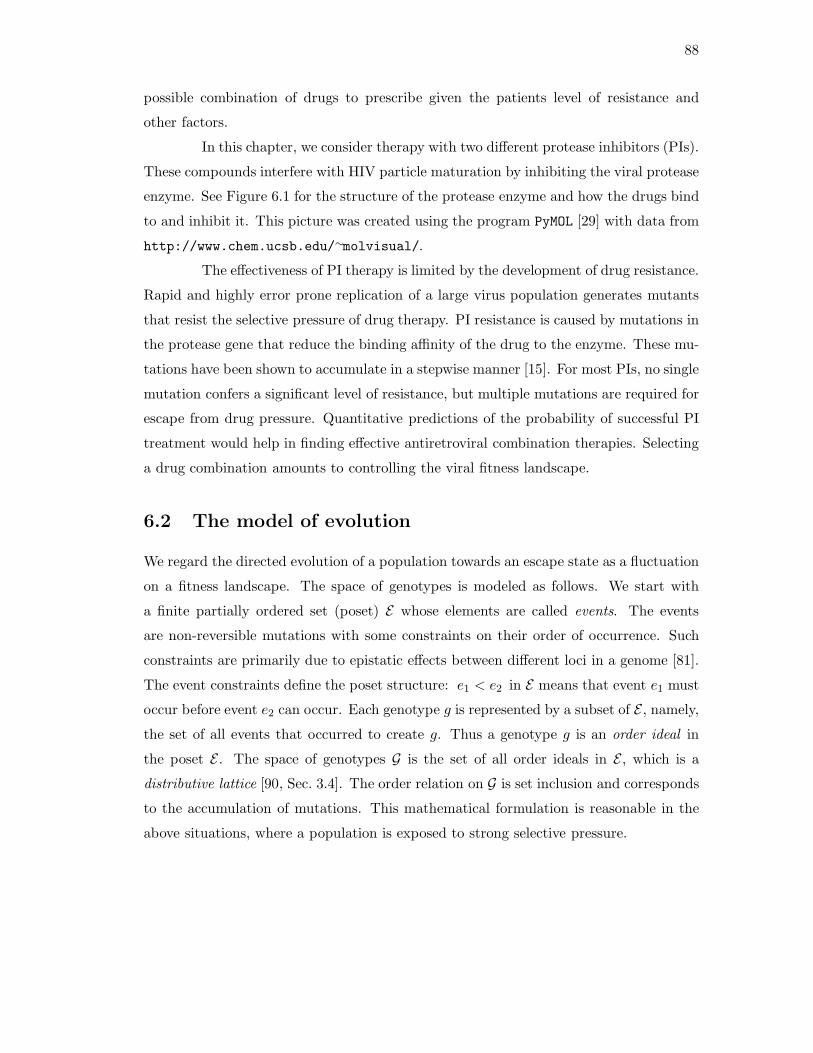
88
possible combination of drugs to prescribe given the patients level of resistance and
other factors.
In this chapter, we consider therapy with two different protease inhibitors (PIs).
These compounds interfere with HIV particle maturation by inhibiting the viral protease
enzyme. See Figure 6.1 for the structure of the protease enzyme and how the drugs bind
to and inhibit it. This picture was created using the program PyMOL [29] with data from
http://www.chem.ucsb.edu/∼molvisual/.
The effectiveness of PI therapy is limited by the development of drug resistance.
Rapid and highly error prone replication of a large virus population generates mutants
that resist the selective pressure of drug therapy. PI resistance is caused by mutations in
the protease gene that reduce the binding affinity of the drug to the enzyme. These mu-
tations have been shown to accumulate in a stepwise manner [15]. For most PIs, no single
mutation confers a significant level of resistance, but multiple mutations are required for
escape from drug pressure. Quantitative predictions of the probability of successful PI
treatment would help in finding effective antiretroviral combination therapies. Selecting
a drug combination amounts to controlling the viral fitness landscape.
6.2 The model of evolution
We regard the directed evolution of a population towards an escape state as a fluctuation
on a fitness landscape. The space of genotypes is modeled as follows. We start with
a finite partially ordered set (poset) E whose elements are called events. The events
are non-reversible mutations with some constraints on their order of occurrence. Such
constraints are primarily due to epistatic effects between different loci in a genome [81].
The event constraints define the poset structure: e1 < e2 in E means that event e1 must
occur before event e2 can occur. Each genotype g is represented by a subset of E , namely,
the set of all events that occurred to create g. Thus a genotype g is an order ideal in
the poset E . The space of genotypes G is the set of all order ideals in E , which is a
distributive lattice [90, Sec. 3.4]. The order relation on G is set inclusion and corresponds
to the accumulation of mutations. This mathematical formulation is reasonable in the
above situations, where a population is exposed to strong selective pressure.
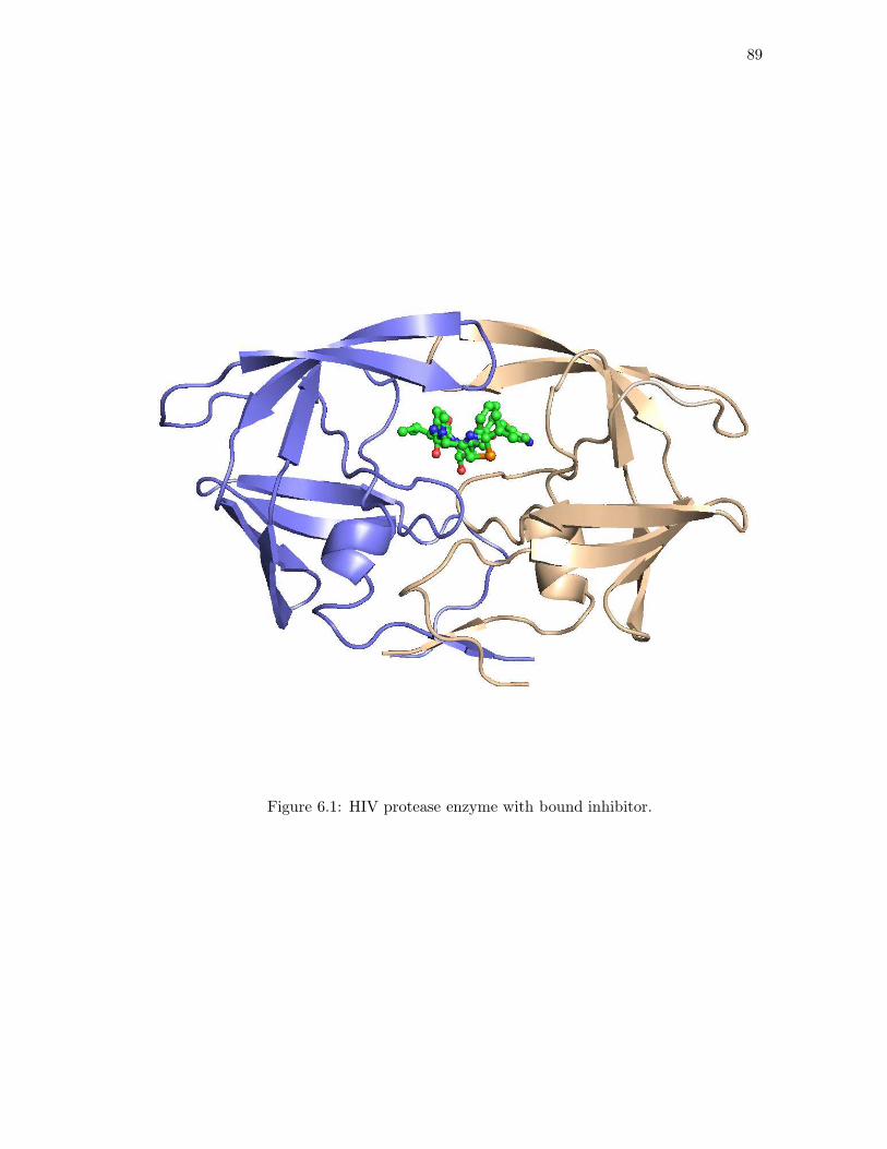
89
Figure 6.1: HIV protease enzyme with bound inhibitor.
90
0100
0000
1111
0101
1110
1100
1101
10001 2
43
Figure 6.2: An event poset, its genotype lattice, and a fitness landscape.
The risk of escape is governed by the structure of G, the fitness function on
G, and the population dynamics (such as the mutation rates and population size). Our
focus is on the dependency of the risk of escape on the assigned fitness values for each
genotype g ∈ G. This leads us to the risk polynomial, which is shown to be equivalent
to a well-known object in algebraic combinatorics. Indeed, one of the objectives of this
work is to provide a bridge between algebraic combinatorics and evolutionary biology.
This chapter is organized as follows. In Section 6.3 we formalize our model of
a static fitness landscape on the genotype lattice G derived from an event poset E , and
we discuss evolution on the lattice G. In Section 6.4 we review the multistate branching
process studied by Iwasa, Michor and Nowak [54, 55].
In Section 6.5 we study the Bayesian networks which arise from identifying the
events in E with binary random variables. These statistical models can be used to infer
the genotype space from given data. For conjunctive Bayesian networks we recover the
distributive lattice of order ideals in E . Of particular interest is the case where E is
a directed forest: here the Bayesian network is a mutagenetic tree model [9, 12]. The
application of our methods to the development of PI resistance in HIV is presented in
Section 6.6.
Section 6.7 summarizes various representations of the risk polynomial in terms
of structures from algebraic combinatorics. Efficient methods for computing the risk
polynomial and their implementation are presented.

91
6.3 Fitness landscapes on distributive lattices
A partially ordered set (or poset) is a set E together with a binary relation, denoted
“≤”, which is reflexive, antisymmetric, and transitive. Here we fix a finite poset E whose
elements are called events. If the number of events is n then we often identify the set
underlying E with the set [n] = {1, 2, . . . , n}. In this way, the subsets of E are encoded
by the 2n binary strings of length n. The empty subset of E is encoded by the all-zero
string 0 = 00 · · · 0 which represents the wild type, and the full set E is encoded by the
all-one string 1 = 11 · · · 1 which represents the escape state.
An order ideal g in a poset E is a subset of E that is closed downward; that is,
if e2 ∈ g and e1 ≤ e2, then e1 ∈ g. The set of all order ideals of E forms a distributive
lattice J(E) under inclusion. Birkhoff’s Representation Theorem [90, Thm. 3.4.1] states
that all distributive lattices have the form J(E) for a poset E . We write G = J(E), and
we call G the genotype lattice.
Example 6.1. Let E be the trivial poset, where no two events are comparable, with
|E| = n. Then G = J(E) is the Boolean lattice consisting of all subsets of E ordered by
inclusion. This means that all possible combinations of mutations are possible, and they
can occur in any order. Each of the 2n binary strings g ∈ {0, 1}n represents a mutational
pattern, or genotype.
In general, the event poset E does have non-trivial relations e1 < e2. The
relation e1 < e2 excludes all genotypes g with ge1 = 0 and ge2 = 1 from G. The remaining
genotypes g form a sublattice of the Boolean lattice {0, 1}n, and this is precisely our
distributive lattice G = J(E). Note that the lattice G is ranked, with the rank function
given by rank(g) = |g|.
Example 6.2. Consider a scenario with n = 4 mutation events, labeled E = {1, 2, 3, 4}.
Suppose that event 3 can only occur after events 1 and 2, and event 4 can only occur
after event 2. This allows for precisely eight genotypes
G ={
0000, 1000, 0100, 1100, 0101, 1110, 1101, 1111}
.
The event poset E and the genotype lattice G are shown in Figure 6.2.

92
A fitness landscape associates to each possible genotype a number which quan-
tifies the reproductive capacity of an individual with that genotype [79]. We define a
fitness landscape on the distributive lattice G to be any function f : G → R. The value
f(g) at any g ∈ G is the fitness of the genotype g. Thus, the space of all fitness landscapes
is the finite-dimensional vector space RG.
We shall consider certain special models of fitness landscapes, which are repre-
sented by linear subspaces of RG . In the following definitions, a genotype g is regarded
as a subset of the event poset E , where |E| = n. A constant fitness landscape has the
form f(g) ≡ a for some constant a. Thus the constant landscapes form a line through
the origin in RG . A graded fitness landscape is a landscape on G whose fitness values
depend only on the rank. Equivalently, we have f(g) = a|g| for constants a0, a1, . . . , an.
Thus, graded fitness landscapes form an (n + 1)-dimensional linear subspace of RG.
Our biological application in Section 6.6 uses the graded fitness landscape
model, which means that the fitness of a virus type depends only on the number of
mutations it harbors. We shall model situations where a virus escapes from a wild type
0 to a drug-resistant type 1. In this case, we assume a graded fitness landscape that is
monotonically increasing with rank, i.e.,
a0 < a1 < a2 < · · · < an.
This implies that the fitness landscape f has a unique local (and global) maximum at
the drug resistant type 1, which is the top element in G.
We next introduce the mathematical framework for evolution on a fitness land-
scape. The general setup is as in the work of Reidys and Stadler [79], but this is adapted
here to our specific situation, where the genotypes form a distributive lattice G. The
order relation on G, which comes from inclusion of subsets of E , induces a neighborhood
structure on G where the neighbors of g ∈ G are the genotypes that strictly contain g,
N(g) :={
h ∈ G | g ⊂ h}
. (6.1)
Unlike the typical situation considered in [79], this notion of neighborhood is not sym-
metric. To be precise, we have that h ∈ N(g) implies g 6∈ N(h).
This neighborhood structure implies that mutational changes are possible only
upward in the genotype lattice. This structure models a directed evolutionary process
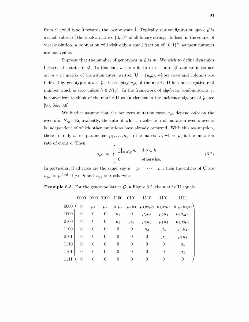
93
from the wild type 0 towards the escape state 1. Typically, our configuration space G is
a small subset of the Boolean lattice {0, 1}n of all binary strings. Indeed, in the course of
viral evolution, a population will visit only a small fraction of {0, 1}n, as most mutants
are not viable.
Suppose that the number of genotypes in G is m. We wish to define dynamics
between the states of G. To this end, we fix a linear extension of G, and we introduce
an m × m matrix of transition rates, written U = (ugh), whose rows and columns are
indexed by genotypes g, h ∈ G. Each entry ugh of the matrix U is a non-negative real
number which is zero unless h ∈ N(g). In the framework of algebraic combinatorics, it
is convenient to think of the matrix U as an element in the incidence algebra of G; see
[90, Sec. 3.6].
We further assume that the non-zero mutation rates ugh depend only on the
events in h\g. Equivalently, the rate at which a collection of mutation events occurs
is independent of which other mutations have already occurred. With this assumption,
there are only n free parameters µ1, . . . , µn in the matrix U, where µe is the mutation
rate of event e. Then
ugh =
∏
e∈h\g µe if g ⊂ h
0 otherwise.(6.2)
In particular, if all rates are the same, say µ = µ1 = · · · = µn, then the entries of U are
ugh = µ|h\g| if g ⊂ h and ugh = 0 otherwise.
Example 6.3. For the genotype lattice G in Figure 6.2, the matrix U equals
0000 1000 0100 1100 0101 1110 1101 1111
0000 0 µ1 µ2 µ1µ2 µ2µ4 µ1µ2µ3 µ1µ2µ4 µ1µ2µ3µ4
1000 0 0 0 µ2 0 µ2µ3 µ2µ4 µ2µ3µ4
0100 0 0 0 µ1 µ4 µ1µ3 µ1µ4 µ1µ3µ4
1100 0 0 0 0 0 µ3 µ4 µ3µ4
0101 0 0 0 0 0 0 µ1 µ1µ3
1110 0 0 0 0 0 0 0 µ4
1101 0 0 0 0 0 0 0 µ3
1111 0 0 0 0 0 0 0 0

94
Note that the entry in row g and column h of any power Uk equals ugh times the number
of paths of length k from g to h in G. In particular, U5 = 0.
Let f be a fitness landscape on G and F = diag(
f(g) | g ∈ G)
the m × m
diagonal matrix whose entries are the fitness values. The entry of the matrix product
UF in row g and column h represents the probability of genotype g transitioning into
genotype h in one step. A precise probabilistic derivation and interpretation will be
given in the next section.
We are interested in all mutational pathways that lead from the wild type 0
to the escape state 1. Towards this end, note that the entry (g, h) of the matrix (UF)k
represents the probability of genotype g evolving to genotype h along any mutational
pathway (chain) of length k in the genotype lattice G. The chains from 0 to 1 in G are
accounted for by the upper right hand entry of (UF)k. Note that the matrix (UF)k is
zero for k > n.
To account for chains of arbitrary length, we consider the matrix
(I − UF)−1 − I = UF + (UF)2 + (UF)3 + · · · + (UF)n, (6.3)
where I is the m × m identity matrix. We summarize our discussion in the following
proposition, which is proved by elementary matrix algebra.
Proposition 6.4. The entry of the matrix (6.3) in row g and column h is zero unless
g ⊂ h, in which case it is ugh · f(h) ·Pgh(f) where Pgh is a polynomial function of degree
|h\g| − 1 on the space of all fitness landscapes RG.
The polynomial Pgh(f) is the generating function for all chains from g to h in
G. This will be made precise in the following corollary. We shall restrict ourselves to the
most important case when g = 0 is the wild type and h = 1 is the escape state. Studying
P01(f) only is no loss of generality because any interval of a distributive lattice is again
a distributive lattice.
Proposition 6.4 tells us that P01(f) is a polynomial of degree n − 1 in the
unknown fitness values f(g), which are also written as fg, where g ∈ G.

95
Corollary 6.5. The polynomial P01(f) in the upper-right entry of (6.3) equals
P01(f) =∑
0=g0⊂g1⊂···⊂gk=1
fg1fg2 · · · fgk−1, (6.4)
where the sum runs over all chains from 0 to 1 in the genotype lattice G.
6.4 The risk of escape
For a poset of events E and the corresponding distributive lattice G = J(E), the risk
polynomial of G is defined as the polynomial (6.4), which we denote by R(G; f). The
risk polynomial was introduced in [54, 55]. In this section we review the evolutionary
dynamics model proposed in these papers, and we discuss the probabilistic meaning of
the risk polynomial.
Example 6.6. Let G be the genotype lattice in Figure 6.2. Then the risk polynomial
R(G; f) is the following polynomial of degree three in six unknowns:
1 + f1000 + f0100 + f1100 + f0101 + f1110 + f1101
+f1000f1100 + f0100f1100 + f0100f0101 + f1000f1110 + f0100f1110
+f1000f1101 + f0100f1101 + f1100f1110 + f1100f1101 + f0101f1101
+f1000f1100f1110 + f0100f1100f1110 + f1000f1100f1101
+f0100f1100f1101 + f0100f0101f1101.
If we restrict the fitness landscape f to lie in a linear subspace of RG , then
R(G; f) specializes to a polynomial in fewer unknowns. For example, the risk polynomial
for graded fitness landscapes is obtained from the specialization f(g) = a|g|. That risk
polynomial has degree n−1 and is denoted by R(G; a1, . . . , an−1). For instance, R(G; f)
in Example 6.6 specializes to
R(G; a1, a2, a3) = 1 + 2a1 + 2a2 + 2a3 + 3a1a2 + 4a1a3 + 3a2a3 + 5a1a2a3.
For constant fitness landscapes f ≡ a , the risk polynomial is a polynomial in one un-
known a. It is denoted R(G; a). In our running example,
R(G; a) = 1 + 6a + 10a2 + 5a3.
96
We now make precise the notion of risk of escape, which will justify our def-
inition of the risk polynomial. Our derivation is based on the model for the dynamics
of a replicating population on a fitness landscape studied by Iwasa, Michor and Nowak
[54, 55]. See also the work of Wilke [105] and the references given therein for approaches
to computing fixation probabilities.
A multistate branching process [6] consists of a set of genotypes along with a
fitness landscape and mutation rates between genotypes. We assume a discrete time
process, where in one generation an individual with genotype g has a random number of
offspring following a Poisson distribution with mean Rg. Some of these offspring may be
mutants according to the mutation rates ugh. The parameter Rg is the basic reproductive
ratio [69, Chap. 3].
We assume there is no interaction between individuals; each reproduces at a
rate independent of the distribution of the population. Let ρkg,h be the probability that
one individual of genotype g has k children of type h. Then,
ρkg,h =
(ughRg)k · e−ughRg
k!. (6.5)
The reproductive fitness fg is related to the reproductive ratio Rg by
fg =Rg
1 − Rgand Rg =
fg
1 + fg. (6.6)
Let ξg be the probability of escape starting with one individual of genotype g,
so 1 − ξg is the probability of extinction. In particular, ξ1 is the probability that one
resistant virus will not become extinct. Each of these probabilities is a function of the
mutation rates ugh and the reproductive ratios Rg. We assume that the ugh are as in
(6.2), but with ugg = 1. Thus, each escape probability ξg can be expressed as a function
of the µe for e ∈ E and (using the relation (6.6)) the fitness values fg for g ∈ G.
Theorem 6.7. If ξg ≪ 1 for g 6= 1, then the probability of escape on the fitness landscape
f ∈ RG starting with one individual of wild type 0, satisfies
ξ0 ≈ ξ1 · f0 ·∏
e∈E
µe · R(G; f). (6.7)

97
Proof. The probability of extinction satisfies the recursive formula
1 − ξg =∏
h⊇g
∞∑
k=0
(1 − ξh)k · ρkg,h. (6.8)
Using (6.5), the right hand side of (6.8) can be rewritten as follows:
∏
h⊇g
exp((1 − ξh)ughRg) · exp(−ughRg) = exp
∑
h⊇g
−ξhughRg
.
We conclude that
log(1 − ξg) = −∑
h⊇g
ξhughRg for all g ∈ G.
Under the assumption that ξg ≪ 1 for g 6= 1, we can linearize the logarithms using the
relation log(1 − ξg) ≈ −ξg. This implies, for g ∈ G\{1},
ξg ≈ Rg ·∑
h⊇g ξhugh
=Rg
1−Rgugg·∑
h⊃g ξhugh
= fg ·∑
h⊃g ξhugh.
The theorem now follows by setting g = 0 and expanding the last equation
recursively. Here we are using the fact from (6.2) that the product of the ugh over any
chain from 0 to 1 in G equals∏
e∈E µe.
The typical situation of interest is a fitness landscape for which only the escape
state has a basic reproductive ratio greater than one, i.e.,
R1 > 1 and Rg < 1 for all g 6= 1.
When the positive numbers Rg are very small for g ∈ G\{1} then the approximation
(6.7) is valid, and it shows the crucial role that the risk polynomial R(G; f) plays in
assessing the risk of escape from the wild type 0 to the escape state 1. The theorem
implies that the risk of escape of a population of N wild type viruses is (1 − ξ0)N . In
Section 6.8 we discuss the situation in which the population is not homogeneous at the
time of intervention.
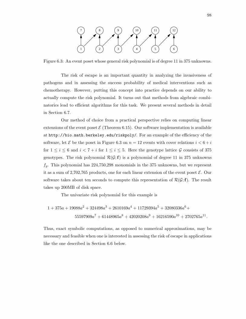
98
52 3 4 6
12111098
1
7
Figure 6.3: An event poset whose general risk polynomial is of degree 11 in 375 unknowns.
The risk of escape is an important quantity in analyzing the invasiveness of
pathogens and in assessing the success probability of medical interventions such as
chemotherapy. However, putting this concept into practice depends on our ability to
actually compute the risk polynomial. It turns out that methods from algebraic combi-
natorics lead to efficient algorithms for this task. We present several methods in detail
in Section 6.7.
Our method of choice from a practical perspective relies on computing linear
extensions of the event poset E (Theorem 6.15). Our software implementation is available
at http://bio.math.berkeley.edu/riskpoly/. For an example of the efficiency of the
software, let E be the poset in Figure 6.3 on n = 12 events with cover relations i < 6 + i
for 1 ≤ i ≤ 6 and i < 7 + i for 1 ≤ i ≤ 5. Here the genotype lattice G consists of 375
genotypes. The risk polynomial R(G; f) is a polynomial of degree 11 in 375 unknowns
fg. This polynomial has 224,750,298 monomials in the 375 unknowns, but we represent
it as a sum of 2,702,765 products, one for each linear extension of the event poset E . Our
software takes about ten seconds to compute this representation of R(G; f). The result
takes up 200MB of disk space.
The univariate risk polynomial for this example is
1 + 375a + 19088a2 + 324498a3 + 2610169a4 + 11729394a5 + 32080336a6+
55597909a7 + 61448965a8 + 42020208a9 + 16216590a10 + 2702765a11 .
Thus, exact symbolic computations, as opposed to numerical approximations, may be
necessary and feasible when one is interested in assessing the risk of escape in applications
like the one described in Section 6.6 below.
99
6.5 Distributive lattices from Bayesian networks
In this section, we present a family of statistical models that naturally gives rise to
distributive lattices. This statistical interpretation provides a method for deriving the
genotype lattice G directly from data. The basic idea is to estimate the poset structure
on E from observed genotypes, by applying model selection techniques to a range of
Bayesian networks, and to define G as the set of all genotypes with non-zero probability
in the model.
We first make precise the derivation of a genotype space from a statistical
model. Let E be an unordered set of n genetic events. The events are labeled by
1, 2, . . . , n. Subsets of E are identified with binary strings g ∈ {0, 1}n. They are the
possible genotypes. We consider binary random variables XE = (X1, . . . ,Xn), where
Xe = 1 indicates the occurrence of event e. Let ∆ denote the (2n − 1)-dimensional
simplex of probability distributions on {0, 1}n. A statistical model for XE is a map
p : Θ → ∆, where Θ is some parameter space. The g-th coordinate of p, denoted pg, is
the probability of genotype g ∈ {0, 1}n under the model p. The induced genotype space
of the model p : Θ → ∆ is the set Gp of all strings g ∈ {0, 1}n such that pg is not the
zero function on Θ. We regard Gp as a poset ordered by inclusion.
Now consider a directed acyclic graph on the set of events E . We will also call
this graph E . The Bayesian network model, or directed acyclic graphical model, defined
by E is the family of joint distributions that factor as
Pr(X1, . . . ,Xn) =∏
e∈E
Pr(Xe | Xpa(e)),
where pa(e) denotes the set of parents of e in E . Equivalently, a Bayesian network is
specified by a set of conditional independence statements. Each node is independent of
its ancestors given its parents. See [61] for an introduction to the relevant statistical
theory and [51] for an algebraic perspective.
The parameters for a Bayesian network are specified by providing, for each
event e ∈ E , a 2|pa(e)| × 2 matrix θe. The matrix entries are
θegpa(e),ge
= Pr(
Xe = ge | Xpa(e) = gpa(e)
)
,

100
for gpa(e) ∈ {0, 1}pa(e), ge ∈ {0, 1}. These conditional probabilities satisfy
θegpa(e),0
≥ 0 , θegpa(e),1
≥ 0 and θegpa(e),0
+ θegpa(e),1
= 1. (6.9)
Set d =∑
e∈E 2|pa(e)| and Θ = [0, 1]d. The points in the cube Θ are identified
with n-tuples of matrices θ = (θe | e ∈ E) as above. The general Bayesian network is
the polynomial map p : Θ → ∆ whose coordinates are
pg(θ) =∏
e∈E
θegpa(e),ge
. (6.10)
The general Bayesian network on E induces the genotype space Gp = {0, 1}n, the Boolean
lattice on E . Indeed, the factorization (6.10) implies that no genotype g ∈ {0, 1}n has
probability zero for all parameter values.
To obtain other genotype spaces, we replace the cube Θ = [0, 1]d by one of its
faces, as follows. For each event e ∈ E consider a Boolean function βe : {0, 1}pa(e) →
{0, 1}. If βe(ge) = 0 then the row of the 2|pa(e)| × 2-matrix θe indexed by the genotype g
is fixed to be the vector (1, 0); otherwise that row remains indeterminate subject to the
constraints (6.9). Let Θβ denote the face of Θ determined by these requirements and
pβ : Θβ → ∆ the restriction of the polynomial map p to Θβ. The resulting model is the
Bayesian network on E constrained by the Boolean functions βe.
If all Boolean functions βe are disjunctions then we get the disjunctive Bayesian
network on E . In this model, an event e can only occur if at least one of its parent events
has already occurred. If all Boolean functions βe are conjunctions then we get the
conjunctive Bayesian network on E . In this model, an event e can only occur if all of its
parent events have already occurred. These restricted Bayesian network models induce
interesting genotype spaces. Our main result in this section concerns the conjunctive
case.
We regard the given directed acyclic graph E as a poset by setting e1 ≤ e2
if there exists a path from e1 to e2. We write pconj : [0, 1]n → ∆ for the conjunctive
Bayesian network on E , since it has precisely n free parameters.
Theorem 6.8. The genotype space induced by the conjunctive Bayesian network on E
is the distributive lattice of order ideals in E, i.e., Gpconj = J(E).
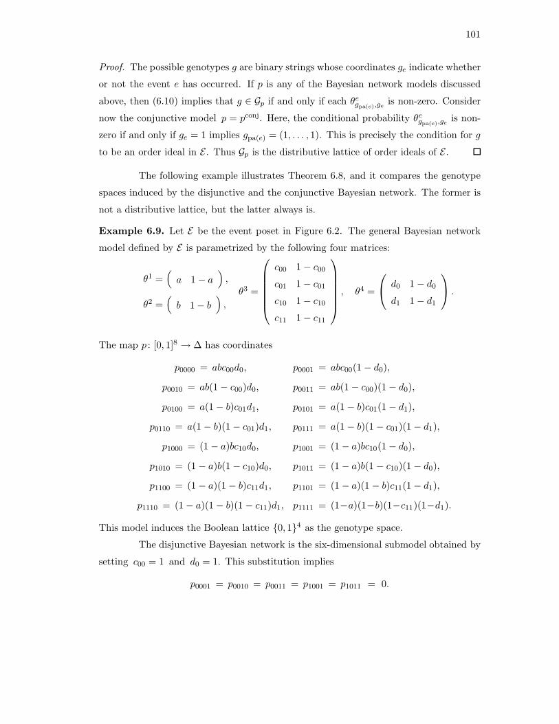
101
Proof. The possible genotypes g are binary strings whose coordinates ge indicate whether
or not the event e has occurred. If p is any of the Bayesian network models discussed
above, then (6.10) implies that g ∈ Gp if and only if each θegpa(e),ge
is non-zero. Consider
now the conjunctive model p = pconj. Here, the conditional probability θegpa(e),ge
is non-
zero if and only if ge = 1 implies gpa(e) = (1, . . . , 1). This is precisely the condition for g
to be an order ideal in E . Thus Gp is the distributive lattice of order ideals of E .
The following example illustrates Theorem 6.8, and it compares the genotype
spaces induced by the disjunctive and the conjunctive Bayesian network. The former is
not a distributive lattice, but the latter always is.
Example 6.9. Let E be the event poset in Figure 6.2. The general Bayesian network
model defined by E is parametrized by the following four matrices:
θ1 =(
a 1 − a)
,
θ2 =(
b 1 − b)
,
θ3 =
c00 1 − c00
c01 1 − c01
c10 1 − c10
c11 1 − c11
, θ4 =
d0 1 − d0
d1 1 − d1
.
The map p : [0, 1]8 → ∆ has coordinates
p0000 = abc00d0, p0001 = abc00(1 − d0),
p0010 = ab(1 − c00)d0, p0011 = ab(1 − c00)(1 − d0),
p0100 = a(1 − b)c01d1, p0101 = a(1 − b)c01(1 − d1),
p0110 = a(1 − b)(1 − c01)d1, p0111 = a(1 − b)(1 − c01)(1 − d1),
p1000 = (1 − a)bc10d0, p1001 = (1 − a)bc10(1 − d0),
p1010 = (1 − a)b(1 − c10)d0, p1011 = (1 − a)b(1 − c10)(1 − d0),
p1100 = (1 − a)(1 − b)c11d1, p1101 = (1 − a)(1 − b)c11(1 − d1),
p1110 = (1 − a)(1 − b)(1 − c11)d1, p1111 = (1−a)(1−b)(1−c11)(1−d1).
This model induces the Boolean lattice {0, 1}4 as the genotype space.
The disjunctive Bayesian network is the six-dimensional submodel obtained by
setting c00 = 1 and d0 = 1. This substitution implies
p0001 = p0010 = p0011 = p1001 = p1011 = 0.
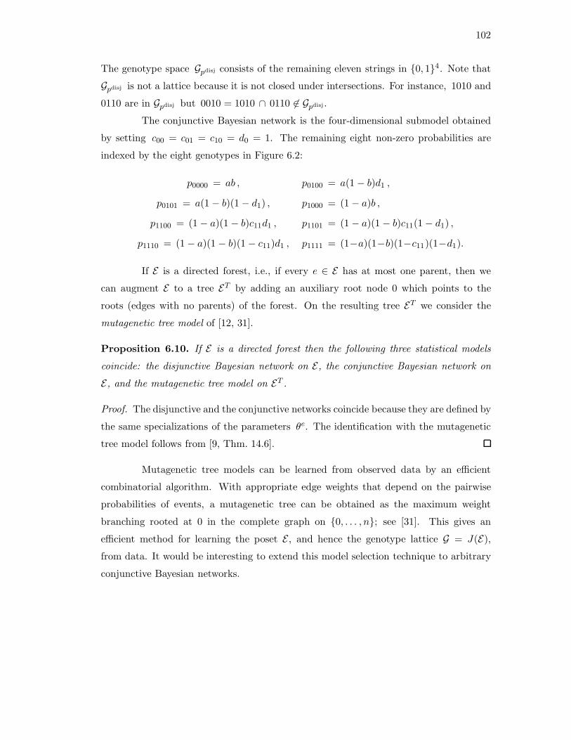
102
The genotype space Gpdisj consists of the remaining eleven strings in {0, 1}4. Note that
Gpdisj is not a lattice because it is not closed under intersections. For instance, 1010 and
0110 are in Gpdisj but 0010 = 1010 ∩ 0110 6∈ Gpdisj.
The conjunctive Bayesian network is the four-dimensional submodel obtained
by setting c00 = c01 = c10 = d0 = 1. The remaining eight non-zero probabilities are
indexed by the eight genotypes in Figure 6.2:
p0000 = ab , p0100 = a(1 − b)d1 ,
p0101 = a(1 − b)(1 − d1) , p1000 = (1 − a)b ,
p1100 = (1 − a)(1 − b)c11d1 , p1101 = (1 − a)(1 − b)c11(1 − d1) ,
p1110 = (1 − a)(1 − b)(1 − c11)d1 , p1111 = (1−a)(1−b)(1−c11)(1−d1).
If E is a directed forest, i.e., if every e ∈ E has at most one parent, then we
can augment E to a tree ET by adding an auxiliary root node 0 which points to the
roots (edges with no parents) of the forest. On the resulting tree ET we consider the
mutagenetic tree model of [12, 31].
Proposition 6.10. If E is a directed forest then the following three statistical models
coincide: the disjunctive Bayesian network on E, the conjunctive Bayesian network on
E, and the mutagenetic tree model on ET .
Proof. The disjunctive and the conjunctive networks coincide because they are defined by
the same specializations of the parameters θe. The identification with the mutagenetic
tree model follows from [9, Thm. 14.6].
Mutagenetic tree models can be learned from observed data by an efficient
combinatorial algorithm. With appropriate edge weights that depend on the pairwise
probabilities of events, a mutagenetic tree can be obtained as the maximum weight
branching rooted at 0 in the complete graph on {0, . . . , n}; see [31]. This gives an
efficient method for learning the poset E , and hence the genotype lattice G = J(E),
from data. It would be interesting to extend this model selection technique to arbitrary
conjunctive Bayesian networks.
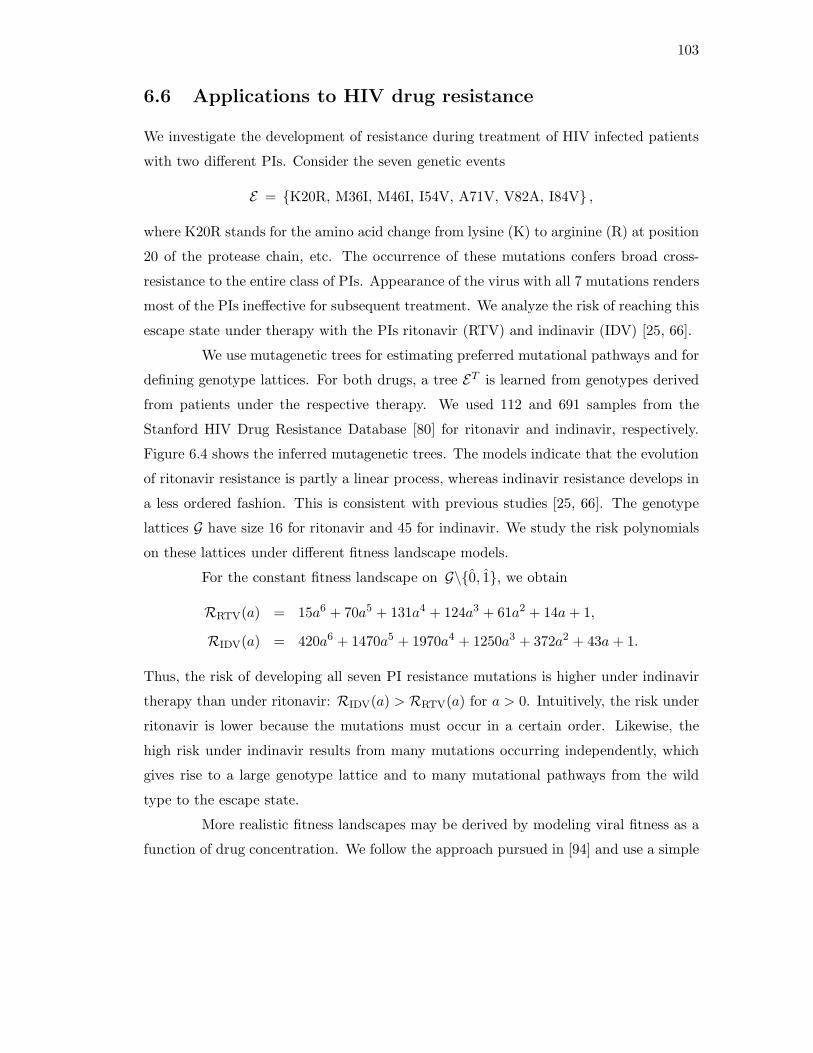
103
6.6 Applications to HIV drug resistance
We investigate the development of resistance during treatment of HIV infected patients
with two different PIs. Consider the seven genetic events
E = {K20R, M36I, M46I, I54V, A71V, V82A, I84V} ,
where K20R stands for the amino acid change from lysine (K) to arginine (R) at position
20 of the protease chain, etc. The occurrence of these mutations confers broad cross-
resistance to the entire class of PIs. Appearance of the virus with all 7 mutations renders
most of the PIs ineffective for subsequent treatment. We analyze the risk of reaching this
escape state under therapy with the PIs ritonavir (RTV) and indinavir (IDV) [25, 66].
We use mutagenetic trees for estimating preferred mutational pathways and for
defining genotype lattices. For both drugs, a tree ET is learned from genotypes derived
from patients under the respective therapy. We used 112 and 691 samples from the
Stanford HIV Drug Resistance Database [80] for ritonavir and indinavir, respectively.
Figure 6.4 shows the inferred mutagenetic trees. The models indicate that the evolution
of ritonavir resistance is partly a linear process, whereas indinavir resistance develops in
a less ordered fashion. This is consistent with previous studies [25, 66]. The genotype
lattices G have size 16 for ritonavir and 45 for indinavir. We study the risk polynomials
on these lattices under different fitness landscape models.
For the constant fitness landscape on G\{0, 1}, we obtain
RRTV(a) = 15a6 + 70a5 + 131a4 + 124a3 + 61a2 + 14a + 1,
RIDV(a) = 420a6 + 1470a5 + 1970a4 + 1250a3 + 372a2 + 43a + 1.
Thus, the risk of developing all seven PI resistance mutations is higher under indinavir
therapy than under ritonavir: RIDV(a) > RRTV(a) for a > 0. Intuitively, the risk under
ritonavir is lower because the mutations must occur in a certain order. Likewise, the
high risk under indinavir results from many mutations occurring independently, which
gives rise to a large genotype lattice and to many mutational pathways from the wild
type to the escape state.
More realistic fitness landscapes may be derived by modeling viral fitness as a
function of drug concentration. We follow the approach pursued in [94] and use a simple
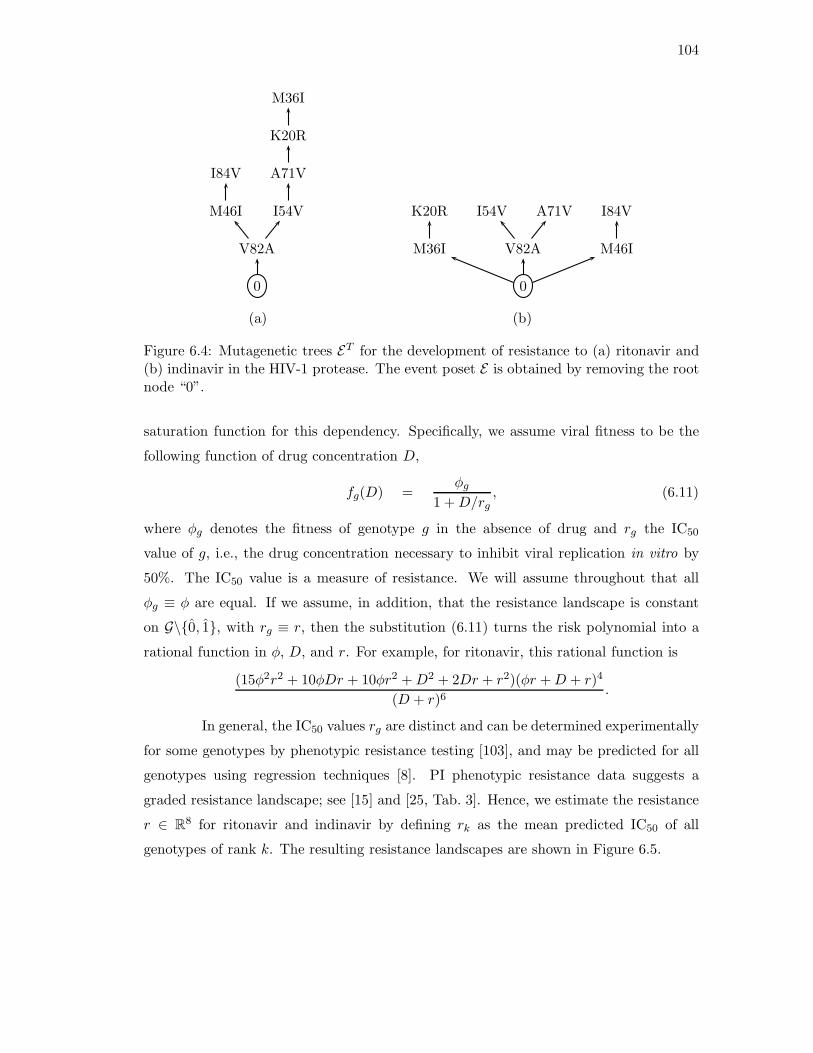
104
0
V82A
M46I
I84V
I54V
A71V
K20R
M36I
0
M36I
K20R
V82A
I54V A71V
M46I
I84V
(a) (b)
Figure 6.4: Mutagenetic trees ET for the development of resistance to (a) ritonavir and(b) indinavir in the HIV-1 protease. The event poset E is obtained by removing the rootnode “0”.
saturation function for this dependency. Specifically, we assume viral fitness to be the
following function of drug concentration D,
fg(D) =φg
1 + D/rg, (6.11)
where φg denotes the fitness of genotype g in the absence of drug and rg the IC50
value of g, i.e., the drug concentration necessary to inhibit viral replication in vitro by
50%. The IC50 value is a measure of resistance. We will assume throughout that all
φg ≡ φ are equal. If we assume, in addition, that the resistance landscape is constant
on G\{0, 1}, with rg ≡ r, then the substitution (6.11) turns the risk polynomial into a
rational function in φ, D, and r. For example, for ritonavir, this rational function is
(15φ2r2 + 10φDr + 10φr2 + D2 + 2Dr + r2)(φr + D + r)4
(D + r)6.
In general, the IC50 values rg are distinct and can be determined experimentally
for some genotypes by phenotypic resistance testing [103], and may be predicted for all
genotypes using regression techniques [8]. PI phenotypic resistance data suggests a
graded resistance landscape; see [15] and [25, Tab. 3]. Hence, we estimate the resistance
r ∈ R8 for ritonavir and indinavir by defining rk as the mean predicted IC50 of all
genotypes of rank k. The resulting resistance landscapes are shown in Figure 6.5.
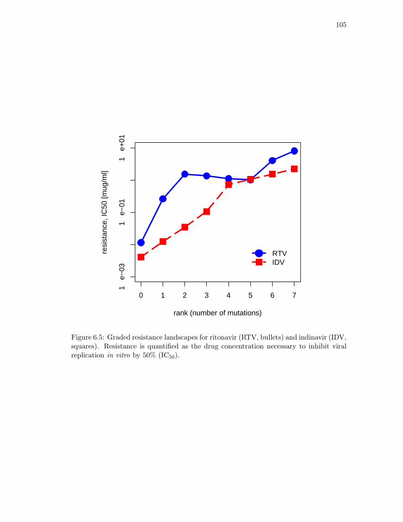
105
0 1 2 3 4 5 6 7
1 e
−03
1 e
−01
1 e
+01
rank (number of mutations)
resi
stan
ce, I
C50
[mug
/ml]
RTVIDV
Figure 6.5: Graded resistance landscapes for ritonavir (RTV, bullets) and indinavir (IDV,squares). Resistance is quantified as the drug concentration necessary to inhibit viralreplication in vitro by 50% (IC50).
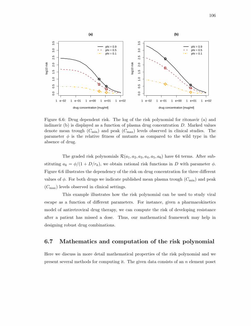
106
1 e−02 1 e−01 1 e+00 1 e+01 1 e+02
0.0
0.5
1.0
1.5
2.0
2.5
3.0
3.5
(a)
drug concentration [mug/ml]
log1
0 ris
kphi = 0.9phi = 0.5phi = 0.1
1 e−02 1 e−01 1 e+00 1 e+01 1 e+02
0.0
0.5
1.0
1.5
2.0
2.5
3.0
3.5
(b)
drug concentration [mug/ml]
log1
0 ris
k
phi = 0.9phi = 0.5phi = 0.1
Figure 6.6: Drug dependent risk. The log of the risk polynomial for ritonavir (a) andindinavir (b) is displayed as a function of plasma drug concentration D. Marked valuesdenote mean trough (Cmin) and peak (Cmax) levels observed in clinical studies. Theparameter φ is the relative fitness of mutants as compared to the wild type in theabsence of drug.
The graded risk polynomials R(a1, a2, a3, a4, a5, a6) have 64 terms. After sub-
stituting ak = φ/(1 + D/rk), we obtain rational risk functions in D with parameter φ.
Figure 6.6 illustrates the dependency of the risk on drug concentration for three different
values of φ. For both drugs we indicate published mean plasma trough (Cmin) and peak
(Cmax) levels observed in clinical settings.
This example illustrates how the risk polynomial can be used to study viral
escape as a function of different parameters. For instance, given a pharmacokinetics
model of antiretroviral drug therapy, we can compute the risk of developing resistance
after a patient has missed a dose. Thus, our mathematical framework may help in
designing robust drug combinations.
6.7 Mathematics and computation of the risk polynomial
Here we discuss in more detail mathematical properties of the risk polynomial and we
present several methods for computing it. The given data consists of an n element poset
107
E and its induced genotype lattice G, which is the distributive lattice of order ideals
in E . We assume that G has m elements, which are encoded either as subsets of E or
as binary strings in {0, 1}n. The risk polynomial is the polynomial R(G; f) in the m
unknowns fg = f(g), one for each genotype g. We are also interested in specializations
of R(G; f) obtained by setting some (or all) of the unknowns equal to each other, such
as the graded risk polynomial and the univariate risk polynomial.
Stanley’s linear algebra method
A direct method for computing the risk polynomial is given in Section 6.4. Namely, we
can set all µe equal to one in the matrix U and then compute the upper right entry
of the matrix (I − UF)−1 − I of equation (6.3). In practice, one would compute this
entry by a dynamic program which runs in time O(m2). That dynamic program is easily
derived by resolving the recursion in the last equation of the proof of Theorem 6.7.
The following alternative linear algebra technique for computing polynomials
similar to our risk polynomials was given by Stanley in [89]. Let G′ = G\{0, 1} denote
the genotype lattice with the top element 1 and the bottom element 0 removed. We
define A to be the anti-adjacency matrix of the truncated genotype lattice G′. Thus A is
the (m− 2)× (m− 2)-matrix with rows and columns indexed by G′, and whose entry in
row g and column h is 0 if g ⊂ h and is 1 otherwise. We write I for the (m−2)× (m−2)
identity matrix and F′ = diag(
f(g) | g ∈ G′)
for the (m − 2) × (m − 2)-diagonal matrix
whose entries are the fitness values. Stanley’s result reads as follows.
Theorem 6.11 (Stanley [89]). The risk polynomial R(G; f) equals the determinant of
the (m − 2) × (m − 2)-matrix I + F′ · A.
Example 6.12. Let G be the genotype lattice in Figure 6.2. Then m = 8 and I + F′ ·A
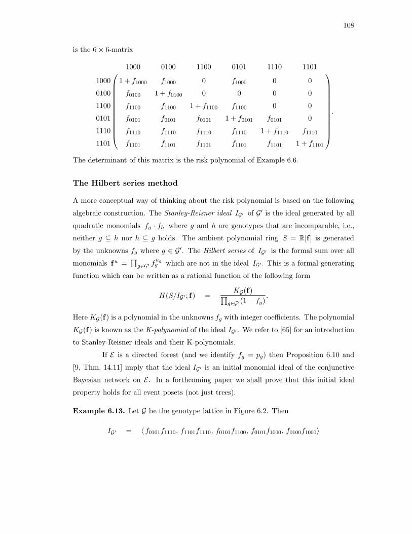
108
is the 6 × 6-matrix
1000 0100 1100 0101 1110 1101
1000 1 + f1000 f1000 0 f1000 0 0
0100 f0100 1 + f0100 0 0 0 0
1100 f1100 f1100 1 + f1100 f1100 0 0
0101 f0101 f0101 f0101 1 + f0101 f0101 0
1110 f1110 f1110 f1110 f1110 1 + f1110 f1110
1101 f1101 f1101 f1101 f1101 f1101 1 + f1101
.
The determinant of this matrix is the risk polynomial of Example 6.6.
The Hilbert series method
A more conceptual way of thinking about the risk polynomial is based on the following
algebraic construction. The Stanley-Reisner ideal IG′ of G′ is the ideal generated by all
quadratic monomials fg · fh where g and h are genotypes that are incomparable, i.e.,
neither g ⊆ h nor h ⊆ g holds. The ambient polynomial ring S = R[f ] is generated
by the unknowns fg where g ∈ G′. The Hilbert series of IG′ is the formal sum over all
monomials fu =∏
g∈G′ fugg which are not in the ideal IG′ . This is a formal generating
function which can be written as a rational function of the following form
H(S/IG′ ; f) =KG(f)
∏
g∈G′(1 − fg).
Here KG(f) is a polynomial in the unknowns fg with integer coefficients. The polynomial
KG(f) is known as the K-polynomial of the ideal IG′ . We refer to [65] for an introduction
to Stanley-Reisner ideals and their K-polynomials.
If E is a directed forest (and we identify fg = pg) then Proposition 6.10 and
[9, Thm. 14.11] imply that the ideal IG′ is an initial monomial ideal of the conjunctive
Bayesian network on E . In a forthcoming paper we shall prove that this initial ideal
property holds for all event posets (not just trees).
Example 6.13. Let G be the genotype lattice in Figure 6.2. Then
IG′ = 〈 f0101f1110, f1101f1110, f0101f1100, f0101f1000, f0100f1000〉
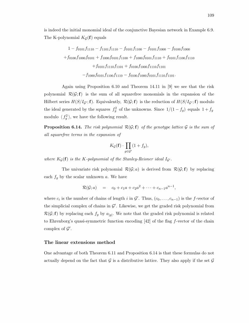
109
is indeed the initial monomial ideal of the conjunctive Bayesian network in Example 6.9.
The K-polynomial KG(f) equals
1 − f0101f1110 − f1101f1110 − f0101f1100 − f0101f1000 − f0100f1000
+f0100f1000f0101 + f1000f0101f1100 + f1000f0101f1110 + f0101f1100f1110
+f0101f1110f1101 + f0100f1000f1110f1101
−f1000f0101f1100f1110 − f0100f1000f0101f1110f1101.
Again using Proposition 6.10 and Theorem 14.11 in [9] we see that the risk
polynomial R(G; f) is the sum of all squarefree monomials in the expansion of the
Hilbert series H(S/IG′ ; f). Equivalently, R(G; f) is the reduction of H(S/IG′ ; f) modulo
the ideal generated by the squares f2g of the unknowns. Since 1/(1− fg) equals 1 + fg
modulo 〈 f2g 〉, we have the following result.
Proposition 6.14. The risk polynomial R(G; f) of the genotype lattice G is the sum of
all squarefree terms in the expansion of
KG(f) ·∏
g∈G′
(1 + fg),
where KG(f) is the K-polynomial of the Stanley-Reisner ideal IG′.
The univariate risk polynomial R(G; a) is derived from R(G; f) by replacing
each fg by the scalar unknown a. We have
R(G; a) = c0 + c1a + c2a2 + · · · + cn−1a
n−1,
where ci is the number of chains of length i in G′. Thus, (c0, . . . , cn−1) is the f -vector of
the simplicial complex of chains in G′. Likewise, we get the graded risk polynomial from
R(G; f) by replacing each fg by a|g|. We note that the graded risk polynomial is related
to Ehrenborg’s quasi-symmetric function encoding [42] of the flag f -vector of the chain
complex of G′.
The linear extensions method
One advantage of both Theorem 6.11 and Proposition 6.14 is that these formulas do not
actually depend on the fact that G is a distributive lattice. They also apply if the set G
110
of genotypes is an arbitrary poset. This is relevant for our discussion of the statistical
models in Section 6.5, where we introduced a more general class of posets Gp ⊆ {0, 1}n.
This advantage is also a disadvantage: Theorem 6.11 and Proposition 6.14 do
not give the most efficient methods for computing R(G; f) when G is the distributive
lattice induced by an event poset E . In what follows we present a specialized and more
efficient algorithm for the risk polynomial. The input to this algorithm consists of the
event poset E . It is not necessary to compute the genotype lattice G as this will be done
as a byproduct of our approach, which is to compute the risk polynomial R(G; f) directly
from E .
As before, we assume that E has n elements, and we write [n] for the linearly
ordered set {1, 2, . . . , n}. A linear extension of E is an order-preserving bijection π : E →
[n]. This means that e < e′ in E implies π(e) < π(e′). Every linear extension π : E → [n]
gives rise to an ordered list of n − 1 genotypes g(1), g(2), . . . , g(n−1) in G′ = G\{0, 1}
as follows. The genotype g(i) is the subset of E consisting of all events whose image
under π is among the first i positive integers. In symbols, g(i) = π−1({1, 2, . . . , i}). The
sequence g(1), g(2), . . . , g(n−1), derived from π, represents a mutational pathway in G.
We now fix one distinguished linear extension of E , that is, we identify the set
underlying E with [n] itself. Then a linear extension is simply any permutation π of [n]
which preserves the order relations in E . We define
f(π) =∏
i:π(i)<π(i+1)
(fg(i) + 1) ·∏
i:π(i)>π(i+1)
fg(i) , (6.12)
where i runs over {1, 2, . . . , n − 1}. Our algorithm amounts to evaluating the risk poly-
nomial by means of the following explicit summation formula.
Theorem 6.15. The risk polynomial R(G; f) equals the sum of the products f(π) where
π runs over all linear extensions of the event poset E.
Proof. The relationship between chains in G and linear extensions of E is the content
of [90, Prop. 3.5.2]. The distributive lattice G has a canonical R-labeling [90, Sec. 3.13]
which assigns to each edge of the Hasse diagram of G the corresponding element of E . In
view of this R-labeling, Exercise 59d in [90, Chap. 3] tells us that the poset G′ = G\{0, 1}
is chain-partitionable. Each product f(π) as in (6.12) is the generating function for all
111
the chains in precisely one part of that chain partition of G′. Adding up all products
gives the generating function for all chains, which is the risk polynomial.
Example 6.16. The event poset E in Figure 6.2 has five linear extensions π:
π f(π)
(1, 2, 3, 4) (1 + f1000)(1 + f1100)(1 + f1110)
(1, 2, 4, 3) (1 + f1000)(1 + f1100)f1101
(2, 1, 3, 4) f0100(1 + f1100)(1 + f1110)
(2, 1, 4, 3) f0100(1 + f1100)f1101
(2, 4, 1, 3) (1 + f0100)f0101(1 + f1101)
The sum of these five products equals the risk polynomial R(G; f).
Implementation
Pruesse and Ruskey [77] showed that the linear extensions of a poset E can be computed
in time linear in the number of linear extensions. Thus, their algorithm computes R(G; f)
in time linear in the size of the output of Theorem 6.15. That output is in factored
form (6.12) and is always more compact than the expanded risk polynomial. In this
manner, we compute the risk polynomial in time sublinear in the size of the expanded
risk polynomial.
To obtain the univariate risk polynomial, we take the sum of the terms (1 +
a)n−1−δaδ, where δ = δ(π) is the number of descents of the linear extension π. Similarly,
the graded risk polynomial R(G; a1, . . . , an−1) is found by keeping track of the descent
set of each linear extension π. We believe that this method is best possible for general
posets E . Notice that the leading term of the univariate risk polynomial is the number
of linear extensions of E , and it is #P-complete to count linear extensions [19].
When E is a directed forest, the recursive structure can be used to help compute
the risk polynomial. In this case, E is built up by the operations of disjoint union and
ordinal sum from the one element poset. For example, in the univariate case, the zeta
polynomial [90, Sec. 3.11] of G behaves nicely under these operations and can be used
112
to write down the risk polynomial. Based on these considerations, we can design an
efficient algorithm for computing the univariate risk polynomial of a directed forest.
Using the method of Theorem 6.15, we have developed software for comput-
ing risk polynomials. The input to our program is an arbitrary event poset E , and
the output is the risk polynomial, the graded risk polynomial or the univariate risk
polynomial. Optionally, the user can also input either exact fitness values or upper
and lower bounds for each fitness value. The output in this case is either the exact
risk of escape or upper and lower bounds for the risk. It is designed to integrate
with the package Mtreemix [13], allowing the user to start with data, infer a muta-
genetic tree, and then easily compute the risk polynomial. Our software is available at
http://bio.math.berkeley.edu/riskpoly/We use the algorithm of [101] for comput-
ing linear extensions. Although this algorithm isn’t asymptotically optimal (see [77]), it
is simple to implement and efficient in practice.
6.8 Discussion
We have presented a computational framework for assessing the risk of escape of an
evolving population of pathogens. The risk of escape is the probability that the popula-
tion reaches an escape state before extinction. In virus transmissions, for example, this
probability is the chance of survival in the new host. In the situation of antiretroviral
therapy, the risk of escape is the probability of therapy failure due to the development
of drug resistance.
The general setup we consider for computing the risk of escape includes an
event poset, a fitness landscape on its induced genotype lattice, and a branching process
on this lattice. The event poset E consists of all mutational events that can occur and
encodes the constraints which apply to their order of occurrence. From this structure the
genotype space G is obtained by considering all mutational pathways that respect the
order constraints. This natural construction endows G with the mathematical structure
of a distributive lattice. The risk polynomial, the crucial factor in computing the risk
of escape, turns out to coincide with the chain polynomial of the genotype lattice. We
have presented methods from algebraic combinatorics that exploit this connection and
113
that result in efficient algorithms.
The space of genotypes may also be inferred from observed genotype data us-
ing statistical model selection tools. We have identified a class of Bayesian network
models, the conjunctive Bayesian networks, whose support induces a genotype lattice.
Mutagenetic tree models arise as important special cases. Here, both statistical model
selection and risk computation are particularly efficient, and readily available with ex-
isting software [13] coupled with our implementation of the linear extensions method
(Theorem 6.15).
We have focused on the dependency of the risk polynomial on the fitness land-
scape and considered throughout a homogeneous wild type population prior to interven-
tion. However, the risk of escape is calculated similarly for a quasispecies distribution at
the time of intervention. In fact, this involves computing the risk polynomial of the prior
fitness landscape [54]. In contrast, the branching process model can not account for re-
combination, horizontal gene transfer, or frequency dependent selection, since evolution
is assumed to take place in multiple lineages independently.
The main challenge in using our method to compute the risk of escape from
antiretroviral therapy lies in accurately modeling the fitness landscape. The dependency
(6.11) of the fitness on drug concentration may be improved by experimentally deter-
mined viral replicative capacities in the absence of drugs. An alternative approach to
derive a fitness landscape for HIV-1 proteases is based on estimating the binding affin-
ity of the drug to the mutant protease, and the mutant’s ability to cleave its natural
substrates [82]. These calculations are based on simplified molecular modeling tech-
niques. The resulting fitness landscape does not account for different drug levels, but it
is independent of experimental resistance and fitness data.
Escape from indinavir and ritonavir therapy may in some cases involve muta-
tions other than the seven we considered, although those are the most frequent mutations
observed after therapy failure [25, 66]. On the other hand, viral escape might be accom-
plished with genotypes that harbor fewer than all of the mutations. Thus it would be
desirable to compute the risk of reaching any of several escape states, rather than only
the 11 · · · 1 type. This computation will involve similar techniques to those presented in
Sections 6.4 and 6.7.

114
Finally, the PIs form only one out of four distinct classes of antiretroviral drugs
that are in current clinical use. The standard of care is combination therapy with at
least three different drugs from two different drug classes. Modeling the fitness landscape
of combination therapy in terms of viral drug resistance and drug exposure is even
more challenging, but can eventually help in designing optimal antiretroviral therapies.
Algebraic combinatorics offers tools for the mathematical analysis of these biomedical
problems.

115
Bibliography
[1] Jameel Al-Aidroos and Sagi Snir. Analysis of point mutations in vertebrate
genomes. In L. Pachter and B. Sturmfels, editors, Algebraic Statistics for Computa-
tional Biology, chapter 21, pages 375–386. Cambridge University Press, Cambridge,
UK, 2005.
[2] ES Allman and JA Rhodes. Phylogenetic invariants for the general Markov model
of sequence mutation. Mathematical Biosciences, 186(2):113–144, 2003.
[3] ES Allman and JA Rhodes. Phylogenetic ideals and varieties for the general
Markov model. http://arxiv.org/abs/math.AG/0410604, 2004.
[4] ES Allman and JA Rhodes. Quartets and parameter recovery for the general
Markov model of sequence mutation. AMRX Applied Mathematics Research Ex-
press, 2004(4):107–131, 2004.
[5] M Ashburner, CA Ball, JA Blake, D Botstein, H Butler, JM Cherry, K Dolinski,
SS Dwight, JT Eppig, MA Harris, et al. Gene Ontology: tool for the unification
of biology. The Gene Ontology Consortium. Nature Genetics, 25:25–29, 2000.
[6] K.B. Athreya and P.E. Ney. Branching processes. Dover, Mineola, New York, 1972.
[7] Matthias Beck and Dennis Pixton. The Ehrhart polynomial of the Birkhoff poly-
tope. Discrete Comput. Geom., 30(4):623–637, 2003.
[8] Niko Beerenwinkel, Martin Daumer, Mark Oette, Klaus Korn, Daniel Hoffmann,
Rolf Kaiser, Thomas Lengauer, Joachim Selbig, and Hauke Walter. Geno2pheno:

116
Estimating phenotypic drug resistance from HIV-1 genotypes. Nucleic Acids Res,
31(13):3850–3855, Jul 2003.
[9] Niko Beerenwinkel and Mathias Drton. Mutagenetic tree models. In L. Pachter and
B. Sturmfels, editors, Algebraic Statistics for Computational Biology, chapter 14,
pages 278–290. Cambridge University Press, Cambridge, UK, 2005.
[10] Niko Beerenwinkel, Nicholas Eriksson, and Bernd Sturmfels. Evolution on dis-
tributive lattices. Journal of Theoretical Biology, 2006.
[11] Niko Beerenwinkel, Lior Pachter, and Bernd Sturmfels. Epistasis and shapes of
fitness landscapes. http://www.arxiv.org/abs/q-bio.PE/0603034, 2006.
[12] Niko Beerenwinkel, Jorg Rahnenfuhrer, Martin Daumer, Daniel Hoffmann, Rolf
Kaiser, Joachim Selbig, and Thomas Lengauer. Learning multiple evolutionary
pathways from cross-sectional data. J Comput Biol, 12(6):584–598, 2005. RE-
COMB 2004.
[13] Niko Beerenwinkel, Jorg Rahnenfuhrer, Rolf Kaiser, Daniel Hoffmann, Joachim
Selbig, and Thomas Lengauer. Mtreemix: a software package for learning and
using mixture models of mutagenetic trees. Bioinformatics, 21(9):2106–2107, May
2005.
[14] G Bejerano, M Pheasant, I Makunin, S Stephen, WJ Kent, JS Mattick, and
D Haussler. Ultraconserved elements in the human genome. Science, 304:1321–
1325, 2004.
[15] B. Berkhout. HIV-1 evolution under pressure of protease inhibitors: Climbing the
stairs of viral fitness. J. Biomed. Sci., 6:298–305, 1999.
[16] Louis J. Billera, Susan P. Holmes, and Karen Vogtmann. Geometry of the space
of phylogenetic trees. Adv. in Appl. Math., 27(4):733–767, 2001.
[17] D Boffelli, MA Nobrega, and EM Rubin. Comparative genomics at the vertebrate
extremes. Nature Reviews Genetics, 5:456–465, 2004.
117
[18] Nicolas Bray and Lior Pachter. MAVID: constrained ancestral alignment of mul-
tiple sequences. Genome Research, 14(4):693–9, 2004.
[19] Graham Brightwell and Peter Winkler. Counting linear extensions. Order,
8(3):225–242, 1991.
[20] M Brudno, S Malde, A Poliakov, C Do, O Couronne, I Dubchak, and S Batzoglou.
Global alignment: finding rearrangements during alignment. Special issue on the
Proceedings of the ISMB 2003, Bioinformatics, 19:54i–64i, 2003.
[21] Marta Casanellas, Luis David Garcia, and Seth Sullivant. Catalog of small trees.
In L. Pachter and B. Sturmfels, editors, Algebraic Statistics for Computational
Biology, chapter 15, pages 291–304. Cambridge University Press, Cambridge, UK,
2005.
[22] J.A. Cavender and J. Felsenstein. Invariants of phylogenies: A simple case with
discrete states. J. Classif., 4:57–71, 1987.
[23] Franois Clavel and Allan J. Hance. HIV drug resistance. N. Engl. J. Med.,
350(10):1023–1035, Mar 2004.
[24] S. Collart, M. Kalkbrener, and D. Mall. Converting bases with the Grobner walk.
J. Symbolic Comput., 24(3-4):465–469, 1997. Computational algebra and number
theory (London, 1993).
[25] J.H. Condra, D.J. Holder, W.A. Schleif, O.M. Blahy, R.M. Danovich, L.J. Gabryel-
ski, D.J. Graham, D. Laird, J.C. Quintero, A. Rhodes, H.L. Robbins, E. Roth,
M. Shivaprakash, T. Yang, J.A. Chodakewitz, P.J. Deutsch, R.Y. Leavitt, F.E.
Massari, J.W. Mellors, K.E. Squires, R.T. Steigbigel, H. Teppler, and E.A. Emini.
Genetic correlates of in vivo viral resistance to indinavir, a human immunodefi-
ciency virus type 1 protease inhibitor. J. Virol., 70(12):8270–8276, 1996.
[26] ENCODE Project Consortium. The ENCODE (ENCyclopedia Of DNA Elements)
Project. Science, 306(5696):636–40, 2004.
118
[27] David Cox, John Little, and Donal O’Shea. Ideals, varieties, and algorithms.
Undergraduate Texts in Mathematics. Springer-Verlag, New York, second edition,
1997. An introduction to computational algebraic geometry and commutative
algebra.
[28] J.A. De Loera, D. Haws, R. Hemmecke, P. Huggins, J. Tauzer, and R. Yoshida. A
user’s guide for latte v1.1. Available at http://www.math.ucdavis.edu/∼latte/,
2003.
[29] W.L. DeLano. The PyMOL molecular graphics system. Available at
http://www.pymol.org, 2002.
[30] JW Demmel. Applied Numerical Linear Algebra. Society for Industrial and Applied
Mathematics (SIAM), Philadelphia, PA, 1997.
[31] R Desper, F Jiang, O-P Kallioniemi, H Moch, CH Papadimitriou, and AA Schaffer.
Inferring tree models for oncogenesis from comparative genome hybridization data.
Journal of Computational Biology, 6(1):37–51, 1999.
[32] C Dewey. MERCATOR: multiple whole-genome orthology map construction.
Available at http://hanuman.math.berkeley.edu/∼cdewey/mercator/, 2005.
[33] Colin Dewey, Peter Huggins, Kevin Woods, Lior Pachter, and Bernd Sturmfels.
Parametric alignment of drosophila genomes. PLoS Computational Biology, 2006.
To appear.
[34] Persi Diaconis. Group Representations in Probability and Statistics, volume 11 of
IMS Lecture Series. Institute of Mathematical Statistics, 1988.
[35] Persi Diaconis. A generalization of spectral analysis with application to ranked
data. Ann. Statist., 17(3):949–979, 1989.
[36] Persi Diaconis and Bradley Efron. Testing for independence in a two-way table:
new interpretations of the chi-square statistic. Ann. Statist., 13(3):845–913, 1985.
[37] Persi Diaconis and Nicholas Eriksson. Markov bases for noncommutative Fourier
analysis of ranked data. J. Symbolic Comput., 41(2):182–195, 2006.
119
[38] Persi Diaconis and D. Freedman. Partial exchangeability and sufficiency. In J.K.
Ghosh and J. Roy, editors, Statistics: Applications and New Directions, pages
205–236, Calcutta, 1984. Indian Statistical Institute.
[39] Persi Diaconis and Bernd Sturmfels. Algebraic algorithms for sampling from con-
ditional distributions. Ann. Statist., 26(1):363–397, 1998.
[40] Mathias Drton, Nicholas Eriksson, and Garmay Leung. Ultra-conserved elements
in vertebrate and fly genomes. In L. Pachter and B. Sturmfels, editors, Alge-
braic Statistics for Computational Biology, chapter 22, pages 387–402. Cambridge
University Press, Cambridge, UK, 2005.
[41] Rick Durrett. Genome rearrangement. In Statistical methods in molecular evolu-
tion, Stat. Biol. Health, pages 307–323. Springer, New York, 2005.
[42] Richard Ehrenborg. On posets and Hopf algebras. Adv. Math., 119(1):1–25, 1996.
[43] Nicholas Eriksson. Toric ideals of homogeneous phylogenetic models. In ISSAC
2004, pages 149–154. ACM, New York, 2004.
[44] Nicholas Eriksson. Tree construction using singular value decompsition. In
L. Pachter and B. Sturmfels, editors, Algebraic Statistics for Computational Bi-
ology, chapter 19, pages 347–358. Cambridge University Press, Cambridge, UK,
2005.
[45] Nicholas Eriksson, Kristian Ranestad, Bernd Sturmfels, and Seth Sullivant. Phy-
logenetic algebraic geometry. In C. Ciliberto, A. Geramita, B. Harbourne, R-M.
Roig, and K. Ranestad, editors, Projective varieties with unexpected properties,
pages 237–255. Walter de Gruyter GmbH & Co. KG, Berlin, 2005.
[46] Joseph Felsenstein. Inferring Phylogenies. Sinauer Associates, Sunderland, 2003.
[47] Joseph Felsenstein. Phylip (phylogeny inference package) version 3.6. Available at
http://evolution.genetics.washington.edu/phylip.html, 2005.
[48] Ronald A. Fisher. Statistical methods for research workers. Hafner Publishing Co.,
New York, 1973.

120
[49] A Frieze, R Kannan, and S Vempala. Fast Monte Carlo algorithms for low rank
approximation. In 39th Symposium on Foundations of Computing, pages 370–378,
1998.
[50] William Fulton. Introduction to toric varieties, volume 131 of Annals of Mathe-
matics Studies. Princeton University Press, Princeton, NJ, 1993. The William H.
Roever Lectures in Geometry.
[51] Luis David Garcia, Michael Stillman, and Bernd Sturmfels. Algebraic geometry
of Bayesian networks. Journal of Symbolic Computation, 39/3-4:331–355, 2004.
Special issue on the occasion of MEGA 2003.
[52] G.-M. Greuel, G. Pfister, and H. Schonemann. Singular 3.0. A Computer Algebra
System for Polynomial Computations, Centre for Computer Algebra, University of
Kaiserslautern, 2005. http://www.singular.uni-kl.de.
[53] Raymond Hemmecke and Ralf Hemmecke. 4ti2 version 1.1—computation of Hilbert
bases, Graver bases, toric Grobner bases, and more. Available at www.4ti2.de,
September 2003.
[54] Yoh Iwasa, Franziska Michor, and Martin A. Nowak. Evolutionary dynamics of
escape from biomedical intervention. Proc Biol Sci, 270(1533):2573–2578, Dec
2003.
[55] Yoh Iwasa, Franziska Michor, and Martin A. Nowak. Evolutionary dynamics of
invasion and escape. J Theor Biol, 226(2):205–214, Jan 2004.
[56] Anders N. Jensen. Gfan, a software system for Grobner fans. Available at
http://home.imf.au.dk/ajensen/software/gfan/gfan.html.
[57] Anders N. Jensen. Cats, a software system for toric state polytopes. Available at
http://www.soopadoopa.dk/anders/cats/cats.html, 2003.
[58] Eric Kuo. Geometry of Markov chains. In L. Pachter and B. Sturmfels, editors,
Algebraic Statistics for Computational Biology, chapter 10, pages 226–236. Cam-
bridge University Press, 2005.
121
[59] JA Lake. A rate-independent technique for analysis of nucleaic acid sequences:
evolutionary parsimony. Molecular Biology and Evolution, 4:167–191, 1987.
[60] J. M. Landsberg and L. Manivel. On the ideals of secant varieties of Segre varieties.
Found. Comput. Math., 4(4):397–422, 2004.
[61] SL Lauritzen. Graphical models, volume 17 of Oxford Statistical Science Series.
The Clarendon Press Oxford University Press, New York, 1996. Oxford Science
Publications.
[62] Jun Liu. Monte Carlo techniques in scientific computing. Springer, New York,
2001.
[63] J. Marden. Analyzing and modeling rank data. Chapman and Hall, London, 1995.
[64] Jon D. McAuliffe, Lior Pachter, and Michael I. Jordan. Multiple-sequence func-
tional annotation and the generalized hidden Markov phylogeny. Bioinformatics,
20(12):1850–60, 2004.
[65] Ezra Miller and Bernd Sturmfels. Combinatorial commutative algebra, volume 227
of Graduate Texts in Mathematics. Springer-Verlag, New York, 2005.
[66] A. Molla, M. Korneyeva, Q. Gao, S. Vasavanonda, P. J. Schipper, H. M. Mo,
M. Markowitz, T. Chernyavskiy, P. Niu, N. Lyons, A. Hsu, G. R. Granneman, D. D.
Ho, C. A. Boucher, J. M. Leonard, D. W. Norbeck, and D. J. Kempf. Ordered
accumulation of mutations in HIV protease confers resistance to ritonavir. Nat
Med, 2(7):760–766, Jul 1996.
[67] SY Ng, P Gunning, R Eddy, P Ponte, J Leavitt, T Shows, and L Kedes. Evolution
of the functional human beta-actin gene and its multi-pseudogene family: conser-
vation of noncoding regions and chromosomal dispersion of pseudogenes. Molecular
and Cellular Biology, 5:2720–2732, 1985.
[68] MA Nobrega, I Ovcharenko, V Afzal, and EM Rubin. Scanning human gene deserts
for long-range enhancers. Science, 302(5644):413, 2003.
[69] M.A. Nowak and R.M. May. Virus dynamics. Oxford University Press, 2000.

122
[70] S Ota and WH Li. Njml: A hybrid algorithm for the neighbor-joining and maxi-
mum likelihood methods. Molecular Biology and Evolution, 17(9):1401–1409, 2000.
[71] Lior Pachter and Bernd Sturmfels. Parametric inference for biological sequence
analysis. Proc. Natl. Acad. Sci. USA, 101(46):16138–16143 (electronic), 2004.
[72] Lior Pachter and Bernd Sturmfels. Tropical geometry of statistical models. Proc.
Natl. Acad. Sci. USA, 101(46):16132–16137 (electronic), 2004.
[73] Lior Pachter and Bernd Sturmfels. Algebraic Statistics for Computational Biology.
Cambridge University Press, Cambridge, UK, 2005.
[74] Lior Pachter and Bernd Sturmfels. The mathematics of phylogenomics. SIAM
Review, 2006.
[75] T Peters, R Dildrop, K Ausmeier, and U Ruther. Organization of mouse iroquois
homeobox genes in two clusters suggests a conserved regulation and function in
vertebrate development. Genome Research, 10:1453–1462, 2000.
[76] TD Pollard. Genomics, the cytoskeleton and motility. Nature, 409:842–843, 2001.
[77] Gara Pruesse and Frank Ruskey. Generating linear extensions fast. SIAM J.
Comput., 23(2):373–386, 1994.
[78] A Rambaut and NC Grassly. Seq-Gen: An application for the Monte Carlo simu-
lation of DNA sequence evolution along phylogenetic trees. Comput. Appl. Biosci.,
13:235–238, 1997.
[79] Christian M. Reidys and Peter F. Stadler. Combinatorial landscapes. SIAM Re-
view, 44:3–54, 2002.
[80] Soo-Yon Rhee, Matthew J Gonzales, Rami Kantor, Bradley J Betts, Jaideep Rav-
ela, and Robert W Shafer. Human immunodeficiency virus reverse transcriptase
and protease sequence database. Nucleic Acids Res, 31(1):298–303, Jan 2003.
[81] Ruy M. Ribeiro and Sebastian Bonhoeffer. Production of resistant HIV mutants
during antiretroviral therapy. PNAS, 97(14):7681–7686, 2000.
123
[82] C.D. Rosin, R.K. Belew, G.M. Morris, A.J. Olson, and D.S. Goodsell. Coevolu-
tionary analysis of resistance-evading peptidomimetic inhibitors of HIV-1 protease.
Proc. Natl. Acad. Sci. U.S.A., 96:1369–1374, 1999.
[83] N Saitou and M Nei. The neighbor-joining method: a new method for reconstruct-
ing phylogenetic trees. Mol Biol Evol, 4:406–425, 1987.
[84] A Sandelin, P Bailey, S Bruce, PG Engstrom, JM Klos, WW Wasserman, J Eric-
son, and B Lenhard. Arrays of ultraconserved non-coding regions span the loci of
key developmental genes in vertebrate genomes. BMC Genomics, 5:99, 2004.
[85] D Sankoff and M Blanchette. Comparative genomics via phylogenetic invariants
for Jukes-Cantor semigroups. In Stochastic models (Ottawa, ON, 1998), volume 26
of Proceedings of the International Conference on Stochstic Models, pages 399–418.
American Mathematical Society, Providence, RI, 2000.
[86] Charles Semple and Mike Steel. Phylogenetics, volume 24 of Oxford Lecture Series
in Mathematics and its Applications. Oxford University Press, Oxford, 2003.
[87] A Siepel and D Haussler. Combining phylogenetic and hidden markov models in
biosequence analysis. Journal of Computational Biology, 11:413–428, 2004.
[88] A. Silverberg. Statistical models for q-permutations. Proc Biopharm. Sec. Amer.
Statist. Assoc., pages 107–112, 1984.
[89] Richard P. Stanley. A matrix for counting paths in acyclic digraphs. J. Combin.
Theory Ser. A, 74(1):169–172, 1996.
[90] Richard P. Stanley. Enumerative combinatorics. Vol. 1, volume 49 of Cambridge
Studies in Advanced Mathematics. Cambridge University Press, Cambridge, 1997.
[91] M. Steel, L. Szekely, P. Erdos, and P. Waddell. A complete family of phylogenetic
invariants for any number of taxa under Kimura’s 3st model. New Zealand Journal
of Botany, 31:289–296, 1993.
[92] M A Steel and Y X Fu. Classifying and counting linear phylogenetic invariants for
the Jukes-Cantor model. J Comput Biol, 2(1):39–47, Spring 1995.
124
[93] H. Stern. Probability models on rankings and the electoral process. In M. Fligner
and J. Verducci, editors, Probability models and statistical analyses for ranking
data, pages 173–195. Springer, 1993.
[94] N.I. Stilianakis, C.A. Boucher, M.D. De Jong, R. Van Leeuwen, R. Schuurman,
and R.J. De Boer. Clinical data sets of human immunodeficiency virus type 1
reverse transcriptase resistant muatnts explained by a mathematical model. J.
Virol., 71(1):161–168, 1997.
[95] V Strassen. Rank and optimal computation of generic tensors. Linear Algebra
Appl., 52/53:645–685, 1983.
[96] K Strimmer and A von Haeseler. Quartet puzzling: A quartet maximum likeli-
hood method for reconstructing tree topologies. Molecular Biology and Evolution,
13:964–969, 1996.
[97] B Sturmfels and S Sullivant. Toric ideals of phylogenetic invariants. Journal of
Computational Biology, 12:204–228, 2005.
[98] Bernd Sturmfels. Grobner bases and convex polytopes, volume 8 of University
Lecture Series. American Mathematical Society, Providence, RI, 1996.
[99] Bernd Sturmfels. Equations defining toric varieties. In Algebraic geometry—Santa
Cruz 1995, volume 62 of Proc. Sympos. Pure Math., pages 437–449. Amer. Math.
Soc., Providence, RI, 1997.
[100] J. H. van Lint and R. M. Wilson. A course in combinatorics. Cambridge University
Press, Cambridge, second edition, 2001.
[101] Yaakov L. Varol and Doron Rotem. An algorithm to generate all topological sorting
arrangements. Comput. J., 24(1):83–84, 1981.
[102] J. Verducci. Discriminating between two probabilities on the basis of ranked pref-
erences. PhD thesis, Stanford University, 1982.
125
[103] H. Walter, B. Schmidt, K. Korn, A. M. Vandamme, T. Harrer, and K. Uberla.
Rapid, phenotypic HIV-1 drug sensitivity assay for protease and reverse transcrip-
tase inhibitors. J. Clin. Virol., 13:71–80, 1999.
[104] Michael S. Waterman. Applications of combinatorics to molecular biology. In
Handbook of combinatorics, Vol. 1, 2, pages 1983–2001. Elsevier, Amsterdam, 1995.
[105] C.O. Wilke. Probability of fixation of an advantageous mutant in a viral quasis-
pecies. Genetics, 163:467–474, 2003.
[106] A Woolfe, M Goodson, DK Goode, P Snell, GK McEwen, T Vavouri, SF Smith,
P North, H Callaway, K Kelly, et al. Highly conserved non-coding sequences are
associated with vertebrate development. PLoS Biology, 3:7, 2005.
[107] Z Yang. PAML: A program package for phylogenetic analysis by maximum likeli-
hood. CABIOS, 15:555–556, 1997.