Algebraic geometric codes on curves and surfacesalgant.eu/documents/theses/zampolini.pdf · The theory of algebraic geometric codes on curves has been deeply stud-ied during the ’80s

Algebraic geometric codeson curves and surfaces

Paolo Zampolini

Master Program in MathematicsFaculty of Science

University of Padova,Italy.

Supervisor: prof. Luca Barbieri Viale

Department of Pure and Applied Mathematics,University of Padova.

Italy

Padova, 22nd March 2007

“The main application of Pure Mathematics is to make you happy”

H.W. Lenstra, Leiden, November 2005

Contents

Introduction 6

1 Basic notions of coding theory 7

2 Algebraic geometric codes on curves 112.1 AG codes . . . . . . . . . . . . . . . . . . . . . . . . . . . . . 112.2 Dual AG codes . . . . . . . . . . . . . . . . . . . . . . . . . . 122.3 Rational points on curves and lower bounds . . . . . . . . . . 15

3 Decoding methods 213.1 SV-algorithm . . . . . . . . . . . . . . . . . . . . . . . . . . . 213.2 A cubic curve . . . . . . . . . . . . . . . . . . . . . . . . . . . 243.3 The Duursma algorithm . . . . . . . . . . . . . . . . . . . . . 273.4 Example . . . . . . . . . . . . . . . . . . . . . . . . . . . . . . 343.5 Another example: the Klein quartic . . . . . . . . . . . . . . 36

4 Codes over higher dimensional varieties 414.1 Sheaves of modules . . . . . . . . . . . . . . . . . . . . . . . . 414.2 Divisors . . . . . . . . . . . . . . . . . . . . . . . . . . . . . . 454.3 Definition of AG codes on varieties . . . . . . . . . . . . . . . 48

5 Codes on surfaces 505.1 Ample and very ample invertible sheaves . . . . . . . . . . . . 505.2 Arithmetic and geometric genus of varieties . . . . . . . . . . 515.3 Basic properties of surfaces . . . . . . . . . . . . . . . . . . . 545.4 Parameters of codes on surfaces . . . . . . . . . . . . . . . . . 56

6 Codes on ruled surfaces 596.1 The projective space bundle . . . . . . . . . . . . . . . . . . . 596.2 Ruled surfaces . . . . . . . . . . . . . . . . . . . . . . . . . . 606.3 Parameters of codes on ruled surfaces . . . . . . . . . . . . . 636.4 Codes on rational ruled surfaces . . . . . . . . . . . . . . . . . 646.5 Computing the dimension in the decomposable case . . . . . 656.6 Computing the dimension in the general case . . . . . . . . . 666.7 Ruled surfaces over elliptic curves . . . . . . . . . . . . . . . . 706.8 Conclusion and open problems . . . . . . . . . . . . . . . . . 75

6 INTRODUCTION

Introduction

One of the main developments in the coding theory in the ’80s was theintroduction of algebraic geometric codes, due to the russian mathematicianand engineer Goppa. His main idea was to associate linear codes to divisorson curves.

In 1982 Tsfasman, Vladut and Zink used this new class of codes to provethe existence of codes with better parameters than the ones ensured by theGilbert-Varshamow bound.

The theory of algebraic geometric codes on curves has been deeply stud-ied during the ’80s and the ’90s and now we can consider it to be well-knownby the mathematical community. Nowadays most of the works about alge-braic geometric codes on curves concern the search of a faster decoding algo-rithm. Indeed at the present times other codes with more efficient decodingalgorithms are preferred to algebraic geometric codes in the applications.

In 1991 Tsfasman and Vladut generalized Goppa’s idea and defined al-gebraic geometric codes on varieties.

Nevertheless, the first publication about codes on higher dimensional va-rieties is dated 2001. Hansen’s PhD thesis opened a new interesting researchfield, combining both coding theory and the geometry of varieties.

The aim of this work is to introduce the theory of algebraic geometric codeson curves and present the recent progresses about codes on higher dimen-sional varieties.

In the first section we recall the elementary notions of coding theory.The second section regards algebraic geometric codes on curves with par-

ticular attention to the connection between them and the Gilbert-Varshamovbound, while the third one contains two decoding algorithms for codes oncurves.

We introduce in the fourth section codes on higher dimensional varietiesand then we follow Hansen and Zarzar’s works to study codes on surfaces.

Lastly we focus on Lomont’s PhD thesis about codes on ruled surfacesand we try to solve a problem left open in it.

In sections 2 and 3 the language of classical algebraic geometry is as-sumed to be known, while in the last three sections we also recall the re-quired notions of scheme theory. Proofs are often omitted but we try todefine almost every geometric object we use.

7

1 Basic notions of coding theory

Definition 1.1 Let Fq be a field with q elements. An error correctingcode is a subset C of Fn

q . C is said linear if it is a sub-vector space of Fnq .

In practice most of the codes are linear codes and they are used to transformwords of length k < n (with letters in the alphabet Fq) to words of length nin order to find and correct errors happened during the transmission. Theelements of the code are called words.

Let x,y ∈ Fnq . The Hamming distance (or, simply, distance) is defined as

d(x, y) := #i | 1 ≤ i ≤ n, xi 6= yi.

d really defines a metric on Fnq . The minimum distance d of a code C is

d = d(C) := mind(x, y) | x, y ∈ C, x 6= y.

It is immediate to see that the minimum distance of a linear code correspondsto the minimum weight

w = w(C) := minwt(x) | x ∈ C, x 6= 0,

where wt(x) := #i | xi 6= 0. Let us indicate with (n,M, d) a code oflength n, M words and distance d, while an [n, k, d]-code is a linear code oflength n, dimension k and distance d.

The decoding of a message respects the so-called maximum-likelihood-decoding principle, i.e. we suppose that, during the transmission, the small-est number of errors occurred. The received vector y ∈ Fq

n is interpretedas the code word x ∈ C such that wt(x− y) is as small as possible. Thus itis clear that a code with minimum distance d is able to find every error ofweight e < d and correct every error of weight not bigger than e = bd−1

2 c. Itfollows trivially from the triangular inequality that spheres of radius e andcenter in a code word are disjoint. A code with distance d = 2e+1 is said tobe perfect if such spheres cover Fn

q . Hence, for a perfect code, every y ∈ Fnq

has distance less or equal e from a unique code word.

The most immediate relation between the parameters of a code is calledsingleton bound.

Proposition 1.1 (Singleton bound) Let C be an (n,M, d)−code. ThenMqd−1 ≤ qn.

The proposition can be proved just by counting the elements of Fnq that

belong to the disjoint spheres of radius e = bd−12 c and with a code word as

8 1 BASIC NOTIONS OF CODING THEORY

center. A code whose parameters satisfy the equality in the previous propo-sition is called MDS (maximum-distance-separable). We remark that, fora [n, k, d]-code, the singleton bound can be written as d + k ≤ n + 1.

A fundamental role in the development of coding theory is due to Shan-non’s work ([20]) and, in particular, to his famous theorem. Suppose wehave to transmit a message through a channel where the probability of re-ceiving a wrong digit is p and the probability of transmitting a wrong symbolis the same for every symbol (such a channel is called uniform). Further-more suppose we use a code C formed by M words x1, · · · , xM which occurwith the same probability. Let Pi be the probability of not being able todecode exactly xi according to the maximum-likelihood-decoding principle.In this case the average probability of wrongly decoding a code in C isPC =

∑ni=1

PiM . Hence a code with good properties is a a code such that PC

is minimum. Let P ∗(M,n, p) be the minimum PC for C running over all the(M, n)-codes and R = logq M

n the so-called information rate.

Theorem 1.1 (Shannon) There exists a function c, called channel ca-pacity, depending only on q and p, such that, if 0 < R < c and Mn = qbRnc,then limn→+∞ P ∗(Mn, n, p) = 0.

By Shannon’s theorem, for R in an interval depending only on the trans-mission channel, among the codes with the same information rate, the goodones are those with n big. This is a good motivation to look for long codesand to study the asymptotical behavior of codes in the same class, letting nchange.

During the transmission of a word of length n through a channel withprobability p, we expect an average of pn errors. Hence we need a codewith minimum distance d > 2pn. We therefore require that d grows at leastproportionally to n.

Let δ = dn , Aq(n, d) = maxM | there exists a (n,M, d)-code over Fq. We

now define the function α:

α(δ) = lim supn→+∞

logq Aq(n, bδnc)n

,

which is an important and widely studied object of the coding theory. Thuswe are interested in studying, for a fixed δ, what the best possible infor-mation rate for a code of length n is, and then letting n go to infinity, assuggested by Shannon’s theorem. The easiest (and the least precise) amongthose upper bounds for α is a direct consequence of singleton bound.

Theorem 1.2 For δ ∈ [0, 1], we have α(δ) ≤ 1− δ.

9

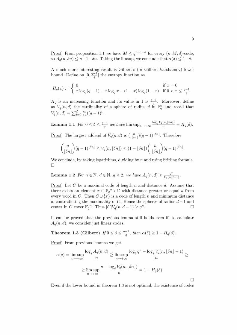
Proof: From proposition 1.1 we have M ≤ qn+1−d for every (n,M, d)-code,so Aq(n, δn) ≤ n+1−δn. Taking the limsup, we conclude that α(δ) ≤ 1−δ.

A much more interesting result is Gilbert’s (or Gilbert-Varshamov) lowerbound. Define on [0, q−1

q ] the entropy function as

Hq(x) :=

0 if x = 0x logq(q − 1)− x logq x− (1− x) logq(1− x) if 0 < x ≤ q−1

q

Hq is an increasing function and its value in 1 is q−1q . Moreover, define

as Vq(n, d) the cardinality of a sphere of radius d in Fnq and recall that

Vq(n, d) =∑d

i=0

(ni

)(q − 1)i.

Lemma 1.1 For 0 ≤ δ ≤ q−1q we have lim supn→+∞

logq Vq(n,bnδc)n = Hq(δ).

Proof: The largest addend of Vq(n, d) is(

nbδnc

)(q − 1)bδnc. Therefore

(n

bδnc)

(q − 1)bδnc ≤ Vq(n, bδnc) ≤ (1 + bδnc)(

n

bδnc)

(q − 1)bδnc.

We conclude, by taking logarithms, dividing by n and using Stirling formula.¤

Lemma 1.2 For n ∈ N, d ∈ N, q ≥ 2, we have Aq(n, d) ≥ qn

Vq(n,d−1) .

Proof: Let C be a maximal code of length n and distance d. Assume thatthere exists an element x ∈ Fq

n \ C with distance greater or equal d fromevery word in C. Then C ∪x is a code of length n and minimum distanced, contradicting the maximality of C. Hence the spheres of radius d− 1 andcenter in C cover Fq

n. Thus |C|Vq(n, d− 1) ≥ qn. ¤

It can be proved that the previous lemma still holds even if, to calculateAq(n, d), we consider just linear codes.

Theorem 1.3 (Gilbert) If 0 ≤ δ ≤ q−1q , then α(δ) ≥ 1−Hq(δ).

Proof: From previous lemmas we get

α(δ) = lim supn→+∞

logq Aq(n, d)n

≥ lim supn→+∞

logq qn − logq Vq(n, bδnc − 1)n

≥

≥ lim supn→+∞

n− logq Vq(n, bδnc)n

= 1−Hq(δ).

¤Even if the lower bound in theorem 1.3 is not optimal, the existence of codes

10 1 BASIC NOTIONS OF CODING THEORY

with better parameters was proved just in 1982 by Tsfasman, Vladut andZink. They improved the lower bound of theorem 1.3 for q ≥ 49. It wasone of the first important theoretical results obtained by studying algebraicgeometric codes.

Let us go back quickly to linear codes. We can associate to an [n, k]-code Ca k×n matrix G, called generator matrix, where every row is an elementof a basis for C. Then C = aG | a ∈ Fq

k. We say that G is written in acanonical form if G =

(Ik P

).

Definition 1.2 Two codes C1 and C2 of length n are said to be equivalentif there exists a permutation σ ∈ Sn such that C1 = gσC2, where gσ is theautomorphism of Fn

q which sends (x1 · · ·xn) to (xσ(1) · · ·xσ(n)).

Two equivalent codes have the same capability of correcting errors, so wecan study linear codes up to this equivalence. It is clear from linear algebrathat every code is equivalent to a code with its matrix in canonical form. IfG is a generator matrix in canonical form, the first k symbols of a words arecalled information symbols, while the remaining ones are the controlsymbols. Given an [n, k]-code C, we define the dual code of C as thevector space

C⊥ = y ∈ Fnq | y x = 0 ∀x ∈ C.

C⊥ is a [n, n − k]-code. Remark that if C⊥ has generator matrix H, thenx ∈ C if and only if xH> = 0. H is said to be a control matrix for C and,if C has a generator matrix G =

(Ik P

)then H =

( −P> In−k

). If

C = C⊥ then we say that C is self-dual.

We introduce now one of the easiest decoding methods for linear codes,called syndrome methods. Let C be a [n, k]-code with control matrix H.The syndrome of x ∈ Fn

q is the vector xH> ∈ Fn−kq . We saw that the code

words are those with syndrome equal to 0. Recalling that C is a subgroupof Fn

q , we can divide Fnq in cosets of C. The elements of the same coset are

identified by the same syndrome. Now suppose we received y = x + v ∈ Fnq ,

where x is the sent code word and v the error vector; y and v have the samesyndrome, so, in order to decode in accord with the maximum-likelihood-decoding principle, we choose a vector with minimum weight among thosewith the same syndrome of y. For every coset, the chosen vector is calledthe coset leader. The decoding is therefore reduced to the calculation of asyndrome and the comparison with the qn−k possible syndomes, previouslycalculated and associated to a coset leader. This method is fast when qn−k

is small compared to n, i.e. when the information rate k/n is close to 1. Ifa code has minimum distance d = 2e + 1, then every vector of weight lessor equal e is the unique coset leader of a coset, since two vector of weightless or equal e have distance at most 2e, so they belong to different cosets.Moreover, if the code is perfect, there are no further coset leaders.

11

2 Algebraic geometric codes on curves

2.1 AG codes

Let X be a smooth projective curve of genus g over Fq. Indicate with Fq(X)the set of rational functions over Fq and with Div(X) the set of divisorsof X. In Div(V ) define the equivalence relation ≈. D ≈ D′ (D is linearlyequivalent to D′) : ⇐⇒ D − D′ = (f) for any f ∈ Fq(X), i.e. if andonly if they differ for a principal divisor. The group Div(X)/ ≈ is calledthe Picard group and indicated with Pic(X). In the following, writingD º D′, we will mean that the divisor D −D′ is effective. For a divisor letD ∈ Div(X), L(D) := f ∈ Fq(X)∗ | (f) + D º 0 ∪ 0.Definition 2.1 Let G ∈ Div(X), P1, · · · , Pn be rational points over Fq

with P1, · · · , Pn ∩ supp (G) = ∅, and put D := P1 + · · · + Pn ∈ Div(X).The algebraic geometric code (or, for short, AG codes) C(X, D, G) isthe image of the linear map

α : L(G) −→ Fqn

f 7−→ (f(P1), · · · , f(Pn)).

Proposition 2.1 Let X, D and G be as above, k and d respectively thedimension and the minimum distance of the code C(X,D, G). Hence

1. k = dimL(G) − dimL(G − D). In particular, if n > deg G, thenk = dimL(G). Moreover, if 2g − 2 < deg G, then k = deg G + 1− g.

2. d ≥ n− deg(G).

Proof:

1. Let f ∈ kerα. Therefore f vanishes in P1, · · · , Pn. Since P1, · · · , Pn 6∈supp (G), f ∈ L(G − D). If n > deg G, L(G − D) = 0; hence αis injective and k = dimL(G). Moreover, if 2g − 2 < deg G, k =deg G + 1− g by the Riemann-Roch theorem.

2. If d is the minimum distance of the code, there exists f ∈ L(G) suchthat α(f) has weight d > 0. Assume f(Pi) 6= 0 for i = 1, · · · , d, andf(Pi) = 0 for i = d + 1, · · · , n. Thus f ∈ L(G− Pd+1 − · · · − Pn). Asf 6= 0, deg G−(n−d) = deg(G−Pd+1−· · ·−Pn) ≥ 0, so d ≥ n−deg G.¤

REMARK: If we discard the hypothesis supp (G) ∩ supp (D) = ∅, we canstill associate a code C(X, D,G) to (X,D, G) by choosing t ∈ Fq(X) withordPi(t) = multiplicity of Pi in G and sending f ∈ L(G− (t)) to the n-uple(f(P1), · · · , f(Pn)). The previous proposition still holds, but the choice oft is not unique and choosing a different t with the same properties we geta different code. We will define soon an equivalence relation between codessuch that different choices for t will produce equivalent codes.

12 2 ALGEBRAIC GEOMETRIC CODES ON CURVES

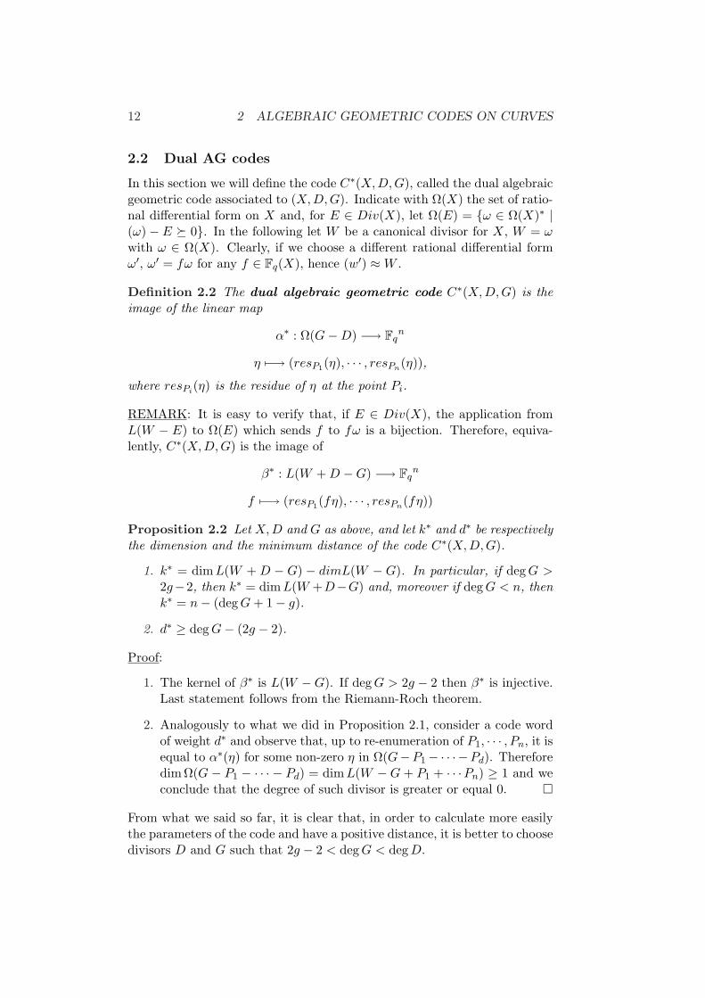
2.2 Dual AG codes

In this section we will define the code C∗(X,D, G), called the dual algebraicgeometric code associated to (X,D, G). Indicate with Ω(X) the set of ratio-nal differential form on X and, for E ∈ Div(X), let Ω(E) = ω ∈ Ω(X)∗ |(ω)− E º 0. In the following let W be a canonical divisor for X, W = ωwith ω ∈ Ω(X). Clearly, if we choose a different rational differential formω′, ω′ = fω for any f ∈ Fq(X), hence (w′) ≈ W .

Definition 2.2 The dual algebraic geometric code C∗(X, D, G) is theimage of the linear map

α∗ : Ω(G−D) −→ Fqn

η 7−→ (resP1(η), · · · , resPn(η)),

where resPi(η) is the residue of η at the point Pi.

REMARK: It is easy to verify that, if E ∈ Div(X), the application fromL(W − E) to Ω(E) which sends f to fω is a bijection. Therefore, equiva-lently, C∗(X, D, G) is the image of

β∗ : L(W + D −G) −→ Fqn

f 7−→ (resP1(fη), · · · , resPn(fη))

Proposition 2.2 Let X,D and G as above, and let k∗ and d∗ be respectivelythe dimension and the minimum distance of the code C∗(X,D, G).

1. k∗ = dimL(W + D − G) − dimL(W − G). In particular, if deg G >2g−2, then k∗ = dim L(W +D−G) and, moreover if deg G < n, thenk∗ = n− (deg G + 1− g).

2. d∗ ≥ deg G− (2g − 2).

Proof:

1. The kernel of β∗ is L(W −G). If deg G > 2g − 2 then β∗ is injective.Last statement follows from the Riemann-Roch theorem.

2. Analogously to what we did in Proposition 2.1, consider a code wordof weight d∗ and observe that, up to re-enumeration of P1, · · · , Pn, it isequal to α∗(η) for some non-zero η in Ω(G−P1− · · · −Pd). ThereforedimΩ(G− P1 − · · · − Pd) = dimL(W −G + P1 + · · ·Pn) ≥ 1 and weconclude that the degree of such divisor is greater or equal 0. ¤

From what we said so far, it is clear that, in order to calculate more easilythe parameters of the code and have a positive distance, it is better to choosedivisors D and G such that 2g − 2 < deg G < deg D.

2.2 Dual AG codes 13

Theorem 2.1 The codes C(X, D, G) and C∗(X, D, G) are dual to eachother.

Proof: First we show that C∗(X,D, G) ⊆ C(X, D,G)⊥. Let η ∈ Ω(G−D),f ∈ L(G). We have to show that α(f) α∗(η) = 0. But α(f) α∗(η) =∑n

i=1 f(Pi)resPi(η). Remark that the rational differential form fη belongsto Ω(−D), it can have simple poles just in the support of D. Hence∑

P∈X res(fη) =∑n

i=1 resPi(fη) =∑n

i=1 f(Pi)resPi(η). We conclude, bythe residues theorem, that α(f) α∗(η) = 0. Furthermore we know that

dimC(X,D, G)⊥ = n− k = n− dimL(G) + dimL(G−D) =

= dimL(W + D −G)− dimL(W −G) = k∗.

Thus C∗(X,D, G) = C(X, D,G)⊥. ¤

The following theorem shows that every dual algebraic geometric codes canbe obtained as algebraic geometric code and viceversa.

Lemma 2.1 There exists a differential form ω with simple poles with residues1 in the points of the support of D and such that C(X,D, W + D − G) =C∗(X, D, G), where W = (ω).

Proof: Chosen η ∈ Ω(X), let f ∈ Fq(X) be such that ordPif = −(ordPiη +1). The function fη has simple poles in P1, · · · , Pn. We can multiply fηwith a rational function to obtain residues equal to 1 in those simple poles.Let ω have such properties and let W = (ω). For every f ∈ L(W + D −G)we have resPi(fω) = f(Pi)resPi(ω) = f(Pi). Then α(f) = β∗(f) and so wefinally get C(X,D, W + D −G) = C∗(X, D, G). ¤

We saw in section 1 that two codes are called equivalent if they differ fora fixed permutation of the coordinates. We introduce a new equivalencerelation between codes such that it reflects, in some sense, the equivalencerelation between divisors. From now, when we will talk about equivalentcodes, we will mean equivalent according to the following definition.

Definition 2.3 Two codes C1 and C2, of length n over Fq, are called equiv-alent if there exists γ ∈ (F∗q)n such that γC1 = C2.

REMARK: It is clear that the dimension and the distribution of weightsof a code are not changed by the multiplication with a non zero elementγ ∈ (F∗q)n. We will study the properties of a code up to equivalence. It willbe useful also to decode a given encoded message.

Lemma 2.2 Let D =∑n

i=1 Pi be as above, G,G′ ∈ Div(X) whose supportsare disjoint sets from the ones of D and D′, G ≈ G′. Then C(X,D, G) isequivalent to C(X, D,G′) and C∗(X,D, G) is equivalent to C∗(X, D,G′).


Proof: Let (g) = G − G′ for g ∈ Fq(X). Since the supports of G andG′ are disjoint from supp(D), g(Pi) 6= 0, the multiplication with g is anisomorphism between L(G) and L(G′) and between Ω(G−D) and Ω(G′−D).Therefore C(X,D, G) = γC(X, D, G′) and C∗(X,D, G) = γC∗(X, D,G′),where γ = (g(P1), · · · , g(Pn)). ¤

Proposition 2.3 Let G ∈ Div(X) be such that 2G ≈ W + D. ThenC(X, D,G) is equivalent to its dual code.

Proof: It follows directly from Proposition 2.1 and Lemmas 2.1 and 2.2. ¤

REMARK: The viceversa in Proposition 2.3 does not hold. A counterex-ample can be found in [4, Remark 1 p. 894].

The next theorem gives an equivalent condition for the existence of G suchthat 2G ≈ W + D.

Theorem 2.2 (Weil) There exists G such that 2G ≈ W + D if and onlyif D is a square in Pic(X).

From what we saw previously it is quite natural to state the following lemma,which gives a sufficient condition to be self-dual.

Lemma 2.3 If there exists η ∈ Ω(X) with simple poles and residues equalto 1 in the poles of the support of D and such that 2G = K +D for K = (η),then C(X, D,G) is self-dual

Proof: Let ω and W be as in Lemma 2.1. We have η = fω for some nonzero rational function f . Thus K + D −G ≈ W + D −G and, by the proofof the previous lemma, C(X,D, K +D−G) = γC(X, D, W +D−G) whereγ = (f(P1), · · · , f(Pn)). But f(Pi) = resPiη/resPiω = 1, so C(X, D,G) =C(X, D,K +D−G) = C(X,D, W +D−G) = C∗(X,D, G) = C(X, D,G)⊥.¤

In general this condition is just a sufficient one. It is proved in [18, 3.12]that, if n > 2g + 2, then the condition is also a necessary one.

Let us now investigate the relations between the parameters of algebraicgeometric codes.

Lemma 2.4 Let 2g − 2 < deg G < n, d and d∗ the minimum distance ofC(X, D,G) and C∗(X, D,G) respectively. Then

1. n− deg G ≤ d ≤ n− deg G + g;

2. deg G− 2g + 2 ≤ d∗ ≤ deg G− g + 2.

2.3 Rational points on curves and lower bounds 15

Proof: The lower bounds are the ones proved in Lemmas 2.1 and 2.2, whilethe upper ones are the singleton bounds. ¤

Corollary 2.1 Let 2g−2 < deg G < n. If g = 0 then the codes C(X, D, G)and C∗(X, D,G) are MDS.

We saw some bounds for the distance of algebraic geometric codes. Wewould like now to see the distance as a geometric property of the divisorsD and G. Following what we did in the proof of Proposition 2.1, we remarkthat x ∈ C(X,D, G) has weight r > 0 if x = α(f), with f different from0 at r points among P1, · · · , Pn and vanishing at n − r points. Thusf ∈ L(G− Pi(r+1) − · · · −Pi(n)) for some i ∈ Sn. It follows that there existsa divisor D′ ¹ D of degree n− r such that L(G−D′) 6= 0. In our case wecan assume that α is injective, i.e. deg G < n. If there exists D′ ¹ D withdeg D′ = n−d then there exists a non zero word of weight ≤ d in C(X, D,G). So we have that the minimum distance of C(X, D, G) is the smallest integerd such that there exists a divisor D′ ¹ D with L(G−D′) 6= 0. Hence theminimum distance of a code can be obtained by looking at some subspacesof L(G).

Analogously, if deg G > 2g− 2, the minimum distance of C∗(X, D, G) isthe smallest integer d∗ such that there exists a divisor D′ ¹ D of degree dwith L(W +D′−G) 6= 0. We can state this sentence in the following way:x ∈ C∗(X, D,G) has weight r > 0 if x = β∗(f) for some f ∈ L(W + D−G)such that fω has non zero residue at r points among P1, · · · , Pn and zeroresidue in the remaining ones. Then fω is regular at n − r points and(fω) +

∑rj=1 Pi(j) + G = E, where E is an effective divisor with support

disjoint from Pi(1), · · · , Pi(r). So G −W ≈ −∑rj=1 Pi(j) + E. Viceversa,

if the last equality holds, then C∗(X,D, G) has a word of weight r. Thisallows us to state the following theorem.

Theorem 2.3 The minimum distance d∗ of C∗(X,D, G) is the smallestnumber of distinct points Pi(1), · · · , Pi(d∗) in the support of D such that, inPic(X), G −W =

∑d∗j=1 Pi(j) − E for any effective divisor E with support

disjoint from Pi(1), · · · , Pi(d∗).

Arguing this way we can compute the distribution of weights; in fact thenumber of code words with weight r is equal to (q − 1) times the numberof divisors D′ ¹ D of degree r linearly equivalent to a divisor of the formG−W + E for some E ∈ L(0), suppD′ ∩ suppE = ∅.

2.3 Rational points on curves and lower bounds

Let us deal again with the parameters of the algebraic geometric codes. Weknow that one of the central problems of coding theory is finding codes withrelative distance δ and rate R as large as possible. Let Vq be the set of pairs


(δ,R) coming from a linear code over Fq and Uq the set of limit points of Vq.Manin proved the following theorem, that gives us some information aboutUq.

Theorem 2.4 There exists a function α : [0, 1] → [0, 1] such that Uq =(δ,R) | 0 ≤ R ≤ α(δ). α is continuous in [0, q−1

q ], vanishes in [ q−1q , 0] and

is strictly decreasing.

Proof: see [17, th. 8 p. 2614]

REMARK: The function α above is exactly the same α we defined in section1. We already know, by the Gilbert bound, that 1−Hq(δ) ≤ α(δ).

For an algebraic geometric code C(X,D, G), we deduce by Proposition 2.1,if deg G < n, that

δ + R ≥ n− deg G

n+

deg G + 1− g + dimL(W −G)n

≥ 1 +1− g

n.

So we would like to find a family of codes with n going to infinity and g/nas small as possible asymptotically.

Lemma 2.5 Let Xi | i ∈ N be a sequence of smooth projective curvesover Fq, gi := g(Xi) and N1(Xi) the number of rational points (of degree 1)of Xi. If gi tends to infinity and limi→+∞ gi

N1(Xi)= γ, then the intersection

of the line δ + R = 1− γ with the square [0, 1]× [0, 1] is contained in Uq.

Proof: Let (δ,R) be a point of the line intersected with the square. Sinceγ is not negative, we have δ = 1 iff γ = 0 and it is clear that (1, 0) ∈Uq. We can restrict to δ < 1. Consider the codes Ci := C(Xi, Di, Gi),where Di is the sum of all the rational points P1, · · · , PN1(Xi) of Xi andGi := bN1(Xi)(1 − δ)cP1. The supports of Di and Gi are not disjoint, butthis is not a problem, as shown by the remark of page 11. Ri tends toR = R + l ≥ R, where l := limi→+∞

dim L(Wi−Gi)ni

. Let δ = limi→+∞ δi.

Now, we know that δi + Ri ≥ 1 + 1−gi+dim L(Gi−Wi)ni

, so δ + R ≥ 1 − γ + l.Therefore δ ≥ 1− γ − R + l = 1− γ −R = δ. Therefore the point (δ, R) isin Uq and R ≥ R, δ ≥ δ. By the previous theorem, (δ,R) ∈ Uq. ¤

NOTE: In the proof of [24][Part II, 5.2] the author discards l and saysthat Ri tends to 1− δ − γ = R. We are not sure this is true in general. Inany case, as we showed in the proof, it is sufficient to prove that Ri tendsto a value greater or equal R.

Corollary 2.2 Assuming the same hypotheses of the previous lemma, wehave α(δ) ≥ 1− δ − γ.


Let Nq(g) := max#X(Fq) | X is a smooth projective curve of genus g over Fq.It is clear by what we said above that we would like to know the value ofNq(g) and the function

A(q) := limg→+∞

Nq(g)g

.

To this end, we define the zeta function associated to a curve over Fq andlater on we will show how it is related to the number of rational points. Lets ∈ C, X a smooth projective curve over Fq.

ζ(X, s) :=∏p

(1−N(p)−s)−1,

where the product is over all the closed points of X and N(p) = qdeg p.Equivalently,

ζ(X, s) =∑

Dº0

N(D)−s,

where the sum runs over all the effective divisors of X and N(D) = qdeg D.Let δ be the g.c.d. of all the degrees of the effective divisors on X.

REMARK 1: The integer δ divides 2g − 2. In fact, by the Reimann-Rochtheorem, dimL(W ) > 0 and so there exists an effective divisor of degree2g − 2.

REMARK 2: If n > 2g − 2 and n = kδ, then there exists an effectivedivisor of degree n. Indeed we can write δ as a linear combination of degreesdi coming from effective divisors Di. δ =

∑mi=1 aidi where ai ∈ Z. Therefore

D := k∑m

i=1 aiDi has degree n. Recalling dimL(D) = deg D + 1 − g > 0and choosing f ∈ L(D) \ 0, we obtain that (f) + D is the wanted divisor.

For m ∈ Z, let Picm(X) = [D] ∈ Pic(X) | deg D = m. This is clearly agood definition, because principal divisors have degree 0. If there exists adivisor D′ of degree m, then #Picm(X) = #Pic0(X) := h via the bijection[D] 7→ [D]− [D′].

Lemma 2.6 The number an of effective divisors of degree n is equal to

∑

[D]∈Picn(X)

qdim L(D) − 1q − 1

.

Proof: If [D] ∈ Picn(X) then D + (f) is an effective divisor of degree n forevery f ∈ L(D) \ 0. Moreover [D] + (f) = [D′] + (f ′) implies [D] = [D′]and f/f ′ ∈ F∗q . ¤


We immediately deduce the following theorem from Riemann-Roch’s the-orem and what we observed previously:

Corollary 2.3 If n > 2g − 2 then an = h qn+1−g−1q−1 .

Changing variables, we can write ζ(X, s) = Z(X, q−s) = Z(X, t) for s, t ∈ C;so we have a power series that converges for |t| < 1. The zeta functionbecomes

ζ(X, s) =∑

n≥0

anq−sn =2g−2∑

n=0

antn ++∞∑

n=2g−1

antn,

where the index n in the second sum runs over the multiples of δ bigger than2g − 2. By REMARK 1 at page 17, if we put e = (2g − 2 + δ)/δ, eδ is thesmallest multiple of δ larger than 2g − 2. Hence we have

Z(X, t) =2g−2∑

n=0

antn ++∞∑n=e

anδtnδ =

polynomial +h

q − 1

+∞∑n=e

(qnδ+1−g − 1)tnδ

=h

q − 1(qg+1+δt2g−2+δ

1− (qt)δ− t2g−2+δ

1− tδ).

This way we obtained a rational function of t with poles at tδ = 1 and(qt)δ = 1.

The following theorems are the fundamental connection between the zetafunction and our problem.

Theorem 2.5

Z(X, t) =P1(t)

P0(t)P2(t)

where P0 = 1 − t, P2 = 1 − qt, P1 =∏g

i=1(1 − αit)(1 − αi) and αi arealgebraic integers of absolute value q

12 .

Proof: The proof in [2] uses only Riemann-Roch’s theorem, while the origi-nal one, due to Weil, needs intersection theory.

Let us indicate with Nr the number of points of degree one over Fqr

Theorem 2.6 (Hasse-Weil bound) |Nr − (1 + qr)| ≤ 2g√

qr.


A curve with exactly 1 + q + 2g√

q points over Fq is called maximal. Wesaid that an equivalent expression for ζ is

ζ(X, s) =∏p

(1−N(p)−s)−1 =∏

r≥1

(1− q−sr)−Nr

Expanding the log of the zeta function in its Taylor series, we have

log Z(X, t) =∑

r≥1

−Nr log(1− tr) =∑

r≥1

Nr

rtr

Hence, by Theorem 2.5,

log Z(X, t) = log P1(t)− log P0(t)− log P2(t) =

=g∑

i=1

(log(1− αit) + log(1− αit))− log(1− t)− log(1− qt) =

+∞∑

r=1

1 + qr −∑gi=1(αi + αi

r)r

tr

This means that the knowledge of the αi’s is enough to compute Nr for everyr. For r = 1 we have N1 = 1+q+a1 and |a1| = 2g

√q, so N1 ≤ 1+q+2g

√q.

We can now go back to the problem of finding the value (or at least somebounds) for A(q). It is clear that Nq(g) ≤ 1 + q + 2g

√q, so

A(q) = limg→∞

Nq(g)g

≤ 2√

q.

The first improvement of this bound is due to Ihara ([10, p. 721]).

Theorem 2.7 For every q we have A(q) ≤√

8q+1−12 .

Proof: Let bi = αi + αi ∈ R. We have

q + 1−g∑

i=1

bi = N1 ≤ N2 = q2 + 1−g∑

i=1

(α2i + αi

2) = q2 + 1 + 2gq −g∑

i=1

b2i

By the Cauchy’s inequality we get

g

g∑

i=1

b2i ≥ (

g∑

i=1

bi)2,

hence

N1 ≤ q2 + 1 + 2gq − g−1(g∑

i=1

bi)2 = q2 + 1 + 2gq − g−1(N1 − 1− q)2.


We get a quadratic equation on N1:

N21 − (2q + 2− g)N1 + (q + 1)2 − (q2 + 1)g − 2qg2 ≤ 0.

It turns out that

N1 ≤ 2q + 2− g +√

(8q + 1)g2 + (4q2 − 4q)g2

and so

A(q) ≤ limg→+∞

2q + 2− g +√

(8q + 1)g2 + (4q2 − 4q)g2g

=√

8q + 1− 12

.

¤

Arguing analogously, Drienfeld and Vladut ([26, th. 1]) proved that, forevery prime power q, we have A(q) ≤ √

q − 1. On the other hand, the fol-lowing theorem proves that we have an equality for the even powers of aprime number.

Theorem 2.8 (Tsfasman, Vladut, Zink) Let q = p2m be an even powerof the prime p. Then there is a sequence of curves Xi, defined over Fq havinggenus gi and Ni rational points, such that

limi→∞

Ni

gi=√

q − 1.

Proof: see [22, p. 28]

Using Lemma 2.5 we can state the following corollary:

Corollary 2.4 If q = p2m is an even power of a prime, then α(δ) ≥ 1− δ−(√

q − 1)−1.

It easy to check that the line R = 1 − δ − (√

q − 1)−1 intersects theGilbert curve R = 1−Hq(g) for q ≥ 43 and, since q has to be a square, wehave an improvement of Gilbert bound for q ≥ 49.

21

3 Decoding methods

A code is useful only if there exists an efficient way of decoding. Let usintroduce now two algorithms for decoding dual geometric codes. The firstone has been discovered by Skorobogatov and Vladut in 1990 and will becalled SV-algorithm for short. Nevertheless it is the easiest one and it isnot able to decode the full capability of the codes. Indeed we know that ifd is the minimum distance of a code, a good algorithm should be able tocorrect every error of weight at most t, where 2t < d. We will see that theSV-algorithm can surely correct errors of weight t if 2t < d− g, where g is,as usual, the genus of the curve X but it could not work for larger values oft. This is a non trivial restriction, since we saw that good codes are based oncurve with high genus. In order to solve this problem, Duursma improvedin 1992 the SV-algorithm and produced the more efficient processor we willdescribe later. The main idea of Duursma algorithm is to use a majorityvoting scheme. This technique has been used for the first time by Feng andRao to extend the first decoding algorithm for geometric codes, publishedby Justesen in 1989.

3.1 SV-algorithm

Let C∗(X, D, G) be a fixed dual geometric code based on a curve X of genusg, D = P1+, · · · , +Pn and 2g−2 < deg G. The designed distance of the codeis deg G− (2g− 2). Suppose we transmit a word c and the vector f = c + eis received.

Definition 3.1 For any vector f ∈ Fqn and any function ϕ in the function

field, the syndrome of f with respect to f is denoted by ϕ f and defined byϕ f =

∑ni=1 ϕi(Pi)fi. By convention we put ϕ f = ∞ if ϕ has a pole in

any Pi.

The dual of C∗(X, D,G) is the code C(X,D, G), so c belongs to C∗(X,D, G)if and only if x c = 0 ∀x ∈ C(X, D, G), hence if and only if ϕ c = 0∀ϕ ∈ L(G). It means that c is a word of the code if and only if, chosen abasis ϕ1, · · · , ϕu of L(G), the syndromes of c with respect to ϕi is 0 fori = 1, · · · , u. Moreover, for every ϕ ∈ L(G), ϕ e = ϕ f . What we try todo in the following is to deduce the error vector e from the syndromes of f .

Definition 3.2 An error location for e is a point Pi such that ei 6= 0. Anerror locator for e is a function Θ with no poles among P1, · · · , Pn andsuch that Θ(Pi) = 0 for every error location Pi.

Proposition 3.1 Let e have weight at most t and A be a divisor with nopoles among P1, · · · , Pn such that dimL(A) ≥ t + 1. Then an error locatorin L(A) exists.

22 3 DECODING METHODS

Proof: Let M be the support of e, i.e. the set of points Pi such that ei 6= 0.A function Θ is an error locator for e if and only if Θ(Pi) = 0 ∀Pi ∈ M . Letnow ϕ1, · · · , ϕs be a basis of L(A). A linear combination a1ϕ1 + · · ·+asϕs

is an error locator if and only if

a1ϕ1(Pi) + · · ·+ asϕs(Pi) = 0 ∀Pi ∈ M .

This is a system of at most t equations in s unknowns and, by hypothesis,s > t, so it has a non-trivial solution. ¤

The next proposition shows why finding an error locator is so important forour purpose.

Proposition 3.2 Let e be an error vector of weight at most t, A and Z twodivisors on X with support disjoint from P1, · · · , Pn, such that deg A ≤t + r and deg Z ≥ t + r + 2g − 1 for some r ≥ 0. If there exists an errorlocator Θ in L(A) then e is uniquely determined by Θ and the syndromes ofe with respect to the functions in L(Z).

Proof: Let M ′ be the set of points where Θ vanishes. Clearly M ′ containsM , the support of e. M ′ has at most t + r points. It is clear that ϕ e =∑

Pi∈M ′ ϕ(Pi)ei for every function without poles among P1, · · · , Pn. This istrue, in particular, for every function ϕ ∈ L(Z), so e is a solution of theequation

ϕ x =∑

Pi∈M ′ϕ(Pi)xi ∀ϕ ∈ L(Z).

If e′ is another solution, then ϕ (e−e′) = 0∀ϕ ∈ L(Z). It means that e−e′

belongs to C∗(X, D,Z). The minimum distance of this code is not less thant + r + 1 but if e and e′ have both support in M ′ then e− e′ has weight atmost t + r. Therefore e = e′. ¤

REMARK: We are trying to decode f , so we do not know e. In partic-ular, we do not know how to find an error locator for e and how to calculatethe syndromes. The second problem can be solved by choosing Z ¹ G. Inthis case the syndromes can be calculated from f instead of e. The solutionof the second problem is treated in the next proposition and it requires thethe introduction of a further auxiliary divisor.

Proposition 3.3 Let e have weight at most t and Y be a divisor with sup-port disjoint from the support of D such that deg Y ≥ t + 2g − 1. Then afunction Θ without poles among P1, · · · , Pn is an error locator for e if andonly if Θχ e = 0 for every χ ∈ L(Y ).

Proof: Let e′ = (Θ(P1)e1, · · · ,Θ(Pn)en). So we have Θχe =∑n

i=1 θ(Pi)χ(Pi)ei =χ e′. We will have that Θ is an error locator if and only if e′ = 0. So, if

3.1 SV-algorithm 23

Θ is an error locator then Θχ e = 0 for every function. Viceversa, supposeχ e′ = 0 for every χ ∈ L(Y ). It means that e′ ∈ C∗(X,D, Y ). Recallingthat deg Y ≥ t+2g−1, we get that the distance of this code is greater thant. This implies e′ = 0. ¤

Corollary 3.1 Let S = (ψiχj)i,j, where the elements ψi form a basis ofL(A) and the χ′js are a basis of L(Y ). Then Θ =

∑i aiψi is an error locator

for e in L(A) if and only if∑

i aiSi = 0, where Si is the ith row of S.

REMARK: Again, we want to calculate the syndromes of e from those off . If Y + A ¹ G then Θχ ∈ L(G) for every Θ ∈ L(A) and χ ∈ L(Y ), so thisis allowed.

Summarizing, we are looking for three auxiliary divisors A, Z and Y withthe required properties. Assume that deg G > 2g − 2.

Lemma 3.1 Suppose there exists a divisor A′ such that deg A′ ≤ deg G −(2g−1)−t and dimL(A′) ≥ t+1. Then there exist A, Z and Y with Z ¹ G,Y + A ¹ G and satisfying the hypotheses of the previous propositions.

Proof: If the support of A′ is disjoint from P1, · · · , Pn, set A = A′, oth-erwise add a suitable principal divisor. The first condition implies that, forsome u ≥ 0, t + 1 + u = dimL(A) ≥ deg A + 1 − g, so deg A ≤ t + u + gand deg A = t + r for some r ≥ 0. We can now put Z = G and Y = G−A.We get deg Z = deg G ≥ A + (2g − 1) + t ≥ r + t + 2g − 1 and deg Y ≥deg G− deg G + 2g − 1 + t = t + 2g + 1. ¤

The conditions of Lemma 3.1 guarantees that 2t < d, so the code can correcterrors of weight t. We wondering when there exists a divisor A′ such thatdeg A′ ≤ deg G−(2g−1)− t and dimL(A′) ≥ t+1. We give now a sufficientcondition.

Lemma 3.2 If 2t < deg G − (3g − 2), then A′ with the required propertiesexists.

Proof: By the hypothesis, t + g ≤ deg G− 2g + 1− t, so there exists a, witht + g ≤ a ≤ deg G− 2g + 1− t. Set A′ = aQ, where Q is a point not in thesupport of D. dim L(A′) ≥ t + g + 1− g = t + 1. ¤

It is clear now what our strategy to decode a message is. Let us writeformally the SV-algorithm.

SV-ALGORITHM: Let c be a word of the code C∗(X,D, G) defined over a


curve of genus g, with deg G > 2g − 2. Let f = c + e, where e is the errorvector.

STEP 0: Preliminary stepThis step is performed only once for any code. Choose a divisor A such thatdimL(A) > t and deg A ≤ deg G− (2g − 1)− t. Choose divisors Z, Y suchthat Z ¹ G,Y + A ¹ G, deg Z ≥ deg A + 2g − 1 and deg Y ≥ t + 2g − 1.Choose bases ϕ1, · · · , ϕu of L(Z), ψ1, · · · , ψs of L(A) and χ1, · · · , χrof L(Y ).

STEP 1: Syndrome calculationCalculate the matrix S = (ψiχj f)i,j .

STEP 2: Error locatorFind α1, · · · , αs such that α1S

1 + · · ·+ αsSs = 0, where Si is the ith row of

S. Θ =∑s

i=1 αiψi is an error locator for e in L(A).

STEP 3: Error locationsLet M ′ be the set of points where Θ vanishes. This set contains the errorlocations.

STEP 4: Error values calculationSolve the system of equations

∑

Pl∈M ′ϕi(Pl)el = ϕi f for i = 1, · · · , u.

Extend the solution by putting ej = 0 if Pj 6∈ M ′. (e1, · · · , en) is the errorvector.

3.2 A cubic curve

Before introducing the Duursma algorithm, we will give an example of geo-metric code and we will use the SV-algorithm to correct en error of weight2 produced during the transmission of a word. The curve X is given by theequation x3 + y3 + z3 = 0.

• Points over F2

P0 = (0 : 1 : 1) P1 = (1 : 1 : 0) P2 = (1 : 0 : 1)

• Points over F4=F2[z]

(x2+x+1)= F2[α]

3.2 A cubic curve 25

points over F2

P3 = (α : 1 : 0) P4 = (α + 1 : 1 : 0) P5 = (α : 0 : 1)P6 = (α + 1 : 0 : 1) P7 = (0 : α : 1) P8 = (0 : α + 1 : 1)

• Points over F8=F2[x]

(x3+x2+1)= F2[ω]

points over F2

Q1 = (ω : ω2 + 1 : 1) Q2 = (ω2 : ω2 + 1 : 1)Q3 = (ω2 + ω + 1 : ω + 1 : 1) Q4 = (ω2 + 1 : ω : 1)Q5 = (ω2 + ω : ω2 : 1) Q6 = (ω + 1 : ω2 + ω + 1 : 1)

First of all, the curve is smooth if char (Fq) 6= 3, as the system

x3 + y3 + z3 = 03x2 = 03y2 = 03z2 = 0

has no solutions in P2. Therefore the genus can be calculated by Pluckerformula and it is equal to 1. We want to check that we did not forgetany point of X. Recalling that the genus is 1, it is sufficient to calculatethe number of points over F2. We get N1 = 3, q = 2, g = 2, so 3 =2 + 1− (α1 + α1). Hence α1 = −α1 and, recalling that |α1| =

√2, we have

α1 = i√

2. So we can now compute the number of points over F2r :

N2 = 22 + 1− (−2− 2) = 9

N3 = 23 + 1− (−i√

2 + i√

2) = 9

N4 = 24 + 1− 8 = 9.

So the points over F16 are those over F4. In general we have

Nr =

qr + 1, if r oddq2k + 1 + (−1)k+12k+1 if r = 2k.

Let us consider now the code C∗(X, D, G) where D = P1 + · · · + P8 andG = aP0 with 1 ≤ a ≤ 7. The length is 8, the dimension 8 − a and theminimum distance is at least a. For example, if a = 6, C∗(X, D, G) is a[8, 2,≥ 6]-code, while C(X, D,G) is a [8, 6,≥ 2]-code. Now we know thatC∗(X, D, aP0) is able to correct errors up to t, if 2t < d ≤ a. To correctan error of weight 2, a = 5 should be sufficient. But in the SV-algorithmwe need a divisor A of degree at most a − 3 such that dimL(A) > 2. ButdimL(A) = deg A so this is impossible for a = 5. For codes defined overthis cubic curve, Lemma 3.2 gives a necessary condition. So we have to takea = 6. Let us find a basis of L(aP0). P0 is in the affine plane z = 1, so we can


use affine coordinates and, around P0, the curve is given by x3 + y3 +1 = 0.The tangent line in P0 is y + 1 = 0, so vP0(x) = 1 while vP0(y + 1) = 3(P0 is an inflexion point). Consider the functions xiyj(y + 1)−(i+j). Theyhave a pole of order 3j + 2i in P0. We can easily see that the functionsfij := xiyj(y+z)−(i+j) have no other poles on X, so (fij) = −(3j+2i)P0+Ewith E effective divisor. We obtain that fij ∈ L(G) if 0 ≤ 3j + 2i ≤ a.By choosing suitable i and j, we find a linearly independent functions inL(aG), i.e. a basis of L(aP0). For instance, if a = 6, the functions 1,

xy+z , y

y+z , x2

(y+z)2, xy

(y+z)2and x3

(y+z)3form a bases of L(6P0) and they have

poles of order respectively 0, 2, 3, 4, 5 and 6. Therefore, evaluating thefunctions in P1, · · · , P8, a generator matrix for C(X,D, 6P0) (a check matrixfor C∗(X,D, 6P0)) is

H =

1 1 1 1 1 1 1 11 1 α α + 1 α α + 1 0 01 0 1 1 0 0 α + 1 α1 1 α + 1 α α + 1 α 0 01 0 α α + 1 0 0 0 01 1 1 1 1 1 0 0.

.

It can be proved that there are 6 linearly independent columns, so the min-imum distance is exactly 6. Let us try to decode the vector f = c + ewhere

c =(

α α α + 1 1 α + 1 1 0 0)

e =(

α 0 1 0 0 0 0 0)

f =(

α α α + 1 1 α + 1 1 0 0).

When the support of G is of the form bQ for some point G, the mostnatural choice for A is a divisor of the form cQ, so we can take as ba-sis of L(A) a subset of the special basis of L(G). In our example we setA = 3P0,Z = 4P0, Y = 3P0. A basis of L(A) and L(Y ) is 1, x

y+z , yy+z,

while 1, xy+z , y

y+z , x2

(y+z)2 is a basis of L(Z). The matrix of the syndromes

is

S =

1 f xy+z f y

y+z fx

y+z f x2

(y+z)2 f xy

(y+z)2 f

yy+z f xy

(y+z)2 f y2

(y+z)2 f

=

α + 1 0 α + 10 1 0

α + 1 0 α + 1

.

The error locator Θ in L(A) is given by Θ = λ1 + λ2x

y+z + λ3y

y+z where

λ1

α + 10

α + 1

+ λ2

010

+ λ3

α + 10

α + 1

=

000

.

3.3 The Duursma algorithm 27

For example we can take λ1 = λ3 = 1, λ2 = 0, Θ = 1 + yy+z . Θ vanishes in

P1, P3 and P4, hence we have to find the unique solution of

1 1 11 α α + 11 1 11 α + 1 α

e1

e3

e4

=

α + 10

α + 11

.

The unique solution is e1 = α, e3 = 1, e4 = 0. We conclude that

e =(

α 0 1 0 0 0 0 0).

3.3 The Duursma algorithm

In the SV-algorithm we looked for an error locator Θ in L(A) and, in order tofind it, we needed another auxiliary divisor Y . The syndromes for productsbetween functions in L(A) and L(Y ) could be calculated from the receivedvector if Y +A ¹ G. But from this condition we get the restriction deg G ≥3g + 2t− 1. We will describe soon how this restriction can be overtaken bythe so-called majority voting method. Roughly speaking, it allows to deducefurther syndromes of e from the known ones, calculated from f .Let C∗(X,D, G) be as usual. This code can correct errors of weight up to t,where 2t ≤ deg G−2g +1. Take a point Q which is not in the support of D.Put G′ = G − (deg G − 2g + 1)Q. G′ ¹ G, so C∗(X,D, G) ⊆ C∗(X,D, G′)and deg G′ = 2g + 2t − 1. Choose a divisor A with deg A = t and supportdisjoint from that of D. Define A′ = G′ − A − (2g − 1)Q. Also deg A′ = t.Our strategy is to find an error locator in the space L(A+rQ) or L(A′+rQ)with r ≤ 2g− 1 and r as small as possible. For sure it can be done since, byProposition 3.1, there exists an error locator in L(A+gQ), as deg(A+gQ) =t + g and dimL(A + gQ) ≥ t + 1. Moreover, Proposition 3.3 tells we cancalculate it by using the syndromes for products of functions in L(A + gQ)and L(A′ + (2g − 1)Q).

Definition 3.3 Let Q be a rational point of the curve X. For any divisorsH and any non-zero function Θ, the H-order of Θ with respect to Q is thesmallest integer m such that Θ belongs to L(H + (m− deg H)Q), if such aninteger exists. Otherwise the H-order is defined to be +∞. The H-order ofΘ with respect to Q is denoted by µH,Q(Θ) (or simply µH(Θ) when Q doesnot change).

Proposition 3.4 Let Q be a fixed rational point. The following propertieshold for divisors H, H ′ and non-zero functions Θ, Θ′:

1. Let µH(Θ) = r < ∞. Then r ≥ 0 and vQ(Θ) = d(H) − H(Q) − r,where H(Q) is the coefficient of Q in H.


2. Let H < K and µH(Θ) = r < ∞. Then µK(Θ) = r + deg(K −H) −(K −H)Q, where (K −H)Q is the coefficient of Q in K −H.

3. If µH(Θ) = r < ∞ and µH′(Θ′) = r′ < ∞, then µH+H′(ΘΘ′) = r + r′.

Proof:

1. By contradiction we assume r < 0. Then Θ ∈ L(H + (r − deg H)Q).But deg(H + (r − deg H)Q) = r < 0 and so L(H + (r − deg H)Q) =0. Therefore Θ = 0, which is a contradiction because Θ 6= 0 byhypothesis. By definition of H-order, Θ belongs to L(H+(r−deg H)Q)but it is not in L(H + (r − deg H)Q). It means that (Θ) + H +(r − deg H)Q º 0 but (Θ) + H + (r − 1 − deg H)Q 6º 0. HencevQ(Θ)+H(Q)+ r−deg H ≥ 0 but vQ(Θ)+H(Q)+ r−1−deg H < 0.We finally have that µK(Θ) = r + deg(K −H)− (K −H)Q.

2. If Θ ∈ L(H + kQ) then Θ ∈ L(K + kQ), so µK(Θ) < ∞. By part (1),we obtain µK(Θ) = deg K −K(Q)− vQ(Θ) = deg(K −H) + deg H −(K −H)Q−H(Q)− vQ(Θ) = r + deg(K −H)− (K −H)Q.

3. By definition of order, Θ ∈ L(H + (r − deg H)Q) and Θ′ ∈ L(H ′ +(r′−deg H ′)Q). Since (ΘΘ′) = (Θ)+(Θ′), we have ΘΘ′ ∈ L(H +H +(r + r′ − deg H − deg H ′)Q) = r + r′. Hence µH+H′(ΘΘ′) < +∞ andso we can apply point (1). Recalling that vQ(ΘΘ′) = vQ(Θ) + vQ(Θ′),we obtain µH+H′(ΘΘ′). ¤

Corollary 3.2 Let ψ1, · · · , ψm be functions such that µH(ψ1) < · · · < µH(ψm)is a complete list of the possible values µH(ψ) ≤ deg H+r. Then ψ1, · · · , ψmis a basis of L(H + rQ).

The main object involved in the Duursma algorithm is the syndromes tableS. As in the SV-algorithm, suppose a word c is transmitted and f = c + eis received, where e is an error vector of weight not bigger than t. Usingthe previous corollary, we can choose bases φk of L(A + A′ + (3g− 1)Q), ψi

of L(A + (2g − 1)Q) and χj of L(A′ + (2g − 1)Q), where µA+A′(φk) = k,µA(ψi) = i and µA′(χj) = j. We use the A-order to index the rows and theA′ for the columns. We call these indices the orders of the rows and thecolumns. S is defined by

Sij = ψiχj e

and so S is a (t + g) × (t + g) matrix. By Proposition 3.4, the (A + A′)-order of the (i, j)-entry is i + j. The knowledge of S is sufficient to find anerror locator. In fact by Corollaries 3.2 and 3.1, knowing the rows 1, · · · , imeans knowing all the syndromes ψχ, where ψ ∈ L(A + (i − t)Q), χ ∈L(A′+(2g−1)Q). If there exists ψ such that ψχ e = 0 for every χ, then ψis an error locator in L(A + (i− t)Q). Thus we can check if an error locator


in L(A + (i− t)Q) exists. Analogously for columns up to order j to find anerror locator in L(A′ + (j − t)Q). The fundamental problem is that we donot know e, but we have just f , so we cannot calculate all the syndromes inS.

Nevertheless, observe that φiχj belongs to L(A + A′ + (i + j − 2t)Q) =L(G + (i − j − deg G)Q), so if i + j deg G, then G + (i + j − deg G)Q ¹ Gand ψiχj e = ψiχj f , hence the entries of order up to deg G are known.

Let us say that a row (or column) is known if all the entries in that row(or column) are known, unknown otherwise. By construction, the ordersof rows and columns are less or equal 2g − 1 + t, so the rows and columnsof order at most t are known, as, for their (i, j)-entries, we have i + j ≤t + 2g − 1 + t = 2g − 2t− 1 ≤ deg G.

There exists in every row an element with A′-order equal to 2g − 1 + t,so, if i > t + deg G− (2g + 2t− 1), the row is initially unknown. The orderof the t-th row is at most t + g − 1.

If deg G ≥ 3g + 2t − 1 then for the (i, j)-entries in the first t rows, wehave i + j ≤ t + g − 1 + 2g − 1 + t = 2t + 3g − 2 < deg G, so the first trows are known. In this case these rows form the syndrome table used bythe SV processor with auxiliary divisors A + rQ and A′ + (2g − 1)Q, wherer + t is the order of the t-th row. The first t rows can be known even ifdeg G < 3g + 2t− 1.

It can happen that, from the known rows and columns, we cannot findany error locator. This case is more interesting because we have to use atechnique called majority voting in order to deduce more syndromes fromthe known entries. As a preliminary remark, the next lemma shows how,from a new entry, we can obtain many others.

Lemma 3.3 Suppose all the syndromes φ e are known, for µA+A′(φ) < s,and an entry of order s is known. Then all the entries of order s are known.

Proof: Let Sij be the known entry of order s. It means that i + j = s andSij = ψiχj e. ψiχj ∈ L(A+A′+(s−2t)Q), so it can be written as aφs +φ′,where a ∈ Fq, µA+A′(φ′) < s. Sij = aφs e + φ′ e and φ′ e is known byhypothesis, hence we can calculated φs e. By linearity we can deduce thesyndromes of the functions in L(A + A′ + (s − 2t)Q), hence every entry oforder s. ¤

Motivated by the proof of the lemma, it is convenient to write every productψiχj with i + j > deg G as a linear combination of the φi’s. Moreover, wecan stop when i+ j > 3g−1+2t, because, in the worst case, we will find anerror locator in L(A + gQ), so we will work with function of (A + A′)-orderat most 3g − 1 + 2t.

We recall that our aim is to find an error locator Θ with µA(Θ) = uor µA′(Θ) = u and we want u as small as possible, since finding an error


locator with µA(Θ) requires the knowledge of the rows with order up to u.The following proposition describes how the increasing rate of the numberof error locators depends on u.

Proposition 3.5 Let e have weight at most t = deg A = deg A′ and lett ≤ u ≤ g+t. Suppose there are no error locators Θ for e with µA(Θ) < u orµA′(Θ) < u. For r between u and 2g−1+t, let r′ be the value 2g−1+t+u−r.Let p be the number of r between u and 2g1 + t such that there are errorlocators Θ, η for e with µA(θ) = r and µA′(η) = r′, and let q be the numberof r between u and 2g − 1 + t such that there is neither an error locator Θwith µA(θ) = r nor an error locator η with µA′(η) = r′. Then p− q ≥ u− t.

Proof: First remark that, for r running in the interval [u, 2g− 1 + t], also r′

does the same, and their sum is constantly equal to 2g − 1 + t + u. Define

J = r | u ≤ y ≤ 2g − 1 + t,

I = r ∈ J | there exists an error locator with A-orderr,I ′ = r ∈ J | there exists an error locator with A′-order r′.

We getp = #(I ∩ I ′)

q = #(J \ (I ∪ I ′)) = 2g + t− u−#(I ∪ I ′).

We claim that both #I and #I ′ are greater or equal t.Put De =

∑ei 6=0 Pi, i.e. the sum of the error locations. An error locator

in L(A+(r−t)Q) is an element of L(A+(r−t)Q−Be). Consider r = 2g−1+t.We have to study L(A+(2g−1)Q−Be). We have deg(A+(2g−1)Q−Be) ≥2g− 1, so dimL(A+(2g− 1)Q−Be) ≥ g. By Corollary 3.2 we can choose abasis of L(A + (2g − 1)Q−Be) by choosing ρi with different µA−Be(ρi) = iand µA−Be(ρi) ≤ 2g − 1 + t − deg Be. Recalling that µA(ρi) ≥ u becausethere are no error locators with A-order less than u, we get, by Proposition3.4(b), µA−Be(ρi) = i + deg Be ≤ 2g1 + t. We found at least g error locatorswith different orders between u and 2g − 1 + t. Thus #I ≥ g.

Arguing analogously on the columns, we get #I ′ ≥ g. ¤

A fundamental role in the algorithm we are explaining is played by row andcolumn candidates. We know that, in order to find an error locator with A-order r, we test a function ψ with all the functions in L(A′+(2g− 1+ t)Q).More explicitly, if Si is the i-th row of S, we look for

∑i≤r aiψi, where∑

i≤r Si = 0. But many times we know just the syndromes for the productswith function of A′-order up to r′, so we can test ψ just with functions inL(A′ + (r′ + t)Q). If r′ < 2g− 1 + t we are not sure ψ is an error locator. Itis just a possible candidate. This motivates the formal definition below.


Definition 3.4 A function θ is called a row candidate of order (r, r′) ifµA(Θ) = r and Θη e = 0 for all the functions η with µA′(η) ≤ r′. We sayΘ to be normalized if Θ = ψr + Θ′, with µA(Θ′) < r.

A function θ is called a column candidate of order (r, r′) if µA′(η) = rand Θη e = 0 for all the functions Θ with µA(Θ) ≤ r. η is normalized ifη = χr′ + η′, with µA′(η′) < r′.

REMARKS: We said above that a row candidate of order (r, 2g − 1 + t) isan error locator. Clearly a row candidate of order (r, r′) is, a fortiori, a rowcandidate of order (r, r′′) for every r′′ < r′. Similarly for column candidates.

The following proposition shows how to find candidates, and their rela-tions with the syndromes matrix. We will state it just for row candidates.Corresponding properties hold for column candidates.

Proposition 3.6 1. Let S|rr′ be the matrix (Sij)i≤r,j≤r′. A function∑i≤r aiψi with ai 6= 0 is a row candidate of order (r, r′) if and only if∑i≤r Si = 0, where Si is the i-th row of S|rr′.

2. If Θ is a normalized row candidate of order (r, r′ − 1) and η is anormalized column candidate of order (r − 1, R′), then

Θχr′ e = ψrη e.

3. If θ1 and Θ2 are distinct normalized row candidates of order (r, r′− 1)and Θ1χr′ e 6= Θ2χr′ e, then there are no column candidates of order(r − 1, r′).

Proof:

1. It follows directly from Corollary 3.2 and the linearity of the syndromewith respect to the functions.

2. Write Θ = ψr + Θ′ with µA(Θ′) < r, η = χr′ + η′ with µA′(η′) < r′.We get Θχr′ e = Θη e−Θη′ e = Θη e = ψrη e+Θ′η e = ψrη e.

3. By contradiction, assume there exists a column candidate of order(r − 1, r′). Then, by (2), Θ1χr′ e = ψrη e = Θ2χr e, which is acontradiction. ¤

We are now ready to learn how to add new syndromes in the matrix S.Suppose all the syndromes ϕ e are known for µA+A′(ϕ) < s, but ϕs e isunknown. This implies that all the entries of order less than s are known,


but no one of order s. In this case s ≥ deg G + 1 ≥ 2t + 2g. Supposemoreover that the known rows and column did not give any error locator.We consider now all the entries Srr′ where r + r′ = s. Since all the entriesin S|r,r′−1 and S|r−1,r′ are known, we are able to decide whether there area row candidate Θ of order (r, r′ − 1) and a column candidate η of order(r − 1, r′). If both exist, we can choose them normalized and we shall callSrr′ a test entry for s. Note that the value Θχr′ e is independent by thethe chosen row candidate.

If there exists an error locator with A-order r, we can guess it is exactlyΘ. In this case Θ e = 0. But θ = ψr + Θ′, so 0 = Θχr′ e = ψrχr′ e + Θ′χr′ e. Thus ψrχr′ e = −Θ′χr′ e, where the right hand side isknown, as µA+A′(−Θ′χr′) < s. The proof of Lemma 3.3 shows how it ispossible to deduce from ψrχr′ e the value of ϕs e. Let us call this valuethe vote of the entry Srr′ . As consequence of the previous proposition,observe that the same vote for Srr′ could be obtained by supposing η to bean error locator.

We are not sure this vote is the true value of ϕs e, since it comes fromthe guess Θ e = 0. Nevertheless, the next proposition ensures that themajority of votes are correct.

Proposition 3.7 The number of test entries Srr′ with r + r′ = s producingcorrect votes exceeds those producing incorrect votes by at least s−2g−2t+1 > 0. In particular there is at least one of such a test entry.

Proof: Let u = s−2g− t+1. As s ≥ 2g+2t, u ≥ t+1 and we are allowed toapply Proposition 3.5. If r′ is defined as in there, the pairs (r, r′) are exactlythose such that r + r′ = s. We claim that the number of correct votes is atleast p and the number of incorrect votes is at most q.

Suppose there exist error locators Θ, η with µA(Θ) = r and µA′(η) = r′.We can suppose them normalized. Θ is also a row candidate of order (r, r′−1)and η is a column candidate of order (r− 1, r′), so, for each normalized rowcandidate Θ1 of order (r, r′ − 1), Θ1χ − r′ e = Θχ − r′ e = 0. It meansthe vote of Srr′ was correct.

On the other hand, suppose Srr′ gives an incorrect vote, i.e. there exista normalize row candidate Θ1 of order (r, r′ − 1), a column candidate η1 oforder (r − 1, r′) and Θ1χr′ e 6= 0. Suppose by contradiction there existsan error locator θ with µA(θ) = r. Then 0 = Θχr′ e = Θ1χr′ e 6= 0.For similar reasons it is impossible there exist an error locator with A′-orderequal to r′.

We finally obtain that the difference between correct and incorrect votesis at least p− q ≥ u− t = s− 2g − 2t + 1. ¤

REMARK: The existence of a basis element ϕs for s ≥ 2t + 2g implies thatthere is an entry of order s in S. Indeed ϕs can be chosen as a product ψrχr′ .


Let us write now the Duursma algorithm.

DUURSMA ALGORITHM: Let c be a word of the code C∗(X, D, G), basedon a curve X of genus g and let f = c + e be the received word, wherewt(e) ≤ t and deg G ≥ 2t + 2g − 1.

STEP 0: Preliminary stepThis step is done just once for every fixed code. Choose a divisor A withdeg A = t and support disjoint from the one of D. Pick a rational pointQ not in the support of D. Put G′ = G − (deg G + 2g + 2t − 1)Q andA′ = G′ − A − (2g − 1)Q. Choose bases ϕ0, · · · , ϕ3g+2t−1 of L(A + A′ +(3g− 1)Q), ψ0, · · · , ψ2g+t−1 of L(A + (3g− 1)Q) and χ0, · · · , χ2g+t−1 ofL(A′ + (2g − 1)Q), indexed respectively by the (A + A′), A and A′ orders.For all indexes i, j with deg G < i + j ≤ 3g + 2t − 1 write ψiχj as a linearcombination of ϕ0, · · · , ϕi+j .

STEP 1: Syndrome calculationConstruct the syndromes table S in the following way: S is a (t+g)×(t+g)matrix where rows and columns are indexed by A-orders and A′-orders. Fori + j ≤ deg G, Sij = ψiχj f . If all the syndromes are 0, then f belongs toC∗(X, D, G). Leave the cells of order greater than deg G blank. Calculatethe syndromes ϕs f for s ≤ deg G.

STEP 2: Test for error locatorLet u be the maximal order of the known rows. Look for a non-zero solutionof the linear system

∑

i≤u

αiSi = 0

where Si is the i-th row of S. If a solution α exists, then∑

i≤u αiψi is anerror locator: go to step 5.Let u be the maximal order of the known columns. Look for a non-zerosolution of the linear system

∑

j≤u

βjSj = 0

where Sj is the j-th column of S. If a solution β exists, then∑

j≤u βjχj isan error locator: go to step 5.

STEP 3: Estimate additional syndromesAssume that every entry of order s−1 is known, while no entry of order s is


known. For each pair (r, r′) with r + r′ = s, try to solve the linear systems

∑

i<r

Sikαi = −Srk for k < r′

∑

j<r′Skjβj = −Skr′ for k < r.

If both solutions α and β exist, put Srr′ = −∑i<r αiSir′ = −∑

j<r′ βjSrj .and call Srr′ a test entry for s.

STEP 4: Majority votingFor each test entry Srr′ use the expressions of ψrχr′ in terms of the basis ϕi,and the known syndromes φi e for i < s, to calculate the vote ϕs e. Thetrue value ϕs e is the vote that occurs most frequently. Using this value,recalculate all the syndromes ψrχr′ (all but the test entries that gave correctvotes). If an additional column or row is known, go to step 2, otherwise goto step 3.

STEP 5: Find error locationsWe found an error locator Θ with µA(Θ) ≤ t + g or µA′(Θ) ≤ t + g. Deter-mine the set M = Pi ∈ supp(D) | Θ(Pi) = 0. This set contains the errorlocations.

STEP 6: Calculation of error valuesSuppose we found an error locator using rows (or columns) up to order u.Then the syndromes ϕk e for k ≤ u + 2g + t − 1 are known. Solve theequations

∑

Pl∈M

ϕk(Pl)el = ϕk e for k ≤ u + 2g + t− 1.

Extend the unique solution (el : Pl ∈ M) of this set of equations by puttingel = 0 for Pl 6∈ M . Then e = (e1, · · · , en) is the error vector.

REMARK: The uniqueness of the solution in step 6 follows from Theorem3.1 with divisors A + (u− t)Q and A + A′ + (u + 2g + t− 1− 2t)Q.

3.4 Example

Let us go back to the code C∗(X, D,G), where X is the curve x3+y3+z3 = 0,P0 = (0 : 1 : 1), G is the sum of the other point over F4 and D = aP0. Insubsection 3.2 we said that the SV-algorithm requires a ≥ 6 to correct anerror of weight 2. We shall take a = 5 and use the Duursma algorithm.

3.4 Example 35

Suppose we received f = x + e, where

x = ( α α + 1 1 0 0 0 1 0 )

e = ( α 0 0 1 0 0 0 0 )

f = ( 0 α + 1 1 1 0 0 1 0 ).

We chose a word x in C∗(X, D, 5P0) but not in C∗(X, D, 6P0). The naturalchoices in the preliminary step are Q = P0 and A = 2P0, so all the bases canbe chosen as subsets of the single basis of L(6P0) = L(A + A′ + (2g− 1)P0).We get A′ = A = 2P0 and bases

ϕ0 = 1, ϕ2 =x

y + z, ϕ3 =

y

y + z, ϕ4 =

x2

(y + z)2, ϕ5 =

xy

(y + z)2, ϕ6 =

x3

(y + z)3,

ψ0 = ϕ0, ψ2 = ϕ2, ψ3 = ϕ3,χ0 = ϕ0, χ2 = ϕ2, χ3 = ϕ3

In the syndromes table S we know all the entries of order at most 5. JustS33 is unknown. Write ψeχ3 = ϕ6. The syndromes table is

S =

α + 1 1 α + 11 0 1

α + 1 1

.

Observe that S is symmetric, so working with rows or columns gives thesame final result. The system

α1

α + 11

α + 1

+ α2

101

=

000

has just a trivial solution, so there are not locators with A-order 2. Theonly entry of order 6 is S33, so it must be a test entry by Proposition 3.7,i.e. there must be a row candidate of order (3, 2). Indeed a solution for

α0

(α + 1

1

)+ α2

(10

)=

(α + 1

1

)

is given by α0 = 1,α2 = 0, so S33 = S03 = α + 1. This is the only vote,hence it must be correct. The syndromes matrix is now

S =

α + 1 1 α + 11 0 1

α + 1 1 α + 1

.


A new row has been found and the matrix is totally known, so there must bean error locator. We now remark that α0 = 1 = α3, α2 = 0 is a solutionfor the system

α0

α + 11

α + 1

+ α2

101

+ α3

α + 11

α + 1

=

000

hence Θ = ψ0 + ψ3 = 1 + yy+z is an error locator for e. It vanishes in P1, P3

and P4. We have to solve the system

ϕk(P1)e1 + ϕk(P3)e3 + ϕk(P4)e4 = ϕk e for k ≤ 6.

It is easy to see that e1 = α, e3 = 0, e4 = 1 is the only solution for

1 1 11 α α + 11 1 11 α + 1 α1 α α + 11 1 1

e1

e3

e4

=

α + 11

α + 101

α + 1

.

Therefore we obtain

e =(

α 0 0 1 0 0 0 0)

3.5 Another example: the Klein quartic

The previous example does not show explicitly the majority voting mech-anism. To emphasize it, we have to consider an example such that thesyndromes matrix contains a larger number of unknown entries.

The curve X defined by x3y + y3z + xz3 = 0 is called the Klein quartic.X, over a field with characteristic different from 7, is smooth, so its genuscan be easily calculated by the Plucker formula and it equals 3. We shalloften work with F2 and its algebraic extensions. The point of the Kleinquartic over F2 are:

P0 = (0 : 0 : 1) P1 = (0 : 1 : 0) P2 = (1 : 0 : 0).

Let F16 the field of 16 elements, based on the irreducible polynomial x4 +x3 + 1. For short, every element y of this field will be denoted by an integern between 0 and 15, such that, if (a3, a2, a1, a0)2 is the binary representationof n, then y = a3x

3 + a2x2 + a1x + a0 in F2[x]/(x4 + x3 + 1).

3.5 Another example: the Klein quartic 37

The points of the Klein quartic over F16 are those over F2 and

P3 = (10 : 11 : 1) P4 = (11 : 10 : 1)

P5 = (3 : 10 : 1) P6 = (5 : 11 : 1) P7 = (8 : 10 : 1) P8 = (15 : 11 : 1)

P9 = (10 : 2 : 1) P10 = (11 : 4 : 1) P11 = (10 : 9 : 1) P12 = (11 : 14 : 1)

P13 = (6 : 8 : 1) P14 = (13 : 15 : 1) P15 = (7 : 3 : 1) P16 = (12 : 5 : 1).

The points in the same row are conjugate. P3 and P4 are over F4 (they arerational points of degree 2 over F2).

Consider the codes C∗(X, D, aP0), where D = P1+ · · ·+P16 and 5 ≤ a ≤ 15.They have dimension 18− a and minimum distance greater or equal a− 4.In this example we want to correct errors of weight at most 3, so we needa ≥ 11.

The function z/x has a pole of order 3 in P0, while y/z has a zero ofmultiplicity 1 in P0. In the following table the functions forming a base forL(16P0) and their pole orders in P0.

pole ord. 0 3 5 6 7 8 9 10 11 12 13 14 15 16function 1 z

xyzx2

z2

x2y2zx3

yz2

x3z3

x3y2z2

x4yz3

x4z4

x4y2z3

x5yz4

x5z5

x5z6

x6

We want to decode f = x + e, where x ∈ C∗(X, D, 11P0) and e is theerror vector. For example assume

f = (1 1 10 11 3 5 8 15 11 10 11 10 0 0 0 0)

g = (0 0 0 11 0 6 4 0 0 0 0 0 0 0 0 0)

e = (1 1 10 0 3 3 8 11 11 10 11 10 0 0 0 0)

.

The natural choice for Q and A is Q = P0, A = 3P0. Thus A′ = A. As basesof L(14P0) = L(A + A′ + (3g− 1)P0) we choose the functions ϕ of the basisof L(16P0) with A-order up to 14. The functions among them with order atmost 8 form a basis for L(A + (2g − 1)P0) = L(A′ + (2g − 1)P0) = L(8P0).With respect to these choices, we get the syndromes table


S =

0 3 5 6 7 80 9 5 0 11 2 73 5 11 7 5 7 155 0 7 7 156 11 5 157 2 7 *8 7 15 * *

where the number in bold are the orders of rows and column.

Observe that S is symmetric, so working with rows or columns gives thesame final result. Since the rows 0 and 3 are linearly independent, we arenot able to find an error locator; hence we have to go to the third step ofthe Duursma algorithm and to add more syndromes in the matrix. Thereare 3 entries of order 12, namely S57, S66 and S75. Consider S66. Hencea0 = 11, a3 = 12, a5 = 0 is a non-zero solution for

a0

950

+ a3

5117

+ a5

077

=

11515

so there exists a row candidate of order 6, 5 and, by symmetry, a columncandidate of order (5, 6). S66 is a test entry and its vote is given by S66 =11 · 11 + 5 · 12 = 4. Now take S57. We have

3(

95

)+ 13

(07

)=

(27

),

11

95011

+

51175

=

07715

;

hence S57 is a test entry with vote 8 = 11 · 2 + 7 = 3 · +13 = 13 · 7. Bysymmetry, also S75 gives the same vote. Therefore the true value of ϕ12 eis 8. The new syndromes table is

S =

0 3 5 6 7 80 9 5 0 11 2 73 5 11 7 5 7 155 0 7 7 15 86 11 5 15 87 2 7 8 *8 7 15 * *

.

3.5 Another example: the Klein quartic 39

No new rows have been added, so we have to calculate ϕ13 e. The entriesof order 13 are S58, S67, S85 e S76. Since S is symmetric we can reduce tostudy S58 and S67. Let us start with the first one. The system

a0

950112

+ a3

511757

=

077158

has the non-zero solution a0 = 11, a3 = 1, so there exists a row candidateof order (5, 7), namely 11ψ0 +ψ3. It can be calculated that there exists alsoa column candidate of order (3, 8), hence the (5, 8)-entry is a test entry withvote S58 = 11 · 7 + 15 = 12. As consequence of majority voting system,either (6, 7) is not a test entry or it gives the same vote as (5, 7). Indeed thesystem

a0

95011

+ a3

51175

+ a5

07715

=

115158

does not have any solution different from 0, so no row candidate of order(6, 6) exists. We conclude that ϕ13 e = 12 and the table is now

S =

0 3 5 6 7 80 9 5 0 11 2 73 5 11 7 5 7 155 0 7 7 15 8 126 11 5 15 8 127 2 7 8 12 *8 7 15 12 * *

We added a new row, namely S5, so we have to go back to step 2 of thealgorithm and check if a0S

0 + a3S3 + a5S

5 = 0 has a non-zero solution. Asolution is a0 = 11, a3 = a5 = 1 and it implies that Θ = 11ψ0 + ψ3 + ψ5

is an error locator for e. Θ, applied in P1, · · · , P16 is

(11 11 1 0 1 0 1 0 13 6 12 7 8 14 3 4

).

The error locations are among P4, P6 and P8. The error vector can becalculated by finding the unique solution for

ϕk(P4)e4 + ϕk(P6)e6 + ϕk(P8)e8 = ϕk e for k ≤ 13.


It means to solve

1 1 110 15 51 4 1411 3 811 6 710 14 41 8 31 9 211 12 1310 5 1510 10 10

e4

e6

e8

=

95011275715812

.

The unique solution is e4 = 11, e6 = 6, e8 = 4, as we wanted.

41

4 Codes over higher dimensional varieties

After talking about AG codes over curves, we want to define AG codes overhigher dimensional varieties. In order to pass to higher dimensional varietieswe need the tools of modern algebraic geometry and, in particular, scheme-theory. Therefore, the first part will be spent to introduce (or recall) thenecessary definitions and basic facts from algebraic geometry. To do this wewill follow [7] quite closely and we will often refer to it for proofs and deeperinformation. We assume the main properties of schemes and morphismsof schemes to be known. In subsection 4.3 codes over varieties are definedusing the H-construction introduced by Tsfasman and Vladut in [21].

4.1 Sheaves of modules

Definition 4.1 Let (X,OX) be a ringed space. A sheaf of OX-modules(or, simply, an OX-module) is a sheaf F on X, such that, for every openU ⊆ X, F(U) is an OX(U)-module and, for every open sets V ⊆ U , therestriction F(U) → F(V ) is compatible with the module structures via thering homomorphism OX(U) → OX(V ).

A morphism between two OX -modules F and G is a morphism of sheafsuch that, for each open set U ⊆ X, the map F(U) → G(U) is a morphismof OX(U)-modules.

The category of OX -modules is closed under kernel, image, cokernel, di-rect sum, direct or inverse limit and quotient. We can also define the tensorproduct of two OX -modules F and G in the following way: F ⊗ G is thesheaf associated to the presheaf given by U 7→ F(U)⊗OX(U) G(U) for everyopen U ⊆ X.

Definition 4.2 An OX-module F is said to be free if it is isomorphic tothe direct sum of copies of OX . The number of copies of OX is called therank of F . F is locally free if X can be covered by open sets U such thatF|U is a free OX-module.

It can be proved that the rank of OX |U is the same for open subsets U in thesame connected component of X. Therefore, if the underlying topologicalspace of X is connected, then it makes sense to talk about the rank of alocally free OX -module.

Definition 4.3 An invertible sheaf on X is a locally free OX-module ofrank 1.

Invertible sheaves will play an important role in our work for their connec-tions with line bundles and divisors. The next lemma explains the choice

42 4 CODES OVER HIGHER DIMENSIONAL VARIETIES

of the word invertible and shows that the set of invertible sheaves on a ringspace, endowed with the operation ⊗, is a group.

Lemma 4.1 If L and M are invertible sheaves on a ringed space X, thenL ⊗M is an invertible sheaf on X and, for every invertible sheaf L, thereexists an invertible sheaf L−1 on X such that L ⊗ L−1 ∼= OX .

Proof: There exists a covering Ui such that L|Ui∼= M|Ui

∼= OX . So,locally, L ⊗M ∼= OX ⊗OX

OX∼= OX . For the second part, take L−1 =

Hom(L,OX). We get L−1 ⊗ L = Hom(L,OX)⊗ L ∼= Hom(L,L) ∼= OX . ¤

Definition 4.4 The group of isomorphism classes of invertible sheaves iscalled the Picard group and denoted by Pic(X).

Let f : (X,OX) → (Y,OY ) be a morphism of ringed spaces. If F isan OX -module, then f∗F is an f∗OX -module (in fact for every V ⊆ Y ,F(f−1(V )) is an OX(f−1(V ))-module). But we have the morphism ofsheaves f# : OY → f∗OX , so f∗F can be viewed as an OY -module. Itis called the direct image of F . Analogously, if G is an OY -module we canconstruct its inverse image f∗G as follows: f−1G is an f−1OY -module, butf−1 is the left adjoint of f∗, so HomOX

(f−1OY ,OX) ∼= HomOY(OY , f∗OX)

and there exists a morphism of sheaves of rings on X from f−1OY to OX .It gives the structure of f−1OY -module on OX . Tensoring with f−1G weobtain the OX -module f−1G ⊗f−1OY

OX .

We describe now two important ways of associating sheaf of modules tomodules.

Let A be a ring, M an A-module, X = SpecA. The sheaf M associ-ated to M on X is constructed in the following way: for each open setU ⊆ X, let M(U) be the set of functions s : U → ∐

p∈U Mp such that∀p ∈ U , s(p) ∈ Mp and with the property that ∀p ∈ U there exist V openin U , m ∈ M and f ∈ A such that f 6∈ q ∀q ∈ V and s(q) = m

f in Mq. Foropen sets U ⊆ V the restriction map is clearly defined.

Proposition 4.1 Let A, M , X, M as before. Then

1. M is an OX-module.

2. ∀p ∈ X, (M)p∼= Mp.

3. Γ(X, M) = M .

Proof: see [7, II 5.1].

4.1 Sheaves of modules 43

Definition 4.5 Let (X,OX) be a ringed space. An OX-module F is calledquasi-coherent if X can be covered by open affine subsets Ui = SpecAi

such that F|Ui∼= Mi for some Ai-module Mi. F is coherent if each Mi can

be chosen to be finitely generated.

REMARK: The structure sheaf OX is coherent. Since an invertible sheaf islocally isomorphic to OX , every invertible sheaf is coherent.

We now wonder how coherent and quasi coherent sheaves behave with re-spect to some elementary operations in the category of sheaves. The answeris given by the following proposition.

Proposition 4.2 Let X be a scheme. The tensor product of two quasi-coherent sheaves is quasi-coherent. Kernel, Image and Cokernel of a mor-phism of quasi-coherent sheaves are quasi-coherent. Moreover, if X is locallynoetherian, then the previous properties hold for coherent sheaves.

Proof: see [15, 5.1.12]

Analogously, we can see, under suitable conditions, that direct and inverseimages of (quasi-)coherent sheaves are (quasi-)coherent.

Proposition 4.3 Let f : X → Y be a morphism of schemes.

1. If G is a quasi-coherent sheaf of OY -modules, then f∗G is a quasi-coherent sheaf of OX-modules.

2. If X and Y are noetherian, and G is coherent, then f∗G is coherent.

3. Suppose X is noetherian or f is quasi-compact and separated. Thenif F is a quasi-coherent sheaf of OX-modules, f∗F is a quasi-coherentOY -module.

Proof: see [7, II 5.8]

If i : Y → X is a closed immersion we can define the sheaf ideal IY

associated to X in Y as the kernel of the morphism i# : OX → i∗OY .

Proposition 4.4 Let IY be a sheaf ideal associated to a scheme Y in X.Then IY is quasi-coherent. If X is noetherian, then IY is coherent.

Proof: A closed immersion is quasi-compact and separated, so, by proposi-tion 4.3(3), i∗OY is quasi-coherent on X. IY is the kernel of a morphismof quasi-coherent sheaves, so it quasi coherent. Suppose X is noetherian.Locally, for every open subset U = SpecA of X, A is noetherian, so theideal I = Γ(U, IY |U ) is finitely generated, so IY is coherent. ¤


The second construction is a projective version of the previous one. LetS be a graded ring, X = ProjS and M a graded S-module. For any opensubset U ⊆ ProjS, let M(U) be the set of functions s from U to

∐p∈U M(p)

such that ∀p ∈ U , s(p) ∈ M(p) and for every p ∈ U , there exist V openneighborhood of p in U , m ∈ M and f ∈ S of the same degree with f 6∈ qand s(q) = m

f in M(q) for every q ∈ V . For two open sets V ⊆ U , the

restriction map M(U) → M(V ) is defined in the obvious way.

Proposition 4.5 Let S, M , M as above, X = ProjS. Then

1. For every p ∈ X, (M)p = M(p).

2. M is a quasi-coherent OX-module. If M is finitely generated over anoetherian ring S then M is coherent.


We will often deal with the so-called twisted sheaves. Let S be a gradedring, X = ProjS. For any n ∈ Z, S(n) is the graded S-module

⊕S(n)d,

where S(n)d = Sn+d. Define OX(n) as S(n). For any sheaf of OX -modulesF , the sheaf F⊗OX

OX(n) is indicated with F(n) and called twisted sheaf.

Some of the properties of twisted sheaves are shown below. We remarkthat, for a graded ring (or algebra, or module) S, we indicate with Si thehomogeneous degree i part of S.

Proposition 4.6 Let S be a graded ring generated by S1 as S0-algebra,X = ProjS.

1. The sheaf OX(n) is an invertible sheaf on X.

2. For any graded S-module M , M(n) ∼= M(n). In particular OX(n) ⊗OX(m) ∼= OX(n + m).

3. Let T be another graded ring, generated by T1 as a T0-algebra, letϕ : S → T be an homomorphism preserving degrees, Y = ProjT , andlet f be the canonical morphism from U = p ∈ Y | p 6⊆ ϕ(S+) to Xinduced by ϕ. Then f∗(OX(n)) ∼= OY (n)|U .


We define now the twisted sheaf O(1) on PrY , where Y is a scheme and

PrY = ProjZ[x0, · · · , xr].

Definition 4.6 Let Y be a scheme. The twisted sheaf O(1) on PrY is

defined as g∗(O(1)), where g is the canonical morphism from PrY to Pr

Z =ProjZ[x0, · · · , xr].

4.2 Divisors 45

REMARK: If Y = SpecA then this definition leads to the same object O(1)defined on ProjA[x0, · · · , xr]. Indeed in this case Pr

Y = ProjA[x0, · · · , xr].We can in fact apply the case (3) of Proposition 4.6 to S = Z[x0, · · · , xr],T = A[x0, · · · , xr], ϕ the canonical map from S to T , X = Pr

Z and Y = U =Pr

A.

Twisted sheaves are fundamental in our application. Indeed it can be provedthat, if X is projective over a noetherian ring (hence, over a field) and Fis a coherent sheaf over X, then F can be written as a quotient of a directsum of O(ni).

4.2 Divisors

In the second chapter we defined divisors on curves. Now we generalize thisconcept for varieties and we show the connection with invertible sheaves.

Definition 4.7 Let X be a noetherian integral separated scheme such thatevery local ring Ox of X of dimension 1 is regular. A prime divisor on Xis a closed integral subscheme Y of codimension 1. The free abelian groupgenerated by the prime divisors on X is called the group of (Weil) divisorson X and denoted by Div(X). A divisor D =

∑niDi is called effective if

ni ≥ 0 for every ni.

REMARK: Equivalently, we can define prime divisors as closed irreduciblesubsets of codimension 1. Recalling that for every closed subset Y of Xthere is a unique structure such that Y is a reduced subscheme of X, thenotion of prime divisor is equivalent to the of 1-cycle one.

REMARK: For our future purposes we will use normal varieties and non-singular surfaces over a field K. Both these schemes satisfy the conditionsof the previous definition. Recalling that in a normal variety local rings ofclosed points are normal and, hence, regular, we get that local rings of pointsare regular. Moreover, in a variety X over an algebraically closed field, Xis regular at a point x if and only if it is non-singular at x.

Now we generalize valuation of rational functions. If Y is a prime divi-sor, let η ∈ Y be its generic point. Then the local ring Oη,Y is a discretevaluation ring with quotient field K(X). We can associate to it a valuationvY on K(X). For f ∈ K(X)∗, vY (f) is an integer called the valuation off at Y . We will say that f has a pole of order −r if vY (f) = r < 0, while fhas a zero of multiplicity r if vY (f) > 0. We can associate a divisor (f) toa non-zero rational function f , putting (f) =

∑vY (f)Y , where Y runs over

the prime divisors of X. (f) is really a divisor, since the sum is finite. Theproof of this fact requires that X is noetherian, while the condition that X


is separated ensures that a prime divisor X is uniquely determined by itsvaluation on K(X).

Definition 4.8 A divisor D is called principal if D = (f) for some f ∈K(X)∗. It is called locally principal if X can be covered by Ui such thatD|Ui

= (fi)|Uifor rational functions fi ∈ K(X)∗.

The map f → (f) is a group homomorphism form (K(X)∗, ·) to (Div(X), +).Taking the quotient of Div(X) with this subgroup we get the group Cl(X)of divisor classes.

Definition 4.9 Two divisors D1 and D2 are called linearly equivalent ifthey are equal in Cl(X). In this case we write D1 ≈ D2.

Let X be a noetherian integral separated scheme such that every local ringOx of X of dimension 1 is regular and let D ∈ Div(X) be a locally principalsheaf on X. Take a covering Ui such that D|Ui

= (fi)|Uifor rational

functions fi ∈ K(X)∗. Put

Γ(Ui,L(D)) = f−1i OX(Ui) ⊆ K(X).

We remark that (fj)|Ui∩Uj= D|Ui∩Uj

= (fi)|Ui∩Uj, so (fifj

−1)|Ui∩Uj= 0.

Then fifj−1 ∈ OX(Ui∩Uj), hence fi and fj determine the same sub-OX(Ui∩

Uj)-module of K(X). Thus, we can glue the modules Γ(Ui,L(D)) to obtaina sheaf of OX -module L(D), independent by the choice of the covering Uiand functions fi.

Proposition 4.7 Let X be a noetherian integral separated scheme such thatevery local ring Ox of X of dimension 1 is regular.

1. For every locally principal divisor D, the sheaf L(D) is invertible. Themap D 7→ L(D) gives a 1-1 correspondence between locally principaldivisors and invertible subsheaves of the constant sheaf K(X).

2. L(D1 −D2) ∼= L(D1)⊗ L(D2)−1.

3. D1 ≈ D2 if and only if L(D1) ∼= L(D2) as invertible sheaves.

Proof:

1. Let Ui be an open covering of X such that D|Ui= (fi)|Ui

. Themap OX(Ui) → Γ(Ui, L(D)) sending 1 to fi

−1 is an isomorphism, soL(D)|Ui

= OUi . Given an invertible subsheaf of K(X), take a coveringVi such that L|Vi

∼= OVi . Let gi ∈ K(X)∗ be the inverse of thegenerator of L|Vi

. From the collection Vi, gi we construct a divisorD in the following way: for each prime divisor Y , take the coefficient of

4.2 Divisors 47

Y to be vY (gi), where Y ∩Vj 6= ∅. The coefficient of Y is well-defined;in fact in the case Vj ∩ Y 6= ∅, then gigj

−1 is invertible in Ui ∩ Uj , sovY (gigj

−1) = 0 and vY (gi) = vY (gj). It is clear that this constructiondefines the inverse of the map D 7→ L(D).

2. Take a covering Ui such that D1|Ui= (fi)|Ui

and D2|Ui= (gi)|Ui

.Then, on Ui, D1−D2 = (fig

−1i ). The subsheaf of K(X) corresponding

to Ui, figi−1 is L(D1)L(D2)−1, which is isomorphic to the invertible

sheaf of OX -module L(D1)⊗ L(D2)−1.

3. First we show that D is principal if and only if L(D) ∼= OX . If Dis principal then D = (f) for some f ∈ K(X)∗ and L(D) is definedby the covering (X, f−1), so sending 1 7→ f−1 gives an isomorphismOX

∼= L(D).On the contrary, given an isomorphism L(D) ∼= OX , the image of1 ∈ OX(X) is an element of Γ(X, K(X)∗) whose inverse defines Das principal divisor. Now apply this result and point (2) to D =D1 − D2. We have D1 = D2 in Cl(X) ⇐⇒ D1 − D2 is principal⇐⇒ L(D1 −D2) = L(D1)⊗ L(D2)

−1 ∼= OX ⇐⇒ L(D2) ∼= L(D2).

Corollary 4.1 Let X be as before. The map D → L(D) induces an iso-morphism between the group equivalence classes of locally principal divisorand Pic(X).

Proof: We just have to show that every invertible sheaf L on X is isomorphicto a subsheaf of K(X). Now take L⊗OX

K(X). On every open set U whereL ∼= OX , we have L ⊗OX

K(X) ∼= K(X). L ⊗OXK(X), restricted to each

open of a covering, is constant and so it is constant, as X is integral, henceirreducible. The map L → L⊗OX

K(X) expresses L as a subsheaf of K(X).¤

Lemma 4.2 Let X be an integral, separated, noetherian scheme, all ofwhose local rings are unique factorization domains. Then every divisor onX is locally principal.

Proof: see [7, II 6.11 and 6.11.2]

Corollary 4.2 If X is a smooth variety over then Cl(X) ∼= Pic(X), viathe map induced by D 7→ L(D).

Let L be an invertible sheaf on a nonsingular projective variety over analgebraically close field K. By what we said above we know that L ∼= L(D)for a divisor D, and L is isomorphic to a a subsheaf of K(X). We canassociate to every nonzero global section s ∈ Γ(X,L(D)) the divisor Z(s),by putting Z(s) = (s)+D. Z(s) is called the divisor of zeros of s. If D is a


divisor on X we denote by |D| the set of effective divisors linearly equivalentto D. It is very easy, by looking at the definitions and the previous proofs,to prove the following proposition.

Proposition 4.8 Let D be a divisor on a variety X, defined over an alge-braically closed field K. Then the map

Γ(X,L(D)) \ 0 −→ |D|

s 7−→ Z(s)

induces a bijection between |D| and Γ(X,L(D)) \ 0/K∗.

4.3 Definition of AG codes on varieties

In this paragraph we define an algebraic geometric code over a variety, as in[21].

Lemma 4.3 Let K be a field, X a projective scheme over K, L an invertiblesheaf on X. Then Γ(X,L) is a finite-dimensional K-vector space.

Proof: It comes from [7, II 5.19] and the remark at page 43.

For a scheme X over Fq, an invertible sheaf L and an Fq-rational pointP ∈ X, call LP /mPLp the fiber of L at P and indicate it with LP . SinceL is locally isomorphic to OX , LP

∼= OP /mpOP = Fq. Chosen a trivial-ization at LP , i.e. an isomorphism ϕ between LP and Fq, the value ofs ∈ Γ(X,L) at P is ϕ(sp + mpLp) ∈ Fq.

Definition 4.10 Let X be a projective scheme over Fq, L an invertiblesheaf, P = P1, · · · , Pn a set of Fq-rational points. Chosen for every everyPi a trivialization at LPi, we have the germ map

α : Γ(X,L) −→ Fnq

s 7−→ (s1, · · · , sn)

where si is the value of s at Pi. The code C(X,P,L) is defined as the imageof α.

REMARKS:

• If X is a smooth projective variety and L = L(G) for some G ∈Div(X), then Γ(X,L) = L(G), where L(G) = f ∈ K(X)∗ | (f) +G is effective∪0. Thus, for smooth projective curves, we find againthe classical AG codes. Moreover, take s ∈ Γ(X, L(G)) \ 0 andP ∈ C, where C is a prime divisor on X. Then the value of s at P is0 if and only if the divisor of zeros Z(s) contains C.

4.3 Definition of AG codes on varieties 49

• We see that different trivializations produce different codes, but allthese codes are equivalent (in the sense of definition 2.3), so differenttrivializations produce codes with the same parameters.

NOTE: [21] uses the word line bundle instead of invertible sheaf. Exer-cise II 5.18 in [7] defines line bundles and shows that there is a one-to-onecorrespondence between the Picard group and isomorphism classes of linebundles. We just remark that, under this correspondence, a section of a linebundle is a global section of the invertible sheaf, so the terminology is goodand no confusion results.

50 5 CODES ON SURFACES

5 Codes on surfaces

Even if Tsfasman and Vladut’s definition of AG codes on a variety is not sorecent ([22](1982)), the first deep work about a class of codes on higher di-mensional varieties is due to the danish mathematician Hansen, who studiedin his PhD thesis codes on surfaces and Deligne-Lusztig varieties ([6](2001)).Another work about codes on surfaces, independent by Hansen’s results, isby Voloch and Zarzar ([27]).

As usual, the geometry background is introduced in the first subsections.

5.1 Ample and very ample invertible sheaves

Definition 5.1 Let X be a scheme over Y . An invertible sheaf L is saidto be very ample if there exists a immersion i : X → Pr

Y for some r suchthat L ∼= i∗(O(1)).

Definition 5.2 Let X be a scheme, and let F be a sheaf of OX-modules.We say that F is generated by global sections if there are global sectionssii∈I of F such that, for every x ∈ X, the images of si in the stalk Fx

generate the stalk as Ox-module.

EXAMPLE: Take a ring A, and a coherent sheaf F = M on SpecA, whereM is an A-module. F is generated by every set of generators of M as A-module. Indeed we know that for every p ∈ SpecA, Mp = Mp.

EXAMPLE: Let X = ProjS, where S is a graded ring generated by S1

as S0-algebra and let F = OX(1). For every p ∈ ProjS, OX,p∼= S(p) and

Fp∼= S(1)(p). Therefore it is clear that the elements of S1 give global sec-

tions that generate OX(1).

EXAMPLE: Let A be a ring, X = ProjA[x0, · · · , xr]. Then x0, · · · , xr

are global sections of OX(1) which generate it.

EXAMPLE: If A is a ring and ϕ : X → PrA is an A-morphism, then the

OX -sheaf ϕ∗(OX(1)) is generated by the global sections s0, · · · , sr, wheresi = ϕ∗(xi).

Definition 5.3 An invertible sheaf L on a noetherian scheme X is said tobe ample if for every coherent OX-sheaf there is an integer n0 > 0 suchthat, for every n ≥ n0, F ⊗ Ln is generated by global sections.

Definition 5.4 Let X be a nonsingular variety. Then a divisor D is saidto be ample (resp. very ample) if the corresponding invertible sheaf L(D)is ample (resp. very ample).

5.2 Arithmetic and geometric genus of varieties 51

The propositions below shows the relation between ample and very ampleinvertible sheaves under suitable conditions and, in particular, in the caseof varieties.

Proposition 5.1 Let X be a scheme of finite type over a noetherian ringA, and let L be an invertible sheaf. Then L is ample if and only if Lm isvery ample over SpecA for some m > 0.

EXAMPLE: Let D be a divisor on a projective nonsingular curve X andL = L(D). It can be proved, as consequence of the Riemann-Roch theorem,that L is ample if and only if deg D > 0.

EXAMPLE: Let X = PnK , where K is a field. O(1) is very ample by defini-

tion. Let d > 0. Put S = K[x0, · · · , xn] and consider the graded K-algebraS(d) =

⊕S

(d)n , where S

(d)n = Snd. The map ϕ : S → S(d) which sends xi to

xdi preserves the grading and induces an isomorphism between ProjS and

ProjS(d). Under this isomorphism the sheaf OX(d) on PnK corresponds to

the invertible sheaf O(1) on ProjS(d), so OX(d) is very ample, hence ample.If d < 0 then O(d) has non global sections, so it is not ample and not veryample. We conclude that O(d) is ample if and only if it is very ample if andonly if d > 0.

Lemma 5.1 Let X be a scheme of finite type over a noetherian ring. If Lis a very ample invertible sheaf and M is an invertible sheaf generated byglobal sections, then L ⊗M is very ample.

Corollary 5.1 Let X be as in the previous lemma and let L be an ampleinvertible sheaf. Then, for every invertible sheaf M on X, there exists n > 0such that M⊗Ln is very ample.

Proof: L is ample and M coherent, so there exists k > 0 such that M⊗Ln

is generated by global sections. Moreover, there exists l > 0 such that Ll

is very ample. Thus M⊗Lkl = (M⊗Ln) ⊗ Ll is very ample by previouslemma. ¤

We will treat later the case of ample and very ample invertible sheaveson surfaces.

5.2 Arithmetic and geometric genus of varieties

We suppose the basic notions of homological algebra and theory of categoriesto be know and we focus on our case, namely the category Mod(X) ofsheaves of OX -modules on a ringed space (X,OX). First let us remark thatMod(X) is an abelian category with enough injectives. This comes fromthe well-known fact that every module sits inside an injective one.


Definition 5.5 Let (X,OX) be a ringed space and let Γ(X, ·) be consideredas functor from Mod(X) to the category Ab of abelian groups. For anyOX-sheaf F , the i-th cohomology functor H i(X, ·) is defined as the i-thright derived functor of Γ(X, ·). For any OX-sheaf F , the group H i(X,F)is called the i-th cohomology group of F .

REMARK: For every OX -sheaf F , H0(X,F) = Γ(X,F) is a Γ(X,OX)-module, so all the H i(X,F) have a structure of Γ(X,OX)-module. Thedimension of the i-th group of cohomology is indicated with hi. Moreoverwe know that if X is a projective variety over an algebraically closed fieldK, then Γ(X,OX) ∼= K.

The two following theorems are necessary to introduce the arithmetic genusof a projective variety. [7] states the first one for sheaves of abelian groupon a noetherian topological space. Our choice is due to our definition ofcohomology functor. Remark that Lemma 4.3 at page 48 is a particularcase of the second theorem.

Theorem 5.1 (Grothendieck) Let (X,OX) be a noetherian ringed topo-logical space of dimension n. Then, for all i > n and all sheaves of OX-modules F , we have H i(X,F) = 0.

Theorem 5.2 (Serre) Let X be a projective scheme over a noetherian ringA, and let OX(1) be a very ample invertible sheaf on X over SpecA. LetF be a coherent sheaf on X. Then for each i ≥ 0, H i(X,F) is a finitelygenerated A-module.

Definition 5.6 Let X be a projective scheme of dimension r over a fieldK. Then the arithmetic genus is

pa(X) = (−1)r(χ(OX)− 1),

where χ(OX) =∑

(−1)ihi(X,OX).

Lemma 5.2 If X is a projective variety of dimension r over an algebraicallyclosed field K, then pa(X) =

∑r−1i=0 (−1)i dimK Hr−i(X,OX).

Proof: As already observed, H0(X,OX) ∼= K, so h0(X,OX) = 1 and,by Grothendieck’s theorem, hi(X,OX) = 0 for i > r. Thus pa(X) =(−1)r

∑ri=1(−1)ihi(X,OX) =

∑r−1i=0 (−1)ihr−i(X,OX). ¤

We briefly introduce now the sheaf of differentials, just in order to definethe geometric genus of a projective variety. We will see later the propertiesof sheaves of differentials are strictly related to those of Kahler differentials,and so we suggest as reference for the latter topic any good book in com-mutative algebra, e.g. [14].

5.2 Arithmetic and geometric genus of varieties 53

Let X be a scheme over Y . The diagonal map ∆ : X → X ×Y X in-duces an isomorphism between X and its image ∆(X). Moreover ∆(X) is aclosed subscheme of an open subscheme W of X ×Y X. So we can considerthe ideal sheaf I associated to ∆(X) in W .

Definition 5.7 The sheaf of relative differentials of X over Y is thesheaf ΓX/Y = ∆∗(I/I2).

Lemma 5.3 Let X be a scheme over Y . Then ΩX/Y is a quasi-coherentOY -module. If Y is noetherian and X of finite type over Y , then ΩX/Y iscoherent.

Proof: I/I2 has a structure of O∆(X)-module, but ∆ is an isomorphismbetween X and ∆(X), so ∆∗(I/I2) = ΩX/Y has a structure of OX -module.I/I2 is quasi-coherent by Proposition 4.2, hence ∆∗(I/I2) is quasi coherentby proposition 4.3. If Y is noetherian and X of finite type, then X ×Y X isnoetherian, so I/I2 is coherent. Using Proposition 4.3 we have that ΩX/Y

is coherent. ¤

EXAMPLE: Take X = SpecB, Y = SpecA and f : X → Y . In this case,X×Y X = SpecB⊗A B and ∆ is induced by the morphism ϕ : B⊗A B → B

which sends b1 ⊗ b2 to b1b2. If I is the kernel of ϕ, we have I/I2 = (I/I2).Thus ΩX/Y is the sheaf associated to ΩB/A, where ΩB/A is the module ofrelative differential forms of B over A.

Definition 5.8 Let X be a nonsingular variety of dimension n over a fieldK. The canonical sheaf of X is ωX = ΛnΩX/K , i.e. the n-th exteriorpower of the sheaf of differentials of X over K.

REMARK: If X is a nonsingular variety of dimension n over an algebraicallyclosed field K, then it is not hard to prove, by using results from theory ofKahler differentials, that Ω(X/Y ) is a locally free OX -module of rank n.Therefore ωX is an invertible sheaf.

Proposition 5.2 Let Y be a nonsingular irreducible curve on a nonsingularvariety X. Then ωY = ωX ⊗ L(Y )⊗OY .

Proof: see [7, II 8.20]

Definition 5.9 If X is a nonsingular variety of dimension n over an alge-braically closed field K the the geometric genus of X is the nonnegativeinteger pg = dimK Γ(X,ωX).


IMPORTANT REMARK: Alternatively, using cohomology, we could definepg as the dimension of the n-th cohomology group of OX . The equivalenceof the two definitions follows from the Serre duality theorem. By Serre du-ality theorem, in fact, we have also that, if D is a divisor over a nonsingularvariety X of dimension n, then h0(X,L(W −D)) = hn(X,L(D)), where Wis a canonical divisor on X.

EXAMPLE: For a nonsingular projective curve X over K algebraicallyclosed, pa = h1(X,OX) = dim Γ(X, ωX) = g. In particular we can writethe invertible sheaf ωX as L(W ), where W is a canonical divisor. We findg := pg = pa = dim Γ(X,L(W )) = dimL(W ).

EXAMPLE: For a nonsingular projective surface X over an algebraicallyclosed field K, we get pa = h2(X,OX)− h1(X,OX), while pg = h2(X,OX).The geometric genus is therefore larger than the arithmetic genus and thedifference h1(X,OX) is called the irregularity of X.

5.3 Basic properties of surfaces

In the following, with the word surface we will mean a nonsingular pro-jective surface over an algebraically closed field K. A curve is an effectivedivisor on the surface and a point is a closed point.

The first step is defining the intersection between divisors on a surface.For the proofs we refer to [7, V 1].

Definition 5.10 If C and D are curves on X passing through a point P ∈X, we indicate with (C.D)P the integer dim(f, g)/mP , where f and g arelocal equations for C and D respectively and mP is the maximal ideal ofOP,X . We say that C and D meet transversally if (C.D)P = 1.

We would like to define the intersection number C.D between divisors Cand D such that the following natural properties hold for every C,D, E ∈Div(X).

1. If C and D are nonsingular curves meeting transversally, then C.D =#(C ∩D).

2. The intersection number is symmetric, i.e. C.D = D.C.

3. The intersection number is additive, i.e. C + E.D = C.D + E.D.

4. It depends only on the linear equivalence classes.

Theorem 5.3 There is a unique pairing Div(X) × Div(X) → Z, whichsends (C, D) to C.D, such that properties 1-4 hold.

5.3 Basic properties of surfaces 55

We state an auxiliary lemma for the proof of this theorem, because we willuse it in the following.

Lemma 5.4 Let C be an irreducible nonsingular curve over a surface Xand let D be any curve meeting C transversally. Then

#(C ∩D) = degC(L(D)⊗OC),

where degC(L(D) ⊗OC) is the degree of the divisor on C corresponding tothe invertible sheaf L(D)⊗OC .

The following proposition gives an explicit way to calculate the intersectionnumber in a particular case.

Proposition 5.3 If C and D are curves on X having no common irre-ducible component, then

C.D =∑

P∈C∩D

(C.D)P .

The next theorem gives an important connection between the genus of anonsingular curve on a surface and the intersection number.

Proposition 5.4 (adjunction formula) If C is a nonsingular curve ofgenus g on the surface X and W is the canonical divisor on X, then

2g − 2 = C.(C + W ).

Proof: By Proposition 5.2, ωC = ωX ⊗ L(C) ⊗ OC . We know that the de-gree of a canonical sheaf on a smooth curve is 2g − 2. On the other hand,degC(ωC ⊗L(C)⊗OC) = degC(L(C + W )⊗OC) = C.(C + W ) by Lemma5.4 and the properties of the intersection number. ¤

We state now the Riemann-Roch theorem for surfaces. For a divisor Don a surface X, we let l(D) = h0(X,L(D)).

Theorem 5.4 (Riemann-Roch) If D is any divisor on the surface X ofarithmetic genus pa and W is a canonical divisor, then

l(D)− h1(X,L(D)) + l(W −D) =12D.(D −W ) + 1 + pa .

We want to emphasize that the Riemann-Roch theorem is fundamental forour problem of calculating the parameters of codes over surfaces. Indeed,inserting conditions for the injectivity of the germ map α at page 48, l(D)is the dimension of our code.

We introduced very ample and ample divisors in subsection 5.1. Now weexplain why these classes of divisors are so important in the case of surfaces.In particular the next theorem gives a criterion to recognize ample divisors,while the following results are consequences of the necessity of that criterion.


Theorem 5.5 (Nakai-Maishezon criterion) A divisor D on the surfaceX is ample if and only if D.D > 0 and D.C > 0 for all the irreducible curvesC in X.

Lemma 5.5 Let H be an ample divisor on the surface X. Then there is aninteger n0 such that, if D.H > n0, then h2(X,L(D)) = 0.

Proof: We can take n0 = W.H. By contradiction, assume D.H > W.H andh2(X,L(D)) > 0. Recalling that h2(X,L(D)) = l(W − D), the conditionh2(X,L(D)) > 0 implies that there exists an effective divisor D′, linearlyequivalent to W − D. Write D′ =

∑i miDi, where mi > 0 and Di are

irreducible curves. We have (W −D).H = D′.H =∑

i miDi.H > 0 by theNakai-Maishezon criterion. So W.H > D.H, which is a contradiction. ¤

Corollary 5.2 Let H be an ample divisor on X and let D be a divisor suchthat D.H > 0 and D.D > 0. Then for a sufficiently large positive integer n,nD is linearly equivalent to an effective divisor.

Proof: We can apply the Riemann-Roch theorem to nD, with n > 0. Weget l(nD)+h2(X,nD)−h1(X, nD) = 1

2n2D.D− 12nD.H +1+ pa. We have

n > 0, D.D > 0, D.H > 0 and h2(X,nD) = 0 for n > n0. So l(nD) ≥h2(X, nD) + 1

2n2D.D − 12nD.H + 1 + pa. Therefore limn→∞ l(nD) = +∞.

¤

Definition 5.11 A divisor D on a surface X is numerically equivalentto 0 (D ≡ 0) if D.E = 0 for all divisors E. The group Div(X)

≡ is indicatedby Num(X) and two divisors are called numerically equivalent if theyare equal in Num(X).

Definition 5.12 A divisor D on a surface X is called numerically effec-tive (nef for short) if D.C ≥ 0 for every irreducible curve C on X.

Clearly every ample divisor is nef.

5.4 Parameters of codes on surfaces

We present now some general results about codes on surfaces. The resultscome from [27] and [16] and give bounds for parameters of some codes onsurfaces. Let X be a surface over Fq, P = P1, · · · , Pn a set of Fq-rationalpoints and L = L(G) the invertible sheaf associated to a divisor G. Tocalculate the minimal distance d of the code C(X,P,L(G)) we have to boundthe number of zeros of the germ map α : H0(X,L) → Fn

q . The first trivialobservation is that, for every s ∈ H0(X,L) \ 0, the weight of α(s) is atleast n −#Z(s)(Fq), i.e. α(s) cannot have more zeros than the number ofFq-rational points in the support of Z(s). The Hasse-Weil bound at page 18

5.4 Parameters of codes on surfaces 57

gives an upper bound for the number of Fq-rational points of an irreduciblecurve. It is immediate to deduce from Theorem 2.6 an upper bound for thenumber of rational point of a curve.

Proposition 5.5 A curve of arithmetic genus g and with r irreducible com-ponents defined over Fq has at most r(q + 1) + 2g

√q rational points.

If s and s′ are two nonzero global sections of L(G) the Z(s) and Z(s′)are linearly equivalent. Therefore the arithmetic genus of Z(s) is the sameof Z(s′). The only problem is how to control the number r of irreduciblecomponents.

Lemma 5.6 Let X be a surface. If Num(X) is generated by an ampledivisor H and G ≡ mH, then, for every s ∈ H0(X,L(G)) \ 0, Z(s) hasat most m irreducible components.

Proof: If s ∈ H0(X,L(G))\0, write Z(s) = k1A1 + · · ·+krAr, with ki > 0and Ai irreducible. As Num(X) is generated by H we have Ai ≡ aiH forsome ai. Moreover, ai > 0, since H is ample so 0 < Ai.H = aiH.H andH.H > 0. Z(s) is equivalent to G, so rH.H ≤ ∑

KiaiH.H = Z(s).H =G.H = mH.H. We get that r ≤ m. ¤

NOTE: [27] replaces Num(X) with the Neron-Severi group of X, but thatis a more restrictive hypothesis.

Corollary 5.3 Let X be a surface with Num(X) generated by an ampledivisor H and let G ≡ mH. Then the code C(X,P,L(G)) has distanced ≥ n−m(q + 1)− 2g

√q, where g is is the arithmetic genus of a divisor of

zeros.

Lemma 5.7 Suppose H is an ample divisor irreducible over the groundfield Fq but decomposing on a Galois extension of prime degree p as asum of p conjugate irreducible components H1, · · · ,Hp, such that the in-tersection points are also moved by Galois. If G ≡ mH, then, for everys ∈ H0(X,L(G)) \ 0, Z(s) has at most mH.H/p absolutely irreduciblecomponents over Fq.

Proof: Take s ∈ H0(X,L(G)) \ 0 and write k1A1 + · · ·+ krAr with ki > 0and Ai irreducible over Fq. Then 0 < Ai.H =

∑pj=1 Ai.Hj , hence Ai.H ≥ p.

So rp ≤ ∑kiAi.H = Z(s).H.G.H = mH.H. As H.H > 0, r ≤ mH.H/p. ¤

Even if it could maybe be possible to obtain better bounds for the num-ber of irreducible components of the divisors of zeros, this is not the bestapproach to get tight bounds for codes. In fact, fixing X and G, we gavebounds for every code C(X,P,L(G)) of length n, but we did not consider


the choice of the points of P. Depending on the choice of P1, · · · , Pn wecan have different minimum distances. Therefore it is useful to follow theapproach introduced by Hansen in [6].

Proposition 5.6 (Hansen) Let X be a projective surface defined over Fq.Let C1, · · · , Cr be irreducible curves on X with Fq-rational points P = P1, · · · , Pn.Suppose for each Ci we have #Ci(Fq) ≤ N . Let L be an invertible sheaf cor-responding to a divisor G such that G.Ci ≥ 0 for all i. Let

l = sups

#i : Z(s) contains Ci .

Then the code C(X,P,L) has minimum distance

d ≥ n− lN −r∑

i=1

G.Ci .

If G.Ci = η ≤ N for every i, then d ≥ n− lN − (r − l)η.

Proof: Take s ∈ H0(X,L(G)) \ 0 and Z(s) the divisor of zeros of s. Thenumber of zero coordinates of α(s) is #(Z(s) ∩ ∪iCi)(Fq). We can writeit as #(Z(s) ∩ ∪Ci⊆DCi)(Fq) + #(Z(s) ∩ ∪Ci 6⊆DCi)(Fq). The last term, byProposition 5.3, is less than

∑Ci 6⊆D Z(s).Ci, while the latter is less than

lN . By hypothesis, we have∑

Ci⊆D Ci.G ≤ ∑i Ci.G and so w(α(s)) ≥

n− lN −∑i Ci.G.

If Ci.G = η ≤ N for each curve, then the worst case occurs when Z(s)contains exactly l curves. In this case Z(s) has at most lN + (r− l)η zeros.¤

Corollary 5.4 If n > lN+∑r

i=1 G.Ci then the germ map α : Γ(X,L(G)) →Fn

q is injective.

Corollary 5.5 Assume also that X is a surface and H is a nef divisor onX with H.Ci > 0 for all i. Then

l ≤ G.H

miniCi.H .

Therefore, if G.H < Ci.H for every i, then l = 0 and d ≥ n−∑ri=1 G.Ci.

Proof: Take s ∈ H0(X,L(G)) \ 0 such that Z(s) contains l curves. Itexists by construction. Hence G.H = Z(s).H ≥ minCi.Hl because H isnumerically effective and Z(s) is effective. ¤

59

6 Codes on ruled surfaces

6.1 The projective space bundle

We focus now on codes over ruled surfaces, mainly studied by Lomont.In his PhD thesis ([16]) he applied Hansen’s work to ruled surfaces andhe explicitly calculated parameters for certain codes on ruled surfaces overcurves of genus 0 and 1. Before studying the ruled surface we introduce herethe projective space bundle. We will see that space bundles associated toruled surfaces give an important invariant for the surfaces.

Definition 6.1 Let (X,OX) be a ringed space, F a sheaf of OX-modules.The symmetric algebra S(F) of F is the sheaf associated to the preasheafwhich assigns to every open set U the symmetric algebra of F(U) overOX(U).

Suppose X is a noetherian scheme and S is a sheaf of graded OX -algebrassatisfying the following condition:

(z) S ∼= ⊕d≥0 Sd where Sd is the homogeneous part of degree d. Sup-

pose also S0 = OX , S1 is a coherent OX -module and S is locally generatedby S1 as OX -algebra.

For every open affine subset U = SpecA ⊂ X, put S(U) = Γ(U,S|U ).S(U) is a graded A-algebra generated by S1(U). We can consider ProjS(U)and the natural morphism πU : ProjS(U) → U . If f ∈ A and Uf is theprincipal affine open subset SpecAf , then, since S is coherent, we haveπ−1(Spec Uf ) ∼= ProjS(Uf ). Then, for two open affine subsets U and V , wehave π−1

U (U ∩ V ) ∼= π−1V (U ∩ V ). So the maps πU : ProjS(U) → U can be

glued to obtain a scheme ProjS → X such that π−1(U) ∼= ProjS(U) for ev-ery open affine subset U . Also the invertible sheaves O(1) on each ProjS(U)can be glued together to obtain an invertible sheaf O(1) on ProjS.

EXAMPLE: If S is the OX -algebra S = OX [T0, · · · , Tn], then ProjS isPn

X with the twisting sheaf O(1) defined in definition 4.6.

Definition 6.2 Let X be a noetherian scheme, and E be a locally freecoherent sheaf on X. The projective space bundle P(E) is defined asP(E) = ProjS(E).

REMARK: S(E) satisfies the condition z. Indeed, take U such that Eis free over U . Then S(E)|U ∼= S(On

U ) ∼= OU [T1, · · · , Tn]. Thus π−1U

∼=ProjOU [T1, · · · , Tn] = Pn−1.

Proposition 6.1 Let X, E, P(E) be as in the definition. If rank E ≥ 2 thereis a canonical isomorphism of graded OX-algebras S(E) ∼= ⊕

l∈Z π∗(O(l)).

60 6 CODES ON RULED SURFACES

Proposition 6.2 Let X, E, P(E) be as before. Let g : Y → X be anymorphism. Then there is a one-to-one correspondence between X-morphismsfrom Y to P(E) and invertible sheaves L on Y together with a surjective mapof sheaves g∗E → L. The invertible sheaf corresponding to a morphism f isL = f∗(O(1)).

6.2 Ruled surfaces

In this paragraph ruled surfaces are defined and their fundamental proper-ties are presented. In particular we investigate the relations between objectsconcerned a ruled surface and objects defined over the underlying projectivecurve.

NOTE: In the following we will use the word “vector bundle” as synonymof “locally free sheaf” and “line bundle” for “invertible sheaf”. See also thenote at page 49.

Definition 6.3 A ruled surface over a nonsingular curve C is a surfaceX with a morphism π : X → C, such that for every y ∈ C the fiber Xy =X ×C K(y) is isomorphic to P1 and such that π admits a section, i.e. amorphism σ : C → X with πσ = idC .

FACT: The fibers are numerically equivalent. We did not define here theNeron-Severi group, but this fact comes easily by observing that the fibersare parametrized by a curve, and algebraically equivalent divisors are nu-merically equivalent.

EXAMPLE: The easiest example of ruled surface over a curve C is givenby P1 × C with the second projection.

The next results show that many properties of the ruled surfaces can bededuced from the properties of the underlying curve. This is one of thereasons why, studying codes on surfaces, we chose to start from codes onruled surfaces. In fact, many problems can be reduced to problems aboutcurves, and the geometry of curves is easier than the geometry of higherdimensional varieties.

Lemma 6.1 Let π : X → C be a ruled surface, let D be a divisor on Xwith D.f = n ≥ 0 for a fiber f of π. Then π∗L(D) is a vector bundle ofrank n + 1 on C. In particular π∗OX = OC .

The next proposition is the fundamental link between the theory of ruledsurfaces and the study of rank 2 vector bundles over curves.

6.2 Ruled surfaces 61

Proposition 6.3 If π : X → C is a ruled surface, then there exists a vectorbundle E of rank 2 over C, such that X ∼= P(E). Conversely, for every vectorbundle E of rank 2 over C, P(E) is a ruled surface over X. P(E) ∼= P(E ′)if and only if E ′ ∼= E ⊗ L for a line bundle L over C.

Proposition 6.4 Let π : X → C be a ruled surface, f a fiber, C0 = σ(C) ⊂X for a section σ. Then

Pic(X) ∼= Z⊕ π∗Pic(C),

where Z is generated by C0.

Num(X) ∼= Z⊕ Z,

generated by C0, f and with C0.f = 1, f.f = 0.

In the following we will use the next lemma to compute the dimension ofthe codes on ruled surfaces.

Lemma 6.2 Let D be a divisor on X, with D.f ≥ 0 for a fiber f . ThenH i(X,L(D)) ∼= H i(C, π∗L(D)).

Corollary 6.1 If the genus of C is g, then pa(X) = −g, pg(X) = 0,h1(X,OX) = g.

Proof: By Lemmas 6.1 and 6.2, h1(X,OX) = h1(C, π∗OX) = h1(C,OC) = g,pg = h2(X,OX) = h2(C, π∗OX) = h2(C,OC) = 0, pa = pg − h1(X,OX) =−g. ¤

Let us go back to study rank 2 vector bundles on curves.

Definition 6.4 A vector bundle E of rank 2 over a curve C is said to benormalized if H0(C, E) 6= 0 and H0(C, E ⊗ L) = 0 for every line bundle Lwith degL < 0.

Definition 6.5 The degree of a vector bundle E of rank n over C is thedegree of the line bundle ΛnE over C.

More generally we could define the degree of a coherent sheaf over a non-singular projective curve, as in [7, II ex 2.16]. In the case of vector bundlesthe two definitions would be compatible.

Proposition 6.5 Let π : X → C be a ruled surface. It is possible to writeX ∼= P(E) with E normalized. For such E, the integer e = −deg E is aninvariant of X and there exists a section σ0 : C → X with image C suchthat L(C0) ∼= OX(1).


In the following, π : X → C is a ruled surface, X = P(E) with E normalized,e = Λ2E , e = −deg e. We fix a section C0 such that L(C0) ∼= OX(1).We remind that, by Proposition 6.2, every section of X corresponds to asurjection from E to an line bundle L on C, given by L = σ∗OX(1). Indeeda section can be considered as a morphism of C-schemes from C to P(E) = X.

Proposition 6.6 If D is a section of X, corresponding to a surjection E →L(d) for some d ∈ Div(C), then deg d = C0.D and D ≈ C0 +π∗(d− e). Inparticular C0.C0 = deg e = −e.

Lemma 6.3 Let W be the canonical divisor on X, w the canonical divisoron C. Then W ≈ −2C0 + π∗(w + e), W ≡ −2C0 + (2g − 2− e)f .

Proof: We know that W ≡ aC0 + bf for some a, b ∈ Z. Using adjunctionformula for a the fiber f we get −2 = f.f(f +W ) = f.(f +aC0+bf) = afC0

as f is isomorphic to P1. Now write W ≈ −2C0+π∗(b) for some b ∈ Div(C).By Proposition 5.2, ωC0

∼= ωX ⊗ L(C0) ⊗ OC0∼= L(W + C0) ⊗ OC0

∼=L(−C0 + π∗b)⊗OC0 . Identifying C0 with C via π, we have w = −e+b, so+b = w + e. To conclude, deg(w + e) = 2g − 2− e. ¤

Definition 6.6 A vector bundle is called decomposable if it can be writtenas direct sum of vector bundles of smaller rank.

Theorem 6.1 Let X, C, E, e be as before. Then

1. If E is decomposable then E ∼= OC ⊕ L for some L with degL ≤ 0.Therefore e ≥ 0. All the values of e ≥ 0 are possible.

2. If E is indecomposable then −g ≤ e ≤ 2g − 2.

Since our purpose is to apply Hansen’s results (Proposition 5.6 and Lemma5.4) to ruled surfaces, we need a criterion for ample and nef divisors on ruledsurfaces. The following theorem comes from [7], except part (1), that canbe found in [9].

Theorem 6.2 Suppose now that X and C are defined over a field of char-acteristic p. Using the usual notation, define

k =

e if e ≥ 012e if e < 0 and g ≥ 112e + g−1

p if e < 0 and g > 1.

If D ≡ aC0 + bf then

1. If E is the direct sum of two ample line bundles on C, then C0 is ample.

2. If e ≥ 0 and Y 6≡ C0 is an irreducible curves on C with Y ≡ D, thena > 0 and b ≥ ak.

6.3 Parameters of codes on ruled surfaces 63

3. (Case 1: e ≥ o or g ≤ 1)D is ample (resp. nef) if and only if a > 0 and b > ak (resp. a ≥ 0and b ≥ ak).

4. (Case 2: e < o and g > 1)If D is ample (resp. nef) then a > 0 and b > 1

2ae (resp. a ≥ 0 andb ≥ 1

2ae). If a > 0 and b > ak then D is ample.

6.3 Parameters of codes on ruled surfaces

We have now the tools needed to prove the fundamental result about codeson ruled surfaces. The following theorem is mainly due to Hansen [6, Prop.4.1], but Lomont corrected some mistakes [16, Remark 5.1.5]. In particular,[6] does not assume E to be normalized .

Theorem 6.3 (Hansen-Lomont) Let C be a nonsingular curve of genusg, E a normalized vector bundle of rank 2 over C, X = P(E) the associatedruled surface π : P(E) → C with invariant e, f is a fiber over a pointP0 ∈ C and γ = #C(Fq). Fix integers a ≥ 0 and b ≥ 0. If E is notample put m = a(dke − e) + b, otherwise m = b − ae. If m < γ andγ(q + 1) ≥ (γ −m)a + (q + 1)m then there are codes with parameters

n = (q + 1)γ

k = h0(C, Sa(E)⊗ LC(bP0))

d ≥ n− (γ −m)a− (q + 1)m .

Proof: We apply Proposition 5.6 to the fibers f1, · · · , fγ over the γ rationalpoints of C. We get n = (q + 1)γ, as fi

∼= P1. Let D ≡ aC0 + bf andL = L(D). By Propositions 6.2 and 6.1

Γ(X,L) ∼= Γ(C, π∗L) ∼= Γ(Sa(E)⊗ LC(bC0)) .

Now we apply Corollary 5.4 to H = C0 + dkef and so we get that H is nef,H.fi = 1, D.fi = a and H.D = a(dke − e) + b. So

l ≤ D.H

minfi.H = a(dke − e) + b .

If E is ample then C0 is nef so, applying the corollary with H = Co, wehave l = H.D = b− ae. Remark that n ≥ (γ −m)a + (q + 1)m ensures theinjectivity of the germ map α. Moreover, m < γ implies that a < q +1 = γ,so we conclude that d ≥ n− (γ −m)a− (q + 1)m. ¤


6.4 Codes on rational ruled surfaces

In this subsection we follow [16] and we apply Theorem 6.3 to codes overrational ruled surfaces, i.e. ruled surfaces over P1. As we already saw, thismeans to study the vector bundles of rank 2 over P1. We first observe thata vector bundle E of rank 2 over P1 cannot be indecomposable, otherwisethe invariant e is between 0 and −2, by Theorem 6.1. So E ∼= OC ⊕ Lfor any line bundle L with degL ≤ 0. But PicP1 ∼= Z, generated by ahyperplane, so L ∼= OC(−e) for any e ≥ 0. P1 has q + 1 points, hence,applying Theorem 6.3, n = (q + 1)2. Since OC ⊕ OC(−e) is not ample,we get m = a(dke − e) + b = e. We require b = m < γ = q + 1 andn > (γ−m)a+(q+1)m. This is equivalent to ask for a < q+1 and b < q+1.This way we get d ≥ (q +1)2− (q +1− b)a− (q +1)b = (q +1−a)(q +1− b).

We have now to estimate the dimension k = h0(C,Sa(E)⊗ LC(bP0)).We know, for two sheaves F and F ′, that

Sa(F ⊕ F ′) =⊕

n+m=a

(Sn(F)⊗ Sm(F ′)).

Therefore

Sa(OC ⊕OC(−e)) =a⊕

j=0

(Sa−jOC ⊗ Sj(OC(−e))) =a⊕

j=0

OC(−ej).

Since cohomology commutes with direct sums, we get

k =a∑

j=0

h0(C,LC((b− ej)P0)).

If b− ej < 0 then H0(C,LC((b− ej)P0)) = 0, otherwise, by the Riemann-Roch theorem, h0(C,LC((b − ej)P0)) = b − ej + 1. We finally obtain thatk =

∑b− ej + 1, where the sum is over j such that j ≤ a, ej ≤ b. Fixing e,

by increasing a and b, we increase k, but, as often happens in coding theory,we decrease the distance. Conversely, fixing a and b, we get the biggestdimension for e = 0, while d does not depend on e.

We summarize these results in the following theorem:

Theorem 6.4 (Lomont) Let C = P1, E the normalized vector bundleOC ⊕ OC(−e), where e ≥ 0, X the associated ruled surface P(E). Then,for any integers 0 ≤ a, b ≤ q + 1, there exist AG codes over X with parame-ters

n = (q + 1)2

d ≥ (q + 1− a)(q + 1− b)

6.5 Computing the dimension in the decomposable case 65

R k1 k2 rate δ a b rate δ

0.1 81 81 0.1009 0.470973 81 81 0.100562 0.471650.2 115 114 0.201615 0.307912 114 114 0.20023 0.3096030.3 140 140 0.301423 0.206936 140 140 0.301004 0.2072550.4 162 161 0.401107 0.137332 162 161 0.402262 0.1366410.5 181 180 0.501038 0.0876586 181 180 0.501506 0.08745020.6 198 198 0.602907 0.0517339 199 198 0.602583 0.051810.7 214 213 0.700992 0.0277739 215 213 0.703114 0.02734330.8 229 228 0.802953 0.0116263 229 228 0.800921 0.011870.9 242 242 0.900638 0.00301423 243 242 0.901391 0.00296749

Table 1: Comparison between product of two Reed-Solomon codes and thecode produced by Theorem 6.4.

k =∑

(b− ej)

where the sum is over j such that j ≤ a, ej ≤ b. The highest rate is fore = 0. In that case we have

n = (q + 1)2

d ≥ (q + 1− a)(q + 1− b)

k = (a + 1)(b + 1)

X ∼= P1 × P1.

We check now the efficiency of the codes. As the code with the best rate isconstructed on the surface P1 × P1, it is natural to compare the parametersof the new code with those of a well-known code, namely the product codesof two Reed-Solomon codes (see [25]). Indeed it can be proved that a Reed-Solomon is an algebraic geometric code over P1. The product code of twoReed-Solomon codes over Fq is a [n, k, d]-code, with n = (q − 1)2, k = k1k2,d ≥ (q − k1)(q − k2) for 0 ≤ k1, k2 ≤ q − 1. We fix a rate R = k/n and letk1, k2 run to get the code with highest relative distance δ = d/n and rate atleast R. Then we do the same for the codes of Theorem 6.4. In the followingtable we show the rates and the relative distances and the corresponding k1,k2 and a, b for every R. We set q = 256.We can observe that in 6 cases, the codes produced by Theorem 6.4 aremore efficient than the product codes. Moreover, since they are longer, theycan better correct burst error.

6.5 Computing the dimension in the decomposable case

For a positive genus curve we cannot say that all the vector bundles of rank2 over it are decomposable and all the decomposable ones are isomorphic


to OC ⊕ OC(−e), but we can extend the reasoning done for rational ruledsurfaces to study the codes produced by decomposable vector bundles of theform OC⊕OC(−e). The only difference is that, evaluating the dimension ofthe code, we have to consider also the spaces H0(C,W −OC(b− je)) in theRiemann-Roch theorem, where W is the canonical divisor on C. We obtainthe following theorem:

Theorem 6.5 (Lomont) Let C be a smooth curve of positive genus g, E =OC ⊕ OC(−e) for an integer e ≥ 0, X the corresponding ruled surface.Indicate with γ the number of Fq-rational points of C. For every integers0 ≤ a < q + 1 and 0 ≤ b < γ, the codes produced by Theorem 6.3 haveparameters

n = (q + 1)γ

d ≥ (q + 1− a)(γ − b)

k =∑

(b− je− g + 1 + h0(C,W −OC(b− je)))

where the sum is over j such that j ≤ a, ej ≤ b and W is the canonicaldivisor on C. The highest rate is for e = 0. In that case we have

n = (q + 1)γ

d ≥ (q + 1− a)(γ − b)

k = (a + 1)(b + 1− g + h0(C, W −OC(b)))

X ∼= P1 × C.

REMARK: Clearly, if we take b > 2g − 2, the dimension is simply (a +1)(b + 1− g).

For example, take the Klein quartic C at page 36 and compute the pa-rameters of the codes over P1 × C, i.e. over the ruled surface associatedto the normalized decomposable bundle OC ⊕ OC . C has genus 3 and 17rational points over F16, therefore n = 289. Fixed a minimum rate R, wecan let a and b run and find the code with the highest relative dimensionk/n and rate δ = d/n greater or equal R. The results are shown in table 2.

6.6 Computing the dimension in the general case

We saw that our main problem is to compute the dimension of the codes onruled surfaces i.e. to compute h0(Sa(E) ⊗ OC(bPo)). Lomont does not sayanything about h0 in the general case. He treats just the decomposable casefor curves of any genus and the only theorem for curves of genus greater

6.6 Computing the dimension in the general case 67

R a b rate δ

0.1 5 7 0.103806 0.4152250.2 9 8 0.207612 0.2491350.3 10 10 0.304498 0.169550.4 12 11 0.404844 0.1038060.5 13 13 0.532872 0.05536330.6 14 14 0.622837 0.03114190.7 15 15 0.719723 0.01384080.8 16 16 0.823529 0.00346021

Table 2: Efficiency of a code produced by Theorem 6.5 for a ruled surfaceover the Klein quartic.

than 1 is Theorem 6.3. In this subsection we investigate the general caseand we prove a theorem about the parameters of codes on ruled surfacesassociated to suitable rank 2 vector bundles. .

For decomposable vector bundles we reduced to an easy problem, namelythe calculation of the h0 of a line bundle. When we deal with indecompos-able vector bundle we cannot use this approach anymore, and we need moreinformation about the global sections of vector bundles. The fundamentalresult is again a Riemann-Roch theorem, generalized to vector bundles overcurves and often called Weil-Riemann-Roch theorem.

Theorem 6.6 (Weil-Riemann-Roch) Let F be a vector bundle of rankr and degree d over a smooth projective curve of genus g. Then

h0(C,F)− h1(C,F) = d + r(1− g).

Using Serre’s duality theorem, we can write h1(C,F) as dimHom(F , ΩC),where ΩC is the sheaf of differentials. See [13, th. 8.5.4 p. 108].

It is clear that we have to know degree and rank of the vector bundleSa(E) ⊗ OC(bP0). This can be done by using the following well-knowntheorems, whereby proofs can be found for instance in the appendix of [16].

Theorem 6.7 For vector bundles E and F over a curve C

deg(E ⊗ F) = rankF deg E + rank E degF .

Theorem 6.8 If E is a rank r degree d vector bundle over a curve C, then

rankSn(E) =(

n + r − 1r − 1

).


Theorem 6.9 If E is a rank r degree d vector bundle over a curve C, then

deg Sn(E) =dn

r

(n + r − 1

r − 1

).

The theorems above lead immediately to the following proposition:

Proposition 6.7 Let E be a rank 2 degree d vector bundle over a smoothprojective curve of genus g. Then

h0(C, Sa(E)⊗OC(bP0)) = h1(C,Sa(E)⊗OC(bP0))+ (a+1)(b+da

2+1− g).

REMARK: Proposition 6.7 is compatible with the previous calculation ofh0(P1, Sa(OC ⊕OC)⊗OC(bP0)), since the first cohomology group is 0.

We can observe that, even if we cannot compute the dimension of codeson a ruled surface, we already have a lower bound for it. The last missingstep in order to compute its exact value is the knowledge of h1((Sn(Fr) ⊗OC(bP0)). In the following we give some further conditions to calculateexactly h0((Sn(Fr)⊗OC(bP0)). In particular, we study some sufficient con-ditions to make h1((Sn(Fr)⊗OC(bP0)) vanish.

At page 45 we said that every coherent sheaf can be written as a quotientof a direct sum of twisted sheaves. Looking at the proof we can state thisresult more precisely.

Proposition 6.8 Let F be a coherent sheaf over a projective scheme X andlet n be such that F(n) is generated by global sections. Then F is isomorphicto the quotient of a direct sum of copies of OX(−n).

Proof: If F(n) is generated by global sections, it means there exists a sur-jection

⊕OX → F(n). Tensoring with OX(−n) we get a surjection from⊕OX(−n) → F . ¤

Corollary 6.2 Let F be a vector bundle over a smooth projective curve Cof genus g and let n be such that F(n) is generated by global sections. Thenh1(C,F ⊗ L) = 0 for every line bundle with degL > 2g − 2 + n.

Proof: We know that h1(C,OX(−n)⊗ L) = 0 if degL − n > 2g − 2. Sincethe cohomology commutes with the direct sums, if degL > n + 2g − 2 thenh1(C,

⊕OX(−n) ⊗ L) =∑

h1(C,OX(−n) ⊗ L) = 0. If we write the exactsequence

0 −→ I ⊗ L −→⊕

OX(−n)⊗ L −→ F ⊗ L −→ 0

6.6 Computing the dimension in the general case 69

we get the exact cohomology sequence

· · · −→ H1(C,⊕

OX(−n)⊗ L) −→ H1(C,F ⊗ L) −→ 0

as higher degree terms vanish by the Grothendieck vanishing theorem, sowe can conclude. ¤

Corollary 6.3 Let E be a rank 2 vector bundle over a smooth projectivecurve C of genus g and let n be such that E(n) is generated by global sections.Then h1(C,Sa(E)⊗OC(bP0)) = 0 for b > 2g − 2 + na.

Proof: E⊗a(na) is generated by global sections, so also Sa(E)(na). ¤

Corollary 6.4 Let E be a vector bundle over a smooth projective curve Cof genus g, E generated by global sections. Then h1(C, Sa(E)⊗OC(bP0)) = 0for b > 2g − 2.

Another sufficient condition is related to the concepts of stability and semista-bility, introduced by Mumford.

Definition 6.7 A vector bundle E is called stable if, for every proper sub-bundle F of E,

degFrankF <

deg Erank E .

It is called semistable if

degFrankF ≤ deg E

rank E .

Lemma 6.4 We have the following:

1. Every line bundle L is stable

2. If E is stable (resp. semistable) then E ⊗L is stable (resp. semistable).

Proposition 6.9 Let E be a vector bundle of rank r and degree d over asmooth projective curve C of genus g.

1. If E is stable and d ≥ r(2g − 1) then E is generated by global sections.

2. If E is stable and d ≥ r(2g − 2) then h1(C, E) = 0.

3. If E is semistable and d > r(2g − 1) then E is generated by globalsections.

4. If E is semistable and d > r(2g − 2) then h1(C, E) = 0.


Proof: Good and clear references are the notes by Montserrat Teixidor I Bi-gas on Vector bundles on curves, used for the Boston and Tufts Universitiesseminar on vector bundles on curves. They can be found at the web addresshttp://www.tufts.edu/˜mteixido/files/vectbund.pdf

We can summarize these results in the following theorem:

Theorem 6.10 (Zampolini) Let C be a nonsingular curve of genus g, Ea normalized vector bundle of rank 2 over C, X = P(E) the associatedruled surface π : P(E) → C with invariant e. f is a fiber over a pointP0 ∈ C and γ = #C(Fq). Fix integers a ≥ 0 and b ≥ 0. If E is notample put m = a(dke − e) + b, otherwise m = b − ae. If m < γ andγ(q + 1) ≥ (γ −m)a + (q + 1)m then there are codes with parameters

n = (q + 1)γ

k ≥ (a + 1)(b− ea

2+ 1− g)

d ≥ n− (γ −m)a− (q + 1)m .

Moreover if at least one of the following conditions

1. E is generated by global sections and b > 2g − 2,

2. E(n) is generated by global sections and b > 2g − 2 + na,

3. E is semistable and −e > 4g − 1,

4. E is stable and −e ≥ 4g − 1,

holds then k = (a + 1)(b− ea2 + 1− g).

6.7 Ruled surfaces over elliptic curves

We saw that for rational ruled surfaces the only possible codes are thosegenerated by decomposable vector bundles of rank 2. Next step is to studyrank 2 vector bundles over elliptic curves. The decomposable case has beentreated in Theorem 6.5, so we can focus on rank 2 normalized indecompos-able vector bundles E over elliptic curves. By Theorem 6.1, if E is normalized,then either deg E = 0 or deg E = 1. Viceversa, Hartshorne in [7, V 2.15]proves that if X is a ruled surface over an elliptic curve C, correspondingto an indecomposable E , then e = 0 or −1, and there is exactly one suchruled surface over C for each of these two values of e. The computationof h0(C,Sa(E) ⊗ OC(bP0)) in the degree 0 case is solved in Lomont’s PhDthesis, while Lomont leaves the degree 1 case as an open problem. We wereable to partially solve this case for some a and b, while the general case, forarbitrary a and b, is still open.

6.7 Ruled surfaces over elliptic curves 71

The solution of degree zero case uses deep results about vector bundles overelliptic curves. The classification of vector bundles over elliptic curves de-fined over an algebraically closed field of zero characteristic is due to Atiyah([1]). Arason, Elman and Jacob extended in [11] such results to ellipticcurves over perfect fields, hence to finite fields. We refer to these referencesfor a proof of the following theorem.

Theorem 6.11 (Atiyah-Arason-Elman-Jacob) Let C be an elliptic curveover a perfect field K. Denote by E(r, d) the set of indecomposable vectorbundles of rank r and degree d over C. We have that:

1. It is possible to associate to each K-rational point P ∈ C a vectorbundle Er,d,P ∈ E(r, d);

2. Er,d,P∼= Er,d,P if and only if P = Q;

3. Every M∈ E(r, d) is of the form Er,d,P for some P ∈ C;

4. For every r there exists a vector bundle Fr ∈ E(r, 0), unique up toisomorphism, with Γ(X,Fr) 6= 0. Moreover we have an exact sequence

0 → OC → Fr → Fr−1 → 0

and Γ(X,Fr) = K;

5. Let E ∈ E(r, 0). Then E ∼= L ⊗ Fr, where L is a line bundle of degree0;

6. dimΓ(Fr⊗Fs) = minr, s. If L is a line bundle then dimΓ(L⊗Fr⊗Fs) = 0 unless deg L > 0;

7. If 2 ≤ s ≤ r then Fr ⊗Fs =⊕s

i=1Fr−s+2i−1.

We have now the tools needed to prove the following proposition about thestructure of Sn(Fr).

Proposition 6.10 (Lomont) Let Fr be as in Theorem 6.11. Then Sn(Fr) =Fri ⊕ · · · ⊕ Frj for some Fri, with r1 + · · ·+ rj =

(n+r−1

r−1

).

Proof: Write Sn(Fr) =⊕ Ei, where Ei are the indecomposable components.

Take a line bundle L of degree zero over C with H0(C,L) = 0 and considerthe exact sequence

0 −→ I −→ F⊗nr −→ Sn(Fr) −→ 0.


Since degFr = 0, we deduce from Theorems 6.7 and 6.9 that degF⊗nr = 0

and deg Sn(Fr) = 0, so deg I = 0, as the degree is additive. Tensoring withL we get the exact sequence of vector bundles over C

0 −→ I ⊗ L −→ F⊗nr ⊗ L −→ Sn(Fr)⊗ L −→ 0

and the exact cohomology sequence

0 −→ H0(I ⊗ L) −→ H0(F⊗nr ⊗ L) −→ H0(Sn(Fr)⊗ L) −→

H1(I ⊗ L) −→ H1(F⊗nr ⊗ L) −→ H1(Sn(Fr)⊗ L) −→ 0.

The higher degree terms vanish by the Grothendieck vanishing theorem citedat page 52. We know by case (6) of Theorem 6.11 that h0(F⊗n

r ⊗ L) = 0,so, by the Riemann-Roch theorem, we obtain

h1(F⊗nr ⊗ L) = h0(F⊗n

r ⊗ L)− deg(F⊗nr ⊗ L) = 0 .

This way the cohomology sequence becomes

0 −→ H0(I ⊗ L) −→ 0 −→ H0(Sn(Fr)⊗ L) −→

H1(I ⊗ L) −→ 0 −→ H1(Sn(Fr)⊗ L) −→ 0.

Thus H0(I ⊗ L) = 0 and, by the Riemann-Roch theorem, H1(I ⊗ L) = 0.Therefore we get the exact sequence

0 −→ H0(Sn(Fr)⊗ L) −→ 0 ,

then it turns out that H0(Sn(Fr)⊗ L) = 0, so deg Ei ≤ 0 for every i. Sincethe degree is additive over direct sums, deg Ei = 0 for every i. From Theorem6.11, Ei

∼= Fri ⊗ Li for some degree 0 line bundles Li. We want to provethat Li

∼= OC for all i. Assume Li 6∼= OC for some i. We can tensor withL−1

i and so we obtain the cohomology sequence

0 −→ H0(I ⊗ L−1) −→ H0(F⊗nr ⊗ L−1) −→ H0(Sn(Fr)⊗ L−1) −→

H1(I ⊗ L−1) −→ H1(F⊗nr ⊗ L−1) −→ H1(Sn(Fr)⊗ L−1) −→ 0.

Arguing analogously to what we did before we can show that in this caseH0(Sn(Fr)⊗L−1) = 0. But Sn(Fr)⊗L−1 has Fri as a direct summand, so ithas no zero global sections and this contradicts the assumption Li 6∼= OC forsome i. Hence we found Sn(Fr) ∼=

⊕iFri . The rank computation follows

easily from Theorem 6.8. ¤

The last step is given by the following theorem, proved by Atiyah for al-gebraically closed fields of characteristic 0, whose generalization to perfectfields is possible by [11]. A proof can be found in [23, appendix A p.20].

6.7 Ruled surfaces over elliptic curves 73

Theorem 6.12 Let C be an elliptic curve. Then every indecomposable vec-tor bundle over C is semistable.

By Theorem 6.12 and Proposition 6.9 we can for the first time explicitlycalculate the parameters of some codes constructed on surfaces.

Theorem 6.13 Let C be an elliptic curve with γ Fq-rational points. Let a,b be integers with 0 < b < γ, 0 ≤ a < q + 1. Then there are [n, d, k]-codeswith

n = (q + 1)γ

k = (a + 1)b

d ≥ (q + 1− a)(γ − b).

Proof: Take a normalized indecomposable degree zero rank 2 vector bundleE on C and apply Theorem 6.3. E is not ample because an indecomposablevector bundle on C is ample if and only if deg E > 0 ([8, cor. 7.7]), so inTheorem 6.3 we get m = b. We have just to calculate the dimension of thecode. We obtain

h0(C, Sa(E)⊗OC(bP0)) = h0(C,⊕

(Fri ⊗OC(bP0))) =

=∑

h0(C,Fri ⊗OC(bP0)).

But Fri are semistable, so Fri ⊗OC(bP0) are semistable and

deg(Fri ⊗OC(bP0)) = rib > 0 ,

so H1(Fri ⊗ OC(bP0)) = 0. By the Weil-Riemann-Roch theorem cited atpage 67, h0(Fri ⊗OC(bP0)) = rib. We finally can write

k =∑

h0(C,Fri ⊗OC(bP0)) = b∑

ri = b(a + 1) .¤

REMARK: Lomont’s proof of Theorem 6.13 is not completely clear. Hewrites that h0(C,Fr ⊗ OC(bP0)) = 0 comes from the Riemann-Roch theo-rem, as stated in [7]. But in Hartshorne’s book the Riemann-Roch theoremis proved just for line bundles, while Fri has rank not necessarily 1.

Let us consider now the indecomposable rank 2 vector bundle with deg E = 1.We know that if L is a line bundle of degree 1, then deg(E ⊗ L) = 3 > 2 =rank (E ⊗ L)(2g − 1). Hence E(1) is generated by global sections by Propo-sition 6.9. We can apply the case (2) of Theorem 6.10. By [8, cor. 7.7] E isample so m = b− ae = b + a.


R a b rate δ a b rate δ

0.1 82 79 0.100053 0.100252 72 54 0.469978 0.3641570.2 115 113 0.200015 0.200015 112 60 0.307683 0.1836420.3 141 139 0.301183 0.300114 148 58 0.205325 0.08149840.4 163 160 0.400397 0.400092 183 51 0.136263 0.0237125

Table 3: Comparison between the degree 0 and the degree 1 case.

Theorem 6.14 (Zampolini) Let C be an elliptic curve with γ Fq-rationalpoints. Let a, b be integers with 0 < b < γ, 0 ≤ a < q + 1. Then there are[n, d, k]-codes with

n = (q + 1)γ

k ≥ (a + 1)(b +a

2)

d ≥ (q + 1− a)(γ − a− b) .

Moreover, if b > a then k = (a + 1)(b + a2 ).

REMARK: For arbitrary a and b we were not able to calculate the dimen-sion this way. In fact, if b ≤ a it is not possible to apply Proposition 6.9.In this case h1((C,Sa(E)⊗OC(bP0)) can be positive and so k > (a+1)(b+ a

2 ).

We wish to compare in one example the codes obtained in degree 0 case(Theorem 6.13) and the ones in degree 1 case (Theorem 6.14). In the sec-ond case we cannot always estimate the dimension, so we use just the lowerbound. Consider the elliptic curve y2z = x3 + xz + z3 over F256, which hasγ = 256 rational points. The comparison method is the same as the oneused at page 65. On the left side of the table we write the values in thedegree 0 case, while on the right part we write the degree 1 case. We showthe values for R up to 0.4, as the lower bound for the dimension does notensure the existence with the desired rate for R greater or equal 0.5.The table clearly shows that the codes from the 0 degree case are much moreefficient than the codes from the 1 degree case. This is probably becausewe are not able to calculate their exact dimension for every a and b, butwe know just a lower bound and the value for b > a. Moreover, remarkthat, even considering the bound, the best codes have b > a, so we stillhave a chance to increase the dimension of the first cohomolgy group ofSa(E)⊗OC(bP0).

The next proposition uses the same technique of Theorem 6.14 to provea more general version of it. We write this formulation to emphasize theconnection between h0(Sa(E) ⊗ OC(bP0)) and the indecomposable compo-nents of Sa(E).

6.8 Conclusion and open problems 75

Proposition 6.11 Let E be a vector bundle of rank 2 and degree −e overan elliptic curve. Write Sa(E) =

⊕ E〉 with E〉 indecomposable, deg Ei = di

and rank Ei = ri. Then

h0(Sa(E)⊗OC(bP0)) = (a + 1)(b− ea

2) +

∑

j

h1(C, Ej ⊗OC(bP0)),

where the sum is over j such that dj ≤ −brj.

Proof: By Theorem 6.6,

h0(Sa(E)⊗OC(bP0)) = deg(Sa(E)⊗OC(bP0)) + h1(Sa(E)⊗OC(bP0)) =

= (b− ea

2) + h1(Sa(E)⊗OC(bP0)).

Buth1(Sa(E)⊗OC(bP0)) =

∑h1(C, Ei ⊗OC(bP0)).

Remarking that deg(Ei ⊗OC(bP0)) = di + bri and rank (Ei ⊗OC(bP0)) = ri

we have, since the Ei are semistable, that, if dj + brj > rj then, h1(Ei ⊗OC(bP0)) = 0 by Proposition 6.9. ¤

6.8 Conclusion and open problems

As the study of codes on higher dimensional varieties is quite recent, manyproblems remain open and many “territories” are still left almost untouchedby research.

The first natural question is if it is possible to study the propertiesof codes built on varieties of dimension bigger than 2. A first trial couldprobably be done for Pn.

About codes on surfaces, one can try to calculate the parameters of codeson surfaces different from ruled surfaces. The only paper we know orientedin that direction is [6].

We saw that the classification of codes on rational ruled surfaces is com-pleted, while for elliptic curves the case of vector bundles E of degree 1 ispartially uncompleted. We calculated h0(Sa(E) ⊗ OC(bP0)) for b > a andwe emphasized how in general the solution of the problem is related to theknowledge of the indecomposable components of Sa(E). Nevertheless, if wewere able to compute the obstruction h1(Sa(E) ⊗ OC(bP0)) for a ≤ b, wecould build codes with better parameters. We suggest that probably it canbe useful to solve the problem not for every indecomposable rank 2 vectorbundle, but just for the only normalized one (see [7]).

Clearly it can be interesting to classify codes on ruled surface over curvesof genus greater than 1, for example over hyperelliptic curves. A deep knowl-edge about vector bundles over them is required, so we suggest [3].


A fundamental problem to use AG codes on surfaces in the applicationsis the absence of a fast decoding algorithm. Zarzar and Voloch proposedan algorithm in [27], but, by now, we have no proof that it works for everycode. One can either try to prove that Zarzar and Voloch’s algorithm is ableto decode at least codes on ruled surfaces or to look for a new algorithm forcodes on ruled surfaces.

As a final remark, we mention an interesting paper by T. Johnsen ([12]),which connects rank 2 vector bundles over curves and the decoding of AGcodes on curves. By this work, the study on rank 2 vector bundle over curvescan be useful to develop both the theory of AG codes on ruled surface andthe research of faster decoding algorithms for AG codes on curves.

REFERENCES 77

References

[1] M.F. Atiyah. Vector bundles over an elliptic curve. Proc. London Math.Soc., 7:414–457, 1957.

[2] E. Bombieri [d’apres Stefanov]. Counting points on curves over finitefields. Sem. Bourbaki, 25:234–241, 1972/73.

[3] U.V Desale and S. Ramanan. Classification of vector bundles of rank 2on hyperelliptic curves. Inventiones Mathematicae, 38:161–185, 1976.

[4] Y. Driencourt and H. Stichtenoth. A criterion for self-duality of geo-metric codes. Communications in Algebra, 17:885–898, 1989.

[5] D. Gieseker. Stable vector bundles and the frobenius morphism. An-neles scientifiques de l’ E.N.S, 6:95–101, 1973.

[6] S.H. Hansen. Error-Correcting Codes from higher-dimensional vari-eties. PhD thesis, University of Aarhus, 2001.

[7] R. Harsthorne. Algebraic geometry. Springer- Verlag, 1977.

[8] R. Hartshorne. Ample vector bundles. Publications matheematiques del’I.H.E.S, 26:63–94, 1966.

[9] R. Hartshorne. Ample subvarieties of algebraic varieties. Springer Ver-lag, 1970.

[10] Y. Ihara. Some remarks on the number of rational points on algebraiccurves over finite fields. J. Fac. Sci. Univ. Tokyo Sect. IA Math, 28:721–724, 1981.

[11] R. Elman J.K. Arason and B. Jacob. On indecomposable vector bun-dles. Comm. Algebra, 20:1323–1351, 1992.

[12] T. Johnsen. Rank two bundles on algebraic curves and decoding ofGoppa codes. Int. J. Pure Appl. Math., 4:33–35, 2003.

[13] G.R. Kempf. Algebraic Varieties. Cambridge University Press, 1993.

[14] S. Lang. Algebra. Addison-Wesley, 1971.

[15] Q. Liu. Algebraic Geometry and Arithmetic Curves. Oxford UniversityPress, 2002.

[16] C. Lomont. Error correcting codes on algebraic surfaces. PhD thesis,Purdue University, 2003.

[17] Yu. Manin and S.G. Vladut. Linear codes and modular curves. J. SovietMath., 30:2611–2642, 1985.

78 REFERENCES

[18] C. Munera and R. Pellikaan. Self-dual and decomposable geometricgoppa codes. Eurocode, 92:77–87, 1993.

[19] O. Pretzel. Codes and algebraic curves. Clarendon Press, 1998.

[20] C.E. Shannon. A mathematical theory of communication. Bell Sys.Tech. J., 27:379–423, 1948.

[21] M.A. Tsfasman and S.G. Vladut. Algebraic-Geometric codes. KluwerAcademic Publisher, 1991.

[22] M.A. Tsfasman, S.G. Vladut, and T. Zink. Modular curves, Shimuracurves, and Goppa codes better than the Varshamov-Gilbert bound.Math. Nachrichten, 109:21–28, 1982.

[23] L.W. Tu. Semistable bundles over an elliptic curve. Advances in Math-ematics, (98):1–26, 1993.

[24] G. van der Geer and J.H van Lint. Introduction to Coding Theory andAlgebraic Geometry. Birkhauser, 1988.

[25] J.H. van Lint. Introduction to Coding Theory. Springer, 1998.

[26] S.G. Vladut and V.G. Drinfeld. Number of points of an algebraic curve.Functional Anal. Appl., 17:53–54, 1983.

[27] J.F. Voloch and M. Zarzar. Algebraic geometric codes on surfaces.submitted to Proceeding of A.G.C.T. 10, 2005.

Documents

Algebraic geometric codes on curves and surfacesalgant.eu/documents/theses/zampolini.pdf · The theory of algebraic geometric codes on curves has been deeply stud-ied during the ’80s