Algorithm Aversion: People Erroneously Avoid Algorithms ...opim.wharton.upenn.edu/risk/library/WPAF201410-AlgorthimAversion... · Algorithm Aversion: People Erroneously Avoid Algorithms

Algorithm Aversion: People Erroneously Avoid AlgorithmsAfter Seeing Them Err

Berkeley J. Dietvorst, Joseph P. Simmons, and Cade MasseyUniversity of Pennsylvania

Research shows that evidence-based algorithms more accurately predict the future than do humanforecasters. Yet when forecasters are deciding whether to use a human forecaster or a statisticalalgorithm, they often choose the human forecaster. This phenomenon, which we call algorithm aversion,is costly, and it is important to understand its causes. We show that people are especially averse toalgorithmic forecasters after seeing them perform, even when they see them outperform a humanforecaster. This is because people more quickly lose confidence in algorithmic than human forecastersafter seeing them make the same mistake. In 5 studies, participants either saw an algorithm makeforecasts, a human make forecasts, both, or neither. They then decided whether to tie their incentives tothe future predictions of the algorithm or the human. Participants who saw the algorithm perform wereless confident in it, and less likely to choose it over an inferior human forecaster. This was true evenamong those who saw the algorithm outperform the human.

Keywords: decision making, decision aids, heuristics and biases, forecasting, confidence

Supplemental materials: http://dx.doi.org/10.1037/xge0000033.supp

Imagine that you are an admissions officer for a university andit is your job to decide which student applicants to admit to yourinstitution. Because your goal is to admit the applicants who willbe most likely to succeed, this decision requires you to forecaststudents’ success using the information in their applications. Thereare at least two ways to make these forecasts. The more traditionalway is for you to review each application yourself and make aforecast about each one. We refer to this as the human method.Alternatively, you could rely on an evidence-based algorithm1 tomake these forecasts. For example, you might use the data of paststudents to construct a statistical model that provides a formula forcombining each piece of information in the students’ applications.We refer to this as the algorithm method.Research comparing the effectiveness of algorithmic and human

forecasts shows that algorithms consistently outperform humans.In his book Clinical Versus Statistical Prediction: A TheoreticalAnalysis and Review of the Evidence, Paul Meehl (1954) reviewedresults from 20 forecasting studies across diverse domains, includ-ing academic performance and parole violations, and showed thatalgorithms outperformed their human counterparts. Dawes subse-

quently gathered a large body of evidence showing that humanexperts did not perform as well as simple linear models at clinicaldiagnosis, forecasting graduate students’ success, and other predictiontasks (Dawes, 1979; Dawes, Faust, & Meehl, 1989). Following thiswork, Grove, Zald, Lebow, Snitz, and Nelson (2000) meta-analyzed136 studies investigating the prediction of human health and behavior.They found that algorithms outperformed human forecasters by 10%on average and that it was far more common for algorithms tooutperform human judges than the opposite. Thus, across the vastmajority of forecasting tasks, algorithmic forecasts are more accuratethan human forecasts (see also Silver, 2012).If algorithms are better forecasters than humans, then people

should choose algorithmic forecasts over human forecasts. How-ever, they often don’t. In a wide variety of forecasting domains,experts and laypeople remain resistant to using algorithms, oftenopting to use forecasts made by an inferior human rather thanforecasts made by a superior algorithm. Indeed, research showsthat people often prefer humans’ forecasts to algorithms’ forecasts(Diab, Pui, Yankelevich, & Highhouse, 2011; Eastwood, Snook, &Luther, 2012), more strongly weigh human input than algorithmicinput (Önkal, Goodwin, Thomson, Gönül, & Pollock, 2009; Prom-berger & Baron, 2006), and more harshly judge professionals whoseek out advice from an algorithm rather than from a human(Shaffer, Probst, Merkle, Arkes, & Medow, 2013).This body of research indicates that people often exhibit what we

refer to as algorithm aversion. However, it does not explain whenpeople use human forecasters instead of superior algorithms, or whypeople fail to use algorithms for forecasting. In fact, we know verylittle about when and why people exhibit algorithm aversion.

1 We use the term “algorithm” to encompass any evidence-based fore-casting formula or rule. Thus, the term includes statistical models, decisionrules, and all other mechanical procedures that can be used for forecasting.

Berkeley J. Dietvorst, Joseph P. Simmons, and Cade Massey, TheWharton School, University of Pennsylvania.We thank Uri Simonsohn and members of The Wharton Decision

Processes Lab for their helpful feedback. We thank the Wharton Behav-ioral Laboratory and the Wharton Risk Center Ackoff Doctoral StudentFellowship for financial support.Correspondence concerning this article should be addressed to Berkeley

J. Dietvorst, The Wharton School, University of Pennsylvania, 500 Jon M.Huntsman Hall, 3730 Walnut Street, Philadelphia, PA 19104. E-mail:[email protected]

ThisdocumentiscopyrightedbytheAmericanPsychologicalAssociationoroneofitsalliedpublishers.

Thisarticleisintendedsolelyforthepersonaluseoftheindividualuserandisnottobedisseminatedbroadly.

Journal of Experimental Psychology: General © 2014 American Psychological Association2014, Vol. 143, No. 6, 000 0096-3445/14/$12.00 http://dx.doi.org/10.1037/xge0000033

1

Although scholars have written about this question, most of thewritings are based on anecdotal experience rather than empiricalevidence.2 Some of the cited reasons for the cause of algorithmaversion include the desire for perfect forecasts (Dawes, 1979;Einhorn, 1986; Highhouse, 2008), the inability of algorithms tolearn (Dawes, 1979), the presumed ability of human forecasters toimprove through experience (Highhouse, 2008), the notion thatalgorithms are dehumanizing (Dawes, 1979; Grove & Meehl,1996), the notion that algorithms cannot properly consider indi-vidual targets (Grove & Meehl, 1996), concerns about the ethical-ity of relying on algorithms to make important decisions (Dawes,1979), and the presumed inability of algorithms to incorporatequalitative data (Grove & Meehl, 1996). On the one hand, thesewritings offer thoughtful and potentially viable hypotheses aboutwhy algorithm aversion occurs. On the other hand, the absence ofempirical evidence means that we lack real insight into which ofthese (or other) reasons actually drive algorithm aversion and,thus, when people are most likely to exhibit algorithm aversion. Byidentifying an important driver of algorithm aversion, our researchbegins to provide this insight.

A Cause of Algorithm AversionImagine that you are driving to work via your normal route. You

run into traffic and you predict that a different route will be faster.You get to work 20 minutes later than usual, and you learn from acoworker that your decision to abandon your route was costly; thetraffic was not as bad as it seemed. Many of us have made mistakeslike this one, and most would shrug it off. Very few people woulddecide to never again trust their own judgment in such situations.Now imagine the same scenario, but instead of you having wrongly

decided to abandon your route, your traffic-sensitive GPS made theerror. Upon learning that the GPS made a mistake, many of us wouldlose confidence in the machine, becoming reluctant to use it again ina similar situation. It seems that the errors that we tolerate in humansbecome less tolerable when machines make them.We believe that this example highlights a general tendency for

people to more quickly lose confidence in algorithmic than humanforecasters after seeing them make the same mistake. We proposethat this tendency plays an important role in algorithm aversion. Ifthis is true, then algorithm aversion should (partially) hinge onpeople’s experience with the algorithm. Although people may bewilling to trust an algorithm in the absence of experience with it,seeing it perform—and almost inevitably err—will cause them toabandon it in favor of a human judge. This may occur even whenpeople see the algorithm outperform the human.We test this in five studies. In these studies, we asked partici-

pants to predict real outcomes from real data, and they had todecide whether to bet on the accuracy of human forecasts or theaccuracy of forecasts made by a statistical model. We manipulatedparticipants’ experience with the two forecasting methods prior tomaking this decision. In the control condition, they had no expe-rience with either the human or the model. In the human condition,they saw the results of human forecasts but not model forecasts. Inthe model condition, they saw the results of model forecasts butnot human forecasts. Finally, in the model-and-human condition,they saw the results of both the human and model forecasts.Even though the model is superior to the humans—it outper-

forms the humans in all of the studies—experience reveals that it

is not perfect and therefore makes mistakes. Because we expectedpeople to lose confidence in the model after seeing it makemistakes, we expected them to choose the model much less oftenin the conditions in which they saw the model perform (the modeland model-and-human conditions) than in those in which they didnot (the control and human conditions). In sum, we predicted thatpeople’s aversion to algorithms would be increased by seeing themperform (and therefore err), even when they saw the algorithmsmake less severe errors than a human forecaster.

Overview of StudiesIn this article, we show that people’s use of an algorithmic

versus a human forecaster hinges on their experience with thosetwo forecasters. In five studies, we demonstrate that seeing analgorithm perform (and therefore err) makes people less likely touse it instead of a human forecaster. We show that this occurs evenfor those who have seen the algorithm outperform the human, andregardless of whether the human forecaster is the participantherself or another, anonymous participant.In all of our studies, participants were asked to use real data to

forecast real outcomes. For example, in Studies 1, 2, and 4,participants were given master’s of business administration(MBA) admissions data from past students and asked to predicthow well the students had performed in the MBA program. Nearthe end of the experiment, we asked them to choose which of twoforecasting methods to rely on to make incentivized forecasts—ahuman judge (either themselves, in Studies 1–3, or another partic-ipant, in Study 4) or a statistical model that we built using the samedata given to participants. Prior to making this decision, we ma-nipulated whether participants witnessed the algorithm’s perfor-mance, the human’s performance, both, or neither.Because the methods and results of these five studies are similar,

we first describe the methods of all five studies and then reveal theresults. For each study, we report how we determined our samplesize, all data exclusions (if any), all manipulations, and all mea-sures. The exact materials and data are available in the onlinesupplemental materials.

Method

Participants

We conducted Studies 1, 2, and 4 in the Wharton School’sBehavioral Lab. Participants received a $10 show-up fee for anhour-long session of experiments, of which ours was a 20-mincomponent, and they could earn up to an additional $10 foraccurate forecasting performance. In Study 1, we recruited asmany participants as we could in 2 weeks; in Study 2 we recruitedas many as we could in 1 week; and in Study 4, each participantwas yoked to a different participant from Study 1, and so wedecided to recruit exactly as many participants as had fully com-pleted every question in Study 1. In Studies 1, 2, and 4, 8, 4, and0 participants, respectively, exited the survey before completingthe study’s key dependent measure, leaving us with final samples

2 One exception is the work of Arkes, Dawes, and Christensen (1986),who found that domain expertise diminished people’s reliance on algorith-mic forecasts (and led to worse performance).



2 DIETVORST, SIMMONS, AND MASSEY

of 361, 206, and 354. These samples averaged 21–24 years of ageand were 58–62% female.We conducted Studies 3a and 3b using participants from the

Amazon.com Mechanical Turk (MTurk) Web site. Participantsreceived $1 for completing the study and they could earn up to anadditional $1 for accurate forecasting performance. In Study 3a,we decided in advance to recruit 400 participants (100 per condi-tion), and in Study 3b, we decided to recruit 1,000 participants(250 per condition). In both studies, participants who responded tothe MTurk posting completed a question before they started thesurvey to ensure that they were reading instructions. We pro-grammed the survey to exclude any participants who failed thischeck (77 in Study 3a and 217 in Study 3b), and some participantsdid not complete the key dependent measure (70 in Study 3a and187 in Study 3b). This left us with final samples of 410 in Study3a and 1,036 in Study 3b. These samples averaged 33–34 years ofage and were 46–53% female.

ProceduresOverview. This section describes the procedures of each of

the five studies, beginning with a detailed description of Study 1and then briefer descriptions of the ways in which Studies 2–4differed from Study 1. For ease of presentation, Tables 1, 2, and 7list all measures we collected across the five studies.Study 1. This experiment was administered as an online sur-

vey. After giving their consent and entering their Wharton Behav-ioral Lab ID number, participants were introduced to the experi-mental judgment task. Participants were told that they would playthe part of an MBA admissions officer and that they wouldevaluate real MBA applicants using their application information.Specifically, they were told that it was their job to forecast theactual success of each applicant, where success was defined as anequal weighting of GPA, respect of fellow students (assessed viaa survey), prestige of employer upon graduation (as measured in an

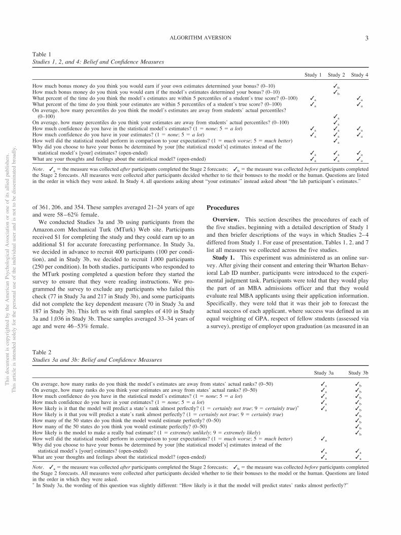
Table 1Studies 1, 2, and 4: Belief and Confidence Measures

Study 1 Study 2 Study 4

How much bonus money do you think you would earn if your own estimates determined your bonus? (0–10) ✓bHow much bonus money do you think you would earn if the model’s estimates determined your bonus? (0–10) ✓bWhat percent of the time do you think the model’s estimates are within 5 percentiles of a student’s true score? (0–100) ✓a ✓aWhat percent of the time do you think your estimates are within 5 percentiles of a student’s true score? (0–100) ✓a ✓aOn average, how many percentiles do you think the model’s estimates are away from students’ actual percentiles?(0–100) ✓a

On average, how many percentiles do you think your estimates are away from students’ actual percentiles? (0–100) ✓aHow much confidence do you have in the statistical model’s estimates? (1 ! none; 5 ! a lot) ✓a ✓a ✓aHow much confidence do you have in your estimates? (1 ! none; 5 ! a lot) ✓a ✓a ✓aHow well did the statistical model perform in comparison to your expectations? (1 ! much worse; 5 ! much better) ✓aWhy did you choose to have your bonus be determined by your [the statistical model’s] estimates instead of thestatistical model’s [your] estimates? (open-ended) ✓a ✓a ✓a

What are your thoughts and feelings about the statistical model? (open-ended) ✓a ✓a ✓a

Note. ✓a ! the measure was collected after participants completed the Stage 2 forecasts; ✓b ! the measure was collected before participants completedthe Stage 2 forecasts. All measures were collected after participants decided whether to tie their bonuses to the model or the human. Questions are listedin the order in which they were asked. In Study 4, all questions asking about “your estimates” instead asked about “the lab participant’s estimates.”

Table 2Studies 3a and 3b: Belief and Confidence Measures

Study 3a Study 3b

On average, how many ranks do you think the model’s estimates are away from states’ actual ranks? (0–50) ✓a ✓bOn average, how many ranks do you think your estimates are away from states’ actual ranks? (0–50) ✓a ✓bHow much confidence do you have in the statistical model’s estimates? (1 ! none; 5 ! a lot) ✓a ✓bHow much confidence do you have in your estimates? (1 ! none; 5 ! a lot) ✓a ✓bHow likely is it that the model will predict a state’s rank almost perfectly? (1 ! certainly not true; 9 ! certainly true)! ✓a ✓bHow likely is it that you will predict a state’s rank almost perfectly? (1 ! certainly not true; 9 ! certainly true) ✓bHow many of the 50 states do you think the model would estimate perfectly? (0–50) ✓bHow many of the 50 states do you think you would estimate perfectly? (0–50) ✓bHow likely is the model to make a really bad estimate? (1 ! extremely unlikely; 9 ! extremely likely) ✓bHow well did the statistical model perform in comparison to your expectations? (1 ! much worse; 5 ! much better) ✓aWhy did you choose to have your bonus be determined by your [the statistical model’s] estimates instead of thestatistical model’s [your] estimates? (open-ended) ✓a ✓a

What are your thoughts and feelings about the statistical model? (open-ended) ✓a ✓a

Note. ✓a ! the measure was collected after participants completed the Stage 2 forecasts; ✓b ! the measure was collected before participants completedthe Stage 2 forecasts. All measures were collected after participants decided whether to tie their bonuses to the model or the human. Questions are listedin the order in which they were asked.! In Study 3a, the wording of this question was slightly different: “How likely is it that the model will predict states’ ranks almost perfectly?”



3ALGORITHM AVERSION

annual poll of MBA students around the Unites States), and jobsuccess 2 years after graduation (measured by promotions andraises).Participants were then told that the admissions office had cre-

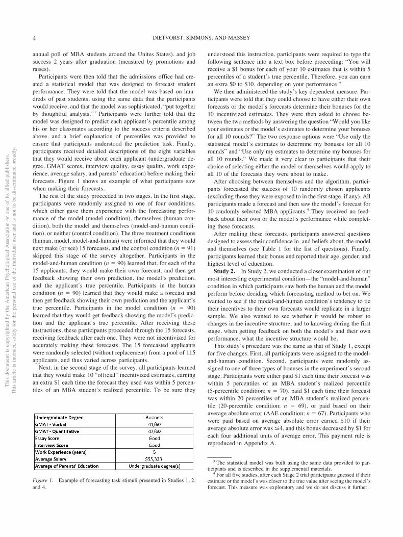
ated a statistical model that was designed to forecast studentperformance. They were told that the model was based on hun-dreds of past students, using the same data that the participantswould receive, and that the model was sophisticated, “put togetherby thoughtful analysts.”3 Participants were further told that themodel was designed to predict each applicant’s percentile amonghis or her classmates according to the success criteria describedabove, and a brief explanation of percentiles was provided toensure that participants understood the prediction task. Finally,participants received detailed descriptions of the eight variablesthat they would receive about each applicant (undergraduate de-gree, GMAT scores, interview quality, essay quality, work expe-rience, average salary, and parents’ education) before making theirforecasts. Figure 1 shows an example of what participants sawwhen making their forecasts.The rest of the study proceeded in two stages. In the first stage,

participants were randomly assigned to one of four conditions,which either gave them experience with the forecasting perfor-mance of the model (model condition), themselves (human con-dition), both the model and themselves (model-and-human condi-tion), or neither (control condition). The three treatment conditions(human, model, model-and-human) were informed that they wouldnext make (or see) 15 forecasts, and the control condition (n ! 91)skipped this stage of the survey altogether. Participants in themodel-and-human condition (n ! 90) learned that, for each of the15 applicants, they would make their own forecast, and then getfeedback showing their own prediction, the model’s prediction,and the applicant’s true percentile. Participants in the humancondition (n ! 90) learned that they would make a forecast andthen get feedback showing their own prediction and the applicant’strue percentile. Participants in the model condition (n ! 90)learned that they would get feedback showing the model’s predic-tion and the applicant’s true percentile. After receiving theseinstructions, these participants proceeded through the 15 forecasts,receiving feedback after each one. They were not incentivized foraccurately making these forecasts. The 15 forecasted applicantswere randomly selected (without replacement) from a pool of 115applicants, and thus varied across participants.Next, in the second stage of the survey, all participants learned

that they would make 10 “official” incentivized estimates, earningan extra $1 each time the forecast they used was within 5 percen-tiles of an MBA student’s realized percentile. To be sure they

understood this instruction, participants were required to type thefollowing sentence into a text box before proceeding: “You willreceive a $1 bonus for each of your 10 estimates that is within 5percentiles of a student’s true percentile. Therefore, you can earnan extra $0 to $10, depending on your performance.”We then administered the study’s key dependent measure. Par-

ticipants were told that they could choose to have either their ownforecasts or the model’s forecasts determine their bonuses for the10 incentivized estimates. They were then asked to choose be-tween the two methods by answering the question “Would you likeyour estimates or the model’s estimates to determine your bonusesfor all 10 rounds?” The two response options were “Use only thestatistical model’s estimates to determine my bonuses for all 10rounds” and “Use only my estimates to determine my bonuses forall 10 rounds.” We made it very clear to participants that theirchoice of selecting either the model or themselves would apply toall 10 of the forecasts they were about to make.After choosing between themselves and the algorithm, partici-

pants forecasted the success of 10 randomly chosen applicants(excluding those they were exposed to in the first stage, if any). Allparticipants made a forecast and then saw the model’s forecast for10 randomly selected MBA applicants.4 They received no feed-back about their own or the model’s performance while complet-ing these forecasts.After making these forecasts, participants answered questions

designed to assess their confidence in, and beliefs about, the modeland themselves (see Table 1 for the list of questions). Finally,participants learned their bonus and reported their age, gender, andhighest level of education.Study 2. In Study 2, we conducted a closer examination of our

most interesting experimental condition—the “model-and-human”condition in which participants saw both the human and the modelperform before deciding which forecasting method to bet on. Wewanted to see if the model-and-human condition’s tendency to tietheir incentives to their own forecasts would replicate in a largersample. We also wanted to see whether it would be robust tochanges in the incentive structure, and to knowing during the firststage, when getting feedback on both the model’s and their ownperformance, what the incentive structure would be.This study’s procedure was the same as that of Study 1, except

for five changes. First, all participants were assigned to the model-and-human condition. Second, participants were randomly as-signed to one of three types of bonuses in the experiment’s secondstage. Participants were either paid $1 each time their forecast waswithin 5 percentiles of an MBA student’s realized percentile(5-percentile condition; n ! 70), paid $1 each time their forecastwas within 20 percentiles of an MBA student’s realized percen-tile (20-percentile condition; n ! 69), or paid based on theiraverage absolute error (AAE condition; n ! 67). Participants whowere paid based on average absolute error earned $10 if theiraverage absolute error was !4, and this bonus decreased by $1 foreach four additional units of average error. This payment rule isreproduced in Appendix A.

3 The statistical model was built using the same data provided to par-ticipants and is described in the supplemental materials.4 For all five studies, after each Stage 2 trial participants guessed if their

estimate or the model’s was closer to the true value after seeing the model’sforecast. This measure was exploratory and we do not discuss it further.

Figure 1. Example of forecasting task stimuli presented in Studies 1, 2,and 4.




Third, unlike in Study 1, participants learned this payment rulejust before making the 15 unincentivized forecasts in the firststage. Thus, they were fully informed about the payment rule whileencoding their own and the model’s performance during the first15 trials. We implemented this design feature in Studies 3a and 3bas well.Fourth, participants completed a few additional confidence and

belief measures, some of which were asked immediately beforethey completed their Stage 2 forecasts (see Table 1). Participantsalso answered an exploratory block of questions asking them torate the relative competencies of the model and themselves on anumber of specific attributes. This block of questions, which wasalso included in the remaining studies, is listed in Table 7.Study 3a. Study 3a examined whether the results of Study 1

would replicate in a different forecasting domain and when themodel outperformed participants’ forecasts by a much wider mar-gin. As in Study 1, participants were randomly assigned to one offour conditions—model (n ! 101), human (n ! 105), model-and-human (n ! 99), and control (n ! 105)—which determinedwhether, in the first stage of the experiment, they saw the model’sforecasts, made their own forecasts, both, or neither.The Study 3a procedure was the same as Study 1 except for a

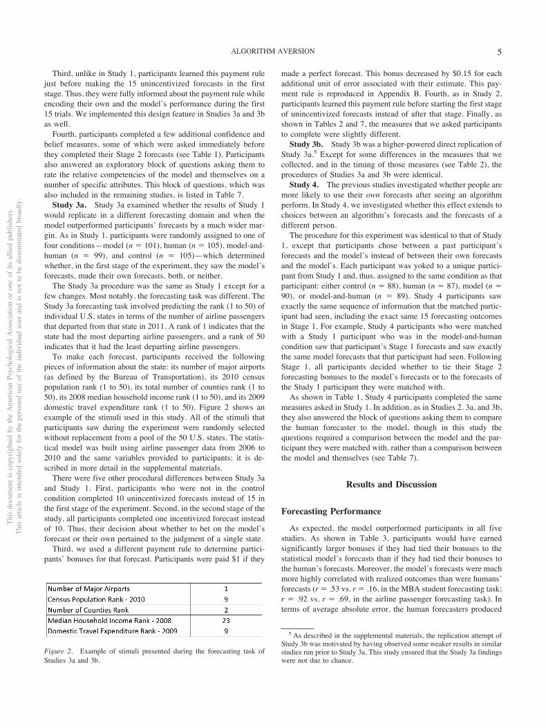
few changes. Most notably, the forecasting task was different. TheStudy 3a forecasting task involved predicting the rank (1 to 50) ofindividual U.S. states in terms of the number of airline passengersthat departed from that state in 2011. A rank of 1 indicates that thestate had the most departing airline passengers, and a rank of 50indicates that it had the least departing airline passengers.To make each forecast, participants received the following

pieces of information about the state: its number of major airports(as defined by the Bureau of Transportation), its 2010 censuspopulation rank (1 to 50), its total number of counties rank (1 to50), its 2008 median household income rank (1 to 50), and its 2009domestic travel expenditure rank (1 to 50). Figure 2 shows anexample of the stimuli used in this study. All of the stimuli thatparticipants saw during the experiment were randomly selectedwithout replacement from a pool of the 50 U.S. states. The statis-tical model was built using airline passenger data from 2006 to2010 and the same variables provided to participants; it is de-scribed in more detail in the supplemental materials.There were five other procedural differences between Study 3a

and Study 1. First, participants who were not in the controlcondition completed 10 unincentivized forecasts instead of 15 inthe first stage of the experiment. Second, in the second stage of thestudy, all participants completed one incentivized forecast insteadof 10. Thus, their decision about whether to bet on the model’sforecast or their own pertained to the judgment of a single state.Third, we used a different payment rule to determine partici-

pants’ bonuses for that forecast. Participants were paid $1 if they

made a perfect forecast. This bonus decreased by $0.15 for eachadditional unit of error associated with their estimate. This pay-ment rule is reproduced in Appendix B. Fourth, as in Study 2,participants learned this payment rule before starting the first stageof unincentivized forecasts instead of after that stage. Finally, asshown in Tables 2 and 7, the measures that we asked participantsto complete were slightly different.Study 3b. Study 3b was a higher-powered direct replication of

Study 3a.5 Except for some differences in the measures that wecollected, and in the timing of those measures (see Table 2), theprocedures of Studies 3a and 3b were identical.Study 4. The previous studies investigated whether people are

more likely to use their own forecasts after seeing an algorithmperform. In Study 4, we investigated whether this effect extends tochoices between an algorithm’s forecasts and the forecasts of adifferent person.The procedure for this experiment was identical to that of Study

1, except that participants chose between a past participant’sforecasts and the model’s instead of between their own forecastsand the model’s. Each participant was yoked to a unique partici-pant from Study 1 and, thus, assigned to the same condition as thatparticipant: either control (n ! 88), human (n ! 87), model (n !90), or model-and-human (n ! 89). Study 4 participants sawexactly the same sequence of information that the matched partic-ipant had seen, including the exact same 15 forecasting outcomesin Stage 1. For example, Study 4 participants who were matchedwith a Study 1 participant who was in the model-and-humancondition saw that participant’s Stage 1 forecasts and saw exactlythe same model forecasts that that participant had seen. FollowingStage 1, all participants decided whether to tie their Stage 2forecasting bonuses to the model’s forecasts or to the forecasts ofthe Study 1 participant they were matched with.As shown in Table 1, Study 4 participants completed the same

measures asked in Study 1. In addition, as in Studies 2, 3a, and 3b,they also answered the block of questions asking them to comparethe human forecaster to the model, though in this study thequestions required a comparison between the model and the par-ticipant they were matched with, rather than a comparison betweenthe model and themselves (see Table 7).

Results and Discussion

Forecasting Performance

As expected, the model outperformed participants in all fivestudies. As shown in Table 3, participants would have earnedsignificantly larger bonuses if they had tied their bonuses to thestatistical model’s forecasts than if they had tied their bonuses tothe human’s forecasts. Moreover, the model’s forecasts were muchmore highly correlated with realized outcomes than were humans’forecasts (r ! .53 vs. r ! .16, in the MBA student forecasting task;r ! .92 vs. r ! .69, in the airline passenger forecasting task). Interms of average absolute error, the human forecasters produced

5 As described in the supplemental materials, the replication attempt ofStudy 3b was motivated by having observed some weaker results in similarstudies run prior to Study 3a. This study ensured that the Study 3a findingswere not due to chance.

Figure 2. Example of stimuli presented during the forecasting task ofStudies 3a and 3b.



5ALGORITHM AVERSION

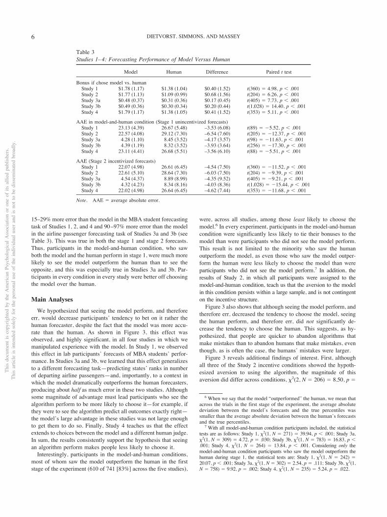
15–29% more error than the model in the MBA student forecastingtask of Studies 1, 2, and 4 and 90–97% more error than the modelin the airline passenger forecasting task of Studies 3a and 3b (seeTable 3). This was true in both the stage 1 and stage 2 forecasts.Thus, participants in the model-and-human condition, who sawboth the model and the human perform in stage 1, were much morelikely to see the model outperform the human than to see theopposite, and this was especially true in Studies 3a and 3b. Par-ticipants in every condition in every study were better off choosingthe model over the human.

Main AnalysesWe hypothesized that seeing the model perform, and therefore

err, would decrease participants’ tendency to bet on it rather thehuman forecaster, despite the fact that the model was more accu-rate than the human. As shown in Figure 3, this effect wasobserved, and highly significant, in all four studies in which wemanipulated experience with the model. In Study 1, we observedthis effect in lab participants’ forecasts of MBA students’ perfor-mance. In Studies 3a and 3b, we learned that this effect generalizesto a different forecasting task—predicting states’ ranks in numberof departing airline passengers—and, importantly, to a context inwhich the model dramatically outperforms the human forecasters,producing about half as much error in these two studies. Althoughsome magnitude of advantage must lead participants who see thealgorithm perform to be more likely to choose it—for example, ifthey were to see the algorithm predict all outcomes exactly right—the model’s large advantage in these studies was not large enoughto get them to do so. Finally, Study 4 teaches us that the effectextends to choices between the model and a different human judge.In sum, the results consistently support the hypothesis that seeingan algorithm perform makes people less likely to choose it.Interestingly, participants in the model-and-human conditions,

most of whom saw the model outperform the human in the firststage of the experiment (610 of 741 [83%] across the five studies),

were, across all studies, among those least likely to choose themodel.6 In every experiment, participants in the model-and-humancondition were significantly less likely to tie their bonuses to themodel than were participants who did not see the model perform.This result is not limited to the minority who saw the humanoutperform the model, as even those who saw the model outper-form the human were less likely to choose the model than wereparticipants who did not see the model perform.7 In addition, theresults of Study 2, in which all participants were assigned to themodel-and-human condition, teach us that the aversion to the modelin this condition persists within a large sample, and is not contingenton the incentive structure.Figure 3 also shows that although seeing the model perform, and

therefore err, decreased the tendency to choose the model, seeingthe human perform, and therefore err, did not significantly de-crease the tendency to choose the human. This suggests, as hy-pothesized, that people are quicker to abandon algorithms thatmake mistakes than to abandon humans that make mistakes, eventhough, as is often the case, the humans’ mistakes were larger.Figure 3 reveals additional findings of interest. First, although

all three of the Study 2 incentive conditions showed the hypoth-esized aversion to using the algorithm, the magnitude of thisaversion did differ across conditions, "2(2, N ! 206) ! 8.50, p !

6 When we say that the model “outperformed” the human, we mean thatacross the trials in the first stage of the experiment, the average absolutedeviation between the model’s forecasts and the true percentiles wassmaller than the average absolute deviation between the human’s forecastsand the true percentiles.7 With all model-and-human condition participants included, the statistical

tests are as follows: Study 1, "2(1, N ! 271) ! 39.94, p # .001; Study 3a,"2(1, N ! 309) ! 4.72, p ! .030; Study 3b, "2(1, N ! 783) ! 16.83, p #.001; Study 4, "2(1, N ! 264) ! 13.84, p # .001. Considering only themodel-and-human condition participants who saw the model outperform thehuman during stage 1, the statistical tests are: Study 1, "2(1, N ! 242) !20.07, p # .001; Study 3a, "2(1, N ! 302)! 2.54, p ! .111; Study 3b, "2(1,N ! 758) ! 9.92, p ! .002; Study 4, "2(1, N ! 235) ! 5.24, p ! .022.

Table 3Studies 1–4: Forecasting Performance of Model Versus Human

Model Human Difference Paired t test

Bonus if chose model vs. humanStudy 1 $1.78 (1.17) $1.38 (1.04) $0.40 (1.52) t(360) ! 4.98, p # .001Study 2 $1.77 (1.13) $1.09 (0.99) $0.68 (1.56) t(204) ! 6.26, p # .001Study 3a $0.48 (0.37) $0.31 (0.36) $0.17 (0.45) t(405) ! 7.73, p # .001Study 3b $0.49 (0.36) $0.30 (0.34) $0.20 (0.44) t(1,028) ! 14.40, p # .001Study 4 $1.79 (1.17) $1.38 (1.05) $0.41 (1.52) t(353) ! 5.11, p # .001

AAE in model-and-human condition (Stage 1 unincentivized forecasts)Study 1 23.13 (4.39) 26.67 (5.48) –3.53 (6.08) t(89) ! $5.52, p # .001Study 2 22.57 (4.08) 29.12 (7.30) –6.54 (7.60) t(205) ! $12.37, p # .001Study 3a 4.28 (1.10) 8.45 (3.52) –4.17 (3.57) t(98) ! $11.63, p # .001Study 3b 4.39 (1.19) 8.32 (3.52) –3.93 (3.64) t(256) ! $17.30, p # .001Study 4 23.11 (4.41) 26.68 (5.51) –3.56 (6.10) t(88) ! $5.51, p # .001

AAE (Stage 2 incentivized forecasts)Study 1 22.07 (4.98) 26.61 (6.45) –4.54 (7.50) t(360) ! $11.52, p # .001Study 2 22.61 (5.10) 28.64 (7.30) –6.03 (7.50) t(204) ! $9.39, p # .001Study 3a 4.54 (4.37) 8.89 (8.99) –4.35 (9.52) t(405) ! $9.21, p # .001Study 3b 4.32 (4.23) 8.34 (8.16) –4.03 (8.36) t(1,028) ! $15.44, p # .001Study 4 22.02 (4.98) 26.64 (6.45) –4.62 (7.44) t(353) ! $11.68, p # .001

Note. AAE ! average absolute error.




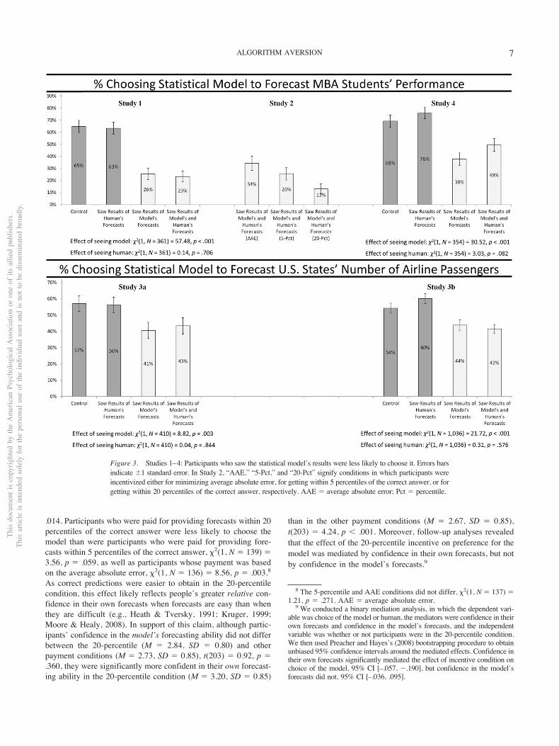
.014. Participants who were paid for providing forecasts within 20percentiles of the correct answer were less likely to choose themodel than were participants who were paid for providing fore-casts within 5 percentiles of the correct answer, "2(1, N ! 139) !3.56, p ! .059, as well as participants whose payment was basedon the average absolute error, "2(1, N ! 136) ! 8.56, p ! .003.8As correct predictions were easier to obtain in the 20-percentilecondition, this effect likely reflects people’s greater relative con-fidence in their own forecasts when forecasts are easy than whenthey are difficult (e.g., Heath & Tversky, 1991; Kruger, 1999;Moore & Healy, 2008). In support of this claim, although partic-ipants’ confidence in the model’s forecasting ability did not differbetween the 20-percentile (M ! 2.84, SD ! 0.80) and otherpayment conditions (M ! 2.73, SD ! 0.85), t(203) ! 0.92, p !.360, they were significantly more confident in their own forecast-ing ability in the 20-percentile condition (M ! 3.20, SD ! 0.85)

than in the other payment conditions (M ! 2.67, SD ! 0.85),t(203) ! 4.24, p # .001. Moreover, follow-up analyses revealedthat the effect of the 20-percentile incentive on preference for themodel was mediated by confidence in their own forecasts, but notby confidence in the model’s forecasts.9

8 The 5-percentile and AAE conditions did not differ, "2(1, N ! 137) !1.21, p ! .271. AAE ! average absolute error.9 We conducted a binary mediation analysis, in which the dependent vari-

able was choice of the model or human, the mediators were confidence in theirown forecasts and confidence in the model’s forecasts, and the independentvariable was whether or not participants were in the 20-percentile condition.We then used Preacher and Hayes’s (2008) bootstrapping procedure to obtainunbiased 95% confidence intervals around the mediated effects. Confidence intheir own forecasts significantly mediated the effect of incentive condition onchoice of the model, 95% CI [–.057, $.190], but confidence in the model’sforecasts did not, 95% CI [–.036, .095].

Figure 3. Studies 1–4: Participants who saw the statistical model’s results were less likely to choose it. Errors barsindicate %1 standard error. In Study 2, “AAE,” “5-Pct,” and “20-Pct” signify conditions in which participants wereincentivized either for minimizing average absolute error, for getting within 5 percentiles of the correct answer, or forgetting within 20 percentiles of the correct answer, respectively. AAE ! average absolute error; Pct ! percentile.



7ALGORITHM AVERSION

Additionally, although one must be cautious about making com-parisons across experiments, Figure 3 also shows that, acrossconditions, participants were more likely to bet on the modelagainst another participant (Study 4) than against themselves(Study 1). This suggests that algorithm aversion may be morepronounced among those whose forecasts the algorithm threatensto replace.

ConfidenceParticipants’ confidence ratings show an interesting pattern, one

that suggests that participants “learned” more from the model’smistakes than from the human’s (see Table 4). Whereas seeing thehuman perform did not consistently decrease confidence in thehuman’s forecasts—it did so significantly only in Study 4, seeingthe model perform significantly decreased participants’ confidencein the model’s forecasts in all four studies.10 Thus, seeing a modelmake relatively small mistakes consistently decreased confidencein the model, whereas seeing a human make relatively largemistakes did not consistently decrease confidence in the human.We tested whether confidence in the model’s or human’s fore-

casts significantly mediated the effect of seeing the model performon participants’ likelihood of choosing the model over the human.We conducted binary mediation analyses, setting choice of themodel or the human as the dependent variable (0 ! chose to tietheir bonus to the human; 1 ! chose to tie their bonus to themodel), whether or not participants saw the model perform asthe independent variable (0 ! control or human condition; 1 !model or model-and-human condition), and confidence in thehuman’s forecasts and confidence in the model’s forecasts asmediators. We used Preacher and Hayes’s (2008) bootstrappingprocedure to obtain unbiased 95% confidence intervals around themediated effects. In all cases, confidence in the model’s forecastssignificantly mediated the effect, whereas confidence in the humandid not.11It is interesting that reducing confidence in the model’s forecasts

seems to have led participants to abandon it, because participantswho saw the model perform were not more confident in thehuman’s forecasts than in the model’s. Whereas participants in thecontrol and human conditions were more confident in the model’sforecasts than in the human’s, participants in the model and model-

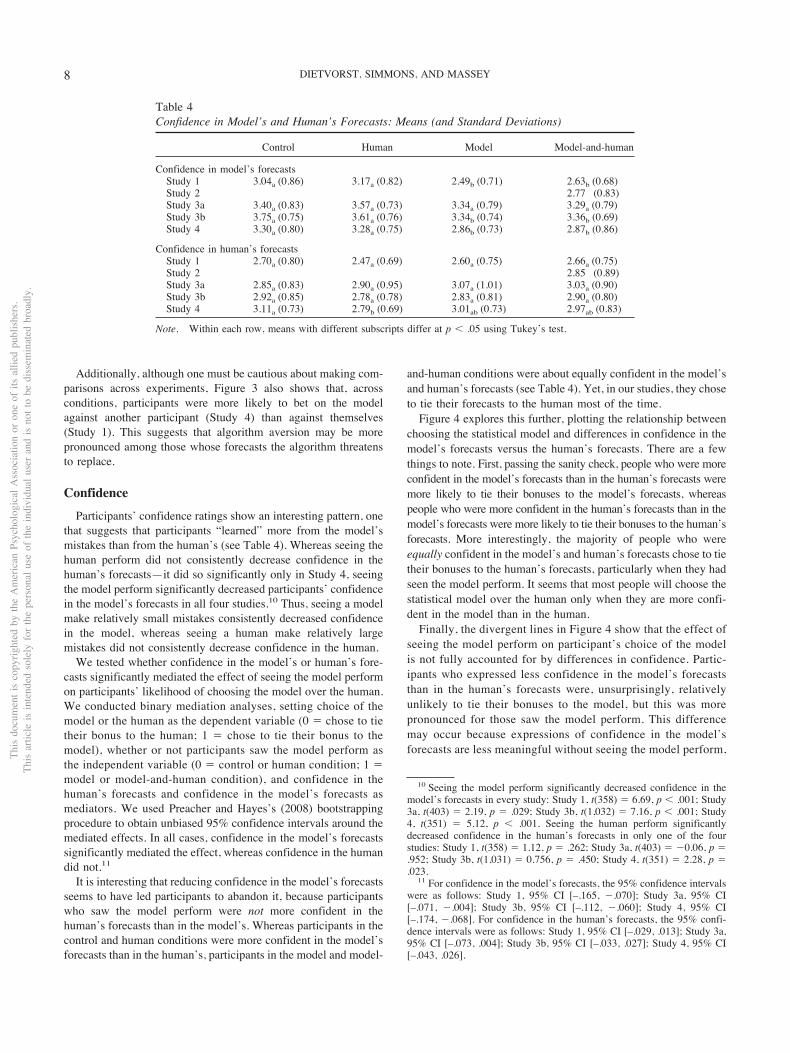
and-human conditions were about equally confident in the model’sand human’s forecasts (see Table 4). Yet, in our studies, they choseto tie their forecasts to the human most of the time.Figure 4 explores this further, plotting the relationship between

choosing the statistical model and differences in confidence in themodel’s forecasts versus the human’s forecasts. There are a fewthings to note. First, passing the sanity check, people who were moreconfident in the model’s forecasts than in the human’s forecasts weremore likely to tie their bonuses to the model’s forecasts, whereaspeople who were more confident in the human’s forecasts than in themodel’s forecasts were more likely to tie their bonuses to the human’sforecasts. More interestingly, the majority of people who wereequally confident in the model’s and human’s forecasts chose to tietheir bonuses to the human’s forecasts, particularly when they hadseen the model perform. It seems that most people will choose thestatistical model over the human only when they are more confi-dent in the model than in the human.Finally, the divergent lines in Figure 4 show that the effect of

seeing the model perform on participant’s choice of the modelis not fully accounted for by differences in confidence. Partic-ipants who expressed less confidence in the model’s forecaststhan in the human’s forecasts were, unsurprisingly, relativelyunlikely to tie their bonuses to the model, but this was morepronounced for those saw the model perform. This differencemay occur because expressions of confidence in the model’sforecasts are less meaningful without seeing the model perform,

10 Seeing the model perform significantly decreased confidence in themodel’s forecasts in every study: Study 1, t(358) ! 6.69, p # .001; Study3a, t(403) ! 2.19, p ! .029; Study 3b, t(1,032) ! 7.16, p # .001; Study4, t(351) ! 5.12, p # .001. Seeing the human perform significantlydecreased confidence in the human’s forecasts in only one of the fourstudies: Study 1, t(358) ! 1.12, p ! .262; Study 3a, t(403) ! $0.06, p !.952; Study 3b, t(1,031) ! 0.756, p ! .450; Study 4, t(351) ! 2.28, p !.023.11 For confidence in the model’s forecasts, the 95% confidence intervals

were as follows: Study 1, 95% CI [–.165, $.070]; Study 3a, 95% CI[–.071, $.004]; Study 3b, 95% CI [–.112, $.060]; Study 4, 95% CI[–.174, $.068]. For confidence in the human’s forecasts, the 95% confi-dence intervals were as follows: Study 1, 95% CI [–.029, .013]; Study 3a,95% CI [–.073, .004]; Study 3b, 95% CI [–.033, .027]; Study 4, 95% CI[–.043, .026].

Table 4Confidence in Model’s and Human’s Forecasts: Means (and Standard Deviations)

Control Human Model Model-and-human

Confidence in model’s forecastsStudy 1 3.04a (0.86) 3.17a (0.82) 2.49b (0.71) 2.63b (0.68)Study 2 2.77 (0.83)Study 3a 3.40a (0.83) 3.57a (0.73) 3.34a (0.79) 3.29a (0.79)Study 3b 3.75a (0.75) 3.61a (0.76) 3.34b (0.74) 3.36b (0.69)Study 4 3.30a (0.80) 3.28a (0.75) 2.86b (0.73) 2.87b (0.86)

Confidence in human’s forecastsStudy 1 2.70a (0.80) 2.47a (0.69) 2.60a (0.75) 2.66a (0.75)Study 2 2.85 (0.89)Study 3a 2.85a (0.83) 2.90a (0.95) 3.07a (1.01) 3.03a (0.90)Study 3b 2.92a (0.85) 2.78a (0.78) 2.83a (0.81) 2.90a (0.80)Study 4 3.11a (0.73) 2.79b (0.69) 3.01ab (0.73) 2.97ab (0.83)

Note. Within each row, means with different subscripts differ at p # .05 using Tukey’s test.




or because the confidence measure may fail to fully capturepeople’s disdain for a model that they see err. Whatever thecause, it is clear that seeing the model perform reduces thelikelihood of choosing the model, over and above the effect ithas on reducing confidence.

Beliefs

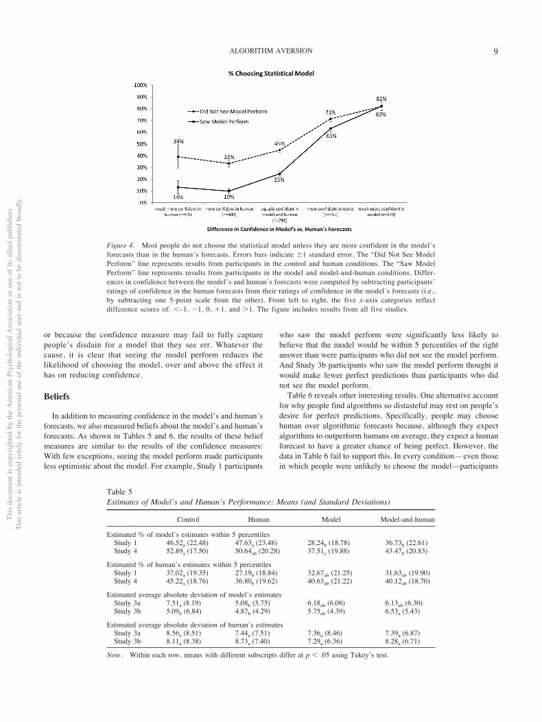
In addition to measuring confidence in the model’s and human’sforecasts, we also measured beliefs about the model’s and human’sforecasts. As shown in Tables 5 and 6, the results of these beliefmeasures are similar to the results of the confidence measures:With few exceptions, seeing the model perform made participantsless optimistic about the model. For example, Study 1 participants

who saw the model perform were significantly less likely tobelieve that the model would be within 5 percentiles of the rightanswer than were participants who did not see the model perform.And Study 3b participants who saw the model perform thought itwould make fewer perfect predictions than participants who didnot see the model perform.Table 6 reveals other interesting results. One alternative account

for why people find algorithms so distasteful may rest on people’sdesire for perfect predictions. Specifically, people may choosehuman over algorithmic forecasts because, although they expectalgorithms to outperform humans on average, they expect a humanforecast to have a greater chance of being perfect. However, thedata in Table 6 fail to support this. In every condition—even thosein which people were unlikely to choose the model—participants

Table 5Estimates of Model’s and Human’s Performance: Means (and Standard Deviations)


Estimated % of model’s estimates within 5 percentilesStudy 1 46.52a (22.48) 47.63a (23.48) 28.24b (18.78) 36.73b (22.61)Study 4 52.89a (17.50) 50.64ab (20.28) 37.51c (19.88) 43.47b (20.83)

Estimated % of human’s estimates within 5 percentilesStudy 1 37.02a (19.35) 27.19b (18.84) 32.67ab (21.25) 31.63ab (19.90)Study 4 45.22a (18.76) 36.80b (19.62) 40.63ab (21.22) 40.12ab (18.70)

Estimated average absolute deviation of model’s estimatesStudy 3a 7.51a (8.19) 5.08b (5.75) 6.18ab (6.06) 6.13ab (6.30)Study 3b 5.09b (6.84) 4.87b (4.29) 5.75ab (4.39) 6.53a (5.43)

Estimated average absolute deviation of human’s estimatesStudy 3a 8.56a (8.51) 7.44a (7.51) 7.36a (8.46) 7.39a (6.87)Study 3b 8.11a (8.38) 8.73a (7.40) 7.29a (6.36) 8.28a (6.71)


Figure 4. Most people do not choose the statistical model unless they are more confident in the model’sforecasts than in the human’s forecasts. Errors bars indicate %1 standard error. The “Did Not See ModelPerform” line represents results from participants in the control and human conditions. The “Saw ModelPerform” line represents results from participants in the model and model-and-human conditions. Differ-ences in confidence between the model’s and human’s forecasts were computed by subtracting participants’ratings of confidence in the human forecasts from their ratings of confidence in the model’s forecasts (i.e.,by subtracting one 5-point scale from the other). From left to right, the five x-axis categories reflectdifference scores of: #–1, $1, 0, &1, and '1. The figure includes results from all five studies.



9ALGORITHM AVERSION

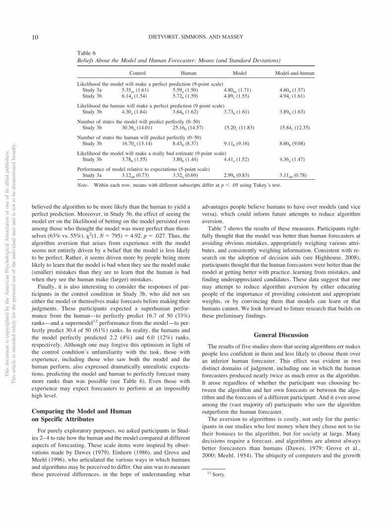
believed the algorithm to be more likely than the human to yield aperfect prediction. Moreover, in Study 3b, the effect of seeing themodel err on the likelihood of betting on the model persisted evenamong those who thought the model was more perfect than them-selves (63% vs. 55%), "2(1, N ! 795) ! 4.92, p ! .027. Thus, thealgorithm aversion that arises from experience with the modelseems not entirely driven by a belief that the model is less likelyto be perfect. Rather, it seems driven more by people being morelikely to learn that the model is bad when they see the model make(smaller) mistakes than they are to learn that the human is badwhen they see the human make (larger) mistakes.Finally, it is also interesting to consider the responses of par-

ticipants in the control condition in Study 3b, who did not seeeither the model or themselves make forecasts before making theirjudgments. These participants expected a superhuman perfor-mance from the human—to perfectly predict 16.7 of 50 (33%)ranks—and a supermodel12 performance from the model—to per-fectly predict 30.4 of 50 (61%) ranks. In reality, the humans andthe model perfectly predicted 2.2 (4%) and 6.0 (12%) ranks,respectively. Although one may forgive this optimism in light ofthe control condition’s unfamiliarity with the task, those withexperience, including those who saw both the model and thehuman perform, also expressed dramatically unrealistic expecta-tions, predicting the model and human to perfectly forecast manymore ranks than was possible (see Table 6). Even those withexperience may expect forecasters to perform at an impossiblyhigh level.

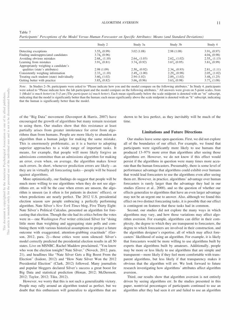
Comparing the Model and Humanon Specific AttributesFor purely exploratory purposes, we asked participants in Stud-

ies 2–4 to rate how the human and the model compared at differentaspects of forecasting. These scale items were inspired by obser-vations made by Dawes (1979), Einhorn (1986), and Grove andMeehl (1996), who articulated the various ways in which humansand algorithms may be perceived to differ. Our aim was to measurethese perceived differences, in the hope of understanding what

advantages people believe humans to have over models (and viceversa), which could inform future attempts to reduce algorithmaversion.Table 7 shows the results of these measures. Participants right-

fully thought that the model was better than human forecasters atavoiding obvious mistakes, appropriately weighing various attri-butes, and consistently weighing information. Consistent with re-search on the adoption of decision aids (see Highhouse, 2008),participants thought that the human forecasters were better than themodel at getting better with practice, learning from mistakes, andfinding underappreciated candidates. These data suggest that onemay attempt to reduce algorithm aversion by either educatingpeople of the importance of providing consistent and appropriateweights, or by convincing them that models can learn or thathumans cannot. We look forward to future research that builds onthese preliminary findings.

General DiscussionThe results of five studies show that seeing algorithms err makes

people less confident in them and less likely to choose them overan inferior human forecaster. This effect was evident in twodistinct domains of judgment, including one in which the humanforecasters produced nearly twice as much error as the algorithm.It arose regardless of whether the participant was choosing be-tween the algorithm and her own forecasts or between the algo-rithm and the forecasts of a different participant. And it even aroseamong the (vast majority of) participants who saw the algorithmoutperform the human forecaster.The aversion to algorithms is costly, not only for the partic-

ipants in our studies who lost money when they chose not to tietheir bonuses to the algorithm, but for society at large. Manydecisions require a forecast, and algorithms are almost alwaysbetter forecasters than humans (Dawes, 1979; Grove et al.,2000; Meehl, 1954). The ubiquity of computers and the growth

12 Sorry.

Table 6Beliefs About the Model and Human Forecaster: Means (and Standard Deviations)


Likelihood the model will make a perfect prediction (9-point scale)Study 3a 5.35ac (1.61) 5.59a (1.50) 4.80bc (1.71) 4.60b (1.57)Study 3b 6.14a (1.54) 5.72b (1.59) 4.89c (1.55) 4.94c (1.61)

Likelihood the human will make a perfect prediction (9-point scale)Study 3b 4.30a (1.84) 3.64b (1.62) 3.73b (1.61) 3.89b (1.63)

Number of states the model will predict perfectly (0–50)Study 3b 30.36a (14.01) 25.16b (14.57) 15.20c (11.83) 15.84c (12.35)

Number of states the human will predict perfectly (0–50)Study 3b 16.70a (13.14) 8.43b (8.37) 9.11b (9.16) 8.60b (9.08)

Likelihood the model will make a really bad estimate (9-point scale)Study 3b 3.78b (1.55) 3.80b (1.44) 4.41a (1.52) 4.36a (1.47)

Performance of model relative to expectations (5-point scale)Study 3a 3.12ab (0.73) 3.32a (0.69) 2.99b (0.83) 3.11ab (0.78)





of the “Big Data” movement (Davenport & Harris, 2007) haveencouraged the growth of algorithms but many remain resistantto using them. Our studies show that this resistance at leastpartially arises from greater intolerance for error from algo-rithms than from humans. People are more likely to abandon analgorithm than a human judge for making the same mistake.This is enormously problematic, as it is a barrier to adoptingsuperior approaches to a wide range of important tasks. Itmeans, for example, that people will more likely forgive anadmissions committee than an admissions algorithm for makingan error, even when, on average, the algorithm makes fewersuch errors. In short, whenever prediction errors are likely—asthey are in virtually all forecasting tasks—people will be biasedagainst algorithms.More optimistically, our findings do suggest that people will be

much more willing to use algorithms when they do not see algo-rithms err, as will be the case when errors are unseen, the algo-rithm is unseen (as it often is for patients in doctors’ offices), orwhen predictions are nearly perfect. The 2012 U.S. presidentialelection season saw people embracing a perfectly performingalgorithm. Nate Silver’s New York Times blog, Five Thirty Eight:Nate Silver’s Political Calculus, presented an algorithm for fore-casting that election. Though the site had its critics before the voteswere in—one Washington Post writer criticized Silver for “doinglittle more than weighting and aggregating state polls and com-bining them with various historical assumptions to project a futureoutcome with exaggerated, attention-grabbing exactitude” (Ger-son, 2012, para. 2)—those critics were soon silenced: Silver’smodel correctly predicted the presidential election results in all 50states. Live on MSNBC, Rachel Maddow proclaimed, “You knowwho won the election tonight? Nate Silver,” (Noveck, 2012, para.21), and headlines like “Nate Silver Gets a Big Boost From theElection” (Isidore, 2012) and “How Nate Silver Won the 2012Presidential Election” (Clark, 2012) followed. Many journalistsand popular bloggers declared Silver’s success a great boost forBig Data and statistical prediction (Honan, 2012; McDermott,2012; Taylor, 2012; Tiku, 2012).However, we worry that this is not such a generalizable victory.

People may rally around an algorithm touted as perfect, but wedoubt that this enthusiasm will generalize to algorithms that are

shown to be less perfect, as they inevitably will be much of thetime.

Limitations and Future DirectionsOur studies leave some open questions. First, we did not explore

all of the boundaries of our effect. For example, we found thatparticipants were significantly more likely to use humans thatproduced 13–97% more error than algorithms after seeing thosealgorithms err. However, we do not know if this effect wouldpersist if the algorithms in question were many times more accu-rate than the human forecasters. Presumably, there is some level ofperformance advantage that algorithms could exhibit over humansthat would lead forecasters to use the algorithms even after seeingthem err. However, in practice, algorithms’ advantage over humanforecasters is rarely larger than the advantage they had in ourstudies (Grove et al., 2000), and so the question of whether oureffects generalize to algorithms that have an even larger advantagemay not be an urgent one to answer. Also, although we found thiseffect on two distinct forecasting tasks, it is possible that our effectis contingent on features that these tasks had in common.Second, our studies did not explore the many ways in which

algorithms may vary, and how those variations may affect algo-rithm aversion. For example, algorithms can differ in their com-plexity, the degree to which they are transparent to forecasters, thedegree to which forecasters are involved in their construction, andthe algorithm designer’s expertise, all of which may affect fore-casters’ likelihood of using an algorithm. For example, it is likelythat forecasters would be more willing to use algorithms built byexperts than algorithms built by amateurs. Additionally, peoplemay be more or less likely to use algorithms that are simple andtransparent—more likely if they feel more comfortable with trans-parent algorithms, but less likely if that transparency makes itobvious that the algorithm will err. We look forward to futureresearch investigating how algorithms’ attributes affect algorithmaversion.Third, our results show that algorithm aversion is not entirely

driven by seeing algorithms err. In the studies presented in thispaper, nontrivial percentages of participants continued to use analgorithm after they had seen it err and failed to use an algorithm

Table 7Participants’ Perceptions of the Model Versus Human Forecaster on Specific Attributes: Means (and Standard Deviations)

Study 2 Study 3a Study 3b Study 4

Detecting exceptions 3.55h (0.99) 3.02 (1.08) 2.98 (1.08) 3.91h (0.97)Finding underappreciated candidates 3.74h (0.96) 4.04h (0.98)Avoiding obvious mistakes 2.68m (1.10) 2.64m (1.03) 2.62m (1.02) 2.55m (1.13)Learning from mistakes 3.91h (0.81) 3.74h (0.92) 3.67h (0.95) 3.81h (0.99)Appropriately weighing a candidate’squalities (state’s attributes) 2.98 (1.09) 2.50m (0.92) 2.34m (0.93) 2.81m (1.11)

Consistently weighing information 2.33m (1.10) 2.49m (1.00) 2.29m (0.98) 2.05m (1.02)Treating each student (state) individually 3.60h (1.02) 2.94 (1.02) 2.89m (1.02) 3.48h (1.25)Getting better with practice 3.85h (0.82) 3.66h (0.96) 3.63h (0.98) 3.77h (1.08)

Note. In Studies 2–3b, participants were asked to “Please indicate how you and the model compare on the following attributes.” In Study 4, participantswere asked to “Please indicate how the lab participant and the model compare on the following attributes.” All answers were given on 5-point scales, from1 (Model is much better) to 5 (I am [The participant is] much better). Each mean significantly below the scale midpoint is denoted with an “m” subscript,indicating that the model is significantly better than the human; each mean significantly above the scale midpoint is denoted with an “h” subscript, indicatingthat the human is significantly better than the model.



11ALGORITHM AVERSION

when they had not seen it err. This suggests that there are otherimportant drivers of algorithm aversion that we have not uncov-ered. Finally, our research has little to say about how best to reducealgorithm aversion among those who have seen the algorithm err.This is the next (and great) challenge for future research.

References

Arkes, H. R., Dawes, R. M., & Christensen, C. (1986). Factors influencingthe use of a decision rule in a probabilistic task. Organizational Behaviorand Human Decision Processes, 37, 93–110. http://dx.doi.org/10.1016/0749-5978(86)90046-4

Clark, D. (2012, November 7). How Nate Silver won the 2012 presidentialelection. Harvard Business Review Blog. Retrieved from http://blogs.hbr.org/cs/2012/11/how_nate_silver_won_the_2012_p.html

Davenport, T. H., & Harris, J. G. (2007). Competing on analytics: The newscience of winning. Boston, MA: Harvard Business Press.

Dawes, R. M. (1979). The robust beauty of improper linear models indecision making. American Psychologist, 34, 571–582. http://dx.doi.org/10.1037/0003-066X.34.7.571

Dawes, R. M., Faust, D., & Meehl, P. E. (1989). Clinical versus actuarialjudgment. Science, 243, 1668–1674. http://dx.doi.org/10.1126/science.2648573

Diab, D. L., Pui, S. Y., Yankelevich, M., & Highhouse, S. (2011). Layperceptions of selection decision aids in U.S. and non-U.S. samples.International Journal of Selection and Assessment, 19, 209–216. http://dx.doi.org/10.1111/j.1468-2389.2011.00548.x

Eastwood, J., Snook, B., & Luther, K. (2012). What people want from theirprofessionals: Attitudes toward decision-making strategies. Journal ofBehavioral Decision Making, 25, 458–468. http://dx.doi.org/10.1002/bdm.741

Einhorn, H. J. (1986). Accepting error to make less error. Journal ofPersonality Assessment, 50, 387–395. http://dx.doi.org/10.1207/s15327752jpa5003_8

Gerson, M. (2012, November 5). Michael Gerson: The trouble withObama’s silver lining. The Washington Post. Retrieved from http://www.washingtonpost.com/opinions/michael-gerson-the-trouble-with-obamas-silver-lining/2012/11/05/6b1058fe-276d-11e2-b2a0-ae18d6159439_story.html

Grove, W. M., & Meehl, P. E. (1996). Comparative efficiency of informal(subjective, impressionistic) and formal (mechanical, algorithmic) pre-diction procedures: The clinical-statistical controversy. Psychology,Public Policy, and Law, 2, 293–323. http://dx.doi.org/10.1037/1076-8971.2.2.293

Grove, W. M., Zald, D. H., Lebow, B. S., Snitz, B. E., & Nelson, C. (2000).Clinical versus mechanical prediction: A meta-analysis. PsychologicalAssessment, 12, 19–30. http://dx.doi.org/10.1037/1040-3590.12.1.19

Heath, C., & Tversky, A. (1991). Preference and belief: Ambiguity andcompetence in choice under uncertainty. Journal of Risk and Uncer-tainty, 4, 5–28. http://dx.doi.org/10.1007/BF00057884

Highhouse, S. (2008). Stubborn reliance on intuition and subjectivity inemployee selection. Industrial and Organizational Psychology: Per-spectives on Science and Practice, 1, 333–342. http://dx.doi.org/10.1111/j.1754-9434.2008.00058.x

Honan, D. (2012, November 7). The 2012 election: A big win for big data.Big Think. Retrieved from http://bigthink.com/think-tank/the-2012-election-a-big-win-for-big-data

Isidore, C. (2012, November 7). Nate Silver gets a big boost from theelection. CNN Money. Retrieved from http://money.cnn.com/2012/11/07/news/companies/nate-silver-election/index.html

Kruger, J. (1999). Lake Wobegon be gone! The “below-average effect” andthe egocentric nature of comparative ability judgments. Journal ofPersonality and Social Psychology, 77, 221–232. http://dx.doi.org/10.1037/0022-3514.77.2.221

McDermott, J. (2012, November 7). Nate Silver’s election predictions awin for big data, the New York Times. Ad Age. Retrieved from http://adage.com/article/campaign-trail/nate-silver-s-election-predictions-a-win-big-data-york-times/238182/

Meehl, P. E. (1954). Clinical versus statistical prediction: A theoreticalanalysis and review of the literature. Minneapolis, MN: University ofMinnesota Press.

Moore, D. A., & Healy, P. J. (2008). The trouble with overconfidence.Psychological Review, 115, 502–517. http://dx.doi.org/10.1037/0033-295X.115.2.502

Noveck, J. (2012, November 9). Nate Silver, pop culture star: After 2012election, statistician finds celebrity. Huffington Post. Retrieved fromhttp://www.huffingtonpost.com/2012/11/09 nate-silver-celebri-ty_n_2103761.html

Önkal, D., Goodwin, P., Thomson, M., Gönül, S., & Pollock, A. (2009).The relative influence of advice from human experts and statisticalmethods on forecast adjustments. Journal of Behavioral Decision Mak-ing, 22, 390–409. http://dx.doi.org/10.1002/bdm.637

Preacher, K. J., & Hayes, A. F. (2008). Asymptotic and resamplingstrategies for assessing and comparing indirect effects in multiple me-diator models. Behavior Research Methods, 40, 879–891. http://dx.doi.org/10.3758/BRM.40.3.879

Promberger, M., & Baron, J. (2006). Do patients trust computers? Journalof Behavioral Decision Making, 19, 455–468. http://dx.doi.org/10.1002/bdm.542

Shaffer, V. A., Probst, C. A., Merkle, E. C., Arkes, H. R., & Medow, M. A.(2013). Why do patients derogate physicians who use a computer-baseddiagnostic support system? Medical Decision Making, 33, 108–118.http://dx.doi.org/10.1177/0272989X12453501

Silver, N. (2012). The signal and the noise: Why so many predictionsfail–but some don’t. New York, NY: Penguin Press.

Taylor, C. (2012, November 7). Triumph of the nerds: Nate Silver wins in50 states. Mashable. Retrieved from http://mashable.com/2012/11/07/nate-silver-wins/

Tiku, N. (2012, November 7). Nate Silver’s sweep is a huge win for “BigData”. Beta Beat. Retrieved from http://betabeat.com/2012/11/nate-silver-predicton-sweep-presidential-election-huge-win-big-data/

(Appendices follow)




Appendix A

Payment Rule for Study 2

Participants in the average absolute error condition of Study 2 were paid as follows:• $10: within 4 percentiles of student’s actual percentile on average• $9: within 8 percentiles of student’s actual percentile on average• $8: within 12 percentiles of student’s actual percentile on average• $7: within 16 percentiles of student’s actual percentile on average• $6: within 20 percentiles of student’s actual percentile on average• $5: within 24 percentiles of student’s actual percentile on average• $4: within 28 percentiles of student’s actual percentile on average• $3: within 32 percentiles of student’s actual percentile on average• $2: within 36 percentiles of student’s actual percentile on average• $1: Within 40 percentiles of student’s actual percentile on average

Appendix B

Payment Rule for Studies 3a and 3b

Participants in Studies 3a and 3b were paid as follows:• $1.00: perfectly predict state’s actual rank• $0.85: within 1 rank of state’s actual rank• $0.70: within 2 ranks of state’s actual rank• $0.55: within 3 ranks of state’s actual rank• $0.40: within 4 ranks of state’s actual rank• $0.25: within 5 ranks of state’s actual rank• $0.10: within 6 ranks of state’s actual rank

Received July 6, 2014Revision received September 23, 2014

Accepted September 25, 2014 !



13ALGORITHM AVERSION

Documents

Algorithm Aversion: People Erroneously Avoid Algorithms ...opim.wharton.upenn.edu/risk/library/WPAF201410-AlgorthimAversion... · Algorithm Aversion: People Erroneously Avoid Algorithms