Algorithm Evaluation - NUS Computing - Homecs5240/lecture/evaluation.pdf · Colour Calibration Problem Deﬁnition PA3 Inputs Reference image R, colour of point pin Ris v∗(p). Target

Algorithm Evaluation

CS5240 Theoretical Foundations in Multimedia

Leow Wee Kheng

Department of Computer ScienceSchool of Computing

National University of Singapore

Leow Wee Kheng (NUS) Algorithm Evaluation 1 / 23

You Have Learned...

You Have Learned...

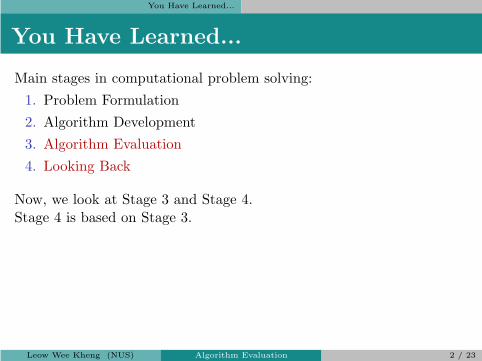
Main stages in computational problem solving:

1. Problem Formulation

2. Algorithm Development

3. Algorithm Evaluation

4. Looking Back

Now, we look at Stage 3 and Stage 4.Stage 4 is based on Stage 3.


Verification and Evaluation


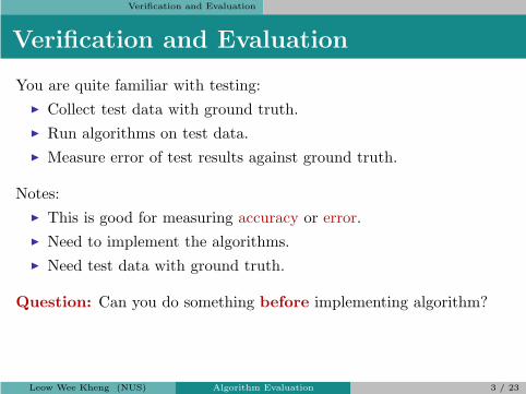
You are quite familiar with testing:

◮ Collect test data with ground truth.

◮ Run algorithms on test data.

◮ Measure error of test results against ground truth.

Notes:

◮ This is good for measuring accuracy or error.

◮ Need to implement the algorithms.

◮ Need test data with ground truth.

Question: Can you do something before implementing algorithm?



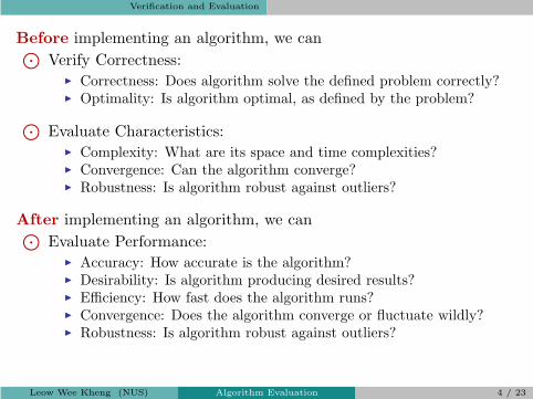
Before implementing an algorithm, we can⊙

Verify Correctness:◮ Correctness: Does algorithm solve the defined problem correctly?◮ Optimality: Is algorithm optimal, as defined by the problem?

⊙

Evaluate Characteristics:◮ Complexity: What are its space and time complexities?◮ Convergence: Can the algorithm converge?◮ Robustness: Is algorithm robust against outliers?

After implementing an algorithm, we can⊙

Evaluate Performance:◮ Accuracy: How accurate is the algorithm?◮ Desirability: Is algorithm producing desired results?◮ Efficiency: How fast does the algorithm runs?◮ Convergence: Does the algorithm converge or fluctuate wildly?◮ Robustness: Is algorithm robust against outliers?



Surprise! A correct and optimal algorithm may not be desirable!

If problem definition is not defined appropriately,algorithm can be correct and optimal as defined in problem definition,but producing undesired results.

Example: Can you name a simple example of the above?


Colour Calibration

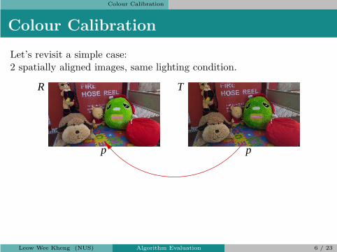
Colour Calibration

Let’s revisit a simple case:2 spatially aligned images, same lighting condition.

R T

p p


Colour Calibration

Problem Definition PA3Inputs

◮ Reference image R, colour of point p in R is v∗(p).

◮ Target image T , colour of point p in T is v(p).

◮ T and R are spatially aligned.

◮ T and R are captured under the same lighting condition.

Outputs

◮ Colour mapping function f from T to R.

Constraints

◮ f is a nonlinear function.

◮ For n points pi in T and R, the following colour difference isminimized:

n∑

i=1

‖f(v(pi))− v∗(pi)‖2. (1)


Colour Calibration

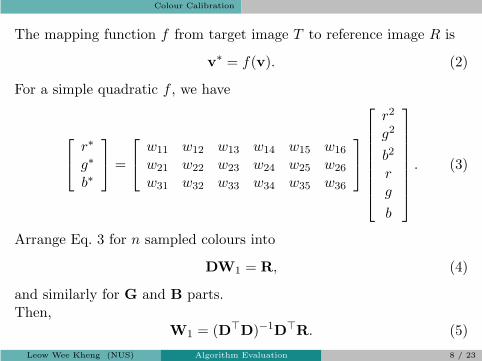
The mapping function f from target image T to reference image R is

v∗ = f(v). (2)

For a simple quadratic f , we have

r∗

g∗

b∗

=

w11 w12 w13 w14 w15 w16

w21 w22 w23 w24 w25 w26

w31 w32 w33 w34 w35 w36

r2

g2

b2

rg

b

. (3)

Arrange Eq. 3 for n sampled colours into

DW1 = R, (4)

and similarly for G and B parts.Then,

W1 = (D⊤D)−1D⊤R. (5)


Colour Calibration

Algorithm AA1: Colour Calibration

Input: Reference image R, target image T .Output: Parameters of colour mapping function f .

1 Sample n points pi, i = 1, . . . , n, in T and R; get v(pi), v∗(pi).

2 Use sampled colours to solve for parameters of f (Eq. 5).

Algorithm AA2: Colour Adjustment

Input: Target image T , computed f .Output: Resultant image T ′.

1 for each point p in T , do2 Compute v′(p) of T ′ using Eq. 3, with v∗ replaced by v′.


Colour Calibration

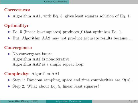
Correctness:

◮ Algorithm AA1, with Eq. 5, gives least squares solution of Eq. 1.

Optimality:

◮ Eq. 5 (linear least squares) produces f that optimizes Eq. 1.

◮ But, Algorithm AA2 may not produce accurate results because ...

Convergence:

◮ No convergence issue:Algorithm AA1 is non-iterative.Algorithm AA2 is a simple repeat loop.

Complexity: Algorithm AA1

◮ Step 1: Random sampling, space and time complexities are O(n).

◮ Step 2: What about Eq. 5, linear least squares?


Colour Calibration

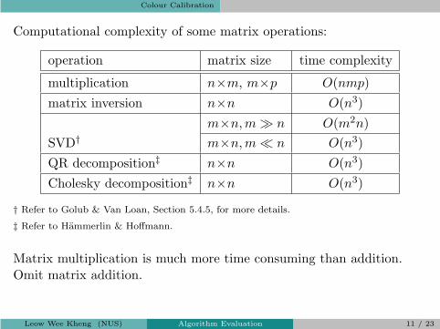
Computational complexity of some matrix operations:

operation matrix size time complexity

multiplication n×m, m×p O(nmp)

matrix inversion n×n O(n3)

m×n,m ≫ n O(m2n)

SVD† m×n,m ≪ n O(n3)

QR decomposition‡ n×n O(n3)

Cholesky decomposition‡ n×n O(n3)

† Refer to Golub & Van Loan, Section 5.4.5, for more details.

‡ Refer to Hammerlin & Hoffmann.

Matrix multiplication is much more time consuming than addition.Omit matrix addition.


Colour Calibration

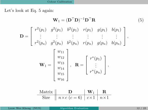
Let’s look at Eq. 5 again:

W1 = (D⊤D)−1D⊤R (5)

D =

r2(p1) g2(p1) b2(p1) r(p1) g(p1) b(p1)...

......

......

...r2(pn) g2(pn) b2(pn) r(pn) g(pn) b(pn)

,

W1 =

w11

w12

w13

w14

w15

w16

, R =

r∗(p1)...

r∗(pn)

,

Matrix D W1 R

Size n×c (c = 6) c×1 n×1


Colour Calibration

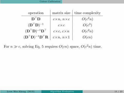
operation matrix size time complexity

D⊤D c×n, n×c O(c2n)

(D⊤D)−1 c×c O(c3)

(D⊤D)−1D⊤ c×c, c×n O(c2n)

(D⊤D)−1D⊤R c×n, n×1 O(cn)

For n ≫ c, solving Eq. 5 requires O(cn) space, O(c2n) time.


Colour Calibration


◮ Step 1: Random sampling: O(n) space and time complexities.

◮ Step 2: Linear least squares: O(cn) space, O(c2n) time complexity.

◮ Overvall: O(cn) space complexity, O(c2n) time complexity


◮ Eq. 3: O(c2) space and time complexities for each pixel.

◮ For m pixels in T , need m iterations.

◮ Overall: O(m) space (for m ≫ c2), O(mc2) time complexity.

Conclusion:

◮ Since c = 6 is small, the algorithms are quite efficient.

⊙

Analysis of Algorithm AB1 is straightforward [Homework].


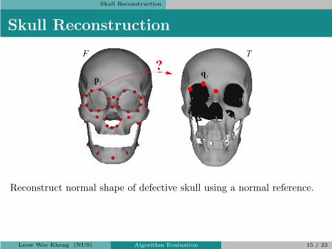
Skull Reconstruction


Reconstruct normal shape of defective skull using a normal reference.



Problem Definition PC2

⊙

Inputs:

◮ Reference model F , mesh points pi.

◮ Target model T with defective parts removed, mesh points qj .

⊙

Outputs:

◮ Point correspondence function c : R → T ∪ {∅},where ∅ denotes nothing.

◮ Shape change function f from pi to p′i.

◮ Resultant model R, mesh points f(pi).



⊙

Constraints:

◮ Close matching to T : main constraint, objective function

minimize∑

i,c(pi) 6=∅

‖f(pi)− c(pi)‖2.

◮ Minimize amount of no correspondence:

minimize |{i : c(pi) = ∅}|.

◮ R is normal:

minimize∑

i

‖f(pi)− pi‖2.



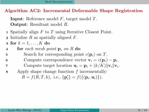
Algorithm AC2: Incremental Deformable Shape Registration

Input: Reference model F , target model T .Output: Resultant model R.

1 Spatially align F to T using Iterative Closest Point.2 Initialize R as spatially aligned F .3 for k = 1, . . . ,K do4 for each mesh point pi on R do5 Search for corresponding point c(pi) on T .6 Compute correspondence vector vi = c(pi)− pi.7 Compute target location ui = pi + (k/K)‖vi‖vi.

8 Apply shape change function f incrementally:R = f(R, T, k), i.e., {p′

i} = f({(pi,ui)}).



Correctness / Optimality:

◮ Similar to ICP, iterative shape change should satisfy Constraint 1.

◮ Satisfaction of Constraint 2 depends on correspondence search(Step 5).

◮ Constraint 3 is satisfied if shape change (Step 8) is not too drastic.

Convergence:

◮ ICP can converge [1].

◮ Steps 7 & 8 moves R closer and closer to T . Should converge.



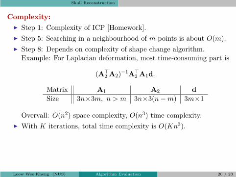
Complexity:

◮ Step 1: Complexity of ICP [Homework].

◮ Step 5: Searching in a neighbourhood of m points is about O(m).

◮ Step 8: Depends on complexity of shape change algorithm.Example: For Laplacian deformation, most time-consuming part is

(A⊤2 A2)

−1A⊤2 A1d.

Matrix A1 A2 d

Size 3n×3m, n > m 3n×3(n−m) 3m×1

Overvall: O(n2) space complexity, O(n3) time complexity.

◮ With K iterations, total time complexity is O(Kn3).


Look Back

Look Back

Look back at your problem definition and algorithms:

◮ Is there another way to solve the problem?

◮ Can you improve the problem definition and/or algorithm?

Algorithm AA1

◮ Which kind of nonlinear function gives best accuracy?

Algorithm AC2

◮ Is TSP or Laplacian deformation more appropriate?

◮ How to better ensure satisfaction of Constraints 2 & 3?


Summary

Summary

After developing an algorithm (before implementation), always

◮ Verify correctness, optimality of algorithm with problem definition.

◮ Evaluate convergence and complexity of algorithm.

Need to understand problem definition and algorithm well!

After implementing (programming) an algorithm, always

◮ Evaluate desirability of test results.

◮ Evaluate accuracy of algorithm against ground truth data.

◮ Evaluate efficiency, convergence, robustness of algorithm.

Look back

◮ Is there another way to solve the problem?

◮ Can you improve the problem definition and/or algorithm?


References

References

1. P. J. Besl and N. D. McKay. A method for registration of 3-D shapes.IEEE Trans. on Pattern Analysis and Machine Intelligence, 14(2),239–256, 1992.


Documents

Algorithm Evaluation - NUS Computing - Homecs5240/lecture/evaluation.pdf · Colour Calibration Problem Deﬁnition PA3 Inputs Reference image R, colour of point pin Ris v∗(p). Target