Algorithms and Data Structures: Minimum Spanning Trees I ... · Prim’s Algorithm Idea \Grow" an MST out of a single vertex by always adding \fringe" (neighbouring) edges of minimum

$Page 1: Algorithms and Data Structures: Minimum Spanning Trees I ... · Prim’s Algorithm Idea \Grow" an MST out of a single vertex by always adding \fringe" (neighbouring) edges of minimum$
Algorithms and Data Structures:Minimum Spanning Trees I and II - Prim’s Algorithm

ADS: lects 14 & 15 – slide 1 –

Weighted Graphs

Definition 1A weighted (directed or undirected graph) is a pair (G,W ) consisting ofa graph G = (V ,E ) and a weight function W : E → R.

In this lecture, we always assume that weights are non-negative, i.e., thatW (e) ≥ 0 for all e ∈ E .

Example

E D

BA

CHI

G

F

2.0

2.0

5.0

5.0

6.0

6.09.0

1.0

1.0

1.0

4.0

3.0

4.0

2.0 5.0


Representations of Weighted Graphs (as Matrices)

E D

BA

CHI

G

F

2.0

2.0

5.0

5.0

6.0

6.09.0

1.0

1.0

1.0

4.0

3.0

4.0

2.0 5.0

Adjacency Matrix

0 2.0 0 0 0 9.0 5.0 0 0

2.0 0 4.0 0 0 0 6.0 0 0

0 4.0 0 2.0 0 0 0 5.0 0

0 0 2.0 0 1.0 0 0 1.0 0

0 0 0 1.0 0 6.0 0 0 3.0

9.0 0 0 0 6.0 0 0 0 1.0

5.0 6.0 0 0 0 0 0 5.0 2.0

0 0 5.0 1.0 0 0 5.0 0 4.0

0 0 0 0 3.0 1.0 2.0 4.0 0


Representations of Weighted Graphs (Adjacency List)

E D

BA

CHI

G

F

2.0

2.0

5.0

5.0

6.0

6.09.0

1.0

1.0

1.0

4.0

3.0

4.0

2.0 5.0

Adjacency Lists

A

B

C

D

E

F

G

H

I

B G F

C G A

D H B

C H E

D I F

A I E

A B H I

G C D I

F G H E

2.0 5.0 9.0

4.0

2.0

2.0

1.0

9.0

1.0

5.0

5.0

6.0

5.0

1.0

3.0

1.0

6.0

5.0

2.0

4.0

2.0

1.0

6.0

5.0

4.0

6.0

1.0

2.0

4.0

3.0


Connecting Sites

ProblemGiven a collection of sites and costs of connecting them,find a minimum cost way of connecting all sites.

Our Graph Model

I Sites are vertices of a weighted graph, and (non-negative) weights ofthe edges represent the cost of connecting their endpoints.

I It is reasonable to assume that the graph is undirected andconnected.

I The cost of a subgraph is the sum of the costs of its edges.

I The problem is to find a subgraph of minimum cost that connectsall vertices.


Spanning Trees

G = (V ,E ) undirected connected graph and W weight function.H = (V H ,EH) with V H ⊆ V and EH ⊆ E subgraph of G.

I The weight of H is the number

W (H) =∑e∈EH

W (e).

I H is a spanning subgraph of G if V H = V .

Observation 2A connected spanning subgraph of minimum weight is a tree.


Minimum Spanning Trees

(G,W ) undirected connected weighted graph

Definition 3A minimum spanning tree (MST) of G is a connected spanningsubgraph T of G of minimum weight.

The minimum spanning tree problem:

Given: Undirected connected weighted graph (G,W )Output: An MST of G


Prim’s Algorithm

Idea“Grow” an MST out of a single vertex by always adding“fringe” (neighbouring) edges of minimum weight.

A fringe edge for a subtree T of a graph is an edge with exactly oneendpoint in T (so e = (u, v) with u ∈ T and v 6∈ T).

Algorithm Prim(G,W )

1. T ← one vertex tree with arbitrary vertex of G2. while there is a fringe edge do3. add fringe edge of minimum weight to T

4. return T

Note that this is another use of the greedy strategy.


Example

E D

BA

CHI

G

F

2.0

2.0

5.0

5.0

6.0

6.09.0

1.0

1.0

1.0

4.0

3.0

4.0

2.0 5.0


Correctness of Prim’s algorithm

1. Throughout the execution of Prim, T remains a tree.

Proof: To show this we need to show that throughout the execution of thealgorithm, T is (i) always connected and (ii) never contains a cycle.

(i) Only edges with an endpoint in T are added to T, so T remainsconnected.

(ii) We never add any edge which has both endpoints in T (we only allow asingle endpoint), so the algorithm will never construct a cycle.


Correctness of Prim’s algorithm (cont’d)

2. All vertices will eventually be added to T.

Proof: by contradiction ... (depends on our assumption that the graph G

was connected.)

I Suppose w is a vertex that never gets added to T (as usual, in proofby contradiction, we suppose the opposite of what we want).

I Let v = v0e1v1e2...vn = w be a path from some vertex v inside T tow (we know such a path must exist, because G is connected). Let vibe the first vertex on this path that never got added to T.

I After vi−1 was added to T, ei = (vi−1, vi ) would have become a fringeedge. Also, it would have remained as a fringe edge unless vi wasadded to T.

I So eventually vi must have been added, because Prims algorithm onlystops if there are no fringe edges. So our assumption was wrong. Sowe must have w in T for every vertex w .



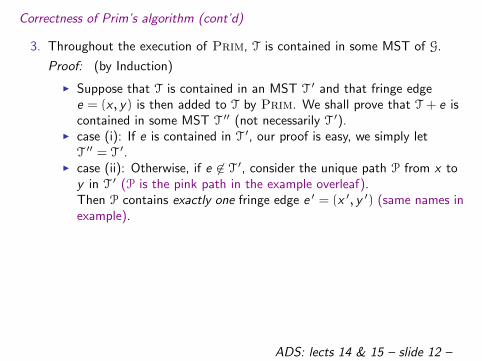
3. Throughout the execution of Prim, T is contained in some MST of G.

Proof: (by Induction)

I Suppose that T is contained in an MST T ′ and that fringe edgee = (x , y) is then added to T by Prim. We shall prove that T + e iscontained in some MST T ′′ (not necessarily T ′).

I case (i): If e is contained in T ′, our proof is easy, we simply letT ′′ = T ′.

I case (ii): Otherwise, if e 6∈ T ′, consider the unique path P from x toy in T ′ (P is the pink path in the example overleaf).Then P contains exactly one fringe edge e ′ = (x ′, y ′) (same names inexample).



T’(overall blue tree)

T(partial MST)

y’’

x’’ xy

x’

y’

Define T’’ to be T’ + (x,y) − (x’,y’)

("drop (x’,y’) and add (x,y)")

e

e’



3. case (ii) cont’d

I Then W (e) ≤W (e ′).(otherwise e ′ would definitely have been added before e)

I Let T ′′ = T ′ + e − e ′.I T ′′ is a tree.

Why? Well, we drop e ′ = (x ′, y ′), which splits the global MST Tinto two components: T ′

x ′ and the other subtree T ′y ′ = T ′ \ T ′

x ′ .We know x and y are now in different components after this split,because we have broken the unique path P between x and y in T ′.Hence we can add e = (x , y) to re-join T ′

x ′ and T ′y ′ without making a

cycle.T ′′ has the same vertices as T ′, thus it is a spanning tree.

I Moreover, W (T ′′) = W (T ′) + W (e) − W (e ′), and because we knowW (e) ≤W (e ′), this gives W (T ′′) ≤W (T ′), thus T ′′ is also a MST.


Towards an Implementation

Improvement

I Instead of fringe edges, we think about adding fringe vertices to thetree

I A fringe vertex is a vertex y not in T that is an endpoint of a fringeedge.

I The weight of a fringe vertex y is

min{W (e) | e = (x , y) a fringe edge}

(ie, the best weight that could “bring y into the MST”)

I To be able to recover the tree, every time we “bring a fringe vertexy into the tree”, we store its parent in the tree.

We will store the fringe vertices in a priority queue.


Priority Queues with Decreasing Key

A Priority Queue is an ADT for storing a collection of elements with anassociated key. The following methods are supported:

I Insert(e, k): Insert element e with key k .

I Get-Min(): Return an element with minimum key; an error occursif the priority queue is empty.

I Extract-Min(): Return and remove an element with minimumkey; an error if the priority queue is empty.

I Is-Empty(): Return true if the priority queue is empty and falseotherwise.

To update the keys during the execution of Prim, we need priority queuessupporting the following additional method:

I Decrease-Key(e, k): Set the key of e to k and update thepriority queue. It is assumed that k is smaller than of equal to theold key of e.


Implementation of Prim’s Algorithm

Algorithm Prim(G,W )

1. Initialise parent array π:π[v ]← nil for all vertices v

2. Initialise weight array:weight[v ]←∞ for all v

3. Initialise inMST array:inMST[v ]← false for all v

4. Initialise priority queue Q

5. v ← arbitrary vertex of G

6. Q.Insert(v , 0)

7. weight[v ] = 0;

8. while not(Q.Is-Empty()) do

9. y ← Q.Extract-Min()

10. inMST[y ]← true

11. for all z adjacent to y do

12. Relax(y,z)

13. return π

Algorithm Relax(y , z)

1. w ←W (y , z)

2. if weight[z ] =∞ then

3. weight[z ]← w

4. π[z ]← y

5. Q.Insert(z ,w)

6. else if (w < weight[z ] and

7. not (inMST[z ])) then

8. weight[z ]← w

9. π[z ]← y

10. Q.Decrease Key(z ,w)


Analysis of Prim’s algorithm

Let n be the number of vertices and m the number of edges of the inputgraph.

I Lines 1-7, 13 of Prim require Θ(n) time altogether.

I Q will extract each of the n vertices of G once. Thus the loop atlines 8-12 is iterated n times.Thus, disregarding (for now) the time to execute the inner loop(lines 11-12) the execution of the loop requires time

Θ(n · TExtract-Min(n)

)I The inner loop is executed at most once for each edge (and at least

once for each edge). So its execution requires time

Θ(m · TRelax(n,m)

).


Analysis of Prim’s algorithm (Relax)

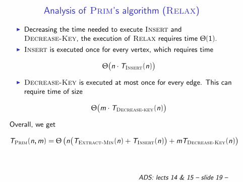
I Decreasing the time needed to execute Insert andDecrease-Key, the execution of Relax requires time Θ(1).

I Insert is executed once for every vertex, which requires time

Θ(n · TInsert(n)

)I Decrease-Key is executed at most once for every edge. This can

require time of size

Θ(m · TDecrease-key(n)

)Overall, we get

TPrim(n,m) = Θ(n(TExtract-Min(n) + TInsert(n)

)+ mTDecrease-Key(n)

)


Priority Queue Implementations

I Array: Elements simply stored in an array.

I Heap: Elements are stored in a binary heap (see Inf2B (ADS note7), [CLRS] Section 6.5)

I Fibonacci Heap: Sophisticated variant of the simple binary heap (see[CLRS] Chapters 19 and 20)

method running time

Array Heap Fibonacci Heap

Insert Θ(1) Θ(lg n) Θ(1)

Extract-Min Θ(n) Θ(lg n) Θ(lg n)

Decrease-Key Θ(1) Θ(lg n) Θ(1) (amortised)


Running-time of Prim

TPrim(n,m) = Θ(n(TExtract-Min(n) + TInsert(n)

)+ mTDecrease-Key(n)

)Which Priority Queue implementation?

I With array implementation of priority queue:

TPrim(n,m) = Θ(n2).

I With heap implementation of priority queue:

TPrim(n,m) = Θ((n + m) lg(n)).

I With Fibonacci heap implementation of priority queue:

TPrim(n,m) = Θ(n lg(n) + m).

(n being the number of vertices and m the number of edges)


Remarks

I The Fibonacci heap implementation is mainly of theoretical interest.It is not much used in practice because it is very complicated andthe constants hidden in the Θ-notation are large.

I For dense graphs with m = Θ(n2), the array implementation isprobably the best, because it is so simple.

I For sparser graphs with m ∈ O( n2

lg n ), the heap implementation is agood alternative, since it is still quite simple, but more efficient forsmaller m.Instead of using binary heaps, the use of d-ary heaps for some d ≥ 1can speed up the algorithm (see [Sedgewick] for a discussion ofpractical implementations of Prims algorithm).


Reading Assignment

[CLRS] Chapter 23.

Problems

1. Exercises 23.1-1, 23.1-2, 23.1-4 of [CLRS]

2. In line 3 of Prim’s algorithm, there may be more than one fringeedge of minimum weight. Suppose we add all these minimum edgesin one step. Does the algorithm still compute a MST?

3. Prove that our implementation of Prim’s algorithm on slide 6 iscorrect - ie, that it computes an MST. What is the differencebetween this and the suggested algorithm of Problem 4?


Documents

Algorithms and Data Structures: Minimum Spanning Trees I ... · Prim’s Algorithm Idea \Grow" an MST out of a single vertex by always adding \fringe" (neighbouring) edges of minimum