Algorithms for Classification: Notes by Gregory Piatetsky

Algorithms for Classification:

Notes by Gregory Piatetsky

22

Basic methods. Outline:

Simplicity first: 1R

Naïve Bayes

33

Task: Given a set of pre-classified examples, build a model or classifier to classify new cases.

Supervised learning: classes are known for the examples used to build the classifier.

A classifier can be a set of rules, a decision tree, a neural network, etc.

Typical applications: credit approval, direct marketing, fraud detection, medical diagnosis, …..

Classification

44

Simplicity first

Simple algorithms often work very well!

There are many kinds of simple structure, eg: One attribute does all the work

All attributes contribute equally & independently

A weighted linear combination might do

Instance-based: use a few prototypes

Use simple logical rules

Success of method depends on the domain

witten&eibe

55

Inferring rudimentary rules

1R: learns a 1-level decision tree I.e., rules that all test one particular attribute

Basic version One branch for each value

Each branch assigns most frequent class

Error rate: proportion of instances that don’t belong to the majority class of their corresponding branch

Choose attribute with lowest error rate

(assumes nominal attributes)

witten&eibe

66

Pseudo-code for 1R

For each attribute,

For each value of the attribute, make a rule as follows:

count how often each class appears

find the most frequent class

make the rule assign that class to this attribute-value

Calculate the error rate of the rules

Choose the rules with the smallest error rate

Note: “missing” is treated as a separate attribute value

witten&eibe

77

Evaluating the weather attributes

Attribute Rules Errors Total errors

Outlook Sunny No 2/5 4/14

Overcast Yes 0/4

Rainy Yes 2/5

Temp Hot No* 2/4 5/14

Mild Yes 2/6

Cool Yes 1/4

Humidity High No 3/7 4/14

Normal Yes 1/7

Windy False Yes 2/8 5/14

True No* 3/6

Outlook Temp Humidity

Windy Play

Sunny Hot High False No

Sunny Hot High True No

Overcast Hot High False Yes

Rainy Mild High False Yes

Rainy Cool Normal False Yes

Rainy Cool Normal True No

Overcast Cool Normal True Yes

Sunny Mild High False No

Sunny Cool Normal False Yes

Rainy Mild Normal False Yes

Sunny Mild Normal True Yes

Overcast Mild High True Yes

Overcast Hot Normal False Yes

Rainy Mild High True No

* indicates a tie

witten&eibe

88

Dealing withnumeric attributes

Discretize numeric attributes

Divide each attribute’s range into intervals Sort instances according to attribute’s values

Place breakpoints where the class changes(the majority class)

This minimizes the total error

Example: temperature from weather data

64 65 68 69 70 71 72 72 75 75 80 81 83 85

Yes | No | Yes Yes Yes | No No Yes | Yes Yes | No | Yes Yes | No

Outlook Temperature Humidity Windy Play

Sunny 85 85 False No

Sunny 80 90 True No

Overcast 83 86 False Yes

Rainy 75 80 False Yes

… … … … …

witten&eibe

99

The problem of overfitting

This procedure is very sensitive to noise One instance with an incorrect class label will probably

produce a separate interval

Also: time stamp attribute will have zero errors

Simple solution:enforce minimum number of instances in majority class per interval

witten&eibe

1010

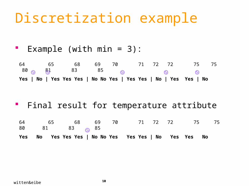
Discretization example

Example (with min = 3):

Final result for temperature attribute

64 65 68 69 70 71 72 72 75 75 80 81 83 85

Yes | No | Yes Yes Yes | No No Yes | Yes Yes | No | Yes Yes | No

64 65 68 69 70 71 72 72 75 75 80 81 83 85

Yes No Yes Yes Yes | No No Yes Yes Yes | No Yes Yes No

witten&eibe

1111

With overfitting avoidance

Resulting rule set:

Attribute Rules Errors Total errors

Outlook Sunny No 2/5 4/14

Overcast Yes 0/4

Rainy Yes 2/5

Temperature 77.5 Yes 3/10 5/14

> 77.5 No* 2/4

Humidity 82.5 Yes 1/7 3/14

> 82.5 and 95.5 No 2/6

> 95.5 Yes 0/1

Windy False Yes 2/8 5/14

True No* 3/6

witten&eibe

1313

Bayesian (Statistical) modeling

“Opposite” of 1R: use all the attributes

Two assumptions: Attributes are equally important

statistically independent (given the class value) I.e., knowing the value of one attribute says nothing

about the value of another(if the class is known)

Independence assumption is almost never correct!

But … this scheme works well in practice

witten&eibe

1414

Probabilities for weather dataOutlook Temperature Humidity Windy Play

Yes No Yes No Yes No Yes No Yes No

Sunny 2 3 Hot 2 2 High 3 4 False 6 2 9 5

Overcast

4 0 Mild 4 2 Normal 6 1 True 3 3

Rainy 3 2 Cool 3 1

Sunny 2/9 3/5 Hot 2/9 2/5 High 3/9 4/5 False 6/9 2/5 9/14

5/14

Overcast

4/9 0/5 Mild 4/9 2/5 Normal 6/9 1/5 True 3/9 3/5

Rainy 3/9 2/5 Cool 3/9 1/5

Outlook Temp Humidity Windy Play




Rainy Mild High False Yes

Rainy Cool Normal False Yes

Rainy Cool Normal True No

Overcast Cool Normal True Yes

Sunny Mild High False No

Sunny Cool Normal False Yes


Sunny Mild Normal True Yes

Overcast Mild High True Yes

Overcast Hot Normal False Yes

Rainy Mild High True Nowitten&eibe

1515

Probabilities for weather data

Outlook Temp. Humidity Windy Play

Sunny Cool High True ?

A new day: Likelihood of the two classes

For “yes” = 2/9 3/9 3/9 3/9 9/14 = 0.0053

For “no” = 3/5 1/5 4/5 3/5 5/14 = 0.0206

Conversion into a probability by normalization:

P(“yes”) = 0.0053 / (0.0053 + 0.0206) = 0.205

P(“no”) = 0.0206 / (0.0053 + 0.0206) = 0.795



Sunny 2 3 Hot 2 2 High 3 4 False 6 2 9 5

Overcast

4 0 Mild 4 2 Normal 6 1 True 3 3

Rainy 3 2 Cool 3 1

Sunny 2/9 3/5 Hot 2/9 2/5 High 3/9 4/5 False 6/9 2/5 9/14

5/14

Overcast

4/9 0/5 Mild 4/9 2/5 Normal 6/9 1/5 True 3/9 3/5

Rainy 3/9 2/5 Cool 3/9 1/5

witten&eibe

1616

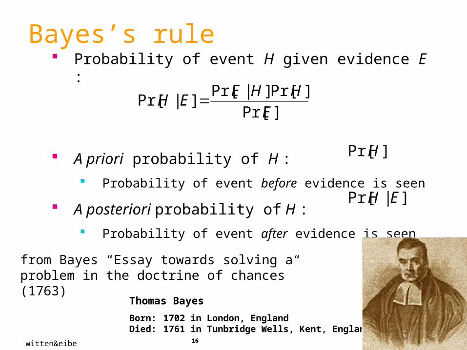
Bayes’s rule Probability of event H given evidence E :

A priori probability of H : Probability of event before evidence is seen

A posteriori probability of H : Probability of event after evidence is seen

]Pr[]Pr[]|Pr[

]|Pr[E

HHEEH

]|Pr[ EH

]Pr[H

Thomas Bayes

Born: 1702 in London, EnglandDied: 1761 in Tunbridge Wells, Kent, England

witten&eibe

from Bayes “Essay towards solving a problem in the doctrine of chances” (1763)

1717

Naïve Bayes for classification

Classification learning: what’s the probability of the class given an instance? Evidence E = instance

Event H = class value for instance

Naïve assumption: evidence splits into parts (i.e. attributes) that are independent

]Pr[

]Pr[]|Pr[]|Pr[]|Pr[]|Pr[ 11

E

HHEHEHEEH n

witten&eibe

1818

Weather data example


Sunny Cool High True ?Evidence E

Probability ofclass “yes”

]|Pr[]|Pr[ yesSunnyOutlookEyes ]|Pr[ yesCooleTemperatur

]|Pr[ yesHighHumidity ]|Pr[ yesTrueWindy

]Pr[

]Pr[

E

yes

]Pr[149

93

93

93

92

E

witten&eibe

1919

The “zero-frequency problem”

What if an attribute value doesn’t occur with every class value?(e.g. “Humidity = high” for class “yes”)

Probability will be zero!

A posteriori probability will also be zero!(No matter how likely the other values are!)

Remedy: add 1 to the count for every attribute value-class combination (Laplace estimator)

Result: probabilities will never be zero!(also: stabilizes probability estimates)

0]|Pr[ Eyes

0]|Pr[ yesHighHumidity

witten&eibe

2020

*Modified probability estimates

In some cases adding a constant different from 1 might be more appropriate

Example: attribute outlook for class yes

Weights don’t need to be equal (but they must sum to 1)

9

3/2

9

3/4

9

3/3

Sunny Overcast Rainy

92 1p

9

4 2p

9

3 3p

witten&eibe

2121

Missing values Training: instance is not included in

frequency count for attribute value-class combination

Classification: attribute will be omitted from calculation

Example: Outlook Temp. Humidity Windy Play

? Cool High True ?

Likelihood of “yes” = 3/9 3/9 3/9 9/14 = 0.0238

Likelihood of “no” = 1/5 4/5 3/5 5/14 = 0.0343

P(“yes”) = 0.0238 / (0.0238 + 0.0343) = 41%

P(“no”) = 0.0343 / (0.0238 + 0.0343) = 59%

witten&eibe

2222

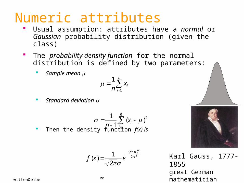
Numeric attributes Usual assumption: attributes have a normal or

Gaussian probability distribution (given the class)

The probability density function for the normal distribution is defined by two parameters: Sample mean

Standard deviation

Then the density function f(x) is

n

iix

n 1

1

n

iix

n 1

2)(1

1

2

2

2

)(

21

)(

x

exf

witten&eibe

Karl Gauss, 1777-1855great German mathematician

2323

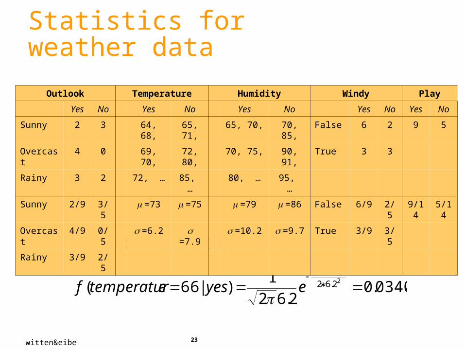
Statistics forweather data

Example density value:

0340.02.62

1)|66(

2

2

2.62

)7366(

eyesetemperaturf



Sunny 2 3 64, 68, 65, 71,

65, 70, 70, 85, False 6 2 9 5

Overcast

4 0 69, 70, 72, 80,

70, 75, 90, 91, True 3 3

Rainy 3 2 72, … 85, …

80, … 95, …

Sunny 2/9 3/5 =73 =75 =79 =86 False 6/9 2/5 9/14

5/14

Overcast

4/9 0/5 =6.2 =7.9

=10.2 =9.7 True 3/9 3/5

Rainy 3/9 2/5

witten&eibe

2424

Classifying a new day

A new day:

Missing values during training are not included in calculation of mean and standard deviation


Sunny 66 90 true ?

Likelihood of “yes” = 2/9 0.0340 0.0221 3/9 9/14 = 0.000036

Likelihood of “no” = 3/5 0.0291 0.0380 3/5 5/14 = 0.000136

P(“yes”) = 0.000036 / (0.000036 + 0. 000136) = 20.9%

P(“no”) = 0.000136 / (0.000036 + 0. 000136) = 79.1%

witten&eibe

2525

Naïve Bayes: discussion

Naïve Bayes works surprisingly well (even if independence assumption is clearly violated)

Why? Because classification doesn’t require accurate probability estimates as long as maximum probability is assigned to correct class

However: adding too many redundant attributes will cause problems (e.g. identical attributes)

Note also: many numeric attributes are not normally distributed ( kernel density estimators)

witten&eibe

2626

Naïve Bayes Extensions

Improvements: select best attributes (e.g. with greedy

search)

often works as well or better with just a fraction of all attributes

Bayesian Networks

witten&eibe

2727

Summary

OneR – uses rules based on just one attribute

Naïve Bayes – use all attributes and Bayes rules to estimate probability of the class given an instance.

Simple methods frequently work well, but … Complex methods can be better (as we will see)

Classification:

Decision Trees

2929

Outline

Top-Down Decision Tree Construction

Choosing the Splitting Attribute

Information Gain and Gain Ratio

3030

DECISION TREE

An internal node is a test on an attribute.

A branch represents an outcome of the test, e.g., Color=red.

A leaf node represents a class label or class label distribution.

At each node, one attribute is chosen to split training examples into distinct classes as much as possible

A new case is classified by following a matching path to a leaf node.

3131

Weather Data: Play or not Play?

Outlook Temperature Humidity Windy Play?

sunny hot high false No

sunny hot high true No

overcast hot high false Yes

rain mild high false Yes

rain cool normal false Yes

rain cool normal true No

overcast cool normal true Yes

sunny mild high false No

sunny cool normal false Yes

rain mild normal false Yes

sunny mild normal true Yes

overcast mild high true Yes

overcast hot normal false Yes

rain mild high true No

Note:Outlook is theForecast,no relation to Microsoftemail program

3232

overcast

high normal falsetrue

sunny rain

No NoYes Yes

Yes

Example Tree for “Play?”

Outlook

HumidityWindy

3333

Building Decision Tree [Q93]

Top-down tree construction At start, all training examples are at the root.

Partition the examples recursively by choosing one attribute each time.

Bottom-up tree pruning Remove subtrees or branches, in a bottom-up

manner, to improve the estimated accuracy on new cases.

3434


At each node, available attributes are evaluated on the basis of separating the classes of the training examples. A Goodness function is used for this purpose.

Typical goodness functions: information gain (ID3/C4.5)

information gain ratio

gini index

witten&eibe

3535

Which attribute to select?

witten&eibe

3636

A criterion for attribute selection Which is the best attribute?

The one which will result in the smallest tree

Heuristic: choose the attribute that produces the “purest” nodes

Popular impurity (disuniformity) criteria:

Gini Index

Information gain

Strategy: choose attribute that results in greatest information gain

witten&eibe

3737

If a data set T contains examples from n classes, gini index, gini(T) is defined as

where pj is the relative frequency of class j in T.

gini(T) is minimized if the classes in T are skewed.

*CART Splitting Criteria: Gini Index

3838

After splitting T into two subsets T1 and T2 with sizes N1 and N2, the gini index of the split data is defined as

The attribute providing smallest ginisplit(T) is chosen to split the node.

*Gini Index

3939

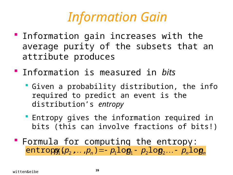
Information Gain Information gain increases with the

average purity of the subsets that an attribute produces

Information is measured in bits Given a probability distribution, the info

required to predict an event is the distribution’s entropy

Entropy gives the information required in bits (this can involve fractions of bits!)

Formula for computing the entropy:nnn ppppppppp logloglog),,,entropy( 221121

witten&eibe

4040

Claude Shannon, who has died aged 84, perhaps more than anyone laid the groundwork for today’s digital revolution. His exposition of information theory, stating that all information could be represented mathematically as a succession of noughts and ones, facilitated the digital manipulation of data without which today’s information society would be unthinkable.

Shannon’s master’s thesis, obtained in 1940 at MIT, demonstrated that problem solving could be achieved by manipulating the symbols 0 and 1 in a process that could be carried out automatically with electrical circuitry. That dissertation has been hailed as one of the most significant master’s theses of the 20th century. Eight years later, Shannon published another landmark paper, A Mathematical Theory of Communication, generally taken as his most important scientific contribution.

Born: 30 April 1916Died: 23 February 2001

“Father of information theory”

Shannon applied the same radical approach to cryptography research, in which he later became a consultant to the US government.

Many of Shannon’s pioneering insights were developed before they could be applied in practical form. He was truly a remarkable man, yet unknown to most of the world.witten&eibe

*Claude Shannon

4141

Example: attribute “Outlook”, 1

witten&eibe

Outlook Temperature Humidity Windy Play?

sunny hot high false No

sunny hot high true No

overcast hot high false Yes

rain mild high false Yes

rain cool normal false Yes

rain cool normal true No

overcast cool normal true Yes

sunny mild high false No

sunny cool normal false Yes

rain mild normal false Yes

sunny mild normal true Yes

overcast mild high true Yes

overcast hot normal false Yes

rain mild high true No

4242

Example: attribute “Outlook”, 2

“ Outlook” = “Sunny”:

“Outlook” = “Overcast”:

“Outlook” = “Rainy”:

Expected information for attribute:

bits 971.0)5/3log(5/3)5/2log(5/25,3/5)entropy(2/)info([2,3]

bits 0)0log(0)1log(10)entropy(1,)info([4,0]


Note: log(0) is not defined, but we evaluate 0*log(0) as zero

971.0)14/5(0)14/4(971.0)14/5([3,2])[4,0],,info([3,2] bits 693.0

witten&eibe

4343

Computing the information gain Information gain:

(information before split) – (information after split)

Compute for attribute “Humidity”

0.693-0.940[3,2])[4,0],,info([2,3]-)info([9,5])Outlook"gain(" bits 247.0

witten&eibe

4444

Example: attribute “Humidity”

“ Humidity” = “High”:

“Humidity” = “Normal”:

Expected information for attribute:

Information Gain:



592.0)14/7(985.0)14/7([6,1]),info([3,4] bits 79.0

0.1520.788-0.940[6,1]),info([3,4]-)info([9,5]

4545

Computing the information gain Information gain:

(information before split) – (information after split)

Information gain for attributes from weather data:

0.693-0.940[3,2])[4,0],,info([2,3]-)info([9,5])Outlook"gain(" bits 247.0

bits 247.0)Outlook"gain(" bits 029.0)e"Temperaturgain("

bits 152.0)Humidity"gain(" bits 048.0)Windy"gain("

witten&eibe

4646

Continuing to split

bits 571.0)e"Temperaturgain(" bits 971.0)Humidity"gain("

bits 020.0)Windy"gain("

witten&eibe

4747

The final decision tree

Note: not all leaves need to be pure; sometimes identical instances have different classes

Splitting stops when data can’t be split any further

witten&eibe

5050

Highly-branching attributes

Problematic: attributes with a large number of values (extreme case: ID code)

Subsets are more likely to be pure if there is a large number of values Information gain is biased towards choosing

attributes with a large number of values

This may result in overfitting (selection of an attribute that is non-optimal for prediction)

witten&eibe

5151

Weather Data with ID code

ID Outlook Temperature Humidity Windy Play?

A sunny hot high false No

B sunny hot high true No

C overcast hot high false Yes

D rain mild high false Yes

E rain cool normal false Yes

F rain cool normal true No

G overcast cool normal true Yes

H sunny mild high false No

I sunny cool normal false Yes

J rain mild normal false Yes

K sunny mild normal true Yes

L overcast mild high true Yes

M overcast hot normal false Yes

N rain mild high true No

5252

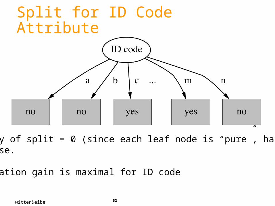
Split for ID Code Attribute

Entropy of split = 0 (since each leaf node is “pure”, having onlyone case.

Information gain is maximal for ID code

witten&eibe

5353

Gain ratio

Gain ratio: a modification of the information gain that reduces its bias on high-branch attributes

Gain ratio should be Large when data is evenly spread Small when all data belong to one branch

Gain ratio takes number and size of branches into account when choosing an attribute It corrects the information gain by taking the intrinsic

information of a split into account (i.e. how much info do we need to tell which branch an instance belongs to)

witten&eibe

5454

.||

||2

log||||

),(SiS

SiS

ASnfoIntrinsicI

.),(

),(),(ASnfoIntrinsicI

ASGainASGainRatio

Gain Ratio and Intrinsic Info.

Intrinsic information: entropy of distribution of instances into branches

Gain ratio (Quinlan’86) normalizes info gain by:

5555

Computing the gain ratio

Example: intrinsic information for ID code

Importance of attribute decreases as intrinsic information gets larger

Example of gain ratio:

Example:

bits 807.3)14/1log14/1(14),1[1,1,(info

)Attribute"info("intrinsic_)Attribute"gain("

)Attribute"("gain_ratio

246.0bits 3.807bits 0.940

)ID_code"("gain_ratio

witten&eibe

5656

Gain ratios for weather data

Outlook Temperature

Info: 0.693 Info: 0.911

Gain: 0.940-0.693 0.247 Gain: 0.940-0.911 0.029

Split info: info([5,4,5]) 1.577 Split info: info([4,6,4])

1.362

Gain ratio: 0.247/1.577

0.156 Gain ratio: 0.029/1.362

0.021

Humidity Windy

Info: 0.788 Info: 0.892

Gain: 0.940-0.788 0.152 Gain: 0.940-0.892 0.048

Split info: info([7,7]) 1.000 Split info: info([8,6]) 0.985

Gain ratio: 0.152/1 0.152 Gain ratio: 0.048/0.985

0.049

witten&eibe

5757

Discussion

Algorithm for top-down induction of decision trees (“ID3”) was developed by Ross Quinlan Gain ratio just one modification of this basic algorithm

Led to development of C4.5, which can deal with numeric attributes, missing values, and noisy data

Similar approach: CART (to be covered later)

There are many other attribute selection criteria! (But almost no difference in accuracy of result.)

5858

Summary

Top-Down Decision Tree Construction


Information Gain biased towards attributes with a large number of values

Gain Ratio takes number and size of branches into account when choosing an attribute

Machine Learning in Real World:

C4.5

6060

Outline

Handling Numeric Attributes Finding Best Split(s)

Dealing with Missing Values

Pruning Pre-pruning, Post-pruning, Error Estimates

From Trees to Rules

6161

Industrial-strength algorithms

For an algorithm to be useful in a wide range of real-world applications it must: Permit numeric attributes

Allow missing values

Be robust in the presence of noise

Be able to approximate arbitrary concept descriptions (at least in principle)

Basic schemes need to be extended to fulfill these requirements

witten & eibe

6262

C4.5 History

ID3, CHAID – 1960s

C4.5 innovations (Quinlan): permit numeric attributes

deal sensibly with missing values

pruning to deal with for noisy data

C4.5 - one of best-known and most widely-used learning algorithms Last research version: C4.8, implemented in Weka as J4.8

(Java)

Commercial successor: C5.0 (available from Rulequest)

6363

Numeric attributes Standard method: binary splits

E.g. temp < 45

Unlike nominal attributes,every attribute has many possible split points

Solution is straightforward extension: Evaluate info gain (or other measure)

for every possible split point of attribute

Choose “best” split point

Info gain for best split point is info gain for attribute

Computationally more demanding

witten & eibe

6464

Weather data – nominal valuesOutlook Temperature Humidity Windy Play





… … … … …

If outlook = sunny and humidity = high then play = no

If outlook = rainy and windy = true then play = no

If outlook = overcast then play = yes

If humidity = normal then play = yes

If none of the above then play = yes

witten & eibe

6565

Weather data - numericOutlook Temperature Humidity Windy Play

Sunny 85 85 False No

Sunny 80 90 True No

Overcast 83 86 False Yes

Rainy 75 80 False Yes

… … … … …

If outlook = sunny and humidity > 83 then play = no

If outlook = rainy and windy = true then play = no

If outlook = overcast then play = yes

If humidity < 85 then play = yes

If none of the above then play = yes

6666

Example Binary Split on temperature attribute:

E.g. temperature 71.5: yes/4, no/2temperature 71.5: yes/5, no/3

Info([4,2],[5,3])= 6/14 info([4,2]) + 8/14 info([5,3]) = 0.939 bits

Place split points halfway between values

Can evaluate all split points in one pass!

64 65 68 69 70 71 72 72 75 75 80 81 83 85

Yes No Yes Yes Yes No No Yes Yes Yes No Yes Yes No

witten & eibe

6767

Avoid repeated sorting!

Sort instances by the values of the numeric attribute Time complexity for sorting: O (n log n)

Q. Does this have to be repeated at each node of the tree?

A: No! Sort order for children can be derived from sort order for parent Time complexity of derivation: O (n)

Drawback: need to create and store an array of sorted indices for each numeric attribute

witten & eibe

6868

More speeding up

Entropy only needs to be evaluated between points of different classes (Fayyad & Irani, 1992)

64 65 68 69 70 71 72 72 75 75 80 81 83 85

Yes No Yes Yes Yes No No Yes Yes Yes No Yes Yes No

Potential optimal breakpoints

Breakpoints between values of the same class cannotbe optimal

valueclass

X

6969

Binary vs. multi-way splits Splitting (multi-way) on a nominal attribute exhausts

all information in that attribute Nominal attribute is tested (at most) once on any path in

the tree

Not so for binary splits on numeric attributes! Numeric attribute may be tested several times along a

path in the tree

Disadvantage: tree is hard to read

Remedy: pre-discretize numeric attributes, or

use multi-way splits instead of binary ones

witten & eibe

7070

Missing as a separate value Missing value denoted “?” in C4.X

Simple idea: treat missing as a separate value

Q: When this is not appropriate?

A: When values are missing due to different reasons Example 1: gene expression could be missing

when it is very high or very low

Example 2: field IsPregnant=missing for a male patient should be treated differently (no) than for a female patient of age 25 (unknown)

7171

Missing values - advanced

Split instances with missing values into pieces A piece going down a branch receives a weight

proportional to the popularity of the branch

weights sum to 1

Info gain works with fractional instances use sums of weights instead of counts

During classification, split the instance into pieces in the same way Merge probability distribution using weights

witten & eibe

7272

Pruning Goal: Prevent overfitting to noise in the data

Two strategies for “pruning” the decision tree: Postpruning - take a fully-grown decision tree and

discard unreliable parts

Prepruning - stop growing a branch when information becomes unreliable

Postpruning preferred in practice—prepruning can “stop too early”

7373

From trees to rules – simple Simple way: one rule for each leaf

C4.5rules: greedily prune conditions from each rule if this reduces its estimated error Can produce duplicate rules

Check for this at the end

Then look at each class in turn

consider the rules for that class

find a “good” subset (guided by MDL)

Then rank the subsets to avoid conflicts

Finally, remove rules (greedily) if this decreases error on the training data

witten & eibe

7474

C4.5rules: choices and options

C4.5 rules slow for large and noisy datasets

Commercial version C5.0 rules uses a different technique Much faster and a bit more accurate

C4.5 has two parameters Confidence value (default 25%):

lower values incur heavier pruning

Minimum number of instances in the two most popular branches (default 2)

witten & eibe

7575

Summary

Decision Trees splits – binary, multi-way split criteria – entropy, gini, … missing value treatment pruning rule extraction from trees

Both C4.5 and CART are robust tools No method is always superior –

experiment!

witten & eibe

Documents

Algorithms for Classification: Notes by Gregory Piatetsky