Algorithms for estimating and reconstructing recombination in

populations

Dan Gusfield

UC Davis

Different parts of this work are joint with Satish Eddhu, CharlesLangley, Dean Hickerson, Yun Song, Yufeng Wu, Z. Ding

Triangle - North Carolina State, Feb 19, 2007

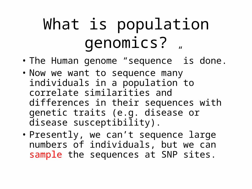
What is population genomics?

• The Human genome “sequence” is done.• Now we want to sequence many individuals

in a population to correlate similarities and differences in their sequences with genetic traits (e.g. disease or disease susceptibility).

• Presently, we can’t sequence large numbers of individuals, but we can sample the sequences at SNP sites.

SNP Data

• A SNP is a Single Nucleotide Polymorphism - a site in the genome where two different nucleotides appear with sufficient frequency in the population (say each with 5% frequency or more). Hence binary data.

• SNP maps have been compiled with a density of about 1 site per 1000.

• SNP data is what is mostly collected in populations - it is much cheaper to collect than full sequence data, and focuses on variation in the population, which is what is of interest.

Haplotype Map Project: HAPMAP

• NIH lead project ($100M) to find common SNP haplotypes (“SNP sequences”) in the Human population.

• Association mapping: HAPMAP used to try to associate genetic-influenced diseases with specific SNP haplotypes, to either find causal haplotypes, or to find the region near causal mutations.

• The key to the logic of Association mapping is historical recombination in populations. Nature has done the experiments, now we try to make sense of the results.

The Perfect Phylogeny Model for SNP sequences

00000

1

2

4

3

510100

1000001011

00010

01010

12345sitesAncestral sequence

Extant sequences at the leaves

Site mutations on edgesThe tree derives the set M:1010010000010110101000010

Only one mutation per siteallowed.

Classic NASC: Arrange the sequences in a matrix. Then (with no duplicate columns), the sequences can be generated on a unique perfect phylogeny if and only if no two columns (sites) contain all four pairs:

0,0 and 0,1 and 1,0 and 1,1

This is the 4-Gamete Test

When can a set of sequences be derived on a perfect phylogeny?

A richer model

00000

1

2

4

3

510100

1000001011

00010

01010

12345101001000001011010100001010101 added

Pair 4, 5 fails the fourgamete-test. The sites 4, 5``conflict”.

Real sequence histories often involve recombination.

M

10100 01011

5

10101

The first 4 sites come from P (Prefix) and the sitesfrom 5 onward come from S (Suffix).

P S

Sequence Recombination

A recombination of P and S at recombination point 5.

Single crossover recombination

Network with Recombination: ARG

00000

1

2

4

3

510100

1000001011

00010

01010

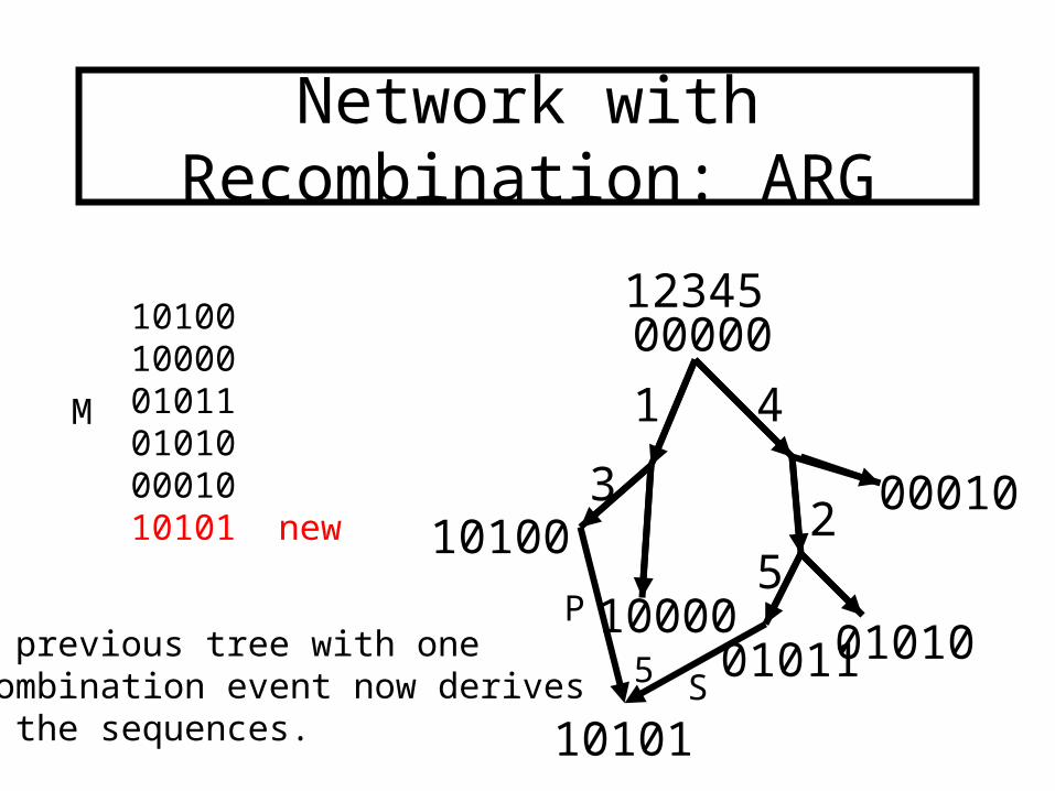
12345101001000001011010100001010101 new

10101

The previous tree with onerecombination event now derivesall the sequences.

5

P

S

M

An illustration of why we are interested in recombination:

Association Mapping of Complex Diseases Using

ARGs

Association Mapping

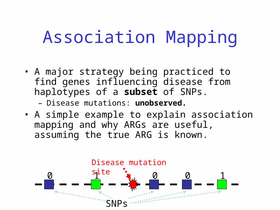
• A major strategy being practiced to find genes influencing disease from haplotypes of a subset of SNPs.– Disease mutations: unobserved.

• A simple example to explain association mapping and why ARGs are useful, assuming the true ARG is known.

0 1 0 0 1

Disease mutation site

SNPs

00000

52

3

2

4S

P

PS

1

4

a:00010

b:10010

c:00100

10010

01100

d:10100

e:01100

00101

01101

f:01101

g:00101

00100

00010

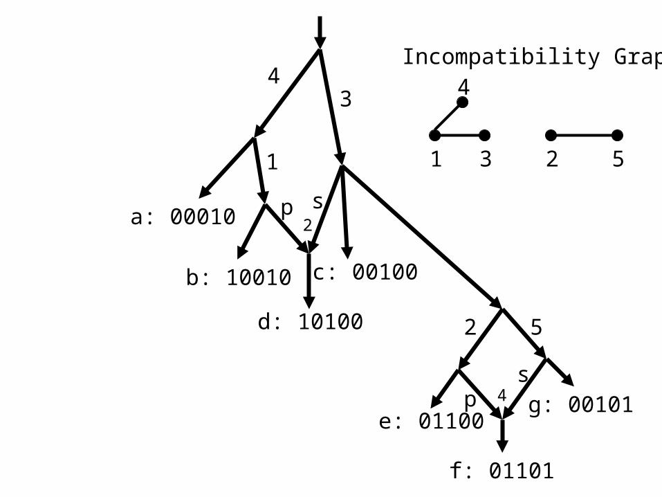
Very Simplistic Mapping the Unobserved Mutation of Mendelian Diseases with ARGs

Diseased

Assumption (for now): A sequence is diseased iff it carries the single disease mutation

Where is the disease mutation?

1 2 3 4 5

What part of 01100 d, e, f inherit?

d: e:f:

? ?

The single disease mutation occurs near sites 1 or 2!

Mapping Disease Gene with Inferred ARGs

• “..the best information that we could possibly get about association is to know the full coalescent genealogy…” – Zollner and Pritchard, 2005

• But we do not know the true ARG! • Goal: infer ARGs from SNP data for

association mapping– Not easy and often approximation (e.g. Zollner and

Pritchard)– Improved results to do Y. Wu (RECOMB 2007)

Results on Reconstructing the Evolution of SNP Sequences

• Part I: Clean mathematical and algorithmic results: Galled-Trees, near-uniqueness, graph-theory lower bound, and the Decomposition theorem

• Part II: Practical computation of Lower and Upper bounds on the number of recombinations needed. Construction of (optimal) phylogenetic networks; uniform sampling; haplotyping with ARGs

• Part III: Applications

• Part IV: Extension to Gene Conversion

Problem: If not a tree, then what?

If the set of sequences M cannot be derived on a perfect phylogeny (true tree) how much deviation from a tree is required?

We want a network for M that uses a small number of recombinations, and we want the resulting network to be as ``tree-like” as possible.

4

1

3

2 5

a: 00010

b: 10010

d: 10100

c: 00100

e: 01100

f: 01101

g: 00101

A tree-like networkfor the same sequences generatedby the prior network.

2

4

p s

ps

Recombination Cycles

• In a Phylogenetic Network, with a recombination node x, if we trace two paths backwards from x, then the paths will eventually meet.

• The cycle specified by those two paths is called a ``recombination cycle”.

Galled-Trees

• A phylogenetic network where no recombination cycles share an edge is called a galled tree.

• A cycle in a galled-tree is called a gall.

• Question: if M cannot be generated on a true tree, can it be generated on a galled-tree?

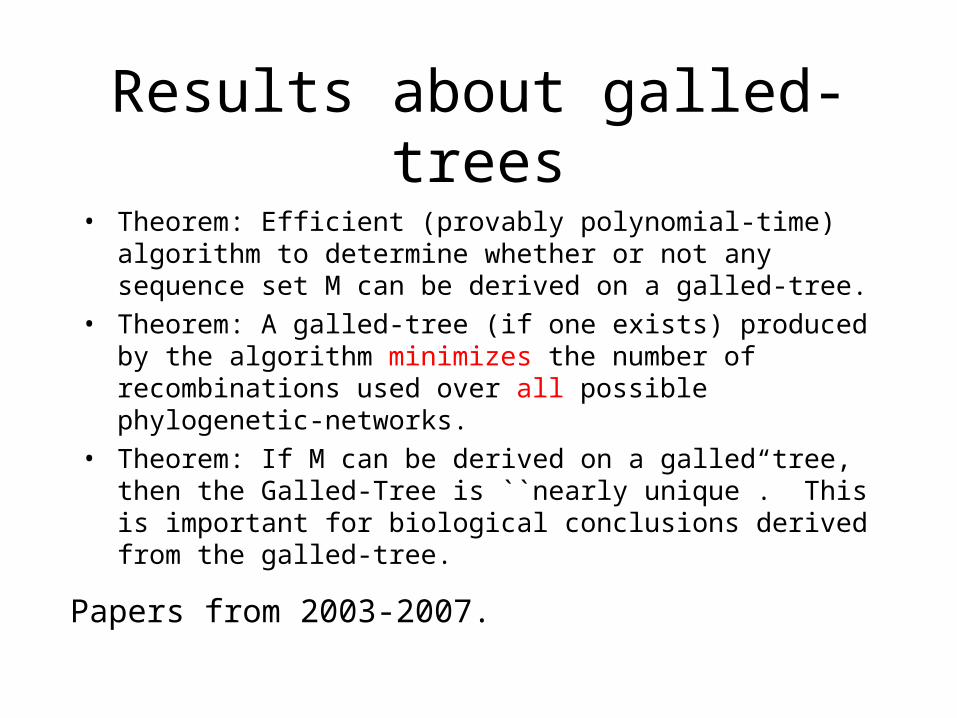
Results about galled-trees

• Theorem: Efficient (provably polynomial-time) algorithm to determine whether or not any sequence set M can be derived on a galled-tree.

• Theorem: A galled-tree (if one exists) produced by the algorithm minimizes the number of recombinations used over all possible phylogenetic-networks.

• Theorem: If M can be derived on a galled tree, then the Galled-Tree is ``nearly unique”. This is important for biological conclusions derived from the galled-tree.

Papers from 2003-2007.

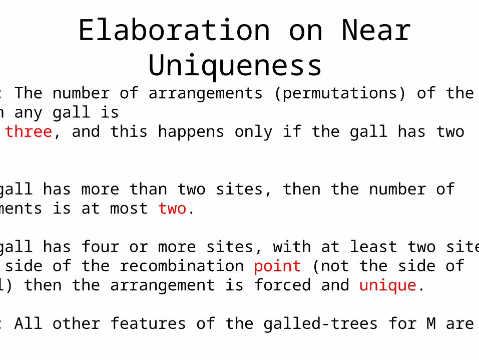
Elaboration on Near Uniqueness

Theorem: The number of arrangements (permutations) of the sites on any gall isat most three, and this happens only if the gall has two sites.

If the gall has more than two sites, then the number ofarrangements is at most two.

If the gall has four or more sites, with at least two siteson each side of the recombination point (not the side ofthe gall) then the arrangement is forced and unique.

Theorem: All other features of the galled-trees for M are invariant.

A whiff of the ideas behind the results

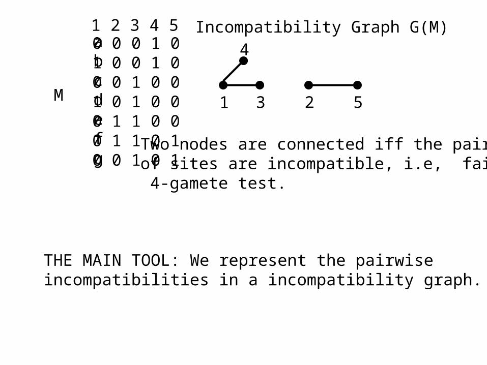
Incompatible Sites

A pair of sites (columns) of M that fail the

4-gametes test are said to be incompatible.

A site that is not in such a pair is compatible.

0 0 0 1 01 0 0 1 00 0 1 0 01 0 1 0 00 1 1 0 00 1 1 0 10 0 1 0 1

1 2 3 4 5abcdefg

1 3

4

2 5

Two nodes are connected iff the pairof sites are incompatible, i.e, fail the 4-gamete test.

Incompatibility Graph G(M)

M

THE MAIN TOOL: We represent the pairwise incompatibilities in a incompatibility graph.

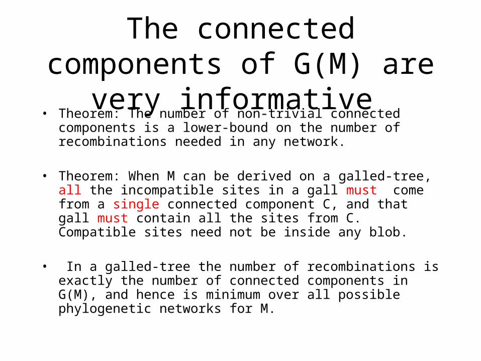
The connected components of G(M) are very informative

• Theorem: The number of non-trivial connected components is a lower-bound on the number of recombinations needed in any network.

• Theorem: When M can be derived on a galled-tree, all the incompatible sites in a gall must come from a single connected component C, and that gall must contain all the sites from C. Compatible sites need not be inside any blob.

• In a galled-tree the number of recombinations is exactly the number

of connected components in G(M), and hence is minimum over all possible phylogenetic networks for M.

4

1

3

2 5

a: 00010

b: 10010

d: 10100

c: 00100

e: 01100

f: 01101

g: 00101

2

4

p s

ps

1 3

4

2 5

Incompatibility Graph

Generalizing beyond Galled-Trees

When M cannot be generated on a true tree or a galled-tree, what then?

What role for the connected components of G(M) in general?

What is the most tree-like network for M?Can we minimize the number of

recombinations needed to generate M?

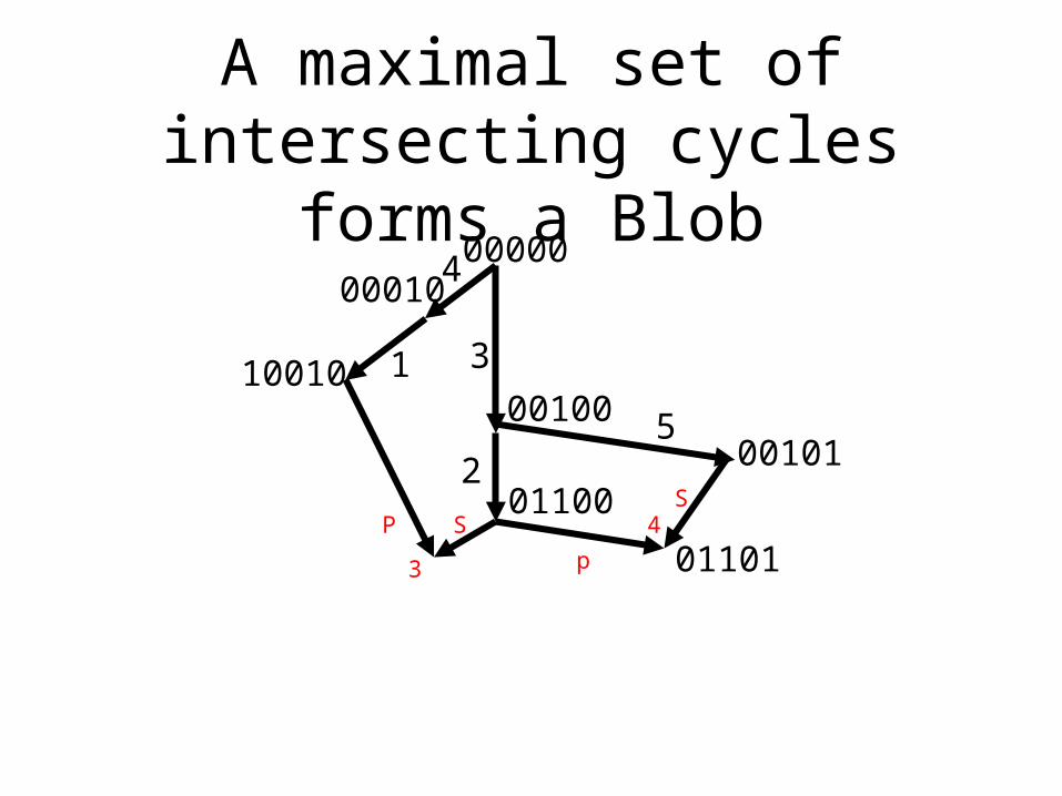
A maximal set of intersecting cycles forms a Blob

00000

52

3

3

4S

p

PS

1

4

10010

0110000101

01101

00100

00010

Blobs generalize Galls

• In any phylogenetic network a maximal set of intersecting cycles is called a blob. A blob with only one cycle is a gall.

• Contracting each blob results in a directed, rooted tree, otherwise one of the “blobs” was not maximal. Simple, but key insight.

• So every phylogenetic network can be viewed as a directed tree of blobs - a blobbed-tree.

The blobs are the non-tree-like parts of the network.

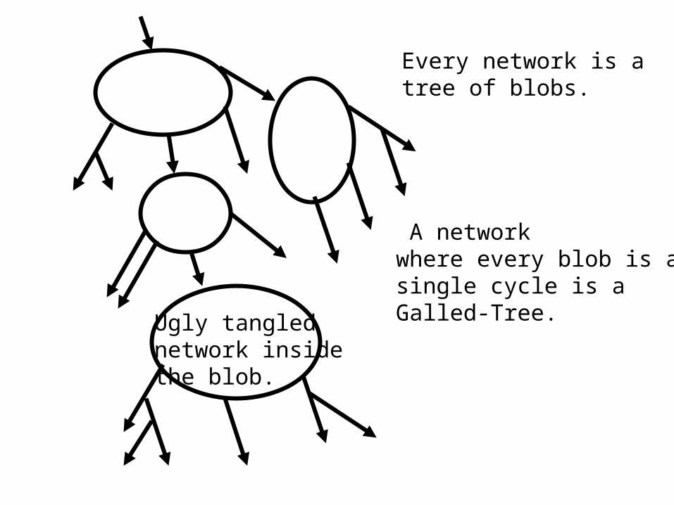
Ugly tanglednetwork insidethe blob.

Every network is a tree of blobs.

A network where every blob is a single cycle is a Galled-Tree.

The Decomposition Theorem

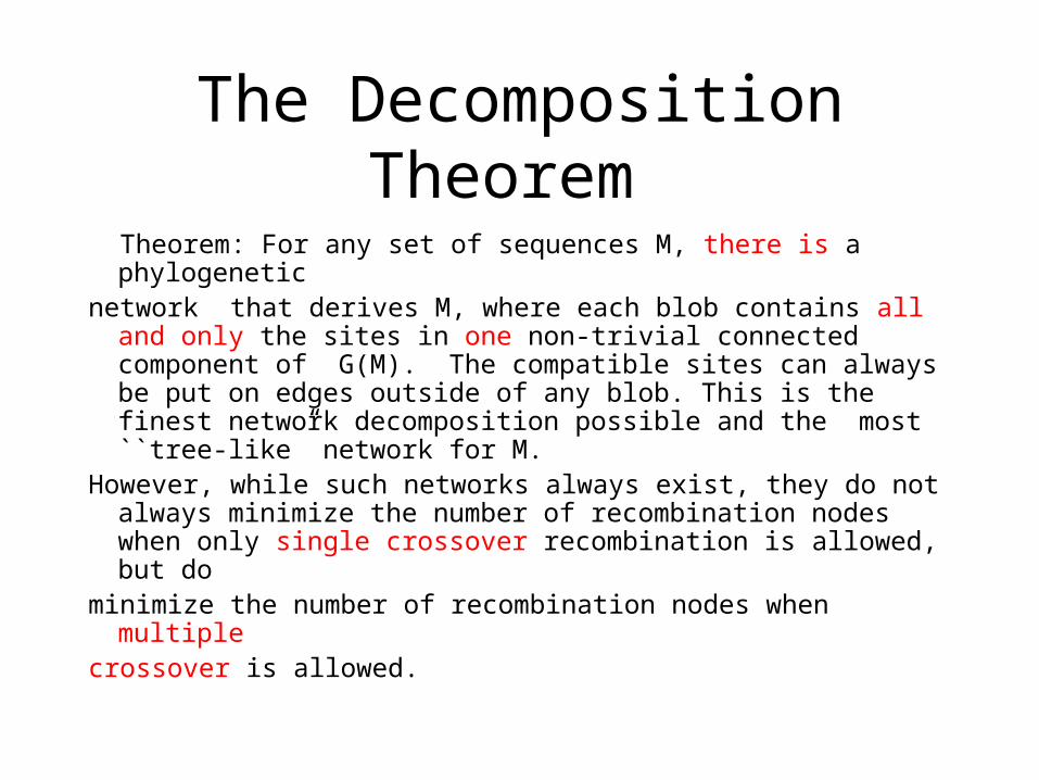
Theorem: For any set of sequences M, there is a phylogenetic network that derives M, where each blob contains all and only

the sites in one non-trivial connected component of G(M). The compatible sites can always be put on edges outside of any blob. This is the finest network decomposition possible and the most ``tree-like” network for M.

However, while such networks always exist, they do not always minimize the number of recombination nodes when only single crossover recombination is allowed, but do

minimize the number of recombination nodes when multiplecrossover is allowed.

Minimizing recombinations in unconstrained networks

• When a galled-tree exists it minimizes the number of recombinations used over all possible phylogenetic networks for M. But a galled-tree is not always possible.

• Problem: given a set of sequences M, find a phylogenetic network generating M, minimizing the number of recombinations used to generate M.

Minimization is an NP-hard Problem

There is no known efficient

solution to this problem and there likely will never be one.

What we do: Solve small data-sets optimally with algorithms that are not provably efficient but work well inpractice;

Efficiently compute lower and upper bounds on the number of needed recombinations.

Part II: Constructing optimal phylogenetic networks in general

Computing close lower and upper bounds on

the minimum number of recombinations needed to derive M. (ISMB 2005)

The grandfather of all lower bounds - HK 1985

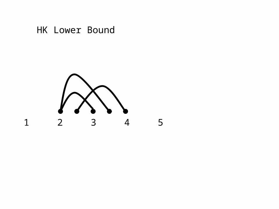
• Arrange the nodes of the incompatibility graph on the line in order that the sites appear in the sequence. This bound requires a linear order.

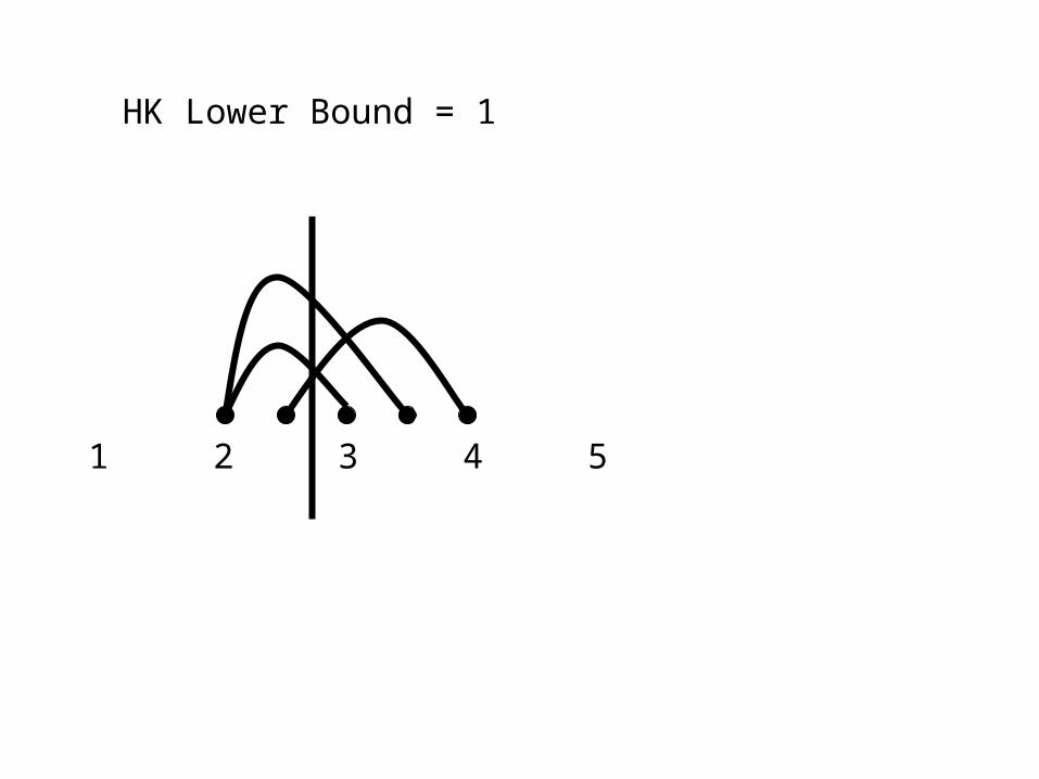
• The HK bound is the minimum number of vertical lines needed to cut every edge in the incompatibility graph. Weak bound, but widely used - not only to bound the number of recombinations, but also to suggest their locations.

Justification for HK

If two sites are incompatible, there must have been some recombination where the crossover point is between the two sites.

1 2 3 4 5

HK Lower Bound

1 2 3 4 5

HK Lower Bound = 1

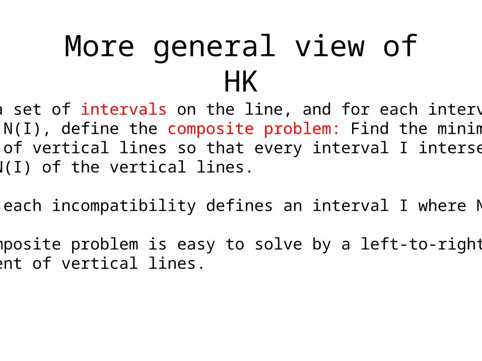
More general view of HK

Given a set of intervals on the line, and for each interval I, a number N(I), define the composite problem: Find the minimum number of vertical lines so that every interval I intersects at least N(I) of the vertical lines.

In HK, each incompatibility defines an interval I where N(I) = 1.

The composite problem is easy to solve by a left-to-right myopicplacement of vertical lines.

This general approach is called the Composite Method(Simon Myers 2002).

If each N(I) is a ``local” lower bound on the number ofrecombinations needed in interval I, then the solution tothe composite problem is a valid lower bound for thefull sequences. The resulting bound is called the compositebound given the local bounds.

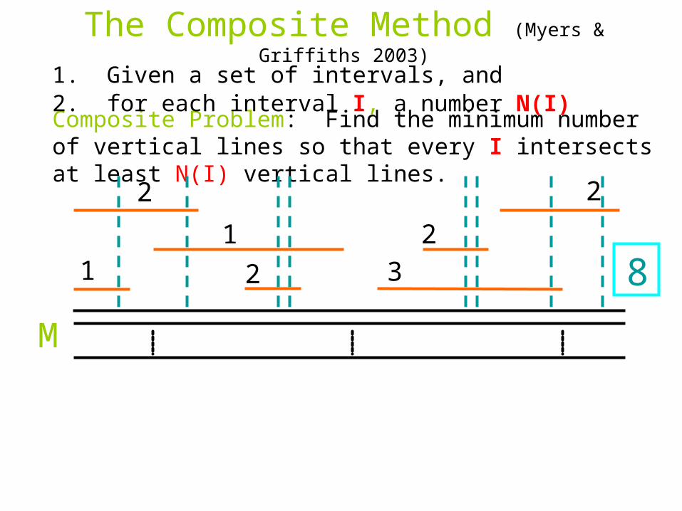
The Composite Method (Myers & Griffiths 2003)

M

1. Given a set of intervals, and

Composite Problem: Find the minimum number of vertical lines so that every I intersects at least N(I) vertical lines.

2

1

2

2

2

31

2. for each interval I, a number N(I)

8

Haplotype Bound (Simon Myers)

• Rh = Number of distinct sequences (rows) - Number of distinct sites (columns) -1 <= minimum number of recombinations needed (folklore)

• Before computing Rh, remove any site that is compatible with all other sites. A valid lower bound results - generally increases the bound.

• Generally Rh is really bad bound, often negative, when used on large intervals, but Very Good when used as local bounds in the Composite Interval Method, and other methods.

Composite Subset Method (Myers)

• Let S be subset of sites, and Rh(S) be the haplotype bound for subset S. If the leftmost site in S is L and the rightmost site in S is R, then use Rh(S) as a local bound N(I) for interval I = [S,L].

• Compute Rh(S) on many subsets, and then solve the composite problem to find a composite bound.

RecMin (Myers)

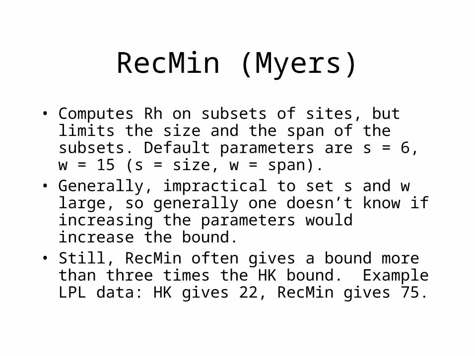
• Computes Rh on subsets of sites, but limits the size and the span of the subsets. Default parameters are s = 6, w = 15 (s = size, w = span).

• Generally, impractical to set s and w large, so generally one doesn’t know if increasing the parameters would increase the bound.

• Still, RecMin often gives a bound more than three times the HK bound. Example LPL data: HK gives 22, RecMin gives 75.

Optimal RecMin Bound (ORB)

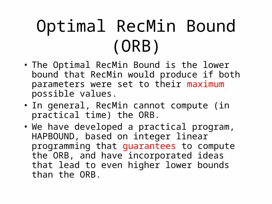
• The Optimal RecMin Bound is the lower bound that RecMin would produce if both parameters were set to their maximum possible values.

• In general, RecMin cannot compute (in practical time) the ORB.

• We have developed a practical program, HAPBOUND, based on integer linear programming that guarantees to compute the ORB, and have incorporated ideas that lead to even higher lower bounds than the ORB.

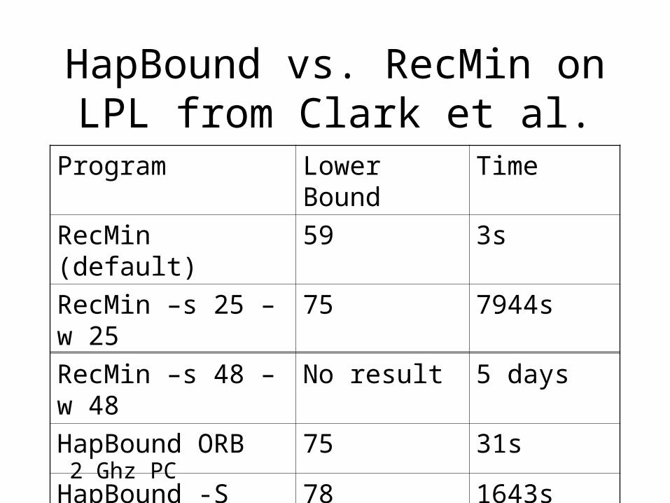
HapBound vs. RecMin on LPL from Clark et al.

Program Lower Bound Time

RecMin (default) 59 3s

RecMin –s 25 –w 25 75 7944s

RecMin –s 48 –w 48 No result 5 days

HapBound ORB 75 31s

HapBound -S 78 1643s

2 Ghz PC

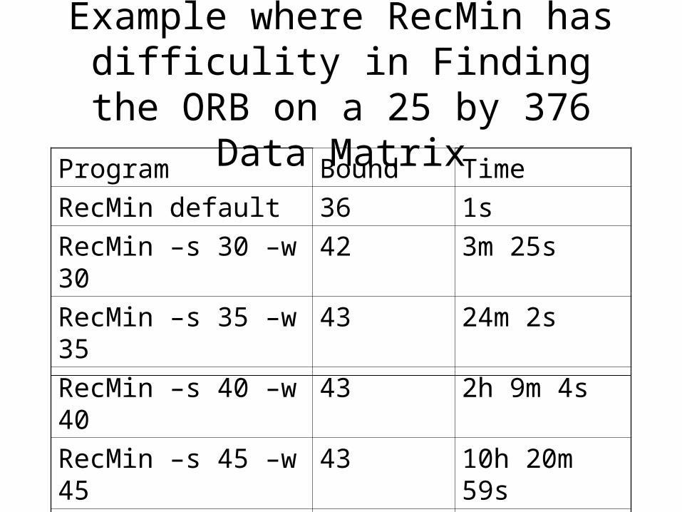
Example where RecMin has difficulity in Finding the ORB on a

25 by 376 Data MatrixProgram Bound Time

RecMin default 36 1s

RecMin –s 30 –w 30 42 3m 25s

RecMin –s 35 –w 35 43 24m 2s

RecMin –s 40 –w 40 43 2h 9m 4s

RecMin –s 45 –w 45 43 10h 20m 59s

HapBound 44 2m 59s

HapBound -S 48 39m 30s

Constructing Optimal Phylogenetic Networks in

General

Optimal = minimum number of recombinations. Called Min ARG.

The method is based on the coalescent

viewpoint of sequence evolution. We build

the network backwards in time.

Kreitman’s 1983 ADH Data

• 11 sequences, 43 segregating sites

• Both HapBound and SHRUB took only a fraction of a second to analyze this data.

• Both produced 7 for the number of detected recombination events

Therefore, independently of all other methods, our lower and upper bound methods together imply that 7 is the minimum number of recombination events.

A Min ARG for Kreitman’s data

QuickTime™ and aTIFF (LZW) decompressor

are needed to see this picture.

ARG created by SHRUB

The Human LPL Data (Nickerson et al. 1998)

QuickTime™ and aTIFF (LZW) decompressor

are needed to see this picture.

QuickTime™ and aTIFF (LZW) decompressor

are needed to see this picture.

Our new lower and upper bounds

Optimal RecMin Bounds

(We ignored insertion/deletion, unphased sites, and sites with missing data.)

(88 Sequences, 88 sites)

Part III: Applications

Uniform Sampling of Min ARGs

• Sampling of ARGs: useful in statistical applications, but thought to be very challenging computationally. How to sample uniformly over the set of Min ARGs?

• All-visible ARGs: A special type of ARG – Built with only the input sequences– An all-visible ARG is a Min ARG

• We have an O(2n) algorithm to sample uniformly from the all-visible ARGs.– Practical when the number of sites is small

• We have heuristics to sample Min ARGs when there is no all-visible ARG.

Application: Association Mapping

• Given case-control data M, uniformly sample the minimum ARGs (in practice for small windows of fixed number of SNPs)

• Build the ``marginal” tree for each interval between adjacent recombination points in the ARG

• Look for non-random clustering of cases in the tree; accumulate statistics over the trees to find the best mutation explaining the partition into cases and controls.

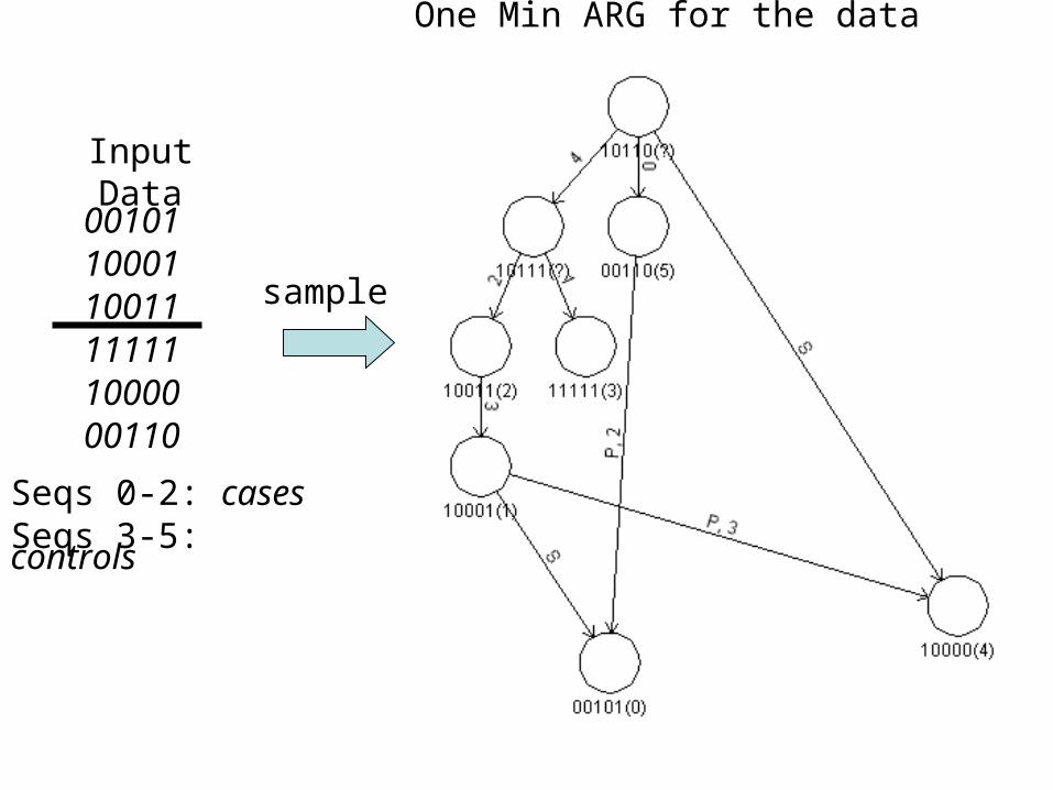
Input Data

001011000110011111111000000110

Seqs 0-2: casesSeqs 3-5: controls

sample

One Min ARG for the data

Input Data

001011000110011111111000000110

Seqs 0-2: casesSeqs 3-5: controls

Tree

The marginal tree for the interval past both breakpoints

Cases

Experimental results on Cystic Fibrosis data. Disease mutation is at 885kb. Our estimate is at

844kb.

0

10

20

30

40

50

60

70

80

0 5 10 15 20 25

Marker indices

Average Chi-square value

Haplotyping (Phasing)

genotypic data using a Min ARG

Minimizing Recombinations for Genotype Data

• Haplotyping (phasing genotypic data) via a Min ARG: attractive but difficult

• We have a branch and bound algorithm that builds a Min ARG for deduced haplotypes that generate the given genotypes. Works for genotype data with a small number of sites, but a larger number of genotypes.

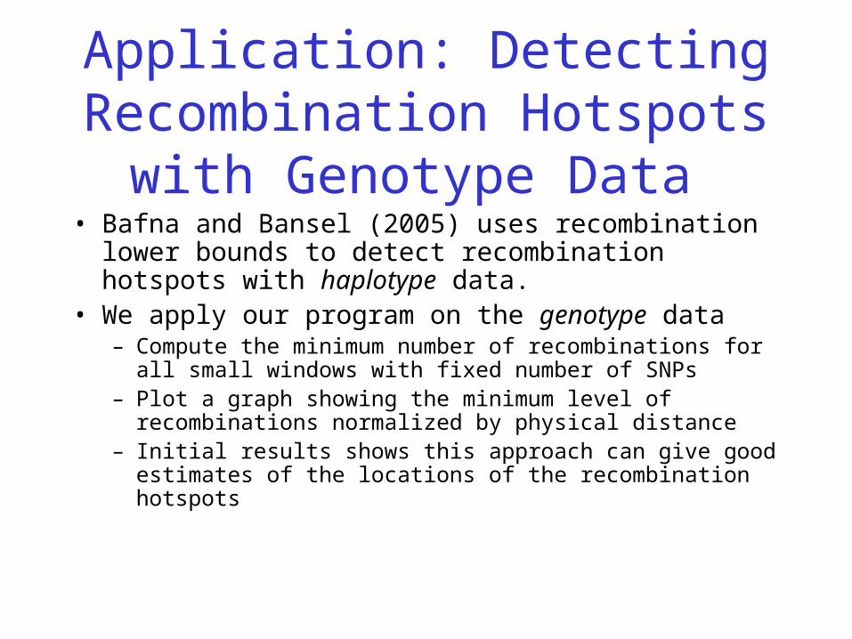
Application: Detecting Recombination Hotspots with

Genotype Data • Bafna and Bansel (2005) uses recombination lower

bounds to detect recombination hotspots with haplotype data.

• We apply our program on the genotype data– Compute the minimum number of recombinations for all

small windows with fixed number of SNPs– Plot a graph showing the minimum level of recombinations

normalized by physical distance– Initial results shows this approach can give good estimates

of the locations of the recombination hotspots

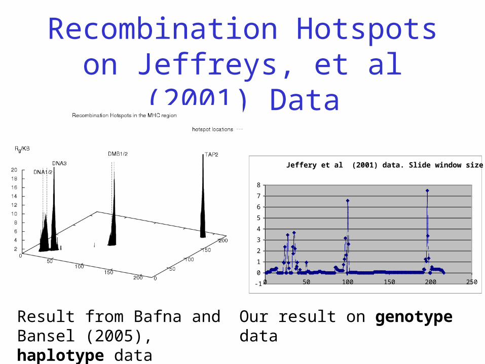
Recombination Hotspots on Jeffreys, et al (2001) Data

Jeffery et al (2001) data. Slide window size = 5

-1

0

1

2

3

4

5

6

7

8

0 50 100 150 200 250

Result from Bafna and Bansel (2005), haplotype data

Our result on genotype data

Haplotyping genotype data via a minimum ARG

• Compare to program PHASE, speed and accuracy: comparable for certain range of data

• Experience shows PHASE may give solutions whose recombination is close to the minimum– Example: In all solutions of PHASE for three sets of

case/control data from Steven Orzack, recombinatons are minimized.

– Simulation results: PHASE’s solution minimizes recombination in 57 of 100 data (20 rows and 5 sites).

Papers and Software on wwwcsif.cs.ucdavis.edu/~gusfield