Algorithms for the On-line Travelling Salesman �Giorgio Ausielloy Esteban Feuersteinz Stefano LeonardiyLeen Stougiex Maurizio TalamoyJuly 13, 1999AbstractIn this paper the problem of e�ciently serving a sequence of requests presentedin an on-line fashion located at points of a metric space is considered. We call thisproblem the On-Line Travelling Salesman Problem (OLTSP). It has a variety ofrelevant applications in logistics and robotics.We consider two versions of the problem. In the �rst one the server is notrequired to return to the departure point after all presented requests have beenserved. For this problem we derive a lower bound on the competitive ratio of 2 onthe real line. Besides, a 2:5-competitive algorithm for a wide class of metric spaces,and a 7=3-competitive algorithm for the real line are provided.For the other version of the problem, in which returning to the departure pointis required, we present an optimal 2-competitive algorithm for the above mentionedgeneral class of metric spaces. If in this case the metric space is the real line wepresent a 1:75-competitive algorithm that compares with a �1:64 lower bound.Keywords: on-line algorithms, competitive analysis, travelling salesman problem, vehiclerouting.�Part of the results of this paper have already appeared in the Proceedings of the 4th ScandinavianWorkshop on Algorithm Theory, LNCS 824, Springer-Verlag, 1994, and in the Proceedings of the 4thInternational Workshop on Algorithms and Data Structures, LNCS 955, Springer-Verlag, 1995.yDipartimento di Informatica e Sistemistica, Universit�a di Roma \La Sapienza", via Salaria 113, 00198-Roma, Italia. This work was partly supported by EU ESPRIT Long Term Research Project ALCOM-ITunder contract No.20244, and by the Italian Ministry of Scienti�c Research, Project 40% \E�cienza diAlgoritmi e Progetto di Strutture Informative". e-mail: fausiello,leon,talamog@dis.uniroma1.itzDepartamento de Computaci�on, Facultad de Ciencias Exactas y Naturales, Universidad de BuenosAires and Instituto de Ciencias, Universidad de General Sarmiento, Argentina. Partly supported bythe KIT program of the European Community under contract n. 131 (DYNDATA) and by UBA's\Programaci�on para Investigadores J�ovenes" project \Algoritmos e�cientes para problemas on-line conaplicaciones". e-mail: esteban@dc.uba.arxDepartment of Mathematics, Eindhoven University of Technology, PO Box 513, 5600MB Eindhoven,The Netherlands. Supported by the Human Capital Mobility Network DONET of the European Com-munity. e-mail: leen@win.tue.nl

1 IntroductionThe Travelling Salesman Problem (TSP) and in general vehicle routing and schedulingproblems have been widely studied for more than three decades (see [14] for a surveyon the subject). The input of an instance of the problem is generally a set of locations(points) in a metric space that are to be visited in such a way that the total distancetravelled or the completion time is minimized. A common characteristic of almost all theapproaches to the study of the problem is the o�-line point of view. The input is knowncompletely beforehand.However, in many routing and scheduling applications the instance becomes onlyknown in an on-line fashion. In other words, the input of the problem is communi-cated in successive steps. Often it is even not possible to determine which is the lastrequest, i.e. when the instance is completely known. Anyhow, if the goal is to minimizethe completion time, waiting till all the information is available could imply a costly lossof time.In this paper we consider a class of on-line variations of TSP in a metric space: whilethe salesman is travelling, new sites to visit may be communicated to him. His goal is tovisit all the sites, minimizing the completion time.This setting models many natural applications. Think for example of a salesman or arepairman with a cellular phone, or of a robot that has to serve locations of its workingspace (for example in the Euclidean plane) and of many other routing and schedulingproblems on a transportation network modeled with a graph. We will refer to this problemas the On-line Travelling Salesman Problem (OLTSP).As the input to the salesman { from now on we will refer to him as the server { iscommunicated in an on-line way, the scheduled route will have to be updated also in anon-line way during the trip. The fact that the schedule must be constructed based onincomplete information means that in general no algorithm (polynomial or otherwise) canbe guaranteed to construct an optimal schedule on-line.The most widely accepted way of measuring the performance of on-line algorithms iscompetitive analysis. The quality of a certain on-line strategy is measured by the worst-case ratio between the time needed by the on-line algorithm for a sequence of requestsand the optimal time needed by an algorithm that knows the sequence in advance. Thisratio is called the competitive ratio of the on-line algorithm. Therefore, an algorithmis said to be �-competitive if for every input its completion time is at most � times theoptimal completion time for the same input. The concept of competitive analysis has been1

formalized in [18], although under the name of worst-case analysis of on-line algorithmsit dates back at least until the work of Graham [10] and Johnson [11]. The performanceof on-line strategies for a great variety of on-line problems has been analyzed accordingto this concept: performance analysis of computer systems, data structures, scheduling,motion planning, network management, �nancial decision making, etc. (for an overviewof the subject we refer to [3]).We present algorithms for the OLTSP and study their competitive ratio by comparingtheir performance to the optimal solution of the corresponding o�-line problem, which iscalled the Vehicle Routing Problem with release times [16].In that problem, each site must be visited at or after a given release time. The releasetime of a request corresponds to the time in which the request is communicated to theon-line server. The problem is NP-hard since it contains the Hamiltonian Path problemas a particular case.Several o�-line variations of the problem have been studied, in which additional con-straints are imposed and particular metric spaces are considered. In [16] it has been shownthat if the metric space is a line the optimal solution may be found in quadratic time.In [12] the metric space is restricted to be a tree and each request has, besides a releasetime, an associated handling time that is the time needed to serve it. The problem isshown to be NP-hard in that context, and a 2-approximate solution is given. In generalthese problems are called routing and scheduling with time window constraints. Some-times more than one server is considered, and other restrictions are given by requiringthat requests must be served before a speci�ed deadline (see for example [20, 21]). Otherrelated works are [2, 6, 7, 8].A related on-line work [13] considers the problem of visiting the whole set of verticesof an unknown graph, when the set of edges leaving a node is revealed only once the nodeis visited. In our case, the metric space is completely known from the beginning, butwhat is revealed in an on-line way is the set of locations that must be visited.It is important to note that OLTSP is di�erent from the famous k-server problem [15].In that problem the requests have to be served in the order in which they are presented,with the goal of minimizing the total distance travelled by the k servers. On the contrary,in OLTSP the task is precisely to decide the order in which the requests will be served.A recent paper [1] considers a �xed number of clients presenting sequences of requestsin a metric space, that must be served by a single server. At any time, each client hasat most one request to be served, after which a new one may be presented. The main2

di�erence with our approach is that, in this case the request sequence is dependent onthe behaviour of the algorithm.We consider two versions of the basic problem that requires that all points presentedare visited. In the �rst version, that we call Nomadic-OLTSP (or simply N-OLTSP) thisis the only requirement. Adding the constraint that the trip must end at its departurepoint de�nes the problem that we call Homing-OLTSP (or simply H-OLTSP).Addition of the constraint of ending the trip at the departure point changes the natureof the problem (and hence the kind of applications). Lower bounds and algorithms forthe two versions are quantitatively and qualitatively di�erent. In fact, knowing that theserver has to return to the departure point provides additional information to the on-linealgorithm, that allows it to achieve a better competitive ratio.In this work we propose on-line deterministic algorithms for both N-OLTSP and H-OLTSP, and show that they are �-competitive for suitable constants �. We establish suchresults for the problems de�ned on a wide class of metric spaces that we call the classM,whose precise de�nition can be found at the beginning of the following section. In theparticular case in which the metric space is the real line di�erent algorithms are devisedand stronger ratios of competitiveness are derived.For N-OLTSP, no on-line algorithm can be better than 2-competitive, even for theline. For metric spaces belonging to the classM we propose a 2:5-competitive algorithm;for the line the best proposed algorithm has competitive ratio 7=3.For H-OLTSP we propose a best possible 2-competitive algorithm for metric spacesbelonging to the class M, while for the line we devise a 1:75-competitive algorithm thatcompares with a � 1:64 lower bound.Our best algorithms for metric spaces belonging toM do not run in polynomial timeunless P=NP, since they use subroutines for optimally solving the TSP. However, one canobtain almost as good performance from polynomial-time algorithms: we show how toobtain 3-competitive polynomial-time algorithms for both N-OLTSP and H-OLTSP. As wementioned before, the on-line nature of the problem is a source of di�culty independent ofits computational complexity, and therefore on-line algorithms achieving good competitiveratios are of interest also if their time requirements are not polynomially bounded.The paper is organized as follows. In Section 2 we formally de�ne the model. InSection 3 we present our lower bounds for the di�erent versions of the problem. Section4 contains our best algorithms for metric spaces belonging to M, while Section 5 dealswith polynomial time algorithms. Section 6 proposes algorithms for the real line. To3

facilitate the exposition, every section �rst describes results on N-OLTSP and afterwardsfor H-OLTSP. Finally Section 7 contains open problems and interesting related problemsfor future research.2 The modelThe input of OLTSP consists of a metric space M , from the class M de�ned below, adistinguished point o (the origin) of M , and a sequence of pairs < ti; pi > where pi is apoint of M and ti is a number representing the moment in which the request is presented.The ti's form an ordered sequence in the sense that 0 � ti � tj if i < j.A server is located at the origin o of the metric space at time 0, and moves not fasterthan unit speed.We use the de�nition of metric space as a space M with the following properties: (1)It is symmetric, i.e., for every pair of points x; y in M , d(x; y) = d(y; x), where d(x; y)denotes the distance from x to y; (2) d(x; x) = 0 for any point x in M ; (3) It satis�es thetriangle inequality, i.e., for any triple of points x; y, and z inM , d(x; y) � d(x; z)+d(z; y).Our class of metric spaces M contains all continuous metric spaces, i.e., every metricspace M having the property that the shortest path from x 2M to y 2M is continuous,formed by points in M , and has length d(x; y). For continuous metric spaces the timesat which a request can be made can be any non-negative real number.NextM contains discrete metric spaces representable by an underlying graph with alledges having unit length. The vertices are the points of the metric space. Working onsuch spaces time needs to be discretized, i.e., the times ti at which requests are made arenon-negative integers, and the server determines its strategy at integer points in time. Ateach integer time, the server is at some point in the metric space (vertex in the graph)and either remains there or moves in one time step to a neighboring point in the metricspace.Thus, an example of a model that we do not consider here is one in which the servermoves on a road network of freeways and a request can arrive while he is moving betweentwo exits and he has to proceed to the next exit before being able to change his strategy.In our model the server would be allowed to do a U-turn and return to the previous exit.For any path T in M , let jT j denote its length. Note that if T is a path from x to y,we must have jT j � d(x; y) by the triangle inequality.As mentioned in the Introduction we consider two versions of the problem:4

The Nomadic On-line Travelling Salesman Problem - (N-OLTSP), de�ned as mini-mizing the completion time required to serve all presented requests;The Homing On-line Travelling Salesman Problem - (H-OLTSP), de�ned as minimiz-ing the completion time required to serve all presented requests and return to the origino. On-line algorithms for the problems N-OLTSP and H-OLTSP determine the behaviorof the server at a certain moment t as a function of all requests < ti; pi > such that ti � t.We will denote the completion time of the solution produced by an on-line algorithmOL by ZOL and that of the optimal (o�-line) solution by Z�. An on-line algorithm forOLTSP is �-competitive if for any sequence of requests ZOL � �Z�. Let pOL(t) and p�(t)respectively denote the positions of OL's server and the optimal o�-line server at time t.At time 0 the server is located at the origin o, pOL(0) = p�(0) = o.3 Lower boundsIn this section we derive lower bounds on the competitive ratio of any on-line strategy forserving the requests in the versions of the problem.3.1 A lower bound for N-OLTSPWe show that no on-line algorithm can achieve a competitive ratio smaller than 2 forN-OLTSP. With this aim, we provide a sequence of requests for which no algorithm can�nish within less than twice the optimal o�-line time.Theorem 3.1 Any �-competitive algorithm for N-OLTSP has � � 2. The lower boundis achieved on the real line.Proof: The proof is derived from the following simple argument. Consider the prob-lem on the real line with the abscissa 0 as the origin. An adversary gives a request at time1 in either 1 or -1, depending on whether at time 1 the on-line server is in a negative or apositive position, respectively. Thus, the adversary has completed at time 1, whereas theon-line server needs at least 2, with 2 su�cing when it is at 0 at time 1. 2We observe that the former proof can be easily adapted to show that the same lowerbound holds for randomized algorithms against an oblivious adversary. The same simplesequence can be used replacing the \position" of the on-line server by \expected position".For the de�nition of oblivious adversary we refer to [4].5

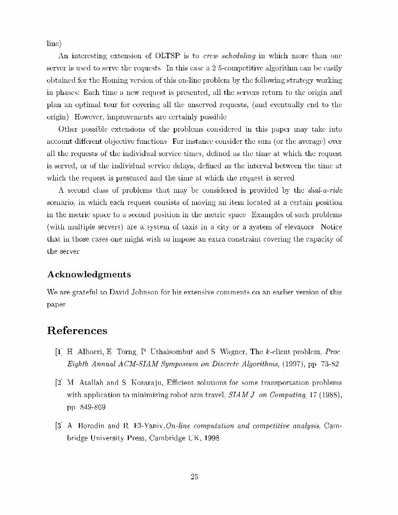
3.2 A lower bound for H-OLTSPIn this section we show a lower bound on the competitive ratio of any algorithm forH-OLTSP on metric spaces belonging to M.Theorem 3.2 For any � > 0, any �-competitive algorithm for H-OLTSP for metric spacesbelonging to M has � � 2� �.Proof: Take as the metric space the boundary of the unit square [0; 1]2. We denote by(x; y) a point of abscissa x and ordinate y. Given two points of the square (x1; y1) and(x2; y2), we denote by [(x1; y1); (x2; y2)] the segment that is obtained by traversing thesquare in clockwise direction from (x1; y1) to (x2; y2). The distance between two points isde�ned as the length of the shorter of the two segments of the boundary of the unit squarebetween the two points. As the origin we take the point (0; 0). At time 0, for a �xedn � 1, requests are given at points of the square f(0; i=n); i = 0; : : : ; ng [ f(1; i=n); i =0; : : : ; ng [ f(i=n; 0); i = 1; : : : ; n � 1g [ f(i=n; 1); i = 1; : : : ; n � 1g. Thus (0; 0), (1; 0),(0; 1) and (1; 1) belong to this set of points. Notice that these requests can be servedoptimally in time Z� = 4.We �rst show that for some �, with 0 � � � 2, at time 2 + � any on-line server mustbe in one of the two points at distance 2 � � from the origin (not necessarily requestedpoints). For this purpose de�ne the function f : [0; 2] ! [0; 2] as the distance from thepoint (1; 1) at time 2 + x. Then the function g(x) = f(x) � x has the property thatg(0) � 0 and g(2) � 0. Since g is continuous there must be at least one point � with0 � � � 2 with g(�) = 0.Take the smallest value of � for which this holds. Without loss of generality we assumethat this point pOL(2+�) is on the path between (0; 0) and (1; 1) that passes through (0; 1).At time 2 + � the server has served the requests on the segment T1 = [(0; 0); pOL(2 + �)].Additionally, it may have visited requests on a segment S1 = [(x1; y1); (0; 0)] and requestson a segment S2 = [pOL(2 + �); (x2; y2)] (see Figure 1). The total length of these lattertwo segments is no more than � since the server is at a distance 2� � from the origin andmust have travelled each of these segments at least twice. Thus, jT1j + jS1j + jS2j � 2This implies that the on-line algorithm has not touched any requested point of a segmentT2 = [(x2; y2); (x1; 0)] of length at least 2.Now, at time 2+ �, a new set of requests is given in each of the points on the segmentT1 = [(0; 0); pOL(2 + �)] of length 2 � �, that were requested before and visited by theon-line server. This new set of requests ends the sequence. The optimal completion time6

for the whole sequence is still Z� = 4 since an anti-clockwise tour of the square visits anyrequest not earlier than its release time. Given the situation of the on-line server at time2 + � one of the two following options will give the best possible completion time:1. Traverse twice the segment [pOL(2 + �); (x1; y1)] with the exception of a segment[(x1; y1); (x3; y3)] of size at most 1=n. The traversed segment is therefore of size atleast 2� 1=n. After this traverse once the segment T1. The cost of the algorithm isin this case ZOL � (2 + �) + (4� 2=n) + (2� �) = 8� 2=n.2. Traverse �rst twice the segment T1[(0; 0); (0; 1=n)] and then once the segment [pOL(2+�); (0; 0)]. The cost of the algorithm is in this case ZOL = (2+ �)+ (4� 2�� 2=n)+(2 + �) = 8� 2=n.Therefore, for any arbitrarily small � > 0, the ratio between the on-line server's com-pletion time and the optimal completion time can be made 2� � by choosing a su�cientlylarge value for n. 2We emphasize that this theorem says that some metric spaces in M can induce anyalgorithm for H-OLTSP to be no less than 2-competitive. Therefore, better competitiveratios may be possible for particular metric spaces, for instance for the line, as we shallsee in what follows.3.3 A lower bound for H-OLTSP on the lineIn this subsection we present a lower bound on the competitive ratio of algorithms forH-OLTSP de�ned on the real line. We study this case separately so as to compare thelower bound with the competitive ratio of an algorithm for the problem on the real linepresented in Section 6.2.An argument similar to that used for the lower bound for N-OLTSP (Theorem 3.1)could be used to obtain a 3/2 lower bound for H-OLTSP, both for deterministic andrandomized algorithms. However, a stronger lower bound for deterministic algorithms isproved below.Theorem 3.3 Any �-competitive algorithm for H-OLTSP on the real line has� � (9 +p17)=8 � 1:64. 7

Proof: Suppose OL is a �-competitive on-line algorithm for H-OLTSP with � < (9 +p17)=8. An adversary could proceed as follows. Before time t = 1 no requests arepresented. At that moment, the position pOL(1) of the server of the �-competitive on-linealgorithm OL must be inside the interval [�(2�� 3); (2�� 3)], and note that 2�� 3 < 1since � < 2. notice that if pOL(1) > (2��3) the �rst (and unique) request of the sequencewould be at point -1, giving ZOL > 1 + (2�� 3) + 2 = 2�, because OL has to travel fromits current position to -1 and back to 0. On the other hand, for this sequence Z� = 2, andtherefore the algorithm would not be �-competitive. The case in which pOL(1) < �(2��3)is symmetric.Thus, suppose that pOL(1) 2 [�(2�� 3); (2�� 3)]. Now, at time t = 1, the adversarypresents two simultaneous requests at points -1 and 1. At time t = 3, the on-line servercannot have served both requests. Suppose, without loss of generality, that it has notserved the request in -1.We now show that if �(7�4�) < pOL(3) < (7�4�), then OL can not be �-competitive.Note that 7 � 4� < 1 since � < 7=4. In this case the adversary could be in p�(3) = 1,present a new request in +1 and return to the origin with a completion time Z� = 4.OL, however, would still have to serve requests in both extremes, and hence ZOL >3 + 1� (7� 4�) + 3 = 4�, since starting at time t = 3 it would have to go to one of theextremes and then to the other and back to 0.Note that since � < (9+p17)=8, we have that the interval [�(7�4�); (7�4�)] strictlycontains the interval [�(2�� 3); (2�� 3)].Thus, we are left with two cases to be considered.1. At time t = 3 the on-line server has not yet served +1, and �1 � pOL(3) � �(7�4�)or (7� 4�) � pOL(3) � 1.2. At time t = 3 the on-line server has served +1, and (7 � 4�) � pOL(3) � 1. Theserver cannot be to the left of�(7�4�), since it started to move toward +1 after time1 from a position not to the right of (2��3), and 1+(1�(2��3))+(1+(2��3)) = 3.We notice that in both cases the following situation occurs: the on-line server is withindistance 1 � (7 � 4�) of the extreme on one side and has not served the extreme on theother side. This property is su�cient for the rest of the proof, where we will supposethat the on-line server is near 1 and has not served the request in -1 (the other case issymmetric). 8

In this case the adversary has so far served -1, is at position p�(3) = +1 and �nisheswith Z� = 4. Then, any �-competitive on-line algorithm has to pass point 0 no later than4� � 2. Let us denote the time at which the on-line server crosses the origin as 3 + q.Therefore we have q � 4�� 5 (1)At time (3 + q) the adversary can be in position (1 + q) and place a request at thatpoint and return to 0. For this sequence we have that ZOL = 7 + 3q and Z� = 4 + 2q,and therefore ZOLZ� = 7+3q4+2q . By hypothesis OL is �-competitive, so that� � 7 + 3q4 + 2qThis is a monotonously decreasing function of q, and by inequality (1) we get� � 7 + 3(4�� 5)4 + 2(4�� 5) (2)The least value of � that satis�es inequality (2) is the value that achieves equality,that is � = 9+p178 . 24 Algorithms for metric spaces in MIn this section we will present competitive algorithms for metric spaces belonging to M.The �rst algorithm we will analyze is based on a greedy strategy. Essentially it follows ateach time the shortest route that serves all the requests with, for H-OLTSP, the additionalconstraint of terminating at the origin of the metric space. For H-OLTSP we will alsopresent a more complicated algorithm that attains the best possible competitive ratio byfollowing di�erent rules for requests \close" to the origin and for requests \far" from theorigin. The reason is that requests close to the origin can be served when the server ison the way back to the origin, the endpoint of his route. Clearly, these considerations donot hold for N-OLTSP, where the server can end his work in any position of the metricspace.The above mentioned strategies use super polynomial time, assuming that P6=NP, sincethey need to compute an optimal path or an optimal tour over a set of points. We will alsopresent polynomial-time strategies (see Section 5) with worse competitive ratios, basedon polynomial approximation algorithms to compute a path or a tour over a set of points.9

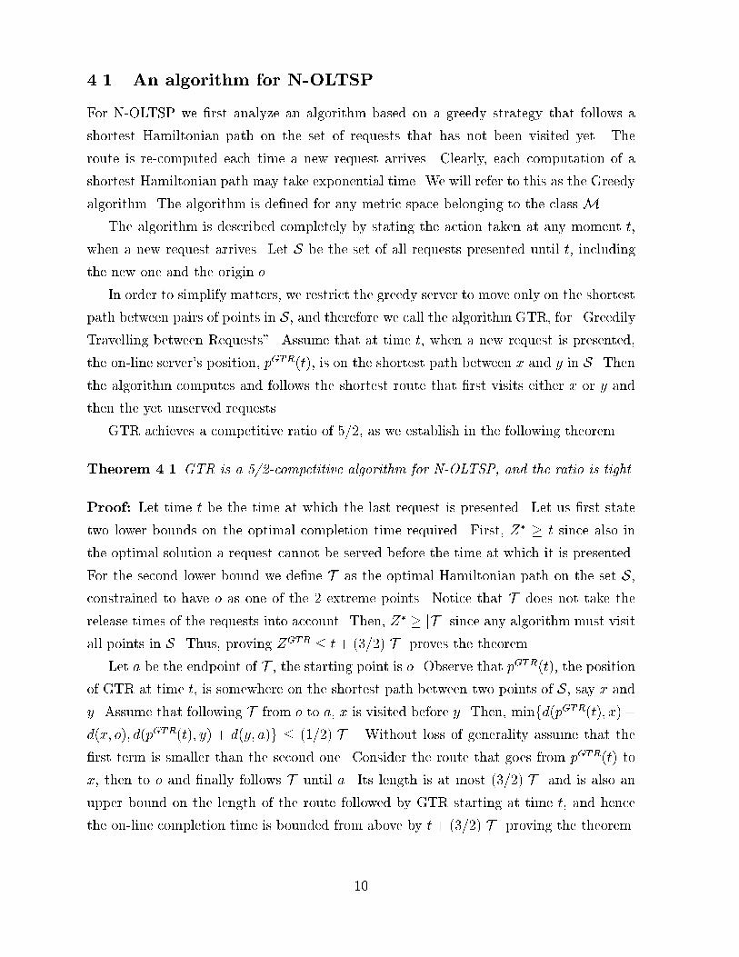
4.1 An algorithm for N-OLTSPFor N-OLTSP we �rst analyze an algorithm based on a greedy strategy that follows ashortest Hamiltonian path on the set of requests that has not been visited yet. Theroute is re-computed each time a new request arrives. Clearly, each computation of ashortest Hamiltonian path may take exponential time. We will refer to this as the Greedyalgorithm. The algorithm is de�ned for any metric space belonging to the class M.The algorithm is described completely by stating the action taken at any moment t,when a new request arrives. Let S be the set of all requests presented until t, includingthe new one and the origin o.In order to simplify matters, we restrict the greedy server to move only on the shortestpath between pairs of points in S, and therefore we call the algorithm GTR, for \GreedilyTravelling between Requests". Assume that at time t, when a new request is presented,the on-line server's position, pGTR(t), is on the shortest path between x and y in S. Thenthe algorithm computes and follows the shortest route that �rst visits either x or y andthen the yet unserved requests.GTR achieves a competitive ratio of 5=2, as we establish in the following theorem.Theorem 4.1 GTR is a 5/2-competitive algorithm for N-OLTSP, and the ratio is tight.Proof: Let time t be the time at which the last request is presented. Let us �rst statetwo lower bounds on the optimal completion time required. First, Z� � t since also inthe optimal solution a request cannot be served before the time at which it is presented.For the second lower bound we de�ne T as the optimal Hamiltonian path on the set S,constrained to have o as one of the 2 extreme points. Notice that T does not take therelease times of the requests into account. Then, Z� � jT j since any algorithm must visitall points in S. Thus, proving ZGTR � t+ (3=2)jT j proves the theorem.Let a be the endpoint of T , the starting point is o. Observe that pGTR(t), the positionof GTR at time t, is somewhere on the shortest path between two points of S, say x andy. Assume that following T from o to a, x is visited before y. Then, minfd(pGTR(t); x) +d(x; o); d(pGTR(t); y) + d(y; a)g � (1=2)jT j. Without loss of generality assume that the�rst term is smaller than the second one. Consider the route that goes from pGTR(t) tox, then to o and �nally follows T until a. Its length is at most (3=2)jT j and is also anupper bound on the length of the route followed by GTR starting at time t, and hencethe on-line completion time is bounded from above by t+ (3=2)jT j proving the theorem.10

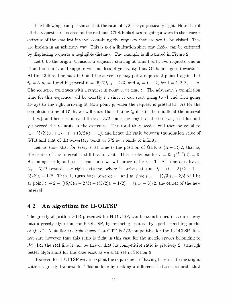
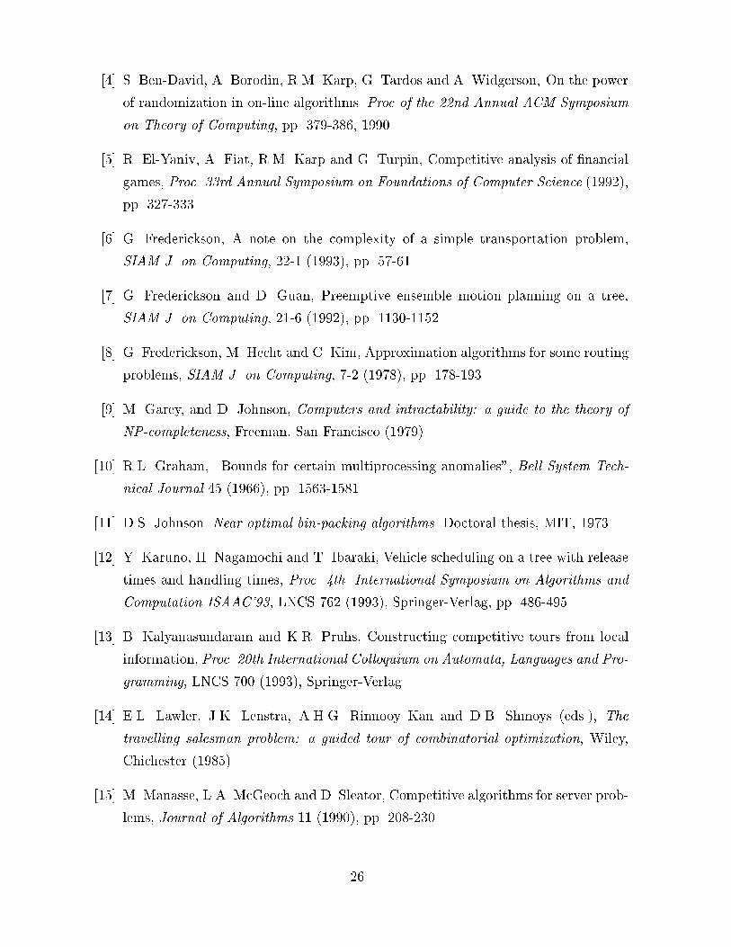
The following example shows that the ratio of 5/2 is asymptotically tight. Note that ifall the requests are located on the real line, GTR boils down to going always to the nearestextreme of the smallest interval containing the requests that are yet to be visited. Tiesare broken in an arbitrary way. This is not a limitation since any choice can be enforcedby displacing requests a negligible distance. The example is illustrated in Figure 2.Let 0 be the origin. Consider a sequence starting at time 1 with two requests, one in-1 and one in 1, and suppose without loss of generality that GTR �rst goes towards 1.At time 3 it will be back in 0 and the adversary may put a request at point 1 again. Lett0 = 3; p0 = 1 and in general ti = (5=3)ti�1 � 2=3, and pi = ti � 2, for i = 1; 2; 3; : : : ; n.The sequence continues with a request in point pi at time ti. The adversary's completiontime for this sequence will be exactly tn, since it can start going to -1 and then goingalways to the right arriving at each point pi when the request is presented. As for thecompletion time of GTR, we will show that at time tn it is in the middle of the interval[�1; pn], and hence it must still travel 3/2 times the length of the interval, as it has notyet served the requests in the extremes. The total time needed will then be equal totn + (3=2)(pn+ 1) = tn + (3=2)(tn� 1), and hence the ratio between the solution value ofGTR and that of the adversary tends to 5=2 as n tends to in�nity.Let us show that for every i, at time ti the position of GTR is (ti � 3)=2, that is,the center of the interval it still has to visit. This is obvious for i = 0: pGTR(3) = 0.Assuming the hypothesis is true for i we will prove it for i + 1. At time ti it leaves(ti � 3)=2 towards the right extreme, where it arrives at time ti + (ti � 3)=2 + 1 =(3=2)ti � 1=2. Then, it turns back towards -1, and at time ti+1 = (5=3)ti � 2=3 will beat point ti � 2� [((5=3)ti � 2=3)� ((3=2)ti � 1=2)] = (ti+1 � 3)=2, the center of the newinterval. 24.2 An algorithm for H-OLTSPThe greedy algorithm GTR presented for N-OLTSP, can be transformed in a direct wayinto a greedy algorithm for H-OLTSP, by replacing \paths" by \paths �nishing in theorigin o". A similar analysis shows that GTR is 5/2-competitive for the H-OLTSP. It isnot sure however that this ratio is tight in this case for the metric spaces belonging toM. For the real line it can be shown that its competitive ratio is precisely 2, althoughbetter algorithms for this case exist as we shall see in Section 6.However, for H-OLTSP we can exploit the requirement of having to return to the origin,within a greedy framework. This is done by making a di�erence between requests that11

are relatively close and those that are relatively far from the origin, where we postponeserving the former set of requests. The algorithm that we devise, and which we call PAH(for Plan-At-Home) achieves a competitive ratio of 2 for any metric space belonging toM. We emphasize that this is equal to the lower bound derived in Section 3.2. Weabbreviate the position pPAH(t) of the PAH algorithm by p.1. Whenever the server is at the origin, it starts to follow an optimal route that servesall the requests yet to be served and goes back to the origin.2. If at time t a new request is presented at point x, then it takes one of two actionsdepending on its current position p:2a. If d(x; o) > d(p; o), then the server goes back to the origin (following theshortest path from p) where it appears in a Case 1 situation.2b. If d(x; o) � d(p; o) then the server ignores it until it arrives at the origin, whereagain it reenters Case 1.Notice that requests that are presented between an occurrence of Case 2a and thearrival at the origin will not make the server deviate from his current shortest path backto the origin.Theorem 4.2 PAH is 2-competitive.Proof: Let t be the time of the last request, and let the position of this request be x. Weshow that in each of the three Cases 1, 2a and 2b, PAH is 2-competitive.Let T � be the optimal tour that starts at the origin, serves all the requests presented,and ends at the origin. Clearly, Z� � t since no algorithm can �nish before the lastrequest is presented. Also, trivially, Z� � jT �j.1. In Case 1 PAH is at the origin at time t. Then it starts an optimal tour that servesall the unserved requests and goes back to the origin. The time needed by PAH isZPAH � t + jT �j � 2 Z�.If, when the new request arrives, PAH is not at the origin, we can distinguish twocases, corresponding to Cases 2a and 2b.12

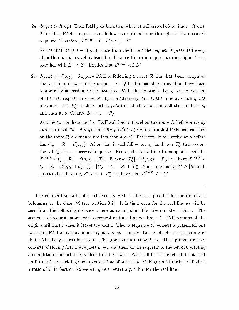
2a. d(o; x) > d(o; p). Then PAH goes back to o, where it will arrive before time t+d(o; x).After this, PAH computes and follows an optimal tour through all the unservedrequests. Therefore, ZPAH < t+ d(o; x) + jT �j.Notice that Z� � t + d(o; x), since from the time t the request is presented everyalgorithm has to travel at least the distance from the request to the origin. This,together with Z� � jT �j implies that ZPAH < 2 Z�.2b. d(o; x) � d(o; p). Suppose PAH is following a route R that has been computedthe last time it was at the origin. Let Q be the set of requests that have beentemporarily ignored since the last time PAH left the origin. Let q be the locationof the �rst request in Q served by the adversary, and tq the time at which q waspresented. Let P �Q be the shortest path that starts at q, visits all the points in Qand ends at o. Clearly, Z� � tq + jP �Qj.At time tq, the distance that PAH still has to travel on the route R before arrivingat o is at most jRj�d(o; q), since d(o; p(tq)) � d(o; q) implies that PAH has travelledon the route R a distance not less than d(o; q). Therefore, it will arrive at o beforetime tq + jRj � d(o; q). After that it will follow an optimal tour T �Q that coversthe set Q of yet unserved requests. Hence, the total time to completion will beZPAH � tq + jRj � d(o; q) + jT �Qj. Because jT �Qj � d(o; q) + jP �Qj, we have ZPAH �tq + jRj � d(o; q) + d(o; q) + jP �Qj = tq + jRj+ jP �Qj. Since, obviously, Z� � jRj and,as established before, Z� � tq + jP �Qj we have that ZPAH � 2 Z�. 2The competitive ratio of 2 achieved by PAH is the best possible for metric spacesbelonging to the class M (see Section 3.2). It is tight even for the real line as will beseen from the following instance where as usual point 0 is taken as the origin o. Thesequence of requests starts with a request at time 1 at position +1. PAH remains at theorigin until time 1 when it leaves towards 1. Then a sequence of requests is presented, oneeach time PAH arrives at point +�, at a point \slightly" to the left of ��, in such a waythat PAH always turns back to 0. This goes on until time 2 + �. The optimal strategyconsists of serving �rst the request in +1 and then all the requests to the left of 0 yieldinga completion time arbitrarily close to 2 + 2�, while PAH will be to the left of +� at leastuntil time 2+ �, yielding a completion time of at least 4. Making � arbitrarily small givesa ratio of 2. In Section 6.2 we will give a better algorithm for the real line.13

5 Polynomial time algorithms for OLTSPWe now turn the attention to polynomial time competitive algorithms for metric spacesbelonging to M. Even though competitiveness and computational complexity are notrelated concepts, for practical applications it is obviously relevant to make available poly-nomial time algorithms with a good competitive ratio.In the following we will present 3-competitive polynomial time algorithms for met-ric spaces belonging to M that use two well-known approximation algorithms for theEuclidean TSP as subroutine.5.1 A polynomial time algorithm for N-OLTSPOne known approximation algorithm for the Travelling Salesman Problem in which dis-tances satisfy the triangular inequality (�TSP) is the 2-approximate Minimum Span-ning Tree heuristic (e.g., see [14]). The MST heuristic provides a tour whose cost is atmost twice the length of a minimum spanning tree. This heuristic also provides a 2-approximation algorithm to the Hamiltonian Path Problem, since the size of a minimumspanning tree is a lower bound on the total length of an optimal Hamiltonian path.Let X be a set of points of the metric space M . We denote with MST (X) the sizeof the minimum spanning tree of the complete graph with set of vertices X, every edgebetween two points x, y in X is weighted with the distance d(x; y).Before presenting the algorithm, we give a preliminary lemma.Lemma 5.1 For every pair of points x and y in a set X, there exists a 2-approximatetour on X in which x and y are adjacent.Proof: Consider the minimum spanning tree over X. The MST heuristic consists ofdoubling all the edges of the tree, which yields an Eulerian graph, i.e., a connected graphin which all vertices have even degree. The total edge length of this graph is 2MST (X),which is at most twice the optimal tour length. We then use the fact that for any Euleriangraph and any edge in that graph, a standard short-cutting argument based on the triangleinequality will construct a TSP tour that contains that edge and has length no more thanthe sum of the graph's edge lengths. Now note that starting from the doubled tree, we willstill have an Eulerian graph if we replace a shortest path between x and y by a direct edgebetween x and y. This is because (a) all vertex degrees remain even (since the degrees ofx and y remain unchanged and those of the internal vertices of the path are reduced by14

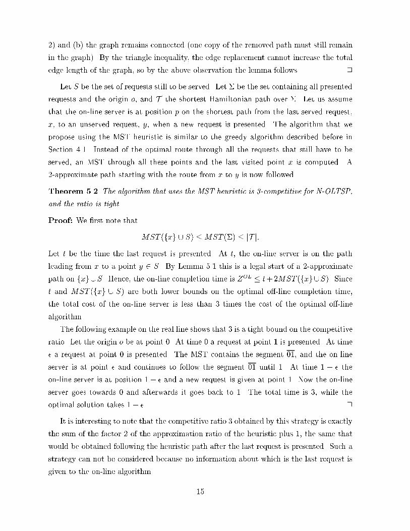
2) and (b) the graph remains connected (one copy of the removed path must still remainin the graph). By the triangle inequality, the edge replacement cannot increase the totaledge length of the graph, so by the above observation the lemma follows. 2Let S be the set of requests still to be served. Let � be the set containing all presentedrequests and the origin o, and T the shortest Hamiltonian path over �. Let us assumethat the on-line server is at position p on the shortest path from the last served request,x, to an unserved request, y, when a new request is presented. The algorithm that wepropose using the MST heuristic is similar to the greedy algorithm described before inSection 4.1. Instead of the optimal route through all the requests that still have to beserved, an MST through all these points and the last visited point x is computed. A2-approximate path starting with the route from x to y is now followed.Theorem 5.2 The algorithm that uses the MST heuristic is 3-competitive for N-OLTSP,and the ratio is tight.Proof: We �rst note that MST (fxg [ S) �MST (�) � jT j:Let t be the time the last request is presented. At t, the on-line server is on the pathleading from x to a point y 2 S. By Lemma 5.1 this is a legal start of a 2-approximatepath on fxg[S. Hence, the on-line completion time is ZOL � t+2MST (fxg[S). Sincet and MST (fxg [ S) are both lower bounds on the optimal o�-line completion time,the total cost of the on-line server is less than 3 times the cost of the optimal o�-linealgorithm.The following example on the real line shows that 3 is a tight bound on the competitiveratio. Let the origin o be at point 0. At time 0 a request at point 1 is presented. At time� a request at point 0 is presented. The MST contains the segment 01, and the on-lineserver is at point � and continues to follow the segment 01 until 1. At time 1 + � theon-line server is at position 1� � and a new request is given at point 1. Now the on-lineserver goes towards 0 and afterwards it goes back to 1. The total time is 3, while theoptimal solution takes 1 + �. 2It is interesting to note that the competitive ratio 3 obtained by this strategy is exactlythe sum of the factor 2 of the approximation ratio of the heuristic plus 1, the same thatwould be obtained following the heuristic path after the last request is presented. Such astrategy can not be considered because no information about which is the last request isgiven to the on-line algorithm. 15

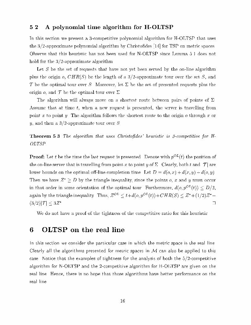
5.2 A polynomial time algorithm for H-OLTSPIn this section we present a 3-competitive polynomial algorithm for H-OLTSP that usesthe 3/2-approximate polynomial algorithm by Christo�des [14] for TSP on metric spaces.Observe that this heuristic has not been used for N-OLTSP since Lemma 5.1 does nothold for the 3/2-approximate algorithm.Let S be the set of requests that have not yet been served by the on-line algorithmplus the origin o, CHR(S) be the length of a 3/2-approximate tour over the set S, andT be the optimal tour over S. Moreover, let � be the set of presented requests plus theorigin o, and T be the optimal tour over �.The algorithm will always move on a shortest route between pairs of points of �.Assume that at time t, when a new request is presented, the server is travelling frompoint x to point y. The algorithm follows the shortest route to the origin o through x ory, and then a 3/2-approximate tour over S.Theorem 5.3 The algorithm that uses Christo�des' heuristic is 3-competitive for H-OLTSPProof: Let t be the time the last request is presented. Denote with pOL(t) the position ofthe on-line server that is travelling from point x to point y of �. Clearly, both t and jT j arelower bounds on the optimal o�-line completion time. Let D = d(o; x) + d(x; y)+ d(o; y).Then we have Z� � D by the triangle inequality, since the points o, x and y must occurin that order in some orientation of the optimal tour. Furthermore, d(o; pOL(t)) � D=2,again by the triangle inequality. Thus, ZOL � t+d(o; pOL(t))+CHR(S) � Z�+(1=2)Z�+(3=2)jT j � 3Z�. 2We do not have a proof of the tightness of the competitive ratio for this heuristic.6 OLTSP on the real lineIn this section we consider the particular case in which the metric space is the real line.Clearly all the algorithms presented for metric spaces in M can also be applied to thiscase. Notice that the examples of tightness for the analysis of both the 5/2-competitivealgorithm for N-OLTSP and the 2-competitive algorithm for H-OLTSP are given on thereal line. Hence, there is no hope that those algorithms have better performance on thereal line. 16

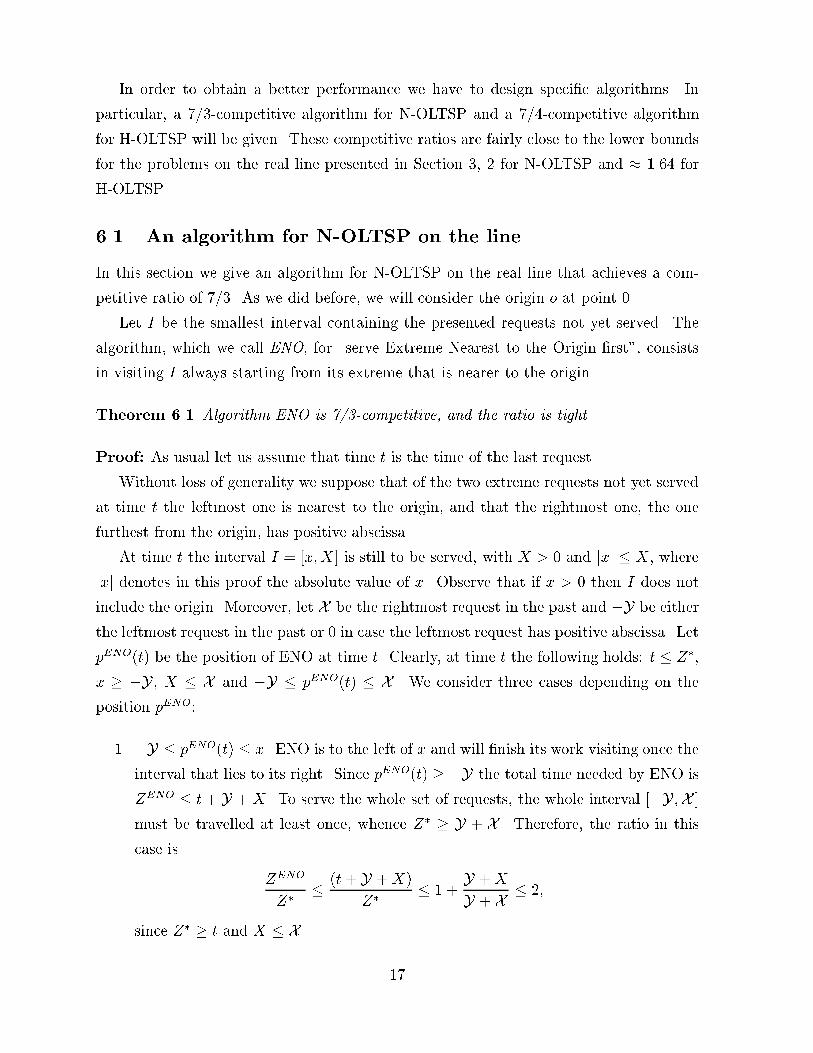
In order to obtain a better performance we have to design speci�c algorithms. Inparticular, a 7/3-competitive algorithm for N-OLTSP and a 7/4-competitive algorithmfor H-OLTSP will be given. These competitive ratios are fairly close to the lower boundsfor the problems on the real line presented in Section 3, 2 for N-OLTSP and � 1.64 forH-OLTSP.6.1 An algorithm for N-OLTSP on the lineIn this section we give an algorithm for N-OLTSP on the real line that achieves a com-petitive ratio of 7=3. As we did before, we will consider the origin o at point 0.Let I be the smallest interval containing the presented requests not yet served. Thealgorithm, which we call ENO, for \serve Extreme Nearest to the Origin �rst", consistsin visiting I always starting from its extreme that is nearer to the origin.Theorem 6.1 Algorithm ENO is 7/3-competitive, and the ratio is tight.Proof: As usual let us assume that time t is the time of the last request.Without loss of generality we suppose that of the two extreme requests not yet servedat time t the leftmost one is nearest to the origin, and that the rightmost one, the onefurthest from the origin, has positive abscissa.At time t the interval I = [x;X] is still to be served, with X > 0 and jxj � X, wherejxj denotes in this proof the absolute value of x. Observe that if x > 0 then I does notinclude the origin. Moreover, let X be the rightmost request in the past and �Y be eitherthe leftmost request in the past or 0 in case the leftmost request has positive abscissa. LetpENO(t) be the position of ENO at time t. Clearly, at time t the following holds: t � Z�,x � �Y, X � X and �Y � pENO(t) � X . We consider three cases depending on theposition pENO:1. �Y � pENO(t) � x. ENO is to the left of x and will �nish its work visiting once theinterval that lies to its right. Since pENO(t) � �Y the total time needed by ENO isZENO � t + Y +X. To serve the whole set of requests, the whole interval [�Y;X ]must be travelled at least once, whence Z� � Y + X . Therefore, the ratio in thiscase is ZENOZ� � (t+ Y +X)Z� � 1 + Y +XY + X � 2;since Z� � t and X � X . 17

2. x � pENO(t) � jxj, with x < 0 (this case coincides with the previous one if x > 0).In the worst case ENO is in position jxj and must visit �rst the leftmost extreme inposition x. The time needed by ENO is ZENO � t+ 3jxj+X. The optimal time isat least Z� � 2jxj+ X . From this and the assumption that jxj � X � X we haveZENOZ� � (t+ 3jxj+X)Z� � 1 + (3jxj+X)(2jxj+ X ) � 7=3:3. jxj < pENO(t) � X . We consider two di�erent cases:� In the optimal solution x is visited after X . Then we have Z� � 2X � x. Attime t ENO must cover at most twice the interval [x;X ], in case it is very closeto the rightmost extreme X . Then it will �nish by ZENO � t� 2x + 2X timeand the ratio is ZENOZ� � 1 + (�2x+ 2X )(�x + 2X ) � 7=3:� In the optimal solution X is visited after x. Suppose that the optimal o�-linealgorithm visits x at time d for the last time (with d � jxj, obviously). Then,at time d it still has to travel at least from x to X . Thus, Z� � d� x+X . Ifd � t we have that ZENOZ� � (d� 2x+ 2X )(d� x+ X ) � 2:Otherwise, if d < t, the following two claims hold:Claim 6.2 At every time t0, d � t0 � t, pENO(t0) � jxj.Proof: We prove this by contradiction. The time at which the request inposition x is presented is less than d since we assumed that at time d theoptimal o�-line algorithm has served x for the last time. Suppose ENO is inpENO(t0) � x at time t0. This implies that at time t the request in x has alreadybeen served since pENO(t) � x, which is a contradiction. This proves the claimfor x � 0. For x < 0, suppose x < pENO(t0) < jxj. Because x remains unservedat time t, ENO must have remained to the right of x until that time. Thus,since x is the leftmost unvisited request at time t, it also must have been so attime d. For ENO to end up to the right of jxj at time t, as we are assumingin this case, it would have to travel away from x. However, this could have18

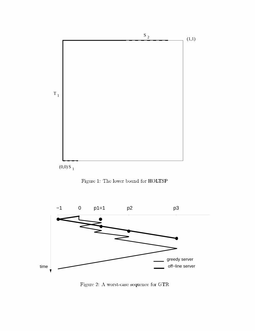
happened only so long as the rightmost unvisited request at the time was lessthan or equal to jxj, and so could not have caused ENO to be at the right ofjxj at time t, a contradiction. 2Claim 6.3 Starting at time d ENO moves to the left until time t.Proof: From the previous claim we know that between time d and time t ENOis always to the right of jxj. We notice that at any time during this periodthe extreme point of the interval of yet unserved requests that is nearest tothe origin must be inside [�jxj; jxj], implying that ENO always moves to theleft during this period. This can be readily seen from the fact that, given theprevious claim, during the whole period x always remains the leftmost pointnot yet served, and the on-line server is to the right of jxj at time t. 2Thus, at time d ENO starts from a position pENO(d) � jxj to travel to the leftand at time t it is still to the right of jxj. Therefore, ZENO � d + 2X � 2xyielding the ratio ZENOZ� � (d� 2x+ 2X )(d� x+ X ) � 2:We �nally prove that there is a sequence of requests for which ENO achieves a ratioof 7=3. This case is illustrated in Figure 3.At time 1 two requests in -1 and 1/2 are presented. At time 1 ENO leaves 0 towards1/2 and arrives at the origin at time 2 when a new request is presented in 1� �. Again,ENO goes to the right and arrives in 1� � at time 3 � �. At that time a new request isgiven in 1+� and ENO goes to the left since the extreme point in -1 is nearer to the originthan 1 + �. Altogether ENO takes time 7 � � to serve the requests, while the optimalo�-line solution needs 3 + �. The ratio tends to 7=3 as � tends to 0. 26.2 An algorithm for H-OLTSP on the lineIn this section we present an algorithm for H-OLTSP on the real line whose competitiveratio is 7/4. We call this algorithm PQR (for Possibly-Queue-Requests). As in PAH, the2-competitive algorithm for any metric space in M (see Section 4), PQR is based on theidea of postponing requests close to the origin.At any point in time let S be the set of requests unserved by PQR and let Q, thequeue, be the subset of S containing the requests that are temporarily ignored. PQR19

always follows the shortest tour from its current position through the set P = SnQ�nishing at the origin, followed by the shortest tour serving the requests in Q.PQR works in phases. The �rst phase starts with the �rst request, and each successivephase starts when a new request is presented that is not on the currently scheduled tourand whose absolute value is bigger than that of any other unserved request.At the beginning of a phase, PQR schedules the shortest route that, starting from itscurrent position pPQR(t), serves all the unserved requests and goes back to the origin. Wecall this route the greedy route. Requests may be presented during the phase. Some ofthem may call for computation of a new greedy route, while others are simply added toQ and cause a recomputation of the shortest tour through Q.We denote the current route remaining to be traversed as R, with R being the con-catenation of G, the part of the most recently computed greedy tour that remains to betraversed (and will visit all the cities in P) followed by H, the optimal tour for Q.During a phase, we refer to the long side as the half line from 0 on which the requestwhose presentation caused the start of the phase is located. The other side is then referredto as the short side.When a phase starts the set Q is empty. By the construction of our algorithm, Q willonly contain requests on the short side. Requests are removed from Q as soon as theyare served.PQR is described completely by its behavior when a new request is presented, say attime t.1. If the new request is on route R then proceed following R, add the request to P orQ, depending on whether it is �rst visited in G or H, and serve the request whenvisited; else2. If the new request is on the long side, then empty the set Q and rede�ne R as thenewly computed greedy route. If the new request is further from the origin thanany unserved request then also a new phase starts; else3. If the new request is on the short side and it is further from the origin than anyunserved request then a new phase starts, empty the set Q and rede�ne R as thenewly computed greedy route; else4. The request is on the short side but no new phase starts. Insert the request in Q,rede�ne H as the shortest tour that starts at the origin, visits all of Q, and returns.20

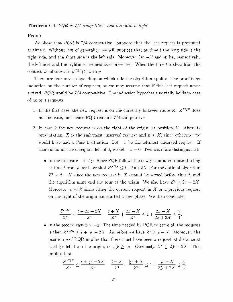
Theorem 6.4 PQR is 7/4-competitive, and the ratio is tight.Proof:We show that PQR is 7=4 competitive. Suppose that the last request is presentedat time t. Without loss of generality, we will suppose that at time t the long side is theright side, and the short side is the left side. Moreover, let �Y and X be, respectively,the leftmost and the rightmost request ever presented. When the time t is clear from thecontext we abbreviate pPQR(t) with p.There are four cases, depending on which rule the algorithm applies. The proof is byinduction on the number of requests, so we may assume that if this last request neverarrived, PQR would be 7=4 competitive. The induction hypothesis trivially holds in caseof no or 1 requests.1. In the �rst case, the new request is on the currently followed route R. ZPQR doesnot increase, and hence PQR remains 7/4 competitive.2. In case 2 the new request is on the right of the origin, at position X. After itspresentation, X is the rightmost unserved request and p � X, since otherwise wewould have had a Case 1 situation. Let �x be the leftmost unserved request. Ifthere is no unserved request left of 0, we set �x = 0. Two cases are distinguished:� In the �rst case �x < p. Since PQR follows the newly computed route startingat time t from p, we have that ZPQR � t+2x+2X. For the optimal algorithmZ� � t + X since the new request in X cannot be served before time t, andthe algorithm must end the tour at the origin. We also have Z� � 2x + 2X .Moreover, x � X since either the current request in X or a previous requeston the right of the origin has started a new phase. We then conclude:ZPQRZ� � t+ 2x+ 2XZ� = t +XZ� + 2x +XZ� � 1 + 2x+X2x + 2X � 74 :� In the second case p � �x. The time needed by PQR to serve all the requestsis then ZPQR � t + jpj + 2X. As before we have Z� � t +X. Moreover, theposition p of PQR implies that there must have been a request at distance atleast jpj left from the origin, i.e., Y � jpj. Obviously, Z� � 2Y + 2X. Thisimplies thatZPQRZ� � t + jpj+ 2XZ� = t+XZ� + jpj+XZ� � 1 + jpj+X2Y + 2X � 32 :21

3. In this case the new request is on the left of the origin at position �x. The newrequest is further from the origin than any other unserved request. Let X be therightmost unserved request. Clearly, X < x. If there is no unserved request to theright of 0, we set X = 0. At time t, p > �x, since otherwise we would have had aCase 1 situation. We distinguish two cases.� In the �rst case we have �x < p < X. Since PQR recomputes an optimalgreedy route at time t, we have ZPQR � t+2x+2X. For the optimal algorithmZ� � t+ x since the new request at position �x cannot be served before timet. Moreover, Z� � 2x+ 2X. We then obtain thatZPQRZ� � t+ 2x + 2XZ� = t + xZ� + x + 2XZ� � 1 + x + 2X2x+ 2X � 74 :� In the second case we have that p � X. The time needed by PQR to serve allthe requests and return to the origin is ZPQR � t+ jpj+2x, with jpj � X . Forthe optimal solution we have Z� � t+ x and Z� � 2x+2X . We conclude thatZPQRZ� � t+ jpj+ 2xZ� = t+ xZ� + x+ jpjZ� � 1 + x + X2x + 2X � 32 :4. In this case the request inserted into Q is further from the origin than any of theother unserved requests on the short side, but closer to the origin than the furthestunserved request on the long side. Let �x00 be the position of this request, �x0 andX 0 the leftmost and the rightmost unserved requests when the greedy tour was lastcomputed, and �x and X the leftmost and rightmost unserved requests when thecurrent phase started and so the current long side was declared to be such. Notethat we must have x00; x0; X 0 � X. We consider two subcases:� In the optimal solution X 0 is served before �x00. Let t0 be the time at which therequest in X 0 was presented, i.e., the time at which the current greedy routewas computed. For the optimal solution we get Z� � t0 +X 0 + 2x00.Another two subcases are distinguished, depending on pPQR(t0), i.e., the posi-tion of PQR at time t0, relative to the interval I = [�x0; X 0]:{ PQR was inside I at time t0. Notice that, at time t PQR is still working onthe greedy tour that was computed last since the request at t did not causea new phase. Therefore, ZPQR � t0+2x0+2X 0+2x00, while Z� � 2x0+2X.22

In this case the ratio isZPQRZ� � t0 + 2x0 + 2X 0 + 2x00Z� = t0 +X 0 + 2x00Z� + 2x0 +X 0Z�� 1 + 2x0 +X 02x0 + 2X � 74 ;since x0; X 0 � X.{ PQR was outside I at time t0. Observe that it could not be to the right ofX 0, otherwise a Case 1 situation would have occurred. Therefore, it wasnecessarily to the left of �x0. This implies that ZPQR � t0 + jpPQR(t0)j +2X 0 + 2x00. Obviously, jpPQR(t0)j � Y, and Z� � 2Y + 2X. Therefore,ZPQRZ� � t0 + jpPQR(t0)j+ 2X 0 + 2x00Z� = t0 +X 0 + 2x00Z� + jpPQR(t0)j+X 0Z�� 1 + jpPQR(t0)j+X 02Y + 2X � 32 :� In the optimal solution �x00 is served before X 0. Then, for the optimal solutionwe have Z� � t + x00 + 2X 0. Again, two subcases:{ PQR is to the right of �x0 at time t (it is certainly to the left of X 0). Weconsider two more subcases:� x0 < x00. Then ZPQR � t + 2x0 + 2X 0 + 2x00 while Z� � 2x00 + 2X. Inthis case the ratio isZPQRZ� � t+ 2x0 + 2X 0 + 2x00Z� = t+ 2X 0 + x00Z� + 2x0 + x00Z�� 1 + 2x0 + x002x00 + 2X � 74 :� x0 � x00. Since the request in �x00 is not visited on the current route,PQR has already visited x0 at time t and p > �x00. Then, ZPQR <t+ x00 + 2X 0 + 2x00 whereas Z� � 2x00 + 2X. The ratio isZPQRZ� � t+ x00 + 2X 0 + 2x00Z� = t + 2X 0 + x00Z� + 2x00Z�� 1 + 2x002x00 + 2X � 3=2;since x00 � X.{ PQR is to the left of �x0 at time t. p cannot be to the left of �x00 becausein that case �x00 would be on the current route, and therefore we have23

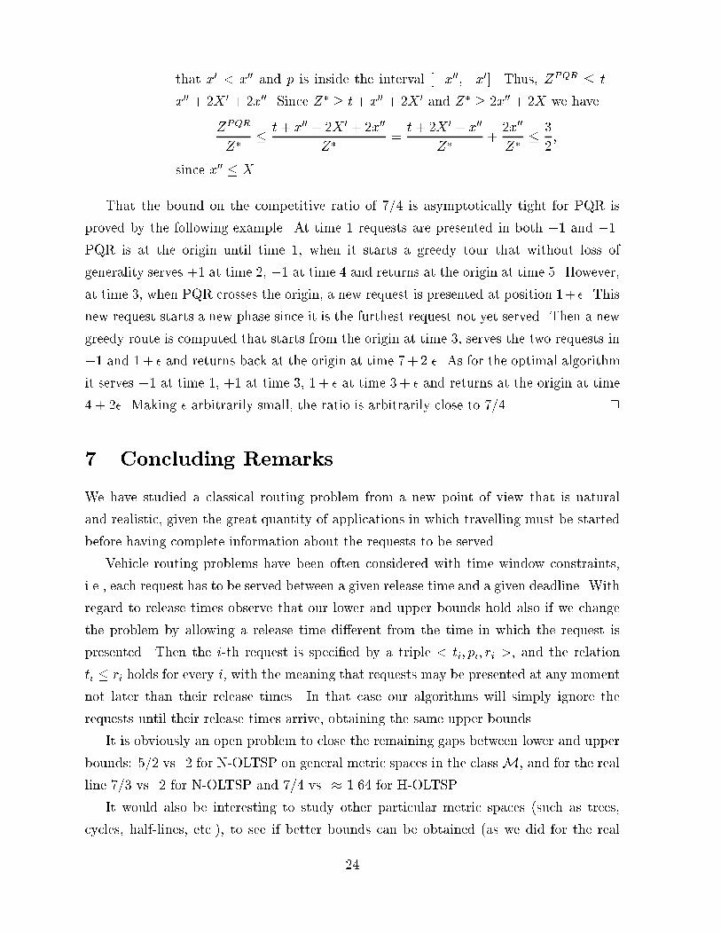
that x0 < x00 and p is inside the interval [�x00;�x0]. Thus, ZPQR � t +x00 + 2X 0 + 2x00. Since Z� � t+ x00 + 2X 0 and Z� � 2x00 + 2X we haveZPQRZ� � t+ x00 + 2X 0 + 2x00Z� = t+ 2X 0 + x00Z� + 2x00Z� � 32 ;since x00 � X.That the bound on the competitive ratio of 7=4 is asymptotically tight for PQR isproved by the following example. At time 1 requests are presented in both +1 and �1.PQR is at the origin until time 1, when it starts a greedy tour that without loss ofgenerality serves +1 at time 2, �1 at time 4 and returns at the origin at time 5. However,at time 3, when PQR crosses the origin, a new request is presented at position 1+ �. Thisnew request starts a new phase since it is the furthest request not yet served. Then a newgreedy route is computed that starts from the origin at time 3, serves the two requests in�1 and 1+ � and returns back at the origin at time 7+ 2 �. As for the optimal algorithmit serves �1 at time 1, +1 at time 3, 1 + � at time 3 + � and returns at the origin at time4 + 2�. Making � arbitrarily small, the ratio is arbitrarily close to 7=4. 27 Concluding RemarksWe have studied a classical routing problem from a new point of view that is naturaland realistic, given the great quantity of applications in which travelling must be startedbefore having complete information about the requests to be served.Vehicle routing problems have been often considered with time window constraints,i.e., each request has to be served between a given release time and a given deadline. Withregard to release times observe that our lower and upper bounds hold also if we changethe problem by allowing a release time di�erent from the time in which the request ispresented. Then the i-th request is speci�ed by a triple < ti; pi; ri >, and the relationti � ri holds for every i, with the meaning that requests may be presented at any momentnot later than their release times. In that case our algorithms will simply ignore therequests until their release times arrive, obtaining the same upper bounds.It is obviously an open problem to close the remaining gaps between lower and upperbounds: 5/2 vs. 2 for N-OLTSP on general metric spaces in the classM, and for the realline 7/3 vs. 2 for N-OLTSP and 7/4 vs. � 1.64 for H-OLTSP.It would also be interesting to study other particular metric spaces (such as trees,cycles, half-lines, etc.), to see if better bounds can be obtained (as we did for the real24

line).An interesting extension of OLTSP is to crew scheduling in which more than oneserver is used to serve the requests. In this case a 2.5-competitive algorithm can be easilyobtained for the Homing version of this on-line problem by the following strategy workingin phases: Each time a new request is presented, all the servers return to the origin andplan an optimal tour for covering all the unserved requests, (and eventually end to theorigin). However, improvements are certainly possible.Other possible extensions of the problems considered in this paper may take intoaccount di�erent objective functions. For instance consider the sum (or the average) overall the requests of the individual service times, de�ned as the time at which the requestis served, or of the individual service delays, de�ned as the interval between the time atwhich the request is presented and the time at which the request is served.A second class of problems that may be considered is provided by the dial-a-ridescenario, in which each request consists of moving an item located at a certain positionin the metric space to a second position in the metric space. Examples of such problems(with multiple servers) are a system of taxis in a city or a system of elevators. Noticethat in those cases one might wish to impose an extra constraint covering the capacity ofthe server.AcknowledgmentsWe are grateful to David Johnson for his extensive comments on an earlier version of thispaper.References[1] H. Alborzi, E. Torng, P. Uthaisombut and S. Wagner, The k-client problem, Proc.Eighth Annual ACM-SIAM Symposium on Discrete Algorithms, (1997), pp. 73-82.[2] M. Atallah and S. Kosaraju, E�cient solutions for some transportation problemswith application to minimizing robot arm travel, SIAM J. on Computing, 17 (1988),pp. 849-869.[3] A. Borodin and R. El-Yaniv,On-line computation and competitive analysis, Cam-bridge University Press, Cambridge UK, 1998.25

[4] S. Ben-David, A. Borodin, R.M. Karp, G. Tardos and A. Widgerson, On the powerof randomization in on-line algorithms. Proc of the 22nd Annual ACM Symposiumon Theory of Computing, pp. 379-386, 1990.[5] R. El-Yaniv, A. Fiat, R.M. Karp and G. Turpin, Competitive analysis of �nancialgames, Proc. 33rd Annual Symposium on Foundations of Computer Science (1992),pp. 327-333.[6] G. Frederickson, A note on the complexity of a simple transportation problem,SIAM J. on Computing, 22-1 (1993), pp. 57-61.[7] G. Frederickson and D. Guan, Preemptive ensemble motion planning on a tree,SIAM J. on Computing, 21-6 (1992), pp. 1130-1152.[8] G. Frederickson, M. Hecht and C. Kim, Approximation algorithms for some routingproblems, SIAM J. on Computing, 7-2 (1978), pp. 178-193.[9] M. Garey, and D. Johnson, Computers and intractability: a guide to the theory ofNP-completeness, Freeman, San Francisco (1979).[10] R.L. Graham, \Bounds for certain multiprocessing anomalies", Bell System Tech-nical Journal 45 (1966), pp. 1563-1581.[11] D.S. Johnson. Near optimal bin-packing algorithms. Doctoral thesis, MIT, 1973.[12] Y. Karuno, H. Nagamochi and T. Ibaraki, Vehicle scheduling on a tree with releasetimes and handling times, Proc. 4th. International Symposium on Algorithms andComputation ISAAC'93, LNCS 762 (1993), Springer-Verlag, pp. 486-495.[13] B. Kalyanasundaram and K.R. Pruhs, Constructing competitive tours from localinformation, Proc. 20th International Colloquium on Automata, Languages and Pro-gramming, LNCS 700 (1993), Springer-Verlag.[14] E.L. Lawler, J.K. Lenstra, A.H.G. Rinnooy Kan and D.B. Shmoys (eds.), Thetravelling salesman problem: a guided tour of combinatorial optimization, Wiley,Chichester (1985).[15] M. Manasse, L.A. McGeoch and D. Sleator, Competitive algorithms for server prob-lems, Journal of Algorithms 11 (1990), pp. 208-230.26

[16] H. Psaraftis, M. Solomon, T. Magnanti and T. Kim, Routing and scheduling on ashoreline with release times, Management Science 36-2 (1990), pp. 212-223.[17] D.B. Shmoys, J. Wein, D.P. Williamson, \Scheduling parallel machines on-line",Proc. of the 32nd Annual Symposium on Foundations of Computer Science, 1991.[18] D. Sleator, R. Tarjan, Amortized e�ciency of list update and paging algorithms,Comm. ACM 28 (1985), pp. 202-208.[19] D. Sleator, R. Tarjan, Self-adjusting binary search trees, Journal of the ACM, 32(1985), pp. 652-686.[20] M. Solomon, \Algorithms for the vehicle routing and scheduling problem with timewindow constraints", Operations Research, 35-2 (1987), pp. 254-265.[21] M. Solomon and J. Desrosiers, \Time window constrained routing and schedulingproblems: a survey", Transportation Science, 22 (1988), pp. 1-13.

27

(0,0)

(1,1)

T

S

S

1

2

1 Figure 1: The lower bound for HOLTSP−1 0 p1=1 p2 p3

time

greedy server

off−line serverFigure 2: A worst-case sequence for GTR

greedy server

off−line server

time

10 0.5−1

Figure 3: A worst-case sequence for the ENO algorithm

29