Algorithms for time-optimal control of CNC machines along

Algorithms for time-optimal controlof CNC machines along curved tool paths

dramatis personæ(in alphabetical order):

Casey L. Boyadjieff, MS student

Rida T. Farouki, head honcho

Tait S. Smith, post-doctorus emeritus

Sebastian D. Timar, PhD aspirant

— scene of the crime —

Mechanical & Aeronautical Engineering, UC Davis

the time optimal control problem

It has been an intuitive assumption for some time that if acontrol system is being operated from a limited source ofpower, and if one wishes to have the system change fromone state to another in minimum time, then this can be doneby at all times utilizing properly all of the power available.This hypothesis is called “the bang-bang principle.”

Bushaw accepted this hypothesis, and in 1952 showed forsome simple systems with one degree of freedom that,of allbang-bang systems, there is one that is optimal. In 1953, Imade the observation that the best of all bang-bang systems,if it exists, is then the best of all systems operating from thesame power source.

J. P. La Salle (1960)

prior work (robotics literature)

J. E. Bobrow, S. Dubowsky, and J. S. Gibson (1985), Time-optimal control of robotic manipulatorsalong specified paths, International Journal of Robotics Research 4 (3), 3–17

F. Pfeiffer and R. Johanni (1987), A concept for manipulator trajectory planning,IEEE Journal of Robotics and Automation RA–3 (2), 115–123

Z. Shiller (1994), On singular time–optimal control along specified paths,IEEE Transactions on Robotics and Automation 10, 561–566

Z. Shiller and H. H. Lu (1990), Robust computation of path constrained time optimal motions,Proceedings, IEEE International Conference on Robotics and Automation, 144–149

Z. Shiller and H. H. Lu (1992), Computation of path constrained time optimal motions with dynamicsingularities, Journal of Dynamic Systems, Measurement, and Control 114 (March), 34–40

K. G. Shin and N. D. McKay (1985), Minimum-time control of robotic manipulators with geometricpath contraints, IEEE Transactions on Automatic Control AC-30 (6), 531–541

J. J. E. Slotine and H. S. Yang (1989), Improving the efficiency of time–optimal path–followingalgorithms, IEEE Transaction on Robotics and Automation 5 (1), 118–124

H. S. Yang and J. J. E. Slotine (1994), Fast algorithms for near–minimum–time controlof robot manipulators, International Journal of Robotics Research 13, 521–532

attractive features of Cartesian problem

• closed-form integration of v = amin/max(s, v) ODEs

• ⇒ (optimal feedrate)2 = piecewise-rational function

• switching points = roots of univariate polynomials

• analytic reduction of “interpolation integral”⇒ accurate & efficient real-time interpolator

• amenable to all types of (piecewise) polynomialparametric curves (Bezier, B-spline, etc.)

“conventional” vs. “high-speed” machining

• machining times are major determinant of product cost

• usual: feedrate ≤ 100 in/min, spindle speed ≤ 6, 000 rpm

• HSM: feedrate ≤ 1, 200 in/min, spindle speed ≤ 50, 000 rpm

• in HSM inertial effects may dominate cutting forces, friction, etc.(especially for intricate curved tool paths)

• most CNC machines significantly under-perform in practice– control software, not hardware, is the limiting factor

• determine feedrate for minimal-time traversal of curved path, undergiven axis acceleration bounds (assuming inertial forces dominant)

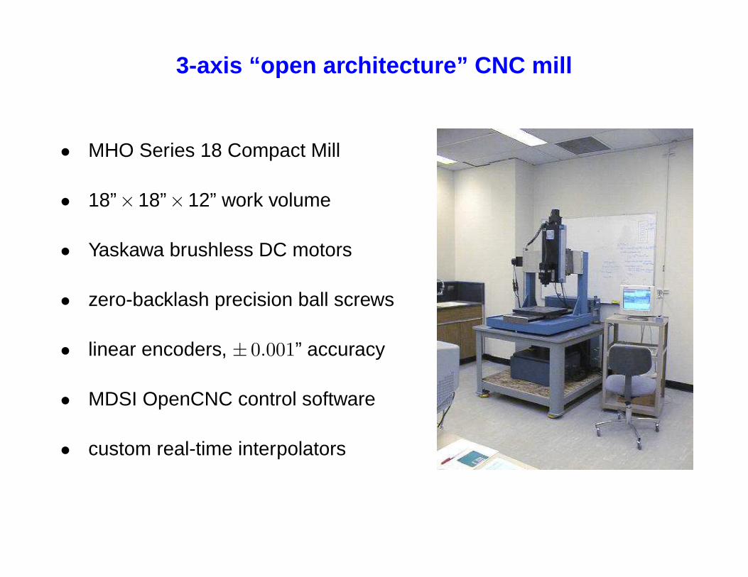
3-axis “open architecture” CNC mill

• MHO Series 18 Compact Mill

• 18”×18”×12” work volume

• Yaskawa brushless DC motors

• zero-backlash precision ball screws

• linear encoders, ± 0.001” accuracy

• MDSI OpenCNC control software

• custom real-time interpolators

��

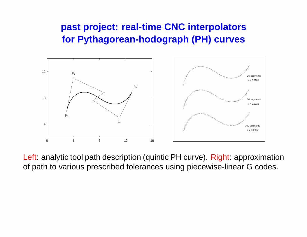
past project: real-time CNC interpolatorsfor Pythagorean-hodograph (PH) curves

0 4 8 12 16

4

8

12

p0

p1

p4

p5

25 segments

ε = 0.0105

50 segments

ε = 0.0025

100 segments

ε = 0.0006

Left: analytic tool path description (quintic PH curve). Right: approximationof path to various prescribed tolerances using piecewise-linear G codes.

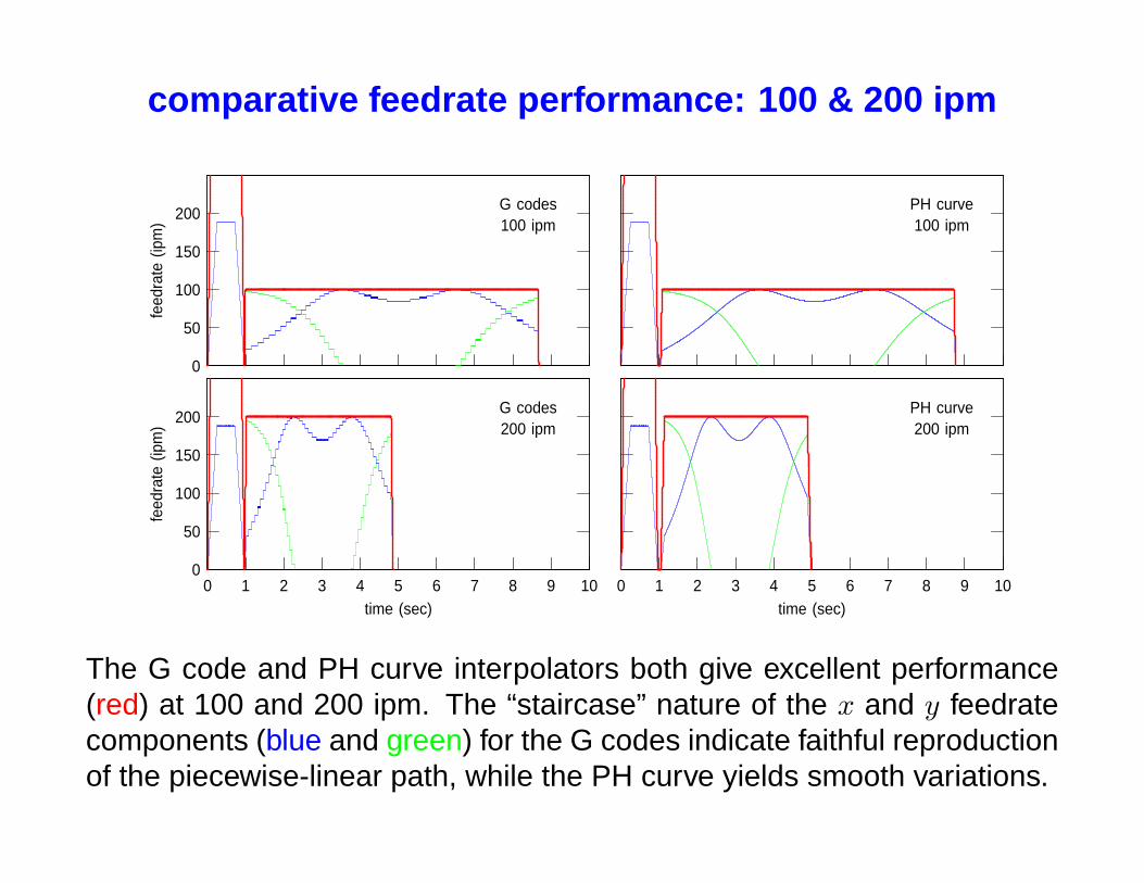
comparative feedrate performance: 100 & 200 ipm

0 1 2 3 4 5 6 7 8 9 100

50

100

150

200

time (sec)

feed

rate

(ip

m)

G codes200 ipm

0

50

100

150

200

feed

rate

(ip

m)

G codes100 ipm

0 1 2 3 4 5 6 7 8 9 10time (sec)

PH curve200 ipm

PH curve100 ipm

The G code and PH curve interpolators both give excellent performance(red) at 100 and 200 ipm. The “staircase” nature of the x and y feedratecomponents (blue and green) for the G codes indicate faithful reproductionof the piecewise-linear path, while the PH curve yields smooth variations.

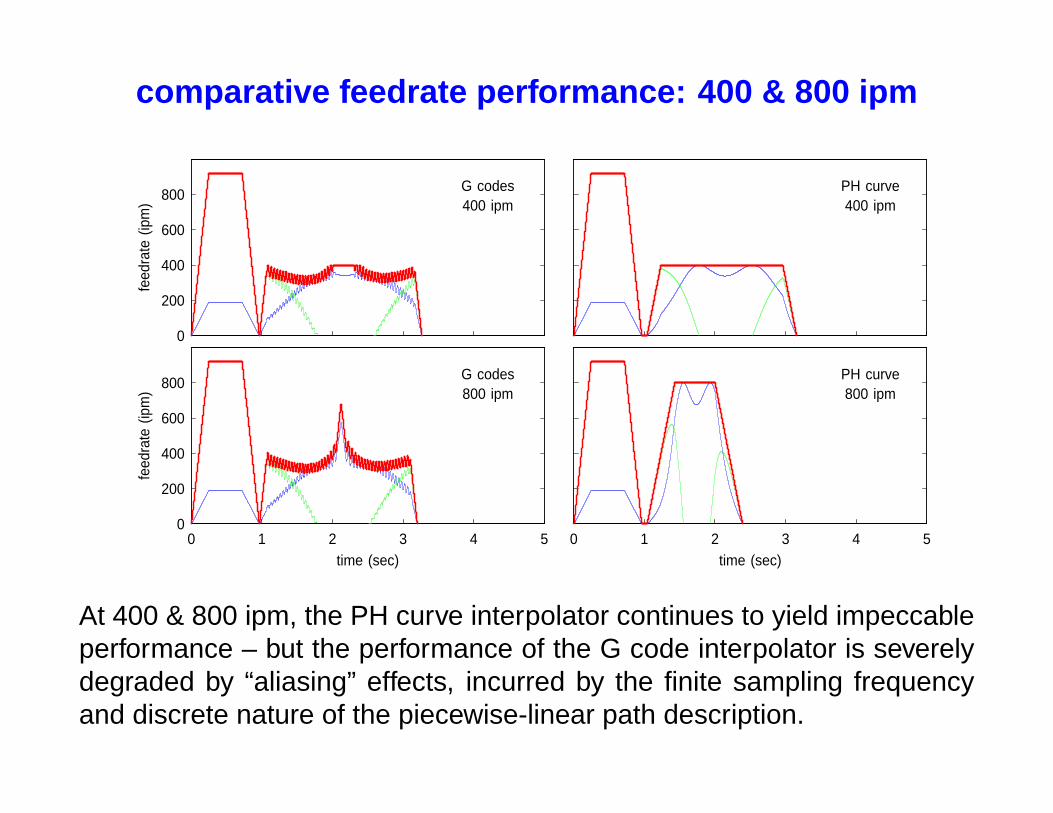
comparative feedrate performance: 400 & 800 ipm

0 1 2 3 4 50

200

400

600

800

time (sec)

feed

rate

(ip

m)

G codes800 ipm

0

200

400

600

800

feed

rate

(ip

m)

G codes400 ipm

0 1 2 3 4 5time (sec)

PH curve800 ipm

PH curve400 ipm

At 400 & 800 ipm, the PH curve interpolator continues to yield impeccableperformance – but the performance of the G code interpolator is severelydegraded by “aliasing” effects, incurred by the finite sampling frequencyand discrete nature of the piecewise-linear path description.

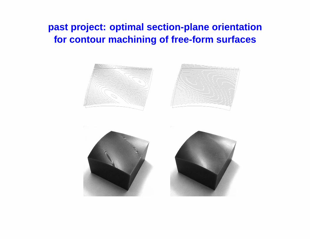
past project: optimal section-plane orientationfor contour machining of free-form surfaces

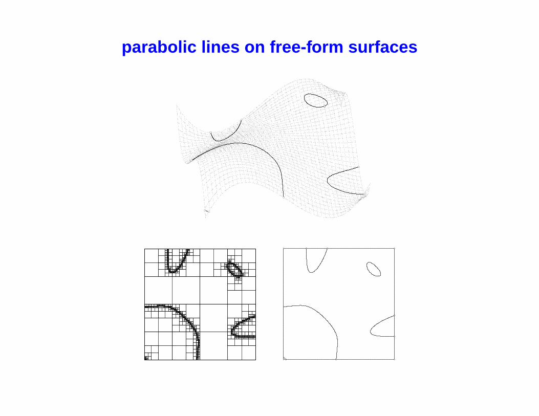
parabolic lines on free-form surfaces

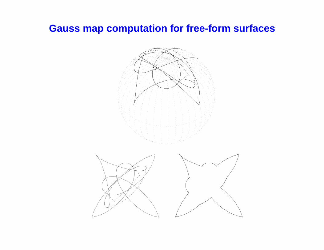
Gauss map computation for free-form surfaces

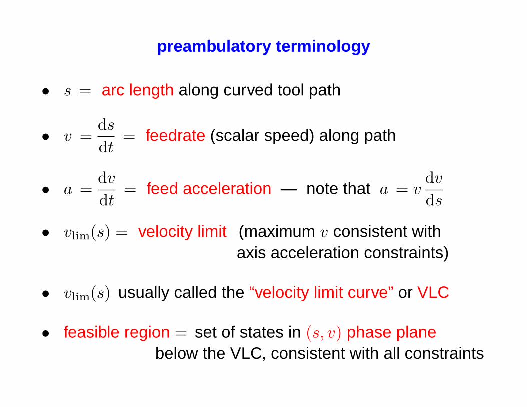
preambulatory terminology

• s = arc length along curved tool path

• v =ds

dt= feedrate (scalar speed) along path

• a =dv

dt= feed acceleration — note that a = v

dv

ds

• vlim(s) = velocity limit (maximum v consistent withaxis acceleration constraints)

• vlim(s) usually called the “velocity limit curve” or VLC

• feasible region = set of states in (s, v) phase planebelow the VLC, consistent with all constraints

time-optimal motion with acceleration constraints

κ > 0 κ = 0 κ < 0

aκ v2

a

a

κ v2

acceleration vector r = a t + κv2 n

t = tangent, n = normal, κ = curvature, v = feedrate, a = feed acceleration

minv

T =∫

ds

vsuch that

−Ax ≤ a tx + κv2nx ≤ +Ax

−Ay ≤ a ty + κv2ny ≤ +Ay

−Az ≤ a tz + κv2nz ≤ +Az

for simplicity, take Ax = Ay = Az (= A, say) henceforth

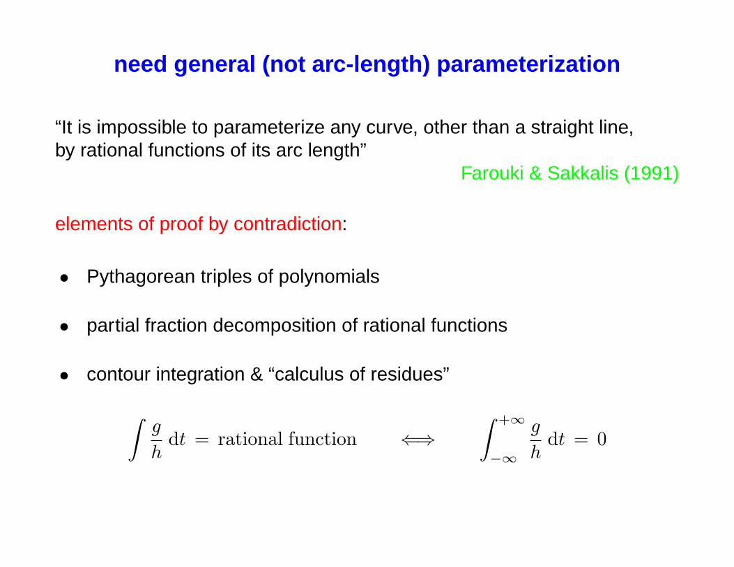
need general (not arc-length) parameterization

“It is impossible to parameterize any curve, other than a straight line,by rational functions of its arc length”

Farouki & Sakkalis (1991)

elements of proof by contradiction:

• Pythagorean triples of polynomials

• partial fraction decomposition of rational functions

• contour integration & “calculus of residues”

∫g

hdt = rational function ⇐⇒

∫ +∞

−∞

g

hdt = 0

degree–n Bezier curve

r(ξ) = (x(ξ), y(ξ), z(ξ)) =n∑

k=0

pk

(n

k

)(1− ξ)n−kξk , ξ ∈ [ 0, 1 ]

denote ξ-derivatives by primes & define parametric speed

σ(ξ) = |r′(ξ)| =ds

dξ

with q = v2 (and hence q′ = 2σa) acceleration constraints become

−A ≤ q′

2σ2x′ +

q

σ3(σx′′ − σ′x′) ≤ +A

−A ≤ q′

2σ2y′ +

q

σ3(σy′′ − σ′y′) ≤ +A

−A ≤ q′

2σ2z′ +

q

σ3(σz′′ − σ′z′) ≤ +A

for ξ ∈ [ 0, 1 ]

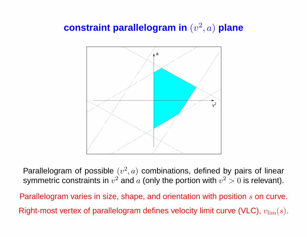
constraint parallelogram in (v2, a) plane

a

v2

Parallelogram of possible (v2, a) combinations, defined by pairs of linearsymmetric constraints in v2 and a (only the portion with v2 > 0 is relevant).

Parallelogram varies in size, shape, and orientation with position s on curve.

Right-most vertex of parallelogram defines velocity limit curve (VLC), vlim(s).

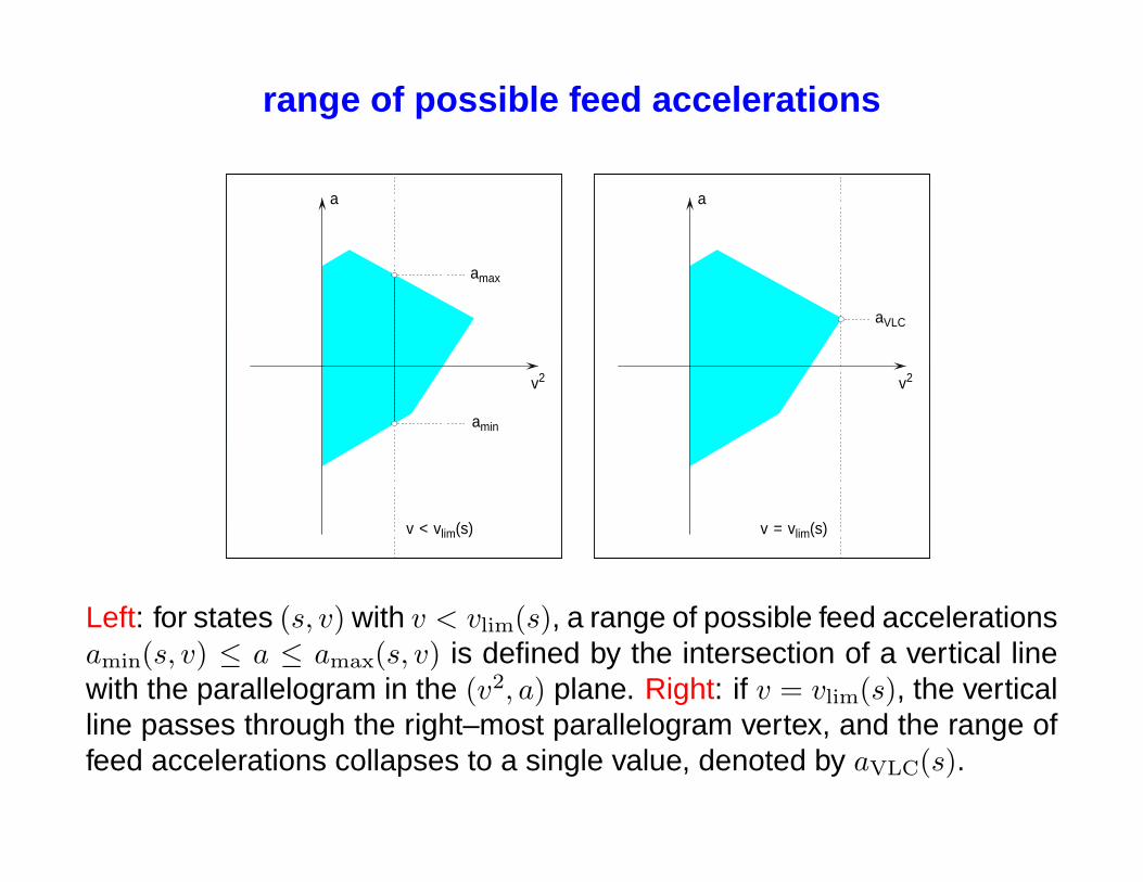
range of possible feed accelerations

v < vlim(s)

amin

amax

a

v2

v = vlim(s)

aVLC

a

v2

Left: for states (s, v) with v < vlim(s), a range of possible feed accelerationsamin(s, v) ≤ a ≤ amax(s, v) is defined by the intersection of a vertical linewith the parallelogram in the (v2, a) plane. Right: if v = vlim(s), the verticalline passes through the right–most parallelogram vertex, and the range offeed accelerations collapses to a single value, denoted by aVLC(s).

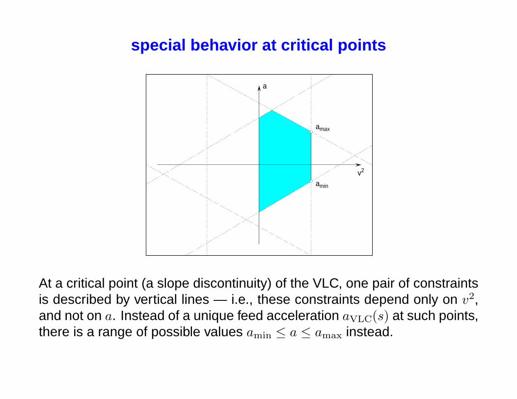
special behavior at critical points

amin

amax

a

v2

At a critical point (a slope discontinuity) of the VLC, one pair of constraintsis described by vertical lines — i.e., these constraints depend only on v2,and not on a. Instead of a unique feed acceleration aVLC(s) at such points,there is a range of possible values amin ≤ a ≤ amax instead.

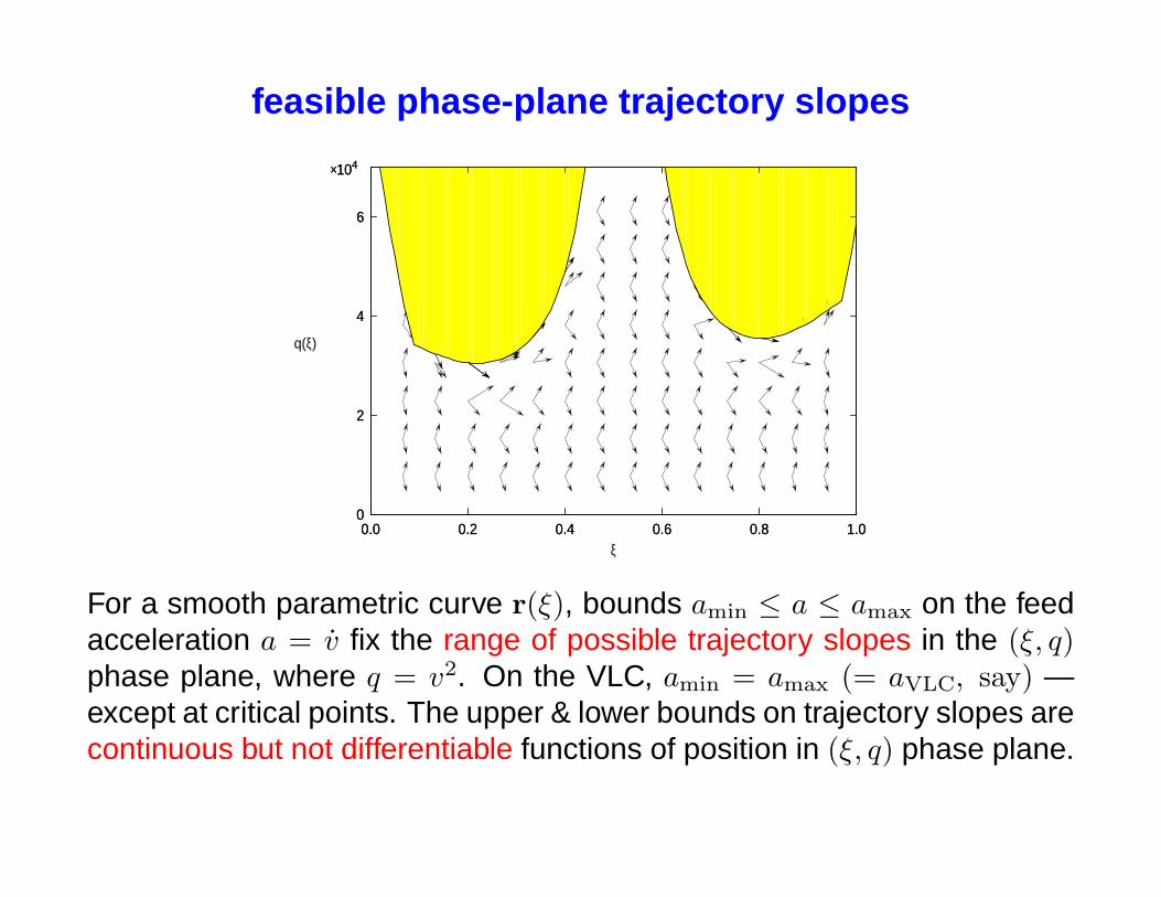
feasible phase-plane trajectory slopes

0.0 0.2 0.4 0.6 0.8 1.00

2

4

6

×104

ξ

q(ξ)

0.0 0.2 0.4 0.6 0.8 1.00

2

4

6

×104

For a smooth parametric curve r(ξ), bounds amin ≤ a ≤ amax on the feedacceleration a = v fix the range of possible trajectory slopes in the (ξ, q)phase plane, where q = v2. On the VLC, amin = amax (= aVLC, say) —except at critical points. The upper & lower bounds on trajectory slopes arecontinuous but not differentiable functions of position in (ξ, q) phase plane.

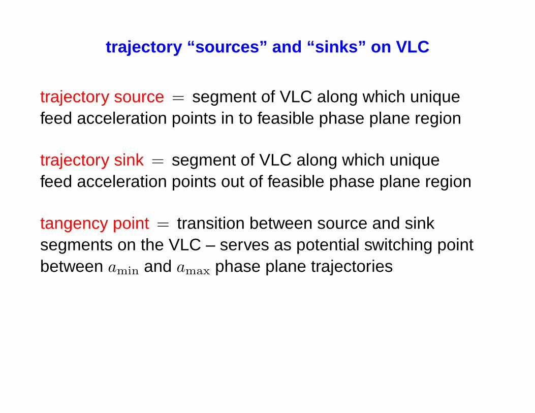
trajectory “sources” and “sinks” on VLC

trajectory source = segment of VLC along which uniquefeed acceleration points in to feasible phase plane region

trajectory sink = segment of VLC along which uniquefeed acceleration points out of feasible phase plane region

tangency point = transition between source and sinksegments on the VLC – serves as potential switching pointbetween amin and amax phase plane trajectories

we interrupt this seminar for a

— BREAKING NEWS FLASH !! —

Hu is the new leader of China ?(transcript of a White House conversation between George W. Bush and Condoleeza Rice

upon the nomination of Hu Jintao as the new Chief of the Communist Party of China)

• George : Condi! Nice to see you. What’s happening?

• Condi : Sir, I have here the report about the new leader of China.

• George : Great. Lay it on me.

• Condi : Hu is the new leader of China.

• George : That’s what I want to know.

• Condi : That’s what I’m telling you.

• George : That’s what I’m asking you. Who is the new leader of China?

• Condi : Yes.

• George : I mean the fellow’s name.

• Condi : Hu.

• George : The guy in China.

• Condi : Hu.

• George : The new leader of China.

• Condi : Hu.

• George : The Chinaman!

• Condi : Hu is leading China.

• George : Now whaddya’ asking me for?

• Condi : I’m telling you Hu is leading China.

• George : Well, I’m asking you. Who is leading China?

• Condi : That’s the man’s name.

• George : That’s who’s name?

• Condi : Yes.

• George : Will you or will you not tell me the name of the new leader of China?

• Condi : Yes, sir.

• George : Yassir? Yassir Arafat is in China? I thought he was in the Middle East.

• Condi : That’s correct.

• George : Then who is in China?


• George : Yassir is in China?

• Condi : No, sir.

• George : Then who is?


• George : Yassir?

• Condi : No, sir.

• George : Look, Condi. I need to know the name of the new leader of China.Get me the Secretary General of the UN on the phone.

• Condi : Kofi?

• George : No, thanks.

• Condi : You want Kofi?

• George : No.

• Condi : You don’t want Kofi.

• George : No. But now that you mention it, I could use a glass of milk. And then get me the UN.


• George : Not Yassir! The guy at the UN.

• Condi : Kofi?

• George : Milk! Will you please make the call?

• Condi : And call who?

• George : Who is the guy at the UN?

• Condi : Hu is the guy in China.

• George : Will you stay out of China?!


• George : And stay out of the Middle East! Just get me the guy at the UN.

• Condi : Kofi.

• George : All right! With cream and two sugars. Now get on the phone. (Condi picks up the phone.)

• Condi : Rice, here.

• George : Rice? Good idea. And a couple of egg rolls, too. Maybe we should send some to the guyin China. And the Middle East. Can you get Chinese food in the Middle East?

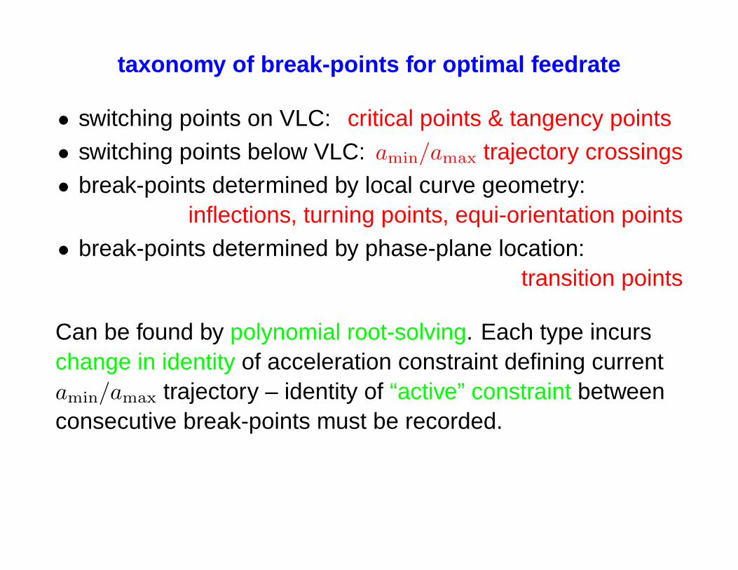
taxonomy of break-points for optimal feedrate

• switching points on VLC: critical points & tangency points

• switching points below VLC: amin/amax trajectory crossings

• break-points determined by local curve geometry:inflections, turning points, equi-orientation points

• break-points determined by phase-plane location:transition points

Can be found by polynomial root-solving. Each type incurschange in identity of acceleration constraint defining currentamin/amax trajectory – identity of “active” constraint betweenconsecutive break-points must be recorded.

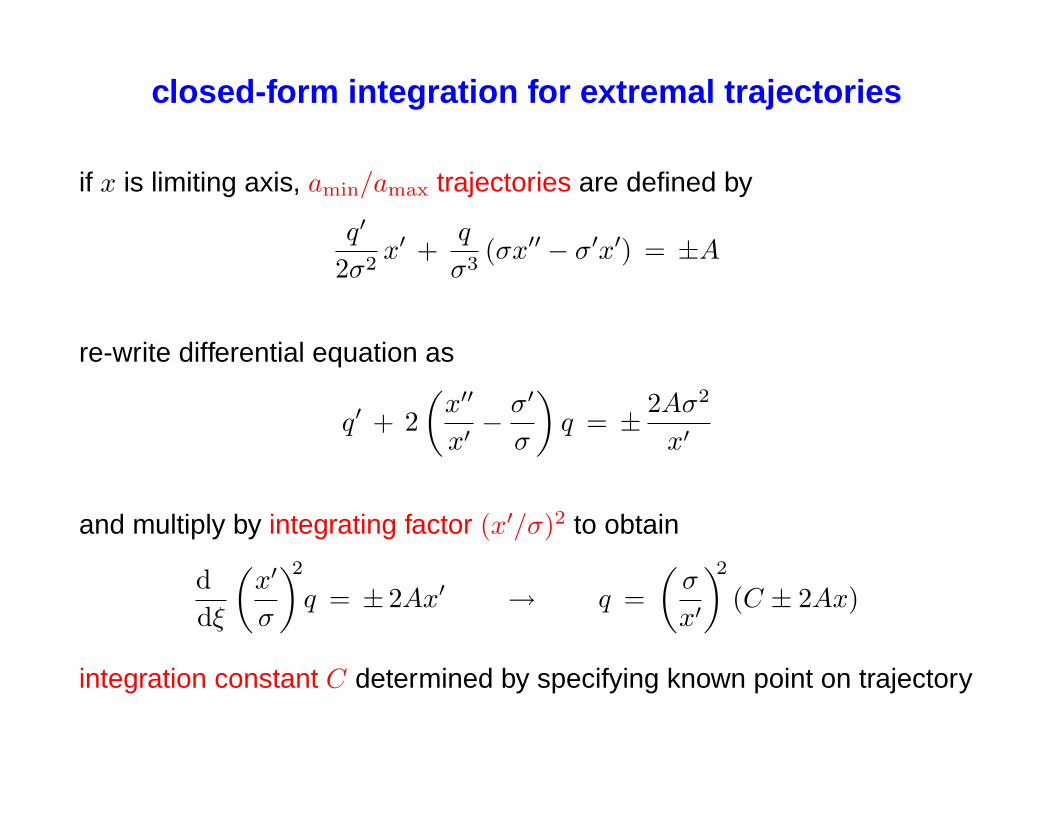
closed-form integration for extremal trajectories

if x is limiting axis, amin/amax trajectories are defined by

q′

2σ2x′ +

q

σ3(σx′′ − σ′x′) = ±A

re-write differential equation as

q′ + 2(

x′′

x′− σ′

σ

)q = ± 2Aσ2

x′

and multiply by integrating factor (x′/σ)2 to obtain

ddξ

(x′

σ

)2

q = ± 2Ax′ → q =(

σ

x′

)2

(C ± 2Ax)

integration constant C determined by specifying known point on trajectory

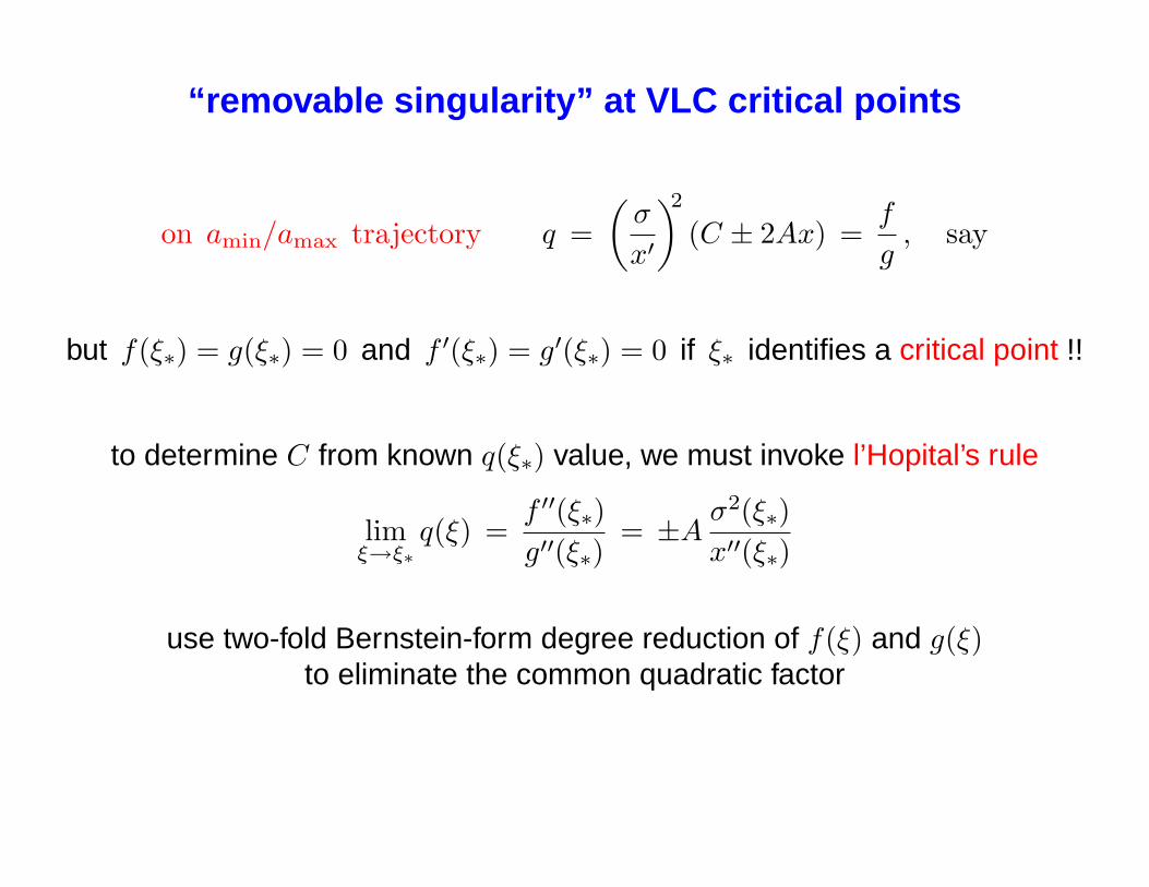
“removable singularity” at VLC critical points

on amin/amax trajectory q =(

σ

x′

)2

(C ± 2Ax) =f

g, say

but f(ξ∗) = g(ξ∗) = 0 and f ′(ξ∗) = g′(ξ∗) = 0 if ξ∗ identifies a critical point !!

to determine C from known q(ξ∗) value, we must invoke l’Hopital’s rule

limξ→ξ∗

q(ξ) =f ′′(ξ∗)g′′(ξ∗)

= ±Aσ2(ξ∗)x′′(ξ∗)

use two-fold Bernstein-form degree reduction of f(ξ) and g(ξ)to eliminate the common quadratic factor

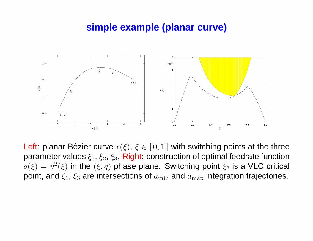
simple example (planar curve)

0 1 2 3 4 5

0

1

2

3

x [in]

y [in

]

ξ = 0

ξ1

ξ2ξ3

ξ = 1

0.0 0.2 0.4 0.6 0.8 1.00

1

2

3

4

5

×104

0.0 0.2 0.4 0.6 0.8 1.00

1

2

3

4

5

×104

ξ

q(ξ)

Left: planar Bezier curve r(ξ), ξ ∈ [ 0, 1 ] with switching points at the threeparameter values ξ1, ξ2, ξ3. Right: construction of optimal feedrate functionq(ξ) = v2(ξ) in the (ξ, q) phase plane. Switching point ξ2 is a VLC criticalpoint, and ξ1, ξ3 are intersections of amin and amax integration trajectories.

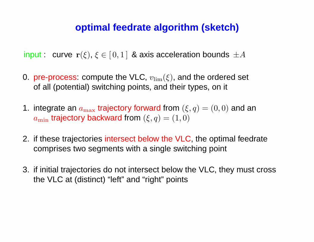
optimal feedrate algorithm (sketch)

input : curve r(ξ), ξ ∈ [ 0, 1 ] & axis acceleration bounds ±A

0. pre-process: compute the VLC, vlim(ξ), and the ordered setof all (potential) switching points, and their types, on it

1. integrate an amax trajectory forward from (ξ, q) = (0, 0) and anamin trajectory backward from (ξ, q) = (1, 0)

2. if these trajectories intersect below the VLC, the optimal feedratecomprises two segments with a single switching point

3. if initial trajectories do not intersect below the VLC, they must crossthe VLC at (distinct) “left” and “right” points

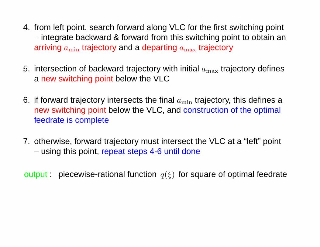
4. from left point, search forward along VLC for the first switching point– integrate backward & forward from this switching point to obtain anarriving amin trajectory and a departing amax trajectory

5. intersection of backward trajectory with initial amax trajectory definesa new switching point below the VLC

6. if forward trajectory intersects the final amin trajectory, this defines anew switching point below the VLC, and construction of the optimalfeedrate is complete

7. otherwise, forward trajectory must intersect the VLC at a “left” point– using this point, repeat steps 4-6 until done

output : piecewise-rational function q(ξ) for square of optimal feedrate

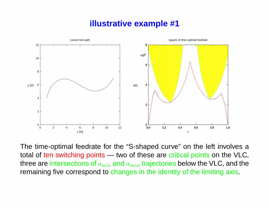
illustrative example #1

0.0 0.2 0.4 0.6 0.8 1.00

2

4

6

8

×104

0.0 0.2 0.4 0.6 0.8 1.00

2

4

6

8

×104

ξ

q(ξ)

square of time–optimal feedrate

0 2 4 6 8 10 120

2

4

6

8

10

12

x [in]

y [in]

curved tool path

The time-optimal feedrate for the “S-shaped curve” on the left involves atotal of ten switching points — two of these are critical points on the VLC,three are intersections of amin and amax trajectories below the VLC, and theremaining five correspond to changes in the identity of the limiting axis.


0.0 0.2 0.4 0.6 0.8 1.00

2

4

6

8

×104


ξ

q(ξ)

0.0 0.2 0.4 0.6 0.8 1.00

2

4

6

8

×104

curved tool path

0 1 2 3 4 5 6 70

1

2

3

4

5

6

7

x [in]

y [in]

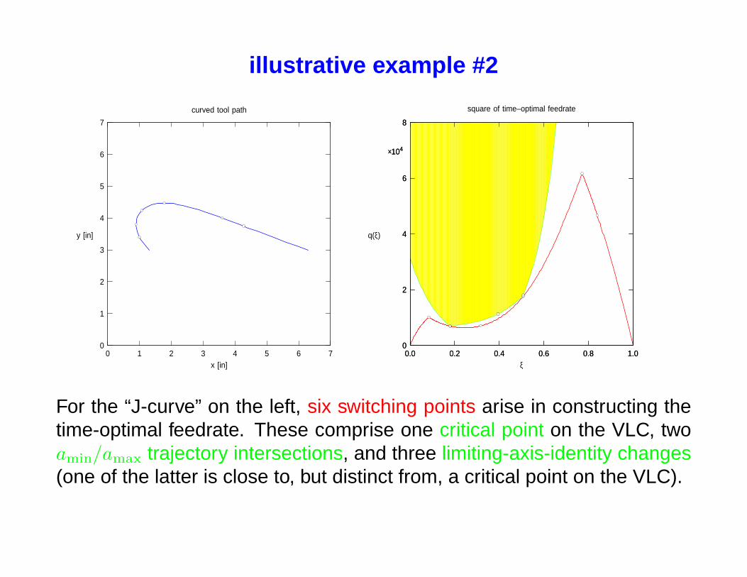
For the “J-curve” on the left, six switching points arise in constructing thetime-optimal feedrate. These comprise one critical point on the VLC, twoamin/amax trajectory intersections, and three limiting-axis-identity changes(one of the latter is close to, but distinct from, a critical point on the VLC).


0.0 0.2 0.4 0.6 0.8 1.00

1

2

3

×104

0.0 0.2 0.4 0.6 0.8 1.00

1

2

3

×104

ξ

q(ξ)


0 1 2 3 40

1

2

3

4

x [in]

y [in]

curved tool path

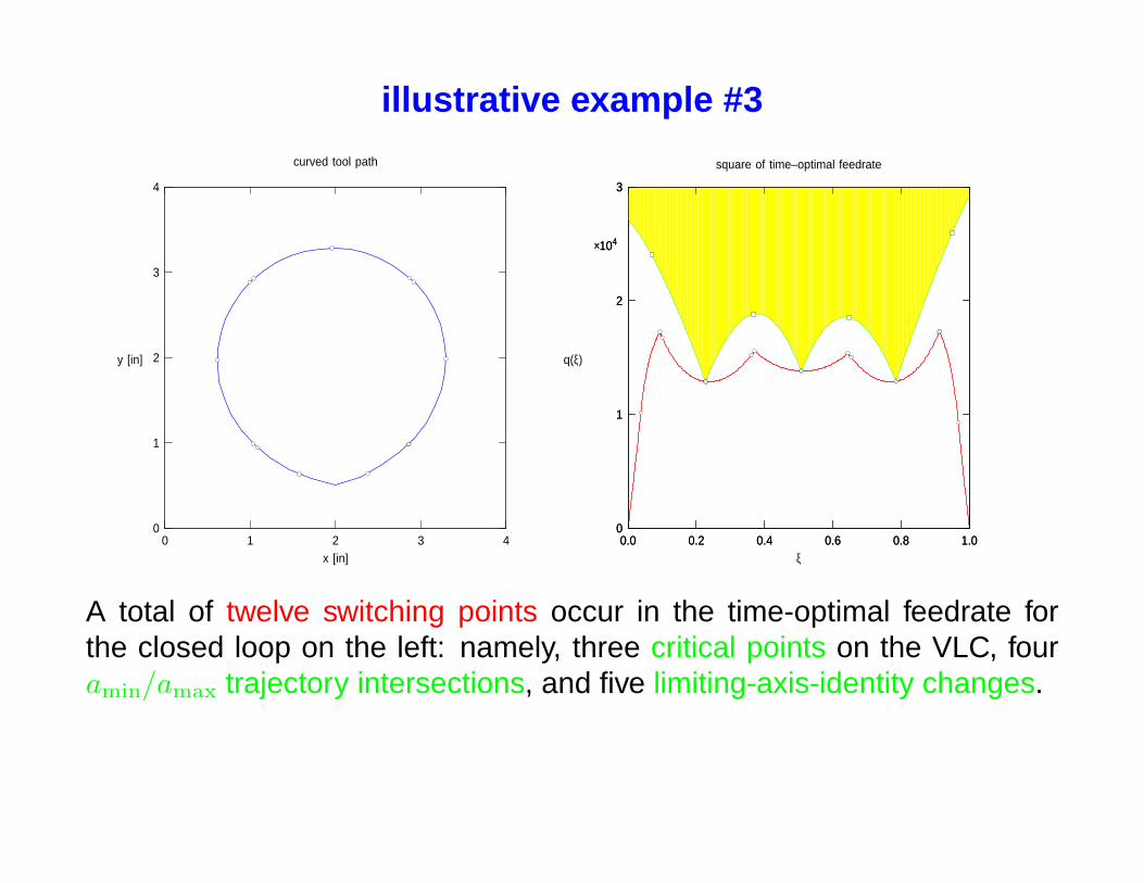
A total of twelve switching points occur in the time-optimal feedrate forthe closed loop on the left: namely, three critical points on the VLC, fouramin/amax trajectory intersections, and five limiting-axis-identity changes.


0.0 0.2 0.4 0.6 0.8 1.00

1

2

3

4

5

×104

0.0 0.2 0.4 0.6 0.8 1.00

1

2

3

4

5

×104

ξ

q(ξ)


0 2 4 6 8 100

2

4

6

8

10

curved tool path

x [in]

y [in]

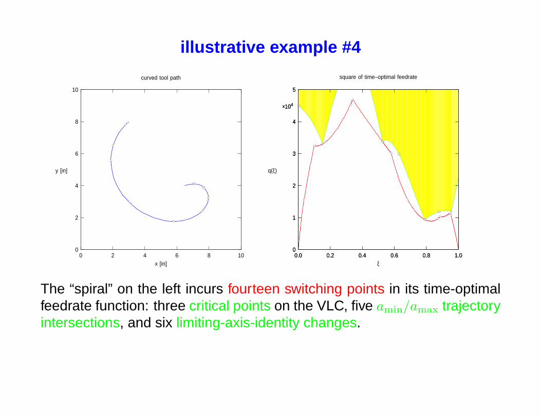
The “spiral” on the left incurs fourteen switching points in its time-optimalfeedrate function: three critical points on the VLC, five amin/amax trajectoryintersections, and six limiting-axis-identity changes.

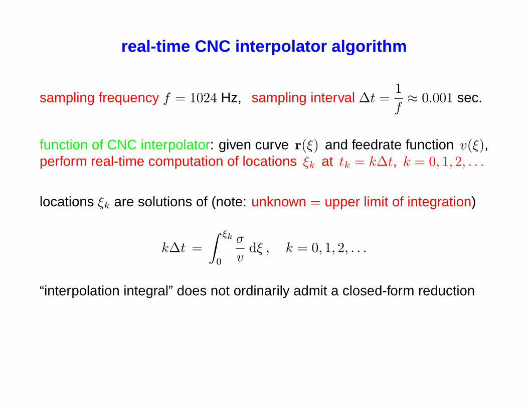
real-time CNC interpolator algorithm

sampling frequency f = 1024 Hz, sampling interval ∆t =1f≈ 0.001 sec.

function of CNC interpolator: given curve r(ξ) and feedrate function v(ξ),perform real-time computation of locations ξk at tk = k∆t, k = 0, 1, 2, . . .

locations ξk are solutions of (note: unknown = upper limit of integration)

k∆t =∫ ξk

0

σ

vdξ , k = 0, 1, 2, . . .

“interpolation integral” does not ordinarily admit a closed-form reduction

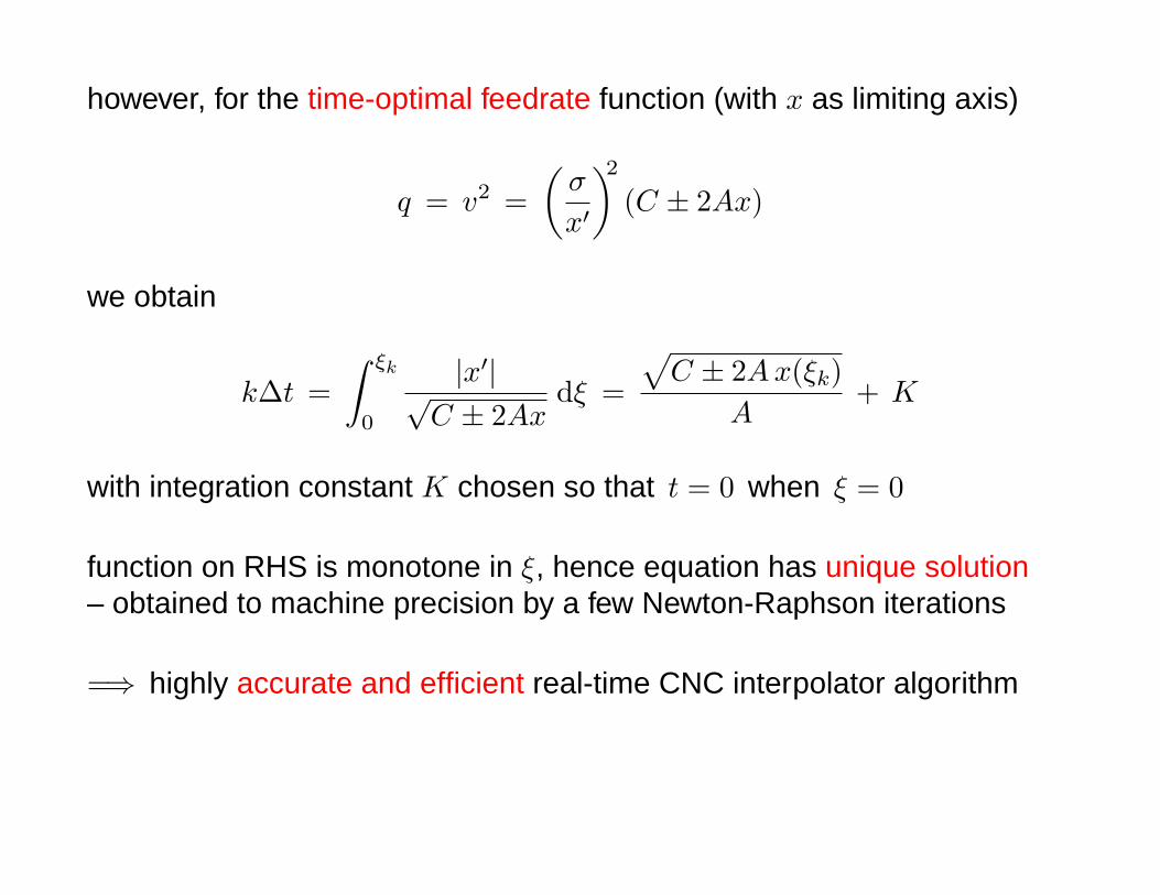
however, for the time-optimal feedrate function (with x as limiting axis)

q = v2 =(

σ

x′

)2

(C ± 2Ax)

we obtain

k∆t =∫ ξk

0

|x′|√C ± 2Ax

dξ =

√C ± 2A x(ξk)

A+ K

with integration constant K chosen so that t = 0 when ξ = 0

function on RHS is monotone in ξ, hence equation has unique solution– obtained to machine precision by a few Newton-Raphson iterations

=⇒ highly accurate and efficient real-time CNC interpolator algorithm

test run data from CNC machine

–2 0 2 4 6 86

8

10

12

14

16

x [in]

y [in

]

0.0 0.2 0.4 0.6 0.8 1.00

2

4

6

8

×104

0.0 0.2 0.4 0.6 0.8 1.00

2

4

6

8

×104

ξ

q(ξ)

Square of time-optimal feedrate is a piecewise-rational function of ξ withfive switching points (one critical and one tangency point on the VLC, andthree switching points below VLC). Record real-time positional data fromencoders on machine axes – obtain velocity & acceleration components byfirst- and second-order differencing. A = 104 in/min2 acceleration bound.

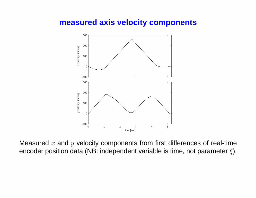
measured axis velocity components

–100

0

100

200

300

x ve

loci

ty [in

/min

]

0 1 2 3 4 5–100

0

100

200

300

time [sec]

y ve

loci

ty [in

/min

]

Measured x and y velocity components from first differences of real-timeencoder position data (NB: independent variable is time, not parameter ξ).

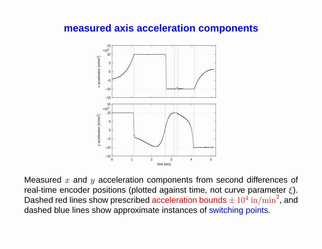
measured axis acceleration components

–15

–10

–5

0

5

10

15

×103

x ac

cele

ratio

n [in

/min

2 ]

0 1 2 3 4 5–15

–10

–5

0

5

10

15

×103

time [sec]

y ac

cele

ratio

n [in

/min

2 ]

Measured x and y acceleration components from second differences ofreal-time encoder positions (plotted against time, not curve parameter ξ).Dashed red lines show prescribed acceleration bounds ± 104 in/min2, anddashed blue lines show approximate instances of switching points.

closure

• for Cartesian machines with independent axis acceleration bounds,an essentially exact piecewise-rational solution for the time-optimal“bang-bang” feedrate can be computed

• optimal feedrate admits accurate & efficient real-time interpolator,based on analytic reduction of the interpolation integral

• a number of errors & inconsistencies exist in the robotics literatureon time-optimal motion along curved paths

• formulate generalizations to systems constrained by axis velocity,as well as acceleration, bounds

• explore automatic smoothing of slope discontinuities in optimalfeedrate function, to obtain smooth (C2) “near-optimal” motions

“science and poetry”

Trace science then, with modesty thy guide;First strip off all her equipage of pride,Deduct what is but vanity, or dress,Or learning’s luxury, or idleness;Or tricks to show the stretch of human brain,Mere curious pleasure, or ingenious pain:Expunge the whole, or lop th’excrescent partsOf all, our vices have created arts:Then see how little the remaining sum,Which served the past, and must the times to come!

Alexander Pope (1688-1744), Essay on Man

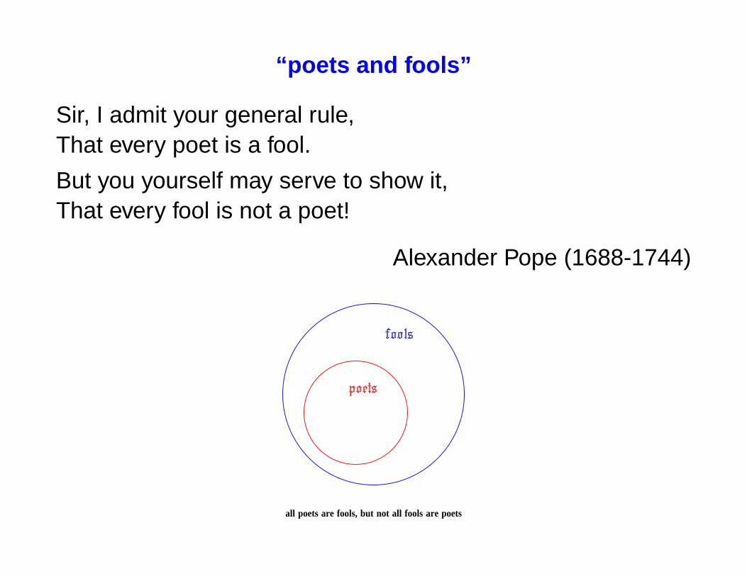
“poets and fools”

Sir, I admit your general rule,That every poet is a fool.

But you yourself may serve to show it,That every fool is not a poet!

Alexander Pope (1688-1744)

all poets are fools, but not all fools are poets

Documents

Algorithms for time-optimal control of CNC machines along