Embed Size (px)
Citation preview
JID:JDA AID:554 /FLA [m3G; v 1.130; Prn:27/03/2014; 8:21] P.1 (1-25)
Journal of Discrete Algorithms ••• (••••) •••–•••
Contents lists available at ScienceDirect
Journal of Discrete Algorithms
www.elsevier.com/locate/jda
Algorithms for topology-free and alignment network queries
Ron Y. Pinter, Meirav Zehavi ∗
Department of Computer Science, Technion, Haifa 32000, Israel
a r t i c l e i n f o a b s t r a c t
Article history:Received 12 November 2012Received in revised form 29 November 2013Accepted 10 March 2014Available online xxxx
Keywords:Topology-free network queryAlignment network queryComputational biologyParameterized algorithmSubgraph homeomorphism
In this article we address two pattern matching problems which have importantapplications to bioinformatics. First we address the topology-free network query problem:Given a set of labels L, a multiset P of labels from L, a graph H = (V H , E H ) anda function LabelH : V H → 2L , we need to find a subtree S of H which is an occurrenceof P . We provide a parameterized algorithm with parameter k = |P | that runs in timeO ∗(2k) and whose space complexity is polynomial. We also consider three variants ofthis problem. Then we address the alignment network query problem: Given two labeledgraphs P and H , we need to find a subgraph S of H whose alignment with P is thebest among all such subgraphs. We present two algorithms for cases in which P andH belong to certain families of DAGs. Their running times are polynomial and they areless restrictive than algorithms that are available today for alignment network queries.Topology-free and alignment network queries provide means to study the function andevolution of biological networks, and today, with the increasing amount of knowledgeregarding biological networks, they are extremely relevant.
© 2014 Elsevier B.V. All rights reserved.
1. Introduction
Performing topology-free and alignment network queries is an important problem in the analysis of biological networks.Such queries provide means to study their function and evolution. In comparison, similar queries for sequences have beenstudied and used extensively for the past 30 years. Today, with the increasing amount of knowledge we have regardingbiological networks, they are extremely relevant for them as well.
In both problems we are given a pattern P and a host graph H , and we need to find a subgraph S of H which resem-bles P . Furthermore, in both problems P and H have labels which we consider when measuring the similarity between Pand the subgraphs of H .
However, there is one significant difference between them: A topology-free network query does not assume we knowthe topology of P and therefore requires only the connectivity of the solution, while an alignment network query assumessuch knowledge and therefore requires resemblance between the topology of P and the solution. Another difference is thatin the optimization version of the topology-free network query problem we consider the sum of the weights of the edgesof the solution, while in the alignment network query problem we are interested in maximizing the similarity between thenodes of P and the solution. This is mostly a result of the uncertainty concerning the existence of many edges in biologicalnetworks that are more suitable for topology-free network queries.
* Corresponding author.E-mail addresses: [email protected] (R.Y. Pinter), [email protected] (M. Zehavi).
http://dx.doi.org/10.1016/j.jda.2014.03.0021570-8667/© 2014 Elsevier B.V. All rights reserved.
JID:JDA AID:554 /FLA [m3G; v 1.130; Prn:27/03/2014; 8:21] P.2 (1-25)
2 R.Y. Pinter, M. Zehavi / Journal of Discrete Algorithms ••• (••••) •••–•••
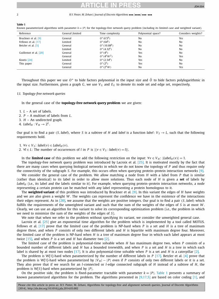
Table 1Known parameterized algorithms with parameter k = |P | for the topology-free network query problem (including its limited case and weighted variant).
Reference General\limited Time complexity Polynomial space? Considers weights?
Bruckner et al. [9] General O ∗(k!3k) No YesFellows et al. [17] Limited O ∗(64k) No NoBetzler et al. [5] General O ∗(10.88k) No No
Limited O ∗(4.32k) No NoGuillemot et al. [20] General O ∗(4k) Yes No
General O ∗(4k W 2) No YesKoutis [24] Limited O ∗(2.54k) Yes NoThis paper General O ∗(2k) Yes No
General O ∗(2k W ) No Yes
Throughout this paper we use O ∗ to hide factors polynomial in the input size and O to hide factors polylogarithmic inthe input size. Furthermore, given a graph G , we use V G and EG to denote its node set and edge set, respectively.
1.1. Topology-free network queries
In the general case of the topology-free network query problem we are given:
1. L – A set of labels.2. P – A multiset of labels from L.3. H – An undirected graph.4. LabelH : V H → 2L .
Our goal is to find a pair (S, label), where S is a subtree of H and label is a function label : V S → L, such that the followingrequirements hold.
1. ∀v ∈ V S : label(v) ∈ LabelH (v).2. ∀l ∈ L: The number of occurrences of l in P is |{v ∈ V S : label(v) = l}|.
In the limited case of this problem we add the following restriction on the input: ∀v ∈ V H : |LabelH (v)| = 1.The topology-free network query problem was introduced by Lacroix et al. [25]. It is motivated mostly by the fact that
there are many cases when querying biological networks in which we do not know the topology of P and thus require onlythe connectivity of the subgraph S . For example, this occurs often when querying protein–protein interaction networks [9].
We consider the general case of the problem. We allow matching a node from H with a label from P that is similar(rather than identical) to its label in order to allow more solutions. Thus each node of H is given a set of labels byLabelH (i.e., its label and the labels similar to it). For example, when querying protein–protein interaction networks, a noderepresenting a certain protein can be matched with any label representing a protein homologous to it.
The weighted variant of this problem was introduced by Bruckner et al. [9]. In this variant the edges of H have weightsand we are also given a weight W . The weights can represent the confidence we have in the existence of the interactionstheir edges represent. As in [20], we assume that the weights are positive integers. Our goal is to find a pair (S, label) whichfulfills the requirements of the unweighted variant and such that the sum of the weights of the edges of S is at most W .Clearly, we can use an algorithm for this variant to solve its corresponding optimization problem (i.e., the problem in whichwe need to minimize the sum of the weights of the edges of S).
We note that when we refer to the problem without specifying its variant, we consider the unweighted general case.Lacroix et al. [25] give an exponential time algorithm for the problem which is implemented by a tool called MOTUS.
Fellows et al. [17] prove that the limited case of the problem is NP-hard when P is a set and H is a tree of maximumdegree three, and when P consists of only two different labels and H is bipartite with maximum degree four. Moreover,the limited case of the problem is NP-hard when H is a tree of maximum degree four in which each label appears at mosttwice [15], and when P is a set and H has diameter two [2].
The limited case of the problem is polynomial-time solvable when H has maximum degree two, when P consists of abounded number of different labels and H has a bounded treewidth, and when P is a set and H is a tree in which eachlabel is shared by at most two nodes [17]. It is also polynomial-time solvable when P is a set and H is a caterpillar [2].
The problem is W[1]-hard when parameterized by the number of different labels in P [17]. Betzler et al. [4] prove thatthe problem is W[1]-hard when parameterized by |V H | − |P | even if P consists of only two different labels or it is a set.They also prove that if we search for an l-connected or l-edge connected subgraph of H instead of a subtree of H , theproblem is W[1]-hard when parameterized by |P |.
On the positive side, the problem is fixed-parameter tractable with parameter k = |P |. Table 1 presents a summary ofknown parameterized algorithms for the problem. The algorithms presented in [9,17,5] are based on color coding [1], and
JID:JDA AID:554 /FLA [m3G; v 1.130; Prn:27/03/2014; 8:21] P.3 (1-25)
R.Y. Pinter, M. Zehavi / Journal of Discrete Algorithms ••• (••••) •••–••• 3
the algorithms presented in [20,24] are based on reductions to the multilinear detection problem [23]. Our algorithms arebased on the algebraic framework of Björklund et al. [6].
We also consider a variant of the problem where we can delete and insert labels to P , and another variant where thesolution may not be connected (known as the min connected components problem). These variants were introduced byBruckner et al. [9] and Dondi et al. [14], respectively.
Remark. During the time in which this paper was under review, Björklund et al. [7] presented algorithms similar to ouralgorithms for the topology-free network query problem and its variant that allows deleting and inserting labels.
1.2. Alignment network queries
When we refer to alignment network queries, we consider node labeled graphs. We use lv to denote the label of a nodev , � is a label-to-label similarity score, and δ is a function specifying for each label l the non-positive cost of deletinga node whose label is l. Given �, δ, a pattern graph P and a host graph H s.t. |P | � |H |, the objective of an alignmentnetwork query is to find a subgraph S of H whose alignment with P is the best among all such subgraphs, considering thetopologies and the similarity (rather than identity) between the node labels of the graphs.
Subgraph isomorphism is the basis for matching topologies by alignment network queries. It is NP-hard even if P is asimple path and H is a general graph, or P is a forest and H is a tree [19]. Given a family of DAGs (i.e., Directed AcyclicGraphs) F , denote by Fund the family of graphs consisting of the underlying undirected graphs of the graphs in F . Usingedge subdivision, it is easy to prove that if subgraph isomorphism is NP-hard for Fund, it is also NP-hard for F . On the
positive side, it is solvable in time O (|V P |1.5|V H |
log |V P | ) for trees [34].In biological networks, certain nodes have been deleted or inserted during evolution, a fact that must be considered by
an alignment network query. Deletions in P can be interpreted as insertions in H and vice versa. Thus considering deletionsin both graphs is equal to considering deletions and insertions in both graphs.
Homeomorphism is a variant of isomorphism that allows deleting nodes whose degrees are two. After a node is deleted,its neighbors are connected. In directed graphs each deleted node must have one ingoing neighbor and one outgoing neigh-bor, and the inserted edge is directed from the ingoing neighbor to the outgoing neighbor. The subgraph homeomorphismproblem is NP-hard [26]. We note that the choice of such deletions has a biological reason (see Section 3.6).
Pinter et al. [30] limit P and H to trees, allow deletions only from H , assume the same deletion cost c ∈ R−0 for all
nodes, and define the following score.
Definition 1. Let c ∈ R−0 . Also let P and S H be two trees s.t. there exists a homeomorphism preserving mapping M from P
to S H which matches all the nodes of P . The ALSH (i.e., Approximate Labeled Subtree Homeomorphism) score of such Mis
ALSH(M) = c · (|V S H | − |V P |) +∑
v∈V P
�[lM(v), lv ]
Definition 2. Given �, c ∈R−0 , and two trees P and H , the ALSH problem is to find a homeomorphism preserving mapping
M from P to a subgraph S H of H which matches all the nodes of P and maximizes the ALSH score.
Pinter et al. [30] give an O (|V P ||V H |(|V P | + log |V H |)) time algorithm for the ALSH problem, which performs in timeO (|V P ||V H |( |V P |
log |V P | + log |V H |)) when the number of labels is bounded. We refer to this algorithm as the ALSH algorithm.Given pairs of nodes which must be matched in the alignment (each pair contains a node from P and a node from H),Lozano et al. [27] show how to achieve better performance for a family of algorithms which includes the ALSH algorithmand the algorithm we present in Section 3.2.
A multisource tree is a directed graph whose underlying undirected graph is a tree. The adaption of the ALSH problemand algorithm to multisource trees and results of using the algorithm to perform inter-species and intra-species alignmentsof metabolic pathways appear in [31]. This algorithm was also used in a pathway evolution study [28].
NetGrep [3] allows P and H to have general topologies. It has an exponential running time and is efficient only for verysmall queries. Cheng et al. [12] allow H to have a general topology, and use homomorphism instead of homeomorphism toprovide a simple polynomial time algorithm. However, allowing different nodes in P to be mapped to the same node in His undesirable.
Another approach, based on color coding [1], enables H to have a general topology. The sum of |V P | and the numberof deletions from H is bounded to k to provide parameterized algorithms with parameter k. This approach is used inQPath [36], which performs linear path queries in time O ∗((2e)k). QNet [35] improves QPath, allowing P to be a boundedtreewidth graph. It runs in time O ∗((3e)k|V H |t+1), where t is the treewidth of P . PADA1 [8] is an alternative to QNet whichbounds the size of the feedback vertex set of P instead of its treewidth. It runs in time O ∗((3e)k|V H ||F |), where |F | is thesize of the feedback vertex set of P . The space complexities of these algorithms have an exponential dependency on k.
JID:JDA AID:554 /FLA [m3G; v 1.130; Prn:27/03/2014; 8:21] P.4 (1-25)
4 R.Y. Pinter, M. Zehavi / Journal of Discrete Algorithms ••• (••••) •••–•••
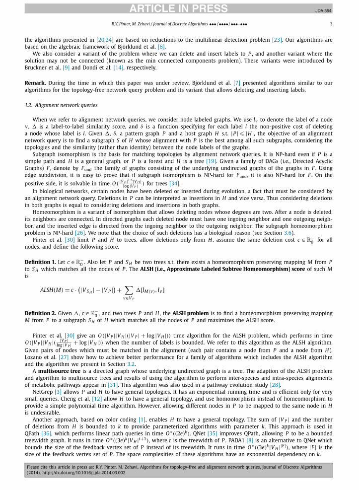
Fig. 1. An illustration used in explaining the definitions given in Sections 2.1 and 2.2. Assume that the labels and neighbors of each node are orderedaccording to the order between their indexes (e.g., N1(v5) = v3 and N2(v5) = v6).
Hüffner et al. [22] show how to reduce the running time of QPath to O ∗(4.32k), and give several practical improvementsto color coding. Scott et al. [33] improve the running time of QPath when each node of P has an additional label whichrestricts the set of nodes of H with whom it can be matched. They also extend QPath to two-terminal series-parallel graphs.
We consider topologies more general than multisource trees, deletions from both P and H and a more flexible deletionsscoring scheme. We use homeomorphism and do not bound P or the number of deletions. Our algorithms have polynomialrunning times and are based on dynamic programming, finding disjoint paths in graphs and maximum weight matchingcomputations.
2. Algorithms for topology-free network queries
Our algorithms are based on the algebraic framework of Björklund et al. [6].We express our parameterized problem by associating monomials with potential solutions. Each feasible solution is
associated with a unique monomial, and each monomial which is not associated with a feasible solution is associated withan even number of different potential solutions. Having a polynomial which is the sum of the monomials associated withpotential solutions, we need to determine whether it has a monomial whose coefficient is odd.
First we consider the unweighted general case of the topology-free network query problem. In Sections 2.1 and 2.2 wedefine the potential solutions. Then, in Sections 2.3 and 2.4, we associate them with monomials and consider the polynomialwhich is the sum of these monomials. Section 2.5 presents the algorithm, and the last three sections concern three variantsof the problem.
Throughout this section we denote |P | by k.
2.1. Potential topologies
Given a rooted tree S , we denote its root by root(S).We intend to traverse H in order to find a solution by using the following approach: If the current node in which we
are located is v , we try to extend some of our partial solutions by using its neighbors. Thus we may visit some nodes morethan once. We use a rooted tree to represent our traversal, where its root corresponds to the node from where we havestarted it. The two following definitions concern this rooted tree.
Definition 3. Given a rooted tree S , a function match : V S → V H , s ∈ V H and an integer t , we say that (S,match) is an(s, t)-potential topology if
1. match(root(S)) = s.2. |V S | = t .3. If {v, u} ∈ E S , then {match(v),match(u)} ∈ E H .4. If v and u are different nodes in S which have the same father, then match(v) �= match(u).
For example, in Fig. 1, (S,match1) and (S,match2) are (v3,5)-potential topologies.

JID:JDA AID:554 /FLA [m3G; v 1.130; Prn:27/03/2014; 8:21] P.5 (1-25)
R.Y. Pinter, M. Zehavi / Journal of Discrete Algorithms ••• (••••) •••–••• 5
Definition 4. Given an (s, t)-potential topology (S,match), its embedding, denoted by EMB(S, match), is a subgraph G of Hwhich is defined as follows:
• V G = {v ∈ V H : ∃u ∈ V S s.t. match(u) = v}.• EG = {{u, v} ∈ E H : ∃{w, p} ∈ E S s.t. {match(w),match(p)} = {u, v}}.
Examples for this definition are given in Fig. 1, illustrating EMB(S,match1) and EMB(S,match2).The following observation follows immediately from Definitions 3 and 4.
Observation 1. Let (S,match) be an (s, t)-potential topology. There are no two nodes in S which match maps to the same node iff|V EMB(S,match)| = t. Moreover, if |V EMB(S,match)| = t, then EMB(S,match) is a tree.
2.2. Potential solutions
Roughly speaking, a potential solution describes a traversal of H in which we label each traversed node v ∈ V H by usinga label from LabelH (v). More precisely, it consists of a potential topology (S,match) (describing the traversal of H) and afunction that assigns a label to each node v ∈ V S from LabelH (match(v)) (indicating the labels of the traversed nodes).
Formally, our potential solutions are defined as follows.
Definition 5. Given an (s, t)-potential topology (S,match) and a function label : V S → L, we say that (S,match, label) is an(s, t)-potential solution if ∀v ∈ V S : label(v) ∈ LabelH (match(v)).
For example, in Fig. 1, (S,matchi, label j) is a (v3,5)-potential solution for all i, j ∈ {1,2}.
Definition 6. We say that an (s, t)-potential solution (S,match, label) is bijectively labeled if label is bijective.
For example, in Fig. 1, (S,match1, label2) and (S,match2, label2) are bijectively labeled.We next determine which potential solutions are feasible solutions. First we show that we can assume WLOG that P = L.Suppose that L contains labels which do not appear in P . We can delete them from L and from the sets assigned by
LabelH , and get that a subtree of H is a solution to the original instance iff it is a solution to the new one.Now suppose l is a label which appears nl > 1 times in P . We can replace l with nl new labels l1, l2, . . . , lnl as follows.
1. Remove l from L and insert each of the new labels.2. Remove the occurrences of l from P and insert each of the new labels once.3. Replace LabelH with the following function Label′H : V H → 2L .
Label′H (v) ={
(LabelH (v) \ {l}) ∪ {l1, l2, . . . , lnl } if l ∈ LabelH (v)
LabelH (v) otherwise
Again we get that a subtree of H is a solution to the original instance iff it is a solution to the new one. We can repeatthis process for each label which appears more than once in P , and thus we make the following assumption.
Assumption 1. We assume WLOG that P = L.
Given an instance (L, H, LabelH ) of the problem (note that P = L) and a node s ∈ V H , denote by Bi jL,H,LabelH ,s theset of all bijectively labeled (s,k)-potential solutions, and by BijTree
L,H,LabelH ,s the set of all bijectively labeled (s,k)-potential
solutions whose embeddings have k nodes. When L, H, LabelH and s are clear from context, we write only Bi j and Bi jTree .For example, in Fig. 1, (S,match1, label2) ∈ BijP ,H,LabelH ,v3
\ Bi jTree and (S,match2, label2) ∈ Bi jTreeP ,H,LabelH ,v3
.
Suppose that (S,m, l) ∈ BijTreeL,H,LabelH ,s . By Observation 1, EMB(S,m) is a tree on k nodes and m−1 is well defined. We get
that l ◦ m−1 : V EMB(S,m) → L fulfills the requirement [∀v ∈ V EMB(S,m) : l ◦ m−1(v) ∈ LabelH (v)] and uses each label of L once.Thus we get the following observation.
Observation 2. Given (S,m, l) ∈ BijTreeL,H,LabelH ,s , (EMB(S,m), l ◦ m−1) is a solution to the instance (L, H, LabelH ) of the problem.
Furthermore, we have the following simple observation.
Observation 3. Let (S∗, label∗) be a solution to an instance (L, H, LabelH ) of the problem that contains a node s. Then there is a tuple(S,match, label) ∈ BijTree
L,H,LabelH ,s s.t. EMB(S) = S∗ and label∗ ≡ label ◦ match−1 .
JID:JDA AID:554 /FLA [m3G; v 1.130; Prn:27/03/2014; 8:21] P.6 (1-25)
6 R.Y. Pinter, M. Zehavi / Journal of Discrete Algorithms ••• (••••) •••–•••
2.3. The monomials associated with potential solutions
We introduce one indeterminate xe for each edge e ∈ E H , and one indeterminate yv,l for each pair of node v ∈ V H andlabel l ∈ L. We rename them arbitrarily as z1, z2, . . . , z|E H |+k|V H | . For an indeterminate of the type xe (resp. yv,l), index(e)(resp. index(v, l)) denotes the index it received in this ordering.
First we associate a monomial with each potential solution.
Definition 7. The monomial of an (s, t)-potential solution (S,match, label) is
m(S,match, label) =∏
{v,u}∈E S
x{match(v),match(u)}∏
v∈V S
ymatch(v),label(v)
For example, in Fig. 1, the monomials associated with (S,matchi, label j) for i, j ∈ {1,2} are:
• i = 1, j = 1: x{v3,v4}x2{v3,v6}x{v4,v6} y2v3,l4
y2v4,l2
yv6,l5 .
• i = 1, j = 2: x{v3,v4}x2{v3,v6}x{v4,v6} yv3,l1 yv3,l4 yv4,l2 yv4,l3 yv6,l5 .• i = 2, j = 1: x{v2,v3}x{v3,v6}x{v4,v6}x{v5,v6} yv2,l2 yv3,l4 yv4,l2 yv5,l4 yv6,l5 .• i = 2, j = 2: x{v2,v3}x{v3,v6}x{v4,v6}x{v5,v6} yv2,l2 yv3,l1 yv4,l3 yv5,l4 yv6,l5 .
On the one hand, we have the following observation.
Observation 4. Let e be an element in BijTreeL,H,LabelH ,s . Then, there is no element e′ �= e in BijL,H,LabelH ,s which has the same monomial
as e.
On the other hand, for Bij \ Bi jTree we have the following lemma.
Lemma 1. There is a fixed-point-free involution (i.e., a permutation that is its own inverse) f : BijL,H,LabelH ,s \ BijTree → Bij \ BijTree s.t.
m(S,m, l) = m( f (S,m, l)) for all (S,m, l) ∈ Bi j \ BijTree.
Proof. Select arbitrarily an order < on the labels in L. Given a,b, c,d ∈ L, (a,b) < (c,d) iff a < c or (a = c ∧ b < d).Let (S,m, l) be an element of Bij \ BijTree and denote:
1. M S,m,l = {{v, u}: v, u ∈ V S , v �= u,m(v) = m(u)}.2. SwapS,m,l = argmin{v,u}∈M(S,m,l){(min{l(v), l(u)}, max{l(v), l(u)})}.
For example, for (S,match1, label2) as in Fig. 1, we get that M S,match1,label2 = {{u1, u4}, {u3, u5}} and SwapS,match1,label2 ={u1, u4}.
By Observation 1, M S,m,l �= ∅. Since for each {v, u} ∈ M S,m,l we have a different (min{l(v), l(u)}, max{l(v), l(u)}), SwapS,m,lis well defined.
Denote {v∗, u∗} = SwapS,m,l . We define lS,m,l as l except that lS,m,l(v∗) = l(u∗) and lS,m,l(u∗) = l(v∗). Since m(v∗) = m(u∗)and (S,m, l) ∈ Bij \ BijTree , we have that ∀v ∈ V S : lS,m,l(v) ∈ LabelH (m(v)). Therefore (S,m, lS,m,l) ∈ Bij \ BijTree .
We define f (S,m, l) = (S,m, lS,m,l). Clearly m(S,m, l) = m( f (S,m, l)). Similarly we define f for each element in Bij\BijTree
to get a function f : Bij \ BijTree → Bij \ BijTree .Denote l′ = lS,m,l , {v∗∗, u∗∗} = SwapS,m,l′ and l′′ = lS,m,l′ . Therefore e′ = (S,m, l′) = f (e) and e′′ = (S,m, l′′) = f ( f (e)). We
need to prove that e �= e′ and e = e′′ .We prove that e �= e′ by showing that there is no function g : V S → V S s.t.
1. ∀v ∈ V S : m(v) = m(g(v)) ∧ l(v) = l′(g(v)).2. ∀v, u ∈ V S s.t. v is an ancestor of u in S: g(v) is an ancestor of g(u) in S.
By our definition of l′ and since l is bijective, the only g which fulfills the first requirement is defined as follows:
g(v) =⎧⎨⎩
u∗ if v = v∗v∗ if v = u∗v otherwise
If v∗ and u∗ do not have the same father, g does not fulfill the second requirement. However, since m(v∗) = m(u∗) and(S,m) is an (s,k)-potential topology, we get that v∗ and u∗ cannot have the same father and thus e �= e′ .
In order to prove that e = e′′ , it is enough to show that l ≡ l′′ . This follows by observing that {v∗, u∗} = {v∗∗, u∗∗}. �Now we sum the monomials that are associated with bijectively labeled (s,k)-potential solutions:
JID:JDA AID:554 /FLA [m3G; v 1.130; Prn:27/03/2014; 8:21] P.7 (1-25)
R.Y. Pinter, M. Zehavi / Journal of Discrete Algorithms ••• (••••) •••–••• 7
Definition 8. Given an instance (L, H, LabelH ) of the problem and a node s of H , their polynomial is
POLL,H,LabelH ,s(z1, z2, . . . , z|E H |+k|V H |) =∑
(S,match,label)∈BijL,H,LabelH ,s
m(S,match, label).
Observations 2, 3 and 4 and Lemma 1 imply the following lemma.
Lemma 2. Let s ∈ V H . An instance (L, H, LabelH ) of the problem has a solution which contains s iff POLL,H,LabelH ,s has a monomialwith an odd coefficient.
Proof. First suppose that (L, H, LabelH ) has a solution which contains s. By Observation 3, there is e ∈ BijTreeL,H,LabelH ,s . By
Observation 4, there is no element e′ �= e in BijL,H,LabelH ,s which has the same monomial as e. We get that POLL,H,LabelH ,s hasa monomial with coefficient 1.
Now suppose that POLL,H,LabelH ,s has a monomial with an odd coefficient. By Lemma 1, there is e ∈ BijTreeL,H,LabelH ,s . Then,
by Observation 2, we get that there is a solution to (L, H, LabelH ) which contains s. �2.4. Evaluating POLL,H,LabelH ,s
We evaluate the polynomial over the finite field Fq (i.e., the finite field of order q), where q = 2�log(3(2k−1)|V H |)� . Sincethis field has characteristic 2, we get the following corollary to Lemma 2.
Corollary 1. Let s ∈ V H . An instance (L, H, LabelH ) of the problem has a solution which contains s iff POLL,H,LabelH ,s is a nonzeropolynomial.
The following lemma is proved in [13] and [32].
Lemma 3. Let p(x1, x2, . . . , xn) be a nonzero polynomial of total degree at most d over the finite field F . Then, for a1,a2, . . . ,an ∈ Fselected independently and uniformly at random: Pr(p(a1,a2, . . . ,an) �= 0) � 1 − d/|F |.
Note that the degree of POLL,H,LabelH ,s is at most 2k − 1. Using Corollary 1 and Lemma 3, we get the following lemma.
Lemma 4. Suppose s ∈ V H , and a1,a2, . . . ,a|E H |+k|V H | ∈ Fq are selected independently and uniformly at random. If the in-stance (L, H, LabelH ) has a solution which contains s, then Pr(POLL,H,LabelH ,s(a1,a2, . . . ,a|E H |+k|V H |) �= 0) � 1 − 1
3|V H | . OtherwisePOLL,H,LabelH ,s(a1,a2, . . . ,a|E H |+k|V H |) = 0.
Given A ⊆ L, let L[A, s] denote the set of (s,k)-potential solutions that do not use labels from A. The principle ofinclusion–exclusion implies the following observation, and the fact that the polynomial is evaluated over a field of charac-teristic 2 implies its following corollary.
Observation 5.
POLL,H,LabelH ,s(z1, z2, . . . , z|E H |+k|V H |) =∑A⊆L
(−1)|A| ∑(S,match,label)∈L[A,s]
m(S,match, label).
Corollary 2.
POLL,H,LabelH ,s(z1, z2, . . . , z|E H |+k|V H |) =∑A⊆L
∑(S,match,label)∈L[A,s]
m(S,match, label).
Select A ⊆ L and a1,a2, . . . ,a|E H |+k|V H | ∈ Fq arbitrarily. Next we present a procedure EVAL(L, H, LabelH , A,a1,a2, . . . ,
a|E H |+k|V H |) for evaluating the sum∑
(S,match,label)∈L[A,v] m(S,match, label) for all v ∈ V H in polynomial time where ∀1 � i �|E H | + k|V H |,ai is assigned to zi .
For each v ∈ V H , we order its neighbors in H arbitrarily and denote them accordingly as N1(v), N2(v), . . . , Nd(v)(v),where d(v) denotes their number.
The next definition will help us enforce condition 4 of Definition 3.
Definition 9. Given v ∈ V H and integers t and i s.t. 1 � t and 0 � i � d(s), we say that a (v, t)-potential solution(S,match, label) is a (v, t, i)-potential solution if root(S) does not have a son u s.t. match(u) = N p(v) for p � i.
JID:JDA AID:554 /FLA [m3G; v 1.130; Prn:27/03/2014; 8:21] P.8 (1-25)
8 R.Y. Pinter, M. Zehavi / Journal of Discrete Algorithms ••• (••••) •••–•••
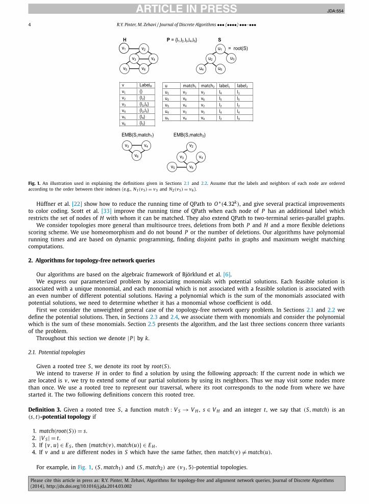
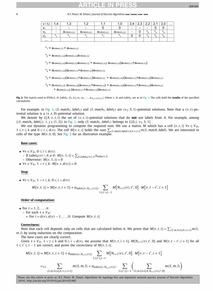
Fig. 2. The matrix used in EVAL(L, H, LabelH , {l3, l5},a1,a2, . . . ,a|E H |+k|V H |), where L, H and LabelH are as in Fig. 1. The cells hold the results of the specifiedcalculations.
For example, in Fig. 1, (S,match1, label1) and (S,match1, label2) are (v3,5,1)-potential solutions. Note that a (v, t)-po-tential solution is a (v, t,0)-potential solution.
We denote by L[A, v, t, i] the set of (v, t, i)-potential solutions that do not use labels from A. For example, among{(S,matchi, label j): i, j ∈ {1,2}} in Fig. 1, only (S,match1, label1) belongs to L[{l1}, v3,5,1].
We use dynamic programming to compute the required sum. We use a matrix M which has a cell [v, t, i] ∀v ∈ V H ,1 � t � k and 0 � i � d(v). The cell M[v, t, i] holds the sum
∑(S,match,label)∈L[A,v,t,i] m(S,match, label). We are interested in
cells of the type M[v,k,0]. See Fig. 2 for an illustrative example.
Base cases:
• ∀v ∈ V H , 0 � i � d(v):– If LabelH (v) \ A �= ∅: M[v,1, i] = ∑
l∈LabelH (v)\A aindex(v,l)– Otherwise: M[v,1, i] = 0
• ∀v ∈ V H , 1 < t � k: M[v, t,d(v)] = 0
Step:
• ∀v ∈ V H , 1 < t � k, 0 � i < d(v):
M[v, t, i] = M[v, t, i + 1] + aindex({v,Ni+1(v)})∑
1�t′�t−1
M[Ni+1(v), t′,0
] · M[v, t − t′, i + 1
]
Order of computation:
• For t = 1,2, . . . ,k:– For each v ∈ V H :
∗ For i = d(v),d(v) − 1, . . . ,0: Compute M[v, t, i]
Correctness:Note that each cell depends only on cells that are calculated before it. We prove that M[v, t, i] = ∑
(S,m,l)∈L[A,v,t,i] m(S,
m, l) by using induction on the computation.The base cases are clearly correct.Given v ∈ V H , 1 < t � k and 0 � i < d(v), we assume that M[v, t, i + 1], M[Ni+1(v), t′,0] and M[v, t − t′, i + 1] for all
1 � t′ � t − 1 are correct, and prove the correctness of M[v, t, i].
M[v, t, i] = M[v, t, i + 1] + aindex({v,Ni+1(v)})∑
1�t′�t−1
M[Ni+1(v), t′,0
] · M[v, t − t′, i + 1
]
=∗1
∑(S,m,l)∈L[A,v,t,i+1]
m(S,m, l) + aindex({v,Ni+1(v)}) ·∑
1�t′�t−1
( ∑(S,m,l)∈L[A,N (v),t′,0]
m(S,m, l)
)
i+1
JID:JDA AID:554 /FLA [m3G; v 1.130; Prn:27/03/2014; 8:21] P.9 (1-25)
R.Y. Pinter, M. Zehavi / Journal of Discrete Algorithms ••• (••••) •••–••• 9
·( ∑
(S,m,l)∈L[A,v,t−t′,i+1]m(S,m, l)
)
=∗2
∑(S,m,l)∈L[A,v,t,i+1]
m(S,m, l) +∑
(S,m,l)∈L[A,v,t,i]s.t.root(S) has a son u for which m(u)=Ni+1(v)
m(S,m, l)
=∑
(S,m,l)∈L[A,v,t,i]m(S,m, l)
*1 – by the induction hypothesis.*2 – by the definitions of L[A, v, t, i], (v, t, i)-potential solutions and their monomials.
Time and space complexities:
The procedure runs in time O (∑
v∈V H
∑1�t�k
∑0�i�d(v) t) = O (|E H |k2). We have O (|E H |k) cells and each requires O (1)
space. Therefore the space complexity is O (|E H |k).
2.5. The algorithm
First we present an algorithm for the decision version of the problem. We use the matrix M of the procedure EVAL (seeSection 2.4), and an array SUM which has a cell for every node of H .
DECIDE(L, H, LabelH ):
1. Select a1,a2, . . . ,a|E H |+k|V H | ∈ Fq independently and uniformly at random.2. Initialize each of the cells of SUM to 0.3. For each A ⊆ L:
(a) Run the procedure EVAL(L, H, LabelH , A,a1,a2, . . . ,a|E H |+k|V H |).(b) For each s ∈ V H : SUM[s] ⇐ SUM[s] + M[s,k,0].
4. Accept iff at least one of the cells of SUM does not hold 0.
Correctness:Lemma 4, Corollary 2 and the correctness of EVAL imply the following lemma.
Lemma 5. Let (L, H, LabelH ) be an instance of the problem. If it has a solution, then the algorithm accepts with probability at least1 − 1
3|V H | . Otherwise the algorithm rejects.
Time and space complexities:By the pseudocode of the algorithm and the time and space complexities of EVAL, the running time of the algorithm is
O (2k|E H |k2) and its space complexity is O (|E H |k).
Using the decision algorithm, we now solve the search version of the problem.
SEARCH(L, H, LabelH ):
1. Initialize H ′ as H .2. For each node v ∈ V H :
(a) Initialize H ′′ as H ′ without v and the edges that are incident to it.(b) If DECIDE(L, H ′′, LabelH ) accepts, assign H ′ ⇐ H ′′ .
3. If |V H ′ | �= k, return NIL.4. Calculate a spanning tree S of H ′ . If such S does not exist (i.e., H ′ is not connected), return NIL.5. Construct a bipartite graph G = (V S , L, E) where E = {{v, l} : l ∈ LabelH (v)}. Calculate a maximum matching M in G . If
its size is not k, return NIL. Else set label : V S → L according to M (i.e., label(v) is the label l with whom v is matchedby M).
6. Return (S, label).
Correctness:Let (L, H, LabelH ) be an instance of the problem. By the pseudocode, if the instance does not have a feasible solution
then the algorithm returns NIL, and if the algorithm returns a solution then it is a feasible solution.Now suppose that the instance has a feasible solution. By the pseudocode and Lemma 5, the probability that the algo-
rithm returns a solution is at least the probability that the decision algorithm answers correctly |V H | times, which is atleast (1 − 1
3|V H | )|V H | � 2/3.
Thus we have the following lemma.

JID:JDA AID:554 /FLA [m3G; v 1.130; Prn:27/03/2014; 8:21] P.10 (1-25)
10 R.Y. Pinter, M. Zehavi / Journal of Discrete Algorithms ••• (••••) •••–•••
Lemma 6. Let (L, H, LabelH ) be an instance of the problem. If it has a solution, then the algorithm returns a feasible solution withprobability at least 2/3. Otherwise the algorithm returns NIL.
Time and space complexities:
We find a spanning tree in Step 4 in time O (k2) by using depth-first search and a maximum matching in Step 5 in timeO (k2.376) [29]. Thus, by the pseudocode and the time and space complexities of the decision algorithm, we have that therunning time of the algorithm is O (2k|E H ||V H |k2) and its space complexity is O (|E H |k).
We have proved the following theorem.
Theorem 1. The general case of the topology-free network query problem can be solved in time O ∗(2k) and polynomial space com-plexity by a randomized algorithm with a constant, one-sided error.
2.6. The weighted variant
Guillemot et al. [20] show how to modify their algorithm for the unweighted case to the weighted case while increasingits running time by O ∗(W 2) and its space complexity by O ∗(W ). Their idea can also be used for our algorithm. We showa different idea which increases the running time of our algorithm by O ∗(W ) and its space complexity by O ∗(W ).
We assume WLOG that the weight of each edge in H is at most W . We add an indeterminate w to which we do notassign values, and perform only one change in the decision algorithm for the unweighted case, which is in the step of theprocedure EVAL. Each cell [v, t, i] of M holds a polynomial in w with coefficients from Fq whose degree is at most W , andwe use the degrees of w to track the weights of its corresponding (v, t, i)-potential solutions.
Step:
• ∀v ∈ V H , 1 < t � k, 0 � i < d(v):
M[v, t, i] = M[v, t, i + 1] + w weight({v,Ni+1(v)})aindex({v,Ni+1(v)})∑
1�t′�t−1
M[Ni+1(v), t′,0
] · M[v, t − t′, i + 1
]
where we omit monomials of the form c · wd where c ∈ Fq and d > W .
In the search algorithm we change Step 4 as follows.
4. Calculate a minimum-weight spanning tree S of H ′ . If such S does not exist or the sum of the weights of its edges ismore than W , return NIL.
The proofs of correctness of the decision and search algorithms are similar to those of the original algorithms. Further-more, their space complexity is clearly O (W |E H |k).
We compute each minimum weight spanning tree in time O (k2) [11]. Each cell in M requires O (k) multiplications ofpolynomials with coefficients from Fq whose degrees are at most W (then we omit the unnecessary monomials in O (W )
time). Each such multiplication can be done in time O (W log W ) [21]. Thus the running time of the decision algorithm isO (2k|E H |k2W log W ) and of the search algorithm it is O (2k|E H ||V H |k2W log W ).
We have proved the following lemma.
Lemma 7. The weighted general case of the topology-free network query problem can be solved in time O ∗(2k W ) and space complexityO ∗(W ) by a randomized algorithm with a constant, one-sided error.
2.7. Allowing deletions and insertions
As we have noted in Section 1.2, in biological networks certain nodes have been deleted or inserted during evolution.Therefore we consider the variant of the problem in which we also have:
• D – A nonnegative integer (D stands for deletions).• I – A nonnegative integer (I stands for insertions).
Our goal is to find a triple (S, U , label) where S is a subtree of H s.t. |V S | � |U |+ I , U ⊆ V S s.t. |U | � k − D , label : U → Land the following requirements hold.
1. ∀v ∈ U : label(v) ∈ LabelH (v).2. ∀l ∈ L: The number of occurrences of l in P is at least |{v ∈ U : label(v) = l}|.
JID:JDA AID:554 /FLA [m3G; v 1.130; Prn:27/03/2014; 8:21] P.11 (1-25)
R.Y. Pinter, M. Zehavi / Journal of Discrete Algorithms ••• (••••) •••–••• 11
We assume WLOG that D � k and I � |V H |. We briefly explain how to modify the algorithm presented in Section 2.5 towork for this variant.
We use the following definition for potential solutions.
Definition 10. Given a (v, t)-potential topology (S,m), U ⊆ V S and l : U → L, (S,m, U , l) is a (v, t, i, j)-potential solution if
1. ∀v ∈ U : l(v) ∈ LabelH (match(v)).2. root(S) does not have a son u s.t. m(u) = Np(v) for p � i.3. |V S | = t + j and |U | = t .
L[A, v, t, i, j] denotes the set of (v, t, i, j)-potential solutions that do not use labels from A.We modify the dynamic programming calculation to track the number of insertions. We use a matrix M which
has a cell [v, t, i, j] for each v ∈ V H , 0 � t � k − D , 0 � i � d(v) and 0 � j � I . The cell M[v, t, i, j] holds the sum∑(S,match,label)∈L[A,v,t,i, j] m(S,match, label).
Base cases:
• ∀v ∈ V H ,0 � i � d(v):– If LabelH (v) \ A �= ∅: M[v,1, i,0] = ∑
l∈LabelH (v)\A aindex(v,l)– Otherwise: M[v,1, i,0] = 0
• ∀v ∈ V H ,0 � i � d(v): M[v,0, i,1] = 1• ∀v ∈ V H , 0 � t � k − D , 0 � j � I s.t. 1 < t + j: M[v, t,d(v), j] = 0
Step:
• ∀v ∈ V H , 0 � t � k − D , 0 � i < d(v), 0 � j � I s.t. 1 < t + j:
M[v, t, i, j] = M[v, t, i + 1, j] + aindex({v,Ni+1(v)}) ·∑
0�t′�t, 0� j′� j s.t. 1�t′+ j′�t+ j−1
M[Ni+1(v), t′,0, j′
]· M
[v, t − t′, i + 1, j − j′
]In the decision algorithm we change Step 3(b) as follows.
3. (b) For each s ∈ V H : SUM[s] ⇐ SUM[s] + ∑0� j�I M[s,k − D,0, j].
In the search algorithm we change Steps 3, 5 and 6 as follows.
3. If |V H ′ | > k − D + I , return NIL.
5. Construct a bipartite graph G = (V S , L, E) where E = {{v, l}: l ∈ LabelH (v)}. Calculate a maximum matching M in G . If|M| < k − D , return NIL. Else set U as the set of matched nodes, and set label : U → L according to M .
6. Return (S, U , label).
The proofs of correctness of the decision and search algorithms are similar to those of the original algorithms. Therunning time is increased by O (I2) and the space complexity by O (I). We have the following lemma.
Lemma 8. The general case of the topology-free network query problem with deletions and insertions can be solved in time O ∗(2k)
and polynomial space complexity by a randomized algorithm with a constant, one-sided error.
2.8. Reduction to the min connected components problem
In the general case of the min connected components problem we have:
1. L – A set of labels.2. P – A multiset of labels from L.3. H – An undirected graph.4. LabelH : V H → 2L .5. c – A positive integer.
Our goal is to find a pair (S, label) where S is a subforest of H of at most c trees, label : V S → L and the followingrequirements hold.

JID:JDA AID:554 /FLA [m3G; v 1.130; Prn:27/03/2014; 8:21] P.12 (1-25)
12 R.Y. Pinter, M. Zehavi / Journal of Discrete Algorithms ••• (••••) •••–•••
1. ∀v ∈ V S : label(v) ∈ LabelH (v).2. ∀l ∈ L: The number of occurrences of l in P is |{v ∈ V S : label(v) = l}|.
In the limited case of this problem we add the following restriction on the input: ∀v ∈ V H : |LabelH (v)| = 1.The min connected components problem was introduced by Dondi et al. [14]. There is a simple reduction from the min
connected components problem to the weighted topology-free network query problem with 0\1 weights by Guillemot etal. [20]: Given L, P , H, LabelH and c, we construct a complete graph H ′ with the same nodes. We assign a weight 0 to theedges of H ′ which appear also in H and 1 to the other edges. We set W = c − 1. The input for the weighted topology-freenetwork query problem is L, P , H ′, LabelH and W .
The algorithms with the previous best running times to the min connected components problem use this reduction andachieve time O ∗(4k) for the general case [20] and time O ∗(2.54k) for the limited case [24]. Using the same reduction, wehave the following lemma.
Lemma 9. The general case of the min connected components problem can be solved in time O ∗(2k) and polynomial space complexityby a randomized algorithm with a constant, one-sided error.
3. Algorithms for alignment network queries
First we present our definitions and the intuition behind them. In particular, we present the SubDAG alignment problem,which is our definition for the alignment network query problem. We then present an algorithm for multisource trees.Afterwards we modify it to work for a certain family of DAGs. In the following two sections we provide the proofs ofcorrectness of the algorithms and analyze their running times. Our algorithms are based on dynamic programming, findingdisjoint paths in graphs and maximum weight matching computations. Finally, we briefly discuss an application of ouralgorithms to the alignment of metabolic pathways.
3.1. Definitions
We start by giving a definition regarding disjoint paths in DAGs, which is followed by an explanation of the intuitionbehind its necessity. We note that dsr stands for distribution, and frb stands for forbidden.
Definition 11. Given a DAG G and a node v ∈ V G , define:
1. dsr(v) = {c ∈ V G : there are two internally node-disjoint paths from v to c}.2. frb(v) = {c ∈ V G : ∃u ∈ V G s.t. there are two internally node-disjoint paths from u to c and v is on exactly one of them}.3. dsr(G) = maxv∈V G |dsr(v)|, frb(G) = maxv∈V G |frb(v)|.4. G is a treelike DAG if dsr(G) and frb(G) are bounded.5. v is a crossroad if ∃u ∈ V G s.t. v ∈ dsr(u).
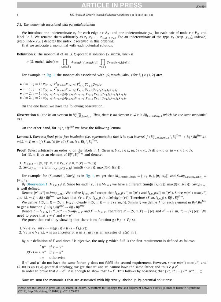
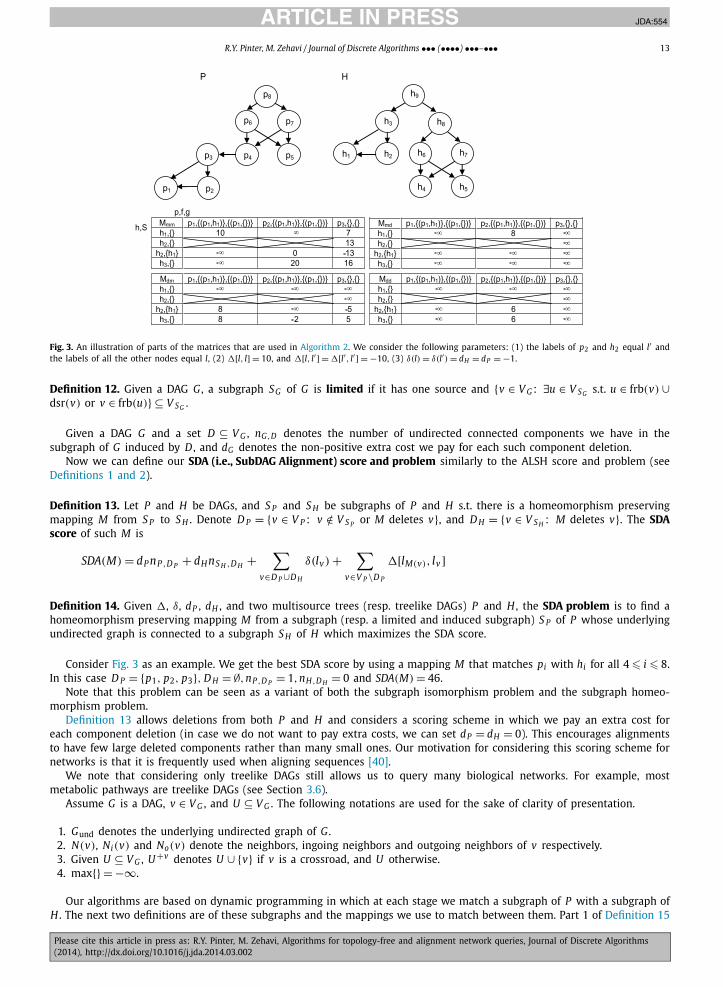
For example, in Fig. 3, the nonempty dsr and frb sets are frb(p2) = dsr(p3) = {p1}, frb(h2) = dsr(h3) = {h1}, frb(p6) =frb(p7) = dsr(p8) = {p4, p5} and frb(h6) = frb(h7) = dsr(h8) = {h4,h5}. We have that frb(P ) = dsr(P ) = frb(H) = dsr(H) = 2,and the crossroads are p1, p4, p5,h1,h4 and h5.
When matching two nodes, we decide how to map the subgraphs of their outgoing neighbors, where a subgraph ofa node is the nodes that are reachable from it and the edges between them. Consider the graphs given in Fig. 3. Whenmatching p8 with h8, we map the subgraphs of p6 and p7 to the subgraphs of h6 and h7. We cannot match a node p∗that belongs to both the subgraphs of p6 and p7 with one node when mapping the subgraph of p6 and with another whenmapping the subgraph of p7, and then construct one mapping from these two mappings (since we need the mapping tomatch each node in the subgraph of p8 with one node of H , and here we match p∗ with two different nodes of H). Thesubgraphs of p6 and p7 must agree on how the crossroads in dsr(p8) are matched with the crossroads in dsr(h8) (e.g.,p4 ∈ dsr(p8) cannot be matched with h4 ∈ dsr(h8) in the subgraph of p6 and with h5 ∈ dsr(h8) in the subgraph of p7).Thus, when matching p8 with h8, we compute how to map the subgraphs of p6 and p7 with the subgraphs of h6 and h7subject to a distribution of dsr(p8) to dsr(h8) (i.e., a function from dsr(p8) to dsr(h8), indicating how to match the nodesin dsr(p8)). Moreover, when matching p6 we are forbidden from deciding how to match the crossroads in frb(p6) (we savethe scores of all such options). Similarly, when matching p7, h6 and h7, we are forbidden from deciding how to matchthe crossroads in their frb sets. Only afterwards, when iterating over each distribution of dsr(p8) to dsr(h8), we make thisdecision.
We use the next definition to limit the subgraphs which are potential solutions (e.g., if a node u is in a potential solution,we assume that each node v that is supposed to distribute it (i.e., u ∈ dsr(v)) and each of the nodes on the paths from v tou (i.e., nodes that have u in their frb sets) are also in the potential solution). This allows us to design an efficient algorithmfor treelike DAGs. We can still delete nodes from such a subgraph, but only if they have one ingoing neighbor and oneoutgoing neighbor in the subgraph. Consider Fig. 3 as an example. If p1 is in a potential solution then so are p2 and p3,and p2 can be deleted.
JID:JDA AID:554 /FLA [m3G; v 1.130; Prn:27/03/2014; 8:21] P.13 (1-25)
R.Y. Pinter, M. Zehavi / Journal of Discrete Algorithms ••• (••••) •••–••• 13
Fig. 3. An illustration of parts of the matrices that are used in Algorithm 2. We consider the following parameters: (1) the labels of p2 and h2 equal l′ andthe labels of all the other nodes equal l, (2) �[l, l] = 10, and �[l, l′] = �[l′, l′] = −10, (3) δ(l) = δ(l′) = dH = dP = −1.
Definition 12. Given a DAG G , a subgraph SG of G is limited if it has one source and {v ∈ V G : ∃u ∈ V SG s.t. u ∈ frb(v) ∪dsr(v) or v ∈ frb(u)} ⊆ V SG .
Given a DAG G and a set D ⊆ V G , nG,D denotes the number of undirected connected components we have in thesubgraph of G induced by D , and dG denotes the non-positive extra cost we pay for each such component deletion.
Now we can define our SDA (i.e., SubDAG Alignment) score and problem similarly to the ALSH score and problem (seeDefinitions 1 and 2).
Definition 13. Let P and H be DAGs, and S P and S H be subgraphs of P and H s.t. there is a homeomorphism preservingmapping M from S P to S H . Denote D P = {v ∈ V P : v /∈ V S P or M deletes v}, and D H = {v ∈ V S H : M deletes v}. The SDAscore of such M is
SDA(M) = dP nP ,D P + dHnS H ,D H +∑
v∈D P ∪D H
δ(lv) +∑
v∈V P \D P
�[lM(v), lv ]
Definition 14. Given �, δ, dP , dH , and two multisource trees (resp. treelike DAGs) P and H , the SDA problem is to find ahomeomorphism preserving mapping M from a subgraph (resp. a limited and induced subgraph) S P of P whose underlyingundirected graph is connected to a subgraph S H of H which maximizes the SDA score.
Consider Fig. 3 as an example. We get the best SDA score by using a mapping M that matches pi with hi for all 4 � i � 8.In this case D P = {p1, p2, p3}, D H = ∅,nP ,D P = 1,nH,D H = 0 and SDA(M) = 46.
Note that this problem can be seen as a variant of both the subgraph isomorphism problem and the subgraph homeo-morphism problem.
Definition 13 allows deletions from both P and H and considers a scoring scheme in which we pay an extra cost foreach component deletion (in case we do not want to pay extra costs, we can set dP = dH = 0). This encourages alignmentsto have few large deleted components rather than many small ones. Our motivation for considering this scoring scheme fornetworks is that it is frequently used when aligning sequences [40].
We note that considering only treelike DAGs still allows us to query many biological networks. For example, mostmetabolic pathways are treelike DAGs (see Section 3.6).
Assume G is a DAG, v ∈ V G , and U ⊆ V G . The following notations are used for the sake of clarity of presentation.
1. Gund denotes the underlying undirected graph of G .2. N(v), Ni(v) and No(v) denote the neighbors, ingoing neighbors and outgoing neighbors of v respectively.3. Given U ⊆ V G , U+v denotes U ∪ {v} if v is a crossroad, and U otherwise.4. max{} = −∞.
Our algorithms are based on dynamic programming in which at each stage we match a subgraph of P with a subgraph ofH . The next two definitions are of these subgraphs and the mappings we use to match between them. Part 1 of Definition 15
JID:JDA AID:554 /FLA [m3G; v 1.130; Prn:27/03/2014; 8:21] P.14 (1-25)
14 R.Y. Pinter, M. Zehavi / Journal of Discrete Algorithms ••• (••••) •••–•••
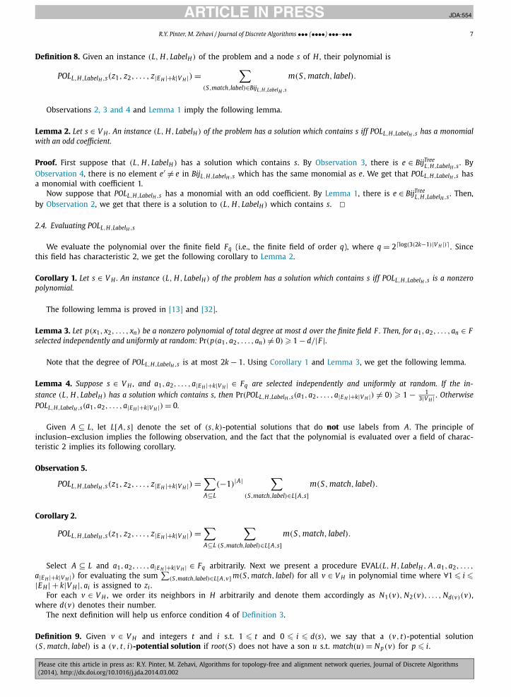
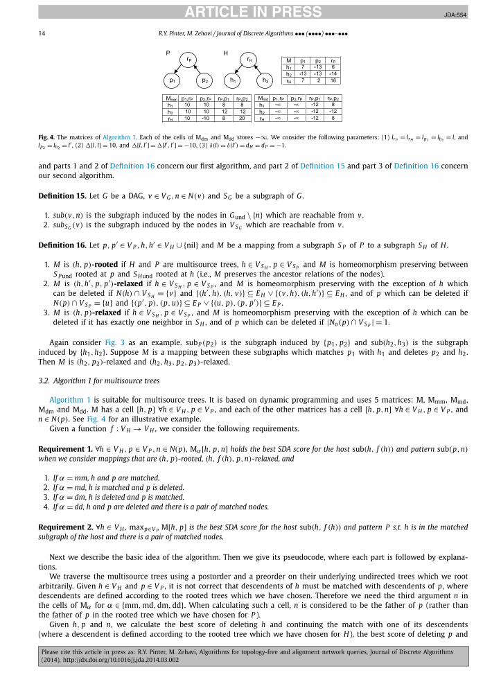
Fig. 4. The matrices of Algorithm 1. Each of the cells of Mdm and Mdd stores −∞. We consider the following parameters: (1) lrP = lrH = lp1 = lh1 = l, andlp2 = lh2 = l′ , (2) �[l, l] = 10, and �[l, l′] = �[l′, l′] = −10, (3) δ(l) = δ(l′) = dH = dP = −1.
and parts 1 and 2 of Definition 16 concern our first algorithm, and part 2 of Definition 15 and part 3 of Definition 16 concernour second algorithm.
Definition 15. Let G be a DAG, v ∈ V G ,n ∈ N(v) and SG be a subgraph of G .
1. sub(v,n) is the subgraph induced by the nodes in Gund \ {n} which are reachable from v .2. subSG (v) is the subgraph induced by the nodes in V SG which are reachable from v .
Definition 16. Let p, p′ ∈ V P ,h,h′ ∈ V H ∪ {nil} and M be a mapping from a subgraph S P of P to a subgraph S H of H .
1. M is (h, p)-rooted if H and P are multisource trees, h ∈ V S H , p ∈ V S P and M is homeomorphism preserving betweenS P und rooted at p and S Hund rooted at h (i.e., M preserves the ancestor relations of the nodes).
2. M is (h,h′, p, p′)-relaxed if h ∈ V S H , p ∈ V S P , and M is homeomorphism preserving with the exception of h whichcan be deleted if N(h) ∩ V S H = {v} and {(h′,h), (h, v)} ⊆ E H ∨ {(v,h), (h,h′)} ⊆ E H , and of p which can be deleted ifN(p) ∩ V S P = {u} and {(p′, p), (p, u)} ⊆ E P ∨ {(u, p), (p, p′)} ⊆ E P .
3. M is (h, p)-relaxed if h ∈ V S H , p ∈ V S P , and M is homeomorphism preserving with the exception of h which can bedeleted if it has exactly one neighbor in S H , and of p which can be deleted if |No(p) ∩ V S P | = 1.
Again consider Fig. 3 as an example. subP (p2) is the subgraph induced by {p1, p2} and sub(h2,h3) is the subgraphinduced by {h1,h2}. Suppose M is a mapping between these subgraphs which matches p1 with h1 and deletes p2 and h2.Then M is (h2, p2)-relaxed and (h2,h3, p2, p3)-relaxed.
3.2. Algorithm 1 for multisource trees
Algorithm 1 is suitable for multisource trees. It is based on dynamic programming and uses 5 matrices: M, Mmm, Mmd,Mdm and Mdd. M has a cell [h, p] ∀h ∈ V H , p ∈ V P , and each of the other matrices has a cell [h, p,n] ∀h ∈ V H , p ∈ V P , andn ∈ N(p). See Fig. 4 for an illustrative example.
Given a function f : V H → V H , we consider the following requirements.
Requirement 1. ∀h ∈ V H , p ∈ V P ,n ∈ N(p), Mα[h, p,n] holds the best SDA score for the host sub(h, f (h)) and pattern sub(p,n)
when we consider mappings that are (h, p)-rooted, (h, f (h), p,n)-relaxed, and
1. If α = mm, h and p are matched.2. If α = md, h is matched and p is deleted.3. If α = dm, h is deleted and p is matched.4. If α = dd, h and p are deleted and there is a pair of matched nodes.
Requirement 2. ∀h ∈ V H , maxp∈V P M[h, p] is the best SDA score for the host sub(h, f (h)) and pattern P s.t. h is in the matchedsubgraph of the host and there is a pair of matched nodes.
Next we describe the basic idea of the algorithm. Then we give its pseudocode, where each part is followed by explana-tions.
We traverse the multisource trees using a postorder and a preorder on their underlying undirected trees which we rootarbitrarily. Given h ∈ V H and p ∈ V P , it is not correct that descendents of h must be matched with descendents of p, wheredescendents are defined according to the rooted trees which we have chosen. Therefore we need the third argument n inthe cells of Mα for α ∈ {mm,md,dm,dd}. When calculating such a cell, n is considered to be the father of p (rather thanthe father of p in the rooted tree which we have chosen for P ).
Given h, p and n, we calculate the best score of deleting h and continuing the match with one of its descendents(where a descendent is defined according to the rooted tree which we have chosen for H), the best score of deleting p and

JID:JDA AID:554 /FLA [m3G; v 1.130; Prn:27/03/2014; 8:21] P.15 (1-25)
R.Y. Pinter, M. Zehavi / Journal of Discrete Algorithms ••• (••••) •••–••• 15
continuing the match with one of its descendents (where a descendent is defined as each of its neighbors excluding n), andthe best score of matching h with p and continuing the match with their descendents. When h and p are matched, we usea maximum weight matching calculation in order to find the best option to match between their descendents.
Algorithm 1.
1. ∀p ∈ V P , n ∈ N(p), calculate δ(p,n) = ∑p′∈V sub(p,n)
δ(lp′ ).
2. ∀G ∈ {H, P }, choose rG ∈ V G . Denote by GrGund the tree Gund rooted at rG , and denote by f (v) the father of v in GrG
und(where f (rG) = nil).
3. ∀h ∈ V H in postorder on HrHund:
(a) ∀p ∈ V P in postorder on P rPund, PostTraverseCalc(h, p).
(b) ∀p ∈ V P in preorder on P rPund, PreTraverseCalc(h, p).
4. Return max{∑p∈V Pδ(lp) + dP ,maxh∈V H ,p∈V P M[h, p]}.
In Step 1 we calculate the cost of deleting sub(p,n) for each p ∈ V P and n ∈ N(p). In Step 3 we traverse H and P inan order that guarantees us that in a calculation of a cell, the cells on which it depends have been already calculated. InStep 4 we return the maximum between the score of deleting all P and the best SDA score for H and P s.t. there is a pairof matched nodes.
PostTraverseCalc(h, p):
1. Denote X = Ni(p), X ′ = {x′: x ∈ X} and Y = Ni(h) \ { f (h)}.2. Construct a bipartite graph Gi with bipartition (X, Y ∪ X ′).
∀x ∈ X , connect x and x′ with an edge whose weight is δ(x, p) + dP , and ∀x ∈ X , y ∈ Y , connect x and y with an edgewhose weight is maxα∈{mm,md,dm,dd} Mα[y, x, p].
3. Calculate W i the maximum weight of a matching in Gi .4. Similarly construct Go and calculate Wo .5. M[h, p] ⇐ �[lh, lp] + W i + Wo .
In Steps 2–4 we construct two bipartite graphs whose maximum weight matchings correspond to the best matchingsbetween the ingoing and outgoing neighbors of h and p. In Step 5 we store the sum of these weights and the score ofmatching h with p in M[h, p].
6. If f (h) = nil, define Rh = ∅. Else if ( f (h),h) ∈ E H , define Rh = No(h). Else define Rh = Ni(h). Similarly define R p .7. ∀n ∈ Ni(p):
(a) Calculate W ni the maximum weight of a matching in Gi \ {n,n′}.
(b) Mmm[h, p,n] ⇐ �[lh, lp] + W ni + Wo .
(c) Mdm[h, p,n] ⇐ δ(lh) + maxh′∈Rh max{Mdm[h′, p,n],Mmm[h′, p,n] + dH }.(d) Mdd[h, p,n] ⇐ δ(lh) + maxh′∈Rh max{Mdd[h′, p,n],Mmd[h′, p,n] + dH }.
8. Similarly calculate Mmm, Mdm and Mdd for h, p and each n ∈ No(p).
In Step 7(a) we update Gi so that its matching will not include n. In Step 7(b) we store the updated sum in Mmm[h, p,n].In Step 7(c) we calculate the sum of the score of deleting h and matching sub(h′,h) with sub(p,n) for the best choice of h′from Rh . We consider only the matrices Mdm and Mmm since we need to match p, and we consider only neighbors of h inRh since we are restricted to (h, f (h), p,n)-relaxed matchings. If h′ is matched, we pay dH for the deletion of h (we start anew component deletion). Step 7(d) is similar.
9. If f (p) �= nil: Mmd[h, p, f (p)] ⇐ δ(p, f (p)) + maxp′∈R p (max{Mmd[h, p′, p],Mmm[h, p′, p] + dP } − δ(p′, p)).
Step 9 is similar to Step 7(c) with the exception that we pay δ(p, f (p)) − δ(p′, p) since we delete all the nodes whichare in sub(p,n) and not in sub(p′, p) (the nodes in P must be either matched or deleted).
PreTraverseCalc(h, p):
1. mdo = maxp′∈No(p)(max{Mmd[h, p′, p],Mmm[h, p′, p]+dP }− δ(p′, p)). ∀n ∈ Ni(p)\ { f (p)}: Mmd[h, p,n] ⇐ δ(p,n)+mdo .2. Similarly calculate Mmd for h, p and each n ∈ No(p) \ { f (p)}.3. ∀p′ ∈ Ni(p):
ip′,d = maxhi∈Ni(h)\{ f (h)} max{Mmd[hi, p′, p],Mdd[hi, p′, p] − dH },ip′,m = maxhi∈Ni(h)\{ f (h)} max{Mmm[hi, p′, p],Mdm[hi, p′, p] − dH },op′,d = maxho∈No(h)\{ f (h)} max{Mmd[ho, p, p′],Mdd[ho, p, p′] − dH },op′,m = maxho∈No(h)\{ f (h)} max{Mmm[ho, p, p′],Mdm[ho, p, p′] − dH }.
JID:JDA AID:554 /FLA [m3G; v 1.130; Prn:27/03/2014; 8:21] P.16 (1-25)
16 R.Y. Pinter, M. Zehavi / Journal of Discrete Algorithms ••• (••••) •••–•••
4. t = maxp′∈Ni(p) max{ip′,d + op′,d − dP , ip′,d + op′,m, ip′,m + op′,d, ip′,m + op′,m}.5. M[h, p] ⇐ max{M[h, p],dH + δ(lh) + t}.
Steps 1 and 2 are similar to Step 9 of PostTraverseCalc. In Steps 3–5 we update M[h, p] if we can get a better score bydeleting h. The deletion of h requires the matching of sub(hi,h) with sub(p′, p) and of sub(ho,h) with sub(p, p′) for somep′ ∈ Ni(p), hi ∈ Ni(h) \ { f (h)} and ho ∈ No(h) \ { f (h)}. t saves the score of the best choice of such p′ , hi and ho .
The following theorem states the correctness and running time of Algorithm 1. We prove it in Sections 3.4 and 3.5. Notethat the algorithm returns the score of a solution. However, we can track its calculations in order to obtain the solutionitself without increasing its time and space complexities.
Theorem 2. Algorithm 1 solves the SDA problem for multisource trees, and it runs in time O (|V P ||V H |(|V P | + log |V H |)). Moreover,it performs in time O (|V P ||V H |( |V P |
log |V P | + log |V H |)) when the number of labels is bounded.
3.3. Algorithm 2 for treelike DAGs
Algorithm 2 is suitable for treelike DAGs s.t. P has one source. The requirement that P has one source is made forthe sake of clarity of presentation. In case P has s > 1 sources v1, v2, . . . , vs , we run a slightly modified version of thisalgorithm s times where in the ith time we use P without nodes that are not reachable from vi . Note that since P has onesource, we get that ∀p ∈ V P , p′ ∈ No(p): frb(p′) ⊆ frb(p) ∪ dsr(p).
The algorithm is based on dynamic programming and uses 4 matrices: Mmm, Mmd, Mdm and Mdd. Each matrix has acell [h, p, S, f , g] ∀h ∈ V H , p ∈ V P , S ⊆ frb(h), 1–1 f : frb(p)+p → S+h , and g : frb(p)+p → 2V H s.t. [∀p′ ∈ frb(p)+p, g(p′) ⊆frb( f (p′)) \ (frb(h) \ S)]. See Fig. 3 for an illustrative example.
We consider the following requirement.
Requirement 3. For each cell [h, p, S, f , g], Mα[h, p, S, f , g] holds the best SDA score for the host subH\(frb(h)\S)(h) and pat-
tern subP (p) when we consider (h, p)-relaxed mappings s.t. [∀p′ ∈ frb(p)+p, p′ is matched with f (p′) ∧ subP (p′) is matched withsubH\(frb( f (p′))\g(p′))( f (p′))], and
1. If α = mm, h and p are matched.2. If α = md, h is matched and p is deleted.3. If α = dm, h is deleted and p is matched.4. If α = dd, h and p are deleted and there is a pair of matched nodes.
Next we describe the basic idea of the algorithm. Then we give its pseudocode, where each part is followed by explana-tions.
We traverse the treelike DAGs in a reverse topological order. Given h ∈ V H and p ∈ V P , we need to know the set S ofnodes from frb(h) which we are allowed to use for matching nodes that can be reached from p, and thus we iterate overeach such set. Moreover, ∀p′ ∈ frb(p)+p we need to know which was the node h′ ∈ frb(h)+h with whom it was previouslymatched, and which nodes from frb(h′) were allowed to be used in order to match nodes which can be reached from p′(see the explanation of Definition 11 in Section 3.1 for intuition why we need this information). Thus we need f and g inthe matrices cells.
Given h, p and the information mentioned above, we calculate the best score of deleting h and continuing the match withone of its outgoing neighbors, the best score of deleting p and continuing the match with one of its outgoing neighbors,and the best score of matching h with p and continuing the match with their outgoing neighbors. When h and p arematched, we use a maximum weight matching calculation in order to find the best option to match between their outgoingneighbors.
Algorithm 2.
1. ∀p ∈ V P , calculate δ(p) = ∑p′∈V subP (p)
δ(lp′ ).
2. ∀v ∈ V H ∪ V P , calculate frb(v) and dsr(v).3. Initialize all the cells of Mmm, Mmd, Mdm and Mdd to −∞.4. ∀h ∈ V H in reverse topological order:
∀p ∈ V P in reverse topological order:For k = 0 . . . |frb(h)|, iterate over each S ⊆ frb(h) of size k:
For each cell [h, p, S, f , g]: Calc(h, p, S, f , g).5. Return
∑p∈V P
δ(lp)+dP + max{0,maxh∈V H ,p∈V P s.t. frb(p)+p=∅(Mmm[h, p, frb(h),∅,∅]− δ(p)−d(p))} where d(p) = dP ifp is the source of P and 0 otherwise.

JID:JDA AID:554 /FLA [m3G; v 1.130; Prn:27/03/2014; 8:21] P.17 (1-25)
R.Y. Pinter, M. Zehavi / Journal of Discrete Algorithms ••• (••••) •••–••• 17
In Step 1 we calculate the cost of deleting subP (p) for each p ∈ V P . In Step 4 we iterate over the cells in an order whichguarantees that in a calculation of a cell, the cells on which it depends have been already calculated. In Step 5 we returnthe maximum between the score of deleting all P and the best SDA score for H and P s.t. there is a pair of matched nodes.We consider only nodes in P whose frb sets are empty and which are not crossroads since Definition 14 restricts us tolimited subgraphs.
Calc(h, p, S, f , g):
1. Denote I = frb(h) \ S .2. If p is not a crossroad:
(a) R p = {p′ ∈ No(p): �v ∈ dsr(p) which is reachable from p′ and �v ∈ frb(p) which is not reachable from p′}.(b) Mmd[h, p, S, f , g] ⇐ δ(p) + maxp′∈R p (max{Mmd[h, p′, S, f , g],Mmm[h, p′, S, f , g] + dP } − δ(p′)).(c) Mdd[h, p, S, f , g] ⇐ δ(p) + maxp′∈R p (max{Mdd[h, p′, S, f , g],Mdm[h, p′, S, f , g] + dP } − δ(p′)).
If p is not a crossroad, we delete it (we cannot delete a crossroad since Definition 14 restricts us to limited subgraphs).In Step 2(b) we calculate the sum of the score of deleting the nodes in subP (p) which are not in subP (p′) and matchingsubH\I (h) with subP (p′) for the best option to choose p′ ∈ R p . Since P has one source, the calculation is legal. We consideronly the matrices Mmm and Mmd since we need to match h, and we consider only neighbors of p in R p since Definition 14restricts us to limited subgraphs. If p′ is matched, we pay dP for the deletion of p (we start a new component deletion).Step 2(c) is similar.
3. Rh = {h′ ∈ No(h) \ I: ∀p′ ∈ frb(p)+p there is a path from h′ to f (p′)}.4. Mdm[h, p, S, f , g] ⇐ δ(lh) + maxh′∈Rh max{Mdm[h′, p, frb(h′) \ I, f , g],Mmm[h′, p, frb(h′) \ I, f , g] + dH }.
Step 4 is similar to Step 2(b), with the exception that we pay only for the deletion of h (the nodes in H can be neithermatched nor deleted). Moreover, the definition of Rh is not symmetric to R p . Here we consider this definition since weneed to choose an outgoing neighbor of h which we are allowed to use (i.e., it is not in I) and from which the nodes thatwe must match in order to be consistent with f are reachable.
The rest of the procedure concerns the calculation of Mmm[h, p, S, f , g].
5. If p is a crossroad:(a) If f (p) �= h, return.(b) Else if g(p) �= S , Mmm[h, p, S, f , g] ⇐ Mmm[h, p, g(p), f , g] and return.
If p is a crossroad and f (p) �= h, we cannot match h with p and thus we return. If p is a crossroad, f (p) = h andg(p) �= S , we have already performed the required calculation for Mmm[h, p, g(p), f , g], and thus we just copy it.
6. ∀v ∈ dsr(p) initialize rep(v) = |{p′ ∈ No(p): v is reachable from p′}|.7. ∀v ∈ dsr(p) in topological order:
(a) fix(v) = −(rep(v) − 1).(b) ∀v ′ ∈ dsr(p) which is reachable from v: add fix(v) to rep(v ′).
In Steps 6 and 7 we calculate fix(v) for each v ∈ dsr(p). These calculations are used in the last part of the algorithm tocorrect the problem that when we match the outgoing neighbors of p, we may consider the scores of matching or deletingnodes in dsr(p) more than once. For example, consider the calculation of Mmm[h3, p3,∅,∅,∅] as in Fig. 3. When matchingNo(p3) with No(h3), we consider the matching of p1 once for each node in No(p3) from whom it is reachable (i.e., once forp1 and once for p2).
8. ∀Del ⊆ dsr(p)\ frb(p) for which {v ∈ (frb(p)∪ (dsr(p)\ Del)): ∃p′ ∈ No(p), u ∈ Del s.t. v and u are reachable from p′} =∅:(a) Denote X = {n ∈ No(p): �v ∈ Del which is reachable from n}, X = No(p) \ X , X ′ = {x′: x ∈ X} and Y = No(h) \ I .(b) Define C = ( X ∪ Del, {{v, u}: u ∈ Del ∩ frb(v)}). Calculate the number nC of connected components in C and D =
nC dP + ∑p′∈ X δ(p′).
We iterate over all the legal options to delete nodes from dsr(p) \ frb(p). Since Definition 12 restricts us to limitedsubgraphs, the deletion of a node v ∈ dsr(p) \ frb(p) determines that all the internal nodes on the paths from p to v aredeleted. Moreover, if a node v is not deleted, we can neither delete nodes from its frb set nor delete nodes of degree greaterthan 2 that have v in their frb or dsr sets. Thus a legal set Del of deleted nodes satisfies {v ∈ (frb(p)∪ (dsr(p) \ Del)): ∃p′ ∈No(p), u ∈ Del s.t. v and u are reachable from p′} = ∅.
In Step 8(b) we calculate D , which is the score of deleting the nodes that were determined as deleted because of Del.
8. (c) ∀ 1–1 f ′ : frb(p)+p ∪ (dsr(p) \ Del) → S+h ∪ (dsr(h) \ I) s.t. [ f ′|frb(p)+p ≡ f ], and

JID:JDA AID:554 /FLA [m3G; v 1.130; Prn:27/03/2014; 8:21] P.18 (1-25)
18 R.Y. Pinter, M. Zehavi / Journal of Discrete Algorithms ••• (••••) •••–•••
∀g′ : frb(p)+p ∪ (dsr(p) \ Del) → 2V H s.t. [g′|frb(p)+p ≡ g ∧ ∀p′, g(p′) ⊆ frb( f ′(p′)) \ I]:i. If ∃p1, p2 s.t. p1 �= p2, there is a path from p1 to p2 and [ f ′(p2) /∈ g′(p1) ∨ g′(p2) ∩ (frb( f ′(p1)) \ g′(p1)) �= ∅],
continue.ii. If ∃p1, p2 s.t. there is no path from p1 to p2 or from p2 to p1 and ∃v ∈ (g′(p1) ∪ { f ′(p1)}) ∩ (g′(p2) ∪ { f ′(p2)})
for which [�u ∈ frb(p1) ∩ frb(p2) s.t. v ∈ g′(u) ∪ { f ′(u)}], continue.
We iterate over all the legal options to choose f ′ and g′ , which are extensions of f and g respectively. f determines themapping of the crossroads in dsr(p)∪ frb(p) which were not determined as deleted, and g′ determines the mapping of theircorresponding subgraphs (i.e., for p′ ∈ dsr(p) ∪ frb(p): if p′ ∈ Del then subP (p′) is deleted, and otherwise [p′ is matchedwith f ′(p′) ∧ subP (p′) is matched with subH\(frb( f ′(p′))\g′(p′))( f ′(p′))])). In particular, Step 8(c)ii is correct since P has onesource.
8. (c) iii. Denote Dsr = {h′ ∈ dsr(h) \ I: �p′ s.t. h′ ∈ g′(p′) ∪ { f ′(p′)}}.iv. ∀d : X → 2Dsr s.t. [∪p′d(p′) = Dsr ∧ ∀p1, p2 ∈ X d(p1) ∩ d(p2) = ∅]:
We iterate over all the options to choose which ‘unused’ nodes in dsr(h) \ I (i.e., nodes in Dsr) can be mapped whenmatching subP (p′) for each p′ ∈ No(p) that was not determined as deleted.
8. (c) iv. A. Construct a bipartite graph G with bipartition (X, Y ∪ X ′). ∀x ∈ X , connect x and x′ with an edge whoseweight is [δ(x) + dP if frb(x)+x = ∅, and −∞ otherwise].∀x ∈ X , y ∈ Y :• Denote Sxy = { f ′(v): v ∈ frb(x)+x} ∪ {v ∈ frb(y)+y: [v ∈ d(x) ∪ S \ dsr(h)] ∨ [∃u ∈ frb(x)+x s.t. v ∈
g′(u)] ∨ [v /∈ frb(h) ∪ dsr(h)]}.• If { }+y ⊆ Sxy ⊆ frb(y)+y , connect x and y with an edge whose weight is maxα∈{mm,md,dm,dd} Mα[y, x,
Sxy \ {y}, f ′|frb(x)+x , g′|frb(x)+x ].• Else connect them with an edge whose weight is −∞.
B. Calculate W the maximum weight of a matching in G .
We calculate the best score of matching the outgoing neighbors of p with the outgoing neighbors of h, which is denotedby W . It is easy to verify that the calculation is correct since Definition 12 restricts us to limited subgraphs and P has onesource. For example, x can be deleted iff it is not a crossroad and its frb set is empty. Therefore we connect x and x′ withan edge whose weight is δ(x) + dP (i.e., the cost of deleting subP (x)) if frb(x)+x = ∅, and −∞ otherwise.
8. (c) iii. C. ∀v ∈ dsr(p): val(v) is δ(v) if v ∈ Del, and Mmm[ f ′(v), v, g′(v), f ′|frb(v)+v , g′|frb(v)+v ] otherwise.D. Denote FIX = ∑
v∈dsr(p) fix(v)val(v).E. If Mmm[h, p, S, f , g] < �[lh, lp] + D + W + FIX: Mmm[h, p, S, f , g] ⇐ �[lh, lp] + D + W + FIX.
We sum the score of matching p with h with the scores D and W . By adding FIX to �[lh, lp]+ D + W , the score of eachmatched pair or deleted node is considered exactly once.
The following theorem states the correctness and running time of Algorithm 2. We prove it in Sections 3.4 and 3.5. Notethat the algorithm returns the score of a solution. However, we can track its calculations in order to obtain the solutionitself without increasing its time and space complexities.
Theorem 3. Algorithm 2 solves the SDA problem for treelike DAGs s.t. P has one source, and it runs in time O (|E P ||V P |max{dsr(H)−1,0} ×|E H |(|V P | + log |V H |) + |V H ||E H |). Moreover, it performs in time O (|V P |( |V P |
log |V P | )max{dsr(H)−1,0}|E H | · (
|V P |log |V P | + log |V H |) +
|V H ||E H |) when P is a directed tree and the number of labels is bounded.
3.4. Correctness
The correctness of Algorithm 1 is based on the following Lemmas 10 and 11.
Lemma 10. Algorithm 1 satisfies Requirement 1.
Proof. First of all, note that each cell depends only on previously computed cells. Thus we can assume that cells which donot depend on other cells are calculated first, and the computation order of all the other cells is as in the algorithm. Weprove the lemma by using induction on this order.
The induction basis includes the following calculations ∀h ∈ V H , p ∈ V P :
• If N(p) = {n}, then Mmm[h, p,n] = �[lh, lp], which is correct since we only need to match h with p.• If Rh = ∅, then ∀n ∈ N(p), α ∈ {dm,dd}, Mα[h, p,n] = −∞, which is correct since in this case h cannot be deleted.

JID:JDA AID:554 /FLA [m3G; v 1.130; Prn:27/03/2014; 8:21] P.19 (1-25)
R.Y. Pinter, M. Zehavi / Journal of Discrete Algorithms ••• (••••) •••–••• 19
• If No(p) = ∅, then ∀n ∈ Ni(p) Mmd[h, p,n] = −∞, which is correct since in this case p cannot be deleted.• If Ni(p) = ∅, then ∀n ∈ No(p) Mmd[h, p,n] = −∞, which is correct since in this case p cannot be deleted.
Now we prove that each calculation which does not belong to the basis of the induction is correct assuming the cells onwhich it depends are correct:
1. For n ∈ Ni(p), Mmm[h, p,n] = �[lh, lp] + W ni + Wo .
We consider mappings which are (h, p)-rooted, (h, f (h), p,n)-relaxed and match h with p. Thus ∀p′ ∈ Ni(p) \ {n},sub(p′, p) is either deleted or matched with a different subgraph sub(h′,h) where h′ ∈ Ni(h) \ { f (h)} using a match-ing which is (h′, p′)-rooted and (h′,h, p′, p)-relaxed. Moreover, ∀p′ ∈ No(p) we have the symmetric claim. Thus thecorrectness of the calculation follows from the induction hypothesis and our maximum weight matching calculation.For n ∈ No(p), the proof of the calculation of Mmm[h, p,n] is symmetric.
2. Mdm[h, p,n] = δ(lh) + maxh′∈Rh max{Mdm[h′, p,n],Mmm[h′, p,n] + dH }.We pay δ(lh) for the deletion of h. We consider mappings which are (h, p)-rooted, (h, f (h), p,n)-relaxed, delete h andmatch p, and thus sub(p,n) must be matched with sub(h′,h) for some h′ ∈ Rh using a mapping which is (h′, p)-rooted,(h′,h, p,n)-relaxed and matches p. Moreover, if h′ is matched, we pay the additional cost dH for the deletion of h. Thecorrectness of the calculation follows from these arguments and the correctness of the induction hypothesis.
3. The proof of the calculation of Mdd[h, p,n] is similar to 2.4. For n ∈ Ni(p),
Mmd[h, p,n] = δ(p,n) + maxp′∈No(p)
(max
{Mmd
[h, p′, p
],Mmm
[h, p′, p
] + dP} − δ
(p′, p
)).
Since we consider mappings which are (h, p)-rooted, (h, f (h), p,n)-relaxed, delete p and match h, sub(h, f (h)) mustbe matched with sub(p′, p) for some p′ ∈ No(p) using a mapping which is (h, p′)-rooted, (h, f (h), p′, p)-relaxed andmatches h. We pay δ(p,n) − δ(p′, p) for the deletion of the nodes in sub(p,n) which are not in sub(p′, p). Moreover, ifp′ is matched, we pay the additional cost dP for the deletion of p. The correctness of the calculation follows from thesearguments and the correctness of the induction hypothesis.For n ∈ No(p), the proof of the calculation of Mmd[h, p,n] is symmetric. �
Lemma 11. Algorithm 1 satisfies Requirement 2.
Proof. Let h be a node in H and p be a node in P . When calculating M[h, p], the cells of the other matrices on whichit depends were already calculated. Thus according to Lemma 10, Step 5 of PostTraverseCalc(h, p) and Steps 3–5 ofPreTraverseCalc(h, p), M[h, p] holds the maximum of the following scores:
• The best SDA score for the host sub(h, f (h)) and pattern P when we consider homeomorphism preserving (h, p)-rootedmappings which match h with p.
• The best SDA score for the host sub(h, f (h)) and pattern P when we consider homeomorphism preserving mappingswhich consist of– A mapping which only deletes h.– A (hi, p′)-rooted and (hi,h, p′, p)-relaxed mapping between sub(hi,h) and sub(p′, p).– A (ho, p)-rooted and (ho,h, p, p′)-relaxed mapping between sub(ho,h) and sub(p, p′).for some p′ ∈ Ni(p),hi ∈ Ni(h) \ { f (h)} and ho ∈ No(h) \ { f (h)}. We define this score as −∞ in case no such mappingexists.
Note that the best SDA score for the host sub(h, f (h)) and pattern P is equal to the maximum of these scores for somep ∈ V P and is equal or bigger from these scores for all the other nodes of P . Thus we derive the lemma. �
The correctness of Algorithm 2 is based on the following Lemma 12.
Lemma 12. Algorithm 2 satisfies Requirement 3.
Proof. First of all, note that each cell depends only on previously computed cells. Thus we can assume that cells which donot depend on other cells are calculated first, and the computation order of all the other cells is as in the algorithm. Weprove the lemma by using induction on this order.
The induction basis includes the following calculations for each [h, p, S, f , g]:
• If p is a crossroad or R p = ∅, Mmd[h, p, S, f , g] = Mdd[h, p, S, f , g] = −∞, which is correct since in this case there areno matchings as the lemma requires which delete p (we consider only limited subgraphs of P ).
• If Rh = ∅, Mdm[h, p, S, f , g] = −∞, which is correct since in this case there are no matchings as the lemma requireswhich delete h.
JID:JDA AID:554 /FLA [m3G; v 1.130; Prn:27/03/2014; 8:21] P.20 (1-25)
20 R.Y. Pinter, M. Zehavi / Journal of Discrete Algorithms ••• (••••) •••–•••
• If p is a crossroad and f (p) �= h, or we reach Step 8 of Calc(h, p, S, f , g) though no bipartite graph is constructed, thenMmm[h, p, S, f , g] remains −∞ as it is initialized, since in this case there are no matchings as the lemma requireswhich match p with h. Else if a bipartite graph is constructed in Step 8 of Calc(h, p, S, f , g), and No(p) = ∅ or No(h) \I = ∅, Mmm[h, p, S, f , g] = �[lh, lp] + D + FIX. This is the score of matching p with h and deleting all the other nodesin subP (p), which is the only legal option in this case.
Now we prove that each calculation which does not belong to the basis of the induction is correct assuming the cells onwhich it depends are correct:
1. Mmd[h, p, S, f , g] ⇐ δ(p) + maxp′∈R p (max{Mmd[h, p′, S, f , g],Mmm[h, p′, S, f , g] + dP } − δ(p′)).In order to fulfill the requirements of the lemma, subH\I (h) must be matched with subP (p′) for some p′ ∈ R p using amapping which is (h, p′)-relaxed, matches h, and [∀v ∈ frb(p′)+p′
, v is matched with f (v) ∧ subP (v) is matched withsubH\(frb( f (v))\g(v))
( f (v))] (note that ∀p′ ∈ R p , frb(p′)+p′ = frb(p)+p ). We pay δ(p)−δ(p′) for the deletion of the nodesin subP (p) which are not in subP (p′). Moreover, if p′ is matched, we pay the additional cost dP for the deletion of p.The correctness of the calculation follows from these arguments and the correctness of the induction hypothesis.
2. The proof of the calculation of Mdd[h, p, S, f , g] is similar to 1.3. Mdm[h, p, S, f , g] ⇐ δ(lh) + maxh′∈Rh max{Mdm[h′, p, frb(h′) \ I, f , g],Mmm[h′, p, frb(h′) \ I, f , g] + dH }.
We pay δ(lh) for the deletion of h. In order to fulfill the requirements of the lemma, subP (p) must be matched withsubH\I (h′) for some h′ ∈ Rh using a mapping which is (h′, p)-relaxed, matches p, and [∀v ∈ frb(p)+p, v is matchedwith f (v) ∧ subP (v) is matched with subH\(frb( f (v))\g(v))
( f (v))]. The correctness of the calculation follows from thesearguments and the correctness of the induction hypothesis.
4. If p is a crossroad, f (p) = h and g(p) �= S , the correctness of the calculation Mmm[h, p, S, f , g] ⇐ Mmm[h, p, g(p), f , g]follows immediately from the requirements of the lemma.Otherwise when calculating Mmm[h, p, S, f , g] we perform an exhaustive search for the best of all the legal optionsto choose Del, f ′, g′ and d, which determine the deletions or matchings of all the nodes in dsr(p) ∪ frb(p) and theircorresponding subgraphs (i.e., for p′ ∈ dsr(p)∪ frb(p): if p′ ∈ Del then subP (p′) is deleted, and otherwise [p′ is matchedwith f ′(p′) ∧ subP (p′) is matched with subH\(frb( f ′(p′))\g′(p′))( f ′(p′))]) and which nodes from dsr(h) can be used whenmatching subP (p′) for each p′ ∈ No(p). For each such option we calculate the best matching of the subgraphs corre-sponding to nodes in No(p) which may not be deleted with deletions or with the subgraphs corresponding to nodes inNo(h) \ I , whose correctness follows from the maximum weight matching calculation the algorithm performs and theinduction hypothesis. We add this result to the score of matching p with h and deleting the subgraphs correspondingto nodes in No(p) which were determined as deleted by Del. By adding FIX to �[lh, lp] + D + W , the score of eachmatched pair or deleted node is considered exactly once, and thus the calculation is correct. �
3.5. Running time analysis
Given p ∈ V P and p′ ∈ N(p), denote:
1. iso(p′, p) is {n ∈ N(p): there is an isomorphism between sub(n, p) and sub(p′, p), which is also an isomorphismbetween their underlying undirected trees rooted at n and p′, respectively} if P is a multisource tree, and {p′}
otherwise.2. As(p) = {iso(n, p): n ∈ N(p)}, and A(p) = |As(p)|.
Lemma 13. For a multisource tree P whose number of labels is bounded, we have that ∀p ∈ V P : A(p) = O (|V P |
log |V P | ).
Proof. Denote by f (n) the number of distinct labeled multisource trees in a forest of n nodes which have a unique node.Shamir et al. [34] prove that the number of distinct labeled rooted trees in a forest of n nodes is O ( n
log n ). In their proof,they use the rooted tree topology only when claiming that the number of distinct unlabeled rooted trees on i nodes is atmost ci for some constant c. We have 2i−1 options to direct the edges of each of them (some of them may result in thesame tree). We treat their roots as their unique nodes. Thus the number of unlabeled multisource trees on i nodes whichhave a unique node is at most ci for some constant c, and we can use the same proof to show that f (n) = O ( n
log n ). Thelemma follows by observing that ∀p ∈ V P : A(p) � f (|V P |). �
Given a bipartite graph G = (X, Y ∪ X ′, E) that is constructed in Algorithm 1 or 2 according to the nodes h ∈ V H , p ∈V P and the weight function w : E → R , denote by X∗ the partition of X into sets s.t. x1, x2 ∈ X are in the same set iffw(x1, x′
1) = w(x2, x′2) ∧ ∀y ∈ Y : w(x1, y) = w(x2, y). Note that |X | � |N(p)|, |Y | � |N(h)| and A(p) � |N(p)|. Moreover,
|X∗| = O (A(p)) since if x1 and x2 belong to the same set in As(p) and if d(x1) = d(x2) (in case G is constructed inAlgorithm 2), then x1 and x2 belong to the same set in X∗ .
Lemma 14. A maximum weight matching in G can be computed in time O (|X |[|X∗||Y | + (|X∗| + |Y |) log(|X∗| + |Y |)]).
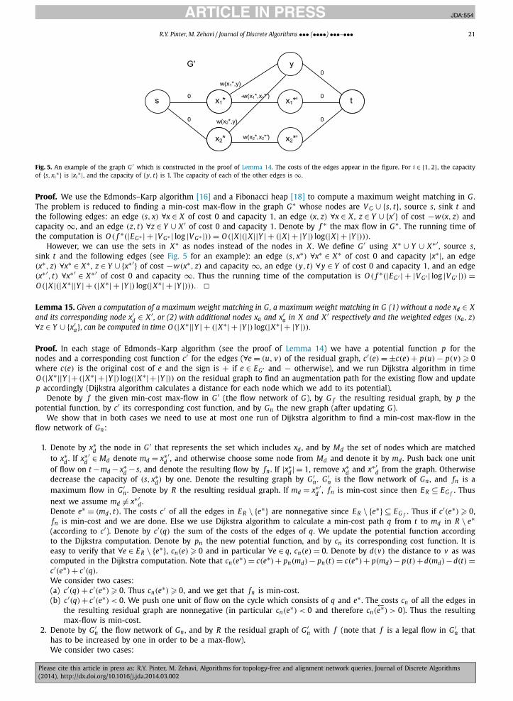
JID:JDA AID:554 /FLA [m3G; v 1.130; Prn:27/03/2014; 8:21] P.21 (1-25)
R.Y. Pinter, M. Zehavi / Journal of Discrete Algorithms ••• (••••) •••–••• 21
Fig. 5. An example of the graph G ′ which is constructed in the proof of Lemma 14. The costs of the edges appear in the figure. For i ∈ {1,2}, the capacityof {s, xi
∗} is |xi∗|, and the capacity of {y, t} is 1. The capacity of each of the other edges is ∞.
Proof. We use the Edmonds–Karp algorithm [16] and a Fibonacci heap [18] to compute a maximum weight matching in G .The problem is reduced to finding a min-cost max-flow in the graph G∗ whose nodes are V G ∪ {s, t}, source s, sink t andthe following edges: an edge (s, x) ∀x ∈ X of cost 0 and capacity 1, an edge (x, z) ∀x ∈ X , z ∈ Y ∪ {x′} of cost −w(x, z) andcapacity ∞, and an edge (z, t) ∀z ∈ Y ∪ X ′ of cost 0 and capacity 1. Denote by f ∗ the max flow in G∗ . The running time ofthe computation is O ( f ∗(|EG∗ | + |V G∗ | log |V G∗ |)) = O (|X |(|X ||Y | + (|X | + |Y |) log(|X | + |Y |))).
However, we can use the sets in X∗ as nodes instead of the nodes in X . We define G ′ using X∗ ∪ Y ∪ X∗′ , source s,sink t and the following edges (see Fig. 5 for an example): an edge (s, x∗) ∀x∗ ∈ X∗ of cost 0 and capacity |x∗|, an edge(x∗, z) ∀x∗ ∈ X∗ , z ∈ Y ∪ {x∗′} of cost −w(x∗, z) and capacity ∞, an edge (y, t) ∀y ∈ Y of cost 0 and capacity 1, and an edge(x∗′, t) ∀x∗′ ∈ X∗′ of cost 0 and capacity ∞. Thus the running time of the computation is O ( f ∗(|EG ′ | + |V G ′ | log |V G ′ |)) =O (|X |(|X∗||Y | + (|X∗| + |Y |) log(|X∗| + |Y |))). �Lemma 15. Given a computation of a maximum weight matching in G, a maximum weight matching in G (1) without a node xd ∈ Xand its corresponding node x′
d ∈ X ′ , or (2) with additional nodes xa and x′a in X and X ′ respectively and the weighted edges (xa, z)
∀z ∈ Y ∪ {x′a}, can be computed in time O (|X∗||Y | + (|X∗| + |Y |) log(|X∗| + |Y |)).
Proof. In each stage of Edmonds–Karp algorithm (see the proof of Lemma 14) we have a potential function p for thenodes and a corresponding cost function c′ for the edges (∀e = (u, v) of the residual graph, c′(e) = ±c(e) + p(u) − p(v) � 0where c(e) is the original cost of e and the sign is + if e ∈ EG ′ and − otherwise), and we run Dijkstra algorithm in timeO (|X∗||Y |+ (|X∗|+ |Y |) log(|X∗|+ |Y |)) on the residual graph to find an augmentation path for the existing flow and updatep accordingly (Dijkstra algorithm calculates a distance for each node which we add to its potential).
Denote by f the given min-cost max-flow in G ′ (the flow network of G), by G f the resulting residual graph, by p thepotential function, by c′ its corresponding cost function, and by Gn the new graph (after updating G).
We show that in both cases we need to use at most one run of Dijkstra algorithm to find a min-cost max-flow in theflow network of Gn:
1. Denote by x∗d the node in G ′ that represents the set which includes xd , and by Md the set of nodes which are matched
to x∗d . If x∗
d′ ∈ Md denote md = x∗
d′ , and otherwise choose some node from Md and denote it by md . Push back one unit
of flow on t −md − x∗d − s, and denote the resulting flow by fn . If |x∗
d| = 1, remove x∗d and x∗′
d from the graph. Otherwisedecrease the capacity of (s, x∗
d) by one. Denote the resulting graph by G ′n . G ′
n is the flow network of Gn , and fn is amaximum flow in G ′
n . Denote by R the resulting residual graph. If md = x∗d′ , fn is min-cost since then E R ⊆ EG f . Thus
next we assume md �= x∗′d .
Denote e∗ = (md, t). The costs c′ of all the edges in E R \ {e∗} are nonnegative since E R \ {e∗} ⊆ EG f . Thus if c′(e∗) � 0,fn is min-cost and we are done. Else we use Dijkstra algorithm to calculate a min-cost path q from t to md in R \ e∗(according to c′). Denote by c′(q) the sum of the costs of the edges of q. We update the potential function accordingto the Dijkstra computation. Denote by pn the new potential function, and by cn its corresponding cost function. It iseasy to verify that ∀e ∈ E R \ {e∗}, cn(e) � 0 and in particular ∀e ∈ q, cn(e) = 0. Denote by d(v) the distance to v as wascomputed in the Dijkstra computation. Note that cn(e∗) = c(e∗)+ pn(md)− pn(t) = c(e∗)+ p(md)− p(t)+d(md)−d(t) =c′(e∗) + c′(q).We consider two cases:(a) c′(q) + c′(e∗) � 0. Thus cn(e∗)� 0, and we get that fn is min-cost.(b) c′(q)+ c′(e∗) < 0. We push one unit of flow on the cycle which consists of q and e∗ . The costs cn of all the edges in
the resulting residual graph are nonnegative (in particular cn(e∗) < 0 and therefore cn(←−e∗) > 0). Thus the resulting
max-flow is min-cost.2. Denote by G ′
n the flow network of Gn , and by R the residual graph of G ′n with f (note that f is a legal flow in G ′
n thathas to be increased by one in order to be a max-flow).We consider two cases:
JID:JDA AID:554 /FLA [m3G; v 1.130; Prn:27/03/2014; 8:21] P.22 (1-25)
22 R.Y. Pinter, M. Zehavi / Journal of Discrete Algorithms ••• (••••) •••–•••
(a) xa belongs to a set x∗a which is already a node in G ′ . Then G ′
n is G ′ where the capacity of (s, x∗a) is increased by one.
Since E R \ EG f = {(s, x∗a)}, the costs c′ of all the other edges in R are nonnegative.
We use Dijkstra algorithm to compute a min-cost path q from x∗a to t in R without (s, x∗
a), push one unit of flow onthe path which consists of (s, x∗
a) and q, and update the potential function accordingly. If the cost corresponding tothe new potential of (x∗
a , s) is negative, we add it to the potential of s. It is easy to verify that the costs correspondingto the new potential of all the edges in the resulting residual graph are nonnegative, and thus we have a min-costmax-flow.
(b) xa does not belong to a set x∗a which is already a node in G ′ . We define p(x∗
a) = p(s), p(x∗′a) = p(t) and extend
c′ accordingly. The only edges in R which may have negative costs c′ are (x∗a , z) for z ∈ Y ∪ {x∗′
a} since c′(s, x∗a) =
c′(x∗′a, t) = c′(t, x∗′
a) = 0 and all the other edges exist in G f .We subtract m = minz∈Y ∪{x∗′
a}c′(x∗a , z) from the original cost c of each edge (x∗
a , z) s.t. z ∈ Y ∪{x∗′a}. Since we subtract
m from the costs of all the max flows, a max-flow is min-cost when using the new costs iff it is min-cost whenusing the original costs. The costs c′ of all the edges in R are now nonnegative. We use one run of Dijksra algorithmto find an augmentation path for the existing flow f and update p to pn accordingly. Then the costs of all the edgesin the resulting residual graph (according to the cost function corresponding to pn) are nonnegative, and we have amin-cost max-flow. �
Now we can prove the running time of Algorithm 1.
Lemma 16. The running time of Algorithm 1 is O (|V P ||V H |(|V P | + log |V H |)), and O (|V P ||V H |( |V P |log |V P | + log |V H |)) when the
number of labels is bounded.
Proof. The running time of the initialization and all the PostTraverseCalc and PreTraverseCalc calls excluding the maximumweight matching computations is bounded by O (|V P ||V H |).
In PostTraverseCalc, ∀h ∈ V H , p ∈ V P we construct Gi and Go and calculate W i and Wo in time O (|N(p)|[A(p)|N(h)| +(A(p)+|N(h)|) log(A(p)+|N(h)|)]) according to Lemma 14. Then, according to Lemma 15, ∀n ∈ N(p) we calculate W n
i usingGi or W n
o using Go in time O (A(p)|N(h)| + (A(p) + |N(h)|) log(A(p) + |N(h)|)).The total running time is
O
( ∑h∈V H ,p∈V P
(∣∣N(p)∣∣[A(p)
∣∣N(h)∣∣ + (
A(p) + ∣∣N(h)∣∣) log
(A(p) + ∣∣N(h)
∣∣)]) + |V P ||V H |)
= O
(|V H |
∑p∈V P
∣∣N(p)∣∣A(p) + |V H ||V P | log |V H |
)
We get the required running time by using A(p) � |N(p)| and Lemma 13. �We prove two more lemmas and then the running time of Algorithm 2.
Lemma 17. Given a treelike DAG G = (V , E), the time required for computing the dsr and frb sets of all its nodes is bounded byO (|V ||E|).
Proof. Given v, u ∈ V , Q(v, u) denotes a query which returns true if u ∈ dsr(v) and false otherwise. We use the datastructure presented in [38] for directed graphs, which allows us to perform a query Q(v, u) in time O (1) after the insertionof V and E . For general directed graphs, the insertion of E is done in time O (|V |2|E|). We will show that for DAGs it canbe done in time O (|V ||E|).
The structure is initialized by inserting V in time O (|V |2). ∀v ∈ V the structure holds a tree T v . When inserting an edgee, it updates the tree T v of each v s.t. ∃u ∈ V which is reachable from v , but was not reachable from v before the insertionof e. Updating a tree is done in time O (|V |). We compute a reverse topological order v1, . . . , v |V | of V . For i = 1 . . . |V |, weinsert all the outgoing edges of vi . Assume we are inserting the edge (vi, x), and consider a node v j . If j < i, T v j does notneed an update since there is no path from v j to vi because of the reverse topological order. If i < j, T v j does not needan update since there is no path from v j to vi because we have not yet inserted any edge outgoing from v j . If j = i, T v j
might need an update. Thus we insert E in time O (|V ||E|).We compute dsr(v) ∀v ∈ V by iterating over each u ∈ V and performing the query Q(v, u). Afterwards we iterate over
every three different nodes v, u ∈ V and d ∈ dsr(v), and insert d to frb(u) iff d is reachable from u and u is reachablefrom v . Since ∀v ∈ V dsr(v) is bounded, we compute the dsr and frb values of all the nodes in time O (|V |2). Therefore thetotal time is bounded by O (|V ||E|). �Lemma 18. In Calc(h, p, S, f , g) Step 8(c)iv, it is sufficient to iterate over k = O (A(p)|dsr(h)|) functions.
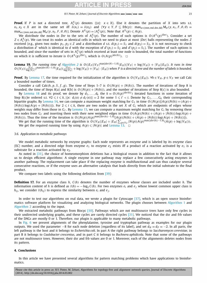
JID:JDA AID:554 /FLA [m3G; v 1.130; Prn:27/03/2014; 8:21] P.23 (1-25)
R.Y. Pinter, M. Zehavi / Journal of Discrete Algorithms ••• (••••) •••–••• 23
Proof. If P is not a directed tree, A Xs (p) denotes {{x}: x ∈ X}. Else it denotes the partition of X into sets s.t.
x1, x2 ∈ X are in the same set iff δ(x1) = δ(x2) and (∀y ∈ Y , F ⊆ frb(y): maxα∈{mm,md,dm,dd} Mα(y, x1, F ,∅,∅) =maxα∈{mm,md,dm,dd} Mα(y, x2, F ,∅,∅)). Denote A X (p) = |A X
s (p)|. Note that A X (p) � A(p).We distribute the nodes in Dsr to the sets of A X
s (p). The number of such options is O (A X (p)|Dsr|). Consider a setZ ∈ A X
s (p). We can treat its nodes as identical cells in which we need to place at most |Dsr| balls representing the nodes Zreceived (e.g., given two nodes p1, p2 ∈ Z and a distribution d s.t. d(p1) = S1 and d(p2) = S2, it is not necessary to checka distribution d′ which is identical to d with the exception of d′(p1) = S2 and d′(p2) = S1). The number of such options isbounded, and since the number of sets in A X
s (p) which received at least one node is bounded, the total number of functionson which it is sufficient to iterate is O (A X (p)|Dsr|), which is O (A(p)|dsr(h)|). �Lemma 19. The running time of Algorithm 2 is O (|E P ||V P |max{dsr(H)−1,0}|E H |(|V P | + log |V H |) + |V H ||E H |). It runs in timeO (|V P |( |V P |
log |V P | )max{dsr(H)−1,0}|E H |( |V P |
log |V P | + log |V H |) + |V H | · |E H |) when P is a directed tree and the number of labels is bounded.
Proof. By Lemma 17, the time required for the initialization of the algorithm is O (|V H ||E H |). ∀h ∈ V H , p ∈ V P we call Calca bounded number of times.
Consider a call Calc(h, p, S, f , g). The time of Steps 1–7 is O (|N(p)| + |N(h)|). The number of iterations of Step 8 isbounded, the time of Steps 8(a) and 8(b) is O (|N(p)| + |N(h)|), and the number of iterations of Step 8(c) is also bounded.
By Lemma 18 and its proof, we denote by d1, . . . ,dk the k = O (A(p)|dsr(h)|) iterated functions in some iteration ofStep 8(c)iv ordered s.t. ∀2 � i � k, |{x: di(x) �= di′ (x)}| = 2 for some 1 � i′ < i. Denote by G1, . . . , Gk their correspondingbipartite graphs. By Lemma 14, we can compute a maximum weight matching for G1 in time O (|N(p)|[A(p)|N(h)|+(A(p)+|N(h)|) log(A(p) + |N(h)|)]). For 2 � i � k, there are two nodes in the set X of Gi which are endpoints of edges whoseweights may differ from those in Gi′ . By Lemma 15, we can compute a maximum weight matching for Gi by removing thesetwo nodes from Gi′ and inserting them with their new weighted edges in time O (A(p)|N(h)| + (A(p) + |N(h)|) log(A(p) +|N(h)|)). Thus the time of the iteration is O (|N(p)|A(p)max{|dsr(h)|−1,0}[A(p)|N(h)| + (A(p) + |N(h)|) log(A(p) + |N(h)|)]).
We get that the running time of the algorithm is O (|V H ||E H | + |E H |∑p∈V P|N(p)|A(p)max{|dsr(h)|−1,0}(A(p) + log |V H |)).
We get the required running time by using A(p) � |N(p)| and Lemma 13. �3.6. Application to metabolic pathways
We model metabolic networks by enzyme graphs: Each node represents an enzyme and is labeled by its enzyme class(EC) number, and a directed edge from enzyme e1 to enzyme e2 exists iff a product of a reaction activated by e1 is asubstrate for a reaction activated by e2.
As noted in [31], the choice of homeomorphism deletions has a biological reason in addition to the fact that it allowsus to design efficient algorithms: A single enzyme in one pathway may replace a few consecutively acting enzymes inanother pathway. The replacement can take place if the replacing enzyme is multifunctional and can thus catalyze severalconsecutive reactions, or if the enzyme uses an alternative catalysis that leads directly from the initial substrate to the finalproduct.
We compare two labels using the following definition from [39]:
Definition 17. For an enzyme class h, C(h) denotes the number of enzymes whose classes are included under h. Theinformation content of h is defined as I(h) = − log2 C(h). For two enzymes ei and e j whose lowest common upper class ishij , we consider I(hij) to express the similarity between ei and e j .
In order to test our algorithms on real data, we wrote a plugin for Cytoscape [37], which is an open source bioinfor-matics software platform for visualizing and analyzing biological networks. The plugin chooses between Algorithm 1 andAlgorithm 2 according to the input.
We extracted metabolic pathways from Biocyc [10]. Pathways which are not multisource trees have only few cycles intheir undirected underlying graphs, and these cycles are rarely directed cycles [31]. We noticed that the dsr and frb valuesof the DAGs are mostly 0 or 1. Therefore, our plugin is applicable to many metabolic pathways.
In Fig. 6 we present alignments of the phenylalanine, tyrosine and tryptophan pathway as examples for our pluginoutputs. We used the parameter −8 for each node deletion (regardless of its label), and set dH = dP = −2. In all parts, theleft pathway is the host and it belongs to Escherichia coli. In part A the right pathway belongs to Saccharomyces cerevisiae, inpart B it belongs to Caulobacter crescentus, and in part C it belongs to Buchnera aphidicola. Note that some of the pathwaysare not multisource trees. However, their dsr and frb values are 0 or 1. Moreover, each of the alignments deletes nodes fromits pattern.
4. Conclusions
In this article we have presented several algorithms for pattern matching problems which have applications to bioinfor-matics.
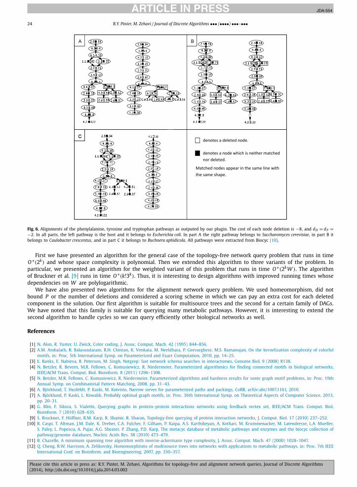
JID:JDA AID:554 /FLA [m3G; v 1.130; Prn:27/03/2014; 8:21] P.24 (1-25)
24 R.Y. Pinter, M. Zehavi / Journal of Discrete Algorithms ••• (••••) •••–•••
Fig. 6. Alignments of the phenylalanine, tyrosine and tryptophan pathways as outputed by our plugin. The cost of each node deletion is −8, and dH = dP =−2. In all parts, the left pathway is the host and it belongs to Escherichia coli. In part A the right pathway belongs to Saccharomyces cerevisiae, in part B itbelongs to Caulobacter crescentus, and in part C it belongs to Buchnera aphidicola. All pathways were extracted from Biocyc [10].
First we have presented an algorithm for the general case of the topology-free network query problem that runs in timeO ∗(2k) and whose space complexity is polynomial. Then we extended this algorithm to three variants of the problem. Inparticular, we presented an algorithm for the weighted variant of this problem that runs in time O ∗(2k W ). The algorithmof Bruckner et al. [9] runs in time O ∗(k!3k). Thus, it is interesting to design algorithms with improved running times whosedependencies on W are polylogarithmic.
We have also presented two algorithms for the alignment network query problem. We used homeomorphism, did notbound P or the number of deletions and considered a scoring scheme in which we can pay an extra cost for each deletedcomponent in the solution. Our first algorithm is suitable for multisource trees and the second for a certain family of DAGs.We have noted that this family is suitable for querying many metabolic pathways. However, it is interesting to extend thesecond algorithm to handle cycles so we can query efficiently other biological networks as well.
References
[1] N. Alon, R. Yuster, U. Zwick, Color coding, J. Assoc. Comput. Mach. 42 (1995) 844–856.[2] A.M. Ambalath, R. Balasundaram, R.H. Chintan, K. Venkata, M. Neeldhara, P. Geevarghese, M.S. Ramanujan, On the kernelization complexity of colorful
motifs, in: Proc. 5th International Symp. on Parameterized and Exact Computation, 2010, pp. 14–25.[3] E. Banks, E. Nabieva, R. Peterson, M. Singh, Netgrep: fast network schema searches in interactomes, Genome Biol. 9 (2008) R138.[4] N. Betzler, R. Bevern, M.R. Fellows, C. Komusiewicz, R. Niedermeier, Parameterized algorithmics for finding connected motifs in biological networks,
IEEE/ACM Trans. Comput. Biol. Bioinform. 8 (2011) 1296–1308.[5] N. Betzler, M.R. Fellows, C. Komusiewicz, R. Niedermeier, Parameterized algorithms and hardness results for some graph motif problems, in: Proc. 19th
Annual Symp. on Combinatorial Pattern Matching, 2008, pp. 31–43.[6] A. Björklund, T. Husfeldt, P. Kaski, M. Koivisto, Narrow sieves for parameterized paths and packings, CoRR, arXiv:abs/1007.1161, 2010.[7] A. Björklund, P. Kaski, L. Kowalik, Probably optimal graph motifs, in: Proc. 36th International Symp. on Theoretical Aspects of Computer Science, 2013,
pp. 20–31.[8] G. Blin, F. Sikora, S. Vialette, Querying graphs in protein–protein interactions networks using feedback vertex set, IEEE/ACM Trans. Comput. Biol.
Bioinform. 7 (2010) 628–635.[9] S. Bruckner, F. Hüffner, R.M. Karp, R. Shamir, R. Sharan, Topology-free querying of protein interaction networks, J. Comput. Biol. 17 (2010) 237–252.
[10] R. Caspi, T. Altman, J.M. Dale, K. Dreher, C.A. Fulcher, F. Gilham, P. Kaipa, A.S. Karthikeyan, A. Kothari, M. Krummenacker, M. Latendresse, L.A. Mueller,S. Paley, L. Popescu, A. Pujar, A.G. Shearer, P. Zhang, P.D. Karp, The metacyc database of metabolic pathways and enzymes and the biocyc collection ofpathway/genome databases, Nucleic Acids Res. 38 (2010) 473–479.
[11] B. Chazelle, A minimum spanning tree algorithm with inverse-ackermann type complexity, J. Assoc. Comput. Mach. 47 (2000) 1028–1047.[12] Q. Cheng, R.W. Harrison, A. Zelikovsky, Homomorphisms of multisource trees into networks with applications to metabolic pathways, in: Proc. 7th IEEE
International Conf. on Bioinform. and Bioengineering, 2007, pp. 350–357.
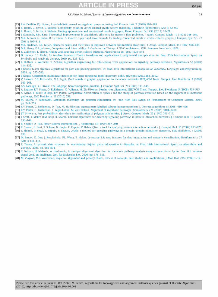
JID:JDA AID:554 /FLA [m3G; v 1.130; Prn:27/03/2014; 8:21] P.25 (1-25)
R.Y. Pinter, M. Zehavi / Journal of Discrete Algorithms ••• (••••) •••–••• 25
[13] R.A. DeMillo, R.J. Lipton, A probabilistic remark on algebraic program testing, Inf. Process. Lett. 7 (1978) 193–195.[14] R. Dondi, G. Fertin, S. Vialette, Complexity issues in vertex-colored graph pattern matching, J. Discrete Algorithms 9 (2011) 82–99.[15] R. Dondi, G. Fertin, S. Vialette, Finding approximate and constrained motifs in graphs, Theor. Comput. Sci. 438 (2013) 10–21.[16] J. Edmonds, R.M. Karp, Theoretical improvements in algorithmic efficiency for network flow problems, J. Assoc. Comput. Mach. 19 (1972) 248–264.[17] M.R. Fellows, G. Fertin, D. Hermelin, S. Vialette, Upper and lower bounds for finding connected motifs in vertex-colored graphs, J. Comput. Syst. Sci. 77
(2011) 799–811.[18] M.L. Fredman, R.E. Tarjan, Fibonacci heaps and their uses in improved network optimization algorithms, J. Assoc. Comput. Mach. 34 (1987) 596–615.[19] M.R. Garey, D.S. Johnson, Computers and Intractability: A Guide to the Theory of NP-Completeness, W.H. Freeman, New York, 1979.[20] S. Guillemot, F. Sikora, Finding and counting vertex-colored subtrees, Algorithmica 65 (2013) 828–844.[21] D. Harvey, D.S. Roche, An in-place truncated Fourier transform and applications to polynomial multiplication, in: Proc. 35th International Symp. on
Symbolic and Algebraic Comput, 2010, pp. 325–329.[22] F. Hüffner, S. Wernicke, T. Zichner, Algorithm engineering for color-coding with applications to signaling pathway detection, Algorithmica 52 (2008)
114–132.[23] I. Koutis, Faster algebraic algorithms for path and packing problems, in: Proc. 35th International Colloquium on Automata, Languages and Programming,
2008, pp. 575–586.[24] I. Koutis, Constrained multilinear detection for faster functional motif discovery, CoRR, arXiv:abs/1206.3483, 2012.[25] V. Lacroix, C.G. Fernandes, M.F. Sagot, Motif search in graphs: application to metabolic networks, IEEE/ACM Trans. Comput. Biol. Bioinform. 3 (2006)
360–368.[26] A.S. LaPaugh, R.L. Rivest, The subgraph homeomorphism problem, J. Comput. Syst. Sci. 20 (1980) 133–149.[27] A. Lozano, R.Y. Pinter, O. Rokhlenko, G. Valiente, M. Ziv-Ukelson, Seeded tree alignment, IEEE/ACM Trans. Comput. Biol. Bioinform. 5 (2008) 503–513.[28] A. Mano, T. Tuller, O. Béjà, R.Y. Pinter, Comparative classification of species and the study of pathway evolution based on the alignment of metabolic
pathways, BMC Bioinform. 11 (2010) S38.[29] M. Mucha, P. Sankowski, Maximum matchings via gaussian elimination, in: Proc. 45th IEEE Symp. on Foundations of Computer Science, 2004,
pp. 248–255.[30] R.Y. Pinter, O. Rokhlenko, D. Tsur, M. Ziv-Ukelson, Approximate labelled subtree homeomorphism, J. Discrete Algorithms 6 (2008) 480–496.[31] R.Y. Pinter, O. Rokhlenko, E. Yeger-Lotem, M. Ziv-Ukelson, Alignment of metabolic pathways, Bioinformatics 21 (2005) 3401–3408.[32] J.T. Schwartz, Fast probabilistic algorithms for verification of polynomial identities, J. Assoc. Comput. Mach. 27 (1980) 701–717.[33] J. Scott, T. Ideker, R.M. Karp, R. Sharan, Efficient algorithms for detecting signaling pathways in protein interaction networks, J. Comput. Biol. 13 (2006)
133–144.[34] R. Shamir, D. Tsur, Faster subtree isomorphism, J. Algorithms 33 (1999) 267–280.[35] R. Sharan, B. Dost, T. Shlomi, N. Gupta, E. Ruppin, V. Bafna, QNet: a tool for querying protein interaction networks, J. Comput. Biol. 15 (2008) 913–925.[36] T. Shlomi, D. Segal, E. Ruppin, R. Sharan, QPath: a method for querying pathways in a protein–protein interaction networks, BMC Bioinform. 7 (2006)
199.[37] M. Smoot, K. Ono, J. Ruscheinski, P.L. Wang, T. Ideker, Cytoscape 2.8: new features for data integration and network visualization, Bioinformatics 27
(2011) 431–432.[38] T. Tholey, A dynamic data structure for maintaining disjoint paths information in digraphs, in: Proc. 14th International Symp. on Algorithms and
Comput., 2003, pp. 565–574.[39] Y. Tohsato, H. Matsuda, A. Hashimoto, A multiple alignment algorithm for metabolic pathway analysis using enzyme hierarchy, in: Proc. 8th Interna-
tional Conf. on Intelligent Syst. for Molecular Biol, 2000, pp. 376–383.[40] M. Vingron, M.S. Waterman, Sequence alignment and penalty choice, review of concepts, case studies and implications, J. Mol. Biol. 235 (1994) 1–12.