Embed Size (px)
Citation preview
Aliasing & Antialiasing
Aaron BloomfieldCS 445: Introduction to Graphics
Fall 2006(Slide set originally by David Luebke)
2
Overview
Introduction Signal Processing Sampling Theorem Prefiltering Supersampling Continuous Antialiasing Catmull's Algorithm The A-Buffer Stochastic Sampling
3
Antialiasing
Aliasing: signal processing term with very specific meaning
Aliasing: computer graphics term for any unwanted visual artifact
Antialiasing: computer graphics term for avoiding unwanted artifacts
We’ll tackle these in order
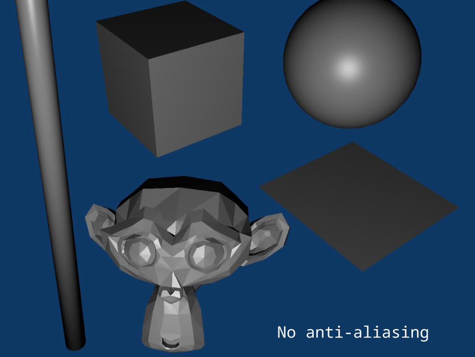
4No anti-aliasing

55 sample anti-aliasing
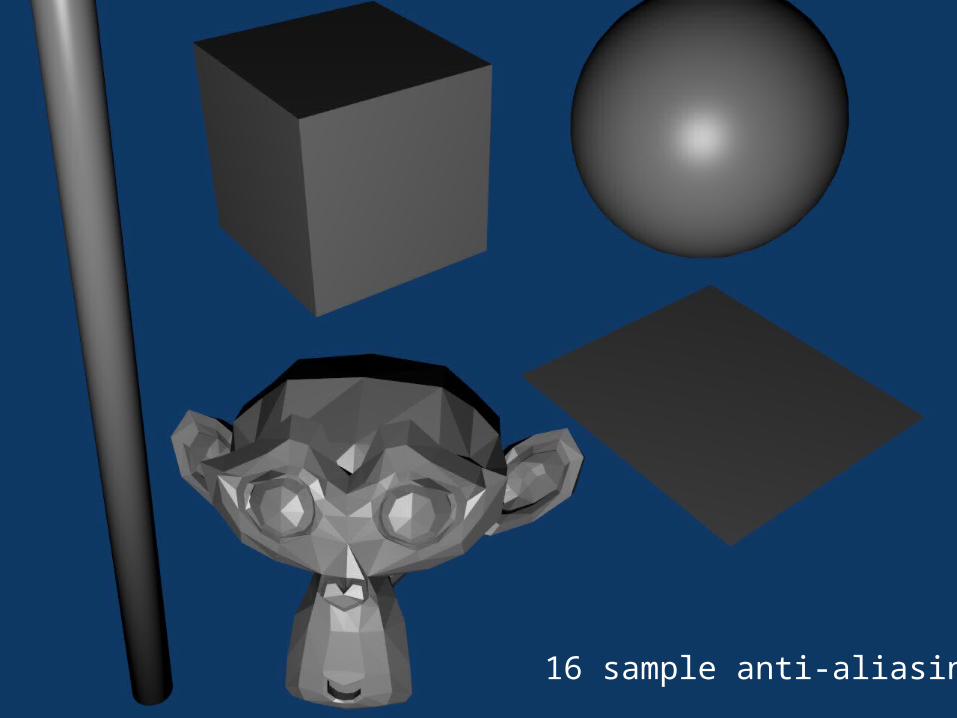
616 sample anti-aliasing
7
Overview
Introduction Signal Processing Sampling Theorem Prefiltering Supersampling Continuous Antialiasing Catmull's Algorithm The A-Buffer Stochastic Sampling
8
Signal Processing
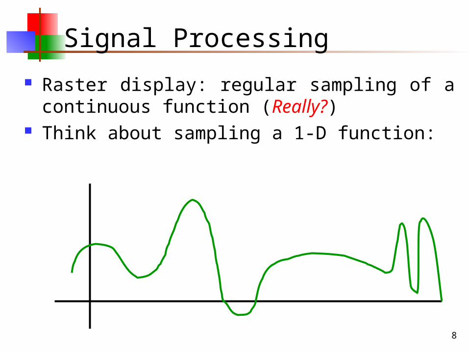
Raster display: regular sampling of a continuous function (Really?)
Think about sampling a 1-D function:
9
Signal Processing
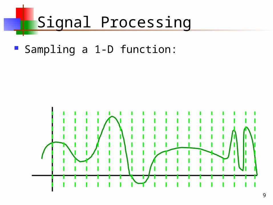
Sampling a 1-D function:
10
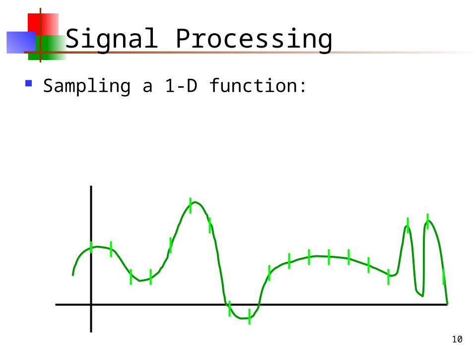
Signal Processing
Sampling a 1-D function:
11
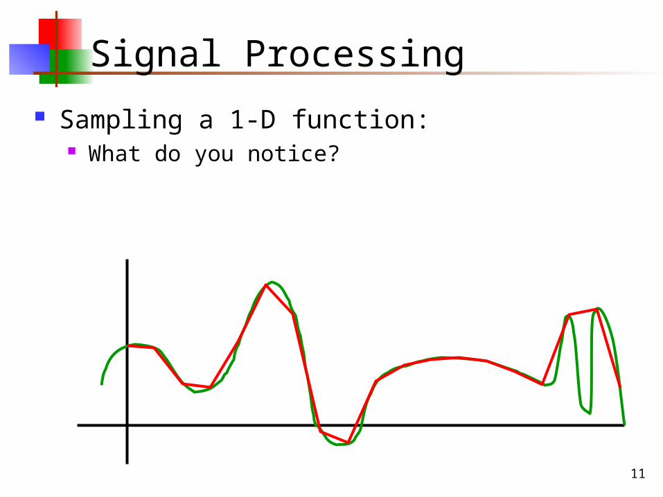
Signal Processing
Sampling a 1-D function: What do you notice?
12
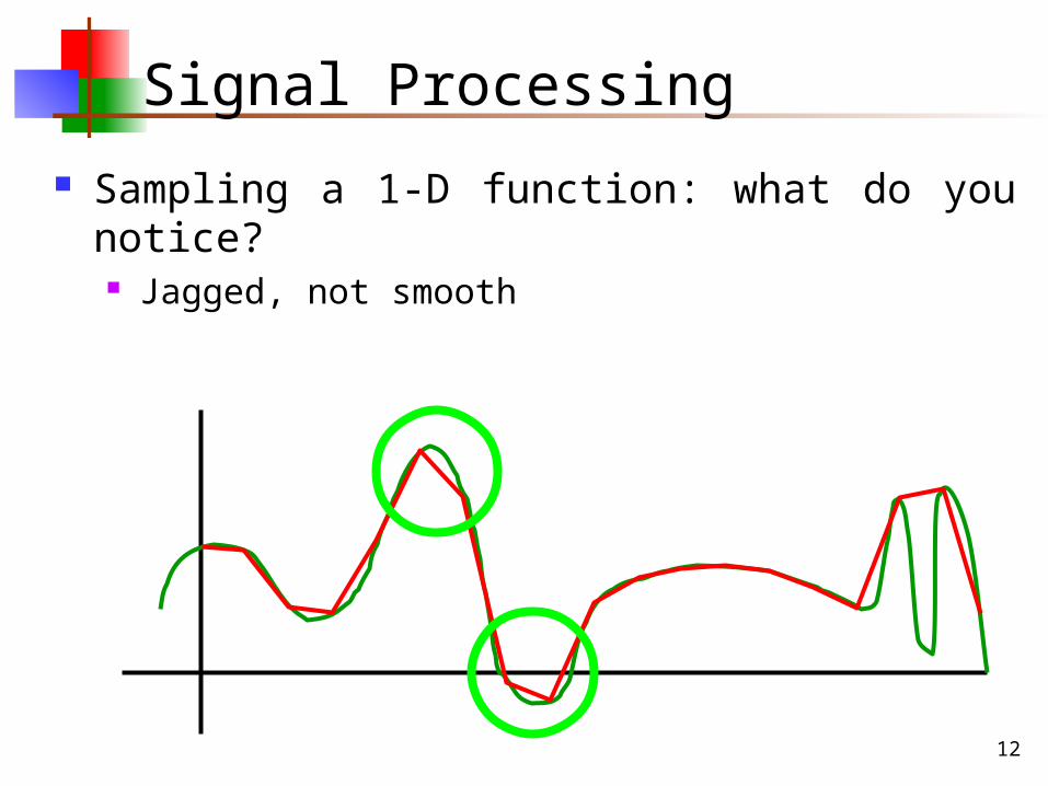
Signal Processing
Sampling a 1-D function: what do you notice? Jagged, not smooth
13
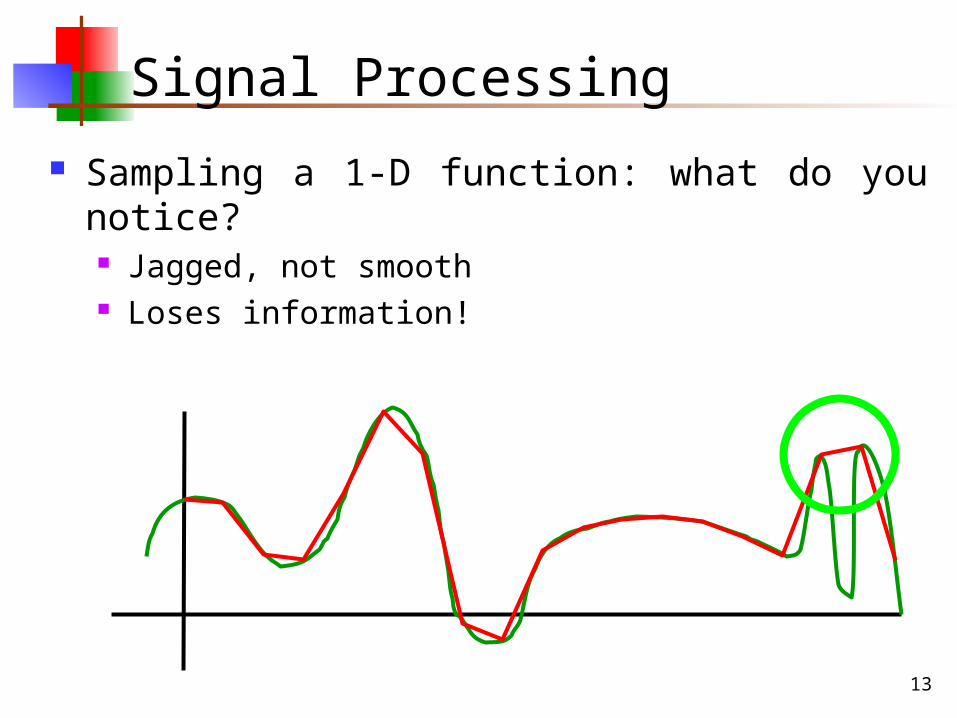
Signal Processing
Sampling a 1-D function: what do you notice? Jagged, not smooth Loses information!
14
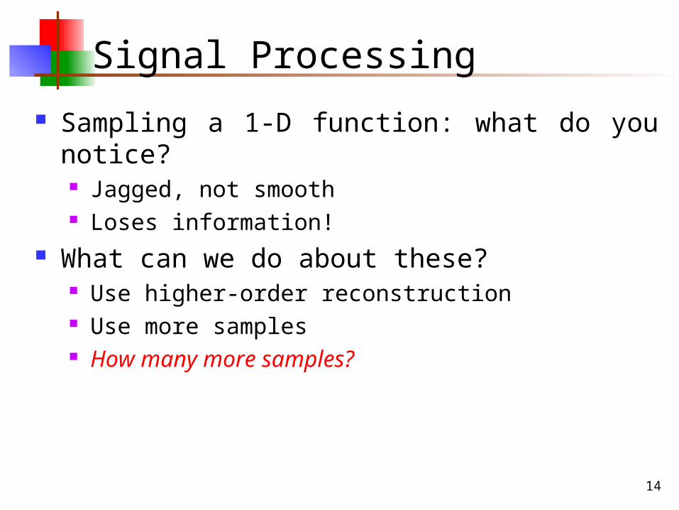
Signal Processing
Sampling a 1-D function: what do you notice? Jagged, not smooth Loses information!
What can we do about these? Use higher-order reconstruction Use more samples How many more samples?
15
Overview
Introduction Signal Processing Sampling Theorem Prefiltering Supersampling Continuous Antialiasing Catmull's Algorithm The A-Buffer Stochastic Sampling
16
The Sampling Theorem
Obviously, the more samples we take the better those samples approximate the original function
The Nyquist sampling theorem:A continuous bandlimited function can be completely represented by a set of equally spaced samples, if the samples occur at more than twice the frequency of the highest frequency component of the function
17
The Sampling Theorem
In other words, to adequately capture a function with maximum frequency F, we need to sample it at frequency N = 2F.
N is called the Nyquist limit.
The Nyquist sampling theorem applied to CDs Most humans can hear to 20 kHz
Some (like me!) to 22 kHz CDs are sampled at 44.1 kHz
Although not twice the “highest frequency component”, it is twice the “highest frequency component” that can be (generally) heard
18
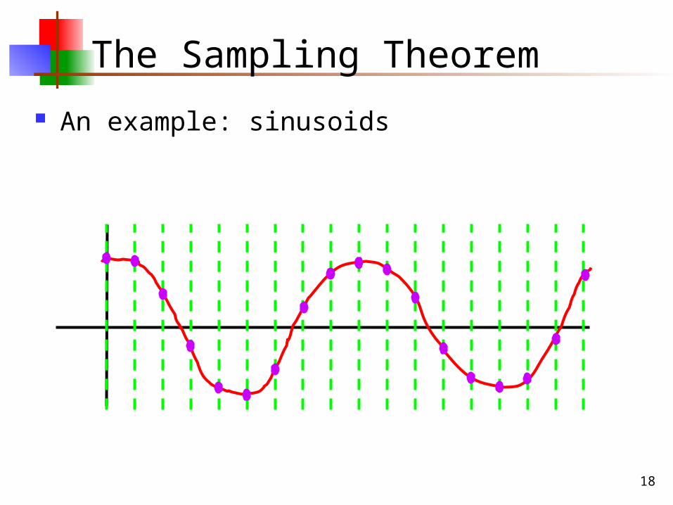
The Sampling Theorem
An example: sinusoids
19
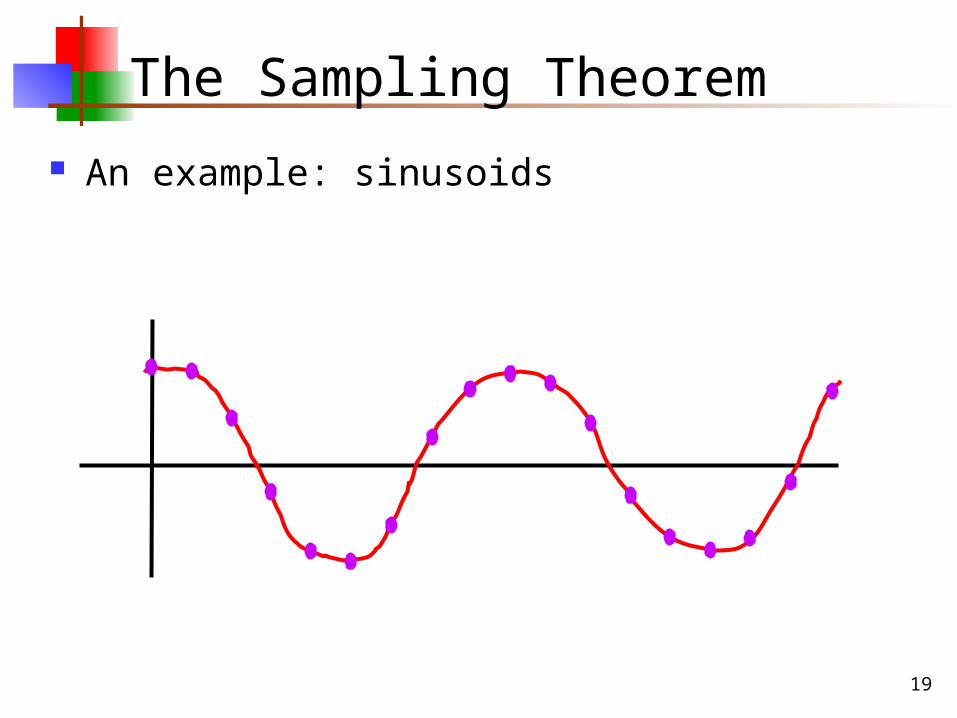
The Sampling Theorem
An example: sinusoids
20
Fourier Theory
All our examples have been sinusoids Does this help with real world signals? Why? Fourier theory lets us decompose any signal into
the sum of (a possibly infinite number of) sine waves
21
Overview
Introduction Signal Processing Sampling Theorem Prefiltering Supersampling Continuous Antialiasing Catmull's Algorithm The A-Buffer Stochastic Sampling
22
Prefiltering
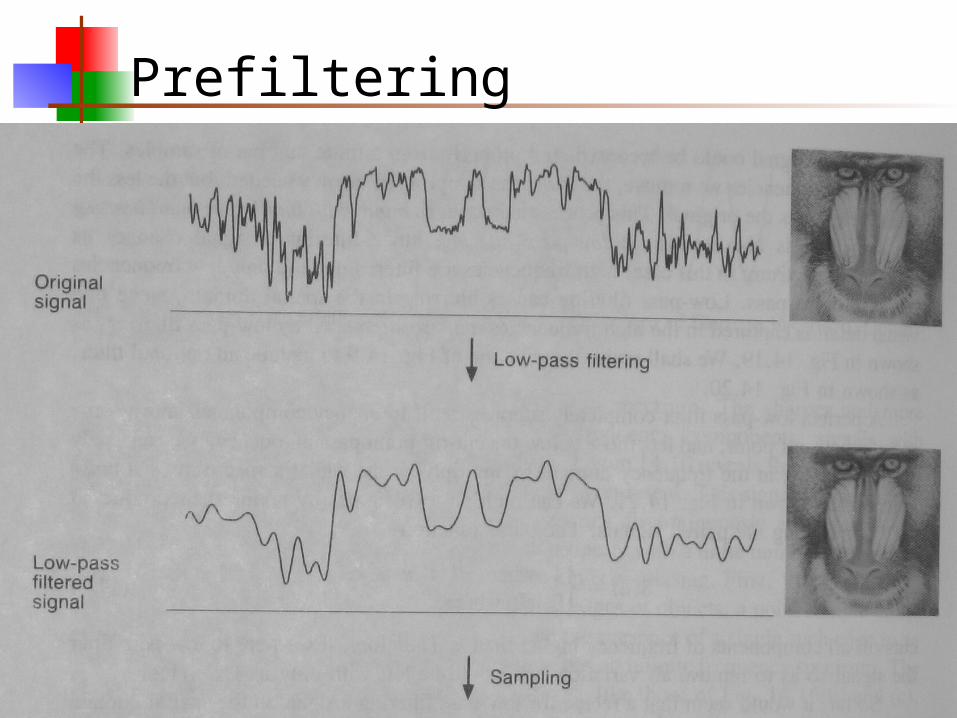
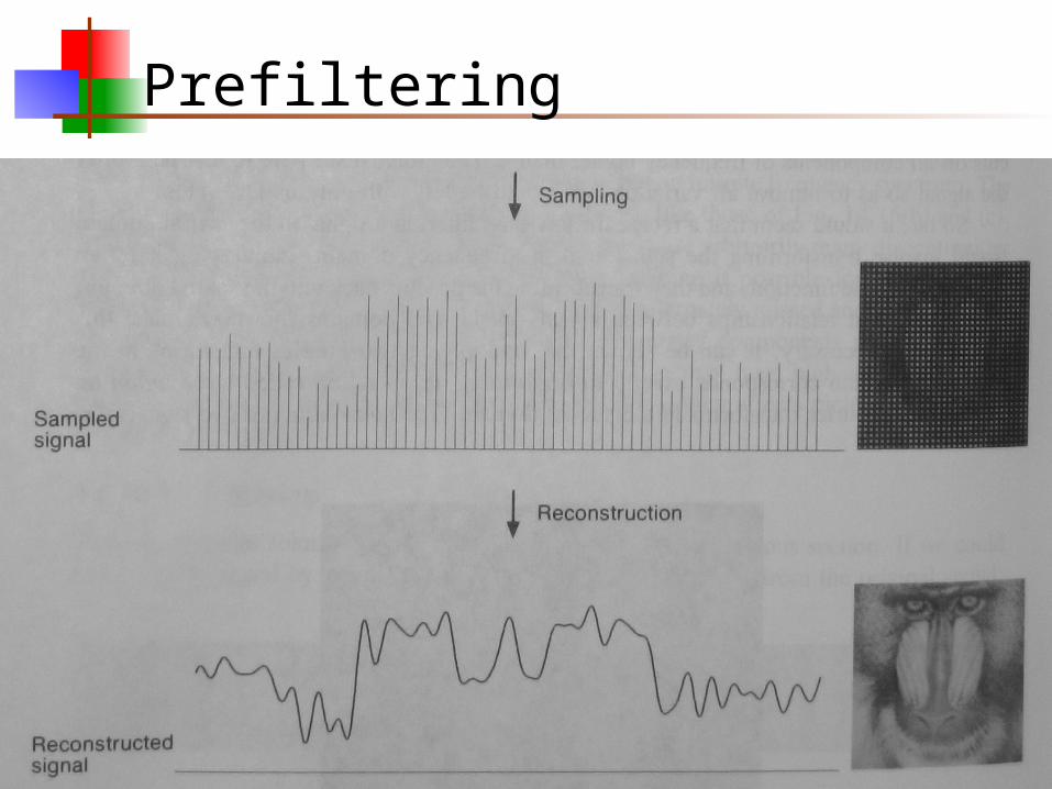
Eliminate high frequencies before sampling (Foley & van Dam p. 630) Convert I(x) to F(u) Apply a low-pass filter
A low-pass filter allows low frequencies through, but attenuates (or reduces) high frequencies
Then sample. Result: no aliasing!
23
Prefiltering
24
Prefiltering
25
Prefiltering
So what’s the problem? Problem: most rendering algorithms generate
sampled function directly e.g., Z-buffer, ray tracing
26
Overview
Introduction Signal Processing Sampling Theorem Prefiltering Supersampling Continuous Antialiasing Catmull's Algorithm The A-Buffer Stochastic Sampling
27
Supersampling
The simplest way to reduce aliasing artifacts is supersampling Increase the resolution of the samples Average the results down
For now, we’ll assume that the samples are evenly spaced In the “Stochastic Sampling” section, we’ll see other
ways of doing it Sometimes called postfiltering
Create virtual image at higher resolution than the final image
Apply a low-pass filter Resample filtered image
28
Supersampling: Limitations
Q: What practical consideration hampers super-sampling?
A: Storage goes up quadratically Q: What theoretical problem does supersampling
suffer? A: Doesn’t eliminate aliasing! Supersampling
simply shifts the Nyquist limit higher
29
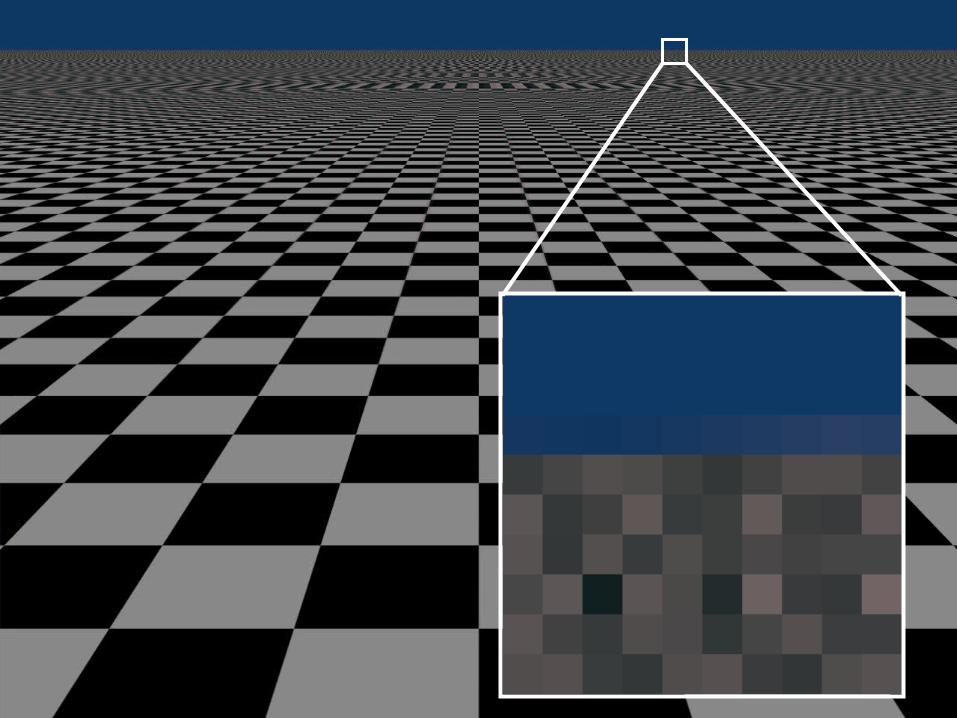
Supersampling: Worst Case
Q: Give a simple scene containing infinite frequencies
A: A checkered ground plane receding into infinity See next slide…
30
31
Supersampling
Despite these limitations, people still use super-sampling (why?)
So how can we best perform it?
32
Supersampling
The process:1. Create virtual image at higher resolution than the final
image
2. Apply a low-pass filter
3. Resample filtered image
33
Supersampling: Step 1
Create virtual image at higher resolution than the final image This is easy
34
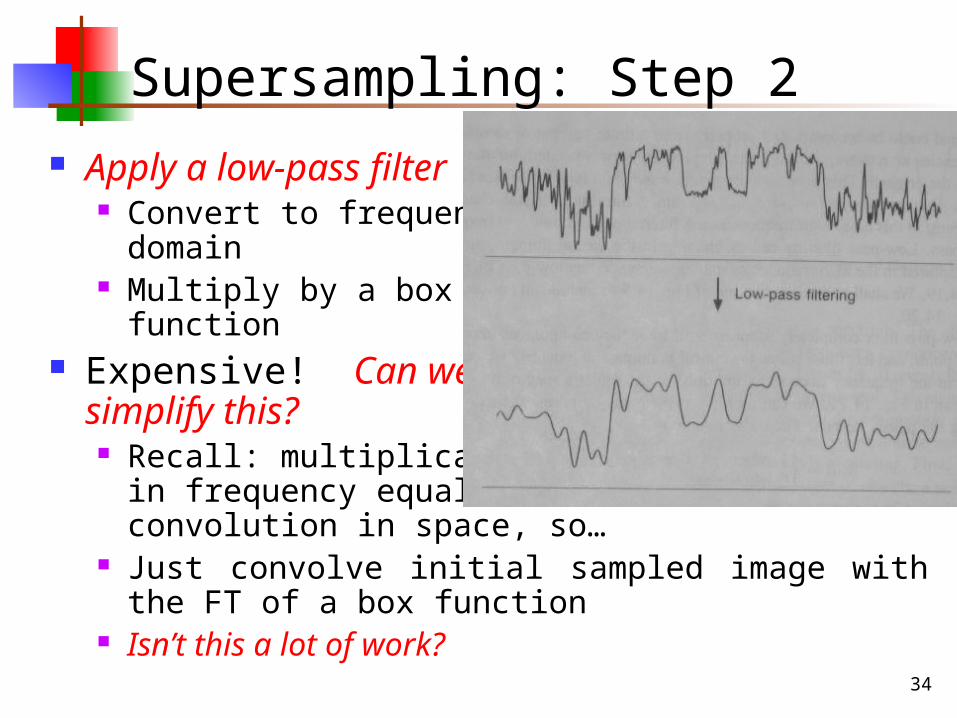
Supersampling: Step 2
Apply a low-pass filter Convert to frequency
domain Multiply by a box
function Expensive! Can we
simplify this? Recall: multiplication
in frequency equals convolution in space, so…
Just convolve initial sampled image with the FT of a box function
Isn’t this a lot of work?
35
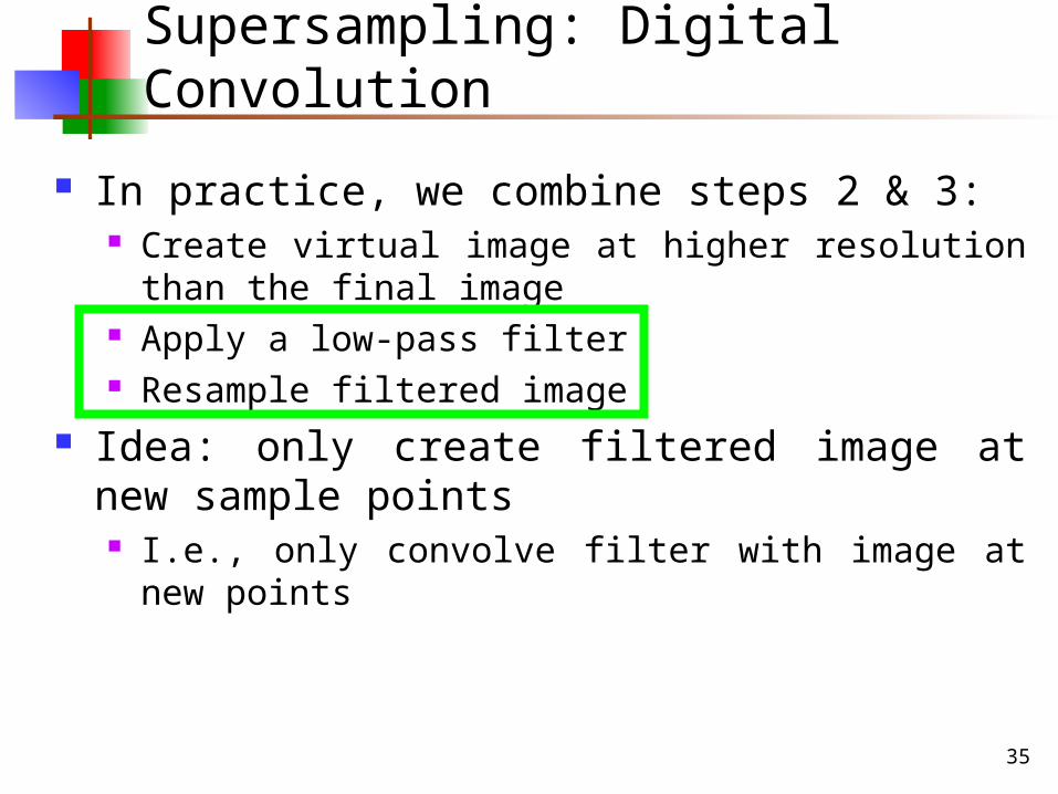
Supersampling: Digital Convolution
In practice, we combine steps 2 & 3: Create virtual image at higher resolution than the final
image Apply a low-pass filter Resample filtered image
Idea: only create filtered image at new sample points I.e., only convolve filter with image at new points
36
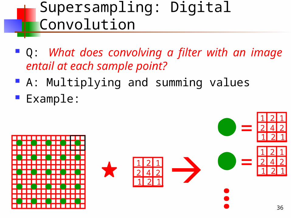
Supersampling: Digital Convolution
Q: What does convolving a filter with an image entail at each sample point?
A: Multiplying and summing values Example:
1 2 12 4 21 2 1
1 2 12 4 21 2 1=1 2 12 4 21 2 1=…
37
Supersampling
Typical supersampling algorithm: Compute multiple samples per pixel Combine sample values for pixel’s value using simple
average Q: What filter does this equate to? A: Box filter -- one of the worst! Q: What’s wrong with box filters?
Passes infinitely high frequencies Attenuates desired frequencies
38
Supersampling
Common filters: Truncated sinc
sinc(x) = sin(x)/x Box Triangle Guassian
39
Supersampling In Practice
Sinc function: ideal but impractical One approximation: sinc2
Another: Gaussian falloff Q: How wide (what res) should filter be? A: As wide as possible (duh) In practice: 3x3, 5x5, at most 7x7
In other words, the filter is larger than the final pixel So we are using the values of neighboring pixels
This creates a better visual effect
40
Supersampling: Summary
Supersampling improves aliasing artifacts by shifting the Nyquist limit
It works by calculating a high-res image and filtering down to final res
“Filtering down” means simultaneous convolution and resampling
This equates to a weighted average Wider filter better results more work
41
Summary So Far
Prefiltering Before sampling the image, use a low-pass filter to
eliminate frequencies above the Nyquist limit This blurs the image… But ensures that no high frequencies will be
misrepresented as low frequencies
42
Summary So Far
Supersampling Sample image at higher resolution than final image, then
“average down” “Average down” means multiply by low-pass function in
frequency domain Which means convolving by that function’s FT in space
domain Which equates to a weighted average of nearby
samples at each pixel
43
Summary So Far
Supersampling cons Doesn’t eliminate aliasing, just shifts the Nyquist limit
higher Can’t fix some scenes (e.g., checkerboard)
Badly inflates storage requirements Supersampling pros
Relatively easy Often works all right in practice Can be added to a standard renderer
44
Overview
Introduction Signal Processing Sampling Theorem Prefiltering Supersampling Continuous Antialiasing Catmull's Algorithm The A-Buffer Stochastic Sampling
45
Antialiasing in the Continuous Domain
Problem with prefiltering: Sampling and image generation inextricably linked in
most renderers Z-buffer algorithm Ray tracing
Why? Still, some approaches try to approximate effect of
convolution in the continuous domain
46
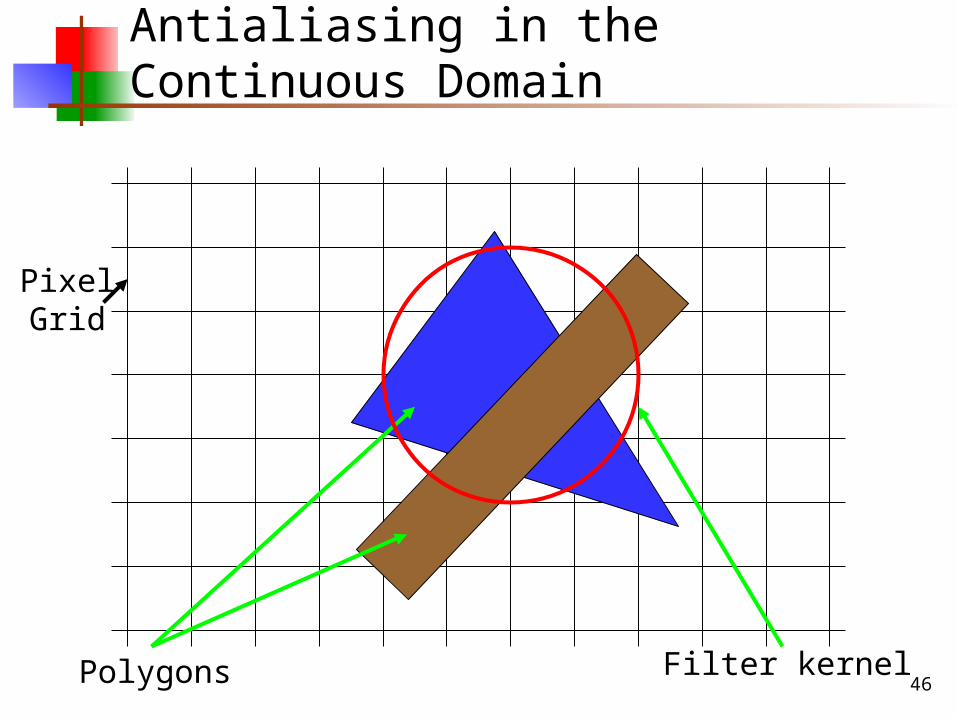
Antialiasing in the Continuous Domain
PixelGrid
Polygons Filter kernel
47
Antialiasing in the Continuous Domain
The good news Exact polygon coverage of the filter kernel can be
evaluated What does this entail?
Clipping Hidden surface determination
48
Antialiasing in the Continuous Domain
The bad news Evaluating coverage is very expensive The intensity variation is too complex to integrate over
the area of the filter Q: Why does intensity make it harder? A: Because polygons might not be flat- shaded Q: How bad a problem is this? A: Intensity varies slowly within a pixel, so shape changes are
more important
49
Overview
Introduction Signal Processing Sampling Theorem Prefiltering Supersampling Continuous Antialiasing Catmull's Algorithm The A-Buffer Stochastic Sampling
50
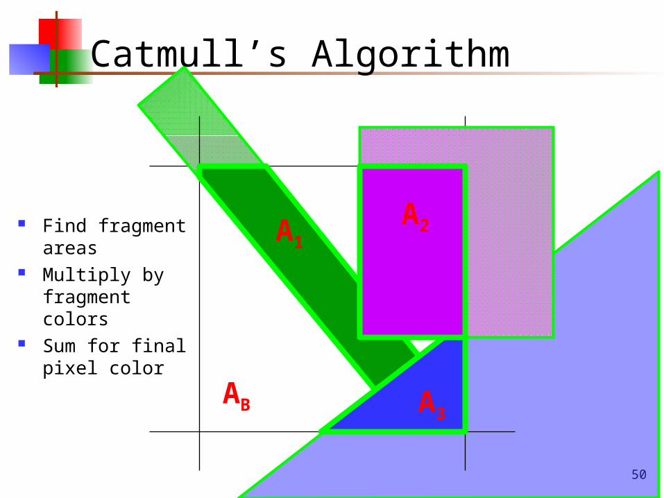
Catmull’s Algorithm
AB
A1A2
A3
Find fragment areas
Multiply by fragment colors
Sum for final pixel color
51
Catmull’s Algorithm
First real attempt to filter in continuous domain Very expensive
Clipping polygons to fragments Sorting polygon fragments by depth (What’s wrong with
this as a hidden surface algorithm?) Equates to box filter (Is that good?)
52
Overview
Introduction Signal Processing Sampling Theorem Prefiltering Supersampling Continuous Antialiasing Catmull's Algorithm The A-Buffer Stochastic Sampling
53
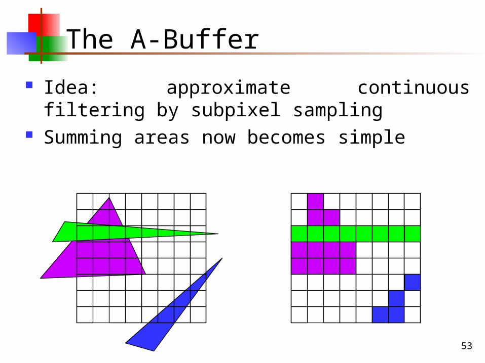
The A-Buffer
Idea: approximate continuous filtering by subpixel sampling
Summing areas now becomes simple
54
The A-Buffer
Advantages: Incorporating into scanline renderer reduces storage
costs dramatically Processing per pixel depends only on number of visible
fragments Can be implemented efficiently using bitwise logical ops
on subpixel masks
55
The A-Buffer
Disadvantages Still basically a supersampling algorithm Not a hardware-friendly algorithm
Lists of potentially visible polygons can grow without limit Work per-pixel non-deterministic
56
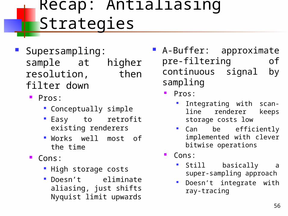
Recap: Antialiasing Strategies
Supersampling: sample at higher resolution, then filter down
Pros: Conceptually simple Easy to retrofit existing
renderers Works well most of the time
Cons: High storage costs Doesn’t eliminate aliasing,
just shifts Nyquist limit upwards
A-Buffer: approximate pre-filtering of continuous signal by sampling
Pros: Integrating with scan-line
renderer keeps storage costs low
Can be efficiently implemented with clever bitwise operations
Cons: Still basically a super-
sampling approach Doesn’t integrate with ray-
tracing
57
Overview
Introduction Signal Processing Sampling Theorem Prefiltering Supersampling Continuous Antialiasing Catmull's Algorithm The A-Buffer Stochastic Sampling
58
Stochastic Sampling
Stochastic: involving or containing a random variable
Sampling theory tells us that with a regular sampling grid, frequencies higher than the Nyquist limit will alias
Q: What about irregular sampling? A: High frequencies appear as noise, not aliases This turns out to bother our visual system less!
59
Stochastic Sampling
An intuitive argument: In stochastic sampling, every region of the image has a
finite probability of being sampled Thus small features that fall between uniform sample
points tend to be detected by non-uniform samples
60
Stochastic Sampling
Integrating with different renderers: Ray tracing:
It is just as easy to fire a ray one direction as another Z-buffer: hard, but possible
Notable example: REYES system (?) Using image jittering is easier (more later)
A-buffer: nope Totally built around square pixel filter and primitive-to-sample
coherence
61
Stochastic Sampling
Idea: randomizing distribution of samples scatters aliases into noise
Problem: what type of random distribution to adopt?
Reason: type of randomness used affects spectral characteristics of noise into which high frequencies are converted
62
Stochastic Sampling
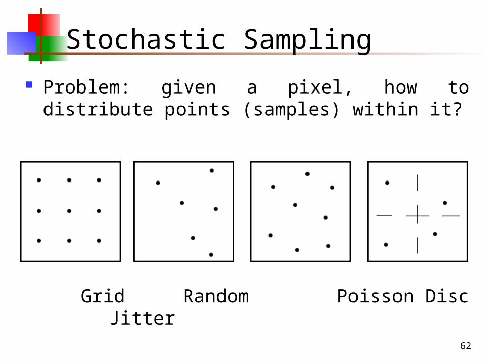
Problem: given a pixel, how to distribute points (samples) within it?
Grid Random Poisson Disc Jitter
63
Stochastic Sampling
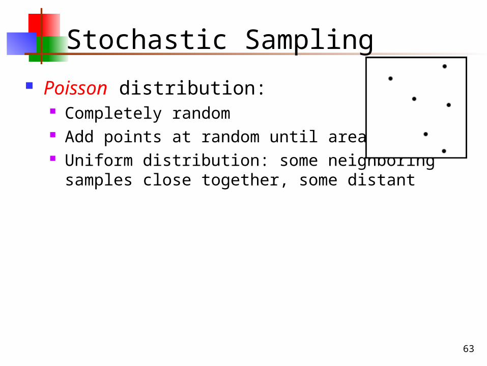
Poisson distribution: Completely random Add points at random until area is full. Uniform distribution: some neighboring
samples close together, some distant
64
Stochastic Sampling
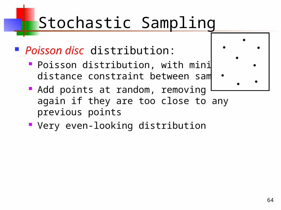
Poisson disc distribution: Poisson distribution, with minimum-
distance constraint between samples Add points at random, removing
again if they are too close to any previous points
Very even-looking distribution
65
Stochastic Sampling
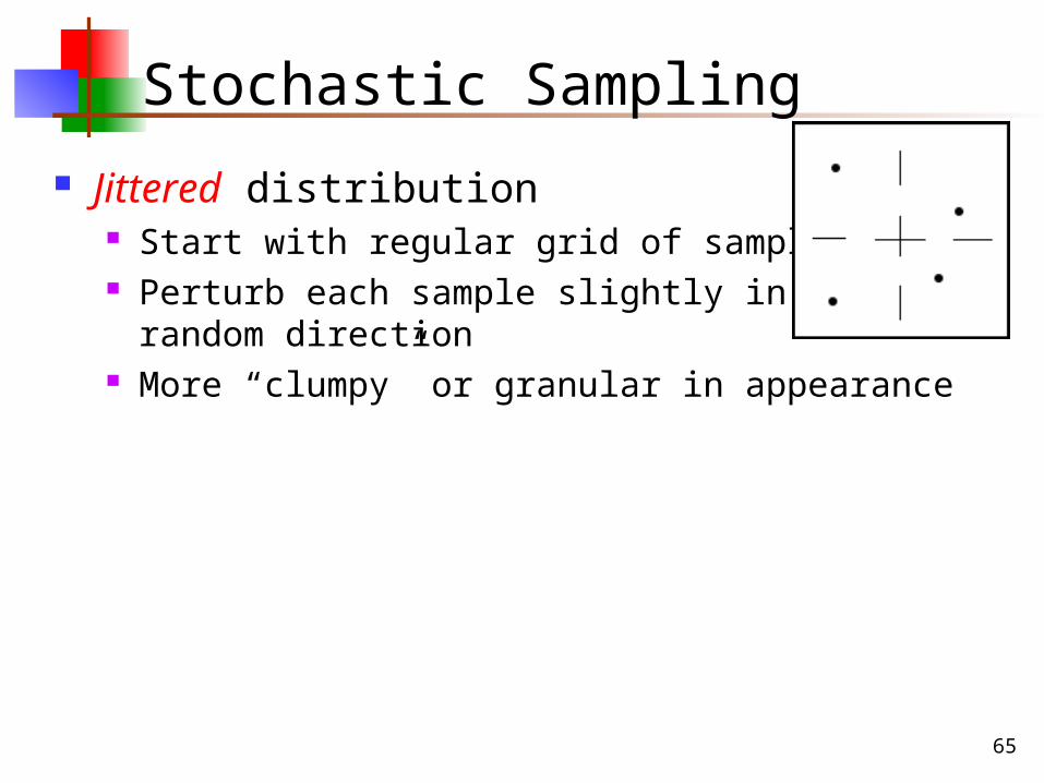
Jittered distribution Start with regular grid of samples Perturb each sample slightly in a
random direction More “clumpy” or granular in appearance
66
Stochastic Sampling
Spectral characteristics of these distributions: Poisson: completely uniform (white noise). High and low
frequencies equally present Poisson disc: Pulse at origin (DC component of image),
surrounded by empty ring (no low frequencies), surrounded by white noise
Jitter: Approximates Poisson disc spectrum, but with a smaller empty disc.
67
Stochastic Sampling
Watt & Watt, p. 134 See Foley & van Dam, p 644-645 Should have images next time