All-scale spatial analysis of ecological data by means of principal ...adn.biol.umontreal.ca/~numericalecology/Reprints/Scale_paper.pdf · the spatial patterns by starting from the

Ecological Modelling 153 (2002) 51–68

All-scale spatial analysis of ecological data by means ofprincipal coordinates of neighbour matrices

Daniel Borcard *, Pierre LegendreDepartement de sciences biologiques, Uni�ersite de Montreal, C.P. 6128, succ. Centre-�ille, Montreal Quebec, Canada H3C 3J7

Abstract

Spatial heterogeneity of ecological structures originates either from the physical forcing of environmental variablesor from community processes. In both cases, spatial structuring plays a functional role in ecosystems. Ecologicalmodels should explicitly take into account the spatial structure of ecosystems. In previous work, we used a polynomialfunction of the geographic coordinates of the sampling sites to model broad-scale spatial variation in a canonical(regression-type) modelling context. In this paper, we propose a method for detecting and quantifying spatial patternsover a wide range of scales. This is obtained by eigenvalue decomposition of a truncated matrix of geographicdistances among the sampling sites. The eigenvectors corresponding to positive eigenvalues are used as spatialdescriptors in regression or canonical analysis. This method can be applied to any set of sites providing a goodcoverage of the geographic sampling area. This paper investigates the behaviour of the method using numericalsimulations and an artificial pseudo-ecological data set of known properties. © 2002 Elsevier Science B.V. All rightsreserved.

Keywords: Geographic distances among sampling sites; Principal coordinate analysis; Variation partitioning; Scale; Spatial analysis

www.elsevier.com/locate/ecolmodel

1. Introduction

In ecological theory, a major paradigm statesthe importance of spatial structure, not only as apotential nuisance for sampling or statistical test-ing, but also as a functional necessity, to bestudied for its own sake and included into ecolog-ical modelling (Legendre and Fortin, 1989; Legen-dre, 1993; Legendre and Legendre, 1998). In theframework of multivariate data analysis, severalmethods have been proposed to include space as

an explicit predictor. Legendre and Troussellier(1988) used a matrix of Euclidean (geographic)distances among their sampling sites in a series ofMantel and partial Mantel tests. Legendre (1990)proposed using geographic coordinates directly asexplanatory variables in constrained ordinationtechniques (redundancy analysis, RDA, andcanonical correspondence analysis, CCA), byplacing the terms of a cubic trend-surface equa-tion into the explanatory (i.e. constraining) datamatrix. This approach, called multivariate trend-surface analysis, was later integrated into amethod of variation partitioning, where ecologicalvariation was decomposed into four fractions(pure environmental, pure spatial, explained both

* Corresponding author. Fax: +1-514-343-2293.E-mail address: [email protected] (D. Bor-

card).

0304-3800/02/$ - see front matter © 2002 Elsevier Science B.V. All rights reserved.

PII: S0 304 -3800 (01 )00501 -4

mailto:[email protected]

D. Borcard, P. Legendre / Ecological Modelling 153 (2002) 51–6852

by space and environment, and unexplained) us-ing partial constrained ordination (Borcard et al.,1992; Borcard and Legendre, 1994; Meot et al.,1998). This technique, which was summarised byLegendre and Legendre (1998), Section 13.5, hasproved very successful and is now widely appliedin various fields of ecology (see references inLegendre and Legendre (1998), p. 775).

The coarseness of trend-surface analysis pre-sents a problem, however. This method is devisedto model broad-scale spatial structures with sim-ple shapes like planes, saddles, or parabolas repre-senting bumps or troughs. Finer structures cannotbe adequately modelled by this method: too manyparameters would be required to do so.

In recent years, researchers have increased theirawareness of the fact that ecological processesoccur at defined scales, and that their perceptiondepends upon a proper matching of the samplingstrategy to the size, grain and extent of the study,and the statistical tools used to analyse the data.This has generated the need for analytical tech-niques devised to reveal the spatial structures of adata set at any scale that can be perceived by thesampling design. In this paper, we propose amethod for detecting and quantifying spatial pat-terns over a wide range of scales. This method canbe applied to any set of sites providing a goodcoverage of the geographic sampling area. Thismethod will first be presented in the unidimen-sional context, where it has the further advantageof being usable even for short (n�25) data series.

2. The method

The analysis begins by coding the spatial infor-mation in a form allowing us to recover variousstructures over the whole range of scales encom-passed by the sampling design. This technique willwork on data sampled along linear transects aswell as on geographic surfaces or in three-dimen-sional space. This paper will focus on the unidi-mensional case, demonstrating the efficiency ofthe method by way of simulations of simple andcomplex data.

In the framework of linear modelling, the moststraightforward technique for modelling spatial

structures is polynomial regression (trend-surfaceanalysis in the bidimensional case), where thespatial variables are used to generate a polyno-mial function of the X (or X and Y, or X, Y andZ) coordinates of the sampling units (Legendre,1990; Borcard et al., 1992; Borcard and Legendre,1994). For a linear transect, using the X coordi-nates of the sampling units as an explanatoryvariable allows one to model a linear trend thatmay be present in the data. Adding a second-or-der (X2) monomial term allows the model to bebent once in the form of a parabola. Each higher-order term generates one more bend, and henceincreases the fit of the model to finer-scale spatialstructures. One major problem with this approachis that the individual terms are highly correlated,thereby preventing the modelling of independentstructures at different scales. Furthermore, espe-cially in the bidimensional case, the number ofterms of the polynomial function grows veryquickly, making the third order (with nine terms)the highest one to be usable practically, despite itscoarseness in terms of spatial resolution. Polyno-mials can be turned into orthogonal polynomials,either by using a Gram–Schmidt orthogonaliza-tion procedure, or by carrying out a principalcomponent analysis (PCA) on the matrix of mo-nomials. A new difficulty arises: each new orthog-onal variable is a linear combination of several (inthe case of the Gram–Schmidt orthogonalization)or all (in the case of PCA) the original variables;it does not represent a single scale any longer. Tosolve these problems, our new approach has adifferent starting point involving the close neigh-bourhood relationships among the sampling sites.

2.1. Modified matrix of Euclidean distances

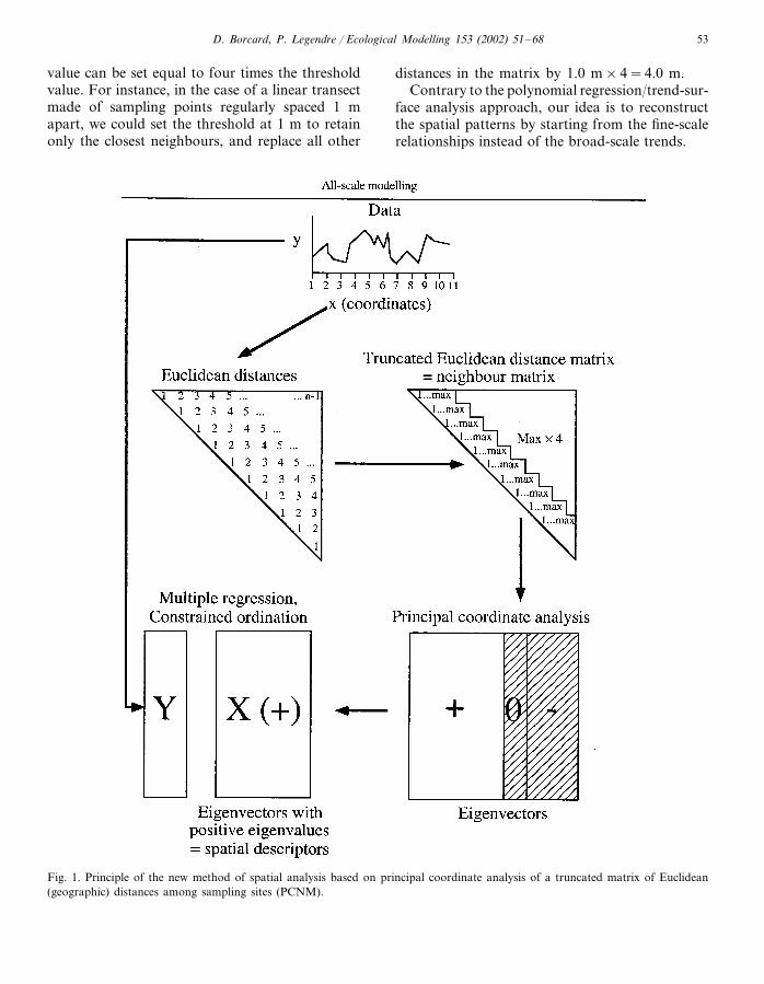
Fig. 1 displays the steps of a complete spatialanalysis using the new method based on principalcoordinates of neighbour matrices (PCNM).

First, we construct a matrix of Euclidean dis-tances among the sites. Then, we define athreshold under which the Euclidean distances arekept as measured, and above which all distancesare considered to be ‘large’, the correspondingnumbers being replaced by an arbitrarily largevalue. For a reason explained later, this large

D. Borcard, P. Legendre / Ecological Modelling 153 (2002) 51–68 53

value can be set equal to four times the thresholdvalue. For instance, in the case of a linear transectmade of sampling points regularly spaced 1 mapart, we could set the threshold at 1 m to retainonly the closest neighbours, and replace all other

distances in the matrix by 1.0 m×4=4.0 m.Contrary to the polynomial regression/trend-sur-

face analysis approach, our idea is to reconstructthe spatial patterns by starting from the fine-scalerelationships instead of the broad-scale trends.

Fig. 1. Principle of the new method of spatial analysis based on principal coordinate analysis of a truncated matrix of Euclidean(geographic) distances among sampling sites (PCNM).


2.2. Principal coordinate analysis

The second step is to compute the principalcoordinates of the modified distance matrix. Thisis necessary because we need our spatial informa-tion to be represented in a form compatible withapplications of multiple regression or canonicalordination (RDA or CCA) i.e. as an object-by-variable matrix. We obtain one or several null,and several negative eigenvalues. Principal coordi-nate analysis of the truncated distance matrixmakes it impossible to represent the distance ma-trix entirely in a space of Euclidean or complexcoordinates. The negative eigenvalues cannot beused as such because the corresponding axes arecomplex (i.e. the coordinates of the sites alongthese axes are complex numbers). In any case, thepositive eigenvalues represent the Euclidean com-ponents of the neighbourhood relationships ofour truncated matrix; these are the componentsthat are of interest to us. Of course, one couldcorrect for the negative eigenvalues using one ofthe methods described in Gower and Legendre(1986) or Legendre and Legendre (1998). Thesemethods consist in adding a constant either to theoriginal non-diagonal distances, or to the squarednon-diagonal distances in the matrix. By doing so,one increases all distances and changes the recon-structed spatial arrangement of the sampling sites.We have empirically compared the results ob-tained using either the original real-number axescorresponding to positive eigenvalues, or all axesafter correction for negative eigenvalues. Resultsindicate that a good reconstruction of the spatialstructures is obtained by using the formermethod, i.e. only the axes corresponding to posi-tive eigenvalues, without correcting the axes hav-ing negative eigenvalues.

The principal coordinates derived from thesepositive eigenvalues can now be used as explana-tory variables in multiple regression, RDA, orCCA, depending on the context.

To investigate the process of truncation of thedistance matrix, explained above, we built a seriesof truncated distance matrices with ‘large dis-tance’ values made of a series of factors rangingfrom 2 to 8. We observed that beyond a factor offour times the threshold for the ‘large’ distances,

the principal coordinates remain the same towithin a multiplicative constant. In other words,the first principal coordinate obtained with a fac-tor of 4 had a correlation of 1.0 with the firstprincipal coordinate obtained with a factor of 5,or any other value; the same was true for thewhole series of principal coordinates. Conse-quently, multiple regressions using principal coor-dinates obtained with a multiplicative constant of4 and above will yield the same R2 and the sameP-values as with any other multiplicative constantlarger than 4. Thus we decided to apply the factor4 in all subsequent steps of our investigation.

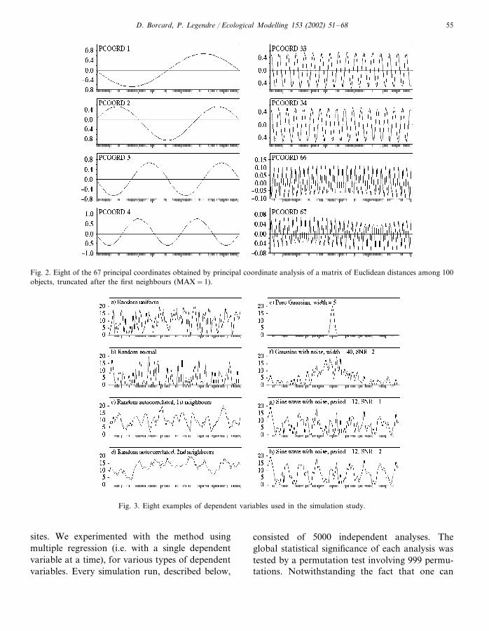
When computed from a distance matrix corre-sponding to n equidistant objects arranged as astraight line, as in Fig. 1, truncated with athreshold of one unit (MAX=1 i.e. only theimmediate neighbours are retained), the principalcoordinates correspond to a series of sinusoidswith decreasing periods (Fig. 2); the largest periodis n+1, and the smallest one is equal to orslightly larger than 3. The number of principalcoordinates is a round integer corresponding totwo-thirds of the number of objects. If the trunca-tion threshold is larger than 1, fewer principalcoordinates are obtained, and several among thelast (finer) ones are distorted, showing aliasing ofstructures having periods too short to be repre-sented adequately by the discrete site coordinates.This behaviour will later be shown to have impor-tant consequences on the performance of themethod. Thus, our method presents a superficialresemblance to Fourier analysis and harmonicregression, but it will be shown to be more generalsince it can model a wider range of signals, andcan be used with irregularly spaced data.

3. Numerical simulations

We conducted extensive simulations to explorethe behaviour of the method regarding type Ierror and power to detect various kinds of signals(Fig. 3); power was measured as the rate of rejec-tion of the null hypothesis, at significance level0.05, when an effect was present in the data. Thesimulation setup consisted of a straight line with100 equidistant points representing the sampling


Fig. 2. Eight of the 67 principal coordinates obtained by principal coordinate analysis of a matrix of Euclidean distances among 100objects, truncated after the first neighbours (MAX=1).

Fig. 3. Eight examples of dependent variables used in the simulation study.

sites. We experimented with the method usingmultiple regression (i.e. with a single dependentvariable at a time), for various types of dependentvariables. Every simulation run, described below,

consisted of 5000 independent analyses. Theglobal statistical significance of each analysis wastested by a permutation test involving 999 permu-tations. Notwithstanding the fact that one can


never simulate all possible or relevant ecologicalsituations, the following results are presented assupport for the sensitivity of the method describedin this paper.

For statistical testing, we used the method ofpermutation of residuals under a full model (terBraak, 1990, 1992; Anderson and Legendre,1999); in this method, the permutable units arethe residuals of the multiple regression. As a teststatistic for the global test, we used the R2 of themultiple regression; within any given permutationtest, the values of R2 and F are monotonic to eachother and, thus, represent equivalent statistics forpermutation testing. In applications on complexdata involving tests of individual regression coeffi-

cients, we also tested by permutation the t-statis-tic associated with each regression coefficient.

3.1. Random �ariables and type I error

The first series of simulations focussed on thetype I error of the method. The dependent vari-ables were random numbers drawn from fourdifferent distributions: uniform (Fig. 3a), normal(Fig. 3b), exponential, and (as an extreme case)exponential cubed, following Manly (1997) andAnderson and Legendre (1999). Fig. 4 shows theresults of these runs, carried out using two differ-ent truncation thresholds (value MAX) of thespatial matrix. Several independent series of 5000

Fig. 4. Type I error of the method (a, b) and percentage of variance explained (R2: c, d) on series of 100 data points randomly drawnfrom four different distributions, with spatial matrices with two different resolutions set by the truncation threshold (value MAX)of the Euclidean distance matrix. Each run consisted of 5000 independent simulations. The error bars in (a) and (b) represent 95%confidence intervals.


simulations showed that the frequency distribu-tion of the P-values was approximately flat (re-sults not illustrated), yielding an appropriatenumber of type I error cases (Fig. 4a and b).Thus, the method showed good performance onthis crucial aspect. Note also the percentage ofvariance ‘explained’ (non-significantly): in linearregression, when the dependent variable is com-pletely random, as it is the case in these simula-tions, the expected value of R2 is equal to theratio between the number of explanatory variablesand the number of objects minus 1. The resultspresented in Fig. 4c and d are right on the spot.

3.2. Power to detect autocorrelation in randomresponse �ariables

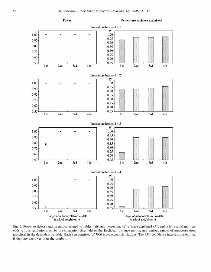
In a second series of simulations, we addedautocorrelation to the random response variables(Fig. 3c and d). After generating a series of ran-dom numbers drawn from a standard normaldistribution, we computed moving averages onthe series, with window widths varying from 3 (i.e.one random value and its first neighbours oneither side) to 9 (one value and its four neigh-bours on either side). The number of neighbours(on one side of a point) that are included in themoving average are used as a measure of therange of the autocorrelation: the window width of3 has a range of 1 while the window width of 9has a range of 4. The results, displayed in Fig. 5,show that the method detected spatial structuresgenerated by autocorrelation almost faultlessly(power=1), provided that the truncation value ofthe spatial matrix was smaller than the windowwidth of the autocorrelation. This is an importantresult which can be related to the number andshape of the principal coordinates described be-fore. Retaining more distant neighbours producedfewer principal coordinates, the ones representingthe finest structures being lost. Besides, the lastpart of the series of principal coordinates, whichshould have contained the sines with the shortestperiods, were distorted if the truncation of thematrix of Euclidean distances retained more thanthe first neighbours. This in turn decreased theability of the set of principal coordinates to detectfine spatial structures in the dependent variables.

As will be shown below, this property of themethod also appears when one looks for othertypes of spatial structures in the dependentvariables.

3.3. Power to detect Gaussian cur�es

The third series of simulations was devoted tothe detection of a single, Gaussian-shaped bump,because species frequencies often have unimodal(Gaussian-like) distributions along environmentgradients (Austin, 1976). A Gaussian function (i.e.a normal density function) was computed, with agiven maximum height and width; the width wasdefined as two standard deviations on either sideof the mean, measured in sampling intervals.Within each simulation run, the width and maxi-mum height were fixed, while the position of themean of the curve along the transect varied atrandom.

A first series of runs involved only a thin Gaus-sian curve (5 sampling intervals wide, Fig. 3e),which was submitted to spatial matrices of in-creasing coarseness (Fig. 6a). These simulationsshowed that the method had no problem in de-tecting the signal, provided that the threshold ofthe spatial matrix was lower than or equal to thewidth of the Gaussian curve. The percentage ofvariance explained varied, though, increasingwhen the spatial matrix allowed finer resolutioni.e. when the truncation value tended to 1 (Fig.6b).

In another series of runs, normal noise wasadded to the Gaussian curve (Fig. 3f) with asignal-to-noise ratio (SNR) arbitrarily defined asthe maximum height of the Gaussian curve di-vided by twice the standard deviation of the noise.With this definition, a SNR equal to 1 implies anormal noise component where 68% of the ran-dom values fall within a range equal to the maxi-mum height chosen for the Gaussian curve. Thedata generation algorithm was the following:1. Generate a Gaussian curve with a known max-

imum height MH (for instance MH=20).2. Draw random values from a normal distribu-

tion with mean=0 and standard deviation=1.

3. Select a SNR (for instance SNR=2).


Fig. 5. Power to detect random autocorrelated variables (left) and percentage of variance explained (R2: right) for spatial matriceswith various resolutions, set by the truncation threshold of the Euclidean distance matrix, and various ranges of autocorrelation(abscissa) in the dependent variable. Each run consisted of 5000 independent simulations. The 95% confidence intervals are omittedif they are narrower than the symbols.


Fig. 6. Power to detect Gaussian-shaped bumps (a) and percentage of variance explained (R2: b) for spatial matrices with variousresolutions set by the truncation threshold of the Euclidean distance matrix (abscissa). Each run consisted of 5000 independentsimulations. The 95% confidence intervals are omitted if they are narrower than the symbols. In the absence of noise in the data,the variation in the results (shown by the error bars) are due to some dependence of the power to the position of the Gaussian bumpin the data series.

4. Adjust the standard deviation of the noise bymultiplying its values by MH/(SNR×2); thisworks because multiplying the values of arandom normal series by a given number mul-tiplies its standard deviation by that number.In our example: noise SD=20/(2×2)=5, somultiply all values obtained in (2) by 5.

5. Add signal (obtained in (1)) and noise (ob-tained in (4)).

6. Set all negative values of the data obtained in(5) to zero. Because they simulate species dis-tributions, these values cannot be negative.

7. Rescale the data so obtained to the pre-se-lected maximum height.

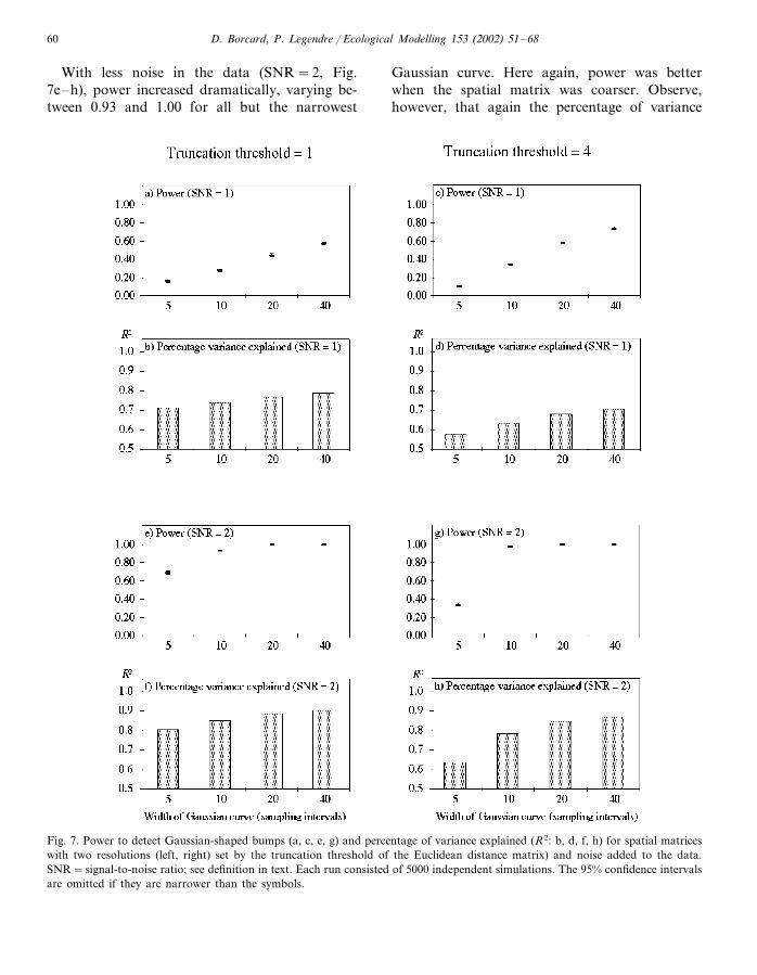
Fig. 7 shows that the capacity of detection ofthe method depended on both the SNR and thewidth of the Gaussian curve. With SNR=1 (Fig.7a–d), power was 0.74 in the best case. Thisoccurred with the broadest curve (40 samplingintervals) and, interestingly, the coarsest spatialmatrix (truncation threshold=4: Fig. 7d). Thisfeature, better power obtained when using acoarser spatial matrix, held true for all but thenarrowest Gaussian curve. The coarseness of thespatial matrix seemed to allow it to ‘see’ throughthe noise better than finer ones. As expected, thebroader the Gaussian curve, the easier its detec-tion is by our method.


With less noise in the data (SNR=2, Fig.7e–h), power increased dramatically, varying be-tween 0.93 and 1.00 for all but the narrowest

Gaussian curve. Here again, power was betterwhen the spatial matrix was coarser. Observe,however, that again the percentage of variance

Fig. 7. Power to detect Gaussian-shaped bumps (a, c, e, g) and percentage of variance explained (R2: b, d, f, h) for spatial matriceswith two resolutions (left, right) set by the truncation threshold of the Euclidean distance matrix) and noise added to the data.SNR=signal-to-noise ratio; see definition in text. Each run consisted of 5000 independent simulations. The 95% confidence intervalsare omitted if they are narrower than the symbols.


explained was higher when the spatial matrix wasfiner (truncation threshold=1); this is a logicalresult considering that finer explanatory variablescan model finer structures in the data.

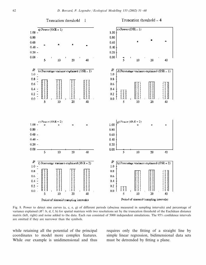
3.4. Power to detect sine cur�es

A fourth series of simulations was devoted tosinusoids, with periods varying from 5 to 40 inter-site distances, and SNR having values of 1 (Fig.3g) and 2 (Fig. 3h). The results, shown in Fig. 8,bear some resemblance with those obtained forGaussian curves: power depended on the amountof noise in the data (compare Fig. 8a–e and Fig.8c–g), and more variance was explained when thespatial matrices were finer (truncationthreshold=1; compare Fig. 8b–d and Fig. 8f–h).Interestingly and predictably, the finest sinusoidswere never detected when the spatial matrix wastoo coarse (Fig. 8c–g, periods of 5). In that case,the period of the finest spatial principal coordi-nate was larger than that of the dependent vari-able. Another noteworthy feature is that, contraryto the Gaussian case, the amount of varianceexplained did not vary with the period of thesinusoid for given combinations of SNR and spa-tial matrix resolution, provided that the latter wasfine enough to detect the signal. When this wasnot the case, no combination of the availablevariables could adequately model the dependentvariable.

3.5. Power to detect gradients

Our last series of simulations focussed on lineargradients with SNR values of 1 and 2. Strikingly,the method never failed to detect the pattern, andalways explained practically all the variance; theproportion of the dependent variable’s varianceexplained was between 0.998 and 0.999.

4. Test on complex data

This section is devoted to the illustration of theuse of our method with actual data sets. Ourexample involves artificial data constructed by

combining various kinds of signals usually presentin real data, plus two types of noise. This providesa pattern that has the double advantage of beingrealistic and controlled, thereby permitting a pre-cise assessment of the potential of the method torecover the structured part of the signal and todissect it into its primary components. Other pa-pers will be devoted to the application of themethod to real ecological data sets.

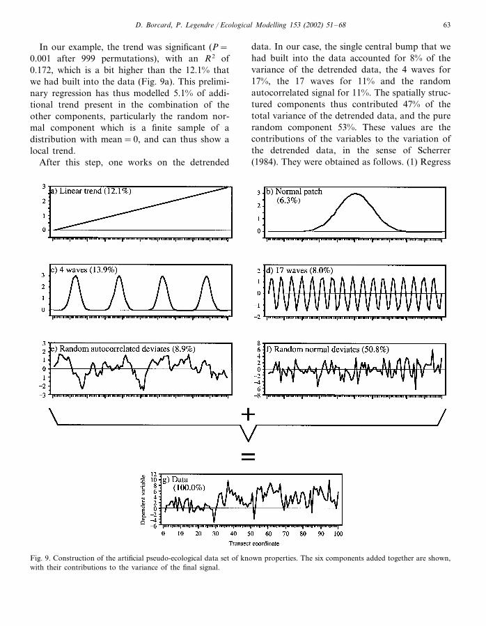
4.1. The data

We constructed the data by adding the follow-ing components together (Fig. 9) into a transectconsisting of 100 equidistant observations:1. a linear trend (Fig. 9a);2. a single normal patch in the centre of the

transect (Fig. 9b);3. four waves (i.e. a sine wave with a period of 25

sampling units) (Fig. 9c);4. 17 waves (i.e. a sine wave with a period of

�5.9 sampling units) (Fig. 9d);5. a random autocorrelated variable, with auto-

correlation determined by a spherical vari-ogram with nugget value=0 and range=5(Fig. 9e);

6. a noise component drawn from a randomnormal distribution with mean=0 and vari-ance=4 (Fig. 9f).

Fig. 9 shows the partial contributions of the sixcomponents to the variance of the final artificialresponse variable. The random noise (Fig. 9f)contributed for more than half of the total vari-ance. Thus, the spatially structured componentsof the compound signal (Fig. 9a–e) were wellhidden in the noise, as it is often the case with realecological data.

4.2. Analytical procedure

4.2.1. Detrending the dependent �ariableAs it is the case in most techniques of spatial

analysis, the first step is to detrend the data. Werecommend doing it whenever a significant lineartrend is detected even though our method is ableto model linear trends, because this preliminarystep allows a separate modelling of the trend


Fig. 8. Power to detect sine curves (a, c, e, g) of different periods (abscissa measured in sampling intervals) and percentage ofvariance explained (R2: b, d, f, h) for spatial matrices with two resolutions set by the truncation threshold of the Euclidean distancematrix (left, right) and noise added to the data. Each run consisted of 5000 independent simulations. The 95% confidence intervalsare omitted if they are narrower than the symbols.

while retaining all the potential of the principalcoordinates to model more complex features.While our example is unidimensional and thus

requires only the fitting of a straight line bysimple linear regression, bidimensional data setsmust be detrended by fitting a plane.


In our example, the trend was significant (P=0.001 after 999 permutations), with an R2 of0.172, which is a bit higher than the 12.1% thatwe had built into the data (Fig. 9a). This prelimi-nary regression has thus modelled 5.1% of addi-tional trend present in the combination of theother components, particularly the random nor-mal component which is a finite sample of adistribution with mean=0, and can thus show alocal trend.

After this step, one works on the detrended

data. In our case, the single central bump that wehad built into the data accounted for 8% of thevariance of the detrended data, the 4 waves for17%, the 17 waves for 11% and the randomautocorrelated signal for 11%. The spatially struc-tured components thus contributed 47% of thetotal variance of the detrended data, and the purerandom component 53%. These values are thecontributions of the variables to the variation ofthe detrended data, in the sense of Scherrer(1984). They were obtained as follows. (1) Regress

Fig. 9. Construction of the artificial pseudo-ecological data set of known properties. The six components added together are shown,with their contributions to the variance of the final signal.


the detrended data on the central bump, 4 waves,17 waves, random autocorrelated and randomsignals originally built into the data. (2) Computethe correlation of each variable with the de-trended data. (3) Compute each contribution asthe product of the standardised (partial) regres-sion coefficient with the correlation coefficient.These contributions will be compared later withthe structures revealed by the PCNM method.

4.2.2. Building the matrix of spatial �ariablesThis step involves the procedure described in

Section 2: build a matrix of Euclidean distancesamong objects, truncate it to the first neighbours,replace the removed values by the highest valueretained multiplied by 4, and compute the princi-pal coordinates of the resulting matrix. Our exam-ple being built upon the same linear transect of100 objects as the one used in the simulations, theresults were the same: we obtained 67 principalcoordinates representing a series of sine waves ofdecreasing periods, starting from a period of 101,and ending with a period slightly larger than 3.These are the spatial variables that will be used inthe next steps.

4.2.3. Running the spatial analysisSince our example involves a single dependent

variable, the spatial analysis consists in a multiplelinear regression of the detrended dependent vari-able onto the 67 spatial variables built in step 2.The main question at this step is to decide whatkind of model is appropriate: a global one, retain-ing all the spatial variables and yielding an R2 ashigh as possible, or a more parsimonious modelbased on the most significant spatial variables?The answer may depend on the problem, but inour opinion the general procedure should includesome sort of thinning of the model. Rememberthat the number of parameters of the globalmodel is equal to about 67% of the number ofobjects, a situation which may often lead to anoverstated value of R2 by chance alone. Thesolution that we propose, and have applied to thisexample, consists in testing the significance of allthe (partial) regression coefficients and retainingonly the principal coordinates that are significantat a predetermined (one-tailed) probability value.

All tests can be done using a single series ofpermutations if the permutable units are the resid-uals of a full model (Anderson and Legendre,1999; Legendre and Legendre 1998), which is thecase here. The explanatory variables being orthog-onal, no recomputation of the coefficients of the‘minimum’ model are necessary. Note, however,that a new series of statistical tests based upon theminimum model would give different results, sincethe denominator (residual mean square) of the Fstatistic would have changed.

The analysis of our detrended artificial datayielded a complete model explaining 75.3% of thevariance when using the 67 explanatory variables.Reducing the model as described above allowedus to retain 8 spatial variables at P=0.05, ex-plaining together 43.3% of the variance. Thisvalue compares well with the 47% of the variancerepresenting the contributions of the single bump,the two variables with 4 and 17 waves, and therandom autocorrelated component of the de-trended data. The spatial variables retained wereprincipal coordinates no. 2, 6, 8, 14, 28, 33, 35and 41.

4.2.4. Dissecting the spatial modelOne major advantage of our method is that the

components of the spatial model obtained areorthogonal, and can thus be either examined sepa-rately or combined at will into independent sub-models that can be interpreted with the help ofexternal information. When such knowledge isnot available, the submodels may help generatehypotheses about the underlying processes thathave generated the structures.

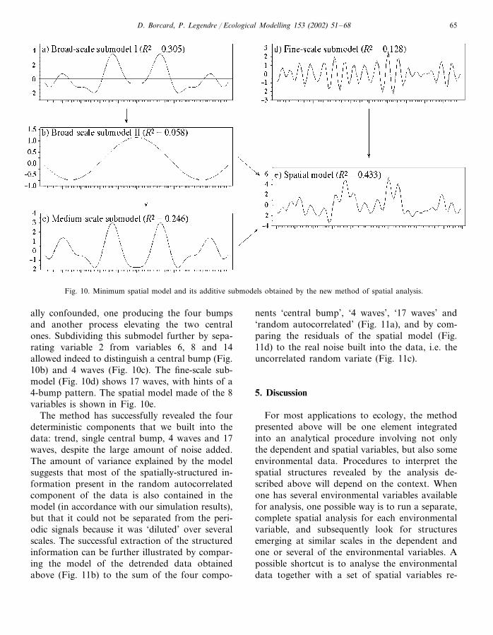
It often happens that the significant variablesare grouped in series of roughly similar periods.In our example, for instance, there is a clear gapbetween the first four significant variables and thelast four. Thus, a first step may be to draw twosubmodels, one involving variables 2, 6, 8 and 14(added together, using their regression coefficientsas weights) and the other involving variables 28,33, 35 and 41. The results are shown in Fig.10a–d, respectively. The ‘broad-scale’ submodel(Fig. 10a) shows 4 major bumps, the two centralones being much higher than the two lateral ones.This may indicate that two mechanisms are actu-


Fig. 10. Minimum spatial model and its additive submodels obtained by the new method of spatial analysis.

ally confounded, one producing the four bumpsand another process elevating the two centralones. Subdividing this submodel further by sepa-rating variable 2 from variables 6, 8 and 14allowed indeed to distinguish a central bump (Fig.10b) and 4 waves (Fig. 10c). The fine-scale sub-model (Fig. 10d) shows 17 waves, with hints of a4-bump pattern. The spatial model made of the 8variables is shown in Fig. 10e.

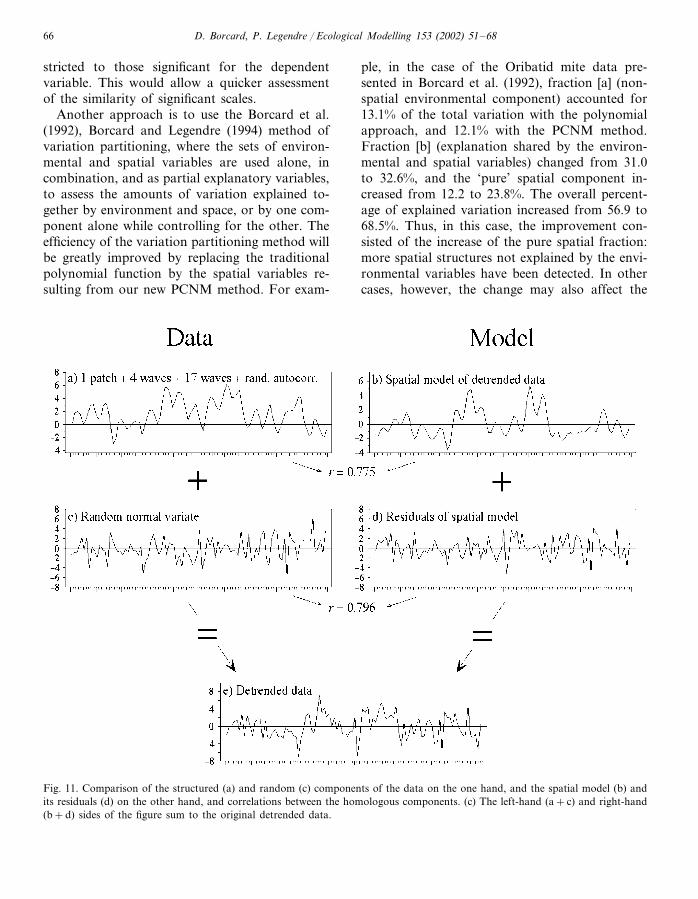
The method has successfully revealed the fourdeterministic components that we built into thedata: trend, single central bump, 4 waves and 17waves, despite the large amount of noise added.The amount of variance explained by the modelsuggests that most of the spatially-structured in-formation present in the random autocorrelatedcomponent of the data is also contained in themodel (in accordance with our simulation results),but that it could not be separated from the peri-odic signals because it was ‘diluted’ over severalscales. The successful extraction of the structuredinformation can be further illustrated by compar-ing the model of the detrended data obtainedabove (Fig. 11b) to the sum of the four compo-

nents ‘central bump’, ‘4 waves’, ‘17 waves’ and‘random autocorrelated’ (Fig. 11a), and by com-paring the residuals of the spatial model (Fig.11d) to the real noise built into the data, i.e. theuncorrelated random variate (Fig. 11c).

5. Discussion

For most applications to ecology, the methodpresented above will be one element integratedinto an analytical procedure involving not onlythe dependent and spatial variables, but also someenvironmental data. Procedures to interpret thespatial structures revealed by the analysis de-scribed above will depend on the context. Whenone has several environmental variables availablefor analysis, one possible way is to run a separate,complete spatial analysis for each environmentalvariable, and subsequently look for structuresemerging at similar scales in the dependent andone or several of the environmental variables. Apossible shortcut is to analyse the environmentaldata together with a set of spatial variables re-


stricted to those significant for the dependentvariable. This would allow a quicker assessmentof the similarity of significant scales.

Another approach is to use the Borcard et al.(1992), Borcard and Legendre (1994) method ofvariation partitioning, where the sets of environ-mental and spatial variables are used alone, incombination, and as partial explanatory variables,to assess the amounts of variation explained to-gether by environment and space, or by one com-ponent alone while controlling for the other. Theefficiency of the variation partitioning method willbe greatly improved by replacing the traditionalpolynomial function by the spatial variables re-sulting from our new PCNM method. For exam-

ple, in the case of the Oribatid mite data pre-sented in Borcard et al. (1992), fraction [a] (non-spatial environmental component) accounted for13.1% of the total variation with the polynomialapproach, and 12.1% with the PCNM method.Fraction [b] (explanation shared by the environ-mental and spatial variables) changed from 31.0to 32.6%, and the ‘pure’ spatial component in-creased from 12.2 to 23.8%. The overall percent-age of explained variation increased from 56.9 to68.5%. Thus, in this case, the improvement con-sisted of the increase of the pure spatial fraction:more spatial structures not explained by the envi-ronmental variables have been detected. In othercases, however, the change may also affect the

Fig. 11. Comparison of the structured (a) and random (c) components of the data on the one hand, and the spatial model (b) andits residuals (d) on the other hand, and correlations between the homologous components. (c) The left-hand (a+c) and right-hand(b+d) sides of the figure sum to the original detrended data.


other components. For instance, the detectionof fine spatial structures also explained bythe environmental variables would increase theshare of component [b] at the expense of fraction[a].

These considerations open the door to applica-tions of the PCNM method to multivariate data.In this case the multiple regression used above isreplaced by a method of constrained ordinationsuitable to the data: RDA (Rao, 1964), CCA (terBraak, 1986), or redundancy analysis on trans-formed species data (Legendre and Gallagher,2001). For these applications, however, no exist-ing program provides the appropriate statisticaltests on individual regression or canonical coeffi-cients to allow the selection of a proper subset ofspatial variables. One would have to rely uponmore traditional, non-permutational tests for ap-proximate results, or on stepwise procedures. Thet-values of regression coefficients provided by theprogram Canoco (ter Braak and Smilauer, 1998)can also be used for assessment of the mostimportant spatial variables, although they are notaccompanied by permutational probabilities. Inthe future, programs of canonical analysis shouldinclude permutational tests of significance of indi-vidual regression coefficients.

Another possible extension concerns data sam-pled across a surface i.e. bidimensional spatialdata. Preliminary attempts in this direction showthat our method still provides periodic spatialvariables if the data are regular, but that thespatial resolution is about half that obtained inthe unidimensional case; the bidimensional modelincludes the same number of principal coordi-nates as the unidimensional. Besides, the princi-pal coordinates do not show the simplescale-to-variance relationship which allows themto appear readily in decreasing order of periodsin the unidimensional case.

Finally, a word must be said about irregularlysampled data. The effect of a missing data pointin a regular series is to disrupt the sine wavesprovided by the principal coordinate analysis.This disruption acts on the amplitude, phase andperiod of the sines, thereby affecting the interpre-tation of the spatial variables in terms of scales.Truly irregular sampling patterns result in totally

irregular principal coordinates. Note that theseare still suitable spatial descriptors, but their in-terpretation is complicated by the fact that eachone of them often bears structures at severalscales.

In cases where a regular sampling series suffersfrom one or a few missing observations, there is asimple way of overcoming the problem. It con-sists in filling the voids i.e. adding points wherethey are missing in the file of spatial coordinates;nothing is added or interpolated in the dependentvariable. The filled-up series is then submitted tothe analysis yielding the principal coordinates,and then the supplementary objects are removedfrom the matrix of principal coordinates before itis used as a set of spatial explanatory variables.This trick has a cost, however: removal of thesupplementary objects introduces some correla-tion among the spatial variables, which were pre-viously uncorrelated. As long as the number ofsupplementary objects remains low in comparisonto the number of observed objects, these correla-tions are low. But an exaggerated use of supple-mentary objects may introduce unwantedamounts of correlation among the spatial vari-ables, thereby compromising one major feature ofthe method, i.e. the independence of the spatialvariables, which is required for their combinationinto orthogonal submodels.

This paper raises a number of mathematicalquestions; for instance, the relationship betweenour method of decomposition of the spatial rela-tionships among sites and the one proposed byMeot et al. (1993), Fourier analysis, and the de-composition of Toeplitz matrices. We hope thatthe paper will attract the interest of mathemati-cians who can help us understand these proper-ties and develop methods of spatial modellingfurther.

A FORTRAN program (SPACEMAKER: sourcecode, compiled versions for Macintosh and DOS,and program documentation) to carry out theprincipal coordinate decomposition of spatial lo-cations described in this paper is available on theWWWeb site http://www.fas.umontreal.ca/biol/legendre/ or via anonymous ftp at ftp://ftp.umontreal.ca/pub/casgrain/labo/SPACEMAKER

/.

http://www.fas.umontreal.ca/biol/legendre/

http://www.fas.umontreal.ca/biol/legendre/

ftp://ftp.umontreal.ca/pub/casgrain/labo/SpaceMaker/




Acknowledgements

This paper is dedicated to F. James Rohlf onthe occasion of his 65th birthday. This researchwas supported by NSERC grant no. OGP7738 toP. Legendre. We thank also two anonymous re-viewers for their helpful comments.

References

Anderson, M.J., Legendre, P., 1999. An empirical comparisonof permutation methods for tests of partial regressioncoefficients in a linear model. J. Statist. Comput. Simul. 62,271–303.

Austin, M.P., 1976. On nonlinear species response models inordination. Vegetatio 33, 33–41.

Borcard, D., Legendre, P., Drapeau, P., 1992. Partialling outthe spatial component of ecological variation. Ecology 73,1045–1055.

Borcard, D., Legendre, P., 1994. Environmental control andspatial structure in ecological communities: an exampleusing Oribatid mites (Acari, Oribatei). Environ. Ecol. Stat.1, 37–61.

Gower, J.C., Legendre, P., 1986. Metric and Euclidean proper-ties of dissimilarity coefficients. J. Classif. 3, 5–48.

Legendre, P., 1990. Quantitative methods and biogeographicanalysis. In: Garbary, D.J., South, R.G. (Eds.), Evolution-ary biogeography of the marine algae of the North At-lantic. NATO ASI Series, vol. G 22. Springer-Verlag,Berlin, pp. 9–34.

Legendre, P., 1993. Spatial autocorrelation: trouble or newparadigm? Ecology 74, 1659–1673.

Legendre, P., Fortin, M.-J., 1989. Spatial pattern and ecologi-cal analysis. Vegetatio 80, 107–138.

Legendre, P., Gallagher, E.D., 2001. Ecologically meaningfultransformations for ordination of species data. Oecologia,129, 271–280.

Legendre, P., Legendre, L., 1998. Numerical ecology, secondEnglish ed. Elsevier Science BV, Amsterdam, p. 853.

Legendre, P., Troussellier, M., 1988. Aquatic heterotrophicbacteria: modeling in the presence of spatial autocorrela-tion. Limnol. Oceanogr. 33, 1055–1067.

Manly, B.J.F., 1997. Randomization, bootstrap and MonteCarlo methods in biology, second ed. Chapman and Hall,London, p. 399.

Meot, A., Chessel, D., Sabatier, R., 1993. Operateurs devoisinage et analyse des donnees spatio-temporelles. In:Lebreton, J.D., Asselain, B. (Eds.), Biometrie et environ-nement. Masson, Paris, pp. 46–71.

Meot, A., Legendre, P., Borcard, D., 1998. Partialling out thespatial component of ecological variation: questions andpropositions in the linear modeling framework. Environ.Ecol. Stat. 5, 1–26.

Rao, C.R., 1964. The use and interpretation of principalcomponent analysis in applied research. Sankhyaa A 26,329–358.

Scherrer, B., 1984. Biostatistique. Gaetan Morin, Chicoutimi,pp. 850.

ter Braak, C.J.F., 1986. Canonical correspondence analysis: anew eigenvector technique for multivariate direct gradientanalysis. Ecology 67, 1176–1179.

ter Braak, C.J.F., 1990. Update notes: CANOCO version 3.10.Agricultural Mathematics Group, Wageningen.

ter Braak, C.J.F., 1992. Permutation versus bootstrap signifi-cance tests in multiple regression and ANOVA. In: Jockel,K.-H., Rothe, G., Sendler, W. (Eds.), Bootstrapping andrelated techniques. Springer, Berlin, pp. 79–86.

ter Braak, C.J.F. and Smilauer, P., 1998. CANOCO referencemanual and user’s guide to Canoco for Windows—Soft-ware for canonical community ordination (version 4). Mi-crocomputer Power, Ithaca, New York, pp. 351.

Documents

All-scale spatial analysis of ecological data by means of principal ...adn.biol.umontreal.ca/~numericalecology/Reprints/Scale_paper.pdf · the spatial patterns by starting from the