Embed Size (px)
Citation preview
LIGO-P060010-05-Z
All-sky search for periodic gravitational waves in LIGO S4 data
B. Abbott,14 R. Abbott,14 R. Adhikari,14 J. Agresti,14 P. Ajith,2 B. Allen,2, 51 R. Amin,18 S. B. Anderson,14
W. G. Anderson,51 M. Arain,39 M. Araya,14 H. Armandula,14 M. Ashley,4 S. Aston,38 P. Aufmuth,36 C. Aulbert,1
S. Babak,1 S. Ballmer,14 H. Bantilan,8 B. C. Barish,14 C. Barker,15 D. Barker,15 B. Barr,40 P. Barriga,50
M. A. Barton,40 K. Bayer,17 K. Belczynski,24 J. Betzwieser,17 P. T. Beyersdorf,27 B. Bhawal,14 I. A. Bilenko,21
G. Billingsley,14 R. Biswas,51 E. Black,14 K. Blackburn,14 L. Blackburn,17 D. Blair,50 B. Bland,15 J. Bogenstahl,40
L. Bogue,16 R. Bork,14 V. Boschi,14 S. Bose,52 P. R. Brady,51 V. B. Braginsky,21 J. E. Brau,43 M. Brinkmann,2
A. Brooks,37 D. A. Brown,14, 6 A. Bullington,30 A. Bunkowski,2 A. Buonanno,41 O. Burmeister,2 D. Busby,14
R. L. Byer,30 L. Cadonati,17 G. Cagnoli,40 J. B. Camp,22 J. Cannizzo,22 K. Cannon,51 C. A. Cantley,40
J. Cao,17 L. Cardenas,14 M. M. Casey,40 G. Castaldi,46 C. Cepeda,14 E. Chalkey,40 P. Charlton,9 S. Chatterji,14
S. Chelkowski,2 Y. Chen,1 F. Chiadini,45 D. Chin,42 E. Chin,50 J. Chow,4 N. Christensen,8 J. Clark,40 P. Cochrane,2
T. Cokelaer,7 C. N. Colacino,38 R. Coldwell,39 R. Conte,45 D. Cook,15 T. Corbitt,17 D. Coward,50 D. Coyne,14
J. D. E. Creighton,51 T. D. Creighton,14 R. P. Croce,46 D. R. M. Crooks,40 A. M. Cruise,38 A. Cumming,40
J. Dalrymple,31 E. D’Ambrosio,14 K. Danzmann,36, 2 G. Davies,7 D. DeBra,30 J. Degallaix,50 M. Degree,30
T. Demma,46 V. Dergachev,42 S. Desai,32 R. DeSalvo,14 S. Dhurandhar,13 M. Dıaz,33 J. Dickson,4 A. Di Credico,31
G. Diederichs,36 A. Dietz,7 E. E. Doomes,29 R. W. P. Drever,5 J.-C. Dumas,50 R. J. Dupuis,14 J. G. Dwyer,10
P. Ehrens,14 E. Espinoza,14 T. Etzel,14 M. Evans,14 T. Evans,16 S. Fairhurst,7, 14 Y. Fan,50 D. Fazi,14 M. M. Fejer,30
L. S. Finn,32 V. Fiumara,45 N. Fotopoulos,51 A. Franzen,36 K. Y. Franzen,39 A. Freise,38 R. Frey,43 T. Fricke,44
P. Fritschel,17 V. V. Frolov,16 M. Fyffe,16 V. Galdi,46 J. Garofoli,15 I. Gholami,1 J. A. Giaime,16, 18 S. Giampanis,44
K. D. Giardina,16 K. Goda,17 E. Goetz,42 L. M. Goggin,14 G. Gonzalez,18 S. Gossler,4 A. Grant,40 S. Gras,50
C. Gray,15 M. Gray,4 J. Greenhalgh,26 A. M. Gretarsson,11 R. Grosso,33 H. Grote,2 S. Grunewald,1 M. Guenther,15
R. Gustafson,42 B. Hage,36 D. Hammer,51 C. Hanna,18 J. Hanson,16 J. Harms,2 G. Harry,17 E. Harstad,43
T. Hayler,26 J. Heefner,14 I. S. Heng,40 A. Heptonstall,40 M. Heurs,2 M. Hewitson,2 S. Hild,36 E. Hirose,31
D. Hoak,16 D. Hosken,37 J. Hough,40 E. Howell,50 D. Hoyland,38 S. H. Huttner,40 D. Ingram,15 E. Innerhofer,17
M. Ito,43 Y. Itoh,51 A. Ivanov,14 D. Jackrel,30 B. Johnson,15 W. W. Johnson,18 D. I. Jones,47 G. Jones,7 R. Jones,40
L. Ju,50 P. Kalmus,10 V. Kalogera,24 D. Kasprzyk,38 E. Katsavounidis,17 K. Kawabe,15 S. Kawamura,23
F. Kawazoe,23 W. Kells,14 D. G. Keppel,14 F. Ya. Khalili,21 C. Kim,24 P. King,14 J. S. Kissel,18 S. Klimenko,39
K. Kokeyama,23 V. Kondrashov,14 R. K. Kopparapu,18 D. Kozak,14 B. Krishnan,1 P. Kwee,36 P. K. Lam,4
M. Landry,15 B. Lantz,30 A. Lazzarini,14 B. Lee,50 M. Lei,14 J. Leiner,52 V. Leonhardt,23 I. Leonor,43
K. Libbrecht,14 P. Lindquist,14 N. A. Lockerbie,48 M. Longo,45 M. Lormand,16 M. Lubinski,15 H. Luck,36, 2
B. Machenschalk,1 M. MacInnis,17 M. Mageswaran,14 K. Mailand,14 M. Malec,36 V. Mandic,14 S. Marano,45
S. Marka,10 J. Markowitz,17 E. Maros,14 I. Martin,40 J. N. Marx,14 K. Mason,17 L. Matone,10 V. Matta,45
N. Mavalvala,17 R. McCarthy,15 D. E. McClelland,4 S. C. McGuire,29 M. McHugh,20 K. McKenzie,4
J. W. C. McNabb,32 S. McWilliams,22 T. Meier,36 A. Melissinos,44 G. Mendell,15 R. A. Mercer,39
S. Meshkov,14 E. Messaritaki,14 C. J. Messenger,40 D. Meyers,14 E. Mikhailov,17 S. Mitra,13 V. P. Mitrofanov,21
G. Mitselmakher,39 R. Mittleman,17 O. Miyakawa,14 S. Mohanty,33 G. Moreno,15 K. Mossavi,2 C. MowLowry,4
A. Moylan,4 D. Mudge,37 G. Mueller,39 S. Mukherjee,33 H. Muller-Ebhardt,2 J. Munch,37 P. Murray,40 E. Myers,15
J. Myers,15 T. Nash,14 G. Newton,40 A. Nishizawa,23 K. Numata,22 B. O’Reilly,16 R. O’Shaughnessy,24
D. J. Ottaway,17 H. Overmier,16 B. J. Owen,32 Y. Pan,41 M. A. Papa,1, 51 V. Parameshwaraiah,15 P. Patel,14
M. Pedraza,14 S. Penn,12 V. Pierro,46 I. M. Pinto,46 M. Pitkin,40 H. Pletsch,2 M. V. Plissi,40 F. Postiglione,45
R. Prix,1 V. Quetschke,39 F. Raab,15 D. Rabeling,4 H. Radkins,15 R. Rahkola,43 N. Rainer,2 M. Rakhmanov,32
M. Ramsunder,32 K. Rawlins,17 S. Ray-Majumder,51 V. Re,38 H. Rehbein,2 S. Reid,40 D. H. Reitze,39 L. Ribichini,2
R. Riesen,16 K. Riles,42 B. Rivera,15 N. A. Robertson,14, 40 C. Robinson,7 E. L. Robinson,38 S. Roddy,16
A. Rodriguez,18 A. M. Rogan,52 J. Rollins,10 J. D. Romano,7 J. Romie,16 R. Route,30 S. Rowan,40 A. Rudiger,2
L. Ruet,17 P. Russell,14 K. Ryan,15 S. Sakata,23 M. Samidi,14 L. Sancho de la Jordana,35 V. Sandberg,15
V. Sannibale,14 S. Saraf,25 P. Sarin,17 B. S. Sathyaprakash,7 S. Sato,23 P. R. Saulson,31 R. Savage,15 P. Savov,6
S. Schediwy,50 R. Schilling,2 R. Schnabel,2 R. Schofield,43 B. F. Schutz,1, 7 P. Schwinberg,15 S. M. Scott,4
A. C. Searle,4 B. Sears,14 F. Seifert,2 D. Sellers,16 A. S. Sengupta,7 P. Shawhan,41 D. H. Shoemaker,17 A. Sibley,16
J. A. Sidles,49 X. Siemens,14, 6 D. Sigg,15 S. Sinha,30 A. M. Sintes,35, 1 B. J. J. Slagmolen,4 J. Slutsky,18
J. R. Smith,2 M. R. Smith,14 K. Somiya,2, 1 K. A. Strain,40 D. M. Strom,43 A. Stuver,32 T. Z. Summerscales,3
K.-X. Sun,30 M. Sung,18 P. J. Sutton,14 H. Takahashi,1 D. B. Tanner,39 M. Tarallo,14 R. Taylor,14 R. Taylor,40
J. Thacker,16 K. A. Thorne,32 K. S. Thorne,6 A. Thuring,36 K. V. Tokmakov,40 C. Torres,33 C. Torrie,40
G. Traylor,16 M. Trias,35 W. Tyler,14 D. Ugolini,34 C. Ungarelli,38 K. Urbanek,30 H. Vahlbruch,36
arX
iv:0
708.
3818
v1 [
gr-q
c] 2
8 A
ug 2
007
M. Vallisneri,6 C. Van Den Broeck,7 M. Varvella,14 S. Vass,14 A. Vecchio,38 J. Veitch,40 P. Veitch,37 A. Villar,14
C. Vorvick,15 S. P. Vyachanin,21 S. J. Waldman,14 L. Wallace,14 H. Ward,40 R. Ward,14 K. Watts,16
D. Webber,14 A. Weidner,2 M. Weinert,2 A. Weinstein,14 R. Weiss,17 S. Wen,18 K. Wette,4 J. T. Whelan,1
D. M. Whitbeck,32 S. E. Whitcomb,14 B. F. Whiting,39 C. Wilkinson,15 P. A. Willems,14 L. Williams,39
B. Willke,36, 2 I. Wilmut,26 W. Winkler,2 C. C. Wipf,17 S. Wise,39 A. G. Wiseman,51 G. Woan,40 D. Woods,51
R. Wooley,16 J. Worden,15 W. Wu,39 I. Yakushin,16 H. Yamamoto,14 Z. Yan,50 S. Yoshida,28 N. Yunes,32
M. Zanolin,17 J. Zhang,42 L. Zhang,14 C. Zhao,50 N. Zotov,19 M. Zucker,17 H. zur Muhlen,36 and J. Zweizig14
(The LIGO Scientific Collaboration, http://www.ligo.org)1Albert-Einstein-Institut, Max-Planck-Institut fur Gravitationsphysik, D-14476 Golm, Germany
2Albert-Einstein-Institut, Max-Planck-Institut fur Gravitationsphysik, D-30167 Hannover, Germany3Andrews University, Berrien Springs, MI 49104 USA
4Australian National University, Canberra, 0200, Australia5California Institute of Technology, Pasadena, CA 91125, USA
6Caltech-CaRT, Pasadena, CA 91125, USA7Cardiff University, Cardiff, CF24 3AA, United Kingdom
8Carleton College, Northfield, MN 55057, USA9Charles Sturt University, Wagga Wagga, NSW 2678, Australia
10Columbia University, New York, NY 10027, USA11Embry-Riddle Aeronautical University, Prescott, AZ 86301 USA12Hobart and William Smith Colleges, Geneva, NY 14456, USA
13Inter-University Centre for Astronomy and Astrophysics, Pune - 411007, India14LIGO - California Institute of Technology, Pasadena, CA 91125, USA
15LIGO Hanford Observatory, Richland, WA 99352, USA16LIGO Livingston Observatory, Livingston, LA 70754, USA
17LIGO - Massachusetts Institute of Technology, Cambridge, MA 02139, USA18Louisiana State University, Baton Rouge, LA 70803, USA
19Louisiana Tech University, Ruston, LA 71272, USA20Loyola University, New Orleans, LA 70118, USA21Moscow State University, Moscow, 119992, Russia
22NASA/Goddard Space Flight Center, Greenbelt, MD 20771, USA23National Astronomical Observatory of Japan, Tokyo 181-8588, Japan
24Northwestern University, Evanston, IL 60208, USA25Rochester Institute of Technology, Rochester, NY 14623, USA
26Rutherford Appleton Laboratory, Chilton, Didcot, Oxon OX11 0QX United Kingdom27San Jose State University, San Jose, CA 95192, USA
28Southeastern Louisiana University, Hammond, LA 70402, USA29Southern University and A&M College, Baton Rouge, LA 70813, USA
30Stanford University, Stanford, CA 94305, USA31Syracuse University, Syracuse, NY 13244, USA
32The Pennsylvania State University, University Park, PA 16802, USA33The University of Texas at Brownsville and Texas Southmost College, Brownsville, TX 78520, USA
34Trinity University, San Antonio, TX 78212, USA35Universitat de les Illes Balears, E-07122 Palma de Mallorca, Spain
36Universitat Hannover, D-30167 Hannover, Germany37University of Adelaide, Adelaide, SA 5005, Australia
38University of Birmingham, Birmingham, B15 2TT, United Kingdom39University of Florida, Gainesville, FL 32611, USA
40University of Glasgow, Glasgow, G12 8QQ, United Kingdom41University of Maryland, College Park, MD 20742 USA42University of Michigan, Ann Arbor, MI 48109, USA
43University of Oregon, Eugene, OR 97403, USA44University of Rochester, Rochester, NY 14627, USA
45University of Salerno, 84084 Fisciano (Salerno), Italy46University of Sannio at Benevento, I-82100 Benevento, Italy
47University of Southampton, Southampton, SO17 1BJ, United Kingdom48University of Strathclyde, Glasgow, G1 1XQ, United Kingdom
49University of Washington, Seattle, WA, 9819550University of Western Australia, Crawley, WA 6009, Australia
51University of Wisconsin-Milwaukee, Milwaukee, WI 53201, USA52Washington State University, Pullman, WA 99164, USA
(Dated: November 2, 2007)
2
We report on an all-sky search with the LIGO detectors for periodic gravitational waves in thefrequency range 50 – 1000 Hz and with the frequency’s time derivative in the range −1×10⁻⁸ Hz s−1
to zero. Data from the fourth LIGO science run (S4) have been used in this search. Three differentsemi-coherent methods of transforming and summing strain power from Short Fourier Transforms(SFTs) of the calibrated data have been used. The first, known as “StackSlide”, averages normalizedpower from each SFT. A “weighted Hough” scheme is also developed and used, and which alsoallows for a multi-interferometer search. The third method, known as “PowerFlux”, is a variantof the StackSlide method in which the power is weighted before summing. In both the weightedHough and PowerFlux methods, the weights are chosen according to the noise and detector antenna-pattern to maximize the signal-to-noise ratio. The respective advantages and disadvantages of thesemethods are discussed. Observing no evidence of periodic gravitational radiation, we report upperlimits; we interpret these as limits on this radiation from isolated rotating neutron stars. The bestpopulation-based upper limit with 95% confidence on the gravitational-wave strain amplitude, foundfor simulated sources distributed isotropically across the sky and with isotropically distributed spin-axes, is 4.28 × 10⁻²⁴ (near 140 Hz). Strict upper limits are also obtained for small patches on thesky for best-case and worst-case inclinations of the spin axes.
PACS numbers: 04.80.Nn, 95.55.Ym, 97.60.Gb, 07.05.Kf
I. INTRODUCTION
We report on a search with the LIGO (Laser Interfer-ometer Gravitational-wave Observatory) detectors [1, 2]for periodic gravitational waves in the frequency range50 – 1000 Hz and with the frequency’s time derivative inthe range −1×10⁻⁸ Hz s−1 to zero. The search is carriedout over the entire sky using data from the fourth LIGOscience run (S4). Isolated rotating neutron stars in ourgalaxy are the prime target.
Using data from earlier science runs, the LIGO Sci-entific Collaboration (LSC) has previously reported onsearches for periodic gravitational radiation, using a long-period coherent method to target known pulsars [3, 4, 5],using a short-period coherent method to target ScorpiusX-1 in selected bands and search the entire sky in the160.0 – 728.8 Hz band [6], and using a long-period semi-coherent method to search the entire sky in the 200 –400 Hz band [7]. Einstein@Home, a distributed homecomputing effort running under the BOINC architecture[8], has also been searching the entire sky using a coher-ent first stage, followed by a simple coincidence stage [9].In comparison, this paper: 1) examines more sensitivedata; 2) searches over a larger range in frequency and itsderivative; and 3) uses three alternative semi-coherentmethods for summing measured strain powers to detectexcess power from a continuous gravitational-wave signal.
The first purpose of this paper is to present results fromour search for periodic gravitational waves in the S4 data.Over the LIGO frequency band of sensitivity, the S4 all-sky upper limits presented here are approximately an or-der of magnitude better than published previously fromearlier science runs [6, 7]. After following up on outliersin the data, we find that no candidates survive, and thusreport upper limits. These are interpreted as limits onradiation from rotating neutron stars, which can be ex-pressed as functions of the star’s ellipticity and distance,allowing for an astrophysical interpretation. The bestpopulation-based upper limit with 95% confidence on thegravitational-wave strain amplitude, found for simulated
sources distributed isotropically across the sky and withisotropically distributed spin-axes, is 4.28 × 10⁻²⁴ (near140 Hz). Strict upper limits are also obtained for smallpatches on the sky for best-case and worst-case inclina-tions of the spin axes.
The second purpose of this paper, along with the pre-vious coherent [6] and semi-coherent [7] papers, is to laythe foundation for the methods that will be used in fu-ture searches. It is well known that the search for periodicgravitational waves is computationally bound; to obtainoptimal results will require a hierarchical approach thatuses coherent and semi-coherent stages [10, 11, 12, 13]. Afifth science run (S5), which started in November 2005, isgenerating data at initial LIGO’s design sensitivity. Weplan to search this data using the best methods possible,based on what is learned from this and previous analyses.
In the three methods considered here, one searchesfor cumulative excess power from a hypothetical periodicgravitational wave signal by examining successive spec-tral estimates based on Short Fourier Transforms (SFTs)of the calibrated detector strain data channel, taking intoaccount the Doppler modulations of detected frequencydue to the Earth’s rotational and orbital motion withrespect to the Solar System Barycenter (SSB), and thetime derivative of the frequency intrinsic to the source.The simplest method presented, known as “StackSlide”[12, 13, 14, 15], averages normalized power from eachSFT. In the Hough method reported previously [7, 10],referred to here as “standard Hough”, the sum is of bi-nary zeroes or ones, where an SFT contributes unity ifthe power exceeds a normalized power threshold. In thispaper a “weighted Hough” scheme, henceforth also re-ferred to as “Hough”, has been developed and is simi-lar to that described in Ref. [16]. This scheme also al-lows for a multi-interferometer search. The third method,known as “PowerFlux” [17], is a variant of the StackSlidemethod in which the power is weighted before summing.In both the weighted Hough and PowerFlux methods,the weights are chosen according to the noise and de-tector antenna pattern to maximize the signal-to-noise
3
ratio.The Hough method is computationally faster and more
robust against large transient power artifacts, but isslightly less sensitive than StackSlide for stationary data[7, 15]. The PowerFlux method is found in most fre-quency ranges to have better detection efficiency thanthe StackSlide and Hough methods, the exceptions oc-curring in bands with large non-stationary artifacts, forwhich the Hough method proves more robust. However,the StackSlide and Hough methods can be made moresensitive by starting with the maximum likelihood statis-tic (known as the F-statistic [6, 10, 18]) rather than SFTpower as the input data, though this improvement comeswith increased computational cost. The trade-offs amongthe methods means that each could play a role in our fu-ture searches.
In brief, this paper makes several important contribu-tions. It sets the best all-sky upper limits on periodicgravitational waves to date, and shows that these limitsare becoming astrophysically interesting. It also intro-duces methods that are crucial to the development ofour future searches.
This paper is organized as follows: Section II brieflydescribes the LIGO interferometers, focusing on improve-ments made for the S4 data run, and discusses the sen-sitivity and relevant detector artifacts. Section III pre-cisely defines the waveforms we seek and the associatedassumptions we have made. Section IV gives a detaileddescription of the three analysis methods used and sum-marizes their similarities and differences, while SectionV gives the details of their implementations and thepipelines used. Section VI discusses the validation of thesoftware and, as an end-to-end test, shows the detectionof simulated pulsar signals injected into the data streamat the hardware level. Section VII describes the searchresults, and Section VIII compares the results from thethree respective methods. Section IX concludes with asummary of the results, their astrophysical implications,and future plans.
II. THE LIGO DETECTOR NETWORK ANDTHE S4 SCIENCE RUN
The LIGO detector network consists of a 4-km inter-ferometer in Livingston Louisiana (called L1) and twointerferometers in Hanford Washington, one 4-km andanother 2-km (H1 and H2, respectively).
The data analyzed in this paper were produced dur-ing LIGO’s 29.5-day fourth science run (S4) [19]. Thisrun started at noon Central Standard Time (CST) onFebruary 22 and ended at midnight CST on March 23,2005. During the run, all three LIGO detectors had dis-placement spectral amplitudes near 2.5×10⁻¹⁹ m Hz−1/2
in their most sensitive frequency band near 150 Hz. Inunits of gravitational-wave strain amplitude, the sensi-tivity of H2 is roughly a factor of two worse than thatof H1 and L1 over much of the search band. The typical
strain sensitivities in this run were within a factor of twoof the design goals. Figure 1 shows representative strainspectral noise densities for the three interferometers dur-ing the run. As discussed in Section V below, however,non-stationarity of the noise was significant.
Changes to the interferometers before the S4 run in-cluded the following improvements [19]:
• Installation of active seismic isolation of supportstructures at Livingston to cope with high anthro-pogenic ground motion in the 1-3 Hz band.
• Thermal compensation with a CO2 laser of mirrorssubject to thermal lensing from the primary laserbeam to a greater or lesser degree than expected.
• Replacement of a synthesized radio frequency oscil-lator for phase modulation with a crystal oscillatorbefore S4 began (H1) and mid-way through the S4run (L1), reducing noise substantially above 1000Hz and eliminating a comb of ∼ 37 Hz lines. (Thecrystal oscillator replacement for H2 occurred afterthe S4 run.)
• Lower-noise mirror-actuation electronics (H1, H2,& L1).
• Higher-bandwidth laser frequency stabilization(H1, H2, & L1) and intensity stabilization (H1 &L1).
• Installation of radiation pressure actuation of mir-rors for calibration validation (H1).
• Commissioning of complete alignment control sys-tem for the L1 interferometer (already implementedfor H1 & H2 in S3 run).
• Refurbishment of lasers and installation of photo-diodes and electronics to permit interferometer op-eration with increased laser power (H1, H2, & L1).
• Mitigation of electromagnetic interference (H1, H2,& L1) and acoustic interference (L1).
The data were acquired and digitized at a rate of 16384Hz. Data acquisition was periodically interrupted by dis-turbances such as seismic transients, reducing the netrunning time of the interferometers. The resulting dutyfactors for the interferometers were 81% for H1 and H2,and 74% for L1. While the H1 and H2 duty factors weresomewhat higher than those in previous science runs, theL1 duty factor was dramatically higher than the '40%typical of the past, thanks to the increased stability fromthe installation of the active seismic isolation system atLivingston.
III. SIGNAL WAVEFORMS
The general form of a gravitational-wave signal is de-scribed in terms of two orthogonal transverse polariza-tions defined as “+” with waveform h+(t) and “×” with
4
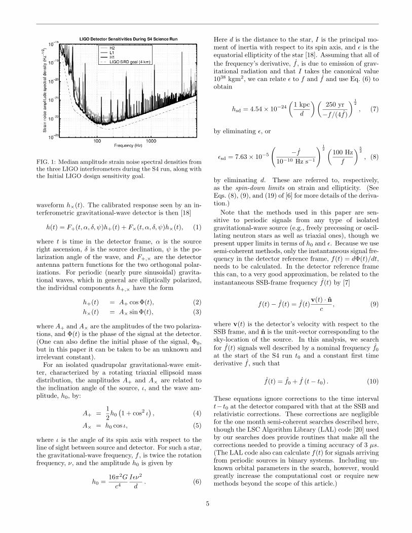
FIG. 1: Median amplitude strain noise spectral densities fromthe three LIGO interferometers during the S4 run, along withthe Initial LIGO design sensitivity goal.
waveform h×(t). The calibrated response seen by an in-terferometric gravitational-wave detector is then [18]
h(t) = F+(t, α, δ, ψ)h+(t) + F×(t, α, δ, ψ)h×(t), (1)
where t is time in the detector frame, α is the sourceright ascension, δ is the source declination, ψ is the po-larization angle of the wave, and F+,× are the detectorantenna pattern functions for the two orthogonal polar-izations. For periodic (nearly pure sinusoidal) gravita-tional waves, which in general are elliptically polarized,the individual components h+,× have the form
h+(t) = A+ cos Φ(t), (2)h×(t) = A× sin Φ(t), (3)
where A+ and A× are the amplitudes of the two polariza-tions, and Φ(t) is the phase of the signal at the detector.(One can also define the initial phase of the signal, Φ0,but in this paper it can be taken to be an unknown andirrelevant constant).
For an isolated quadrupolar gravitational-wave emit-ter, characterized by a rotating triaxial ellipsoid massdistribution, the amplitudes A+ and A× are related tothe inclination angle of the source, ι, and the wave am-plitude, h0, by:
A+ =12h0
(1 + cos2 ι
), (4)
A× = h0 cos ι, (5)
where ι is the angle of its spin axis with respect to theline of sight between source and detector. For such a star,the gravitational-wave frequency, f , is twice the rotationfrequency, ν, and the amplitude h0 is given by
h0 =16π2G
c4Iεν2
d. (6)
Here d is the distance to the star, I is the principal mo-ment of inertia with respect to its spin axis, and ε is theequatorial ellipticity of the star [18]. Assuming that all ofthe frequency’s derivative, f , is due to emission of grav-itational radiation and that I takes the canonical value1038 kgm2, we can relate ε to f and f and use Eq. (6) toobtain
hsd = 4.54× 10⁻²⁴
(1 kpcd
)(250 yr−f/(4f)
) 12
, (7)
by eliminating ε, or
εsd = 7.63× 10⁻⁵
(−f
10−10 Hz s−1
) 12 (100 Hz
f
) 52
, (8)
by eliminating d. These are referred to, respectively,as the spin-down limits on strain and ellipticity. (SeeEqs. (8), (9), and (19) of [6] for more details of the deriva-tion.)
Note that the methods used in this paper are sen-sitive to periodic signals from any type of isolatedgravitational-wave source (e.g., freely precessing or oscil-lating neutron stars as well as triaxial ones), though wepresent upper limits in terms of h0 and ε. Because we usesemi-coherent methods, only the instantaneous signal fre-quency in the detector reference frame, f(t) = dΦ(t)/dt,needs to be calculated. In the detector reference framethis can, to a very good approximation, be related to theinstantaneous SSB-frame frequency f(t) by [7]
f(t)− f(t) = f(t)v(t) · n
c, (9)
where v(t) is the detector’s velocity with respect to theSSB frame, and n is the unit-vector corresponding to thesky-location of the source. In this analysis, we searchfor f(t) signals well described by a nominal frequency f0at the start of the S4 run t0 and a constant first timederivative f , such that
f(t) = f0 + f (t− t0) . (10)
These equations ignore corrections to the time intervalt− t0 at the detector compared with that at the SSB andrelativistic corrections. These corrections are negligiblefor the one month semi-coherent searches described here,though the LSC Algorithm Library (LAL) code [20] usedby our searches does provide routines that make all thecorrections needed to provide a timing accuracy of 3 µs.(The LAL code also can calculate f(t) for signals arrivingfrom periodic sources in binary systems. Including un-known orbital parameters in the search, however, wouldgreatly increase the computational cost or require newmethods beyond the scope of this article.)
5
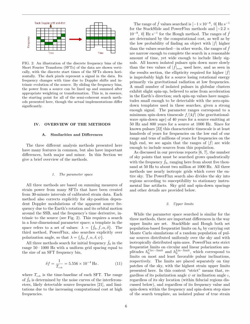
FIG. 2: An illustration of the discrete frequency bins of theShort Fourier Transform (SFTs) of the data are shown verti-cally, with the discrete start times of the SFTs shown hori-zontally. The dark pixels represent a signal in the data. Itsfrequency changes with time due to Doppler shifts and in-trinsic evolution of the source. By sliding the frequency bins,the power from a source can be lined up and summed afterappropriate weighting or transformation. This is, in essence,the starting point for all of the semi-coherent search meth-ods presented here, though the actual implementations differsignificantly.
IV. OVERVIEW OF THE METHODS
A. Similarities and Differences
The three different analysis methods presented herehave many features in common, but also have importantdifferences, both major and minor. In this Section wegive a brief overview of the methods.
1. The parameter space
All three methods are based on summing measures ofstrain power from many SFTs that have been createdfrom 30-minute intervals of calibrated strain data. Eachmethod also corrects explicitly for sky-position depen-dent Doppler modulations of the apparent source fre-quency due to the Earth’s rotation and its orbital motionaround the SSB, and the frequency’s time derivative, in-trinsic to the source (see Fig. 2). This requires a searchin a four-dimensional parameter space; a template in thespace refers to a set of values: λ = f0, f , α, δ. Thethird method, PowerFlux, also searches explicitly overpolarization angle, so that λ = f0, f , α, δ, ψ.
All three methods search for initial frequency f0 in therange 50 – 1000 Hz with a uniform grid spacing equal tothe size of an SFT frequency bin,
δf =1Tcoh
= 5.556× 10⁻⁴ Hz . (11)
where Tcoh is the time-baseline of each SFT. The rangeof f0 is determined by the noise curves of the interferom-eters, likely detectable source frequencies [21], and limi-tations due to the increasing computational cost at highfrequencies.
The range of f values searched is [−1×10⁻⁸, 0] Hz s−1
for the StackSlide and PowerFlux methods and [−2.2 ×10⁻⁹, 0] Hz s−1 for the Hough method. The ranges of fare determined by the computational cost, as well as bythe low probability of finding an object with |f | higherthan the values searched—in other words, the ranges of fare narrow enough to complete the search in a reasonableamount of time, yet wide enough to include likely sig-nals. All known isolated pulsars spin down more slowlythan the two values of |f |max used here, and as seen inthe results section, the ellipticity required for higher |f |is improbably high for a source losing rotational energyprimarily via gravitational radiation at low frequencies.A small number of isolated pulsars in globular clustersexhibit slight spin-up, believed to arise from accelerationin the Earth’s direction; such spin-up values have magni-tudes small enough to be detectable with the zero-spin-down templates used in these searches, given a strongenough signal. The parameter ranges correspond to aminimum spin-down timescale f/|4f | (the gravitational-wave spin-down age) of 40 years for a source emitting at50 Hz and 800 years for a source at 1000 Hz. Since forknown pulsars [22] this characteristic timescale is at leasthundreds of years for frequencies on the low end of ourrange and tens of millions of years for frequencies on thehigh end, we see again that the ranges of |f | are wideenough to include sources from this population.
As discussed in our previous reports [6, 7], the numberof sky points that must be searched grows quadraticallywith the frequency f0, ranging here from about five thou-sand at 50 Hz to about two million at 1000 Hz. All threemethods use nearly isotropic grids which cover the en-tire sky. The PowerFlux search also divides the sky intoregions according to susceptibility to stationary instru-mental line artifacts. Sky grid and spin-down spacingsand other details are provided below.
2. Upper limits
While the parameter space searched is similar for thethree methods, there are important differences in the wayupper limits are set. StackSlide and Hough both setpopulation-based frequentist limits on h0 by carrying outMonte Carlo simulations of a random population of pul-sar sources distributed uniformly over the sky and withisotropically distributed spin-axes. PowerFlux sets strictfrequentist limits on circular and linear polarization am-plitudes hCirc−limit
0 and hLin−limit0 , which correspond to
limits on most and least favorable pulsar inclinations,respectively. The limits are placed separately on tinypatches of the sky, with the highest strain upper limitspresented here. In this context “strict” means that, re-gardless of its polarization angle ψ or inclination angle ι,regardless of its sky location (within fiducial regions dis-cussed below), and regardless of its frequency value andspin-down within the frequency and spin-down step sizesof the search template, an isolated pulsar of true strain
6
amplitude h0 = 2hLin−limit0 , would have yielded a higher
measured amplitude than what we measure, in at least95% of independent observations. The circular polariza-tion limits hCirc−limit
0 apply only to the most favorableinclinations (ι ≈ 0, π), regardless of sky location andregardless of frequency and spin-down, as above.
Due to these different upper limit setting methods,sharp instrumental lines are also handled differently.StackSlide and Hough carry out removal of known instru-mental lines of varying widths in individual SFTs. Themeasured powers in those bins are replaced with randomnoise generated to mimic the noise observed in neigh-boring bins. This line cleaning technique can lead to atrue signal being missed because its apparent frequencymay coincide with an instrumental line for a large num-ber of SFTs. However, population-averaged upper limitsare determined self-consistently to include loss of detec-tion efficiency due to line removal, by using Monte Carlosimulations.
Since its limits are intended to be strict, that is, validfor any source inclination and for any source locationwithin its fiducial area, PowerFlux must handle instru-mental lines differently. Single-bin lines are flagged dur-ing data preparation so that when searching for a partic-ular source an individual SFT bin power is ignored whenit coincides with the source’s apparent frequency. If morethan 80% of otherwise eligible bins are excluded for thisreason, no attempt is made to set a limit on strain powerfrom that source. In practice, however, the 80% cutoff isnot used because we have found that all such sources liein certain unfavorable regions of the sky, which we call“skybands” and which we exclude when setting upperlimits. These skybands depend on source frequency andits derivative, as described in Sec. V D 4.
3. Data Preparation
Other differences among the methods concern the datawindowing and filtering used in computing Fourier trans-forms and concern the noise estimation. StackSlide andHough apply high pass filters to the data above 40Hz, inaddition to the filter used to produce the calibrated datastream, and use Tukey windowing. PowerFlux applies noadditional filtering and uses Hann windowing with 50%overlap between adjacent SFT’s. StackSlide and Houghuse median-based noise floor tracking [23, 24, 25]. Incontrast, Powerflux uses a time-frequency decomposition.Both of these noise estimation methods are described inSec. V.
The raw, uncalibrated data channels containing thestrain measurements from the three interferometers areconverted to a calibrated “h(t)” data stream, followingthe procedure described in [26], using calibration refer-ence functions described in [27]. SFTs are generated di-rectly from the calibrated data stream, using 30-minuteintervals of data for which the interferometer is operat-ing in what is known as science-mode. The choice of 30
minutes is a tradeoff between intrinsic sensitivity, whichincreases with SFT length, and robustness against fre-quency drift during the SFT interval due to the Earth’smotion, source spin-down, and non-stationarity of thedata [7]. The requirement that each SFT contain contigu-ous data at nominal sensitivity introduces duty factor lossfrom edge effects, especially for the Livingston interfer-ometer ('20%) which had typically shorter contiguous-data stretches. In the end, the StackSlide and Houghsearches used 1004 SFTs from H1 and 899 from L1,the two interferometers with the best broadband sen-sitivty. For PowerFlux, the corresponding numbers ofoverlapped SFTs were 1925 and 1628. The Hough searchalso used 1063 H2 SFTs. In each case, modest require-ments were placed on data quality to avoid short periodswith known electronic saturations, unmonitored calibra-tion strengths, and the periods immediately precedingloss of optical cavity resonance.
B. Definitions And Notation
Let N be the number of SFTs, Tcoh the time-baselineof each SFT, and M the number of uniformly spaceddata points in the time domain from which the SFT isconstructed. If the time series is denoted by xj (j =0, 1, 2 . . .M − 1), then our convention for the discreteFourier transform is
xk = ∆tM−1∑j=0
xje−2πijk/M , (12)
where k = 0, 1, 2 . . . (M − 1), and ∆t = Tcoh/M . For0 ≤ k ≤ M/2, the frequency index k corresponds to aphysical frequency of fk = k/Tcoh.
In each method, the “power” (in units of spectral den-sity) associated with frequency bin k and SFT i is takento be
P ik =2|xik|2
Tcoh
. (13)
It proves convenient to define a normalized power by
ρik =P ikSik
. (14)
The quantity Sik is the single-sided power spectral densityof the detector noise at frequency fk, the estimation ofwhich is described below. Furthermore, a threshold, ρth,can be used to define a binary count by [10]:
nik =
1 if ρik ≥ ρth
0 if ρik < ρth. (15)
When searching for a signal using template λ the de-tector antenna pattern and frequency of the signal arefound at the midpoint time of the data used to gener-ate each SFT. Frequency dependent quantities are then
7

Quantity Description
Pi Power for SFT i & template λ
ρi Normalized power for SFT i & template λ
ni Binary count for SFT i & template λ
Si Power spect. noise density for SFT i & template λ
F i+ F+ at midpoint of SFT i for template λ
F i× F× at midpoint of SFT i for template λ
TABLE I: Summary of notation used.
evaluated at a frequency index k corresponding to the binnearest this frequency. To simplify the equations in therest of this paper we drop the frequency index k and usethe notation given in Table I to define various quantitiesfor SFT i and template λ.
C. Basic StackSlide, Hough, and PowerFluxFormalism
We call the detection statistics used in this search the“StackSlide Power”, P , the “Hough Number Count”, n,and the “PowerFlux Signal Estimator”, R. The basicdefinitions of these quantities are given below.
Here the simple StackSlide method described in [15]is used; the “StackSlide Power” for a given template isdefined as
P =1N
N−1∑i=0
ρi , (16)
This normalization results in values of P with a meanvalue of unity and, for Gaussian noise, a standard devi-ation of 1/
√N . Details about the value and statistics of
P in the presence and absence of a signal are given inAppendix B and [15].
In the Hough search, instead of summing the normal-ized power, the final statistic used in this paper is aweighted sum of the binary counts, giving the “HoughNumber Count”:
n =N−1∑i=0
wini . (17)
where the Hough weights are defined as
wi ∝1Si
(F i+)2
+(F i×)2
, (18)
and the weight normalization is chosen according to
N−1∑i=0
wi = N . (19)
With this choice of normalization the Hough NumberCount n lies within the range [0, N ]. Thus, we take a
binary count ni to have greater weight if the SFT i has alower noise floor and if, in the time-interval correspond-ing to this SFT, the beam pattern functions are largerfor a particular point in the sky. Note that the sensitiv-ity of the search is governed by the ratios of the differentweights, not by the choice of overall scale. In the next sec-tion we show that these weights maximize the sensitivity,averaged over the orientation of the source. This choiceof wi was originally derived in [16] using a different argu-ment and is similar to that used in the PowerFlux circularpolarization projection described next. More about theHough method is given in [7, 10].
The PowerFlux method takes advantage of the factthat less weight should be given to times of greater noisevariance or smaller detector antenna response to a signal.Noting that power estimated from the data divided bythe antenna pattern increases the variance of the data attimes of small detector response, the problem reduces tofinding weights that minimize the variance, or in otherwords that maximize the signal-to-noise ratio. The re-sulting PowerFlux detection statistic is [17],
R =2Tcoh
∑N−1i=0 WiPi/(F
iψ)2∑N−1
i=0 Wi
, (20)
where the PowerFlux weights are defined as
Wi = [(F iψ)2]2/S2i , (21)
and where
(F iψ)2 =
(F i+)2 linear polarization
(F i+)2 + (F i×)2 circular polarization. (22)
As noted previously, the PowerFlux method searches us-ing four linear polarization projections and one circularpolarization projection. For the linear polarization pro-jections, note that (F i+)2 is evaluated at the angle ψ,which is the same as (F i×)2 evaluated at the angle ψ−π/4;for circular polarization, the value of (F i+)2 +(F i×)2 is in-dependent of ψ. Finally note that the factor of 2/Tcoh inEq. (20) makes R dimensionless and is chosen to make itdirectly related to an estimate of the squared amplitudeof the signal for the given polarization. Thus R is alsocalled in this paper the “PowerFlux Signal Estimator”.(See [17] and Appendix A for further discussion.)
We have shown in Eqs. (16)-(22) how to compute thedetection statistic (or signal estimator) for a given tem-plate. The next section gives the details of the imple-mentation and pipelines used, where these quantities arecalculated for a set of templates λ and analyzed.
V. IMPLEMENTATIONS AND PIPELINES
A. Running Median Noise Estimation
The implementations of the StackSlide and Houghmethods described below use a “running median” to esti-mate the mean power and, from this estimate, the power
8
spectral density of the noise, for every frequency bin ofevery SFT. PowerFlux uses a different noise decomposi-tion method described in its implementation section be-low.
Note that for Gaussian noise, the single-sided powerspectral density can be estimated using
Sik∼=
2〈|xik|2〉Tcoh
(23)
where the angle brackets represent an ensemble average.The estimation of Sik must guard against any biases in-troduced by the presence of a possible signal and alsoagainst narrow spectral disturbances. For this reason themean, 〈|xik|2〉, is estimated via the median. We assumethat the noise is stationary within a single SFT, but al-low for non-stationarities across different SFTs. In everySFT we calculate the “running median” of |xik|2 for ev-ery 101 frequency bins centered on the kth bin, and thenestimate 〈|xik|2〉 [23, 24, 25] by dividing by the expectedratio of the median to the mean.
Note, however, that in the StackSlide search, afterthe estimated mean power is used to compute Sik inthe denominator of Eq. (14) these terms are summed inEq. (16), while the Hough search applies a cutoff to ob-tain binary counts in Eq. (15) before summing. This re-sults in the use of a different correction to get the meanin the StackSlide search from that used in the Houghsearch. For a running median using 101 frequency bins,the effective ratio of the median to mean used in theStackSlide search was 0.691162 (which was chosen to nor-malize the data so that the mean value of the StackSlidePower equals one) compared with the expected ratio foran exponential distribution of 0.698073 used in the Houghsearch (which is explained in Appendix A of [7]). It is im-portant to realize that the results reported here are validindependent of the factor used, since any overall constantscaling of the data does not affect the selection of outliersor the reported upper limits, which are based on MonteCarlo injections subjected to the same normalization.
B. The StackSlide Implementation
1. Algorithm and parameter space
The StackSlide method uses power averaging to gainsensitivity by decreasing the variance of the noise [12, 13,14, 15]. Brady and Creighton [12] first described this ap-proach in the context of gravitational-wave detection asa part of a hierarchical search for periodic sources. Theirmethod consists of averaging the power from a demodu-lated time series, but as an approximation did not includethe beam pattern response of the detector. In Ref. [15],a simple implementation is described that averages thenormalized power given in Eq. (14). Its extension to aver-aging the maximum likelihood statistic (known as the F-statistic) which does include the beam pattern response
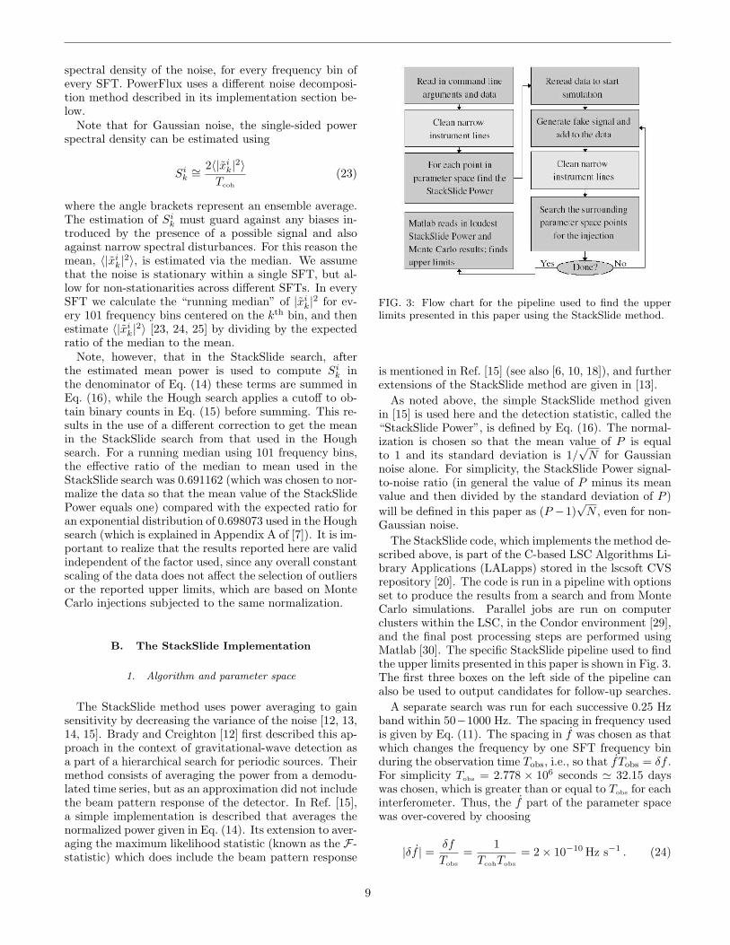
FIG. 3: Flow chart for the pipeline used to find the upperlimits presented in this paper using the StackSlide method.
is mentioned in Ref. [15] (see also [6, 10, 18]), and furtherextensions of the StackSlide method are given in [13].
As noted above, the simple StackSlide method givenin [15] is used here and the detection statistic, called the“StackSlide Power”, is defined by Eq. (16). The normal-ization is chosen so that the mean value of P is equalto 1 and its standard deviation is 1/
√N for Gaussian
noise alone. For simplicity, the StackSlide Power signal-to-noise ratio (in general the value of P minus its meanvalue and then divided by the standard deviation of P )will be defined in this paper as (P −1)
√N , even for non-
Gaussian noise.The StackSlide code, which implements the method de-
scribed above, is part of the C-based LSC Algorithms Li-brary Applications (LALapps) stored in the lscsoft CVSrepository [20]. The code is run in a pipeline with optionsset to produce the results from a search and from MonteCarlo simulations. Parallel jobs are run on computerclusters within the LSC, in the Condor environment [29],and the final post processing steps are performed usingMatlab [30]. The specific StackSlide pipeline used to findthe upper limits presented in this paper is shown in Fig. 3.The first three boxes on the left side of the pipeline canalso be used to output candidates for follow-up searches.
A separate search was run for each successive 0.25 Hzband within 50−1000 Hz. The spacing in frequency usedis given by Eq. (11). The spacing in f was chosen as thatwhich changes the frequency by one SFT frequency binduring the observation time Tobs, i.e., so that fTobs = δf .For simplicity Tobs = 2.778 × 10⁶ seconds ' 32.15 dayswas chosen, which is greater than or equal to Tobs for eachinterferometer. Thus, the f part of the parameter spacewas over-covered by choosing
|δf | = δf
Tobs
=1
TcohTobs
= 2× 10⁻¹⁰ Hz s−1 . (24)
9
Values of f in the range [−1 × 10⁻⁸ Hz s−1, 0 Hz s−1]were searched. This range corresponds to a search over51 values of f , which is the same as PowerFlux used inits low-frequency search (discussed in Section. V D).
The sky grid used is similar to that used for the all-sky search in [6], but with a spacing between sky-gridpoints appropriate for the StackSlide search. This grid isisotropic on the celestial sphere, with an angular spacingbetween points chosen for the 50-225 Hz band, such thatthe maximum change in Doppler shift from one sky gridpoint to the next would shift the frequency by half a bin.This is given by
δθ0 =0.5 c δf
f(v sinθ)max
= 9.3× 10⁻³ rad(
300Hz
f
), (25)
where v is the magnitude of the velocity v of the detectorin the SSB frame, and θ is the angle between v and theunit-vector n giving the sky-position of the source. Equa-tions (24) and (25) are the same as Eqs. (19) and (22) in[7], which represent conservative choices that over-coverthe parameter space. Thus, the parameter space usedhere corresponds to that in Ref. [7], adjusted to the S4observation time, and with the exception that a stere-ographic projection of the sky is not used. Rather anisotropic sky grid is used like the one used in [6].
One difficulty is that the computational cost of thesearch increases quadratically with frequency, due to theincreasing number of points on the sky grid. To reducethe computational time, the sky grid spacing given inEq. (25) was increased by a factor of 5 above 225 Hz.This represents a savings of a factor of 25 in computa-tional cost. It was shown through a series of simulations,comparing the upper limits in various frequency bandswith and without the factor of 5 increase in grid spacing,that this changes the upper limits on average by less thanthan 0.3%, with a standard deviation of 2%. Thus, thisfactor of 5 increase was used to allow the searches in the225− 1000 Hz band to complete in a reasonable amountof time.
It is not surprising that the sky grid spacing can be in-creased, for at least three reasons. First, the value for δθ0given in Eq. (25) applies to only a small annular region onthe sky, and is smaller than the average change. Second,only the net change in Doppler shift during the observa-tion time is important, which is less than the maximumDoppler shift due to the Earth’s orbital motion duringa one month run. (If the Doppler shift were constantduring the entire observation time, one would not needto search sky positions even if the Doppler shift variedacross the sky. A source frequency would be shifted bya constant amount during the observation, and would bedetected, albeit in a frequency bin different from thatat the SSB.) Third, because of correlations on the sky,one can detect a signal with negligible loss of SNR muchfarther from its sky location than the spacing above sug-gests.
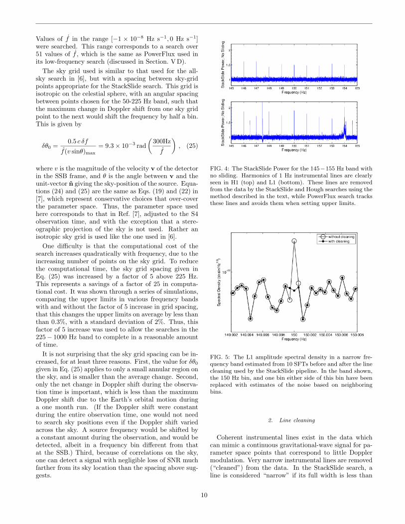
FIG. 4: The StackSlide Power for the 145−155 Hz band withno sliding. Harmonics of 1 Hz instrumental lines are clearlyseen in H1 (top) and L1 (bottom). These lines are removedfrom the data by the StackSlide and Hough searches using themethod described in the text, while PowerFlux search tracksthese lines and avoids them when setting upper limits.
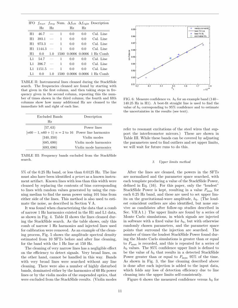
FIG. 5: The L1 amplitude spectral density in a narrow fre-quency band estimated from 10 SFTs before and after the linecleaning used by the StackSlide pipeline. In the band shown,the 150 Hz bin, and one bin either side of this bin have beenreplaced with estimates of the noise based on neighboringbins.
2. Line cleaning
Coherent instrumental lines exist in the data whichcan mimic a continuous gravitational-wave signal for pa-rameter space points that correspond to little Dopplermodulation. Very narrow instrumental lines are removed(“cleaned”) from the data. In the StackSlide search, aline is considered “narrow” if its full width is less than
10
IFO fstart fstep Num. ∆fleft ∆fright Description
Hz Hz Hz Hz
H1 46.7 — 1 0.0 0.0 Cal. Line
H1 393.1 — 1 0.0 0.0 Cal. Line
H1 973.3 — 1 0.0 0.0 Cal. Line
H1 1144.3 — 1 0.0 0.0 Cal. Line
H1 0.0 1.0 1500 0.0006 0.0006 1 Hz Comb
L1 54.7 — 1 0.0 0.0 Cal. Line
L1 396.7 — 1 0.0 0.0 Cal. Line
L1 1151.5 — 1 0.0 0.0 Cal. Line
L1 0.0 1.0 1500 0.0006 0.0006 1 Hz Comb
TABLE II: Instrumental lines cleaned during the StackSlidesearch. The frequencies cleaned are found by starting withthat given in the first column, and then taking steps in fre-quency given in the second column, repeating this the num-ber of times shown in the third column; the fourth and fifthcolumns show how many additional Hz are cleaned to theimmediate left and right of each line.
Excluded Bands Description
Hz
[57, 63) Power lines
[n60− 1, n60 + 1) n = 2 to 16 Power line harmonics
[340, 350) Violin modes
[685, 690) Violin mode harmonics
[693, 696) Violin mode harmonics
TABLE III: Frequency bands excluded from the StackSlidesearch.
5% of the 0.25 Hz band, or less than 0.0125 Hz. The linemust also have been identified a priori as a known instru-ment artifact. Known lines with less than this width werecleaned by replacing the contents of bins correspondingto lines with random values generated by using the run-ning median to find the mean power using 101 bins fromeither side of the lines. This method is also used to esti-mate the noise, as described in Section V A.
It was found when characterizing the data that a combof narrow 1 Hz harmonics existed in the H1 and L1 data,as shown in Fig. 4. Table II shows the lines cleaned dur-ing the StackSlide search. As the table shows, only thiscomb of narrow 1 Hz harmonics and injected lines usedfor calibration were removed. As an example of the clean-ing process, Fig. 5 shows the amplitude spectral densityestimated from 10 SFTs before and after line cleaning,for the band with the 1 Hz line at 150 Hz.
The cleaning of very narrow lines has a negligible effecton the efficiency to detect signals. Very broad lines, onthe other hand, cannot be handled in this way. Bandswith very broad lines were searched without any linecleaning. There were also a number of highly disturbedbands, dominated either by the harmonics of 60 Hz powerlines or by the violin modes of the suspended optics, thatwere excluded from the StackSlide results. (Violin modes
FIG. 6: Measure confidence vs. h0 for an example band (140−140.25 Hz in H1). A best-fit straight line is used to find thevalue of h0 corresponding to 95% confidence and to estimatethe uncertainties in the results (see text).
refer to resonant excitations of the steel wires that sup-port the interferometer mirrors.) These are shown inTable III. While these bands can be covered by adjustingthe parameters used to find outliers and set upper limits,we will wait for future runs to do this.
3. Upper limits method
After the lines are cleaned, the powers in the SFTsare normalized and the parameter space searched, witheach template producing a value of the StackSlide Power,defined in Eq. (16). For this paper, only the “loudest”StackSlide Power is kept, resulting in a value Pmax foreach 0.25 Hz band, and these are used to set upper lim-its on the gravitational-wave amplitude, h0. (The loud-est coincident outliers are also identified, but none sur-vive as candidates after follow-up studies described inSec. VII A 1.) The upper limits are found by a series ofMonte Carlo simulations, in which signals are injectedin software with a fixed value for h0, but with otherwiserandomly chosen parameters, and the parameter spacepoints that surround the injection are searched. Thenumber of times the loudest StackSlide Power found dur-ing the Monte Carlo simulations is greater than or equalto Pmax is recorded, and this is repeated for a series ofh0 values. The 95% confidence upper limit is defined tobe the value of h0 that results in a detected StackSlidePower greater than or equal to Pmax 95% of the time.As shown in Fig. 3, the line cleaning described aboveis done after each injection is added to the input data,which folds any loss of detection efficiency due to linecleaning into the upper limits self-consistently.
Figure 6 shows the measured confidence versus h0 for
11

an example frequency band. The upper limit finding pro-cess involves first making an initial guess of its value, thenrefining this guess using a single set of injections to findan estimate of the upper limit, and finally using this es-timate to run several sets of injections to find the finalvalue of the upper limit. These steps are now describedin detail.
To start the upper limit finding process, first an initialguess, hguess
0 , is used as the gravitational-wave amplitude.The initial guess need not be near the sought-after upperlimit, just sufficiently large, as explained below. A singleset of n injections is done (specifically n = 3000 was used)with random sky positions and isotropically distributedspin axes, but all with amplitude hguess
0 . The outputlist of StackSlide Powers from this set of injections issorted in ascending order and the 0.05n’th (specificallyfor n = 3000 the 150th) smallest value of the StackSlidePower is found, which we call P0.05, Note that the goal isto find the value of h0 that makes P0.05 = Pmax, so that95% of the output powers are greater than the maximumpower found during the search. This is what we call the95% confidence upper limit. Of course, in general P0.05
will not equal Pmax unless our first guess was very lucky.However, as per the discussion concerning Eq. (B5), P−1is proportional to h2
0 (i.e, removing the mean value dueto noise leaves on average the power due to the presenceof a signal). Thus, an estimate of the 95% h0 confidenceupper limits is given by the following rescaling of hguess
0 ,
hest0 =
√Pmax − 1√P0.05 − 1
hguess0 . (26)
Thus an estimated upper limit, hest0 , is found from a sin-
gle set of injections with amplitude hguess0 ; the only re-
quirement is that hguess0 is chosen loud enough to make
P0.05 > 1.It is found that using Eq. (26) results in a estimate of
the upper limit that is typically within 10% of the finalvalue. For example, the estimated upper limit found inthis way is indicated by the circled point in Fig. 6. Thevalue of hest
0 then becomes the first value for h0 in a seriesof Monte Carlo simulations, each with 3000 injections,which use this value and 8 neighboring values, measur-ing the confidence each time. The Matlab [30] polyfitand polyval functions are then used to find the best-fitstraight line to determine the value of h0 correspondingto 95% confidence and to estimate the uncertainties inthe results. This is the final step of the pipeline shownin Fig. 3.
C. The Hough Transform Implementation
1. Description of Algorithm
The Hough transform is a general method for patternrecognition, invented originally to analyze bubble cham-ber pictures from CERN [31, 32]; it has found many
applications in the analysis of digital images [33]. Thismethod has already been used to analyze data from thesecond science run (S2) of the LIGO detectors [7] and adetailed description can be found in [10]. Here we presentonly a brief description, emphasizing the differences be-tween the previous S2 search and the S4 search describedhere.
The Hough search uses a weighted sum of the binarycounts as its final statistic, as given by Eqs. (15) and (19).In the standard Hough search as presented in [7, 10], theweights are all set to unity. The weighted Hough trans-form was originally discussed in [16]. The software forperforming the Hough transform has been adapted to usearbitrary weights without any significant loss in compu-tational efficiency. Furthermore, the robustness of theHough transform method in the presence of strong tran-sient disturbances is not compromised by using weightsbecause each SFT contributes at most wi (which is oforder unity) to the final number count.
The following statements can be proven using themethods of [10]. The mean number count in the ab-sence of a signal is n = Np, where N is the numberof SFTs and p is the probability that the normalizedpower, of a given frequency bin and SFT defined byEq. (14), exceeds a threshold ρth, i.e., p is the proba-bility that a frequency bin is selected in the absence ofa signal. For unity weighting, the standard deviation issimply σ =
√Np(1− p). However, with more general
weighting, it can be shown that σ is given by
σ =√||w||2p(1− p) , (27)
where ||w||2 =∑N−1i=0 w2
i . A threshold nth on the numbercount corresponding to a false alarm rate αH is given by
nth = Np+√
2||w||2p(1− p) erfc−1(2αH) . (28)
Therefore nth depends on the weights of the correspond-ing template λ. In this case, the natural detection statis-tic is not the “Hough Number Count” n, but the signifi-cance of a number count, defined by
s =n− nσ
, (29)
where n and σ are the expected mean and standard de-viation for pure noise. Values of s can be compared di-rectly across different templates characterized by differ-ing weight distributions.
The threshold ρth (c.f. Eq. 15) is selected to give theminimum false dismissal probability βH for a given falsealarm rate. In [7] it was shown that the optimal choice forρth is 1.6 which correspond to a peak selection probabilityp = e−ρth ≈ 0.2. It can be shown that the optimal choiceis unchanged by the weights and hence ρth = 1.6 is usedonce more [34].
Consider a population of sources located at a givenpoint in the sky, but having uniformly distributed spinaxis directions. For a template that is perfectly matched
12
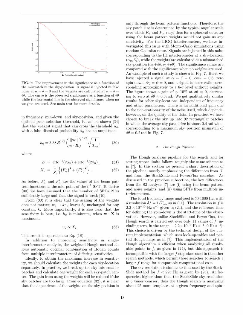
FIG. 7: The improvement in the significance as a function ofthe mismatch in the sky-position. A signal is injected in fakenoise at α = δ = 0 and the weights are calculated at α = δ =δθ. The curve is the observed significance as a function of δθwhile the horizontal line is the observed significance when noweights are used. See main text for more details.
in frequency, spin-down, and sky-position, and given theoptimal peak selection threshold, it can be shown [34]that the weakest signal that can cross the threshold nth
with a false dismissal probability βH has an amplitude
h0 = 3.38 S1/2
(||w||w ·X
)1/2√ 1Tcoh
, (30)
where
S = erfc−1(2αH) + erfc−1(2βH) , (31)
Xi =1Si
(F i+)2
+(F i×)2
. (32)
As before, F i+ and F i× are the values of the beam pat-tern functions at the mid-point of the ith SFT. To derive(30) we have assumed that the number of SFTs N issufficiently large and that the signal is weak [10].
From (30) it is clear that the scaling of the weightsdoes not matter; wi → kwi leaves h0 unchanged for anyconstant k. More importantly, it is also clear that thesensitivity is best, i.e. h0 is minimum, when w · X ismaximum:
wi ∝ Xi . (33)
This result is equivalent to Eq. (18).In addition to improving sensitivity in single-
interferometer analysis, the weighted Hough method al-lows automatic optimal combination of Hough countsfrom multiple interferometers of differing senstivities.
Ideally, to obtain the maximum increase in sensitiv-ity, we should calculate the weights for each sky-locationseparately. In practice, we break up the sky into smallerpatches and calculate one weight for each sky-patch cen-ter. The gain from using the weights will be reduced if thesky patches are too large. From equation (32), it is clearthat the dependence of the weights on the sky-position is
only through the beam pattern functions. Therefore, thesky patch size is determined by the typical angular scaleover which F+ and F× vary; thus for a spherical detectorusing the beam pattern weights would not gain us anysensitivity. For the LIGO interferometers, we have in-vestigated this issue with Monte-Carlo simulations usingrandom Gaussian noise. Signals are injected in this noisecorresponding to the H1 interferometer at a sky-location(α0, δ0), while the weights are calculated at a mismatchedsky-position (α0+δθ, δ0+δθ). The significance values arecompared with the significance when no weights are used.An example of such a study is shown in Fig. 7. Here, wehave injected a signal at α = δ = 0, cos ι = 0.5, zerospin-down, Φ0 = ψ = 0, and a signal to noise ratio corre-sponding approximately to a 6-σ level without weights.The figure shows a gain of ∼ 10% at δθ = 0, decreas-ing to zero at δθ ≈ 0.3 rad. We get qualitatively similarresults for other sky-locations, independent of frequencyand other parameters. There is an additional gain dueto the non-stationarity of the noise itself, which depends,however, on the quality of the data. In practice, we havechosen to break the sky up into 92 rectangular patchesin which the average sky patch size is about 0.4 rad wide,corresponding to a maximum sky position mismatch ofδθ = 0.2 rad in Fig. 7.
2. The Hough Pipeline
The Hough analysis pipeline for the search and forsetting upper limits follows roughly the same scheme asin [7]. In this section we present a short description ofthe pipeline, mostly emphasizing the differences from [7]and from the StackSlide and PowerFlux searches. Asdiscussed in the previous subsection, the key differencesfrom the S2 analysis [7] are (i) using the beam-patternand noise weights, and (ii) using SFTs from multiple in-terferometers.
The total frequency range analyzed is 50-1000 Hz, witha resolution δf = 1/Tcoh as in (11). The resolution in f is2.2× 10−10 Hz s−1 given in (24), and the reference timefor defining the spin-down is the start-time of the obser-vation. However, unlike StackSlide and PowerFlux, theHough search is carried out over only 11 values of f , in-cluding zero, in the range [−2.2×10⁻⁹ Hz s−1, 0 Hz s−1].This choice is driven by the technical design of the cur-rent implementation, which uses look-up-tables and par-tial Hough maps as in [7]. This implementation of theHough algorithm is efficient when analyzing all resolv-able points in f , as given in (24), but this approach isincompatible with the larger f step sizes used in the othersearch methods, which permit those searches to search alarger f range for comparable computational cost.
The sky resolution is similar to that used by the Stack-Slide method for f < 225 Hz as given by (25). At fre-quencies higher than this, the StackSlide sky-resolutionis 5 times coarser, thus the Hough search is analyzingabout 25 more templates at a given frequency and spin-
13

FIG. 8: Two example histograms of the normalized Houghnumber count compared to a Gaussian distribution for the H1detector in the frequency band 150-151 Hz. The upper figurecorresponds to a a patch located at the north pole for thecase in which the weights are used. The number of templatesanalyzed in this 1Hz band is of 11× 106, the number of SFTs1004, the corresponding mean n = 202.7 and σ = 12.94 isobtained from the weights. The lower figure corresponds toa patch at the equator using the same data. In this case thenumber of templates analyzed in this 1Hz band is of 10.5×10⁶,and its corresponding σ = 14.96.
down value. In each of the 92 sky patches, by means ofthe stereographic projection, the sky patch is mapped toa two dimensional plane with a uniform grid of that res-olution δθ0. Sky Patches slightly overlap to avoid gapsamong them (see [7] for further details).
Figure 8 shows examples of histograms of the numbercounts in two particular sky patches for the H1 detectorin the 150-151 Hz band. In all the bands free of instru-mental disturbances, the Hough number count distribu-tions follows the expected theoretical distribution, whichcan be approximated by a Gaussian distribution. Sincethe number of SFTs for H1 is 1004, the corresponding
IFO fstart fstep n ∆fleft ∆fright Description
Hz Hz Hz Hz
H1 392.365 — 1 0.01 0.01 Cal. SideBand
H1 393.835 — 1 0.01 0.01 Cal. SideBand
H2 54.1 — 1 0.0 0.0 Cal. Line
H2 407.3 — 1 0.0 0.0 Cal. Line
H2 1159.7 — 1 0.0 0.0 Cal. Line
H2 110.934 36.9787 4 0.02 0.02 37 Hz Oscillator
L1 154.6328 8.1386 110 0.01 0.01 8.14 Hz Comb
L1 0.0 36.8725 50 0.02 0.02 37 Hz Oscillator (*)
TABLE IV: Instrumental lines cleaned during the Houghsearch that were not listed in Table II (see text). (*) Theselines were removed only in the multi-interferometer search.
mean n = 202.7 and the standard deviation is given byEq. (27). The standard deviation is computed from theweights w and varies among different sky patches becauseof varying antenna pattern functions.
The upper limits on h0 are derived from the loud-est event, registered over the entire sky and spin-downrange in each 0.25 Hz band, not from the highest numbercount. As for the StackSlide method, we use a frequentistmethod, where upper limits refer to a hypothetical pop-ulation of isolated spinning neutron stars which are uni-formly distributed in the sky and have a spin-down ratef uniformly distributed in the range [−2.2×10⁻⁹ Hz s−1,0 Hz s−1]. We also assume uniform distributions for theparameters cos ι ∈ [−1, 1], ψ ∈ [0, 2π], and Φ0 ∈ [0, 2π].The strategy for calculating the 95% upper limits isroughly the same scheme as in [7], except for the treat-ment of narrow instrumental lines.
Known spectral disturbances are removed from theSFTs in the same way as for the StackSlide search. Theknown spectral lines are, of course, also consistently re-moved after each signal injection when performing theMonte-Carlo simulations to obtain the upper limits.
The narrow instrumental lines “cleaned” from the SFTdata are the same ones cleaned during the StackSlidesearch shown in Table II, together with ones listed in Ta-ble IV. The additional lines listed in Table IV are cleanedto prevent large artifacts in one instrument from increas-ing the false alarm rate of the Hough multi-interferometersearch. Note that the L1 36.8725 Hz comb was eliminatedmid-way through the S4 run by replacing a synthesizedradio frequency oscillator for phase modulation with acrystal oscillator, and these lines were not removed inthe Hough L1 single-interferometer analysis.
No frequency bands have been excluded from theHough search, although the upper limits reported on thebands shown in Table III, that are dominated by 60 Hzpower line harmonics or violin modes of the suspendedoptics, did not always give satisfactory convergence to anupper limit. In a few of these very noisy bands, upperlimits were set by extrapolation, instead of interpolation,of the Monte-Carlo simulations. Therefore the results
14
!
!
"
#
"$ $
%&'$
FIG. 9: Flow chart for the pipeline used to find the upperlimits presented in this paper using the PowerFlux method.
reported on those bands have larger error bars. No pa-rameter tuning was performed on these disturbed bandsto improve the upper limits.
D. The Powerflux Implementation
The PowerFlux method is a variant on the StackSlidemethod in which the contributions from each SFT areweighted by the inverse square of the average spectralpower density in each band and weighted according tothe antenna pattern sensitivity of the interferometer foreach point searched on the sky. This weighting schemehas two advantages: 1) variance on the signal strengthestimator is minimized, improving signal-to-noise ratio;and 2) the estimator is itself a direct measure of sourcestrain power, allowing direct parameter estimation anddramatically reducing dependence on Monte Carlo sim-ulations. Details of software usage and algorithms canbe found in a technical document [17]. Figure 9 shows aflow chart of the algorithm, discussed in detail below.
1. Noise decomposition
Noise estimation is carried out through atime/frequency noise decomposition procedure inwhich the dominant variations are factorized within each
nominal 0.25 Hz band as a product of a spectral variationand a time variation across the data run. Specifically,for each 0.25 Hz band, a matrix of logarithms of powermeasurements across the 0.56 mHz SFT bins and acrossthe SFT’s of the run is created. Two vectors, denotedTMedians and FMedians, are initially set to zero andthen iteratively updated according to the followingalgorithm:
1. For each SFT (row in matrix), the median value(logarithm of power) is computed and then addedto the corresponding element of TMedians whilesubtracted from each matrix element in that row.
2. For each frequency bin (column in matrix), the me-dian value is computed and then added to the corre-sponding FMedians element, while subtracted fromeach matrix element in that column.
3. The procedure repeats from step 1 until all medianscomputed in steps 1 and 2 are zero (or negligible).
The above algorithm typically converges quickly. Thesize of the frequency band treated increases with centralfrequency, as neighboring bins are included to allow formaximum and minimum Doppler shifts to be searched inthe next step.
For stationary, Gaussian noise and for noise that fol-lows the above assumptions of underlying factorized fre-quency and time dependence, the expected distributionof residual matrix values can be found from simulation.Figure 10 shows a sample expected residual power distri-bution following noise decomposition for simulated sta-tionary, Gaussian data, along with a sample residualpower distribution from the S4 data (0.25-Hz band of H1near 575 Hz, in this case) following noise decomposition.The agreement in shape between these two distributionsis very good and is typical of the S4 data, despite some-times large variations in the corresponding TMedians andFMedians vectors, and despite, in this case, the presenceof a moderately strong simulated pulsar signal (Pulsar2in Table V).
The residuals are examined for outliers. If the largestresidual value is found to lie above a threshold of 1.5,that corresponding 0.25 Hz band is flagged as containinga “wandering line” because a strong but drifting instru-mental line can lead to such outliers. The value 1.5 isdetermined empirically from Gaussian simulations. Anextremely strong pulsar could also be flagged in this way,and indeed the strongest injected pulsars are labelled aswandering lines. Hence in the search, the wandering linesare followed up, but no upper limits are quoted here forthe affected bands.
2. Line flagging
Sharp instrumental lines can prevent accurate noise es-timation for pulsars that have detected frequencies in thesame 0.56 mHz bin as the line. In addition, strong lines
15

FIG. 10: Typical residual logarithmic power following noisedecomposition for a sample 0.25-Hz band of H1 data (crosses)near 575 Hz in a band containing an injected pulsar. Theresidual is defined as the difference between a measured powerfor a given frequency bin in a given 30-minute period and thevalue predicted by the FMedians and TMedians vectors. Thesmooth curve is for a simulation in Gaussian noise.
tend to degrade achievable sensitivity by adding excessapparent power in an affected search. In early LIGO sci-ence runs, including the S4 run, there have been sharpinstrumental lines at multiples of 1 Hz or 0.25 Hz, arisingfrom artifacts in the data acquisition electronics.
To mitigate the most severe of these effects, the Pow-erFlux algorithm performs a simple line detection andflagging algorithm. For each 0.25 Hz band, the detectedsummed powers are ranked and an estimated Gaussiansigma computed from the difference in the 50% and 94%quantiles. Any bins with power greater than 5.0 σ aremarked for ignoring in subsequent processing. Specifi-cally, when carrying out a search for a pulsar of a nomi-nal true frequency, its contribution to the signal estima-tor is ignored when the detected frequency would lie inthe same 0.56 mHz bin as a detected line. As discussedbelow, for certain frequencies, spin-downs and points inthe sky, the fraction of time a putative pulsar has a de-tected frequency in a bin containing an instrumental linecan be quite large, requiring care. The deliberate ignor-ing of contributing bins affected by sharp instrumentallines does not lead to a bias in resulting limits, but itdoes degrade sensitivity, from loss of data. In any 0.25Hz band, no more than five bins may be flagged as lines.Any band with more than five line candidates is exam-ined manually.
3. Signal estimator
Once the noise decomposition is complete, with esti-mates of the spectral noise density for each SFT, the
PowerFlux algorithm computes a weighted sum of thestrain powers, where the weighting takes into accountthe underlying time and spectral variation contained inTMedians and FMedians and the antenna pattern sensi-tivity for an assumed sky location and incident wave po-larization. Specifically, for an assumed polarization angleψ and sky location, the following quantity is defined foreach bin k of each SFT i:
Qi =Pi
(F iψ)2, (34)
where F iψ is the ψ-dependent antenna pattern for the skylocation, defined in Eq. (22). (See also Appendix A.)
As in Sec. IV B, to simplify the notation we defineQi = Pi/(F
iψ)2 as the value of Qi for SFT i and a given
template λ.For each individual SFT bin power measurement Pi,
one expects an underlying exponential distribution, witha standard deviation equal to the mean, a statement thatholds too for Qi. To minimize the variance of a signalestimator based on a sum of these powers, each contribu-tion is weighted by the inverse of the expected variance ofthe contribution. Specifically, we compute the followingsignal estimator:
R =2Tcoh
(∑i
1(Qi)2
)−1∑i
Qi(Qi)2
, (35)
=2Tcoh
(∑i
[(F iψ)2]2
(Pi)2
)−1∑i
(F iψ)2Pi(Pi)2
, (36)
where Pi and Qi are the expected uncorrected andantenna-corrected powers of SFT i averaged over fre-quency. Since the antenna factor is constant in this av-erage, Qi = Pi/(F
iψ)2. Furthermore, Pi is a estimate of
the power spectral density of the noise. The replacementPi∼= Si gives Eq. (20).Note that for an SFT i with low antenna pattern sen-
sitivity |F iψ|, the signal estimator receives a small con-tribution. Similarly, SFT’s i for which ambient noiseis high receive small contributions. Because computa-tional time in the search grows linearly with the numberof SFT’s and because of large time variations in noise,it proves efficient to ignore SFT’s with sky-dependentand polarization-dependent effective noise higher than acutoff value. The cutoff procedure saves significant com-puting time, with negligible effect on search performance.
Specifically, the cutoff is computed as follows. Let σjbe the ordered estimated standard deviations in noise,taken to be the ordered means of Qi = 1
kmaxΣkQik, where
kmax is the number of frequency bins used in the searchtemplate. Define jopt to be the index jmax for which
the quantity 1jmax
√Σjmaxj=1 σ
2j is minimized. Only SFT’s
for which σj < 2σjopt are used for signal estimation. Inwords, jopt defines the last SFT that improves ratherthan degrades signal estimator variance in an unweighted
16

FIG. 11: Sky map of run-summed PowerFlux weights for a0.25-Hz band near 575 Hz for one choice of linear polarizationin the S4 H1 data. The normalization corresponds roughly tothe effective number of median-noise SFT’s contributing tothe sum.
mean. For the weighted mean used here, the effectivenoise contributions are allowed to be as high as twice thevalue found for jopt. The choice of 2σjopt is determinedempirically.
The PowerFlux search sets strict, frequentist, all-sky95% confidence-level upper limits on the flux of gravita-tional radiation bathing the Earth. To be conservative inthe strict limits, numerical corrections to the signal esti-mator are applied: 1) a factor of 1/ cos(π/8) = 1.082 formaximum linear polarization mismatch, based on twicethe maximum half-angle of mismatch (see Appendix A)and 2) a factor of 1.22 for bin-centered signal power lossdue to Hann windowing (applied during SFT generation);and 3) a factor of 1.19 for drift of detected signal fre-quency across the width of the 0.56 mHz bins used inthe SFT’s. Note that the use of rectangular windowingwould eliminate the need for correction 2) above, butwould require a larger correction of 1.57 for 3)
Antenna pattern and noise weighting in the PowerFluxmethod allows weaker sources to be detected in certainregions of the sky, where run-averaged antenna patternsdiscriminate in declination and diurnal noise variationsdiscriminate in right ascension. Figure 11 illustrates theresulting variation in effective noise across the sky for a0.25-Hz H1 band near 575 Hz for the circular polariza-tion projection. By separately examining SNR, one mayhope to detect a signal in a sensitive region of the skywith a strain significantly lower than suggested by thestrict worst-case all-sky frequentist limits presented here,as discussed below in section VI D. Searches are carriedout for four linear polarizations, ranging over polariza-tion angle from ψ = 0 to ψ = 3
8π in steps of π/8 and for(unique) circular polarization.
A useful computational savings comes from definingtwo different sky resolutions. A “coarse” sky gridding isused for setting the cutoff value defined above, while finegrid points are used for both frequency and amplitudedemodulation. A typical ratio of number of coarse gridpoints to number of fine grid points used for Dopplercorrections is 25.
4. Sky banding
Stationary and near-stationary instrumental spectrallines can be mistaken for a periodic source of gravita-tional radiation if the nominal source parameters are con-sistent with small variation in detected frequency duringthe time of observation. The variation in the frequencyat the detector can be found by taking the time derivativeof Eq. (9), which gives,
df
dt=(
1 +v(t) · n
c
)f + f(t)
a(t) · nc
. (37)
The detector’s acceleration, a in this equation is domi-nated by the Earth’s orbital acceleration aEarth, since thediurnal part of the detector’s acceleration is small andapproximately averages to zero during the observation.Thus, it should be emphasized that a single instrumentalline can mimic sources with a range of slightly differentfrequencies and assumed different positions in the skythat lie in an annular band. For a source f assumed tobe zero, the center of the band is defined by a circle 90degrees away from the direction of the average acceler-ation of the Earth during the run where aEarth · n = 0,i.e., toward the average direction of the Sun during therun. For source spin-downs different from zero, there canbe a cancellation between assumed spin-down (or spinup)that is largely cancelled by the Earth’s average accelera-tion, leading to a shift of the annular region of apparentDoppler stationarity toward (away from) the Sun.
A figure of merit found to be useful for discriminatingregions of “good” sky from “bad” sky (apparent detectedfrequency is highly stationary) is the “S parameter”:
S = f + [(Ω× vEarth/c) · n)]f0, (38)
where Ω is the Earth’s angular velocity vector about thesolar system barycenter. The term Ω× vEarth is a mea-sure of the Earth’s average acceleration during the run,where vEarth is taken to be the noise-weighted velocityof the H1 detector during the run. Regions of sky withsmall |S| for a given f and f have stationary detectedfrequency. As discussed below in section VI D, such re-gions are not only prone to high false-alarm rates, butthe line flagging procedure described in section V D 2leads to systematically underestimated signal strengthand invalid upper limits. Hence limits are presented herefor only sources with |S| greater than a threshold valuedenoted Slarge. The minimum acceptable value chosenfor Slarge is found from software signal injections to be1.1 × 10−9 Hz s−1 for the 1-month S4 run and can beunderstood to be
Slarge =Noccupied bins
Tobs · Tcoh, (39)
where Noccupied bins ∼ 5 is the minimum total num-ber of 0.56 mHz detection bins occupied by the source
17

FIG. 12: S4 sky band regions (good - light gray, bad for L1- medium or dark gray, bad for H1 & L1 - dark gray) for a
source frequency f = 100 Hz and three different assumed spin-down choices: a) zero; b) −3×10⁻⁹ Hz s−1; and c) −1×10⁻⁸
Hz s−1. The black circle indicates the average position of theSun during the data run.
during the data run for reliable detection. In prac-tice, we use still larger values for the H1 interferome-ter (Slarge = 1.85 × 10⁻⁹ Hz s−1) and L1 interferom-eter (Slarge = 3.08 × 10⁻⁹ Hz s−1) during the S4 runfor the limits presented here because of a pervasive andstrong comb of precise 1-Hz lines in both interferometers.These lines, caused by a GPS-second synchronized elec-tronic disturbance and worse in L1 than in H1, lead tohigh false-alarm rates from that data for lower values ofSlarge. For the frequency and spin-down ranges searchedin this analysis, the average fractions of sky lost to theskyband veto are 15% for H1 and 26% for L1.
Figures 12-14 illustrate the variation in the fraction ofsky marked as “bad” as assumed source frequency andspin-down are varied. Generally, at low frequencies, largesky regions are affected, but only for low spin-down mag-nitude, while at high frequencies, small sky regions areaffected, but the effects are appreciable to larger spin-down magnitude. It should be noted that the annularregions of the sky affected depend upon the start timeand duration of a data run. The longer the data run, thesmaller is the region of sky for which Doppler stationar-ity is small. Future LIGO data runs of longer durationshould have only small regions near the ecliptic poles forwhich stationary instrumental lines prove troublesome.
FIG. 13: S4 sky band regions (good - light gray, bad for L1- medium or dark gray, bad for H1 & L1 - dark gray) for a
source frequency f = 300 Hz and three different assumed spin-down choices: a) zero; b) −3×10⁻⁹ Hz s−1; and c) −1×10⁻⁸
Hz s−1. The black circle indicates the average position of theSun during the data run.
5. Grid-point upper limit determination
An intermediate step in the PowerFlux analysis is thesetting of upper limits on signal strength for each sky-point for each 0.56 mHz bin. The limits presented herefor each interferometer are the highest of these interme-diate limits for each 0.25-Hz band over the entire “good”sky. The intermediate limits are set under the assump-tion of Gaussian residuals in noise. In brief, for each0.56 mHz bin and sky-point, a Feldman-Cousins [35]95% confidence-level is set for an assumed normal dis-tribution with a standard deviation determined robustlyfrom quantiles of the entire 0.25 Hz band. The Feldman-Cousins approach provides the virtues of a well behavedupper limit even when background noise fluctuates wellbelow its expectation value and of smooth transition be-tween 1-sided and 2-sided limits, but in practice the high-est upper limit for any 0.25 Hz band is invariably thehighest measured power plus 1.96 times the estimatedstandard deviation on the background power for that bin,corresponding to a conventional a priori 1-sided 97.5%upper CL. A Kolmogorov-Smirnov (KS) statistic is com-puted to check the actual power against a Gaussian dis-tribution for each 0.25 Hz band. Those bands that fail theKS test value of 0.07 (> 5σ deviation for the S4 data sam-ple) are flagged as “Non-Gaussian”, and no upper limits
18
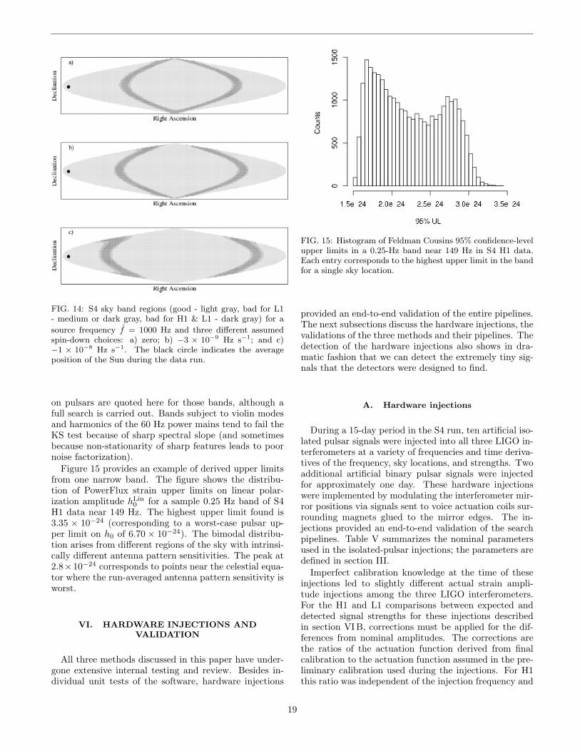
FIG. 14: S4 sky band regions (good - light gray, bad for L1- medium or dark gray, bad for H1 & L1 - dark gray) for a
source frequency f = 1000 Hz and three different assumedspin-down choices: a) zero; b) −3 × 10⁻⁹ Hz s−1; and c)−1 × 10⁻⁸ Hz s−1. The black circle indicates the averageposition of the Sun during the data run.
on pulsars are quoted here for those bands, although afull search is carried out. Bands subject to violin modesand harmonics of the 60 Hz power mains tend to fail theKS test because of sharp spectral slope (and sometimesbecause non-stationarity of sharp features leads to poornoise factorization).
Figure 15 provides an example of derived upper limitsfrom one narrow band. The figure shows the distribu-tion of PowerFlux strain upper limits on linear polar-ization amplitude hLin
0 for a sample 0.25 Hz band of S4H1 data near 149 Hz. The highest upper limit found is3.35 × 10−24 (corresponding to a worst-case pulsar up-per limit on h0 of 6.70 × 10⁻²⁴). The bimodal distribu-tion arises from different regions of the sky with intrinsi-cally different antenna pattern sensitivities. The peak at2.8×10−24 corresponds to points near the celestial equa-tor where the run-averaged antenna pattern sensitivity isworst.
VI. HARDWARE INJECTIONS ANDVALIDATION
All three methods discussed in this paper have under-gone extensive internal testing and review. Besides in-dividual unit tests of the software, hardware injections
FIG. 15: Histogram of Feldman Cousins 95% confidence-levelupper limits in a 0.25-Hz band near 149 Hz in S4 H1 data.Each entry corresponds to the highest upper limit in the bandfor a single sky location.
provided an end-to-end validation of the entire pipelines.The next subsections discuss the hardware injections, thevalidations of the three methods and their pipelines. Thedetection of the hardware injections also shows in dra-matic fashion that we can detect the extremely tiny sig-nals that the detectors were designed to find.
A. Hardware injections
During a 15-day period in the S4 run, ten artificial iso-lated pulsar signals were injected into all three LIGO in-terferometers at a variety of frequencies and time deriva-tives of the frequency, sky locations, and strengths. Twoadditional artificial binary pulsar signals were injectedfor approximately one day. These hardware injectionswere implemented by modulating the interferometer mir-ror positions via signals sent to voice actuation coils sur-rounding magnets glued to the mirror edges. The in-jections provided an end-to-end validation of the searchpipelines. Table V summarizes the nominal parametersused in the isolated-pulsar injections; the parameters aredefined in section III.
Imperfect calibration knowledge at the time of theseinjections led to slightly different actual strain ampli-tude injections among the three LIGO interferometers.For the H1 and L1 comparisons between expected anddetected signal strengths for these injections describedin section VI B, corrections must be applied for the dif-ferences from nominal amplitudes. The corrections arethe ratios of the actuation function derived from finalcalibration to the actuation function assumed in the pre-liminary calibration used during the injections. For H1this ratio was independent of the injection frequency and
19
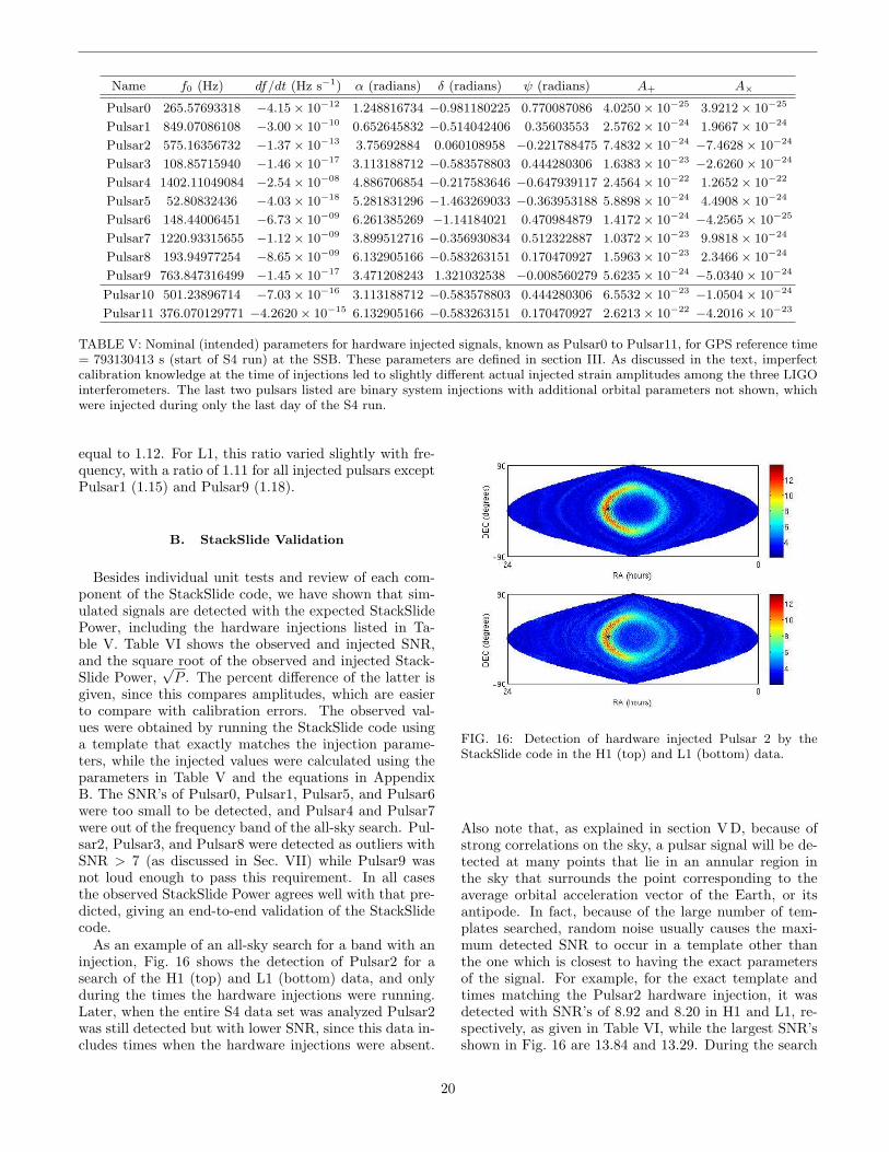
Name f0 (Hz) df/dt (Hz s−1) α (radians) δ (radians) ψ (radians) A+ A×
Pulsar0 265.57693318 −4.15× 10⁻¹² 1.248816734 −0.981180225 0.770087086 4.0250× 10⁻²⁵ 3.9212× 10⁻²⁵
Pulsar1 849.07086108 −3.00× 10⁻¹⁰ 0.652645832 −0.514042406 0.35603553 2.5762× 10⁻²⁴ 1.9667× 10⁻²⁴
Pulsar2 575.16356732 −1.37× 10⁻¹³ 3.75692884 0.060108958 −0.221788475 7.4832× 10⁻²⁴ −7.4628× 10⁻²⁴
Pulsar3 108.85715940 −1.46× 10⁻¹⁷ 3.113188712 −0.583578803 0.444280306 1.6383× 10⁻²³ −2.6260× 10⁻²⁴
Pulsar4 1402.11049084 −2.54× 10−08 4.886706854 −0.217583646 −0.647939117 2.4564× 10⁻²² 1.2652× 10⁻²²
Pulsar5 52.80832436 −4.03× 10⁻¹⁸ 5.281831296 −1.463269033 −0.363953188 5.8898× 10⁻²⁴ 4.4908× 10⁻²⁴
Pulsar6 148.44006451 −6.73× 10−09 6.261385269 −1.14184021 0.470984879 1.4172× 10⁻²⁴ −4.2565× 10⁻²⁵
Pulsar7 1220.93315655 −1.12× 10−09 3.899512716 −0.356930834 0.512322887 1.0372× 10⁻²³ 9.9818× 10⁻²⁴
Pulsar8 193.94977254 −8.65× 10−09 6.132905166 −0.583263151 0.170470927 1.5963× 10⁻²³ 2.3466× 10⁻²⁴
Pulsar9 763.847316499 −1.45× 10⁻¹⁷ 3.471208243 1.321032538 −0.008560279 5.6235× 10⁻²⁴ −5.0340× 10⁻²⁴
Pulsar10 501.23896714 −7.03× 10⁻¹⁶ 3.113188712 −0.583578803 0.444280306 6.5532× 10⁻²³ −1.0504× 10⁻²⁴
Pulsar11 376.070129771 −4.2620× 10⁻¹⁵ 6.132905166 −0.583263151 0.170470927 2.6213× 10⁻²² −4.2016× 10⁻²³
TABLE V: Nominal (intended) parameters for hardware injected signals, known as Pulsar0 to Pulsar11, for GPS reference time= 793130413 s (start of S4 run) at the SSB. These parameters are defined in section III. As discussed in the text, imperfectcalibration knowledge at the time of injections led to slightly different actual injected strain amplitudes among the three LIGOinterferometers. The last two pulsars listed are binary system injections with additional orbital parameters not shown, whichwere injected during only the last day of the S4 run.
equal to 1.12. For L1, this ratio varied slightly with fre-quency, with a ratio of 1.11 for all injected pulsars exceptPulsar1 (1.15) and Pulsar9 (1.18).
B. StackSlide Validation
Besides individual unit tests and review of each com-ponent of the StackSlide code, we have shown that sim-ulated signals are detected with the expected StackSlidePower, including the hardware injections listed in Ta-ble V. Table VI shows the observed and injected SNR,and the square root of the observed and injected Stack-Slide Power,
√P . The percent difference of the latter is
given, since this compares amplitudes, which are easierto compare with calibration errors. The observed val-ues were obtained by running the StackSlide code usinga template that exactly matches the injection parame-ters, while the injected values were calculated using theparameters in Table V and the equations in AppendixB. The SNR’s of Pulsar0, Pulsar1, Pulsar5, and Pulsar6were too small to be detected, and Pulsar4 and Pulsar7were out of the frequency band of the all-sky search. Pul-sar2, Pulsar3, and Pulsar8 were detected as outliers withSNR > 7 (as discussed in Sec. VII) while Pulsar9 wasnot loud enough to pass this requirement. In all casesthe observed StackSlide Power agrees well with that pre-dicted, giving an end-to-end validation of the StackSlidecode.
As an example of an all-sky search for a band with aninjection, Fig. 16 shows the detection of Pulsar2 for asearch of the H1 (top) and L1 (bottom) data, and onlyduring the times the hardware injections were running.Later, when the entire S4 data set was analyzed Pulsar2was still detected but with lower SNR, since this data in-cludes times when the hardware injections were absent.
FIG. 16: Detection of hardware injected Pulsar 2 by theStackSlide code in the H1 (top) and L1 (bottom) data.
Also note that, as explained in section V D, because ofstrong correlations on the sky, a pulsar signal will be de-tected at many points that lie in an annular region inthe sky that surrounds the point corresponding to theaverage orbital acceleration vector of the Earth, or itsantipode. In fact, because of the large number of tem-plates searched, random noise usually causes the maxi-mum detected SNR to occur in a template other thanthe one which is closest to having the exact parametersof the signal. For example, for the exact template andtimes matching the Pulsar2 hardware injection, it wasdetected with SNR’s of 8.92 and 8.20 in H1 and L1, re-spectively, as given in Table VI, while the largest SNR’sshown in Fig. 16 are 13.84 and 13.29. During the search
20
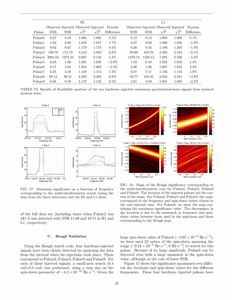
H1 L1
Observed Injected Observed Injected Percent Observed Injected Observed Injected Percent
Pulsar SNR SNR√P
√P Difference SNR SNR
√P
√P Difference
Pulsar0 0.27 0.23 1.006 1.005 0.1% 0.15 0.13 1.003 1.003 0.1%
Pulsar1 1.62 0.80 1.035 1.017 1.7% 0.27 0.69 1.006 1.016 −1.0%
Pulsar2 8.92 8.67 1.179 1.175 0.4% 8.20 9.34 1.180 1.203 −1.9%
Pulsar3 199.78 174.72 3.124 2.943 6.2% 89.89 104.76 2.304 2.454 −6.1%
Pulsar4 2081.64 1872.24 9.607 9.116 5.4% 1279.12 1425.14 7.895 8.326 −5.2%
Pulsar5 0.05 1.30 1.001 1.028 −2.6% 1.02 0.44 1.024 1.010 1.4%
Pulsar6 0.17 2.94 1.004 1.063 −5.5% 2.90 1.36 1.067 1.032 3.4%
Pulsar7 6.25 5.50 1.129 1.114 1.3% 6.07 5.11 1.136 1.116 1.8%
Pulsar8 98.12 96.21 2.303 2.285 0.8% 92.77 103.45 2.334 2.441 −4.4%
Pulsar9 6.68 6.59 1.137 1.135 0.2% 2.61 3.69 1.061 1.085 −2.2%
TABLE VI: Results of StackSlide analyses of the ten hardware injected continuous gravitational-wave signals from isolatedneutron stars.
FIG. 17: Maximum significance as a function of frequencycorresponding to the multi-interferometer search (using thedata from the three detectors) and the H1 and L1 alone.
of the full data set (including times when Pulsar2 wasoff) it was detected with SNR 11.09 and 10.71 in H1 andL1, respectively.
C. Hough Validation
Using the Hough search code, four hardware-injectedsignals have been clearly detected by analyzing the datafrom the interval when the injections took place. Thesecorrespond to Pulsar2, Pulsar3, Pulsar8 and Pulsar9. Foreach of these injected signals, a small-area search (0.4rad×0.4 rad) was performed, using a step size on thespin-down parameter of −4.2× 10⁻¹⁰ Hz s−1. Given the
FIG. 18: Maps of the Hough significance corresponding tothe multi-interferometer case for Pulsar2, Pulsar3, Pulsar8and Pulsar9. The location of the injected pulsars are the cen-ters of the maps. For Pulsar2, Pulsar3 and Pulsar9, the mapscorrespond to the frequency and spin-down values closest tothe real injected ones. For Pulsar8, we show the map con-taining the maximum significance value. The discrepancy insky location is due to the mismatch in frequency and spin-down values between those used in the injections and thosecorresponding to the Hough map.
large spin-down value of Pulsar8 (−8.65× 10⁻⁹ Hz s−1),we have used 23 values of the spin-down spanning therange [−9.24× 10⁻⁹ Hz s−1, 0 Hz s−1] to search for thispulsar. Because of its large amplitude, Pulsar8 can bedetected even with a large mismatch in the spin-downvalue, although at the cost of lower SNR.
Figure 17 shows the significance maximized over differ-ent sky locations and spin-down values for the differentfrequencies. These four hardware injected pulsars have
21
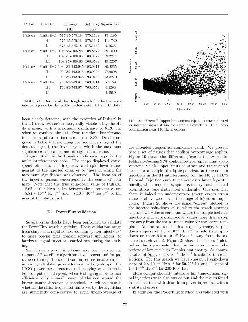
Pulsar Detector f0 range f0(max) Significance
(Hz) (Hz)
Pulsar2 Multi-IFO 575.15-575.18 575.1689 15.1195
H1 575.15-575.18 575.1667 11.1730
L1 575.15-575.18 575.1650 9.7635
Pulsar3 Multi-IFO 108.855-108.86 108.8572 39.1000
H1 108.855-108.86 108.8572 32.2274
L1 108.855-108.86 108.8589 19.2267
Pulsar8 Multi-IFO 193.932-193.945 193.9411 39.2865
H1 193.932-193.945 193.9394 27.9008
L1 193.932-193.945 193.9400 23.8270
Pulsar9 Multi-IFO 763.83-763.87 763.8511 8.3159
H1 763.83-763.87 763.8556 6.1268
L1 - - 5.4559
TABLE VII: Results of the Hough search for the hardwareinjected signals for the multi-interferometer, H1 and L1 data.
been clearly detected, with the exception of Pulsar9 inthe L1 data. Pulsar9 is marginally visible using the H1data alone, with a maximum significance of 6.13, butwhen we combine the data from the three interferome-ters, the significance increases up to 8.32. Details aregiven in Table VII, including the frequency range of thedetected signal, the frequency at which the maximumsignificance is obtained and its significance value.
Figure 18 shows the Hough significance maps for themulti-interferometer case. The maps displayed corre-spond either to the frequency and spin-down valuesnearest to the injected ones, or to those in which themaximum significance was observed. The location ofthe injected pulsars correspond to the center of eachmap. Note that the true spin-down value of Pulsar8,−8.65× 10⁻⁹ Hz s−1, lies between the parameter values−8.82 × 10⁻⁹ Hz s−1 and −8.40 × 10⁻⁹ Hz s−1 of thenearest templates used.
D. PowerFlux validation
Several cross checks have been performed to validatethe PowerFlux search algorithm. These validations rangefrom simple and rapid Fourier-domain “power injections”to more precise time domain software simulations, tohardware signal injections carried out during data tak-ing.
Signal strain power injections have been carried outas part of PowerFlux algorithm development and for pa-rameter tuning. These software injections involve super-imposing calculated powers for assumed signals upon theLIGO power measurements and carrying out searches.For computational speed, when testing signal detectionefficiency, only a small region of the sky around theknown source direction is searched. A critical issue iswhether the strict frequentist limits set by the algorithmare sufficiently conservative to avoid undercoverage of
FIG. 19: “Excess” (upper limit minus injected) strain plottedvs injected signal strain for sample PowerFlux H1 elliptic-polarization near 140 Hz injections.
the intended frequentist confidence band. We presenthere a set of figures that confirm overcoverage applies.Figure 19 shows the difference (“excess”) between theFeldman-Cousins 95% confidence-level upper limit (con-ventional 97.5% upper limit) on strain and the injectedstrain for a sample of elliptic-polarization time-domaininjections in the H1 interferometer for the 140.50-140.75Hz band. Injection amplitudes were distributed logarith-mically, while frequencies, spin-downs, sky locations, andorientations were distributed uniformly. One sees thatthere is indeed no undercoverage (every excess strainvalue is above zero) over the range of injection ampli-tudes. Figure 20 shows the same “excess” plotted vsthe injected spin-down value, where the search assumesa spin-down value of zero, and where the sample includesinjections with actual spin-down values more than a stepsize away from the the assumed value for the search tem-plate. As one can see, in this frequency range, a spin-down stepsize of 1.0 × 10⁻⁹ Hz s−1 is safe (true spin-down no more 5.0 × 10⁻¹⁰ Hz s−1 away from the as-sumed search value). Figure 21 shows the “excess” plot-ted vs the S parameter that discriminates between skyregions of low and high Doppler stationarity. As shown,a value of Slarge ∼ 1 × 10⁻⁹ Hz s−1 is safe for these in-jections. For this search we have chosen 51 spin-downsteps of 2 × 10⁻¹⁰ Hz s−1 for 50-225 Hz and 11 steps of1× 10−9 Hz s−1 for 200-1000 Hz.
More computationally intensive full time-domain sig-nal injections were also carried out and the results foundto be consistent with those from power injections, withinstatistical errors.
In addition, the PowerFlux method was validated with
22
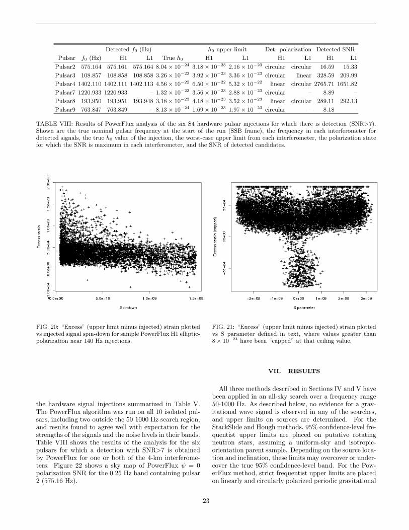
Detected f0 (Hz) h0 upper limit Det. polarization Detected SNR
Pulsar f0 (Hz) H1 L1 True h0 H1 L1 H1 L1 H1 L1
Pulsar2 575.164 575.161 575.164 8.04× 10⁻²⁴ 3.18× 10⁻²³ 2.16× 10⁻²³ circular circular 16.59 15.33
Pulsar3 108.857 108.858 108.858 3.26× 10⁻²³ 3.92× 10⁻²³ 3.36× 10⁻²³ circular linear 328.59 209.99
Pulsar4 1402.110 1402.111 1402.113 4.56× 10⁻²² 6.50× 10⁻²² 5.32× 10⁻²² linear circular 2765.71 1651.82
Pulsar7 1220.933 1220.933 – 1.32× 10⁻²³ 3.56× 10⁻²³ 2.88× 10⁻²³ circular – 8.89 –
Pulsar8 193.950 193.951 193.948 3.18× 10⁻²³ 4.18× 10⁻²³ 3.52× 10⁻²³ linear circular 289.11 292.13
Pulsar9 763.847 763.849 – 8.13× 10⁻²⁴ 1.69× 10⁻²³ 1.97× 10⁻²³ circular – 8.18 –
TABLE VIII: Results of PowerFlux analysis of the six S4 hardware pulsar injections for which there is detection (SNR>7).Shown are the true nominal pulsar frequency at the start of the run (SSB frame), the frequency in each interferometer fordetected signals, the true h0 value of the injection, the worst-case upper limit from each interferometer, the polarization statefor which the SNR is maximum in each interferometer, and the SNR of detected candidates.
FIG. 20: “Excess” (upper limit minus injected) strain plottedvs injected signal spin-down for sample PowerFlux H1 elliptic-polarization near 140 Hz injections.
the hardware signal injections summarized in Table V.The PowerFlux algorithm was run on all 10 isolated pul-sars, including two outside the 50-1000 Hz search region,and results found to agree well with expectation for thestrengths of the signals and the noise levels in their bands.Table VIII shows the results of the analysis for the sixpulsars for which a detection with SNR>7 is obtainedby PowerFlux for one or both of the 4-km interferome-ters. Figure 22 shows a sky map of PowerFlux ψ = 0polarization SNR for the 0.25 Hz band containing pulsar2 (575.16 Hz).
FIG. 21: “Excess” (upper limit minus injected) strain plottedvs S parameter defined in text, where values greater than8× 10−24 have been “capped” at that ceiling value.
VII. RESULTS
All three methods described in Sections IV and V havebeen applied in an all-sky search over a frequency range50-1000 Hz. As described below, no evidence for a grav-itational wave signal is observed in any of the searches,and upper limits on sources are determined. For theStackSlide and Hough methods, 95% confidence-level fre-quentist upper limits are placed on putative rotatingneutron stars, assuming a uniform-sky and isotropic-orientation parent sample. Depending on the source loca-tion and inclination, these limits may overcover or under-cover the true 95% confidence-level band. For the Pow-erFlux method, strict frequentist upper limits are placedon linearly and circularly polarized periodic gravitational
23

FIG. 22: Sample sky map of Feldman Cousins upper limitson circularly polarized strain for a 0.25-Hz band containinghardware-injected Pulsar 2 at 575.16 Hz. Only the data (halfthe run) during which the pulsar injection was enabled hasbeen analyzed for this plot. The injected pulsar (h0 = 8.0 ×10⁻²⁴) stands out clearly above background. (Right ascensionincreases positively toward the left and declination toward thetop of the sky map.)
FIG. 23: The loudest observed StackSlide Power for H1 (top)and L1 (bottom). Frequency bands with the harmonics of 60Hz and the violin modes have been removed.
wave sources, assuming worst-case sky location, avoidingundercoverage. The limits on linear polarization are alsore-interpreted as limits on rotating neutron stars, assum-ing worst-case sky location and worst-case star inclina-tion. The following subsections describe these results indetail.
A. StackSlide Results
1. Loudest powers and coincidence outliers
The StackSlide method was applied to the S4 H1 andL1 data set, as given in Sec. V B. As described in thatsection, only the loudest StackSlide Power was returnedfrom a search of the entire sky, the range of the fre-quency’s time derivative, [−1 × 10⁻⁸, 0] Hz s−1, and for
FIG. 24: The loudest observed StackSlide Power for H1 (top)and L1 (bottom) with a simple veto applied: only outliersin each 0.25 Hz band with SNR > 7 in both interferometersthat have a fractional frequency difference ≤ 2.2 × 10⁻⁴ arekept. These are shown against the background results thathave SNR ≤ 7 in both interferometers. Frequency bands withthe harmonics of the 60 Hz and the violin modes have alsobeen removed.
fH1 (Hz) fL1 (Hz) H1 SNR L1 SNR Comment
1 78.618889 78.618889 14.82 13.58 Inst. Lines
2 108.856111 108.856111 152.11 69.79 HW Inj. Pulsar3
3 193.947778 193.949444 121.89 125.75 HW Inj. Pulsar8
4 244.148889 244.157778 9.00 22.89 Inst. Lines
5 375.793889 375.806667 11.68 27.09 HW Inj. Pulsar11
6 376.271111 376.281667 7.47 9.46 HW Inj. Pulsar11
7 575.162778 575.153333 11.09 10.71 HW Inj. Pulsar2
8 575.250000 575.371667 7.49 7.51 Inst. Lines
9 575.250000 575.153333 7.49 10.71 Inst. & Pulsar2
10 580.682778 580.734444 7.02 7.19 Inst. Lines
11 912.307778 912.271111 7.02 7.37 Inst. Lines
12 988.919444 988.960556 9.56 9.75 Inst. Lines
13 988.919444 989.000000 9.56 8.12 Inst. Lines
14 993.356111 993.523333 7.08 7.12 Inst. Lines
TABLE IX: StackSlide outliers with SNR > 7 in both inter-ferometers, with fraction difference in frequency less than orequal to 2.2×10⁻⁴, and after removal of the bands with 60 Hzharmonics and the violin modes.
each 0.25 Hz band within 50− 1000 Hz. The results areshown in Fig. 23.
Many of the StackSlide results have power greaterthan expected due to random chance alone (for Gaus-sian noise). To identify the most interesting subset ofthese cases, a simple coincidence test was applied: onlyresults with an SNR greater than 7 in both H1 and L1and with a fractional difference in frequency, measured
24
FIG. 25: The StackSlide Power vs. frequency for H1 (top),L1 (middle) and H2 (bottom) using the sky position and the
f value of the template that gives the outlier in H1, for outliernumber 2 given in Table IX. Comparing with Tables V and VIthis outlier is identified as due to hardware injection Pulsar3.
in the SSB, less than or equal to 2.2 × 10⁻⁴ were iden-tified as outliers for further follow-up. The requirementon frequency agreement comes from the worst-case sce-nario where a signal is detected on opposite sides of thesky with opposite Doppler shifts of 1 + v/c and 1− v/c,giving a maximum fraction difference in the detected fre-quency at the SSB of 2v/c ≤ 2.2 × 10⁻⁴. The resultsafter applying this simple coincidence test are shown inFig. 24. The outliers that passed the test are shown inTable IX.
Note that the coincidence test used on the StackSlideresults is very conservative in that it only covers theworst-case frequency difference, and makes no require-ment on consistency in sky position or the frequency’stime derivative. However it is meant to find only themost prominent outliers. Since an automated follow-upof possible candidates is not yet in place, the follow-up iscarried out manually. This dictated using a large thresh-old on SNR. Also, since the false dismissal rate of thecoincidence test used was not determined (though it isassumed to be essentially zero) it is not used in this pa-per when setting upper limits. Monte Carlo studies willbe needed to find appropriate thresholds on SNR and thesize of coincidence windows, so that proper false alarmand false dismissal rates can be determined; such studieswill be carried out when analyzing future data sets.
Three types of qualitative follow-up tests were per-formed on each of the outliers in Table IX. First, usingthe sky position and the f value of the template thatgives the outlier in H1, the StackSlide Power was foundusing the same values for these in L1 and H2 for a fre-quency band around that of the outlier in H1. For afixed sky position and f , a true gravitational-wave sig-
FIG. 26: The StackSlide Power vs. frequency for H1 (top),L1 (middle) and H2 (bottom) using the sky position and the
f value of the template that gives the outlier in H1 for outliernumber 1 given in Table IX.
nal should show up in all three detectors as a narrowline at nearly the same frequency (though with an SNRcorresponding to half the length displacement in H2 com-pared with that in H1 and L1). Second, the StackSlidePower was computed for the frequency bands containingthe outliers, with sliding turned off. If an instrumentalline is the underlying cause of the outlier, a stronger andnarrower peak will tend to show up in this case. Third,the StackSlide Power was computed for each H1 outliertemplate, using half (and some other fractions) of thedata. This should reduce the SNR of a true signal byroughly the square root of the fractional reduction of thedata, but identify transient signals, which would fail thistest by showing up in certain stretches of the data withmore SNR while dissappearing in other stretches. Thiswould be true of the hardware injections which were notalways on during the run, or temporary disturbances ofthe instrument which appear to look like signals only forlimited periods of time. (The search described here wasnot designed to find truely transient gravitational-wavesignals.)
The follow-up tests on the outliers given in Table IXfound that none is qualitatively consistent with a truegravitational-wave signal. The three loudest hardwareinjections of periodic gravitational waves from fake iso-lated sources were found (indicated as Pulsar3, Pulsar8,and Pulsar2), as well as interference from a fake source ina binary system (Pulsar11). All of the outliers due to thehardware injections show up in the H1 template as rela-tively narrow lines in all three detectors, for example asshown in Fig. 25. These outliers, on the other hand, failthe third test when looking at times the hardware injec-tions were turned off. In particular, this test, along withthe frequencies in Table V, confirms the identification of
25
Detector Band (Hz) h95%0
H1 139.50-139.75 4.39× 10⁻²⁴
L1 140.75-141.00 5.36× 10⁻²⁴
TABLE X: Best StackSlide all-sky h0 upper limits obtainedon the strength of gravitational waves from isolated neutronstars.
outliers 5 and 6 as due to Pulsar11. The other hardwareinjections also are identified as such via their detectedfrequencies in Table V and SNRs in Table VI. In com-parison, none of the other outliers qualitatively passesthe first test, for example as shown in Fig. 26. The sec-ond test was less conclusive, since some of the outlierslie at points on the sky that receive little Doppler mod-ulation, but based on the first test we conclude that theremaining outliers are only consistent with instrumentalline artifacts. These results are summarized in columnsix of Table IX. In future searches, tests of the type usedhere should be studied using Monte Carlo simulations, tomake them more quantitative.
2. StackSlide upper limits
The StackSlide 95% confidence upper limits on h0 areshown as crosses for H1 (top) and L1 (bottom) respec-tively in Fig. 27, while the solid curves in this figureshow the corresponding characteristic amplitudes givenby Eq. (B11) in Appendix B. The characteristic ampli-tudes were calculated using an estimate of the noise froma typical time during the run, but include bands with thepower line and violin line harmonics which were excludedfrom the StackSlide search. The best upper limits overthe entire search band are given in Table X. The uncer-tainties in the upper limits and confidence due to themethod used are less than or equal to 3% and 5.3% re-spectively; random and systematic errors from the cali-bration increase these uncertainties to about 10%.
B. Hough results
1. Number Counts
For the S4 data set, there are a total of N = 2966SFTs from the three interferometers, giving an expectedaverage number count for pure noise of n = Np ∼ 593.The standard deviation σ now depends on the sky-patchaccording to (27). For reference, if we had chosen unitweights, the standard deviation assuming pure Gaussiannoise would have been ∼ 22 for the multi-interferometersearch. To compare number counts directly across differ-ent sky-patches, we employ the significance s of a numbercount defined in Eq. (29).
Since the three interferometers have different noisefloors and duty factors, we would like to know their rela-
tive contributions to the total Hough number count, andwhether any of the interferometers should be excludedfrom the search, or if all of them should be included.For this purpose, for the moment let us ignore the beampattern functions and consider just the noise weighting:wi ∝ 1/Si. The relative contribution of a particular in-terferometer, say I, is given by the ratio
rI =∑i∈I wi∑Ni=1 wi
, I = H1, L1, H2 . (40)
The numerator is a sum of the weights for the Ith in-terferometer while the denominator is the sum of all theweights. This figure-of-merit incorporates both the noiselevel of data from an interferometer, and also its dutycycle as determined by the number of SFTs available forthat interferometer. Figure 28 shows the relative contri-butions from H1, L1, and H2 for the duration of the S4run. From the plot, we see that H1 clearly contributes themost. H2 contributes least at low frequencies while L1contributes least at higher frequencies. Hence all threeLIGO interferometers are included in this search. Forcomparison purposes and for coincidence analysis, wehave also analyzed the data from H1 and L1 separately.
Figure 29 shows the result of the Hough search usingdata from all three LIGO interferometers, either com-bined in a multi-interferometer search, or just for H1and L1 data. This figure shows the loudest significancein every 0.25 Hz band, maximized over all sky-positions,frequencies and spin-downs for the three searches. Linecleaning was used as described before. In the bandsin which there are no spectral disturbances the signifi-cance distribution agrees very well with the theoreticalexpected distribution as was shown in Fig. 8.
2. Study of coincidence outliers
There are many outliers from the Hough search withsignificance values higher than expected for Gaussiannoise, as shown in Fig. 29. Many of the large outliers cor-respond to well known instrumental artifacts describedearlier, such as the power mains harmonics or the violinmodes.
Note the relation between significance and false alarmwhich can be derived from equations (28) and (29) forGaussian noise:
αH = 0.5 erfc(s/√
2) . (41)
To identify interesting candidates, we consider only thosethat have a significance greater than 7 in the multi-interferometer search (the most sensitive one). This is thesame threshold considered by the StackSlide and Pow-erFlux searches. For the Hough search, this thresholdcorresponds to a false alarm rate of 1.3 × 10⁻¹². Withthis threshold, we would expect about 6 candidates ina 100 Hz band around 1 kHz for Gaussian noise, sincethe number of templates analyzed in a 1 Hz band around
26
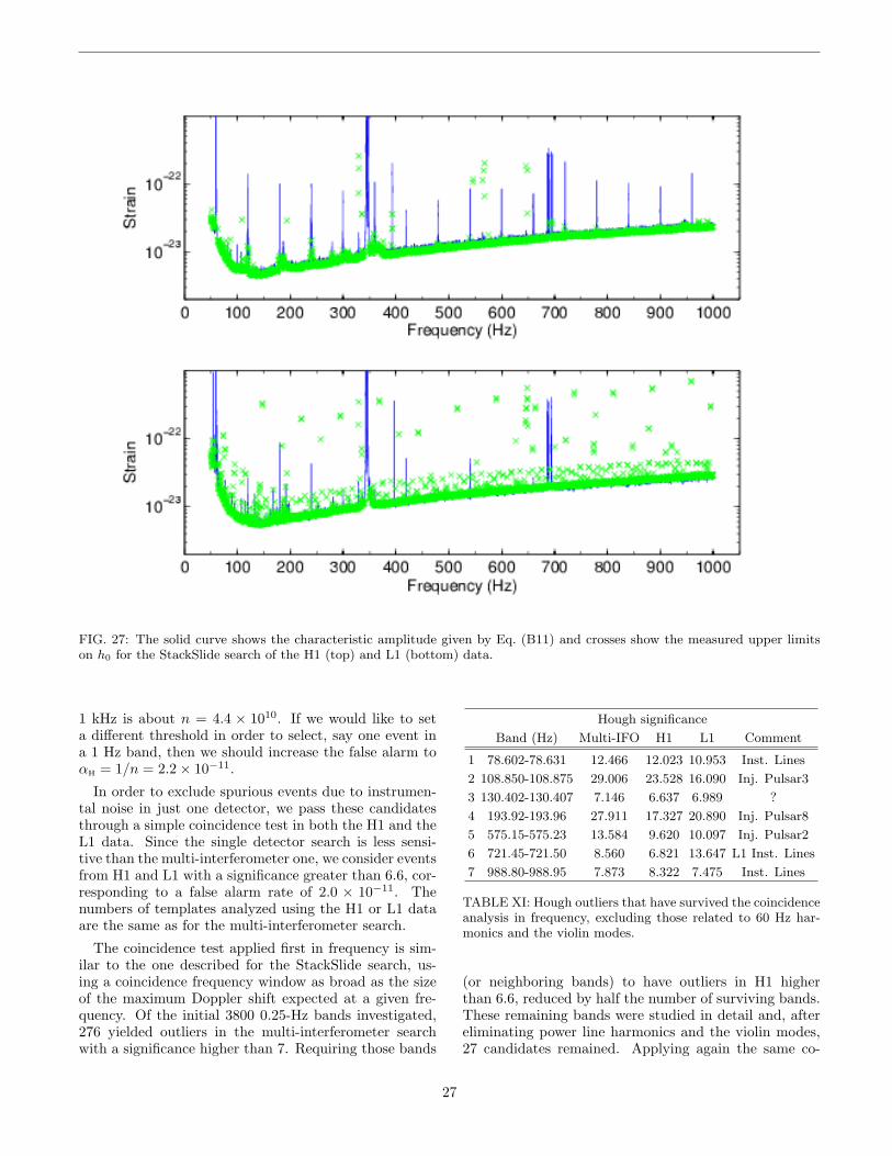
FIG. 27: The solid curve shows the characteristic amplitude given by Eq. (B11) and crosses show the measured upper limitson h0 for the StackSlide search of the H1 (top) and L1 (bottom) data.
1 kHz is about n = 4.4 × 10¹⁰. If we would like to seta different threshold in order to select, say one event ina 1 Hz band, then we should increase the false alarm toαH = 1/n = 2.2× 10⁻¹¹.
In order to exclude spurious events due to instrumen-tal noise in just one detector, we pass these candidatesthrough a simple coincidence test in both the H1 and theL1 data. Since the single detector search is less sensi-tive than the multi-interferometer one, we consider eventsfrom H1 and L1 with a significance greater than 6.6, cor-responding to a false alarm rate of 2.0 × 10⁻¹¹. Thenumbers of templates analyzed using the H1 or L1 dataare the same as for the multi-interferometer search.
The coincidence test applied first in frequency is sim-ilar to the one described for the StackSlide search, us-ing a coincidence frequency window as broad as the sizeof the maximum Doppler shift expected at a given fre-quency. Of the initial 3800 0.25-Hz bands investigated,276 yielded outliers in the multi-interferometer searchwith a significance higher than 7. Requiring those bands
Hough significance
Band (Hz) Multi-IFO H1 L1 Comment
1 78.602-78.631 12.466 12.023 10.953 Inst. Lines
2 108.850-108.875 29.006 23.528 16.090 Inj. Pulsar3
3 130.402-130.407 7.146 6.637 6.989 ?
4 193.92-193.96 27.911 17.327 20.890 Inj. Pulsar8
5 575.15-575.23 13.584 9.620 10.097 Inj. Pulsar2
6 721.45-721.50 8.560 6.821 13.647 L1 Inst. Lines
7 988.80-988.95 7.873 8.322 7.475 Inst. Lines
TABLE XI: Hough outliers that have survived the coincidenceanalysis in frequency, excluding those related to 60 Hz har-monics and the violin modes.
(or neighboring bands) to have outliers in H1 higherthan 6.6, reduced by half the number of surviving bands.These remaining bands were studied in detail and, aftereliminating power line harmonics and the violin modes,27 candidates remained. Applying again the same co-
27

FIG. 28: Relative contributions of the three interferometersin the Hough multi-interferometer search. The noise weightsare calculated in 1 Hz bands.
FIG. 29: The measured loudest significance in each 0.25 Hzfrom the Hough search of the multi-interferometer (top), H1(middle) and L1(bottom) data.
incidence test with the L1 data, we are left with only7 coincidence outliers that are listed on Table XI anddisplayed in Fig. 30.
Except for the third outlier, the coincidence can beattributed to instrumental lines in the detectors or tothe hardware pulsar injections. Table XII summarizes
FIG. 30: Hough significance of the outliers that have survivedthe coincidence analysis without considering the bands con-taminated with 60 Hz harmonics or the violin modes. Pointsare plotted only for multi-interferometer templates with sig-nificance greater than 7 and for single-interferometer tem-plates with significance greater than 6.6.
Detector s f0 (Hz) df/dt (Hz s−1) α (rad) δ (rad)
Multi-IFO 7.146 130.4028 −1.745× 10⁻⁹ 0.8798 -1.2385
H1 6.622 130.4039 −1.334× 10⁻⁹ 2.1889 0.7797
H1 6.637 130.4050 −1.334× 10⁻⁹ 2.0556 0.6115
L1 6.989 130.4067 −1.963× 10⁻⁹ 1.1690 -1.0104
TABLE XII: Parameters of the candidate events with a sig-nificance greater than 6.6 in the multi-interferometer, H1 andL1 data searches around the Hough outlier number 3. The pa-rameters correspond to the significance, frequency and spin-down for the reference time of the beginning of S4, and skylocations.
28
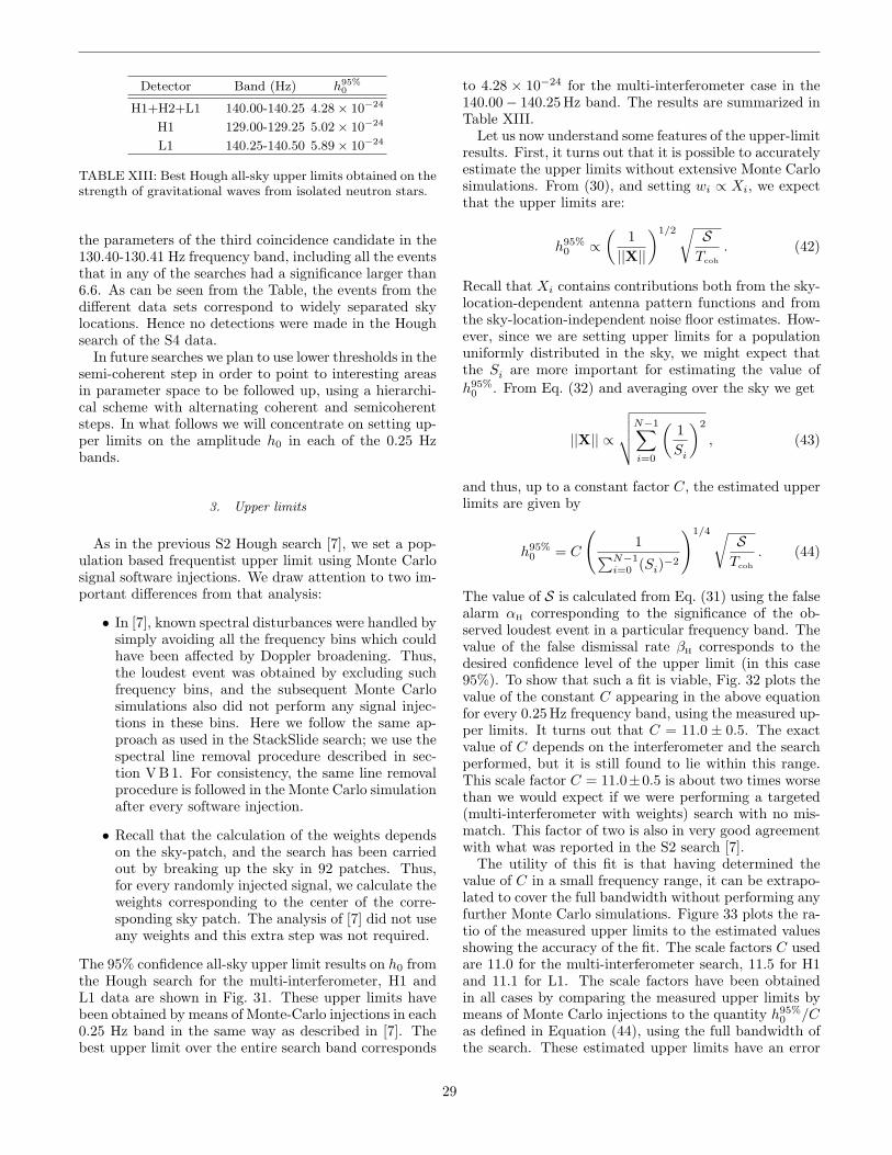
Detector Band (Hz) h95%0
H1+H2+L1 140.00-140.25 4.28× 10⁻²⁴
H1 129.00-129.25 5.02× 10⁻²⁴
L1 140.25-140.50 5.89× 10⁻²⁴
TABLE XIII: Best Hough all-sky upper limits obtained on thestrength of gravitational waves from isolated neutron stars.
the parameters of the third coincidence candidate in the130.40-130.41 Hz frequency band, including all the eventsthat in any of the searches had a significance larger than6.6. As can be seen from the Table, the events from thedifferent data sets correspond to widely separated skylocations. Hence no detections were made in the Houghsearch of the S4 data.
In future searches we plan to use lower thresholds in thesemi-coherent step in order to point to interesting areasin parameter space to be followed up, using a hierarchi-cal scheme with alternating coherent and semicoherentsteps. In what follows we will concentrate on setting up-per limits on the amplitude h0 in each of the 0.25 Hzbands.
3. Upper limits
As in the previous S2 Hough search [7], we set a pop-ulation based frequentist upper limit using Monte Carlosignal software injections. We draw attention to two im-portant differences from that analysis:
• In [7], known spectral disturbances were handled bysimply avoiding all the frequency bins which couldhave been affected by Doppler broadening. Thus,the loudest event was obtained by excluding suchfrequency bins, and the subsequent Monte Carlosimulations also did not perform any signal injec-tions in these bins. Here we follow the same ap-proach as used in the StackSlide search; we use thespectral line removal procedure described in sec-tion V B 1. For consistency, the same line removalprocedure is followed in the Monte Carlo simulationafter every software injection.
• Recall that the calculation of the weights dependson the sky-patch, and the search has been carriedout by breaking up the sky in 92 patches. Thus,for every randomly injected signal, we calculate theweights corresponding to the center of the corre-sponding sky patch. The analysis of [7] did not useany weights and this extra step was not required.
The 95% confidence all-sky upper limit results on h0 fromthe Hough search for the multi-interferometer, H1 andL1 data are shown in Fig. 31. These upper limits havebeen obtained by means of Monte-Carlo injections in each0.25 Hz band in the same way as described in [7]. Thebest upper limit over the entire search band corresponds
to 4.28 × 10⁻²⁴ for the multi-interferometer case in the140.00− 140.25 Hz band. The results are summarized inTable XIII.
Let us now understand some features of the upper-limitresults. First, it turns out that it is possible to accuratelyestimate the upper limits without extensive Monte Carlosimulations. From (30), and setting wi ∝ Xi, we expectthat the upper limits are:
h95%0 ∝
(1||X||
)1/2√ STcoh
. (42)
Recall that Xi contains contributions both from the sky-location-dependent antenna pattern functions and fromthe sky-location-independent noise floor estimates. How-ever, since we are setting upper limits for a populationuniformly distributed in the sky, we might expect thatthe Si are more important for estimating the value ofh95%
0 . From Eq. (32) and averaging over the sky we get
||X|| ∝
√√√√N−1∑i=0
(1Si
)2
, (43)
and thus, up to a constant factor C, the estimated upperlimits are given by
h95%0 = C
(1∑N−1
i=0 (Si)−2
)1/4√STcoh
. (44)
The value of S is calculated from Eq. (31) using the falsealarm αH corresponding to the significance of the ob-served loudest event in a particular frequency band. Thevalue of the false dismissal rate βH corresponds to thedesired confidence level of the upper limit (in this case95%). To show that such a fit is viable, Fig. 32 plots thevalue of the constant C appearing in the above equationfor every 0.25 Hz frequency band, using the measured up-per limits. It turns out that C = 11.0 ± 0.5. The exactvalue of C depends on the interferometer and the searchperformed, but it is still found to lie within this range.This scale factor C = 11.0±0.5 is about two times worsethan we would expect if we were performing a targeted(multi-interferometer with weights) search with no mis-match. This factor of two is also in very good agreementwith what was reported in the S2 search [7].
The utility of this fit is that having determined thevalue of C in a small frequency range, it can be extrapo-lated to cover the full bandwidth without performing anyfurther Monte Carlo simulations. Figure 33 plots the ra-tio of the measured upper limits to the estimated valuesshowing the accuracy of the fit. The scale factors C usedare 11.0 for the multi-interferometer search, 11.5 for H1and 11.1 for L1. The scale factors have been obtainedin all cases by comparing the measured upper limits bymeans of Monte Carlo injections to the quantity h95%
0 /Cas defined in Equation (44), using the full bandwidth ofthe search. These estimated upper limits have an error
29
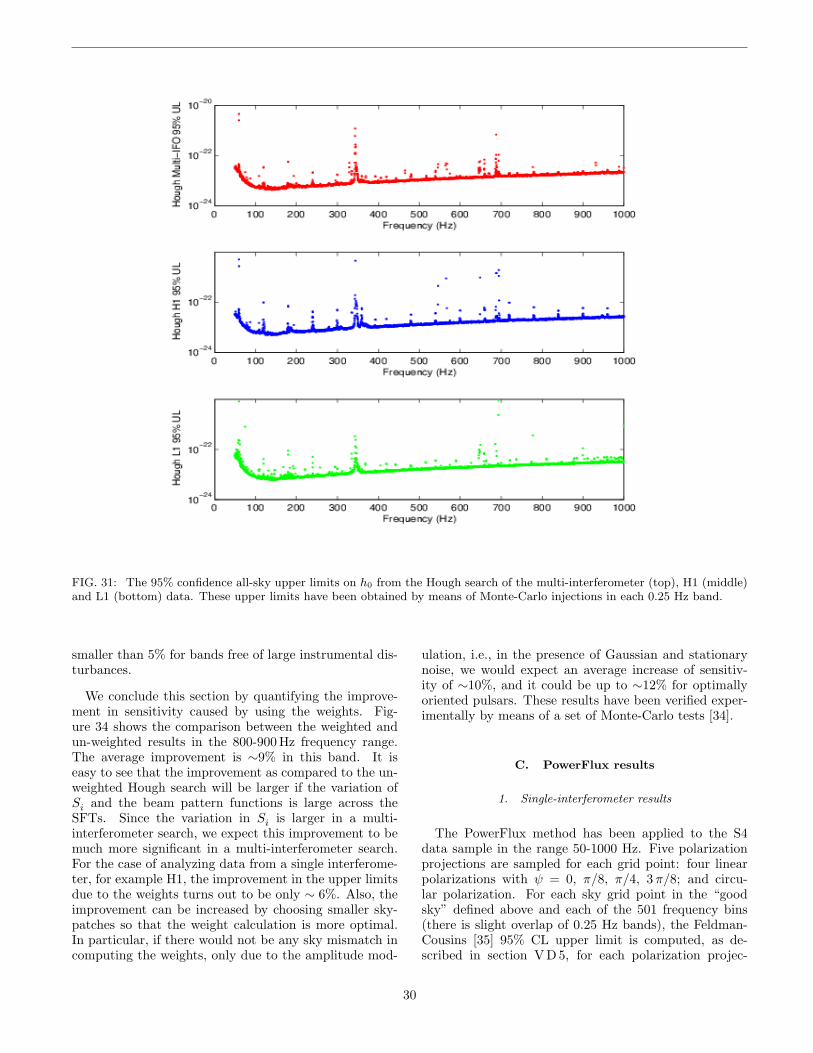
FIG. 31: The 95% confidence all-sky upper limits on h0 from the Hough search of the multi-interferometer (top), H1 (middle)and L1 (bottom) data. These upper limits have been obtained by means of Monte-Carlo injections in each 0.25 Hz band.
smaller than 5% for bands free of large instrumental dis-turbances.
We conclude this section by quantifying the improve-ment in sensitivity caused by using the weights. Fig-ure 34 shows the comparison between the weighted andun-weighted results in the 800-900 Hz frequency range.The average improvement is ∼9% in this band. It iseasy to see that the improvement as compared to the un-weighted Hough search will be larger if the variation ofSi and the beam pattern functions is large across theSFTs. Since the variation in Si is larger in a multi-interferometer search, we expect this improvement to bemuch more significant in a multi-interferometer search.For the case of analyzing data from a single interferome-ter, for example H1, the improvement in the upper limitsdue to the weights turns out to be only ∼ 6%. Also, theimprovement can be increased by choosing smaller sky-patches so that the weight calculation is more optimal.In particular, if there would not be any sky mismatch incomputing the weights, only due to the amplitude mod-
ulation, i.e., in the presence of Gaussian and stationarynoise, we would expect an average increase of sensitiv-ity of ∼10%, and it could be up to ∼12% for optimallyoriented pulsars. These results have been verified exper-imentally by means of a set of Monte-Carlo tests [34].
C. PowerFlux results
1. Single-interferometer results
The PowerFlux method has been applied to the S4data sample in the range 50-1000 Hz. Five polarizationprojections are sampled for each grid point: four linearpolarizations with ψ = 0, π/8, π/4, 3π/8; and circu-lar polarization. For each sky grid point in the “goodsky” defined above and each of the 501 frequency bins(there is slight overlap of 0.25 Hz bands), the Feldman-Cousins [35] 95% CL upper limit is computed, as de-scribed in section V D 5, for each polarization projec-
30
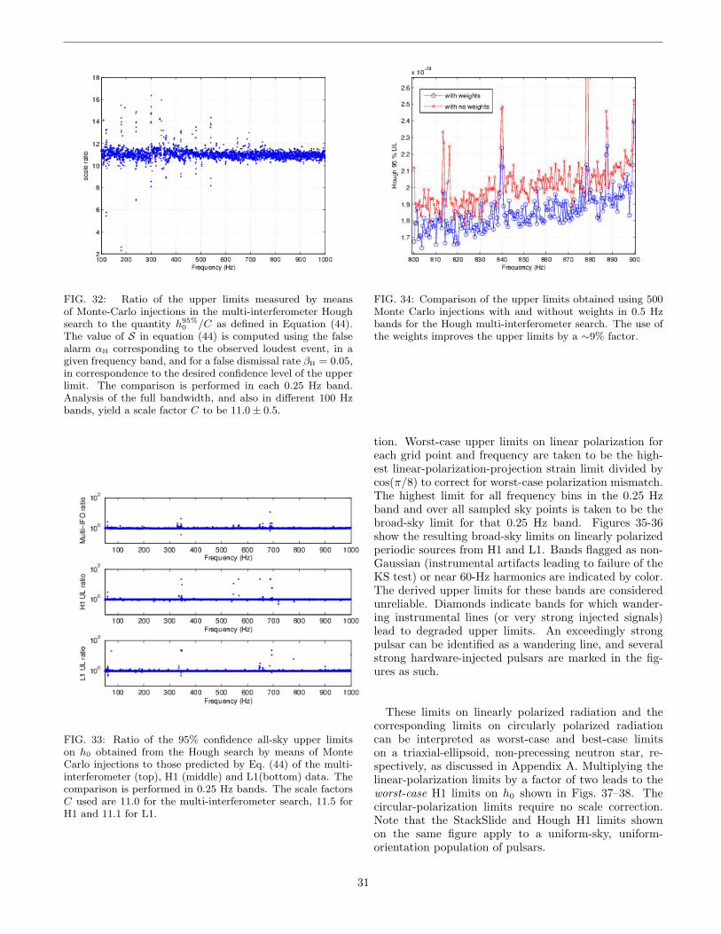
FIG. 32: Ratio of the upper limits measured by meansof Monte-Carlo injections in the multi-interferometer Houghsearch to the quantity h95%
0 /C as defined in Equation (44).The value of S in equation (44) is computed using the falsealarm αH corresponding to the observed loudest event, in agiven frequency band, and for a false dismissal rate βH = 0.05,in correspondence to the desired confidence level of the upperlimit. The comparison is performed in each 0.25 Hz band.Analysis of the full bandwidth, and also in different 100 Hzbands, yield a scale factor C to be 11.0± 0.5.
FIG. 33: Ratio of the 95% confidence all-sky upper limitson h0 obtained from the Hough search by means of MonteCarlo injections to those predicted by Eq. (44) of the multi-interferometer (top), H1 (middle) and L1(bottom) data. Thecomparison is performed in 0.25 Hz bands. The scale factorsC used are 11.0 for the multi-interferometer search, 11.5 forH1 and 11.1 for L1.
FIG. 34: Comparison of the upper limits obtained using 500Monte Carlo injections with and without weights in 0.5 Hzbands for the Hough multi-interferometer search. The use ofthe weights improves the upper limits by a ∼9% factor.
tion. Worst-case upper limits on linear polarization foreach grid point and frequency are taken to be the high-est linear-polarization-projection strain limit divided bycos(π/8) to correct for worst-case polarization mismatch.The highest limit for all frequency bins in the 0.25 Hzband and over all sampled sky points is taken to be thebroad-sky limit for that 0.25 Hz band. Figures 35-36show the resulting broad-sky limits on linearly polarizedperiodic sources from H1 and L1. Bands flagged as non-Gaussian (instrumental artifacts leading to failure of theKS test) or near 60-Hz harmonics are indicated by color.The derived upper limits for these bands are consideredunreliable. Diamonds indicate bands for which wander-ing instrumental lines (or very strong injected signals)lead to degraded upper limits. An exceedingly strongpulsar can be identified as a wandering line, and severalstrong hardware-injected pulsars are marked in the fig-ures as such.
These limits on linearly polarized radiation and thecorresponding limits on circularly polarized radiationcan be interpreted as worst-case and best-case limitson a triaxial-ellipsoid, non-precessing neutron star, re-spectively, as discussed in Appendix A. Multiplying thelinear-polarization limits by a factor of two leads to theworst-case H1 limits on h0 shown in Figs. 37–38. Thecircular-polarization limits require no scale correction.Note that the StackSlide and Hough H1 limits shownon the same figure apply to a uniform-sky, uniform-orientation population of pulsars.
31
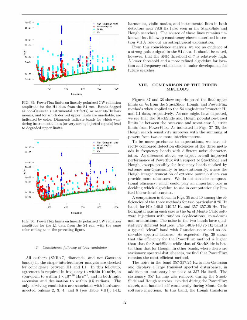
FIG. 35: PowerFlux limits on linearly polarized CW radiationamplitude for the H1 data from the S4 run. Bands flaggedas non-Gaussian (instrumental artifacts) or near 60-Hz har-monics, and for which derived upper limits are unreliable, areindicated by color. Diamonds indicate bands for which wan-dering instrumental lines (or very strong injected signals) leadto degraded upper limits.
FIG. 36: PowerFlux limits on linearly polarized CW radiationamplitude for the L1 data from the S4 run, with the samecolor coding as in the preceding figure.
2. Coincidence followup of loud candidates
All outliers (SNR>7, diamonds, and non-Gaussianbands) in the single-interferometer analysis are checkedfor coincidence between H1 and L1. In this followup,agreement is required in frequency to within 10 mHz, inspin-down to within 1× 10⁻¹⁰ Hz s−1, and in both rightascension and declination to within 0.5 radians. Theonly surviving candidates are associated with hardware-injected pulsars 2, 3, 4, and 8 (see Table VIII), 1-Hz
harmonics, violin modes, and instrumental lines in bothdetectors near 78.6 Hz (also seen in the StackSlide andHough searches). The source of these lines remains un-known, but followup consistency checks described in sec-tion VII A rule out an astrophysical explanation.
From this coincidence analysis, we see no evidence ofa strong pulsar signal in the S4 data. It should be noted,however, that the SNR threshold of 7 is relatively high.A lower threshold and a more refined algorithm for loca-tion and frequency coincidence is under development forfuture searches.
VIII. COMPARISON OF THE THREEMETHODS
Figures 37 and 38 show superimposed the final upperlimits on h0 from the StackSlide, Hough, and PowerFluxmethods when applied to the S4 single-interferometer H1and L1 data, respectively. As one might have expected,we see that the StackSlide and Hough population-basedlimits lie between the best-case and worst-case h0 strictlimits from PowerFlux. As indicated in Figs. 37–38, theHough search sensitivity improves with the summing ofpowers from two or more interferometers.
To be more precise as to expectations, we have di-rectly compared detection efficiencies of the three meth-ods in frequency bands with different noise character-istics. As discussed above, we expect overall improvedperformance of Powerflux with respect to StackSlide andHough, except possibly for frequency bands marked byextreme non-Gaussianity or non-stationarity, where theHough integer truncation of extreme power outliers canprovide more robustness. We do not consider computa-tional efficiency, which could play an important role indeciding which algorithm to use in computationally lim-ited hierarchical searches.
A comparison is shown in Figs. 39 and 40 among the ef-ficiencies of the three methods for two particular 0.25 Hzbands for H1: 140.5–140.75 Hz and 357–357.25 Hz. Thehorizontal axis in each case is the h0 of Monte Carlo soft-ware injections with random sky-locations, spin-downsand orientations. The noise in the two bands have qual-itatively different features. The 140.5-140.75 Hz band isa typical “clean” band with Gaussian noise and no ob-servable spectral features. As expected, Fig. 39 showsthat the efficiency for the PowerFlux method is higherthan that for StackSlide, while that of StackSlide is bet-ter than that for Hough. In other bands, where there arestationary spectral disturbances, we find that PowerFluxremains the most efficient method.
The noise in the band 357-357.25 Hz is non-Gaussianand displays a large transient spectral disturbance, inaddition to stationary line noise at 357 Hz itself. Thestationary 357 Hz line was removed during the Stack-Slide and Hough searches, avoided during the PowerFluxsearch, and handled self-consistently during Monte Carlosoftware injections. In this band, the Hough transform
32
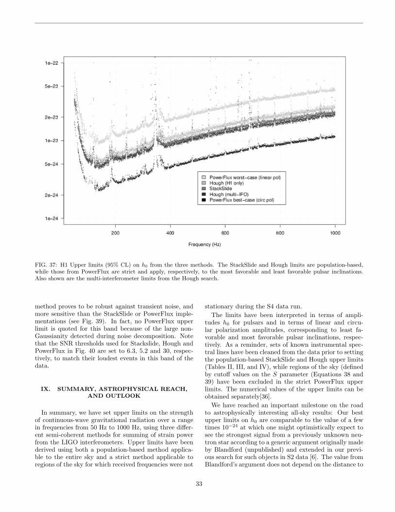
FIG. 37: H1 Upper limits (95% CL) on h0 from the three methods. The StackSlide and Hough limits are population-based,while those from PowerFlux are strict and apply, respectively, to the most favorable and least favorable pulsar inclinations.Also shown are the multi-interferometer limits from the Hough search.
method proves to be robust against transient noise, andmore sensitive than the StackSlide or PowerFlux imple-mentations (see Fig. 39). In fact, no PowerFlux upperlimit is quoted for this band because of the large non-Gaussianity detected during noise decomposition. Notethat the SNR thresholds used for Stackslide, Hough andPowerFlux in Fig. 40 are set to 6.3, 5.2 and 30, respec-tively, to match their loudest events in this band of thedata.
IX. SUMMARY, ASTROPHYSICAL REACH,AND OUTLOOK
In summary, we have set upper limits on the strengthof continuous-wave gravitational radiation over a rangein frequencies from 50 Hz to 1000 Hz, using three differ-ent semi-coherent methods for summing of strain powerfrom the LIGO interferometers. Upper limits have beenderived using both a population-based method applica-ble to the entire sky and a strict method applicable toregions of the sky for which received frequencies were not
stationary during the S4 data run.The limits have been interpreted in terms of ampli-
tudes h0 for pulsars and in terms of linear and circu-lar polarization amplitudes, corresponding to least fa-vorable and most favorable pulsar inclinations, respec-tively. As a reminder, sets of known instrumental spec-tral lines have been cleaned from the data prior to settingthe population-based StackSlide and Hough upper limits(Tables II, III, and IV), while regions of the sky (definedby cutoff values on the S parameter (Equations 38 and39) have been excluded in the strict PowerFlux upperlimits. The numerical values of the upper limits can beobtained separately[36].
We have reached an important milestone on the roadto astrophysically interesting all-sky results: Our bestupper limits on h0 are comparable to the value of a fewtimes 10−24 at which one might optimistically expect tosee the strongest signal from a previously unknown neu-tron star according to a generic argument originally madeby Blandford (unpublished) and extended in our previ-ous search for such objects in S2 data [6]. The value fromBlandford’s argument does not depend on the distance to
33
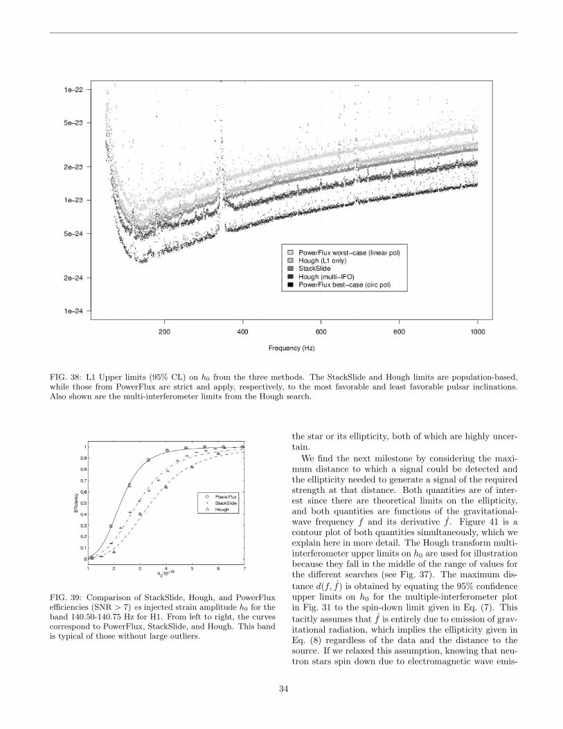
FIG. 38: L1 Upper limits (95% CL) on h0 from the three methods. The StackSlide and Hough limits are population-based,while those from PowerFlux are strict and apply, respectively, to the most favorable and least favorable pulsar inclinations.Also shown are the multi-interferometer limits from the Hough search.
FIG. 39: Comparison of StackSlide, Hough, and PowerFluxefficiencies (SNR > 7) vs injected strain amplitude h0 for theband 140.50-140.75 Hz for H1. From left to right, the curvescorrespond to PowerFlux, StackSlide, and Hough. This bandis typical of those without large outliers.
the star or its ellipticity, both of which are highly uncer-tain.
We find the next milestone by considering the maxi-mum distance to which a signal could be detected andthe ellipticity needed to generate a signal of the requiredstrength at that distance. Both quantities are of inter-est since there are theoretical limits on the ellipticity,and both quantities are functions of the gravitational-wave frequency f and its derivative f . Figure 41 is acontour plot of both quantities simultaneously, which weexplain here in more detail. The Hough transform multi-interferometer upper limits on h0 are used for illustrationbecause they fall in the middle of the range of values forthe different searches (see Fig. 37). The maximum dis-tance d(f, f) is obtained by equating the 95% confidenceupper limits on h0 for the multiple-interferometer plotin Fig. 31 to the spin-down limit given in Eq. (7). Thistacitly assumes that f is entirely due to emission of grav-itational radiation, which implies the ellipticity given inEq. (8) regardless of the data and the distance to thesource. If we relaxed this assumption, knowing that neu-tron stars spin down due to electromagnetic wave emis-
34
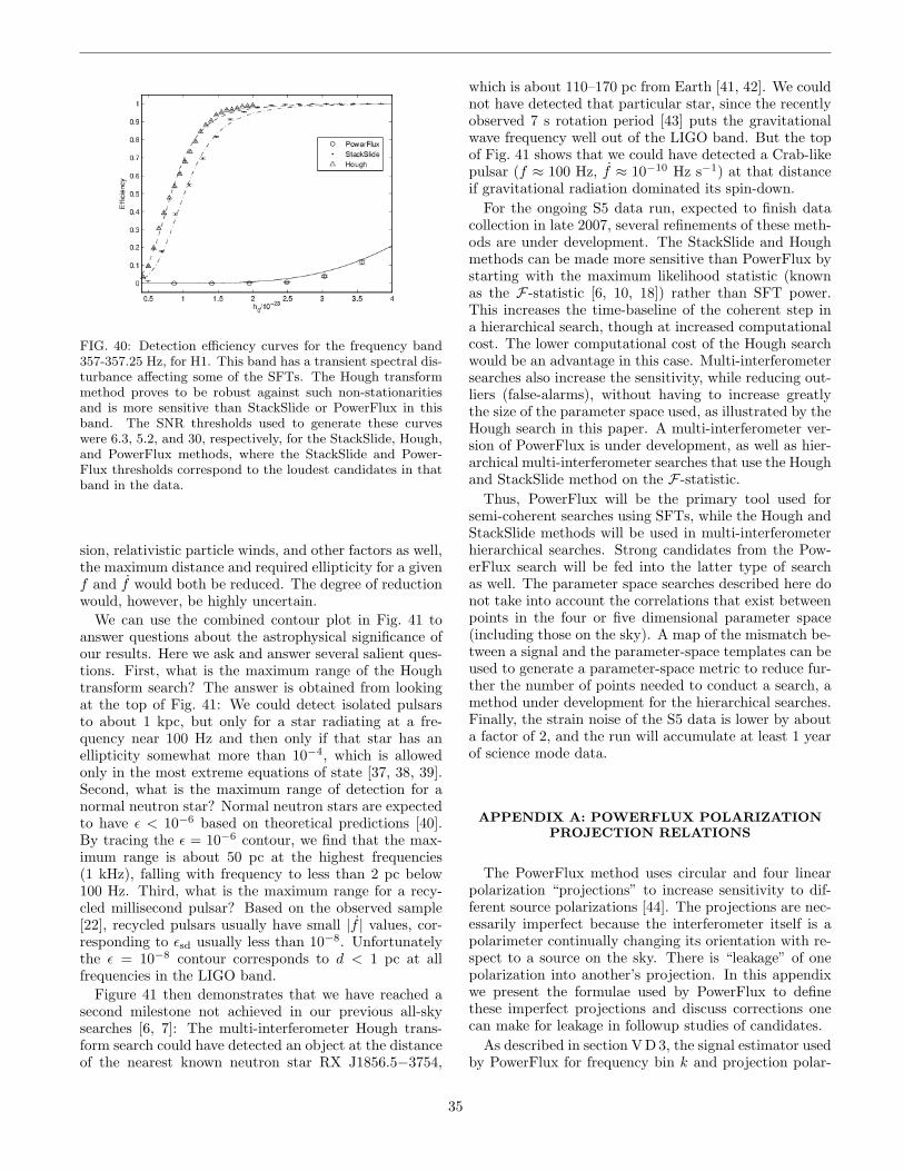
FIG. 40: Detection efficiency curves for the frequency band357-357.25 Hz, for H1. This band has a transient spectral dis-turbance affecting some of the SFTs. The Hough transformmethod proves to be robust against such non-stationaritiesand is more sensitive than StackSlide or PowerFlux in thisband. The SNR thresholds used to generate these curveswere 6.3, 5.2, and 30, respectively, for the StackSlide, Hough,and PowerFlux methods, where the StackSlide and Power-Flux thresholds correspond to the loudest candidates in thatband in the data.
sion, relativistic particle winds, and other factors as well,the maximum distance and required ellipticity for a givenf and f would both be reduced. The degree of reductionwould, however, be highly uncertain.
We can use the combined contour plot in Fig. 41 toanswer questions about the astrophysical significance ofour results. Here we ask and answer several salient ques-tions. First, what is the maximum range of the Houghtransform search? The answer is obtained from lookingat the top of Fig. 41: We could detect isolated pulsarsto about 1 kpc, but only for a star radiating at a fre-quency near 100 Hz and then only if that star has anellipticity somewhat more than 10−4, which is allowedonly in the most extreme equations of state [37, 38, 39].Second, what is the maximum range of detection for anormal neutron star? Normal neutron stars are expectedto have ε < 10−6 based on theoretical predictions [40].By tracing the ε = 10−6 contour, we find that the max-imum range is about 50 pc at the highest frequencies(1 kHz), falling with frequency to less than 2 pc below100 Hz. Third, what is the maximum range for a recy-cled millisecond pulsar? Based on the observed sample[22], recycled pulsars usually have small |f | values, cor-responding to εsd usually less than 10−8. Unfortunatelythe ε = 10−8 contour corresponds to d < 1 pc at allfrequencies in the LIGO band.
Figure 41 then demonstrates that we have reached asecond milestone not achieved in our previous all-skysearches [6, 7]: The multi-interferometer Hough trans-form search could have detected an object at the distanceof the nearest known neutron star RX J1856.5−3754,
which is about 110–170 pc from Earth [41, 42]. We couldnot have detected that particular star, since the recentlyobserved 7 s rotation period [43] puts the gravitationalwave frequency well out of the LIGO band. But the topof Fig. 41 shows that we could have detected a Crab-likepulsar (f ≈ 100 Hz, f ≈ 10−10 Hz s−1) at that distanceif gravitational radiation dominated its spin-down.
For the ongoing S5 data run, expected to finish datacollection in late 2007, several refinements of these meth-ods are under development. The StackSlide and Houghmethods can be made more sensitive than PowerFlux bystarting with the maximum likelihood statistic (knownas the F-statistic [6, 10, 18]) rather than SFT power.This increases the time-baseline of the coherent step ina hierarchical search, though at increased computationalcost. The lower computational cost of the Hough searchwould be an advantage in this case. Multi-interferometersearches also increase the sensitivity, while reducing out-liers (false-alarms), without having to increase greatlythe size of the parameter space used, as illustrated by theHough search in this paper. A multi-interferometer ver-sion of PowerFlux is under development, as well as hier-archical multi-interferometer searches that use the Houghand StackSlide method on the F-statistic.
Thus, PowerFlux will be the primary tool used forsemi-coherent searches using SFTs, while the Hough andStackSlide methods will be used in multi-interferometerhierarchical searches. Strong candidates from the Pow-erFlux search will be fed into the latter type of searchas well. The parameter space searches described here donot take into account the correlations that exist betweenpoints in the four or five dimensional parameter space(including those on the sky). A map of the mismatch be-tween a signal and the parameter-space templates can beused to generate a parameter-space metric to reduce fur-ther the number of points needed to conduct a search, amethod under development for the hierarchical searches.Finally, the strain noise of the S5 data is lower by abouta factor of 2, and the run will accumulate at least 1 yearof science mode data.
APPENDIX A: POWERFLUX POLARIZATIONPROJECTION RELATIONS
The PowerFlux method uses circular and four linearpolarization “projections” to increase sensitivity to dif-ferent source polarizations [44]. The projections are nec-essarily imperfect because the interferometer itself is apolarimeter continually changing its orientation with re-spect to a source on the sky. There is “leakage” of onepolarization into another’s projection. In this appendixwe present the formulae used by PowerFlux to definethese imperfect projections and discuss corrections onecan make for leakage in followup studies of candidates.
As described in section V D 3, the signal estimator usedby PowerFlux for frequency bin k and projection polar-
35
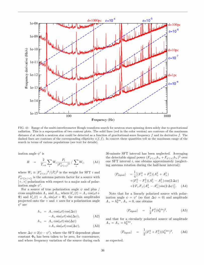
FIG. 41: Range of the multi-interferometer Hough transform search for neutron stars spinning down solely due to gravitationalradiation. This is a superposition of two contour plots. The solid lines (red in the color version) are contours of the maximum
distance d at which a neutron star could be detected as a function of gravitational-wave frequency f and its derivative f . Thedashed lines are contours of the corresponding ellipticity ε(f, f). In concert these quantities tell us the maximum range of thesearch in terms of various populations (see text for details).
ization angle ψ′ is
R =2Tcoh
∑i
WiPi
|F iψ′(+)|2/∑i
Wi, (A1)
where Wi ≡ |F iψ′(+)|4/(Pi)2 is the weight for SFT i and
F iψ′([+/×]) is the antenna pattern factor for a source with[+,×] polarization with respect to a major axis of polar-ization angle ψ′.
For a source of true polarization angle ψ and plus /cross amplitudes A+ and A×, where h′+(t) = A+ cos(ωt+Φ) and h′×(t) = A× sin(ωt + Φ), the strain amplitudesprojected onto the + and × axes for a polarization angleψ′ are
h+ = A+ cos(ωt) cos(∆ψ)−A× sin(ωt) sin(∆ψ), (A2)
h× = A+ cos(ωt) sin(∆ψ)+A× sin(ωt) cos(∆ψ), (A3)
where ∆ψ ≡ 2(ψ − ψ′), where the SFT-dependent phaseconstant Φ0 has been taken to be zero, for convenience,and where frequency variation of the source during each
30-minute SFT interval has been neglected. Averagingthe detectable signal power (Fψ′(+)h+ +Fψ′(×)h×)2 overone SFT interval i, one obtains approximately (neglect-ing antenna rotation during the half-hour interval):
〈Psignal〉 =14[(F 2
+ + F 2×)(A2
+ +A2×)
+(F 2+ − F 2
×)(A2+ −A2
×) cos(2 ∆ψ)
+2F+F×(A2+ −A2
×) sin(2 ∆ψ)]. (A4)
Note that for a linearly polarized source with polar-ization angle ψ = ψ′ (so that ∆ψ = 0) and amplitudeA+ = hLin
0 , A× = 0, one obtains
〈Psignal〉 =12F 2
+(hLin0 )2, (A5)
and that for a circularly polarized source of amplitudeA+ = A× = hCirc
0 ,
〈Psignal〉 =12
(F 2+ + F 2
×)(hCirc0 )2, (A6)
as expected.
36
For an average of powers from many SFT’s, weightedaccording to detector noise and antenna pattern via Wi,the expectation value of the signal estimator depends on
〈PDet〉 = 〈Psignal〉+ 〈n(ψ′)2〉+2〈Psignaln(ψ′)〉, (A7)
where ni is the expected power from noise alone, where〈Psignaln〉 is assumed to vanish (signal uncorrelated withnoise), and where the frequency bin index k is omittedfor simplicity.
For a true source with parameters ψ, A+, and A×, thisexpectation value can be written:
〈PDet〉 = 〈n(ψ′)2〉
+14[(1 + β2)(A2
+ +A2×)
+(1− β2)(A2+ −A2
×) cos(2∆ψ)
+2β1 (A2+ −A2
×) sin(2∆ψ)], (A8)
where the correction coefficients
β1 =∑iWi F×/F+∑
iWi, (A9)
β2 =∑iWi F
2×/F
2+∑
iWi, (A10)
depend implicitly on ψ′ through F+ and F×.For a linearly polarized source with polarization angle
ψ = ψ′, one obtains
〈PDet〉 = 〈n(ψ′)2〉+12
(hLin0 )2 (A11)
and for a circularly polarized source one obtains:
〈PDet〉 = 〈n(ψ′)2〉+12
(hCirc0 )2(1 + β2). (A12)
These formulae permit corrections for polarizationleakage to be applied for a hypothetical source, allow-ing for estimation of ψ, A+, and A× from a sampling ofpolarization projection measurements. In practice, how-ever, the calculation of the β coefficients is computation-ally costly in an all-sky search and is disabled by default.Instead, upper limits on linearly polarized sources (worst-case pulsar inclination) are derived from the maximumlimit over all four linear polarization projections, as de-scribed in section V D 3. In followup investigations ofoutliers, however, these formulae permit greater discrim-ination of candidates, now in use for PowerFlux searchesof the data from the ongoing S5 data run.
APPENDIX B: STACKSLIDE POWER ANDSTATISTICS
a. Approximate Form For The StackSlide Power
It is useful to have an analytic approximation for theStackSlide Power P . For a single SFT (dropping the
SFT index i) expressing the phase in a first-order Taylorexpansion about the midpoint time, t1/2, of the intervalused to generate an SFT, we can write
φ(t) ∼= φ1/2 + 2πf1/2(t− t1/2) , (B1)
where φ1/2 and f1/2 are the phase and frequency at timet1/2. Treating the values of F+ and F× as constants equalto their values at time t1/2, the signal strain at discretetime tj is approximately,
hj ∼= F+A+cos(φ0 + 2πf1/2tj)+F×A×sin(φ0 + 2πf1/2tj) , (B2)
where j = 0 gives the start time of the SFT, and φ0 isthe approximate phase at the start of the SFT (not theinitial phase at the start of the observation), i.e.,
φ0 ≡ φ1/2 − 2πf1/2(Tcoh/2) . (B3)
Using these approximations, the Discrete Fourier Trans-form, given by Eq. (12), of hj is
hkTcoh
∼= eiφ0
[F+A+
2− i
F×A×2
][sin(2π∆κ)
2π∆κ
+i1− cos(2π∆κ)
2π∆κ
], (B4)
where ∆κ ≡ κ − k and κ ≡ f1/2Tcoh is usually not aninteger. Equation (B4) holds for 0 < κ < M/2 and|κ − k| << M , which is true for all of the frequenciesover which we search.
If the discrete time samples of the data from the de-tector consist of a signal plus noise the expected value ofP is approximated by
P ∼= P0 +12〈d2〉 , (B5)
where the mean value of P0 is 1 and its standard deviationis 1/
√N due to the normalization used, and
〈d2〉 ∼=
[A2
+
⟨F 2
+
Sk
sin2(π∆κ)π2∆κ2
⟩
+A2×
⟨F 2×Sk
sin2(π∆κ)π2∆κ2
⟩]Tcoh , (B6)
is an approximate form for the square of the optimal SNRdefined in Eq. (71) in reference [18] averaged over SFTs(i.e., the angle brackets on 〈d2〉 represent an average overSFTs) and where for each SFT the index k is the nearestinteger value to κ. Thus, the relevant range for ∆κ is0 to 0.5, corresponding to a frequency mismatch of 0 to1/2 of an SFT frequency bin.
37
b. StackSlide Statistics
It can be seen from Eq. (16) that, for Gaussian noisein the absence of a signal, 2NP is a χ2 variable with 2Ndegrees of freedom [15]. Thus, the quantity
% ≡ 2NP (B7)
follows the χ2 distribution:
P(%;N)d% =1
2NΓ(N)%N−1e−%/2d% . (B8)
When a signal is present, % follows a non-central χ2 distri-bution with 2N degrees of freedom and a non-centralityparameter N〈d2〉 such that
P(%;N〈d2〉)d% =
IN−1
(√%N〈d2〉
)(N〈d2〉)N−1
%N−1
2 e−(%+N〈d2〉)/2d% , (B9)
where the form given here is based on that given in [28],and IN−1 is the modified Bessel function of the first kindand order N − 1.
The distribution described by Eqs. (B8) and (B9) canbe used to find the minimum optimal signal-to-noise ra-tio that can be detected using the StackSlide search forfixed false alarm and false dismissal rates, for a targetedsearch. For a 1% false alarm rate, a 10% false dis-missal rate, and large N Eqs. (B7) and (B9) give 〈d2〉 =7.385/
√N (See also [15]), while averaging Eq. (B6) in-
dependently over the source sky position, inclination an-gle, polarization angle, and mismatch in frequency gives〈d2〉 = 0.7737(4/25)(h2
0Tcoh/S) (see also Eq. 5.35 in [10]). Equating these and solving for h0, the characteris-tic amplitude for a targeted StackSlide search with a 1%false-alarm rate, 10% false-dismissal rate is:
〈h0〉targeted = 7.7√S/(TcohT
∗obs)
1/4 , (B10)
where T ∗obs = NTcoh is the actual duration of the data,which is shorter than the total observation time, Tobs,because gaps exist in the data for times when the detec-tors were not operating in science mode. Comparing thisexpression with Eq. 5.35 in [10] the StackSlide character-istic amplitude given in Eq. (B10) is found to be about10% lower than a similar estimate for the standard Houghsearch. Note that in this paper an improved version ofthe Hough method is presented. Also, in this paper anall-sky search for the loudest StackSlide Power is car-ried out, covering up to 1.88 × 10⁹ templates, and onlythe loudest StackSlide Power is returned from the search,corresponding to a false alarm rate of 5.32× 10⁻¹⁰. Fur-thermore, the upper limits are found by injecting a familyof signals, each of which has a StackSlide Power drawnfrom a different noncentral chi-squared distribution. Us-ing the results from Sec. VII, for an all-sky StackSlidesearch the 95% confidence all-sky upper limits are foundempirically to be approximately given by:
〈h0〉all−sky = 23√S/(TcohT
∗obs)
1/4 . (B11)
III. ACKNOWLEDGMENTS
The authors gratefully acknowledge the support of theUnited States National Science Foundation for the con-struction and operation of the LIGO Laboratory and theParticle Physics and Astronomy Research Council of theUnited Kingdom, the Max-Planck-Society and the Stateof Niedersachsen/Germany for support of the construc-tion and operation of the GEO600 detector. The authorsalso gratefully acknowledge the support of the research bythese agencies and by the Australian Research Council,the Natural Sciences and Engineering Research Coun-cil of Canada, the Council of Scientific and IndustrialResearch of India, the Department of Science and Tech-nology of India, the Spanish Ministerio de Educacion yCiencia, The National Aeronautics and Space Adminis-tration, the John Simon Guggenheim Foundation, theAlexander von Humboldt Foundation, the LeverhulmeTrust, the David and Lucile Packard Foundation, the Re-search Corporation, and the Alfred P. Sloan Foundation.This document has been assigned LIGO Laboratory doc-ument number LIGO-P060010-05-Z.
38
[1] A. Abramovici et al., Science 256, 325 (1992).[2] B. Barish and R. Weiss, Phys. Today 52, 44 (1999).[3] B. Abbott et al.(The LIGO Scientific Collaboration),
Phys. Rev. D 69 102001 (2004).[4] B. Abbott et al.(The LIGO Scientific Collaboration), M.
Kramer, and A. G. Lyne, Phys. Rev. Lett. 94 181103(2005).
[5] B. Abbott et al.(The LIGO Scientific Collaboration), M.Kramer, and A. G. Lyne, Phys Rev. D 76, 042001 (2007).
[6] B. Abbott et al.(The LIGO Scientific Collaboration), toappear in Phys. Rev. D, gr-qc/0605028 (2006).
[7] B. Abbott et al. (The LIGO Scientific Collaboration),Phys. Rev. D 72, 102004 (2005).
[8] The Einstein@Home project is built upon the BOINC(Berkeley Open Infrastructure for Network Computing)architecture described at http://boinc.berkeley.edu/.
[9] Results from the distributed computing project Ein-stein@Home can be found athttp://einstein.phys.uwm.edu/.
[10] B. Krishnan, A.M. Sintes, M.A. Papa, B.F. Schutz, S.Frasca, and C. Palomba, Phys.Rev. D 70, 082001 (2004).
[11] M.A. Papa, B.F. Schutz, A.M. Sintes, in Gravitationalwaves: A challenge to theoretical astrophysics, ICTP Lec-ture Notes Series, Vol. III, edited by V. Ferrari, J.C.Miller, L. Rezzolla (Italy 2001) p. 431.
[12] P. Brady, T. Creighton, Phys.Rev. D 61, 082001 (2000)[13] C. Cutler, I. Gholami, and B. Krishnan, Phys.Rev. D 72,
042004 (2005).[14] P. Brady, T. Creighton, C. Cutler and B.F. Schutz, Phys.
Rev. D 57, 2101 (1998).[15] G. Mendell and M. Landry, “StackSlide and Hough
Search SNR and Statistics”, LIGO technical documentLIGO-T050003 (2005), available inhttp://admdbsrv.ligo.caltech.edu/dcc/.
[16] C. Palomba, P. Astone, S. Frasca, Class. Quant. Grav.22, S1255 (2005).
[17] V. Dergachev, “Description of PowerFlux Algorithmsand Implementation”, LIGO technical document LIGO-T050186 (2005), available inhttp://admdbsrv.ligo.caltech.edu/dcc/.
[18] P. Jaranowski, A. Krolak, and B.F. Schutz, Phys. Rev.D 58, (1998) 063001.
[19] D. Sigg (for the LSC), Class. Quant. Grav. 23, S51(2006).
[20] LSC Algorithms and LALapps Applications software li-braries available athttp://www.lsc-group.phys.uwm.edu/daswg/.
[21] C. Palomba, Mon. Not. R. Astron. Soc. 359, 1150 (2005).[22] R. N. Manchester, G. B. Hobbs, A. Teoh and
M. Hobbs, Astron. J. 129, 1993 (2005). See alsohttp://www.atnf.csiro.au/research/pulsar/psrcat/.
[23] S.D. Mohanty, Class. Quantum. Grav. 19, 1513 (2002).[24] S.D. Mohanty, S. Mukherjee Class. Quantum. Grav. 19,
1471 (2002).[25] B. Krishnan, Bias in the estimator of the median, LIGO
technical document T040144 (2004), available inhttp://admdbsrv.ligo.caltech.edu/dcc/.
[26] X. Siemens et al, Class. Quant. Grav. 21, S1723 (2004).[27] A. Dietz et al., “Calibration of the LIGO Detectors for
S4”, LIGO technical document LIGO-T050262 (2005),available in
http://admdbsrv.ligo.caltech.edu/dcc/.[28] P. Jaranowski, A. Krolak, Phys. Rev. D 61 062001
(2000).[29] The condor package is available at
http://www.cs.wisc.edu/condor/.[30] The Matlab program is available at
http://www.mathworks.com.[31] P.V.C. Hough, In International Conference on High En-
ergy Accelerators and Instrumentation, CERN (1959).[32] P.V.C. Hough, U. S. Patent 3,069,654, 1962.[33] J. Illingworth and J. Kittler, Computer Vision, Graphics,
and Image Processing 44, 87 (1988).[34] B. Krishnan and A. M. Sintes, Hough search with im-
proved sensitivity, LIGO technical document T070124(2007), available inhttp://admdbsrv.ligo.caltech.edu/dcc/.
[35] G. J. Feldman and R. D. Cousins, Phys.Rev. D57, 3873(1998).
[36] See EPAPS Document No. [number will be inserted bypublisher] for numerical values of upper limits derived foreach method in 0.25-Hz bands in the range 50-1000 Hz.
[37] B. J. Owen, Phys. Rev. Lett. 95, 211101 (2005).[38] R. X. Xu, Astrophys. J. 596, L59 (2003).[39] M. Mannarelli, K. Rajagopal and R. Sharma, arXiv:hep-
ph/0702021.[40] G. Ushomirsky, C. Cutler and L. Bildsten, Mon. Not.
Roy. Astron. Soc. 319, 902 (2000).[41] F. M. Walter and J. Lattimer, Astrophys. J. 576, L145
(2002).[42] M. H. van Kerkwijk and D. L. Kaplan, Astrophys. Space
Sci. 308, 191 (2007).[43] A. Tiengo and S. Mereghetti, Astrophys. J. 657, L101
(2007).[44] V. Dergachev and K. Riles, “PowerFlux Polarization
Analysis”, (LIGO technical document, LIGO-T050187(2005), available inhttp://admdbsrv.ligo.caltech.edu/dcc/.
39