All Solutions of the Diophantine Equationx2 −Dy2 = n∗

R.A. Mollin

Abstract

The main thrust of this article is to show how complete solutionsof quadratic Diophantine equations can be given, for any positivediscriminant, in terms of the continued fraction algorithm. This isin response to recent results by Zhang [4]-[6], wherein semi-simplecontinued fractions were introduced to generalize the well-known factthat solutions of quadratic Diophantine equations with values boundedabove by

√D, for a given field radicand D, are convergents of the sim-

ple continued fraction expansion of√D. We show here that Zhang’s

theory is not required since the continued fraction algorithm is a suffi-cient and more accurate mechanism for explaining how this all works,and that it actually contains a more refined version of these so-calledsemi-simple continued fractions. We do this by getting complete andexplicit solutions for any quadratic Diophantine equation having arbi-trary positive radicand D (corresponding to any real quadratic order)using only known theory, and we generalize the results of Zhang inthe process. We show that solutions to these Diophantine equationsarise as convergents of a continued fraction expansion of

√D obtained

via the continued fraction algorithm. We develop the entire theoryfrom the basics, since the works of Nagell [2] and Perron [3] are in-sufficient to explain completely the method of obtaining all solutionsto quadratic Diophantine equations via the infrastructure, namely theinterrelationship between continued fractions and ideals, thereby fill-ing a gap in the literature in a structure-rich fashion from a modernviewpoint.

∗1991 Mathematics Subject Classification: 11D09, 11R11, 11R04, 11Y65, 11A55Key Words and Phrases: Diophantine equations, quadratic field, continued fractions

1

1 Background

In this section, we look at the history and details of the continued fractionalgorithm, especially as it pertains to solutions of Diophantine equations,including the Pell equation.

Let D0 > 1 be a square-free positive integer and set:

σ0 =

{2 if D0 ≡ 1 ( mod 4),1 otherwise.

Defineω0 = (σ0 − 1 +

√D0)/σ0,

and

∆0 = (ω0 − ω′0)

2 = 4D0/σ20,

where ω′0 is the algebraic conjugate of ω0, i.e. ω′

0 = (σ0 − 1 −√D0)/σ0. The

value ∆0 is called a fundamental discriminant or field discriminant with asso-ciated radicand D0, and ω0 is called the principal fundamental surd associatedwith ∆0. Let

∆ = f 2∆∆0

for some f∆ ∈ N. If we set g = gcd(f∆, σ0), σ = σ0/g, and set

D = (f∆/g)2D0,

then∆ = 4D/σ2,

and ∆ is called a discriminant with associated radicand D. Furthermore, ifwe let

ω∆ = (σ − 1 +√D)/σ = f∆ω0 + h

for some h ∈ Z, then ω∆ is called the principal surd associated with thediscriminant ∆ = (ω∆−ω′

∆)2. Now we bring ideal structure into the picture.If [α, β] = αZ + βZ, then O∆ = [1, f∆ω0] = [1, ω∆]. This is an order

in K = Q(√D0) = Q(

√∆) having conductor f∆ and discriminant ∆. If

f∆ = 1, then O∆ is called the maximal order or ring of integers of K. Theunits of O∆ form a group which we denote by U∆.

Let I = [a, b + cω∆], with a > 0. The following tells us when such amodule is an ideal (see [1, Exercise 1.2.1(a), p.12]).

2

Theorem 1 (Ideal Criterion). If I = [a, b+ cω∆], then I is a non-zero idealof O∆ if and only if c|a, c|b and ac|N(b + cω∆).

Note that I is a zero ideal if and only if I ⊆ Z. Thus, if I is a non-zeroideal in O∆, then I can be written as [a, b + cw∆] where a, b, c ∈ Z, a > 0,c > 0, c | b and c | a. In fact, for a given non-zero ideal I in O∆, the integersa and c are unique. Indeed, a is the least positive rational integer in I, whichwe denote by L(I). Also, we denote the value of cL(I) by N(I), called thenorm of I. We call c a rational integer factor of I. Throughout, we assumeour ideals to be non-zero.

If I is an O∆-ideal with L(I) = N(I), i.e. c = 1, then I is called primitivewhich means that I has no rational integer factors other than ±1. When Iis primitive, then N(I) = L(I) = |O∆ : I|, the index of I in O∆. Moreover,if I = [a, b + ω∆] is primitive, then so is its conjugate I ′ = [a, b + ω′

∆]. Aprimitive ideal I is called reduced if there does not exist a β ∈ I such thatboth β > N(I), and −N(I) < β′ < 0. A geometric way of looking at reducedideals is to think of the lattice of the ideal I, and view the square, centeredat the origin, with vertex (N(I), N(I)). If the only element of the ideal inthis square is the zero element, then the ideal is reduced.

Since there are infinitely many choices for the value of b in I = [a, b+ω∆],then it is valuable to have a method of being able to guarantee uniqueness inthe choice. The following does this by showing that we may choose |b| ≤ a/2uniquely (see [1, Exercise 1.5.3, p. 28]).

Theorem 2 (Criterion for Ideal Equality). If ∆ is a discriminant and I =[a, α] is a primitive ideal in O∆, then I = [a, na± α] for any n ∈ Z.

Now we give an elucidation of the theory of continued fractions as itpertains to the above. Continued fraction expansions will be denoted by〈a0; a1, a2, ..., al, . . .〉 where ai ∈ R are called the partial quotients of the con-tinued fraction expansion. If ai ∈ Z, and ai > 0 for all i > 0, then thecontinued fraction is called an infinite simple continued fraction (which isequivalent to being an irrational number), whereas if the expression termi-nates, then it is called a finite simple continued fraction (which is equivalentto being a rational number). If there is some n ∈ N such that ai ∈ Z isnon-zero, but possibly negative, for i ≤ n, and ai > 0 for all i > n, thensuch continued fractions have been dubbed semi-simple continued fractionsby Zhang [4]. It is the latter which is actually explained by the continuedfraction algorithm, described in detail below.

3

We will be discussing quadratic irrationals which are real numbers γ as-sociated with a radicand D such that γ can be written in the form γ =(P +

√D)/Q where P,Q,D ∈ Z, D > 0, Q �= 0, and P 2 ≡ D (mod Q). The

following is a setup for our discussion of the continued fraction algorithm.Suppose that I = [a, b + ω∆] is a primitive ideal in O∆, then we define

the following for the quadratic irrational γ = (b + ω∆)/a (where g and h aredefined above):

(P0, Q0) = ((σ0b + f∆(σ0 − 1) + hσ0)/g, aσ0/g) , (1)

and (for i ≥ 0),D = P 2

i+1 + QiQi+1, (2)

Pi+1 = aiQi − Pi, (3)

andai = �(Pi +

√D)/Qi�, (4)

where �x� is the greatest integer less than or equal to x, i.e. the floor of x.Therefore, γ = 〈a0; a1, . . . , ai, . . .〉 is the simple continued fraction expansionof γ.

Remark 1 Recall that the simple continued fraction expansion of a quadraticirrational γ is called purely periodic provided that there is an integer l ∈ Nsuch that γ = 〈a0; a1, a2, ..., al〉 = 〈a0; a1, a2, ..., al−1〉. 1 The value l = l(γ)is called the period length of the simple continued fraction expansion of γ.Furthermore, quadratic irrationals are purely periodic if and only if they arereduced, i.e. a quadratic irrational γ is purely periodic if and only if γ > 1and −1 < γ′ < 0.2

In what follows we need the notion of equivalence of ideals. Two idealsI and J of O∆ are equivalent (denoted by I ∼ J) if there exist non-zeroα, β ∈ O∆ such that (α)I = (β)J (where (x) denotes the principal idealgenerated by x).3 The following is fundamental to the discussion (see [1,Theorem 2.1.2, pp. 44-47]).

1See[1, Chapter 2, pp. 41-63] for example.2See [1, Theorem 2.1.1, pp. 42-43] for details.3Note that we are not assuming that we necessarily have invertible ideals. In fact, the

ideals may not be invertible. The notion of equivalence does not come equipped with anattendant class group structure attached to it. We need this more general approach inorder to discuss the continued fraction algorithm in its greatest generality. For examplesand details on this topic see [1, Chapter 1, pp. 23-30; Chapter 6, pp. 187-221].

4

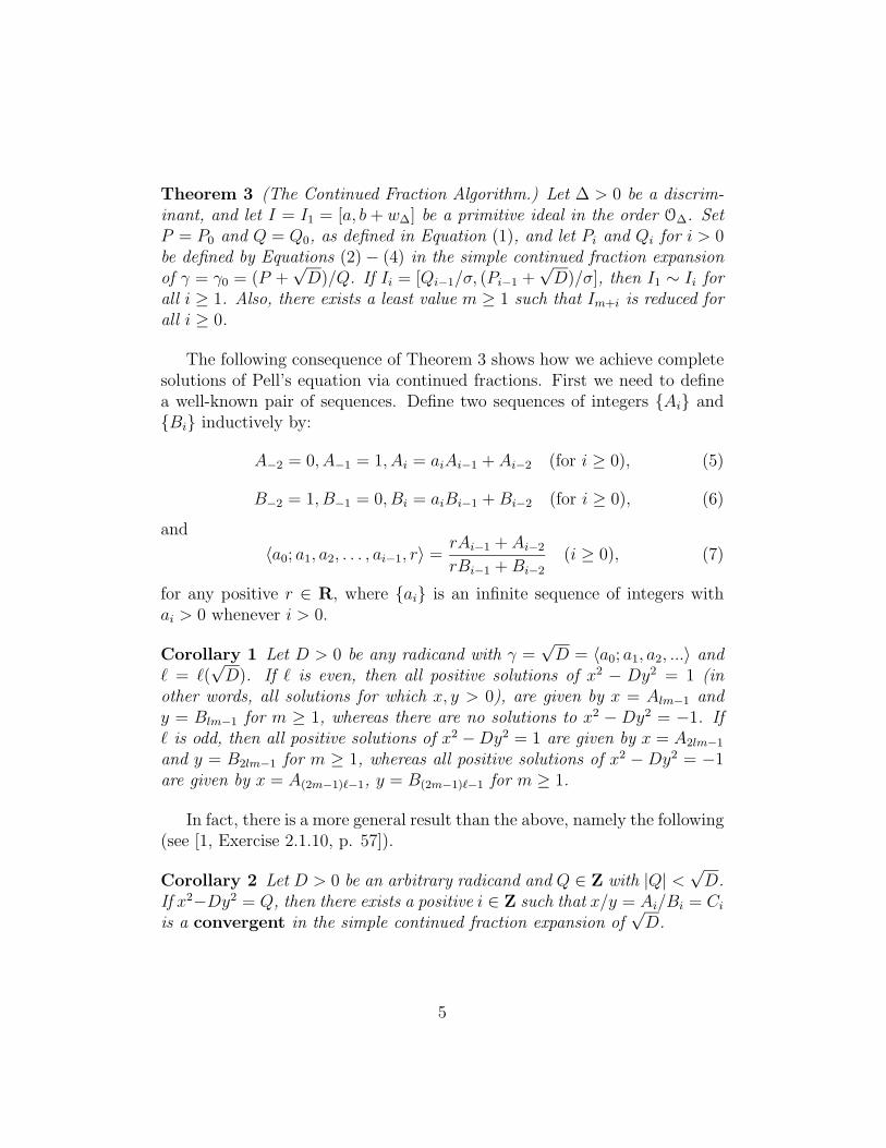
Theorem 3 (The Continued Fraction Algorithm.) Let ∆ > 0 be a discrim-inant, and let I = I1 = [a, b + w∆] be a primitive ideal in the order O∆. SetP = P0 and Q = Q0, as defined in Equation (1), and let Pi and Qi for i > 0be defined by Equations (2) − (4) in the simple continued fraction expansionof γ = γ0 = (P +

√D)/Q. If Ii = [Qi−1/σ, (Pi−1 +

√D)/σ], then I1 ∼ Ii for

all i ≥ 1. Also, there exists a least value m ≥ 1 such that Im+i is reduced forall i ≥ 0.

The following consequence of Theorem 3 shows how we achieve completesolutions of Pell’s equation via continued fractions. First we need to definea well-known pair of sequences. Define two sequences of integers {Ai} and{Bi} inductively by:

A−2 = 0, A−1 = 1, Ai = aiAi−1 + Ai−2 (for i ≥ 0), (5)

B−2 = 1, B−1 = 0, Bi = aiBi−1 + Bi−2 (for i ≥ 0), (6)

and

〈a0; a1, a2, . . . , ai−1, r〉 =rAi−1 + Ai−2

rBi−1 + Bi−2

(i ≥ 0), (7)

for any positive r ∈ R, where {ai} is an infinite sequence of integers withai > 0 whenever i > 0.

Corollary 1 Let D > 0 be any radicand with γ =√D = 〈a0; a1, a2, ...〉 and

' = '(√D). If ' is even, then all positive solutions of x2 − Dy2 = 1 (in

other words, all solutions for which x, y > 0), are given by x = Alm−1 andy = Blm−1 for m ≥ 1, whereas there are no solutions to x2 −Dy2 = −1. If' is odd, then all positive solutions of x2 −Dy2 = 1 are given by x = A2lm−1

and y = B2lm−1 for m ≥ 1, whereas all positive solutions of x2 −Dy2 = −1are given by x = A(2m−1)�−1, y = B(2m−1)�−1 for m ≥ 1.

In fact, there is a more general result than the above, namely the following(see [1, Exercise 2.1.10, p. 57]).

Corollary 2 Let D > 0 be an arbitrary radicand and Q ∈ Z with |Q| <√D.

If x2−Dy2 = Q, then there exists a positive i ∈ Z such that x/y = Ai/Bi = Ci

is a convergent in the simple continued fraction expansion of√D.

5

Remark 2 It is exactly Corollary 2 which Zhang [op.cit.] sought to gen-eralize. However, as he admitted in [4], his choices for those semi-simplecontinued fractions are not unique. In fact, therein, he seeks to achieve whathe calls minimal continued fractions, and leaves a conjecture [4, p.6] which isanswered by the theory which we develop in this paper since our choices areexplicit and unique.

This author found it difficult to apply the theory developed by Zhang sinceit is abstract, not explicit in terms of generating solutions, and for this au-thor at least, difficult to follow given the unusual approach which includesnone of the continued fraction algorithm or ideal theory. In other words, theinfrastructure was not employed in any fashion. We remedy this situation inthe next section where we give complete and explicit solutions of Equation (8)based upon the infrastructure and classical theory which we are delineating inthis section. Furthermore, Zhang’s work must be credited with inspiring thisauthor to develop the ideas presented in this paper.

In this paper, we will be concerned with solutions of the quadratic Dio-phantine equation

x2 −Dy2 = Q (8)

where Q ∈ Z is arbitrary, and D is any radicand.

Definition 1 If gcd(x, y) = 1 (x �= 0, y > 0) in equation (8), then we callα = x + y

√D a proper solution of that equation. Furthermore, if α =

x + y√D ∈ [1,

√D] with gcd(x, y) = 1 (x �= 0, y > 0), then α is called a

primitive element of [1,√D].

In the next section, we will show how proper solutions of Equation (8) areobtained from convergents of a more general principal cycle by making greateruse of the continued fraction algorithm.

From Theorem 3 , we get all reduced ideals equivalent to a given reducedideal I = [N(I), b + ω∆]. In other words, in the simple continued fractionexpansion of the quadratic irrational (b + ω∆)/a, where a = N(I), we have,for Pi and Qi as in Equations (1)-(4):

I = I1 = [Q0/σ, (P0 +√D)/σ] ∼ I2 = [Q1/σ, (P1 +

√D)/σ]

∼ ... ∼ Il = [Ql−1/σ, (Pl−1 +√D)/σ].

6

Finally, Il+1 = I1 = I for a complete cycle of reduced ideals equivalent toI of period length l(I) = l. Therefore, the (Pi +

√D)/Qi are the complete

quotients of (b + ω∆)/N(I) = γ, and the ai’s are the partial quotients of γ.Also, the Qi/σ’s represent the norms of all reduced ideals equivalent to I.Note that l = l(γ) = l(I) is the period length of the cycle of reducedideals equivalent to I, which, in turn, is the period length of the simplecontinued fraction expansion of the quadratic irrational γ.

If I is not reduced in the above, then we may still invoke Theorem 3.Any ideal may be chosen, whether or not it is reduced, and whether or notits norm is positive. If we take any ideal I in O∆, then we refer to theideals produced by the application of the continued fraction algorithm as acycle of ideals equivalent to I, which Theorem 3 tells us must be (eventually)purely periodic, as described above. For instance, the following illustratesthe process, and will be a motivator for results in the next section.

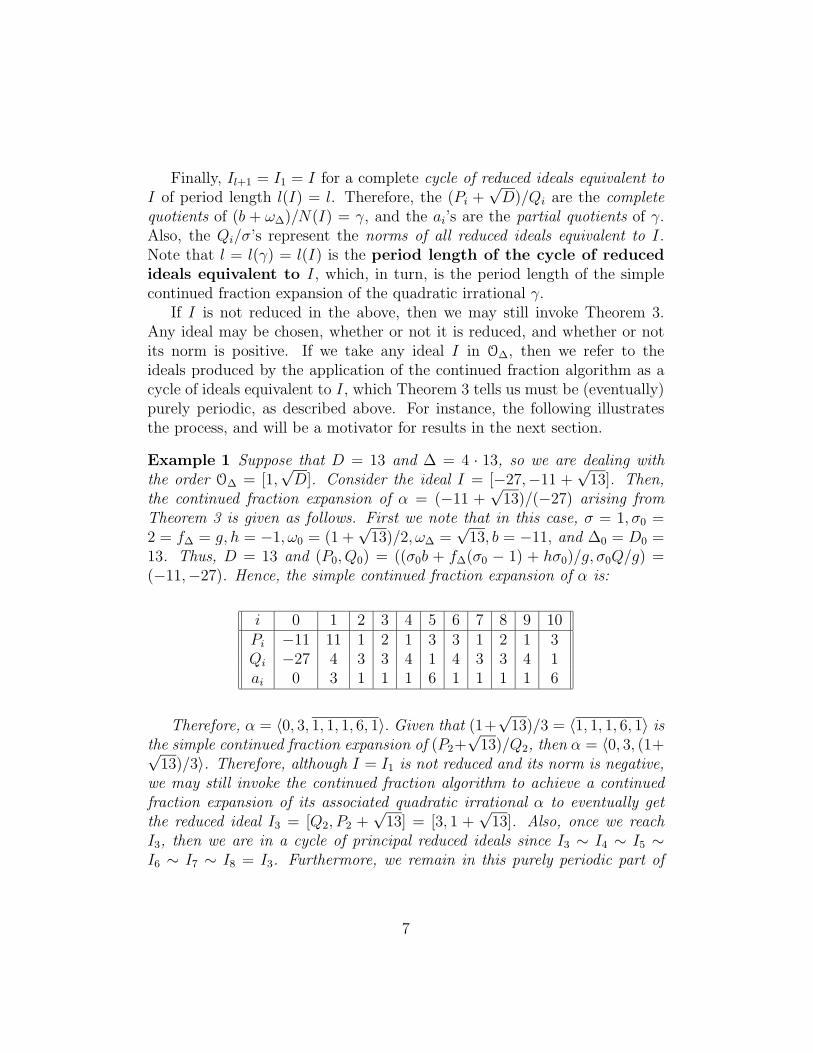
Example 1 Suppose that D = 13 and ∆ = 4 · 13, so we are dealing withthe order O∆ = [1,

√D]. Consider the ideal I = [−27,−11 +

√13]. Then,

the continued fraction expansion of α = (−11 +√

13)/(−27) arising fromTheorem 3 is given as follows. First we note that in this case, σ = 1, σ0 =2 = f∆ = g, h = −1, ω0 = (1 +

√13)/2, ω∆ =

√13, b = −11, and ∆0 = D0 =

13. Thus, D = 13 and (P0, Q0) = ((σ0b + f∆(σ0 − 1) + hσ0)/g, σ0Q/g) =(−11,−27). Hence, the simple continued fraction expansion of α is:

i 0 1 2 3 4 5 6 7 8 9 10Pi −11 11 1 2 1 3 3 1 2 1 3Qi −27 4 3 3 4 1 4 3 3 4 1ai 0 3 1 1 1 6 1 1 1 1 6

Therefore, α = 〈0, 3, 1, 1, 1, 6, 1〉. Given that (1+√

13)/3 = 〈1, 1, 1, 6, 1〉 isthe simple continued fraction expansion of (P2+

√13)/Q2, then α = 〈0, 3, (1+√

13)/3〉. Therefore, although I = I1 is not reduced and its norm is negative,we may still invoke the continued fraction algorithm to achieve a continuedfraction expansion of its associated quadratic irrational α to eventually getthe reduced ideal I3 = [Q2, P2 +

√13] = [3, 1 +

√13]. Also, once we reach

I3, then we are in a cycle of principal reduced ideals since I3 ∼ I4 ∼ I5 ∼I6 ∼ I7 ∼ I8 = I3. Furthermore, we remain in this purely periodic part of

7

the cycle of principal ideals after this point—ad infinitum.4

The process illustrated in Example 1 is of fundamental importance. The-orem 3 tells us that there always exists some minimal positive n ∈ Z suchthat In+i is reduced for all i ≥ 0. We therefore introduce a refinement of theterm for this integer, when Qn = 1, which will be part of our classificationdevice in the next section.

Definition 2 Let ∆ > 0 be a discriminant with radicand D. If I = I1 =[Q0/σ, (P0 +

√D)/σ] is a primitive, principal ideal in O∆, and the ideals Ii

are the ideals produced by the application of Theorem 3, then the least positiven ∈ Z such that Qn = 1 is called the principal reduction index of I.

Remark 3 Note that In+i is reduced for all i ∈ Z with i ≥ 0, (see [1,Theorem 2.1.2, pp. 44-47].) Also, observe that it is possible for In+1 =[Qn/σ, (Pn+

√D)/σ] to be reduced without γn = (Pn+

√D)/Qn being reduced.

For instance, I1 = [1,√D] = [1,

√D + �

√D�] is reduced, but γ0 =

√D is

not. However, whether or not γn is reduced, γn+i is reduced for all i ≥ 1 (see [1, Claim 4, pg. 45]).

In Example 1, the principal reduction index of I is n = 5 since Q5 = 1and I5+i is reduced for all i ≥ 1. Note that, the purely periodic part, initiatedby the principal reduction index, may not be the initial purely periodic partas determined by Theorem 3. For instance in Example 1, the purely periodicpart actually begins with I3 = [3, 1 +

√13]. However, we will be concerned

with that periodic part initiated by the principal reduction index since it isintimately linked to the solution of Equation (8).

Observe that, since [1, 3 +√

13] = [1,√

13], by Theorem 2, then we areessentially dealing with the continued fraction expansion of the principalsurd

√13. We will make this more explicit in the next section. Thus, the

principal reduction index is a basic tool which we will use in the next sectionto classify all solutions to Equation (8) via the continued fraction expansionof the principal surd. In general, if the ideal I = I1 = [N(I), b + ω∆] isitself already reduced, then the purely periodic part of the cycle begins with

4Also, witness that I4 = [Q3, P3 +√

13] = [3, 2 +√

13] = I ′3. We call i = 4 thepalindromic index. See [1, pp.188-198], where we develop the structure surrounding thepalindromy in ambiguous cycles.

8

I1, and this is the content of the above discussion about cycles of reducedideals from which we get l(I) = l(γ) where γ = (b + ω∆)/N(I). However,even in this case we have n > 0 if Q0 �= 1. The relationship between l(γ)and n when I is not reduced is illustrated by Example 1, wherein n = 5 andl(√D) = 5. Hence, I6 = [1, 3+

√13] begins the purely periodic part, initiated

by Qn = 1 (i.e. by the principal reduction index), of the simple continuedfraction expansion of α = (−11+

√13)/(−27). Since the following discussion

requires an understanding of the interplay of the fundamental units in variousrelated quadratic orders, and hence the Pell equation, we give the followingresults.

The next result dates back to Lagrange (see [1, Theorem 2.1.3, pp. 51-52]).

Theorem 4 Let I = [a, b + ω∆] be a reduced ideal, where ε∆ is the funda-mental unit of O∆. If Pi and Qi, for i = 1, 2, ..., l(I) = l, appear in the simplecontinued fraction expansion of (b + ω∆)/a, then

ε∆ =l∏

i=1

(Pi +√D)/Qi

andN(ε∆) = (−1)l.

We now describe the interplay between the fundamental units in twospecial orders, which has consequences for the solution of Pell’s equation aswell as more general equations. Since an arbitrary real quadratic order O∆

is always contained in the maximal order O∆0 , then ε∆ is a unit in O∆0 .Therefore, ε∆ = εu

∆0, where u is called the unit index of O∆ in O∆0 .

In particular, if O∆0 = [1, (1 +√D)/2] for D ≡ 1 (mod 4), then set

O∆ = [1,√D] where ∆ = 4∆0 = f 2

∆D = f 2∆∆0. In this case, either ε∆ = ε3∆0

or ε∆ = ε∆0 .5

5This follows from the general class number formula for real quadratic orders. See,for example [1 , footnote 1.5.9, pp. 25-26 ]. If f∆ > 1 is the conductor of an order O∆

with fundamental discriminant ∆0 and unit index u, then h∆ = h∆0ψ∆0(f∆)/u whereψ∆0(f∆) = f∆

∏(1 − (∆0/p)/p) with the product ranging over all the distinct primes

dividing f∆ and (∗/∗) denotes the Kronecker symbol. It is known that h∆ ≥ h∆0 . Indeed,h∆/h∆0 ∈ Z, but it is an open question as to when h∆ = h∆0 . In any case, u dividesψ∆0 . Thus, in our special case we deduce that h∆ = h∆0 when ∆ ≡ 1 (mod 8), andh∆ = 3h∆0/u when ∆ ≡ 5 (mod 8). In other words, either ε∆ = ε3∆0

or ε∆ = ε∆0 .

9

Now we review the process by which all of the proper solutions of Equation(8) emanate from its fundamental solutions which we now define.

Definition 3 If α = x + y√D is a proper solution of Equation (8), then

so are certain of its associates, namely those β ∈ O∆ (= [1,√D], not

necessarily maximal 6) for which there is a u ∈ U∆, u �= 1 with N(u) = 1such that β = uα. Thus, α and β are called a proper associated solutionsof Equation (8). These associated solutions7 form a class of solutions. Foreach such class we have an α0 = x0 + y0

√D with y0 > 0 being the smallest

value possible in its class. If −x0 + y0

√D is also in the class, then the class

is called ambiguous, and so in order to ensure a unique choice of α0, weassume that x0 > 0 in this case8. We call such a solution the fundamentalsolution of its class. Hence, all solutions of Equation (8) are given bycertain associates of the fundamental solutions in these (finitely many 9)classes.

Remark 4 An easy exercise shows that two solutions of Equation (8), α =x + y

√D and α1 = x1 + y1

√D, are in the same class if and only if both

(x1x− y1yD)/Q ∈ Z and (yx1 − xy1)/Q ∈ Z.

In the next section we will need to distinguish between two types ofassociates of a given solution of Equation (8). We do this as follows.

Definition 4 Suppose that α and β are proper associated solutions of Equa-tion (8). Then β is called a positive associate of α if β = εi

∆α where i ∈ Zis positive. If i < 0, then β is called a negative associate of α.10

6Here ∆ = 4D is a discriminant with radicand D, where D may be congruent to 1modulo 4, in which case σ0 = g = 2|f∆, and we are not dealing with the maximal orderin that situation. In any case σ = 1.

7As observed by Nagell [2, p. 205]. We also now see why the proper solutions ofDefinition 1 were chosen in that fashion, namely in order to coincide with Nagaell’s notionof solutions (as well as to avoid trivialities).

8In the next section we will develop a unique ideal associated with each proper solution,and therefore we will be able to link all of this to ideal theory (see Definition 5).

9See Nagell [2, Theorem 109, pp. 207-208]. Note that, if N(ε∆) = 1 (in other words,l(√D) is even by Theorem 4), then all associates of α0 are solutions of Equation (8). On

the other hand, if N(ε∆) = −1, then all associates of the form ε2i∆α0 for any i ∈ Z are

solutions of Equation (8).10Note that, if N(ε∆) = −1, then i must be even (see footnote 9).

10

Note that β is a positive associate of α if and only if α is a negativeassociate of β. Hence, the intersection of positive and negative associates ofa given solution is empty. In other words, a positive associate can never bea negative associate of a given solution of Equation (8).

For instance, we have the following.

Example 2 Consider the Diophantine equation

x2 − 13y2 = −27. (9)

A fundamental solution of it is α0 = −5+2√

13. Since the fundamental unitof O∆ = [1,

√13] is ε∆ = 18 + 5

√13, then all solutions in the class of α0 are

ε2n∆ α0, for n ∈ Z ( since N(ε∆) = −1). For instance, ε2∆α0 = 1435+398

√13.

Similarly, −α′0 = 5 + 2

√13 is a fundamental solution of the above equa-

tion, and so are all of its associates ε2n∆ (−α′

0), (n ∈ Z) . For example,(18 + 5

√13)2(5 + 2

√13) = 7925 + 2198

√13.

In the next section, we will show how these solutions and all others inthe various classes of solutions are convergents in a certain (not necessarilysimple) continued fraction expansion of

√13.

All of the above will be explained in a new and revealing way, using onlythe continued fraction algorithm.

2 Quadratic Diophantine Equations

Numerous symbols will be used and assumptions held throughout this sectionso we fix these in a sequence of conventions which we will state as the needarises, the first being as follows.

Convention 1 Throughout this section we assume that ∆ > 0 is a dis-criminant (not necessarily fundamental) with associated radicand D, andO∆ = [1,

√D] (not necessarily maximal). Furthermore we set l = l(

√D) =

l(√D + �

√D�) (see Remark 1, and footnote 6).

First we show how proper solutions of Diophantine equations are linkedto the existence of uniquely determined ideals.

11

Proposition 1 If α0 = x0+y0

√D ∈ O∆ is primitive with N(α0) = Q0, then

there exists a unique primitive element α = x + y√D ∈ O∆ such that

αα′0 = P0 +

√D,

with−|Q0|/2 < P0 ≤ |Q0|/2.

Also,x = (x0P0 + Dy0)/Q0,

andy = (x0 + y0P0)/Q0.

In this fashion, α determines a unique ideal I = [Q0, P0 +√D] corresponding

to α0.

Proof. Since gcd(x0, y0) = 1, then x0y1−y0x1 = 1 for some x1, y1 ∈ Z. In fact,for a fixed such solution, we may give the general solution by x = x1 + tx0,and y = y1 + ty0 for some parameter t ∈ Z. In other words, x0y − y0x = 1.Thus, if α = x + y

√D, then

αα′0 = x0x− y0yD + (x0y − y0x)

√D = P0 +

√D,

where P0 = x0x − y0yD = x0x1 − y0y1D − tQ0. We may therefore chooseP0 uniquely such that −|Q0|/2 < P0 ≤ |Q0|/2, and N(αα′

0) = N(α)N(α′0).

Hence, we may form the ideal11

I = [Q0, P0 +√D].

SinceP0 = x0x− y0yD, (10)

and

1 = x0y − y0x, (11)

then, adding y0 times Equation (10) to x0 times Equation (11) yields:

x0 + y0P0 = x20y − y2

0yD = yQ0.

11Observe that, even if the ideal is ambiguous, (in which case I = I ′ = [Q0,−P0 +√D]),

P0 is unique since we are restricted to the choice of P0 = |Q0|/2 in this case by the strictinequality −|Q0|/2 < P0.

12

Therefore, y = (x0 + y0P0)/Q0. Plugging this value of y into Equation (11),we get x = (x0P0 + Dy0)/Q0. ✷

Since α0 is a proper solution of Equation (8) with Q = Q0, then wenecessarily have the following.

Corollary 3 Iα0∼ 1.

Proof. Since Iα0= (α′

0)[Q0/α′0, α] ∼ [α0, α], then Iα0

∼ [α0, α]. However,yα0 − y0α = 1, so [α0, α] ∼ 1. Hence, Iα0

∼ 1. In fact, Iα0= (α′

0), since[α0, α] = (1) = O∆. ✷

Proposition 1 motivates the following definition.

Definition 5 If α0 ∈ O∆ is primitive, then the unique ideal correspond-ing to α0 is given by Iα0 = [Q0, P0 +

√D], as determined by Proposition

1.

This unique ideal, associated with a given solution of Equation (8), pro-vides the anchor for an application of the continued fraction algorithm, The-orem 3, and so will provide the genesis for the complete solutions of Equation(8) via continued fractions. Since we will be discussing several different con-tinued fraction expansions of various quadratic irrationals, we need to setsome notation. We do this in the following.

Convention 2 In what follows, Iα0 = [Q0, P0 +√D] shall denote the ideal

established in Definition 5, and it will be assumed throughout to have prin-cipal reduction index n. Furthermore, it will be understood that the symbolsAi, Bi, Pi, Qi, ai, n, etc. will denote those values arising from the simple con-tinued fraction expansion of (P0 +

√D)/Q0. Also, we set γi = (Pi +

√D)/Qi

(i ≥ 0) in that continued fraction expansion. Moreover, we use the tilde no-tation for the values arising from the simple continued fraction expansion ofPn +

√D = γ0. Thus, we have for example Ai, Bi, Pi, Qi, ai etc. Finally, we

use the symbols Ai, Bi, Pi, Qi, ai, etc. for the values arising from the simplecontinued fraction expansion of −α′

0 = (−P0+√D)/Q0, in other words, from

the unique ideal I−α′0corresponding to −α′

0, which we will assume throughoutto have principal reduction index n.

13

Proposition 1 is a generalization of the result [6, Lemma 3, p. 194], whichactually masks the connection between the ideal theory and the continuedfraction algorithm called the infrastructure by Dan Shanks (see [1, Chapters7-8, pp. 223-266]). The following example will motivate our further devel-opment of this connection. Furthermore, this example begins our trek intolearning how to use the continued fraction algorithm, Theorem 3, to get acontinued fraction expansion of

√D in which all solutions of Equation (8)

will be convergents.

Example 3 If we look back at Examples (1) − (2), we see that α0 = −5 +2√

13 is a proper solution of Equation (9). The unique ideal correspondingto α0 is given by Iα0

= [−27,−11 +√

13] (where the α of Proposition 1 is

given by α = x + y√

13 = −3 +√

13). In Example 1 we displayed the simplecontinued fraction expansion of (−11 +

√13)/(−27), where the principal re-

duction index is n = 5. Furthermore, this means that (−11 +√

13)/(−27) =〈0, 3, 1, 1, 1, 6, 1, 1, 1, 1〉 = 〈0, 3, 1, 1, 1, 3 +

√13〉. By Equation (7),

(−11 +√

13)/(−27) =A4(3 +

√13) + A3

B4(3 +√

13) + B3

.

Hence,√

13 = −27A4(3 +

√13) + A3

B4(3 +√

13) + B3

+ 11 =

(−27A4 + 11B4)(3 +√

13) − 27A3 + 11B3

B4(3 +√

13) + B3

.

This shows the relationship between the continued fraction expansion of√13 and that of α0.

Example 3 motivates the following definition of some well-known se-quences related to Equations (5)-(6) (see [1, Exercise 2.1.2, pp. 54-56]).

Definition 6 Given a quadratic irrational α = (P +√D)/Q ∈ O∆ with

α = 〈a0; a1, a2, . . .〉, set

Gi−1 = Q0Ai−1 − P0Bi−1 (i ≥ −1). (12)

ThenN [(Gi−1 + Bi−1

√D)] = (−1)iQiQ0 (i ≥ 0), (13)

14

where the sequences {Ai} and {Bi} arise from the continued fraction expan-sion of α via Equations (5) − (6). Also, if δm−1 =

∏mi=1(Pi +

√D)/Qi, then

δm−1 = (Gm−1 + Bm−1

√D)/Qm. (14)

Also, we have:

Gi−1 = PiBi−1 + QiBi−2 (i ≥ 0), (15)

DBi−1 = PiGi−1 + QiGi−2 (i ≥ 0), (16)

andGi = aiGi−1 + Gi−2 (i ≥ 0). (17)

Now we may examine Example 3 in light of the above.

Example 4 Notice that in Example 3, Q0 = −27, P0 = −11, and n =l(√

13) = l = 5, so

√13 =

Glm+n−1(3 +√

13) + Glm+n−2

Blm+n−2(3 +√

13) + Blm+n−2

(m ≥ 0).

Since Qlm+n = 1, and Equation (13) tells us that

N(Glm+n−1 + Blm+n−1

√13) = (−1)lm+n(−27),

then we get a solution of Equation (9) exactly when lm + n is even, i.e.when m is odd. The first such value is therefore lm + n − 1 = 9, andG9 + B9

√13 = 1435 + 398

√13. Now, if we look back to Example 2, we see

that ε2∆α0 = 1435 + 398√

13, the first positive associate of α0. In fact, thepositive associates of α0 are exactly the G9+10j +B9+10j

√D for all j ≥ 0. We

will establish this phenomenon as a general fact below.

In order to classify all solutions of Equation (8) via convergents in con-tinued fraction expansions, we first need to establish a preliminary fact. Werefer the reader to Convention 2 for notation.

The following links Definition 6 with fundamental units. This will provideus with a means of linking up the continued fraction expansion of

√D with

that of (P0 +√D)/Q0.

15

Proposition 2 For any positive m ∈ Z,

εm∆ = Glm−1 + Blm−1

√D,

(and so ε−m∆ = Glm−1 − Blm−1

√D).

Proof. See [1, Theorem 2.1.3, p. 51] and [1, Exercise 2.1.2, pp. 54-56]. ✷

Using Proposition 2, we can now show that certain of the δi described inDefinition 6 are always associates of α0 for a given fundamental solution α0.

Proposition 3 If α0 is a proper solution of Equation (8) which the funda-mental solution in its class, k(m) = lm+n−1 and k(m) = lm+n−1 (m ∈ Z)(in the negative conjugate), then:

(1) If δk(m) = Gk(m) + Bk(m)

√D �= α0, then δk(m) is a positive associate of

α0 for any non-negative m ∈ Z such that k(m) is odd.

(2) If δk(m) = Gk(m) + Bk(m)

√D �= α0, then −δ′

k(m)is a negative associate of

α0 for any non-negative m ∈ Z such that k(m) is odd.

Proof. First we prove (1). To establish that δk(m) is a solution associatedwith α0, we invoke Remark 4. Since k(m) is odd and Qk(m)+1 = 1 for all non-negative m ∈ Z, then δk(m) is a proper solution of Equation (8) via Equation(13). Thus, we need only show that both

(x0Gk(m) − y0Bk(m)D)/Q0 = E ∈ Z,

and(y0Gk(m) − x0Bk(m))/Q0 = F ∈ Z.

By Proposition 1,

x0P0 = Q0(x0P0 + Dy0)/Q0 − y0D = Q0x− y0D.

Therefore, multiplying both sides by Bk(m) and using Equation (12), we get:

x0Ak(m)Q0 − x0Gk(m) = Q0xBk(m) − y0DBk(m),

so by rearranging,

(x0Gk(m) − y0DBk(m))/Q0 = x0Ak(m) − xBk(m).

16

In other words, E = x0Ak(m) − xBk(m) ∈ Z.Similarly, by Proposition 1:

y0P0Bk(m) = yQ0Bk(m) − x0Bk(m).

Again, using Equation (12):

y0Ak(m)Q0 − y0Gk(m) = yQ0Bk(m) − x0Bk(m).

After rearranging we get:

F = (y0Gk(m) − x0Bk(m))/Q0 = y0Ak(m) − yBk(m) ∈ Z.

We have demonstrated that all of the δk(m) are associates of α0. We nowshow that these associates must be positive. Suppose that ε−i

∆ α0 = δk(m)

for some i > 0 (where i is even if N(ε∆) = −1; see footnote 9), and somenon-negative m ∈ Z.

Since ε−i∆ = Gil−1 − Bil−1

√D by Proposition 2 then,

Gk(m) = x0Gil−1 − y0Bil−1D, (18)

andBk(m) = y0Gil−1 − x0Bil−1. (19)

Multiplying Equation (18) by Bil−1 and adding Gil−1 times Equation (19),we get:

y0 = Gil−1Bk(m) + Bil−1Gk(m).

However,Bj ≥ Bj−1 ≥ 0, Gj > Gj−1 > 0

for all j ≥ 0 and Bk(m) > 0, Gk(m) > 0 for all k(m) ≥ 0,( for example see [1,Exercise 2.1.2(g), pp. 55]). Hence,

y0 > Gl(i−1)−1Bk(m) + Bl(i−1)−1Gk(m) = v > 0.

However, if

u = Gl(i−1)−1Gk(m) + Bl(i−1)−1Bk(m)D,

thenε−1∆ α0 = εi−1

∆ δk(m) = u + v√D

17

is an associate of α0. Thus, by the minimality of y0, v ≥ y0, a contradiction.This secures (1).

By (1), δk(m) is a positive associate of −α′0, so there exists a positive i ∈ Z

such that εi∆(−α′

0) = δk(m). Hence, −δ′k(m)

is a negative associate of α0. This

secures (2) and so the entire result. ✷

Proposition 3 showed that all δk(m) are positive associates of α0. Now weshow that the δk(m) are all of the positive associates of the minimum δk(m)

possible for which k(m) is odd, together with the related result for negativeassociated solutions, and that α0 is either γk(m0) or −γ′

k(m0). This guarantees

that we have a means of generating all solutions of Equation 8.

Theorem 5 Suppose that α0 is a proper solution of Equation (8), such thatα0 is fundamental in its class, k(m) = lm + n− 1, and k(m) = lm + n− 1,for any non-negative m ∈ Z. Then each of the following must hold.

(1) If m = m0 is the least non-negative integer such that k(m) is odd, then allpositive associates of δk(m0) = Gk(m0) + Bk(m0)

√D are given by δk(m) =

Gk(m) + Bk(m)

√D, for all m > m0 such that k(m) is odd.

(2) All negative associates of δk(m0) are given by −δ′k(m)

= −Gk(m)+Bk(m)

√D

for all m ≥ m0 such that k(m) is odd, where m = m0 is the least non-negative integer such that k(m) is odd.

(3) If α0 �= δk(m0), then α0 = −δ′k(m0)

.

Proof. First we prove (1), which we treat by cases.

Case 1. Assume that n is even, and l is odd.

In this case m0 = 0. Thus, we wish to show that

εm∆δn−1 = δk(m)

for all even m > 0.Suppose that ε−m

∆ δk(m) = u + v√D. Then by Proposition 2,

ε−m∆ = Glm−1 − Blm−1

√D,

for all positive m ∈ Z. Thus:

18

u = Glm−1Gk(m) − Blm−1Bk(m)D, (20)

andv = Glm−1Bk(m) − Blm−1Gk(m). (21)

First, we concentrate upon showing that v = Bn−1. From Equation (15),together with the facts that Plm = Plm+n = �

√D�,12 and Qlm = 1 = Qk(m)+1

for all m > 0, Equation (21) becomes:

v = (�√D�Blm−1 + Blm−2)Bk(m) − Blm−1(�

√D�Bk(m) −Bk(m)−1),

which simplifies to:

v = Blm−2Bk(m) − Blm−1Bk(m)−1. (22)

From Equation (6), Equation (22) becomes:

v = Blm−2(ak(m)Bk(m)−1 + Bk(m)−2) − (alm−1Blm−2 + Blm−3)Bk(m)−1,

which, by the fact that alm−i = alm+n−i = ak(m)−i+1 for all positive i ≤ lmand even m > 0, simplifies to:

v = Blm−2Bk(m)−2 − Blm−3Bk(m)−1. (23)

Again, using the aforementioned facts, we get that Equation (23) be-comes:

v = (alm−2Blm−3 + Blm−4)Bk(m)−2 − Blm−3(ak(m)−1Bk(m)−2 + Bk(m)−3)

= Blm−4Bk(m)−2 − Blm−3Bk(m)−3.

Continuing in this fashion, we get, for any positive i ≤ lm/2+1 and evenm > 0, that:

v = Blm−2iBk(m)−2i+2 − Blm−2i+1Bk(m)−2i+1.

12In order to see that Plm+n = �D� for m > 0, we invoke [1, Theorem 2.1.2, Claims3-4, p.45] to get that δlm+n = δl+n = Pl+n +

√D is reduced for all m ≥ 1. Therefore, by

Remark 1, −1 < Pl+n −√D < 0, i.e. Pl+n = �D�.

19

In particular, if i = lm/2 + 1, then

v = B−2Bn−1 − B−1Bn−2 = Bn−1.

To get that u = Gn−1, we use similar facts and reasoning. First we note,that from Equations (15)-(16), Equation (20) becomes (for m > 0 even):

u = Glm−1(�√D�Bk(m) + Bk(m)−1) − (�

√D�Glm−1 + Glm−2)Bk(m),

which simplifies to:

u = Glm−1Bk(m)−1 − Glm−2Bk(m). (24)

Using Equations (6) and (17), we get that Equation (24) becomes

u = (alm−1Glm−2 + Glm−3)Bk(m)−1 − Glm−2(ak(m)Bk(m)−1 + Bk(m)−2),

which simplifies to

u = Glm−3Bk(m)−1 − Glm−2Bk(m)−2.

Again, using Equations (6) and (17), we get that this becomes:

u = Glm−3Bk(m)−3 − Glm−4Bk(m)−2.

Continuing in this fashion, we get that, for any positive i ≤ lm/2, andodd m > 0,

u = Glm−2i+1Bk(m)+1−2i − Glm−2iBk(m)−2i+2. (25)

In particular, for i = lm/2 + 1,

u = G−1Bn−2 − G−2Bn−1 = Bn−2 + Bn−1Pn = Gn−1,

with the latter coming from Equation (15), since G−2 = −P0 = −Pn andG−1 = Q0 = 1 = Qn.

This establishes Case 1.

Case 2. n is odd and l is odd.

In this case m0 = 1, so we seek to determine the positive associates ofδk(m0) = δl+n−1 = Gl+n−1 + Bl+n−1

√D. These will now be shown to be the

20

ε2t∆δl+n−1 = δk(2t+1) for all positive t ∈ Z. We analyze ε−2t

∆ δk(2t+1) = u+ v√D,

as in Case 1 to get:

v = B2lt−2iBk(2t+1)−2i+2 − B2t−2i+1Bk(2t+1)−2i+1,

for all positive i ≤ lt+ 1, and all positive t ∈ Z. In particular, for i = lt+ 1,we get:

v = B−2Bl+n−1 − B−1Bl+n−2 = Bl+n−1.

Similarly, we analyze as in Case 1 to get:

u = Bk(2t+1)−2i+1G2lt−2i+1 −Bk(2t+1)−2i+2G2lt−2i,

for any positive i ≤ lt + 1 and any t > 0. In particular, for i = lt + 1:

u = Bl+n−2G−1 −Bl+n−1G−2 = Bl+n−2 + PnBl+n−1.

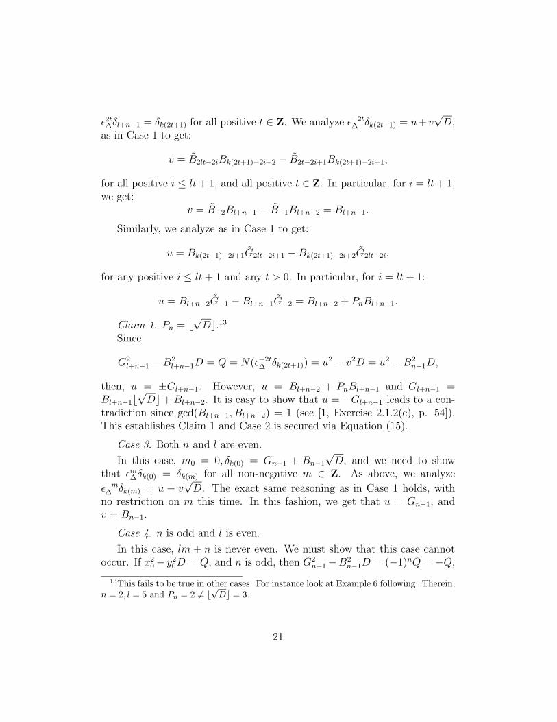
Claim 1. Pn = �√D�.13

Since

G2l+n−1 −B2

l+n−1D = Q = N(ε−2t∆ δk(2t+1)) = u2 − v2D = u2 −B2

n−1D,

then, u = ±Gl+n−1. However, u = Bl+n−2 + PnBl+n−1 and Gl+n−1 =Bl+n−1�

√D� + Bl+n−2. It is easy to show that u = −Gl+n−1 leads to a con-

tradiction since gcd(Bl+n−1, Bl+n−2) = 1 (see [1, Exercise 2.1.2(c), p. 54]).This establishes Claim 1 and Case 2 is secured via Equation (15).

Case 3. Both n and l are even.

In this case, m0 = 0, δk(0) = Gn−1 + Bn−1

√D, and we need to show

that εm∆δk(0) = δk(m) for all non-negative m ∈ Z. As above, we analyze

ε−m∆ δk(m) = u + v

√D. The exact same reasoning as in Case 1 holds, with

no restriction on m this time. In this fashion, we get that u = Gn−1, andv = Bn−1.

Case 4. n is odd and l is even.

In this case, lm + n is never even. We must show that this case cannotoccur. If x2

0 − y20D = Q, and n is odd, then G2

n−1 −B2n−1D = (−1)nQ = −Q,

13This fails to be true in other cases. For instance look at Example 6 following. Therein,n = 2, l = 5 and Pn = 2 �= �

√D� = 3.

21

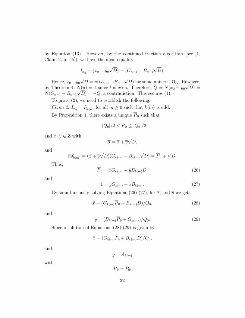
by Equation (13). However, by the continued fraction algorithm (see [1,Claim 2, p. 45]), we have the ideal equality:

Iα0= (x0 − y0

√D) = (Gn−1 −Bn−1

√D).

Hence, x0−y0

√D = u(Gn−1−Bn−1

√D) for some unit u ∈ O∆. However,

by Theorem 4, N(u) = 1 since l is even. Therefore, Q = N(x0 − y0

√D) =

N(Gn−1 −Bn−1

√D) = −Q, a contradiction. This secures (1).

To prove (2), we need to establish the following.

Claim 2. Iα0= Iδk(m)

for all m ≥ 0 such that k(m) is odd.

By Proposition 1, there exists a unique P 0 such that

−|Q0|/2 < P 0 ≤ |Q0|/2

and x, y ∈ Z withα = x + y

√D,

andαδ′k(m) = (x + y

√D)(Gk(m) −Bk(m)

√D) = P 0 +

√D.

Thus,P 0 = xGk(m) − yBk(m)D, (26)

and1 = yGk(m) − xBk(m). (27)

By simultaneously solving Equations (26)-(27), for x, and y we get:

x = (Gk(m)P 0 + Bk(m)D)/Q0, (28)

andy = (Bk(m)P 0 + Gk(m))/Q0. (29)

Since a solution of Equations (28)-(29) is given by

x = (Gk(m)P0 + Bk(m)D)/Q0,

andy = Ak(m)

withP 0 = P0,

22

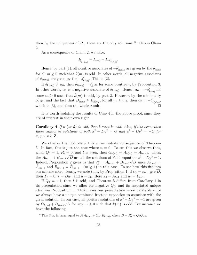
then by the uniqueness of P 0, these are the only solutions.14 This is Claim2.

As a consequence of Claim 2, we have:

Iδk(m0)= I−α′

0= I−δ′

k(m0).

Hence, by part (1), all positive associates of −δ′k(m0) are given by the δk(m)

for all m ≥ 0 such that k(m) is odd. In other words, all negative associatesof δk(m0) are given by the −δ′

k(m). This is (2).

If δk(m0) �= α0, then δk(m0) = εi∆α0 for some positive i, by Proposition 3.

In other words, α0 is a negative associate of δk(m0). Hence, α0 = −δ′k(m)

for

some m ≥ 0 such that k(m) is odd, by part 2. However, by the minimalityof y0, and the fact that Bk(m) ≥ Bk(m0) for all m ≥ m0, then α0 = −δ′

k(m0),

which is (3), and thus the whole result. ✷

It is worth isolating the results of Case 4 in the above proof, since theyare of interest in their own right.

Corollary 4 If n (or n) is odd, then l must be odd. Also, if l is even, thenthere cannot be solutions of both x2 − Dy2 = Q and u2 − Dv2 = −Q forx, y, u, v ∈ Z.

We observe that Corollary 1 is an immediate consequence of Theorem5. In fact, this is just the case where n = 0. To see this we observe that,when Q0 = 1, P0 = 0, and l is even, then Gk(m) = Ak(m) = Alm−1. Thus,

the Alm−1 + Blm−1

√D are all the solutions of Pell’s equation x2 −Dy2 = 1.

Indeed, Proposition 2 gives us that εm∆ = Alm−1 + Blm−1

√D since Alm−1 =

Alm−1 and Blm−1 = Blm−1 (m ≥ 1) in this case. To see how this fits intoour scheme more clearly, we note that, by Proposition 1, if ε∆ = x0 + y0

√D,

then P0 = 0, x = Dy0, and y = x0. Here x0 = Al−1 and y0 = Bl−1.If Q0 = −1, then l is odd, and Theorem 5 differs from Corollary 1 in

its presentation since we allow for negative Q0, and its associated uniqueideal via Proposition 1. This makes our presentation more palatable sincewe always have a unique continued fraction expansion to associate with thegiven solution. In our case, all positive solutions of x2 −Dy2 = −1 are givenby Gk(m) + Bk(m)

√D for any m ≥ 0 such that k(m) is odd. For instance we

have the following.

14This x is, in turn, equal to P0Ak(m) +Q−1Bk(m), where D = P 20 +Q0Q−1.

23

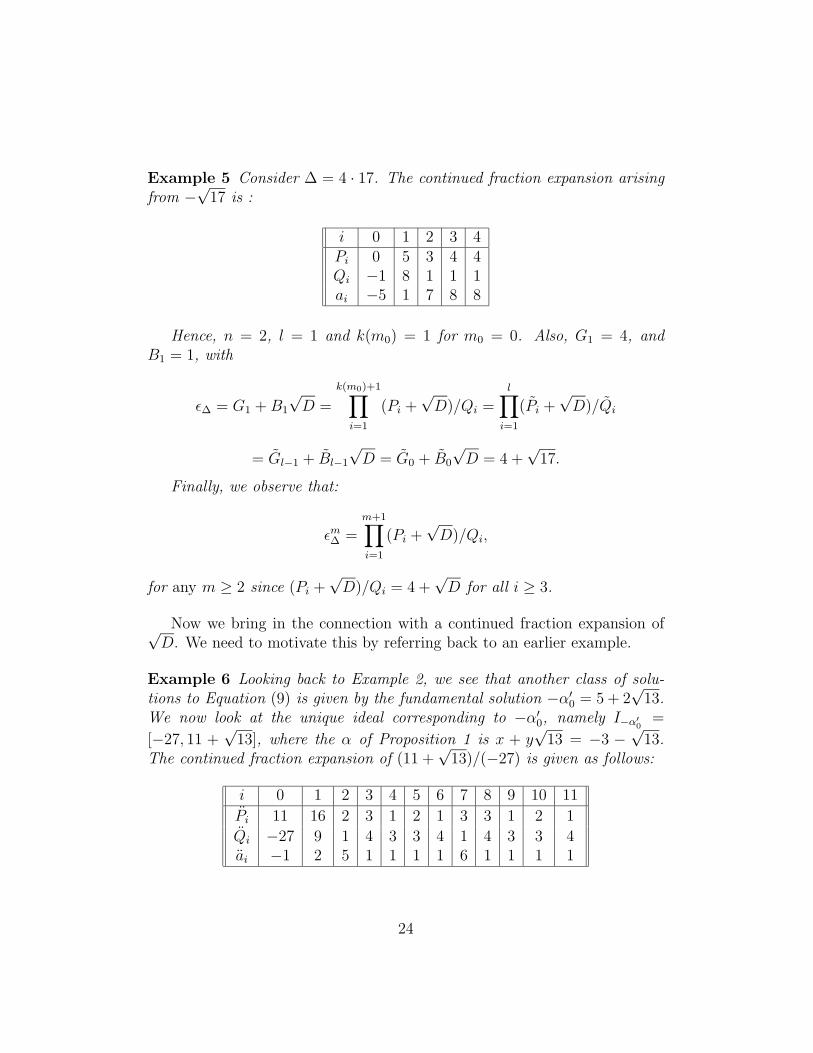
Example 5 Consider ∆ = 4 · 17. The continued fraction expansion arisingfrom −

√17 is :

i 0 1 2 3 4Pi 0 5 3 4 4Qi −1 8 1 1 1ai −5 1 7 8 8

Hence, n = 2, l = 1 and k(m0) = 1 for m0 = 0. Also, G1 = 4, andB1 = 1, with

ε∆ = G1 + B1

√D =

k(m0)+1∏i=1

(Pi +√D)/Qi =

l∏i=1

(Pi +√D)/Qi

= Gl−1 + Bl−1

√D = G0 + B0

√D = 4 +

√17.

Finally, we observe that:

εm∆ =

m+1∏i=1

(Pi +√D)/Qi,

for any m ≥ 2 since (Pi +√D)/Qi = 4 +

√D for all i ≥ 3.

Now we bring in the connection with a continued fraction expansion of√D. We need to motivate this by referring back to an earlier example.

Example 6 Looking back to Example 2, we see that another class of solu-tions to Equation (9) is given by the fundamental solution −α′

0 = 5 + 2√

13.We now look at the unique ideal corresponding to −α′

0, namely I−α′0

=

[−27, 11 +√

13], where the α of Proposition 1 is x + y√

13 = −3 −√

13.The continued fraction expansion of (11 +

√13)/(−27) is given as follows:

i 0 1 2 3 4 5 6 7 8 9 10 11

Pi 11 16 2 3 1 2 1 3 3 1 2 1

Qi −27 9 1 4 3 3 4 1 4 3 3 4ai −1 2 5 1 1 1 1 6 1 1 1 1

24

Notice that n = 2 for I−α′0

and −α′0 = G1 + B1

√D = 5 + 2

√13 = δk(m0)

since m0 = 0. Also, α0 = −δ′1 = −G1+B1

√D = −5+2

√13, since α0 �= δk(m)

for any m ≥ 0. In fact, δk(m0) = G9 +B9

√D = 1435 + 398

√13 = ε2∆α0 since

n = 5 for Iα0, thereby making k(m0) = lm0 + n − 1 = 5 · 1 + 5 − 1 = 9 the

minimum value for k(m) to be odd. The next positive associate of α0 is:

δ19 = G19 + B19

√D = 1862635 + 516602

√13 = ε2∆δk(m0) = ε4∆α0.

Thus we see that all positive associates of α0 are the δk(m+1) = Gk(m+1) +

Bk(m+1)

√13 = εm

∆α0 for all even m > 0. This is case 2 of Theorem 5.

Similarly, by Theorem 5, the −δ′k(m)

are negative associates of α0, and

by Theorem 5 all positive associates of −α′0 are the δk(m) for all m such

that k(m) = 5m + 1 is odd, so m is even. The first positive associate of−α′

0 = δk(m0) is ε2∆(−α′0) = G11 + B11

√13 = δk(2) = 7925 + 2198

√13. In

general, εm∆(−α′

0) = δk(m), so ε−m∆ α0 = −δ′

k(m)for any even m > 0. Therefore,

we have all of the negative associates of α0 in this fashion. The first occursfor m = 2, namely, ε−2

∆ α0 = −7925 + 2198√

13.The only other possible fundamental solution of Equation (9) is 12+3

√13.

However, this is not a proper solution. Hence, all proper solutions of x2 −13y2 = −27 are given by total of the ±Gk(m) + Bk(m)

√D for all m ≥ 0 such

that k(m) is odd, and the ±Gk(m) + Bk(m)

√D for all m ≥ 0 such that k(m)

is odd.

Example 6 suggests the following which is immediate from Theorem 5.

Theorem 6 All proper solutions of Equation (8) are given by the values±Gk(m) + Bk(m)

√D for all m ≥ 0 such that k(m) is odd, and the ±Gk(m) +

Bk(m)

√D for all m ≥ 0 such that k(m) is odd, as we allow the α0 to range

over all fundamental proper solutions of Equation (8) .

Now that we have all solutions of Equation (8) via the infrastructure, weexplain what is behind the work of Zhang [4]-[6] wherein solutions are listedas convergents in a semi-simple continued fraction expansion of

√D.

Lemma 1 Suppose that α0 = x0 + y0

√D ∈ O∆ is a primitive element such

that Iα0 = [Q0, P0 +√D], and n + lm ≥ 1. If γ0 = (P0 +

√D)/Q0 =

〈a0; a1, . . .〉, then for any non-negative m ∈ Z,√D = 〈−Plm+n;−alm+n−1,−an+lm−2, . . . ,−a1,−a0 + γ0〉.

25

Furthermore, Plm+n = �√D� if m > 0.15

Proof. Since γi+1 = 1/(−ai + γi) (see the proof of [1, Theorem 2.1.1, pp.42-43], for instance), and Qlm+n = 1 , then γlm+n = Plm+n +

√D. Therefore,

√D = γlm+n − Plm+n = −Plm+n +

1

−alm+n−1 + γlm+n−1

=

−Plm+n +1

−alm+n−1 +1

−alm+n−2 + γlm+n−2

= · · ·

Hence,

√D = 〈−Plm+n;−alm+n−1,−alm+n−2, . . . ,−a1,−a0 + γ0〉.

To see that Plm+n = �D� for m > 0, we invoke footnote 12. This com-pletes the proof. ✷

Lemma 1 motivates the following.

Definition 7 The continued fraction expansion of√D (for lm + n ≥ 1),

in Lemma 1 is called the (lm+n)th continued fraction expansion of√D arising from Iα0

, which is uniquely determined by l, m, and n sincethe simple continued fraction expansion of γ0, upon which this expansion isbased, is uniquely determined by Theorem 3.

At this juncture, we must ensure that we can distinguish between the val-ues arising from Equations (1)-(7) , in comparisons of the continued fractionexpansions of

√D via Definition 7, and that of others defined above. We

need to set some notation. We do this as follows.

Convention 3 We use the hat notation to denote values arising from thecontinued fraction expansion of

√D as given in Definition 7, such as Ai, and

δi.

With this notation in place we have the following result from Lemma 1.

15If γn is reduced, then Pn = �√D� as well. However, as observed in Remark 3, it is

possible for In+1 to be reduced without γn being reduced (see Example 6 for instance) .

26

Corollary 5 For the (lm + n)th continued fraction expansion of√D given

in Lemma 1, we have Pi = −Plm+n+1−i for 1 ≤ i ≤ lm + n with P0 = 0, andQi = Qlm+n−i for 1 ≤ i ≤ lm + n with Q0 = 1.

Proof. Since Q0 = 1 = Qlm+n, and a0 = P1 = −Plm+n, then

D = P 21 + Q1 = P 2

lm+n + Qlm+n−1,

so Q1 = Qlm+n−1. As induction hypothesis, assume Pi = −Plm+n+1−i andQi = Qlm+n−i whenever 1 ≤ i < lm + n. Since we also have established thatai = −alm+n−i, whenever 1 ≤ i < lm + n, then

Plm+n = alm+n−1Qlm+n−1 − Plm+n−1 = −a1Q1 + P2 = −P1.

Also,Qlm+n = (D − P 2

lm+n)/Qlm+n−1 = (D − P 21 )/Q1 = Q0.

This completes the proof. ✷

We observe that Equations (5)-(6) hold for the Ai and Bi despite the factthat the partial quotients are negative. We must caution the reader thatalthough the continued fraction expansion of

√D as given in Definition 7

satisfies Equations (1)-(3) and (5)-(7), it does not respect Equation (4). Thereason is that the values of the partial quotients ai are positive for all i ≥ 1in the simple continued fraction expansion of any quadratic irrational. Thisis implicit in Theorem 3. In point of fact, the use of the floor of an integer asthe definition of the partial quotient in Equation (4) is precisely what keepsthose partial quotients positive (for all i ≥ 1) in the simple continued fractionexpansion of a given quadratic irrational. However, our continued fractionexpansion of

√D, as given in Definition 7, has negative partial quotients.

Thus, the equation ai = (Pi+1 + Pi)/Qi is the one which applies in this case.The following illustrates this process.

Example 7 By Lemma 1, we get that√

13 = 〈−3;−1,−1,−1,−3, (−11 +√

13)/(−27)〉.The corresponding table is :

i 0 1 2 3 4 5 6 7 8 9 10 11 12 13 14 15

Pi 0 −3 −1 −2 −1 −11 11 1 2 1 3 3 1 2 1 3

Qi 1 4 3 3 4 −27 4 3 3 4 1 4 3 3 4 1ai −3 −1 −1 −1 −3 0 3 1 1 1 6 1 1 1 1 6

27

In the above table, columns 5-15 are given by Equations (1) − (4), as inExample 1. However, in columns 0-4 , Equation (4) fails. Instead we useai = (Pi+1 + Pi)/Qi, as determined by Equation (3).

The above motivates the following criterion.

Lemma 2 Suppose that α0 = x0 + y0

√D ∈ O∆ is a primitive element, and

k(m) = lm + n− 1 for any non-negative m ∈ Z such that k(m) is odd, thenthe following are equivalent.

(1) α0 is a proper solution of Equation (8).

(2) Q = Q0 = Qk(m)+1.

(3) A2k(m) − B2

k(m)D = Q = Q0.

(4) G2k(m) −B2

k(m)D = Q = Q0.

Proof. Implicit in the hypotheses of (2)-(4), is the existence of Iα0which

guarantees (1) via Proposition 1. Hence, we have that (2) ⇒ (1), (3) ⇒ (1),and (4) ⇒ (1).

If (1) holds, then by Corollary 5, Q = Q0 = Qlm+n for any non-negativem ∈ Z. Thus, (1) ⇒ (2). Also, if (1) holds, then P0 = 0, Q0 = 1 andso Gi = Ai (i ≥ −2). Since Qk(m)+1 = Q0 = Q by Corollary 5, then

A2k(m) − B2

k(m)D = Q, by Equation (13). In other words, (1) ⇒ (3).

Finally, since Qk(m)+1 = Qn = 1, then by Equation (13), we have that(1) ⇒ (4). ✷

There is something stronger which is contained within Lemma 2. Weisolate this as follows.

Corollary 6 With the hypothesis as in Lemma 2, we have that Ak(m) =

Gk(m) and Bk(m) = −Bk(m).

Proof. By Equation (15), Gk(m)/Bk(m) = Pk(m) + Bk(m)−1/Bk(m). Thus,by [1, Exercise 2.1.1(c), p.54],

Gk(m)/Bk(m) = Pk(m)+1 + 1/〈ak(m); ak−1, . . . , a2, a1〉

= 〈Pk(m)+1; ak(m), ak−1, . . . , a1〉.

28

Hence, −Gk(m)/Bk(m) = 〈−Pk(m)+1;−ak(m),−ak−1, . . . ,−a1〉, and so by [1,

Exercise 2.1.2(b), p. 54], Ak(m)/Bk(m) = −Gk(m)/Bk(m). Thus, Ak(m)Bk(m) =

−Bk(m)Gk(m). Since gcd(Ak(m), Bk(m)) = 1 (see [1, Exercise 2.1.2(c), p. 54]),

then |Bk(m)| = |Bk(m)| and |Ak(m)| = |Gk(m)|. However, since A−1 = 1, and

A0 = −Pk(m)+1, then Ai < 0 when i > 0 is even. Also, since B−1 = 0, B0 = 1,

and B1 = −ak(m) then Bi < 0 when i > 0 is odd. Hence, given that k(m) is

odd, then Ak(m) = Gk(m) and Bk(m) = −Bk(m). ✷

Now we link up the notion of convergents for these new continued fractionexpansions of

√D with the solutions which have already classified.

Definition 8 If√D = 〈b0; b1, . . .〉 is the (lm + n)th continued fraction

expansion of√D as given in Definition 7, then Ck(m) = Ak(m)/Bk(m) =

〈b0; b1, . . . , bk(m)〉 is called the k(m)th convergent in the (lm + n)th con-

tinued fraction expansion of√D arising from Iα0

.

The above notion of convergent coincides with the notion given in Corol-lary 2. We may now summarize our findings in the following.

Theorem 7 If α0 = x0 + y0

√D is a primitive element of O∆ such that

Iα0= [Q0, P0 +

√D] has principal reduction index n, then the following are

equivalent.

(1) α0 is a proper solution of Equation (8).

(2) There exists a non-negative m ∈ Z such that either x0/y0 = ±Ck(m) =〈−Plm+n;−ak(m),−ak(m)−1, . . . ,−a1〉 in the lm+nth continued fraction

expansion of√D arising from Iα0

, or x0/y0 = ±Ck(m) in the lm+ nth

continued fraction expansion of√D arising from I−α′

0

(3) x0/y0 is one of the values ±Gk(m)/Bk(m) for some m ≥ 0 such that k(m)

is odd, or one of the values ±Gk(m)/Bk(m) for some m ≥ 0 such that

k(m) is odd.

Proof. By Theorem 6, we have the equivalence of (1) and (3). Also, fromCorollaries 5 and 6 we have the equivalence of (1) and (2), since (in the casewhere x0 + y0

√D = ±Gk(m) + Bk(m)

√D for instance),

Ck(m) = Ak(m)/Bk(m) = 〈a0; a1, . . . , ak(m)〉

29

= 〈−Plm+n;−ak(m),−ak(m)−1, . . . ,−a1〉 = −Gk(m)/Bk(m).

The result now follows from Lemma 2. ✷

Remark 5 We now see that, via Corollary 6, all of the so-called semi-simplecontinued fractions are really just the values arising from the infrastructure aswe have developed it herein. Furthermore, Zhang has given numerous resultson the use of the semi-simple continued fractions applied to Richaud-Degerttypes of radicands (see [1, pp.77 − 95]). We do not analyze these results hereinsince they all follow in greater generality from our theory.

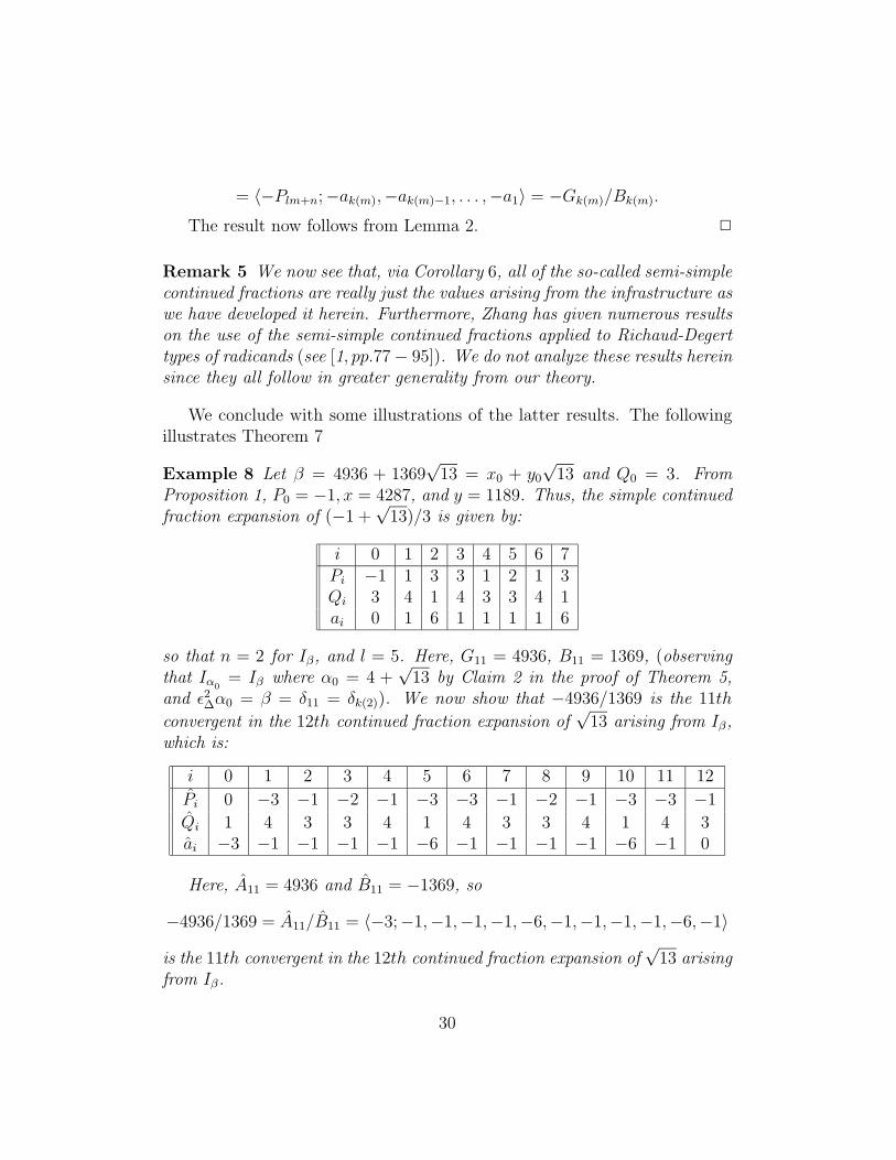
We conclude with some illustrations of the latter results. The followingillustrates Theorem 7

Example 8 Let β = 4936 + 1369√

13 = x0 + y0

√13 and Q0 = 3. From

Proposition 1, P0 = −1, x = 4287, and y = 1189. Thus, the simple continuedfraction expansion of (−1 +

√13)/3 is given by:

i 0 1 2 3 4 5 6 7Pi −1 1 3 3 1 2 1 3Qi 3 4 1 4 3 3 4 1ai 0 1 6 1 1 1 1 6

so that n = 2 for Iβ, and l = 5. Here, G11 = 4936, B11 = 1369, (observingthat Iα0

= Iβ where α0 = 4 +√

13 by Claim 2 in the proof of Theorem 5,and ε2∆α0 = β = δ11 = δk(2)). We now show that −4936/1369 is the 11th

convergent in the 12th continued fraction expansion of√

13 arising from Iβ,which is:

i 0 1 2 3 4 5 6 7 8 9 10 11 12

Pi 0 −3 −1 −2 −1 −3 −3 −1 −2 −1 −3 −3 −1

Qi 1 4 3 3 4 1 4 3 3 4 1 4 3ai −3 −1 −1 −1 −1 −6 −1 −1 −1 −1 −6 −1 0

Here, A11 = 4936 and B11 = −1369, so

−4936/1369 = A11/B11 = 〈−3;−1,−1,−1,−1,−6,−1,−1,−1,−1,−6,−1〉

is the 11th convergent in the 12th continued fraction expansion of√

13 arisingfrom Iβ.

30

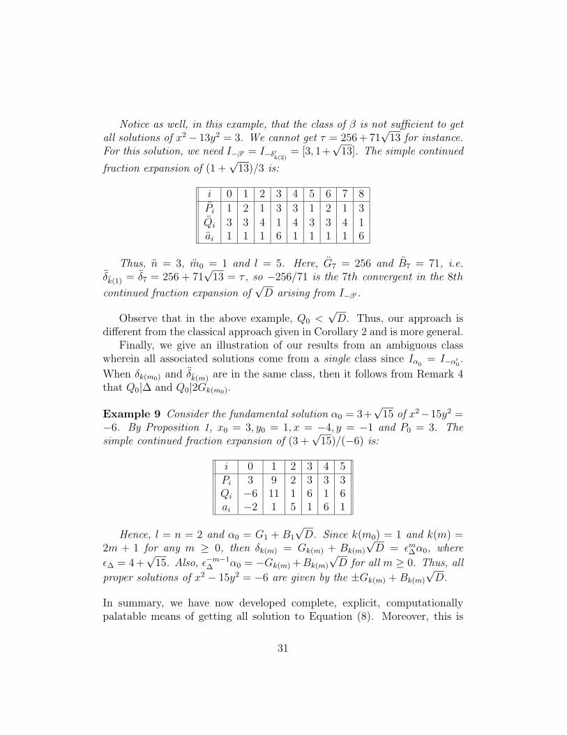
Notice as well, in this example, that the class of β is not sufficient to getall solutions of x2 − 13y2 = 3. We cannot get τ = 256 + 71

√13 for instance.

For this solution, we need I−β′ = I−δ′k(2)

= [3, 1+√

13]. The simple continued

fraction expansion of (1 +√

13)/3 is:

i 0 1 2 3 4 5 6 7 8

Pi 1 2 1 3 3 1 2 1 3

Qi 3 3 4 1 4 3 3 4 1ai 1 1 1 6 1 1 1 1 6

Thus, n = 3, m0 = 1 and l = 5. Here, G7 = 256 and B7 = 71, i.e.δk(1) = δ7 = 256 + 71

√13 = τ , so −256/71 is the 7th convergent in the 8th

continued fraction expansion of√D arising from I−β′.

Observe that in the above example, Q0 <√D. Thus, our approach is

different from the classical approach given in Corollary 2 and is more general.Finally, we give an illustration of our results from an ambiguous class

wherein all associated solutions come from a single class since Iα0= I−α′

0.

When δk(m0) and δk(m) are in the same class, then it follows from Remark 4that Q0|∆ and Q0|2Gk(m0).

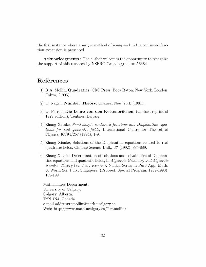
Example 9 Consider the fundamental solution α0 = 3+√

15 of x2−15y2 =−6. By Proposition 1, x0 = 3, y0 = 1, x = −4, y = −1 and P0 = 3. Thesimple continued fraction expansion of (3 +

√15)/(−6) is:

i 0 1 2 3 4 5Pi 3 9 2 3 3 3Qi −6 11 1 6 1 6ai −2 1 5 1 6 1

Hence, l = n = 2 and α0 = G1 + B1

√D. Since k(m0) = 1 and k(m) =

2m + 1 for any m ≥ 0, then δk(m) = Gk(m) + Bk(m)

√D = εm

∆α0, where

ε∆ = 4+√

15. Also, ε−m−1∆ α0 = −Gk(m) +Bk(m)

√D for all m ≥ 0. Thus, all

proper solutions of x2 − 15y2 = −6 are given by the ±Gk(m) + Bk(m)

√D.

In summary, we have now developed complete, explicit, computationallypalatable means of getting all solution to Equation (8). Moreover, this is

31

the first instance where a unique method of going back in the continued frac-tion expansion is presented.

Acknowledgments : The author welcomes the opportunity to recognizethe support of this research by NSERC Canada grant # A8484.

References

[1] R.A. Mollin, Quadratics, CRC Press, Boca Raton, New York, London,Tokyo, (1995).

[2] T. Nagell, Number Theory, Chelsea, New York (1981).

[3] O. Perron, Die Lehre von den Kettenbruchen, (Chelsea reprint of1929 edition), Teubner, Leipzig.

[4] Zhang Xianke, Semi-simple continued fractions and Diophantine equa-tions for real quadratic fields, International Centre for TheoreticalPhysics, IC/94/257 (1994), 1-9.

[5] Zhang Xianke, Solutions of the Diophantine equations related to realquadratic fields, Chinese Science Bull., 37 (1992), 885-889.

[6] Zhang Xianke, Determination of solutions and solvabilities of Diophan-tine equations and quadratic fields, in Algebraic Geometry and AlgebraicNumber Theory (ed. Feng Ke-Qin), Nankai Series in Pure App. Math.3, World Sci. Pub., Singapore, (Proceed. Special Program, 1989-1990),189-199.

Mathematics Department,University of Calgary,Calgary, Alberta,T2N 1N4, Canadae-mail address:ramollin@math.ucalgary.caWeb: http://www.math.ucalgary.ca/˜ ramollin/

32