Embed Size (px)
Citation preview

Eur. Phys. J. C (2020) 80:417https://doi.org/10.1140/epjc/s10052-020-7657-8
Regular Article - Theoretical Physics
All two-loop scalar self-energies and tadpoles in generalrenormalisable field theories
Mark D. Goodsell1,a, Sebastian Paßehr1,2,b
1 Laboratoire de Physique Théorique et Hautes Energies (LPTHE), UMR 7589, Sorbonne Université et CNRS, 4 Place Jussieu, 75252 Paris CEDEX05, France
2 Institute for Theoretical Particle Physics and Cosmology, RWTH Aachen University, Sommerfeldstraße 16, 52074 Aachen, Germany
Received: 26 November 2019 / Accepted: 15 January 2020 / Published online: 13 May 2020© The Author(s) 2020
Abstract We calculate the complete tadpoles and self-energies at the two-loop order for scalars in general renor-malisable theories, a crucial component for calculatingtwo-loop electroweak corrections to Higgs-boson massesor for any scalar beyond the Standard Model. We renor-malise the amplitudes using mass-independent renormali-sation schemes, based on both dimensional regularisationand dimensional reduction. The results are presented herein Feynman gauge, with expressions for all 121 self-energyand 25 tadpole diagrams given in terms of scalar and tensorintegrals with the complete set of rules to reduce them to aminimal basis of scalar integrals for any physical kinematicconfiguration. In addition, we simplify the results to a set ofonly 16 tadpole and 58 self-energy topologies using relationsin order to substitute the ghost and Goldstone-boson cou-plings that we derive. To facilitate their application, we alsoprovide our results in electronic form as a new code TLDR.We test our results by applying them to the Standard Modeland compare with analytic expressions in the literature.
Contents
1 Introduction . . . . . . . . . . . . . . . . . . . . . 21.1 Treatment of tadpoles and application of our
results . . . . . . . . . . . . . . . . . . . . . . 31.2 Guide to the paper . . . . . . . . . . . . . . . . 5
2 Notation and methods . . . . . . . . . . . . . . . . 52.1 Coupling definitions . . . . . . . . . . . . . . . 5
2.1.1 Scalar, vector and fermion couplings . . . 62.1.2 Ghost couplings and ghost flow . . . . . 6
2.2 Processing of diagrams . . . . . . . . . . . . . 72.3 Charged scalars, Dirac fermions and γ5 . . . . 10
3 Removing Goldstone and ghost couplings . . . . . . 11
a e-mail: [email protected] e-mail: [email protected] (corresponding author)
3.1 Ghosts and gauge fixing . . . . . . . . . . . . . 113.2 Goldstone bosons . . . . . . . . . . . . . . . . 123.3 Eliminating all Goldstone-boson couplings . . . 13
3.3.1 Scalar–vector couplings . . . . . . . . . 133.3.2 Scalar–Goldstone couplings . . . . . . . 133.3.3 Fermion couplings . . . . . . . . . . . . 14
4 Results . . . . . . . . . . . . . . . . . . . . . . . . 144.1 Tadpole diagrams . . . . . . . . . . . . . . . . 14
4.1.1 Unreduced diagrams . . . . . . . . . . . 144.1.2 Combined diagrams . . . . . . . . . . . 15
4.2 Self-energies . . . . . . . . . . . . . . . . . . 164.2.1 Unreduced diagrams . . . . . . . . . . . 164.2.2 Combination of classes . . . . . . . . . . 184.2.3 Ghostbusting . . . . . . . . . . . . . . . 184.2.4 Final simplified results for self-energies . 194.2.5 Reduced diagrams of O(g2) . . . . . . . 194.2.6 Reduced diagrams of O(g4) . . . . . . . 194.2.7 Reduced diagrams of O(g6) . . . . . . . 204.2.8 Reducible diagrams containing scalars
and vectors of O(g8) . . . . . . . . . . . 224.2.9 Special topologies: �§,g4
. . . . . . . . . 224.3 Comparison with Landau gauge . . . . . . . . 234.4 Standard Model calculation . . . . . . . . . . . 25
5 Conclusions . . . . . . . . . . . . . . . . . . . . . 25Appendix . . . . . . . . . . . . . . . . . . . . . . . . 26A Integral relations . . . . . . . . . . . . . . . . . . . 26
A.1 Notation and symmetries . . . . . . . . . . . . 26A.2 Reduction of tensor integrals . . . . . . . . . . 27A.3 Reduction of scalar integrals . . . . . . . . . . 27
A.3.1 General relations . . . . . . . . . . . . . 27A.3.2 Reduction rules . . . . . . . . . . . . . . 28
A.4 Vanishing external momentum . . . . . . . . . 31A.5 UV divergences . . . . . . . . . . . . . . . . . 32
B List of renormalised Feynman diagrams . . . . . . . 33B.1 Tadpole diagrams . . . . . . . . . . . . . . . . 33
B.1.1 Known results . . . . . . . . . . . . . . . 33
123
417 Page 2 of 64 Eur. Phys. J. C (2020) 80 :417
B.1.2 New results with vectors . . . . . . . . . 34B.1.3 New results with fermions and vectors . . 36B.1.4 New results with ghosts . . . . . . . . . 36
B.2 Self-energy diagrams . . . . . . . . . . . . . . 37B.2.1 Known results with only scalars . . . . . 37B.2.2 Known results with scalars and fermions . 39B.2.3 Known results with scalars and one vector 40B.2.4 Known results with fermions and one vector 43B.2.5 Known results with scalars, fermions and
one vector . . . . . . . . . . . . . . . . . 44B.2.6 New results with vectors . . . . . . . . . 45B.2.7 New results with fermions and vectors . . 56B.2.8 New results with ghosts . . . . . . . . . 57
References . . . . . . . . . . . . . . . . . . . . . . . . 61
1 Introduction
The Higgs boson mass has been measured to an accuracyof about O(100)MeV, making it an electroweak precisionparameter. In the Standard Model (SM), this is used to extractthe Higgs quartic coupling λ, which, through a significantamount of work can now be done with high precision, whereall of the relevant running parameters of the Lagrangian cannow be extracted from calculations at full two-loop order[1,2] and partially at the three- and four-loop order [3–16]. Acode for calculating λ in Landau gauge, SMH [17], and codesfor extracting all relevant SM parameters (the gauge cou-plings, top and bottom Yukawa couplings, and Higgs quarticcoupling), mr [18,19] (which builds on the results of, interalia, [20–24]) and SMDR [25], exist. As a result of this effort,the uncertainty on the measurement of the top mass is nowmore important than the scalar self-energies in the SM.
However, in theories beyond the Standard Model (BSM),it is not possible to make full use of the Higgs-mass mea-surement because the theoretical uncertainty on the masscalculation can be much larger, owing to the new degrees offreedom. As a result, an enormous amount of effort has goneinto refining the calculation of the Higgs-boson mass froma given set of physical or top-down inputs, in both genericand specific theories. This has typically been driven by theneed for accurate predictions of the Higgs mass in supersym-metric models, where the Higgs quartic coupling is predictedfrom the gauge couplings (and other top–down parametersin extended models).
The early expectation was for new coloured supersymmet-ric particles near the electroweak scale, and since the Min-imal Supersymmetric SM (MSSM) had a tree-level upperbound on the Higgs mass equal to the mass of the Z boson,a full fixed-order calculation in the MSSM at the one-looporder [26–35] is vital, but the results at the two-loop order areknown to contribute several GeV to the SM-like Higgs-bosonmass. After much work a full fixed-order two-loop result is
still not available: public codes use an effective-potential cal-culation (neglecting the external momentum) in the “gauge-less limit” (neglecting the electroweak gauge couplings) withresults in the “real MSSM” (neglecting CP phases) [36–53]and in the “complex MSSM” (including CP violation) [54–64]. Some results also exist for three-loop strong correctionsin the effective-potential limit, see Refs. [65–68], now avail-able in the Himalaya package [69,70] which also includesfour-loop leading logarithms of the strong corrections.
Some results now also exist beyond the gaugeless/effective-potential limit: a complete effective-potential cal-culation was described in Refs. [47,50], where the effectivepotential was computed and the derivatives taken numeri-cally, but application of this was hampered by theGoldstone-Boson Catastrophe (GBC) which we shall discuss below.Contributions of O(
(αt + αb + ατ )2) [71], O(αt αs) [72–
74], O(α αs) [73], and O((αt + αb + α) αs) [75] with non-vanishing external momentum were computed in fixed-ordercomputations.1 However, there is now some urgency to fill inthe remaining discrepancy of the full electroweak correctionsand include momentum dependence (which are of the samenominal order for the SM-like Higgs boson) – these haveremained a “holy grail” of the community for some time.
If new particles beyond the SM are very heavy com-pared to the electroweak scale, a fixed-order calculationbreaks down due to large logarithms, and an effective-field-theory (EFT) approach (or a hybrid approach, see Refs. [76–84]) should be used. Such techniques have been applied forsome time [85–96], but it has been found that the thresholdcorrections when matching on to the SM (or split supersym-metry, or Two-Higgs-Doublet Model) can be large. Indeed,while the two-loop renormalisation group equations (RGEs)have been known since the 90s, the one-loop threshold cor-rections in the MSSM were only evaluated recently [97–99],and followed by an extraction of the same two-loop correc-tions that are available for fixed-order computations [99–102], essentially by matching the masses of the lightest Higgsboson in the MSSM and the SM at the EFT matching scale.Indeed, as discussed in Refs. [77,103], a fixed-order calcu-lation can always be used to extract threshold correctionsin this way, especially when the low-energy theory containsonly one scalar field such as in the SM. Hence developmentof fixed-order and EFT calculations go hand in hand.
Since the MSSM has been the driver for much of this work,the accompanying work on other theories has been much lessdeveloped until recently: in the next-to-MSSM (NMSSM),fixed-order calculations were done at the one-loop order[104–115] with only the dominant two-loop corrections in the
1 We make use of the common notation that αi ≡ g2i /(4 π) where gi
is a given coupling; α ≈ 1/137 corresponds to the electric coupling,while gs , gt , gb correspond to the strong gauge, top Yukawa and bottomYukawa couplings.
123

Eur. Phys. J. C (2020) 80 :417 Page 3 of 64 417
effective-potential approach of O((αt + αb) αs) [107,116]and O(
α2t
)[117] explicitly available; for Dirac-gaugino
models, the O(αt αs) corrections were computed in Ref.[118].
However, particularly given the absence of clear signs ofnew physics from the Large Hadron Collider (LHC), it is sen-sible to take a model-agnostic approach where possible, andthis has led to a program ofgeneric calculations. In Ref. [119]the full effective potential was given for general renormalis-able theories in Landau gauge. This was then implementedin the package SARAH in Ref. [120] in the gaugeless limit,where the first and second derivatives of the potential weretaken numerically. This allowed, for the first time, two-loopcorrections to be computed for anymodel at the push of a but-ton. Moreover, in Ref. [121], scalar self-energies for generaltheories were computed up to second order in the gauge cou-plings. This is sufficient for a gaugeless-limit computation ofthe Higgs mass, however the tadpole diagrams were lacking.In Ref. [122] these were computed, and the self-energiessimplified to the effective potential limit – the result beingagain implemented in the package SARAH. However, even inthe gaugeless effective-potential limit, this calculation wasplagued by the GBC. The solution came for the general casein Ref. [123], and was implemented in SARAH with someadditional developments to the method in Ref. [124]. Thisnow represents the state-of-the art for any theory – supersym-metric or otherwise – other than the SM or MSSM (for exam-ple, Refs. [125,126] describe the only calculations includingall superpotential terms in the NMSSM), and in fact pro-vides the only calculation including flavour-violating effectsat the two-loop order [127], or with pure DR
′renormalisa-
tion for the complex MSSM [126]. The status for thresholdcorrections lags somewhat behind: generic thresholds at theone-loop order were computed in Refs. [103,128], where inparticular the former reference describes the consistent treat-ment of infra-red divergences and counterterm choices thatcan simplify the computation, while the latter described theimplementation in SARAH.
The purpose of this work is to finally complete the set ofscalar self-energy diagrams in the gauge coupling for generalrenormalisable theories, and provide the tadpole diagrams atthe same time. This completes the set that was promised inRef. [121]. In this paper we present the analytic expressionsand the technical machinery that we have used, specialisingto the Feynman gauge. However, since the final results (andtherefore this paper) are rather long, we have created a newpackageTLDRwhere they are available in computer-readableform. Readers wishing to skip the details and apply the resultsare invited to download the code from:
http://tldr.hepforge.org
While some of the evaluation of spinor/Lorentz traces andtensor reduction for specific models could be accomplished
using TwoCalc [129] and TARCER [130] (of which wehave made use) we derived some reduction rules not avail-able there with the help of the general relations of Refs.[131,132], so that all results can be reduced to a basis ofjust a few one- and two-loop scalar functions that can benumerically evaluated in TSIL [133]. Moreover, our resultsare already renormalised, and in particular we reduce thenumber of classes of diagrams by making extensive use ofidentities relating couplings of ghosts and Goldstone bosonsto other couplings in the theory.
Our calculation can be used for:
• Corrections to charged and/or coloured scalar masses.For example, in supersymmetric theories this wouldmean e.g. squark or sgluon masses.
• Electroweak corrections to the Higgs-boson mass ↔extraction of Higgs/neutral scalar quartic couplings.These ought to be supplemented by a two-loop extrac-tion of the electroweak expectation value and gauge cou-plings (which requires the two-loop corrections to muondecay and vector-boson self-energies, which we hope toreturn to in future work).
• EFT matching of the Higgs quartic coupling via the pole-mass matching technique [77]. As described at one-looporder in Ref. [103], although a priori this would seem torequire a calculation of the Z -boson mass, in fact all ofthe necessary information is contained in the scalar self-energies/tadpoles, and thus the calculations here may besufficient.
1.1 Treatment of tadpoles and application of our results
The main application of our results is expected to be the eval-uation of the pole mass for scalar bosons in any given theory.For a general theory with scalars having indices i, j, . . . andmasses m2
i at the tree level, this corresponds to finding the(complex) solutions of the equations
0 = Det[(
p2 − m2i
)δi j − �i j
(p2
)], (1)
in p2, where �i j (p2) is the self-energy. We then write
�i j (p2) = �
(1)i j + �
(2)i j + · · · (2)
where the superscripts denote the order of perturbation the-ory.
There are three main techniques used to solve this in prac-tice. The first is to iteratively evaluate Eq. (1) by startingwith p2 = m2
i ; this does not respect gauge invariance orperturbation order. The second is to perturbatively expandthe momentum as p2 = m2
i + p21 + p2
2 + · · · and use matrixperturbation theory to extract the pole mass at each order;
123

417 Page 4 of 64 Eur. Phys. J. C (2020) 80 :417
this gives a gauge invariant result which respects the orderof perturbation theory, but can be tricky to implement in thecases of some masses being degenerate. The third method(see Ref. [121]) is to solve
0 = Det[(
p21 − m2
i
)δi j − �
(1)i j
(m2i
)](3)
iteratively, then expand the one-loop self-energy, giving
�(2)i j
(p2
)→�
(1)i j
(m2i
)+
(p2
1 − m2i
)�
(1) ′i j
(m2i
)+�
(2)i j
(m2i
),
(4)
and insert into Eq. (1) to solve for p22, and so on. This method
is gauge invariant but does not respect the perturbation orderin p2, since p2
1 will contain contributions from[�
(1)i j
(m2i
)]2
and higher powers, etc. In particular, if the aim is to use thepole-mass-matching procedure to extract threshold correc-tions, then the first or third methods will lead to uncancelledhigher-order logarithms.
We therefore recommend the use of the second approach,whereby the pole mass at the two-loop order is simply
p2pole,i = m2
i + �(1)i i
(m2i
)+ �
(2)i i
(m2i
)
+ �(1)i i
(m2i
)�
(1) ′i i
(m2i
)
+∑
j
1
m2i − m2
j
�(1)i j
(m2i
)�
(1)j i
(m2i
), (5)
and where the one-loop self-energies have already been diag-onalised on the subspace of states that are degenerate at thetree level; the sum over j includes all scalar and vector stateswith the same quantum numbers.
In general, it is also necessary to include the contribu-tions of tadpole diagrams. This is because, for each neu-tral scalar with a non-trivial expectation value, there is anon-trivial vacuum minimisation condition, which can beused to eliminate one parameter from the theory. Commonly,parameters of mass dimension 2 are substituted in this step,such as the μ2 |H |2 term in the Higgs potential of the SM.If we write the neutral component of the Higgs field asH0 = 1√
2(v + h + · · · ) and the quartic term as λ |H |4, then
the necessary condition for the vacuum being a minimum is
0 = μ2 v + λ v3 + ∂V
∂h(6)
where V are the loop corrections to the effective potential;its derivatives correspond to tadpole diagrams. If we insistthat v is the correct vacuum expectation value to all looporders, then we can eliminateμ2 wherever it appears in favourof λ v2 and tadpoles. Formally, then we can expand
μ2 = −λ v2 − 1
v
∂V (1)
∂h− 1
v
∂V (2)
∂h− · · · (7)
where the superscripts denote loop orders. Since the tree-level Higgs mass is m2
h = μ2 + 3 λ v2, this means that thetadpole contributions modify the Higgs mass at higher orders.
Utilising this method for the computation of the mass ofany particle in the theory that depends on μ2 requires thecalculation of self-energies and tadpole diagrams. In partic-ular, the application to computing the mass of the Goldstonebosons leads to the GBC: in Landau gauge the “tree level”Goldstone mass squared becomes of one-loop order and isof indeterminate sign, which causes infra-red singularities inthe two-loop tadpoles and self-energies [134,135]. The ini-tially proposed solution was to resum Goldstone diagrams,and this was performed for the tadpoles of the MSSM in Ref.[136]. However, in general this is cumbersome to implement;and general solutions now exist for both, tadpoles and self-energies, where we can instead use an “on-shell” mass forthe Goldstone bosons [123], or just perturbatively expand thegeneralisations of Eq. (7) to the loop order that we are work-ing to in tadpoles and self-energies [124], known as taking“consistent tadpole equations”; for example, we would needto take
�(2)i j
(p2
)→ �
(2)i j
(p2
)∣∣∣μ2=−λ v2
− 1
v
[∂�
(1)i j
(p2
)
∂μ2
∂V (1)
∂h
]
μ2=−λ v2
. (8)
In this way, the infra-red singularities cancel between the twoparts on the right-hand side, and this should continue orderby order in perturbation theory.
Another way of treating tadpoles is to work only in termsof running parameters, so our expectation values solve thetree-level vacuum-minimisation conditions only. That meansthat we must include tadpole diagrams as part of the selfenergies: these are one-particle irreducible but contain prop-agators carrying no momentum (referred to as “internal”).This was the approach used in the SM calculation of Ref.[18] and leads to a gauge-invariant result, without needing toperform expansions of the form of Eq. (7), at the expense ofa proliferation of diagrams, such as those depicted in Fig. 1.
In this paper, we shall work in the Feynman gauge. Primafacie, one would think that our results do not suffer frominfra-red singularities, and so we sidestep the GBC, and couldavoid making an expansion of the form of Eq. (7): we could(as originally envisaged in Ref. [121]) just modify μ2 at thetree level so that Eq. (6) is satisfied and dispense with anyextra diagrams or shifts of the form of Eq. (8). A reader wish-ing to implement this program can use the results from theAppendix (121 self-energy classes and 25 tadpoles) or thereduced set of 89 self-energy diagrams described in Sect. 4.
123

Eur. Phys. J. C (2020) 80 :417 Page 5 of 64 417
Fig. 1 Examples of one-particle-irreducible diagrams with “internal”propagators that we do not include in our list of topologies. All diagramsof these classes can be straightforwardly computed from the one- andtwo-loop self-energies and tadpoles that we include here
However, such an approach does not respect the order ofperturbation theory or gauge invariance.2 Hence, we shallsimplify the expressions where all couplings and masses areexpressed in terms of tree-level parameters, so that the readermay use any of the other approaches. In this way, we arealso able to make extensive use of relationships amongst thecouplings in general theories, and so reduce the number oftopologies to 16 for tadpoles and to 58 for self-energies fornon-Goldstone boson scalars.
To apply the results in practice for all but the simplestof models is a task for a computer. Even for the StandardModel it would be far too tedious to implement by hand.Hence, we have provided our results in electronic form aspart of TLDR. All reduction rules are included so that therenormalised expressions can be applied for any physicallyrelevant configurations of masses and momenta, in the formof Mathematicamodules and notebooks, with code to linkfrom Mathematica to TSIL. A user manual is providedonline. In the future we also intend to include c++ codeto link to TSIL for use with packages such as SARAH, the(currently private) results for Landau and general Rξ gauges,and extensions to vector/mixed scalar–vector/fermion self-energies.
1.2 Guide to the paper
The paper is organised in the following way:
• in Sect. 2 we introduce our nomenclature for the fields andcouplings that appear in renormalisable theories, and weexplain our method of computing the two-loop diagramsand counterterms. As our results are valid for real fields,we also show how to apply them to complex scalars andDirac fermions.
2 Moreover, theories with genuine Goldstone bosons would still suf-fer the GBC. Hence, in our integral reductions, we must still deal withFootnote 2 continuedinfra-red singularities. In this work, we do so by means of dimensionalregularisation: all infra-red divergent diagrams acquire poles in thedimensional regulator ε. This actually provides yet another solution tothe GBC; we shall elaborate on the connection more clearly elsewhere.
• The purpose of Sect. 3 is to reduce the number of differentdiagrams by making use of relations among the couplingsthat are dictated by gauge invariance. In this way, ghostsand Goldstone bosons can be eliminated from the theory.
• The nomenclature that is used for the loop integrals isintroduced in Appendix A. There, we also describe howeach integral can be reduced for any kinematic configu-ration into a basis that can be quickly evaluated numeri-cally.
• The full list of results for renormalised two-loop tadpolesand self-energies in terms of the previously defined cou-plings and loop integrals is given in Appendix B.
• The substitution of ghost and Goldstone couplings isapplied to these results in Sect. 4. In the same section,we also compare to previously known expressions.
• Our conclusions are summarised in Sect. 5.
2 Notation and methods
In this section we shall give our definitions and methods,needed to understand the results presented in Sect. 4 and theAppendix.
2.1 Coupling definitions
In Ref. [121], scalar self-energies were given using two-component spinors and a compact notation in terms of cou-plings in a general lagrangian. Such a lagrangian reads
L = LS + LSF + LSV + LFV + Lgauge + LSghost, (9)
where
LS ≡ −1
6ai jk i j k − 1
24λi jkl i j k l ,
(10a)
LSF ≡ −1
2y I Jk ψI ψJ k − 1
2yI Jk ψ
Iψ
J k , (10b)
LFV ≡ gaJI Aaμ ψ
Iσμ ψJ , (10c)
LSV ≡ 1
2gabi Aa
μ Aμb i + 1
4gabi j Aa
μ Aμb i j
+ gai j Aaμ i ∂
μ j , (10d)
Lgauge ≡ gabc Aaμ Ab
ν ∂μAνc − 1
4gabe gcde Aμa Aνb Ac
μ Adν
+ gabc Aaμ ωb ∂μωc , (10e)
LSghost ≡ ξ gabi i ωa ωb. (10f)
The fields i with indices {i, j, k, l} denote real scalars, ψI
with indices {I, J, K , L} Weyl fermions, Aaμ with indices
{a, b, c, d} gauge bosons, and ωa, ωa ghosts and antighosts
123

417 Page 6 of 64 Eur. Phys. J. C (2020) 80 :417
(which carry gauge-boson indices). The Eq. (10) slightly dif-fer from the ones in Ref. [121] because we work with adifferent metric signature (+,−,−,−) and, since we workaway from the gaugeless limit/Landau gauge, we have cou-plings between scalars and ghosts.
2.1.1 Scalar, vector and fermion couplings
In this work, due to the large numbers of diagrams and thecomplexity of the expressions, we perform the generic cal-culations using computer algebra, and we expect that theapplication of the results will be best accomplished by imple-mentation on computers. Hence, we use coupling definitionsthat are more practical for that case; indeed, since we useFeynArts to generate the set of generic diagrams, we adoptan abbreviated form of the notation of the generic model fileLorentz.gen. FeynArts works in four-spinor notationand distinguishes particles and antiparticles; we remove thisdistinction in our results by transforming all fields to realscalars, gauge bosons and Majorana fermions. Our resultsare therefore given in terms of vertices which, in general,have more than one possible Lorentz structure; we denotethis with an index as last argument of each coupling. Ourvertices are named by their adjacent particles, S for scalars,F for fermions,V for vectors, andU for ghosts. The dictionarywith Eq. (10) is:
SSS[i, j, k, 1] = ai jk, (11a)
SSSS[i, j, k, l, 1] = λi jkl , (11b)
FFS[I, J, i, 1] = y I J i ,
FFS[I, J, i, 2] = yI J i =(y I J i
)∗, (11c)
FFV[I, J, a, 1] = −gaJI ,
FFV[I, J, a, 2] = −FFV[J, I, a, 1] = (FFV[I, J, a, 1])∗ ,
(11d)
SVV[i, a, b, 1] = −gabi , (11e)
SSVV[i, j, a, b, 1] = −gabi j . (11f)
For the terms with fermions, the Lorentz structure withindex 1 or 2 refers to a left- or right-chiral projector, respec-tively; the FFV couplings contain a gamma matrix in addi-tion.
The remaining couplings require more inspection. TheSSV vertex is given by
ı ∂3
∂ i ∂ j ∂Aμa
[ga
′i ′ j ′ Aμa′ i ′
(ı pμ
j ′)
j ′]
= −gai j pμaj − gaji pμa
i = gai j(pi − p j
)μa
= SSV[i, j, a, 1] pμai + SSV[i, j, a, 2] pμa
j , (12a)
→ SSV[i, j, a, 1] = ı gai j ,
SSV[i, j, a, 2] = −SSV[i, j, a, 1]. (12b)
We note that we do not enforce the equality of the two termsfor the counterterm vertex.
Next, for the pure gauge-coupling terms, we have (ημν isthe Minkowski metric)
ı ∂3
∂Aμa ∂Aμb ∂Aμc
[gabc Aa′
μ Ab′ν
(ı pμ
c
)Aνc′]
= −gabc[ημaμb
(pμcb − pμc
a
) + ημbμc(pμac − pμa
b
)
+ ημcμa(pμba − pμb
c
)], (13a)
→ VVV[a, b, c, 1] = −ı gabc. (13b)
For the four-vector coupling, we have the generic vertex
ı ∂4
∂Aμa ∂Aμb ∂Aμc ∂AμdL
= −2 ı[gabe gcde ημaμb ημcμd + gace gbde ημaμc
ημbμd + gade gcbe ημaμd ημcμd]
= −ı[VVVV[a, b, c, d, 1] ημaμb ημcμd
+ VVVV[a, b, c, d, 2] ημaμc ημbμd
+VVVV[a, b, c, d, 3] ημaμd ημcμb], (14a)
and thus we have the identifications
VVVV[a, b, c, d, 1] = −2VVV[a, c, e, 1]VVV[b, d, e, 1], (14b)
VVVV[a, b, c, d, 2] = −2VVV[a, b, e, 1]VVV[c, d, e, 1], (14c)
VVVV[a, b, c, d, 3] = 2VVV[a, d, e, 1]VVV[b, c, e, 1] (14d)
with a sum on e.
2.1.2 Ghost couplings and ghost flow
Finally, for the ghost terms, in theFeynArtsgeneric model,no particular form of the couplings is enforced: the generalvertex for the UUV coupling is equal to
−ı UUV[a, b, c, 1] pμca − ı UUV[a, b, c, 2] pμc
b , (15)
whereas from Eq. (10) we see that in general Rξ gauge oneof these terms is always vanishing because the vertex onlycontains a ghost and antighost (not ghost–ghost or antighost–antighost) and moreover only contains a factor of the momen-tum of the antighost. Hence we must preserve the distinctionbetween ghost and antighost in our amplitude, and we shouldalso include both directions of ghost flows. Then we have
UUV[−a, b, c, 1] = VVV[a, b, c, 1], UUV[−a, b, c, 2] = 0,
(16a)
UUV[a,−b, c, 1] = 0, UUV[a,−b, c, 2] = −VVV[a, b, c, 1],(16b)
123

Eur. Phys. J. C (2020) 80 :417 Page 7 of 64 417
Top. 1 Top. 2 Top. 3
Top. 1 Top. 2 Top. 3 Top. 4 Top. 5 Top. 6 Top. 7 Top. 8 Top. 9
Fig. 2 All possible topologies of one-particle irreducible Feynman dia-grams for two-loop tadpoles (top row) and self-energies (bottom row)are shown.In Ref. [121] the self-energy topologies are referred to as Y ,
U ,U , M , V , X , Z , W , S respectively (topologies 2 and 3 are equivalentfor identical incoming/outgoing states)
SUU[i, a,−b, 1] = −ξ gbai , SUU[i,−a, b, 1] = −ξ gabi .(16c)
The signs here are confusing, because we expect that theghosts are anticommuting, and so should be the vertices. Thisis an artefact of the algorithm used to construct the ampli-tudes, where the ordering of the indices in the couplings isnot meant to be taken literally: it is assumed that for a givenchoice of particles in a vertex, either there is only one wayof combining them into a vertex, and this is the ordering thatis implied (e.g. for a scalar–ghost–antighost coupling thereis only one correct choice), or the ordering does not matter.
However, there are two good reasons that the reader doesnot need to worry about this issue: the first is that they can justtake the above prescriptions and plug them into our results,given in the ESM Appendix. Importantly, for the ghost ampli-tudes they should sum over both signs of each ghost index,e.g. for diagram I(2)
025 we have the result
SSS[i1, i3, i6, 1]SUU[i2,−i7, i4, 1]SUU[i3,−i4, i5, 1]SUU[i6,−i5, i7, 1] × loopfunction (17a)
that should be interpreted as
(ai1,i3,i6 gi2,i4,i7 gi3,i5,i4 gi6,i7,i5
+ai1,i3,i6 gi2,i7,i4 gi3,i4,i5 gi6,i5,i7)×loop function. (17b)
However, the second reason to not worry about this is that inSect. 3 we demonstrate how all of the ghost couplings can beremoved from the amplitude, giving a much smaller numberof classes of diagrams to evaluate.
2.2 Processing of diagrams
Here we describe our approach to generating and renormal-ising the diagrams.
Feynman-diagrammatic approach: The two-loop Feyn-man diagrams are generated with the help of FeynArts
[137–139]. The different one-particle irreducible topologiesof tadpoles and self-energies are depicted in Fig. 2. Each ofthese topologies is populated with all possible combinationsof fermions F (straight lines), scalars S (dashed lines), vec-tor bosons V (wavy lines), and ghosts U (dotted lines) inrenormalisable theories. The external legs are fixed to bescalars. Each particle in the diagram is assigned a uniqueindex ∈ {i1, . . . , i7} for full generality.
BPHZmethod: In general, the integrals of the two-loop dia-grams in Fig. 2 are ultra-violet (UV) divergent. In order to reg-ularise them, we follow the BPHZ prescription [140–143].Each two-loop diagram contains UV-divergent sub-loops ofone-loop order that can be regularised by appropriate coun-terterms. In general, an additional two-loop counterterm isnecessary in order to regularise all UV poles. While the lattercan be defined as a pure polynomial in the UV regulator 1/ε,the former regularise all non-local divergences and in generalgive rise to UV-finite terms as well.
The realisation of the splitting of two-loop diagrams intothe so-called forest of sub-loop diagrams is carried out inan automated way. For each sub-loop diagram, the corre-sponding one-loop diagram with counterterm insertion isgenerated. In addition, the appropriate counterterm topologythat regularises the logarithmic divergence of this sub-loopis determined automatically. The algorithm is based on agraph-theoretical interpretation of Feynman diagrams: first,the closed cycles (loops) of each diagram are identified; sec-ond, for each cycle, the lines (internal propagators) that makeup the loop are shrunken into a point (counterterm vertex);third, the adjacencies to the shrunken cycle in the originaldiagram (and the cycle itself) are used in order to determinethe required counterterm insertion. An illustrating exampleof this procedure is given in Fig. 3.
Symmetry factors: Analytical results in terms of ampli-tudes for the genuine, generic two-loop diagrams as wellas the corresponding one-loop diagrams with countertermvertex, and the one-loop counterterm insertions are gener-ated with the help of FeynArts, FormCalc [144,145]
123

417 Page 8 of 64 Eur. Phys. J. C (2020) 80 :417
Fig. 3 The different sub-loops of topology 2 of the self-energies inFig. 2 are marked in red at the left column. After shrinking the linesof these sub-loops, the remaining one-loop diagrams with countertermvertex are displayed at the middle column. The appropriate countert-erm insertion for each counterterm vertex is given at the right column.
The consecutive numbers at the lines label the propagators; the samenumber in the diagrams of one row refers to the same particle at thatpropagator. A signed number indicates the antiparticle to the unsignedone (note that external particles are defined as incoming by default)
and TwoCalc [129] (we also make use of OneCalc that ispart of TwoCalc). Note that among the 121 different self-energy and 25 different tadpole diagrams that FeynArtsgenerates, those diagrams with symmetries of internal prop-agators have already been removed, whereas diagrams withsymmetries with respect to the external propagators are allkept. This processing fixes the symmetry factors of the gen-uine two-loop diagrams. The symmetry factors of the coun-terterm diagrams are modified accordingly in order to matchthe regularised two-loop diagram.
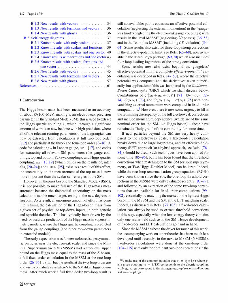
Couplings: All occurring couplings are re-labelled by thesequence of acronyms for all adjacent fields and carry thecorresponding propagator indices as argument. An additionalnumeric argument � at the last position allows one to distin-guish the couplings of the same fields with different Lorentzstructure, as described in Sect. 2.1 where we give the dic-tionary to parameters in the Lagrangian. In FeynArts thepropagator indices may be signed in order to refer to antipar-ticles.3 The different Lorentz structures of the couplingsare summarised in Appendix A of the FeynArts manual[139]; the argument � refers to the �th entry of the vectorof couplings. The only deviation from the default setup ofthe Lorentz structure applies to the coupling SSV[ia, ib, ic]that depends on the momenta kia and kib of the scalar fields:
3 Note that at this stage the fields F,S,V,U are not yet specified andmay themselves be physical antiparticles. Therefore, a signed index ofan antiparticle refers to the particle.
at the level of the counterterm vertices not all instances areproportional to (kia − kib); instead, the dependence on kia
and kib needs to be distinguished. For this purpose, the defaultgeneric model file (and the model file) of FeynArts is ini-tialised with the modifications given in Fig. 4; for the cou-plings (rather than counterterms) we keep the original ver-tex SSV[ia, ib, ic, 1].4
Counterterm vertices: Since the same counterterm vertexcan emerge from shrinking sub-loops of different two-loopdiagrams, it is mandatory to store information about the two-loop topology along with the counterterm vertex in orderto determine the appropriate insertion. Our choice is to stayclose to the existing description in FeynArts, and to assigna canonically ordered list of edges to each Feynman dia-gram. The edges correspond to the propagators (includingthe field type) of the diagram. The propagator indices arestored as well since they are required for correctly labellingthe counterterm insertions; for the purpose of sorting or iden-tifying diagrams they are not considered. Due to the canoni-cal ordering of the edges, the direction of a propagator mightbe reversed. In that case, the propagator index of that linereceives a sign, indicating an antiparticle. An example ofthis correspondence is shown in Fig. 5.
4 The generic model file Lorentz.gen is utilised together with themodel file SM.mod. The latter is required in order to load all structuresfor FeynArts. It already contains all possible renormalisable genericcouplings.
123
Eur. Phys. J. C (2020) 80 :417 Page 9 of 64 417
SetOptions[InitializeModel,GenericModelEdit :> (M$GenericCouplings = M$GenericCouplings /.AnalyticalCoupling[s1 S[j1, mom1], s2 S[j2, mom2], s3 V[j3, mom3, {li3}]] == _ :>AnalyticalCoupling[s1 S[j1, mom1], s2 S[j2, mom2], s3 V[j3, mom3, {li3}]] ==G[-1][s1 S[j1], s2 S[j2], s3 V[j3]].{FourVector[mom1, li3], FourVector[mom2, li3]}
),ModelEdit :> (M$CouplingMatrices = M$CouplingMatrices /.(c : C[s1_. S[j1_], s2_. S[j2_], s3_. V[j3_]]) == {exp_} :> c == {exp, -exp}
)];InitializeModel["SM"];
Fig. 4 The default generic model file of FeynArts is modified in order to allow for different Lorentz structures of the coupling SSV
S(i1) S(i2)
S(i3)
V(i4)
F(i5)
F(i6)
V(i7) {edge[iv[1], v[2], S[i1]], edge[iv[3], v[4], S[i2]],edge[v[2], v[4], S[i3]],edge[v[2], v[5], V[-i4]], edge[v[4], v[6], V[-i7]],edge[v[5], v[6], F[-i5]], edge[v[5], v[6], F[-i6]]}
Fig. 5 Each Feynman diagram can be uniquely identified by the listof its edges when interpreted as a graph. Each edge has three argu-ments: a starting vertex, an ending vertex, and a label (describing fieldtype and propagator index). The vertices v[i] are numbered consecu-tively, i ∈ N. The starting vertices of external fields are not connected to
the other edges and labelled iv[i]. If the starting and ending verticesof an edge are interchanged compared to their original description inFeynArts, the propagator index receives a sign, indicating an antipar-ticle on that line
Counterterm insertions: All one-loop one-point, two-point,three-point and four-point processes were computed at thegeneric level using FormCalc, since they can in princi-ple appear as counterterm insertions. Each of the Feynmandiagrams that appears in these processes was evaluated sep-arately and stored together with its list of edges. In this way,individual results can be looked up quickly and inserted intothe correct counterterm vertex; they may in future be pro-vided as part of TLDR. In fact, to evaluate our results weuse a separate algorithm to calculate just the divergent partsof the counterterms (which are identical in MS or DR at theone-loop order) on the fly, and which works in any gauge.
Gauge fixing and regularisation: All two-loop self-energyand tadpole diagrams, the corresponding one-loop diagramswith counterterm vertex, and the UV divergences of thecounterterm insertions have been determined in ’t Hooft–Feynman gauge, Landau gauge, and the general Rξ gauge.However, diagrams with a large number of gauge bosons caninitially be expressed in a much shorter form in ’t Hooft–Feynman gauge. For this reason, we performed the com-
plete integral reduction only for the Feynman gauge (seeAppendix A). In addition, we computed our results usingdimensional regularisation (for MS renormalisation), anddimensional reduction (for DR renormalisation). The extraterms in dimensional regularisation have a coefficient δMS.
Results: The outcome for the combination of each genuinetwo-loop integral with the corresponding counterterms forall sub-loops is given in Appendix B.1 for the tadpoles,and in Appendix B.2 for the self-energies; first, all previ-ously known expressions of Refs. [121,122] are given in ournomenclature, and then all new results are stated. Note thatthe pure UV divergent two-loop counterterms are not con-tained in these results, as they simply add clutter to the expres-sions. After carrying out the integral reduction and extractingall UV divergences via the relations in Appendix A, polyno-mials in the regulator 1/ε will remain, which simply corre-spond to the genuine two-loop counterterm of the diagram;but we may also find additional divergent and finite partscorresponding to any infra-red divergences: we do not intro-duce infra-red counterterms. As described in Sect. 1.1 any
123

417 Page 10 of 64 Eur. Phys. J. C (2020) 80 :417
infra-red divergences should cancel in a full amplitude whencombined with one-loop self-energy and tadpole diagrams.Basis of loop integrals: We have provided all of the integralreduction rules in Appendix A to extract the finite part ofour generic renormalised amplitudes for any kinematic con-figuration in terms of the basis of one- and two-loop scalarfunctions that can be evaluated in TSIL. This is a basis of sixtwo-loop scalar integrals and two one-loop ones. The TSILbasis are actually “renormalised” integrals, with specific sub-tractions; essentially they can be built up from Ref. [146]:
S(x, y, z) = limε→0
{S(x, y, z) − 1
ε[A(x) + A(y)
+A(z)] − 1
2 ε2 [x + y + z]
− 1
2 ε
[p2
2− x − y − z
]}, (18a)
U (x, y, z, u) = limε→0
{U(x, y, z, u) − 1
εB(x, y)
+ 1
2 ε2 − 1
2 ε
}, (18b)
M(x, y, z, u, v) = limε→0
M(x, y, z, u, v), (18c)
where the definitions of the boldtype integrals are given inAppendix A.3.1, and the number of spacetime dimensionsis d = 4 − 2 ε. In our results in the Appendix we use theequivalent of the boldtype integrals, and so when taking thefinite part of the diagram we must use
Fin[S(x, y, z)] = S(x, y, z) − x B∣∣ε1
0 (0, 0, x)
− y B∣∣ε1
0 (0, 0, y) − z B∣∣ε1
0 (0, 0, z),
(19a)
Fin[U(x, y, z, u)] = U (x, y, z, u) + B∣∣ε1
0
(p2, x, y
), (19b)
where Fin[. . .] denotes the finite part as ε → 0, i.e.neglectingnon-zero powers of ε, and
B∣∣ε1
0
(p2, x, y
)≡ Fin
[1
εB(x, y)
]. (20)
In principle, since B(x, y) is known analytically to all ordersin ε, it is not difficult to evaluate B|ε
0 (and it is even avail-able in TSIL). However, its presence is a sign of an infra-red divergence: in the absence of infra-red divergences, allB|ε
0 integrals cancel in the renormalised amplitude. We haveexplicitly checked that this is the case for all the results inthe Appendix. So then the reader might be curious as to whywe do not give the results in terms of the renormalised TSILbasis, as done in Ref. [121]; the reasons are twofold:
• Diagrams with vector bosons contain many more tensorintegrals. By listing them in unreduced form we are ableto give our results for each diagram in only a few lines,whereas some diagrams could fill pages by themselves inexpanded form, even just for the most general case wherethere are no vanishing or degenerate masses.
• The integral reduction depends crucially on whether thereare coincident or vanishing masses. The simplest casesconcern scalar integrals with repeated propagators, wherefor non-identical masses we can use partial fractions toreduce them (see Eq. (121)). In Ref. [121] there were gen-erally one or two such cases per integral. In the imple-mentation of the results of Refs. [123,124] in SARAH,one scalar integral contains 12 different reductions. How-ever, in our results, we also have cases in the reduc-tion where some vanishing gauge-boson or ghost massesnaively lead to poles; furthermore, there are also specialcases with the external momentum taken equal to thescalar mass that are relevant (in particular) for chargedscalar propagators. Hence our results (for example forI(2)
086) have up to 47 different special kinematic configu-rations! In TLDR we provide the different special casesfor each diagram, and our reduction rules transform themto the appropriate renormalised integral; clearly it wouldbe impractical (and not especially useful) to list all of thefinal results here.
2.3 Charged scalars, Dirac fermions and γ5
Our results are calculated using Majorana four-spinors,and in Sect. 2.1 we gave a prescription of how to trans-late them to Weyl-spinor notation – but under the condi-tion that the spinors are also Majorana, i.e. have diago-nal (and real) masses. In Ref. [121] the results were pre-sented in Weyl-spinor notation without this condition, byallowing Dirac spinors to have off-diagonal masses MI J
where MIK MK J = m2I δI J ; such mass terms simply link the
left and right Weyl spinors that form a Dirac spinor. To trans-late our results to that notation is surprisingly easy, becausewe pull out linear factors in the mass for each diagram includ-ing fermions. For example, we can write for I(2)
074
I(2)074 = mi5 e[FFS[i5, i6, i4, 1]FFV[i5, i6, i7, 2]]SSV[i1, i4, i3, 1]
SVV[i2, i3, i7, 1] × f74(i3, i4, i5, i6, i7) + [i5 ↔ i6]→ �i j ⊃ 2 ı e
[MI y
I J j gaIJ
]gbik gabj f74(b, k, I, J, a)
→ 2 ı e[MIK yI J j gaKJ
]gbik gabj f74(b, k, I, J, a) .
(21)
For practical applications, however, it is likely most use-ful to retain the four-spinor notation; a translation to Diracspinors as a sum of two Majorana spinors, and to com-
123

Eur. Phys. J. C (2020) 80 :417 Page 11 of 64 417
plex scalars as a sum of two real scalars is straightforward.Naively, for each complex scalar or Dirac spinor the num-ber of amplitudes would be doubled in this way, but actuallythere must be a symmetry preventing the two components ofa complex scalar or a Dirac spinor from mixing or splittingtheir masses – hence for any three-point coupling there is aunique way of combining them into a coupling. For example,when considering three complex scalars φ1, φ2, φ3 where thelagrangian contains
L ⊃ −1
6
(a φ1 φ2 φ3 + a∗ φ∗
1 φ∗2 φ∗
3
)(22)
the terms φ∗1 φ2 φ3, φ1 φ∗
2 φ3, φ1 φ2 φ∗3 or their complex con-
jugates are not allowed because they would violate the sym-metries keeping the fields complex. Therefore, the notationwith Majorana spinors and real scalars can be very easilyapplied to Dirac spinors and complex scalars: when insertingfields into our results we just choose for each set of couplingsthe one combination of fields that is allowed in the theory.Indeed, this is the algorithm used in SARAH (albeit currentlyfor the diagrams in the gaugeless limit only).
Finally, another motivation for retaining the Majorana-spinor notation is the problem of γ5. For two-loop self-energies, we can use a naive anticommuting prescriptionfor γ5, but for two-loop decays or three-loop self-energiesthis is known to be inconsistent and it would be neces-sary to choose another definition, for example involvingthe εμνρκ tensor. In the two-component formalism, spinorsare automatically split by chirality, corresponding to a naiveγ5 prescription, and it is not known how to make this consis-tent for such higher-order calculations.
3 Removing Goldstone and ghost couplings
In this section, we shall derive tree-level relations among theGoldstone and ghost couplings of general theories, whichextend those in Refs. [147,148], and eliminate four-pointcouplings involving vectors. Indeed, the first such relation isalready implicitly included in Eq. (10); the four-vector cou-pling is just related to the product of three-vector couplings,as can be seen from either the requirement of unitarity of theamplitude, or just read off from the standard kinetic term.We shall derive all the necessary couplings using the secondapproach; starting with fields in the gauge eigenstate basis ofscalars Ri and gauge bosons V a
μ
Faμν = ∂μV
aν − ∂νV
aμ + g f abc V b
μ V cν , (23a)
− 1
4Fa
μν Fa μν ⊃ −g f cab Vμa V νb∂μVcν
− 1
4g2 f abe f cde V a
μ V bν V c
ρ V dκ ημρ ηνκ . (23b)
Once we break the gauge symmetries, we must diagonalisethe vector masses. Naively this just involves orthogonal rota-tions and therefore the sum over intermediate states is notaffected; however, in the presence of kinetic mixing of U (1)
gauge bosons we must first make a non-orthogonal transfor-mation. We must first unravel the kinetic mixing via
V aμ = Zab A
bμ ,
∑
b
Zab Zcb �= δac, (24)
but then, since only U (1) gauge bosons may mix, we musthave f abc Zcd = f abd . We subsequently make an orthogonaltransformation to diagonalise the vector masses;
if V aμ = N (V )
ab Abμ = Zac O
(V )cb Ab
μ , (25a)
then gabc = g f de f N (V )da N (V )
eb N (V )f c (25b)
and the relation between quartic and cubic gauge couplingsis clear; also that gabc is antisymmetric.
For four-point scalar–vector interactions, we must look atthe covariant derivative of the scalars in the gauge-eigenstatebasis:
DμRi = ∂μφi − θai j R j Vaμ, (26)
where θai j are real antisymmetric matrices. They obey the
group algebra [θa, θb] = − f abc θc. This then yields
1
2DμRi D
μRi ⊃ V aμ θai j Ri ∂
μR j+1
2θaki θ
bk j Ri R j V
aμ Vμb.
(27)
The scalars are rotated by an orthogonal transformation (thereis no kinetic mixing at tree level) so we have
gai j = θbkl N(V )ba O(S)
ki O(S)l j , gabi j=gaki gbk j + gak j gbki .
(28)
The couplings gai j are antisymmetric on the exchange ofthe two scalars. It should be noted that the assumption thatthe scalar rotation is orthogonal will be violated if the run-ning parameters do not sit at the minimum of the tree-levelpotential, e.g. if we work with running parameters that sitat the minimum of the full loop-corrected potential. Such anapproach, however, leads to many complications in the calcu-lations and we do not recommend it. Alternatively a choice offinite counterterms (such as using an on-shell scheme) maycause the identity above and in the following to be violated.
3.1 Ghosts and gauge fixing
To derive the Goldstone and ghost couplings, we first needthe gauge-fixing terms. Once we give expectation values tothe scalars, so Ri = vi + Ri , and defining
123

417 Page 12 of 64 Eur. Phys. J. C (2020) 80 :417
Fai ≡ θbji v j Zba, (29)
the scalar kinetic terms contain
1
2DμRi D
μRi ⊃ Aaμ Fi ∂
μ Ri
+ 1
2
(Fak θcki Zcb + Fb
k θcki Zca
)Ri A
aμ A
μb
+ 1
2Fai Fa
i Aaμ A
μb. (30)
We thus have the Rξ gauge-fixing terms
Ga = 1√ξ
(∂μA
a − ξ Fai Ri
), Lξ = −1
2Ga Ga, (31)
defined so as to remove tree-level kinetic mixing betweenscalars and vectors.
Rotating the gauge transformations in the original gaugebasis αa so that αa ≡ Zab αb, we have
δAaμ = ∂μαa − f abc A
bαc = (
Dμα)a
, (32a)
δ Ri = δR = αb[Zab θai j
(v j + R j
)]
= αa[−Fa
i + Zba θbi j R j
]. (32b)
This gives
δGa
δαb= 1√
ξ
(∂μD
μ + ξ Fai Fb
i − ξ Fai Zcb θci j R j
),
(33a)
Lghost = −caδGa
δαbcb. (33b)
From this we can read off the ghost mass matrix and the ghostcouplings. For ghost–vector couplings, we have
Lghost ⊃ (∂μω
)Dμω ⊃
− (∂μωa) f abc A
bμ ωc = gabc Ac
μ ωb (∂μωa) . (34)
Also as expected,
m2ab ≡ Fa
i Fbi (35)
is the mass matrix for the gauge bosons too, and so we candiagonalise both ghosts and vectors with the sameorthogonalrotation O(V )
ab , and for each massive vector of mass ma therewill be a ghost with mass
√ξ ma . However, it is important
that, since the ghosts and antighosts are not identical, we cantreat them as complex fields, and we actually have the libertyof defining them with an additional phase.
From Eq. (30), after diagonalising the scalars we read offthat, as noted in Ref. [149],
gabi = gabi + gbai , (36)
but since gabi has an antisymmetric piece we cannot simplyinvert this relation. In order to write gabi in terms of theother couplings of the theory we will have to consider theGoldstone bosons.
3.2 Goldstone bosons
The gauge-fixing terms are also expected to give mass to theGoldstone bosons (except in Landau gauge); they containscalar mass terms
Lξ ⊃ −ξ
2Fai Fa
j Ri R j . (37)
To see that these concern just the Goldstone bosons, con-sider the standard perturbative proof of Goldstone’s theo-rem: we expand the potential without gauge-fixing termsV0(Ri + αa δai ) = V0(Ri ) where δai = θbi j R j Zba, and dif-ferentiate the relation once:
αa θai j R j∂V
∂Ri= 0 ,
∂(αa δai
)
∂R j
∂V0
∂Ri+ αa δai
∂2V0
∂Ri ∂R j= 0.
(38)
If we work at the minimum of the potential, this becomes
0 = αa δai∂2V
∂Ri ∂R j
∣∣∣∣Rk=vk
= −αa Fai
∂2V0
∂ Ri ∂ R j. (39)
This is true for any αa ; the Fai are null eigenvectors of the
mass matrix until we add the gauge-fixing terms. Adding thegauge fixing terms we have
M2i j = ∂2V0
∂ Ri ∂ R j+ ξ Fa
i Faj . (40)
Now let us use the singular value decomposition of Fai and
define, suggestively:
Fai ≡ O(V )
ab (FD)bj O(S)i j (41)
where O(V )ab ,O(S)
j i are orthogonal and FD is a diagonal – butnot in general square – matrix. Since
0 = O(V )ba Fb
i∂2V0
∂ Ri ∂ R j= (FD)bk O(S)
ik∂2V0
∂ Ri ∂ R j(42)
clearly O(S)j i is arbitrary when acting on Goldstone-boson
indices; it can be chosen to simultaneously diagonalise both
123

Eur. Phys. J. C (2020) 80 :417 Page 13 of 64 417
matrices in Eq. (40), splitting the scalars into would-be Gold-stone bosons and a remaining set. Then, in the diagonalbasis i , FD becomes a projector onto Goldstone bosons:
(FD)aj ={
0 , a > NG or j > NG
ma δaj , a, j ≤ NG, (43)
where NG is the number of Goldstone bosons/massive vec-tors.
Armed with this, we can write
gabi = gai j (FD)bj = 1
2gabi − 1
2gabc (FD)ci , (44)
i.e. we can exchange the scalar–ghost coupling for scalar–vector couplings. However, because the coupling has a dif-ferent form depending on whether the scalar is a Goldstoneboson or not, this introduces some complications in calculat-ing amplitudes: we should either sum separately over Gold-stone indices and the remaining scalars (which is necessaryfor finding a gauge-invariant result), or just use these piecesto remove the ghost couplings. In this work we take the latterapproach.
Another point is in order: there is actually some ambi-guity in the above definitions because we have the free-dom to introduce signs/phases of the Goldstone bosons andghosts. In all calculations such signs should drop out. Thisis in particular notable because implementations of gauge-fixing in the literature are defined via the standard procedurebut, in order to verify the above relation (and, indeed, thosethat we shall introduce below), it is necessary to introducesuch signs/phases – we checked our identities against theFeynArts model file of the SM, for example, where weneed to introduce a sign for the Z -boson Goldstone and afactor of ı for the W -boson Goldstone.
3.3 Eliminating all Goldstone-boson couplings
Now that we have given explicit forms for the ghost couplingsin terms of scalar and vector couplings, and found that theform depends on whether the scalar is a Goldstone boson ornot, we can also consider relating the couplings of Goldstonebosons to other couplings in the theory. Partial results forthese can be found in Refs. [147,148]. The general strategywill be to use our projector FD and invert the relation inEq. (41), and use the identity
m2a δab = O(V )
ca O(V )db Fc
i Fdi
= −O(V )ca O(V )
db
(vT θe θ f v
)Zec Z f d . (45)
Throughout we shall distinguish would-be Goldstone bosonsfrom ordinary scalars S by using the letter G to representthem, and we use Ga,Gb,Gc, . . . for their indices (instead
of i, j, k, . . .): the subscript a, b, c, . . . of course indicatesthat they correspond to the gauge boson of that index.
3.3.1 Scalar–vector couplings
GGV Inserting our projector into gai j we have:
gaGbGc = 1
mb mcgai j (FD)bi (FD)cj
= 1
2mb mcgai j
[(FD)bi (FD)cj − (FD)ci (FD)bj
]
= 1
2mb mcZa′a′′ Zb′b′′ Zc′c′′ O(V )
a′′a O(V )
b′′b O(V )
c′′c vT
× (θb′θa
′θc
′ − θc′θa
′θb
′)v.
(46)
Next we use
vT(θb θa θc
)v = − f acd vT θb θd v − f bcd vT θd θa v
− f bad vT θc θd v + vT(θc θa θb
)v, (47)
and therefore the coupling of two Goldstone bosons to agauge boson is:
gaGbGc = 1
2mb mcgabc
(m2
a − m2b − m2
c
). (48)
This is the expression found in Ref. [148] by requiring thathigh-energy scattering amplitudes of theories with massivegauge bosons have the correct behaviour.SGV For a general scalar, coupled to a Goldstone boson anda vector, we can derive
gaiGb = 1
mbgai j (FD)bj = 1
mbgabi
= 1
2mb
[gabi − (FD)ci g
abc]. (49)
GVV Consistent with the previous two expressions, we canderive
gabGc = − 1
mcgabc
(m2
a − m2b
). (50)
3.3.2 Scalar–Goldstone couplings
The pure-scalar interactions involving Goldstone bosons canalso be related to couplings involving vectors, thus allowingthem to be eliminated. To derive the required relations, wecontinue to apply derivatives to Eq. (38):
123

417 Page 14 of 64 Eur. Phys. J. C (2020) 80 :417
0 = ∂δai
∂R j
∂2V0
∂Ri ∂Rk+ ∂δai
∂Rk
∂2V0
∂Ri ∂R j+ δai
∂3V0
∂Ri ∂R j ∂Rk,
(51a)
0 = ∂δai
∂R j
∂3V0
∂Ri ∂Rk ∂Rl+ ∂δai
∂Rk
∂3V0
∂Ri ∂R j ∂Rl
+ ∂δai
∂Rl
∂3V0
∂Ri ∂R j ∂Rk+ δai
∂4V0
∂Ri ∂R j ∂Rk ∂Rl. (51b)
From Eq. (51a) we get the GSS coupling
aGa jk = 1
magajk
[m2
0, j − m20,k
], (52)
where we have denoted by m20,i the eigenvalues of
(∂2V0)/(∂Ri ∂R j )|. These are equal to the scalar masses inthe full potential, except that they do not include contribu-tions from gauge fixing: would-be Goldstone bosons havem2
0,Ga= 0.
It is also useful to have the expression for a GGS coupling:
aGaGbk = m20,k
2ma mbgabk, (53)
where we note (as shown in Ref. [123]) that a triple-Goldstone coupling vanishes.
To avoid using m20,i we can write
m20,i = m2
i − ξ ma (FD)ai (54)
and therefore
aGa jk = 1
magajk
[m2
j − m2k
]+ (FD)bj
mb
magakGb
+ (FD)bkmb
magajGb
= 1
magajk
[m2
j − m2k
]+ (FD)bj
1
2magabk
+ (FD)bk1
2magabj . (55)
From Eq. (51b) we retrieve the GSSS
λGa jkl = 1
ma
[gai j aikl + gaik ai jl + gail ai jk
]. (56)
Here there is a sum over all scalars i including Goldstonebosons, and indeed j, k, l can be Goldstone fields. To elim-inate couplings with more Goldstone bosons we then justneed to insert the formulae that we have given above intothis equation; for example (as we shall later require) a four-point coupling of two Goldstone bosons and two scalars thatare not Goldstone bosons k, l is
λGaGbkl= 1
2ma mb
[gabi ai kl − 1
2gack gbcl − 1
2gacl gbck
+ gaik gbil(
2m2i − m2
l− m2
k
)
+ gail gbi k(
2m2i − m2
k− m2
l
)]. (57)
Also particularly interesting (but not needed for this work) isthe four-Goldstone coupling, which can be written as (sum-ming over all non-Goldstone scalars i)
λGaGbGcGd = m20,i
4ma mb mc md
[gabi gcdi + gaci gbdi + gadi gbci
].
(58)
3.3.3 Fermion couplings
To complete the removal of Goldstone boson couplings, wewould require the couplings of fermions to Goldstone bosons.We will not actually use these in this work, and they weregiven in Ref. [147]; we give them again here in our notationfor future reference:
y I JGa = ı1
ma(mJ − mI ) g
aIJ . (59)
4 Results
In this section we shall describe our results. The renormalisedexpressions for all of the basic classes of diagrams are givenin Appendix B.1 for the tadpoles and Appendix B.2 for theself-energies, since they are rather long; initially, there are 25tadpole and 121 self-energy classes which is a much larger setthan in the gaugeless limit. Therefore we shall describe howwe can reduce this set to 89 or 92 for generic self-energies(depending on whether we choose to exchange the ghost–ghost–vector coupling for a triple-gauge coupling) or 58 fornon-Goldstone scalars; and just 16 for the tadpoles.
4.1 Tadpole diagrams
4.1.1 Unreduced diagrams
To present our results in a readable way, and to make theconnection with the diagrams in Ref. [122], we shall denotetadpole topologies 1, 3 and 2 with all scalar propagators asTSS , TSSS , TSSSS ; the subscripts are modified for differentfields accordingly. The total tadpole can be written as
∂V (2)
∂ i1= −T (2)
i1 = −3∑
n=0
T (2,n), (60)
123

Eur. Phys. J. C (2020) 80 :417 Page 15 of 64 417
where the superscript (2, n) indicates O(g2n) in the gaugecouplings g. Then the unreduced set of tadpole topologies is:
T (2,0) = TSSI(1)
01+ TFFFS
I(1)05
+ TSSFF
I(1)06
+ TSSSSI(1)
07+ TSSS
I(1)24
, (61a)
T (2,1) = TSVI(1)
02+ TFFFV
I(1)10
+TSV FF
I(1)11
+ TSV SS
I(1)12
+TSSSVI(1)
13, (61b)
T (2,2) = TV S
I(1)03
+ TVV
I(1)04
+ TSSUU
I(1)08
+TSVUU
I(1)14
+TUUUV
I(1)15
+TVV FF
I(1)16
+TVV SS
I(1)17
+ TSV SV
I(1)18
+ TSSV V
I(1)19
+TVVUU
I(1)20
+TSVVV
I(1)22
+TVVVV
I(1)23
+ TSVV
I(1)25
, (61c)
T (2,3) = TUUSU
I(1)09
+TVV SV
I(1)21
. (61d)
The integrals I(1)N can be found in Appendix B.1. Of these,
the expressions in T (2,0) are equivalent to Eqs. (2.32), (2.33),(2.34), (2.36) and (2.37) in Ref. [122], since they are inde-pendent of the gauge fixing (and the results in the gaugelesslimit were given there).
4.1.2 Combined diagrams
The diagrams with fermions are irreducible, but we canexchange all four-point couplings including vectors, and allghost couplings, for three-point couplings involving vectorsand scalars using the identities in Sect. 3. This means that wecan reduce the number of topologies by combining the loopfunctions together. To do this, we need some notation: wewrite each integral in the Appendix as a sum over the differ-ent combinations of Lorentz structures multiplied by a loopfunction. Suppose we have an integral with n propagatorsand m couplings with p indices in total; then let us write thecouplings generically as
C[i1, i2, . . . , L1], . . . ,C[. . . , i(p), Lm], (62)
where {L1, . . . , Lm} denote the Lorentz structure of the cou-plings. The diagrams can be written as
I(1)N =
∑
{L}t (l1,··· ,lm )N (i3, . . . , ip)
m∏
j=1
C[. . . , L j ]. (63)
In the cases where there is only one function, we omit thesuperscript with the Lorentz indices. For example, we canwrite
I(1)04 = SVV[i1, i2, i3, 1]VVVV[i2, i3, i4, i4, 1] t (1,1)
4 (i2, i3, i4)
+ SVV[i1, i2, i3, 1]VVVV[i2, i3, i4, i4, 2] t (1,2)4 (i2, i3, i4)
+ SVV[i1, i2, i3, 1]VVVV[i2, i3, i4, i4, 3] t (1,3)4 (i2, i3, i4),
(64)
but
I(1)01 = SSS[i1, i2, i3, 1]SSSS[i2, i3, i4, i4, 1] t1(i2, i3, i4). (65)
For fermions, there are several Lorentz structures and theloop functions differ, while for amplitudes without fermionsthere are at most three, and the loop functions are typicallyequal or differ very little (in this example, t (1,3)
4 = t (1,2)4 ).
Armed with this notation, we can then combine the ampli-tudes. For all the combinations, we will also be able to reduceeach class to just a single Lorentz structure. It is thereforestraightforward to convert our expressions in FeynArts-based coupling notation to the notation of Eq. (10) using theidentities in Sect. 2.1. The result for the tadpoles is:
T(2,0) = T (2,0), (66a)
T(2,1) = TFFFV + TSV FF + TSV SS + T SSSV , (66b)
T(2,2) = TVV FF + T VV SS + T SV SV
+ T SSV V + T SVVV + T VVVV , (66c)
T(2,3) = T VV SV . (66d)
We see that the original set of 25 topologies is reduced to just16. A more detailed description of the subtleties in the reduc-tion involving scalar–ghost couplings is given in the nextsection. Here we simply present the results for the reducedexpressions in turn.
The simpler combinations are
T SSSV = SSS[i1, i2, i5, 1]SSV[i2, i3, i4, 1]SSV[i3, i5, i4, 1][t13(i2, i3, i4, i5) − 2 t2(i2, i5, i4)] , (67a)
T VV SS = SSV[i3, i4, i2, 1]SSV[i3, i4, i5, 1]SVV[i1, i2, i5, 1]
123

417 Page 16 of 64 Eur. Phys. J. C (2020) 80 :417
× [t17(i2, i3, i4, i5) + t3(i2, i5, i3) + t3(i2, i5, i4)] ,
(67b)
T SV SV = SSV[i1, i2, i5, 1]SSV[i2, i3, i4, 1]SVV[i3, i4, i5, 1]× [t18(i2, i3, i4, i5) − 2 t25(i3, i4, i5)] , (67c)
T SSV V = SSS[i1, i2, i5, 1]SVV[i2, i3, i4, 1]SVV[i5, i3, i4, 1]
×[t19(i2, i3, i4, i5) + 1
2t8(i2, i3, i4, i5)
], (67d)
T SVVV = SSV[i1, i2, i5, 1]SVV[i2, i3, i4, 1]VVV[i3, i4, i5, 1]
×[t22(i2, i3, i4, i5) + 1
4t14(i2, i3, i4, i5)
−1
4t14(i2, i4, i3, i5)
], (67e)
T VV SV = SVV[i1, i2, i5, 1]SVV[i3, i2, i4, 1]SVV[i3, i4, i5, 1]
×[t21(i2, i3, i4, i5) − 1
4t9(i2, i3, i4, i5)
], (67f)
while the more complicated combination is
T VVVV = SVV[i1, i2, i5, 1]VVV[i2, i3, i4, 1]VVV[i3, i4, i5, 1]
×[t23(i2, i3, i4, i5) − 2 t20(i2, i3, i4, i5)
− t (1,1)4 (i2, i5, i4) − t (1,1)
4 (i2, i5, i3)
+ t (1,3)4 (i2, i5, i4) + t (1,3)
4 (i2, i5, i3)
− 1
4m2
i1 t8(i2, i3, i4, i5)−1
8
(m2
i3+m2i4
)t9(i2, i3, i4, i5)
+ 1
8t14(i2, i3, i4, i5) + 1
8t14(i2, i4, i3, i5)
+ 1
2t15(i2, i3, i4, i5) + 1
2t15(i2, i4, i3, i5)
]. (67g)
4.2 Self-energies
4.2.1 Unreduced diagrams
To make the connection with the diagrams up to second orderin the gauge coupling in Refs. [121] and [122], we write thetotal self-energy as
�(2)i1,i2 ≡ −
4∑
n=0
1
2
(�
(2,n)i1,i2 + �
(2,n)i2,i1
)(68)
where the superscript (2, n) indicates O(g2n) in the gaugecouplings g. The minus sign reflects the difference in ourconventions compared to FeynArts. The symmetrisationon the external legs is to account for the fact that some dia-grams are not explicitly symmetric (for example, we elimi-nate I(2)
078 since it is identical to I(2)077 with i1 ↔ i2, i4 ↔ i7)
and it is far faster to symmetrise the total final result ratherthan evaluate twice as many diagrams.
The expressions for �(2,0) and �(2,1) are known, and wecan write them as
�(2,0)i1,i2 ≡ �S + �SF , (69a)
�(2,1)i1,i2 ≡ �(I )SV,g2 + �(R)SV,g2 + �SFV,g2
. (69b)
All of these simple terms except �(R)SV,g2are irreducible.
The diagrams without vectors are
�S = WSSSS
I(2)111
+ XSSS
I(2)101
+ YSSSSI(2)
001+ ZSSSS
I(2)105
+ SSSSI(2)
120+ USSSS
2 I(2)009
+VSSSSS
I(2)059
+MSSSSS
I(2)024
,(70a)
�(I )SF = WSSFF
I(2)110
+MFSFSF
2 I(2)022
+MFFFFS
I(2)021
+VFFFFS
I(2)057
+VSSSFF
I(2)058
, (70b)
while the diagrams with only one vector propagator are
�(I )SV,g2 = YV SSS
I(2)003
+ USV SS
2 I(2)010
+MSV SSS
2 I(2)031
+MSSSSV
I(2)033
+ VV SSSS
I(2)066
+VSSV SS
2 I(2)067
, (71a)
�(R)SV,g2 = YSSSVI(2)
002+ VV SSSS
I(2)069
+ XSSV
I(2)102
+WSSSV
I(2)113
, (71b)
�SFV,g2 = MFFFFV
I(2)028
+MFV FSF
2 I(2)029
+VFFFFV
I(2)062
+VV SSFF
I(2)063
+VSSV FF
2 I(2)064
. (71c)
123
Eur. Phys. J. C (2020) 80 :417 Page 17 of 64 417
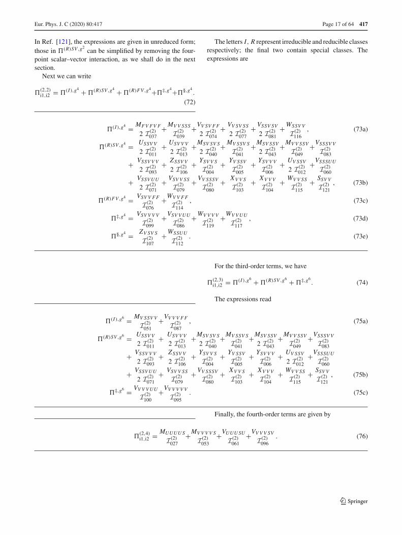
In Ref. [121], the expressions are given in unreduced form;those in �(R)SV,g2
can be simplified by removing the four-point scalar–vector interaction, as we shall do in the nextsection.
Next we can write
�(2,2)i1,i2 = �(I ),g4 + �(R)SV,g4 + �(R)FV,g4+�‡,g4+�§,g4
.
(72)
The letters I, R represent irreducible and reducible classesrespectively; the final two contain special classes. Theexpressions are
�(I ),g4 = MFV FV F
2 I(2)037
+MVV SSS
I(2)039
+VV SV FF
2 I(2)074
+ VV SV SS
2 I(2)077
+VSSV SV
2 I(2)081
+WSSVV
I(2)116
, (73a)
�(R)SV,g4 = USSVV
2 I(2)011
+ USVVV
2 I(2)013
+MSV SV S
2 I(2)040
+MVSSV S
I(2)041
+MSV SSV
2 I(2)043
+MVV SSV
I(2)049
+VSSSV V
I(2)083
+ VSSV VV
2 I(2)093
+ ZSSV V
2 I(2)106
+ YSVV S
I(2)004
+ YV SSV
I(2)005
+ YSVVV
I(2)006
+ UV SSV
2 I(2)012
+VSSSUU
I(2)060
+ VSSVUU
2 I(2)071
+ VSVV SS
I(2)079
+VV SSSV
I(2)080
+ XVV S
I(2)103
+ XVVV
I(2)104
+ WVV SS
I(2)115
+ SSVV
I(2)121
, (73b)
�(R)FV,g4 = VSVV FF
I(2)076
+WVV FF
I(2)114
, (73c)
�‡,g4 = VSVVVV
I(2)099
+VSVVUU
I(2)086
+WVVVV
I(2)119
+WVVUU
I(2)117
, (73d)
�§,g4 = ZV SV S
I(2)107
+WSSUU
I(2)112
. (73e)
For the third-order terms, we have
�(2,3)i1,i2 = �(I ),g6 + �(R)SV,g6 + �‡,g6
. (74)
The expressions read
�(I ),g6 = MVSSVV
I(2)051
+VVVV FF
I(2)087
, (75a)
�(R)SV,g6 = USSVV
2 I(2)011
+ USVVV
2 I(2)013
+MSV SV S
2 I(2)040
+MVSSV S
I(2)041
+MSV SSV
2 I(2)043
+MVV SSV
I(2)049
+VSSSV V
I(2)083
+ VSSV VV
2 I(2)093
+ ZSSV V
2 I(2)106
+ YSVV S
I(2)004
+ YV SSV
I(2)005
+ YSVVV
I(2)006
+ UV SSV
2 I(2)012
+VSSSUU
I(2)060
+ VSSVUU
2 I(2)071
+ VSVV SS
I(2)079
+VV SSSV
I(2)080
+ XVV S
I(2)103
+ XVVV
I(2)104
+ WVV SS
I(2)115
+ SSVV
I(2)121
, (75b)
�‡,g6 = VVVVUU
I(2)100
+VVVVVV
I(2)095
. (75c)
Finally, the fourth-order terms are given by
�(2,4)i1,i2 = MUUUUS
I(2)027
+MVVVV S
I(2)053
+VUUUSU
I(2)061
+VVVV SV
I(2)096
. (76)
123
417 Page 18 of 64 Eur. Phys. J. C (2020) 80 :417
Together, these describe 92 classes. However, we canimmediately reduce this to 89 by removing the ghost–ghost–vector couplings inside �‡,g4
and �‡,g6, as we describe in
the next sections.
4.2.2 Combination of classes
As in the case of the tadpole diagrams, we shall exchangefour-point couplings involving vectors, and all ghost cou-plings, for three-point couplings involving scalars and vec-tors. We therefore use the same notation as in the tadpolecase to represent our loop functions and their couplings; theself-energy diagrams can be written as
I(2)N =
∑
{L}f (l1,··· ,lm )N (i3, . . . , i(n + 2))
m∏
j=1
C[. . . , L j ]. (77)
In the cases where there is only one function, we omit thesuperscript with the Lorentz indices. For example, we canwrite
I(2)104 = SSVV[i1, i2, i3, i4, 1]VVVV[i3, i4, i5, i5, 1] f (1,1)
104 (i3, i4, i5)
+ SSVV[i1, i2, i3, i4, 1]VVVV[i3, i4, i5, i5, 2] f (1,2)104 (i3, i4, i5)
+ SSVV[i1, i2, i3, i4, 1]VVVV[i3, i4, i5, i5, 3] f (1,3)104 (i3, i4, i5),
(78)
but
I(2)001 = SSS[i1, i3, i4, 1]
SSS[i2, i3, i5, 1]SSSS[i4, i5, i6, i6, 1] f1(i3, i4, i5, i6). (79)
The first trivial application of this is to remove the dia-grams with ghosts that do not couple to scalars. In the abovenotation we can write
�‡,g6 = SVV[i1, i3, i4, 1]SVV[i2, i3, i7, 1]VVV[i4, i5, i6, 1]VVV[i5, i6, i7, 1]×
[f (1,1,1,1)100 (i3, i4, i5, i6, i7) − 4 f (1,1,1,1)
95 (i3, i4, i5, i6, i7)],
(80)
where we note that f (1,1,1,1)95 = f (1,1,2,2)
95 , and �‡,g4consists
of two classes corresponding to diagrams I(2)099 and I(2)
119 :
�‡,g4 = SSV[i1, i3, i4, 1]SSV[i2, i3, i7, 1]VVV[i4, i5, i6, 1]VVV[i5, i6, i7, 1]×
[f (1,1,1,1)99 (i3, i4, i5, i6, i7) − 4 f (1,1,1,1)
86 (i3, i4, i5, i6, i7)]
+ SSVV[i1, i2, i5, i6, 1]VVV[i3, i4, i5, 1]VVV[i3, i4, i6, 1]×
[f (1,1,1)119 (i3, i4, i5, i6) − 4 f (1,1,1)
117 (i3, i4, i5, i6)]. (81)
This reduces the number of classes of diagrams to evaluate to89, which will speed up evaluation (since the loop functionsare all of the same class, they require no substantial extra timeto evaluate, whereas performing loops over the couplings andevaluating the loop functions each time is slow). In fact, byusing Eq. (28) we can combine these two classes of diagramsinto one graph of topology VSVVVV ; but we shall apply thissystematically in the next section.
4.2.3 Ghostbusting
In the previous section we eliminated diagrams contain-ing only ghost–ghost–vector couplings and no ghost–ghost–scalar couplings. In this section we shall remove all ghostcouplings from the amplitude, and also apply Eq. (14) andEq. (28) in order to obtain only 58 classes to evaluate in total(compared to the 28 for up to O(g2) terms) at the expense ofrequiring that the external scalars are notwould-beGoldstonebosons.
The key equation that we shall apply is Eq. (44) whichshows how we can relate SUU couplings to scalar and vectorcouplings. However, the form of those couplings has an extracontribution for would-be Goldstone bosons:
SUU[i1,−i2, i3, 1] = −ξ
2SVV[i1, i2, i3, 1]
− ı
2
∑
i4
ξ (FD)i4i1 VVV[i4, i2, i3, 1]. (82)
We therefore have to make some distinction betweenwould-be Goldstone bosons and the other scalars in the sum-mation. One approach to dealing with this would be to intro-duce the Goldstone bosons as a new class of fields (separatefrom other scalars) from the start, and remove them via theidentities in Sect. 3 afterwards. This would be necessary toobtain an explicitly gauge-invariant result, and should lead toa faster evaluation of the final result, but comes at the expenseof complicating the expressions. We leave this to future work.
Instead, we deal with the above problem by noting thatthe first term on the right-hand side of Eq. (82) is universalfor all scalars whether they are Goldstone bosons or not,so we can split any diagram containing an SUU vertex intotwo (or more) and explicitly sum over the second part, sinceit effectively becomes a vector propagator. As an example,consider I(2)
027:
I(2)027 = SUU[i1,−i3, i6, 1]SUU[i2,−i7, i4, 1]
SUU[i5,−i4, i3, 1]SUU[i5,−i6, i7, 1] f27(i3, i4, i5, i6, i7)
= SVV[i1, i3, i6, 1]SVV[i2, i4, i7, 1]SVV[i5, i3, i4, 1]SVV[i5, i6, i7, 1] 1
8f27(i3, i4, i5, i6, i7)
123

Eur. Phys. J. C (2020) 80 :417 Page 19 of 64 417
+ SVV[i1, i3, i6, 1]SVV[i2, i4, i7, 1]VVV[i3, i4, i5, 1]VVV[i5, i6, i7, 1] 1
8m2i5 f27(i3, i4, i5, i6, i7).
(83)
Two combinations here have dropped out:
ı
8mi5 f27(i3, i4, i5, i6, i7)
[SVV[i1, i3, i6, 1]SVV[i2, i4, i7, 1]
SVV[i5, i3, i4, 1]VVV[i5, i6, i7, 1]+SVV[i1, i3, i6, 1]SVV[i2, i4, i7, 1]VVV[i5, i3, i4, 1]SVV[i5, i6, i7, 1]
]= 0 , (84a)
ı
8mi5 f27(i4, i3, i5, i7, i6)
[SVV[i2, i4, i7, 1]SVV[i1, i3, i6, 1]
SVV[i5, i4, i3, 1]VVV[i5, i7, i6, 1]+SVV[i2, i4, i7, 1]SVV[i1, i3, i6, 1]VVV[i5, i4, i3, 1]SVV[i5, i7, i6, 1]
]= 0. (84b)
Schematically we then have
and we see that the diagrams that drop out would not havefit with the above picture (note that almost exactly the samepattern reproduces for diagram I(2)
061 ). In the diagram on theleft, the sum over scalar propagators is indeed a sum over allscalars in the theory. We restrict to the case that the externalstates are not Goldstone bosons here, because otherwise thecouplings for the diagrams on the right hand side of the aboverelations would include gauge bosons as external legs, andwe would therefore need to combine those amplitudes withmixed scalar–vector and vector–vector amplitudes.
There are also complications when the “Goldstone” legattaches to a triple or quartic scalar vertex. The reason forthis can be traced back to Eq. (52): masses appear in theGSS coupling relation that are different for Goldstone bosonsthan for other scalars (in any gauge except Landau gauge),and this then feeds into the relation for the GSSS coupling.There would also potentially be a similar problem for theSGV vertex, but in all our examples this is avoided becausewe assert that we have no external Goldstone bosons. There isonly one diagram with a quartic scalar coupling and ghosts –I(2)
112 – that we will discuss in more detail below, but diagrams
I(2)025 , I(2)
060 and I(2)071 contain triple scalar couplings, that we
treat by using Eq. (55) and again splitting the diagram into
sums over all scalars and sums over just Goldstone indices,explicitly trading the Goldstone bosons for vectors.
4.2.4 Final simplified results for self-energies
The final result for our set of 58 self-energy topologies canbe expressed as:
�(2,0)i1,i2 = �S + �SF , (85a)
�(2,1)i1,i2 = �(I )SV,g2 + �(I )SFV,g2 + �
SV,g2
, (85b)
�(2,2)i1,i2 = �(I ),g4 + �
FV,g4 + �SUV,g4 + �§,g4
, (85c)
�(2,3)i1,i2 = �(I ),g6 + �
g6
, (85d)
�(2,4)i1,i2 = �
g8
. (85e)
The pieces without bars are unchanged from above, the oneswith bars are explained in the following.
4.2.5 Reduced diagrams of O(g2)
The combined diagrams start at O(g2):
�SV,g2 = SSS[i1, i3, i4, 1]SSS[i2, i3, i7, 1]SSV[i4, i5, i6, 1]SSV[i5, i7, i6, 1]×
{f69(i3, i4, i5, i6, i7) − f2(i3, i4, i7, i6) − f2(i3, i7, i4, i6)
}
+ SSSS[i1, i2, i5, i6, 1]SSV[i3, i5, i4, 1]SSV[i3, i6, i4, 1]×
{f113(i3, i4, i5, i6) + 2 f102(i5, i6, i4)
}. (86)
4.2.6 Reduced diagrams of O(g4)
The only new diagrams with fermions enter at order O(g4)
and are given by:
�FV,g4
= 2 e[FFV[i5, i6, i4, 1]FFV[i5, i6, i7, 1]SSV[i1, i3, i4, 1]SSV[i2, i3, i7, 1]]×
{f (1,1,1,1)76 (i3, i4, i5, i6, i7) + 2 f (1,1,1)
114 (i5, i6, i4, i7)}
123

417 Page 20 of 64 Eur. Phys. J. C (2020) 80 :417
+ 2 e[FFV[i5, i6, i4, 1]FFV[i5, i6, i7, 2]SSV[i1, i3, i4, 1]SSV[i2, i3, i7, 1]]×
{f (1,2,1,1)76 (i3, i4, i5, i6, i7) + 2 f (1,2,1)
114 (i5, i6, i4, i7)}. (87)
The other combined diagrams at order O(g4) are:
�SUV,g4 = MSV SSV + MSV SV S + MVSSV S + MVV SSV
+ V SSSV V + V SVV SS + V SVVVV + V V SSSV .
(88)
These new topologies are:
MSV SSV = SSS[i1, i3, i6, 1]SSV[i2, i4, i7, 1]SSV[i3, i4, i5, 1]SVV[i6, i5, i7, 1]×
{2 f43(i3, i4, i5, i6, i7) + 4 f11(i6, i5, i7, i3)
},
(89a)
MSV SV S = SSS[i1, i3, i6, 1]SSV[i3, i5, i4, 1]SSV[i5, i6, i7, 1]SVV[i2, i4, i7, 1]×
{2 f40(i3, i4, i5, i6, i7) − 4 f106(i3, i6, i4, i7)
},
(89b)
MVSSV S = SSV[i1, i3, i6, 1]SSV[i2, i7, i4, 1]SSV[i3, i5, i4, 1]SSV[i5, i7, i6, 1]×
{f41(i3, i4, i5, i6, i7) + f12(i3, i5, i4, i6)
+ f12(i7, i5, i6, i4) − 2 f121(i5, i4, i6)}
, (89c)
MVV SSV = SSV[i1, i3, i6, 1]SSV[i2, i4, i7, 1]SSV[i3, i4, i5, 1]VVV[i5, i6, i7, 1]×
{f49(i3, i4, i5, i6, i7) − 2 f13(i6, i5, i7, i3)
− 2 f13(i7, i5, i6, i4)}
, (89d)
V SSSV V = SSS[i1, i3, i4, 1]SSS[i2, i3, i7, 1]SVV[i4, i5, i6, 1]SVV[i7, i5, i6, 1]×
{f83(i3, i4, i5, i6, i7) + 1
2f60(i3, i4, i5, i6, i7)
},
(89e)
V SVV SS = SSV[i1, i3, i4, 1]SSV[i2, i3, i7, 1]SSV[i5, i6, i4, 1]SSV[i5, i6, i7, 1]×
{f79(i3, i4, i5, i6, i7) + 2 f115(i5, i6, i4, i7)
+ 2 f103(i4, i7, i5) + 2 f103(i4, i7, i6)
+ 1
2
[f4(i3, i4, i7, i5) + f4(i3, i4, i7, i6)
+ f4(i3, i7, i4, i5) + f4(i3, i7, i4, i6)]}
, (89f)
V SVVVV = SSV[i1, i3, i4, 1]SSV[i2, i3, i7, 1]
VVV[i4, i5, i6, 1]VVV[i5, i6, i7, 1]×
{f99(i3, i4, i5, i6, i7) + 2 f119(i5, i6, i4, i7)
− 1
2
(m2
i1 − m2i3
) (m2
i2 − m2i3
)f60(i3, i4, i5, i6, i7)
+ 1
4
(m2
i1 + m2i2 − 2m2
i3
)
[f71(i3, i4, i5, i6, i7) + f71(i3, i4, i6, i5, i7)
]
− f (1,1,1)6 (i3, i4, i7, i5) − f (1,1,1)
6 (i3, i4, i7, i6)
+ f (1,1,3)6 (i3, i4, i7, i5) + f (1,1,3)
6 (i3, i4, i7, i6)
− 2 f86(i3, i4, i5, i6, i7) − 4 f117(i3, i4, i5, i6, i7)
− 2 f (1,1)104 (i4, i7, i5) − 2 f (1,1)
104 (i4, i7, i6)
+ 2 f (1,3)104 (i4, i7, i5) + 2 f (1,3)
104 (i4, i7, i6)
}, (89g)
V V SSSV = SSV[i1, i4, i3, 1]SSV[i2, i7, i3, 1]SSV[i4, i5, i6, 1]SSV[i5, i7, i6, 1]×
{f80(i3, i4, i5, i6, i7)
− f5(i3, i4, i7, i6) − f5(i3, i7, i4, i6)
− 2 f121(i5, i3, i6) + f12(i4, i5, i6, i3)
+ f12(i7, i5, i6, i3)}. (89h)
4.2.7 Reduced diagrams of O(g6)
The 10 combined diagrams involving scalar and vector cou-plings of O(g6) are given by
�g6 = MSV SVV + MVV SV S + MVV SVV + MVVVVV
+ V SVV SV + V V SSV V + V V SV SV
+ V V SVVV + V VVV SS + V VVVVV . (90)
The topologies of type “M” are:MSV SVV = SSS[i1, i3, i6, 1]SVV[i2, i4, i7, 1]
SVV[i3, i4, i5, 1]SVV[i6, i5, i7, 1]×
{2 f50(i3, i4, i5, i6, i7) − 1
2f25(i3, i4, i5, i6, i7)
},
(91a)
MVV SV S = SSV[i1, i3, i6, 1]SSV[i3, i5, i4, 1]SVV[i2, i4, i7, 1]SVV[i5, i6, i7, 1]×
{2 f47(i3, i4, i5, i6, i7) − 2 f14(i7, i5, i6, i4)
}, (91b)
MVV SVV = SSV[i1, i3, i6, 1]SVV[i2, i4, i7, 1]SVV[i3, i4, i5, 1]VVV[i5, i6, i7, 1]×
{2 f54(i3, i4, i5, i6, i7) − 1
2f (1,1,1,1)34 (i3, i4, i5, i6, i7)
123
Eur. Phys. J. C (2020) 80 :417 Page 21 of 64 417
+1
2f (1,1,1,2)34 (i3, i4, i5, i6, i7)
}, (91c)
MVVVVV = SVV[i1, i3, i6, 1]SVV[i2, i4, i7, 1]VVV[i3, i4, i5, 1]VVV[i5, i6, i7, 1]×
{f56(i3, i4, i5, i6, i7)
+ 1
8
(m2
i1 + m2i2
)f25(i3, i4, i5, i6, i7)
− 2 f (1,1,1)109 (i3, i6, i4, i7) + 2 f (1,1,3)
109 (i3, i6, i4, i7)
+ 1
8m2
i5 f27(i3, i4, i5, i6, i7)
− 1
16
[f (1,1,1,1)34 (i3, i4, i5, i6, i7) + f (1,1,1,2)
34 (i3, i4, i5, i6, i7)
+ f36(i3, i4, i5, i6, i7)
+ f (1,1,1,1)34 (i4, i3, i5, i7, i6) + f (1,1,1,2)
34 (i4, i3, i5, i7, i6)
+ f36(i4, i3, i5, i7, i6)
+ f (1,1,1,1)34 (i6, i7, i5, i3, i4) + f (1,1,1,2)
34 (i6, i7, i5, i3, i4)
+ f36(i6, i7, i5, i3, i4)
+ f (1,1,1,1)34 (i7, i6, i5, i4, i3) + f (1,1,1,2)
34 (i7, i6, i5, i4, i3)
+ f36(i7, i6, i5, i4, i3)]
+ 1
4
[f45(i3, i4, i5, i6, i7) + f45(i4, i3, i5, i7, i6)
+ f45(i6, i7, i5, i3, i4) + f45(i7, i6, i5, i4, i3)]}
. (91d)
The last term in the above appears fearsome, but actually itsfinite part simplifies dramatically:
Fin[MVVVVV
] = SVV[i1, i3, i6, 1]SVV[i2, i4, i7, 1]VVV[i3, i4, i5, 1]VVV[i5, i6, i7, 1]×
{δMS
[5 − 9
4B(m2
i3,m2i6) − 9
4B(m2
i4,m2i7)
+15
8B(m2
i3,m2i6) B(m2
i4,m2i7)
]
+ 1
16
[34m2
i3 + 34m2i4 + 34m2
i6 + 34m2i7
+65m2i5 − 66 p2 − m2
i1 − m2i2
]
× M(m2i3,m
2i7,m
2i6,m
2i4,m
2i5)
− 17
8U (m2
i3,m2i6,m
2i5,m
2i7)
− 17
8U (m2
i4,m2i7,m
2i5,m
2i6)
− 17
8U (m2
i6,m2i3,m
2i4,m
2i5)
− 17
8U (m2
i7,m2i4,m
2i3,m
2i5)
}. (92)
This expression is untroubled if any masses are coincidentor vanishing.
The topologies of type “V ” are:
V SVV SV = SSV[i1, i3, i4, 1]SSV[i2, i3, i7, 1]SVV[i5, i4, i6, 1]SVV[i5, i6, i7, 1]×
{f91(i3, i4, i5, i6, i7) + 2 f118(i5, i6, i4, i7)
},
(93a)
V V SSV V = SSV[i1, i4, i3, 1]SSV[i2, i7, i3, 1]SVV[i4, i5, i6, 1]SVV[i7, i5, i6, 1]×
{f92(i3, i4, i5, i6, i7) + 1
2f70(i3, i4, i5, i6, i7)
},
(93b)
V V SV SV = SSV[i1, i4, i3, 1]SSV[i4, i5, i6, 1]SVV[i2, i3, i7, 1]SVV[i5, i6, i7, 1]×
{2 f89(i3, i4, i5, i6, i7) − 2 f14(i7, i5, i6, i3)
},
(93c)
V V SVVV = SSV[i1, i4, i3, 1]SVV[i2, i3, i7, 1]SVV[i4, i5, i6, 1]VVV[i5, i6, i7, 1]×
{2 f97(i3, i4, i5, i6, i7) + 1
2f84(i3, i4, i5, i6, i7)
−1
2f84(i3, i4, i6, i5, i7)
}. (93d)
V VVV SS = SSV[i5, i6, i4, 1]SSV[i5, i6, i7, 1]SVV[i1, i3, i4, 1]SVV[i2, i3, i7, 1]×
{f88(i3, i4, i5, i6, i7) + f7(i3, i4, i7, i5)
+ f7(i3, i4, i7, i6)}
, (93e)
VVVVVV = SVV[i1, i3, i4, 1]SVV[i2, i3, i7, 1]VVV[i4, i5, i6, 1]VVV[i5, i6, i7, 1]×
{f100(i3, i4, i5, i6, i7) − 2 f95(i3, i4, i5, i6, i7)
− 1
8f70(i3, i4, i5, i6, i7)
− f (1,1,1)8 (i3, i4, i7, i5) − f (1,1,1)
8 (i3, i4, i7, i6)
+ f (1,1,3)8 (i3, i4, i7, i5) + f (1,1,3)
8 (i3, i4, i7, i6)
− m2i3
8
(
1 − m2i1
m2i4
− m2i2
m2i7
)
f60(i3, i4, i5, i6, i7)
+ 1
16
(m2
i5 + m2i6
)f61(i3, i4, i5, i6, i7)
− 1
8
[f71(i3, i4, i5, i6, i7) + f71(i3, i4, i6, i5, i7)
]
+ 1
4
[f84(i3, i4, i5, i6, i7) + f84(i3, i4, i6, i5, i7)
− f73(i3, i4, i5, i6, i7) − f73(i3, i4, i6, i5, i7)]}
.
(93f)
123

417 Page 22 of 64 Eur. Phys. J. C (2020) 80 :417
For the last expression, the factors of m2i4 and m2
i7 in thedenominators may at first appear to lead to divergencesif the corresponding gauge bosons are massless. However,it is straightforward to show that, in that case and fori1, i2 not would-be Goldstone bosons, the SVV[i1, i3, i4, 1],SVV[i2, i3, i7, 1] vertices also vanish. This expression simpli-fies to a relatively short form similarly to MVVVVV , exceptthat the reduction is different for m2
i4 = m2i7 as compared to
the non-degenerate case.
4.2.8 Reducible diagrams containing scalars and vectorsof O(g8)
The nominally highest-order diagrams in the gauge couplingconsist of just two topologies, reduced from the original four:
�g8 = MVVVV S + V VVV SV . (94)
The expressions for these are:
MVVVV S = SVV[i1, i3, i6, 1]SVV[i2, i4, i7, 1]SVV[i5, i3, i4, 1]SVV[i5, i6, i7, 1]×
{f53(i3, i4, i5, i6, i7) + 1
8f27(i3, i4, i5, i6, i7)
},
(95a)
V VVV SV = SVV[i1, i3, i4, 1]SVV[i2, i3, i7, 1]SVV[i5, i4, i6, 1]SVV[i5, i6, i7, 1]×
{f96(i3, i4, i5, i6, i7) + 1
8f61(i3, i4, i5, i6, i7)
}.
(95b)
4.2.9 Special topologies: �§,g4
Recall that �§,g4 = I(2)107+I(2)
112. These two diagrams containreducible couplings; the first has a four-point scalar–vectorcoupling, and the second contains ghosts. However, whenwe remove the four-point vector–scalar interactions and theghosts we find topologies that are either not 1PI or containinternal propagators. The first of these is I(2)
107 :
I(2)107 = SSV[i1, i3, i4, 1]SSV[i2, i5, i6, 1]
SSVV[i3, i5, i4, i6, 1] f107(i3, i4, i5, i6)
= −SSV[i1, i3, i6, 1]SSV[i2, i7, i4, 1]SSV[i3, i5, i4, 1]SSV[i5, i7, i6, 1] f107(i3, i6, i7, i4)
+ SSV[i1, i3, i4, 1]SSV[i2, i5, i6, 1]SSV[i3, i7, i4, 1]SSV[i5, i7, i6, 1] f107(i3, i4, i5, i6). (96)
The first diagram contributes to topology MV SSV S or I(2)041 ,
while the second is a non-1PI diagram; schematically:
The second interesting topology is I(2)112 :
I(2)112 = SSSS[i1, i2, i5, i6, 1]SUU[i5,−i4, i3, 1]
SUU[i6,−i3, i4, 1] f112(i3, i4, i5, i6)
= 1
2
(m2
i1 + m2i2 − 2m2
i3
)SSV[i1, i3, i4, 1]
SSV[i2, i3, i7, 1]VVV[i4, i5, i6, 1]VVV[i5, i6, i7, 1]f112(i5, i6, i4, i7)
− 1
8SVV[i1, i3, i4, 1]SVV[i2, i3, i7, 1]
VVV[i4, i5, i6, 1]VVV[i5, i6, i7, 1] f112(i5, i6, i4, i7)
+ 1
2SSSS[i1, i2, i5, i6, 1]SVV[i5, i3, i4, 1]
SVV[i6, i3, i4, 1] f112(i5, i6, i4, i7)
− 1
4SSS[i1, i2, i7, 1]SVV[i7, i5, i6, 1]
VVV[i3, i4, i5, 1]VVV[i3, i4, i6, 1] f112(i3, i4, i5, i6). (97)
Here we have used Eq. (54) and substituted Eq. (55) intoEq. (56). The topologies on the right-hand side correspondto I(2)
099 (VSVVVV ), I(2)100 (VVVVVV ), I(2)
116 (WSSVV ) andan extra diagram, schematically:
123
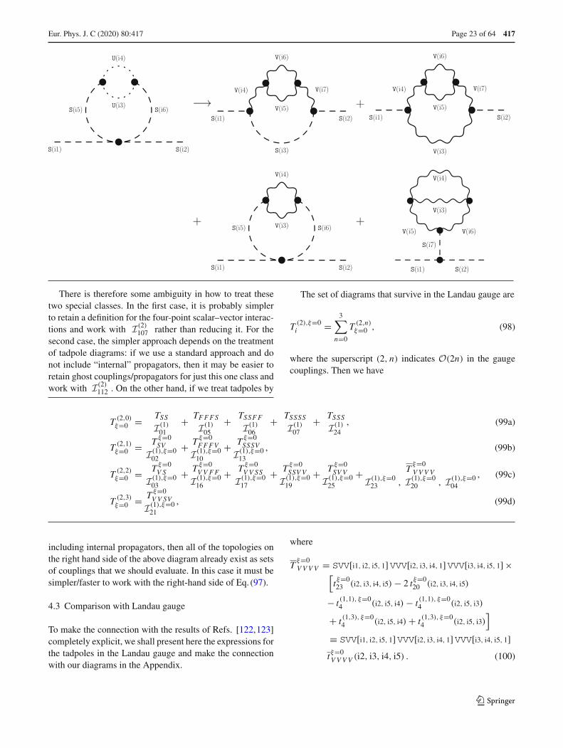
Eur. Phys. J. C (2020) 80 :417 Page 23 of 64 417
There is therefore some ambiguity in how to treat thesetwo special classes. In the first case, it is probably simplerto retain a definition for the four-point scalar–vector interac-tions and work with I(2)
107 rather than reducing it. For thesecond case, the simpler approach depends on the treatmentof tadpole diagrams: if we use a standard approach and donot include “internal” propagators, then it may be easier toretain ghost couplings/propagators for just this one class andwork with I(2)
112 . On the other hand, if we treat tadpoles by
including internal propagators, then all of the topologies onthe right hand side of the above diagram already exist as setsof couplings that we should evaluate. In this case it must besimpler/faster to work with the right-hand side of Eq. (97).
4.3 Comparison with Landau gauge
To make the connection with the results of Refs. [122,123]completely explicit, we shall present here the expressions forthe tadpoles in the Landau gauge and make the connectionwith our diagrams in the Appendix.
The set of diagrams that survive in the Landau gauge are
T (2),ξ=0i =
3∑
n=0
T (2,n)ξ=0 , (98)
where the superscript (2, n) indicates O(2n) in the gaugecouplings. Then we have
T (2,0)ξ=0 = TSS
I(1)01
+ TFFFS
I(1)05
+ TSSFF
I(1)06
+ TSSSSI(1)
07+ TSSS
I(1)24
, (99a)
T (2,1)ξ=0 = T ξ=0
SV
I(1),ξ=002
+ T ξ=0FFFV
I(1),ξ=010
+ T ξ=0SSSV
I(1),ξ=013
, (99b)
T (2,2)ξ=0 = T ξ=0
V S
I(1),ξ=003
+ T ξ=0VV FF
I(1),ξ=016
+ T ξ=0VV SS
I(1),ξ=017
+ T ξ=0SSV V
I(1),ξ=019
+ T ξ=0SV V
I(1),ξ=025
+ Tξ=0VVVV
I(1),ξ=023 , I(1),ξ=0
20 , I(1),ξ=004
, (99c)
T (2,3)ξ=0 = T ξ=0
VV SV
I(1),ξ=021
, (99d)
where
Tξ=0VVVV = SVV[i1, i2, i5, 1]VVV[i2, i3, i4, 1]VVV[i3, i4, i5, 1] ×
[tξ=023 (i2, i3, i4, i5) − 2 tξ=0
20 (i2, i3, i4, i5)
− t (1,1), ξ=04 (i2, i5, i4) − t (1,1), ξ=0
4 (i2, i5, i3)
+ t (1,3), ξ=04 (i2, i5, i4) + t (1,3), ξ=0
4 (i2, i5, i3)]
≡ SVV[i1, i2, i5, 1]VVV[i2, i3, i4, 1]VVV[i3, i4, i5, 1]tξ=0VVVV (i2, i3, i4, i5) . (100)
123

417 Page 24 of 64 Eur. Phys. J. C (2020) 80 :417
The topologies (and therefore labelling of the couplings)are the same in Landau gauge as for our Feynman-gaugeresults in the Appendix, but we add the superscript ξ = 0here. We do not give the explicit expressions for these, sinceseveral are rather long – they contain many more integralsthan the Feynman-gauge case – but they are provided as partof TLDR.
Ignoring for the moment cases where some masses vanish,and using the loop functions defined in Ref. [119] and thenotation
Dx,y[ f (x)] ≡ f (x) − f (y)
x − y, (101a)
Dx,x [ f (x)] ≡ limy→x
Dx,y[ f (x)], (101b)
we find the following expressions for the tadpoles:
Tadpole topology Label Finite Part Our function
I(1)01 T ξ=0
SS − 14 a(i1)i j λi jkk Dm2
i ,m2j
[fSS(m2
i ,m2k)
]a(i1)i j λi jkk t1(i, k, j)
I(1)24 T ξ=0
SSS − 16 λ(i1)i jk ai jk fSSS(m2
i ,m2j ,m
2k) λ(i1)i jk ai jk t24(i, j, k)
I(1)07 T ξ=0
SSSS − 14 a(i1)i j aikl a jkl Dm2
i ,m2j
[fSSS(m2
i ,m2k ,m
2l )
]a(i1)i j aikl a jkl t7(i, k, l, j)
I(1)02 T ξ=0
SV − 14 aik(i1) gaaik Dm2
i ,m2k
[fV S(m2
a,m2i )
] −aik(i1) gaaik tξ=02 (i, k, a)
I(1)03 T ξ=0
V S − 14 gabii gab(i1) Dm2
a ,m2b
[fV S(m2
a,m2i )
]gabii gab(i1) tξ=0
3 (a, b, i)
I(1)13 T ξ=0
SSSV − 12 aik(i1) gai j gak j Dm2
i ,m2k
[fSSV (m2
i ,m2j ,m
2a)
]aik(i1) gai j gak j tξ=0
13 (i, j, a, k)
I(1)17 T ξ=0
VV SS − 14 gab(i1) gai j gbi j Dm2
a ,m2b
[fSSV (m2
i ,m2j ,m
2a)
]gab(i1) gai j gbi j tξ=0
17 (a, i, j, b)
I(1)19 T ξ=0
SSV V − 14 gabi gabj ai j (i1) Dm2
i ,m2j
[fV V S(m2
a,m2b,m
2i )
]gabi gabj ai j (i1) tξ=0
19 (i, a, b, j)
I(1)25 T ξ=0
SV V − 12 gabi(i1) gabi fV V S(m2
a,m2b,m
2i ) gabi(i1) gabi tξ=0
25 (i, a, b)
I(1)21 T ξ=0
VV SV − 12 gabi gcbi gac(i1) Dm2
a ,m2c
[fV V S(m2
a,m2b,m
2i )
] −gabi gcbi gac(i1) tξ=021 (a, i, b, c)
I(1)23 , I(1)
20 , I(1)04 T
ξ=0VVVV − 1
4 gabc gdbc gad(i1) Dm2a ,m
2d
[fgauge(m2
a,m2b,m
2c)
]gabc gdbc gad(i1) tξ=0
VVVV (a, b, c, d)
The fermionic diagrams are:
Fin[T ξ=0FFFV
]= 2 gaJI gKbJ e
[MK I ′ y I
′ I (i1)]
Dm2I ,m
2K
[fFFV (m2
I ,m2J ,m
2a)
]
+ gaJI gaJ′
I ′ e[y I I
′(i1) M∗J J ′
]
[fFFV (m2
I ,m2J ,m
2a)
+m2I Dm2
I ,m2I ′
[fFFV (m2
I ,m2J ,m
2a)
]]
+ gaJI gaJ′
I ′ e[MIK ′
MK I ′M∗
J J ′ yK K ′(i1)
]
Dm2I ,m
2I ′
[fFFV (m2
I ,m2J ,m
2a)
], (102a)
Fin[T ξ=0VV FF
]= 1
2gaJI gIbJ g
ab(i1)
Dm2a ,m
2b
[fFFV (m2
I ,m2J ,m
2a)
]
+ 1
2gaJI gbJ
′I ′ gab(i1) MI I ′
M∗J J ′
Dm2a ,m
2b
[fFFV (m2
I ,m2J ,m
2a)
]. (102b)
In Refs. [122,123] the topology T ξ=0SV V was missing. Our new
approach, however, pays immediate dividends when we con-sider some masses to be vanishing. We find, for example, that
t1(0, k, 0) = 0, (103a)
Fin[t7(0, k, l, 0)] = −1
4RSS(m
2k,m
2l ) + 1
4B
∣∣ε1
0
(0,m2
k,m2l
),
(103b)
where RSS(x, y) is defined in Refs. [123,136]; using theexpressions in the Appendix we can find the finite part of allof the integrals even in the case of vanishing masses. Thesecond term on the right-hand side of Eq. (103b) clearly
arises from an infra-red divergence; such divergences are thecounterparts of the expansions found in Ref. [123], wherethe equivalent for Eq. (103b) is
Dm2G ,m2
G
[fSSS(m
2G ,m2
k,m2l )
]= RSS(m
2k,m
2l )
− B∣∣ε0
0
(0,m2
k,m2l
)log
m2G
Q2 + O(m2G
)(104)
with the renormalisation scale Q. Instead of an expansion inthe mass of the Goldstone bosons, we use dimensional reg-ularisation in order to regularise the infra-red divergences.Then we should find that the infra-red divergent parts inthe two-loop calculation cancel exactly against equivalentparts coming either from putting the Goldstone-boson masseson-shell in the one-loop parts, or using “consistent tadpolesolutions” (by using tree-level masses in the one-loop cal-culation). We intend to elaborate further on this connectionelsewhere.
123

Eur. Phys. J. C (2020) 80 :417 Page 25 of 64 417
4.4 Standard Model calculation
Our self-energies up to second order in the gauge couplinghave been compared with the expressions in Ref. [121], and,as we have shown above, the tadpoles in the Landau gaugeexactly match those found in Ref. [122]. In order to explicitlycross-check our Feynman-gauge result, and the combinationsof classes, it would be desirable to have models to compare to.However, as described in the introduction, the only examplewhere scalar electroweak corrections have been computed isfor the Higgs mass in the Standard Model. Since the resultsare very long, these have been made public in the form ofcomputer codes SMH [17], mr [18,19] and SMDR [25].
The result used in mr has been computed including tad-poles via internal propagators in a general gauge, and is excel-lent for a numerical calculation. However, the expressions inSMH are actually written in a sufficiently convenient form tobe translated into code readable by Mathematica, and sowe were able to use it for an analytical cross-check of ourresults. On the other hand, the result there is in Landau gauge,and combines the tadpoles with self-energy contributions viaEq. (7).
Therefore we have cross-checked our results against theStandard Model by the following procedure:
• We calculated the tadpoles and Higgs self-energies inthe Landau gauge using the FeynArts model file forthe SM (with some modifications that will be describedelsewhere), and using TwoCalc, TARCER and our ownreduction to reduce the basis of integrals to those that canbe evaluated by TSIL. We compared the analytic expres-sions with those in SMH and found perfect agreement inall terms. For this calculation we computed self-energiesand counterterms separately, rather than using the BPHZmethod (in the SM all necessary counterterms can bereduced to just evaluating two-point functions since thereare sufficiently many tree-level relationships among theparameters).
• Using the same method, we performed the same calcu-lation in Feynman gauge. The results differ from SMHonly by the treatment of tadpole diagrams once we takep2 equal to the tree-level Higgs mass. This leads to 899self-energy diagrams based on the initial 121 genericclasses in FeynArts, and 75 one-loop self-energy dia-grams with one-loop counterterm insertions (plus 161tadpoles and 25 one-loop tadpoles with one-loop coun-terterm insertions).
• We performed the same calculation using only the topolo-gies of our 58 combined classes with the combined loopfunctions as given in this section. This yielded only 425self-energy diagrams (and, of course, includes the coun-terterm contributions). Upon reducing to the TSIL basis
we find exact agreement of all termswith the above “bruteforce” approach.
5 Conclusions
We have given expressions for scalar self-energies and tad-poles at the complete two-loop order in Feynman gauge. Withthe aim of being flexible, we have given the results for allrenormalised component diagrams, and also a much shorterversion where the diagrams are combined into just 16 tad-pole and 58 self-energy topologies, provided that the externalscalars are not (would-be) Goldstone bosons. The results areprovided in the most compact analytical form that we couldgive, but are also available electronically as a new packageTLDR at http://tldr.hepforge.org (where more tools and cal-culations will be added over time) so that they can be easilyapplied. We also include online all of the replacement rulesand degeneracies for each diagram with routines for extract-ing the finite part.
This work closes a gap in the literature that has existed forat least sixteen years. However, thanks to the technology andtechniques that we have developed, it is just the first step ina new program of completing the electroweak corrections ingeneric theories. The logical next step is an implementationin a general code such as SARAH so that they can be appliedto any model automatically. The following steps are:
1. Gauge-boson and mixed gauge–scalar self-energies. Inparticular, the latter are required for decay processes,while the former are essential for the extraction of elec-troweak parameters.
2. Threshold corrections to match general theories onto theStandard Model via a pole-matching technique. Naivelythis requires matching gauge-boson masses, but as shownin Ref. [103] we only need the derivatives of the scalarself-energies, and gauge threshold corrections at zeroHiggs expectation value.
3. Muon decay in general theories. This is required forextraction of the Higgs electroweak expectation valuein fixed-order calculations. It is a four-point fermionamplitude, so is combinatorially much more complicatedthan two-point functions, but since it is at zero externalmomentum we do not have any new problems related toγ5, and the loop functions all reduce to the same onesused in the tadpoles.
4. Fermion self-energies, in particular to calculate the top-quark mass.
We have applied our results to the Standard Model andcompared to the existing expressions in the literature, find-ing perfect agreement. However, since the only analyticallyavailable calculation was performed in Landau gauge, it was
123
417 Page 26 of 64 Eur. Phys. J. C (2020) 80 :417
not possible to compare our Feynman-gauge calculation withan independent check. However, by combining the diagramswith all tadpole diagrams it should be possible to give anexplicitly gauge-independent result that could also be com-pared with mr. Moreover, using the results from Sect. 3 itshould also be possible to implicitly sum over all Goldstone-boson propagators in our general result, transforming theircouplings and masses into those of gauge bosons. We leavethese developments to future work.
Acknowledgements Both authors acknowledge support from the grant“HiggsAutomator” of the Agence Nationale de la Recherche (ANR)(ANR-15-CE31-0002), and the LABEX Institut Lagrange de Paris. Thework of SP was supported in part by BMBF Grant no. 05H18PACC2.MDG thanks Benjamin Fuks for sharing some helpful private code forthe calculation of counterterms.
Data Availability Statement This manuscript has associated data ina data repository. [Authors’ comment: This manuscript has associateddata in a data repository at http://tldr.hepforge.org.]
Open Access This article is licensed under a Creative Commons Attri-bution 4.0 International License, which permits use, sharing, adaptation,distribution and reproduction in any medium or format, as long as yougive appropriate credit to the original author(s) and the source, pro-vide a link to the Creative Commons licence, and indicate if changeswere made. The images or other third party material in this articleare included in the article’s Creative Commons licence, unless indi-cated otherwise in a credit line to the material. If material is notincluded in the article’s Creative Commons licence and your intendeduse is not permitted by statutory regulation or exceeds the permit-ted use, you will need to obtain permission directly from the copy-right holder. To view a copy of this licence, visit http://creativecommons.org/licenses/by/4.0/.Funded by SCOAP3.
Appendix
A Integral relations
In this appendix, we introduce the notation for the integralsthat are used in the list of results for tadpoles and self-energiesin Appx. B. After mentioning some general relations amongthese integrals, the reduction rules that are necessary in thisarticle are displayed. Finally, the UV-divergent parts of thebasic set of scalar integrals are given.
A.1 Notation and symmetries
We mostly follow the notation of Ref. [129],
Ti1···in =∫
ddq1 ddq2[ı π2 (2 π μ)d−4]2
1(k2i1
− m2i1
)· · ·
(k2in
− m2in
) ,
(105a)
Y [ j1··· jo]i1···in =
∫ddq1 ddq2
[ı π2 (2 π μ)d−4]2
k2j1
· · · k2jo(
k2i1
− m2i1
)· · ·
(k2in
− m2in
) ,
(105b)
with the indices i1, . . . , in, j1, . . . , jo ∈ {1, 2, 3, 4, 5}, thedimension d = 4 − 2 ε with the ultra-violet regulator ε, thedimensional regulator μ, and the kinematic variables
k1 = q1 , k2 = q1 + p , k3 = q2 − q1 ,
k4 = q2 , k5 = q2 + p (106)
that depend on the loop momenta q1, q2 and the externalmomentum k6 ≡ p. In addition, we use sub-indices a and bin order to distinguish denominators of the same kinematictype, but with possibly different masses.
The set of different two-point integrals can be reduced byusing shift and mirror symmetries of the loop momenta (seeRef. [129]). They can be applied by exchanging the indicesof the kinematic variables in the integrals in the followingways,
1 ↔ 2 and 4 ↔ 5 , 1 ↔ 4 and 2 ↔ 5 ,
1 ↔ 5 and 2 ↔ 4 , (107a)
1 ↔ 3 if 2 absent , 2 ↔ 3 if 1 absent ,
3 ↔ 4 if 5 absent , 3 ↔ 5 if 4 absent , (107b)
1 ↔ 2 if 3 absent , 4 ↔ 5 if 3 absent . (107c)
We also introduce the following notation for one-loop inte-grals appearing in counterterms:
0Ti1···in =∫
ddq1
ı π2 (2 π μ)d−4
1(k2i1
− m2i1
)· · ·
(k2in
− m2in
) ,
(108a)
0Y [ j1··· jo]i1···in =
∫ddq1
ı π2 (2 π μ)d−4
k2j1
· · · k2jo(
k2i1
− m2i1
)· · ·
(k2in
− m2in
) ,
(108b)
with i1, . . . , in, j1, . . . , jo ∈ {1, 2}. For scalar one-loop inte-grals with at most two propagators, we adapt the well-knownnotation of Passarino and Veltman [150]:
0Ti1 = A0
(m2i1
), 0Ti1i1 = B0
(0,m2
i1 ,m2i1
),
0T12 = B0
(p2,m2
1,m22
). (109)
The reduction of one-loop integrals with more than two prop-agators will be addressed together with the two-loop integralreduction in Appx. A.3.
For convenience, we also introduce the following symbolsin order to denote a sum of one- or two-loop tensor integrals:
123

Eur. Phys. J. C (2020) 80 :417 Page 27 of 64 417
Y c1[ j11··· j1o]+···+ cr [ jr1··· jro]i1···in = c1 Y
[ j11··· j1o]i1···in
+ · · · + cr Y[ jr1··· jro]i1···in , (110a)
0Y c1[ j11··· j1o]+···+ cr [ jr1··· jro]i1···in = c1
0Y [ j11··· j1o]i1···in
+ · · · + cr0Y [ jr1··· jro]
i1···in (110b)
with integer coefficients c1, . . . , cr of the products of kine-matic variables in the numerators with indices j11, . . . , jro.
A.2 Reduction of tensor integrals
Tensor integrals that carry identical indices in the super- andsubscript can be reduced easily via
Y [ j1···x ··· jo]i1···x ···in = Y [ j1··· jo]
i1···in + m2x Y
[ j1··· jo]i1···x ···in . (111)
After the repeated application of Eq. (111) to a given integral,the following cases appear: two loop integrals whose inte-grand does not depend on both loop momenta are equal tozero; the reduction of scalar integrals with a numerator equalto 1 is described in Appx. A.3; the reduction of the remainingtensor integrals is described e.g. in Refs. [129,151]. Reduc-tion rules for the integrals appearing in this article that arevalid for all different kinematical configurations (with theexception of vanishing external momentum p) are given inthe following:
Y [4]1a1b23 = Y [1]+[3]
1a1b23 , (112a)
Y [5]1a1b23 = Y [2]+[3]
1a1b23 , (112b)
Y [5]1a1b24 = Y [4]+[6]
1a1b24 , (112c)
Y [2]1a1b34 = Y [1]+[6]
1a1b34 , (112d)
Y [5]1a1b34 = Y [4]+[6]
1a1b34 , (112e)
Y [3]1245 = 1
2
[Y [1]+[2]+[4]+[5]−[6]
1245 − 1
p2 Y ([1]−[2])([4]−[5])1245
],
(112f)
Y [5]1234 = −1
2
[Y [1]−[2]−[3]−[4]−[6]
1234 + Y ([2]−[6])([3]−[4])11′234
],
(112g)
Y [5]1a1b234 = −1
2
[Y [1]−[2]−[3]−[4]−[6]
1a1b234 + Y ([2]−[6])([3]−[4])1a1b1′234
],
(112h)
Y [55]1a1b234 = 1
d − 1
[Y ([2]−[3])([4]−[6])
1a1b234 − Y ([2]−[3]+[4]−[6])([24]−[36])1a1b1′234
]
+ 1
4
d
d − 1
[Y ([1]−[2]−[3]−[4]−[6])([1]−[2]−[3]−[4]−[6])
1a1b234
+ 2 Y ([2]−[6])([3]−[4])([1]−[2]−[3]−[4]−[6])1a1b1′234
+ Y ([2]−[6])([2]−[6])([3]−[4])([3]−[4])1a1b1′1′234
]. (112i)
When applying Eq. (111) to Eq. (112i) also the followingintegrals appear after taking into account the symmetry rela-tions in Eqs. (107):
Y [2]1a1b1′3 = T1a1b3 + p2 T1a1b1′3 , (113a)
Y [4]1a1b1′3 = T1a1b3 + m2
3 T1a1b1′3 , (113b)
Y [4]1a1b1′1′3 = T1a1b1′3 + m2
3 T1a1b1′1′3 , (113c)
Y [4]1a1b1′1′23 = T1a1b1′23 + m2
3 T1a1b1′1′23 , (113d)
Y [24]1a1b1′1′3 = T1a1b3 +
(m2
3 + p2)T1a1b1′3
+ m23 p2 T1a1b1′1′3 . (113e)
A.3 Reduction of scalar integrals
A.3.1 General relations
Our aim is to reduce all scalar two-loop integrals into the basisof integrals that can be evaluated numerically by the codeTSIL [133]. We begin by reducing to the unrenormalisedbasis
T134 = −I(m2
1,m23,m
24
), T1234 = U
(m2
2,m21,m
23,m
24
),
T11234 = −V(m2
2,m21,m
23,m
24
),
T234 = −S(m2
2,m23,m
24
), T2234 = T
(m2
2,m23,m
24
),
T12345 = −M(m2
1,m25,m
22,m
24,m
23
),
0Ti1 = −A(m21) , 0T12 = B(m2
1,m22) ,
(114)
where we include the one-loop integrals A and B that areknown analytically.5
While TSIL is capable of delivering these bare integrals,it finds them by solving differential equations for “renor-malised” versions; and indeed it is these renormalised inte-grals that we actually need for practical applications. Thisfinite basis is [146]
S(x, y, z) = limε→0
{S(x, y, z) − 1
ε[A(x) + A(y) + A(z)]
− 1
2 ε2 [x + y + z]
− 1
2 ε
[p2
2− x − y − z
]}, (115a)
5 The integral T134 is also known analytically, and is therefore availablein other private codes (such as SARAH). Closed analytic expressions forsome integrals with special kinematic configurations can be found e.g.in Refs. [152,153].
123

417 Page 28 of 64 Eur. Phys. J. C (2020) 80 :417
T (x, y, z) ≡ − ∂
∂xS(x, y, z) , (115b)
I (x, y, z) ≡ S(x, y, z)∣∣∣p2=0
, (115c)
U (x, y, z, u) = limε→0
{U(x, y, z, u) − 1
εB(x, y)
+ 1
2 ε2 − 1
2 ε
}, (115d)
V (x, y, z, u) ≡ − ∂
∂yU (x, y, z, u) , (115e)
M(x, y, z, u, v) = limε→0
M(x, y, z, u, v) . (115f)
while the one-loop integrals are6
A(x) ≡ limε→0
[A(x) + x
ε
]= x
(log x − 1
), (116a)
B(x, y) ≡ limε→0
[B(x, y) − 1
ε
]
= −log p2 − fB(x+) − fB(x−) , (116b)
where
fB(x) = log(1 − x) − x log
(1 − 1
x
)− 1 ,
x± = p2 + x + y ±√(
p2 + x + y)2 − 4 p2 x
2 p2 , (117)
and we define
log x ≡ logx
Q2 , (118)
where Q is the renormalisation scale.In this appendix we shall give the expressions for diagrams
in terms of the bare integrals. As described in the text, thisis because the reduction is different for different configura-tions of masses (coincident masses, vanishing masses, specialkinematic configurations, certain on-shell conditions).
After applying the symmetry relations of Eqs. (107), thefollowing different scalar integrals remain:
T13 , T123 , T134 , T234 , T1234 , T1245 , T12345 ,
(119a)
T1a1b2 , T1a1b3 , T1a1b23 , T1a1b34 , T1a1b234 ,
(119b)
T1a1b1′3 , T1a1b1′23 , T1a1b1′34 , T1a1b1′234 , (119c)
T1a1b1′1′3 , T1a1b1′1′23 , T1a1b1′1′34 , T1a1b1′1′234 .
(119d)
6 The symbols A and B should not be confused with the integrals A0and B0 of Eqs. (109).
The integrals in Eq. (119a) differ from the others since noindex appears repeatedly. From those, the integrals that arenot part of Eqs. (114) can be decomposed into a product oftwo one-loop integrals,
T13 = A0
(m2
1
)A0
(m2
3
), (120a)
T123 = B0
(p2,m2
1,m22
)A0
(m2
3
), (120b)
T1245 = B0
(p2,m2
1,m22
)B0
(p2,m2
4,m25
). (120c)
The integral T1a1b2 is equal to zero in each kinematicalconfiguration; the remaining integrals with the repeatedindices 1a and 1b can be decomposed via partial-fractionexpansion if the corresponding masses m1a and m1b are notequal to each other (the same rule applies to the one-loopintegrals of Eq. (108)),
T1a1bn··· = T1an··· − T1bn···m2
1a− m2
1b
. (121)
Instead, if the masses are equal, a dedicated reduction ofthe integral is required. The same rule applies to the mass-less propagators with index 1′. In addition to these obviousdegeneracies, special kinematical configurations for the othermasses and/or the external momentum need to be taken intoaccount in order to avoid manifest poles in the reductionformulas. We do not take into account accidental thresholdswhen one mass is equal to the sum of two others (unless oneof these masses is equal to zero).
A.3.2 Reduction rules
We have derived the reduction formulas for all integralsthat appear in ’t Hooft–Feynman gauge with the help ofTwoCalc, TARCER [130] and the recurrence relations inRef. [132]. Instead of writing out the full expression foreach integral with multiple index 1′, we present the respec-tive results in terms of recurrence relations (see Ref. [131])in the following. In some cases closed forms are given.7 Wemake use of the shorthands
m2i ,m
2j ,m
2k
= m4i + m4
j + m4k − 2
(m2i m
2j + m2
j m2k + m2
k m2i
),
(122a)
um2i ,m
2j ,m
2k
= 1
2
∂
∂m2i
m2i ,m
2j ,m
2k
= m2i − m2
j − m2k . (122b)
7 Reduction rules for integrals with higher powers of massive propa-gators can be computed by evaluating the derivative with respect to themass at this propagator while keeping all other masses as independentvariables.
123

Eur. Phys. J. C (2020) 80 :417 Page 29 of 64 417
The reduction of all scalar one-loop integrals is given by8
0T1···1︸︷︷︸
n
and 0T1′···1′︸︷︷︸
n
:
0T 1···1︸︷︷︸n
= d − 2 n + 2
2 (n − 1)m21
0T 1···1︸︷︷︸n−1
= �(n − d
2
)
(−m21
)n−1�(n) �
(1 − d
2
) A0
(m2
1
), (123a)
0T1′···1′︸︷︷︸
n
= 0 , (123b)
0T1···1︸︷︷︸
n1
2···2︸︷︷︸
n2
:
0 =[(d − 3 n2) um2
2,m21,p
2 + 2 (n1 − n2)m21
]
0T 1···1︸︷︷︸n1
2···2︸︷︷︸n2
− n2 m21,m
22,p
20T 1···1︸︷︷︸
n1
2···2︸︷︷︸n2+1
+ n2
(2m2
2 − um21,m
22,p
2
)0T 1···1︸︷︷︸
n1−1
2···2︸︷︷︸n2+1
− 2 n1 m21
0T 1···1︸︷︷︸n1+1
2···2︸︷︷︸n2−1
+ 2 (d − n1 − n2)0T 1···1︸︷︷︸
n1
2···2︸︷︷︸n2−1
− 2 (d − n1 − n2)0T 1···1︸︷︷︸
n1−1
2···2︸︷︷︸n2
, (124a)
0T 1···1︸︷︷︸n
2 = d − 2 n + 1
n − 1
um21,m
22,p
2
m21,m
22,p
2
0T 1···1︸︷︷︸n−1
2
+ d − n
n − 1
1
m21,m
22,p
2
0T 1···1︸︷︷︸n−2
2
+u p2,m2
1,m22
m21,m
22,p
2
0T 1···1︸︷︷︸n
− n − 2
n − 1
1
m21,m
22,p
2
0T 1···1︸︷︷︸n−1
, (124b)
0T∣∣p2=m2
11···1︸︷︷︸n
2′ = (d − 2 n) (d − n − 1)
2 (d − n − 2) (n − 1)m21
0T∣∣p2=m2
11···1︸︷︷︸n−1
2′ , (124c)
0T∣∣p2=m2
21′···1′︸︷︷︸
n
2 = d − n − 1
2 (d − 2 n − 1)m22
0T∣∣p2=m2
21′···1′︸︷︷︸n−1
2 , (124d)
0T1′···1′︸︷︷︸
n
2′ = − d − n − 1
(n − 1) p20T1′···1′
︸︷︷︸n−1
2′ . (124e)
The required reduction rules for the scalar two-loop inte-grals follow from
T1···1︸︷︷︸
n
3 and T1′···1′︸︷︷︸
n
3 :
T 1···1︸︷︷︸n
3 = �(n − d
2
)
(−m21
)n−1�(n) �
(1 − d
2
) T13 , (125a)
8 The extension of these rules to two-loop integrals that factorise intoa product of one-loop integrals is straightforward.
T1′···1′︸︷︷︸
n
3 = 0 , (125b)
T1123 and T1′···1′︸︷︷︸
n
23 :
T1123 = d − 2
m21,m
22,p
2
(
T23 +u p2,m2
1,m22
2m21
T13
)
+um2
1,m22,p
2
m21,m
22,p
2(d − 3) T123 , (126a)
T∣∣p2=m2
1112′3 = d − 2
4m41
T13 , (126b)
T1′···1′︸︷︷︸
n
23 = 1(m2
2 − p2)2
[d − n
n − 1T1′···1′︸︷︷︸n−2
23
−d − 2 n + 1
n − 1
(m2
2 + p2)T1′···1′︸︷︷︸n−1
23
], (126c)
T∣∣p2=m2
21′···1′︸︷︷︸
n
23 =√
π �(n + 2 − d)
22 n+1−d m2 n2 �
(n + 3
2 − d2
)�
(1 − d
2
) T∣∣p2=m2
223 ,
(126d)
T1···1︸︷︷︸
n
34 and T1′···1′︸︷︷︸
n
34 :
T 1···1︸︷︷︸n
34 = 1
m21,m2
3,m24
{d − 2 n + 1
n − 1um2
1,m23,m2
4T 1···1︸︷︷︸
n−1
34
+ d − n
n − 1T 1···1︸︷︷︸
n−2
34
+ um23,m2
1,m24T 1···1︸︷︷︸
n
3 − n − 2
n − 1T 1···1︸︷︷︸
n−1
3
+ um24,m2
1,m23T 1···1︸︷︷︸
n
4
− n − 2
n − 1T 1···1︸︷︷︸
n−1
4
}, (127a)
T∣∣m2
3=m21
1···1︸︷︷︸n
34′ = �(n + 1 − d
2
)
(−m21
)n(d − n − 1) �(n)�
(1 − d
2
) T∣∣m2
3=m21
13 ,
(127b)
T1′···1′︸︷︷︸
n
34 = 1(m2
3 − m24
)2
[d − n
n − 1T1′···1′︸︷︷︸n−2
34 − d − 2 n + 1
n − 1
(m2
3 + m24
)
T1′···1′︸︷︷︸n−1
34] , (127c)
T∣∣m2
4=m23
1′···1′︸︷︷︸
n
34 =√
π �(n + 2 − d)
22 n+1−d m2 n3 �
(n + 3
2 − d2
)�
(1 − d
2
) T∣∣m2
4=m23
34 ,
(127d)
T1′···1′︸︷︷︸
n
3′4′ = 0 , (127e)
T11234 :
T11234 =[
−d − 2
2m21
+ (d − 3)
123
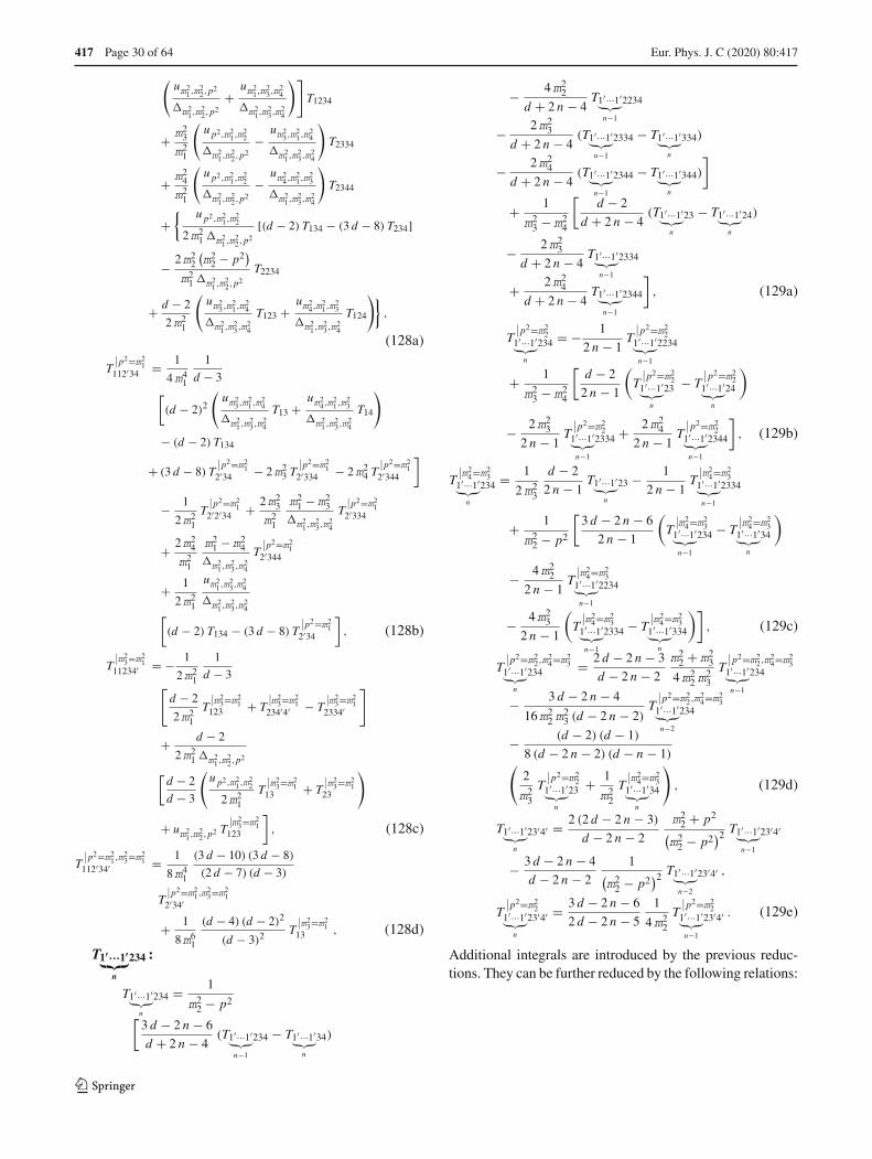
417 Page 30 of 64 Eur. Phys. J. C (2020) 80 :417
(um2
1,m22,p2
m21,m2
2,p2+
um21,m2
3,m24
m21,m2
3,m24
)]
T1234
+ m23
m21
(u p2,m2
1,m22
m21,m2
2,p2−
um23,m2
1,m24
m21,m2
3,m24
)
T2334
+ m24
m21
(u p2,m2
1,m22
m21,m2
2,p2−
um24,m2
1,m23
m21,m2
3,m24
)
T2344
+{ u p2,m2
1,m22
2m21 m2
1,m22,p2
[(d − 2) T134 − (3 d − 8) T234]
− 2m22
(m2
2 − p2)
m21 m2
1,m22,p2
T2234
+ d − 2
2m21
(um2
3,m21,m2
4
m21,m2
3,m24
T123 +um2
4,m21,m2
3
m21,m2
3,m24
T124
)},
(128a)
T∣∣p2=m2
1112′34 = 1
4m41
1
d − 3[(d − 2)2
(um2
3,m21,m2
4
m21,m2
3,m24
T13 +um2
4,m21,m2
3
m21,m2
3,m24
T14
)
− (d − 2) T134
+ (3 d − 8) T∣∣p2=m2
12′34 − 2m2
3 T∣∣p2=m2
12′334 − 2m2
4 T∣∣p2=m2
12′344
]
− 1
2m21
T∣∣p2=m2
12′2′34 + 2m2
3
m21
m21 − m2
3
m21,m2
3,m24
T∣∣p2=m2
12′334
+ 2m24
m21
m21 − m2
4
m21,m2
3,m24
T∣∣p2=m2
12′344
+ 1
2m21
um21,m2
3,m24
m21,m2
3,m24[
(d − 2) T134 − (3 d − 8) T∣∣p2=m2
12′34
], (128b)
T∣∣m2
3=m21
11234′ = − 1
2m21
1
d − 3[d − 2
2m21
T∣∣m2
3=m21
123 + T∣∣m2
3=m21
234′4′ − T∣∣m2
3=m21
2334′
]
+ d − 2
2m21 m2
1,m22,p2
[d − 2
d − 3
(u p2,m2
1,m22
2m21
T∣∣m2
3=m21
13 + T∣∣m2
3=m21
23
)
+ um21,m2
2,p2 T∣∣m2
3=m21
123
], (128c)
T∣∣p2=m2
1,m23=m2
1112′34′ = 1
8m41
(3 d − 10) (3 d − 8)
(2 d − 7) (d − 3)
T∣∣p2=m2
1,m23=m2
12′34′
+ 1
8m61
(d − 4) (d − 2)2
(d − 3)2 T∣∣m2
3=m21
13 , (128d)
T1′···1′︸︷︷︸
n
234 :
T1′···1′︸︷︷︸
n
234 = 1
m22 − p2
[3 d − 2 n − 6
d + 2 n − 4(T1′···1′
︸︷︷︸n−1
234 − T1′···1′︸︷︷︸
n
34)
− 4m22
d + 2 n − 4T1′···1′︸︷︷︸n−1
2234
− 2m23
d + 2 n − 4(T1′···1′
︸︷︷︸n−1
2334 − T1′···1′︸︷︷︸
n
334)
− 2m24
d + 2 n − 4(T1′···1′
︸︷︷︸n−1
2344 − T1′···1′︸︷︷︸
n
344)
]
+ 1
m23 − m2
4
[d − 2
d + 2 n − 4(T1′···1′
︸︷︷︸n
23 − T1′···1′︸︷︷︸
n
24)
− 2m23
d + 2 n − 4T1′···1′︸︷︷︸n−1
2334
+ 2m24
d + 2 n − 4T1′···1′︸︷︷︸n−1
2344
], (129a)
T∣∣p2=m2
21′···1′︸︷︷︸
n
234 = − 1
2 n − 1T
∣∣p2=m2
21′···1′︸︷︷︸n−1
2234
+ 1
m23 − m2
4
[d − 2
2 n − 1
(T
∣∣p2=m2
21′···1′︸︷︷︸
n
23 − T∣∣p2=m2
21′···1′︸︷︷︸
n
24
)
− 2m23
2 n − 1T
∣∣p2=m2
21′···1′︸︷︷︸n−1
2334 + 2m24
2 n − 1T
∣∣p2=m2
21′···1′︸︷︷︸n−1
2344
], (129b)
T∣∣m2
4=m23
1′···1′︸︷︷︸
n
234 = 1
2m23
d − 2
2 n − 1T1′···1′︸︷︷︸
n
23 − 1
2 n − 1T
∣∣m2
4=m23
1′···1′︸︷︷︸n−1
2334
+ 1
m22 − p2
[3 d − 2 n − 6
2 n − 1
(T
∣∣m24=m2
31′···1′︸︷︷︸n−1
234 − T∣∣m2
4=m23
1′···1′︸︷︷︸
n
34
)
− 4m22
2 n − 1T
∣∣m2
4=m23
1′···1′︸︷︷︸n−1
2234
− 4m23
2 n − 1
(T
∣∣m2
4=m23
1′···1′︸︷︷︸n−1
2334 − T∣∣m2
4=m23
1′···1′︸︷︷︸
n
334
)], (129c)
T∣∣p2=m2
2,m24=m2
31′···1′︸︷︷︸
n
234 = 2 d − 2 n − 3
d − 2 n − 2
m22 + m2
3
4m22 m
23
T∣∣p2=m2
2,m24=m2
31′···1′︸︷︷︸n−1
234
− 3 d − 2 n − 4
16m22 m
23 (d − 2 n − 2)
T∣∣p2=m2
2,m24=m2
31′···1′︸︷︷︸n−2
234
− (d − 2) (d − 1)
8 (d − 2 n − 2) (d − n − 1)(
2
m23
T∣∣p2=m2
21′···1′︸︷︷︸
n
23 + 1
m22
T∣∣m2
4=m23
1′···1′︸︷︷︸
n
34
)
, (129d)
T1′···1′︸︷︷︸
n
23′4′ = 2 (2 d − 2 n − 3)
d − 2 n − 2
m22 + p2
(m2
2 − p2)2 T1′···1′
︸︷︷︸n−1
23′4′
− 3 d − 2 n − 4
d − 2 n − 2
1(m2
2 − p2)2 T1′···1′
︸︷︷︸n−2
23′4′ ,
T∣∣p2=m2
21′···1′︸︷︷︸
n
23′4′ = 3 d − 2 n − 6
2 d − 2 n − 5
1
4m22
T∣∣p2=m2
21′···1′︸︷︷︸n−1
23′4′ . (129e)
Additional integrals are introduced by the previous reduc-tions. They can be further reduced by the following relations:
123

Eur. Phys. J. C (2020) 80 :417 Page 31 of 64 417
T1′···1′︸︷︷︸
n
2234 :
T1′···1′︸︷︷︸
n
2234 = 1
m22 − p2
[(2 d − 2 n − 5) T1′···1′
︸︷︷︸n
234 − T1′···1′︸︷︷︸n−1
2234
− 2m23 T1′···1′
︸︷︷︸n
2334 − 2m24 T1′···1′
︸︷︷︸n
2344
], (130a)
T∣∣p2=m2
21′···1′︸︷︷︸
n
2234 = 1
4m22
[(3 d − 2 n − 8)
(T
∣∣p2=m2
21′···1′︸︷︷︸
n
234 − T1′···1′︸︷︷︸n+1
34
)
− 2m23
(T
∣∣p2=m2
21′···1′︸︷︷︸
n
2334 − T1′···1′︸︷︷︸n+1
334
)
− 2m24
(T
∣∣p2=m22
1′···1′︸︷︷︸
n
2344 − T1′···1′︸︷︷︸n+1
344
)], (130b)
T1′···1′︸︷︷︸
n
2334 :
T1′···1′︸︷︷︸
n
2334 = d − 3
m23 − m2
4
T1′···1′︸︷︷︸
n
234
+ d − 2(m2
3 − m24
)2 T1′···1′︸︷︷︸
n
24 − 2m24(
m23 − m2
4
)2 T1′···1′︸︷︷︸n−1
2344
+ m23 + m2
4(m2
3 − m24
)2
(
T1′···1′︸︷︷︸n−1
2334 − d − 2
2m23
T1′···1′︸︷︷︸
n
23
)
, (131a)
T∣∣m2
4=m23
1′···1′︸︷︷︸
n
2334 = d − 2 n − 2
(2 n − 1)(m2
2 − p2)
[d − 2
4m23
T∣∣m2
4=m23
1′···1′︸︷︷︸
n
34 − 3 d − 2 n − 6
4m23
T∣∣m2
4=m23
1′···1′︸︷︷︸n−1
234
+ m22
m23
T∣∣m2
4=m23
1′···1′︸︷︷︸n−1
2234 + T∣∣m2
4=m23
1′···1′︸︷︷︸n−1
2334
]
+ 1
4m23
[d − 3
2 n − 1
(
T∣∣m2
4=m23
1′···1′︸︷︷︸n−1
2334 − d − 2
2m23
T1′···1′︸︷︷︸
n
23) + (2 d − 2 n − 5) T∣∣m2
4=m23
1′···1′︸︷︷︸
n
234
], (131b)
T∣∣p2=m2
2,m24=m2
31′···1′︸︷︷︸
n
2334 = 1
4m23[
(2 d − 2 n − 5) T∣∣p2=m2
2,m24=m2
31′···1′︸︷︷︸
n
234 − T∣∣p2=m2
2,m24=m2
31′···1′︸︷︷︸n−1
2234
],
(131c)
T1′···1′︸︷︷︸
n
334 :
T1′···1′︸︷︷︸
n
334 = d − 2 n − 1
m23 − m2
4
T1′···1′︸︷︷︸
n
34 − 1
m23 − m2
4
T1′···1′︸︷︷︸n−1
334 ,
(132a)
T∣∣m2
4=m23
1′···1′︸︷︷︸
n
334 = d − n − 2
2m23
T∣∣m2
4=m23
1′···1′︸︷︷︸
n
34 , (132b)
The integrals with multiple index 4 can be reduced afterusing the symmetry relation 3 ↔ 4. All remaining integralsbelong to the set of Eq. (114) after applying the symmetryrelations of Eqs. (107).
A.4 Vanishing external momentum
In the limit of vanishing external momentum, p → 0, manyof the reduction rules cannot be applied directly due to man-ifest poles in p2. However, if this condition is imposedonto the integrals in the first place, their reduction becomesmuch easier. Symbolically, the implementation of this limitamounts to performing the index substitutions 2 → 1and 5 → 4 (the masses are relabelled accordingly, but inorder to distinguish the possibly different masses of repeatedindices, new subscripts are introduced).
For the tensor integrals, only the first reduction inEq. (112f) requires some special care, since it contains anexplicit pole in p2. The momentum-free equation reads
Y [3]1245
(p2 = 0
)→ Y [3]
1a1b4a4b= Y [1]+[4]
1a1b4a4b(133)
which corresponds to the first term on the right-hand sideof Eq. (112f) with p → 0. For all other tensor reductions inEqs. (112) the limit p → 0 can be taken explicitly.
In addition to the types of integrals in Eqs. (119), the fol-lowing scalar integrals appear after taking into account thesymmetry relations of Eq. (107) and partial-fraction decom-position via Eq. (121):
T1113 , T1133 , T11134 , T11334 . (134)
Further integrals with multiple massless propagators withindex 1′ can be solved with the recurrence relations givenabove. In general, the solutions for the integrals of Eq. (134)with repeated index i can be derived by computing the deriva-tive with respect to the mass mi of the scalar integral withfewer repetitions of i . The results that are not contained inEqs. (125)–(132) readT1···1︸︷︷︸
n1
3···3︸︷︷︸
n3
and T1′···1′︸︷︷︸
n1
3···3︸︷︷︸
n3
:
T 1···1︸︷︷︸n1
3···3︸︷︷︸n3
= �(n1 − d
2
)
(−m21
)n1−1�(n1) �
(1 − d
2
)�
(n3 − d
2
)
(−m23
)n3−1�(n3) �
(1 − d
2
) T13 ,
(135a)
T1′···1′︸︷︷︸n1
3···3︸︷︷︸n3
= 0 , (135b)
T1···1︸︷︷︸
n1
3···3︸︷︷︸
n3
4 and T1′···1′︸︷︷︸
n1
3···3︸︷︷︸
n3
4 :
0 = (n3 − 1) um24,m
21,m
23T 1···1︸︷︷︸
n1
3···3︸︷︷︸n3
4
− (n3 − 1) T 1···1︸︷︷︸n1−1
3···3︸︷︷︸n3
4 + (n3 − 1) T 1···1︸︷︷︸n1
3···3︸︷︷︸n3
123
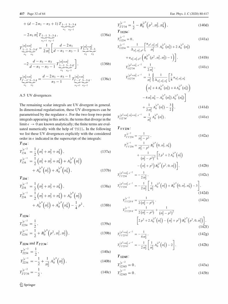
417 Page 32 of 64 Eur. Phys. J. C (2020) 80 :417
+ (d − 2 n1 − n3 + 1) T 1···1︸︷︷︸n1
3···3︸︷︷︸n3−1
4
− 2 n1 m21 T 1···1︸︷︷︸
n1+1
3···3︸︷︷︸n3−1
4 , (136a)
T∣∣m2
3=m21
1···1︸︷︷︸n1
3···3︸︷︷︸n3
4′ = 1
2m21
[d − 2 n1
d − n1 − n3 − 1T
∣∣m2
3=m21
1···1︸︷︷︸n1
3···3︸︷︷︸n3
−2d − n1 − n3
d − n1 − n3 − 1T
∣∣m2
3=m21
1···1︸︷︷︸n1
3···3︸︷︷︸n3−1
4′
], (136b)
T∣∣m2
4=m23
1′···1′︸︷︷︸n1
3···3︸︷︷︸n3
4 = d − 2 n1 − n3 − 1
n3 − 1T
∣∣m2
4=m23
1′···1′︸︷︷︸n1+1
3···3︸︷︷︸n3−1
4 . (136c)
A.5 UV divergences
The remaining scalar integrals are UV divergent in general.In dimensional regularisation, these UV divergences can beparametrised by the regulator ε. For the two-loop two-pointintegrals appearing in this article, the terms that diverge in thelimit ε → 0 are known analytically; the finite terms are eval-uated numerically with the help of TSIL. In the followingwe list these UV divergences explicitly with the consideredorder in ε indicated in the superscript of the integrals:T134 :
T∣∣ε−2
134 = 1
2
(m2
1 + m23 + m2
4
), (137a)
T∣∣ε−1
134 = 1
2
(m2
1 + m23 + m2
4
)+ A
∣∣ε0
0
(m2
1
)
+ A∣∣ε0
0
(m2
3
)+ A
∣∣ε0
0
(m2
4
), (137b)
T234 :
T∣∣ε−2
234 = 1
2
(m2
2 + m23 + m2
4
), (138a)
T∣∣ε−1
234 = 1
2
(m2
2 + m23 + m2
4
)+ A
∣∣ε0
0
(m2
2
)
+ A∣∣ε0
0
(m2
3
)+ A
∣∣ε0
0
(m2
4
)− 1
4p2 , (138b)
T1234 :
T∣∣ε−2
1234 = 1
2, (139a)
T∣∣ε−1
1234 = 1
2+ B
∣∣ε0
0
(p2,m2
1,m22
), (139b)
T2234 and T2′2′34 :
T∣∣ε−2
2234 = 1
2, (140a)
T∣∣ε−1
2234 = −1
2+ 1
m22
A∣∣ε0
0
(m2
2
), (140b)
T∣∣ε−2
2′2′34 = −1
2, (140c)
T∣∣ε−1
2′2′34 = 1
2− B
∣∣ε0
0
(p2,m2
3,m24
), (140d)
T11234 :
T∣∣ε−2
11234 = 0 , (141a)
T∣∣ε−1
11234 = 1
m21,m2
2,p2
[u p2,m21,m2
2
m21
A∣∣ε0
0
(m2
1
) + 2 A∣∣ε0
0
(m2
2
)
+ um21,m2
2,p2
(B
∣∣ε0
0
(p2,m2
1,m22
) − 1
)], (141b)
T∣∣p2=m2
1, ε−2
112′34 = 1
2m21
, (141c)
T∣∣p2=m2
1, ε−1
112′34 = 1
m21
{1
m21,m2
3,m24
[3
8um2
1,m23,m2
4
(m2
1 + 4 A∣∣ε0
0
(m2
3
) + 4 A∣∣ε0
0
(m2
4
))
− 4m23 m
24 − A
∣∣ε0
0
(m2
3
)A
∣∣ε0
0
(m2
4
)]
+ 1
2m21
A∣∣ε0
0
(m2
1
) − 3
2
}, (141d)
T∣∣p2=m2
1,m23=m2
1, ε−1
112′34′ = 1
m41
A∣∣ε0
0
(m2
1
), (141e)
T1′1′234 :
T∣∣ε−2
1′1′234 = 1
m22 − p2
, (142a)
T∣∣ε−1
1′1′234 = 1
m22 − p2
B∣∣ε0
0
(0,m2
3,m24
)
+ 1(m2
2 − p2)2
[2 p2 + 2 A
∣∣ε0
0
(m2
2
)
−(m2
2 + p2)B
∣∣ε0
0
(p2, 0,m2
2
)], (142b)
T∣∣p2=m2
2, ε−2
1′1′234 = − 1
2m22
, (142c)
T∣∣p2=m2
2, ε−1
1′1′234 = − 1
2m22
[1
m22
A∣∣ε0
0
(m2
2
)+ B
∣∣ε0
0
(0,m2
3,m24
)− 3
]
,
(142d)
T∣∣ε−2
1′1′23′4′ = 1
2(m2
2 − p2) , (142e)
T∣∣ε−1
1′1′23′4′ = 1
2(m2
2 − p2) + 1
(m2
2 − p2)2
[2 p2 + 2 A
∣∣ε0
0
(m2
2
)−
(m2
2 + p2)B
∣∣ε0
0
(p2, 0,m2
2
)],
(142f)
T∣∣p2=m2
2, ε−2
1′1′23′4′ = − 1
4m22
, (142g)
T∣∣p2=m2
2, ε−1
1′1′23′4′ = − 1
2m22
[1
m22
A∣∣ε0
0
(m2
2
)− 2
]
, (142h)
T12345 :
T∣∣ε−2
12345 = 0 , (143a)
T∣∣ε−1
12345 = 0 . (143b)
123

Eur. Phys. J. C (2020) 80 :417 Page 33 of 64 417
B List of renormalised Feynman diagrams
The complete list of renormalised two-loop diagrams (with polynomial remainder in the UV regulator 1/ε) for tadpoles andself-energies in ’t Hooft–Feynman gauge is shown in the following. Contributions that only exist in the MS scheme are markedby δMS. At first, we repeat the previously known results of Refs. [121,122] in our nomenclature, and then we list all newresults.
B.1 Tadpole diagrams
B.1.1 Known results
I(1)01
S(i1)
S(i2)
S(i3)
S(i4)
SSS[i1, i2, i3, 1]SSSS[i2, i3, i4, i4, 1]×1
4
{1
ε
[A0
(m2
i4
)+ m2
i4 B0
(0,m2
i2,m2i3
)]− T113
(m2
i2,m2i3,m
2i4
)}
I(1)07
S(i1)
S(i2)
S(i3)S(i4)
S(i5)
SSS[i1, i2, i5, 1]SSS[i2, i3, i4, 1]SSS[i3, i4, i5, 1]×1
4
{1
εB0
(0,m2
i2,m2i5
)− T1134
(m2
i2,m2i5,m
2i3,m
2i4
)}
I(1)24
S(i1)
S(i2)
S(i3)
S(i4)
SSS[i2, i3, i4, 1]SSSS[i1, i2, i3, i4, 1]×1
6
{1
ε
[A0
(m2
i2
)+ A0
(m2
i3
)+ A0
(m2
i4
)]− T134
(m2
i2,m2i3,m
2i4
)}
I(1)05
S(i1)
F(i2)
F(i3)S(i4)
F(i5)
mi2 mi3 mi5 e[FFS[i2, i3, i4, 1]FFS[i2, i5, i1, 1]FFS[i3, i5, i4, 1]] ×2
{− 1
εB0
(0,m2
i2,m2i5
)+ T1134
(m2
i2,m2i5,m
2i3,m
2i4
)}
+mi3 e[FFS[i2, i3, i4, 1]FFS[i2, i5, i1, 2]FFS[i3, i5, i4, 1]] ×2
{− 1
ε
[A0
(m2
i3
)+ A0
(m2
i4
)+ 0Y [1]
11
(m2
i2,m2i5
)]
+ Y [1]1134
(m2
i2,m2i5,m
2i3,m
2i4
)}
+[mi2 + mi5
]e[FFS[i2, i3, i4, 1]FFS[i2, i5, i1, 1]FFS[i3, i5, i4, 2]] ×
{− 1
ε
[2 A0
(m2
i4
)+ 0Y [1]
11
(m2
i2,m2i5
)]+ Y [1]+[3]−[4]
1134
(m2
i2,m2i5,m
2i3,m
2i4
)}
I(1)06
S(i1)
S(i2)
F(i3)F(i4)
S(i5)
mi3 mi4 e[FFS[i3, i4, i2, 1]FFS[i3, i4, i5, 1]]SSS[i1, i2, i5, 1]×{− 1
εB0
(0,m2
i2,m2i5
)+ T1134
(m2
i2,m2i5,m
2i3,m
2i4
)}
+ e[FFS[i3, i4, i2, 1]FFS[i3, i4, i5, 2]]SSS[i1, i2, i5, 1]×1
2
{1
ε
[0Y [1]
11
(m2
i2,m2i5
)− 2
(m2
i3 + m2i4
)B0
(0,m2
i2,m2i5
)]
− Y [1]−[3]−[4]1134
(m2
i2,m2i5,m
2i3,m
2i4
)}
123

417 Page 34 of 64 Eur. Phys. J. C (2020) 80 :417
B.1.2 New results with vectors
I(1)02
S(i1)
S(i2)
S(i3)
V(i4)
SSS[i1, i2, i3, 1]SSVV[i2, i3, i4, i4, 1]×1
2
{− 1
ε
[2m2
i4 B0
(0,m2
i2,m2i3
)+ (2 − δMS ε) A0
(m2
i4
)]
+ (2 − δMS ε) T113
(m2
i2,m2i3,m
2i4
)}
I(1)03
S(i1)
V(i2)
V(i3)
S(i4)
SSVV[i4, i4, i2, i3, 1]SVV[i1, i2, i3, 1]×1
2
{1
ε
[2 A0
(m2
i4
)+ (2 − δMS ε)m2
i4 B0
(0,m2
i2,m2i3
)]
− (2 − δMS ε) T113
(m2
i2,m2i3,m
2i4
)}
I(1)04
S(i1)
V(i2)
V(i3)
V(i4)
SVV[i1, i2, i3, 1]×[4VVVV[i2, i3, i4, i4, 1] + VVVV[i2, i3, i4, i4, 2] + VVVV[i2, i3, i4, i4, 3]
]×
1
2
{− 1
ε(2 − δMS ε)
[A0
(m2
i4
)+ m2
i4 B0
(0,m2
i2,m2i3
)]}
SVV[i1, i2, i3, 1]×[(4 − 2 δMS ε)VVVV[i2, i3, i4, i4, 1] + VVVV[i2, i3, i4, i4, 2] + VVVV[i2, i3, i4, i4, 3]
]×
1
2
{(2 − δMS ε) T113
(m2
i2,m2i3,m
2i4
)}
I(1)12
S(i1)
S(i2)
S(i3)S(i4)
V(i5)
SSS[i2, i3, i4, 1]SSV[i1, i2, i5, 1]SSV[i3, i4, i5, 1]×1
2
{1
ε
[A0
(m2
i3
)− A0
(m2
i4
)]− Y [3]−[4]
1134
(m2
i2,m2i5,m
2i3,m
2i4
)}
I(1)13
S(i1)
S(i2)
S(i3)V(i4)
S(i5) SSS[i1, i2, i5, 1]SSV[i2, i3, i4, 1]SSV[i3, i5, i4, 1]×1
2
{− 1
ε
[A0
(m2
i3
)+ 2 (2 − δMS ε) A0
(m2
i4
)
+(m2
i3 + m2i4
)B0
(0,m2
i2,m2i5
)+ 2 0Y [1]
11
(m2
i2,m2i5
)]
+ Y 2[1]−[3]+2[4]1134
(m2
i2,m2i5,m
2i3,m
2i4
)}
I(1)17
S(i1)
V(i2)
S(i3)S(i4)
V(i5) SSV[i3, i4, i2, 1]SSV[i3, i4, i5, 1]SVV[i1, i2, i5, 1]×1
4
{1
ε
[− A0
(m2
i3
)− A0
(m2
i4
)+ 1
3 (3 − 2 δMS ε) 0Y [1]11
(m2
i2,m2i5
)
− 2 (2 − δMS ε)(m2
i3 + m2i4
)B0
(0,m2
i2,m2i5
)]
− Y [1]−2[3]−2[4]1134
(m2
i2,m2i5,m
2i3,m
2i4
)}
I(1)18
S(i1)
S(i2)
S(i3)V(i4)
V(i5)SSV[i1, i2, i5, 1]SSV[i2, i3, i4, 1]SVV[i3, i4, i5, 1]×1
2
{1
ε
[2 A0
(m2
i3
)+ 3 0Y [1]
11
(m2
i2,m2i5
)+ 2 (2 − δMS ε) A0
(m2
i4
)]
− Y 3[1]−[3]+[4]1134
(m2
i2,m2i5,m
2i3,m
2i4
)}
123

Eur. Phys. J. C (2020) 80 :417 Page 35 of 64 417
I(1)19
S(i1)
S(i2)
V(i3)V(i4)
S(i5)
SSS[i1, i2, i5, 1]SVV[i2, i3, i4, 1]SVV[i5, i3, i4, 1]×1
2
{2
εB0
(0,m2
i2,m2i5
)− (2 − δMS ε) T1134
(m2
i2,m2i5,m
2i3,m
2i4
)}
I(1)21
S(i1)
V(i2)
S(i3)V(i4)
V(i5)
SVV[i1, i2, i5, 1]SVV[i3, i2, i4, 1]SVV[i3, i4, i5, 1]×{− 1
ε(2 − δMS ε) B0
(0,m2
i2,m2i5
)+ (2 − δMS ε) T1134
(m2
i2,m2i5,m
2i3,m
2i4
)}
I(1)22
S(i1)
S(i2)
V(i3)V(i4)
V(i5)SSV[i1, i2, i5, 1]SVV[i2, i3, i4, 1]VVV[i3, i4, i5, 1]×1
4
{− 3
ε(2 − δMS ε)
[A0
(m2
i3
)− A0
(m2
i4
)]
+ 2 (3 − 2 δMS ε) Y [3]−[4]1134
(m2
i2,m2i5,m
2i3,m
2i4
)}
I(1)23
S(i1)
V(i2)
V(i3)V(i4)
V(i5)SVV[i1, i2, i5, 1]VVV[i2, i3, i4, 1]VVV[i3, i4, i5, 1]×1
4
{− 1
ε(2 − δMS ε)
[9 A0
(m2
i3
)+ 9 A0
(m2
i4
)
+ 9(m2
i3 + m2i4
)B0
(0,m2
i2,m2i5
)− 0Y [1]
11
(m2
i2,m2i5
)]
− 11
3 ε(3 − 2 δMS ε) 0Y [1]
11
(m2
i2,m2i5
)
+ 3 (3 − 2 δMS ε) Y [1]+[3]+[4]1134
(m2
i2,m2i5,m
2i3,m
2i4
)}
I(1)25
S(i1)
S(i2)
V(i3)
V(i4)
SSVV[i1, i2, i3, i4, 1]SVV[i2, i3, i4, 1]×{
1
ε
[2 A0
(m2
i2
)+ (2 − δMS ε)
[A0
(m2
i3
)+ A0
(m2
i4
)]]
− (2 − δMS ε) T134
(m2
i2,m2i3,m
2i4
)}
123

417 Page 36 of 64 Eur. Phys. J. C (2020) 80 :417
B.1.3 New results with fermions and vectors
I(1)10
S(i1)
F(i2)
F(i3)V(i4)
F(i5)
mi2 mi3 mi5 e[FFS[i2, i5, i1, 1]FFV[i2, i3, i4, 2]FFV[i3, i5, i4, 1]] ×4
{2
εB0
(0,m2
i2,m2i5
)− (2 − δMS ε) T1134
(m2
i2,m2i5,m
2i3,m
2i4
)}
+mi3 e[FFS[i2, i5, i1, 1]FFV[i2, i3, i4, 1]FFV[i3, i5, i4, 2]] ×4
{1
ε
[2 A0
(m2
i3
)+ 2 0Y [1]
11
(m2
i2,m2i5
)+ (2 − δMS ε) A0
(m2
i4
)]
− (2 − δMS ε) Y [1]1134
(m2
i2,m2i5,m
2i3,m
2i4
)}
+[mi2 e[FFS[i2, i5, i1, 1]FFV[i2, i3, i4, 2]FFV[i3, i5, i4, 2]]+mi5 e[FFS[i2, i5, i1, 1]FFV[i2, i3, i4, 1]FFV[i3, i5, i4, 1]]
]×
2
{− 1
ε
[0Y [1]
11
(m2
i2,m2i5
)+ (2 − δMS ε) A0
(m2
i4
)]
+ (1 − δMS ε) Y [1]+[3]−[4]1134
(m2
i2,m2i5,m
2i3,m
2i4
)}
I(1)16
S(i1)
V(i2)
F(i3)F(i4)
V(i5)
mi3 mi4 e[FFV[i3, i4, i2, 1]FFV[i3, i4, i5, 1]]SVV[i1, i2, i5, 1]×2
{1
ε(2 − δMS ε) B0
(0,m2
i2,m2i5
)− (2 − δMS ε) T1134
(m2
i2,m2i5,m
2i3,m
2i4
)}
+ e[FFV[i3, i4, i2, 1]FFV[i3, i4, i5, 2]]SVV[i1, i2, i5, 1]×{
1
ε
[− (2 − δMS ε)
(m2
i3 + m2i4
)B0
(0,m2
i2,m2i5
)
+ 13 (3 − 2 δMS ε) 0Y [1]
11
(m2
i2,m2i5
)]
− (1 − δMS ε) Y [1]−[3]−[4]1134
(m2
i2,m2i5,m
2i3,m
2i4
)}
I(1)11
S(i1)
S(i2)
F(i3)F(i4)
V(i5)
mi3 e[FFS[i3, i4, i2, 1]FFV[i3, i4, i5, 2]]SSV[i1, i2, i5, 1]×{
1
ε
[2 A0
(m2
i3
)+ 0Y [1]
11
(m2
i2,m2i5
)]− Y [1]−[3]+[4]
1134
(m2
i2,m2i5,m
2i3,m
2i4
)}
+ [i3 ↔ i4]
B.1.4 New results with ghosts
I(1)08
S(i1)
S(i2)
U(i3)U(i4)
S(i5)
SSS[i1, i2, i5, 1]SUU[i2,−i3, i4, 1]SUU[i5,−i4, i3, 1]×1
4
{− 1
εB0
(0,m2
i2,m2i5
)+ T1134
(m2
i2,m2i5,m
2i3,m
2i4
)}
I(1)09
S(i1)
U(i2)
S(i3)U(i4)
U(i5)
SUU[i1,−i5, i2, 1]SUU[i3,−i2, i4, 1]SUU[i3,−i4, i5, 1]×1
2
{− 1
εB0
(0,m2
i2,m2i5
)+ T1134
(m2
i2,m2i5,m
2i3,m
2i4
)}
123

Eur. Phys. J. C (2020) 80 :417 Page 37 of 64 417
I(1)14
S(i1)
S(i2)
U(i3)U(i4)
V(i5)
SSV[i1, i2, i5, 1]SUU[i2,−i3, i4, 1]UUV[−i4, i3, i5, 1]×1
2
{1
ε
[2 A0
(m2
i3
)+ 0Y [1]
11
(m2
i2,m2i5
)]− Y [1]−[3]+[4]
1134
(m2
i2,m2i5,m
2i3,m
2i4
)}
I(1)15
S(i1)
U(i2)
U(i3)V(i4)
U(i5)
[SUU[i1,−i5, i2, 1]UUV[−i2, i3, i4, 1]UUV[−i3, i5, i4, 1]+SUU[i1, i5,−i2, 1]UUV[i2,−i3, i4, 2]UUV[i3,−i5, i4, 2]
]
1
4
{1
ε
[0Y [1]
11
(m2
i2,m2i5
)+ (2 − δMS ε) A0
(m2
i4
)]
− Y [1]+[3]−[4]1134
(m2
i2,m2i5,m
2i3,m
2i4
)}
I(1)20
S(i1)
V(i2)
U(i3)U(i4)
V(i5)[SVV[i1, i2, i5, 1]UUV[−i3, i4, i2, 1]UUV[−i4, i3, i5, 1]+SVV[i1, i2, i5, 1]UUV[i3,−i4, i2, 2]UUV[i4,−i3, i5, 2]
]×
1
8
{1
ε
[13 (3 − δMS ε) 0Y [1]
11
(m2
i2,m2i5
)− (2 − δMS ε)
(m2
i3 + m2i4
)B0
(0,m2
i2,m2i5
)]
− Y [1]−[3]−[4]1134
(m2
i2,m2i5,m
2i3,m
2i4
)}
B.2 Self-energy diagrams
B.2.1 Known results with only scalars
I(2)001
S(i1) S(i2)
S(i3)
S(i4) S(i5)
S(i6)
SSS[i1, i3, i4, 1]SSS[i2, i3, i5, 1]SSSS[i4, i5, i6, i6, 1]×1
2
{1
εm2
i60T112
(m2
i4,m2i5,m
2i3
)− T1123
(m2
i4,m2i5,m
2i3,m
2i6
)}
I(2)009
S(i1) S(i2)
S(i3)
S(i4)
S(i5)
S(i6)
SSS[i1, i3, i6, 1]SSS[i3, i4, i5, 1]SSSS[i2, i4, i5, i6, 1]×1
2
{1
εB0
(p2,m2
i3,m2i6
)− T1234
(m2
i3,m2i6,m
2i4,m
2i5
)}
I(2)015
S(i1) S(i2)
S(i3)
S(i4)
S(i5)
S(i6)
I(2)009
∣∣∣i1↔i2
123

417 Page 38 of 64 Eur. Phys. J. C (2020) 80 :417
I(2)024
S(i1) S(i2)
S(i3) S(i4)
S(i5)
S(i6) S(i7)
SSS[i1, i3, i6, 1]SSS[i2, i4, i7, 1]SSS[i3, i4, i5, 1]SSS[i5, i6, i7, 1]×1
2
{− T12345
(m2
i3,m2i6,m
2i5,m
2i4,m
2i7
)}
I(2)059
S(i1) S(i2)
S(i3)
S(i4)
S(i5)
S(i6)
S(i7)SSS[i1, i3, i4, 1]SSS[i2, i3, i7, 1]SSS[i4, i5, i6, 1]SSS[i5, i6, i7, 1]×1
2
{1
ε
0T112
(m2
i4,m2i7,m
2i3
)− T11234
(m2
i4,m2i7,m
2i3,m
2i5,m
2i6
)}
I(2)101
S(i1) S(i2)
S(i3) S(i4)
S(i5)
SSSS[i1, i2, i3, i4, 1]SSSS[i3, i4, i5, i5, 1]×1
4
{1
ε
[A0
(m2
i5
)+ m2
i5 B0
(0,m2
i3,m2i4
)]− T113
(m2
i3,m2i4,m
2i5
)}
I(2)105
S(i1) S(i2)
S(i3)
S(i4)
S(i5)
S(i6) SSS[i1, i3, i4, 1]SSS[i2, i5, i6, 1]SSSS[i3, i4, i5, i6, 1]×1
4
{1
ε
[B0
(p2,m2
i3,m2i4
)+ B0
(p2,m2
i5,m2i6
)]
− T1245
(m2
i3,m2i4,m
2i5,m
2i6
)}
I(2)111
S(i1) S(i2)
S(i3)
S(i4)
S(i5) S(i6)
SSS[i3, i4, i5, 1]SSS[i3, i4, i6, 1]SSSS[i1, i2, i5, i6, 1]×1
4
{1
εB0
(0,m2
i5,m2i6
)− T1134
(m2
i5,m2i6,m
2i3,m
2i4
)}
I(2)120
S(i1) S(i2)
S(i3)
S(i4)
S(i5)
SSSS[i1, i3, i4, i5, 1]SSSS[i2, i3, i4, i5, 1]×1
6
{1
ε
[A0
(m2
i3
)+ A0
(m2
i4
)+ A0
(m2
i5
)]− T234
(m2
i3,m2i4,m
2i5
)}
123

Eur. Phys. J. C (2020) 80 :417 Page 39 of 64 417
B.2.2 Known results with scalars and fermions
I(2)021
S(i1) S(i2)
F(i3) F(i4)
S(i5)
F(i6) F(i7)
mi3 mi4 mi6 mi7 e[FFS[i3, i4, i5, 1]FFS[i3, i6, i1, 1]FFS[i4, i7, i2, 1]FFS[i6, i7, i5, 1]] ×1
2
{T12345
(m2
i7,m2i4,m
2i5,m
2i6,m
2i3
)}
+mi3 mi4 e[FFS[i3, i4, i5, 1]FFS[i3, i6, i1, 1]FFS[i4, i7, i2, 1]FFS[i6, i7, i5, 2]] ×1
2
{Y [2]−[3]+[5]
12345
(m2
i3,m2i6,m
2i5,m
2i4,m
2i7
)}
+mi3 mi7 e[FFS[i3, i4, i5, 1]FFS[i3, i6, i1, 1]FFS[i4, i7, i2, 2]FFS[i6, i7, i5, 2]] ×1
2
{Y [1]−[3]+[5]−[6]
12345
(m2
i3,m2i6,m
2i5,m
2i4,m
2i7
)}
+mi3 mi6 e[FFS[i3, i4, i5, 1]FFS[i3, i6, i1, 1]FFS[i4, i7, i2, 2]FFS[i6, i7, i5, 1]] ×1
2
{− 2
εB0
(p2,m2
i3,m2i6
)+ Y [4]+[5]−[6]
12345
(m2
i3,m2i6,m
2i5,m
2i4,m
2i7
)}
+e[FFS[i3, i4, i5, 1]FFS[i3, i6, i1, 2]FFS[i4, i7, i2, 2]FFS[i6, i7, i5, 1]] ×1
4
{− 2
ε
[A0
(m2
i5
)+ 0Y [1]+[2]−[6]
12
(m2
i3,m2i6
)]
+ Y 2[15]−[36]12345
(m2
i3,m2i6,m
2i5,m
2i4,m
2i7
)}
+ [(i3, i4) ↔ (i6, i7)] + [(i1, i3, i6) ↔ (i2, i4, i7)] + [(i1, i3, i4) ↔ (i2, i7, i6)]
I(2)022
S(i1) S(i2)
F(i3) S(i4)
F(i5)
F(i6) S(i7)
mi3 mi5 mi6 e[FFS[i3, i5, i4, 1]FFS[i3, i6, i1, 1]FFS[i5, i6, i7, 1]]SSS[i2, i4, i7, 1]×{T12345
(m2
i7,m2i4,m
2i5,m
2i6,m
2i3
)}
+mi3 e[FFS[i3, i5, i4, 1]FFS[i3, i6, i1, 1]FFS[i5, i6, i7, 2]]SSS[i2, i4, i7, 1]×{− 2
εB0
(p2,m2
i4,m2i7
)+ Y [2]+[3]−[5]
12345
(m2
i3,m2i6,m
2i5,m
2i4,m
2i7
)}
+mi5 e[FFS[i3, i5, i4, 1]FFS[i3, i6, i1, 2]FFS[i5, i6, i7, 1]]SSS[i2, i4, i7, 1]×1
2
{− 2
εB0
(p2,m2
i4,m2i7
)+ Y 2[1]−[6]
12345
(m2
i3,m2i6,m
2i5,m
2i4,m
2i7
)}
+ [(i3, i4) ↔ (i6, i7)]
I(2)023
S(i1) S(i2)
S(i3) F(i4)
F(i5)
S(i6) F(i7)
I(2)022
∣∣∣i1↔i2, i3↔i4, i6↔i7
123

417 Page 40 of 64 Eur. Phys. J. C (2020) 80 :417
I(2)057
S(i1) S(i2)
F(i3)
F(i4)
F(i5)
S(i6)
F(i7)
mi3 mi4 mi5 mi7 e[FFS[i3, i4, i1, 1]FFS[i3, i7, i2, 1]FFS[i4, i5, i6, 1]FFS[i5, i7, i6, 1]] ×2
{− 1
ε
0T112
(m2
i4,m2i7,m
2i3
)+ T11234
(m2
i4,m2i7,m
2i3,m
2i5,m
2i6
)}
+mi3 mi5 e[FFS[i3, i4, i1, 1]FFS[i3, i7, i2, 1]FFS[i4, i5, i6, 2]FFS[i5, i7, i6, 2]] ×2
{− 1
ε
0Y [1]112
(m2
i4,m2i7,m
2i3
)+ Y [1]
11234
(m2
i4,m2i7,m
2i3,m
2i5,m
2i6
)}
+mi4 mi7 e[FFS[i3, i4, i1, 1]FFS[i3, i7, i2, 2]FFS[i4, i5, i6, 1]FFS[i5, i7, i6, 2]] ×1
2
{− 1
ε
0Y [1]+[2]−[6]112
(m2
i4,m2i7,m
2i3
)+ 2 Y [2]+[3]−[5]
11234
(m2
i4,m2i7,m
2i3,m
2i5,m
2i6
)}
+mi3 mi4 e[FFS[i3, i4, i1, 1]FFS[i3, i7, i2, 1]FFS[i4, i5, i6, 1]FFS[i5, i7, i6, 2]] ×2
{− 1
ε
0Y [1]112
(m2
i4,m2i7,m
2i3
)+ Y [1]+[3]−[4]
11234
(m2
i4,m2i7,m
2i3,m
2i5,m
2i6
)}
+mi4 mi5 e[FFS[i3, i4, i1, 1]FFS[i3, i7, i2, 2]FFS[i4, i5, i6, 1]FFS[i5, i7, i6, 1]] ×2
{− 1
ε
0Y [1]+[2]−[6]112
(m2
i4,m2i7,m
2i3
)+ Y [1]+[2]−[6]
11234
(m2
i4,m2i7,m
2i3,m
2i5,m
2i6
)}
+e[FFS[i3, i4, i1, 1]FFS[i3, i7, i2, 2]FFS[i4, i5, i6, 2]FFS[i5, i7, i6, 1]] ×1
2
{− 1
ε
[4 A0
(m2
i6
)+ 0Y [11]+[12]−[16]
112
(m2
i4,m2i7,m
2i3
)]
+ 2 Y [12]+[14]−[15]−[23]+[36]+[24]−[46]11234
(m2
i4,m2i7,m
2i3,m
2i6,m
2i5
)}
+ [(i1, i4) ↔ (i2, i7)]
I(2)058
S(i1) S(i2)
S(i3)
S(i4)
F(i5)
F(i6)
S(i7)
mi5 mi6 e[FFS[i5, i6, i4, 1]FFS[i5, i6, i7, 1]]SSS[i1, i3, i4, 1]SSS[i2, i3, i7, 1]×2
{− 1
ε
0T112
(m2
i4,m2i7,m
2i3
)+ T11234
(m2
i4,m2i7,m
2i3,m
2i5,m
2i6
)}
+e[FFS[i5, i6, i4, 1]FFS[i5, i6, i7, 2]]SSS[i1, i3, i4, 1]SSS[i2, i3, i7, 1]×{
1
ε
[− 2
(m2
i5 + m2i6
)0T112
(m2
i4,m2i7,m
2i3
)+ 0Y [1]
112
(m2
i4,m2i7,m
2i3
)]
− Y [1]−[3]−[4]11234
(m2
i4,m2i7,m
2i3,m
2i5,m
2i6
)}
I(2)110
S(i1) S(i2)
F(i3)
F(i4)
S(i5) S(i6)
mi3 mi4 e[FFS[i3, i4, i5, 1]FFS[i3, i4, i6, 1]]SSSS[i1, i2, i5, i6, 1]×{− 1
εB0
(0,m2
i5,m2i6
)+ T1134
(m2
i5,m2i6,m
2i3,m
2i4
)}
+e[FFS[i3, i4, i5, 1]FFS[i3, i4, i6, 2]]SSSS[i1, i2, i5, i6, 1]×1
2
{1
ε
[− 2
(m2
i3 + m2i4
)B0
(0,m2
i5,m2i6
)+ 0Y [1]
11
(m2
i5,m2i6
)]
− Y [1]−[3]−[4]1134
(m2
i5,m2i6,m
2i3,m
2i4
)}
B.2.3 Known results with scalars and one vector
I(2)002
S(i1) S(i2)
S(i3)
S(i4) S(i5)
V(i6)
SSS[i1, i3, i4, 1]SSS[i2, i3, i5, 1]SSVV[i4, i5, i6, i6, 1]×{− 2
εm2
i60T112
(m2
i4,m2i5,m
2i3
)+ (2 − δMS ε) T1123
(m2
i4,m2i5,m
2i3,m
2i6
)}
123
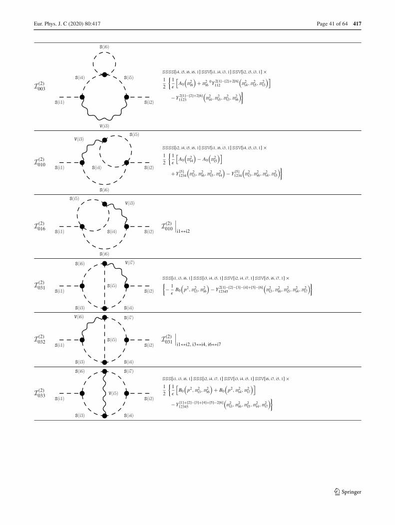
Eur. Phys. J. C (2020) 80 :417 Page 41 of 64 417
I(2)003
S(i1) S(i2)
V(i3)
S(i4) S(i5)
S(i6)
SSSS[i4, i5, i6, i6, 1]SSV[i1, i4, i3, 1]SSV[i2, i5, i3, 1]×1
2
{1
ε
[A0
(m2
i6
)+ m2
i60Y 2[1]−[2]+2[6]
112
(m2
i4,m2i5,m
2i3
)]
− Y 2[1]−[2]+2[6]1123
(m2
i4,m2i5,m
2i3,m
2i6
)}
I(2)010
S(i1) S(i2)
V(i3)
S(i4)
S(i5)
S(i6)
SSSS[i2, i4, i5, i6, 1]SSV[i1, i6, i3, 1]SSV[i4, i5, i3, 1]×1
2
{1
ε
[A0
(m2
i4
)− A0
(m2
i5
)]
+ Y [5]1234
(m2
i3,m2i6,m
2i5,m
2i4
)− Y [5]
1234
(m2
i3,m2i6,m
2i4,m
2i5
)}
I(2)016
S(i1) S(i2)
V(i3)
S(i4)
S(i5)
S(i6)
I(2)010
∣∣∣i1↔i2
I(2)031
S(i1) S(i2)
S(i3) S(i4)
S(i5)
S(i6) V(i7)
SSS[i1, i3, i6, 1]SSS[i3, i4, i5, 1]SSV[i2, i4, i7, 1]SSV[i5, i6, i7, 1]×{− 1
εB0
(p2,m2
i3,m2i6
)− Y 2[1]−[2]−[3]−[4]+[5]−[6]
12345
(m2
i3,m2i6,m
2i5,m
2i4,m
2i7
)}
I(2)032
S(i1) S(i2)
S(i3) S(i4)
S(i5)
V(i6) S(i7)
I(2)031
∣∣∣i1↔i2, i3↔i4, i6↔i7
I(2)033
S(i1) S(i2)
S(i3) S(i4)
V(i5)
S(i6) S(i7)
SSS[i1, i3, i6, 1]SSS[i2, i4, i7, 1]SSV[i3, i4, i5, 1]SSV[i6, i7, i5, 1]×1
2
{1
ε
[B0
(p2,m2
i3,m2i6
)+ B0
(p2,m2
i4,m2i7
)]
− Y [1]+[2]−[3]+[4]+[5]−2[6]12345
(m2
i3,m2i6,m
2i5,m
2i4,m
2i7
)}
123
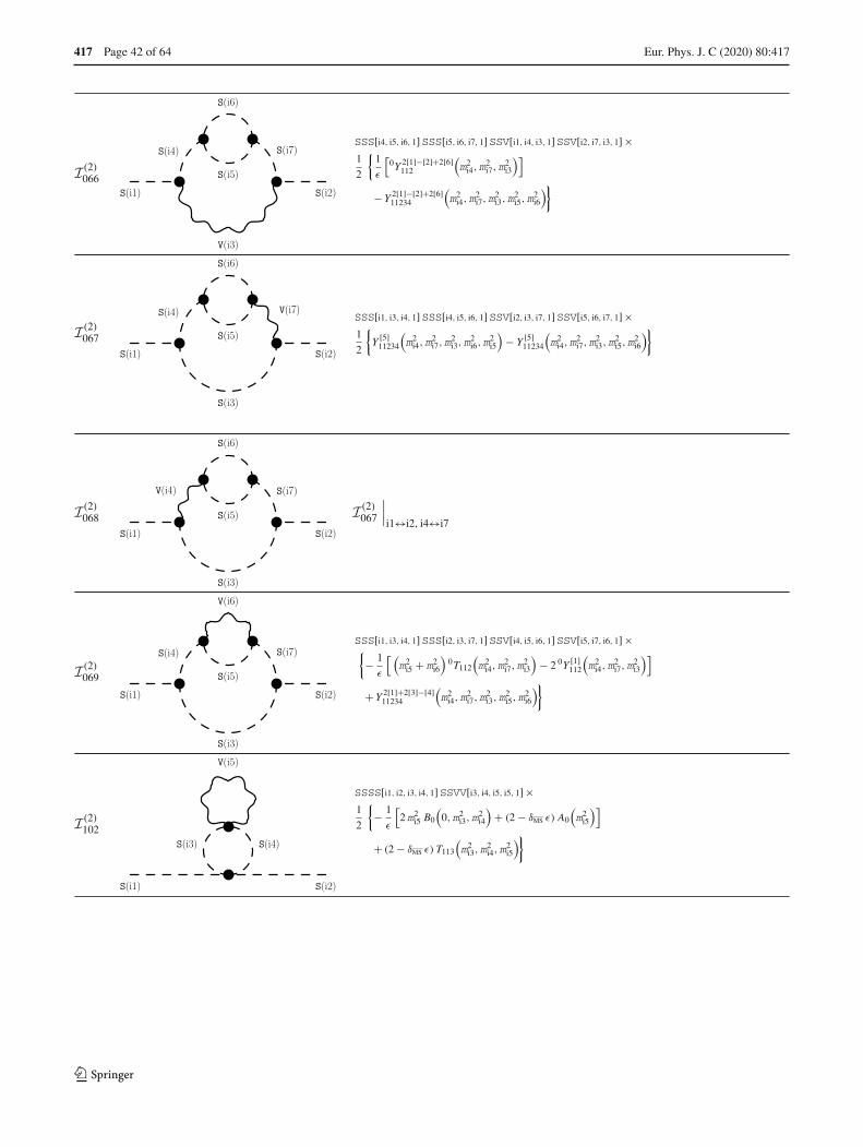
417 Page 42 of 64 Eur. Phys. J. C (2020) 80 :417
I(2)066
S(i1) S(i2)
V(i3)
S(i4)
S(i5)
S(i6)
S(i7)SSS[i4, i5, i6, 1]SSS[i5, i6, i7, 1]SSV[i1, i4, i3, 1]SSV[i2, i7, i3, 1]×1
2
{1
ε
[0Y 2[1]−[2]+2[6]
112
(m2
i4,m2i7,m
2i3
)]
− Y 2[1]−[2]+2[6]11234
(m2
i4,m2i7,m
2i3,m
2i5,m
2i6
)}
I(2)067
S(i1) S(i2)
S(i3)
S(i4)
S(i5)
S(i6)
V(i7)SSS[i1, i3, i4, 1]SSS[i4, i5, i6, 1]SSV[i2, i3, i7, 1]SSV[i5, i6, i7, 1]×1
2
{Y [5]
11234
(m2
i4,m2i7,m
2i3,m
2i6,m
2i5
)− Y [5]
11234
(m2
i4,m2i7,m
2i3,m
2i5,m
2i6
)}
I(2)068
S(i1) S(i2)
S(i3)
V(i4)
S(i5)
S(i6)
S(i7)
I(2)067
∣∣∣i1↔i2, i4↔i7
I(2)069
S(i1) S(i2)
S(i3)
S(i4)
S(i5)
V(i6)
S(i7)SSS[i1, i3, i4, 1]SSS[i2, i3, i7, 1]SSV[i4, i5, i6, 1]SSV[i5, i7, i6, 1]×{− 1
ε
[ (m2
i5 + m2i6
)0T112
(m2
i4,m2i7,m
2i3
)− 2 0Y [1]
112
(m2
i4,m2i7,m
2i3
)]
+ Y 2[1]+2[3]−[4]11234
(m2
i4,m2i7,m
2i3,m
2i5,m
2i6
)}
I(2)102
S(i1) S(i2)
S(i3) S(i4)
V(i5)
SSSS[i1, i2, i3, i4, 1]SSVV[i3, i4, i5, i5, 1]×1
2
{− 1
ε
[2m2
i5 B0
(0,m2
i3,m2i4
)+ (2 − δMS ε) A0
(m2
i5
)]
+ (2 − δMS ε) T113
(m2
i3,m2i4,m
2i5
)}
123

Eur. Phys. J. C (2020) 80 :417 Page 43 of 64 417
I(2)113
S(i1) S(i2)
S(i3)
V(i4)
S(i5) S(i6)
SSSS[i1, i2, i5, i6, 1]SSV[i3, i5, i4, 1]SSV[i3, i6, i4, 1]×1
2
{1
ε
[A0
(m2
i3
)+ 2 (2 − δMS ε) A0
(m2
i4
)+
(m2
i3 + m2i4
)B0
(0,m2
i5,m2i6
)
+ 2 0Y [1]11
(m2
i5,m2i6
)]
− Y 2[1]+2[3]−[4]1134
(m2
i5,m2i6,m
2i3,m
2i4
)}
B.2.4 Known results with fermions and one vector
I(2)028
S(i1) S(i2)
F(i3) F(i4)
V(i5)
F(i6) F(i7)
mi3 mi4 mi6 mi7 e[FFS[i3, i6, i1, 1]FFS[i4, i7, i2, 2]FFV[i3, i4, i5, 2]FFV[i6, i7, i5, 2]] ×{(2 − δMS ε) T12345
(m2
i3,m2i6,m
2i5,m
2i4,m
2i7
)}
+mi3 mi4 e[FFS[i3, i6, i1, 1]FFS[i4, i7, i2, 2]FFV[i3, i4, i5, 2]FFV[i6, i7, i5, 1]] ×{− (1 − δMS ε) Y [2]−[3]+[5]
12345
(m2
i3,m2i6,m
2i5,m
2i4,m
2i7
)}
+mi3 mi7 e[FFS[i3, i6, i1, 1]FFS[i4, i7, i2, 1]FFV[i3, i4, i5, 2]FFV[i6, i7, i5, 1]] ×{− (1 − δMS ε) Y [1]−[3]+[5]−[6]
12345
(m2
i3,m2i6,m
2i5,m
2i4,m
2i7
)}
+mi3 mi6 e[FFS[i3, i6, i1, 1]FFS[i4, i7, i2, 1]FFV[i3, i4, i5, 2]FFV[i6, i7, i5, 2]] ×{− 4
εB0
(p2,m2
i3,m2i6
)+ (2 − δMS ε) Y [4]+[5]−[6]
12345
(m2
i3,m2i6,m
2i5,m
2i4,m
2i7
)}
+ e[FFS[i3, i6, i1, 1]FFS[i4, i7, i2, 2]FFV[i3, i4, i5, 1]FFV[i6, i7, i5, 1]] ×1
2
{− 2
ε
[2 0Y [1]+[2]−[6]
12
(m2
i3,m2i6
)+ (2 − δMS ε) A0
(m2
i5
)]
+ Y 2[14]−4[16]+[36]+[66]12345
(m2
i3,m2i6,m
2i5,m
2i4,m
2i7
)
+ (1 − δMS ε) Y 2[15]−[36]12345
(m2
i3,m2i6,m
2i5,m
2i4,m
2i7
)}
+ [(i3, i4) ↔ (i6, i7)] + [(i1, i3, i6) ↔ (i2, i4, i7)] + [(i1, i3, i4) ↔ (i2, i7, i6)]
123
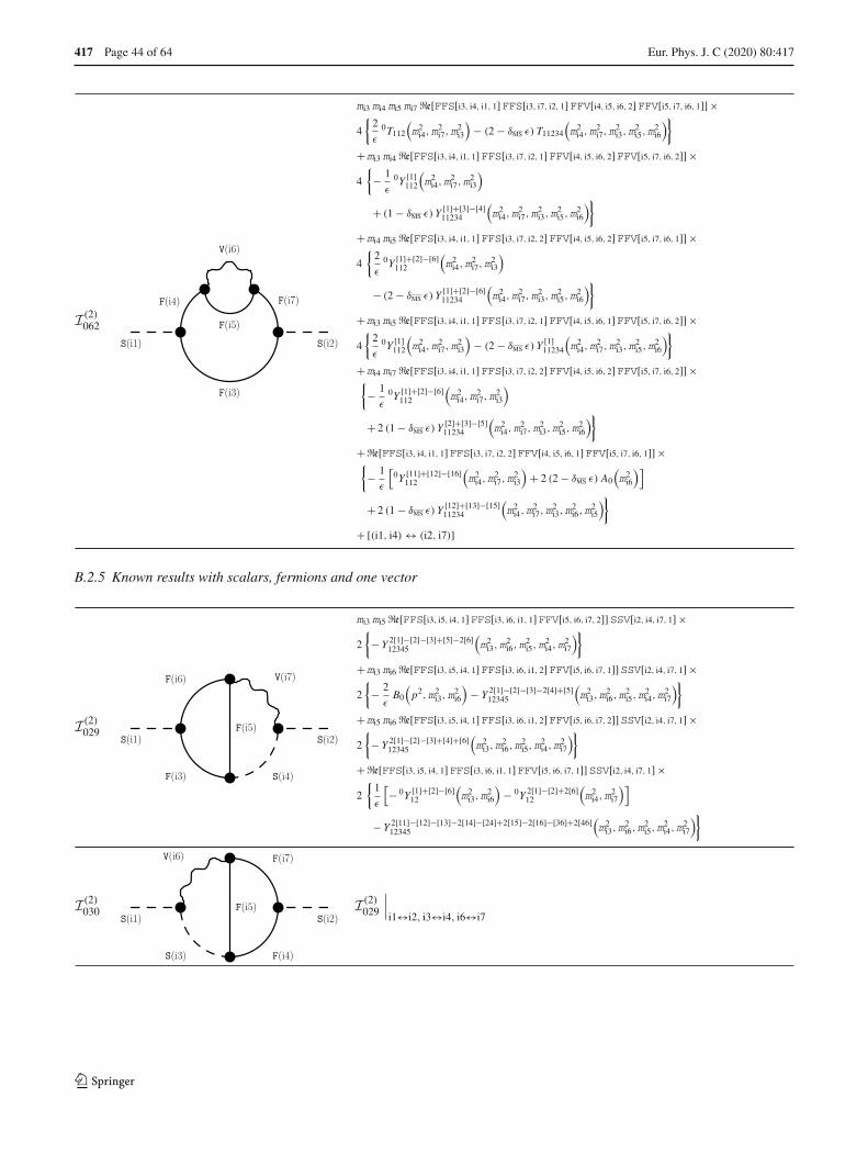
417 Page 44 of 64 Eur. Phys. J. C (2020) 80 :417
I(2)062
S(i1) S(i2)
F(i3)
F(i4)
F(i5)
V(i6)
F(i7)
mi3 mi4 mi5 mi7 e[FFS[i3, i4, i1, 1]FFS[i3, i7, i2, 1]FFV[i4, i5, i6, 2]FFV[i5, i7, i6, 1]] ×4
{2
ε
0T112
(m2
i4,m2i7,m
2i3
)− (2 − δMS ε) T11234
(m2
i4,m2i7,m
2i3,m
2i5,m
2i6
)}
+mi3 mi4 e[FFS[i3, i4, i1, 1]FFS[i3, i7, i2, 1]FFV[i4, i5, i6, 2]FFV[i5, i7, i6, 2]] ×4
{− 1
ε
0Y [1]112
(m2
i4,m2i7,m
2i3
)
+ (1 − δMS ε) Y [1]+[3]−[4]11234
(m2
i4,m2i7,m
2i3,m
2i5,m
2i6
)}
+mi4 mi5 e[FFS[i3, i4, i1, 1]FFS[i3, i7, i2, 2]FFV[i4, i5, i6, 2]FFV[i5, i7, i6, 1]] ×4
{2
ε
0Y [1]+[2]−[6]112
(m2
i4,m2i7,m
2i3
)
− (2 − δMS ε) Y [1]+[2]−[6]11234
(m2
i4,m2i7,m
2i3,m
2i5,m
2i6
)}
+mi3 mi5 e[FFS[i3, i4, i1, 1]FFS[i3, i7, i2, 1]FFV[i4, i5, i6, 1]FFV[i5, i7, i6, 2]] ×4
{2
ε
0Y [1]112
(m2
i4,m2i7,m
2i3
)− (2 − δMS ε) Y [1]
11234
(m2
i4,m2i7,m
2i3,m
2i5,m
2i6
)}
+mi4 mi7 e[FFS[i3, i4, i1, 1]FFS[i3, i7, i2, 2]FFV[i4, i5, i6, 2]FFV[i5, i7, i6, 2]] ×{− 1
ε
0Y [1]+[2]−[6]112
(m2
i4,m2i7,m
2i3
)
+ 2 (1 − δMS ε) Y [2]+[3]−[5]11234
(m2
i4,m2i7,m
2i3,m
2i5,m
2i6
)}
+ e[FFS[i3, i4, i1, 1]FFS[i3, i7, i2, 2]FFV[i4, i5, i6, 1]FFV[i5, i7, i6, 1]] ×{− 1
ε
[0Y [11]+[12]−[16]
112
(m2
i4,m2i7,m
2i3
)+ 2 (2 − δMS ε) A0
(m2
i6
)]
+ 2 (1 − δMS ε) Y [12]+[13]−[15]11234
(m2
i4,m2i7,m
2i3,m
2i6,m
2i5
)}
+ [(i1, i4) ↔ (i2, i7)]
B.2.5 Known results with scalars, fermions and one vector
I(2)029
S(i1) S(i2)
F(i3) S(i4)
F(i5)
F(i6) V(i7)
mi3 mi5 e[FFS[i3, i5, i4, 1]FFS[i3, i6, i1, 1]FFV[i5, i6, i7, 2]]SSV[i2, i4, i7, 1]×2
{− Y 2[1]−[2]−[3]+[5]−2[6]
12345
(m2
i3,m2i6,m
2i5,m
2i4,m
2i7
)}
+mi3 mi6 e[FFS[i3, i5, i4, 1]FFS[i3, i6, i1, 2]FFV[i5, i6, i7, 1]]SSV[i2, i4, i7, 1]×2
{− 2
εB0
(p2,m2
i3,m2i6
)− Y 2[1]−[2]−[3]−2[4]+[5]
12345
(m2
i3,m2i6,m
2i5,m
2i4,m
2i7
)}
+mi5 mi6 e[FFS[i3, i5, i4, 1]FFS[i3, i6, i1, 2]FFV[i5, i6, i7, 2]]SSV[i2, i4, i7, 1]×2
{− Y 2[1]−[2]−[3]+[4]+[6]
12345
(m2
i3,m2i6,m
2i5,m
2i4,m
2i7
)}
+e[FFS[i3, i5, i4, 1]FFS[i3, i6, i1, 1]FFV[i5, i6, i7, 1]]SSV[i2, i4, i7, 1]×2
{1
ε
[− 0Y [1]+[2]−[6]
12
(m2
i3,m2i6
)− 0Y 2[1]−[2]+2[6]
12
(m2
i4,m2i7
)]
− Y 2[11]−[12]−[13]−2[14]−[24]+2[15]−2[16]−[36]+2[46]12345
(m2
i3,m2i6,m
2i5,m
2i4,m
2i7
)}
I(2)030
S(i1) S(i2)
S(i3) F(i4)
F(i5)
V(i6) F(i7)
I(2)029
∣∣∣i1↔i2, i3↔i4, i6↔i7
123

Eur. Phys. J. C (2020) 80 :417 Page 45 of 64 417
I(2)063
S(i1) S(i2)
V(i3)
S(i4)
F(i5)
F(i6)
S(i7)
mi5 mi6 e[FFS[i5, i6, i4, 1]FFS[i5, i6, i7, 1]]SSV[i1, i4, i3, 1]SSV[i2, i7, i3, 1]×2
{− 1
ε
0Y 2[1]−[2]+2[6]112
(m2
i4,m2i7,m
2i3
)+ Y 2[1]−[2]+2[6]
11234
(m2
i4,m2i7,m
2i3,m
2i5,m
2i6
)}
+e[FFS[i5, i6, i4, 1]FFS[i5, i6, i7, 2]]SSV[i1, i4, i3, 1]SSV[i2, i7, i3, 1]×{
1
ε
[0Y 2[11]−[12]+2[16])
112
(m2
i4,m2i7,m
2i3
)
− 2(m2
i5 + m2i6
)0Y 2[1]−[2]+2[6]
112
(m2
i4,m2i7,m
2i3
)]
− Y ([1]−[3]−[4])(2[1]−[2]+2[6])11234
(m2
i4,m2i7,m
2i3,m
2i5,m
2i6
)}
I(2)064
S(i1) S(i2)
S(i3)
S(i4)
F(i5)
F(i6)
V(i7) mi5 e[FFS[i5, i6, i4, 1]FFV[i5, i6, i7, 2]]SSS[i1, i3, i4, 1]SSV[i2, i3, i7, 1]×{
1
ε
0Y [2]−[6]112
(m2
i4,m2i7,m
2i3
)− Y [1]−[3]−[4]+2[5]−2[6]
11234
(m2
i4,m2i7,m
2i3,m
2i5,m
2i6
)}
+ [i5 ↔ i6]
I(2)065
S(i1) S(i2)
S(i3)
V(i4)
F(i5)
F(i6)
S(i7)
I(2)064
∣∣∣i1↔i2, i4↔i7
B.2.6 New results with vectors
I(2)004
S(i1) S(i2)
S(i3)
V(i4) V(i5)
S(i6)
SSV[i1, i3, i4, 1]SSV[i2, i3, i5, 1]SSVV[i6, i6, i4, i5, 1]×1
2
{1
ε
[− A0
(m2
i6
)+ m2
i60Y [1]−2[2]−2[6]
112
(m2
i4,m2i5,m
2i3
)]
− Y [1]−2[2]−2[6]1123
(m2
i4,m2i5,m
2i3,m
2i6
)}
I(2)005
S(i1) S(i2)
V(i3)
S(i4) S(i5)
V(i6)
SSV[i1, i4, i3, 1]SSV[i2, i5, i3, 1]SSVV[i4, i5, i6, i6, 1]×{− 1
ε
[2m2
i60Y 2[1]−[2]+2[6]
112
(m2
i4,m2i5,m
2i3
)+ (2 − δMS ε) A0
(m2
i6
)]
+ (2 − δMS ε) Y 2[1]−[2]+2[6]1123
(m2
i4,m2i5,m
2i3,m
2i6
)}
123

417 Page 46 of 64 Eur. Phys. J. C (2020) 80 :417
I(2)006
S(i1) S(i2)
S(i3)
V(i4) V(i5)
V(i6)
SSV[i1, i3, i4, 1]SSV[i2, i3, i5, 1]×[4VVVV[i4, i5, i6, i6, 1] + VVVV[i4, i5, i6, i6, 2] + VVVV[i4, i5, i6, i6, 3]
]×
1
4
{1
ε
[− 2m2
i60Y [1]−2[2]−2[6]
112
(m2
i4,m2i5,m
2i3
)+ (2 − δMS ε) A0
(m2
i6
)]}
+SSV[i1, i3, i4, 1]SSV[i2, i3, i5, 1]×[(4 − 2 δMS ε)VVVV[i4, i5, i6, i6, 1] + VVVV[i4, i5, i6, i6, 2] + VVVV[i4, i5, i6, i6, 3]
]×
1
2
{Y [1]−2[2]−2[6]
1123
(m2
i4,m2i5,m
2i3,m
2i6
)}
I(2)007
S(i1) S(i2)
V(i3)
V(i4) V(i5)
S(i6)
SSVV[i6, i6, i4, i5, 1]SVV[i1, i3, i4, 1]SVV[i2, i3, i5, 1]×{− 1
ε(2 − δMS ε)m2
i60T112
(m2
i4,m2i5,m
2i3
)
+ (2 − δMS ε) T1123
(m2
i4,m2i5,m
2i3,m
2i6
)}
I(2)008
S(i1) S(i2)
V(i3)
V(i4) V(i5)
V(i6)
SVV[i1, i3, i4, 1]SVV[i2, i3, i5, 1]×[4VVVV[i4, i5, i6, i6, 1] + VVVV[i4, i5, i6, i6, 2] + VVVV[i4, i5, i6, i6, 3]
]×
{1
ε(2 − δMS ε)m2
i60T112
(m2
i4,m2i5,m
2i3
)}
SVV[i1, i3, i4, 1]SVV[i2, i3, i5, 1]×[(4 − 2 δMS ε)VVVV[i4, i5, i6, i6, 1] + VVVV[i4, i5, i6, i6, 2] + VVVV[i4, i5, i6, i6, 3]
]×
{− (2 − δMS ε) T1123
(m2
i4,m2i5,m
2i3,m
2i6
)}
I(2)011
S(i1) S(i2)
S(i3)
V(i4)
V(i5)
S(i6)
SSS[i1, i3, i6, 1]SSVV[i2, i6, i4, i5, 1]SVV[i3, i4, i5, 1]×{
2
εB0
(p2,m2
i3,m2i6
)− (2 − δMS ε) T1234
(m2
i3,m2i6,m
2i4,m
2i5
)}
I(2)017
S(i1) S(i2)
S(i3)
V(i4)
V(i5)
S(i6)
I(2)011
∣∣∣i1↔i2
123

Eur. Phys. J. C (2020) 80 :417 Page 47 of 64 417
I(2)012
S(i1) S(i2)
S(i3)
S(i4)
V(i5)
V(i6)
SSV[i1, i3, i6, 1]SSV[i3, i4, i5, 1]SSVV[i2, i4, i5, i6, 1]×1
4
{1
ε
[4 A0
(m2
i4
)+ 3 0Y 3[1]−[2]+[6]
12
(m2
i3,m2i6
)+ 4 (2 − δMS ε) A0
(m2
i5
)]
− 2 Y 4[1]−[2]−[3]+2[4]−[5]+2[6]1234
(m2
i3,m2i6,m
2i5,m
2i4
)}
I(2)018
S(i1) S(i2)
S(i3)
S(i4)
V(i5)
V(i6)
I(2)012
∣∣∣i1↔i2
I(2)013
S(i1) S(i2)
V(i3)
V(i4)
V(i5)
S(i6)
SSV[i1, i6, i3, 1]SSVV[i2, i6, i4, i5, 1]VVV[i3, i4, i5, 1]×1
2
{− 1
ε
3
2(2 − δMS ε)
[A0
(m2
i4
)− A0
(m2
i5
)]
− (3 − 2 δMS ε)[Y [5]
1234
(m2
i3,m2i6,m
2i5,m
2i4
)− Y [5]
1234
(m2
i3,m2i6,m
2i4,m
2i5
)]}
I(2)019
S(i1) S(i2)
V(i3)
V(i4)
V(i5)
S(i6)
I(2)013
∣∣∣i1↔i2
I(2)014
S(i1) S(i2)
V(i3)
S(i4)
V(i5)
V(i6)
SSVV[i2, i4, i5, i6, 1]SVV[i1, i3, i6, 1]SVV[i4, i3, i5, 1]×2
{− 1
ε(2 − δMS ε) B0
(p2,m2
i3,m2i6
)
+ (2 − δMS ε) T1234
(m2
i3,m2i6,m
2i4,m
2i5
)}
I(2)020
S(i1) S(i2)
V(i3)
S(i4)
V(i5)
V(i6)
I(2)014
∣∣∣i1↔i2
123

417 Page 48 of 64 Eur. Phys. J. C (2020) 80 :417
I(2)039
S(i1) S(i2)
S(i3) S(i4)
S(i5)
V(i6) V(i7)
SSS[i3, i4, i5, 1]SSV[i1, i3, i6, 1]SSV[i2, i4, i7, 1]SVV[i5, i6, i7, 1]×1
2
{Y 2[1]−[2]−[3]+2[4]−[5]+4[6]
12345
(m2
i3,m2i6,m
2i5,m
2i4,m
2i7
)}
I(2)040
S(i1) S(i2)
S(i3) V(i4)
S(i5)
S(i6) V(i7)
SSS[i1, i3, i6, 1]SSV[i3, i5, i4, 1]SSV[i5, i6, i7, 1]SVV[i2, i4, i7, 1]×1
4
{2
ε
[B0
(p2,m2
i3,m2i6
)+ 2 (2 − δMS ε) B0
(p2,m2
i4,m2i7
)]
− Y 2[1]+2[2]+4[3]−[4]−[5]−[6]12345
(m2
i3,m2i6,m
2i5,m
2i4,m
2i7
)}
I(2)042
S(i1) S(i2)
V(i3) S(i4)
S(i5)
V(i6) S(i7)
I(2)040
∣∣∣i1↔i2, i3↔i4, i6↔i7
I(2)041
S(i1) S(i2)
S(i3) V(i4)
S(i5)
V(i6) S(i7)
SSV[i1, i3, i6, 1]SSV[i2, i7, i4, 1]SSV[i3, i5, i4, 1]SSV[i5, i7, i6, 1]×{
1
ε
[− A0
(m2
i5
)− 0Y 2[1]−[2]+2[6]
12
(m2
i3,m2i6
)+ 0Y [1]−2[2]−2[6]
12
(m2
i4,m2i7
)]
+ Y ([1]−[2]+[3]−2[4]+[5]+[6])([1]−2[2]+[3]−[4]+[5]+[6])12345
(m2
i3,m2i6,m
2i5,m
2i4,m
2i7
)}
I(2)043
S(i1) S(i2)
S(i3) S(i4)
V(i5)
S(i6) V(i7)
SSS[i1, i3, i6, 1]SSV[i2, i4, i7, 1]SSV[i3, i4, i5, 1]SVV[i6, i5, i7, 1]×1
2
{− 2
εB0
(p2,m2
i3,m2i6
)+ Y 2[1]−[2]−[3]+4[4]−[5]+2[6]
12345
(m2
i3,m2i6,m
2i5,m
2i4,m
2i7
)}
I(2)044
S(i1) S(i2)
S(i3) S(i4)
V(i5)
V(i6) S(i7)
I(2)043
∣∣∣i1↔i2, i3↔i4, i6↔i7
I(2)047
S(i1) S(i2)
S(i3) V(i4)
S(i5)
V(i6) V(i7)
SSV[i1, i3, i6, 1]SSV[i3, i5, i4, 1]SVV[i2, i4, i7, 1]SVV[i5, i6, i7, 1]×1
2
{− 2
ε(2 − δMS ε) B0
(p2,m2
i4,m2i7
)
+ Y 5[1]−2[2]+[3]−2[4]+[5]+[6]12345
(m2
i3,m2i6,m
2i5,m
2i4,m
2i7
)}
123

Eur. Phys. J. C (2020) 80 :417 Page 49 of 64 417
I(2)048
S(i1) S(i2)
V(i3) S(i4)
S(i5)
V(i6) V(i7)
I(2)047
∣∣∣i1↔i2, i3↔i4, i6↔i7
I(2)049
S(i1) S(i2)
S(i3) S(i4)
V(i5)
V(i6) V(i7)
SSV[i1, i3, i6, 1]SSV[i2, i4, i7, 1]SSV[i3, i4, i5, 1]VVV[i5, i6, i7, 1]×1
2
{3
ε
0Y 2[1]−[2]+2[6]12
(m2
i3,m2i6
)
+ 2 Y 2[11]−2[12]−2[13]−[14]12345
(m2
i3,m2i6,m
2i5,m
2i4,m
2i7
)
+ 1
2Y 2[22]+4[23]+[33]+2[25]
12345
(m2
i3,m2i6,m
2i5,m
2i4,m
2i7
)
− 2 Y 2[16]+2[26]−[66]12345
(m2
i3,m2i6,m
2i5,m
2i4,m
2i7
)}
+ [(i1, i3, i6) ↔ (i2, i4, i7)]
I(2)050
S(i1) S(i2)
S(i3) V(i4)
V(i5)
S(i6) V(i7)
SSS[i1, i3, i6, 1]SVV[i2, i4, i7, 1]SVV[i3, i4, i5, 1]SVV[i6, i5, i7, 1]×{(2 − δMS ε) T12345
(m2
i3,m2i6,m
2i5,m
2i4,m
2i7
)}
I(2)052
S(i1) S(i2)
V(i3) S(i4)
V(i5)
V(i6) S(i7)
I(2)050
∣∣∣i1↔i2, i3↔i4, i6↔i7
I(2)051
S(i1) S(i2)
S(i3) V(i4)
V(i5)
V(i6) S(i7)
SSV[i1, i3, i6, 1]SSV[i2, i7, i4, 1]SVV[i3, i4, i5, 1]SVV[i7, i5, i6, 1]×1
2
{Y [1]−2[2]+[3]−2[4]+[5]+5[6]
12345
(m2
i3,m2i6,m
2i5,m
2i4,m
2i7
)}
I(2)053
S(i1) S(i2)
V(i3) V(i4)
S(i5)
V(i6) V(i7)
SVV[i1, i3, i6, 1]SVV[i2, i4, i7, 1]SVV[i5, i3, i4, 1]SVV[i5, i6, i7, 1]×{− (2 − δMS ε) T12345
(m2
i3,m2i6,m
2i5,m
2i4,m
2i7
)}
I(2)054
S(i1) S(i2)
S(i3) V(i4)
V(i5)
V(i6) V(i7)
SSV[i1, i3, i6, 1]SVV[i2, i4, i7, 1]SVV[i3, i4, i5, 1]VVV[i5, i6, i7, 1]×1
2
{3
ε(2 − δMS ε) B0
(p2,m2
i4,m2i7
)
− 2 (3 − 2 δMS ε) Y [1]−[2]+[3]−2[4]+[5]+[6]12345
(m2
i3,m2i6,m
2i5,m
2i4,m
2i7
)}
123

417 Page 50 of 64 Eur. Phys. J. C (2020) 80 :417
I(2)055
S(i1) S(i2)
V(i3) S(i4)
V(i5)
V(i6) V(i7)
I(2)054
∣∣∣i1↔i2, i3↔i4, i6↔i7
I(2)056
S(i1) S(i2)
V(i3) V(i4)
V(i5)
V(i6) V(i7)
SVV[i1, i3, i6, 1]SVV[i2, i4, i7, 1]VVV[i3, i4, i5, 1]VVV[i5, i6, i7, 1]×3
4
{6
ε(2 − δMS ε)
[B0
(p2,m2
i3,m2i6
)+ B0
(p2,m2
i4,m2i7
)]
− (3 − 2 δMS ε) Y [1]+[2]+2[3]+[4]+[5]−2[6]12345
(m2
i3,m2i6,m
2i5,m
2i4,m
2i7
)}
I(2)077
S(i1) S(i2)
V(i3)
S(i4)
S(i5)
S(i6)
V(i7)SSS[i4, i5, i6, 1]SSV[i1, i4, i3, 1]SSV[i5, i6, i7, 1]SVV[i2, i3, i7, 1]×1
4
{Y [5]
11234
(m2
i4,m2i7,m
2i3,m
2i6,m
2i5
)− Y [5]
11234
(m2
i4,m2i7,m
2i3,m
2i5,m
2i6
)
− 3 Y [3]−[4]11234
(m2
i4,m2i7,m
2i3,m
2i5,m
2i6
)}
I(2)078
S(i1) S(i2)
V(i3)
V(i4)
S(i5)
S(i6)
S(i7)
I(2)077
∣∣∣i1↔i2, i4↔i7
I(2)079
S(i1) S(i2)
S(i3)
V(i4)
S(i5)
S(i6)
V(i7)
SSV[i1, i3, i4, 1]SSV[i2, i3, i7, 1]SSV[i5, i6, i4, 1]SSV[i5, i6, i7, 1]×1
2
{1
ε
[16
0Y ([1]−[2]−[6])([1]−[2]−[6])−4[26]112
(m2
i4,m2i7,m
2i3
)
−m2i5
0Y [1]−2[2]−2[6]112
(m2
i4,m2i7,m
2i3
)+ A0
(m2
i5
)]
− Y [15]−[25]−[35]−[45]+2[55]−[56]11234
(m2
i4,m2i7,m
2i3,m
2i5,m
2i6
)}
+ [i5 ↔ i6]
I(2)080
S(i1) S(i2)
V(i3)
S(i4)
S(i5)
V(i6)
S(i7)
SSV[i1, i4, i3, 1]SSV[i2, i7, i3, 1]SSV[i4, i5, i6, 1]SSV[i5, i7, i6, 1]×{− 1
ε
[2 0Y 2[11]−[12]+2[16]
112
(m2
i4,m2i7,m
2i3
)
+(m2
i5 + m2i6
)0Y 2[1]−[2]+2[6]
112
(m2
i4,m2i7,m
2i3
)
+ A0
(m2
i5
)+ 2 (2 − δMS ε) A0
(m2
i6
)]
+ Y (2[1]+2[3]−[4])(2[1]−[2]+2[6])11234
(m2
i4,m2i7,m
2i3,m
2i5,m
2i6
)}
123

Eur. Phys. J. C (2020) 80 :417 Page 51 of 64 417
I(2)081
S(i1) S(i2)
S(i3)
S(i4)
S(i5)
V(i6)
V(i7)
SSS[i1, i3, i4, 1]SSV[i2, i3, i7, 1]SSV[i4, i5, i6, 1]SVV[i5, i6, i7, 1]×1
2
{3
ε
0Y [2]−[6]112
(m2
i4,m2i7,mi3
)
+ Y [5]11234
(m2
i4,m2i7,m
2i3,m
2i5,m
2i6
)− Y [5]
11234
(m2
i4,m2i7,m
2i3,m
2i6,m
2i5
)
− 3 Y [2]−[6]11234
(m2
i4,m2i7,m
2i3,m
2i5,m
2i6
)}
I(2)082
S(i1) S(i2)
S(i3)
V(i4)
S(i5)
V(i6)
S(i7)
I(2)081
∣∣∣i1↔i2, i4↔i7
I(2)083
S(i1) S(i2)
S(i3)
S(i4)
V(i5)
V(i6)
S(i7) SSS[i1, i3, i4, 1]SSS[i2, i3, i7, 1]SVV[i4, i5, i6, 1]SVV[i7, i5, i6, 1]×{
2
ε
0T112
(m2
i4,m2i7,m
2i3
)− (2 − δMS ε) T11234
(m2
i4,m2i7,m
2i3,m
2i5,m
2i6
)}
I(2)088
S(i1) S(i2)
V(i3)
V(i4)
S(i5)
S(i6)
V(i7)
SSV[i5, i6, i4, 1]SSV[i5, i6, i7, 1]SVV[i1, i3, i4, 1]SVV[i2, i3, i7, 1]×1
2
{1
ε
[2 (2 − δMS ε)
(m2
i5 + m2i6
)0T112
(m2
i4,m2i7,m
2i3
)
− 13 (3 − 2 δMS ε) 0Y [1]
112
(m2
i4,m2i7,m
2i3
)]
+ Y [1]−2[3]−2[4]11234
(m2
i4,m2i7,m
2i3,m
2i5,m
2i6
)}
I(2)089
S(i1) S(i2)
V(i3)
S(i4)
S(i5)
V(i6)
V(i7)
SSV[i1, i4, i3, 1]SSV[i4, i5, i6, 1]SVV[i2, i3, i7, 1]SVV[i5, i6, i7, 1]×1
4
{− 3
ε
[0Y 3[1]−[2]+[6]
112
(m2
i4,m2i7,m
2i3
)]
+ Y [5]11234
(m2
i4,m2i7,m
2i3,m
2i5,m
2i6
)− Y [5]
11234
(m2
i4,m2i7,m
2i3,m
2i6,m
2i5
)
+ 3 Y 3[1]−[2]+[3]−[4]+[6]11234
(m2
i4,m2i7,m
2i3,m
2i5,m
2i6
)}
123

417 Page 52 of 64 Eur. Phys. J. C (2020) 80 :417
I(2)090
S(i1) S(i2)
V(i3)
V(i4)
S(i5)
V(i6)
S(i7)
I(2)089
∣∣∣i1↔i2, i4↔i7
I(2)091
S(i1) S(i2)
S(i3)
V(i4)
S(i5)
V(i6)
V(i7)SSV[i1, i3, i4, 1]SSV[i2, i3, i7, 1]SVV[i5, i4, i6, 1]SVV[i5, i6, i7, 1]×{− 1
ε
0Y [1]−2[2]−2[6]112
(m2
i4,m2i7,m
2i3
)
+ Y [1]−2[2]−2[6]11234
(m2
i4,m2i7,m
2i3,m
2i5,m
2i6
)}
I(2)092
S(i1) S(i2)
V(i3)
S(i4)
V(i5)
V(i6)
S(i7)SSV[i1, i4, i3, 1]SSV[i2, i7, i3, 1]SVV[i4, i5, i6, 1]SVV[i7, i5, i6, 1]×{
2
ε
0Y 2[1]−[2]+2[6]112
(m2
i4,m2i7,m
2i3
)
− (2 − δMS ε) Y 2[1]−[2]+2[6]11234
(m2
i4,m2i7,m
2i3,m
2i5,m
2i6
)}
I(2)093
S(i1) S(i2)
S(i3)
S(i4)
V(i5)
V(i6)
V(i7) SSS[i1, i3, i4, 1]SSV[i2, i3, i7, 1]SVV[i4, i5, i6, 1]VVV[i5, i6, i7, 1]×1
2
{(3 − 2 δMS ε) Y [5]
11234
(m2
i4,m2i7,m
2i3,m
2i5,m
2i6
)}
+ [i5 ↔ i6]
I(2)094
S(i1) S(i2)
S(i3)
V(i4)
V(i5)
V(i6)
S(i7)
I(2)093
∣∣∣i1↔i2, i4↔i7
123
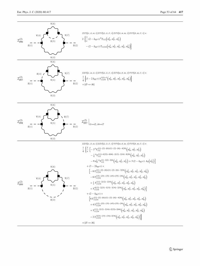
Eur. Phys. J. C (2020) 80 :417 Page 53 of 64 417
I(2)096
S(i1) S(i2)
V(i3)
V(i4)
S(i5)
V(i6)
V(i7)SVV[i1, i3, i4, 1]SVV[i2, i3, i7, 1]SVV[i5, i4, i6, 1]SVV[i5, i6, i7, 1]×2
{1
ε(2 − δMS ε) 0T112
(m2
i4,m2i7,m
2i3
)
− (2 − δMS ε) T11234
(m2
i4,m2i7,m
2i3,m
2i5,m
2i6
)}
I(2)097
S(i1) S(i2)
V(i3)
S(i4)
V(i5)
V(i6)
V(i7) SSV[i1, i4, i3, 1]SVV[i2, i3, i7, 1]SVV[i4, i5, i6, 1]VVV[i5, i6, i7, 1]×1
4
{(3 − 2 δMS ε) Y 3[3]+5
11234
(m2
i4,m2i7,m
2i3,m
2i5,m
2i6
)}
+ [i5 ↔ i6]
I(2)098
S(i1) S(i2)
V(i3)
V(i4)
V(i5)
V(i6)
S(i7)
I(2)097
∣∣∣i1↔i2, i4↔i7
I(2)099
S(i1) S(i2)
S(i3)
V(i4)
V(i5)
V(i6)
V(i7)
SSV[i1, i3, i4, 1]SSV[i2, i3, i7, 1]VVV[i4, i5, i6, 1]VVV[i5, i6, i7, 1]×1
4
{1
ε
[− 3 0Y ([1]−[2]−[6])([1]−[2]−[6])−4[26]
112
(m2
i4,m2i7,m
2i3
)
− 16
0Y [11]+4[22]+4[66]−2[12]−2[16]−8[26]112
(m2
i4,m2i7,m
2i3
)
− 9m2i5
0Y [1]−2[2]−2[6]112
(m2
i4,m2i7,m
2i3
)+ 3 (2 − δMS ε) A0
(m2
i5
)]
+ (3 − 2δMS ε)×[− 6 Y ([1]−[2]−[6])([1]−[2]−[6])−3[26]
11234
(m2
i4,m2i7,m
2i3,m
2i5,m
2i6
)
− 6 Y [15]−[25]−[35]−[45]+[55]−[56]11234
(m2
i4,m2i7,m
2i3,m
2i5,m
2i6
)
+ 12 Y [11]−2[12]−2[16]
11234
(m2
i4,m2i7,m
2i3,m
2i5,m
2i6
)
+ Y 4[13]−2[23]−3[33]−3[34]−2[36]11234
(m2
i4,m2i7,m
2i3,m
2i5,m
2i6
)]
+ (2 − δMS ε) ×[8 Y ([1]−[2]−[6])([1]−[2]−[6])−4[26]
11234
(m2
i4,m2i7,m
2i3,m
2i5,m
2i6
)
+ 4 Y [15]−[25]−[35]−[45]+[55]−[56]11234
(m2
i4,m2i7,m
2i3,m
2i5,m
2i6
)
+ Y [11]−2[12]−2[16]+2[22]+2[66]11234
(m2
i4,m2i7,m
2i3,m
2i5,m
2i6
)
− 2 Y 2[23]−[33]−[34]+2[36]11234
(m2
i4,m2i7,m
2i3,m
2i5,m
2i6
)]}
+ [i5 ↔ i6]
123

417 Page 54 of 64 Eur. Phys. J. C (2020) 80 :417
I(2)100
S(i1) S(i2)
V(i3)
V(i4)
V(i5)
V(i6)
V(i7)
SVV[i1, i3, i4, 1]SVV[i2, i3, i7, 1]VVV[i4, i5, i6, 1]VVV[i5, i6, i7, 1]×1
2
{1
ε
[(2 − δMS ε)
[9
(m2
i5 + m2i6
)0T112
(m2
i4,m2i7,m
2i3
)− 0Y [1]
112
(m2
i4,m2i7,m
2i3
)]
+ 113 (3 − 2 δMS ε) 0Y [1]
112
(m2
i4,m2i7,m
2i3
)]
− 3 (3 − 2 δMS ε) Y [1]+[3]+[4]11234
(m2
i4,m2i7,m
2i3,m
2i5,m
2i6
)}
I(2)103
S(i1) S(i2)
V(i3) V(i4)
S(i5)
SSVV[i1, i2, i3, i4, 1]SSVV[i5, i5, i3, i4, 1]×1
2
{1
ε
[2 A0
(m2
i5
)+ (2 − δMS ε)m2
i5 B0
(0,m2
i3,m2i4
)]
− (2 − δMS ε) T113
(m2
i3,m2i4,m
2i5
)}
I(2)104
S(i1) S(i2)
V(i3) V(i4)
V(i5) SSVV[i1, i2, i3, i4, 1]×[4VVVV[i3, i4, i5, i5, 1] + VVVV[i3, i4, i5, i5, 2] + VVVV[i3, i4, i5, i5, 3]
]×
1
2
{− 1
ε(2 − δMS ε)
[A0
(m2
i5
)+ m2
i5 B0
(0,m2
i3,m2i4
)]}
+SSVV[i1, i2, i3, i4, 1]×[(4 − 2 δMS ε)VVVV[i3, i4, i5, i5, 1] + VVVV[i3, i4, i5, i5, 2] + VVVV[i3, i4, i5, i5, 3]
]×
1
2
{(2 − δMS ε) T113
(m2
i3,m2i4,m
2i5
)}
I(2)106
S(i1) S(i2)
S(i3)
S(i4)
V(i5)
V(i6)SSS[i1, i3, i4, 1]SSVV[i3, i4, i5, i6, 1]SVV[i2, i5, i6, 1]×1
2
{1
ε
[2 B0
(p2,m2
i3,m2i4
)+ (2 − δMS ε) B0
(p2,m2
i5,m2i6
)]
− (2 − δMS ε) T1245
(m2
i3,m2i4,m
2i5,m
2i6
)}
I(2)108
S(i1) S(i2)
V(i3)
V(i4)
S(i5)
S(i6)
I(2)106
∣∣∣i1↔i2, i3↔i5, i4↔i6
I(2)107
S(i1) S(i2)
S(i3)
V(i4)
S(i5)
V(i6)SSV[i1, i3, i4, 1]SSV[i2, i5, i6, 1]SSVV[i3, i5, i4, i6, 1]×1
4
{− 3
ε
0Y [1]−[2]+3[6]12
(m2
i3,m2i4
)+ Y 4[1]−2[2]−[3]+4[6]
1245
(m2
i3,m2i4,m
2i5,m
2i6
)}
+ [(i1, i3, i4) ↔ (i2, i5, i6)]
I(2)109
S(i1) S(i2)
V(i3)
V(i4)
V(i5)
V(i6)
SVV[i1, i3, i4, 1]SVV[i2, i5, i6, 1]×[4VVVV[i3, i4, i5, i6, 1] + VVVV[i3, i4, i5, i6, 2] + VVVV[i3, i4, i5, i6, 3]
]×
1
2
{1
ε(2 − δMS ε)
[B0
(p2,m2
i3,m2i4
)+ B0
(p2,m2
i5,m2i6
)] }
+SVV[i1, i3, i4, 1]SVV[i2, i5, i6, 1]×[(4 − 2 δMS ε)VVVV[i3, i4, i5, i6, 1] + VVVV[i3, i4, i5, i6, 2] + VVVV[i3, i4, i5, i6, 3]
]×
1
2
{− (2 − δMS ε) T1245
(m2
i3,m2i4,m
2i5,m
2i6
)}
123

Eur. Phys. J. C (2020) 80 :417 Page 55 of 64 417
I(2)115
S(i1) S(i2)
S(i3)
S(i4)
V(i5) V(i6)
SSV[i3, i4, i5, 1]SSV[i3, i4, i6, 1]SSVV[i1, i2, i5, i6, 1]×1
4
{1
ε
[− A0
(m2
i3
)− A0
(m2
i4
)+ 1
3 (3 − 2 δMS ε) 0Y [1]11
(m2
i5,m2i6
)
− (2 − δMS ε)(m2
i3 + m2i4
)B0
(0,m2
i5,m2i6
)]
− Y [1]−2[3]−2[4]1134
(m2
i5,m2i6,m
2i3,m
2i4
)}
I(2)116
S(i1) S(i2)
V(i3)
V(i4)
S(i5) S(i6)
SSSS[i1, i2, i5, i6, 1]SVV[i5, i3, i4, 1]SVV[i6, i3, i4, 1]×1
2
{2
εB0
(0,m2
i5,m2i6
)− (2 − δMS ε) T1134
(m2
i5,m2i6,m
2i3,m
2i4
)}
I(2)118
S(i1) S(i2)
S(i3)
V(i4)
V(i5) V(i6)
SSVV[i1, i2, i5, i6, 1]SVV[i3, i4, i5, 1]SVV[i3, i4, i6, 1]×{− 1
ε(2 − δMS ε) B0
(0,m2
i5,m2i6
)+ (2 − δMS ε) T1134
(m2
i5,m2i6,m
2i3,m
2i4
)}
I(2)119
S(i1) S(i2)
V(i3)
V(i4)
V(i5) V(i6)
SSVV[i1, i2, i5, i6, 1]VVV[i3, i4, i5, 1]VVV[i3, i4, i6, 1]×1
4
{−1
ε
[(2 − δMS ε)
[9 A0
(m2
i3
)+ 9 A0
(m2
i4
)− 0Y [1]
11
(m2
i5,m2i6
)
+ 9(m2
i3 + m2i4
)B0
(0,m2
i5,m2i6
)]
113 (3 − 2 δMS ε) 0Y [1]
11
(m2
i5,m2i6
)]
+ 3 (3 − 2 δMS ε) Y [1]+[3]+[4]1134
(m2
i5,m2i6,m
2i3,m
2i4
)}
I(2)121
S(i1) S(i2)
S(i3)
V(i4)
V(i5)
SSVV[i1, i3, i4, i5, 1]SSVV[i2, i3, i4, i5, 1]×{
1
ε
[2 A0
(m2
i3
)+ (2 − δMS ε)
[A0
(m2
i4
)+ A0
(m2
i5
)]]
− (2 − δMS ε) T234
(m2
i3,m2i4,m
2i5
)}
123

417 Page 56 of 64 Eur. Phys. J. C (2020) 80 :417
B.2.7 New results with fermions and vectors
I(2)037
S(i1) S(i2)
F(i3) V(i4)
F(i5)
F(i6) V(i7)
mi3 mi5 mi6 e[FFS[i3, i6, i1, 1]FFV[i3, i5, i4, 2]FFV[i5, i6, i7, 1]]SVV[i2, i4, i7, 1]×2
{(2 − δMS ε) T12345
(m2
i3,m2i6,m
2i5,m
2i4,m
2i7
)}
+mi3 e[FFS[i3, i6, i1, 1]FFV[i3, i5, i4, 2]FFV[i5, i6, i7, 2]]SVV[i2, i4, i7, 1]×2
{1
ε(2 − δMS ε) B0
(p2,m2
i4,m2i7
)
− (1 − δMS ε) Y [2]+[3]−[5]12345
(m2
i3,m2i6,m
2i5,m
2i4,m
2i7
)}
+mi5 e[FFS[i3, i6, i1, 1]FFV[i3, i5, i4, 1]FFV[i5, i6, i7, 2]]SVV[i2, i4, i7, 1]×{− 2
ε(2 − δMS ε) B0
(p2,m2
i4,m2i7
)
+ (2 − δMS ε) Y [1]+[2]−[6]12345
(m2
i3,m2i6,m
2i5,m
2i4,m
2i7
)}
+ [(i3, i4) ↔ (i6, i7)]
I(2)038
S(i1) S(i2)
V(i3) F(i4)
F(i5)
V(i6) F(i7)
I(2)037
∣∣∣i1↔i2, i3↔i4, i6↔i7
I(2)074
S(i1) S(i2)
V(i3)
S(i4)
F(i5)
F(i6)
V(i7)
mi5 e[FFS[i5, i6, i4, 1]FFV[i5, i6, i7, 2]]SSV[i1, i4, i3, 1]SVV[i2, i3, i7, 1]×1
2
{− 1
ε
0Y 3[1]−[2]+[6]112
(m2
i4,m2i7,m
2i3
)
+ Y 3[1]−[2]−3[3]+3[4]+[6]11234
(m2
i4,m2i7,m
2i3,m
2i5,m
2i6
)
+ Y [5]11234
(m2
i4,m2i7,m
2i3,m
2i6,m
2i5
)− Y [5]
11234
(m2
i4,m2i7,m
2i3,m
2i5,m
2i6
)}
+ [i5 ↔ i6]
I(2)075
S(i1) S(i2)
V(i3)
V(i4)
F(i5)
F(i6)
S(i7)
I(2)074
∣∣∣i1↔i2, i4↔i7
I(2)076
S(i1) S(i2)
S(i3)
V(i4)
F(i5)
F(i6)
V(i7)
mi5 mi6 e[FFV[i5, i6, i4, 1]FFV[i5, i6, i7, 1]]SSV[i1, i3, i4, 1]SSV[i2, i3, i7, 1]×{
1
ε
0Y [1]−2[2]−2[6]112
(m2
i4,m2i7,m
2i3
)− Y [1]−2[2]−2[6]
11234
(m2
i4,m2i7,m
2i3,m
2i5,m
2i6
)}
+ e[FFV[i5, i6, i4, 1]FFV[i5, i6, i7, 2]]SSV[i1, i3, i4, 1]SSV[i2, i3, i7, 1]×{− 1
ε
[m2
i50Y [1]−2[2]−2[6]
112
(m2
i4,m2i7,m
2i3
)
+ 13
0Y ([1]−[2]−[6])([1]−[2]−[6])−4[26]112
(m2
i4,m2i7,m
2i3
)]
− Y [13]−[33]−[34]−2[26]11234
(m2
i4,m2i7,m
2i3,m
2i5,m
2i6
)
+ 2 Y [15]−[25]−[35]−[45]+[55]−[56]11234
(m2
i4,m2i7,m
2i3,m
2i5,m
2i6
)}
+ [i5 ↔ i6]
123

Eur. Phys. J. C (2020) 80 :417 Page 57 of 64 417
I(2)087
S(i1) S(i2)
V(i3)
V(i4)
F(i5)
F(i6)
V(i7)
mi5 mi6 e[FFV[i5, i6, i4, 1]FFV[i5, i6, i7, 1]]SVV[i1, i3, i4, 1]SVV[i2, i3, i7, 1]×2
{− 1
ε(2 − δMS ε) 0T112
(m2
i4,m2i7,m
2i3
)
+ (2 − δMS ε) T11234
(m2
i4,m2i7,m
2i3,m
2i5,m
2i6
)}
+ e[FFV[i5, i6, i4, 1]FFV[i5, i6, i7, 2]]SVV[i1, i3, i4, 1]SVV[i2, i3, i7, 1]×{
1
ε
[2 (2 − δMS ε)m2
i50T112
(m2
i4,m2i7,m
2i3
)
− 13 (3 − 2 δMS ε) 0Y [1]
112
(m2
i4,m2i7,m
2i3
)]
+ (1 − δMS ε) Y [1]−2[3]11234
(m2
i4,m2i7,m
2i3,m
2i5,m
2i6
)}
+ [i5 ↔ i6]
I(2)114
S(i1) S(i2)
F(i3)
F(i4)
V(i5) V(i6)
mi3 mi4 e[FFV[i3, i4, i5, 1]FFV[i3, i4, i6, 1]]SSVV[i1, i2, i5, i6, 1]×{
1
ε(2 − δMS ε) B0
(0,m2
i5,m2i6
)− (2 − δMS ε) T1134
(m2
i5,m2i6,m
2i3,m
2i4
)}
+ e[FFV[i3, i4, i5, 1]FFV[i3, i4, i6, 2]]SSVV[i1, i2, i5, i6, 1]×1
2
{1
ε
[13 (3 − 2 δMS ε) 0Y [1]
11
(m2
i5,m2i6
)− 2 (2 − δMS ε)m2
i3 B0
(0,m2
i5,m2i6
)]
− (1 − δMS ε) Y [1]−2[3]1134
(m2
i5,m2i6,m
2i3,m
2i4
)}
+ [i5 ↔ i6]
B.2.8 New results with ghosts
I(2)025
S(i1) S(i2)
S(i3) U(i4)
U(i5)
S(i6) U(i7)
SSS[i1, i3, i6, 1]SUU[i2,−i7, i4, 1]SUU[i3,−i4, i5, 1]SUU[i6,−i5, i7, 1]×1
2
{T12345
(m2
i3,m2i6,m
2i5,m
2i4,m
2i7
)}
I(2)026
S(i1) S(i2)
U(i3) S(i4)
U(i5)
U(i6) S(i7)
I(2)025
∣∣∣i1↔i2, i3↔i4, i6↔i7
I(2)027
S(i1) S(i2)
U(i3) U(i4)
S(i5)
U(i6) U(i7)
SUU[i1,−i3, i6, 1]SUU[i2,−i7, i4, 1]SUU[i5,−i4, i3, 1]SUU[i5,−i6, i7, 1]×1
2
{T12345
(m2
i3,m2i6,m
2i5,m
2i4,m
2i7
)}
I(2)034
S(i1) S(i2)
S(i3) U(i4)
U(i5)
V(i6) U(i7)SSV[i1, i3, i6, 1]SUU[i2,−i7, i4, 1]SUU[i3,−i4, i5, 1]UUV[−i5, i7, i6, 1]×1
2
{2
εB0
(p2,m2
i7,m2i4
)− Y 2[1]−[2]+[3]−2[4]+[5]
12345
(m2
i3,m2i6,m
2i5,m
2i4,m
2i7
)}
+SSV[i1, i3, i6, 1]SUU[i2, i7,−i4, 1]SUU[i3, i4,−i5, 1]UUV[i5,−i7, i6, 2]×1
2
{− Y [2]−[3]+2[4]−[5]−2[6]
12345
(m2
i3,m2i6,m
2i5,m
2i4,m
2i7
)}
123

417 Page 58 of 64 Eur. Phys. J. C (2020) 80 :417
I(2)035
S(i1) S(i2)
U(i3) S(i4)
U(i5)
U(i6) V(i7)
I(2)034
∣∣∣i1↔i2, i3↔i4, i6↔i7
I(2)036
S(i1) S(i2)
U(i3) U(i4)
V(i5)
U(i6) U(i7)
SUU[i1,−i3, i6, 1]SUU[i2,−i7, i4, 1]UUV[−i4, i3, i5, 1]UUV[−i6, i7, i5, 1]×1
2
{− Y [1]−[3]+[5]−[6]
12345
(m2
i3,m2i6,m
2i5,m
2i4,m
2i7
)}
I(2)045
S(i1) S(i2)
U(i3) V(i4)
U(i5)
U(i6) V(i7)
SUU[i1,−i6, i3, 1]SVV[i2, i4, i7, 1]UUV[−i3, i5, i4, 1]UUV[−i5, i6, i7, 1]×1
2
{− 1
ε(2 − δMS ε) B0
(p2,m2
i4,m2i7
)
+ Y [1]+[3]−[4]12345
(m2
i3,m2i6,m
2i5,m
2i4,m
2i7
)}
I(2)046
S(i1) S(i2)
V(i3) U(i4)
U(i5)
V(i6) U(i7)
I(2)045
∣∣∣i1↔i2, i3↔i4, i6↔i7
I(2)060
S(i1) S(i2)
S(i3)
S(i4)
U(i5)
U(i6)
S(i7)SSS[i1, i3, i4, 1]SSS[i2, i3, i7, 1]SUU[i4,−i5, i6, 1]SUU[i7,−i6, i5, 1]×1
2
{− 1
ε
0T112
(m2
i4,m2i7,m
2i3
)+ T11234
(m2
i4,m2i7,m
2i3,m
2i5,m
2i6
)}
I(2)061
S(i1) S(i2)
U(i3)
U(i4)
S(i5)
U(i6)
U(i7)SUU[i1,−i3, i4, 1]SUU[i2,−i7, i3, 1]SUU[i5,−i4, i6, 1]SUU[i5,−i6, i7, 1]×{− 1
ε
0T112
(m2
i4,m2i7,m
2i3
)+ T11234
(m2
i4,m2i7,m
2i3,m
2i5,m
2i6
)}
123

Eur. Phys. J. C (2020) 80 :417 Page 59 of 64 417
I(2)070
S(i1) S(i2)
V(i3)
S(i4)
U(i5)
U(i6)
S(i7)SSV[i1, i4, i3, 1]SSV[i2, i7, i3, 1]SUU[i4,−i5, i6, 1]SUU[i7,−i6, i5, 1]×1
2
{− 1
ε
0Y 2[1]−[2]+2[6]112
(m2
i4,m2i7,m
2i3
)
+ Y 2[1]−[2]+2[6]11234
(m2
i4,m2i7,m
2i3,m
2i5,m
2i6
)}
I(2)071
S(i1) S(i2)
S(i3)
S(i4)
U(i5)
U(i6)
V(i7)SSS[i1, i3, i4, 1]SSV[i2, i3, i7, 1]SUU[i4,−i5, i6, 1]UUV[−i6, i5, i7, 1]×1
2
{1
ε
0Y [2]−[6]112
(m2
i4,m2i7,m
2i3
)− Y [2]−[6]
11234
(m2
i4,m2i7,m
2i3,m
2i5,m
2i6
)
+ Y [5]11234
(m2
i4,m2i7,m
2i3,m
2i6,m
2i5
)− Y [5]
11234
(m2
i4,m2i7,m
2i3,m
2i5,m
2i6
)}
I(2)072
S(i1) S(i2)
S(i3)
V(i4)
U(i5)
U(i6)
S(i7)
I(2)071
∣∣∣i1↔i2, i4↔i7
I(2)073
S(i1) S(i2)
U(i3)
U(i4)
U(i5)
V(i6)
U(i7)
[SUU[i1,−i3, i4, 1]SUU[i2,−i7, i3, 1]UUV[−i4, i5, i6, 1]UUV[−i5, i7, i6, 1]+SUU[i1, i3,−i4, 1]SUU[i2, i7,−i3, 1]UUV[i4,−i5, i6, 2]UUV[i5,−i7, i6, 2]
]×
1
2
{1
ε
0Y [1]112
(m2
i4,m2i7,m
2i3
)− Y [1]+[3]−[4]
11234
(m2
i4,m2i7,m
2i3,m
2i5,m
2i6
)}
I(2)084
S(i1) S(i2)
V(i3)
S(i4)
U(i5)
U(i6)
V(i7)
SSV[i1, i4, i3, 1]SUU[i4,−i5, i6, 1]SVV[i2, i3, i7, 1]UUV[−i6, i5, i7, 1]×1
4
{− 1
ε
0Y 3[1]−[2]+[6]112
(m2
i4,m2i7,m
2i3
)
+ Y 3[1]−[2]−3[3]+3[4]+[6]11234
(m2
i4,m2i7,m
2i3,m
2i5,m
2i6
)
+ Y [5]11234
(m2
i4,m2i7,m
2i3,m
2i6,m
2i5
)− Y [5]
11234
(m2
i4,m2i7,m
2i3,m
2i5,m
2i6
)}
123
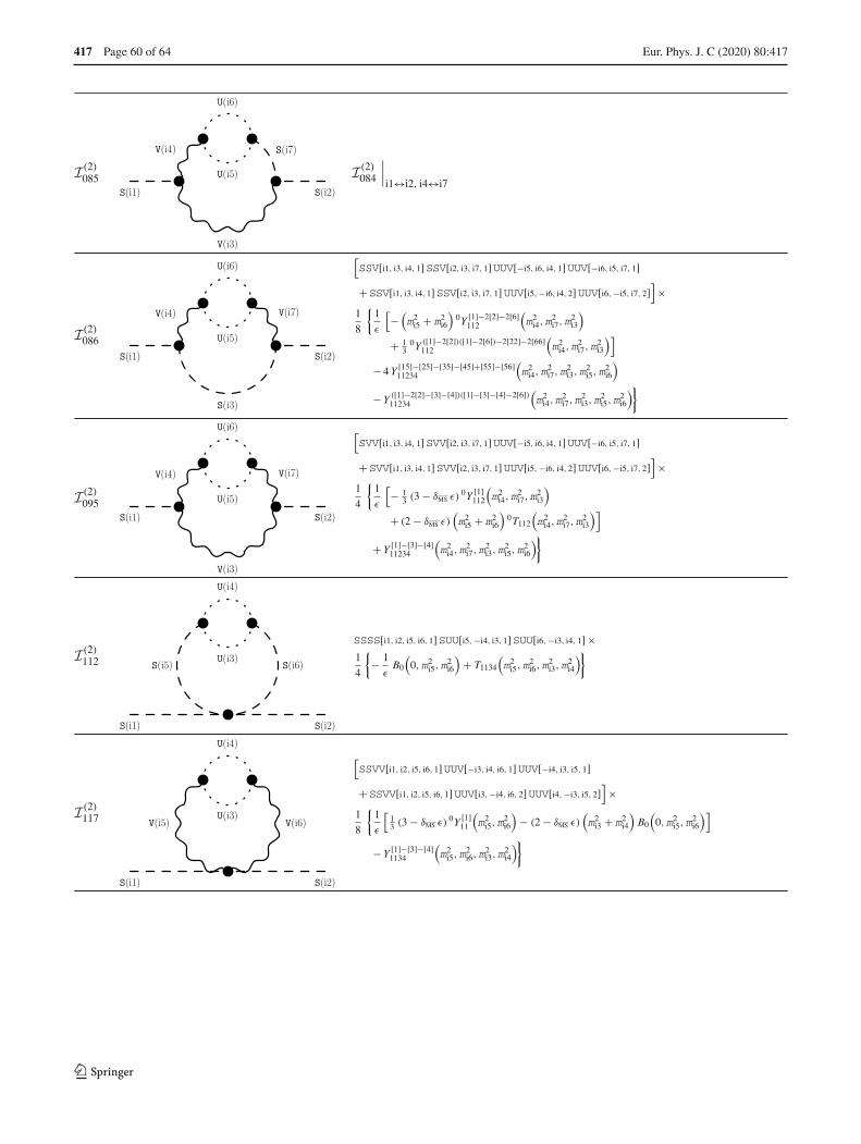
417 Page 60 of 64 Eur. Phys. J. C (2020) 80 :417
I(2)085
S(i1) S(i2)
V(i3)
V(i4)
U(i5)
U(i6)
S(i7)
I(2)084
∣∣∣i1↔i2, i4↔i7
I(2)086
S(i1) S(i2)
S(i3)
V(i4)
U(i5)
U(i6)
V(i7)
[SSV[i1, i3, i4, 1]SSV[i2, i3, i7, 1]UUV[−i5, i6, i4, 1]UUV[−i6, i5, i7, 1]+SSV[i1, i3, i4, 1]SSV[i2, i3, i7, 1]UUV[i5,−i6, i4, 2]UUV[i6,−i5, i7, 2]
]×
1
8
{1
ε
[−
(m2
i5 + m2i6
)0Y [1]−2[2]−2[6]
112
(m2
i4,m2i7,m
2i3
)
+ 13
0Y ([1]−2[2])([1]−2[6])−2[22]−2[66]112
(m2
i4,m2i7,m
2i3
)]
− 4 Y [15]−[25]−[35]−[45]+[55]−[56]11234
(m2
i4,m2i7,m
2i3,m
2i5,m
2i6
)
− Y ([1]−2[2]−[3]−[4])([1]−[3]−[4]−2[6])11234
(m2
i4,m2i7,m
2i3,m
2i5,m
2i6
)}
I(2)095
S(i1) S(i2)
V(i3)
V(i4)
U(i5)
U(i6)
V(i7)
[SVV[i1, i3, i4, 1]SVV[i2, i3, i7, 1]UUV[−i5, i6, i4, 1]UUV[−i6, i5, i7, 1]+SVV[i1, i3, i4, 1]SVV[i2, i3, i7, 1]UUV[i5,−i6, i4, 2]UUV[i6,−i5, i7, 2]
]×
1
4
{1
ε
[− 1
3 (3 − δMS ε) 0Y [1]112
(m2
i4,m2i7,m
2i3
)
+ (2 − δMS ε)(m2
i5 + m2i6
)0T112
(m2
i4,m2i7,m
2i3
)]
+ Y [1]−[3]−[4]11234
(m2
i4,m2i7,m
2i3,m
2i5,m
2i6
)}
I(2)112
S(i1) S(i2)
U(i3)
U(i4)
S(i5) S(i6)
SSSS[i1, i2, i5, i6, 1]SUU[i5,−i4, i3, 1]SUU[i6,−i3, i4, 1]×1
4
{− 1
εB0
(0,m2
i5,m2i6
)+ T1134
(m2
i5,m2i6,m
2i3,m
2i4
)}
I(2)117
S(i1) S(i2)
U(i3)
U(i4)
V(i5) V(i6)
[SSVV[i1, i2, i5, i6, 1]UUV[−i3, i4, i6, 1]UUV[−i4, i3, i5, 1]+SSVV[i1, i2, i5, i6, 1]UUV[i3,−i4, i6, 2]UUV[i4,−i3, i5, 2]
]×
1
8
{1
ε
[13 (3 − δMS ε) 0Y [1]
11
(m2
i5,m2i6
)− (2 − δMS ε)
(m2
i3 + m2i4
)B0
(0,m2
i5,m2i6
)]
− Y [1]−[3]−[4]1134
(m2
i5,m2i6,m
2i3,m
2i4
)}
123

Eur. Phys. J. C (2020) 80 :417 Page 61 of 64 417
References
1. G. Degrassi, S. Di Vita, J. Elias-Miro, J.R. Espinosa, G.F. Giudice,G. Isidori, A. Strumia, Higgs mass and vacuum stability in theStandard Model at NNLO. JHEP 08, 098 (2012). arXiv:1205.6497
2. D. Buttazzo, G. Degrassi, P.P. Giardino, G.F. Giudice, F. Sala, A.Salvio, A. Strumia, Investigating the near-criticality of the Higgsboson. JHEP 12, 089 (2013). arXiv:1307.3536
3. T. van Ritbergen, J.A.M. Vermaseren, S.A. Larin, The Four loopbeta function in quantum chromodynamics. Phys. Lett. B 400,379 (1997). arXiv:hep-ph/9701390
4. K.G. Chetyrkin, Quark mass anomalous dimension to O (alpha-s**4). Phys. Lett. B 404, 161 (1997). arXiv:hep-ph/9703278
5. J.A.M. Vermaseren, S.A. Larin, T. van Ritbergen, The four loopquark mass anomalous dimension and the invariant quark mass.Phys. Lett. B 405, 327 (1997). arXiv:hep-ph/9703284
6. K.G. Chetyrkin, Four-loop renormalization of QCD: Full setof renormalization constants and anomalous dimensions. Nucl.Phys. B 710, 499 (2005). arXiv:hep-ph/0405193
7. L.N. Mihaila, J. Salomon, M. Steinhauser, Gauge coupling betafunctions in the Standard Model to three loops. Phys. Rev. Lett.108, 151602 (2012). arXiv:1201.5868
8. K.G. Chetyrkin, M.F. Zoller, Three-loop β-functions for top-Yukawa and the Higgs self-interaction in the Standard Model.JHEP 06, 033 (2012). arXiv:1205.2892
9. L.N. Mihaila, J. Salomon, M. Steinhauser, Renormalization con-stants and beta functions for the gauge couplings of the Stan-dard Model to three-loop order. Phys. Rev. D 86, 096008 (2012).arXiv:1208.3357
10. A.V. Bednyakov, A.F. Pikelner, V.N. Velizhanin, Anomalousdimensions of gauge fields and gauge coupling beta-functionsin the Standard Model at three loops. JHEP 01, 017 (2013).arXiv:1210.6873
11. A.V. Bednyakov, A.F. Pikelner, V.N. Velizhanin, Yukawa couplingbeta-functions in the Standard Model at three loops. Phys. Lett.B 722, 336 (2013). arXiv:1212.6829
12. K.G. Chetyrkin, M.F. Zoller, β-function for the Higgsself-interaction in the Standard Model at three-loop level.JHEP 04, 091 (2013), arXiv:1303.2890 (erratum: JHEP 09, 155,2013)
13. A.V. Bednyakov, A.F. Pikelner, V.N. Velizhanin, Higgs self-coupling beta-function in the Standard Model at three loops. Nucl.Phys. B 875, 552 (2013). arXiv:1303.4364
14. P. Marquard, A.V. Smirnov, V.A. Smirnov, M. Steinhauser, Quarkmass relations to four-loop order in perturbative QCD. Phys. Rev.Lett. 114, 142002 (2015). arXiv:1502.01030
15. S.P. Martin, Four-loop Standard Model effective potential atleading order in QCD. Phys. Rev. D 92, 054029 (2015).arXiv:1508.00912
16. K.G. Chetyrkin, M.F. Zoller, Leading QCD-induced four-loopcontributions to the β-function of the Higgs self-coupling in theSM and vacuum stability. JHEP 06, 175 (2016). arXiv:1604.00853
17. S.P. Martin, D.G. Robertson, Higgs boson mass in the StandardModel at two-loop order and beyond. Phys. Rev. D 90, 073010(2014). arXiv:1407.4336
18. B.A. Kniehl, A.F. Pikelner, O.L. Veretin, Two-loop electroweakthreshold corrections in the Standard Model. Nucl. Phys. B 896,19 (2015). arXiv:1503.02138
19. B.A. Kniehl, A.F. Pikelner, O.L. Veretin, mr: a C++ library for thematching and running of the Standard Model parameters. Comput.Phys. Commun. 206, 84 (2016). arXiv:1601.08143
20. F. Jegerlehner, MYu. Kalmykov, O. Veretin, MS versus polemasses of gauge bosons: electroweak bosonic two loop correc-tions. Nucl. Phys. B 641, 285 (2002). arXiv:hep-ph/0105304
21. F. Jegerlehner, MYu. Kalmykov, O. Veretin, Full two loop elec-troweak corrections to the pole masses of gauge bosons. Nucl.Phys. Proc. Suppl. 116, 382 (2003). arXiv:hep-ph/0212003,[,382(2002)]
22. F. Jegerlehner, MYu. Kalmykov, O. Veretin, MS-bar versus polemasses of gauge bosons. 2. Two loop electroweak fermion cor-rections. Nucl. Phys. B 658, 49 (2003). arXiv:hep-ph/0212319
23. F. Bezrukov, MYu. Kalmykov, B.A. Kniehl, M. Shaposhnikov,Higgs boson mass and new physics. JHEP 10, 140 (2012).arXiv:1205.2893
24. F. Jegerlehner, M. Yu, Kalmykov, B .A. Kniehl, About the EWcontribution to the relation between pole and MS-masses of thetop-quark in the Standard Model. PoS DIS2013, 190 (2013).arXiv:1307.4226
25. S.P. Martin, D.G. Robertson, Standard Model parameters in thetadpole-free pure MS scheme (2019). arXiv:1907.02500
26. H.E. Haber, R. Hempfling, Can the mass of the lightest Higgsboson of the minimal supersymmetric model be larger than m(Z)?Phys. Rev. Lett. 66, 1815 (1991)
27. J.R. Ellis, G. Ridolfi, F. Zwirner, Radiative corrections to themasses of supersymmetric Higgs bosons. Phys. Lett. B 257, 83(1991)
28. Y. Okada, M. Yamaguchi, T. Yanagida, Upper bound of the lightestHiggs boson mass in the minimal supersymmetric standard model.Prog. Theor. Phys. 85, 1 (1991)
29. Y. Okada, M. Yamaguchi, T. Yanagida, Renormalization groupanalysis on the Higgs mass in the softly broken supersymmetricstandard model. Phys. Lett. B 262, 54 (1991)
30. J.R. Ellis, G. Ridolfi, F. Zwirner, On radiative corrections to super-symmetric Higgs boson masses and their implications for LEPsearches. Phys. Lett. B 262, 477 (1991)
31. A. Brignole, Radiative corrections to the supersymmetric neutralHiggs boson masses. Phys. Lett. B 281, 284 (1992)
32. P.H. Chankowski, S. Pokorski, J. Rosiek, Charged and neutralsupersymmetric Higgs boson masses: complete one loop analysis.Phys. Lett. B 274, 191 (1992)
33. A. Dabelstein, The one loop renormalization of the MSSM Higgssector and its application to the neutral scalar Higgs masses. Z.Phys. C 67, 495 (1995). arXiv:hep-ph/9409375
34. D.M. Pierce, J.A. Bagger, K.T. Matchev, R.-J. Zhang, Precisioncorrections in the minimal supersymmetric standard model. Nucl.Phys. B 491, 3 (1997). arXiv:hep-ph/9606211
35. M. Frank, T. Hahn, S. Heinemeyer, W. Hollik, H. Rzehak, G.Weiglein, The Higgs boson masses and mixings of the complexMSSM in the Feynman-diagrammatic approach. JHEP 0702, 047(2007). arXiv:hep-ph/0611326
36. R. Hempfling, A.H. Hoang, Two loop radiative corrections tothe upper limit of the lightest Higgs boson mass in the min-imal supersymmetric model. Phys. Lett. B 331, 99 (1994).arXiv:hep-ph/9401219
37. S. Heinemeyer, W. Hollik, G. Weiglein, Precise prediction for themass of the lightest Higgs boson in the MSSM. Phys. Lett. B 440,296 (1998). arXiv:hep-ph/9807423
38. S. Heinemeyer, W. Hollik, G. Weiglein, QCD corrections to themasses of the neutral CP—even Higgs bosons in the MSSM. Phys.Rev. D 58, 091701 (1998). arXiv:hep-ph/9803277
39. S. Heinemeyer, W. Hollik, G. Weiglein, The masses of theneutral CP—even Higgs bosons in the MSSM: Accurate anal-ysis at the two loop level. Eur. Phys. J. C 9, 343 (1999).arXiv:hep-ph/9812472
40. R.-J. Zhang, Two loop effective potential calculation of the lightestCP even Higgs boson mass in the MSSM. Phys. Lett. B 447, 89(1999). arXiv:hep-ph/9808299
41. S. Heinemeyer, W. Hollik, G. Weiglein, The mass of the lightestMSSM Higgs boson: a compact analytical expression at the twoloop level. Phys. Lett. B 455, 179 (1999). arXiv:hep-ph/9903404
123

417 Page 62 of 64 Eur. Phys. J. C (2020) 80 :417
42. J. Espinosa, R. Zhang, MSSM lightest CP even Higgs boson massto O(alpha(s) alpha(t)): the effective potential approach. JHEP 03,026 (2000). arXiv:hep-ph/9912236
43. J. Espinosa, R. Zhang, Complete two loop dominant correctionsto the mass of the lightest CP even Higgs boson in the minimalsupersymmetric standard model. Nucl. Phys. B 586, 3 (2000).arXiv:hep-ph/0003246
44. A. Brignole, G. Degrassi, P. Slavich, F. Zwirner, On theO(alpha(t)**2) two loop corrections to the neutral Higgsboson masses in the MSSM. Nucl. Phys. B 631, 195 (2002).arXiv:hep-ph/0112177
45. G. Degrassi, P. Slavich, F. Zwirner, On the neutral Higgs bosonmasses in the MSSM for arbitrary stop mixing. Nucl. Phys. B 611,403 (2001). arXiv:hep-ph/0105096
46. G. Degrassi, S. Heinemeyer, W. Hollik, P. Slavich, G. Weiglein,Towards high precision predictions for the MSSM Higgs sector.Eur. Phys. J. C 28, 133 (2003). arXiv:hep-ph/0212020
47. S.P. Martin, Complete two loop effective potential approximationto the lightest Higgs scalar boson mass in supersymmetry. Phys.Rev. D 67, 095012 (2003). arXiv:hep-ph/0211366
48. A. Brignole, G. Degrassi, P. Slavich, F. Zwirner, On the two loopsbottom corrections to the neutral Higgs boson masses in theMSSM. Nucl. Phys. B 643, 79 (2002). arXiv:hep-ph/0206101
49. A. Dedes, P. Slavich, Two loop corrections to radiative elec-troweak symmetry breaking in the MSSM. Nucl. Phys. B 657,333 (2003). arXiv:hep-ph/0212132
50. S.P. Martin, Two loop effective potential for the minimal super-symmetric Standard Model. Phys. Rev. D 66, 096001 (2002).arXiv:hep-ph/0206136
51. A. Dedes, G. Degrassi, P. Slavich, On the two loop Yukawa cor-rections to the MSSM Higgs boson masses at large tan beta. Nucl.Phys. B 672, 144 (2003). arXiv:hep-ph/0305127
52. B.C. Allanach, A. Djouadi, J.L. Kneur, W. Porod, P. Slavich,Precise determination of the neutral Higgs boson masses in theMSSM. JHEP 09, 044 (2004). arXiv:hep-ph/0406166
53. S. Heinemeyer, W. Hollik, H. Rzehak, G. Weiglein, High-precision predictions for the MSSM Higgs sector at O(alpha(b)alpha(s)). Eur. Phys. J. C 39, 465 (2005). arXiv:hep-ph/0411114
54. A. Pilaftsis, CP odd tadpole renormalization of Higgs scalar—pseudoscalar mixing. Phys. Rev. D 58, 096010 (1998).arXiv:hep-ph/9803297
55. D.A. Demir, Effects of the supersymmetric phases on theneutral Higgs sector. Phys. Rev. D 60, 055006 (1999).arXiv:hep-ph/9901389
56. A. Pilaftsis, C.E.M. Wagner, Higgs bosons in the minimal super-symmetric standard model with explicit CP violation. Nucl. Phys.B 553, 3 (1999). arXiv:hep-ph/9902371
57. S.Y. Choi, M. Drees, J.S. Lee, Loop corrections to the neutralHiggs boson sector of the MSSM with explicit CP violation. Phys.Lett. B 481, 57 (2000). arXiv:hep-ph/0002287
58. T. Ibrahim, P. Nath, Corrections to the Higgs boson massesand mixings from chargino, W and charged Higgs exchangeloops and large CP phases. Phys. Rev. D 63, 035009 (2001).arXiv:hep-ph/0008237
59. S. Heinemeyer, The Higgs boson sector of the complex MSSMin the Feynman diagrammatic approach. Eur. Phys. J. C 22, 521(2001). arXiv:hep-ph/0108059
60. T. Ibrahim, P. Nath, Neutralino exchange corrections to the Higgsboson mixings with explicit CP violation. Phys. Rev. D66, 015005(2002). arXiv:hep-ph/0204092
61. S. Heinemeyer, W. Hollik, H. Rzehak, G. Weiglein, The Higgssector of the complex MSSM at two-loop order: QCD contribu-tions. Phys. Lett. B 652, 300 (2007). arXiv:0705.0746
62. W. Hollik, S. Paßehr, Two-loop top-Yukawa-coupling correctionsto the Higgs boson masses in the complex MSSM. Phys. Lett. B733, 144 (2014). arXiv:1401.8275
63. W. Hollik, S. Paßehr, Higgs boson masses and mixings in thecomplex MSSM with two-loop top-Yukawa-coupling corrections.JHEP 10, 171 (2014). arXiv:1409.1687
64. S. Paßehr, G. Weiglein, Two-loop top and bottom Yukawa cor-rections to the Higgs-boson masses in the complex MSSM. Eur.Phys. J. C 78, 222 (2018). arXiv:1705.07909
65. S. Martin, Three-loop corrections to the lightest Higgs scalarboson mass in supersymmetry. Phys. Rev. D 75, 055005 (2007).arXiv:hep-ph/0701051
66. P. Kant, R. Harlander, L. Mihaila, M. Steinhauser, Light MSSMHiggs boson mass to three-loop accuracy. JHEP 1008, 104 (2010).arXiv:1005.5709
67. R. Harlander, P. Kant, L. Mihaila, M. Steinhauser, Higgs bosonmass in supersymmetry to three loops. Phys. Rev. Lett. 100,191602 (2008). arXiv:0803.0672
68. A .R. Fazio, E .A. Reyes R, The lightest Higgs boson mass of theMSSM at three-loop accuracy. Nucl. Phys. B 942, 164 (2019).arXiv:1901.03651
69. R.V. Harlander, J. Klappert, A. Voigt, Higgs mass prediction inthe MSSM at three-loop level in a pure DR context. Eur. Phys. J.C 77, 814 (2017). arXiv:1708.05720
70. R .V. Harlander, J. Klappert, A .D. Ochoa Franco, A. Voigt, Thelight CP-even MSSM Higgs mass resummed to fourth logarithmicorder. Eur. Phys. J. C 78, 874 (2018). arXiv:1807.03509
71. S.P. Martin, Strong and Yukawa two-loop contributions to Higgsscalar boson self-energies and pole masses in supersymmetry.Phys. Rev. D 71, 016012 (2005). arXiv:hep-ph/0405022
72. S. Borowka, T. Hahn, S. Heinemeyer, G. Heinrich, W. Hollik,Momentum-dependent two-loop QCD corrections to the neutralHiggs-boson masses in the MSSM. Eur. Phys. J. C 74, 2994(2014). arXiv:1404.7074
73. G. Degrassi, S. Di Vita, P. Slavich, Two-loop QCD corrections tothe MSSM Higgs masses beyond the effective-potential approxi-mation. Eur. Phys. J. C 75, 61 (2015). arXiv:1410.3432
74. S. Borowka, T. Hahn, S. Heinemeyer, G. Heinrich, W. Hollik,Renormalization scheme dependence of the two-loop QCD cor-rections to the neutral Higgs-boson masses in the MSSM. Eur.Phys. J. C 75, 424 (2015). arXiv:1505.03133
75. S. Borowka, S. Paßehr, G. Weiglein, Complete two-loop QCDcontributions to the lightest Higgs-boson mass in the MSSMwith complex parameters. Eur. Phys. J. C 78, 576 (2018).arXiv:1802.09886
76. T. Hahn, S. Heinemeyer, W. Hollik, H. Rzehak, G. Weiglein, High-precision predictions for the light CP-even Higgs boson mass ofthe MSSM. Phys. Rev. Lett.112, 141801 (2014). arXiv:1312.4937
77. P. Athron, J.-H. Park, T. Steudtner, D. Stöckinger, A. Voigt, PreciseHiggs mass calculations in (non-)minimal supersymmetry at bothhigh and low scales. JHEP 01, 079 (2017). arXiv:1609.00371
78. H. Bahl, W. Hollik, Precise prediction for the light MSSM Higgsboson mass combining effective field theory and fixed-order cal-culations. Eur. Phys. J. C 76, 499 (2016). arXiv:1608.01880
79. P. Athron, M. Bach, D. Harries, T. Kwasnitza, J.-H. Park, D.Stöckinger, A. Voigt, J. Ziebell, FlexibleSUSY 2.0: extensions toinvestigate the phenomenology of SUSY and non-SUSY models.Comput. Phys. Commun. 230, 145 (2018). arXiv:1710.03760
80. H. Bahl, S. Heinemeyer, W. Hollik, G. Weiglein, Reconciling EFTand hybrid calculations of the light MSSM Higgs-boson mass.Eur. Phys. J. C 78, 57 (2018). arXiv:1706.00346
81. F. Staub, W. Porod, Improved predictions for intermediate andheavy supersymmetry in the MSSM and beyond. Eur. Phys. J. C77, 338 (2017). arXiv:1703.03267
82. H. Bahl, Pole mass determination in presence of heavy particles.JHEP 02, 121 (2019). arXiv:1812.06452
83. H. Bahl, W. Hollik, Precise prediction of the MSSM Higgs bosonmasses for low MA. JHEP 07, 182 (2018). arXiv:1805.00867
123

Eur. Phys. J. C (2020) 80 :417 Page 63 of 64 417
84. R.V. Harlander, J. Klappert, A. Voigt, The light CP-even MSSMHiggs mass including N3LO+N3LL QCD corrections (2019).arXiv:1910.03595
85. K. Sasaki, M. Carena, C.E.M. Wagner, Renormalization groupanalysis of the Higgs sector in the minimal supersymmetric stan-dard model. Nucl. Phys. B 381, 66 (1992)
86. J.A. Casas, J.R. Espinosa, M. Quiros, A. Riotto, The lightest Higgsboson mass in the minimal supersymmetric standard model. Nucl.Phys. B 436, 3 (1995). arXiv:hep-ph/9407389 (erratum: Nucl.Phys. B 439,466, 1995)
87. M. Carena, J.R. Espinosa, M. Quiros, C.E.M. Wagner, Ana-lytical expressions for radiatively corrected Higgs masses andcouplings in the MSSM. Phys. Lett. B 355, 209 (1995).arXiv:hep-ph/9504316
88. M. Carena, M. Quiros, C.E.M. Wagner, Effective potential meth-ods and the Higgs mass spectrum in the MSSM. Nucl. Phys. B461, 407 (1996). arXiv:hep-ph/9508343
89. H.E. Haber, R. Hempfling, A.H. Hoang, Approximating theradiatively corrected Higgs mass in the minimal supersymmet-ric model. Z. Phys. C 75, 539 (1997). arXiv:hep-ph/9609331
90. M. Carena, H.E. Haber, S. Heinemeyer, W. Hollik, C.E.M. Wag-ner, G. Weiglein, Reconciling the two loop diagrammatic andeffective field theory computations of the mass of the lightestCP—even Higgs boson in the MSSM. Nucl. Phys. B 580, 29(2000). arXiv:hep-ph/0001002
91. M. Carena, J.R. Ellis, A. Pilaftsis, C.E.M. Wagner, Renormal-ization group improved effective potential for the MSSM Higgssector with explicit CP violation. Nucl. Phys. B 586, 92 (2000).arXiv:hep-ph/0003180
92. M. Carena, J.R. Ellis, A. Pilaftsis, C.E.M. Wagner, Higgs Bosonpole masses in the MSSM with explicit CP violation. Nucl. Phys.B 625, 345 (2002). arXiv:hep-ph/0111245
93. J.R. Espinosa, I. Navarro, Radiative corrections to the Higgs bosonmass for a hierarchical stop spectrum. Nucl. Phys. B 615, 82(2001). arXiv:hep-ph/0104047
94. P. Draper, G. Lee, C. Wagner, Precise estimates of the Higgsmass in heavy supersymmetry. Phys. Rev. D 89, 055023 (2014).arXiv:1312.5743
95. G. Lee, C.E.M. Wagner, Higgs bosons in heavy supersymme-try with an intermediate mA. Phys. Rev. D 92, 075032 (2015).arXiv:1508.00576
96. N. Murphy, H. Rzehak, Higgs-boson masses and mixings in theMSSM with CP violation and heavy SUSY particles (2019).arXiv:1909.00726
97. N. Bernal, A. Djouadi, P. Slavich, The MSSM with heavy scalars.JHEP 07, 016 (2007). arXiv:0705.1496
98. G.F. Giudice, A. Strumia, Probing high-scale and split supersym-metry with Higgs mass measurements. Nucl. Phys. B 858, 63(2012). arXiv:1108.6077
99. E. Bagnaschi, G.F. Giudice, P. Slavich, A. Strumia, Higgsmass and unnatural supersymmetry. JHEP 09, 092 (2014).arXiv:1407.4081
100. J. Pardo Vega, G. Villadoro, SusyHD: Higgs mass determinationin supersymmetry. JHEP 07, 159 (2015). arXiv:1504.05200
101. E. Bagnaschi, J. Pardo Vega, P. Slavich, Improved determinationof the Higgs mass in the MSSM with heavy superpartners. Eur.Phys. J C77, 334 (2017). arXiv:1703.08166
102. E. Bagnaschi, G. Degrassi, S. Paßehr, P. Slavich, Full two-loopQCD corrections to the Higgs mass in the MSSM with heavysuperpartners (2019). arXiv:1908.01670
103. J. Braathen, M.D. Goodsell, P. Slavich, Matching renormalisablecouplings: simple schemes and a plot. Eur. Phys. J. C 79, 669(2019). arXiv:1810.09388
104. U. Ellwanger, J. Gunion, C. Hugonie, NMHDECAY: a Fortrancode for the Higgs masses, couplings and decay widths in theNMSSM. JHEP 02, 066 (2005). arXiv:hep-ph/0406215
105. U. Ellwanger, C. Hugonie, NMHDECAY 2.0: an updated pro-gram for sparticle masses, Higgs masses, couplings and decaywidths in the NMSSM. Comput. Phys. Commun. 175, 290 (2006).arXiv:hep-ph/0508022
106. U. Ellwanger, C. Hugonie, A. Teixeira, The next-to-minimalsupersymmetric Standard Model. Phys. Rep. 496, 1 (2010).arXiv:0910.1785
107. G. Degrassi, P. Slavich, On the radiative corrections to the neutralHiggs boson masses in the NMSSM. Nucl. Phys. B 825, 119(2010). arXiv:0907.4682
108. F. Staub, W. Porod, B. Herrmann, The electroweak sector ofthe NMSSM at the one-loop level. JHEP 10, 040 (2010).arXiv:1007.4049
109. K. Ender, T. Graf, M. Mühlleitner, H. Rzehak, Analysis of theNMSSM Higgs boson masses at one-loop level. Phys. Rev. D 85,075024 (2012). arXiv:1111.4952
110. W. Porod, F. Staub, SPheno 3.1: extensions including flavour, CP-phases and models beyond the MSSM. Comput. Phys. Commun.183, 2458 (2012). arXiv:1104.1573
111. T. Graf, R. Gröber, M. Mühlleitner, H. Rzehak, K. Walz, HiggsBoson masses in the complex NMSSM at one-loop level. JHEP10, 122 (2012). arXiv:1206.6806
112. B. Allanach, P. Athron, L. Tunstall, A. Voigt, A. Williams, Next-to-minimal SOFTSUSY. Comput. Phys. Commun. 185, 2322(2014). arXiv:1311.7659
113. F. Domingo, A new tool for the study of the CP-violating NMSSM.JHEP 06, 052 (2015). arXiv:1503.07087
114. F. Domingo, P. Drechsel, S. Paßehr, On-shell neutral Higgs bosonsin the NMSSM with complex parameters. Eur. Phys. J. C 77, 562(2017). arXiv:1706.00437
115. W.G. Hollik, S. Liebler, G. Moortgat-Pick, S. Paßehr, G. Weiglein,Phenomenology of the inflation-inspired NMSSM at the elec-troweak scale. Eur. Phys. J. C 79, 75 (2019). arXiv:1809.07371
116. M. Mühlleitner, D.T. Nhung, H. Rzehak, K. Walz, Two-loopcontributions of the order O (αtαs) to the masses of the Higgsbosons in the CP-violating NMSSM. JHEP 05, 128 (2015).arXiv:1412.0918
117. T.N. Dao, R. Gröber, M. Krause, M. Mühlleitner, H. Rzehak,Two-loop mathcalO ( α2
t ) corrections to the neutral Higgsboson masses in the CP-violating NMSSM. JHEP 08, 114 (2019).arXiv:1903.11358
118. J. Braathen, M.D. Goodsell, P. Slavich, Leading two-loop cor-rections to the Higgs boson masses in SUSY models with Diracgauginos. JHEP 09, 045 (2016). arXiv:1606.09213
119. S.P. Martin, Two loop effective potential for a general renormal-izable theory and softly broken supersymmetry. Phys. Rev. D 65,116003 (2002). arXiv:hep-ph/0111209
120. M. Goodsell, K. Nickel, F. Staub, Two-loop Higgs mass calcula-tions in supersymmetric models beyond the MSSM with SARAHand SPheno. Eur. Phys. J. C 75, 32 (2015). arXiv:1411.0675
121. S.P. Martin, Two loop scalar self energies in a general renormal-izable theory at leading order in gauge couplings. Phys. Rev. D70, 016005 (2004). arXiv:hep-ph/0312092
122. M. Goodsell, K. Nickel, F. Staub, Generic two-loop Higgs masscalculation from a diagrammatic approach. Eur. Phys. J. C 75, 290(2015). arXiv:1503.03098
123. J. Braathen, M.D. Goodsell, Avoiding the Goldstone boson catas-trophe in general renormalisable field theories at two loops. JHEP12, 056 (2016). arXiv:1609.06977
124. J. Braathen, M.D. Goodsell, F. Staub, Supersymmetric and non-supersymmetric models without catastrophic Goldstone bosons.Eur. Phys. J. C 77, 757 (2017). arXiv:1706.05372
125. M.D. Goodsell, K. Nickel, F. Staub, Two-loop corrections to theHiggs masses in the NMSSM. Phys. Rev. D 91, 035021 (2015).arXiv:1411.4665
123

417 Page 64 of 64 Eur. Phys. J. C (2020) 80 :417
126. M.D. Goodsell, F. Staub, The Higgs mass in the CP violatingMSSM, NMSSM, and beyond. Eur. Phys. J. C 77, 46 (2017).arXiv:1604.05335
127. M.D. Goodsell, K. Nickel, F. Staub, The Higgs mass in the MSSMat two-loop order beyond minimal flavour violation. Phys. Lett.B 758, 18 (2016). arXiv:1511.01904
128. M. Gabelmann, M. Mühlleitner, F. Staub, Automatised matchingbetween two scalar sectors at the one-loop level. Eur. Phys. J. C79, 163 (2019). arXiv:1810.12326
129. G. Weiglein, R. Scharf, M. Böhm, Reduction of general two loopselfenergies to standard scalar integrals. Nucl. Phys. B 416, 606(1994). arXiv:hep-ph/9310358
130. R. Mertig, R. Scharf, TARCER: a mathematica program for thereduction of two loop propagator integrals. Comput. Phys. Com-mun. 111, 265 (1998). arXiv:hep-ph/9801383
131. O.V. Tarasov, Generalized recurrence relations for two loop prop-agator integrals with arbitrary masses. Nucl. Phys. B 502, 455(1997). arXiv:hep-ph/9703319
132. A.I. Davydychev, A.G. Grozin, Effect of m(c) on b quark chro-momagnetic interaction and on-shell two loop integrals with twomasses. Phys. Rev. D 59, 054023 (1999). arXiv:hep-ph/9809589
133. S.P. Martin, D.G. Robertson, TSIL: a program for the calculationof two-loop self-energy integrals. Comput. Phys. Commun. 174,133 (2006). arXiv:hep-ph/0501132
134. S.P. Martin, Taming the Goldstone contributions to the effectivepotential. Phys. Rev. D 90, 016013 (2014). arXiv:1406.2355
135. J. Elias-Miro, J.R. Espinosa, T. Konstandin, Taming infrareddivergences in the effective potential. JHEP 08, 034 (2014).arXiv:1406.2652
136. N. Kumar, S.P. Martin, Resummation of Goldstone boson contri-butions to the MSSM effective potential. Phys. Rev. D 94, 014013(2016). arXiv:1605.02059
137. J. Küblbeck, M. Böhm, A. Denner, Feyn arts: computer algebraicgeneration of Feynman graphs and amplitudes. Comput. Phys.Commun. 60, 165 (1990)
138. T. Hahn, Generating Feynman diagrams and amplitudes withFeynArts 3. Comput. Phys. Commun. 140, 418 (2001).arXiv:hep-ph/0012260
139. http://www.feynarts.de. Accessed on 5 March 2020
140. N.N. Bogoliubov, O.S. Parasiuk, On the multiplication of thecausal function in the quantum theory of fields. Acta Math. 97,227 (1957)
141. K. Hepp, Proof of the Bogolyubov-Parasiuk theorem on renor-malization. Commun. Math. Phys. 2, 301 (1966)
142. W. Zimmermann, Convergence of Bogolyubov’s method of renor-malization in momentum space. Commun. Math. Phys. 15, 208(1969)
143. W. Zimmermann, Convergence of Bogolyubov’s method of renor-malizationin momentum space. Lect. Notes Phys. 558, 217 (2000)
144. T. Hahn, M. Pérez-Victoria, Automatized one loop calculationsin four-dimensions and D-dimensions. Comput. Phys. Commun.118, 153 (1999). arXiv:hep-ph/9807565
145. http://www.feynarts.de/formcalc. Accessed on 5 March 2020146. S.P. Martin, Evaluation of two loop selfenergy basis integrals
using differential equations. Phys. Rev. D 68, 075002 (2003).arXiv:hep-ph/0307101
147. M. Goodsell, S. Liebler, F. Staub, Generic calculation of two-bodypartial decay widths at the full one-loop level. Eur. Phys. J. C 77,758 (2017). arXiv:1703.09237
148. N. Arkani-Hamed, T.-C. Huang, Y.-T. Huang, Scattering ampli-tudes for all masses and spins (2017). arXiv:1709.04891
149. S.P. Martin, H.H. Patel, Two-loop effective potential for gen-eralized gauge fixing. Phys. Rev. D 98, 076008 (2018).arXiv:1808.07615
150. G. Passarino, M.J.G. Veltman, One loop corrections for e+ e−annihilation into mu+ mu− in the Weinberg model. Nucl. Phys.B 160, 151 (1979)
151. O.V. Tarasov, Connection between Feynman integrals having dif-ferent values of the space-time dimension. Phys. Rev. D 54, 6479(1996). arXiv:hep-th/9606018
152. F.A. Berends, M. Buza, M. Bohm, R. Scharf, Closed expressionsfor specific massive multiloop selfenergy integrals. Z. Phys. C 63,227 (1994)
153. R. Scharf, J.B. Tausk, Scalar two loop integrals for gauge bosonselfenergy diagrams with a massless fermion loop. Nucl. Phys. B412, 523 (1994)
123